Ai

JARSBGTHa

b

c

d

e

f

g

h

i

j

k

l

m

n

o

p

q

r

s

t

u

v

w

x

y

z

a

b

c

d

e

f

1g

h

i

0d

Agricultural and Forest Meteorology 151 (2011) 60–69

Contents lists available at ScienceDirect

Agricultural and Forest Meteorology

journa l homepage: www.e lsev ier .com/ locate /agr formet

ssessing net ecosystem carbon exchange of U.S. terrestrial ecosystems byntegrating eddy covariance flux measurements and satellite observations

ingfeng Xiaoa,∗, Qianlai Zhuangb, Beverly E. Lawc, Dennis D. Baldocchid, Jiquan Chene,ndrew D. Richardsonf, Jerry M. Melillog, Kenneth J. Davish, David Y. Hollinger i, Sonia Whartonj,am Orenk, Asko Noormets l, Marc L. Fischerm, Shashi B. Verman, David R. Cooko, Ge Sunp,teve McNultyp, Steven C. Wofsyq, Paul V. Bolstadr, Sean P. Burnss, Peter S. Curtis t,ert G. Drakeu, Matthias Falk j, David R. Fosterv, Lianhong Guw, Julian L. Hadleyx,abriel G. Katulk, Marcy Litvaky, Siyan Mad, Timothy A. Martinz, Roser Matamalaaa,ilden P. Meyersbb, Russell K. Monsons, J. William Mungercc, Walter C. Oecheldd, U. Kyaw Tha Pawj,ans Peter Schmidee,ff, Russell L. Scottgg, Gregory Starrhh, Andrew E. Suykern, Margaret S. Torn ii

Department of Earth & Atmospheric Sciences, Purdue Climate Change Research Center, Purdue University, West Lafayette, IN 47907, USADepartment of Earth & Atmospheric Sciences, Department of Agronomy, Purdue Climate Change Research Center, Purdue University, West Lafayette, IN 47907, USACollege of Forestry, Oregon State University, Corvallis, OR 97331, USAEcosystem Science Division, Department of Environmental Science, Policy and Management, University of California, Berkeley, CA 94720, USADepartment of Environmental Sciences, University of Toledo, Toledo, OH 43606, USADepartment of Organismic and Evolutionary Biology, Harvard University, Cambridge, MA 02138, USAEcosystems Center, Marine Biological Laboratory, Woods Hole, MA, USADepartment of Meteorology, Pennsylvania State University, University Park, PA 16802, USAUSDA Forest Service, Northeastern Research Station, Durham, NH 03824, USADepartment of Land, Air and Water Resources, University of California, Davis, CA 95616, USANicholas School of the Environment, Duke University, Durham, NC 27708, USADepartment of Forestry and Environmental Resources and Southern Global Change Program, North Carolina State University, Raleigh, NC 27695, USALawrence Berkeley National Laboratory, Environmental Energy Technologies Division, Atmospheric Science Department, Berkeley, CA 94720, USASchool of Natural Resources, University of Nebraska-Lincoln, Lincoln, NE 68583, USAArgonne National Laboratory, Environmental Science Division, Argonne, IL 60439, USAUSDA Forest Service, Southern Research Station, Raleigh, NC 27606, USADivision of Engineering and Applied Science/Department of Earth and Planetary Science, Harvard University, Cambridge, MA 02138, USADepartment of Forest Resources, University of Minnesota, St. Paul, MN 55108, USADepartment of Ecology and Evolutionary Biology, University of Colorado, Boulder, CO 80309, USADepartment of Evolution, Ecology, and Organismal Biology, Ohio State University, Columbus, OH 43210, USASmithsonian Environmental Research Center, Edgewater, MD 21037, USAHarvard Forest and Department of Organismic and Evolutionary Biology, Harvard University, Petersham, MA 01366, USAOak Ridge National Laboratory Environmental Sciences Division, Oak Ridge, TN 37831, USAHarvard Forest, Harvard University, Petersham, MA 01366, USADepartment of Biology, University of New Mexico, Albuquerque, NM 87131, USASchool of Forest Resources & Conservation, University of Florida, Gainesville, FL 32611, USA

a Argonne National Laboratory, Biosciences Division, Argonne, IL 60439, USAb NOAA/ARL, Atmospheric Turbulence and Diffusion Division, Oak Ridge, TN 37831, USAc Department of Earth and Planetary Sciences, Harvard University, Cambridge, MA 02138, USAd

Department of Biology, San Diego State University, San Diego, CA 92182, USAe Department of Geography, Indiana University, Bloomington, IN 47405, USAf Atmospheric Environmental Research, Institute of Meteorology and Climate Research, Research Center Karlsruhe (FZK/IMK-IFU), Kreuzeckbahnstr,9, 82467 Garmisch-Partenkirchen, Germanyg USDA-ARS Southwest Watershed Research Center, Tucson, AZ 85719, USAh Department of Biological Sciences, University of Alabama, Tuscaloosa, AL 35487, USA

i SA

Lawrence Berkeley National Laboratory, Earth Science Division, Berkeley, CA 94720, U

∗ Corresponding author at: Complex Systems Research Center, University of New Hampshire, Durham, NH 03824, USA. Tel.: +1 603 862 1873.E-mail address: j.xiao@unh.edu (J. Xiao).

168-1923/$ – see front matter © 2010 Elsevier B.V. All rights reserved.oi:10.1016/j.agrformet.2010.09.002

a

ARRA

KNEMCUIDD

1

euaccseaaeaetraat

2qTtheneflasUfdvie(

wasSs

J. Xiao et al. / Agricultural and Forest Meteorology 151 (2011) 60–69 61

r t i c l e i n f o

rticle history:eceived 19 July 2009eceived in revised form 20 August 2010ccepted 6 September 2010

eywords:et ecosystem carbon exchangeddy covarianceODIS

arbon sink.S.

nterannual variabilityroughtisturbance

a b s t r a c t

More accurate projections of future carbon dioxide concentrations in the atmosphere and associatedclimate change depend on improved scientific understanding of the terrestrial carbon cycle. Despite theconsensus that U.S. terrestrial ecosystems provide a carbon sink, the size, distribution, and interannualvariability of this sink remain uncertain. Here we report a terrestrial carbon sink in the conterminous U.S.at 0.63 pg C yr−1 with the majority of the sink in regions dominated by evergreen and deciduous forestsand savannas. This estimate is based on our continuous estimates of net ecosystem carbon exchange(NEE) with high spatial (1 km) and temporal (8-day) resolutions derived from NEE measurements fromeddy covariance flux towers and wall-to-wall satellite observations from Moderate Resolution ImagingSpectroradiometer (MODIS). We find that the U.S. terrestrial ecosystems could offset a maximum of 40%of the fossil-fuel carbon emissions. Our results show that the U.S. terrestrial carbon sink varied between0.51 and 0.70 pg C yr−1 over the period 2001–2006. The dominant sources of interannual variation ofthe carbon sink included extreme climate events and disturbances. Droughts in 2002 and 2006 reducedthe U.S. carbon sink by ∼20% relative to a normal year. Disturbances including wildfires and hurricanesreduced carbon uptake or resulted in carbon release at regional scales. Our results provide an alternative,independent, and novel constraint to the U.S. terrestrial carbon sink.

© 2010 Elsevier B.V. All rights reserved.

. Introduction

More accurate quantification of net carbon dioxide (CO2)xchange over regions, continents, or the globe can improve ournderstanding of the feedbacks between the terrestrial biospherend the atmosphere in the context of global change and facilitatelimate policy-making (IPCC, 2007; Peters et al., 2007). Despite theonsensus that U.S. terrestrial ecosystems provide a carbon sink, theize and distribution of the sink still remain uncertain (Houghtont al., 1999; Caspersen et al., 2000; Schimel et al., 2000; Pacala etl., 2001; SOCCR, 2007). More importantly, the interannual vari-bility of this carbon sink is not well understood. Extreme climatevents (Ciais et al., 2005; Zeng et al., 2005; Xiao et al., 2009, 2010)nd disturbances (Law et al., 2004; Chambers et al., 2007; Amirot al., in press; Xiao et al., 2010) could substantially affect ecosys-em carbon fluxes and lead to significant year-to-year variations inegional terrestrial carbon budgets. Here we integrate eddy covari-nce flux measurements and wall-to-wall satellite observations tossess recent U.S. net ecosystem carbon exchange (NEE) and year-o-year variations.

Inventory studies of biomass (Clark et al., 2001; Goodale et al.,002) and soil carbon (Lal et al., 2001) are traditionally used touantify NEE of an ecosystem over multiple years (Baldocchi, 2003).he eddy covariance technique has emerged as an alternative wayo assess NEE (Baldocchi et al., 2001). Eddy covariance flux towersave been providing continuous measurements of ecosystem-levelxchange of CO2 spanning diurnal, synoptic, seasonal, and interan-ual time scales since the early 1990s (Wofsy et al., 1993; Baldocchit al., 2001). The AmeriFlux network consists of eddy covarianceux towers encompassing a large range of climate and biome types,nd provides the longest, most extensive, and most reliable mea-urements of plot-scale NEE with high temporal resolution for the.S. These NEE estimates represent fluxes at the scale of the tower

ootprint with longitudinal dimensions ranging between a hun-red meters and several kilometers depending on homogeneousegetation and fetch (Schmid, 1994; Göckede et al., 2008). To exam-ne terrestrial carbon cycling over regions or continents, therefore,ddy flux measurements need to be upscaled to these large areasXiao et al., 2008, 2010).

Satellite remote sensing provides observations of ecosystems

sensors view the entire Earth’s surface every one to two days andacquire data with 36 spectral bands and 250 m–1 km spatial resolu-tion. Several recent studies have upscaled eddy flux measurementsto large areas using satellite data (e.g., Papale and Valentini, 2003;Yamaji et al., 2007; Wylie et al., 2007; Xiao et al., 2008, 2010).Moreover, some of the resulting flux estimates have been used toassess regional terrestrial carbon uptake. For example, Papale andValentini (2003) estimated annual NEE for European forests usingthe NEE estimates. Yamaji et al. (2007) used the NEE estimatesto assess the annual NEE of deciduous forests in Japan. Wylie etal. (2007) examined the magnitude and interannual variability ofannual NEE for grasslands in the northern Great Plains. Xiao et al.(2010) examined the magnitude, patterns, and interannual vari-ability of gross primary productivity (GPP) for the conterminousU.S.

Here we use our predictive NEE model developed from eddyflux and MODIS data (Xiao et al., 2008) to produce continuous NEEestimates with high spatial (1 km) and temporal (8-day) resolu-tions for the conterminous U.S. over the period 2000–2006. Ourcontinuous NEE estimates along with our previous GPP estimates(Xiao et al., 2010) for the U.S. were both derived from eddy covari-ance (EC) flux measurements and MODIS data, and are referred toas EC-MOD. We then use our continuous NEE estimates to assessthe magnitude, distribution, and interannual variability of recentU.S. ecosystem carbon exchange. One of the main innovations inour estimates is the use of daily NEE measurements derived fromcontinuous observations from eddy covariance flux towers. Thesemeasurements represent direct samples of net CO2 exchange fromsites encompassing a wide variety of U.S. biomes and climate types.These data were not utilized in previous U.S. carbon budget stud-ies (e.g., Houghton et al., 1999; Caspersen et al., 2000; Schimel etal., 2000; Pacala et al., 2001; SOCCR, 2007). Our analysis providesan alternative, independent, and novel perspective on recent U.S.ecosystem carbon exchange.

2. Data and methods

2.1. AmeriFlux data

NEE is the difference of two large carbon fluxes – photosynthe-

ith spatially and temporally consistent coverage, and is a valu-

ble tool for upscaling carbon fluxes to regional or continentalcales (Xiao et al., 2008, 2010). The Moderate Resolution Imagingpectroradiometer (MODIS) on board the NASA’ Terra and Aquaatellites provides particularly useful observations as the MODIS

sis (GPP) and ecosystem respiration (Re). To avoid compensatingerrors the basic processes underlying ecosystem carbon uptakeand release should both be modeled well (Richardson et al., 2007).Unlike most modeling methods, our approach directly estimatesNEE, which could avoid the compensating errors. We integrated

62 J. Xiao et al. / Agricultural and Forest Meteorology 151 (2011) 60–69

F e Leve2 ForesT an CaT

eestw

scot(

2

daawi(fiwTc(sioretpcf

rF(

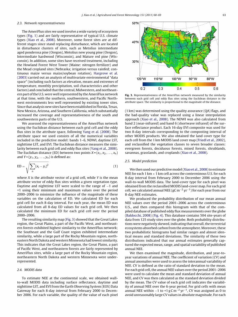
hold-out block is then used to test the performance of the model(RuleQuest, 2008). The 10-fold cross-validation also showed thatour model predicted NEE fairly well (Fig. 2; R2 = 0.67, p < 0.0001;RMSE = 1.45 gC m−2 day−1).

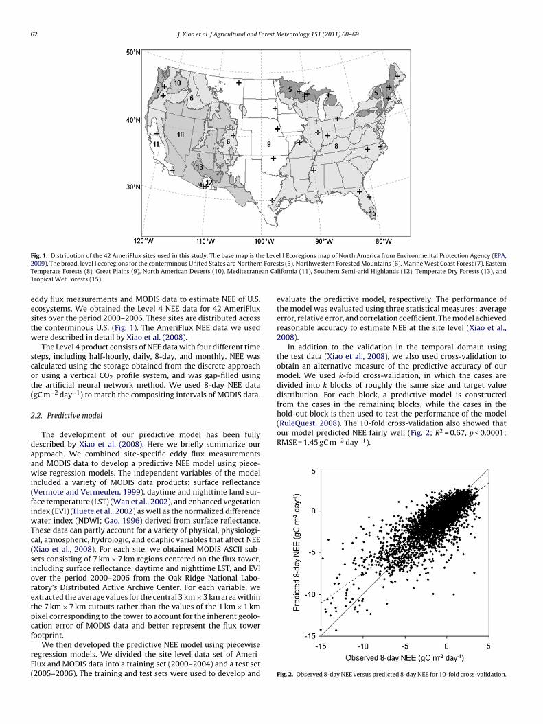
ig. 1. Distribution of the 42 AmeriFlux sites used in this study. The base map is th009). The broad, level I ecoregions for the conterminous United States are Northernemperate Forests (8), Great Plains (9), North American Deserts (10), Mediterraneropical Wet Forests (15).

ddy flux measurements and MODIS data to estimate NEE of U.S.cosystems. We obtained the Level 4 NEE data for 42 AmeriFluxites over the period 2000–2006. These sites are distributed acrosshe conterminous U.S. (Fig. 1). The AmeriFlux NEE data we usedere described in detail by Xiao et al. (2008).

The Level 4 product consists of NEE data with four different timeteps, including half-hourly, daily, 8-day, and monthly. NEE wasalculated using the storage obtained from the discrete approachr using a vertical CO2 profile system, and was gap-filled usinghe artificial neural network method. We used 8-day NEE datagC m−2 day−1) to match the compositing intervals of MODIS data.

.2. Predictive model

The development of our predictive model has been fullyescribed by Xiao et al. (2008). Here we briefly summarize ourpproach. We combined site-specific eddy flux measurementsnd MODIS data to develop a predictive NEE model using piece-ise regression models. The independent variables of the model

ncluded a variety of MODIS data products: surface reflectanceVermote and Vermeulen, 1999), daytime and nighttime land sur-ace temperature (LST) (Wan et al., 2002), and enhanced vegetationndex (EVI) (Huete et al., 2002) as well as the normalized difference

ater index (NDWI; Gao, 1996) derived from surface reflectance.hese data can partly account for a variety of physical, physiologi-al, atmospheric, hydrologic, and edaphic variables that affect NEEXiao et al., 2008). For each site, we obtained MODIS ASCII sub-ets consisting of 7 km × 7 km regions centered on the flux tower,ncluding surface reflectance, daytime and nighttime LST, and EVIver the period 2000–2006 from the Oak Ridge National Labo-atory’s Distributed Active Archive Center. For each variable, wextracted the average values for the central 3 km × 3 km area withinhe 7 km × 7 km cutouts rather than the values of the 1 km × 1 kmixel corresponding to the tower to account for the inherent geolo-ation error of MODIS data and better represent the flux tower

ootprint.

We then developed the predictive NEE model using piecewiseegression models. We divided the site-level data set of Ameri-lux and MODIS data into a training set (2000–2004) and a test set2005–2006). The training and test sets were used to develop and

l I Ecoregions map of North America from Environmental Protection Agency (EPA,ts (5), Northwestern Forested Mountains (6), Marine West Coast Forest (7), Easternlifornia (11), Southern Semi-arid Highlands (12), Temperate Dry Forests (13), and

evaluate the predictive model, respectively. The performance ofthe model was evaluated using three statistical measures: averageerror, relative error, and correlation coefficient. The model achievedreasonable accuracy to estimate NEE at the site level (Xiao et al.,2008).

In addition to the validation in the temporal domain usingthe test data (Xiao et al., 2008), we also used cross-validation toobtain an alternative measure of the predictive accuracy of ourmodel. We used k-fold cross-validation, in which the cases aredivided into k blocks of roughly the same size and target valuedistribution. For each block, a predictive model is constructedfrom the cases in the remaining blocks, while the cases in the

Fig. 2. Observed 8-day NEE versus predicted 8-day NEE for 10-fold cross-validation.

orest Meteorology 151 (2011) 60–69 63

2

ttfiaIcttt(stfeawSNis

uflainlTa

E

waD+2vgcc2

retseToAnr

2

tnGb

J. Xiao et al. / Agricultural and F

.3. Network representativeness

The AmeriFlux sites we used involve a wide variety of ecosystemypes (Fig. 1) and are fairly representative of typical U.S. climateypes (Xiao et al., 2008). Moreover, some forest sites are at dif-erent stages since stand replacing disturbance, which are locatedn disturbance clusters of sites, such as Metolius intermediateged ponderosa pine (Oregon), Metolius new young pine (Oregon),ntermediate hardwood (Wisconsin), and Mature red pine (Wis-onsin). In addition, some sites have received treatment, includinghe Howland Forest West Tower (Maine: nitrogen fertilizer) andhe Mead cropland sites (Nebraska; irrigation versus rainfed; con-inuous maize versus maize/soybean rotation). Hargrove et al.2003) carried out an analysis of multivariate environmental “datapace” (including such factors as elevation, means and extremes ofemperature, monthly precipitation, soil characteristics and otheractors) and concluded that the central, Midwestern, and northeast-rn part of the U.S. were well represented by the AmeriFlux networkt that time, with the southern, southwestern, and Pacific North-est environments less well represented by existing tower sites.

ince that analysis new sites have been established in Florida, Texas,ew Mexico, Arizona, and Southern California, which substantially

ncreased the coverage and representativeness of the south andouthwestern parts of the U.S.

We assessed the representativeness of the AmeriFlux networksing the Euclidean distance between each grid cell and the eddyux sites in the attribute space, following Yang et al. (2008). Thettribute space we used consists of all the numerical variablesncluded in the predictive model: bands 1–6, NDWI, daytime LST,ighttime LST, and EVI. The Euclidean distance measures the simi-

arity between each grid cell and eddy flux sites (Yang et al., 2008).he Euclidian distance (ED) between two points X = (x1, x2, . . ., xn)nd Y = (y1, y2, . . ., yn) is defined as:

D =√∑

n

(xi − yi)2 (1)

here X is the attribute vector of a grid cell, while Y is the meanttribute vector of eddy flux sites within a given vegetation type.aytime and nighttime LST were scaled to the range of −1 and1 using their minimum and maximum values over the period000–2006 to minimize the influence of the magnitude of theseariables on the calculation of ED. We calculated ED for eachrid cell for each 8-day interval. For each year, the mean ED wasalculated from all 8-day ED values for each grid cell. We thenalculated the minimum ED for each grid cell over the period000–2006.

The resulting similarity map (Fig. 3) showed that the Great Lakesegion, the Great Plains, a part of the Pacific West, and northeast-rn forests exhibited highest similarity to the AmeriFlux network;he Southeast and the Gulf Coast region exhibited intermediateimilarity, while a large part of the Rocky Mountain region, north-astern North Dakota and western Minnesota had lowest similarity.his indicates that the Great Lakes region, the Great Plains, a partf Pacific West, and northeastern forests are fairly represented bymeriFlux sites, while a large part of the Rocky Mountain region,ortheastern North Dakota and western Minnesota were under-epresented.

.4. MODIS data

To estimate NEE at the continental scale, we obtained wall-o-wall MODIS data including surface reflectance, daytime andighttime LST, and EVI from the Earth Observing System (EOS) Dataateway for each 8-day interval from February 2000 to Decem-er 2006. For each variable, the quality of the value of each pixel

Fig. 3. Representativeness of the AmeriFlux network measured by the similaritybetween each grid cell and eddy flux sites using the Euclidean distance in theattribute space. The similarity is proportional to the magnitude of the distance.

(1 km) was determined using the quality assurance (QA) flags, andthe bad-quality value was replaced using a linear interpolationapproach (Xiao et al., 2008). The NDWI was also calculated fromband 2 (near-infrared) and band 6 (shortwave infrared) of the sur-face reflectance product. Each 16-day EVI composite was used fortwo 8-day intervals corresponding to the composting interval ofother MODIS products. We also obtained the land cover type foreach cell from the 1 km MODIS land cover map (Friedl et al., 2002),and reclassified the vegetation classes to seven broader classes:evergreen forests, deciduous forests, mixed forests, shrublands,savannas, grasslands, and croplands (Xiao et al., 2008).

2.5. Model prediction

We then used our predictive model (Xiao et al., 2008) to estimateNEE for each 1 km × 1 km cell across the conterminous U.S. for each8-day interval from February 2000 to December 2006 using thewall-to-wall MODIS data. The land-cover type for each pixel wasobtained from the reclassified MODIS land-cover map. For each gridcell, we calculated annual NEE (gC m−2 yr−1) for each year from our8-day NEE estimates.

We produced the probability distribution of our mean annualNEE values over the period 2001–2006 across the conterminousU.S., and then compared this histogram with that of the com-piled database of published eddy flux measurements over the globe(Baldocchi, 2008) (Fig. 4). This database contains 504 site-years ofdata from 125 study sites over the globe. Both probability distribu-tions were negatively skewed, indicating that overall, the terrestrialecosystems absorbed carbon from the atmosphere. Moreover, thesetwo probabilistic histograms had similar ranges and almost iden-tical means and standard deviations. The similarity of these twodistributions indicated that our annual estimates generally cap-tured the expected mean, range, and spatial variability of publishedannual NEE.

We then examined the magnitude, distribution, and year-to-year variations of annual NEE. The coefficient of variation (CV) andannual anomalies were used to assess the interannual variability ofNEE. CV is defined as the ratio of standard deviation to the mean.For each grid cell, the annual NEE values over the period 2001–2006were used to calculate the mean and standard deviation of annual

NEE, and CV was then calculated as the standard deviation dividedby the mean. The CV value of each grid cell indicates the variabil-ity of annual NEE over the 6-year period. For grid cells with meanannual NEE within −1 to +1 g C m−2 yr−1, CV was assigned as 0 toavoid unreasonably large CV values in absolute magnitude. For each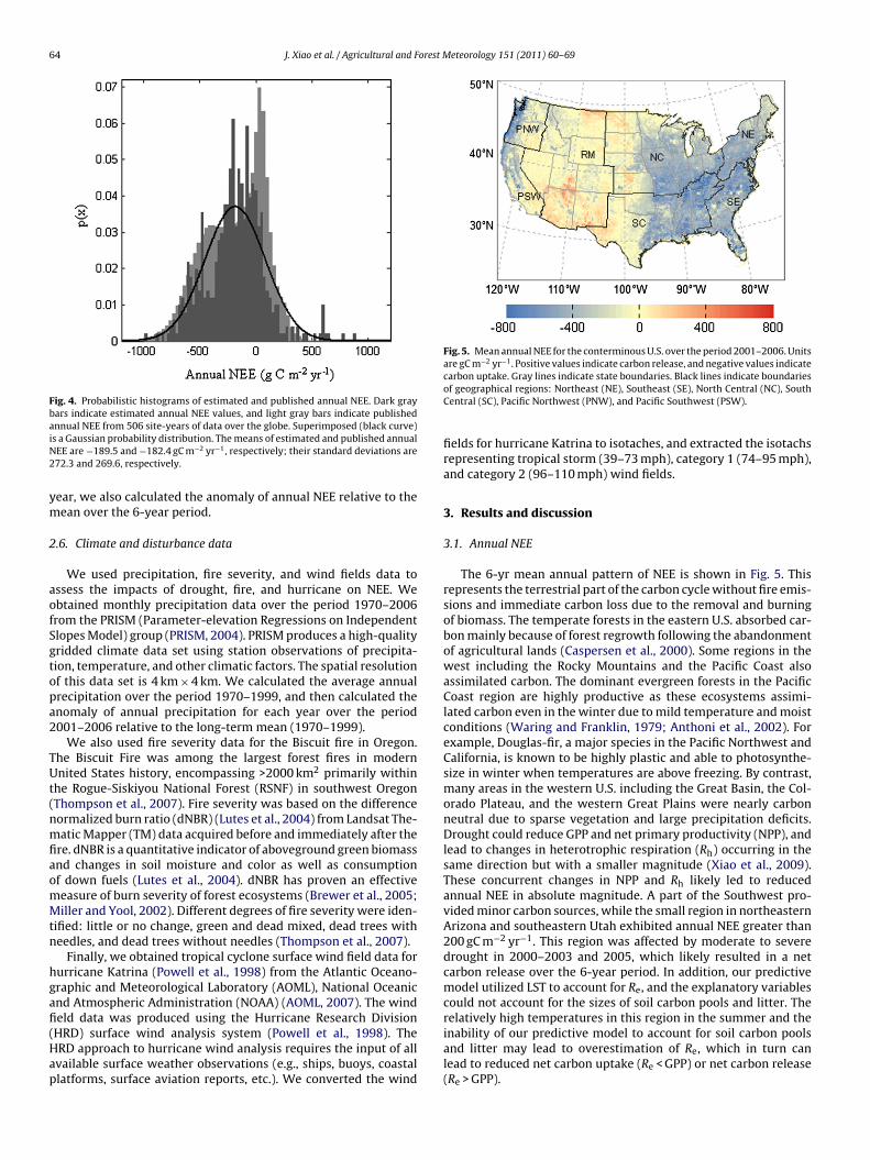

64 J. Xiao et al. / Agricultural and Forest Meteorology 151 (2011) 60–69

Fig. 4. Probabilistic histograms of estimated and published annual NEE. Dark graybars indicate estimated annual NEE values, and light gray bars indicate publishedaiN2

ym

2

aofSgtopa2

TUt(nmfiaomMtn

hgafi(Hap

Fig. 5. Mean annual NEE for the conterminous U.S. over the period 2001–2006. Unitsare gC m−2 yr−1. Positive values indicate carbon release, and negative values indicate

nnual NEE from 506 site-years of data over the globe. Superimposed (black curve)s a Gaussian probability distribution. The means of estimated and published annualEE are −189.5 and −182.4 gC m−2 yr−1, respectively; their standard deviations are72.3 and 269.6, respectively.

ear, we also calculated the anomaly of annual NEE relative to theean over the 6-year period.

.6. Climate and disturbance data

We used precipitation, fire severity, and wind fields data tossess the impacts of drought, fire, and hurricane on NEE. Webtained monthly precipitation data over the period 1970–2006rom the PRISM (Parameter-elevation Regressions on Independentlopes Model) group (PRISM, 2004). PRISM produces a high-qualityridded climate data set using station observations of precipita-ion, temperature, and other climatic factors. The spatial resolutionf this data set is 4 km × 4 km. We calculated the average annualrecipitation over the period 1970–1999, and then calculated thenomaly of annual precipitation for each year over the period001–2006 relative to the long-term mean (1970–1999).

We also used fire severity data for the Biscuit fire in Oregon.he Biscuit Fire was among the largest forest fires in modernnited States history, encompassing >2000 km2 primarily within

he Rogue-Siskiyou National Forest (RSNF) in southwest OregonThompson et al., 2007). Fire severity was based on the differenceormalized burn ratio (dNBR) (Lutes et al., 2004) from Landsat The-atic Mapper (TM) data acquired before and immediately after the

re. dNBR is a quantitative indicator of aboveground green biomassnd changes in soil moisture and color as well as consumptionf down fuels (Lutes et al., 2004). dNBR has proven an effectiveeasure of burn severity of forest ecosystems (Brewer et al., 2005;iller and Yool, 2002). Different degrees of fire severity were iden-

ified: little or no change, green and dead mixed, dead trees witheedles, and dead trees without needles (Thompson et al., 2007).

Finally, we obtained tropical cyclone surface wind field data forurricane Katrina (Powell et al., 1998) from the Atlantic Oceano-raphic and Meteorological Laboratory (AOML), National Oceanicnd Atmospheric Administration (NOAA) (AOML, 2007). The wind

eld data was produced using the Hurricane Research DivisionHRD) surface wind analysis system (Powell et al., 1998). TheRD approach to hurricane wind analysis requires the input of allvailable surface weather observations (e.g., ships, buoys, coastallatforms, surface aviation reports, etc.). We converted the wind

carbon uptake. Gray lines indicate state boundaries. Black lines indicate boundariesof geographical regions: Northeast (NE), Southeast (SE), North Central (NC), SouthCentral (SC), Pacific Northwest (PNW), and Pacific Southwest (PSW).

fields for hurricane Katrina to isotaches, and extracted the isotachsrepresenting tropical storm (39–73 mph), category 1 (74–95 mph),and category 2 (96–110 mph) wind fields.

3. Results and discussion

3.1. Annual NEE

The 6-yr mean annual pattern of NEE is shown in Fig. 5. Thisrepresents the terrestrial part of the carbon cycle without fire emis-sions and immediate carbon loss due to the removal and burningof biomass. The temperate forests in the eastern U.S. absorbed car-bon mainly because of forest regrowth following the abandonmentof agricultural lands (Caspersen et al., 2000). Some regions in thewest including the Rocky Mountains and the Pacific Coast alsoassimilated carbon. The dominant evergreen forests in the PacificCoast region are highly productive as these ecosystems assimi-lated carbon even in the winter due to mild temperature and moistconditions (Waring and Franklin, 1979; Anthoni et al., 2002). Forexample, Douglas-fir, a major species in the Pacific Northwest andCalifornia, is known to be highly plastic and able to photosynthe-size in winter when temperatures are above freezing. By contrast,many areas in the western U.S. including the Great Basin, the Col-orado Plateau, and the western Great Plains were nearly carbonneutral due to sparse vegetation and large precipitation deficits.Drought could reduce GPP and net primary productivity (NPP), andlead to changes in heterotrophic respiration (Rh) occurring in thesame direction but with a smaller magnitude (Xiao et al., 2009).These concurrent changes in NPP and Rh likely led to reducedannual NEE in absolute magnitude. A part of the Southwest pro-vided minor carbon sources, while the small region in northeasternArizona and southeastern Utah exhibited annual NEE greater than200 gC m−2 yr−1. This region was affected by moderate to severedrought in 2000–2003 and 2005, which likely resulted in a netcarbon release over the 6-year period. In addition, our predictivemodel utilized LST to account for Re, and the explanatory variablescould not account for the sizes of soil carbon pools and litter. Therelatively high temperatures in this region in the summer and the

inability of our predictive model to account for soil carbon poolsand litter may lead to overestimation of Re, which in turn canlead to reduced net carbon uptake (Re < GPP) or net carbon release(Re > GPP).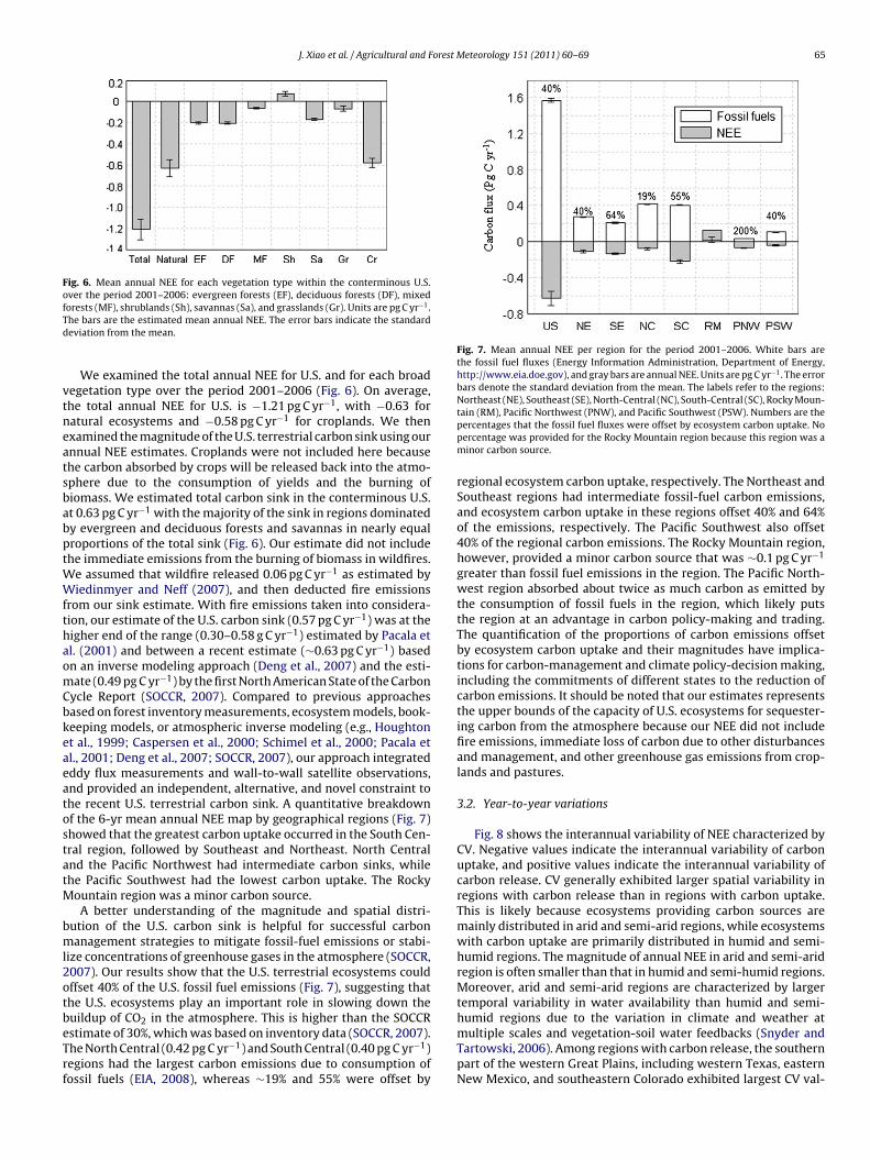

J. Xiao et al. / Agricultural and Forest Meteorology 151 (2011) 60–69 65

Fig. 6. Mean annual NEE for each vegetation type within the conterminous U.S.over the period 2001–2006: evergreen forests (EF), deciduous forests (DF), mixedfTd

vtneatsbabptWWfthaomCbkeaeatostatM

bml2otbeTrf

Fig. 7. Mean annual NEE per region for the period 2001–2006. White bars arethe fossil fuel fluxes (Energy Information Administration, Department of Energy,http://www.eia.doe.gov), and gray bars are annual NEE. Units are pg C yr−1. The errorbars denote the standard deviation from the mean. The labels refer to the regions:Northeast (NE), Southeast (SE), North-Central (NC), South-Central (SC), Rocky Moun-

humid regions due to the variation in climate and weather at

orests (MF), shrublands (Sh), savannas (Sa), and grasslands (Gr). Units are pg C yr−1.he bars are the estimated mean annual NEE. The error bars indicate the standardeviation from the mean.

We examined the total annual NEE for U.S. and for each broadegetation type over the period 2001–2006 (Fig. 6). On average,he total annual NEE for U.S. is −1.21 pg C yr−1, with −0.63 foratural ecosystems and −0.58 pg C yr−1 for croplands. We thenxamined the magnitude of the U.S. terrestrial carbon sink using ournnual NEE estimates. Croplands were not included here becausehe carbon absorbed by crops will be released back into the atmo-phere due to the consumption of yields and the burning ofiomass. We estimated total carbon sink in the conterminous U.S.t 0.63 pg C yr−1 with the majority of the sink in regions dominatedy evergreen and deciduous forests and savannas in nearly equalroportions of the total sink (Fig. 6). Our estimate did not includehe immediate emissions from the burning of biomass in wildfires.

e assumed that wildfire released 0.06 pg C yr−1 as estimated byiedinmyer and Neff (2007), and then deducted fire emissions

rom our sink estimate. With fire emissions taken into considera-ion, our estimate of the U.S. carbon sink (0.57 pg C yr−1) was at theigher end of the range (0.30–0.58 g C yr−1) estimated by Pacala etl. (2001) and between a recent estimate (∼0.63 pg C yr−1) basedn an inverse modeling approach (Deng et al., 2007) and the esti-ate (0.49 pg C yr−1) by the first North American State of the Carbon

ycle Report (SOCCR, 2007). Compared to previous approachesased on forest inventory measurements, ecosystem models, book-eeping models, or atmospheric inverse modeling (e.g., Houghtont al., 1999; Caspersen et al., 2000; Schimel et al., 2000; Pacala etl., 2001; Deng et al., 2007; SOCCR, 2007), our approach integratedddy flux measurements and wall-to-wall satellite observations,nd provided an independent, alternative, and novel constraint tohe recent U.S. terrestrial carbon sink. A quantitative breakdownf the 6-yr mean annual NEE map by geographical regions (Fig. 7)howed that the greatest carbon uptake occurred in the South Cen-ral region, followed by Southeast and Northeast. North Centralnd the Pacific Northwest had intermediate carbon sinks, whilehe Pacific Southwest had the lowest carbon uptake. The Rocky

ountain region was a minor carbon source.A better understanding of the magnitude and spatial distri-

ution of the U.S. carbon sink is helpful for successful carbonanagement strategies to mitigate fossil-fuel emissions or stabi-

ize concentrations of greenhouse gases in the atmosphere (SOCCR,007). Our results show that the U.S. terrestrial ecosystems couldffset 40% of the U.S. fossil fuel emissions (Fig. 7), suggesting thathe U.S. ecosystems play an important role in slowing down theuildup of CO2 in the atmosphere. This is higher than the SOCCR

stimate of 30%, which was based on inventory data (SOCCR, 2007).he North Central (0.42 pg C yr−1) and South Central (0.40 pg C yr−1)egions had the largest carbon emissions due to consumption ofossil fuels (EIA, 2008), whereas ∼19% and 55% were offset by

tain (RM), Pacific Northwest (PNW), and Pacific Southwest (PSW). Numbers are thepercentages that the fossil fuel fluxes were offset by ecosystem carbon uptake. Nopercentage was provided for the Rocky Mountain region because this region was aminor carbon source.

regional ecosystem carbon uptake, respectively. The Northeast andSoutheast regions had intermediate fossil-fuel carbon emissions,and ecosystem carbon uptake in these regions offset 40% and 64%of the emissions, respectively. The Pacific Southwest also offset40% of the regional carbon emissions. The Rocky Mountain region,however, provided a minor carbon source that was ∼0.1 pg C yr−1

greater than fossil fuel emissions in the region. The Pacific North-west region absorbed about twice as much carbon as emitted bythe consumption of fossil fuels in the region, which likely putsthe region at an advantage in carbon policy-making and trading.The quantification of the proportions of carbon emissions offsetby ecosystem carbon uptake and their magnitudes have implica-tions for carbon-management and climate policy-decision making,including the commitments of different states to the reduction ofcarbon emissions. It should be noted that our estimates representsthe upper bounds of the capacity of U.S. ecosystems for sequester-ing carbon from the atmosphere because our NEE did not includefire emissions, immediate loss of carbon due to other disturbancesand management, and other greenhouse gas emissions from crop-lands and pastures.

3.2. Year-to-year variations

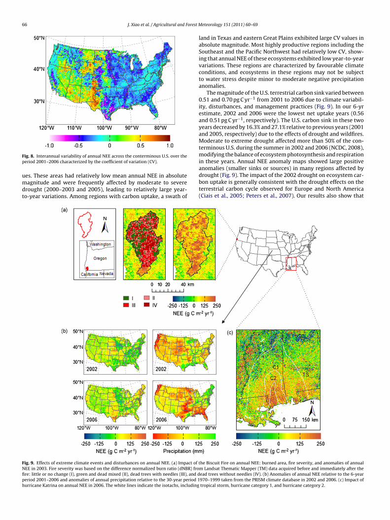
Fig. 8 shows the interannual variability of NEE characterized byCV. Negative values indicate the interannual variability of carbonuptake, and positive values indicate the interannual variability ofcarbon release. CV generally exhibited larger spatial variability inregions with carbon release than in regions with carbon uptake.This is likely because ecosystems providing carbon sources aremainly distributed in arid and semi-arid regions, while ecosystemswith carbon uptake are primarily distributed in humid and semi-humid regions. The magnitude of annual NEE in arid and semi-aridregion is often smaller than that in humid and semi-humid regions.Moreover, arid and semi-arid regions are characterized by largertemporal variability in water availability than humid and semi-

multiple scales and vegetation-soil water feedbacks (Snyder andTartowski, 2006). Among regions with carbon release, the southernpart of the western Great Plains, including western Texas, easternNew Mexico, and southeastern Colorado exhibited largest CV val-

66 J. Xiao et al. / Agricultural and Forest M

Fp

umdt

FNfiph

ig. 8. Interannual variability of annual NEE across the conterminous U.S. over theeriod 2001–2006 characterized by the coefficient of variation (CV).

es. These areas had relatively low mean annual NEE in absoluteagnitude and were frequently affected by moderate to severe

rought (2000–2003 and 2005), leading to relatively large year-o-year variations. Among regions with carbon uptake, a swath of

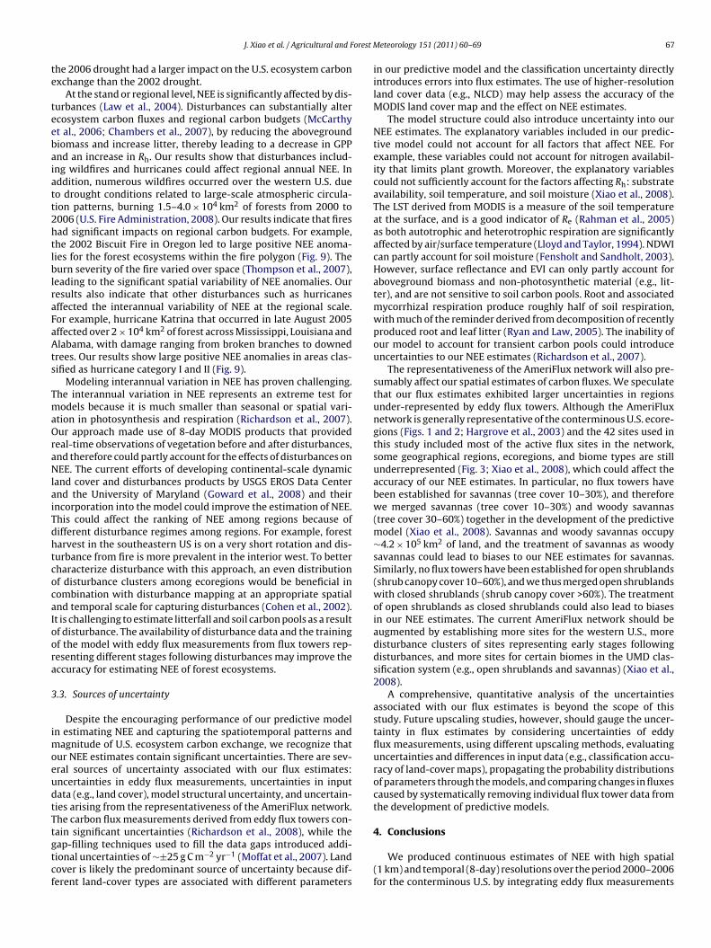
ig. 9. Effects of extreme climate events and disturbances on annual NEE. (a) Impact of tEE in 2003. Fire severity was based on the difference normalized burn ratio (dNBR) frore: little or no change (I), green and dead mixed (II), dead trees with needles (III), and deriod 2001–2006 and anomalies of annual precipitation relative to the 30-year period 1urricane Katrina on annual NEE in 2006. The white lines indicate the isotachs, including

eteorology 151 (2011) 60–69

land in Texas and eastern Great Plains exhibited large CV values inabsolute magnitude. Most highly productive regions including theSoutheast and the Pacific Northwest had relatively low CV, show-ing that annual NEE of these ecosystems exhibited low year-to-yearvariations. These regions are characterized by favourable climateconditions, and ecosystems in these regions may not be subjectto water stress despite minor to moderate negative precipitationanomalies.

The magnitude of the U.S. terrestrial carbon sink varied between0.51 and 0.70 pg C yr−1 from 2001 to 2006 due to climate variabil-ity, disturbances, and management practices (Fig. 9). In our 6-yrestimate, 2002 and 2006 were the lowest net uptake years (0.56and 0.51 pg C yr−1, respectively). The U.S. carbon sink in these twoyears decreased by 16.3% and 27.1% relative to previous years (2001and 2005, respectively) due to the effects of drought and wildfires.Moderate to extreme drought affected more than 50% of the con-terminous U.S. during the summer in 2002 and 2006 (NCDC, 2008),modifying the balance of ecosystem photosynthesis and respirationin these years. Annual NEE anomaly maps showed large positive

anomalies (smaller sinks or sources) in many regions affected bydrought (Fig. 9). The impact of the 2002 drought on ecosystem car-bon uptake is generally consistent with the drought effects on theterrestrial carbon cycle observed for Europe and North America(Ciais et al., 2005; Peters et al., 2007). Our results also show that

he Biscuit Fire on annual NEE: burned area, fire severity, and anomalies of annualm Landsat Thematic Mapper (TM) data acquired before and immediately after theead trees without needles (IV). (b) Anomalies of annual NEE relative to the 6-year970–1999 taken from the PRISM climate database in 2002 and 2006. (c) Impact oftropical storm, hurricane category 1, and hurricane category 2.

orest M

te

teebaiatt2htlblraFaAts

TmaOraNlaiTdhtcocaIoora

3

imoeudtTtgtcf

J. Xiao et al. / Agricultural and F

he 2006 drought had a larger impact on the U.S. ecosystem carbonxchange than the 2002 drought.

At the stand or regional level, NEE is significantly affected by dis-urbances (Law et al., 2004). Disturbances can substantially altercosystem carbon fluxes and regional carbon budgets (McCarthyt al., 2006; Chambers et al., 2007), by reducing the abovegroundiomass and increase litter, thereby leading to a decrease in GPPnd an increase in Rh. Our results show that disturbances includ-ng wildfires and hurricanes could affect regional annual NEE. Inddition, numerous wildfires occurred over the western U.S. dueo drought conditions related to large-scale atmospheric circula-ion patterns, burning 1.5–4.0 × 104 km2 of forests from 2000 to006 (U.S. Fire Administration, 2008). Our results indicate that firesad significant impacts on regional carbon budgets. For example,he 2002 Biscuit Fire in Oregon led to large positive NEE anoma-ies for the forest ecosystems within the fire polygon (Fig. 9). Theurn severity of the fire varied over space (Thompson et al., 2007),

eading to the significant spatial variability of NEE anomalies. Ouresults also indicate that other disturbances such as hurricanesffected the interannual variability of NEE at the regional scale.or example, hurricane Katrina that occurred in late August 2005ffected over 2 × 104 km2 of forest across Mississippi, Louisiana andlabama, with damage ranging from broken branches to downed

rees. Our results show large positive NEE anomalies in areas clas-ified as hurricane category I and II (Fig. 9).

Modeling interannual variation in NEE has proven challenging.he interannual variation in NEE represents an extreme test forodels because it is much smaller than seasonal or spatial vari-

tion in photosynthesis and respiration (Richardson et al., 2007).ur approach made use of 8-day MODIS products that provided

eal-time observations of vegetation before and after disturbances,nd therefore could partly account for the effects of disturbances onEE. The current efforts of developing continental-scale dynamic

and cover and disturbances products by USGS EROS Data Centernd the University of Maryland (Goward et al., 2008) and theirncorporation into the model could improve the estimation of NEE.his could affect the ranking of NEE among regions because ofifferent disturbance regimes among regions. For example, forestarvest in the southeastern US is on a very short rotation and dis-urbance from fire is more prevalent in the interior west. To betterharacterize disturbance with this approach, an even distributionf disturbance clusters among ecoregions would be beneficial inombination with disturbance mapping at an appropriate spatialnd temporal scale for capturing disturbances (Cohen et al., 2002).t is challenging to estimate litterfall and soil carbon pools as a resultf disturbance. The availability of disturbance data and the trainingf the model with eddy flux measurements from flux towers rep-esenting different stages following disturbances may improve theccuracy for estimating NEE of forest ecosystems.

.3. Sources of uncertainty

Despite the encouraging performance of our predictive modeln estimating NEE and capturing the spatiotemporal patterns and

agnitude of U.S. ecosystem carbon exchange, we recognize thatur NEE estimates contain significant uncertainties. There are sev-ral sources of uncertainty associated with our flux estimates:ncertainties in eddy flux measurements, uncertainties in inputata (e.g., land cover), model structural uncertainty, and uncertain-ies arising from the representativeness of the AmeriFlux network.he carbon flux measurements derived from eddy flux towers con-

ain significant uncertainties (Richardson et al., 2008), while theap-filling techniques used to fill the data gaps introduced addi-ional uncertainties of ∼±25 g C m−2 yr−1 (Moffat et al., 2007). Landover is likely the predominant source of uncertainty because dif-erent land-cover types are associated with different parameters

eteorology 151 (2011) 60–69 67

in our predictive model and the classification uncertainty directlyintroduces errors into flux estimates. The use of higher-resolutionland cover data (e.g., NLCD) may help assess the accuracy of theMODIS land cover map and the effect on NEE estimates.

The model structure could also introduce uncertainty into ourNEE estimates. The explanatory variables included in our predic-tive model could not account for all factors that affect NEE. Forexample, these variables could not account for nitrogen availabil-ity that limits plant growth. Moreover, the explanatory variablescould not sufficiently account for the factors affecting Rh: substrateavailability, soil temperature, and soil moisture (Xiao et al., 2008).The LST derived from MODIS is a measure of the soil temperatureat the surface, and is a good indicator of Re (Rahman et al., 2005)as both autotrophic and heterotrophic respiration are significantlyaffected by air/surface temperature (Lloyd and Taylor, 1994). NDWIcan partly account for soil moisture (Fensholt and Sandholt, 2003).However, surface reflectance and EVI can only partly account foraboveground biomass and non-photosynthetic material (e.g., lit-ter), and are not sensitive to soil carbon pools. Root and associatedmycorrhizal respiration produce roughly half of soil respiration,with much of the reminder derived from decomposition of recentlyproduced root and leaf litter (Ryan and Law, 2005). The inability ofour model to account for transient carbon pools could introduceuncertainties to our NEE estimates (Richardson et al., 2007).

The representativeness of the AmeriFlux network will also pre-sumably affect our spatial estimates of carbon fluxes. We speculatethat our flux estimates exhibited larger uncertainties in regionsunder-represented by eddy flux towers. Although the AmeriFluxnetwork is generally representative of the conterminous U.S. ecore-gions (Figs. 1 and 2; Hargrove et al., 2003) and the 42 sites used inthis study included most of the active flux sites in the network,some geographical regions, ecoregions, and biome types are stillunderrepresented (Fig. 3; Xiao et al., 2008), which could affect theaccuracy of our NEE estimates. In particular, no flux towers havebeen established for savannas (tree cover 10–30%), and thereforewe merged savannas (tree cover 10–30%) and woody savannas(tree cover 30–60%) together in the development of the predictivemodel (Xiao et al., 2008). Savannas and woody savannas occupy∼4.2 × 105 km2 of land, and the treatment of savannas as woodysavannas could lead to biases to our NEE estimates for savannas.Similarly, no flux towers have been established for open shrublands(shrub canopy cover 10–60%), and we thus merged open shrublandswith closed shrublands (shrub canopy cover >60%). The treatmentof open shrublands as closed shrublands could also lead to biasesin our NEE estimates. The current AmeriFlux network should beaugmented by establishing more sites for the western U.S., moredisturbance clusters of sites representing early stages followingdisturbances, and more sites for certain biomes in the UMD clas-sification system (e.g., open shrublands and savannas) (Xiao et al.,2008).

A comprehensive, quantitative analysis of the uncertaintiesassociated with our flux estimates is beyond the scope of thisstudy. Future upscaling studies, however, should gauge the uncer-tainty in flux estimates by considering uncertainties of eddyflux measurements, using different upscaling methods, evaluatinguncertainties and differences in input data (e.g., classification accu-racy of land-cover maps), propagating the probability distributionsof parameters through the models, and comparing changes in fluxescaused by systematically removing individual flux tower data fromthe development of predictive models.

4. Conclusions

We produced continuous estimates of NEE with high spatial(1 km) and temporal (8-day) resolutions over the period 2000–2006for the conterminous U.S. by integrating eddy flux measurements

6 orest M

awEdtpaa

vocrniatvttrpn

A

FpuADTEddpCevr

rBDJKdMA

R

A

A

A

B

B

8 J. Xiao et al. / Agricultural and F

nd wall-to-wall MODIS data. Our continuous NEE estimates alongith our previous GPP estimates (Xiao et al., 2010), referred to as

C-MOD, were both derived from eddy covariance (EC) and MODISata. The EC-MOD dataset has high temporal and spatial resolu-ions, and are highly constrained by eddy covariance data. EC-MODrovides alternative, independent gridded flux estimates for U.S.,nd is useful for evaluating simulations of ecosystem models andtmospheric inversions.

We examined the spatial patterns, magnitude, and interannualariability of U.S. ecosystem carbon exchange using our continu-us NEE estimates. We estimated the terrestrial carbon sink in theonterminous U.S. at 0.63 pg C yr−1 with the majority of the sink inegions dominated by evergreen and deciduous forests and savan-as. Our results show that U.S. ecosystems play an important role

n slowing down the buildup of CO2 in the atmosphere. Our resultslso show that recent U.S. annual NEE exhibited significant year-o-year variations. The dominant sources of the recent interannualariation included extreme climate events (e.g., drought) and dis-urbances (e.g., wildfires, hurricanes). Our results also highlighthe need to improve our understanding of the impacts of stand-eplacing disturbances on the forest carbon budget. Our studyrovides an alternative, independent, and novel constraint to theet ecosystem carbon exchange of U.S. terrestrial ecosystems.

cknowledgements

This study was supported by grants from the National Scienceoundation (NSF) and Department of Energy (DOE). We thank therincipal investigators and contributors of the MODIS data prod-cts, the Oak Ridge National Laboratory (ORNL) Distributed Activerchive Center (DACCC), and the Earth Observing System (EOS)ata Gateway for making these MODIS data products available.he Level I Ecoregions map of North America was obtained fromnvironmental Protection Agency (EPA), the Biscuit fire severityata from J. Thompson, Harvard University, and the PRISM climateatabase from the PRISM Group, Oregon State University. Com-uting support was provided by the Rosen Center for Advancedomputing, Purdue University. We also thank anonymous review-rs and Dr. Anne Verhoef for their valuable comments on earlierersions of the manuscript. [The EC-MOD dataset is available uponequest.]

Contributors: J.X. and Q.Z. designed the study; J.X. conducted theesearch and analyzed the results; J.X. and Q.Z. wrote the paper;.E.L., D.D.B., J.C., A.D.R., K.J.D., D.Y.H., S.W., R.O., A.N., M.L.F., S.B.V.,.R.C., G.S., S.M., S.C.W., P.V.B., S.P.B., P.S.C., B.G.D., M.F., D.R.F., L.G.,

.L.H., G.G.K., M.L., S.M., T.A.M., R.M., T.P.M., R.K.M., J.W.M., W.C.O.,.T.P.U., H.P.S., R.L.S., G.S., A.E.S., and M.S.T. contributed eddy fluxata; B.E.L., D.D.B., J.C., A.D.R., J.M.M., K.J.D., D.Y.H., S.W., R.O., A.N.,.L.F., S.B.V., and D.R.C. provided comments on the manuscript.

uthors from P.V.B. to M.S.T. are listed alphabetically.

eferences

miro, B.D., Barr, A.G., Barr, J.G., Black, T.A., Bracho, R., Brown, M., Chen, J., Clark, K.L.,Davis, K.J., Desai, A.R., Dore, S., Engel, V., Fuentes, J.D., Goldstein, A.H., Goulden,M.L., Kolb, T.E., Lavigne, M.B., Law, B.E., Margolis, H.A., Martin, T., McCaughey,J.H., Misson, L., Montes-Helu, M., Noormets, A., Randerson, J.T., Starr, G., Xiao, J.,in press. Ecosystem carbon dioxide fluxes after disturbance in forests of NorthAmerica. J. Geophys. Res., doi:10.1029/2010JG001390.

nthoni, P.M., Unsworth, M.H., Law, B.E., Irvine, J., Baldocchi, D.D., Tuyl, S.V., Moore,D., 2002. Seasonal differences in carbon and water vapor exchange in young andold-growth ponderosa pine ecosystems. Agric. Forest Meteorol. 111, 203–222.

tlantic Oceanographic and Meteorological Laboratory (AOML), 2007.http://www.aoml.noaa.gov/hrd/Storm pages/katrina2005.

aldocchi, D.D., 2003. Asssessing the eddy covariance technique for evaluating car-bon dioxide exchange rates of ecosystems: past, present, and future. GlobalChange Biol. 9, 479–492.

aldocchi, D.D., Falge, E., Gu, L., Olson, R., Hollinger, D., Running, S., Anthoni, P.,Bernhofer, C., Davis, K., Evans, R., Fuentes, J., Goldstein, A., Katul, G., Law, B.,Lee, X., Malhi, Y., Meyers, T., Munger, W., Oechel, W., Paw, U.K.T., Pilegaard,

eteorology 151 (2011) 60–69

K., Schmid, H.P., Valentini, R., Verma, S., Vesala, T., Wilson, K., Wofsy, S., 2001.FLUXNET: a new tool to study the temporal and spatial variability of ecosystem-scale carbon dioxide, water vapor, and energy flux densities. Bull. Am. Meteorol.Soc. 82, 2415–2434.

Baldocchi, D., 2008. ‘Breathing’ of the terrestrial biosphere: lessons learned from aglobal network of carbon dioxide flux measurements systems. Aust. J. Bot. 56,1–26.

Brewer, C.K., Winne, J.C., Redmond, R.L., Opitz, D.W., Mangrich, M.V., 2005. Classify-ing and mapping wildfire severity: a comparison of methods. Photogram. Eng.Remote Sens. 71, 1311–1320.

Caspersen, J.P., Pacala, S.W., Jenkins, J.C., Hurtt, G.C., Moorcroft, P.R., Birdsey, R.A.,2000. Contributions of land-use history to carbon accumulation in U.S. forests.Science 290, 1148–1151.

Chambers, J.Q., Fisher, J.I., Zeng, H., Chapman, E.L., Baker, D.B., Hurtt, G.C., 2007. Hur-ricane Katrina’s carbon footprint on U.S. Gulf Coast Forest Sci. 318, 1107–11107.

Ciais, P.H., Reichstein, M., Viovy, N., Granier, A., Ogée, J., Allard, V., Aubinet, M.,Buchmann, N., Bernhofer, C., Carrara, A., Chevallier, F., Noblet, N.D., Friend, A.D.,Friedlingstein, P., Grünwald, T., Heinesch, B., Keronen, P., Knohl, A., Krinner, G.,Loustau, D., Manca, G., Matteucci, G., Miglietta, F., Ourcival, J.M., Papale, D., Pile-gaard, K., Rambal, S., Seufert, G., Soussana, J.F., Sanz, M.J., Schulze, E.D., Vesala,T., Valentini, R., 2005. Europe-wide reduction in primary productivity caused bythe heat and drought in 2003. Nature 437, 529–533.

Clark, D.A., Brown, S., Kicklighter, D.W., Chambers, J.Q., Thomlinson, J.R., Ni, J., 2001.Measuring net primary production in forests: concepts and field methods. Ecol.Appl. 11, 356–370.

Cohen, W.B., Spies, T.A., Alig, R.J., Oetter, D.R., Maiersperger, T.K., Fiorella, M., 2002.Characterizing 23 years (1972–1995) of stand replacement disturbance in west-ern Oregon forests with Landsat imagery. Ecosystems 5, 122–137.

Deng, F., Chen, J.M., Ishizawa, M., Yuen, C.-W., Mo, G., Higuchi, K., Chan, D., Maksyu-tov, S., 2007. Global monthly CO2 flux inversion with a focus over North America.Tellus 59B, 179–190.

Energy Information Administration, Department of Energy (DOE), 2008.http://www.eia.doe.gov.

Environmental Protection Agency (EPA), 2009, http://www.epa.gov/wed/pages/ecoregions.htm.

Fensholt, R., Sandholt, I., 2003. Derivation of a shortwave infrared water stress indexfrom MODIS near- and shortwave infrared data in a semiarid environment.Remote Sens. Environ. 87, 111–121.

Friedl, M.A., McIver, D.K., Hodges, J.C.F., Zhang, X.Y., Muchoney, D., Strahler, A.H.,Woodcock, C.E., Gopal, S., Schneider, A., Cooper, A., Baccini, A., Gao, F., Schaaf,C., 2002. Global land cover mapping from MODIS: algorithms and early results.Remote Sens. Environ. 83, 287–302.

Gao, B.C., 1996. NDWI—a normalized difference water index for remote sensing ofvegetation liquid water from space. Remote Sens. Environ. 58, 257–266.

Göckede, M., Foken, T., Aubinet, M., Aurela, M., Banaz, J., Bernhofer, C., Boonefond,J.M., Brunet, Y., Carrara, A., Clement, R., Dellwik, E., Elbers, J., Eugster, W., Fuhrer,J., Granier, A., Grünwald, T., Heinesch, B., Janssens, I.A., Knohl, A., Koeble, R., Lau-rila, T., Longdoz, B., Manca, G., Marek, M., Markkanen, T., Mateus, J., Matteucci,G., Mauder, M., Migliavacca, M., Minerbi, S., Moncrieff, J., Montagnani, L., Moors,E., Ourcival, J.-M., Papale, D., Pereira, J., Pilegaard, K., Pita, G., Rambal, S., Reb-mann, C., Rodrigues, A., Rotenberg, E., Sanz, M.J., Sedlak, P., Seufert, G., Siebicke,L., Soussana, J.F., Valentini, R., Vesala, T., Verbeeck, H., Yakir, D., 2008. Qualitycontrol of CarboEurope flux data. Part 1. Coupling footprint analyses with fluxdata quality assessment to evaluate sites in forest ecosystems. Biogeosciences5, 433–450.

Goodale, C.L., Apps, M.J., Birdsey, R.A., Field, C.B., Heath, L.S., Houghton, R.A., Jenkins,J.C., Kohlmaier, G.H., Kurz, W., Liu, S., Nabuurs, G.-J., Nilsson, S., Shvidenko, A.Z.,2002. Forest carbon sinks in the Northern Hemisphere. Ecol. Appl. 12, 891–899.

Goward, S.N., Masek, J.G., Cohen, W., Moisen, G., Collatz, G.J., Healey, S., Houghton,R.A., Huang, C., Kennedy, R., Law, B., Powell, S., Turner, D., Wulder, M.A.,2008. Forest disturbance and North American carbon flux. EOS Trans. AGU 89,doi:10.1029/2008EO110001.

Hargrove, W.W., Hoffman, F.M., Law, B.E., 2003. New analysis reveals representa-tiveness of the AmeriFlux network. EOS Trans. 84, 529–544.

Houghton, R.A., Hackler, J.L., Lawrence, K.T., 1999. The U.S. carbon budget: contribu-tions from land-use change. Science 285, 574–578.

Huete, A., Didan, K., Miura, T., Rodriguez, E.P., Gao, X., Ferreira, L.G., 2002. Overview ofthe radiometric and biophysical performance of the MODIS vegetation indices.Remote Sens. Environ. 83, 195–213.

Intergovernmental Panel on Climate Change, Climate Change 2007 – The PhysicalScience Basis, 2007. Contribution of Working Group I to the Fourth AssessmentReport of the IPCC. Cambridge University Press, New York.

Lal, R., Kimble, J.M., Follett, R.F., Stewart, B.A., 2001. Assessment Methods for SoilCarbon. Advances in Soil Science. Lewis Press, Boca Raton, FL, pp. 676.

Law, B.E., Turner, D., Campbell, J., Sun, O.J., Tuyl, S.V., Ritts, W.D., Cohen, W.B., 2004.Disturbances and climate effects on carbon stocks and fluxes across WesternOregon USA. Global Change Biol. 10, 1429–1444.

Lloyd, J., Taylor, J.A., 1994. On the temperature dependence of soil respiration. Funct.Ecol. 8, 315–323.

Lutes, D.C., Keane, J.F., Caratti, C.H., Key, C.H., Benson, N.C., Gangi, L.J., 2004. FIREMON:

Fire Effects Monitoring and Inventory System (US Department of AgricultureForest Service, Rocky Mountain Research Station, Ogden, UT), Vol. RMRS-GTR-164-CD, p. 400.

McCarthy, H.R., Oren, R., Kim, H.-S., Johnsen, K.H., Maier, C., Pritchard, S.G.,Davis, M.A., 2006. Interaction of ice storms and management practices oncurrent carbon sequestration in forests with potential mitigation under

orest M

M

M

P

P

P

P

PR

R

R

RR

S

S

S

S

J. Xiao et al. / Agricultural and F

future CO2 atmosphere. J. Geophys. Res. 111, doi:10.1029/2005JD006428,D15103.

iller, J.D., Yool, S.R., 2002. Mapping forest post-fire canopy consumption in severaloverstory types using multi-temporal Landsat TM and ETM data. Remote Sens.Environ. 82, 481–496.

offat, A.M., Papale, D., Reichstein, M., Hollinger, D.Y., Richardson, A.D., Barr,A.G., Beckstein, C., Braswell, B.H., Churkina, G., Desai, A.R., Falge, E., Gove, J.H.,Heimann, M., Hui, D., Jarvis, A.J., Kattge, J., Noormets, A., Stauch, V.J., 2007. Com-prehensive comparison of gap-filling techniques for eddy covariance net carbonfluxes. Agric. Forest Meteorol. 147, 209–232.

acala, S.W., Hurtt, G.C., Baker, D., Peylin, P., Houghton, R.A., Birdsey, R.A., Heath,L., Sundquist, E.T., Stallard, R.F., Ciais, P., Moorcroft, P., Caspersen, J.P., Shevli-akova, E., Moore, B., Kohlmaier, G., Holland, E., Gloor, M., Harmon, M.E., Fan,S.M., Sarmiento, J.L., Goodale, C.L., Schimel, D., Field, C.B., 2001. Consistent land-and atmosphere-based U.S. carbon sink estimates. Science 292, 2316–2320.

apale, D., Valentini, A., 2003. A new assessment of European forests carbonexchange by eddy fluxes and artificial neural network spatialization. GlobalChange Biol. 9, 525–535.

eters, W.P., Jacobson, A.R., Sweeney, C., Andrews, A.E., Conway, T.J., Masarie, K.,Miller, J.B., Bruhwiler, L.M.P., Pétron, G., Hirsch, A.I., Worthy, D.E.J., van der Werf,G.R., Randerson, J.T., Wennberg, P.O., Krol, M.C., Tans, P.P., 2007. An atmosphericperspective on North American carbon dioxide exchange: carbontracker. Proc.Natl. Acad. Sci. U.S.A. 104, 18925–18930.

owell, M.D., Houston, S.H., Amat, L.R., Morisseau-Leroy, N., 1998. The HRD real-timehurricane wind analysis system. J. Wind Eng. Indus. Aero. 77–78, 53–64.

RISM Group, 2004. Oregon State University, http://www.prismclimate.org.ahman, A.F., Sims, D.A., Cordova, V.D., El-Masri, B.Z., 2005. Potential of MODIS EVI

and surface temperature for directly estimating per-pixel ecosystem C fluxes.Geophys. Res. Lett. 32, doi:10.1029/2005GL024127, L19404.

ichardson, A.D., Hollinger, D.Y., Aber, J.D., Ollinger, S.V., Braswell, B.H., 2007. Envi-ronmental variation is directly responsible for short- but not long-term variationin forest-atmosphere carbon exchange. Global Change Biol. 13, 788–803.

ichardson, A.D., Mahecha, M.D., Falge, E., Kattge, J., Moffat, A.M., Papale, D., Reich-stein, M., Stauch, V.J., Braswell, B.H., Churkina, G., Kruijt, B., Hollinger, D.Y., 2008.Statistical properties of random CO flux measurement uncertainty inferred frommodel residuals. Agric. Forest Meteorol. 148, 38–50.

uleQuest, 2008. http://www.rulequest.com. Visited on 10/18/2007.yan, M.G., Law, B.E., 2005. Interpreting, measuring, and modeling soil respiration.

Biogeochemistry 73, 3–27.chimel, D., Melillo, J., Tian, H., McGuire, A.D., Kicklighter, D., Kittel, T., Rosenbloom,

N., Running, S., Thornton, P., Ojima, D., Parton, W., Kelly, R., Sykes, M., Neilson,R., Rizzo, B., 2000. Contribution of increasing CO2 and climate to carbon storageby ecosystems in the United States. Science 287, 2004–2006.

chmid, H.P., 1994. Source areas for scalars and scalar fluxes. Boundary Layer Mete-orol. 67, 293–318.

nyder, K.A., Tartowski, S.L., 2006. Multi-scale temporal variation in water availabil-ity: implications for vegetation dynamics in arid and semi-arid ecosystems. J.

Arid Environ. 65, 219–234.

OCCR, 2007. In: King, A.W., Dilling, L., Zimmerman, G.P., Fairman, D.M., Houghton,R.A., Marland, G.A., Rose, A.Z., Wilbanks, T.J. (Eds.), The First State of the CarbonCycle Report (SOCCR). The North American Carbon Budget and Implications forthe Global Carbon Cycle. US Climate Change Science Program, Washington, DC,p. 19.

eteorology 151 (2011) 60–69 69

Thompson, J.R., Spies, T.A., Ganio, L.M., 2007. Reburn severity in managed andunmanaged vegetation in a large wildfire. Proc. Natl. Acad. Sci. U.S.A. 104,10743–10748.

U.S. Fire Administration, 2008. http://www.usfa.dhs.gov.Vermote, E.F., Vermeulen, A., 1999. MODIS Algorithm Technical Background Doc-

ument – Atmospheric Correction Algorithm: Spectral Reflectances (MOD09),Version 4.0. http://modis.gsfc.nasa.gov/data/atbd/atbd mod08.pdf.

Wan, Z., Zhang, Y., Zhang, Q., Li, Z.-L., 2002. Validation of the land-surfacetemperature products retrieved from Terra Moderate Resolution Imaging Spec-troradiometer data. Remote Sens. Environ. 83, 163–180.

Waring, R.H., Franklin, J.F., 1979. Evergreen coniferous forests of the Pacific North-west. Science 204, 1380–1386.

Wiedinmyer, C., Neff, J.C., 2007. Estimates of CO2 from fires in the UnitedStates: implications for carbon management. Carbon Balance Manage. 2,doi:10.1186/1750-0680-2-10.

Wofsy, S.C., Goulden, M.L., Munger, J.W., Fan, S.-M., Bakwin, P.S., Daube, B.C., Bassow,S.L., Bazzaz, F.A., 1993. Net exchange of CO in a mid-latitude forest. Science 260,1314–1317.

Wylie, B.K., Fosnight, E.A., Gilmanov, T.G., Frank, A.B., Morgan, J.A., Haferkamp, M.R.,Meyers, T.P., 2007. Adaptive data-driven models for estimating carbon fluxes inthe Northern Great Plains. Remote Sens. Environ. 106, 399–413.

Xiao, J., Zhuang, Q., Baldocchi, D.D., Law, B.E., Richardson, A.D., Chen, J., Oren, R.,Starr, G., Noormets, A., Ma, S., Verma, S.B., Wharton, S., Wofsy, S.C., Bolstad,P.V., Burns, S.P., Cook, D.R., Curtis, P.S., Drake, B.G., Falk, M., Fischer, M.L., Fos-ter, D.R., Gu, L., Hadley, J.L., Hollinger, D.Y., Katul, G.G., Litvak, M., Martin, T.A.,Matamala, R., McNulty, S., Meyers, T.P., Monson, R.K., Munger, J.W., Oechel, W.C.,Paw, U.K.T., Schmid, H.P., Scott, R.L., Sun, G., Suyker, A.E., Torn, M.S., 2008. Esti-mation of net ecosystem carbon exchange for the conterminous United States bycombining MODIS and AmeriFlux data. Agric. Forest Meteorol. 148, 1827–1847,doi:10.1016/j.agrformet.2008.06.015.

Xiao, J., Zhuang, Q., Liang, E., McGuire, A.D., Moody, A., Kiclighter, D.W., Shao, X.,Melillo, J.M., 2009. Twentieth century droughts and their impacts on terrestrialcarbon cycling in China. Earth Interactions 13, 1–31, doi:10.1175/2009EI275.1(010).

Xiao, J., Zhuang, Q., Law, B.E., Chen, J., Baldocchi, D.D., Cook, D.R., Oren, R., Richard-son, A.D., Wharton, S., Ma, S., Martin, T.A., Verma, S.B., Suyker, A.E., Scott, R.L.,Monson, R.K., Litvak, M., Hollinger, D.Y., Sun, G., Davis, K.J., Bolstad, P.V., Burns,S.P., Curtis, P.S., Drake, B.G., Falk, M., Fischer, M.L., Foster, D.R., Gu, L., Hadley,J.L., Katul, G.G., Matamala, R., McNulty, S., Meyers, T.P., Munger, J.W., Noormets,A., Oechel, W.C., Paw, U.K.T., Schmid, H.P., Starr, G., Torn, M.S., Wofsy, S.C., 2010.A continuous measure of gross primary production for the conterminous U.S.derived from MODIS and AmeriFlux data. Remote Sens. Environ. 114, 576–591,doi:10.1016/j.rse.2009.10.013.

Yamaji, T., Sakai, T., Endo, T., Baruah, P.J., Akiyama, T., Saigusa, N., Nakai, Y., Kitamura,K., Ishizuka, M., Yasuoka, Y., 2007. Scaling-up technique for net ecosystem pro-ductivity of deciduous broadleaved forests in Japan using MODIS data. Ecol. Res.23, doi:10.1007/s11284-007-0438-0.

Yang, F., Zhu, A.-X., Ichii, K., White, M.A., Hashimoto, H., Nemani, R.R., 2008. Assessingthe representativeness of the AmeriFlux network using MODIS and GOES data.J. Geophys. Res. 113, G04036, doi:10.1029/2007JG000627.

Zeng, N., Qian, H., Roedenbeck, C., Heimann, M., 2005. Impact of 1998–2002 mid-latitude drought and warming on terrestrial ecosystem and the global carboncycle. Geophys. Res. Lett. 32, L22709, doi:10.1029/2005GL024607.