1

A Fast Lightweight Approach to Origin-Destination IP TrafficEstimation Using Partial Measurements

Gang Liang, Nina Taft and Bin Yu

Abstract— In this paper, we propose a novel approach toestimating traffic matrices that incorporates lightweight Origin-Destination (OD) flow measurements coupled with a computa-tionally lightweight algorithm for producing the OD estimates.There are two key ingredients in our method, called PamTram,for PArtial Measurement of TRAffic Matrices. The first is toactively select a small number of informative OD flows to measurein each estimation time interval. To avoid the heavy computationof an optimal selection, we use a heuristic based on intuition fromgame theory. Randomized selection rules are developed based onthe goals of reducing errors and adapting to traffic changes. Weprovide an algorithm for selecting a good flow to measure thatis fast because it avoids the computations, such as integratingover past intervals, that are needed for optimal selection. Thesecond key aspect of our method is an explanation and proofthat an Iterative Proportional Fitting (IPF) algorithm can beused to approximate the traffic matrix estimate when the goalis a minimum mean squared error and the optimization startsfrom a maximum entropy initial estimate.

In addition, we provide a one-step average error bound forPamTram when the randomized selection rule is uniform andno link counts are used. This bounds the average error forthe worst case selection rule. Finally, we validate our methodusing data from Sprint’s European Tier-1 IP backbone network.Results show that our method generates average errors belowthe 10% carrier target error rate. Interestingly, we show that itsuffices to measure a single OD flow in each estimation interval,which renders our partial measurement method very lightweightin terms of measurement overhead.

Index Terms— iterative proportional fitting, minimax, origin-destination traffic matrix, partial measurement, statistical game

I. INTRODUCTION

Origin-destination (OD) traffic matrices are network profilesthat quantify the volume of traffic flow between all pairs ofnodes in a given network. Such matrices serve as importantinputs for a variety of network traffic engineering tasks, includ-ing capacity planning, load balancing, and traffic provisioning;hence, the problem of estimating OD traffic matrices forbackbone networks has recently attracted much interest fromboth service providers [1], [2], [3] and the network researchcommunity [4], [5], [6], [7], [8].

A general traffic matrix can be defined at any level ofgranularity: the traffic sources and destinations could be hosts,groups of hosts, routers or even PoPs (a large collection of co-located routers). The specification of a particular traffic matrix

Gang Liang is with the Department of Statistics, University of Californiaat Irvine, Irvine, CA 92697, USA. (email: liang@uci.edu)

Nina Taft is with Intel Rearch Berkeley, Berkeley, CA 92710, USA. (email:nina.taft@intel.com)

Bin Yu is with the Department of Statistics, University of California atBerkeley, Berkeley, CA 92720, USA. (email: binyu@stat.Berkeley.EDU)

requires the selection of the level of aggregation. In a router-to-router traffic matrix, the traffic considered to be “sourced”at a given router includes all of the clients and peers attachedto that router. Most research has focused on either router-to-router or PoP-to-PoP matrices, and we continue in the samevein, as these are the ones ISPs are primarily interested in.For a network with ne edge (or access) nodes, the number ofpossible OD traffic flow pairs is n2

e. The OD matrix also hasa timescale associated with it - each entry gives an averagevolume level over some time interval (1 min, 1 hour, 1 day,etc.). Traffic matrices should be thought of as 3-dimensionalmatrices in which the third dimension is time. Each OD trafficflow is actually a time series, and thus the entire matrix evolvesover time. It has been shown ([2], [9]) that traffic matrices arequite dynamic and exhibit strong diurnal patterns thus varyinga great deal within a 24 hour period.

Current approaches for obtaining traffic matrices can beclassified into two categories: direct and indirect. A directapproach is a pure measurement one in which the entiretraffic matrix is repeatedly measured over time via monitoringtechnologies such as Netflow on Cisco routers. In [2], the au-thors explicitly calculated the overheads of direct measurementusing state-of-the-art flow monitors. They showed that today’ssolutions, which essentially mandate a centralized solution, areprohibitive in terms of communication and computation costs.They also illustrated that by moving towards a more distributedapproach, the computation costs fall but the communicationscost of full measurement (albeit smaller) still remains high.

The indirect approach relies on alternative data that is morereadily available in networks, yet is incomplete. In particular,the Simple Network Management Protocol (SNMP), suppliesstatistics on links (e.g., total bytes seen in a 5 minute window)and is widely deployed in today’s ISP networks. This is onlypartial information because typically the number of internallink constraints is much smaller than the number of ODpairs, thus creating an ill-posed inverse problem. Vardi [5]was the first to investigate the problem of estimating ODmatrix through link traffic counts, and coined the term “net-work tomography” to illustrate its similarities with medicaltomography. The challenge of the indirect approach lies in itsill-posed nature. For a general network, the number of links isusually proportional to the number of edge nodes ne, whichgrows much more slowly than the number of OD pairs n2

e.The problem becomes severely under-constrained even for amodest ne. For instance, in a backbone network, ne is in therange of 20-40 at the PoP level, and is on the order of hundredsat the backbone router level.

Many approaches to tackle these problems try to find asimple model for OD flows, introduce constraints to ensure

2

the identifiability of the model, and then employ some form ofmaximum likelihood estimation. Vardi [5] proposed a Poissonmodel assuming iid (independent identically distributed) Pois-son distributions for the OD traffic byte counts. Based on LANnetwork data, Cao et. al. [4] revise the Poisson assumption topropose a Gaussian model coupled with an assumption of apower-law relationship between the mean and variance of anOD flow. Vaton and Gravey [6] propose an empirical Bayesianmethod and an iterative algorithm is used to learn the priordistribution. In [10] the authors proposed the use of gravitymodels for determining initial conditions for optimizationmethods (such as maximum likelihood estimation) to avoidlocal minima problems. In Zhang et. al. [1], a tomogravitymodel is proposed to regularize the gravity parameter estimatesuch that the final estimate is also faithful to the SNMP linkcounts. The computation of these methods is usually veryhigh. Liang and Yu [11] propose a pseudo likelihood methodto speed up the parameter estimation for general networktomography problems.

A key question regarding the indirect approaches is to whatlevel of accuracy can the hidden OD traffic be recoveredsimply from aggregated link traffic counts? Most of theindirect methods achieve average relative errors in the range20-30%. However carriers are hoping for error rates to fallbelow the 10% barrier. In order to achieve lower error rates,recent research seeks to obtain yet more data (referred to asside information in statistics) to bring into the problem. Nucciet. al. [9] propose to use routing changes to obtained moreinformation about the underlying OD traffic. Zhang et. al. [10]use SNMP data not only from inter-router links (as in thetraditional problem), but also from access and peering links inorder to populate the gravity model.

In this paper we propose the approach of using partial ODflow measurements as a good type of side information to bringinto the problem. The idea is to measure a small number ofOD flows (e.g., one) directly using a flow monitor, in eachmeasurement interval, and then to vary the flow(s) measuredover the course of time. This idea was originally proposedin [12]; however in that short paper neither the theoreticalfoundation for this approach nor any validation using datawas carried out. We do both of those herein. Three partialflow measurement approaches were proposed and evaluatedin the comparative study done in [8]. The notion of partialflow measurement in those approaches is different becausethey all propose to turn flow monitors on at all routers, for aperiod of 24 hours to measure the traffic matrix throughout itsdiurnal cycles. This data is used to calibrate a smart model.All flow monitors are then turned off until sufficient changehas been detected so as to require them to be activated again,for another period of 24 hours, in order to re-calibrate theunderlying models. While these approaches proved useful, theone we include in this study is far more lightweight. In [8],the measurement overhead (the percentage of traffic beingmeasured) varied from 5-30% depending upon the particularscheme; using their same overhead metric, our approach yieldsa measurement overhead of either 1% or 5% (depending uponthe implementation).

Our contributions in this paper are multiple. First we

introduce a simple non-stationary model to capture the 1-step temporal transitions of a traffic matrix. The intention ofthe model is to utilize the temporal relationship of networktraffic within a local time window. Although it does not matchthe full (or global) OD flow behavior, we illustrate that it issufficient for the purposes of accurate traffic matrix estimationand enables the use of less intensive computations.

Second, we propose a lightweight algorithm called Pam-Tram, for PArtial Measurement of TRAffic Matrices. Theproposed algorithm is a two-step procedure. In the first step,we propose a mechanism to select informative OD flows thatwill be measured in each interval, and in the second step wecompute an approximation to the minimum mean square error(MSE) estimate to populate the traffic matrix. To select whichflow(s) to measure we employ a game theoretic randomizationscheme to choose informative OD pairs: several randomizationschemes are proposed, and we also compute a bound on the1-step error (the error of each successive estimate) under asimplified scenario. In our approach, different OD flows willbe measured in different time intervals and the choice of whichflows to measure is based on the probability that an OD flowwill generate large errors. The benefit of this approach is thatit permits adaptation to dynamic changes in the traffic matrix.When changes in particular OD flows occur, those flows arelikely to generate larger errors; as our method progresses intime, it eventually catches these changes. We contend that theoriginal ill-posed problem can be substantially improved evenif only a tiny fraction of OD pairs are measured in each timeinterval.

Third, we prove that the iterative proportional fitting (IPF)algorithm can be used for our two critical computational steps:(i) it approximates the minimum Kullback-Leibler divergenceestimate (as used in [1]), and (ii) can also be used to implementour game for selecting which OD flow to measure. BecauseIPF can be used inside these two steps of our methodology,our overall procedure yields an efficient and fast algorithmthat is thus practical to implement. Finally, our methods areevaluated on real data from a Tier-1 operational backbonenetwork. We compare our scheme to an oracle-based schemeto assess how far we are from optimality. We also compareour scheme to the Kalman filtering based method in [8]because it most closely resembles parts of our approach. Weshow that while the Kalman method performs reasonablywell, PamTram consistently outperforms it across a varietyof performance metrics, and achieves that with far lowermeasurement overhead.

This paper is organized as follows. In Section II, we reviewthe OD traffic estimation problem, and an iterative proportionalfitting (IPF) algorithm. In Section III, we propose a dynamicstate-space network traffic model. In Section IV, we explainour approach to partial measurement and introduce a fewminimax randomization selection schemes for selecting thosetraffic matrix elements to measure. We explain our data,evaluation setup and the schemes we compare ours to, inSection V. The evaluation is carried out in Section VI. Weconclude our paper in Section VII and provide proofs of thetheorems in the Appendix.

3

II. BACKGROUND

A. Problem Statement

We denote the SNMP link counts as Y = (Y1, ..., YJ )for a network with J links. Let X = (X1, · · · , XI) be thevectorized version of the traffic matrix where Xi denotes thei-th OD flow (for a total of I OD pairs). The OD trafficmatrix X has been aligned into a vector for the convenience ofmathematical manipulation. As in [5] and [4] there is a linearrelationship between the unobserved X and observed Y :

Y = AX, (1)

where A is an J×I routing matrix, determined by the networktopology and the routing protocol. Mostly, elements of A takeon the value of 0 or 1: Aj,i = 1 if OD pair i traverses linkj, and Aj,i = 0 otherwise. The elements of A could takeon fractional numbers when traffic splitting is allowed. Ourproposed PamTram approach can deal with both cases. In thispaper, we assume that the routing matrix A is known. Oneadvantage of our approach is that the routing matrix is actuallyallowed to vary during the monitoring period as long as suchinformation is obtained by the monitoring algorithm.

The goal of the traffic matrix estimation problem is torecover X from the observable Y and known A. In ISP andenterprise networks, we typically have J � I , and so A is notfull rank. Thus the estimation of the distribution of X is an ill-posed inverse problem in the sense that the system equationsY = AX have an infinite number of solutions, and henceconstraints have to be introduced to ensure the identifiabilityof the model. There is a rich literature in statistics ([13], [14])devoted to this topic from the point of view of regularization.In a broad sense, statistical modeling can be also viewed asintroducing constraints by taking characteristics of networktraffic dynamics into account.

B. I-projection and the IPF algorithm

Now we will review an important problem in informationtheory along with an iterative proportional fitting (IPF) al-gorithm for solving it. We do this because we will makeuse of the IPF solution as the work horse of our PamTramapproach for solving the traffic matrix estimation problem.Further below we explain the connection between the twoproblems.

The minimum Kullback-Leibler (KL) divergence problem isone of the most fundamental questions in information theory.It can be stated as: given a probability function q, we wouldlike to find a p inside a convex probability set L such that itminimizes the KL divergence between p and q, i.e.,

p = argminp∈L

D(p||q). (2)

Here q can be thought as the initial guess of the distribution tobe estimated, and the convex set L represents the constraintswe impose on the final feasible solutions. Such a formulationhas been widely used in communication [15], econometrics[16], and many other areas.

I -projection, first studied by Csiszar [17], gives a geometricview to the above minimum KL divergence inference prob-lems. The problem is viewed as projecting the initial guess

q into the feasible convex set L where the KL divergenceplays the role of squared Euclidean distance. Algorithmically,this geometric view suggests an alternating minimizing type ofalgorithm [17], which is useful for solving (2) if the constraintset L can be decomposed as the intersection of a series ofconvex constraint sets {Ll : l = 1, · · · , L}. In practice, manyreal problems have only linear constraints as special cases ofthe convex set. Several iterative algorithms ([18], [19], [20],[17], [21]) have been proposed to solve the KL divergenceproblems with only linear constraints, and among them, theiterative proportional fitting (IPF) ([18], [17]) is a simplealgorithm for solving the problem.

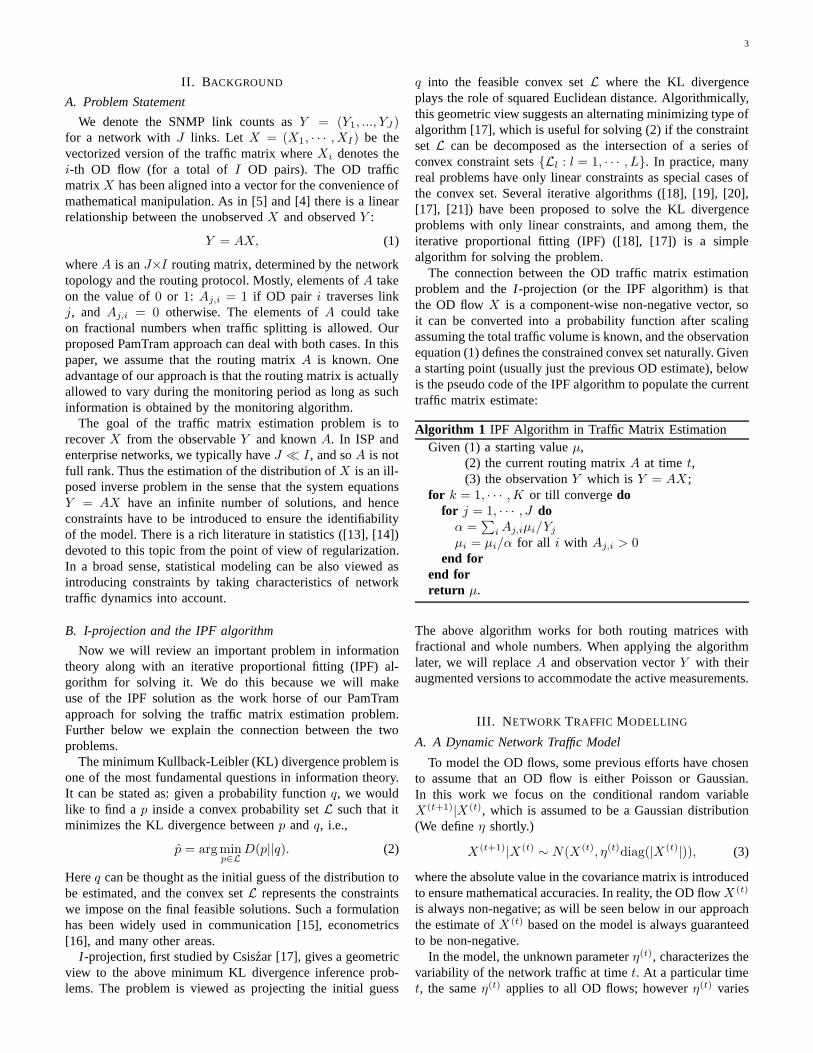
The connection between the OD traffic matrix estimationproblem and the I -projection (or the IPF algorithm) is thatthe OD flow X is a component-wise non-negative vector, soit can be converted into a probability function after scalingassuming the total traffic volume is known, and the observationequation (1) defines the constrained convex set naturally. Givena starting point (usually just the previous OD estimate), belowis the pseudo code of the IPF algorithm to populate the currenttraffic matrix estimate:

Algorithm 1 IPF Algorithm in Traffic Matrix EstimationGiven (1) a starting value µ,

(2) the current routing matrix A at time t,(3) the observation Y which is Y = AX ;

for k = 1, · · · , K or till converge dofor j = 1, · · · , J do

α =∑

i Aj,iµi/Yj

µi = µi/α for all i with Aj,i > 0end for

end forreturn µ.

The above algorithm works for both routing matrices withfractional and whole numbers. When applying the algorithmlater, we will replace A and observation vector Y with theiraugmented versions to accommodate the active measurements.

III. NETWORK TRAFFIC MODELLING

A. A Dynamic Network Traffic Model

To model the OD flows, some previous efforts have chosento assume that an OD flow is either Poisson or Gaussian.In this work we focus on the conditional random variableX(t+1)|X(t), which is assumed to be a Gaussian distribution(We define η shortly.)

X(t+1)|X(t) ∼ N(X(t), η(t)diag(|X(t)|)), (3)

where the absolute value in the covariance matrix is introducedto ensure mathematical accuracies. In reality, the OD flow X (t)

is always non-negative; as will be seen below in our approachthe estimate of X(t) based on the model is always guaranteedto be non-negative.

In the model, the unknown parameter η(t), characterizes thevariability of the network traffic at time t. At a particular timet, the same η(t) applies to all OD flows; however η(t) varies

4

vary over time and thus accounts for volatility of networktraffic. We assume that these parameters are bounded by aconstant η > 0, that is, η(t) < η. In short, our modelis spatially homogeneous but temporarily inhomogeneous.Empirical studies based on our dataset in Section V suggestthat η(t) usually takes on small values (Fig. 2 (c)).

We assume a linear mean-variance relationship on the condi-tional distribution of X(t+1) given X(t). In previous work, [4]and [11], a power-law mean-variance relationship (with linearas a special case) was used to model the marginal distributionof X(t). We make our assumption for two reasons. First, thislinear mean-variance relationship intuitively accounts for thephenomenon that large flows have large variations; we validatethis assumption later in Section V. Second, the network trafficis non-stationary. It is our intention to use the conditional rela-tionship, which essentially results in a non-stationary networktraffic model, to capture certain aspects of non-stationarity ofnetwork traffic and to track network dynamics.

Another important assumption of the model is that thecovariance matrix of this conditional distribution is diagonal,implying that all OD flows are independent. Intuitively, thereare few reasons for OD flows to be correlated as trafficsources and sinks are independent (such as independent endusers or web servers). Correlations can arise when some webservers are very popular, and thus many users send and receivepackets from the popular nodes. Similarly, OD flows that sharea source can be correlated. Incorporating such correlationswould lead to a block diagonal autocovariance matrix. Butany attempt to model such dependencies explicitly requiresadding a large number of parameters in the traffic model. Twoproblems can arise when attempting parameter estimation forsuch a model: a) we can end up fitting the noise instead ofthe true signals; and b) a large amount of data is needed to doparameter estimation. An in-depth exposition of this topic canbe found in [22]. We prefer to opt for a simple formulation, asspecified in (3), since simple models are always preferable aslong as they yield accurate estimates. The goal in modeling isto capture essential features of the traffic that lead to accurateestimates. A model need not incorporate all properties of thetraffic, if they are not essential to the estimate being sought.Our results show that the model we have chosen leads toestimates that are well below the 10% target.

One motivation for this conditional model is to introducea time series structure between consecutive time slots of anOD flow. This conditional model enables us to combine pasttraffic matrix estimates and the current link counts togetherto produce an estimate of a current traffic matrix. There aremany ways to incorporate previous estimates, such as usingit as an initial condition for an optimization procedure. Topopulate our traffic matrix we will use an estimate based onthe expectation of the current random variable conditionedupon the link constraints and the additional measurements weobtain, given the immediate previous estimate.

In this approach, the transitions of the traffic matrix fromone time interval to the next are controlled by the parameterη and small η’s imply that these transitions are not excessive.Clearly the validity of non-excessive transitions depends uponthe time scale the matrix intends to be used for. In our case,

we make estimates of a traffic matrix every 10 minutes. Ourmodel is intended to capture local behavior, that is, ”local” ina temporal sense (over a short window of time). We realizethat our model would not be an accurate description of trafficover long timescales such as many hours or days. However,our intent is to capture the transitional behavior of a trafficmatrix from one (short) interval to the next.

This modeling assumption has an alternate interpretationas a state-space model, which is used to describe internalunobservable states that evolve over time. The relationshipbetween the observable and unobservable variables is usuallyspecified as linear functionals typically with noise terms.In terms of state-space system notations, our model can berewritten as follows:

X(t+1) = X(t) +√

|X(t)|ε(t) (4a)

Y (t+1) = AX(t+1), (4b)

where the observable link traffic Y (t) ∈ RJ is a linearfunction of the unobservable OD traffic X (t) ∈ RI at timet. The routing matrix A, relating the unobservable states andobservations together, is a known sparse matrix (i.e., withmany zero entries). The errors ε(t) are identical independentdistributed normal random variables:

ε(t) ∼ N(0, η(t)), (5)

where, as discussed earlier, η(t) (< η) is an unknown parame-ter quantifying the dynamics of the underlying OD traffic. Wewould like to comment that there is no need to estimate η(t)’sin the OD estimation and flow selection. They are needed tocapture variability, however when computing a traffic matrixestimate using E(X |Y ), the actual Y ’s become fixed andthe η(t)’s cancel out. This will become clear in the proof ofTheorem 1 (see Appendix).

B. Error Metric

Before proceeding to our methods, we first introduce ourerror metric. It will be used as the objective in the optimizationproblem for estimating OD traffic, and will also assist in theselection of traffic flows to measure. We propose to use avariant of the mean square error (MSE) as the error metric toassess the performance of an estimator. Let X be an estimateof the unknown OD traffic X , then the MSE of X is definedas

MSE(X, X) = ||X − X ||2.

One drawback of the MSE metric is that it is not invariant tothe traffic volume changes. As our network traffic model isnon-stationary: the mean total traffic volume may increase ordecrease over time; hence, it is not reasonable to compareestimation performance at different time locations. Model(4) postulates that the variance is proportional to the mean(conditioned on the traffic in the previous time slot). Thisrelationship is used to devise the following scaled mean squareerror (sMSE) metric to mitigate the problem of MSE:

sMSE(X, X) =||X − X ||2

||X ||1=

∑

i(Xi − Xi)2

∑

i |Xi|.

5

Since we will use this sMSE metric for assessing perfor-mance, it is also used as our objective function in searchingfor the OD flow estimate. It is important to note that thescaling factor is a quantity that does not involve X ; hence,in effect, minimizing the sMSE is identical to minimizing theMSE metric.

Another justification of the sMSE metric is based on themodel we are using. Suppose at time t the true OD flow X (t)

were known and no link measurements were available, thenthe most sensible estimate for X (t+1) would be just X(t) itself.We can then calculate that the expected sMSE error under sucha scenario as

E(

sMSE(X(t), X(t+1)))

≈ η(t).

This indicates that if we start from the previous true OD flowX(t), the expected sMSE error will approximately be η(t),which quantifies the variability of the traffic according to ourmodel. So sMSE is meaningful to our model. In practice, ofcourse the previous true traffic is unknown to us, so two factorsare at play regarding the sMSE of the estimation. On one hand,we do not know X(t) but only its estimate X(t). On the otherhand, we can include (link or other extra active) measurementsto better the OD traffic estimation. The final expected errormetric will be influenced by both factors.

Other error metrics have been used in the past (e.g., [10]);a common one is the relative error defined as:

Rel-Error(Xi, Xi) =|Xi − Xi|

|Xi|.

It has been shown that in real networks, roughly 95% of thetotal load in the traffic matrix is carried by less than 1/2 or1/3 of the flows [9]. Moreover, the volume of flow in theseOD pairs can span several orders of magnitude. Hence, thereare typically very small traffic flows that generate extremelylarge relative errors and others are essentially irrelevant. Ourscaled MSE metric avoids this drawback, and works well as aperformance metric for both large and small flows. We pointout that in practice, the relative error is a useful measure tonetwork operators as it is intuitively appealing; thus we alsoreport on this metric in the results section.

IV. PARTIAL MEASUREMENT APPROACH

A. Incorporating Measurements

One of the central ideas in our method is that of couplingthe inference activity with the direct measurement of a smallnumber (possibly just one) of OD flow. To do this, it wouldbe necessary for flow monitors to be universally deployedthroughout a network. One might ask, if flow monitors aredeployed everywhere, why not just measure the traffic matrixentirely? In [2] the authors outline the overheads involved forboth centralized and distributed versions of full direct mea-surement. In both cases, the communications cost (informationbeing shipped to a central Network Operations location) re-mains very high. For these reasons, it is interesting to considermore lightweight uses of direct OD flow measurement.

A recent discovery illustrated that seemingly high dimen-sional network OD traffic actually resides in a space of much

lower dimensional [23]. This provides compelling intuition fora partial measurement approach, since it implies that thereis potential to learn a great deal about all the flows by onlymeasuring a few of them. In practice, it is challenging to get alow rank representation because the network traffic is volatile;hence, the representation changes over time. Our proposedpartial measurement approach is to use only a few activemeasurements to obtain some vital information to explorethis low dimensional space dynamically. We contend that theoriginal ill-posed problem becomes more well-posed even ifonly a tiny fraction of OD flows are measured directly at eachtime point, because the OD flows measured in recent time slotsremain informative due to temporal correlations in OD traffic.

The partial measurements can be incorporated into ourmodel as follows. Let M (t) be a k× I measurement matrix attime t. Each row of this matrix is a unit vector: it contains e′iif X

(t)i measured. We append M (t) to obtain the augmented

routing matrix A(t):

A(t) =

(

A

M (t)

)

.

Then the augmented observation vector Z(t) = A(t)X(t) isthe total observation available at time t. The first J entries inthis vector contain the link counts while any additional entriescontain the measured OD flows. In this paper, k, the rank ofM (t) is preset, i.e., the number of OD pairs to be measuredis determined. It is possible to treat it as a tuning parameterin different scenarios, however we find excellent performancewhen k = 1 and hence there is little motivation to exploreother values (at least for the dataset we study).

Equation 4b is now replaced so that our new systemequations, with the measurements incorporated, are given by

X(t+1) = X(t) +√

|X(t)|ε(t) (6a)

Z(t+1) = A(t)X(t+1). (6b)

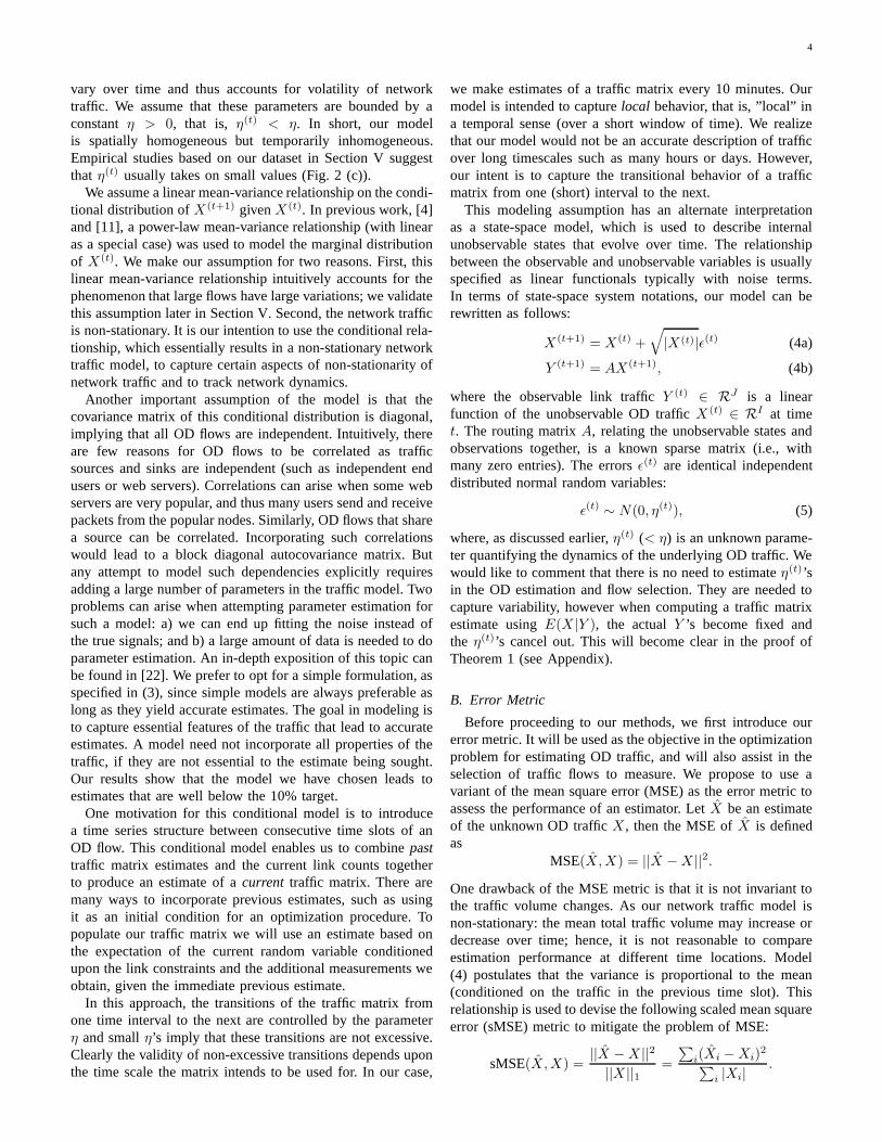
Our proposed PamTram approach is shown in Algorithm 2.The initial traffic matrix X(0) is set to be component-wisevector 1. This initial choice of traffic matrix is not veryimportant as the algorithm will quickly adjust itself to theright region. The first step is to measure a small set of wellselected OD flows using monitoring equipment. Step 2 of theprocedure corresponds to the usual optimization problem fortraffic matrix estimation, and many of the previous methodscould possibly be applied here. We will provide a fast im-plementation of an existing method. The challenge in Step 3is to determine which informative OD flows to measure. Wewill tackle these two questions separately in the following twosubsections.

Algorithm 2 Summary of the PamTram approach

Initialization: Set X0 = 1

for each time interval t do1. Measure OD pairs selected at step t − 1;2. Estimate X(t) based on data Z(1), · · · , Z(t)

3. Determine OD pairs to measure at t + 1.end for

6

In the following section, we will show that the IPF algorithmcan be used as an approximation method to solve the twooptimization problems (Step 2 and Step 3), that is both veryaccurate and very practical. It is practical because the imple-mentation of an IPF algorithm is much faster than indirectsolutions since it avoids matrix inversions (typically neededin Step 2), and integrating over long periods (typical in Step3).

The PamTram algorithm can be viewed as starting froma maximum entropy estimation in the following sense: afternormalization by the total OD traffic (which is naturally doneduring IPF), the OD traffic problem is equivalent to findingthe I -projection to the linear space of probability distributionsfrom a uniform distribution. This is intuitively appealingbecause a maximum entropy estimate implies that we startknowing nothing and thus need no prior knowledge. Henceour choice of initial traffic matrix X(0) is not important.

B. IPF and Minimum Mean Square Error Estimation

Now we state our workhorse algorithm, and its propertiesfor estimating OD traffic when both link traffic counts andsome direct measurement information are gathered (Step 2 inAlgorithm 2). This IPF algorithm was used first by Cao et. al.[4] as a post-processing step in their OD estimation algorithmbased on a Gaussian OD traffic model.

Since our goal is to be able to estimate the traffic matrix onthe timescale of minutes (e.g., 5 minutes for SNMP reporting,or 10 minutes as in our measurement) , we seek a fast onlinesolution. The IPF solution is an appealing option because: 1)it is easy to implement; 2) it converges in exponential rates(cf. Liang et. al. [12]), and is thus very fast in practice. TheIPF algorithm can be run satisfactorily in the order of O(IJ)with a preset finite number of iterations. The starting point attime t is determined by X(t−1), the estimate obtained fromthe previous step. It is reasonable to expect the starting valueto be in a small neighborhood of the OD traffic X (t) to beestimated; this further speeds up the convergence rate.

The following theorem justifies the use of IPF for theOD flow estimation under the dynamic traffic model from astatistical viewpoint.

Theorem 1: For the network dynamic model (4), condition-ing on X(t−1), if the mean vector µ (i.e., X (t−1)) is assumedknown, then the IPF estimate of X(t) is approximately theminimum MSE estimate.

The IPF algorithm was first proposed in [18]. in thecontext of fitting contingency tables with fixed margins. Itwas conjectured there that IPF approximately minimizes a(weighted) least square objective function (but there was noproof). [17] showed later that IPF minimizes actually the KL-divergence which is only an approximation to the (weighted)least square function as seen in the above theorem. Our proofis quite similar to the proof used in [1], but extends theirresult to a conditional Gaussian model. This theorem impliesthat the iterative proportional fitting (the I -projection estimate)approximately gives the minimum MSE estimate when µ =X(t−1) is known. In a real problem, X (t−1) is unknown hencereplaced by the previous estimate X(t−1). Another advantage

of the IPF algorithm that the resulting OD flow estimate ispositive, which is not guaranteed by the minimum MSE errorestimate.

Alternatively, the IPF algorithm can be justified as anapproximation to the true minimal MSE estimate given allpast observations. The true minimum MSE estimate of X (t)

is the conditional expectation of X (t) given all observations:

E(t) = E(

X(t)∣

∣

∣Z(1), · · · , Z(t)

)

.

The computation of such a quantity is very high: it involvesan integration over all past data points. To avoid this cost, wecan consider the following one-step approximation instead:

E(t) = E(

E(

X(t)|X(t−1), Z(t)) ∣

∣Z(1), · · ·Z(t))

≈ E(X(t)|X(t−1), Z(t)).(7)

This approximation is valid if the last parameter estimationX(t−1) is in the neighborhood of the true traffic X (t−1); thenthe IPF algorithm can be used to compute this conditionalexpectation approximately by starting from X(t−1).

C. Measurement Selection Scheme

1) Motivation: We now address the issue of how to selectthe OD flows to measure in each time interval (Step 3 inAlg. 2). The idea is to choose a scheme that will select themost informative of the unobservable flows. Clearly, the choicehas to be made based solely on the observable variables. Wefocus on selecting a single OD flow because even just measur-ing one OD flow per interval provides excellent performance.Our ideas here could be generalized to selecting a few flows,driving errors yet further down.

First, let us consider what an optimal solution would suggestand entail. Suppose X is a multivariate random variable (notnecessarily normal) with: E(X) = µ, and V ar(X) = Σ,where both µ and Σ are known (or can be estimated). Thenthe minimum MSE predictor for X is just µ with the MSEerror

E||X − µ||2 = trace(Σ).

Hence ideally, we would like to select an OD pair such that theresulting conditional covariance matrix given all observations

Σ(t) = Var(

X(t)∣

∣

∣Z(1), · · · , Z(t)

)

(8)

has the smallest trace. In other words, our task is to select theobservation matrix M (t) such that the trace of the conditionalvariance is minimized,

M (t) = arg minM(t)

traceΣ(t).

Intuitively this means we want to select the OD flows suchthat our estimation error was minimal. However, this approachis not attractive because the computation of Σ(t), involvingintegration over all past observations, is too costly.

Similarly to the approach for producing an approximationthat we mentioned in (7), we can also imagine using the sametype of approximation here for the conditional covariance in(8):

Var(

X(t)∣

∣

∣X(t−1) = X(t−1), Z(t)

)

7

However this remains difficult to compute because in general,for any random variables C and D, we have Var(C) =Var(E(C|D)) + E(Var(C|D)), that in our case translates to,

Var

(

E

(

X(t)

∣

∣

∣

∣

Z(t), X(t−1) = X(t−1)

)∣

∣

∣

∣

Z(1), · · · , Z(t)

)

.

which remains computationally difficult to approximate.2) Randomized Decision Rules: Since using Σ(t) to choose

the optimal OD flow to measure is too computationally in-tensive, we develop instead heuristic randomization schemesmotivated by game theory. Consider for a moment a uniformrandomization scheme in which, at each time step, each ODflow is selected for measurement with equal probability 1/I .The following theorem bounds the one-step error performance(the error made from one interval to the next) assuminguniform random sampling of flows.

Theorem 2: Let ω(t−1) be the sMSE error at step t − 1,

ω(t−1) = sMSE(

X(t−1), X(t−1))

.

Assume no link measurements Y are made, and only one ODpair is selected for measurement by uniform random sampling,then the expected value of ω(t), the error metric of X(t), isapproximately bounded by

E(ω(t)) ≤I − 1

Iω(t−1) + η(t) ≤

I − 1

Iω(t−1) + η,

where I is the number of total OD pairs. When t goes toinfinity, Iη is an upper bound of the expected error.

In the theorem, the expected value of the next step error met-ric is bounded by the sum of two parts: the first is the reductionin previous error thanks to the additional measurement; andthe second part (η) comes from the intrinsic variability (un-certainty) of the traffic itself. The theorem implies that when tgrows, the expected error will be bounded regardless of wherewe start.

This theorem is a comforting result in the sense that usinga uniform randomization scheme is not going to lead to anerror metric that can grow without bound. Since this casecorresponds to picking a flow arbitrarily, it can be viewedas a worst case bound. Indeed, as we will see, all of ouralternative randomization schemes produce smaller errors thanthe uniform randomization scheme.

In practice, link measurements Y (t) are obtained, so theresidual of the parameter estimate at time t is

R(t) = X(t) − E

(

X(t)

∣

∣

∣

∣

X(t−1) = X(t−1), Y (t)

)

. (9)

In order to reduce the sMSE (or equivalently the MSE),one should measure the OD pairs with the largest absoluteresidual(s). Note X(t−1) is only an estimate. We can view thetask of picking the OD flow with the largest residual as a twoperson game. One player is the traffic generator and the otheris the operator who is trying to guess the traffic volumes. Ateach move, the traffic generator changes the traffic volumes,and the operator’s move is to guess the traffic. We assumethat the traffic generator knows the strategy of the operatorand tries to select traffic volume levels so as to confuse the

operator as much as possible. Suppose the operator has a 0-1 loss function (the loss is 1 if it guesses correctly and 0otherwise). The operator’s goal is to maximize the probabilityof picking the largest residual, i.e.,

L(X(t−1), i) = 1

(

R(t)i = max

jR

(t)j

)

.

This corresponds to picking the largest random numberamongst a set, and hence we call our game a pick-largest-random-number game. The next theorem shows that randomguessing, i.e., the uniform randomization scheme above, is infact the minimax rule, and is thus the best option in this gamescenario.

Theorem 3: The uniform random sampling (p(i) = 1/I) isthe minimax decision rule of the pick-largest-random-numbergame with a 0-1 payoff (loss) function.

In reality, the ”traffic generator” player is not really anintelligent adversary. Although there is variability in traffic,there is also a good deal of temporal correlation, and manyflows vary slowly over short time scales. Hence, choosingOD pairs uniformly is likely to give poor results since theinformation in the previous traffic estimate is not exploited.In fact, since X(t−1) is likely to be close to the true trafficstate X(t−1), we should be able to guess reasonably well themoves of the traffic generator player, by relying on previousestimates. If we assume X (t−1) = X(t−1), then R(t) is a meanzero normal random variable with variance (independent ofY (t))

Λ(t) = Σ(t) − Σ(t)A′(AΣ(t)A′)−1AΣ(t), (10)

where Σ(t) = η(t)diag(X(t−1)), and the probability of R(t)i

being the largest residual in absolute value is

Q(i) = P

(

|R(t)i | = max

j|R

(t)j |

)

. (11)

In this alternate game, the operator now knows the strategyof the traffic generator in the sense that is has a model of thetraffic. A good strategy for the operator would be to pick anOD flow whose probability of generating the largest residual ishighest. Let Pmaxen(i) denote our strategy, i.e., the probabilityof picking flow i. We should choose Pmaxen(i) = Q(i) forthe following reason. If the operator has a negative log lossfunction, and the distribution Q is assumed to be known, thenit is well known that the solution that minimizes this lossfunction is given by the maximum entropy solution, i.e.,

Pmaxen = argminP

−∑

i

log P (i) log

(

Q(i)

P (i)

)

= Q.

Hence, we call this randomization scheme maxen.The uniform and maxen randomization schemes approach

the measurement selection from two opposing points of view.On one hand, the uniform scheme ignores the knowledge aboutthe network from previous time intervals. On the other hand,the maxen randomization scheme is based on the rationalethat the system changes slowly over time. Real networksexhibit both behaviors: sudden changes and sustained smoothtransitions. Hence we combine these two schemes to produce ascheme that sometimes allows departures from the base model.

8

Let α ∈ (0, 1). A weighted minimax randomization is definedas:

PwMaxen = αPuniform + (1 − α)Pmaxen.

Here we assume that the parameter α is preselected, and thatit could be tuned for particular networks. We usually set it asa relatively small number, such as 0.2, to favor the existingestimated models more.

3) Implementation of Decision Rules: For these random-ization schemes, the uniform is easy to realize, but theimplementation of the maxen randomization rule is difficultbecause the probabilities defined in (11) are hard to obtain.Instead of computing these probabilities explicitly, the maxenscheme can be implemented by generating multivariate normalrandom numbers whose covariance matrix is that specified in(10). Let µ = X(t−1), and X(t) ∼ N(µ, η(t)diag(µ)), then

X(t) − ΣA′(AΣA′)−1(AX(t) − Aµ) − µ (12)

is a mean zero multivariate normal random variable withcovariance matrix Λ(t). Our method is thus to use this distri-bution to generate I random numbers (recall I is the numberof OD flows), and then find the index of the largest one. But(12) requires the inversion of the matrix AΣ(t)A′, which iscomputationally expensive. Again, the result from Theorem 1shows that the IPF algorithm can be used to approximate

X(t) − ΣA′(AΣA′)−1(AX(t) − Aµ).

This can be solved approximately by using X (t) as a startingpoint and applying IPF to find a solution that fits the linkconstraint Y = Aµ. Thus a maxen randomization algorithmcan be devised as follows:

Algorithm 3 Maxen Randomization Algorithm

Let µ = X(t) and y = Aµ;1. Generate X ∼ N(µ, η(t)diag(µ));2. Project X onto {X |y = AX} to get X using IPF;3. Pick the jth OD flow if j = arg maxi |Xi − µi|.

Note that we needn’t be concerned about our choice for theparameter η(t) in this procedure. As mentioned earlier, duringthe computation of E(X |Y ), the η(t)’s cancel out (see proofof Theorem 1).

In summary, the total computational cost of PamTram is atmost the cost of executing IPF twice. If uniform sampling isused, we do not need Algorithm 3, and IPF will be executedonce. For the Maxen solution we use IPF twice. Since theIPF computation is light, we believe our solutions can scaleto larger networks.

D. Practical Issues of Flow Collection

There are some issues related to the practicality of ourproposed partial monitoring scheme. We realize that becausein practice the flow monitor is attached to a link, when we turnit on, we will in fact capture all the flows traversing that link.However, in this paper we study the case of measuring onlya single OD flow to understand the impact of this idea. Ourgoal is to understand, in general, how much flow measurement

is needed to obtain accurate traffic matrices. Since in practicewe have more than one OD flow, the errors will be lower thanwhat we calculate using only one OD flow.

The other practical problem is that when the flow monitorresides on a router, activating and deactivating flow mea-surements requires updating router configurations (e.g.,, onceevery 10 minutes). This could be viewed as high managementoverhead by network operators. There are two ways to avoidthis problem. First, it is possible to imagine alternate imple-mentation scenarios in which, for example, flow monitors areleft on all the time, and the results are either stored at themonitor or in a collection server residing in a PoP. Then thenetwork operations center could selectively pull flow records,a few at a time, as directed by our selection schemes.

A second option is to select the measurement schedule a fewhours in advance thus providing the network ample time todisseminate and schedule the monitoring activities, that couldbe loaded into monitors in batches. We consider a variation ofour randomization schemes is which the OD flows to measureare selected 24 hours in advance. The idea is that a flowselected for measurement at 2:10pm on one day, is actuallymeasured at 2:10pm the next day. The rational for such anapproach comes from both the observation of strong dailyperiodicity (as in Fig. 1) which shows that traffic is generallysimilar from one day to the next at a particular time of the day,and from [2] in which the authors illustrate this notion moreprecisely using fanouts. We call this a Latent scheme. Notea latent scheme is merely a scheduling approach that needsto be combined with a randomization rule. We evaluate bothLatent(maxen) and Latent(wMaxen).

V. EXPERIMENTAL ENVIRONMENT

A. The Data

Our data comes from Sprint’s European backbone that ismade up of 12 Points of Presence (PoPs) and 18 inter-PoPlinks. The network OD traffic information was collected byturning on Netflow (version 8) on all the Cisco routers. Thisversion of Netflow uses a sampling scheme of monitoring 1out of every 250 packets. The data was aggregated into PoPlevel flows at a time granularity of 10 minutes (i.e., averagenumber of bytes sent between PoP pairs during each 10 minutewindow). The data collection interval of 10 minutes waschosen to mitigate possible measurement errors. This is thesame dataset used in [8] hence some of our error statistics canbe directly compared to those in [8]. To avoid inconsistenciesbetween the link traffic and OD traffic, the link measurementdata are derived from the flow level measurements X ; thisguarantees that the traffic matrix X , the routing matrix A andthe link traffic counts Y are all in agreement with each other.This approach is well justified in [10].

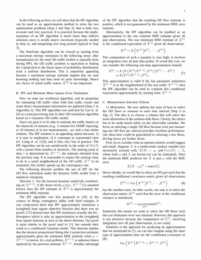
We now show some behaviors of this OD traffic data that,although they have been pointed out before, are includedhere for completeness. Fig. 1 shows two time series plotsof OD traffic flows selected because they represent commonbehaviors. 1 The first one shows strong periodicity (very

1The traffic volume has been multiplied by a randomly selected numberfor reasons of confidentiality.

9

Time

Tra

ffic

Vol

ume

050

010

00

0 500 1000 1500 2000 2500 3000

Sample Flow 1

200

300

400

0 500 1000 1500 2000 2500 3000

Sample Flow 2

Fig. 1. Two sample PoP level OD traffic flows.

common in OD pairs [23]). The strong periodicity of ODtraffic also induces strong periodicity in observed link traffic.The period of the traffic is exactly one day, while a weeklyperiod can also be seen over a longer time frame. Both samplesillustrate that sharp changes, different from the diurnal cyclesand from the local noise, can occur. These can occur forreasons such as router failures, the addition of new customers,or the removal of previous customers.

We now use this data to validate some of the assumptionsused in our model. The conditional linear mean-variancerelationship implies that we have

Ut,i =(

X(t)i − X

(t−1)i

)

/√

X(t−1)i ∼ N(0, η(t)).

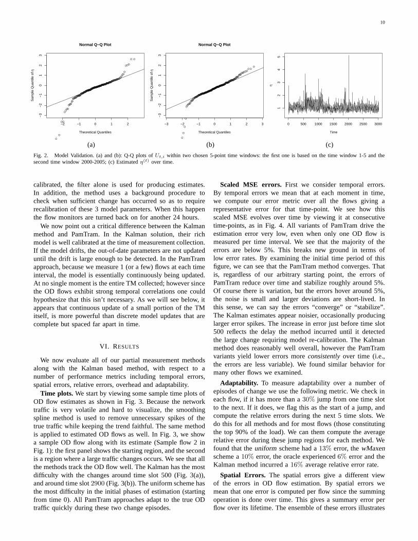
Even though η(t) varies over time, it is reasonable to assumethat it is continuous. Then we can estimate its value withineach small moving window. Fig. 2 shows two QQ-plots at twodifferent time points, and a time plot of the η(t) estimation. Weuse only the upper 90% of the traffic load to generate all threefigures, since we care less about faithfully representing thevery small flows than the larger ones constituting the majorityof the traffic. The Q-Q plots are produced based on all Ut,i

within a 50-minute window, i.e., 5 intervals. These two Q-Qplots are chosen because of their representativeness; data inother time windows show similar features. Fig. 2(a) is drawnbased on data points in the time window 1-5, and Fig. 2(b)is in time window 2000-2005, which is the region with thehighest spike (Fig. 2(c)). From both plots, we can see that theUt,i is very close to a normal distribution but with a longertail. Fig. 2 shows the estimated η(t) over time. Because Ut,i’shave a longer tail than normal, a robust estimate of η(t) basedon absolute moment ([24]) is used:

η(t) =

( ∑

i |Ut,i|

0.799× I

)2

,

where E(|V |) = 0.799 for V ∼ N(0, 1). From the plot,we can see that the values of η(t)’s mostly oscillate around1, which is very small given that a medium traffic flowmay take a value of several hundreds or thousands. Thereare occasional spikes in the figure – the most obvious onecorresponds to the sudden traffic changes occurring aroundtime slot 2000. Overall, the η(t) is well bounded except for

a few spike points. The plot shows that the conditional linearmean-variance relationship is a good approximation to the rawdata.

B. Partial Measurement Schemes

We tested PamTram using a number of partial measurementschemes to the Sprint PoP network data, including the uni-form, maxen, wMaxen, Latent(maxen), and Latent(wmaxen)schemes. For the wMaxen and Latent(wMaxen) versions,the weight parameter α is set as 0.2 to favor the maxenrandomization scheme. Our experiments show that the schemeis not very sensitive to the choice of α. In order to betterevaluate the performance of these randomization schemes,we also implemented an oracle scheme. The oracle has fullknowledge of the true OD traffic and thus the largest residualcan be precisely selected. In other words, we select the flowthat results in the smallest scaled MSE error in the nextparameter estimate. We can do this since we have the measuredtraffic matrix at our disposal. Although this cannot be done inpractice, it provides a means of assessing how far our schemesare from a sort of optimal (full knowledge) behavior. We havenot included the results for Latent(maxen) because they arevery similar to those of Latent(wMaxen) and due to lack ofspace. In almost all of our evaluations, we measure only oneOD flow in each 10 minute measurement interval.

C. Comparison to Kalman Filter method

We compare PamTram to the Kalman filter based methodthat was proposed in [25] and fully evaluated in [8]. Webriefly summarize the essential ideas here for completeness.We choose to compare our solution to the Kalman methodbecause that method resembles our solution in that it also usesa state space model coupled with partial flow measurements.

The state space model in the Kalman method is{

Xt+1 = CXt + Wt

Yt = AXt + Vt

(13)

where C is the state transition matrix, Wt is the dynamictraffic noise process and Vt is the measurement noise process.The diagonal elements of C capture temporal correlations forindividual OD flows, while the off diagonal elements of Ccapture spatial correlations across different OD flows. TheKalman filter is a two-step method that iterates each timeinterval. It first computes both a prediction for X at timet + 1 given all the data seen up to time t, namely Xt+1|t,and then computes a modified update when the new set oflink counts arrive at time t + 1, denoted Xt+1|t+1. This latterstep provides some of the adaptability of the Kalman methodbecause it estimates the TM using a model capturing temporaland spatial correlations, but modifies it to be in line with thelink counts.

To make these computations, the Kalman method needs tocalibrate the matrices C, ΣW and ΣV . To do this all the flowmonitors throughout a network are turned on for a period of24 hours. The 3 matrices are computed using this data viaan Expectation Maximization algorithm. Once the model is

10

−2 −1 0 1 2

−3

−2

−1

01

23

Normal Q−Q Plot

Theoretical Quantiles

Sam

ple

Qua

ntile

of η

−3 −2 −1 0 1 2 3

−3

−2

−1

01

23

Normal Q−Q Plot

Theoretical Quantiles

Sam

ple

Qua

ntile

of η

0 500 1000 1500 2000 2500 3000

12

34

5

Time

η

(a) (b) (c)

Fig. 2. Model Validation. (a) and (b): Q-Q plots of Ut,i within two chosen 5-point time windows: the first one is based on the time window 1-5 and thesecond time window 2000-2005; (c) Estimated η(t) over time.

calibrated, the filter alone is used for producing estimates.In addition, the method uses a background procedure tocheck when sufficient change has occurred so as to requirerecalibration of these 3 model parameters. When this happenthe flow monitors are turned back on for another 24 hours.

We now point out a critical difference between the Kalmanmethod and PamTram. In the Kalman solution, their richmodel is well calibrated at the time of measurement collection.If the model drifts, the out-of-date parameters are not updateduntil the drift is large enough to be detected. In the PamTramapproach, because we measure 1 (or a few) flows at each timeinterval, the model is essentially continuously being updated.At no single moment is the entire TM collected; however sincethe OD flows exhibit strong temporal correlations one couldhypothesize that this isn’t necessary. As we will see below, itappears that continuous update of a small portion of the TMitself, is more powerful than discrete model updates that arecomplete but spaced far apart in time.

VI. RESULTS

We now evaluate all of our partial measurement methodsalong with the Kalman based method, with respect to anumber of performance metrics including temporal errors,spatial errors, relative errors, overhead and adaptability.

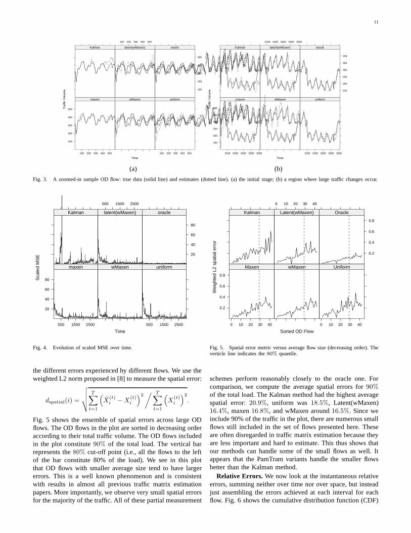
Time plots. We start by viewing some sample time plots ofOD flow estimates as shown in Fig. 3. Because the networktraffic is very volatile and hard to visualize, the smoothingspline method is used to remove unnecessary spikes of thetrue traffic while keeping the trend faithful. The same methodis applied to estimated OD flows as well. In Fig. 3, we showa sample OD flow along with its estimate (Sample flow 2 inFig. 1): the first panel shows the starting region, and the secondis a region where a large traffic changes occurs. We see that allthe methods track the OD flow well. The Kalman has the mostdifficulty with the changes around time slot 500 (Fig. 3(a)),and around time slot 2900 (Fig. 3(b)). The uniform scheme hasthe most difficulty in the initial phases of estimation (startingfrom time 0). All PamTram approaches adapt to the true ODtraffic quickly during these two change episodes.

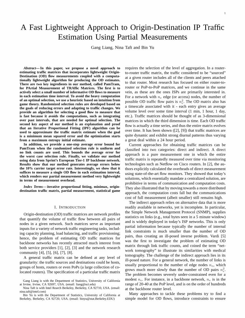
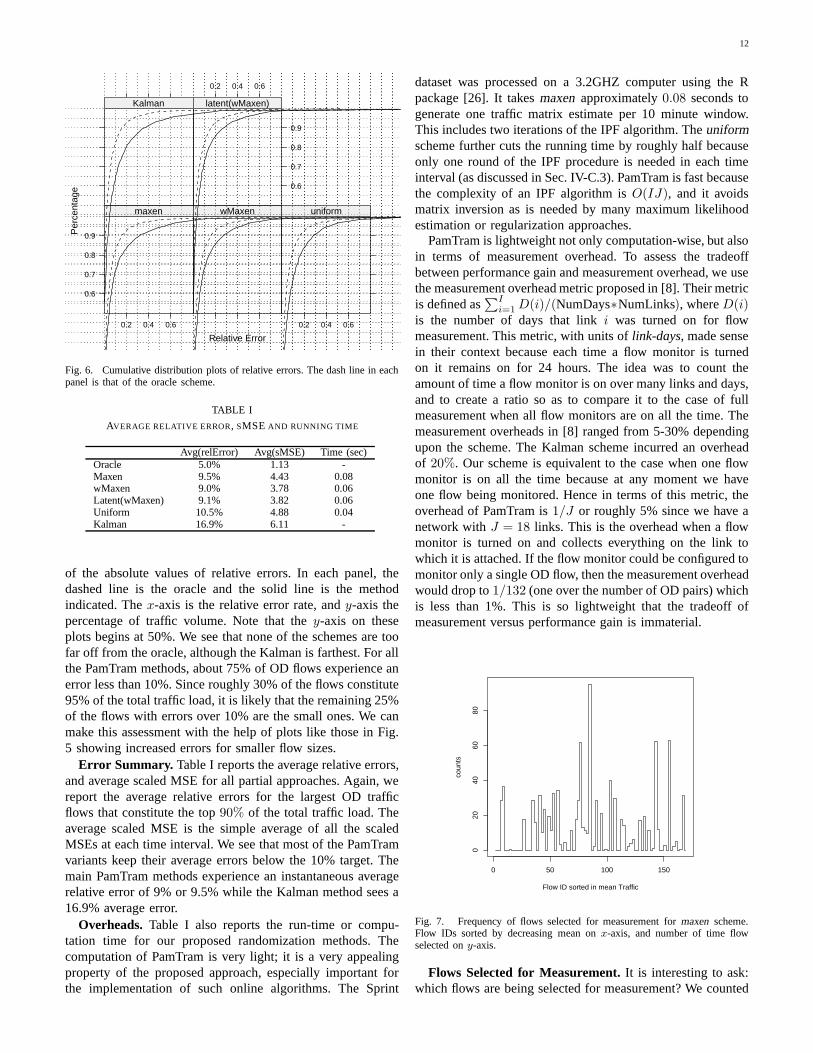
Scaled MSE errors. First we consider temporal errors.By temporal errors we mean that at each moment in time,we compute our error metric over all the flows giving arepresentative error for that time-point. We see how thisscaled MSE evolves over time by viewing it at consecutivetime-points, as in Fig. 4. All variants of PamTram drive theestimation error very low, even when only one OD flow ismeasured per time interval. We see that the majority of theerrors are below 5%. This breaks new ground in terms oflow error rates. By examining the initial time period of thisfigure, we can see that the PamTram method converges. Thatis, regardless of our arbitrary starting point, the errors ofPamTram reduce over time and stabilize roughly around 5%.Of course there is variation, but the errors hover around 5%,the noise is small and larger deviations are short-lived. Inthis sense, we can say the errors “converge” or “stabilize”.The Kalman estimates appear noisier, occasionally producinglarger error spikes. The increase in error just before time slot500 reflects the delay the method incurred until it detectedthe large change requiring model re-calibration. The Kalmanmethod does reasonably well overall, however the PamTramvariants yield lower errors more consistently over time (i.e.,the errors are less variable). We found similar behavior formany other flows we examined.

Adaptability. To measure adaptability over a number ofepisodes of change we use the following metric. We check ineach flow, if it has more than a 30% jump from one time slotto the next. If it does, we flag this as the start of a jump, andcompute the relative errors during the next 5 time slots. Wedo this for all methods and for most flows (those constitutingthe top 90% of the load). We can them compute the averagerelative error during these jump regions for each method. Wefound that the uniform scheme had a 13% error, the wMaxenscheme a 10% error, the oracle experienced 6% error and theKalman method incurred a 16% average relative error rate.

Spatial Errors. The spatial errors give a different viewof the errors in OD flow estimation. By spatial errors wemean that one error is computed per flow since the summingoperation is done over time. This gives a summary error perflow over its lifetime. The ensemble of these errors illustrates

11

Time

Tra

ffic

Vol

ume

100

200

300

400

500

100 200 300 400 500

maxen wMaxen

100 200 300 400 500

uniform

Kalman

100 200 300 400 500

latent(wMaxen)

100

200

300

400

500

oracle

Time

Tra

ffic

Vol

ume

150

200

250

300

350

400

2200 2400 2600 2800 3000

maxen wMaxen

2200 2400 2600 2800 3000

uniform

Kalman

2200 2400 2600 2800 3000

latent(wMaxen)

150

200

250

300

350

400

oracle

(a) (b)

Fig. 3. A zoomed-in sample OD flow: true data (solid line) and estimates (dotted line). (a) the initial stage; (b) a region where large traffic changes occur.

Time

Sca

led

MS

E

20

40

60

80

500 1500 2500

maxen wMaxen

500 1500 2500

uniform

Kalman

500 1500 2500

latent(wMaxen)

20

40

60

80

oracle

Fig. 4. Evolution of scaled MSE over time.

the different errors experienced by different flows. We use theweighted L2 norm proposed in [8] to measure the spatial error:

dspatial(i) =

√

√

√

√

T∑

t=1

(

X(t)i − X

(t)i

)2/ T∑

t=1

(

X(t)i

)2

.

Fig. 5 shows the ensemble of spatial errors across large ODflows. The OD flows in the plot are sorted in decreasing orderaccording to their total traffic volume. The OD flows includedin the plot constitute 90% of the total load. The vertical barrepresents the 80% cut-off point (i.e., all the flows to the leftof the bar constitute 80% of the load). We see in this plotthat OD flows with smaller average size tend to have largererrors. This is a well known phenomenon and is consistentwith results in almost all previous traffic matrix estimationpapers. More importantly, we observe very small spatial errorsfor the majority of the traffic. All of these partial measurement

Sorted OD Flow

Wei

ghte

d L2

spa

tial e

rror

0.2

0.4

0.6

0.8

0 10 20 30 40

Maxen wMaxen

0 10 20 30 40

Uniform

Kalman

0 10 20 30 40

Latent(wMaxen)

0.2

0.4

0.6

0.8

Oracle

Fig. 5. Spatial error metric versus average flow size (decreasing order). Theverticle line indicates the 80% quantile.

schemes perform reasonably closely to the oracle one. Forcomparison, we compute the average spatial errors for 90%of the total load. The Kalman method had the highest averagespatial error: 20.9%, uniform was 18.5%, Latent(wMaxen)16.4%, maxen 16.8%, and wMaxen around 16.5%. Since weinclude 90% of the traffic in the plot, there are numerous smallflows still included in the set of flows presented here. Theseare often disregarded in traffic matrix estimation because theyare less important and hard to estimate. This thus shows thatour methods can handle some of the small flows as well. Itappears that the PamTram variants handle the smaller flowsbetter than the Kalman method.

Relative Errors. We now look at the instantaneous relativeerrors, summing neither over time nor over space, but insteadjust assembling the errors achieved at each interval for eachflow. Fig. 6 shows the cumulative distribution function (CDF)

12

Relative Error

Per

cent

age

0.6

0.7

0.8

0.9

0.2 0.4 0.6

maxen wMaxen

0.2 0.4 0.6

uniform

Kalman

0.2 0.4 0.6

0.6

0.7

0.8

0.9

latent(wMaxen)

Fig. 6. Cumulative distribution plots of relative errors. The dash line in eachpanel is that of the oracle scheme.

TABLE I

AVERAGE RELATIVE ERROR, SMSE AND RUNNING TIME

Avg(relError) Avg(sMSE) Time (sec)Oracle 5.0% 1.13 -Maxen 9.5% 4.43 0.08wMaxen 9.0% 3.78 0.06Latent(wMaxen) 9.1% 3.82 0.06Uniform 10.5% 4.88 0.04Kalman 16.9% 6.11 -

of the absolute values of relative errors. In each panel, thedashed line is the oracle and the solid line is the methodindicated. The x-axis is the relative error rate, and y-axis thepercentage of traffic volume. Note that the y-axis on theseplots begins at 50%. We see that none of the schemes are toofar off from the oracle, although the Kalman is farthest. For allthe PamTram methods, about 75% of OD flows experience anerror less than 10%. Since roughly 30% of the flows constitute95% of the total traffic load, it is likely that the remaining 25%of the flows with errors over 10% are the small ones. We canmake this assessment with the help of plots like those in Fig.5 showing increased errors for smaller flow sizes.

Error Summary. Table I reports the average relative errors,and average scaled MSE for all partial approaches. Again, wereport the average relative errors for the largest OD trafficflows that constitute the top 90% of the total traffic load. Theaverage scaled MSE is the simple average of all the scaledMSEs at each time interval. We see that most of the PamTramvariants keep their average errors below the 10% target. Themain PamTram methods experience an instantaneous averagerelative error of 9% or 9.5% while the Kalman method sees a16.9% average error.

Overheads. Table I also reports the run-time or compu-tation time for our proposed randomization methods. Thecomputation of PamTram is very light; it is a very appealingproperty of the proposed approach, especially important forthe implementation of such online algorithms. The Sprint

dataset was processed on a 3.2GHZ computer using the Rpackage [26]. It takes maxen approximately 0.08 seconds togenerate one traffic matrix estimate per 10 minute window.This includes two iterations of the IPF algorithm. The uniformscheme further cuts the running time by roughly half becauseonly one round of the IPF procedure is needed in each timeinterval (as discussed in Sec. IV-C.3). PamTram is fast becausethe complexity of an IPF algorithm is O(IJ), and it avoidsmatrix inversion as is needed by many maximum likelihoodestimation or regularization approaches.

PamTram is lightweight not only computation-wise, but alsoin terms of measurement overhead. To assess the tradeoffbetween performance gain and measurement overhead, we usethe measurement overhead metric proposed in [8]. Their metricis defined as

∑I

i=1 D(i)/(NumDays∗NumLinks), where D(i)is the number of days that link i was turned on for flowmeasurement. This metric, with units of link-days, made sensein their context because each time a flow monitor is turnedon it remains on for 24 hours. The idea was to count theamount of time a flow monitor is on over many links and days,and to create a ratio so as to compare it to the case of fullmeasurement when all flow monitors are on all the time. Themeasurement overheads in [8] ranged from 5-30% dependingupon the scheme. The Kalman scheme incurred an overheadof 20%. Our scheme is equivalent to the case when one flowmonitor is on all the time because at any moment we haveone flow being monitored. Hence in terms of this metric, theoverhead of PamTram is 1/J or roughly 5% since we have anetwork with J = 18 links. This is the overhead when a flowmonitor is turned on and collects everything on the link towhich it is attached. If the flow monitor could be configured tomonitor only a single OD flow, then the measurement overheadwould drop to 1/132 (one over the number of OD pairs) whichis less than 1%. This is so lightweight that the tradeoff ofmeasurement versus performance gain is immaterial.

0 50 100 150

020

4060

80

Flow ID sorted in mean Traffic

coun

ts

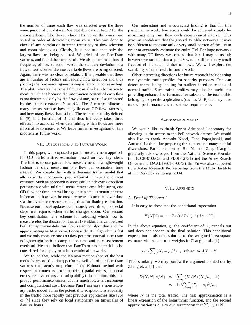
Fig. 7. Frequency of flows selected for measurement for maxen scheme.Flow IDs sorted by decreasing mean on x-axis, and number of time flowselected on y-axis.

Flows Selected for Measurement. It is interesting to ask:which flows are being selected for measurement? We counted

13

the number of times each flow was selected over the threeweek period of our dataset. We plot this data in Fig. 7 for themaxen scheme. The flows, whose IDs are on the x-axis, aresorted in order of decreasing mean value. This was done tocheck if any correlation between frequency of flow selectionand mean size exists. Clearly, it is not true that only thelargest flows are being selected. We tried this on PamTramvariants, and found the same result. We also examined plots offrequency of flow selection versus the standard deviation of aflow to test whether the most variable flows are being selected.Again, there was no clear correlation. It is possible that thereare a number of factors influencing flow selection and thusplotting the frequency against a single factor is not revealing.The plot indicates that small flows can also be informative tomeasure. This is because the information content of each flowis not determined only by the flow volume, but is also impactedby the linear constraints Y = AX . The A matrix influencesmany factors, such as how many links an OD flow traverses,and how many flows share a link. The residual quantity definedin (9) is a function of A and thus indirectly takes theseeffects into account, when determining which flows are moreinformative to measure. We leave further investigation of thisproblem as future work.

VII. DISCUSSIONS AND FUTURE WORK

In this paper, we proposed a partial measurement approachfor OD traffic matrix estimation based on two key ideas.The first is to use partial flow measurement in a lightweightfashion by only measuring one flow per estimation timeinterval. We couple this with a dynamic traffic model thatallows us to incorporate past information into the currentestimate. Such an approach is successful in achieving excellentperformance with minimal measurement cost. Measuring oneOD flow per time interval brings only a small amount of extrainformation; however the measurements accumulate over timevia the dynamic network model, thus facilitating estimation.Because our model updates continuously over time, no specialsteps are required when traffic changes occur. Our secondkey contribution is a scheme for selecting which flow tomeasure plus the illustration that an IPF algorithm can be usedboth for approximately this flow selection algorithm and forapproximating an MSE error. Because the IPF algorithm is fastand we only measure one OD flow per time interval, PamTramis lightweight both in computation time and in measurementoverhead. We thus believe that PamTram has potential to beconsidered for deployment in operational networks.

We found that, while the Kalman method (one of the bestmethods proposed to date) performs well, all of our PamTramvariants consistently outperformed the Kalman method withrespect to numerous errors metrics (spatial errors, temporalerrors, relative errors and adaptability). In addition, this im-proved performance comes with a much lower measurementand computational cost. Because PamTram uses a nonstation-ary traffic model, it has the potential to adapt to nonstationarityin the traffic more rapidly that previous approaches like [25]or [4] since they rely on local stationarity on timescales ofdays or hours.

Our interesting and encouraging finding is that for thisparticular network, low errors could be achieved simply bymeasuring only one flow each measurement interval. Thisgives us confidence that for general ISP-like networks, it maybe sufficient to measure only a very small portion of the TM inorder to accurately estimate the entire TM. For large networkswith many OD flows, we contend that k > 1 may be useful;however we suspect that a good k would still be a very smallfraction of the total number of flows. We will explore thescalability of this result in future work.

Other interesting directions for future research include usingour dynamic traffic profiles for security purposes. One candetect anomalies by looking for outliers based on models ofnormal traffic. Such traffic profiles may also be useful forproviding enhanced performance for subsets of the total trafficbelonging to specific applications (such as VoIP) that may haveits own performance and robustness requirements.

ACKNOWLEDGMENTS

We would like to thank Sprint Advanced Laboratory forallowing us the access to the PoP network dataset. We wouldalso like to thank Antonio Nucci, Dina Papagianaki, andAnukool Lakhina for preparing the dataset and many helpfuldiscussions. Partial support to Bin Yu and Gang Liang isgratefully acknowledged from the National Science Founda-tion (CCR-0106656 and FD01-12731) and the Army RearchOffice grant (DAAD19-01-1-0643). Bin Yu was also supportedby a Miller Research Professorship from the Miller Instituteat UC Berkeley in Spring, 2004.

VIII. APPENDIX

A. Proof of Theorem 1

It is easy to show that the conditional expectation

E(X |Y ) = µ − ΣA′(AΣA′)−1(Aµ − Y ).

In the above equation, η, the coefficient of A, cancels outand does not appear in the final solution. This conditionalexpectation is also the solution to the weighted least-squareestimate with square root weights in Zhang et. al.. [1]

min∑

i(Xi − µi)

2/µi subject to AX = Y.

Then similarly, we may borrow the argument pointed out byZhang et. al.[1] that

D(X/N ||µ/N) ≈∑

i(Xi/N) (Xi/µi − 1)

≈ 1/N∑

i(Xi − µi)

2/µi,

where N is the total traffic. The first approximation is alinear expansion of the logarithmic function, and the secondapproximation is due to our assumption that

∑

i µi ≈ N .

14

B. Proof of Theorem 2

Let K denote the index of the OD pair to be measured;hence, we have P (K = k) = 1/I . Under the assumption thatno any link measurement is obtained, we have

X(t)k =

{

X(t)k if K = k

X(t−1)k otherwise.

Similarly, we define X(t+1) as

X(t)k =

{

X(t)k if K = k

X(t−1)k otherwise,

which is the parameter estimate if we start from the true value.Fix X(t−1) and X(t−1) at first, then the expected value of

the scaled MSE is

E

(

||X(t) − X(t)||2∑

i X(t)i

)

≈E||X(t) − X(t)||2∑

i X(t−1)i

=E||X(t) − X(t)||2 + E||X(t) − X(t)||2

∑

i X(t−1)i

(14)

The first approximation is obtained by the delta method [24],and the second equality holds because

E(

||(X(t) − X(t)) + (X(t) − X(t))||2)

= E

(

E

(

||(X(t) − X(t)) + (X(t) − X(t))||2∣

∣

∣

∣

K =k, X(t)k

))

.

Note given K =k and X(t)k , X(t) − X(t) are determined, and

X(t) −X(t) is a mean 0 multivariate normal random variable.The cross terms disappear after expanding the square term.

For each term in (14), we have

E||X(t) − X(t)||2∑

i X(t−1)i

=||X(t) − X(t)||2 −

∑

k P (k)(X(t−1)k − X

(t−1)k )2

∑

i X(t−1)i

≤I − 1

Iω(t−1),

andE||X(t) − X(t)||2∑

i X(t−1)i

≤ η.

So in summary, we have

E(ω(t)) ≤I − 1

Iω(t−1) + η(t) ≤

I − 1

Iω(t−1) + η.

Note that the above bound actually does not depend on thevalue of X(t), implying the inequality holds generally.

Let γ(t) = E(

ω(t))

. Taking an expectation over both sidesof the above inequality, we have

γ(t) ≤I − 1

Iγ(t−1) + η. (15)

Based on the above inequality, we can easily get the inequality:

γ(t) ≤ at−1γ(0) +1 − at−1

1 − aη ≤ at−1γ(0) + Iη,

where a = 1 − 1/I and γ(0) is the initial error. As t tends toinfinity, at−1 tends to zero so asymptotically the influence ofγ(0) diminishes exponentially. It implies that Iη is the upperbound of the expected error metric in the long run.

C. Proof of Theorem 3

If only we can show that the uniform selection rule P (i) =1/I is an equalizer decision rule. First note that

EP

(

L(R(t), i))

= 1/I,

independent of the distribution of R(t) as long as the i ischosen independent of R(t). It implies that the such a decisionrule is actually an equalizer for the game:

Ep

(

maxX(t−1)

L(R(t), i)

)

= 1/I.

So the uniform rule is minimax.

REFERENCES

[1] Y. Zhang, M. Roughan, C. Lund, and D. Donoho, “An information-theoretic approach to traffic matrix estimation,” in ACM SIGCOMM,2003.

[2] K. Papagiannaki, N. Taft, and A. Lakhina, “A distributed approach tomeasure ip traffic matrices”,” in ACM Internet Measurement Conference,October 2004.

[3] A. Gunnar, M. Johansson, and T. Telkamp, “Traffic matrix estimationon a large ip backbone - a study on real data,” in Proc. ACM IMC,October 2004.

[4] J. Cao, D. Davis, S. V. Wiel, and B. Yu, “Time-varying network to-mography: router link data,” Journal of American Statistics Association,vol. 95, pp. 1063–1075, 2000.

[5] Y. Vardi, “Network tomography: Estimating source-destination traffic in-tensities from link data,” Journal of the American Statistical Association,vol. 91, pp. 365–377, 1996.

[6] S. Vaton and A. Gravey, “Network tomography : an iterative bayesiananalysis,” in Proc. ITC 18, August 2003.

[7] G. Liang and B. Yu, “Pseudo likelihood estimation in network tomog-raphy,” in IEEE Infocom 2003, San Francisco, April 2003.

[8] A. Soule, A. Lakhina, N. Taft, K. Papagiannaki, K. Salamatian, A. Nucci,M. Crovella, and C. Diot, “Traffice matrices: Balancing measurement,modeling and inference,” in ACM Sigmetrics, June 2005.

[9] A. Soule, A. Nucci, E. Leonardi, R. Cruz, and N. Taft, “How toidentify and estimate the largest traffic matrix elements in a dynamicenvironment,” in ACM Sigmetrics, June 2004.

[10] Y. Zhang, M. Roughan, N. Duffield, and A. Greenberg, “Fast accuratecomputation of large-scale ip traffic matrices from link loads,” in ACMSigmetrics, San Diego, USA, June 2003.

[11] G. Liang and B. Yu, “Maximum pseudo-likelihood estimation in networktomography,” IEEE Transactions on Signal Processing, vol. 51, no. 8,pp. 2043–2053, August 2003.

[12] G. Liang, B. Yu, and N. Taft, “Maximum entorpy models: convergencerates and application in dynamic system monitoring.” in InternationalSymposium on Information Theory, 2004.

[13] M. Hanke and P. Hansen, “Regularization methods for large-scaleproblems,” Surveys on Mathematics for industry, vol. 3, pp. 253–315,1993.

[14] G. Wahba, “Spline models for observational data,” in SIAM, Philadel-phia, 1990.

[15] C. Shannon, “A mathematical theory of communication,” Bell SystemTechnical Journal, vol. 27, no. 3, pp. 623–656, July, Oct 1948.

[16] R. McDougall, “Entropy theory and ras are friends,” Center for GlobalTrade Analysis, Department of Agricultural Economics, Purdue Univer-sity, GTAP Working Papers 300, 1999.

[17] I. Csiszar, “I -divergence geometry of probability distributions and min-imization problems.” The Annals of Probability, vol. 3(1), pp. 146–158,1975.

[18] W. Deming and F. Stephan, “On a least square adjustment of a sampledfrequency table when the expected marginal totals are known,” Ann.Math. Statist., no. 11, pp. 427–444, 1940.

15

[19] J. Darroch and D. Ratcliff, “Generalized iterative scaling for log-linearmodels,” The Annals of Mathematical Statistics, vol. 43, no. 5, pp. 1470–1480, 1972.

[20] S. D. Pietra, V. D. Pietra, and J. Lafferty, “Induce features of randomfields,” IEEE Transaction on Pattern Analysis and Machine Intelligence,vol. 19, no. 4, pp. 380–393, 1997.

[21] M. Schneider and S. Zenios, “A comparative study of algorithms formatrix balancing,” Operational Research, vol. 38, no. 3, pp. 439–455,1990.

[22] P. Bickel and E. Levina, “Some theory for Fisher’s linear discriminantfunction, ‘naive bayes’, and some alternatives when there are many morevariables than observations,” Bernoulli, vol. 10, no. 6, p. 9891010, 2004.

[23] A. Lakhina, K. Papagiannaki, M. Crovella, C. Diot, E. Kolaczyk,and N. Taft, “Structural analysis of network traffic flows,” in ACMSigmetrics, June 2004.

[24] J. Rice, Mathematical Statistics and Data Analysis. Duxbury Press,1988.

[25] A. Soule, K. Salamatian, and N. Taft, “Traffic matrix tracking usingkalman filters,” Large Scale Network Inference Workshop at ACMSigmetrics, June 2005.

[26] R. Ihaka and R. Gentleman, “R: A language for data analysis andgraphics,” Journal of Computational and Graphical Statistics, vol. 5,no. 3, pp. 299–314, 1996.

Gang Liang Gang Liang received the B.S. andM.S. degree in statistics from Peking Universityin 1996 and 1999, and the Ph.D. degree from theUniversity of California at Berkeley in 2004. Heis now an assistant professor in the Department ofStatisics, University of Californina at Irvine. Hisresearch interests span several fields including statis-tical problems on data network, information theory,algorithm development, and machine learning.

Nina Taft Nina Taft received the B.S degree incomputer science from the University of Pennsyl-vania in 1985, and the M.S. and Ph.D. degreesfrom the University of California at Berkeley in1990 and 1994, respectively. From 1995 to 1999,she was a researcher at SRI International in MenloPark, CA, working on congestion control and routingin ATM networks. From 1999 to 2003, she wassenior researcher at Sprint?s Advanced Technol-ogy Laboratories working on Internet measurement,modeling and performance evaluation. She joined

Intel Research in Berkeley, CA in September of 2003. Her research interestsare in traffic modeling, traffic generation methods, distributed monitoring andnetwork security.

Bin Yu Bin Yu is Professor of Statistics at Uni-versity of California at Berkeley. She also holds aChangJiang Chair Professorship at Peking Univer-sity, and is the founding co-director of the MicrosoftLab on Statistics and Information Technology atPeking University. Her current research interestsinclude machine learning, information theory, andstatistical problems from remote sensing, internettomography, sensor networks, neuroscience, finance,and bioinformatics.

She was in the S.S. Chern exchange programbetween China and US, and obtained her B.S. from Peking University andM.A. and PhD from University of California at Berkeley. She was a regularor visiting faculty at University of Wisconsin at Madison, Yale University,MIT and ETH (Zurich). She was a Member of Technical Staff at Lucent BellLabs from 1998-2000 and holds two U.S. patents.

She is a Fellow of IEEE and IMS (Inst of Math. Stats) and ASA (AmericanStatistical Association), was a Special Inviated (now Medallion) Lecturer ofIMS in 1999, and a Miller Research Professor at Berkeley in spring 2004.She has served and is serving on many editorial boards including the Annalsof Statistics, J. Amer. Statist. Assoc. and J. Machine Learning Research. Shewas a guest co-editor for Statistica Sinica on Bioinformatics and for IEEESignal Processing on Machine Learning, and a co-editor of a Springer bookon Nonlinear regression and classification. She was elected to the council ofIMS (one term) and IEEE Information Theory Society (two terms).