Embed Size (px)
Citation preview

sustainable urban transport development
a dynamic optimisation approach

Dissertation committee:
prof. dr. ir. H. J. Grootenboer University of Twente, chairman/secretaryprof. dr. ir. M. F. A.M. van Maarseveen University of Twente, promotorprof. dr. E.O. Akinyemi University of Ilorin, Nigeria, promotorprof. dr. ir. B. van Arem University of Twenteprof. dr. ir. E.C. van Berkum University of Twenteprof. dr. G. P.M.R. Dewulf University of Twenteprof. dr.-ing. H. Knoflacher Vienna University of Technology, Austriadr. S. P. Shepherd University of Leeds, United Kingdom
Trail Thesis Series T2005/3, The Netherlands TRAIL Research SchoolThis thesis is the result of a Ph.D. study carried out between 1999 and 2005 atthe University of Twente, faculty of Engineering Technology, department of CivilEngineering, Centre for Transport Studies.
Cover picture: Detail of rickshaw and taxis in a Kolkata street, IndiaCopyright c© by Bennett Dean/Eye Ubiquitous/Corbis/TCS
Typeset in LATEX
Copyright c© 2005 by M.H.P. Zuidgeest, Enschede, The Netherlands
All rights reserved. No part of this publication may be reproduced, stored in a
retrieval system, or transmitted, in any form or by any means, electronic, mechanical,
photocopying, recording or otherwise, without the written permission of the author.
Printed by Febodruk BV, Enschede, The Netherlands.
ISBN 90-365-2174-2

sustainable urban transport development
a dynamic optimisation approach
PROEFSCHRIFT
ter verkrijging vande graad van doctor aan de Universiteit Twente,
op gezag van de Rector Magnificus,prof. dr. W.H.M. Zijm,
volgens besluit van het College voor Promotiesin het openbaar te verdedigen
op donderdag 28 april 2005 om 16.45 uur
door
Marcus Henricus Petrus Zuidgeest
geboren op 23 januari 1974te Den Helder

Dit proefschrift is goedgekeurd door de promotoren:
prof. dr. ir. M. F. A. M. van Maarseveenprof. dr. E. O. Akinyemi

“It is twenty-five kilometres from Addis Ababa to theSabeta waterfall. Driving a car in Ethiopia is a kindof unending process of compromise: everyone knowsthat the road is narrow, old, crammed with people andvehicles, but they also know that they must somehowfind a spot for themselves on it, and not only find aspot, but actually move, advance forward, make theirway toward their destination. Every few moments, eachdriver, cattle herder, or pedestrian is confronted by anobstacle, a conundrum, a problem that needs solving:how to pass without colliding with the car approachingfrom the opposite direction; how to hurry along one’scows, sheep, and camels without trampling the childrenand crawling beggars; how to cross without getting runover by a truck, being impaled on the horns of a bull,knocking over that woman carrying a twenty-kilogramweight on her head. And yet no one shouts at any-one else, no one falls into a fury, no one curses orthreatens-patiently and silently, they all perform theirslalom, execute their pirouettes, dodge and evade, ma-neuver and hedge, turn here, converge there, and, mostimportant, move forward.”
Ryszard KapuscinskiThe Shadow of the Sun: my African life.


Preface
In my opinion, Ryszard Kapuscinski’s observations on driving a car in Ethiopia(page v) very well symbolise the process of a Ph.D. research. As a matter offact, the same observations also perfectly stand for my personal motivation tostart a research in modelling sustainable transport, back in 1999, in the firstplace.
When I was walking in a tropical city for the first time in my life, that wasin Guatemala-City in 1995, its traffic fascinated me very much. Busyness andnoise. Chaotic traffic, but still structured and often very efficient. Understan-ding, describing and modelling this apparent chaos, that would be the topicof my research! In the end, everything turned out to be different, and thisresearch got a more general character. Still, I hope this work motivates manypeople to continue research in the interesting and important field of transportsustainability.
In a traffic flow you are never alone, hence I would like to mention and thanksome people who, sometimes literally, travelled along with me.
First and foremost, I am indebted to my supervisors, Prof. Dr. Martin vanMaarseveen and Prof. Dr. Edward Akinyemi, who provided the necessary (in-tellectual) infrastructure and means to do research. Eddie, your qualities andqualifications are often underestimated, I am proud to say I did my Ph.D. withyou. Thank you for all your valuable lessons (in life). Martin, in the famousHotel le Benin in Lome some dodgy characters thought you were my father.Our conversations were indeed often very personal, almost family like, whereyou showed great insight in human nature. Thank you for the confidence inme.
In the early stages of the dynamic modelling, I had the privilege and pleasureto work with Dr. Clifford Wymer, former econometrist with the InternationalMonetary Fund. Clifford, your enthusiasm for continuous-time macro-economicmodelling and your never-ending patience with me are least-to-say unique.Thank you very much. Also the hospitality I received in London while stayingwith you and your wife Jill are unforgettable. It is a pity I had to move awayfrom using your software in the end.
vii

viii
The discussions I had with Dr. Kieran Donaghy from the University of Illinoisat Urbana-Champaign, USA, and Dr. Laurie Schintler from George MasonUniversity, USA, during a workshop in Bonn and by e-mail were very usefulfor better understanding of their interesting model. Thank you very much.
My colleagues in the UT department of mathematical systems and controltheory helped me a lot, especially with respect to mathematical notations. Inparticular, I wish to acknowledge Dr. Bram van den Broek.
I would also like to thank the members of the dissertation committee for readingthe thesis and giving me their criticisms and suggestions.
During my research visit to the National Center for Transportation Studies,University of the Philippines Diliman in Manila, I received great hospitalityand help, in particular by Dr. Noriel Tiglao, Dr. Jose Regidor, Mr. Ed Kamid,Ms. Alorna Abao and Dr. Ricardo Sigua. Furthermore, in the Asian Develop-ment Bank I was kindly received by Mr. Herbert Fabian and Mr. Cornie Hui-zenga. In addition, I would like to thank my colleagues and students in ITC,in particular Mr. Rizal Cruz, Mr. Javier Pacheco, Mr. Sherif Amer, Mr. Johande Meijere as well as Dr. Luc Boerboom, who helped me a lot in organising thefield visits to Malaysia and The Philippines.
The contributions of some of my former M.Sc. students who tackled interes-ting problems in the field of sustainable transport that were of direct or indirectimportance to this thesis are also greatly acknowledged. In particular I wouldlike to mention the researches of Mr. Thijs Oude Moleman on sustainabilityindicators, Mr. Manus Barten on optimisation in transport planning (partlyreported in chapter 4), Mr. Alex van Gent on transport network aggregati-on, Ms. Annette van Nes on environmental capacity, Mr. Roland Kager ontransport modelling in developing countries and Mr. Martijn Bierman on theexistence and measurement of elastic demand in Metro Manila.
Also thanks to (former) colleagues and friends from within the UT faculty ofEngineering Technology, in particular to Giovanni (for keeping me companyduring weekend and evening shifts), Peter & Mako (for the many dinners andlong evenings in cafe Bolwerk), Bas & Roland (for putting things in perspec-tive with their Centre of Irrelevance), Frans & Kasper (for stepping in withVerkeer as well as being great colleagues), Bart (2×), Martin, Eric, Henny,Wendy, Thijs, Cornelie, Mascha, Cees, Michiel, Jean-Luc, Jebbe, Godfried,Attila, Pieter, Jorg, Caroline, Jan-Willem, Wilbert, Astrid, Marjolein, Suzan-ne, Leo, Marc (for reviewing chapter 4), Maureen, Dorette, Harry, Henriette,Graziana, Hans, Sam, Matthijs, Anne, Rene, Judith, Anne-Marie, Lynn, Rien,Denie, and Martijn (2×), who make that I still enjoy working here.
My former colleagues and students in UNESCO-IHE-Delft have introduced meto so many interesting topics as well as cultures. In particular, many thanks goto Mr. Jan Herman Koster, who kept on believing in me, even after I decided

ix
to leave for Twente.
My (former) colleagues in Keypoint Consultancy, in particular Mr. Leo deJong, Dr. Marc Witbreuk and Mr. Lars Mosch, who made that once in a whileI could focus on the practical side of traffic and transport by reviewing theirconsultancy reports. Thanks for the trust in me!
On a personal note, no one can get by without help of friends and family.Too many persons to mention individually, I wish to say: ‘groep Utrecht’,‘campusmongolen’, dear family(-in-law) and study-friends, Thanks! Bart andPeter, thank you very much for being paranymphs during my defence. Yourfriendship and help throughout the last five years are very much appreciated.
Finally, I would like to thank Cari, who, even when I seemed to walk aroundin a fog at times, stayed confident and optimistic. Cari, without your love andcare this work would probably never have finished.
mz


Contents
Preface vii
I Sustainable urban transport development 1
1 Introduction 31.1 Transport realities . . . . . . . . . . . . . . . . . . . . . . . . . 31.2 Transport planning . . . . . . . . . . . . . . . . . . . . . . . . . 8
1.2.1 Supply and demand . . . . . . . . . . . . . . . . . . . . 91.2.2 Transport modelling . . . . . . . . . . . . . . . . . . . . 121.2.3 Transport modelling alternatives . . . . . . . . . . . . . 22
1.3 Strategic transport planning . . . . . . . . . . . . . . . . . . . . 241.4 Problem statement and research questions . . . . . . . . . . . . 271.5 Limitations of this research . . . . . . . . . . . . . . . . . . . . 291.6 Scope and outline of this thesis . . . . . . . . . . . . . . . . . . 29
2 Sustainable development and transport 312.1 The Limits to Growth . . . . . . . . . . . . . . . . . . . . . . . 312.2 Sustainability and sustainable development . . . . . . . . . . . 35
2.2.1 Three conceptions of sustainable development . . . . . . 372.2.2 Three dimensions of sustainable development . . . . . . 392.2.3 Three levels of discourse . . . . . . . . . . . . . . . . . . 402.2.4 Sustainable urban development . . . . . . . . . . . . . . 41
2.3 Sustainable urban transport development . . . . . . . . . . . . 432.3.1 A framework for sustainable transport development . . 452.3.2 A different transport planning paradigm . . . . . . . . . 49
3 Sustainable transport development requirements 533.1 Introduction . . . . . . . . . . . . . . . . . . . . . . . . . . . . . 533.2 Movement needs and transport system performance . . . . . . 53
3.2.1 Level-of-Service . . . . . . . . . . . . . . . . . . . . . . . 553.2.2 Mobility and person travel . . . . . . . . . . . . . . . . . 553.2.3 Accessibility . . . . . . . . . . . . . . . . . . . . . . . . . 573.2.4 Equity . . . . . . . . . . . . . . . . . . . . . . . . . . . . 61
3.3 Transport and development . . . . . . . . . . . . . . . . . . . . 63
xi

xii CONTENTS
3.3.1 Dynamics in travel demand . . . . . . . . . . . . . . . . 653.4 Resource consumption and capacities . . . . . . . . . . . . . . . 70
3.4.1 Measures for controlling transition paths . . . . . . . . . 74
II Modelling sustainable transport development 77
4 Optimisation as a tool for sustainable transport policy design 794.1 Transport policy and planning . . . . . . . . . . . . . . . . . . 79
4.1.1 The transport policy process . . . . . . . . . . . . . . . 794.1.2 Decision-making approaches . . . . . . . . . . . . . . . . 814.1.3 Complex transport policy objectives . . . . . . . . . . . 82
4.2 Transport planning as a design problem . . . . . . . . . . . . . 834.2.1 Existing optimisation models . . . . . . . . . . . . . . . 864.2.2 Transport planning as an optimisation problem . . . . . 87
4.3 Methods and models for modelling sustainable transport . . . . 924.3.1 Indicators for transport sustainability . . . . . . . . . . 934.3.2 Scenario techniques and backcasting . . . . . . . . . . . 944.3.3 Optimising transport networks . . . . . . . . . . . . . . 95
5 A dynamic optimisation model 1015.1 Introduction . . . . . . . . . . . . . . . . . . . . . . . . . . . . . 1015.2 Dynamic optimisation . . . . . . . . . . . . . . . . . . . . . . . 102
5.2.1 Continuous-time modelling . . . . . . . . . . . . . . . . 1035.2.2 Disequilibrium modelling . . . . . . . . . . . . . . . . . 104
5.3 A dynamic transport optimisation model . . . . . . . . . . . . . 1085.3.1 Transport dynamics . . . . . . . . . . . . . . . . . . . . 1095.3.2 Transport policy objectives . . . . . . . . . . . . . . . . 1245.3.3 Measures and bounds . . . . . . . . . . . . . . . . . . . 127
5.4 Pontryagin’s Maximum Principle . . . . . . . . . . . . . . . . . 1295.4.1 Transversality conditions and path constraints . . . . . 1345.4.2 General computational aspects . . . . . . . . . . . . . . 1365.4.3 Deriving the optimal control . . . . . . . . . . . . . . . 138
III Strategic modelling examples 145
6 Case studies 1476.1 Introduction . . . . . . . . . . . . . . . . . . . . . . . . . . . . . 1476.2 Solving the optimal control in Matlab . . . . . . . . . . . . . . 1476.3 Networks and cases . . . . . . . . . . . . . . . . . . . . . . . . . 1506.4 Case studies: congestion minimisation (C1) . . . . . . . . . . . 152
6.4.1 An optimal U c-control for case 1 . . . . . . . . . . . . . 1536.4.2 An optimal U c-control for case 2 . . . . . . . . . . . . . 1586.4.3 An optimal U t-control for case 2 . . . . . . . . . . . . . 1636.4.4 An optimal U c&Um-control for case 2 . . . . . . . . . . 1676.4.5 An optimal U c-control with a state constraint for case 2 177

CONTENTS xiii
6.4.6 An optimal U c-control for case 3 . . . . . . . . . . . . . 1846.5 Case studies: accessibility maximisation (C2) . . . . . . . . . . 190
6.5.1 An optimal U c-control . . . . . . . . . . . . . . . . . . . 1916.5.2 An optimal U c-control with an integral state constraint 195
6.6 Case study: person throughput maximisation (C3) . . . . . . . 2016.6.1 An optimal U t-control with an emission state constraint 202
6.7 Case study: equity maximisation (C4) . . . . . . . . . . . . . . 2076.7.1 An optimal U t-control with an emission state constraint 207
6.8 Opportunities for a real-life application . . . . . . . . . . . . . 211
7 Summary, conclusions and further research 2157.1 Summary . . . . . . . . . . . . . . . . . . . . . . . . . . . . . . 2157.2 Conclusions . . . . . . . . . . . . . . . . . . . . . . . . . . . . . 217
7.2.1 The urge for sustainable urban transport development . 2187.2.2 Characterisation of the problem . . . . . . . . . . . . . . 2197.2.3 Optimising transport policies . . . . . . . . . . . . . . . 2217.2.4 Model formulation and solution strategies . . . . . . . . 2227.2.5 Sustainable urban transport development . . . . . . . . 228
7.3 Further research . . . . . . . . . . . . . . . . . . . . . . . . . . 2307.3.1 Characterisation of the problem . . . . . . . . . . . . . . 2307.3.2 Model formulation . . . . . . . . . . . . . . . . . . . . . 2317.3.3 Optimisation . . . . . . . . . . . . . . . . . . . . . . . . 2327.3.4 Future application . . . . . . . . . . . . . . . . . . . . . 233
8 Epilogue 235
A Adverse effects from vehicle emissions 239A.1 Air pollutants . . . . . . . . . . . . . . . . . . . . . . . . . . . . 239A.2 Climate change . . . . . . . . . . . . . . . . . . . . . . . . . . . 241
B Models estimation 243B.1 General least squares criterion . . . . . . . . . . . . . . . . . . . 243B.2 Maximum likelihood estimation . . . . . . . . . . . . . . . . . . 245B.3 Estimating parameters in nonlinear differential systems . . . . 246
C Further sufficiency conditions 249C.1 Concave and convex functions . . . . . . . . . . . . . . . . . . . 249
D Partial derivatives 253D.1 For optimal control problem A4/B3/C1 . . . . . . . . . . . . . 253D.2 For optimal control problem A3/B1/C2 . . . . . . . . . . . . . 259D.3 For optimal control problem A4/B2/C3 . . . . . . . . . . . . . 260D.4 For optimal control problem A4/B2/C4 . . . . . . . . . . . . . 260
Samenvatting (Dutch summary) 261
Bibliography 264

xiv CONTENTS
Nomenclature 279
About the author 285
TRAIL Thesis Series 287

Part I
Sustainable urbantransport development


Chapter 1
Introduction
1.1 Transport realities
Traffic and transport policies differ greatly from city to city, from country tocountry, as do the travel patterns of the people in these cities and countries.This is well explained by the differences in the social, political, economical aswell as cultural context. Therefore, at first sight, an overcrowded dala-dala1
negotiating the streets of Dar-es-Salaam, Tanzania, seems to have little in com-mon with the Light Rail Transit system in Utrecht, The Netherlands, but both,despite the apparent disparities in their operations and technology, are fulfillinga basic demand for transport. Mobility and accessibility provided by the trans-port system have been playing a major role in shaping countries, influencingthe location of social and economic activity, the form and size of cities, andthe style and pace of life by facilitating trade, permitting access to people andresources, and enabling greater economies of scale, worldwide and throughouthistory. Furthermore, do they expand cultural and social connections, increaseemployment, and educational as well as healthcare opportunities.
Transport development aims at reducing time and energy, hence costs, spenton travel and transport, thereby improving people’s access to resources, otherpeople, freight, opportunities, markets and services they wish to reach. Un-fortunately, one has to conclude that much of these transport developmentbenefits are inequitably distributed spatially as well as socially. In many ci-ties, especially those in developing countries, many people don’t have accessto adequate transport infrastructure and means of transport, because theseare neither available nor affordable to them. People mostly walk, use bicyclesor two-wheeled motorised vehicles, or depend on various forms of formal andinformal public transport. Bicycles are limited in their range; two-wheeled mo-torised vehicles have a larger range, but are still expensive. Public transport isgenerally less expensive in terms of the out-of-pocket costs required to use it,but is often difficult to reach and provides relatively poor and inflexible service.
1Informal means of public transport, 9-seater bus.
3

4 Introduction
Table 1.1: Measures of transport infrastructure per capita [kmmln.−1 inh.−1](European Commission, 2000).
Intercity rail Urban rail Roads Motorways
European Union 15 415 18 9.330 125Central and Eastern Europe 635 50+ 7.880 24United States 140a/890 7 23.900 325Japan 210 6 9.200 51World 210 4 4.750 35
aOnly 38.000 km in passenger service.
Inadequate infrastructure seriously impedes economic and social development.Extensive passenger rail networks exist only in Asia and Europe, and generalroadway provision in developing countries falls far behind that in the developedworld, see table 1.1. Lack of road capacity is therefore often a serious problemon urban roads. The basic connectivity of the road network may be deficient aswell, with important population or economic centres poorly linked within thecities or to the rest of the country. In some cases, specific individual facilitiessuch as bridges, footpaths or bicycle lanes are lacking too. Furthermore, thequality of road infrastructure is frequently not good, because of deficiencies inthe original design and construction, but also inadequate control of trucks withexcessive axle loads, inclement climatic conditions, or neglected maintenance(WBCSD, 2001).
There are, however, also some other distinct similarities between the develo-ped and developing world; a repeating daily pattern: slow-moving queues ofcars, trucks, buses, jeepney’s and motorcycles, mixed with bicycles, rickshaws,handcarts, push-carts and pedestrians trying to move to centres of economicactivity; at the same time trapping millions of people in an unsafe, noisy andpolluted environment that is endangering flora and fauna, causing traffic ac-cidents and serious traffic related health problems to people as well as takingaway children’s playgrounds. These observations accompanied by some impres-sive figures are given by John Whitelegg in The Guardian (Whitelegg, 2003):air pollution from traffic claims 400.000 lives each year, mostly in developingcountries, and some 1.5 billion people are exposed every day to levels of pollu-tion well in excess of World Health Organisation (WHO) recommended levels.Particulate pollution and levels of cancer-causing pollutants have already da-maged the health of hundreds of millions of children. Table 1.2 shows somefigures on air pollution levels in developing cities and some developed cities.The cities differ in the nature of the air pollution, as well as in the excess pol-lution produced, due to the specific characteristics of pollutant sources and thefuels used. However, in most cases transport is the main source of pollution(World Bank, 1996). In large city centres road traffic may account for as muchas 90 to 95% of lead and carbon monoxide, 60 to 70% of nitrogen oxides andhydrocarbons, and a major share of particulate matter.
By 2030, it is predicted, 2.5 million people will be killed on the roads of develo-

1.1 Transport realities 5
Table 1.2: Large cities exceeding WHO pollution levels. Figures show concentra-tion levels surpassing limits by a factor of up to 2 (< 2) or by more than 2 (> 2)(Vasconcellos, 2001).
City Leada CO2b NOx
c Ozone SO2d PMe
Bangkok < 2 > 2Beijing < 2 > 2 > 2Bombay > 2Buenos Aires n/a n/a n/a n/a < 2Cairo > 2 < 2 > 2Kolkata n/a n/a > 2Delhi n/a > 2Jakarta < 2 < 2 < 2 > 2Karachi > 2 n/a n/a n/a > 2London < 2Los Angeles < 2 < 2 > 2 < 2Manila < 2 n/a n/a n/a > 2Mexico City < 2 > 2 < 2 > 2 > 2 > 2Moscow < 2 > 2 < 2New York < 2 < 2Rio de Janeiro n/a n/a < 2 < 2Sao Paulo < 2 < 2 < 2 > 2 < 2Seoul > 2 > 2Shanghai n/a n/a n/a n/a < 2 > 2Tokyo > 2
a90 - 100% from transport sources.bCarbon-dioxide, 80 - 100% from transport sources.cOxides of nitrogen, 60 - 70% from transport sources.dSulphur dioxide, 80 - 100% from transport sources.eSuspended particulate matter.
ping countries each year and 60 million people will be injured. Even now, 3.000people are killed and 30.000 seriously injured on the world’s roads every day.These deaths and injuries take place mainly to pedestrians, cyclists, bus usersand children. The poor suffer disproportionately; they experience the worstair pollution and are deprived of education, health, water and sanitation pro-grammes because the needs of the car soak up so much national income. Roadtransport absorbs massive public investments for building and maintenance.In cities as Kolkata, India and Nairobi, Kenya car ownership and use is gro-wing at more than 20% a year, with little effort made to protect those not incars. Advances in vehicle, engine and fuel technology are of little relevance inAsian and African cities, where the growth of car and lorry numbers is dra-matic and where highly polluting diesel and two-stroke engine vehicles are thenorm (Whitelegg, 2003). This rather sad picture is also pertinent in developedcountries. In the European Union (EU) for example, passenger and freighttransport have more than doubled between 1970 and 1997, with the strongestgrowth being in air and road transport, and are still growing. Here the carhas increased its dominance at the expense of all other modes of transport,including the healthy green modes: the car increased its share of passengertransport from 65 to 74% between 1970 and 1997, and trucks now accountfor 45% of total freight transport compared with 30% in 1970 (see figure 1.1).

6 Introduction
Water
Bicycling
Walking
Rail
Air
Road
Billionpassenger km
5000
4000
3000
2000
1000
1970 1975 1980 1985 1990 1995
Water
Bicycling
Walking
Rail
Air
Road
Billionpassenger km
5000
4000
3000
2000
1000
1970 1975 1980 1985 1990 1995
Figure 1.1: Increases in passenger travel in the European Union, 1970 - 1997(Eurostat, 2001).
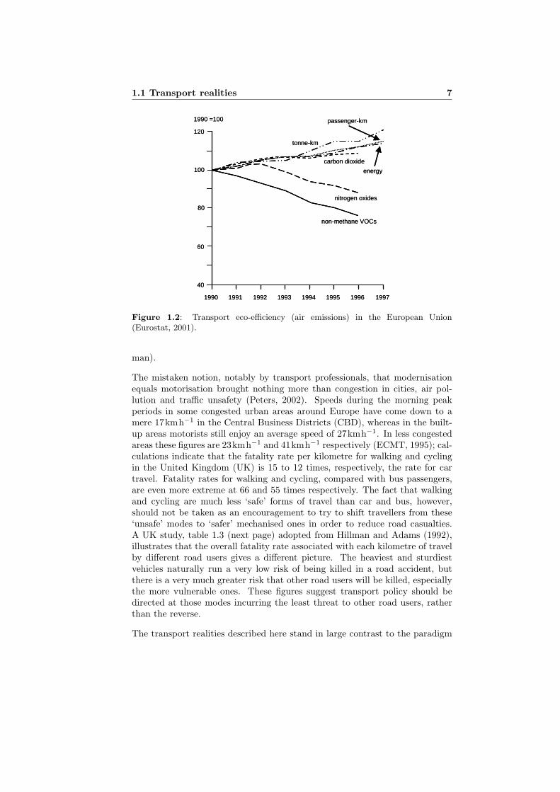
Between 1970 and 1997, passenger and freight transport in the EU increasedby an annual average of 2.8 and 2.6% respectively, while the growth in GrossDomestic Product (GDP) over the same period was 2.5%. For road and air-passenger travel particularly, the boost in demand can be attributed to higherincomes, a fall in transport prices in real terms and changes in travel patterns,because of urban sprawl, decreasing household sizes, and changing work pat-terns and lifestyles. In turn, the demand and intensity of freight transport isclosely linked to changes in the volume and structure of the economy and toinfrastructure supply. Energy and carbon dioxide efficiency (i.e. energy use perpassenger and per freight transport unit) has shown little or no improvementsince the early 1970s (see figure 1.2)). The increasing use of heavier and morepowerful vehicles, together with decreasing occupancy rates and load factors,has outweighed increases in vehicle energy efficiency due to technological ad-vances. As a result, growing transport volumes led to about a 14% increase inenergy consumption and a 12% increase in carbon dioxide emissions between1990 and 1997; figures that are still pertinent today. On the positive side, emis-sions of non-methane volatile organic compounds (VOC) and nitrogen oxideshave been falling since 1990 (also figure 1.2), mainly due to the introductionof catalytic converters in vehicle exhausts. However, the decrease has beenslower than expected as increasing transport demand has partly offset engineimprovements. Traffic noise is another key urban problem. It is estimatedthat over 30% of people in the EU are exposed to high road-traffic noise levels,about 10% of people to high rail noise levels, and possibly a similar proportionto aircraft noise (Eurostat, 2001). In addition, transport infrastructure takesland and may constitute a barrier against the movement of species (including
1.1 Transport realities 7
120
100
80
60
40
1990 1991 1993 19941992 1995 1996 1997
non-methane VOCs
nitrogen oxides
carbon dioxide
energy
passenger-km
tonne-km
1990 =100
120
100
80
60
40
1990 1991 1993 19941992 1995 1996 1997
non-methane VOCs
nitrogen oxides
carbon dioxide
energy
passenger-km
tonne-km
1990 =100
Figure 1.2: Transport eco-efficiency (air emissions) in the European Union(Eurostat, 2001).
man).
The mistaken notion, notably by transport professionals, that modernisationequals motorisation brought nothing more than congestion in cities, air pol-lution and traffic unsafety (Peters, 2002). Speeds during the morning peakperiods in some congested urban areas around Europe have come down to amere 17kmh−1 in the Central Business Districts (CBD), whereas in the built-up areas motorists still enjoy an average speed of 27kmh−1. In less congestedareas these figures are 23kmh−1 and 41kmh−1 respectively (ECMT, 1995); cal-culations indicate that the fatality rate per kilometre for walking and cyclingin the United Kingdom (UK) is 15 to 12 times, respectively, the rate for cartravel. Fatality rates for walking and cycling, compared with bus passengers,are even more extreme at 66 and 55 times respectively. The fact that walkingand cycling are much less ‘safe’ forms of travel than car and bus, however,should not be taken as an encouragement to try to shift travellers from these‘unsafe’ modes to ‘safer’ mechanised ones in order to reduce road casualties.A UK study, table 1.3 (next page) adopted from Hillman and Adams (1992),illustrates that the overall fatality rate associated with each kilometre of travelby different road users gives a different picture. The heaviest and sturdiestvehicles naturally run a very low risk of being killed in a road accident, butthere is a very much greater risk that other road users will be killed, especiallythe more vulnerable ones. These figures suggest transport policy should bedirected at those modes incurring the least threat to other road users, ratherthan the reverse.
The transport realities described here stand in large contrast to the paradigm

8 Introduction
Table 1.3: Fatality rates in the UK per 1.0 × 10⁸ vehkm to (Hillman and Adams,1992):
Mode Users Pedestrians Other All Other asthemselves users users a % of all
Bicycle 4.9 0.1 0.1 5.1 4Motorcycle 10.3 1.7 0.6 12.6 18Car 0.7 0.4 0.4 1.5 53Light freight 0.4 0.4 0.6 1.4 71Bus 0.4 1.8 1.7 3.9 90Heavy lorry 0.2 0.5 1.9 2.6 93
of a sustainable and developed transport system in which people have safe,quick and comfortable access to the activities they wish to perform while livingin harmony with their natural environment on the short and long run. Evenwhile some countries, notably the US administration, refuse, in contrast tomany other countries, to ratify the Kyoto protocol - that aims at significantlyreducing emission of Greenhouse gasses -, the Chinese government is banningout bicycles in their city centres - to make room for cars -, Mexico City, Beijing,Cairo, Jakarta, Los Angeles, Sao Paulo and Moscow (as seen in table 1.2)are competing to become number one polluted and congested megacities inthe world, it is believed that sustainable urban transport development shouldbe possible if a paradigm shift in thinking and acting is established, beforesustainable transport development becomes a paranoia instead.
This thesis aims to demonstrate the implications of a transport planning pa-radigm shift and to develop a corresponding analytical framework involvingchange from a given state of the transport system to a system compatible withsustainable development. The design concept and its feasibility will also bediscussed. The approach involved, combines elements from traditional reactivetransport planning and precautionary elements of environmentalism to reachwhat Deike Peters calls a sustainable mobility consensus (Peters, 2002).
Next paragraph2 discusses some basics on transport planning and transportmodelling theory, necessary to understand the alternative modelling conceptthat will be introduced in paragraph 1.3.
1.2 Transport planning
Transport policies have changed over time, in response to for example incre-asing vehicle performance and ownership levels, increasing congestion as wellas increasing awareness of environmental issues. Likewise, transport planningstrategies and objectives have changed from fully satisfying demand for trans-port to a more objective oriented, but trial-and-error based, transport plan-ning. Furthermore, as knowledge on travel behaviour of people in urban areashas improved, decision-makers, supported by transport modellers, were able
2Readers familiar with these theories may skip this paragraph up to section 1.2.3.

1.2 Transport planning 9
Transport
system
Activity
system
Flows
3
2
1
Figure 1.3: Basic relations of transport systems analysis (Manheim, 1979).
to change policy directions into management of road space. The basic issuesinvolved in transport system analysis and transport planning are discussed inthis paragraph.
1.2.1 Supply and demand
The transport system is closely linked to the social-economic system in an area.Back in the 1970s, Marvin Manheim posed the basic relations of transportsystem analysis; transport systems may shape societal and economic processesin the area. In return will these societal and economic processes indirectly affectthe shape of the transport system (Manheim, 1979). In a systems approachthree basic variables can be distinguished:
1. The transport system;
2. The activity system;
3. Traffic and transport flows.
Three basic relations between these variables are depicted in figure 1.3. First,the traffic and transport flows derive from the equilibration of transport systemsupply and the activity patterns that generate a travel demand. This is typi-cally a short to medium term relationship. Second, the traffic and transportflows might on the longer-term change activity patterns (shifts in modal choice,trip frequency choice etceteras) and eventually land-use patterns. Third, trafficand transport flows might necessitate changes in the transport system itself,through actions of traffic managers and transport planners. Urban transportplanning is concerned with this interaction, which is the equilibration of tra-vel demand, i.e. derived demand from the activity system, and infrastructuresupply, i.e. the characteristics of the transport system. It intends to steer theprocess of allocation of traffic generators and the provision of transport facili-

10 Introduction
Evaluation &
recommendations
Analysis, modelling
& forecasting
Diagnosis & issue
identification
Data collection &
system monitoring
Programming &
implementation
information about the current system
state; trends etc.
information about current/future
problems, policies etc.
information about the systems
performance, travel demand, impact
of alternative policies and future
states; understanding system
behaviour
information about benefit/cost
tradeoffs and cost/effectiveness of
alternative plans
information about priorities, staging,
implementation paths
Figure 1.4: The transport planning process (Meyer and Miller, 2001).
ties over space and time (Tolley and Turton, 1995).
Urban transport planning therefore tries to control the equilibrium flow inManheim’s systems approach. The urban transport planning process is de-picted in figure 1.4. Through the collection and monitoring of basic currentand expected future traffic and transport related data as well as the analysisof these data, the transport problems at hand are derived in relation to (fu-ture) political, social and economic developments. In addition, quantitativetechniques are applied to model, analyse and forecast alternative plans, and(future) scenarios. Several plans may then be evaluated on the basis of severalindicators (cost-benefit analysis, environmental impact assessment etceteras).Consequently, one or a combination of plans might be implemented. Manheim’ssystems approach is typically applied in the analysis, modelling and forecasting

1.2 Transport planning 11
phase of this planning process. This is accordingly called the urban transportplanning modelling system, or analytical transport planning model (TPM). Aswill become clear, this thesis focusses on the definition and operationalisationof such modelling techniques for the planning of sustainable urban transportsystems.
The equilibration of infrastructure supply and travel demand is often depictedas a travel market equilibrium (as seen in figure 1.3). Both supply and demandare treated as functions of costs, in transport terms generalised costs, i.e. a(non)linear combination of weighted disutilities like travel cost (out-of-pocketcost and variable cost) and travel time converted to monetary units using thevalue-of-time concept, applying parameters α and β. For example, the genera-lised cost expressed as a linear weighted combination of travel time and travelcost reads:
c = α · travel time + β · travel cost. (1.1)
The notion that the demand for travel, T , is a function of cost, c, presents nodifficulties. However, if the predicted travel demand were actually realised, thegeneralised cost might not stay constant. This is where the infrastructure supplymodel comes in. The classical approach defines the supply curve as giving thequantity T , which is produced, given a market price c. However, while certainaspects of the supply function do, of course, relate to the cost of providingservices, the focus of supply relationships in transport has very often been onthe non-monetary items, and on time in particular. In addition, the generalisedcost is often more straightforward seen as the inverse relationship, whereby cis the unit (generalised) cost associated with meeting a demand T . The supplymodel thus reflects the response of the transport system to a given level ofdemand; that is the deterioration in speeds as traffic volumes rise, or increasedparking problems as demand approaches capacity etceteras (Bates, 2001).
This equilibrium model is graphically depicted in figure 1.5 (next page). Con-sidering both the demand curve and supply curve 1, the equilibrium point withactual travel, or revealed demand, can be found where both curves cross. Thismodel can for example be used to see the effect of road expansion. Supplycurve 2 indicates the changed situation as new capacity is added. At low de-mand volumes generalised costs c1 do hardly change (non-congested area ofthe curve). However, at higher demands the generalised costs c2 tend to riseslower than before due to the higher capacity. Hence, some extra demand isinduced or generated, due to improved travel conditions. The latent demand isthe demand that has not (yet) been revealed or become manifest, but could berevealed due to other transport system changes. As travel demand is a deriveddemand from activities, there will be a limit to the amount of latent demandavailable (a market saturation).

12 Introduction
Generalized
cost (c)
Flow (T)
c2
supply 2
demand
supply 1
Revealed demand Latent demandInduced demand
c1
Figure 1.5: Demand-supply equilibria.
1.2.2 Transport modelling
The current approach in analytical transport planning or transport modelling,evolved from the 1960s, when the Chicago and Detroit transport studies wereperformed. The early approach is often characterised as a reactive, predict-provide approach in which vehicle and passenger volumes in the main travelcorridors were estimated and increases in road and public transport capaci-ties were proposed to accommodate those expected increases for the long-run.During that period the models were also typically single-mode, or unimodal.Since that period transport models have evolved3 into multimode, or multi-modal models (from begin 1970s), with a sound theoretical basis, notably theeconomic theory. Due to increased computing possibilities the transport modelshave become more disaggregated in detail level and have been applied at largerscales. Data collection techniques and estimation techniques have also impro-ved considerably. Major applications of transport models nowadays are withenvironmental impact assessments and road pricing measures. The traditional
3Nevertheless, the development of transport planning techniques has been evolutionaryrather than revolutionary (Bates, 2001).

1.2 Transport planning 13
Travel demand
predictions
Transport system, land-use and
socio/economic characteristics
Community (sustainability)
objectives
Transport service
and other policies
Design of transport system using
TPM
Prediction of travel and traffic
and other impactstrial-and-error feedback
Measures
Figure 1.6: Traditional transport modelling process (predict-provide).
transport modelling process is graphically depicted in figure 1.6. Future yearprojections of travel demand that are based on predicted transport system andtraffic characteristics, social-economic development as well as land-use plan-ning, together with some traffic and travel related measures, which are derivedfrom some transport policy objective (possibly based on explicit communityobjectives), form the basis for the design of the transport system using a trans-port planning model. At best there is a predict-provide feedback (throughtrial-and-error) from the predicted impact of transport and traffic figures backto the design of the transport system, in order to try to relief some of the trafficor other (negative) impact.
The so called Transport Planning Model (TPM) or traditional transport mo-del formed ever since the central part of the transport planning process (seefigure 1.4). In transport modelling, transport systems are depicted as networksG(N ,L), involving nodes n ∈ N (node-set N representing cities, zones, possi-bly also intersections etceteras), which are joint together by capacity restrainedlinks l ∈ L (link-set L representing roads, railways, etceteras). Each zone isrepresented with a zonal centroid from the centroid-set: Z = (I,J ) ⊂ N ,which consists of origins i ∈ I, and destinations j ∈ J . In every centroid alltrip origins and destinations are located, which generate the traffic flows alongthe links between the zones in the network. In addition, physical, demographicand social-economic variables useful to define the system of activities are alsoindicated in these centroids. Furthermore, a mode-set for vehicles m ∈ M aswell as origin-destination specific route-sets for routes r ∈ Rij are defined. Inaddition, R ⊃ Rij is the set of all routes, K the set with population segments kand P the set with pollutants p.

14 Introduction
Conventionally the traditional transport model, also four-step model, is dividedinto four sequentially linked sub models:
Trip generation, which is the number of trips associated with a zone at thenode end and consists of trips produced and trips attracted to that zone;
Trip distribution, which is the allocation of trips between each pair of zonesin the study area, thus producing an origin - destination (OD) trip table;
Modal split, which determines the number of trips by each mode of transportbetween each pair of zones;
Trip assignment, which allocates all trips by origin and destination zone tothe actual links that comprise the road network. Separate allocationsnormally take place for each mode. Trips are usually converted to vehicletrips using an average vehicle occupancy rate. Hence, this sub model isbetter named ‘traffic assignment’.
The first three sub models are concerned with the calculation of travel demand(in person trips) and the fourth sub model with the interaction with the trans-port system (to reveal vehicle trips). Bates (2001) gives a thorough descriptionon the first three sub models, which forms the basis for the model summarypresented here. The modelling of travel demand implies a procedure for pre-dicting what travel decisions people would wish to make, given the generalisedcost of all alternatives available to them. The decisions include choice of route(traffic assignment), mode (modal split), destination (trip distribution), andfrequency (trip generation). Often, the choice of time of travel is also added4.These choices can be linked together using choice hierarchies, implementingdiscrete-choice theory (for an extensive discussion on this topic the reader isreferred to amongst others Ben-Akiva and Lerman (1985)). Lower level choicesare made conditional on higher choices in a theoretically consistent way. Apossible, idealistic, structure is shown in figure 1.7. That is, most transportmodels around have a sequential structure, not having this possibility of feed-back. If this feedback is allowed, Manheim’s demand-supply equilibrium couldbe obtained.
The first sub model, the trip generation model, or trip frequency model can besubdivided into a trip production and trip attraction model. In general, thefirst one can be estimated quite accurately, using the general trip productionmodel:
Ti|k = f(x1i|k, x2i|k, · · · , xni|k; [c∗i|k]) = f(~xi|k; [c∗i|k]), (1.2)
where k is a population segmentation (usually trip purpose and social-economicbackground specific), i is the origin zone in the study-area, while the vector:~xi|k = x1i|k, x2i|k, · · · , xni|k, represents n social-economic characteristics for po-
4The time-of-day sub model is not considered in this thesis.

1.2 Transport planning 15
Destination choice
Ti***
Tij**
Tijm*
Tijmr
pj|i
pm|ij
pr|ijm
Trip frequency
choice
Mode choice
Route choice
Cijm*
Cijmr
Cij**
Ci***
Supply model
Figure 1.7: The traditional transport model, based on Bates (2001).
pulation segmentation k in zone i, whereas c∗i|k is the generalised cost, or com-posite cost of travelling from the origin zone i. Bates (2001) deliberately putsthese costs of travelling between brackets since it is hardly used in practice; tripproduction is usually treated as being dependent on exogenous variables to themodel only. This is done, even though it is very conceivable that the level of tripmaking is influenced by the transport system, hence introducing the concept ofaccessibility. The trip production equation is used to obtain the total numberof trip-ends in the zones of study. Most trip production models are householdor person-based, implying that a zonal aggregation has to be performed, using

16 Introduction
information on the total number of households per segmentation k in zone i,Hi|k, that is:
Ti = a0i +
∑
k
Hi|kf(~xi|k; [c∗i|k]), (1.3)
with a0i an intercept usually resulting from the model estimation, e.g. applying
techniques of multiple linear regression (see paragraph B.1).
Trip attraction models for Tj can have a similar structure as in equation (1.2),where the explaining variables for the different attractions in zone j are relatedto the type of land-uses attracting produced trips. In general, it appears rathercomplicated to find these figures. Ideally the trip attraction rates, like the tripproduction rates, are also dependent on the generalised cost between the zonesof production and attraction.
Since trip productions can be more accurately determined, trip attractions areusually balanced (in total made equal) to the total number of trip productions.Therefore, the trip attraction model merely serves as a distributor of tripsover the attractors. To balance the total number of trip productions and tripattractions a balancing factor f is applied to all trip attractions T ′j to obtainthe balanced Tj , which is:
f =T∑
j∈J T ′j, (1.4)
with the total number of trips being: T =∑
i∈I Ti.
In the second sub model, i.e. the trip distribution model, an OD - table, matrixTij , is constructed, relating the number of trips in the matrix cell (i, j) to:
1. the characteristics of the origin/production zone i;
2. the characteristics of the destination/attraction zone j;
3. the characteristics of the generalised cost of travel, between zones i and j.
This relation, named the gravity model after its apparent analogy with theNewtonian law of gravitation, has the general form:
Tij = µQiXjf(cij), (1.5)
where Qi is the production potential of zone i, Xj the attraction potentialfor zone j, µ the ‘gravity’ constant5 and f(cij) is a distribution function6, in
5Parameter µ is interpreted here as a measure of average trip intensity in an area, beingthe number of travellers P divided by the number of and variability in trip alternatives k,i.e.: µ = P
k(Bovy and Van der Zijpp, 1999).
6Also called deterrence function, or impedance function.

1.2 Transport planning 17
its early form depicted as f(dij), hence only considering the travel distancebetween zones i and j indicated as dij :
f(dij) =1
d2ij
, (1.6)
but nowadays often used in an exponential form with parameter λ, relatingthe distribution to the generalised or composite costs of travel between zo-nes i and j, cij :
f(cij) = exp(−λcij). (1.7)
The exact calculation of Tij usually assumes that trip productions and/or tripattractions from the trip generation sub model are known. In the productionconstrained trip distribution model, the number of trip productions Ti areimposed as a set of constraints:
∑j Tij = Ti, on the general trip distribution
model, after some calculations giving:
Tij = TiXjf(cij)∑
j′∈J Xj′f(cij′). (1.8)
Hence, the production constrained trip distribution model is a proportionalmodel that splits the known trip production numbers in proportion to theattraction potential Xj . Similarly, an attraction constrained trip distributionmodel can be constructed.
If both the number of trip productions and trip attractions are known thecalculation of Tij is usually performed as an iterative process known as bi-proportional fitting, or the Furness method, where two sets of constraintsare given, namely the numbers of arrivals:
∑i Tij = Tj , and departures:∑
j Tij = Ti, as well as two balancing parameters ai and bj , changing equa-tion (1.5) in:
Tij = aiTibjTjf(cij). (1.9)
Obviously, the matrix-total is:∑
i
∑j Tij = T .
In figure 1.7 this destination-choice model is depicted as a conditional proba-bility:
pj|i:k = f(c∗ij|k, cij|k : ~xi|k, ~zj), (1.10)
where, as before, k is a segmentation of the population, i and j again theorigin and destination zone, pj|i:k the proportion of all travellers of type k in

18 Introduction
zone i, who travel to zone j, c∗ij|k the composite cost of travel between zones i
and j, and cij|k the associate cost of travel to all zones, with j the set ofdestination zones J , and: ~xi|k = x1i|k, x2i|k, · · · , xni|k, the vector of n social-economic characteristics for segmentation k, while: ~zj = z1j , z2j , · · · , zn′j , isa vector of n′ zonal characteristics. The reader is referred to Ortuzar andWillumsen (2001) for a complete derivation of the gravity model.
Similarly, the third sub model, i.e. the mode choice model, can be formulatedas a conditional probability:
pm|ij:k = f(c∗ijm|k, cijm|k), (1.11)
where, as before, k is a segmentation of the population, i and j again theorigin and destination zone, m the mode, pm|ij:k the proportion of all travellersfrom population segmentation k moving between zone i and zone j who usemode m, c∗ijm|k the composite cost of travel between zones i and j by mode m,and cijm|k the associate cost of travel by all modes, with m the set ofmodes M being considered. The main sources of variation in the mode choicemodels, used in practice, according to Bates (2001) are:
1. the number and type of modes actually distinguished;
2. the detail of the generalised cost functions c∗ijm|k.
Mode choice models initially were bi-modal, requiring a sigmoidal curve whe-reby the probability of choosing the mode vanishes when its costs vary greatlyin excess of the costs of the other mode, but which allows reasonable sensiti-vity when the costs are comparable. For multimodal models, commonly usednowadays, the discrete-choice or multinomial logit (MNL) formulation of equa-tion (1.11) is used:
pm|ij:k =exp(−λ1|kf(c∗ijm|k))∑
m′∈M exp(−λ1|kf(c∗ijm′|k)), (1.12)
with λ1|k the ‘spread’ parameter or scale parameter reflecting the degree ofsubstitutability between the modes m, in other words the sensitivity of choiceof mode to changes in generalised cost, or utility c∗ijm|k. Often, λ1|k is chosen tobe unity, as in the Maximum Likelihood Estimation (see appendix B.2) of themodel, it gets integrated in the parameters for the utility function f(c∗ijm|k),denoted as utility or disutility uijm|k in short (see below). The effect of va-riations in the value of λ1|k, for the binomial case, is depicted in figure 1.8.At lower values of λ1|k changes in decision choice, in this case choosing foralternative 1 with disutility, or travel impedance u1, in relation to alternative 2with disutility u2, are smoother.
Utility is considered to be the value that individuals derive from choosing a cer-tain alternative, in other words utility is related to the (relative) attractiveness

1.2 Transport planning 19
−10 −5 0 5 10
0.1
0.2
0.3
0.4
0.5
0.6
0.7
0.8
0.9
1
p(u 1)
(u1−u
2)
λ1 = 0.2
λ1 = 0.35
λ1 = 0.9
λ1 = 2
Figure 1.8: Diversion curves for decision choice behaviour.
of alternatives. The net-utility for mode alternative m, for example, experien-ced by individual or population segmentation k consists then of a measurable,or systematic part vm|k and a random part εm|k, representing particular taste-values, but also observational errors made in the modelling:
um|k = vm|k + εm|k. (1.13)
The measurable part vm|k may be a function of several attributes, like thetravel characteristics, travel time and travel cost per mode, with parameters asin equation 1.1. Similar to neoclassical economic theory, the alternative withthe highest utility is supposed to be chosen. Therefore, the probability thatalternative m is chosen by decision-maker type k within choice-set M is:
pm|k = p
[um|k = arg max
m′∈Mum′|k
]. (1.14)
The mode-specific travel demand Tijm can now be calculated using the discrete-choice model (1.12):
Tijm = θmTij pm|ij:k, (1.15)
where θm is the vehicle m occupancy factor.
The travel demand Tijm is in the fourth sub model confronted with the supplymodel representing the transport system itself. Hence, in the traffic assignment
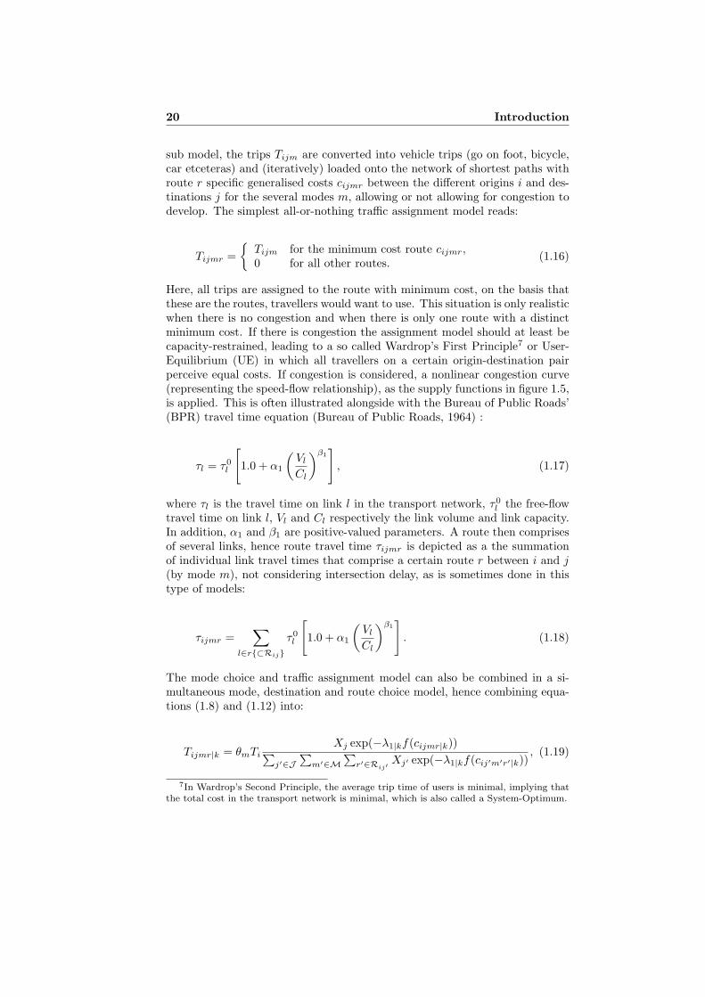
20 Introduction
sub model, the trips Tijm are converted into vehicle trips (go on foot, bicycle,car etceteras) and (iteratively) loaded onto the network of shortest paths withroute r specific generalised costs cijmr between the different origins i and des-tinations j for the several modes m, allowing or not allowing for congestion todevelop. The simplest all-or-nothing traffic assignment model reads:
Tijmr =
Tijm for the minimum cost route cijmr,0 for all other routes. (1.16)
Here, all trips are assigned to the route with minimum cost, on the basis thatthese are the routes, travellers would want to use. This situation is only realisticwhen there is no congestion and when there is only one route with a distinctminimum cost. If there is congestion the assignment model should at least becapacity-restrained, leading to a so called Wardrop’s First Principle7 or User-Equilibrium (UE) in which all travellers on a certain origin-destination pairperceive equal costs. If congestion is considered, a nonlinear congestion curve(representing the speed-flow relationship), as the supply functions in figure 1.5,is applied. This is often illustrated alongside with the Bureau of Public Roads’(BPR) travel time equation (Bureau of Public Roads, 1964) :
τl = τ0l
[1.0 + α1
(Vl
Cl
)β1]
, (1.17)
where τl is the travel time on link l in the transport network, τ0l the free-flow
travel time on link l, Vl and Cl respectively the link volume and link capacity.In addition, α1 and β1 are positive-valued parameters. A route then comprisesof several links, hence route travel time τijmr is depicted as a the summationof individual link travel times that comprise a certain route r between i and j(by mode m), not considering intersection delay, as is sometimes done in thistype of models:
τijmr =∑
l∈r⊂Rijτ0l
[1.0 + α1
(Vl
Cl
)β1]
. (1.18)
The mode choice and traffic assignment model can also be combined in a si-multaneous mode, destination and route choice model, hence combining equa-tions (1.8) and (1.12) into:
Tijmr|k = θmTi
Xj exp(−λ1|kf(cijmr|k))∑j′∈J
∑m′∈M
∑r′∈Rij′
Xj′ exp(−λ1|kf(cij′m′r′|k)), (1.19)
7In Wardrop’s Second Principle, the average trip time of users is minimal, implying thatthe total cost in the transport network is minimal, which is also called a System-Optimum.

1.2 Transport planning 21
where the total utility f(cijmr|k) of a destination-mode-route choice combinati-on for a given origin, is expressed as a function of individual measurable choice-utility components v and accompanying random elements ε (compare equati-on (1.13)), noting that utility directly consists of time and cost elements c:
f(cijmr|k) ≡ uijmr|k = vij|k +vijm|k +vijmr|k +εij|k +εijm|k +εijmr|k. (1.20)
This formulation only holds when the individual choice-utility components areassumed to be non-correlated or independent, and parameter λ1|k is unique forthe combined choice; see Oppenheim (1995) for a discussion on such formu-lation. A multinomial logit model then results, in which the argument is theconditional utility (based on travel time τijmr|k and travel costs κijmr|k) fora given simultaneous origin i, destination j, mode m and route r alternative,alike equation (1.1), i.e.:
uijmr|k = α τijmr|k + β κijmr|k. (1.21)
From this simultaneous mode, destination, route choice model or the standardtraffic assignment sub model, the vehicle link flows qv
lm and link travel times τl,hence link speeds sl, can be obtained through link-route incidence.
Several forms of ex-post traffic impact analysis can now be performed usingthe information revealed in the different sub models, ranging from selectedlink analysis, for example to reveal congestion levels, to different types of en-vironmental impact studies by applying environmental models, thus revealingdata on energy consumption, traffic emissions and noise pollution. An exampleof determining total traffic emissions Ep for transport pollutant p ∈ P in atransport network is adapted from Zietsman (2000), i.e.:
Ep =∑
l∈L
∑
m∈Mqvlm R∗slmp dl, (1.22)
with R∗slmp the composite emission rate for pollutant type p and mode type m,at the average link speed sl; dl is the length of link l. Similarly, the noisepollution can be calculated per link in the transport network. The equivalentcontinuous sound level Leq
l measured in decibel [dB] can be obtained using thefollowing equation, also obtained from Zietsman (2000):
Leql = 10 log10
[φ
15
∑m
(qvlm)B
(15DE
)1+υ]
, (1.23)
where φ is the equivalent subtending angle, υ a land dampening factor, DE anequivalent lane distance and B a function of total traffic volume, mode specifictraffic volumes and associated mode specific mean speed, or overall mean speed.

22 Introduction
More specific exogenous data on the local surrounding area is sometimes usedto reveal more detailed noise and traffic pollutant emissions. An example canbe found in the Promil model that is used in The Netherlands in combinationwith transport models and Geographical Information System (GIS) data onthe area (Goudappel Coffeng, 2003).
In a similar fashion other effects and impacts can be obtained, like fuel con-sumption, total number of kilometres travelled in the transport network8, totalnumber of passenger trips made and (more difficult) traffic unsafety. However,it should be realised that all these impact models don’t feature any feedbackto the sub models of the transport model.
1.2.3 Transport modelling alternatives
Despite the fact that limitations of the conventional transport model, in parti-cular the four-step transport model described above, are well known by trans-port professionals it has been used worldwide ever since the 1960s. Some ofthe limitations often posed are summarised from Banister (2002):
• The positivistic approach that is data driven and makes no attempt atunderstanding the real mechanisms of people’s travel behaviour. Travelis a derived demand and can be quantified using empirical relationships;
• The sequential decision-making process, whereas there is clear evidencethat (travel) decisions are made simultaneously. The feedback loops thatmay describe a more realistic decision-making process, as in figure 1.7,are seldom used;
• The aggregated character of the models, e.g. zonal aggregation, ignorepatterns and uncertainty in behaviour;
• The interactions between land-use and transport through land-use varia-bles, as well as social-economic variables like employment and populationare conventionally modelled as exogenous variables;
• The structure of the four-step model makes it difficult to include uncon-ventional or radical policy alternatives;
• Most transport models are static and are calibrated on one set of cross-sectional data only. Hence, coefficients are assumed to be stable overtime;
• Not all significant variables are specified in the model, or strong assump-tions have been made about them;
• Variability of travel over time is ignored. The time unit of analysis isoften the morning peak period.
8Often the expression Vehicle Mileage Travelled (VMT) is used.

1.2 Transport planning 23
These limitations, causing a lot of criticism over the past 20 years, are, unfortu-nately, still relevant today and reflect the in-built resistance to or impossibilityof radical change by transport planners. To respond to some of the shortco-mings of the traditional transport models in the 1970’s and 1980’s researchershave been trying to improve the existing approach, most importantly includingthe discrete-choice models, which lead to:
• The development of land-use transport models, in which the variableland-use is endogenised. The complexity of input data and the choicemodels in this case, however, is even more demanding than the traditionaltransport model;
• The development of disaggregate behavioural models that model the indi-vidual choice process on a micro level, being person-based or household-based, instead of the aggregate behavioural assumptions that were madein the earlier versions of the traditional transport model;
• The development of disaggregate utility models to better model the choicebehaviour of individuals confronted with several options (assuming fullinformation on the alternatives);
• The development of activity-based models that explicitly model travel asa derived demand from activities undertaken instead of the direct demandassumed in the traditional transport model.
In the 1990’s and 2000’s the basic framework for transport analysis remainedas it was in the 1960’s, though some other developments have taken place, i.e.:
• A shift in focus from the long-term strategic to more medium-term tac-tical/operational models, also called Integrated Transport Studies (ITS);
• A focus on evaluation methods as Cost Benefit Analysis (CBA) as wellas Environmental Impact Assessment (EIA), coupled with the traditionaltransport model;
• Stated preference (SP) and contingency valuation methods, to reveal pre-ferences for and the value of, not (yet) existing, choice alternatives, foruse in the discrete-choice model;
• Dynamic analysis to reveal more information on long-term elasticities inbehaviour of people;
• Large-scale land use and transport demand studies, based on large data-sets, mainly for analysing and monitoring system performance.
In this research it is by no means tried to resolve all mentioned limitationsand shortcomings to the traditional transport model, because it would be anunfeasible exercise as many researchers have been trying to do so, with variousresult. Instead, some major shortcomings that are considered to be indispu-tably related to the topic of this thesis, i.e. sustainable development of urbantransport systems, are dealt with. These are discussed in next paragraph.

24 Introduction
1.3 Strategic transport planning
In view of the transport realities described before, the theory of sustainabledevelopment and sustainable urban transport development - further developedin chapter 2 - and above mentioned critiques to conventional transport systemanalysis, a conceptual analytical framework and an accompanying dynamictransport model for sustainable urban transport development are proposed inthis thesis. There are three main reasons for doing this. First, a directly appli-cable analytical conceptual framework for sustainable urban transport devel-opment, focussing on possible application within (strategic) transport planningand modelling, is not yet existing. Second, the requirements derived from theconceptualisation of sustainable urban transport development are not yet in-ternalised in the traditional transport planning model, partly because the ana-lytical framework is not existing, partly because it is not a trivial exercise todo so. Third, conventional transport models can hardly produce useful recom-mendations to decision-makers if they are not founded on the understandingof the continuously changing behaviour of its users (the trip makers), the per-formance of the transport system itself as well as the complex and interactingobjectives by its decision-makers.
The internalisation of requirements for sustainable development in transportplanning models necessitates a couple of fundamental changes (in arbitrary or-der) to the existing modelling; First, the omission of feedback to higher-levelsub models, mainly because of its complexity should be tackled; in particular inrelation to the inelasticity of the trip frequency model to changes in transportsystem performance. Second, the static character of the transport model isdeemed unsuitable, because sustainable development is a dynamic process byitself, whereas the different processes of generating travel demand and chan-ging infrastructure supply require different time scales, hence urging the useof dynamic models, particularly because of the medium to long-term characterof the concept of sustainable development. Third, sustainability demands theinclusion of externalities like traffic pollution and their system limits, which isoften not the case in current modelling techniques. Fourth, because of the inhe-rent complexity of transport system analysis and its (dynamic) equilibrium, aspreviously indicated in figure 1.3, it is believed that transport measures takento reach a certain policy objective, as well as the policy objective itself, shouldalso be endogenised in the process, hence seeking transport system optimafor the considered policy objective instead of using a predict-provide (throughtrial-and-error) feature. Hence, the model is objective-led, featuring a provide-predict structure.
Even, though, particularly for use in medium to long term strategic planning,the basic building blocks in the traditional modelling by itself are believed tobe adequate, above mentioned fundamental problems should be resolved in or-der to make these models suitable for the task of deriving transport policiesaimed at sustainable urban transport development. Hence, this thesis presentsa dynamic modelling based on the traditional modelling framework that can

1.3 Strategic transport planning 25
Travel demand
predictions
Community
(sustainability) objectives
Transport service and
policy objective
Design of transport system using
dynamic TPM
Prediction of travel and traffic and other
impacts over time
Acceptable levels of
resource consumption
Policy control
paths
Transport system, land-use and
socio/economic characteristics
Figure 1.9: Alternative transport modelling process (provide-predict).
optimise transport systems on the basis of a certain transport policy objecti-ve, while restricted by sustainability requirements, over time. This can thenbe used for strategic transport planning, as it produces medium to long termdynamic travel and traffic figures as well as the policy control paths that opti-mise the chosen sustainable transport policy objective for the transport systemunder study. This implies that the traditional predict-provide transport mo-delling process - which can be typified as following a: ‘What if?’ strategy -from figure 1.6, changes into the provide-predict sustainable transport model-ling process - typified as following a: ‘How to?’ strategy - as is depicted infigure 1.9.
Strategic transport planning has its roots in long term planning of transportinfrastructure and is based on the assumption that decision-makers are res-ponsible for defining objectives and hence decide on a medium to long termtransport strategy including sets of transport measures. Strategic transportplanning, which is based on the same principles as ‘normal’ transport planning,is therefore typically broad and indicative, in the sense that further detailingof strategies (in time and over time) is required. Such an approach is followedhere also.
Hence, the type and detail of decisions that are considered here, can be typifiedas tactical to strategic. In particular, because this is in line with the mediumto long-term perspective that goes with sustainable development. This is welldescribed in Ortuzar and Willumsen (2001), who assume a trade-off betweenthe time horizon of the transport planning decision and the level of detail. At astrategic level, analysis and choices have major system-wide and long-term im-pacts, and usually involve resource allocation and network design. At a tacticallevel a somewhat more detailed perspective is chosen, involving questions like

26 Introduction
Detail
Time horizon of decisions
Tactical
Strategic
Operational
'Comprehensive'
Figure 1.10: Trade-offs in strategic, tactical and operational transport planning,adopted from Lee (1994).
making the best use of facilities and infrastructure. At the short-term a detai-led perspective can be adopted, i.e. an operational level of analysis that mayinclude detailed capacity analysis at the link level. This trade-off between per-spectives and time horizon of decision-making is depicted in figure 1.10, whichis adopted from Lee (1994). The level of decision-making focused on in thisthesis, can alternatively be considered as comprehensive, following Lee (1994),as it will show to cover both tactical as well as strategic levels of analysis.In addition, for final and detailed information on, for example, local impacts,the operational level of analysis can still be deployed in combination with thestrategic level outcomes, by, for example, adopting a hierarchical modellingapproach. The strategic level then functions as indicative and direction-givingfor the operational and tactical levels as well as provides a first partitioning ofalternatives.
Transport planning seen as an optimisation process gives transport professio-nals at a strategic or comprehensive decision level, ample possibilities of havingsets of policy and engineering measures defined on the basis of a commitment toa certain (sustainable) transport policy objective; yet still complying with thebehavioural mechanisms known from traditional transport models. Optimaltransport strategies may thus be identified.
The proposed modelling differs from the static frameworks on which it is built,

1.4 Problem statement and research questions 27
through its:
Dynamics Transition paths towards a sustainable and developed transportsystem are revealed;
Optimisation The nature of the problem of designing a sustainable transportplanning is that of a constrained optimisation problem. The effects of differenttransport policy objectives can be studied and compared;
Controls Engineering interventions, such as road construction, road main-tenance and public transport priority, as well as pricing measures, like vehicletaxes, parking taxes and bus fares, are the tools, or controls, to the decision-maker;
Constraints Resource constraints and physical constraints to the controls areapplied.
Next, a problem statement with accompanying research questions is given.
1.4 Problem statement and research questions
The previous sections gave a nutshell description on the (urban) transportproblems and issues that are considered pertinent when discussing (strategic)transport planning and sustainability. Urban transport problems and the requi-rements for sustainable development are increasingly complex. Current trans-port systems and transport planning models (used in developing and developed)countries are not necessarily compatible with the requirements of sustainabletransport development. Adequate transport systems can only be obtained withuse of a new transport planning paradigm and accompanying analytical frame-work.
A suitable analytical transport planning technique distinguishes itself from tra-ditional planning techniques if it is directly based on a conceptualisation ofsustainable development and when it is able to adequately cope with the ob-served drawbacks with current transport modelling (in particular related to thedefinition of sustainable development). That is, the current process determi-nes a static equilibrium solution, whereas sustainable transport developmentby definition is a dynamic phenomenon with several and different coevolvingstates of its individual systems and users. Moreover, the trip frequency modelis considered deficient in its inability to estimate generated or latent demandwhen transport system performance changes. In addition, sustainable trans-port development requires a balanced set of planning instruments that reckonswith positive as well as negative externalities that come with transport, whilecomplying with a certain transport policy objective, something which is notexplicitly considered in current transport modelling.
Definition and description of the implications of adopting a sustainable trans-

28 Introduction
port development paradigm as well as the development of an analytical frame-work and model for sustainable urban transport development are the topic ofthis thesis. A problem statement and research questions are given below.
The basic problem addressed in this thesis is:
Problem definition: What are the requirements for sustainable urban trans-port development and what are the implications of these requirements fortransport planning, in particular transport modelling?
Internalisation of the concept of sustainable development implies using thisconcept in the development of new transport systems and plans as well as themanagement of existing ones. The focus, however, is on the analysis, modellingand forecasting stage of the transport planning process depicted in figure 1.4.The implications of this internalisation on the total transport planning processare, of course, also identified.
The major aim of the research is therefore:
Research aim: To define and describe the requirements for sustainable ur-ban transport development as well as to develop an analytical transportplanning method and tool, in which these principles of sustainable devel-opment are internalised, and to demonstrate plausibility and feasibilityof the ideas and method.
Hence, the research aims at contributing to the achievement of an overall sustai-nable development in urban areas around the world. Sustainable development,however, goes much further than urban transport sustainability alone. And,also within transport there are many different areas that contribute to sustai-nability, amongst others freight, maritime transport as well as air transport.However, this thesis will only focus on passenger transport in urban areas. Ata geographical scale this research is not limited to cities in developing or devel-oped countries. Both type of cities will somehow be discussed, as the specificmanifestation of their urban transport problems may differ, but the underlyingtransport mechanisms are assumed to be the same.
On a more detailed scale, this study intends to answer the following threeresearch questions:
Research question 1: What are the implications of the notion and definitionof sustainable development for urban transport planning?
Research question 2: How should sustainable development be modelled andincorporated in urban transport planning practice?
Research question 3: What typical consequences can be expected and im-plications be drawn for urban transport planning in the long-term due tointernalisation of the concept of sustainable development?

1.5 Limitations of this research 29
The remainder of this thesis is confined with the answering of these researchquestions, which are successively addressed throughout the three parts of thisthesis.
1.5 Limitations of this research
The research described in this thesis is limited to the study of sustainabledevelopment in urban transport planning and modelling; in particular urbanpassenger transport, i.e. the movement of people in transport networks wheredestination, mode and route choice behaviour are prevalent. However, it istried to keep the introductory chapters 1, 2 and 3 general introductions insustainable development and transport.
Sustainable development is known to be a complex and integrated issue. Afull integration will probably never be accomplished. Putting too many requi-rements on the concept may even lead to failure of achieving anything appro-aching a sustainable system. Therefore, it is always tried to keep the readerinformed where, how and why part of the integration is not established.
The focus in this research is on quantitative aspects of transport planningat a strategic application level. Furthermore, the author’s reasoning comesprincipally from an engineering and mathematical economics point of view.
1.6 Scope and outline of this thesis
This thesis is divided into three main parts. The remainder of this part, part I,deals with the concept of sustainability and sustainable development. In chap-ter 2, a conceptual framework for sustainable development is given and linkedto transport. Some of the many concepts and definitions are given and discus-sed. A conceptualisation of sustainable transport is then given that is adoptedin the remainder of the research. In chapter 3, some more detail is given on thelinkage between travel, infrastructure and sustainable urban transport develop-ment. Part II deals with modelling sustainable urban transport development.First, in chapter 4, the intended use of optimisation as a tool for sustainabletransport policy design is discussed. Followed, in chapter 5, by a descriptionof the dynamic transport model, including some background on mathematicalsystems theory. Finally, part III deals with an analysis of the implications ofusing the concept and dynamic transport model for (strategic) transport plan-ning in chapter 6. The intended use of the model in real-life is also discussed.The several consequences that can be expected and implications that can bedrawn for urban transport planning in the long-term due to internalisation ofthe concept of sustainable development are given on the basis of these examplesin the concluding chapter 7. This thesis ends in chapter 8 with a short reflexivedialogue on transport sustainability with respect to developing countries.

30 Introduction
1 2 3
4 5
6 7 8
I
II
III
Concept
Modelling
Application
Figure 1.11: Structure of the thesis.
The structure of the thesis, including part and chapter numbers, is given infigure 1.11.

Chapter 2
Sustainable developmentand transport
2.1 The Limits to Growth
In 1972, also the year that the first United Nations Conference on the HumanEnvironment was held in Stockholm, Sweden, an influential book was publis-hed named The Limits to Growth by Meadows et al. (1972). It described theprospects for growth in the human population and the global economy for the20th century. This document created an uproar. The combination of the use ofa computer model, and the involvement of The Club of Rome and Massachu-setts Institute of Technology (MIT) pronouncing upon pending disaster had anirresistible dramatic appeal.
The three main conclusions in this book were (Meadows et al., 1972):
1. If the present growth trends in world population, industrialisation, pol-lution, food production, and resource depletion continue unchanged, thelimits to growth on this planet will be reached sometime within the next100 years. The most probable result will be a sudden and uncontrollabledecline in both population and industrial capacity;
2. It is possible to alter these growth trends and to establish a condition ofecological and economic stability that is sustainable far into the future.The state of global equilibrium could be designed so that the basic ma-terial needs of each person on earth are satisfied and each person has anequal opportunity to realise his or her individual human potential;
3. If the world’s people decide to strive for this second outcome rather thanthe first, the sooner they begin working to attain it, the greater will betheir chances of success.
In other words, physical limits to growth exist and, if and only if fully respected,an equitable distribution of well-being is regarded feasible.
31

32 Sustainable development and transport
In 1984, the World Commission on Environment and Development (WCED)was established with the task of formulating ‘a global agenda for change’, whichresulted in 1987 in the publication of the Our Common Future, or Brundt-land report by WCED (1987)1. This report investigated the capacity of theearth to support its population and the ways in which human activities wereaffecting the environment. The Brundtland Commission defined sustainabledevelopment as ‘development which meets the needs of the present withoutcompromising the ability of future generations to meet their own needs’.
The two key aspects in this definition and the accompanying Brundtland reportare:
1. the realisation of basic needs for all people, in particular those in need;
2. the limits to growth are technical, cultural and social.
These aspects contrast to the limits of growth of Meadows et al. (1972), whichare merely environmental and resource availability. Basically, the Brundtlandreport rejects the physical limits to growth and stresses the belief that equity,growth and environmental sustainability are simultaneously possible.
In 1992 there would be a sequel to the initial The Limits to Growth publicati-on, influenced by amongst others critique to the 1972 publication, the publicdebate on sustainable development that commenced since the appearance ofthe Brundtland report as well as the second United Nations Conference onEnvironment and Development (UNCED) in 1992 in Rio de Janeiro, Brazil,where another important document was launched, i.e. Agenda 21, in whichit is advocated that individual countries should prepare strategies and actionplans to implement sustainability2,3. In this sequel Beyond the Limits the sa-me authors, Meadows et al. (1992), alter some of the assumptions from 1972,reconfirm some of the conclusions of 1972 and show that some limits of growthhave been reached or even surpassed. Some options for sustainability have beennarrowed, others have opened up. The three main conclusions of 1972 are in1992 rewritten as (Meadows et al., 1992):
1. Human use of many essential resources and generation of many kinds ofpollutants have already surpassed rates that are physically sustainable.Without significant reductions in material and energy flows, there will bein the coming decades an uncontrolled decline in per capita food output,energy use and industrial production;
1Named Brundtland report after the chairwoman of the WCED, Gro Harlem Brundtland,who nowadays heads the World Health Organization (WHO).
2On a smaller geographical scale often Local Agenda 21 ’s are introduced to indicate stra-tegies and action plans for sustainability by regions, cities or small communities.
3Unlike the Meadow’s reports as well as the Brundtland report, Agenda 21 specificallymentions traffic and transport strategies as tools for achieving a sustainable society. See forexample Chapter 7: Promoting sustainable human settlement development, Programme area(e): Promoting sustainable energy and transport systems in human settlements, in UNCED(1992).

2.1 The Limits to Growth 33
2. This decline is not inevitable. To avoid it two changes are necessary. Thefirst is a comprehensive revision of policies and practices that perpetuategrowth in material consumption and in population. The second is arapid, drastic increase in the efficiency with which materials and energyare used;
3. A sustainable society is still technically and economically possible. Itcould be much more desirable than a society that tries to solve its pro-blems by constant expansion. The transition to a sustainable society re-quires a careful balance between long-term and short-term goals and anemphasis on sufficiency, equity and quality of life rather than on quantityand output. It requires more than productivity and more than technolo-gy; it also requires maturity, compassion and wisdom.
In other words, human activities are affecting the environment, hence technical,cultural and social limits are imposed, not just environmental resource limitsas was the case in the 1972 episode.
Again these conclusions were based on (by that time) extensive computer simu-lations of different global scenarios, applying system dynamics models. Becauseof the global character, transport was obviously not an explicit part of the mo-dels. Figure 2.1 (next page) shows three scenarios that have been calculatedin Meadows et al. (1972) as well as Meadows et al. (1992). Scenario (a) showsthe ‘standard’ run from The Limits to Growth, in which the computer modelWorld3 is run that models stocks as population, industrial capital, pollutionand cultivated land. Those stocks change through flows such as births anddeaths, investment, depreciation, pollution generation and pollution assimila-tion. The causal relationships between them are highly nonlinear. Populationand industry output grow until a combination of environmental and naturalresource constraints eliminates the capacity of the capital sector to sustain in-vestment. In scenario (b) a doubled stock of exploitable resources is assumed.Industrial outputs may grow a mere 20 years longer, but otherwise nothing isgained and the fall is all the steeper. The general behaviour of the model is,like in scenario (a), overshoot and collapse. The system is drawing resources oremitting pollutants at an unsustainable rate, but the stresses on the supportsystem are not yet strong enough to reduce the rates of withdrawal or emission.This overshoot comes from the delays in feedback - from the fact that decisi-on makers in the system do not get, or believe, or act upon information thatlimits have been exceeded until long after they have been exceeded (Meadowset al., 1992). In that case overshoot may even convert to collapse. Scenario (c)presupposes that sustainability policies, including those directed at populationgrowth, were implemented as early as 1975. It shows that society reaches itsdesired level of industrial output per person and is able to maintain it andsupport its improving technologies with no problems. Unfortunately, doing thesame now, doesn’t prevent heavy turbulence to occur. Hence, the title Beyondthe Limits ...

34 Sustainable development and transport
Food
1900 2100
State of the world
Resources
Industrial output
Population Pollution
1990 2000
Environmental pollution
1900 2100
Global scenario
Raw materials
Food supply
Industrial productionPopulation
20001990
2100
Environmental pollution
1900
Global scenario
Raw materials
Food supply
Industrial production
Population
20001990
Food
1900 2100
State of the world
Resources
Industrial output
Population Pollution
1990 2000
State of the world
Resources
Industrial output
Population Pollution
1990 2000
Environmental pollution
1900 2100
Global scenario
Raw materials
Food supply
Industrial productionPopulation
20001990
Environmental pollution
1900 2100
Global scenario
Raw materials
Food supply
Industrial productionPopulation
20001990
2100
Environmental pollution
1900
Global scenario
Raw materials
Food supply
Industrial production
Population
20001990 2100
Environmental pollution
1900
Global scenario
Raw materials
Food supply
Industrial production
Population
20001990
Environmental pollution
1900
Global scenario
Raw materials
Food supply
Industrial production
Population
20001990
(a)
(b)
(c)
Figure 2.1: (a) The standard run from The Limits to Growth. Population andindustry output grow until a combination of environmental and natural resourceconstraints eliminate the capacity of the capital sector to sustain investment; (b)Assuming a doubled stock of exploitable resources, industrial outputs may grow amere 20 years longer, but otherwise nothing is gained and the fall is all the steeper;(c) The sustainability scenario presupposes that strict sustainability policies includingon population, were introduced as early as 1975 (Meadows et al., 1992; Meadowset al., 1972).

2.2 Sustainability and sustainable development 35
Ten years after Rio de Janeiro, in 2002, progress on the ideas and targets setby the Brundtland Commission have been discussed in Johannesburg, SouthAfrica. Although this summit has been criticised for failing to set and renewconcrete targets, renewed commitment for action, in particular strengtheningthe role of the private sector, in achieving sustainability and sustainable devel-opment were obtained.
2.2 Sustainability and sustainable development
Sustainable development strives for an optimal balance between economic, so-cial and ecological objectives. Sustainability thinking reflects concerns aboutlong-term risks of current resource consumption, keeping in mind the goals ofintergenerational equity. This is posed clearly in the more detailed definitionon sustainable development, which is also defined by WCED (1987): ‘in essencesustainable development is not a fixed state of harmony, but rather a processof change in which the exploitation of resources, the direction of investments,the orientation of technological investment, and institutional change are all inharmony and enhance both current and future potential to meet human needsand aspirations’. The starting point is given by economic and social develop-ment that can satisfy human needs and aspirations, but also takes into accountthe natural resource base and social equity. Unlike both Meadows’ reports, theBrundtland report takes a more positive stand, in stating that the world’s re-sources are sufficient to meet long-term human needs. A distinction, however,should be maintained between growth (increased quantity) and development(increased quality) (Daly, 1991). Sufficiency and efficiency are important key-words for development4.
There is some confusion about the meaning of sustainable development. Thishas to do with the various interpretations of the terms sustainability and devel-opment. The underlying philosophy of sustainable development indicates thatit involves two main aspects - sustainability and development. In addition, thebasic idea is to harmonise the two aspects in societal activities. However, thefocus of most people and organisations is only on sustainability and is inter-preted exclusively in terms of keeping the environment in a notionally ‘good’condition. Sustainability is then a set of restrictions that must be met by so-ciety. If these restrictions, which depend on the physical boundaries of natureand maximum capacity of the system for the various resources consumed, areviolated, overshoot and collapse may result as seen in paragraph 2.1. Parallelto this, development is often seen as the process of a continued economic andsocial change, developing, but also developed countries, undergo. The standardof well-being or social welfare is improved, ideally maximised. Considering bothaspects simultaneously, a framework of sustainable development is dynamic andrelates the factors that define when a system is sustainable to the maximisation
4Some reports to The Club of Rome specifically deal with this increase in resource produc-tivity, notably halving resource use in Van Dieren (1995) and more recent, doubling wealth,while halving resource use in Factor Four by Von Weizsacker et al. (1998).

36 Sustainable development and transport
Maximize human potential
Sustainable
development
Maintain resilience of the
ecological, social and
economic systems
Non-
declining
levels of
welfare, or
utility
Maintain
critical
thresholds
of resource
use
Figure 2.2: A schematic representation of sustainable development, adapted fromESCAP-AITD (2001).
of social welfare, or more general human potential. This framework, read asa dynamic process, rather than as a static objective of optimisation, followingESCAP-AITD (2001), is shown in figure 2.2. Non-declining levels of welfare,or more general non-decreasing utility levels, guarantee that human potentialremains constant or is improved over time, while keeping the critical thresholdsor capacities of the different resources consumed by the system. The abilityof the system to absorb internal and external disturbances to its environmentand restore the balance (or equilibrium) is called the resilience of the system.
This resilience relates to another important discussion in defining sustainabi-lity, i.e. that of strong versus weak sustainability. Strong sustainability refersto non-decreasing patterns of environmental and resource stocks over time.Weak sustainability allows them to decrease temporarily so long as they re-turn to their initial levels. In this case single stocks may decrease and evenbe exhausted, so long as the aggregate condition is being satisfied at all ti-mes. Non-renewable resources such as stocks of fossil fuels and ores provide aspecial problem in this discussion. While for renewable resources maintenan-ce of stocks is a legitimate objective, for non-renewables the basic questionis how much resources should be left available to future generations (Van denBergh, 1991). Herman Daly’s interpretation of a sustainable society in his bookSteady-State Economics (Daly, 1991) is an example of a strong approach, inwhich environment is interpreted as a combination of natural and man-madeconditions. According to him a sustainable society is one that satisfies threebasic conditions, i.e.:
1. Its rates of use of renewable resources do not exceed their rates of rege-

2.2 Sustainability and sustainable development 37
neration;
2. Its rates of use of non-renewable resources do not exceed the rate at whichsustainable renewable substitutes are developed;
3. Its rates of pollution emission do not exceed the assimilative capacity ofthe environment.
These conditions also reveal that Herman Daly interprets sustainability onlyin terms of keeping the natural environment in a good state5, leaving asideeconomic and social development.
2.2.1 Three conceptions of sustainable development
Sustainable development can only be reached if sustainability requirements areharmoniously linked to development objectives, as depicted before in figure 2.2.Sustainable development is therefore seen as a bipartite, or multi-directionalconcept as opposed to a single-directional and dichotomous conception, all threedefined by Gudmundsson and Hojer (1996). These fundamentally differentintellectual conceptions of sustainable development are shown in figures 2.3(a)to 2.3(c) (next page), and shortly discussed below:
a. A single-directional conception is a conventional analysis of sustainabledevelopment, where all criteria are measured in the same unit. Sustaina-ble development is then more or less just about ‘getting the prices right’,a form of very weak sustainability;
b. A dichotomous conception is an equally simple version of what could becalled ‘eco-centrism’, where sustainability and development are seen ascontradictions to each other. In this sustainable development remains anillusion, a form of very strong sustainability;
c. A multi-directional conception is a conception where sustainability anddevelopment represent different dimensions. Sustainability refers to cri-teria for long-term stability of the social system, relevant for future gene-rations, while development is the perceptible improvement of the qualityof human life, of which consumption for the present generation is animportant element.
In the multi-directional conception four distinctive states can be observed ac-cording to Gudmundsson (2003); only one state being a ‘sustainable develop-ment’. Henrik Gudmundsson distinguishes furthermore, first, the states ‘myo-pic hedonism’ equal to the traditional growth perspective, i.e. an increase inproduction or output, while not caring (enough) about sustainability. Criticalresource capacities might be surpassed. On the contrary there is the second
5Although supporters of the steady-state paradigm don’t preclude development, as ac-cording to them it finds full expression as the sustainable society evolves (Pearce and Tur-ner, 1990).

38 Sustainable development and transport
Development
Sustainability
Sustainable
development
Myopic
hedonism
Prudent
decline
Drowning
on 3rd class
(c)
Sustainable development(a)
DevelopmentSustainability
(b)
Figure 2.3: Three conceptions of sustainable development: (a) Single-directionalconcept of sustainable development; (b) Dichotomous concept of sustainable develop-ment; (c) Multi-directional concept of sustainable development, after Gudmundssonand Hojer (1996) ibid. Gudmundsson (2003).

2.2 Sustainability and sustainable development 39
Society
EnvironmentEconomy Environment
Economy
Society
1
2 3
(a) (b)
Figure 2.4: Three dimensions of sustainable development: (a) three separate, unrela-ted parts: economical, environmental and social; (b) three linked parts in sustainabledevelopment.
state of ‘prudent decline’, in which the resource capacities still hold, but humanpotential is not (enough) exploited. The third, obviously the worst case, is onewhere neither resource capacities are met, nor human potential is exploited,expressively named ‘drowning on 3rd class’. Only in the last case where boththe critical capacities of resource use are met as well as human potential is ex-ploited (with non-decreasing general utility levels) there is a ‘real’ sustainabledevelopment.
2.2.2 Three dimensions of sustainable development
In a sustainable development context environmental, economic and social sustai-nability are inseparable on the short and long term. Traditionally they wereseen as three separate and unrelated parts, as depicted in figure 2.4(a). Inthe sustainability approach these three parts are integrated, as can be seen infigure 2.4(b); sustainable development is the highlighted area, where the inter-action between economical, environmental and social development is complete.The other overlapping areas can be seen as different paradigms to development,named (1) conservationism, (2) community economic development and (3) deepecology, as discussed in detail in ICLEI (1996).
Environmental and ecological sustainability deal with maintaining the valueof natural systems to provide goods and services, by respecting the maximumcapacity of the (local) environment, conserve and recycle resources and reducewastes. This is done imposing either a weak or strong view on sustainability.
Economic sustainability is concerned with sustaining economic growth by allo-cating resources, maximising human welfare, expanding markets, internalisingcosts of externalities, while keeping financial viability. Such externalities existwhen the activities of one group of individuals (either consumers or produ-cers) affect the welfare of another group without any payment or compensati-on (ESCAP-AITD, 2001). Economic sustainability can be linked to financialsustainability, which defines that an economic activity can be performed if it,

40 Sustainable development and transport
(b)
Society
Economy
Environment
Economy
(a)
Society
Environment
Figure 2.5: Two views on sustainable development: (a) ecological-economics view;(b) World Bank view on sustainable development.
following ESCAP-AITD (2001):
1. attracts sufficient funds to finance the necessary investment and operati-on;
2. generates sufficient revenue to recover both the operating and capital costinvolved;
3. provides the necessary financial incentives to attract and sustain widerparticipation in such ventures.
Social sustainability is about satisfying basic human needs as being able to(go to) work, attend school, visit healthcare facilities etceteras. These abili-ties should be equitably distributed amongst people and over time. In otherwords inter-generational and inter-temporal equity are seen as cornerstones ofsustainable development.
The way the three dimensions of sustainable development are interlinked toeach other is treated differently by several authors. In an ecological-economics6
view to sustainable development, for example, environment and society are seenas prerequisites for economic growth, and hence placed in concentric circles, asin figure 2.5(a). The World Bank, in addition, advocates a more strategicand balanced view on sustainable development, where the three dimensionsare displayed in a triangle, as in figure 2.5(b). To be effective any policy mustsatisfy all three dimensions (World Bank, 1996).
2.2.3 Three levels of discourse
Some authors, notably Becker et al. (1997) and Gudmundsson (2003), empha-sise the importance of making a distinction between an analytical dimension,a normative dimension and a strategic or political dimension, each defining
6Ecological economics is a recently developed field, which sees the economy as a subsystemof a larger finite global ecosystem. Ecological economists question the sustainability of theeconomy because of its environmental impacts and its material and energy requirements, andalso because of the growth of population. (Martinez-Alier, n.d.).

2.2 Sustainability and sustainable development 41
sustainability and sustainable development in a different context. These levelsof discourse are closely linked to each other.
At an analytical dimension sustainability is a qualification and/or quantificati-on of states and processes within a continuum of possible states and processesthat are rated sustainable. In other words, it is tried to explain how systemslike transport systems work, how systems, or their subsystems, interact, andwhat options exist to control them.
With respect to the normative dimension, sustainability implies the identifi-cation of values and the acknowledgement of a hierarchy in these values andhow they relate to one another, see for example figure 2.5(a), where in anecological-economics view the economy depends on society and environment.While societies are possible without a (market) economy, neither can exist wit-hout a natural environment. Furthermore, at a normative level it is questionedhow to operationalise these values.
Strategically, sustainability requires the identification of different goals andthe ways and means of their implementation, the institutional arrangementand the identification of the interests and strategies of possible actors (andconflicts among them). This also means identifying and transforming existingmechanisms of non-sustainability. In other words, the practical implementationof sustainability policy.
From this it should be clear that these dimensions are hierarchically related.Therefore, without first having a thorough understanding of the analyticaldimension of sustainable development, the normative and strategic dimensionsseem ill-founded. The analytical dimension provides the pre-requisites for anormative discussion, that subsequently provides the foundations for a strategicdiscussion.
2.2.4 Sustainable urban development
In the previous paragraphs a sustainable and developed system is describedas one where human potential is exploited for the foreseeable future withoutcollapse or depletion of the resource base upon which they depend, followingThe Limits to Growth and Our Common Future studies. Sustainable systems,like ecological systems, are not steady-state systems, but rather dynamic sys-tems with many feedback loops to provide self-regulation and to keep growth ofeach part of the system coordinated with the other parts as the system evolves(Replogle, 1991). As the extended Brundtland definition in paragraph 2.2 putsit clearly, sustainable development is therefore a process, not a fixed state.
Summarising, sustainable development can be better understood if the follo-wing taxonomy of the concept of sustainable development is made7:
7This idea of classifying sustainable development as such has been put forward by HenrikGudmundsson from FLUX Centre for Transport Research at Roskilde University, Denmark

42 Sustainable development and transport
1. Sustainable development consists of two distinct components, i.e. sustai-nability and development. Sustainable development is therefore best ex-plained as a multi-directional concept;
2. Sustainable development has three dimensions, i.e. economic and finan-cial sustainability, environmental and ecological sustainability as well associal sustainability. These are interlinked and should be in an optimalbalance;
3. Sustainable development has three levels of discourse, i.e. analytic, nor-mative and strategic. In particular, in the analytical level it is tried tounderstand how (sustainable) systems work.
Preceding discussion, found upon both Meadow’s and Brundtland reports, ismainly directed at a global, regional or country scale. Urban transport, thetopic of this thesis, however, may put different demands on the issue of sustai-nable development, as is well described in Camagni (1998) ibid. Camagni et al.(1998).
A greater part of environmental problems originate from the internal operatingmechanism of cities, and have their local impact, as air pollution, congestionand noise pollution. However, many effects also exist that have a transbordernature, for example waste water flow, waste disposal, or even a global one,through contribution of traffic and heating emissions to greenhouse effect andglobal warming. Therefore it sounds plausible to regard cities as starting pointsfor sustainability policies, if consistent with policies elsewhere up to the levelof global environmental decision-making (Camagni et al., 1998). Hence, LocalAgenda 21 plans have been introduced in many cities since the 1992 Rio deJaneiro conference.
As low environmental quality can be regarded detrimental to (economic) devel-opment of a city, since it generates negative stimuli for human health, educationand social welfare, sustainability should be seen in a wider sense than the pure,be it strong, ecological one. In this ecological approach, cities are inherentlyunsustainable because of their dependence upon the existence of importing re-sources, many of them non-renewable, and exporting waste. In this research,following this interpretation of urban sustainability by Camagni et al. (1998),environmental quality is enlarged to economic and social environments consti-tuting the city, as the three dimensions of sustainable development depictedbefore. A sustainable city is then seen as one where these three dimensions in-teract in such a way as to at least maintain, but preferably increase, the qualityand quantity of positive externalities, as accessibility, health, education, socialamenities, while at the same time decrease or even bound the external effectscaused by this interaction. As Nijkamp and Opschoor (1995) put it (from aneconomic point of view), ‘a sustainable city is a city in which agglomerationeconomies [pointing at the increasing return in the use of scarce non-renewable
in a Ph.D. course on the topic (Gudmundsson, 2003).

2.3 Sustainable urban transport development 43
resources as concentration of activities and proximity increase] should possiblybe associated with positive environmental externalities and social network ex-ternalities, and in which at the same time negative effects stemming from theinteraction of the three different dimensions are kept within certain capacityconditions associated with the urban carrying capacity on the urban environ-mental utilisation space’. Equally, Newman and Kenworthy (1999), define thegoal of sustainability in a city as the reduction of the city’s use of naturalresources and production of wastes, while simultaneously improving its liveabi-lity, so that it can better fit within the capacities of local, regional and globalecosystems.
Hence, a sustainable urban transport system should be associated with its po-sitive economic, environmental and social externalities in which at the sametime the negative effects stemming from the interaction of the three differentdimensions of sustainable development are kept within certain capacity condi-tions associated with the urban transport carrying capacity. Sustainable urbantransport development can now be seen as an area of specialisation withinsustainable development. The conceptualisations, taxonomy and urban focusdepicted above can be used to further analyse the concept of sustainable urbantransport development, as is done in the next paragraph.
2.3 Sustainable urban transport development
Transport improvements undoubtedly promote economic growth and social de-velopment by increasing mobility and improving accessibility to people, resour-ces and markets, concepts that are discussed in some more detail in chapter 3.There have, however, been some concerns about the effect of (improved) trans-port systems on sustainable development. Several dimensions to the impactof traffic and transport and its associated costs that it imposes can be distin-guished alike the general framework of sustainable development, i.e. economic,social and environmental, for both current and future generations. A sustaina-ble urban transport development can only be achieved if full account is takenof all these aspects. This paragraph discusses the characteristics of sustainableurban transport development.
The multi-directional conception of sustainability as depicted before in figu-re 2.3(c) also applies to transport. Transport enables development needs ofindividuals, companies and societies to be met through the provision of (ba-sic) transport services. Here, transport services consist of mobility (quantityof transport opportunities offered) and accessibility (quality of access betweenorigins and destinations) options provided for. Sustainability requires this tobe achieved in a manner consistent with public health and ecosystem capacity,as to promote equity within and between successive generations.
As sustainable development is claimed to integrate economic, social and envi-ronmental sustainability, so is sustainable transport development. With respect

44 Sustainable development and transport
to economic sustainability, transport systems should (following The Centre forSustainable Transportation, Canada (CST, 1997)):
• provide cost-effective transport services and infrastructure capacity;
• be financially affordable (to each generation);
• support vibrant, sustainable economic activity.
This implies that affordable financial resources should be allocated to parts ofthe transport system, that create or improve transport services in support ofhuman potential in the area.
With respect to social sustainability, transport systems should:
• meet basic human needs for health, comfort, convenience and safety;
• allow and support development of communities, and provide for a reaso-nable choice of transport services.
This refers generally to an equitable improvement of standards of living andquality of life, by making transport available to all members of society.
With respect to environmental sustainability, transport systems should:
• make use of land in a way that has little or no impact on the integrity ofecosystems;
• use energy sources that are essentially renewable or inexhaustible;
• produce no more emissions and waste than the transport system’s car-rying capacity;
• produce no more noise than an acceptable threshold of noise pollution.
Environmental effects differ in the locality of their impact. Traffic relatedair pollution8, due to amongst others carbon monoxide (CO), nitrogen oxi-des (NOx), particulate matter (PM), volatile organic compound (VOC), andnoise have local impacts, whereas carbon dioxide (CO2), for example, has a se-rious global environmental impact, being a greenhouse gas (GHG). To controlemissions thresholds for urban environmental carrying capacity by pollutantor represented by a proxy for one dominant pollutant should be introduced.This capacity might for example be based on conventions as European Unionemission standards or the notorious Kyoto Protocol where, back in 1997, coun-tries agreed on emission targets under the Framework Convention on ClimateChange. Under this protocol, which is effective per February 2005, developedcountries promise to stabilise their emissions to 1990 levels in 2000, and reduceGreenhouse Gas emission to 95% of 1990 levels by 2008 - 2012.
8Appendix A describes the different pollutants in some detail.

2.3 Sustainable urban transport development 45
2.3.1 A framework for sustainable urban transport devel-opment
Preceding discussions have shown that sustainable transport development isbasically a dynamic process of harmonisation of sustainability and transportdevelopment requirements. It is therefore that a sustainable and developedtransport system is postulated to be: ‘a transport system that meets the peop-le’s transport related needs in terms of mobility, accessibility and safety, withinlimits of available or affordable environmental, financial and social resource ca-pacities9’. However, there are many other interpretations to sustainable trans-port. Some of the characteristics and problems of the common interpretationshave been highlighted in Akinyemi and Zuidgeest (2000) ibid. Zuidgeest et al.(2000). The current focus and most of the debate have been generally limitedto (a) the issues that need to be resolved for transport to conform to the prin-ciples of sustainable development and (b) the required policy paths. The ideahas not yet (effectively) reached planning and operational practices and acti-ons in transport infrastructure planning and management. Consequently, twomajor needs can be defined. The first is to define specific requirements thatcan be used as guidelines in infrastructure planning and management. Thesecond is to find ways of operationalising the concept of sustainable develop-ment in infrastructure performance planning and management. A frameworkfor sustainable urban transport development, based on these needs, will nowbe given.
From above mentioned definition, the multi-directional conception of sustaina-ble transport development can be stated as:
1. How can basic mobility and accessibility options to people be sustainedor enhanced ?
2. How can limited transport related resources, that is environmental, socialand economic resources capacities, be used to guarantee intergenerationalequity?
Table 2.1 (next page) shows some different levels of the requirements that canbe drawn from this multi-directional conception. The level 1 criteria distinguishthe two directions in the multi-directional conception, i.e. present developmentneeds and sustainability requirements allow for future development. Level 2 cri-teria relate, first, to the principal meaning of development, i.e. an improvementin human well-being, economic efficiency and equity (or, an equitable distribu-tion of these improvements over the population) as discussed above. Second,these criteria relate to the use of rate-limited resources, such as emissions perdriven passenger-kilometre, which are bounded by a carrying capacity (andthus resilience) of the environmental system, as well as stock-limited resources,such as financial means that can be consumed, but no more than the quantity
9This definition is a logical translation of the short definition of sustainable developmentby the Brundtland Commission on page 32.

46 Sustainable development and transport
Table 2.1: Sustainable development criteria and implications for transport.Level 1 criteria Level 2 criteria Transport-related requirements
Satisfaction ofpresent needs
Improvement in(a) economic andsocial well-being(b) financial andeconomic effi-ciency and (c)equity
Improvement in (a) people and goods mobility,i.e. the ability of people and goods to move orbe moved easily and comfortably around; (b) ac-cessibility, i.e. the ability of people and goodsto move or be moved easily to essential facilitiesand services; (c) distribution of mobility and ac-cessibility among people and geographical areas
No hinderingof the abilityto meet futureneeds
Sustainable userate of rate-limited resources
Production rate of wastes is less than what theenvironment can accommodate
Conservationof stock-limitedresources
Resources consumed are, at any given time, lessthan the resources available during the time pe-riod
available; in other words the financial capacity. Both sets of criteria are ac-cordingly translated into transport-related requirements. The first set containsthe development-related requirements as improvements in mobility and acces-sibility as well as an equitable distribution of these improvements. Followedby sustainability related requirements as wastes production-rate capacities andresource-consumption limits.
Based on the consideration of these requirements, it is postulated that themajor sustainable development conditions for transport planning are as follows:
1. Change in well-being with time must not be negative for the social-economic groups in the system under study;
2. Rate of change of each category of the environment, i.e. the rate of addi-tion and/or removal of substances or conditions to/from the environment,must not be higher than its environmental capacity. In this regard, an en-vironmental capacity is the maximum stable rate of change that a specificenvironment can tolerate to maintain its quality at a desirable level;
3. Rate of consumption of each rate-dependent resource must not be higherthan the resource generation capacity, i.e. the maximum long-term rateof generation of the resource that can be reasonably maintained locally;
4. Consumption of each stock-dependent resource must not be more thanthe maximum allowable amount of resource consumption or the resourceconsumption capacity.
These definitions have major implications. Two important ones are:
1. Operationalisation of the concept of sustainable development in trans-port infrastructure planning requires, among other things, the knowledge

2.3 Sustainable urban transport development 47
and use of (a) locally defined limits to resources consumption and envi-ronmental impacts and (b) levels of (transport related) well-being in thecommunity;
2. Different categories of transport system compatibility with sustainabledevelopment can and need to be differentiated and defined. To meet thisneed, three categories of transport systems are proposed. The first ca-tegory, which is the current focus of many transport professionals and(international) organisations, is a transport system that is sustainable.Based on the above, a sustainable urban transport system is postulatedto be a transport system that: (a) consumes or requires, at any giventime period, rate-dependent resources (e.g. fuel) which are not or willnot be greater than the resources that can be internally generated duringthe time period; (b) consumes stock-dependent resources (e.g. finance)less than the resources consumption capacity; (c) produces, at any giventime period, environmental impacts which are not or will not be hig-her than the environmental capacity, i.e. what the urban environment(human, physical and social-economic conditions) can or will be able toaccommodate during the time period. This categorisation can be com-pared with the single-directional conception of sustainable developmentas posed in figure 2.3(1), where sustainable development is seen as basi-cally aiming for sustainability instead of sustainable development. Thesecond category is a transport system that is sustainable and developing.A sustainably developing urban transport system is postulated to be onethat: (a) is sustainable at any given time period; and (b) delivers, de-veloping levels of mobility, accessibility and safety of movement for allsocial-economic groups at any given time period. A developing level isone that is (a) better than the levels during the preceding time periodand (b) less than what the local community considers to be an ideal le-vel. The third and last category is a sustainable and developed transportsystem. This is postulated to be an urban transport system that (a) issustainable at any given time period; (b) delivers, for all social-economicgroups and at any given time period, levels of mobility, accessibility andsafety of movement which are equal to what the society considers to beideal levels.
This categorisation indicates that a sustainable transport system, which is thecurrent focus of many transport professionals and (international) organisati-ons, may not necessarily be the desirable system in many urban areas. Thedesirable one should be either developing or developed. It is expected that theproposed categorisation of a transport system in terms of whether it is sustai-nable, sustainably developing or sustainable and developed will serve severalpurposes. For example, it should help to describe and explain the differencesin the current situations in many cities. In addition, it should be useful in theassessment of proposed strategies in among others accessibility planning.
Above discussions can be summarised in a schematic representation of sustai-

48 Sustainable development and transport
Community development goals
& objectives
Sustainable transport
development
Non-
declining
levels of
mobility and
accessibility
Maintain
acceptable
levels of
resource
consump-
tion
Figure 2.6: A schematic representation of sustainable transport development.
nable transport development (see figure 2.6). Here, communities aim at cer-tain transport development objectives and goals in their transport plans, whilemaintaining non-declining levels of transport system performance as well askeeping resource use levels below maximally acceptable levels. This figure isbased on figure 2.2, but with the resilience effect of the different systems inclu-ded in the resource capacities of these systems, which are represented by theacceptable levels of resource consumption. Compare also figure 1.9 with theproposed alternative transport planning process.
The proposed conceptualisation of a sustainable and developed transport sys-tem reveals the hypotheses that the desirable levels of transport system perfor-mance, say mobility and accessibility, in an urban area are significant factorsthat are compatible with the form, quality of life and environmental integrityin the urban area. In general, a community in an area permanently strivesfor improved levels of mobility and accessibility over time, ultimately approa-ching some ideal level in which case all travel related needs of the people aremet through the transport system. As communities (hence authorities) becomemore aware of the environment, a sustainable level of transport system perfor-mance in an area implies an improved level of transport system performancethat at the same time is not using more resources than available and is notexceeding its environmental capacity. Accordingly, at a given level of environ-mental capacity the relationship between a sustainable level of transport systemperformance and available or affordable resources capacity (stock limited itemsas available finances and land) can be presented by a sigmoidal-curve. Thesame yields for the relationship between a sustainable level of transport systemperformance and environmental capacity at a given level of resource capacity.Combining both, this can be graphically depicted as in figure 2.7. Resourcecapacity might increase over time due to for example economic growth, whereasenvironmental capacity can change as a result of technology improvements, orthrough changing political commitment. Both capacities then determine thesustainable level of transport system performance.

2.3 Sustainable urban transport development 49
Figure 2.7: Sustainable level of system performance vs. resource capacities.
2.3.2 A different transport planning paradigm
Internalising principles of sustainable development into traditional transportplanning theory is complicated by some inherent conceptual differences, whichmay have become clear from previous discussions. Hence, table 2.2 (next page)provides an overview, based on Zuidgeest and Van Maarseveen (2000), which isnot necessarily complete, of some of these complicating aspects, mainly relatedto dimensions of time and space as well as focus.
Strategic transport planning studies typically have a time horizon of 10 upto 15 years, whereas sustainable development implies intergenerational justicethat at least takes up 30 years. Furthermore, transport models mostly givea ‘snapshot’ projection of the situation in an area at a cross-section in time,whereas in sustainable development the process itself is considered important,implying time-dependent models. In addition, in contrast to the use of mosttransport models, which only have limited exogenous inputs, sustainability stu-dies can always be seen in the light of the larger, global, system. The sameapplies to hierarchy; transport studies are mostly conducted at a local leveland to a lesser extent at a regional, national level etceteras, whereas sustaina-bility studies initially focussed on a world scale, although nowadays more andmore regional and also local studies are initiated. Lindquist (1998) justifiesusing sustainable development at a local transport planning level by statingthat most politics is done at the same local level, although the enormity ofproblems is far beyond the scope of local planning, similar to some argumentsin Camagni et al. (1998), as mentioned before. Besides, transport models aretypically sectoral models. Travel demand is calculated for a given static, andfixed land-use pattern. Sustainable development models are multi-sectoral and

50 Sustainable development and transport
Table 2.2: Complicating differences between transport planning and sustainabledevelopment.
Aspect Transport planning Sustainable development
Time scale 10 to 15 years Intergeneration (>30 years)Time Static in time Dynamic in time (process)Spatial Local problems, local solutions Think global, act localHierarchy Local, regional, national, . . . Global, continental, regional, . . .Disciplinary Sectoral Integral (holistic)Data Quantitative (model output) Quantitative and qualitative (indica-
tors)Approach Reactive, Proactive (precautionary principle),
Predict-provide(-manage) Predict-prevent,Provide(-manage)-predict
integral, although often limited to only a few sectors. In transport modelsimpacts of alternative plans are calculated and evaluated using performancevariables like total vehicle kilometres or total emissions, whereas in sustainabi-lity studies, researchers often work with indicators that can be qualitative aswell as quantitative. Traditional transport planning theory, often seen as a pas-sive demand-driven system, puts emphasis on meeting the transport demandand therefore maximise utility (see also chapter 1.2), which is also referred toas a predict - provide - manage, hence reactive, approach, where through in-frastructure provision and/or traffic management predicted travel demand isaccommodated. Sustainability studies, however, try to adapt the precautiona-ry principle of predict - prevent, or more theoretically try to design (provide ormanage) a ‘world’ that complies to the requirements of sustainability, hence asupply-driven approach, characterised as provide-predict.
Despite above mentioned complications in internalising sustainable develop-ment in transport planning, the basic sustainable transport development pro-blem is said to be how a transport system:
• can meet non-declining levels of basic movement needs?
• can consume resources equally or less than the available or affordableresources capacity?
From this it is clear that the traditional demand-driven paradigm described inchapter 1 cannot answer these questions and a paradigm shift therefore needs tobe advocated that can be characterised as follows (which is a free interpretationfrom Plaut and Shmueli (2000)):
• Transport planning will be objective-led. A sustainable transport devel-opment forms the objective for strategic transport planning;
• Transport planning will be bounded by resources. Resources constitutethe bounds that shape transport planning activities;

2.3 Sustainable urban transport development 51
• Transport planning will be supply-limited rather than demand-driven.The limits to transport growth will be forced upon by engineering andpricing action;
• Transport planning will promote the principles of inter-generational aswell as intra-generational equity. Both current and future generationswill have to be considered.
Hence, the transport planning paradigm discussed in this thesis is prescribingthe future more than it is predicting it. Another, partly similar, shift in thinkingand action is proposed by Litman (n.d.a), who claims that sustainability thin-king requires rethinking on how transport performance is measured. Transportplanners often treat vehicle movement as an end in itself. Sustainable trans-port planning focuses on access. Sustainable transport planning begins witha community’s strategic plan, which individual transport decisions must sup-port. Todd Litman’s ideas of what should be in such a plan are summarisedin table 2.3 (next page). His focus is clearly on multimodal access and optimalpolicies.
Summarising, the basic issue, which is considered pertinent for internalisationof the concept of sustainable development, is a validated design of a practi-cal methodology for transport planners and other professionals to determinea set of engineering and/or pricing interventions that contribute to a sustai-nable transport development. An analytical framework for sustainable urbantransport development therefore requires, amongst other things:
1. the determination of movement needs and aspirations of the people andthe equivalent desired level of transport system performance;
2. the determination of the resources, which are consumed by transportsystems;
3. the determination of available or affordable resource capacities;
4. the design of a suitable tool for assisting the process of developing atransport system meeting adequate levels of mobility and accessibility, ofwhich the resource consumption levels are not higher than the availableor affordable resource capacity.
Some specific characteristics of travel and infrastructure related to the firstthree requirements are discussed in next chapter. The fourth requirement, i.e.developing a modelling tool for sustainable urban transport development thatmay assist in the planning and design of a transport system that is compatiblewith sustainable transport development is the topic of chapters 4 and 5.

52 Sustainable development and transport
Table 2.3: Conventional versus sustainable transport planning (Litman, n.d.a).Conventional planning Sustainable planning
Transport Defines and measures transportprimarily in terms of vehicle tra-vel.
Defines and measures transport interms of access.
Objectives Maximise road and parking ca-pacity to meet predicted trafficdemand.
Uses economic analysis to determineoptimal policies and investments.
Facilitycosts
Considers costs to a specific ag-ency or level of government.
Considers all facility costs, includingcosts to other levels of government andcosts to businesses (such as parking).
User costs Considers user time, vehicle ope-rating costs, and fares or tolls.
Considers user time, vehicle operatingand ownership costs, fares and tolls.
Externalcosts
May consider local air pollutioncosts.
Considers local and global air pollu-tion, down-stream congestion, uncom-pensated accident damages, impacts onother road users, and other identifiedimpacts.
Equity Considers a limited range ofequity issues. Addresses equityprimarily by subsidising transit.
Considers a wide range of equity issues.Favours transport policies that impro-ve access for non-drivers and disadvan-taged populations.
Travel de-mand
Defines travel demand based onexisting user costs.
Defines travel demand as a function,based on various levels of user costs.
Generatedtraffic
Ignores altogether, or may incor-porate limited feedback into mo-delling.
Takes generated traffic into account inmodelling and economic evaluation ofalternative policies and investments.
Integrationwith stra-tegicplanning
Considers community land useplans as an input to transportmodelling.
Individual transport decisions are se-lected to support community’s strate-gic vision. Transport decisions are re-cognised as having land use impacts.
Investmentpolicy
Based on existing funding me-chanisms that target money bymode.
Least-cost planning allows resources tobe used for the most cost-effective so-lution.
Pricing Road and parking facilities arefree, or priced for cost recovery.
Road and parking facilities are pricedfor cost recovery and based on marginalcosts to encourage economic efficiency.
TransportDemandMana-gement(TDM)
Uses TDM only where increasingroadway or parking capacity isconsidered infeasible (i.e., largecities and central business dis-tricts).
Implements TDM wherever possible.Capacity expansion only occurs whereTDM is not cost effective. Considers awide range of TDM strategies.

Chapter 3
Sustainable transportdevelopment requirements
3.1 Introduction
The paradigm shift in transport planning advocated in previous chapter requi-res the adoption of a supply-led instead of a demand-driven approach, whichis guided by a transport policy objective, as well as sustainability constraints.Hence, sustainable transport development planning is seen as the result of anoptimisation process calculating a set of measures to optimise the transportpolicy objective under system resources constraints, as well as given behaviou-ral rules and mechanisms of the transport system and its users. This processis depicted in figure 3.1.
The travel behavioural rules and mechanism have been discussed in some detailin the transport planning model of chapter 1. The concept of optimisationin transport policy and planning, as well as the model dynamics itself arediscussed in chapters 4 and 5, in part II of this thesis. This chapter will discusssustainable transport development requirements in terms of movement needsand transport system performance objectives. Besides, it will discuss systemresources constraints and provides a short overview of possible engineeringand pricing measures. One of the shortcomings of the traditional transportplanning model, i.e. the lack of sensitivity of travel demand to infrastructuresupply, important for the modelling of transport development is also discussed.
3.2 Movement needs and transport system per-formance
The transport planning process, depicted before in figure 1.4, is often seen as apolitical process that may include a technical modelling phase, i.e. applying the
53

54 Sustainable transport development requirements
Transport policy objectives & system
resources constraints
Travel behavioural rules and
transport system mechanisms
Engineering &
pricing measures
Figure 3.1: Sustainable urban transport planning is objective and resource-led.
transport planning model as described in some detail in paragraph 1.2. A cruci-al distinction can be made here; the planning process is political, in that interestgroups are negotiating solutions in a conflicting arena, whereas the transportmodel is technocratic, prone to errors and uncertainties, and where the calcu-lated demand - supply equilibrium is unambiguous1(Vasconcellos, 2001); thetransport model is used as a source of information feeding the political pro-cess, i.e. like information on prognoses for future traffic, on current transportproblems, as well as on impact of proposed measures etceteras. The transportmodel is as such not used to answer policy questions in the planning process.In general, transport models have been used to find ways of facilitating futuretransport needs, as discussed in paragraph 2.3.2, rather than addressing poli-cy directions in planning. In addition, it is the transport modeller, often notthe politician, who proposes measures to relieve transport problems. Thesemeasures are at best based on the experiences of the persons involved in themodelling and/or political process, but still ad-hoc. Transport modelling tech-niques that address the political directions in determining the set of measuresthat need to be taken in order to serve these political directions, given knowntravel behavioural rules, therefore seem useful. To do so, transport system per-formance (over time), i.e. the functioning of the transport system at a givenlevel of travel demand and infrastructure supply, should be explicitly relatedto the political directions or transport policy objective chosen.
This paragraph discusses different approaches to look at transport system per-formance, and translates them to transport policy objectives. The approachesdiffer in the way they treat basic movement needs of people, as they rangefrom a mere traffic point of view, that is level-of-service, to social indicatorsof transport system performance, that is equity. The possible role of trans-port optimisation models in the political planning process is the topic of nextchapter.
1Compare the overview of critique to the traditional transport planning model that isgiven in paragraph 1.2.3.

3.2 Movement needs and transport system performance 55
3.2.1 Level-Of-Service
Traditional transport planning tends to focus on accommodating traffic, i.e. theactual movement of vehicles in transport systems. Typical performance relatedmeasures are congestion and vehicle speeds. Congestion, that is travel time inexcess of that which normally occurs under free-flow travel conditions, is oftenrepresented using a link based volume-over-capacity ratio, i.e. Vl/Cl, whichis incorporated in the travel time function in equation (1.17). This nonlineartravel time function is the reciprocal of average link vehicle speed sl, or:
sl = s0l
[1.0− α1
(Vl
Cl
)β1]
, ∀ l (3.1)
where s0l is the free-flow speed on link l in [kmh−1]; Vl and Cl respectively the
link volume and link capacity. α1 and β1 are parameters [-]. Dimensions of Vl
and Cl are in person-car-units (pcu) per hour [pcuh−1], where all modes arescaled back to equivalent car units2.
Closely related to these quantitative measures is the more qualitative measu-re of level-of-service (LOS) of a link. Here the volume-over-capacity ratio isrelated to the average speed on a link sl, which reveals six different levels ofquality of traffic movement on a link (A to F ). LOS A relates to free-flow con-ditions (Vl/Cl . 0.35), whereas LOS F relates to heavy traffic (Vl/Cl & 0.90).In (macroscopic) transport models volume-over-capacity ratios somewhat ex-ceeding 1.0 are generally ‘accepted’, as being representative for heavy conge-stion that in reality is back-blocking at previous links in the network.
Above mentioned measures relate strongly to motor vehicle traffic conditions.Resources are allocated to improvements that serve these measures. Hence,motor vehicle dependent groups of society tend to receive more resources thanthose who rely on alternative modes. Link capacity is then increased basedon performance measures relating to congestion and speed. Here, it is often(wrongfully) assumed that the traffic volume Vl is independent to changes inlink capacity Cl, so ignoring the elasticity of travel demand to changes intransport system performance.
A focus on vehicle travel often results in traffic policies that aim at maximis-ing efficiency of existing infrastructure by maintaining optimal speeds for thehighest traffic demand, in other words keeping the LOS at an ‘optimal’ level.
3.2.2 Mobility and person travel
More equitable than measures of speed and congestion are those related topeople (and goods). Mobility, in the sense of person travel, is the ability to
2For example, a motor cycle is treated as being 0.5pcu, whereas a bus represents 2.0pcu(for the Dutch situation).

56 Sustainable transport development requirements
move people, that is mobility improvements that reduce the costs and increasethe convenience of moving people. A measure of mobility not only indicates thequality of movement, but also the quantity being moved. Hence, maximisationof mobility requires maximisation of both quality of movement and quantitybeing moved in a transport network. Therefore, indicators of mobility as forexample speed of person movement on a particular route have been proposedfor example by the National Cooperative Highway Research Program in theUSA (NCHRP, 1997), i.e.:
Person-speed = Person-volume · Average travel speed.[perskmh−1
][pers]
[kmh−1
] (3.2)
A corridor mobility index, according to NCHRP (1997), consists then of thespeed of person movement divided by some standard value, such as by theperson-speed for a link operating at nearly peak efficiency with a ‘typical’urban vehicle occupancy rate (e.g. 25,000 for an urban street), which is:
Corridor mobility index =Person-volume ·Average travel speed
Optimum facility value. (3.3)
Related to this is the concept of traveller movement throughput, or personthroughput, as is proposed and implemented by Akinyemi (1997) ibid. Akiny-emi and Zuidgeest (2002). Here, traveller movement throughput for route r,P∆t
r , in [perskmh−1] is:
P∆tr = ∆t
∑
m∈M(qp
mr smr) , ∀ r, (3.4)
with ∆t the time period under consideration (assuming a uniform travel patternover that time period), smr the average speed in [kmh−1] per mode m on aroute r and qp
mr the rate at which travellers are being transported per modealong a certain route in [persh−1]:
qpmr = θmr qv
mr, ∀ m, r, (3.5)
where θmr is the vehicle occupancy, or average number of travellers per mode mon route r in [persveh−1], and qv
mr is the flow rate by mode m on route r in[vehh−1]. The average speed smr can also be replaced with sr, indicating anaverage route speed for all modes m.
The productive capacity of a network is the maximum possible quick and com-fortable movement of persons in a network under prevailing conditions. Alter-natively, it can be defined as the available network capacity to accommodatequick and comfortable movement of persons by the existing modes of transportduring a time period ∆t. It expresses the maximum hourly rate at which people

3.2 Movement needs and transport system performance 57
can be conveyed across a given network under the prevailing traffic compositionand occupancy conditions. Using equation (3.4) the productive capacity of aroute in a period of time ∆t is CP
r in [perskmh−1] is expressed as:
CPr = max
u∈U(P∆t
r
), ∀ r, (3.6)
with u ∈ U , being a set of engineering or pricing measures that can be deployedon a route, e.g. introduction of a bus service. Similarly by summation overall routes r this leads to the productive capacity of the transport network CP ,i.e.:
CP = maxu∈U
∑
r∈R
(P∆t
r
). (3.7)
Hence, the productive capacity of a transport network consists of:
1. the mode specific passenger traffic capacity for different routes in thenetwork;
2. the average speed of a mode on different routes in the network.
A speed or congestion based optimal condition on a route or in a network, asin paragraph 3.2.1, is conceptually different from a throughput-based optimalcondition of a transport network3. Therefore, traffic policies that focus onmobility or person travel and productive capacity of a transport network aimat reaching desirable or optimal levels of person mobility in a network.
3.2.3 Accessibility
Accessibility is a concept used in a number of fields such as transport planning,urban planning and transport geography. Accessibility can be interpreted asthe means or ease by which an individual or group can accomplish some eco-nomic or social activity. Hence, accessibility is not necessarily related to atransport system. Another interpretation, however, is that accessibility is thepotential for interaction or a measure of the intensity level of the interactions,see for example (Tagore and Sikdar, 1995). A third type of interpretation re-lates accessibility to network access, i.e. the ease of reaching and/or leaving atransport network or service. The most popular type of interpretation, howe-ver, is to express accessibility as the amount of money, time and trouble itcosts a person or group to cover the distance from their place of origin to theirdestination. This diversity of interpretations has resulted in the use of manydifferent measures or indicators. Morris et al. (1979) had earlier categorisedthem into process and outcome indicators and described the advantages and
3Akinyemi and Zuidgeest (2002) discuss some experimental results that confirm this sta-tement.

58 Sustainable transport development requirements
disadvantages of each category of measure. Process indicators are based on thesupply characteristics of the system and/or individual and outcome indicatorsare based on actual use and level of satisfaction. The greatest problem (at leastfor engineers) with most of these interpretations and measures is that they donot adequately or at least explicitly accommodate engineering characteristicssuch as capacity and level-of-service supplied by the transport system. Hence,emphasis should be given to a process type measure that also takes the supplyside of the transport system into consideration for use in engineering science,since it is first of all the ability to move (for all groups in society), not thedegree to which this ability is exercised that characterises a mobile individualas well as a mobile society.
In general four different components of accessibility can be identified, as dis-cussed in greater detail in Geurs and Ritsema van Eck (2001):
1. A transport component, reflecting the disutility that individuals or groupsexperience in bridging the distance from their origin to destination usinga specific transport mode;
2. A land-use component, reflecting the magnitude, quality and character ofactivities found at each destination and this component’s distribution inspace;
3. A temporal component, reflecting the availability of opportunities at dif-ferent times of the day and the times at which individuals participate incertain activities;
4. An individual component, reflecting the needs, abilities and opportunitiesof individuals.
From a strategic modelling point of view the first two components are particu-larly essential for an accessibility measure in that they reflect the characteristicsof travel demand and infrastructure supply in an area and hence the expecteddemand-supply equilibrium. The temporal aspect is most important in disag-gregate and operational studies and will not be considered in this research. Anindividual component on the other hand can at an aggregate level discriminatebetween different groups of people in society and is therefore important in re-flecting equity issues. Hence, a measure for accessibility that both reflects thedistribution and importance of activities within the urban area as well as de-scribes the ease of traversing a distance via the transport system for differentsocial-economic groups in society is looked for. From this the early conceptof potential of opportunities for interaction suggested by Hansen (1959), whosees accessibility as the ‘potential of opportunities for physical interaction bet-ween spatially separated activities by a transport system’ appears useful atfirst sight, i.e.:
Ai =∑
j∈Jaij =
∑
j∈JXjf(cij), ∀ i, (3.8)

3.2 Movement needs and transport system performance 59
where Ai is the integral accessibility for zone i in an area and aij is whatMorris et al. (1979) call the relative accessibility, since it describes the relationor degree of connection between two zones i and j. Xj is the attractiveness ofopportunities in zone j and f(cij) an impedance function that is monotonouslydecreasing with increasing travel impedance, for example as the exponentialformulation in equation (1.7). Some authors, for example Wachs and Kumagai(1973), have extended above model by distinguishing different modalities, henceobtaining the mode m specific accessibility Aim for zone i.
Walter Hansen’s model can be criticised in that it only represents one out oftwo attractiveness involved in the interaction between zones, as is claimed bySales Filho (1998). Laerte Sales Filho therefore replaces Xj in equation (3.8)with a geometric average of the origin and destination attractiveness:
Aij =(Qi Xj
) 12 f(cij), ∀ i, j. (3.9)
In this formulation origins and destinations are coupled, hence indicating therelative importance of this specific origin-destination relation. The values ofQi, and Xj are corrected values for the production potential Qi for zone i andattraction potential Xj for zone j respectively, in order to obtain a more realis-tic level of interaction. This correction is done by taking the average number ofpossible interactions. In addition, the extent to which an origin or destinationcontributes to accessibility also depends on its relative attractiveness comparedto the total sum of origin or destination attractiveness. Taking these conside-rations in mind the original values for origin and destination attractiveness arecorrected as follows:
Qi = Qi
∑i′∈I Qi′ +
∑j∈J Xj
2∑
i′∈I Qi′, ∀ i, (3.10)
as well as:
Xj = Xj
∑i∈I Qi +
∑j′∈J Xj′
2∑
j′∈J Xj′, ∀ j. (3.11)
The geometric average consideration in this way not only takes account of thedimensional problem but also shows the combined effect of both attractivenessin the composition of the ‘potential for interaction’ (Sales Filho, 1998).
The spatial interaction model in equations (3.9) to (3.11) is illustrated in fi-gure 3.2 (next page). Here, the boxes indicate the production potential forzone i and attraction potential for zone j, separated by a travel impedancef(cij). Zones i and j are surrounded by zones x and y with their respectiveproduction potential Qx, Qy and attraction potential Xx, Xy.

60 Sustainable transport development requirements
Qi
f(cij)
Xj
Qx
Qy
Xx
Xy
Figure 3.2: A spatial interaction model with travel impedance f(cij).
The generalised cost cij depicted in equations (3.8) and (3.9) can be (and are)replaced with a so-called composite cost, or logsum cost c∗ij , which is discussedin paragraph 3.3.1.
Equation (3.9), also incorporating the corrections on Q and X, can be mademultimodal m and user specific, by applying a population segmentation k, asfollows:
Aijm|k =(Qi|k Xj|k
) 12 f(c∗ijm|k), ∀ i, j, m. (3.12)
The integral accessibility as in equation (3.8) for zone i can then be calculatedusing the following summation:
Ai =∑
j∈J
∑
m∈Mβ2m
∑
k∈K
(Qi|k Xj|k
) 12 f(c∗ijm|k), ∀ i. (3.13)
A higher Ai now implies an improved accessibility for zone i. Parameter β2m
is added as a weight for mode m, through which a political or a planner’spreference can be expressed. A total systems accessibility is logically formedby obtaining a supertotal:
A =∑
i∈IAi. (3.14)
Using equations (3.9) to (3.11) a so-called accessibility matrix Aij can be con-structed, which is, though somehow related, conceptually different from theorigin-destination table, Tij , as depicted by equation (1.5). The latter con-centrates on trip volumes, which is the way in which the interactions are dis-tributed, whereas the accessibility matrix deals with inter-zonal potentials ofopportunities for interaction, that reflect transport - land-use combination ef-fects and difficulties involved through travel impedance.

3.2 Movement needs and transport system performance 61
The capacity of an individual or group of people to meet their basic needs isdependent largely on his/her or their accessibility to various economic, culturaland social activities. The above mentioned accessibility measure, based on SalesFilho (1998), can now be used to analyse transport system performance froman accessibility point of view. Transport policies that focus on accessibility ofa transport network aim at maximising interaction opportunities of people.
3.2.4 Equity
As expressed before in this research sustainability is not only about environ-mental amenity due to transport improvements in an urban area; it must alsobe about increasing human potential and well-being for all groups in society.Transport improvements should reduce social exclusion, hence increase equity.Four types of transport social exclusion are identified in DETR (2002):
1. spatial exclusion, when people simply cannot get to the location they wishto access;
2. financial exclusion, when they cannot afford to get there;
3. temporal exclusion, when they cannot get there at the appropriate time;
4. personal exclusion, when they lack the mental or physical equipment tohandle the available means of mobility.
From a strategic modelling point of view, the first two components are in par-ticular essential. The extent of these components can be influenced throughaggregate supply-side interventions, as capacity and cost improvements to allsocial-economic groups in the area. The third and fourth type of social exclusi-on typically involve disaggregate and operational analysis of transport supply.These components relate to what Litman and Burwell (n.d.) call vertical equi-ty, which implies that accessibility options should improve for people who areeconomically, socially and physically disadvantaged. This in contrast to hori-zontal equity that refers to the distribution of negative externalities as pollutionas well as costs and benefits amongst causers and non-causers, i.e. get what youpay for and pay for what you get. These concepts can be further elaborated byintroducing equity of opportunities and outcome, spatial equity, social equityas well as economic equity. A good overview is provided by Geurs and Ritsemavan Eck (2001).
One of the few examples of integrating equity principles in transport modellingcan be found in Meng and Yang (2002), who treat equity as a constraint thatrequires the travel cost ratio between before and after a road improvement forany origin-destination combination to be less than a certain threshold value ψ.They, however, don’t make any distinction in population segments, but insteadfocus merely on spatial equity for the different origin-destination pairs. Aslightly adapted version of this constraint is:

62 Sustainable transport development requirements
maxi∈I,j∈J ,k∈K
c∗ij|kc∗ij|k
≤ ψ, (3.15)
with c∗ij|k the composite cost of travel on origin-destination pair (i, j) forgroup k, before implementation of some transport measures, and c∗ij|k the com-posite costs afterwards, see paragraph 3.3.1. The threshold is: ψ < 1.0, if allusers in the network benefit from the transport project considered. Conse-quently, if: ψ > 1.0, then there is at least one origin-destination pair and/orgroup of users who will experience travel costs greater than before, hence in-equity of the transport project is revealed. If: ψ = 1.0, then nobody expe-riences benefits or loss due to the transport project. An effective interval:[mink∈K
(ψk
min
), maxk∈K
(ψk
max
)], can also be considered to distinguish the
groups (with segmentation dependent threshold ψk) that experience highestbenefit, versus those that experience lowest benefit, as well as the magnitudeof this difference. Hence, the benefit distribution associated with a certainproject can be studied.
The approach followed in equation (3.15) doesn’t distinguish who is actuallybenefiting from an improvement; it only prevents users to be worse off thanbefore. Hence, a weak version of horizontal equity.
As a measure of equity EQ, constraint (3.15) can be reformulated as a measurereflecting the mean deviation between composite costs in the network by thedifferent population segmentations, as follows:
EQ =∑
i∈I
∑
j∈J i
(1K
∑
k∈K|(
Qi|k∑k′∈KQi|k′
)c∗ij|k − c∗ij |
), (3.16)
with c∗ij being the weighted average composite costs of travel on origin-destina-tion pair (i, j) for all population segmentations k, which is:
c∗ij =1K
∑
k∈K
((Qi|k∑
k′∈KQi|k′
)c∗ij|k
), ∀ i, j. (3.17)
A lower value of this measure guarantees a more equitable or levelled distribu-tion of transport opportunities to the different segmentations. The weightedaverage composite costs acting as a source-term, could however also imply thatinvestments are only directed at levelling the absolute deviation towards zeroonly. An overall improvement of the transport system somehow is not reflectedin this measure; only the distribution of transport opportunities.
Transport policies that combine the accessibility formulation in equation (3.12)with the equity constraint or equity measure aim at the prevention of both

3.3 Transport and development 63
strategic types of social exclusion, through group-specific accessibility enhan-cements, with the weak horizontal equity idea of fairness of cost and benefitallocation between the user groups.
3.3 Transport and development
Many factors contribute to economic and social development, but mobility andaccessibility are especially important because the ingredients of a satisfactorylife, from food and health to education and employment, are generally availableonly if there is adequate means of moving people, goods and ideas (Owen, 1987).
To suggest that transport leads to development is to adopt a supply-led ap-proach and there is a school of thought, which argues that at early stages inthe development process, and by implication in many developing countries, itis the provision of transport, which leads to a widening of markets, increasedproduction and associated multiplier effects of an economic and social nature(White and Senior, 1983). An alternative view to this supply-led approach isthat transport provision is invariably a response to demand and it is rarely de-veloped except where there is a demand. This view directly serves the type oftransport demand that is called revealed demand as expressed in the trips thatare actually made; compare figure 1.5. However, at any place and at any pointin time there is likely to be an element of latent demand that is the existingdemand which cannot be satisfied, perhaps because of inadequacies in the infra-structure or prohibitive cost, and which might be called delayed demand, butalso completely new demand that may be created by additional or improvedinfrastructure (Hilling, 1996). Latent demand is very likely to be significantin developing cities. Although, the question may rise whether some elementof latent demand can be the reason for the transport system to be developed,it is assumed in this research that there is a positive relation between trans-port system performance and social-economic development. That there mightalso be a permissive relationship that is transport does not in itself stimulateeconomic growth, but is such that it does not inhibit such growth when otherstimuli are operating, or even a negative relationship, that is when returns oninvestment in transport are less than from the same investment directly intoproductive activity, is not considered here, but is discussed in Gauthier (1970).
The capacity of an individual or group of people to meet their basic needs isdependent largely on his/her or their accessibility to various economic, culturaland social activities, as discussed in paragraph 3.2.3. Hence, in response to animprovement in accessibility from infrastructure investment (e.g. road capacityincrease, rail expansion etceteras), Banister and Berechman (2000) claim thatfirms and households can increase their demand for infrastructure facilities (i.e.the trip generation effect). They may also change their trip pattern (i.e. thetrip distribution effect); or their choice of travel mode and their travel route(i.e. the modal choice and traffic assignment effect). They may relocate (i.e.the spatial location effect), or they may adopt all of these options. In turn, each

64 Sustainable transport development requirements
Reduced generalised cost
Near-term impact
Road
improvementLong-term impact
Diverted
trips
Induced
demand
Induced
develop-
ment
Behavioural
shifts
Induced
demand
Figure 3.3: Road improvement and induced travel demand, adapted from Cervero(2002).
of these effects will influence the degree of use (hence the performance level)of the transport system, which is in existence, or which is being constructedor expanded. Likewise, it is hard to show what newly created traffic on aroad is due to a trip generation, trip distribution or modal split effect, which isinduced demand or generated demand (new trips, mode shifts and longer trips),or what traffic is caused due to the traffic assignment effect, which is divertedtraffic (route shifts and temporal shifts). This is what Cervero (2002) callsnear-term effects of road improvements. At the longer-term the spatial locationeffect may stimulate induced development (land-use shifts), hence behaviouralshifts (new levels of vehicle ownership and transit usage) and again induceddemand (new trips, mode shifts and longer trips). These near-term and long-term improvements are depicted in figure 3.3, based on Cervero (2002). Herea causal relationship is shown, where road investment increases travel speedsand reduces travel times, which influences the generalised cost of travel, asin equation (1.2). Hence, induced and diverted traffic can be expected in thenear-term. At the longer-term spatial location effects may lead to more inducedtraffic. These causal relations can be expressed in terms of the elasticity of thedemand function, as seen in figure 1.54. Goodwin (1996), for example, foundthe following elasticities for vehicle travel with respect to travel time, for urbanroads, −0.27 in the short-term and −0.57 over the long-term. SACTRA (1994),in addition, reports for the same type of elasticities −0.50 respectively −1.0.Hence, a 10% decrease in travel time, would lead to a 5% increase in traffic inthe short-term.
4Then elasticity is expressed as the quotient of the relative change in an effect parameterand the relative change in a suspected or actual causal parameter.

3.3 Transport and development 65
Generally, only the negative aspects of induced demand are considered. Evi-dence on whether building new roads, or expanding existing ones, creates newtraffic has been the topic of a considerable and passionate debate. Especi-ally since the appearance of the UK government-commissioned SACTRA re-port (SACTRA, 1994), many articles were published claiming evidence for de-mand inducing effects of new transport capacity, i.e. Goodwin (1992), Goodwin(1996), Prakash et al. (2001), Noland and Lem (2002) as well as Cervero (2002)and including estimated time-lags in Noland (2001). To what degree and underwhat circumstances latent traffic will be induced, is, however, still a matter ofdebate.
In view of many cities in developing countries, but also in developed countries,it is also worth seeing the benefits of induced trips. People do not make tripsif the generalised or composite cost, a disutility, of making those trips is grea-ter than the associated utility of performing the activity (see equation (1.14)).Therefore if these costs were reduced, some additional induced traffic wouldturn up, since accessibility has improved, hence more social-economic opportu-nities can be realised. Benefits of accommodating latent demand are discussedin Dahlgren (2003). Significant benefits arise from reductions in schedule de-lay5, delay on alternate routes, because of route shifts and also because of newtrips, although these latter trips constitute a relative small number, at least indeveloped countries.
From above discussion it should be clear that the equilibrium framework dueto Manheim is ‘alive and well’. Infrastructure supply and travel demand arein a rather complex equilibration process. Reduced generalised costs result innew or diverted traffic, which is increasing generalised cost in return, hencesuppressing demand again. This vicious circle of demand inducement shouldalso be taken in mind when developing transport planning methodologies.
3.3.1 Dynamics in travel demand
Travel demand is derived and facilitates a complex and spatially varied set ofactivities as work, shopping, recreation and home life, but is also regarded tobe elastic to changes in the transport system as seen in previous discussion.
To make the actual (revealed) travel demand responsive or elastic to changesin travel cost for specific groups, potential travel demand Qi is defined as thetravel demand that exists on the basis of the information on land-use andsocial-economy characteristics for zone i in the study area.
The revealed travel demand Ti|k is then a function of for example the householdcharacteristics for population segmentation k in zone i, i.e. Hi|k, and a measureof accessibility by group type, Aijm|k, as in equation (3.12), thus revealing:
5That is leaving earlier than desired in order to reach one’s destination in time, perhapsarriving earlier than desired.

66 Sustainable transport development requirements
Ti|k = f(Hi|k, Aijm|k), ∀ i, (3.18)
which is analogue to equation (1.2). Ti|k is assumed to be monotonously de-creasing with deteriorating accessibility. By doing so, trip rates are influencedby the level-of-service in the network.
Potential travel demand Qi is said to be produced in the origin-zones i ofthe area under study. The capacity of an origin zone to produce (or genera-te) these trips is considered to be dependent on land-use and social-economiccharacteristics, for example through the home-based variables population, ve-hicle ownership and area of residential land, as well as for example non-homebased variables as retail employment and area of retail land.
Trip attractions for the destination zones j are constrained to equal total tripproductions. Thus, it is only the relative proportions of attractions that areof significance6. Hence, their real values are used. Indicators such as zonalemployment and school places are considered to be good indicators for tripattractions. If considered important, a categorisation is possible into severalpopulation segmentations k, for example stratified for income, therefore obtai-ning potential zonal travel demand per segmentation k, i.e. Qi|k.
Estimating potential travel demand poses some challenges. A standard reve-aled preference (RP) survey might reveal enough information, even though itonly obtains data on the actual trip making. A clustering study of equal social-economic classes, though experiencing different accessibility, hence actual tripgeneration, might reveal such information. However, problems encounteredwhen trying such an approach using an extensive household survey for MetroManila, The Philippines, have recently been reported in Bierman (2004). Ano-ther option is to use locational models at the land-use level as discussed in BTE(1998), where the trip generation number is compared with the actual trip ma-king, given the actual level of accessibility. The difference reveals informationon the latent demand. Further research on the estimation of potential traveldemand will be proposed in chapter 7.
Based on above discussion it can be said that the potential travel demandis assumed to consist of a part revealed demand and a part latent demand.Latent demand increases if accessibility in the transport system decreases andvice versa, as could be seen in equation (3.18). The potential demand Qi|kfor zone i, which equals f(Hi|k) in equation (3.18), is monotonously decayingusing a nonlinear decay value Dij|k, after De la Barra (1989), similar to thedemand functions presented in Bell and Iida (1999):
Dij|k = a1|k + b1|k exp(−λ2|kc∗ij|k), ∀ i, j, (3.19)
6Here, it is assumed, as is generally done, that trip productions are more easily andaccurately estimated than trip attractions, see equation (1.4).

3.3 Transport and development 67
0 2 4 6 8 100.5
0.55
0.6
0.65
0.7
0.75
0.8
0.85
0.9
0.95
1
Dij (
%)
cij*
λ2 = 0.4
a1
(a1+b
1)
Figure 3.4: Elasticity in the generation of trips, based on De la Barra (1989).
where c∗ij|k are the composite costs of travel, a1|k being the minimum ratioof trips (to Qi|k) which will be performed (so-called captive trips, irrespectiveof composite costs) and: a1k + b2|k = 100%, the maximum ratio of the tripsthat can be performed at ideal circumstances, or free-flow conditions. Theparameter λ2|k indicates the sensitivity of the amount of revealed travel demandbetween two zones to the composite costs. Figure 3.4 shows this elasticity inthe generation of trips, assuming 70% captive trips.
The composite cost, or logsum cost, on an origin-destination pair (i, j) is calcu-lated by aggregating over the choice-alternatives n (for example modes and/orroutes) that serve the origin-destination pair. Hence, reflecting a kind of level-of-service, or average perceived benefit, over all modes and routes from to thetrip origin to the destination. The composite cost function c∗ij|k can be derived,from the discrete-choice model (1.12) with alternatives for both mode m as wellas route choice r:
p(m,r)|ij:k =exp(−λ3|kcijmr|k)∑
m′∈M∑
r′∈Rijexp(−λ3|kcijm′r′|k)
, ∀ m, r, (3.20)
taking the integral over cijmr|k:
c∗ij|k =∫
exp(−λ3|k cijmr|k)∑m′∈M
∑r′∈Rij
exp(−λ3|k cijm′r′|k)dcijmr|k, ∀ i, j, (3.21)

68 Sustainable transport development requirements
yields7:
c∗ij|k = − 1λ3|k
ln[ ∑
m∈M
∑
r∈Rij
exp(−λ3|kcijmr|k)], ∀ i, j. (3.22)
Parameter λ3|k represents the sensitivity of the composite cost to the differentutility values of the individual choices, where a high sensitivity is for exampleindicated with a value of: λ3|k = 0.6 compared to a low sensitivity if: λ3|k = 0.2.More generally, the composite cost function represents the expected maximumutility or minimum disutility of a given choice set, where λ3|k is the scaleparameter, as in equation (1.12). The trip maker ranks the options in termsof perceived costs, and will choose the one that minimises such costs. Thisinterpretation has the advantage of being closer to classical demand theory, inwhich consumers relate quantities of goods or services with prices.
Closely related to this concept is the notion of a consumer surplus indicator(seen as a measure of welfare). Changes in consumer surplus resulting fromchanges between two different policies, say policies (1) and (2), are compared,as the difference in benefit, or benefit ratio ∆S, i.e.:
∆S = − 1λ3|k
ln
[∑m∈M
∑r∈Rij
exp(−λ3|kcijmr|k)](2)
[∑m∈M
∑r∈Rij
exp(−λ3|kcijmr|k)](1)
. (3.23)
Trip makers can now for example travel at a lower price (disutility) and thusenjoy an increase in the consumer surplus. To calculate the total benefit, ∆Sshould be multiplied by the total number of (new) trip makers, who are actuallybenefiting from the increase in consumer surplus.
Several authors have proposed different formulations to the elastic demandproblem, somehow trying to model the transport system dynamics of figure 1.5;for example in an early paper by Friesz and Fernandez (1979), a good overviewin Sheffi (1985) or recent advances in Bell and Iida (1999).
Ortuzar and Willumsen (2001), in addition, provide a discussion on the pro-blems encountered when trying to model (in particular the calibration and
7De la Barra (n.d.), based on (Williams, 1977), mentions three conditions for the use ofthe composite cost concept that is:
1. c∗ij|k < min(m,r) cijmr|k, which states that the composite cost must be less than the
measurable generalised cost of the best option;
2. limλ3|k→−∞(c∗ij|k) = min(m,r) cijmr|k, which implies that, as the absolute value in-
creases, the composite cost tends towards the cost of the best option;
3. limλ3|k→0(c∗ij|k) = 0, which sets the lower bound for the value of the composite cost
by stating that such value cannot be negative.
Checks on these conditions are built-in in the model presented in chapter 5.

3.3 Transport and development 69
Medium to short-term
Land-use
Travel impedance
Activities Traffic
Accessibility
Figure 3.5: Equilibration of travel demand and infrastructure supply vs. accessibi-lity.
validation issues) these effects of network changes on trip generation. The twogreatest problems with such model dynamics are:
1. Model dynamics itself. The time lagged adjustment of people to chan-ges in the transport system is not modelled in traditional static traveldemand models. The so-called stimulus-response relation is not well un-derstood (see paragraph 5.2.2). Ortuzar et al. (2000) discuss for examplehow Stated Preference (SP) techniques can be used to obtain a betterunderstanding of this particular aspect of model dynamics;
2. Modelling with longitudinal instead of cross-sectional data. With theuse of cross-sectional data the dynamics of transport systems can hard-ly be captured. For example the disequilibrium state of the transportsystem and the lagged adjustment are not revealed using cross-sectionaldata. Collecting longitudinal data, that is repeated cross-sectional dataand/or panel data, however, suffers from high costs, non-response, dropout, panel conditioning etceteras. A thorough discussion on the use oflongitudinal data is provided in Goodwin et al. (1990).
The best of these different methods for revealing data on model dynamics arestill a matter of debate. In this research no attempt is made to choose a bestmethod.
Modelling the equilibrium framework depicted before in figures 1.3 and 1.5creates the opportunity of studying the effects of transport improvements onthe transport patterns and travel rates in the network. It is shown how, fromexogenous land-use derived, activities relate to travel demand, hence to trafficand travel impedance. The amount of revealed demand is based on the travelimpedance (or composite cost) in the transport network. An equilibrium levelof traffic results. Transport system performance in terms of accessibility is re-lated to the potential number of activities related to the subsequent compositecosts of travel linking activities, as depicted in figure 3.5. The state of equilibri-um that occurs is of medium to short duration. As a consequence of transport

70 Sustainable transport development requirements
improvement, new demand for travel may occur, which in turn, generates asubsequent need for new infrastructure facilities. An important aspect of theequilibration of travel demand and infrastructure supply is that this equilibra-tion doesn’t occur instantaneous and, in general, requires considerable periodsof time to transpire. The main reasons for this are the long periods necessaryfor investment implementation as well as the time needed for the demand sideadjustment. A disequilibrium framework for modelling this dynamic processbased on the issues discussed in this and previous paragraphs is implementedin chapter 5.
3.4 Resource consumption and capacities
As discussed extensively in chapter 2, sustainable urban transport develop-ment requires that resources constitute the bounds that shape the develop-ment. Hence, the development paths of the transport system are limited byresource capacities as environmental and financial capacities. Transport pro-fessionals have several types of measures at their disposal to control or affectthese development or transition paths, which are discussed in this paragraph.
The most common form of pollution regulation is through setting environmen-tal standards. These standards imply the establishment of particular levels ofenvironmental concentration for a certain pollutant. They are normally setwith reference to some health-related criterion. This criterion is related tothe environmental capacity of the system, which can be defined as the capa-city of ecosystems to absorb human activity. Air quality standards are set bygovernments or international organisations as the Intergovernmental Panel onClimatic Change (IPCC) and WHO, mostly in terms of maximum concentrati-ons for pollutants. For an overview on European concentration standards thereader is referred to Whitelegg (1993), or more general to Schwela and Zali(1999).
Targets for carbon dioxide (CO2) emissions, the main greenhouse gas, are oftenstated as reductions in the cumulative share of transport in CO2 emissions. Anexample being the Kyoto protocol as mentioned in chapter 2.3. Environmentalcapacity objectives can obviously be formulated for one, possibly dominant,proxy for a pollutant, or a (weighted) combination of several pollutant types.It is also possible to define specific targets for emission reductions for transportsystems in demarcated geographical areas in terms of the local environmen-tal transport capacity, which is the maximum level of transport, or maximumtransport capacity in order to consider a transport network acceptable in termsof the environmental objectives. This objective is then reciprocal to the envi-ronmental capacity objective.
As an example for modelling emission of pollutants p ∈ P, Nagurney (2000)developed transport models using mobile or non-point source emission estima-tes, rather than stationary sources, which is the relationship that the volume
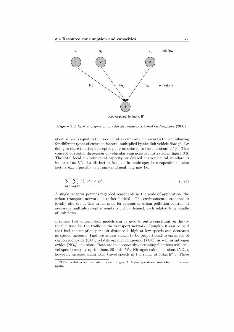
3.4 Resource consumption and capacities 71
1 2 n
q1
q2
qn
1
h q1
h q2
h qn
receptor point, limited to E*
emissions
link flow
Figure 3.6: Spatial dispersion of vehicular emissions, based on Nagurney (2000).
of emissions is equal to the product of a composite emission factor h∗ (allowingfor different types of emission factors) multiplied by the link vehicle flow qv
l . Bydoing so there is a single receptor point associated to the emissions: h∗ qv
l . Thisconcept of spatial dispersion of vehicular emissions is illustrated in figure 3.6.The total local environmental capacity, or desired environmental standard isindicated as E∗. If a distinction is made in mode specific composite emissionfactors hm, a possible environmental goal may now be:
∑
l∈L
∑
m∈Mh∗m qv
lm ≤ E∗. (3.24)
A single receptor point is regarded reasonable as the scale of application, theurban transport network, is rather limited. The environmental standard isideally also set at this urban scale for reasons of urban pollution control. Ifnecessary multiple receptor points could be defined, each related to a bundleof link flows.
Likewise, fuel consumption models can be used to put a constraint on the to-tal fuel used by the traffic in the transport network. Roughly it can be saidthat fuel consumption per unit distance is high at low speeds and decreasesas speeds increase. Fuel use is also known to be proportional to emissions ofcarbon monoxide (CO), volatile organic compound (VOC) as well as nitrogenoxides (NOx) emissions. Both are monotonously-decreasing functions with tra-vel speed (roughly up to about 80kmh−1)8. Nitrogen oxide emissions (NOx),however, increase again from travel speeds in the range of 50kmh−1. These
8Often a distinction is made in speed ranges. At higher speeds emissions tend to increaseagain.
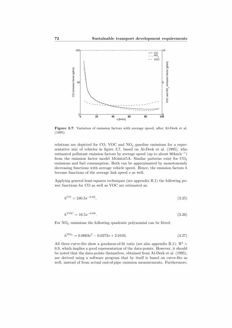
72 Sustainable transport development requirements
0 20 40 60 80 1000
50
100
CO
em
issi
on fa
ctor
[g/k
m]
0 20 40 60 80 1000
5
10
VO
C a
nd N
Ox e
mis
sion
fact
or [g
/km
]
s [km/u]
CONO
xVOC
Figure 3.7: Variation of emission factors with average speed, after Al-Deek et al.(1995).
relations are depicted for CO, VOC and NOx gasoline emissions for a repre-sentative mix of vehicles in figure 3.7, based on Al-Deek et al. (1995), whoestimated pollutant emission factors by average speed (up to about 80kmh−1)from the emission factor model Mobile5A. Similar patterns exist for CO2
emissions and fuel consumption. Both can be approximated by monotonouslydecreasing functions with average vehicle speed. Hence, the emission factors hbecome functions of the average link speed s as well.
Applying general least-squares techniques (see appendix B.1) the following po-wer functions for CO as well as VOC are estimated as:
hCO = 240.5s−0.82, (3.25)
hVOC = 16.5s−0.68. (3.26)
For NOx emissions the following quadratic polynomial can be fitted:
hNOx = 0.0003s2 − 0.0272s + 2.0103. (3.27)
All three curve-fits show a goodness-of-fit ratio (see also appendix B.1): R2 >0.9, which implies a good representation of the data-points. However, it shouldbe noted that the data-points themselves, obtained from Al-Deek et al. (1995),are derived using a software program that by itself is based on curve-fits aswell, instead of from actual end-of-pipe emission measurements. Furthermore,

3.4 Resource consumption and capacities 73
it should be noted that these data-points were derived by simulating route-choice behaviour and environmental effects by introduction of advanced tra-veller information systems (ATIS) focusing on the year 2003. In other words,circumstances in terms of temperature, vehicle mix and age, control measureimplementation etceteras comply with the research objectives of that research,not necessarily this one. However, it is believed that these equations still re-present the right order of magnitude, useful for the type of strategic modellingintended in this research.
Another example for dealing with environmental capacity can be found in theenvironmental capacity oriented urban traffic strategic planning method asproposed by Huapu and Peng (2001), who distinguish a total environmentalcapacity per exhausted gas. Apart from this they also put inspiration out ofthe influential concept of ecological footprint developed by Wackernagel andRees (1995). Ecological footprint is then a sustainability index based on landuse area. It quantifies the intensity of resource consuming related with re-gional bearing capability. In their research, Huapu and Peng (2001), definethe capacity of ecological footprint of an urban passenger transport system asthe environmental capacity, analogue to the use of E∗ in equation (3.24). Li-kewise, in a recent paper by Shresta et al. (2005), a modal split that meetsNOx targets for the city of Beijing, China is determined. Determining the‘available’ environmental capacity on an demarcated urban scale, however, po-ses some challenges, as is discussed in Van Nes (2004), who recently studiedscale-problems in defining and deriving environmental capacity.
An earlier related example is discussed in Immers and Oosterbaan (1991), whodeveloped a model for the calculation of environment-friendly traffic flows inurban networks on the basis of a constrained user-equilibrium assignment. Theconstraints are formulated as a maximum traffic environmental capacity (perroad link) for noise pollution as well as air pollution as compared to standardroad capacity.
In addition, Akinyemi (1998) distinguishes, besides an environmental capaci-ty, also a financial capacity, i.e. unit costs of construction, maintenance andoperation of infrastructure, e.g. cU or link specific unit costs cU
l , multiplied bythe quantity of construction, maintenance and operation at the link levels, Ul,which should not exceed the allocated budget, F ∗, as well as a social capacityconstraint, interpreted as a measure of traffic unsafety per passenger kilometre.These capacities can be equally treated as the mobile emission concept of AnnaNagurney in equation (3.24), for example for the financial capacity:
∑
l∈LcU Ul ≤ F ∗. (3.28)

74 Sustainable transport development requirements
3.4.1 Measures for controlling transition paths
Several transport policy measures can be identified that are used for transportplanning activities, often combined in an integrated approach, in which case awhole range of interventions are applied simultaneously. In an extensive study,described in May et al. (2001), some 60 transport policy measures have beencategorised in five groups, being:
1. Land use measures;
2. Infrastructure provision (for car, public transport, non-motorised trans-port and/or freight specific);
3. Management of infrastructure (for car, public transport, non-motorisedtransport and/or freight specific);
4. Information provision (for car, public transport, non-motorised transportand/or freight specific);
5. Pricing (for car and/or public transport specific).
Through these measures, transport system performance (LOS, mobility, persontravel, accessibility and equity) can be regulated as well as the environmental,financial and social externalities that result.
Furthermore, a distinction can be made between demand-side oriented poli-cies and supply-side oriented policies. For the traditional transport model, inparticular, a few possible regulators, or controls in managing the equilibrationprocess of travel demand and infrastructure supply can be distinguished, basedon the categorisation (between brackets) in table 3.1.
Demand-side options are generally influencing the generalised cost of travel-ling through out-of-pocket costs (affordability), hence controlling total motorvehicle travel demand, by amongst others (TRB, 1997):
• Road use fees and parking tax;
• Vehicle ownership and acquisition taxes;
• Inducements for ride-sharing and tele-commuting.
Supply-side options deal with availability of transport options and capacity inthe transport network, by amongst others (TRB, 1997):
• Investment in public transport and non-motorised transport modes;
• Highway capacity and traffic flow improvements;
• Intelligent Transport Systems (ITS) technology.

3.4 Resource consumption and capacities 75
Table 3.1: Instruments for regulating transport system performance.Demand-side Supply-side
Affordability of transport (5) Availability of transport options (3,4)- fixed travel cost - mode options- variable travel cost - route options
- mode prioritisation- traffic managementRoad capacity (2)- construction- maintenance- mode prioritization
The (effectively) available road capacity to certain modes can be regulatedthrough road construction, pavement maintenance as well as mode prioriti-sation measures. This effective road capacity then influences the generalisedcost of travelling through the travel time. In addition, the number of traveloptions available in combination with the travel time per option influences thecomposite cost of travel. Hence, for example, accessibility can be controlled.


Part II
Modelling sustainableurban transport
development


Chapter 4
Optimisation as a tool forsustainable transport policydesign
4.1 Transport policy and planning
The interaction between travel demand and infrastructure supply is highly com-plex, since both demand and supply comprise of and are influenced by differentand complex as well as interacting processes, as seen in chapter 1. Hence, thechange in a single transport policy measure can be difficult to understand andpredict. Furthermore, the decision-making, leading to these policy measures ispart of another complex process, the policy process.
In this chapter optimisation is discussed as a tool for designing optimal trans-port policies in view of these complex and interacting processes. Optimisationwill (conceptually) prove to be able to assist in the reasoning from a policyobjective to the policy measures taken.
4.1.1 The transport policy process
Transport policy making according to Tolley and Turton (1995) can be defi-ned as ‘the process of regulating and controlling the provision of transport tofacilitate the efficient operation of the economic, social and political life of thecountry at the lowest social cost.’. This implies, amongst others, providingadequate and sufficient infrastructure capacity and efficient operations to bestmeet the current and future needs of the stakeholders involved (those are: inha-bitants, companies, travellers, transporters and/or policy makers). Transportis therefore regulated and controlled through public policy. The level of regula-tion and control, however, may vary from full-state interventions to free-market
79

80 Optimisation as a tool for sustainable transport policy design
Agenda setting
Policy evaluation
Policy
implementaton
Policy formulation
Decision making
Identify
alternatives
Gather and
analyze
alternatives
Apply a decision
tool
feedback
Figure 4.1: The public policy cycle and formulation/decision-making stage.
principles1.
Public policy, which encompasses transport policy, is often depicted as a top-down iterative process, typically including: (1) agenda setting, (2) formulation,(3) decision-making, (4) implementation, and (5) evaluation stages, that movein a linear fashion from higher to lower levels of government. This conceptof political sciences is many times accredited to Lasswell (1951), and depictedschematically in figure 4.1. The first step, agenda setting, is the process bywhich issues come to the attention of policy makers. The second step, policyformulation, is the process in which options are formulated, risks, costs andbenefits are determined, technical evaluation is performed and a ranking ofoptions is made. In the third step, which in some literature is integratedwith the policy formulation step, the decision is made whether one, none or
1The role of free market versus public interest through the state is not discussed in thisthesis, although it will be clear that the conceptualisation of sustainable transport and sub-sequent modelling in this thesis are assuming some kind of regulatory powers, most probablythrough government.

4.1 Transport policy and planning 81
some combination of solutions is selected based on a reasoning from policyobjective(s) to solution(s) or measure(s). This step encompasses the sequentialdecision-making process where: (1) alternatives are identified, (2) alternativesare gathered and analysed, and (3) finally selected with the aid of a decisiontool, as can be seen in figure 4.1 also. It is normally assumed that in thisdecision-making process, technical experts as transport planners come in toparticipate in the decision-making (Barkenbus, 1998). In the fourth step ofpolicy implementation, policies are put into effect. Lastly, the chosen policy ismonitored and evaluated by the authorities themselves as well as the public inthe fifth step of policy evaluation. Final judgement on the success of policiescan then be made.
As said before, much work in transport research is in some way meant to advicepolicy makers taking the third decision-making step2. A role and magnitude ofinvolvement, which is highly dependent on the complexity of transport policyobjectives as well as the adopted decision-making approach, which are discussedin the next paragraph.
4.1.2 Decision-making approaches
Decision-makers are faced with a decision that must be made or a problemthat must be resolved. This is at the heart of policy analysis, which is toevaluate, order and structure incomplete knowledge so as to allow decisions tobe made with as complete an understanding as possible of the current stateof knowledge, its limitations and its implications (Morgan and Henrion, 1990).As there is not such a thing as a single model of decision-making that can beused to guide a planning process in transport, Meyer and Miller (2001), as doOrtuzar and Willumsen (2001), argue that the role and character of the tech-nical transport planning process (basically encompassing the second sequentialdecision-making process in figure 4.1) within transport policy design highlydepends on the decision-making approach followed. Furthermore, the type,context and complexity of the transport problem, as well as the organisationaland political context are dominant in the type of decision-making. In general,three sets of approaches can be distinguished (summarised from Meyer andMiller, 2001; Ortuzar and Willumsen, 2001; Anderson, 2003):
Rational actor or normative decision-making approach Here a rationaland completely informed group of decision-makers is assumed. In thiswell-structured and data-intensive approach, the decision is based onmaximising the attainment of a set of goals and objectives, sometimes ap-plying mathematical programming techniques. Compare also figure 4.1;
Satisficing or behavioural decision approach Here it is assumed that de-cision-makers aren’t completely informed nor are they utility maximisers
2Barkenbus (1998) even argues that transport experts are too much focused on this stepin the policy cycle.

82 Optimisation as a tool for sustainable transport policy design
as in the normative approach, but rather satisficers searching for accepta-ble, though rational, but not necessarily optimal, solutions. Mostly, onlymarginal improvements to the status-quo are made, though still based onsome selection of goals or objectives. Hence, also called incrementalism;
Group decision approaches This group of approaches sees decision-makingas a group learning process with several stakeholders with (different levelsof) decision authority, but diverse goals, values and interests, hence re-flecting organisational or political settings. Negotiation, bargaining andcompromising between groups occurs, through which technically non-optimal solutions often result. Qualitative, quantitative information andforecasts are used to support the overall decision-making process.
Transport models may be applied in all three approaches, in an attempt toprovide analytical insight in the decision-making process. The actual use differsbetween approaches, mainly reflecting the amount of rationality allowed for inthe transport planning paradigm, hence picturing the transport planner froman objective, analytical expert (technocrat) in the normative approach to acommunicative expert with technical knowledge skill (mediator) in the groupdecision approaches3. Transport models can assist in proposing the measurescomplying with the stated goals and objectives. However, transport planners(involved in the technical decision-making stage) do not have a tool for derivingmeasures from an objective readily available. Most transport models can onlyevaluate proposed measures and not derive them from objectives. So, transportplanners themselves will have to come up with an (initial) set of measures that(might) meet the objectives, before a model can be used to evaluate. This canbe a problem if policy objectives become more and more complex; As they do.
4.1.3 Complex transport policy objectives
Most of the goals and objectives4 in transport policy and planning seem veryhard to realise. For example, one can look at the (concept) mobility plan forFlanders, Belgium (Ministerie van de Vlaamse Gemeenschap, 2001) that expli-citly mentions as one of its objectives: ‘The essence of a sustainable mobilitydevelopment is to facilitate the interaction-needs by people and freight thatare a resultant of social and economic activities, through a transport systemin such a way that the demand for mobility can be fulfilled now and in thefuture.’. Three constraints that go with this objective are accordingly posed,assuming:
1. efficient use of scarce resources;3An interesting discussion on transport planning paradigms and the amount and type of
rationality allowed for, is discussed chronologically in Talvitie (1997) and Willson (2001); thelatter one including a comment by Antti Talvitie (Talvitie, 2001).
4The words goals and objectives are used interchangeably here, although one should realisethere are conceptual differences between a goal and an objective. A goal should be seen as theend-result aimed for, whereas an objective is a (quantifiable and) identifiable step towards agoal.

4.2 Transport planning as a design problem 83
2. equity to all groups of users;
3. obeyance of capacity limits of external effects, like safety, liveability aswell as environment.
Plans such as the Flanders mobility plan usually mention a set of traffic andtransport related measures to realise their objectives. However, the proposedmeasures in these plans (in the end) often appear not sufficient to fully meetthe objectives. Transport planning rarely optimises around one objective, usu-ally there are multiple (sometimes contradictory) objectives or even non-viableobjectives.
Goodwin (1999) illustrates this by showing that objectives in transport plan-ning have become increasingly complex, while discussing the whole policy devel-opment from predict-provide approach, to sustainable transport for the Britishtransport policy. He shows that during the decades of predict-provide, theformulation of a suitable policy was easy. The classical four-step transportplanning model gave a prediction of the growth and the suitable policy was tobuild enough roads to provide for it. Every transport planner could formula-te such a policy. But for a sustainable transport system it is less clear whatmeasures have to be taken, when, where and by how much.
Dependent on the decision-making approach chosen, policy analysis can be ap-plied to obtain better insight and understanding on problems with complexobjectives in several ways. Three motivations for this are taken from Morganand Henrion (1990). First, assuming (transport) policy analysis is all abouthaving clearly defined and authorised decision-makers, who have well-definedgoals or objectives as in the normative approach, policy analysis is employedto determine how best to achieve these complex objectives. Secondly, in somecases the alternative policy options are clearly established and the point of ana-lysis is to assist the decision maker in choosing among a discrete or continuousset of options to find the ‘best’ one from the alternatives, as in the satisficingapproach. Thirdly, the possible alternatives are not clearly defined and analysisis used to help the decision maker to identify and explore possible alternativesas well as to choose among them, useful in group decision approaches.
In transport policy analysis, decision makers are also confronted with an incre-asing number of clearly or less clearly defined, interacting as well as complextransport policy objectives and planning restrictions. A transport planningmethod that can assist in determining sets of transport policy measures, whichgive maximum value to these transport policy objectives, hence designing atransport planning, will prove to be useful.
4.2 Transport planning as a design problem
An interesting definition of planning in general is provided by Intriligator andSheshinski (1986) who refer to it as ‘the elaboration of an explicit set of de-

84 Optimisation as a tool for sustainable transport policy design
cisions concerning the present and future values of certain choice variables bya decision maker (planner) in order to achieve certain goals’. Planning accor-ding to them, therefore, involves the determination of a strategy that, in turn,involves decisions on both actions and their timing or pattern of implementa-tion. Relating this to transport planning, which in paragraph 1.2.1 has beencharacterised as both steering the process of allocating traffic generators overspace and time as well as the provision of transport facilities, it is clear that animportant part of (transport) planning is the reasoning from explicit goals andobjectives down to actions over time and space, given some behavioural rules.
Transport planning is as such instrumental to transport policy. Stakeholders,as policy makers, define goals and objectives. The decision maker weightsthese and compares the weighted result with observed reality. Based on thiscomparison, decisions on how to act are made. Hence, the whole process is builton personal assumptions of how policy measures affect reality (Knoflacher et al.,2000), as illustrated in figure 4.2(a). Apparently, some optimisation criterion(goals/objectives like ‘lowest social cost’ or ‘best’) as well as possible measuresor interventions (‘infrastructure capacity’ or ‘efficient operation’ that may beindividually applied or integrated), are inherent to the design of transportpolicy and planning.
Engineering design is an iterative process, where new design proposals aregenerated and evaluated, with the iterative part consisting of synthesis, simu-lation, evaluation and finally decision (Roozenburg and Eekels, 1998). Eachdesign can be evaluated using a simulation model and then compared to somepre-defined goal/objective. If the design does not meet the requirements itis modified and evaluated again in search for the best possible design. Hen-ce, design is essentially optimisation, since optimisation can be defined as ‘theprocedure or procedures used to make a system or design as effective or func-tional as possible, especially the mathematical techniques involved’ (Englishdictionary, 2000).
In transport planning a lot of (technical) knowledge on transport systems isavailable. This knowledge has been formalised in traditional transport modelswith their known predict-provide-manage characteristics. For use in transportplanning, these models are meant to evaluate a-priori, as can be seen in figu-re 4.2(b) as well. The idea of an optimisation model is to use the knowledgeabout transport systems not just to evaluate alternatives, but to design alterna-tives on the basis of some pre-defined goal or objective, as seen in figure 4.2(c).
Mathematically, a policy objective can be seen as a cost criterion that needsto be maximised or minimised. Measures that are to be taken, can be seen asthe input of a certain dynamical system S(T ,W,B). In this system, T is therelevant time axis, W is the signal space and B the behaviour. B is the set oftrajectories that are compatible with the phenomena modelled by the system.The signal space, or manifest variables W can be divided in two parts; first,an input part that can be freely chosen and, second, an output part that is

4.2 Transport planning as a design problem 85
stakeholders
Measures
Decision-maker
Reality Goal/objective
(a) Reality*
Measures
Evaluation
Transport modelPerformance
& effects
Goal/objective
Transport
optimisation
model
Measures,
performance
& effects
(b) Evaluation model
(c) Optimisation model
Compare goal/
objective
* adapted from Knoflacher et al. (2000).
Figure 4.2: (a) Reality*, (b) evaluation modelling versus (c) optimisation in trans-port planning.
completely determined by a given input.
In terms of a transport system S, W is a factor containing variables like thenumber of trips and the travel time. B is a collection of all the possible combi-nations of W, mostly represented by equations. For the transport system, thiscan be a modal split function (as in equation (1.12)) or a cost-flow function (asin equation (1.17)). The input of the system contains the measures that canbe taken to influence the transport system.
The optimal solution is then the input, at which the cost criterion has thehighest value. This way, an optimal package of measures is found to complybest with a certain policy objective, hence a transport planning is designed.Doing so, it is also possible that the model confirms that the system aimed for

86 Optimisation as a tool for sustainable transport policy design
is unrealistic, infeasible or ill conceived. If the optimisation doesn’t converge toa desired system, the concept has to be modified or the problem and alterna-tives reformulated, possibly also resulting in new possible measures, adjustedconstraints or even a different objective function.
Hence, employing control and optimisation techniques to transport planningdesign, can in principle lead to improvements compared to current transportplanning practice. However, there will always be parts in the design anddecision-making process that require human or qualitative judgement, no op-timisation technique can do. The definition of the model equations, objectivefunction as well as constraint values need to be done before the actual opti-misation can take place. This definition phase is prone to errors. At best theoptimisation model outcomes can guide here in the reformulation of equationsand constraints, in other words the input part of the system.
Chapter 5 discusses a dynamic optimisation model in detail. But first some mo-re content will be given to the pro’s and con’s of using optimisation techniquesin transport planning design.
4.2.1 Existing optimisation models
Optimisation techniques have been applied extensively in transport science,although mainly for the purpose of traffic management studies (i.e. advan-ced control techniques for optimal adaptive traffic control), transit studies (i.e.optimal line - and routeplanning in traffic systems) and in logistics (i.e. thetravelling salesman problem). Optimising for the design of tactical or strategictransport plans is done less frequently, although a great body of literature existson traffic assignment techniques (see for an overview on static assignment tech-niques amongst others (Ortuzar and Willumsen, 2001), on dynamic assignmenttechniques (Friesz and Bernstein, 2001), and on transit-assignment (De Ceaand Fernandez, 2001)) as well as transport network design (see amongst othersSteenbrink, 1974; Sheffi, 1985; Bell and Allsop, 1998; Yang and Bell, 1998; Belland Iida, 1999; Nagurney, 2000), which will be discussed in paragraph 4.3.3.Optimisation is also common in the field of transport economics. Few of theseoptimisation models will be mentioned here, as they are illustrative for thedevelopment of general transport optimisation models.
In The Economics of Welfare (c.f. (Pigou, 1932) in Crozet and Marlot (2001)),the economist Arthur Pigou introduced the idea of a congestion toll by comingup with the famous two-road example. This can be seen as the first transportoptimisation model. This approach has been studied extensively and manydifferent models have been made in connection to this idea. Optimal roadpricing measures are the output of these models, and can be seen as the optimalinput for the controlled transport system. An example of such a study can befound in Hau (1992). Timothy Hau presents a model a model that studiesthe theoretical benefits of road pricing based on first economic principles. AsHau’s method is only graphical and is not based on known parameter values, it

4.2 Transport planning as a design problem 87
is perhaps less suitable to a policy maker who wants to formulate an alternativefor a particular transport system.
Indeed most models in transport economics have the problem that they areless suitable for modelling a real world system. A step in the right directionis the model of Yang and Huang (1998), based on the same idea as ArthurPigou’s, but also applicable to a transport network. They present a model foroptimal road pricing for a transport network with some bottlenecks. This is animportant feature for a designer of alternatives. Yet, the model has only oneobjective (welfare maximisation) and one type of measure (road pricing).
Models that can handle more objectives and measures, while still being appli-cable to real world problems as well, are seldom. An example is the modelof De Borger and Wouters (1998). They made a model using static optimi-sation techniques. In relation to transport policy, this model has some usefulcharacteristics. It is meant for a whole country or region, which makes it moresuitable for transport planning. It covers both public and private transport andit calculates optimal prices and capacity for both modes. The model is limitedin two directions. First, it is not a dynamic model, which means that a plan-ning process during some years can hardly be modelled. Second, the networkand causal relations are not modelled explicitly. This means that interpretingthe results for implementation in the real world is not very easy.
The discussion of these three models illustrates what is being looked for, i.e.a model that is easy to interpret, has a direct link to real world transportnetworks, and can cope with different measures and objectives. In chapter 5these characteristics will be derived systematically. It is not strange that exis-ting models do not have these characteristics. Most of them are meant forresearching some policy objective or for finding a theoretical best situation.This is something different from a tool for designing alternatives. Some morediscussion on the implementation of the concept of optimisation in transportplanning will be given in next paragraph.
4.2.2 Transport planning as an optimisation problem
There is, however, some critique to the previously mentioned concept of op-timisation in transport planning. According to Willson (2001) for example,transport planning cannot be characterised as a rational reasoning from an ob-jective to a measure as in optimisation. Richard Willson thus characterises thedecision-making process in transport planning as a group decision approachthat involves negotiation, bargaining and compromising, different from merelyoptimisation. Because of all the political interests involved in the whole processof transport planning, Willson claims it is better characterised as a communi-cative process (Willson, 2001). Therefore, this seems contradictory with therational or normative decision-making approach characterised by optimisation,system dynamics and the linear fashioned policy cycle.

88 Optimisation as a tool for sustainable transport policy design
Also from an engineering design point of view, optimisation can be criticised.Roozenburg and Eekels (1998) studied the design process of objects. For them,designing is a creative process with no single best solution or guaranteed rea-soning resulting in a good design. They show that it is theoretically impossibleto deduct a certain form directly from a certain function. And this deductingis exactly what happens when you are designing through optimisation. Onthe contrary, Andersson (2001), claims (referring to Roozenburg and Eekels(1998)) engineering design is essentially an optimisation problem as long assome human or unquantifiable judgement is allowed for at some stage.
There are many transport experts that criticise the predictive value of trans-port planning models as well. Willson (2001), once more, argues that theseprediction problems make transport models less suitable for transport plan-ning.
Although most of the criticism is right, it is possible to make an optimisationmodel with such properties that it can positively handle most of the comments.Nevertheless, there will always be certain limitations. As long as these limita-tions are respected, the model can well be used in transport planning. Someof the critiques will be discussed in terms of whether they are relevant for theproblem at stake or how they can be avoided.
The first criticism by Willson (2001) is about the policy cycle. The policycycle is based on a rational and powerful policy maker who can dictate thewhole policy process. The rational and powerful policy maker, however, is aseldom case in transport policy. In reality, policy makers have to negotiate withstakeholders and even work together with them as in a group decision process.But even in that case optimisation can be useful. This can be illustrated withtwo cases. First, a leading policy maker with certain objectives surroundedby some reactive, but powerful, stakeholders. The policy maker will try toformulate a policy considering the other stakeholders or formulate a policy co-operating with the other stakeholders. Second, a complex policy surroundingwhere a variable number of stakeholders will co-operate and negotiate, resultingin a certain policy.
In the first case, the policy maker, seen as the leading stakeholder in this pro-cess, will have to come up with a concrete alternative, matching his or hertransport-related objectives. For this, optimisation can be used, in order to besure that the alternative is, given the policy objective, the optimal solution.However, this does not mean that this alternative will be implemented, sinceobjectives and constraints coming from other stakeholders with different inte-rests will have to be considered as well. Looking at the policy cycle this meansthat the phases following the policy formulation are not the exclusive domain ofthe policy maker. The policy makers alternative will have to be evaluated withrespect to all stakeholders’ interests and, depending on the results, probably beadjusted accordingly. In practice this process may be somewhat fuzzier thandescribed, but the main point is that the existence of other stakeholders does

4.2 Transport planning as a design problem 89
not decrease the necessity for a policy maker to formulate alternatives to fulfilobjectives, and optimisation is a good way to do this. Also it makes it easierfor the policy maker to argue his or her alternative and make the causalitiesbetween measures and objectives clear and explainable to the other stakehol-ders. This is especially important when he wants to co-operate with the otherstakeholders rather then considering them as opponents.
In the other case with a group process involving more stakeholders, things arenot really different. All the stakeholders will formulate alternatives accordingto their (most probably complex) policy objectives, possibly considering thereaction of other stakeholders as well. The result of the process will depend onpolitics more than on transport causalities. Nevertheless, all stakeholders willhave to find at least one alternative that fully or partly meets their objective.In the end, a package of measures gets implemented, partly of fully meetingthe stakeholders objectives. So, despite the fact that both the alternativesproposed by a stakeholder and the alternative implemented after the processcan differ from the alternative dictated by the optimisation model, this modelis still helpful in formulating alternatives complying with the objectives aswell as providing an important input to the negotiation process. In some casesmulti-objective optimisation can even be an useful option (see for an interestingdiscussion on this topic Andersson (2001)).
The second criticism, by Roozenburg and Eekels (1998), is on the nature ofthe design process. They consider the design progress as a creative process.A creative process cannot go together with optimisation, they reason. Butthere are some differences between the design problems of Roozenburg andEekels (1998) and the design of a transport planning. The difference betweendesigning, for instance, a water cooker and designing a transport planning isthe number of possible shapes or forms. The design of a chemical plant withone reactor may serve as an example as well. Two raw materials are addedresulting in an output of one product. Temperature and input as well as outputof the raw materials are variable. The design problem is to find a temperaturewith a certain input, the shape or form, resulting in a certain quality andquantity output, its function. Still, there are infinite possible designs, butthe situation is different from designing a water cooker, where the degrees offreedom are far outreaching those for operating the chemical plant. It is thesame with designing a transport policy. The degrees of freedom are limitedby some fundamental points of departure in terms of infrastructure, modes,impedances, land-uses and time. Hence, it must theoretically be possible tomodel close-to-all possible alternatives5 and choose the best one. As can bedone by optimisation.
Taking the reactor and the design problem again, it is clear that this is not thedesign problem according to Roozenburg and Eekels (1998). There is not a lot
5Particularly, when considering strategic modelling, where the alternatives are mostlyspecified in terms of general variables as capacities or prices.

90 Optimisation as a tool for sustainable transport policy design
of creativity in the reasoning from function to form. The specification of thedesign problem results in one optimal alternative.
So, two ways of designing can be distinguished, one with a creative componentresulting in a satisfying, not-necessarily best, design, and one with optimisationresulting in a best design. Related to this, if no suitable alternative is foundin the optimisation process, the designer can be sure there is none; the designproblem formulation might be unrealistic, infeasible or ill-conceived. The onlyoption is then to reformulate the design problem. In the case of Roozenburgand Eekels (1998) it is possible that a functioning form does exist, but thedesigner cannot find it. Another difference is the phase of the modelling in thedesign process. In de case of optimisation, modelling starts before alternativesare formulated. In the case of evaluating, first the design is made, beforethe modelling starts (compare again figure 4.2). Related to this is the factthat in the case of optimisation all possible measures have to be describedmathematically. The key question therefore is whether designing a transportpolicy alternative is more alike Roozenburg and Eekels (1998)’s design problemor more like optimisation.
At first sight transport planning design seems to have more in common withRoozenburg and Eekels (1998)’s design problem. Measures as ramp metering,increase of comfort in public transport, educational programs for drivers, etc.are almost impossible to model as components of a system. Also, the mechanis-ms by which these measures influence the policy objective are difficult or evenimpossible to describe in a mathematical model. But also the design model ofRoozenburg and Eekels (1998) has a phase in which the design has to be mo-delled, i.e. the evaluation phase. This phase is also present in transport policydesign. After designing the alternative, it is evaluated a-priori in a transportmodel. And if the set of measures can be modelled after designing the alter-native it should be possible to do this before. The evaluation of alternativesby modelling is merely done by translating the proposed measures into mo-re generalised or strategic measures that can be implemented in a (strategic)transport model. The measure on ramp metering for example is translated intothe measure road capacity increase. If that can be done, it should also be pos-sible to model the generalised measures in an optimisation model and translatethem into specific measures after the optimisation process. This should workwell because the aim of the optimisation process is to design an alternative andnot to create a blueprint. Hence, it appears to be sufficient to know a certainpolicy direction with system information on for example capacity increases,road pricing, public transport capacity and frequencies and visions for spatialplanning. These kinds of measures can be described in a mathematical model,even in continuous-time, hence containing all possible alternatives.
The third criticism points at the predictive value of transport models in gene-ral. Why optimise when there are serious doubts about the rightness of thedynamics? This problem can be dealt with by looking at other reasons formodelling, apart from predicting. Modelling helps to write down all knowledge

4.2 Transport planning as a design problem 91
and assumptions about transport systems systematically, so that it is inter-nally consistent. For the optimisation model, this results in a system that isconsistent with the way a policy maker looks at the system. The model doesnot claim a perfect prediction. However, it claims that if the assumptions ofthe policy maker are true, the measures will have the predicted results. Aslong as the policy maker realises that the model is only a result of his or herown assumptions, an optimisation model can be used.
The above mentioned comments on the general criticisms on optimisation in(strategic) transport planning have direct consequences for the type and charac-teristics of the optimisation model. These comments are repeated here, but ona somewhat more technical level that is relevant for choosing the form of themathematical model in chapter 5:
Integrated model: The aim of the model is to help with complex causalreasoning from objective to set of measures. The idea is that differentprocesses, interacting and even contradicting with each other, influen-ce these causalities. This means that all relevant traffic and transportrelated processes and their interactions have to be modelled. The onlyrealistic way to do this is to make an integrated model;
Suitable for policy making for real world problems: It is not realisticto ask for models to include all relevant processes for detailed transportnetworks subscribing measures on a similar detailed scale. Nevertheless,the whole exercise is meant to result in an intervention in the real world.This means that the translation from the optimisation result to a realworld intervention must be done without losing validity, perhaps apply-ing hierarchical modelling techniques as will be mentioned in chapter 6.In practice, this will mean that typical characteristics of real world net-works will have to be modelled, but unnecessary details can be avoided.For example, if road pricing is introduced, traffic will relocate to toll-freeroads. This process has to be modelled. But this can be done withoutmodelling a detailed network by making one hypothetical alternative roadif the decision maker is merely interested in quantifying expected toll re-venues. The result is that the effect is clear and plays a role in findingthe optimal solution, but the model stays simple and understandable:
Clear and explainable causalities: In the case of more stakeholders nego-tiating and co-operating to reach a certain transport policy, the stakehol-ders will need to explain their preferred measures and the logic behindtheir ideas. This means that the optimisation model not only has to pro-duce a suitable alternative, but also an explanation why that particularalternative is optimally related to a certain objective. A simple referenceto an optimisation model will of course not be enough. A black box modelwill not be suitable. The causalities should be clear and should be descri-bed without difficult mathematical theory. This does not mean that theprocess of policy making is considered completely rational. It only means

92 Optimisation as a tool for sustainable transport policy design
Problem definition
and demarcation
Solution
principlesModelling
Simulation and
optimisation
Preliminary
design
requirements list concept system model optimised concept
Figure 4.3: The system design process, based on Andersson (2001).
that any stakeholder will connect measures and objectives by causalitiesand want to explain these to other stakeholders. So, a model that helpsto design alternatives should also be capable of giving the correspondingexplanation.
The system design process that results is summarised in figure 4.3. In the pro-blem definition and demarcation phase the design problem and its limitationsare defined and on the basis of this, a list of requirements is made that will beused to generate solution principles, (strategic) design alternatives, or concepts,which will guide the modelling and optimisation phase. In this phase, the de-sign problem is formulated at a sufficient degree of refinement. Simulation andoptimisation are then deployed to predict the properties of the system design.The output is called a preliminary design in order to show these are suggestionsthat still can be altered through human and unquantifiable judgement, or moredetailed at a tactical or operational level of modelling. The output can also bethe reason to reformulate the problem and solution principles.
Referring back to this chapter as well as to chapters 2 and 3, the sustainableurban transport development problem can be defined as a (constrained) op-timisation problem. Next paragraph will discuss modelling and optimisationapproaches for sustainable transport that have been found in literature, beforeproposing a different model in next chapter.
4.3 Methods and models for modelling sustai-nable transport
A classification of existing methods and modelling approaches to sustainabletransport development is discussed in this paragraph. Several approaches canbe found in literature, all having a different perspective on or interpretationof sustainability. Hence, sustainability is weakened here to include some goalor objective for sustainability, which is therefore fundamentally different fromthe standard forecasting approach in transport planning, as discussed beforein paragraph 1.2. The approaches differ in whether they include dynamics intime and whether development trajectories are discerned.

4.3 Methods and models for modelling sustainable transport 93
Present Futuretime
No
Yes
Objective?
Backcasting
Forecasts
Static
optimisation
Dynamic optimisation
Sustainability
indicators
Figure 4.4: Classification of approaches, adapted from Hojer and Mattsson (2000).
Roughly, a distinction can be made between the following four methods andmodelling approaches:
1. Sustainability indicators, which are used to indicate (the deviation from)a target value for a certain sustainability variable or combination ofsustainability variables;
2. Scenario techniques and backcasting, which are concerned with analysingthe future impact of certain scenarios, or backcasting future images (thatcomply with the objective) to the present situation along transition pathsusing scenarios;
3. Static optimisation, which is concerned with optimising transport net-works for a given network topology and travel demand, using variablesas road pricing;
4. Dynamic optimisation, which is used to find transition paths to optimisea transport network over time.
Figure 4.4 illustrates the four different modelling approaches, in relation totraditional forecasting. They are summarised in subsequent paragraphs.
4.3.1 Indicators for transport sustainability
Indicators are central to the monitoring and reporting of progress towardscertain public issues. Collectively indicators can measure the capacity to meetpresent and future needs if it comes to sustainable development or transportsustainability, and therefore has performance-monitoring power. Furthermore,they are often easy to communicate, which is very relevant if it comes to thepolicy process.
Standard use of indicators to measure and monitor transport performance isdone frequently through indicators like level-of-service, traffic speeds, parking

94 Optimisation as a tool for sustainable transport policy design
convenience and price, as well as accident rates per vehicle-kilometre. Formeasuring sustainable transport development, many organisations defined theirindicators related to economic, social and environmental sustainability, liketotal vehicle kilometres, total motorised movement of people and use of fossilfuel energy for all transport, as discussed in length in chapter 2, see for examplethose of The Centre for Sustainable Transportation (CST, 1997) on page 44,also summarised in Gudmundsson (2001) or Litman (n.d.b).
The problem, however, is how to operationalise the use of single indicatorsin indicator systems (the collective of (also interacting) indicators), in otherwords how to measure the ‘overall’ sustainability of a transport system usingindicators. In particular, if many different indicator values exist, amongstwhich some of them even overlap, building indicator systems can become fairlycomplicated.
To obtain an overall sustainability index multi-criteria analysis (MCA) tech-niques can be used. Oude Moleman (2001), for example, shows how this canbe done in practice for analysing and monitoring sustainable transport devel-opment, combining the regime MCA method (using a pairwise comparison ofalternatives), as discussed in Hinloopen et al. (1983), within a Delphi analysis6.The Compass Index of Sustainability is then applied, which clusters indicatorsand assessment scores into different sustainability quadrants. These quadrantsare then superaggregated to produce an ‘Overall Sustainability Index’. Thisindex is inspired by the work of Herman Daly (see for example Daly, 1991) andDonella Meadows (see for example Meadows et al., 1972).
Once established, the index provide clear signals about sustainability perfor-mance over time compared to an absolute or ‘ideal’ future target.
4.3.2 Scenario techniques and backcasting
In order to explore future developments in transport, to experiment with thisfuture and to evaluate possible effects of policy interventions scenario techni-ques can be used. Scenario techniques are well-known forecasting techniques,which according to Malone (2001) assist in structuring, understanding andthinking through a changing situation. Furthermore, do they focus attentionon the structural uncertainty of the most critical factors, as well as increasethe capability of the developers to understand the environment in which thetransport system functions. Scenarios contain an integrated description of thefuture, which pays attention to developments in all factors affecting travel de-mand, but also provide a plausible sequence of events leading to this situation.In addition, an analysis of the present situation and a connection between fu-ture developments and the present situation can be made with such models.An example of the use of scenario techniques can be found in the Dutch Sce-narioExplorer model (Malone, 2001).
6This is a method for structuring communication in a process that allows a group ofindividuals to deal with a complex problem and reach consensus.
4.3 Methods and models for modelling sustainable transport 95
Backcasting is a variation to the scenario techniques and focuses on presentingsolutions to problems that do not seem to be solved, according to conventionalscenarios, trends and forecasts. On the basis of a future image that has beenidentified through a certain vision, for example retrieved by using indicatorassessment as discussed in paragraph 4.3.1, or by using scenarios, which may beobtained through a Delphi analysis, a path between the future image and todayis formulated. Doing so, policy paths towards a certain image are identified, notnecessarily being the optimal paths. In comparison to mathematical modelling,backcasting studies come in when forecasting or optimisation studies indicatethat sustainability targets cannot be met, as depicted in figure 4.4. Hence,backcasting encourages searching for new paths along which development cantake place, particularly when the conventional paths, including those revealedby transport optimisation, do not seem to solve the problem.
Backcasting and forecasting approaches like the scenario approach are com-plementary. The argument Hojer and Mattsson (2000) put forward is thatbackcasting is mainly appropriate where current trends are leading towardsan unfavourable state, so great non-incremental changes are needed. Forecas-ting methods remain necessary because they can inform the backcaster whenbackcasting is required.
Several studies report having used ideas of backcasting for modelling transportsustainability, for example for the Berlin mobility plan in Bluemel (1999), inHojer (1998) for studying the effect of transport telematics on urban transportand environmentally sustainable transport scenarios, reducing emissions by 80-90%, for the EU in Van Wee and Geurs (2000). These studies have beendiscussed in Zuidgeest and Van Maarseveen (2000) as well.
An interesting variation to the use of indicators and backcasting has beenpresented by Miller and Demetsky (1999). They apply regression analysis todetermine land-use limitations (the dependent variable) as a function of thecapacity of the transport system, loaded to a certain level of service (the inde-pendent variable). The capacity of the transport system is measured in termslike number of major through routes in a network, total zonal link volumesor shortest travel distance between zone boundaries and the central businessdistrict.
4.3.3 Optimising transport networks
Optimisation of transport systems is often interpreted as the optimisation oftransport networks in relation to a fixed or an elastic travel demand. Muchliterature deals with the so-called network design problem (NDP), see for anextended review Yang and Bell (1998).
The continuous and discrete network design problem can be distinguished.The continuous network design problem (CNDP) takes the network topologyas given and is concerned with the parameterisations of the network, as can be

96 Optimisation as a tool for sustainable transport policy design
Figure 4.5: Capacity enhancement in the continuous network design problem(CNDP).
seen in figure 4.5. Link parameters that are frequently considered include link(or node) capacity and user charge. CNDP examples are, following Bell andIida (1999):
1. the determination of road width, that is link capacity or number of lanes;
2. the calculation of traffic signal timings;
3. the setting of user charges (e.g. public transport fares and road pricing).
The DNDP is concerned with the topology of the network, see figure 4.6. DNDPexamples are, following Bell and Iida (1999):
1. a road closure scheme;
2. the provision of a new public transport service;
3. the construction of a new road or rail link, a bridge, tunnel or bypass.
Both the CNDP as well as the DNDP are based on the trade-off betweenuser benefit (via travel demand) and the costs of the network alteration (theinfrastructure supply). For example the construction of a bus-lane increases thepublic transport capacity, and therefore public transport throughput, leadingto user benefits. However, the construction costs must be set against the userbenefits. Furthermore, the user (dis)benefits of the non-public transport usersshould also be considered. The same applies to the addition or removal of a linkin the network compared to the costs of the network alteration. The CNDP andDNDP are sometimes combined in the mixed network design problem (MNDP).
In optimal design of networks there are two sets of interest according to Vic-kerman (2001). One is the optimal use of the network by the user (i.c. traveldemand), who is supposed to be minimising his or her individual generalisedcosts of travel. The second is the policy maker or transport network operator,who strives to obtain the most efficient transport network (i.c. infrastructuresupply) for the given travel demand. Hence, transport networks can be desig-ned that may be optimal to the network operator, but deprives users from theiroptimal design (i.c. the shortest path in terms of generalised costs). Hence,advanced optimisation techniques, like static bi-level optimisation and dynamicoptimisation, have been applied in transport planning to serve both interestsin an optimal design.

4.3 Methods and models for modelling sustainable transport 97
Figure 4.6: Adding a link in the discrete network design problem (DNDP).
Static optimisation
Whereas user optimal and operator optimal network designs have individuallybeen the topic of many researches, for example the travelling salesman problem7
in logistics since the 1930s and shortest-path algorithms since the late 1950s, theinteraction between the sets of travel demand and infrastructure supply, seenas two interacting levels of optimising agents only got recognition in the early1970s. Since then the design process is often seen as a bi-level programmingproblem involving an upper-level problem describing the supply problem, anda lower-level problem being the demand problem. Here, the designer/operatorleads, taking into account how the users follow. The leader has prior knowledgeof the responses of the followers, which is also know as a Stackelberg game(Stackelberg, 1934), which is in line with both (possibly contradicting) interestsof the policy maker versus the user as specified by Vickerman (2001). Bi-level formulations have been applied many times in transport research recently,amongst others in traffic control design (see for example Chiou (1999)), trafficassignment algorithms (see for example Jayakrishnan et al. (1995)), origin-destination table estimation (see for example Yang (1995)), road pricing (see forexample Constantin and Florian (1995)) and network design (see for exampleYang et al. (2000)).
The general static bi-level optimisation problem can be expressed mathemati-cally, following Yang and Bell (1998), as:
minv
F (u, v(u))
s.t. G(u, v(u)) ≤ 0,(4.1)
where v(u) is implicitly defined by:
minv
f(u, v)
s.t. g(u, v) ≤ 0,(4.2)
where F and u ∈ U are the objective function and decision or control vectorfor the upper-level decision-maker (the system manager, for example aiming
7Given a finite number of nodes in a network along with the cost of travel between eachpair of nodes, find the cheapest way of visiting all the nodes in the network and returning tothe starting point.

98 Optimisation as a tool for sustainable transport policy design
at minimising the total number of kilometres driven in the network), G isthe constraint set of the upper-level decision vector, f and v are the objectivefunction and decision vector of the lower-level decision-maker (the traveller, forexample aiming at maximising his or her net-utility through route choice deci-sions), and g is the constraint set of the lower-level decision vector. Hence, thelower-level of the bi-level model represents the demand-performance equilibri-um for a given investment action by the user. The whole bi-level NDP is to findthe optimal investment decision-making, for example through optimal capacityimprovement u∗ such that the system objective function F is optimised subjectto a given budget constraint in the upper-level program of equation (4.1), whiletaking account of the reaction of the network users in the lower-level programof equation (4.2).
Applying the static bi-level optimisation techniques to derive sustainable trans-port network can be seen as having an upper-level sustainability goal, whilecomplying with the lower-level behavioural rules of the travellers in the sys-tem. An example of such applications can be found in Yang and Bell (1997),where road pricing is being advocated as an efficient means of managing trafficdemand, while complying with capacity constraints representing other objecti-ves, such as reducing the environmental impact of road traffic and improvingpublic transport. In addition, Kim (1998) presents for example bi-level formu-lations for modelling integrated urban land-use - transport interaction.
Apart from bi-level techniques, network equilibrium techniques, using vari-ational inequality theory, are used to model sustainable transport networks.Variational inequality theory provides a framework for the study of one-levelequilibrium problems, particularly for modelling Wardrop’s First Principle (seeparagraph 1.2.2). For modelling the sustainable transport optimisation pro-blem, variational inequality theory has been extensively applied by Anna Na-gurney, who considers a transport network to be sustainable if ‘the flow patternsatisfies the conservation of flow equations and does not exceed the imposedenvironmental quality standard, subject to the operating behavioural princi-ple’s underlying the network’ (Nagurney, 2000). Transport policies are meantto direct transport networks to sustainability (assuming viability, which imp-lies environmental goals are achievable, given the network, travel demand andenvironmental parameters). Her policies include emission pricing, introductionof tradable pollution permits as well as introduction of new modes. Variationalinequality theory is also used by Paolo Ferrari who also models sustainabletransport networks. In Ferrari (1995) a deterministic variational inequalityequilibrium model for urban transport networks with elastic demand and twotypes of capacity constraints is presented. These capacity constraints can bephysical and environmental. More recently, in Ferrari (1999), a similar study ispresented, modelling a multimodal transport system, subject to some physicaland environmental capacity constraints, as well as budget constraints.
The concept of a sustainable and developing transport systems as definedin paragraph 2.3.1, applying the concept of productive capacity from equa-

4.3 Methods and models for modelling sustainable transport 99
tion (3.7), has been implemented in the Urban Traffic Environmental analysisModel (UTEM). The model has been used extensively for optimising artery’sin several cities, as reported in Zuidgeest et al. (2001) as well as Akinyemiand Zuidgeest (2002). Supply-side interventions are generated iteratively inUTEM to maximise an accessibility criterion based on the productive capacityof the network and generalised costs of travel, while complying with social,environmental and financial resource capacities.
In addition, applying mathematical programming techniques, Huapu and Peng(2001) discuss a static constrained optimisation model for sustainable urbantransport planning. Their model maximises trip making, constrained by anenvironmental capacity parameter for exhausted gasses as well as an ecologicalfootstep capacity8.
Dynamic optimisation
The ‘traditional’ equilibrium models discussed before assume traffic in the op-timal network design is in a static user-equilibrium, and that changes throughdecision variables (for example physical capacity, road pricing etceteras) do notinduce transient effects. However, in view of the characterisation of sustaina-ble urban transport development, a time-varying nature of travel demand andinfrastructure supply in the network seems obvious. Hence, dynamic optimisa-tion models have been introduced that take into account both the time-varyingnature of transport networks as well as disequilibrating effects that changes tothe network may produce, hence reflecting time-lags in adaption processes to-wards the equilibrium put forward in the static models. Furthermore, dynamicmodelling of transport is said to have some additional advantages over staticmodelling as the absence of the so-called temporal Braess paradox, which saysthat sometimes in transport networks paradoxical behaviour may appear, thatis when an enhancement of road capacity results in worse traffic conditions forall road users (Bell and Iida, 1999). Furthermore, the unrealistic sequentialnature of the traditional transport planning model and the lack of feedbackseem better treated by dynamic versions of this model (as recalculations of thetraditional models occur each time-step). In addition, dynamic optimisationallows for determining the paths of control variables and state variables for thedynamic disequilibrium system over a finite or infinite time horizon to maxi-mise an objective function. Hence, dynamic optimisation is also called optimalcontrol.
Dynamic optimisation models for optimising transport networks have first beenpublished by Friesz and Fernandez (1979), who developed a linear optimal con-trol problem in order to determine optimal maintenance policies, knowing thatthe quality of a road facility is determined by natural factors, rate of use andmaintenance investments, whereas the demand for the road facility is again
8Ecological footprint is an index of sustainable development based on land-use area. Itquantifies the intensity of source consuming related with the regional bearing capability. Afamous introduction in the concept is given in Wackernagel and Rees (1995).

100 Optimisation as a tool for sustainable transport policy design
assumed to be a function of its quality under these circumstances. An earlyexample of optimising transport networks is given in Steenbrink (1974), whoapplied heuristic iterative optimisation methods to derive bi-level optimisationproblems in transport network design. Nijkamp and Reggiani (1988) deri-ved a dynamic model that represents the evolution of an integrated spatialinteraction system. Friesz and Shah (1998) discuss the theory of disequilibri-um network design and use this in a model to maximise social welfare in atransport system. Donaghy and Schintler (1994) ibid. Donaghy and Schintler(1998), as does Lensink (2002), study the possibility of using optimal controltechniques for modelling infrastructure management in terms of road capacityenhancements, and road/parking pricing. On a strategic level the EuropeanCommission ‘Optimisation of policies for transport integration in metropolitanareas (OPTIMA)’ study, as reported by European Commission (1998) ibid. Pf-affenbichler and Shepherd (2002) or Pfaffenbichler (2003), tested several (pre-defined) packages of sustainable transport measures in a dynamic transportmodel against two objective functions (an economic efficiency function as wellas a sustainability objective function), hence finding optimal policy packagesapplying multidimensional minimisation techniques, instead of optimal controltechniques.
In the sustainable urban transport development concept presented in this re-search a methodology is proposed that uses a standard forecasting frameworkin which goals are explicitly defined. Hence, it operates partly in the highligh-ted area of figure 4.4. Backcasting techniques should be applied when standardtransport policy measures cannot somehow lead to the desired targets. Inother words, if non-incremental changes, perhaps introducing new means oftransport, are needed.
Next chapter discusses dynamic optimisation in more detail and will introducean optimal control model based on the concept of sustainable urban trans-port development. This model can be used as a tool for designing sustainabletransport policies.

Chapter 5
A dynamic optimisationmodel for sustainable urbantransport development
5.1 Introduction
Optimisation is part of everyday life. For example, when dealing with scarceresources, as road space or environmental capacity, one would like to optimisethe use of it. Several optimisation techniques exist for different types of op-timisation problems (Naidu, 2003); for example static optimisation problems,when confronted with controlling a system under steady-state conditions, ga-me theoretic problems, when multiple actors are optimising individually withinone system, dynamic programming problems, when dealing with multiple stageproblems (preferably in discrete-time) in the sense that at each set of times,a decision can be chosen from a finite number of decisions based on some op-timisation criterion, or stochastic problems, where the nature of the signalis stochastic, etceteras. Deterministic, single stage optimisation problems incontinuous-time can be treated as dynamic optimisation problems. Dynamicoptimisation is concerned with the optimal control of systems under dynamicconditions, i.e. the system variables are changing with respect to time andthus time is included in the differential or difference equations describing thesystem.
In this chapter, dynamic optimisation is used to model sustainable urban trans-port development in accordance with the characterisations and theory devel-oped in previous chapters. First, some basics on dynamic optimisation aregiven. Followed by a detailed description of the dynamic transport model thatis solved applying the Maximum Principle of Pontryagin, which is discussedand demonstrated accordingly.
101

102 A dynamic optimisation model
S
C
Controller
System
Control input u(t)
State x(t) Output y(t)
Reference
input r(t)
Figure 5.1: The general control configuration.
5.2 Dynamic optimisation
In general control theory a controller C is determined that will cause the (non-linear) dynamic system S(T ,W,B), as characterised in paragraph 4.2, which isdescribed in terms of state equations x(t) to satisfy some physical constraintsand at the same time maximise or minimise a chosen performance index J .The system output y(t) is controlled through the control input u(t), which isdriven by the state equations and some reference signal or input r(t), which isillustrated in figure 5.1 as a so-called closed-loop control.
In optimal control, a control u∗(t) is looked for that will drive the system S fromthe initial state (at time t0) to a final state (at time t1) with some constraints onthe controls and states, while at the same time minimising or maximising thegiven performance index J , which is some function of the system output y(t)as well as controls u∗(t) over time.
The formulation of the optimal control problem therefore requires (Naidu,2003):
1. a mathematical description of the system to be controlled;
2. a specification of the performance index J ;
3. a statement of boundary conditions and physical constraints on the statesand/or controls.
If a nonlinear ordinary differential system with initial conditions for the statevariable x(t), also equation of motion or transition, is considered:
dx(t)dt
= f(x(t), u(t), t), x(t0) = x0, (5.1)
with the control variable u(t), which like the state variable x(t), may be boun-ded by some equality or inequality constraint:

5.2 Dynamic optimisation 103
g(x(t), u(t), t) ≥ 0, (5.2)
then the performance index, or cost criterion or functional, J , can be formulatedas a so-called Bolza-problem1:
J = F (x(t1), t1)) +∫ t1
t0
H(x(t), u(t), t)dt, (5.3)
where x(t) is the solution of equation (5.1) at time t, F is some final state,which may be fully, partially fixed or free; also called transversality condition.Furthermore, there is some (piecewise) continuous function H. The final time t1may be fixed or free also.
The optimal control problem for a minimisation problem can be stated asthe determination of the control function u∗(t), given system equation (5.1),constraints (5.2) and cost criterion (5.3), such that:
J∗ = J(x0, u∗(t), t) ≤ J(x0, u(t), t), ∀ u(t). (5.4)
Dynamic programming (sometimes referred to as Bellman’s Optimality Prin-ciple) and Pontryagin’s Maximum Principle are two basic tools for studyingoptimal control theory, and can be found in any textbook on optimal control.Dynamic programming determines a closed-loop optimal control that is optimaleverywhere, whereas the open-loop Maximum Principle refers only to quanti-ties along a specific trajectory. However, to obtain the optimal control usingdynamic programming one has to discretise a high dimensional state space,which causes an exponential growth of the number of grid points with dimen-sionality (referred to as the curse of dimensionality). Computational methodsbased on Pontryagin’s Maximum Principle avoid this curse of dimensionality.Given the very large dimensionality of transport network state spaces, it isbelieved here that computational methods based on the Maximum Principleare more promising than the methods based on dynamic programming, and ishenceforth applied here. First, the nature of the applied model equations aswell as the dynamic transport model itself are discussed, before turning to adescription of the Maximum Principle in paragraph 5.4.
5.2.1 Continuous-time modelling
Dynamic optimisation techniques can be formulated in continuous-time as wellas discrete-time. In discrete-time, a period of time t ∈ N is divided into nintervals of length T, so time is indexed as xt. In continuous-time t ∈ R in theinterval [t0, t1], so a variable is a function of time x(t). Although the world is
1A number of variations to general class of Bolza-problems exist, for example the Mayer-problem if H = 0, or Lagrange-problem if F = 0 in equation (5.3).

104 A dynamic optimisation model
observed in discrete-time only, it is often much easier to work with continuous-time.
A few main arguments are postulated in favour of the use of continuous models:
1. Although individual strategic planning decisions are generally made atdiscrete time-intervals, it is difficult to believe that they are co-ordinatedin such a way as to be perfectly synchronised; they will overlap in time insome way. As the variables that are usually considered and observed arethe outcome of a great number of decisions taken by different operators atdifferent points in time, it seems natural to treat the different processes asif they were continuous (Gandolfo, 1993). This also takes away the needto make a decision on what is the appropriate ‘natural’ unit of time, wheretime is expressed in for example: T = 1[month], or: T = 1[quarter];
2. A specification in continuous-time is particularly useful for the modellingof disequilibrium adjustment processes like for example the inducementof travel demand (see chapter 3);
3. The availability of a model formulated as a system of differential equationsenables its user to get forecasts and simulations for any time-interval, andnot only for the time unit inherent in the data;
4. Continuous-time specifications are more tractable mathematically andmore consistent with growth-theory frameworks and diffusion models.Hence, they also provide a better way of depicting ongoing aggregatebehaviour (Donaghy and Schintler, 1998);
5. The state of transport systems is one which is continuously evolving (seechapter 1);
6. Development in itself is a dynamic, continuous phenomenon, thereforealso the strategic development of a transport system (see chapter 2).
In this research a continuously evolving state of the transport system is mo-delled that can be observed at regular intervals. Therefore the state of thetransport system can be determined at these time intervals.
5.2.2 Disequilibrium modelling
Optimising agents after calculating the optimal value of some decision varia-ble, cannot immediately adjust the actual to the desired value due to frictionsand imperfections of various types (Gandolfo, 1997). Hence, it is questionablewhether a static equilibrium, i.e. ‘a transport system finds itself in an essenti-ally timeless state where system users are either unable or unwilling to changetheir behaviour’ (Bell and Allsop, 1998), exists. At best a transport systemis near equilibrium, or tending towards it, only prevented by external factors.To include time-lagged processes, as reaction times or habitual chances, partialadjustment equations can be used. In a partial adjustment equation, indicating

5.2 Dynamic optimisation 105
a discrepancy between the desired and actual value of a variable, this processcan be modelled. The actual value is then adjusted towards the desired valueonly gradually, according to a coefficient of reaction or speed of adjustment.
Disequilibrium modelling can be illustrated using an equation in discrete-time,following Gandolfo (1997). When the value of y at time t ∈ N depends on thepresent and past values of some other variable x, a distributed-lag equation isused, which in discrete time (n time periods) can be written as:
yt = b0xt + b1xt−1 + · · ·+ bnxt−n, (5.5)
where b0, b1, · · · , bn are known nonnegative constants, with:
n∑
i=0
bi = b. (5.6)
Often this series bi is declined geometrically for some: 0 < k < 1, as in:
bi = kbi−1. (5.7)
Hence, equation (5.6) changes to:
b =∞∑
i=0
bi = b01
1− k. (5.8)
The equivalent continuous-time formulation to equation (5.5) is:
y(t) =∫ ∞
0
[f(t′)x(t− t′)] dt′, (5.9)
which is a convolution equation, also called a continuously distributed-lag equa-tion. The function f(t′) is called a weighting function, which may be:
∫ ∞
0
f(t′)dt′ =1b, (5.10)
or an exponential weighting function, analogue to equation (5.7):
f(t) = γe−γt, (5.11)
hence, equation (5.9) can be written as:
y(t) =∫ ∞
0
γe−γt′x(t− t′)dt′. (5.12)

106 A dynamic optimisation model
It can be shown that this equation is equivalent to a partial adjustment diffe-rential equation in continuous-time, i.e.:
dy(t)dt
= γ (x(t)− y(t)) . (5.13)
For a proof, the reader is further referred to Gandolfo (1997).
The coefficient of adjustment γ can be interpreted as the reciprocal of themean time-lag, which is the time required for about 63% of the discrepancybetween y(t) and x(t) to be eliminated by changes in y(t), following a changein x(t). The mean time-lag is defined as:
t =∫ ∞
0
t′f(t′)dt′, (5.14)
which is equivalent to:
t = γ
∫ ∞
0
t′e−γt′dt′ =1γ
, (5.15)
for the exponential weighting function: f(t) = γe−γt. So, when: lim γ →∞, themean time-lag tends to zero, which means that y(t) adjusts to x(t) immediately.
The partial adjustment equation (5.13) can be used in the specification of dy-namic disequilibrium models. In this type of models, it is claimed that thedynamic system is continuously adjusting to the partial equilibrium x(t), forexample due to some positive external influence F+, but effectively is in a di-sequilibrium y(t), except when the system is in a steady-state, which is shownin figure 5.3. This is different from an instantaneous adjustment as depicted infigure 5.2. In terms of transport, this can be seen as the time lagged adjustmentof travel demand to changes in exogenous social-economic factors, but also tochanges in infrastructure supply. Referring to Manheim’s equilibrium, as de-picted in figure 1.5, the equilibrium point is aimed for, but due to the systemdynamics and time-lags the transport system is said to be in a disequilibriumstate continuously. As time is passing several positive and negative externalinfluences F will change the disequilibrium, which is illustrated in figure 5.4.Basically, the disequilibrium process guides the transport system from one par-tial equilibrium state to another, perhaps eventually reaching a steady state,the static equilibrium.
Disequilibrium transport network design models have not been used widely. Assaid before, applications can be found in transport network design, i.e. Frieszand Shah (1998), Donaghy and Schintler (1994) ibid. Donaghy and Schintler(1998).

5.2 Dynamic optimisation 107
t
t2
t1
External factor F+
New equilibrium
Old equilibrium
t0
Figure 5.2: Instantaneous adjustment to an external factor F+ (De la Barra, 1989).
Old equilibrium
t
t2
t1
External factor F+
New equilibrium
time lag
t0
Figure 5.3: Dynamic lagged adjustment to an external factor F+ (De la Barra,1989).
t1
F-
Old equilibrium
t0
t
New equilibrium
t2
t3
F+
F+
t4
t5
Partial equilibrium
Figure 5.4: Dynamic lagged adjustment to several external factors F .

108 A dynamic optimisation model
5.3 A dynamic transport optimisation model
In this paragraph an optimal control model for sustainable urban transportdevelopment is derived. The equations are formulated as such, to prepare forthe use of the Pontryagin’s Maximum Principle, which is the topic of parag-raph 5.4. The dynamic model is based on the conceptual ideas set forward inchapter 2, where sustainable urban transport development has been defined,and chapter 4, where sustainable transport planning has been characterised asan optimisation problem. The basic model equations are based on the traditi-onal transport planning model equations from chapter 1 as well as the sustai-nability requirements from chapter 3. Summarising, the dynamic model canbe characterised by its:
Dynamics The transition paths in time towards a sustainably developed trans-port system are described by state variables representing traffic performance(flow, capacity, condition) and impacts (emissions, throughput, kilometres tra-velled) per road link in the network as well as the costate variables with thesestate variables representing the marginal costs;
Optimisation The nature of the problem of designing a sustainable transportplanning is that of a constrained optimisation problem. Different transportpolicy objectives are translated into cost functions over time (the planninghorizon), i.e. maximising accessibility, maximising person throughput or mini-mising vehicle congestion, which can be studied and compared;
Controls Transport improvements are related to travel time savings and vehi-cle operating costs savings, hence affecting generalised costs of travelling. Theimprovements can be effected through controls to the decision maker: engi-neering interventions (road construction, road maintenance, public transportpriority) as well as pricing measures (vehicle taxes, parking taxes, bus fares);
Constraints The optimisation and use of controls are limited by (endpoint)constraints, i.e. environmental and financial capacities the decision maker hasto comply with at the end of the planning horizon, but also constraints thatphysically limit the control value or state value over time.
The basic idea behind this dynamic optimisation model is that a transportplanner who, confronted with some transport policy objective as well as several(endpoint) constraints or resource capacities (like infrastructure budget, envi-ronmental capacity and equity objectives), has at stake, different (combinationsof) transport measures or controls, like new construction, road maintenance aswell as pricing that will change the effective road capacity and productivecapacity of the network, hence affecting traffic performance. The compositegeneralised costs, consisting of vehicle-operating-costs as well as travel timefor the different modes on different routes, will influence accessibility, whichis also dependent on the interaction potential between zones (the trip genera-tion capacity). From this the total elastic mode-specific travel demand, and

5.3 A dynamic transport optimisation model 109
consequently traffic flows, can be determined on the basis of the equilibrationprocess of travel demand and infrastructure supply. Available resources areconsumed from the resource capacities available. This general structure of thedynamic transport model can be depicted as a diagram with causal relations,see figure 5.5.
Among the transport system attributes in the model are things as route specifictravel times, travel costs and capacities (at some reference condition or duringthe period when traffic is heaviest, i.e. during peak hours). These are attributesobserved at points on a continuum of time, necessary for medium and longterm strategic transport planning purposes, not to be confused with short-termdynamics of (for example) non-recurrent traffic congestion.
The basic idea behind the optimal control models discussed here are inspiredby the work of Laurie Schintler and Kieran Donaghy, as published in Donaghyand Schintler (1994) ibid. Donaghy and Schintler (1998). Similar models havebeen reported in Buttler and Shortreed (1978), Friesz and Fernandez (1979)and Lensink (2002).
In the next paragraphs, the specific elements of the dynamic model are discus-sed, subdivided into dynamic models for travel demand, infrastructure supplyand system induced effects in paragraph 5.3.1, transport planners objectivefunctions in paragraph 5.3.2 as well as constraints in paragraph 5.3.3.
5.3.1 Transport dynamics
In the optimal control model, transport dynamics are expressed using a set ofordinary differential equations. The main state variables x(t) are travel demandV (t), using a disequilibrium formulation as discussed in paragraph 5.2.2, as wellas infrastructure supply, or link capacity C(t). Furthermore, some other statevariables representing the transport induced effects, i.e. vehicle-kilometres tra-velled K(t), person- throughput P (t) and total emissions E(t) are formulated.Each state variable is discussed subsequently.
The spatial structure of the transport network is represented using subscript in-dices with the different variables. Let the graph G(N ,L) be a transport networkwith nodes n ∈ N and links l ∈ L. The link set is: L = 1, 2, · · · , l, · · · , L ∈NNl . Each link may have several attributes, such as length, free-flow speed, ca-pacity, road type etceteras. The centroid-set: Z = (I,J ) ⊂ N , is a subset of Nand consists of origins i, numbered: I = 1, 2, · · · , i, · · · , I ∈ NNi , as well asdestinations j, numbered: J = 1, 2, · · · , j, · · · , J ∈ NNj . Similarly, a mode-set can be defined as: M = 1, 2, · · · ,m, · · · ,M ∈ NNm , whereas the route-set between origin-destination pair (i, j) is: Rij = 1, 2, · · · , r, · · · , R ∈ NNr .Social-economic population segmentation is equally represented in a set: K =1, 2, · · · , k, · · · ,K ∈ NNk . A pollutant set: P = 1, 2, · · · , p, · · · , P ∈ NNp ,is defined as well. Finally, a control set: U = 1, 2, · · · , u, · · · , U ∈ NNu ,contains all possible control options.
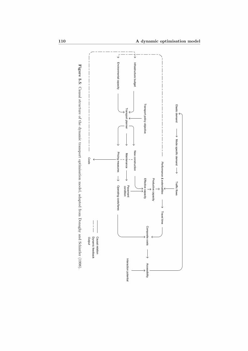
110 A dynamic optimisation model
Infrastructure budget
Environmental capacity
Transport p
lanner
New construction
Maintenance
Pavement
condition
Pricing measures
Operating costs/fares
Productive capacity
Effective capacity
Accessibility
Performance & externalities
Travel tim
e
Composite costs
Mode specific demand
Traffic flows
Elastic demand
Costs
Causal relation
Dynamic feedback
Output
Interaction potential
Transport policy objective
Fig
ure
5.5
:C
ausa
lstru
cture
ofth
edynam
ictra
nsp
ort
optim
isatio
nm
odel,
adapted
from
Donaghy
and
Sch
intler
(1998).

5.3 A dynamic transport optimisation model 111
0 5 10 15 20600
650
700
750
800
850
900
950
1000
time
Vl(t
)
γ = 0.25γ = 0.5γ = 1
Figure 5.6: The changing state of travel demand for different values of γ1.
A disequilibrium travel demand model with static trip generationcapacity (A1)
Disequilibrium equation (5.13) can be used to model the changing state of traveldemand V (t) on a road link over time t. If the trip generation capacity Qis fixed (for simplicity Q is denoted here in [pcuh−1] instead of [persh−1]),the dynamic travel demand model can be written as a first-order ordinarydifferential equation:
dV (t)dt
= γ1 (Q− V (t)) . (5.16)
The solution to this equation obviously is:
V (t) = Q + (V0 −Q)e−γ1(t−t0), (5.17)
where V0 is the initial state for V (t) at: t = t0(= 0). The solution2 is graphicallydepicted in figure 5.6 for different values of the adjustment coefficient γ1, while:Q = 700pcuh−1 and: V0 = 1000pcuh−1. For relatively small relaxation time,implying high γ1 the disequilibrium system moves quickly from V0 to Q.
A disequilibrium travel demand model with time-varying trip gene-ration capacity (A2)
Exogenous explaining (or independent) social-economic or land-use variablesmight influence the dependent trip generation capacity Q over time, hence
2A variable-step continuous solver ODE45 based on an explicit Runge-Kutta (4,5) formulais used in Matlab.

112 A dynamic optimisation model
0 5 10 15 20
700
800
900
1000
1100
1200
time
Q(t
)
x1(t)
x2(t)
Q(t)
Figure 5.7: Dependent Q(t) and independent exogenous variables x1(t), x2(t), pa-rameters: α1 = 0.7, α2 = 0.3, and: α3 = 0.
creating a time-varying Q(t), which can be calculated by constructing a linearmultiple-regression equation:
Q(t) =nk1∑
k1=1
(αk1xk1(t)) + αk1+1 , (5.18)
with in total nk1 exogenous explaining variables in vector ~x(t), with parametervector ~α and αk1+1 as the intercept. An example of Q(t) is given in figure 5.7,with time-varying (arbitrary chosen) explaining variables x1(t) and x2(t), forexample representing the number of households as well as average monthlyincome. The values of x1 and x2 vary over time, and therefore the dependentvariable Q(t) varies accordingly.
Now the dynamic travel demand equation (5.16) changes to:
dV (t)dt
= γ1 (Q(t)− V (t)) , (5.19)
of which the solution is:
V (t) = e−γ1(t−t0)
(V0 + γ1
∫ t′1
t′0
Q(t′)eγ1t′dt′)
, (5.20)
with V0 the initial state for V (t) at t = t0(= 0). The solution is graphicallydepicted in figure 5.8 for different values of the adjustment coefficient γ1, while:V0 = 1000pcuh−1. It can be observed that for a high: γ1 = 10, implying smallrelaxation time, the exogenous Q(t) from figure 5.7 is retrieved.

5.3 A dynamic transport optimisation model 113
0 5 10 15 20
700
800
900
1000
1100
1200
time
Vl(t
)
γ = 0.25γ = 1γ = 10
Figure 5.8: The changing state of travel demand for different values of γ1.
A disequilibrium network travel demand model with time-varyingtrip generation capacity (A3)
In a transport network, link travel demand is dependent on the choice-behaviourof the trip maker. Furthermore, several origins, destinations, modes and routesexist. Therefore, the time-varying trip generation capacity in an origin-zone i isdistributed over several destinations j, modes m and routes r. To capture thischoice-behaviour the four-step model equations from paragraph 1.2 can be usedto replace Q(t) in equation (5.19) and find the equilibrium traffic flow Vl(t) forlink l at time t.
Doing so, a disequilibrium formulation, following Donaghy and Schintler (1998),expresses the changing state of travel demand (in [pcuh−1]) between the equi-librium traffic volume Vl(t) and actual traffic volume Vl(t). Depicted again asa dynamic travel demand model this reads:
dVl(t)dt
= γ1
(Vl(t)− Vl(t)
), ∀ l. (5.21)
The equilibrium link demand function Vl(t) is assumed to be built-up of:
1. the time-varying trip generation capacity of a zone i, based on social-economic characteristics of the zone, Qi(t);
2. a simultaneous mode m, destination j and route r choice model, Gijmr(t).
The generated trips Qi(t) in zone i are distributed over the different choice-options using a discrete-choice model Gijmr(t) and converted to vehicles in[pcuh−1] applying a vehicle-occupancy factor θ1m:

114 A dynamic optimisation model
Vl(t) =∑
i∈I
∑
j∈J i
∑
m∈M
∑
r∈Rlij
θ1m (Qi(t) Gijmr(t)) , ∀ l, (5.22)
withRlij the route serving origin-destination pairs that contain link l, or: Rl
ij =r ∈ Rij | ∃n : rn = l, and: r = (1, 2, · · · , lr, · · · , Lr) ∈ NNr , as well as J i
the destination set excluding destination j = i, or: J i = j ∈ J | @n : jn = i.The trip generation per zone is expressed as a linear multiple-regression equa-tion, being a slight variation to equation (5.18):
Qi(t) =nk1∑
k1=1
(αk1ixk1i
(t)) + αk1+1i, ∀ i. (5.23)
The chances of simultaneously selecting a certain destination j, mode m androute r are obtained using a dynamised version of the doubly-constrained gra-vity model of equation (1.19), which is distributing trips on the basis of theutilities uijmr(t) for the different mode m, and route r choice-combinations aswell as the time-varying trip attraction value Xj(t):
Gijmr(t) =Xj(t) exp(−λ1uijmr(t))∑
j′∈J i
∑m′∈M
∑r′∈Rij′
Xj′(t) exp(−λ1uij′m′r′(t)), ∀ i, j,m, r,
(5.24)
with scale parameter λ1.
The destination attractiveness Xj(t) is equally expressed as the trip generationcapacity:
Xj(t) =nk2∑
k2=1
(αk2j xk2j (t)
)+ αk2+1j , ∀ j, (5.25)
with nk2 the number of exogenous explaining variables in vector ~xk(t), withparameter vector ~αk and αk2+1j as the intercept.
The utility function uijmr(t) for generalised costs of travel is expressed as alinear equation of route travel time τr(t) and route travel cost κijmr(t)3, similarto equation (1.1):
3Often, but not here for reasons of simplification, travel costs are weighted to an incomeparameter if a population segmentation k ∈ K is considered, hence the second term in
equation (5.26) changes to β4mκijmr(t)
α2πk, with πk the income-level for segmentation k and α2
some kind of time-value-of-money parameter, see for example Odoki et al. (2001).

5.3 A dynamic transport optimisation model 115
uijmr(t) = β3mτr(t) + β4mκijmr(t), ∀ i, j, m, r, (5.26)
with β3m and β4m mode-specific parameters. Parameter β3m is the value-of-time parameter for conversion of time to monetary units. Similarly β4m canbe expressed as the time-value-of-money parameter for conversion of money totime units.
Route travel time is a summation of link travel times that comprise route r,which are expressed as strictly increasing, continuous and nonlinear functionsof the volume Vl(t) to effective capacity Ce
l (t) ratio and free-flow travel time τ0l ,
by applying equation (1.17) :
τr(t) =Nr∑
lr=1
τ0lr
1.0 + α1
(Vlr (t)Ce
lr(t)
)β1 , ∀ r, (5.27)
with parameters α1 and β1.
Route travel costs are similarly expressed as a function of the exogenous time-varying vehicle operating costs om as well as distance dependent vehicle taxcontrol Uv(t) and a parking tax control at the destination Up
j (t) (a flat tariffis assumed)4:
κijmr(t) = (om + θ2mUv(t)) dr + θ2mUpj (t), ∀ i, j, m, r, (5.28)
with parameter θ2m representing the conversion of imposed taxes to the vehicle-type m, in other words the disutility per vehicle-type.
The route distance is accordingly calculated as:
dr =Nr∑
lr=1
dlr , ∀ r, (5.29)
where dl is the length of link l, and Nr the number of links comprising router ∈ Rij .
The solution to this model now is:
Vl(t) = e−γ1(t−t0)
(Vl0 + γ1
∫ t′1
t′0
Vl(t′)eγ1t′dt′)
, ∀ l, (5.30)
4In fact, the subscript i could be omitted here as it is not part of the function itself,because each r is determined by a unique combination of i, j, and m. For reasons of claritythe utility and alike remain, however, indicated with subscripts i, j, m, r.

116 A dynamic optimisation model
0 5 10 15 20
700
750
800
850
900
950
1000
1050
1100
1150
time
Vl(t
)
123
Figure 5.9: The changing state of travel demand in a small network.
with Vl0 the initial state for Vl(t) at: t = t0(= 0). This solution is illustratedin figure 5.9 for a three-link network (assuming one origin, one destination,and one mode), where the, fixed, effective link capacity: Ce
1(t) < Ce2(t) <
Ce3(t), hence activating the route-choice r only. The adjustment coefficient is:
γ1 = 0.25, while the initial states are: V1(0) = V2(0) = V3(0) = 1000pcuh−1.The time-varying exogenous trip generation capacity Qi(t) is the same as inprevious example (see figure 5.7).
A disequilibrium network elastic demand model with time-varyingtrip generation capacity (A4)
If travel demand is regarded to be elastic to changes in accessibility, as discussedbefore in paragraph 3.3.1, the equilibrium level Vl(t) should also include ameasure of elasticity.
This implies that not necessarily all trip generation capacity (still based on thesocial-economic and land-use characteristics of the zone) is revealed per se. Inother words, the potential trip generation capacity of a zone needs to be known.
Starting with the disequilibrium travel demand model:
dVl(t)dt
= γ1
(Vl(t)− Vl(t)
), ∀ l, (5.31)
the equilibrium link demand function Vl(t) is now assumed to be built-up of:
1. the time-varying potential trip generation capacity of a zone i, based onsocial-economic characteristics of the zone, Qi(t);

5.3 A dynamic transport optimisation model 117
2. a demand elasticity factor Dij(t), representing the induced effect of ac-cessibility between zones i and j on trip generation;
3. a simultaneous mode m, destination j and route r choice model, Gijmr(t).
Hence, part Dij(t) of the time-varying potential trip generation capacity Qi(t)in zone i is distributed over the different mode and route choice-options for thecorridor (i, j), using a discrete-choice model Gijmr(t) and converted to vehiclesin [pcuh−1], applying a vehicle occupancy factor θ1m, as before:
Vl(t) =∑
i∈I
∑
j∈J i
∑
m∈M
∑
r∈Rlij
θ1m
(Qi(t) Dij(t) Gijmr(t)
), ∀ l. (5.32)
The general structure of the trip generation potential Qi(t) is similar to equa-tion (5.23), while the simultaneous discrete-choice model Gijmr(t) is equal toequation (5.24), hence they are not repeated here.
The maximum amount of revealed travel demand on a corridor (part of it mayactually go to another destination j, as seen in equation (5.24)), or origin-destination pair (i, j) will now be: Qi(t) · Dij(t), where the elasticity factorDij(t) is a slight variation to equation (3.19), i.e.:
Dij(t) = a1 + b1 exp(−λ2
(c∗ij(t)− c0
ij
)), ∀ i, j, (5.33)
with c∗ij(t) the composite costs of travel, a1 the minimum ratio of trips (ofQi(t)) that will be performed irrespective of the composite costs and (a1 + b1)the maximum ratio, i.e. 100% of the trips that can be performed at idealcircumstances, or free-flow conditions, which is at c0
ij .
The composite cost, or logsum cost, on a origin-destination pair (i, j) arecalculated by aggregating generalised costs (expressed in the utility functionuijmr(t), which is equation (5.26)) over all modes m and routes r that serve theorigin-destination pair, analogue with equations (3.20) to (3.22), while beingmade time-dependent:
c∗ij(t) = − 1λ3
ln
∑
m∈M
∑
r∈Rij
exp(−λ3uijmr(t))
, ∀ i, j, (5.34)
where λ3 is the scale parameter to obtain the expected maximum utility of thechoice-set: C = (Rij ,M).
The ‘free-flow’ composite costs c0ij can be derived by calculating the generali-
sed costs for all choice-options under free-flow conditions, and applying equa-tion (5.34) once.

118 A dynamic optimisation model
The general solution to this model is similar to the solution of previous model,i.e.:
Vl(t) = e−γ1(t−t0)
(Vl0 + γ1
∫ t′1
t′0
Vl(t′)eγ1t′dt′)
, ∀ l, (5.35)
with Vl0 again the initial state for Vl(t).
A dynamic infrastructure supply model with capacity control (B1)
Travel time on a road link is directly related to the supply of infrastructure, inother words the capacity available to the trip maker, as expressed through thevolume-over-capacity (Vl/Ce
l ) ratio in for example equation (1.17).
From this it is obvious that the performance of a road link in terms of thevolume-over-capacity ratio can be improved by expanding the capacity of theexisting road link:
dCel (t)dt
= U cl (t), ∀ l, (5.36)
where U cl (t) is a continuous control variable u(t) for new capacity with dimen-
sion [pcuh−1T−1]5. Hence, U cl (t) is changing the functionality of the road link
as in the continuous network design problem (CNDP), as discussed in parag-raph 4.3.3, figure 4.5.
A dynamic infrastructure supply model with capacity control andnatural deterioration (B2)
Infrastructure that is in existence will loose quality at a constant rate ξ1 intime. This natural deterioration can be due to climatological reasons as wellas average known wear by vehicles on the infrastructure. The deteriorationfactor can be determined on the basis of the design life of the pavement. Ifthe total deterioration due to these factors is linear with the existing capacity,equation (5.36) can be rewritten as:
dCel (t)dt
= U cl (t)− ξ1C
el (t), ∀ l. (5.37)
Assuming that the autonomous deterioration can be counteracted partly byconducting pavement maintenance, another control variable u(t), representingthe rate of maintenance Um
l (t), can be added to equation (5.37):
5The dimension of Ucl (t) is [pcuh−1 T−1], if T is the time-unit of integration, which may
be months or years in the case of strategic modelling.

5.3 A dynamic transport optimisation model 119
dCel (t)dt
= U cl (t)− (ξ1 − Um
l (t)) Cel (t), ∀ l, (5.38)
which is:
dCel (t)dt
= U tl (t)− ξ1C
el (t), ∀ l, (5.39)
when including the general capacity enhancement variable U tl (t) for construc-
tion and maintenance as a control variable u(t):
U tl (t) = U c
l (t) + Uml (t)Ce
l (t), ∀ l, (5.40)
following Lensink (2002).
The solution to this equation obviously is:
Cel (t) = e−ξ1(t−t0)
(Ce
l0 +∫ t′1
t′0
Ul(t′)eξ1t′dt′)
, ∀ l, (5.41)
with Cel0 the initial state for effective capacity Ce
l (t).
A dynamic infrastructure supply model with capacity control andmaintenance (B3)
The effective link capacity can be seen as a function of the design capacityCd
l (t) and pavement condition Il(t):
Cel (t) = α3
Cdl (t)
Il(t)β5, ∀ l, (5.42)
with parameters α3, a scaling parameter to convert link condition units tocapacity units and β5, the pavement condition elasticity for effective capacity.This equation is derived from Haas and Hudson (1978), who first related designcapacity and pavement condition to effective capacity. Obviously, at perfectpavement condition, that is when: Il(t) = Ip, or: α3/Iβ5
p = 1.0.
Here, the design capacity Cdl (t) is the capacity as constructed, thus assuming
perfect maintenance level, and can be changed due to new construction, asbefore in equation (5.36):
dCdl (t)dt
= U cl (t), ∀ l. (5.43)

120 A dynamic optimisation model
6 8 10 12 14 16 18 2020
40
60
80
100
120
140
s [k
m/h
]
[m/km] IRI
CarsUtility vehiclesBusesLight trucksMedium/heavy trucks
Figure 5.10: Maximum speeds as function of roughness IRI.
The functional performance of a road pavement Il(t) relates to the degree ofserviceability of the pavement over time, usually indicated as ride quality orroughness. Roughness is readily noticed by road users because of its immediateimpact on the riding comfort. It may also be perceived by its influence on fuelconsumption.
To illustrate the effect of roughness on the performance level, figure 5.10 showsmaximum speeds as function of roughness, expressed through the InternationalRoughness Index (IRI), for a study in Brazil, as mentioned in Paterson (1987).
This International Roughness Index Il(t) is an international standard used tomeasure pavement roughness and is based on an open-ended scale from zero fora true planar surface, increasing to about 6 for moderately rough paved roads,12 for extremely rough paved roads with potholing and patching, up to about20 for extremely rough unpaved roads, as discussed in Paterson (1987).
As is also done in for example BTE (1996) a deterministic approach involvingdetermining pavement performance by a function, which is directly relating pa-vement condition to variables as traffic volume, measures of pavement strength,pavement age and environmental factors, is applied here.
An empirical formula to predict the roughness progression Rl(t) is then, follo-wing Paterson (1987):
Rl(t) = w exp(v t)(1 + Sl)β6 Wl(t), ∀ l. (5.44)
The road roughness increases due to climate factor v, road type w, the modifiedstructural number Sl, with factor β6, and through wear (in 106 [axlesyear−1]).

5.3 A dynamic transport optimisation model 121
The wear Wl(t) on a road link is due to traffic volumes and an equivalentstandard axle load factor (ESAL), Φ1m, per vehicle type m, which is:
Wl(t) = α4
∑
i∈I
∑
j∈J i
∑
m∈M
∑
r∈Rlij
Φ1mθ1m
(Qi(t) Dij(t) Gijmr(t)
), ∀ l. (5.45)
Parameter α4 converts the peak hour axle loads to an equivalent daily or yearlymeasure (remember that the state variables represent peak hour conditions on-ly). The equivalent standard axle load factor per vehicle type m is exogenouslyderived. Parameter ϕmy is the average load on an axle y by vehicle type m, ϕS
y
is the standard single axle load of axle group y and ρ1 the axle load equivalencyexponent:
Φ1m =∑m
(ϕmy
ϕSy
)ρ1
, ∀ m. (5.46)
The modified structural number, Sl, of the road link is exogenously derived:
Sl = 0.40 log10 TDl + 3.0, ∀ l, (5.47)
where TDl is the amount of design traffic that goes with the design capacity Cd
l .
Combining these, the change in road condition Il(t) is modelled due to wear,i.e. roughness due to axle loading and climatological effects, Rl(t), as:
dIl(t)dt
= γ2Rl(t), ∀ l, (5.48)
which can be controlled by applying the following control function Ml(t) to themaintenance ‘gap’ (I − Ip), which is:
Ml(t) = α5(Il(t)− Ip)Uml (t)β7 , ∀ l, (5.49)
where Ip is the perfect pavement condition (Ip = 2mkm−1 IRI), Uml (t) is the
control variable known as a pavement overlay and α5 and β7 are parameters.
Equation (5.49) can be derived from experimental results described in Colucci-Rios and Sinha (1985), who found that the relationship between rate of reduc-tion in roughness R and resurfacing through overlay thickness Um (in theirpublication in [inches]) is:
∆R = −α5 (Um)β7 , (5.50)
with: α5 = 0.61 and: β7 = 0.26.

122 A dynamic optimisation model
Logically, the following dynamic equation can now be constructed:
dIl(t)dt
= γ2 (Rl(t)−Ml(t)) , ∀ l. (5.51)
Furthermore, natural deterioration using factor ξ1 can be introduced again,similar to equation (5.37). In addition, Donaghy and Schintler (1998) suggest(for such equation) that the link maintenance level should be corrected for therelative pavement improvement (seen over a cross-section of the road link) dueto capacity expansion. For better understanding both processes are introducedexplicitly writing the trajectory for Il(t) over time interval (t0, t1). Also, ad-justment coefficients γ2 are applied to delay the contributions of the differentprocesses:
Il(t1) =Il(t0) + γ2
∫ t′1
t′0
Rl(t′)dt′ + γ2ξ1
∫ t′1
t′0
Il(t′)dt′ − γ2
∫ t′1
t′0
Ml(t′)dt′
− γ2α6
∫ t′1
t′0
(Il(t)− Ip)U c
l (t′)Cd
l (t′)dt′, ∀ l,
(5.52)
with weight parameter α6. After taking the time-derivative this yields:
dIl(t)dt
= γ2
(Rl(t) + ξ1Il(t)−Ml(t)− α6(Il(t)− Ip)
U cl (t)
Cdl (t)
), ∀ l. (5.53)
System induced effects
The travel demand and infrastructure supply dynamics discussed in previousparagraphs will influence the transport network performance over time. Hence,it seems logical to introduce some dynamic equations that measure the inducedeffects of the disequilibrium transport dynamics.
In this model the system induced effects are related to the ‘aggregated’ disequi-librium level Vl(t) only. For explicitly deriving system induced effects it should,however, be possible to make a distinction in vehicle-type m and possibly al-so in population segmentation k. To do so, separate state variables Vlmk(t)will have to be defined. This would, however, imply a too large increase ofm × k times as many state-variables as well as costate variables. Hence, herethe system induced effects are first calculated at the disaggregate mode andpopulation segmentation level, before being accumulated into the equilibriumlevel Vlt.
The change in person-throughput P (t) on a route, as discussed in parag-raph 3.2.2, can be modelled as:
dP (t)dt
= γ1
(P (t)− P (t)
). (5.54)

5.3 A dynamic transport optimisation model 123
Person throughput. as discussed before in paragraph 3.2.2, in the transportnetwork is calculated as the number of person trips made (so leaving out thevehicle occupancy factor θ1m) on all routes r multiplied by the speed of move-ment sr(t):
P (t) = α4
∑
i∈I
∑
j∈J i
∑
m∈M
∑
r∈Rij
(Qi(t) Dij(t) Gijmr(t) sr(t)
), (5.55)
with α4 a parameter to convert the peak-hour traffic to an equivalent daily oryearly person-throughput, and where the speed is:
sr(t) =dr
τr(t), ∀ r. (5.56)
The dimension of P (t) is in [perskmh−2], since P (t) is a continuous variable ascompared to P∆t
r in equation (3.4), which is measured over a period of time ∆t,hence has dimensions [perskmh−1].
The total number of kilometres K(t) driven in the transport network can bederived similarly as P (t), that is:
dK(t)dt
= γ1
(K(t)−K(t)
), (5.57)
with the disequilibrium ‘mileage’ being:
K(t) = α4
∑
i∈I
∑
j∈J i
∑
m∈M
∑
r∈Rij
θ1m
(Qi(t) Dij(t) Gijmr(t)
)dr. (5.58)
To calculate the total non-point emissions for pollutant p ∈ P as discussed inparagraph 3.4, another dynamic equation is used:
dE(t)dt
= γ1
(E(t)− E(t)
). (5.59)
The disequilibrium level of emissions E(t) is calculated as the number of modespecific trips multiplied with a mode and pollutant-specific emission factor εm|p,link length dl and a speed factor (that assumes emissions are lower at higherspeeds in network), using parameter β8m|p, following equation (1.22) by Ziets-man (2000), which is also applied in Kim and Hoskote (1983), with parametervalues given in equations (3.25) to (3.27):
E(t) =α4
∑
i∈I
∑
j∈J i
∑
m∈M
∑
r∈Rij
∑
lr∈r
θ1m
(Qi(t) Dij(t) Gijmr(t)
)
εm|p dlr
(dlr
τlr (t)
)−β8m|p
,
(5.60)

124 A dynamic optimisation model
with link travel times as before:
τl(t) = τ0l
[1.0 + α1
(Vl(t)Ce
l (t)
)β1]
, ∀ l. (5.61)
Equation (5.60) is formulated for use of one, possibly dominant, pollutant typeonly, for example introducing a composite emission factor. If one wants toinclude several types of pollutants an extra summation over p ∈ P is required.
5.3.2 Transport policy objectives
In an optimal control formulation the so-called equations of motion for the statevariables x(t), which are discussed in previous paragraph, are controlled by thecontrol variables u(t) as to minimise or maximise a certain cost criterion J .These cost functions represent (combinations of) transport policy objectives,which are accordingly formulated in terms of transport system performanceor movement needs. Hence, the sustainable transport system requirementsmentioned in chapter 3 can be reformulated as cost criterions in the optimalcontrol model.
A cost criterion for controlling traffic performance (C1)
As the policy maker wants to focus on the actual movement of vehicles in trans-port systems, a cost criterion that is directly related to measures of congestion,or level-of-service seems appropriate.
Hence, the cost criterion could be formulated as to keep or bring the level ofservice for a road link or all links in the network at a certain volume-over-capacity level δl over the time horizon (t0 − t1), which is, following Donaghyand Schintler (1998):
min∫ t1
t0
∑
l
(Vl(t)Ce
l (t)− δl
)2
dt =
max−∫ t1
t0
∑
l
(Vl(t)Ce
l (t)− δl
)2
dt.
(5.62)
The implication of this cost criterion is that the control paths are chosen assuch that all existing infrastructure is used homogenously, that is links with alow volume-over-capacity level will increasingly used to reach level δl, whereasthe contrary applies to links with a high volume-over-capacity level.
A cost criterion for controlling accessibility (C2)
When a policy maker wants to focus on the interaction opportunities of peoplethe accessibility concept by Sales Filho (1998), as discussed in paragraph 3.2.3could be used, also including the theory on composite costs.

5.3 A dynamic transport optimisation model 125
This accessibility cost criterion aims at minimising composite costs between the
origin-destination zone pairs that have highest attraction value:√
Qi(t)Xj(t),hence maximising over the time horizon (t0 − t1):
max∫ t1
t0
∑
i∈I
∑
j∈J i
(Qi(t)Xj(t)
) 12
exp(−β9c
∗ij(t)
)dt, (5.63)
where β9 is a parameter, Qi(t) and Xj(t) are exogenous variables for correctedorigin and destination attractiveness, as in equations (3.10) and (3.11), andc∗ij(t) is the composite cost of travel between zones i and j, which is equati-on (5.34):
c∗ij(t) = − 1λ3
ln
∑
m∈M
∑
r∈Rij
exp(−λ3uijmr(t))
, ∀ i, j. (5.64)
The implication of this cost criterion obviously is that resource allocation isdirected at relatively attractive origin-destination pairs (i, j).
A cost criterion for controlling person-throughput (C3)
If the focus of transport policy is on the available network capacity to accom-modate quick and comfortable movement of persons by the existing modes oftransport, the person throughput over time could be aimed at, i.e. maximisingperson throughput in the transport network over the time horizon (t0 − t1):
max∫ t1
t0
P (t) dt, (5.65)
which is equal to the productive capacity of the transport network CP in[perskmh−2], analogue to equation (3.7). The person-throughput P (t) is cal-culated using equation of motion (5.54).
The implication of this cost-criterion is amongst others that modes with a highvehicle-occupancy factor θ1m are given most resources.
A cost criterion for controlling equity (C4)
When equity is considered by the policy maker, the composite costs of travellingbetween an origin and destination for the different population segmentations kshould be roughly equal, as expressed before in equation (3.16).
Hence, for k ∈ K segmentations, the equity level that should be aimed at isminimising the mean deviation:

126 A dynamic optimisation model
min∫ t1
t0
∑
i∈I
∑
j∈J i
(1K
∑
k∈K| Qi|k(t) c∗ij|k(t)− c∗ij(t) |
)dt =
max∫ t1
t0
−∑
i∈I
∑
j∈J i
(1K
∑
k∈K| Qi|k(t) c∗ij|k(t)− c∗ij(t) |
)dt,
(5.66)
over the time horizon (t0−t1), with c∗ij(t), as before, being the weighted averagecomposite costs of travel on origin-destination pair (i, j) for all populationsegmentations k, which is:
c∗ij(t) =1K
∑
k∈K
(Qi|k(t) c∗ij|k(t)
), ∀ i, j, (5.67)
while, the composite costs of equation (5.34) are now segmentation k dependentas well, that is:
c∗ij|k(t) = − 1λ3|k
ln
∑
m∈M
∑
r∈Rij
exp(−λ3|kuijmr|k(t))
, ∀ i, j, k. (5.68)
and, the production potential share for segment k:
Qi|k(t) =Qi|k(t)∑
k′∈K Qi|k′(t). (5.69)
However, for computational reasons, which are discussed later on, equati-on (5.66) is better written in terms of quadratic deviation from the averagesegmentation specific composite costs at t = t0, which is:
max∫ t1
t0
−∑
i∈I
∑
j∈J i
(∑
k∈KQi|k(t) c∗ij|k(t)− c∗ij(t0)
)2
dt. (5.70)
The replacement of c∗ij(t) with c∗ij(t0) is done to obtain a more stable objectivefunction and basically implies that deterioration from the average initial levelof equity is not allowed.
The general implication of this cost criterion is that preference is given to seg-mentations k that experience relatively high composite cost, though irrespectiveof the interaction opportunities at the origin and destination zones.
As mentioned before, a more equitable or levelled distribution of transportopportunities to the different segmentations results from this policy objective.

5.3 A dynamic transport optimisation model 127
The weighted average composite costs acting as a source-term, could howeveralso imply that investments are only directed at levelling the absolute deviationtowards zero only. An overall improvement of the transport system somehow isnot reflected in this measure; only the distribution of transport opportunities.
Note that to calculate this cost criterion, obviously, also the demand modelneeds to be changed, in order to allow for k different population segments,which is:
Vl(t) =∑
i∈I
∑
j∈J i
∑
m∈M
∑
r∈Rlij
∑
k∈Kθ1m
(Qi|k(t) Dij|k(t) Gijmr|k(t)
), ∀ l. (5.71)
5.3.3 Measures and bounds
In the previous paragraphs several policy control measures u(t) have been used.For each of the control variables it is common, even necessary in the case oflinear controls, to pose inequality bounds on their values.
For the new construction control variable U cl (t) a lower and upper bound (say
land-use limitation, i.e. space available for expanding capacity) can be formu-lated as follows:
0 ≤ U cl (t) ≤ U c
lmax, ∀ l. (5.72)
Likewise the pavement overlay control Uml (t) is bounded by a lower and upper
bound (say technical limitation).
0 ≤ Uml (t) ≤ Um
l (t)max, ∀ l. (5.73)
The upper bound Uml (t)max, in the case of model (B3), varies with time as it
is not possible to improve IRI beyond perfect pavement condition Ip, which is:
Il(t)− Ip+
γ2
(Rl(t) + ξ1Il(t)− α5(Il(t)− Ip)Um
l (t)β7 − α6(Il(t)− Ip)U c
l (t)Cd
l (t)
)= 0, ∀ l,
(5.74)
or:
Uml (t)max =
Il(t)− Ip + γ2
(Rl(t) + ξ1Il(t)− α6(Il(t)− Ip)
Ucl (t)
Cdl (t)
)
γ2α5(Il(t)− Ip)
1β7
, ∀ l.
(5.75)

128 A dynamic optimisation model
Both controls U cl (t) and Um
l (t) may also be bounded by an exogenously deter-mined budget constraint F ∗(t). If the standard price for construction cost iscc1 money units and for maintenance cost cm
2 money units, this is:
∑
l
(cc1dlU
cl (t) + cm
2 dlCdl (t)Um
l (t)) ≤ F ∗(t). (5.76)
This budget constraint may also be formulated as an isoperimetric or integralequality or inequality constraint (see also paragraph 5.4.1):
∫ t1
t0
∑
l
(cc1dlU
cl (t) + cm
2 dlCdl (t)Um
l (t))dt = F ∗t1 , (5.77)
which can then be written as:
dF (t)dt
=∑
l
(cc1dlU
cl (t) + cm
2 dlCdl (t)Um
l (t)), (5.78)
with F (t) being the integral expenditure. The boundary points for F (t) are:
F (t0) = 0, F (t1) ≤ F ∗t1 . (5.79)
Both linear tax controls Uv(t) and Upj (t) should be bounded by inequality
constraints as well:
0 ≤ Uv(t) ≤ Uvmax, (5.80)
and:
0 ≤ Upj (t) ≤ Up
jmax
, ∀ j. (5.81)
Furthermore, pure state constraint may be applied to the emissions E(t) as well.The environmental capacity E∗ is then the exogenously determined maximumtotal emissions at any time t:
E(t) ≤ E∗. (5.82)
Likewise, the emission constraint can be written as an integral inequality con-straint:
∫ t1
t0
E(t) dt ≤ E∗t1 , (5.83)

5.4 Pontryagin’s Maximum Principle 129
which can then be written as:
dE(t)dt
= E(t), (5.84)
with E(t) being the integral emissions. The boundary points for E(t) are:
E(t0) = 0, E(t1) ≤ E∗t1 . (5.85)
Alternatively, a pure state constraint at the endpoint may be applied to theemissions E(t1). The environmental capacity E∗
t1 is then the exogenously de-termined maximum total emissions at time t = t1:
E(t1) ≤ E∗t1 . (5.86)
Summarising, a model has been described consisting of travel demand dyna-mics and infrastructure supply dynamics, where infrastructure is controlledthrough construction and maintenance and demand through vehicle taxes andparking taxes. In the meantime some system effects (as vehicle kilometres,person throughput and total emissions) are monitored. The controls are se-lected as such as to maximise (or minimise) the transport objective function.These controls are constrained by physical, financial or technical bounds. Theemissions as well as budget are bound over time or at the end of the planninghorizon t1 and should not exceed a certain value, while at the same time themodel is trying to optimise the objective. Hence, a dynamic optimisation mo-del is described that can be solved for example using Pontryagin’s MaximumPrinciple.
5.4 Pontryagin’s Maximum Principle
Optimal control was originally developed in the Soviet Union by Lev Pontryaginand others in the early 1960s (Pontryagin et al., 1962) and has been appliedin both technical sciences (often as minimisation problems, like fuel control forsoft landing of a rocket on the moon) as well as in social, medical and economicsciences (for example maximising the effectiveness of drugs treatment). A basicset of necessary conditions for optimal control is named Pontryagin MaximumPrinciple, shortly Maximum Principle, or in the case of minimisation problems,Minimum Principle.
Besides the Maximum principle, another popular approach to optimal control iscalled dynamic programming as developed by Richard Bellman, which is basedon the principle that given the fact that an optimal path has the property thatwhatever the initial conditions and control values are (over some initial peri-od), the control over the remaining period must be optimal for the remaining
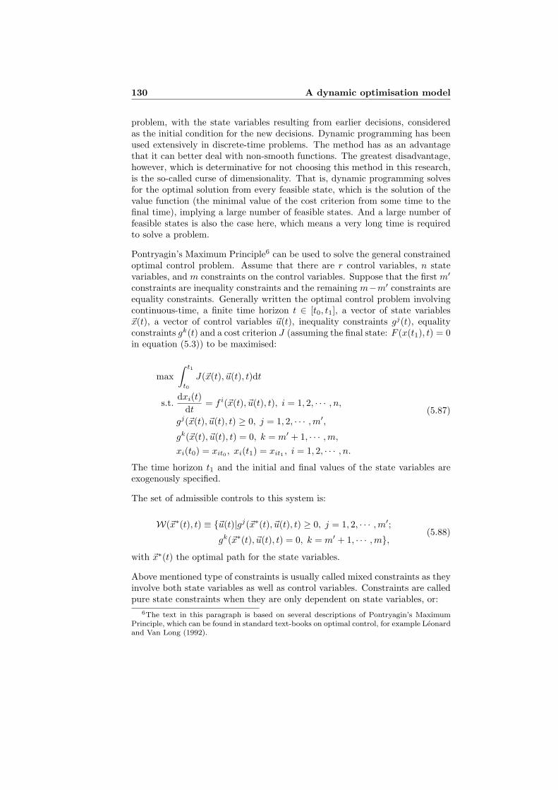
130 A dynamic optimisation model
problem, with the state variables resulting from earlier decisions, consideredas the initial condition for the new decisions. Dynamic programming has beenused extensively in discrete-time problems. The method has as an advantagethat it can better deal with non-smooth functions. The greatest disadvantage,however, which is determinative for not choosing this method in this research,is the so-called curse of dimensionality. That is, dynamic programming solvesfor the optimal solution from every feasible state, which is the solution of thevalue function (the minimal value of the cost criterion from some time to thefinal time), implying a large number of feasible states. And a large number offeasible states is also the case here, which means a very long time is requiredto solve a problem.
Pontryagin’s Maximum Principle6 can be used to solve the general constrainedoptimal control problem. Assume that there are r control variables, n statevariables, and m constraints on the control variables. Suppose that the first m′
constraints are inequality constraints and the remaining m−m′ constraints areequality constraints. Generally written the optimal control problem involvingcontinuous-time, a finite time horizon t ∈ [t0, t1], a vector of state variables~x(t), a vector of control variables ~u(t), inequality constraints gj(t), equalityconstraints gk(t) and a cost criterion J (assuming the final state: F (x(t1), t) = 0in equation (5.3)) to be maximised:
max∫ t1
t0
J(~x(t), ~u(t), t)dt
s.t.dxi(t)
dt= f i(~x(t), ~u(t), t), i = 1, 2, · · · , n,
gj(~x(t), ~u(t), t) ≥ 0, j = 1, 2, · · · , m′,
gk(~x(t), ~u(t), t) = 0, k = m′ + 1, · · · ,m,
xi(t0) = xit0 , xi(t1) = xit1 , i = 1, 2, · · · , n.
(5.87)
The time horizon t1 and the initial and final values of the state variables areexogenously specified.
The set of admissible controls to this system is:
W(~x∗(t), t) ≡ ~u(t)|gj(~x∗(t), ~u(t), t) ≥ 0, j = 1, 2, · · · ,m′;
gk(~x∗(t), ~u(t), t) = 0, k = m′ + 1, · · · ,m, (5.88)
with ~x∗(t) the optimal path for the state variables.
Above mentioned type of constraints is usually called mixed constraints as theyinvolve both state variables as well as control variables. Constraints are calledpure state constraints when they are only dependent on state variables, or:
6The text in this paragraph is based on several descriptions of Pontryagin’s MaximumPrinciple, which can be found in standard text-books on optimal control, for example Leonardand Van Long (1992).
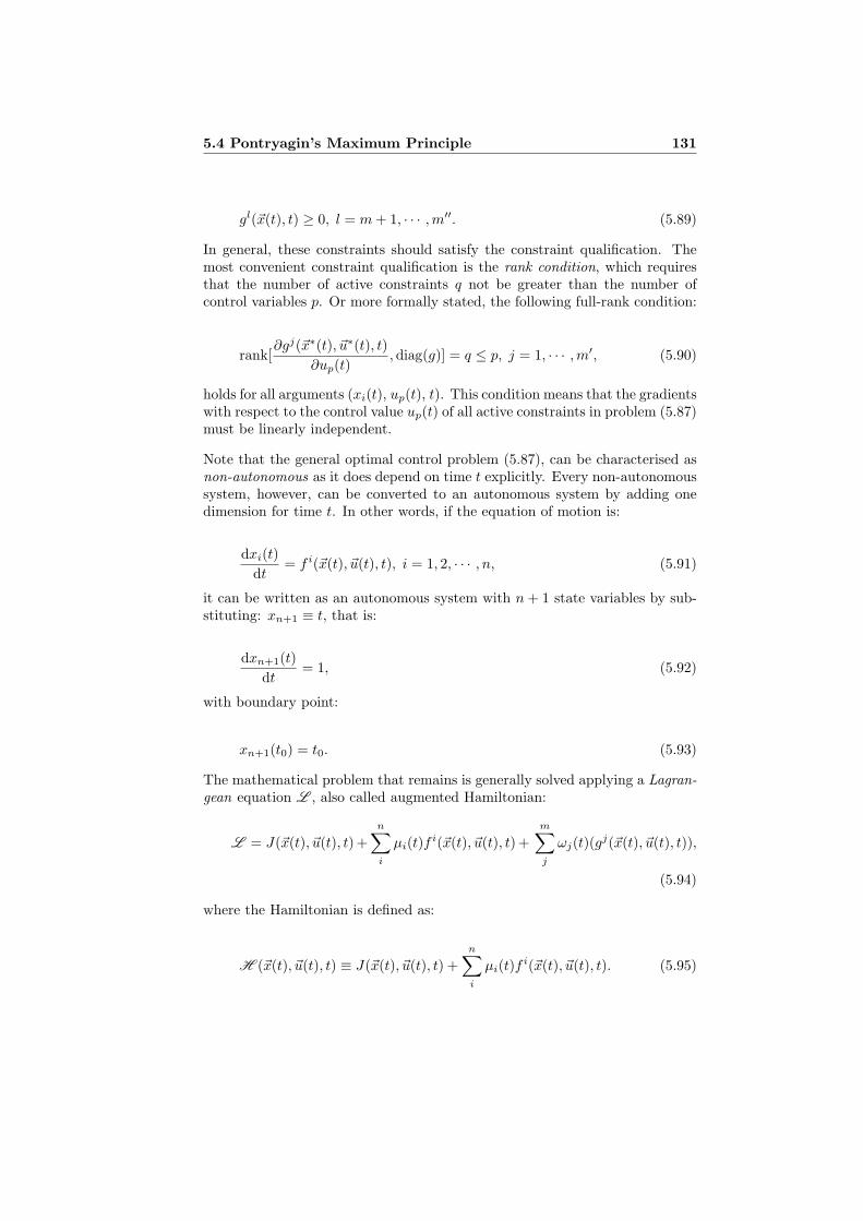
5.4 Pontryagin’s Maximum Principle 131
gl(~x(t), t) ≥ 0, l = m + 1, · · · ,m′′. (5.89)
In general, these constraints should satisfy the constraint qualification. Themost convenient constraint qualification is the rank condition, which requiresthat the number of active constraints q not be greater than the number ofcontrol variables p. Or more formally stated, the following full-rank condition:
rank[∂gj(~x∗(t), ~u∗(t), t)
∂up(t), diag(g)] = q ≤ p, j = 1, · · · ,m′, (5.90)
holds for all arguments (xi(t), up(t), t). This condition means that the gradientswith respect to the control value up(t) of all active constraints in problem (5.87)must be linearly independent.
Note that the general optimal control problem (5.87), can be characterised asnon-autonomous as it does depend on time t explicitly. Every non-autonomoussystem, however, can be converted to an autonomous system by adding onedimension for time t. In other words, if the equation of motion is:
dxi(t)dt
= f i(~x(t), ~u(t), t), i = 1, 2, · · · , n, (5.91)
it can be written as an autonomous system with n + 1 state variables by sub-stituting: xn+1 ≡ t, that is:
dxn+1(t)dt
= 1, (5.92)
with boundary point:
xn+1(t0) = t0. (5.93)
The mathematical problem that remains is generally solved applying a Lagran-gean equation L , also called augmented Hamiltonian:
L = J(~x(t), ~u(t), t) +n∑
i
µi(t)f i(~x(t), ~u(t), t) +m∑
j
ωj(t)(gj(~x(t), ~u(t), t)),
(5.94)
where the Hamiltonian is defined as:
H (~x(t), ~u(t), t) ≡ J(~x(t), ~u(t), t) +n∑
i
µi(t)f i(~x(t), ~u(t), t). (5.95)

132 A dynamic optimisation model
The state variables in the Hamiltonian are associated with an auxiliary variablecalled a costate variable denoted by µi(t). Similarly a Lagrange multiplier ωj(t)is associated with each constraint gj(t) in equation (5.94). The value of thesecostate variables and multipliers is often interpreted as the shadow price of anassociated state variable or constraint.
The Lagrangean L in equation (5.94) is maximised with respect to up(t) sub-ject to the (in)equality constraints. Most importantly for maximising the La-grangean, the Kuhn-Tucker optimality conditions need to apply, that is:
∂L
∂ωj(t)= gj(t) ≥ 0, j = 1, 2, · · · ,m′,
ωj(t) ≥ 0, j = 1, 2, · · · ,m′,
ωj(t)∂L
∂ωj(t)= 0, j = 1, 2, · · · ,m′,
(5.96)
which are also known as the complementary-slackness (CS) conditions in staticoptimisation, and ensure that whenever the jth Lagrange multiplier is nonzero,the jth constraint is satisfied as a strict equality, and whenever the jth con-straint is a strict inequality, the jth Lagrange multiplier is zero. For convexfunctions and convex constraints, these conditions can be shown to be necessaryand sufficient for a global optimum solution.
These conditions imply in practice that the transport planner will not use astock xi(t) to its maximum if the marginal price or contribution to the functi-onal turn zero.
The Maximum Principle provides a set of necessary conditions for optimalityand defines a class of problems for which the Maximum Principle is sufficient foroptimality. The necessary conditions provide a set of candidates for optimality,whereas the sufficiency conditions guarantee that a candidate satisfying thesesufficiency conditions is optimal. The necessary and sufficient conditions areadapted from Leonard and Van Long (1992):
Necessity Let ~u∗(t) be an optimal solution to the constrained problem (5.87)and ~x∗(t) be the corresponding optimal time path of the state variables. Thenthere exist costate variables ~µ(t) and (assuming the rank condition (5.90) issatisfied) multipliers ~ω(t) such that:
1. At any time t for given x∗i (t) and µi(t), the control variables u∗p(t) maxi-mise the Hamiltonian (5.95) subject to the condition that up(t) belongto the set of admissible controls W(~x(t), t) in equation (5.88). In viewof the rank condition this implies that there exist multipliers ~ω(t) suchthat:
∂L ∗
∂up(t)= 0, p = 1, 2, · · · , r, (5.97)

5.4 Pontryagin’s Maximum Principle 133
ωj(t) ≥ 0, gj(~x∗(t), ~u∗(t), t) ≥ 0, j = 1, 2, · · · ,m′,
ωj(t)gj(~x∗(t), ~u∗(t), t) = 0, j = 1, 2, · · · ,m′,(5.98)
gk(~x∗(t), ~u∗(t), t) = 0, k = m′ + 1, · · · , m, (5.99)
where the asterisk on L indicates that the derivatives are evaluated at(~x∗(t), ~u∗(t)). The multipliers ~ω(t) are piecewise-continuous and conti-nuous on each point of continuity of ~u∗(t), implying only a finite numberof discontinuous jumps.
In some special cases L is linear in the control value up(t). If the controlhas a lower and upper bound, i.e.: u−p ≤ up ≤ u+
p , expressed through theinequality constraint: gj(~x∗(t), ~u∗(t), t) ≥ 0, then the optimal control hasthe form:
u∗p(t) =
u+p if ∂H /∂up > 0,
u−p ≤ up ≤ u+p if ∂H /∂up = 0,
u−p if ∂H /∂up < 0,(5.100)
as:
∂L
∂up=
∂H
∂up+ ω− − ω+ = 0, (5.101)
where ω− and ω+ are the multipliers with the lower and upper bound onup respectively.
The optimal control is either bang-bang, implying that the control varia-bles up take on their extreme values only but may switch between them,or singular, implying that the switching function (5.100) is identicallyequal to zero, hence the control is indeterminate and modified methodsneed to be used to obtain the singular control value up. In the bang-bang control policy, the points where the control switches are known asswitching times.
2. The costate variables µi(t), i = 1, 2, · · · , n are continuous and havepiecewise-continuous derivatives satisfying:
dµi(t)dt
= − ∂L ∗
∂xi(t), i = 1, 2, · · · , n; (5.102)
3. Equally, the equations of motion for xi(t) are:
dxi(t)dt
=∂L ∗
∂µi(t)= f i(~x(t), ~u(t), t), i = 1, 2, · · · , n; (5.103)

134 A dynamic optimisation model
4. The Lagrangean L (~x∗(t), ~u∗(t), ~µ(t), ~ω(t), t) ≡ φ(t) is a continuous func-tion of t. On each interval of continuity of ~u∗(t), φ(t) is differentiableand:
dφ(t)dt
=dL ∗
dt=
∂L ∗(t)∂t
; (5.104)
5. The boundary conditions:
xi(t0) = xit0 , xi(t1) = xit1 , (5.105)
must be satisfied7.
Sufficiency Let (~x∗(t), ~u∗(t)) satisfy the necessity conditions stated above andassume the Lagrangean (5.94) is concave in (~x(t), ~u(t)), then (~x∗(t), ~u∗(t)) is anoptimal path for the problem (5.87). If L is strictly concave, then (~x∗(t), ~u∗(t))is the unique optimal solution.
Furthermore, the concavity of the Lagrangean is assured if the following con-ditions are met (Leonard and Van Long, 1992):
1. Cost criterion J is concave in (~x(t), ~u(t));
2. Each term µ∗i (t)fi(~x(t), ~u(t), t) is concave in (~x(t), ~u(t));
3. Each of the m′ inequality constraints: gj(~x(t), ~u(t), t) ≥ 0, is concave in(~x(t), ~u(t));
4. Each of the m − m′ equality constraints: gk(~x(t), ~u(t), t) = 0, has theproperty that ω∗k(t)gk(~x(t), ~u(t), t) is concave in (~x(t), ~u(t)).
Concavity of a function can be checked through the Hessian matrix of second-order derivatives. The Hessian matrix should be negative-semidefinite every-where. For a minimisation problem these conditions are turned around, im-plying convexity requirements as well as positive-semidefiniteness. See for adiscussion on convexity and concavity of functions as well as further sufficiencyconditions, appendix C. Furthermore, one should realise that a minimisationproblem in system (5.87) would just mean a multiplication of the functional Jby minus one, as for example seen in equation (5.62).
5.4.1 Transversality conditions and path constraints
In system (5.87) two boundary conditions at t0 as well as at t1 were given, in aso-called fixed-endpoint problem, allowing the shadow price or costate value tobe free at the boundary. In the type of problem studied in this research not allstate variables should have a fixed boundary point. Hence, the boundary condi-tions should be modified to allow for some free endpoints. Hence, transversality
7Obviously, these are very restrictive assumptions. Hence, in paragraph 5.4.1, additionalnecessary conditions, or transversality conditions, are introduced, to replace one boundarycondition per state variable xi(t).

5.4 Pontryagin’s Maximum Principle 135
conditions have to be imposed to replace one of the boundary conditions withthe state variable.
Generally stated, if: xi(t1) = free, for some i = 1, 2, · · · , n′, hence: xj(t1) =xjt1 , for j = n′ + 1, · · · , n, the transversality conditions are8:
µ∗i (t1) = 0, i = 1, 2, · · · , n′. (5.106)
This transversality condition implies that the transport planner attaches novalue to the terminal stock and is not constrained to meet a certain targetxi(t1), hence the stock should be used until its marginal contribution is zero atthe end of the planning horizon.
In another case the final value of some state variable may be constrained tobe not less or more than a prespecified constant, for example in the case ofan environmental capacity. Hence, in case of a lower bound: xi(t1) ≥ xiL,for some i = 1, 2, · · · , n′. In this case the transversality conditions for a lowerbound constraint on the endpoint are, alike the Kuhn-Tucker conditions inequation (5.96):
µ∗i (t1) ≥ 0, i = 1, 2, · · · , n′,
(xi(t1)− xiL) ≥ 0, i = 1, 2, · · · , n′,
µ∗i (t1)(xi(t1)− xiL) = 0, i = 1, 2, · · · , n′.
(5.107)
In terms of necessity and sufficiency conditions the transversality conditionsshould be added to these conditions. Furthermore, should: µ∗i (t1)(xi(t1) −xiL), be concave in the final endpoints. The derivation of these transversalityconditions and sufficiency conditions is well described in standard books onoptimal control, e.g. Bryson and Ho (1975), Leonard and Van Long (1992) orKamien and Schwartz (1993).
Apart from constraints at the endpoint, the transversality conditions, cons-traints can also apply to intermediate points in time or over the whole timepath: t0 ≤ t ≤ t1, rather than just at the end points.
A restriction on the overall path of the variables can be imposed using a iso-perimetric or integral equality constraint, as:
∫ t1
t0
G(~x(t), ~u(t), t)dt = B(t1). (5.108)
This is basically an equality constraint that can be replaced by a differentialequation and two additional boundary constraints, as follows:
8Formally, if a final state F (xi(t1), t1)), as in equation (5.3), is considered: µ∗i (t1) =∂F (xi,t)
∂x|t=t1 , i = 1, 2, · · · , n′, which equals equation (5.106) for system (5.87).

136 A dynamic optimisation model
dyi(t)dt
= G(~x(t), ~u(t), t),
y(t0) = 0, y(t1) = B(t1),(5.109)
which accordingly can be treated as a standard equation of motion, with anadjoined costate variable or Lagrange multiplier. The problem has thus chan-ged from a free endpoint to a fixed endpoint problem with respect to totalemissions.
Constraints to functions of state variables and control variables can be trea-ted equally as stated above in equation (5.107), using Kuhn-Tucker conditions.More difficulties appear if constraints are imposed on (functions of) state va-riables that don’t have explicit dependence on the control variable(s) in theproblem. These constraints are called equality or inequality pure state-spaceconstraints. Seierstad and Sydsæter (1987) or Bryson and Ho (1975) discussthis type of constraints in depth.
5.4.2 General computational aspects
The presented theory on optimal control and its role in engineering and econo-mics are unquestionable. However, practical applications, apart from modellingbatch processes in chemical engineering, flight trajectory planning in aerospaceengineering and obviously in robotics, are still scarce. The main reason for thisbeing the level of mathematical sophistication, doubtful viability of optimisa-tion under uncertain conditions, estimation problems and high computationalrequirements as stated in Schwartz (1996). However, recent developments inanalytical methods (like symbolic differentiation applied here using Maple),accompanying computational codes (like Matlab procedures widely availa-ble through the internet) and improved computer performance, mark a recentincrease in applied optimal control studies.
The necessary and sufficient conditions for optimality as discussed before, pro-vide the inputs to a so-called indirect solution approach (by directly solvingthese conditions), instead of directly solving the objective function and ac-companying constraints as in a direct approach. The basic idea of the latterapproach is to transform the optimal control problem into a finite dimensionaloptimisation problem (also known as control parametrisation), which can thenbe approximated as a constrained nonlinear programming problem. In somecases both type of methods are used in conjunction, where the estimates forthe costate trajectories are obtained in a direct approach, which is then refi-ned applying the indirect approach. As, only the very simple optimal controlproblems can be solved analytically, numerical methods should be deployed.Optimal control problems as formulated through the indirect Maximum Prin-ciple approach are often at least two-point boundary value problems, with theinitial-value for the state variables (e.g. system (5.87)) as well as the boundary

5.4 Pontryagin’s Maximum Principle 137
values for the costate variables (e.g. equation (5.106)) known. In some casesmultipoint boundary value problems appear, for example when there are pu-re state variable inequality constraints. Finding solutions to these nonlineartwo-point or multipoint boundary value problems is in many cases not a trivialexercise. Hence, in chapter 6 different algorithms for the numerical solutionare considered.
The numerical problem can be summarised as to find:
1. the n state variables, xi(t), i = 1, 2, · · · , n;
2. the n costate variables, µi(t), i = 1, 2, · · · , n;
3. the r control variables, up(t), p = 1, 2, · · · , r;
4. the m Lagrange multipliers, ωj(t), j = 1, 2, · · · ,m′, · · · ,m.
to satisfy simultaneously:
1. the n system differential equations (involving ~x(t), ~u(t));
2. the n costate differential equations (involving ~µ(t), ~x(t), ~u(t));
3. the r optimality conditions (involving ~ω(t), ~µ(t), ~x(t), ~u(t));
4. the initial and (final) boundary conditions (involving ~µ(t), ~x(t));
5. the h exogenous variables, zg(t), g = 1, 2, · · · , h,
which adds up to solving, from a given set of known parameter values, si-multaneously, 2n first-order ordinary differential equations and 3r zero-orderequations (assuming an upper and lower bound per control variable), whilesatisfying, at least, 2n boundary points and the complete time paths of the hexogenous variables over the relevant number of time periods.
The type of controller based on Pontryagin’s Maximum Principle can be charac-terised as an open-loop controller (that is control without feedback). The open-loop optimal controller is depicted for the shooting method (see paragraph 6.2)in figure 5.11 (next page). In contrast there is the closed-loop optimal control-ler, as is basically schematizes in figure 5.1, where optimal control u∗(t) is statedin terms of the current state x∗(t) directly. The closed-loop formulation hasadvantages over the open-loop formulation (mainly in terms of progression ofuncertainties over the prediction interval), but is much more difficult to deriveat. Given the complexity of the problem in this research an open-loop strate-gy is used. Several tolerance levels for the convergence of the boundary pointsolution as well as for the solution of the nonlinear model need to be specified.For example the boundary point for the transversality condition: µ(t1) = 0, inequation (5.106), should computationally be read as: µ(t1) ≤ ε, where ε is thetolerance level for the boundary point solution. In practice this often meansthat the optimal costate trajectory is derived by systematically changing the

138 A dynamic optimisation model
0=∂∂
u
L
x
L
dt
d
∂∂−=µ )(* tµ )(* tu
),,( tuxfdt
dx =)(* tx
?)( 1 εµ ≤t
Stop iteration
Change )( 0tµ
Yes
No)( 0tµ
Open-loop optimal controller Transport system
Figure 5.11: Open-loop optimal control (shooting method).
initial value µ(t0) until the transversality condition: µ(t1) ≤ ε, with: ε ≈ 0chosen very small, is met. Some more details on the applied computationalprocedures for deriving the optimal control are discussed in paragraph 6.2.
5.4.3 Deriving the optimal control (A4/B3/C1)
For deriving the Pontryagin optimality conditions the Lagrangean function isconstructed here, based on the theory presented in paragraph 5.4, for one ofthe dynamic systems. This dynamic system, which is the most elaboratedmodel, consists of the disequilibrium network elastic model (A4), the dyna-mic infrastructure supply model with capacity control and maintenance (B3),in combination with the traffic performance cost criterion (C1), the systeminduced effects and several bounds on the controls as well as the emissionstate-constraint:
max −∫ t1
t0
∑
l
(Vl(t)Ce
l (t)− δl
)2
dt
s.t.dVl(t)
dt= γ1
(Vl(t)− Vl(t)
), ∀ l,
dCdl (t)dt
= U cl (t), ∀ l,
dIl(t)dt
= γ2
(Rl(t) + ξ1Il(t)−Ml(t)− α6
(Il(t)− Ip
)U cl (t)
Cdl (t)
), ∀ l,
dP (t)dt
= γ1
(P (t)− P (t)
)
dK(t)dt
= γ1
(K(t)−K(t)
)
dE(t)dt
= γ1
(E(t)− E(t)
)
· · ·

5.4 Pontryagin’s Maximum Principle 139
· · ·and 0 ≤ U c
l (t) ≤ U clmax, ∀ l,
0 ≤ Uml (t) ≤ Um
l (t)max, ∀ l,
0 ≤ Uv(t) ≤ Uvmax
0 ≤ Upj (t) ≤ Up
jmax
, ∀ j,∑
l
(cc1dlU
cl (t) + cm
2 dlCdl (t)Um
l (t)) ≤ F ∗(t),
E(t1) ≤ E∗t1 ,
boundary conditions at t0 and t1,
(5.110)
The Lagrangean equation to this problem9 can be formulated as:
H =−∑
l
( Vl(t)Ce
l (t)− δl
)2 +∑
l
µ1l(t)γ1
(Vl(t)− Vl(t)
)+
∑
l
µ2l(t)U cl (t)+
∑
l
µ3l(t)(γ2
(Rl(t) + ξ1Il(t)−Ml(t)− α6
(Il(t)− Ip
)U cl (t)
Cdl (t)
))+
µ4(t)γ1
(P (t)− Pt
)+ µ5(t)γ1
(K(t)−K(t)
)+ µ6(t)γ1
(E(t)− E(t)
).
(5.111)
The Lagrangean or augmented Hamiltonian to this problem then equals:
L =H +∑
l
ω1l(t)U cl (t) +
∑
l
ω2l(t)(U c
lmax − U c
l (t))
+∑
l
ω3l(t)Uml (t)+
∑
l
ω4l(t)(Um
l (t)max − Uml (t)
)+ ω5(t)Uv(t) + ω6(t)
(Uvmax − Uv(t)
)+
∑
j
ω7j(t)Upj (t) +
∑
j
ω8j(t)(Up
jmax − Up
j (t))+
η1(t)(F ∗(t)−
∑
l
(cc1dlU
cl (t) + cm
2 dlCdl (t)Um
l (t)))
+ ν1t1
(E∗
t1 − E(t1)).
(5.112)
The first-order optimality conditions are specified by the equations of motionfor xi(t), as in equation (5.103):
dxi(t)dt
=∂L
∂µi(t)= f i
(~x(t), ~u(t)
), ∀ i (5.113)
that is:9Note that there is no fundamental difference between minimisation and maximisation,
since: minx f(x) = −maxx(−f(x)). For the argument x (the control vector): minx f(x) =maxx(−f(x)) also holds, since: x = arg[−maxx′ (−f(x′))] = arg[maxx′ (−f(x′))].

140 A dynamic optimisation model
dVl(t)dt
= γ1
(Vl(t)− Vl(t)
), ∀ l, (5.114)
dCdl (t)dt
= U cl (t), ∀ l, (5.115)
dIl(t)dt
= γ2
(Rl(t) + ξ1Il(t)−Ml(t)− α6
(Il(t)− Ip
)U cl (t)
Cdl (t)
), ∀ l, (5.116)
dP (t)dt
= γ1
(P (t)− P (t)
), (5.117)
dK(t)dt
= γ1
(K(t)−K(t)
), (5.118)
dE(t)dt
= γ1
(E(t)− E(t)
), (5.119)
while the costate variables µi(t) satisfy, as in equation (5.102):
dµi(t)dt
= − ∂L
∂xi(t), ∀ i, (5.120)
that is:
∂L /∂Vl(t) =− dµ1l(t)/dt =
− ( 2Ce
l (t))( Vl(t)
Cel (t)
− δl
)+
∑
k∈Lµ1k(t)γ1
(∂Vk(t)∂Vl(t)
− ∂Vk(t)∂Vl(t)
)
+∑
k∈Lµ3k(t)γ2
∂Rk(t)∂Vl(t)
+ µ4(t)γ1∂P (t)∂Vl(t)
+ µ5(t)γ1∂K(t)∂Vl(t)
+ µ6(t)γ1∂E(t)∂Vl(t)
+∑
k∈Lω4k(t)
∂Uml (t)max
∂Vl(t), ∀ l,
(5.121)

5.4 Pontryagin’s Maximum Principle 141
∂L /∂Cdl (t) =− dµ2l(t)/dt =
2Ce
l (t)( Vl(t)Ce
l (t)− δl
) Vl(t)Cd
l (t)+
∑
k∈Lµ1k(t)γ1
∂Vk(t)∂Cd
l (t)
+∑
k∈Lµ3k(t)γ2
(∂Rk(t)∂Cd
l (t)
)+ µ3l(t)γ2α6
(Il(t)− Ip
) U cl (t)
Cdl (t)2
+ µ4(t)γ1∂P (t)∂Cd
l (t)+ µ5(t)γ1
∂K(t)∂Cd
l (t)+ µ6(t)γ1
∂Et
∂Cdl (t)
+∑
k∈Lω4k(t)
∂Uml (t)max
∂Cdl (t)
− η1(t)cm2 dlU
ml (t), ∀ l,
(5.122)
∂L /∂Il(t) =− dµ3l(t)/dt =
− β5
( 2Ce
l (t))( Vl(t)
Cel (t)
− δl
)Vl(t)Il(t)
+∑
k∈Lµ1k(t)γ1
∂Vk(t)∂Il(t)
+∑
k∈Lµ3k(t)γ2
(∂Rk(t)∂Il(t)
)+µ3l(t)γ2
(ξ1 − α6Il(t)
U cl (t)
Cdl (t)
)
+ µ4(t)γ1∂P (t)∂Il(t)
+ µ5(t)γ1∂K(t)∂Il(t)
+ µ6(t)γ1∂Et
∂Il(t)
+∑
k∈Lω4k(t)
∂Uml (t)max
∂Il(t), ∀ l,
(5.123)
∂L /∂P (t) = −dµ4(t)/dt = −µ4(t)γ1, (5.124)
∂L /∂K(t) = −dµ5(t)/dt = −µ5(t)γ1, (5.125)
∂L /∂E(t) = −dµ6(t)/dt = −µ6(t)γ1 − ν1(t1). (5.126)
The optimal control is obtained by taking:
∂L
∂up(t)= 0, ∀ p, (5.127)
which is:

142 A dynamic optimisation model
∂L /∂U cl (t) =µ2l(t)− µ3l(t)γ2α6
(Il(t)− Ip
)/Cd
l (t) + ω1l(t)− ω2l(t)
+∑
k∈Lω4k(t)
∂Uml (t)max
∂U cl (t)
− η1(t)cc1dl = 0, ∀ l,
(5.128)
∂L /∂Uml (t) = −µ3l(t)γ2
∂Ml(t)∂Um
l (t)+ω3l(t)−ω4l(t)−η1(t)cm
2 dlCdl (t) = 0, ∀ l,
(5.129)
∂L /∂Uv(t) =∑
k∈Lµ1k(t)γ1
∂Vk(t)∂Uv(t)
+∑
k∈Lµ3k(t)γ2
∂Rk(t)∂Uv(t)
+ µ4(t)γ1∂P (t)∂Uv(t)
+ µ5(t)γ1∂K(t)∂Uv(t)
+ µ6(t)γ1∂E(t)∂Uv(t)
+ ω5(t)− ω6(t) = 0,
(5.130)
∂L /∂Upj (t) =
∑
k∈Lµ1k(t)γ1
∂Vk(t)∂Up
j (t)+
∑
k∈Lµ3k(t)γ2
∂Rk(t)∂Up
j (t)+ µ4(t)γ1
∂P (t)∂Up
j
+ µ5(t)γ1∂K(t)∂Up
j (t)+ µ6(t)γ1
∂E(t)∂Up
j (t)+ ω7j(t)− ω8j(t) = 0, ∀ j.
(5.131)
The Karush-Kuhn-Tucker optimality conditions require that all inequality con-straints: gj(~x(t), ~u(t)) ≥ 0, while the Lagrange multipliers: ωj(t) ≥ 0, hencethe complementary slackness (CS) conditions:
ωj(t)gj(~x(t), ~u(t)) = 0, ∀ j, (5.132)
are:
ω1l(t)U cl (t) = 0, ∀ l, (5.133)
ω2l(t)(U c
lmax − U c
l (t))
= 0, ∀ l, (5.134)
ω3l(t)Uml (t) = 0, ∀ l, (5.135)

5.4 Pontryagin’s Maximum Principle 143
ω4l(t)(Um
l (t)max − Uml (t)
)= 0, ∀ l, (5.136)
ω5l(t)Uv(t) = 0, ∀ l, (5.137)
ω6(t)(Uvmax − Uv(t)
)= 0, (5.138)
ω7j(t)Upj (t) = 0, ∀ j, (5.139)
ω8j(t)(Up
jmax − Up
j (t))
= 0, ∀ j, (5.140)
η1(t)(F ∗t −
∑
l
(cc1dlU
cl (t) + cm
2 dlCdl (t)Um
l (t)))
= 0. (5.141)
Equally for the endpoint emissions, but only at final time t = t1:
ν1(t1)(E∗
t1 − E(t1))
= 0. (5.142)
The final time to this problem is fixed and there is no final state S(t1) defined,so the transversality conditions, or boundary points at t = t1, imposed to thecostate variables are:
µ1l(t1) = 0, ∀ l, (5.143)
µ2l(t1) = 0, ∀ l, (5.144)
µ3l(t1) = 0, ∀ l, (5.145)
µ4(t1) = 0, (5.146)
µ5(t1) = 0, (5.147)

144 A dynamic optimisation model
µ6(t1) = 0. (5.148)
For all the state-variables in ~x(t) the initial states are also known:
Vl(t0) = Vl0, ∀ l, (5.149)
Cdl (t0) = Cd
l0, ∀ l, (5.150)
Il(t0) = Il0, ∀ l, (5.151)
P (t0) = P0, (5.152)
K(t0) = K0, (5.153)
E(t0) = E0, (5.154)
hence a two-point boundary value problem (TBVP), with boundary points spe-cified in equations (5.143) to (5.154), solving simultaneously the first-order stateequations (5.114) to (5.119) as well as the first-order costate equations (5.121)to (5.126), while satisfying the zero-order control variables up(t) in equati-ons (5.128) to (5.131), as well as (5.133) to (5.142), remains.
The partial derivative expressions in equations (5.121) to (5.131) are given inappendix D.1.

Part III
Strategic modellingexamples


Chapter 6
Case studies
6.1 Introduction
In this chapter the modelling framework, models and equations, which havebeen presented in previous chapters, are applied to some small and mediumsized transport networks in order to validate the optimal control model. Theresults of these case studies will provide more insight into the dynamic model’sproperties. Furthermore, some potential problems when using Pontryagin’sMaximum Principle to solve the models are indicated and discussed.
The different dynamic features to the models are demonstrated using a twolink (one route), a three link (three routes) as well as a twelve link (thirty-eightroutes) transport network. Before examining the different cases, some furtherinsight in solving the optimal control models using numerical techniques isgiven.
6.2 Solving the optimal control in Matlab
When ordinary differential equations are required to satisfy boundary conditi-ons at more than one value of the independent variable, the resulting problemis a two-point boundary value problem as seen in paragraph 5.4.2. The twopoints that need to be satisfied are usually (but not necessarily) the startingand ending values of the integration.
The crucial distinction of two-point boundary value problems with the initialvalue problems (as for example used to solve problem (A3) in paragraph 5.3.1)is that the boundary conditions at the starting point in the former case donot determine a unique solution to start with, and a ‘random’ choice amongthe solutions, which satisfy these incomplete starting boundary conditions, isalmost certain not to satisfy the boundary conditions at the other specifiedpoint. Hence, some iteration (actually very many) from the initial ‘guess’ isrequired to find the unique global solution of the differential equations.
147

148 Case studies
true solution
initial guess1st iteration
2nd iteration
required boundary
value
requiredboundaryvalue
true solution
initial guess1st iteration
2nd iteration
required boundary
value
requiredboundaryvalue
Figure 6.1: Relaxation method (Press et al., 1989).
Generally, two distinct classes of numerical methods for solving two-point boun-dary value problems exist (Press et al., 1989). In the shooting method values forall dependent variables at one boundary are chosen. The ordinary differentialequations are then integrated by initial value methods, arriving at the otherboundary. The discrepancies with the desired boundary values, for exampleexpressed in a Root Mean Squared Error (RMSE) between N specified andcalculated boundary points at time t = tb:
RMSE =
√√√√ 1N
N∑q=1
(yspec
q (t = tb)− ycalcq (t = tb)
)2, (6.1)
are then minimised iteratively using common multidimensional root-findingmethods. Hence, this method perfectly resembles the general structure of theopen-loop controller depicted before in figure 5.11.
In addition, relaxation methods use a different approach, in that the differentialequations are replaced by finite difference equations on a mesh of points thatcover the range of the integration. A trial solution, derived from the initialguess of dependent variables, then exists at each mesh point, not satisfyingthe desired finite difference equations, nor necessarily satisfying the requiredboundary conditions. The relaxation exists of adjusting all the values on themesh so as to bring them into successively closer agreement with the differenceequations, and, simultaneously, with the boundary conditions, as depicted infigure 6.1. Error control in the case of relaxation methods is not done using theRMSE value, but by using the residual r(t) of the continuous solution, whichis discussed next.
Such a relaxation method, used here to determine the optimal control with(mixed) (in)equality constraints, is a collocation method named BVP4c, and isimplemented in Matlab’s problem solving environment (PSE) by Jacek Kier-zenka and Lawrence Shampine as reported in Kierzenka and Shampine (2001)

6.2 Solving the optimal control in Matlab 149
ibid. Shampine et al. (2000). The collocation method directly solves the set ofnecessary optimality conditions derived from the Maximum Principle applied inprevious chapter. This so-called indirect method of solving an optimal control,is known to be efficient, with good convergence properties. A known drawbackof this type of methods, however, is that the iterations must start close to a(local) solution in order to solve the problem (Schwartz, 1996).
The function BVP4c solves two-point boundary value problems for (systemsof) ordinary differential equations, such as those used in this research, i.e.:
dx(t)dt
= f(x(t), t), (6.2)
with x(t) given at some boundary. It integrates a system of first-order ordina-ry differential equations on an interval, subject to general two-point boundaryconditions. Hence, it produces a solution x(t) that is continuous on the choseninterval and has a continuous first derivative there. BVP4c is a finite differencecode that implements the 3-stage Lobatto IIIa formula. This is a collocationformula and the collocation polynomial provides a smooth (C1-continuous)solution. Mesh selection and error control are based on the residual of thecontinuous solution. The collocation is performed with a piecewise cubic po-lynomial S(t), which is an implicit Runge-Kutta formula with an interpolant(which reduces to the well-known Simpson method when applied to a quadra-ture problem). The continuous solution is fourth-order accurate uniformly inthe interval of integration, i.e.: ‖x(t)−S(t)‖ = O(h4), where h is the maximumstep size. The error estimation and mesh selection are based on the residual r(t)of S(t), which is:
r(t) =dS(t)
dt− f(S(t), t). (6.3)
Similarly the residual in the boundary conditions is: g(S(a), S(b)). Put diffe-rently, S(t) is a solution of the boundary value problem:
dx(t)dt
= f(x(t), t) + r(t), (6.4)
and:
g(y(a), y(b)) = g(S(a), S(b)). (6.5)
When the residuals are small, S(t) is supposed to be a good solution.
Collocation techniques use a mesh of points to divide the interval of integrationinto subintervals. A solver determines a numerical solution by solving a globalsystem of algebraic equations resulting from the boundary conditions, and the

150 Case studies
collocation conditions imposed on all the subintervals. Hence, the cubic polyno-mials collocate at the ends of the subinterval (as well as at the midpoint). Thesolver then estimates the error of the numerical solution on each subinterval.If the solution does not satisfy the (user-defined) tolerance criteria: r(t) ≤ ε,the solver adapts the mesh and repeats the process. An initial mesh as well asan initial approximation of the solution at the mesh points must be providedbeforehand.
The function BVP4c is used in this research in conjunction with Matlab1
to solve the two-point boundary value problem that remains from solving theoptimal control model applying the Maximum Principle as derived in previouschapter. Several procedures2 are built to obtain an input vector for the problemthat is accordingly solved in BVP4c. In addition, the control variables, ascalculated in the zero-order part of the optimal control model, are derived inseparate procedures that are implemented in Matlab as well, and fed back tothe BVP4c function. In particular, the modelling of the Karush-Kuhn-Tucker(KKT) multipliers, which are adjoined to the inequality constraints: gj(t) ≥ 0:
ωi(t) =
> 0 if the constraint is just binding, that is if: gj(t) = 0;0 if the constraint is non-binding, that is if: gj(t) > 0,
(6.6)
as well as the interaction between several control variables (possibly causingviolation of the rank condition, as specified in equation (5.90)), for examplethrough the budget constraint specified in equation (5.76), pose some challen-ges. Nonlinear programming techniques will have to be applied to solve thesezero-order equations. Furthermore, a multi-start feature is built to obtain abetter initial guess, which is of great importance when applying this kind ofmethods to highly nonlinear systems as the ones modelled in this research.
The analytical derivations, including the partial derivatives in appendix D, arederived analytically using the symbolic tool Maple3, before being coded andimplemented in Matlab.
6.3 Networks and cases
Three different networks are constructed that will serve as case studies in orderto show the different dynamic features, as specified before in chapter 5. Thenetworks are depicted in figures 6.2 to 6.4. The network characteristics havebeen kept simple, but contain all essential characteristics in order to show theapplicability of the optimal control models. The first network consists of oneorigin-destination pair, connected by two links only (L = 1, 2, I = 1, J =2, R12 = 1). This network is used to demonstrate the general mechanismof control variable interaction. The second network has one origin and two
1Matlab version 6.5 release 13.2The Matlab m-files with all the coding can be requested from the author.3Maple version 9.

6.3 Networks and cases 151
I IIQI=800
Ce1(t0)=650 Ce
2(t0)=750
1 2
Figure 6.2: Corridor model (network 1).
I
II
III
QI(t0)=2500
XII(t0)=600
XIII(t0)=700
C*I,II
1
2
3
Figure 6.3: Small network model (network 2).
I
IV
II
III
1 2
7
8
56
11
12
4
3
9
10
Figure 6.4: Medium sized network model (network 3).

152 Case studies
destinations, linked by three routes (L = 1, 2, 3, I = 1, J = 2, 3, R12 =1, 2, R13 = 3). This network is initially used to demonstrate the elasticdemand as function of the composite costs (shown for c∗1,2 in figure 6.3), butalso for most of the other cases when applying the different cost criterions. Thethird network has four origins and four destinations, connected by twelve links(L = 1, 2, · · · , 12, I = 1, 2, 3, 4, J = 1, 2, 3, 4, Rij in table 6.6), and isused to demonstrate the actual choice behaviour of trip makers in a (strategic)network, particularly for the accessibility cost-criterion.
For each of the case-networks origin-destination - route - link incidence tables,which state the presence or absence of a relationship between mutual networkelements and/or social-economic variables, are built. In these tables (shown forthe third network only in paragraph 6.4.6), the routes that may comprise anorigin-destination pair are specified, not necessary all routes possible, as wellas the road links that make up such a route. The different procedures thatare modelled in Matlab use these tables to derive the paths for state xi(t)and costate variables µi(t) directly (by automatically calculating the vectors ofall partial derivatives from paragraph 5.4.3 that are needed for the collocationprocedure).
Apart from the network type, the different cases vary in the type of featuresthat are modelled. First of all, they vary in terms of the cost criterion con-sidered, that is: congestion minimisation, accessibility maximisation, personthroughput maximisation or equity maximisation. Furthermore, the dynamicfeatures themselves vary in terms of demand elasticity, pavement deteriorationmechanism, applied control(s), type of constraints as well as the inclusion ofsmoothing and penalty terms (the smoothing and penalty terms are discussedin paragraphs 6.4.2 and 6.4.5 respectively). The variation in cases is depictedin table 6.1, while the cases themselves are discussed in subsequent paragraphs.
The different parameters and their values used in the case studies are depictedin table 6.2 (after next page). Most of these values can be found in Donaghy andSchintler (1998), Paterson (1987) and De la Barra (1989), others are guessedor estimated manually4.
6.4 Case studies: congestion minimisation (C1)
The first cost-criterion, which is considered in this chapter, is the level-of-servicecost criterion, or congestion minimisation cost criterion. This cost-criterion isapplied to all three network configurations as well as to a wide variety of casesfrom an optimal control model with non-elastic travel demand for the smallestnetwork to one with an integral emission constraint, also allowing for elastic
4The real estimation of the parameters in the nonlinear dynamic system is not done inthe course of this research. Hence, as realistic as possible parameters are used from otherresearch. The lagged-adjustment parameters γ, for example, should at one point be estimatedapplying statistical signal processing techniques as introduced in appendix B.3.

6.4 Case studies: congestion minimisation (C1) 153
Table 6.1: Cases
aspect type
cost criterioncongestion access through- equity
C1 C2 put C3 C4
demandA3a non-elastic 1.1b, 2.1A4 elastic 2.2, 2.3, 2.4, 3.1 3.2, 3.3 2.5 2.6
supply
B1 no det. 1.1, 2.1, 2.4, 3.1 3.2, 3.3B2 natural det. 2.2 2.5 2.6B3 physical det. 2.3
controlscapacity 1.1, 2.1, 2.2, 2.3, 2.4, 3.1 3.2, 3.3 2.5 2.6maintenance 2.3
constraints
control 1.1, 2.1, 2.2, 2.3, 3.1 3.2, 3.3 2.5 2.6emissions 2.4 2.5 2.6int. emissions 3.3
computingsmoothing 2.1, 2.2, 2.3, 2.4,3.1 3.2, 3.3 2.5 2.6penalty 2.4 3.3
ae.g. A3 indicates: travel demand model A3, as discussed in chapter 5.be.g. 1.1 indicates: case network 1, model type 1.
travel demand.
The type of case studies, which are considered in this paragraph adopt some ofthe basic structure formulated in Donaghy and Schintler (1994) ibid. Donaghyand Schintler (1998). At points, the simulations in this paragraph also intendto replicate some of the results presented in these papers. However, currentinvestigations revealed this is not a trivial case. Hence, some corrections havebeen made to the model equations as well as their derivatives. In addition,smoothing terms have been added and simplifications to the models have beenintroduced as well.
6.4.1 An optimal U c-control for case 1.1 (B1/C1)
For the first case study, the corridor network, depicted in figure 6.2, is conside-red. Two links constitute a single route from the origin zone to the destinationzone. The travel demand in the origin zone is constant, whereas the objectiveis to bring the level-of-service on each link to an 80% level, which representshigh-density stable traffic flow. One population segment as well as one typeof mode are considered. Furthermore, pavement is assumed not to deterioratedue to traffic wear. In addition, only supply-side capacity improvements arethe controls.
Summarising, the following system with infrastructure supply model (B1) ap-plied to cost criterion (C1), furthermore assuming: δl = 0.8, is considered,which is:

154 Case studies
Table 6.2: Parameters and values.description symbol value dimensions
parameter travel time function α1 0.15 [−]time-value of money parameter α2 0.40 [he−1]conversion parameter IRI to Ce
l (t) α3 1.74 [kmm−1]conversion peak hour to an equivalent day α4 8.0 [h]conversion parameter Um
l (t) to wear Ml(t) α5 0.2 [cm−1]adjustment coefficient α6 0.01 [T−1]parameter smoothing function Jsmooth α7 var [−]parameter travel time function β1 4.0 [−]weight travel time in utility function:mode m =1 (car) β31 1.0a [−]mode m =2 (bus) β32 var [−]
weight travel cost in utility function:mode m =1 (car) β41 0.4 [he−1]mode m =2 (bus) β42 var [he−1]
pavement condition elasticity to Cel (t) β5 0.80 [−]
pavement overlay effectivity β7 1.0 [−]velocity-elasticity of emission for mode mb:mode m =1 (car) β81|p 0.8 [−]mode m =2 (bus) β82|p 0.8 [−]
parameter in cost-criterion (C2) β9 0.20 [−]adjustment coefficient γ1 0.25 [T−1]adjustment coefficient γ2 1.0 [T−1]level-of-service (LOS) δl var [−]mode-specific emission factorb:mode m =1 (car) ε1|p 1.65× 10⁻² [g km−1]
mode m =2 (bus) ε2|p 3.30× 10⁻² [g km−1]reciproke vehicle-occupancy factor:mode m =1 (car) θ11 1.0 [pcu−1]mode m =2 (bus) θ12 0.1 [pcu−1]
vehicle-tax conversion:mode m =1 (car) θ21 1.0 [−]mode m =2 (bus) θ22 1.0 [−]
scale parameter logit model λ1 0.3 [h−1]scale factor composite cost to induced demand λ2 2.0 [h−1]scale factor equity cost criterion:segmentation k =1 λ3|1 2.0 [h−1]segmentation k =2 λ3|2 2.0 [h−1]
pavement deterioration rate ξ1 var [−]equivalent standard axel load factor (ESAL):average mode Φ1 1.4 [−]
parameter penalty function Jpen: χ1 var [−]captive travel demand factor a1 0.7 [−]induced travel demand factor b1 0.3 [−]pavement impact factor Θ 2.86× 10⁻⁵ [hpcu−1]
aParameter β31 is 1.0, but only in case of unimodality and one disutility component.bOnly one type of pollutant p is considered

6.4 Case studies: congestion minimisation (C1) 155
min∫ t1
t0
∑
l
(Q1
Cel (t)
− δl
)2
dt
s.t.dCe
l (t)dt
= U cl (t), ∀ l,
and 0 ≤ U cl (t) ≤ U c
lmax, ∀ l,
boundary conditions at t0 and t1.
(6.7)
From the system it can be noticed that the travel demand Vl(t) doesn’t appearas an equation of motion, because a constant travel demand is assumed, whichis: Vl(t) = Q1, while the initial capacity for link 1, Ce
1(t0), is given a smallervalue than that of link 2, Ce
2(t0). If the maximum control value U clmax, which
is the maximum amount of capacity enhancement per unit of time, is takenequally for both links, the transition paths for the states, costates and multi-pliers are revealed, as depicted in figures 6.5, 6.7, and 6.8, while the resultingcontrol path and volume-over-capacity path are depicted in figure 6.6.
On the basis of the theory discussed before, one would expect a control path foreach link that, given the constant travel demand Q1, changes the link capacitylevel for each link to: 1.25×Q1, which might take longer to transpire if the initialcapacity is lower and/or if the upper control bound is lower. Furthermore,given the linearity of the capacity control, a bang-bang control path, followingequation (5.100), may be expected.
Indeed, this bang-bang nature of the optimal control can be observed from thesefigures, although at the same time it can be seen that the cost-criterion is notminimised at the expected 80% level-of-service, that is volume-over-capacitylevels don’t fully converge to: δl = 0.8. The reason for this is mainly computa-tional. The numerical solver has problems with the heavy switching and finitenumber of discontinuities in the control path for U c
l (t). The simulation thenalso ends with the maximum residual5: r(t) = 3, 698.61, while the requestedaccuracy is: r(t) ≤ 0.001.
Though, it can still be seen that given the (non-optimal) control path, thevolume-over-capacity levels decrease till levels below 100%, by applying themaximum level of capacity enhancement of 25pcuh−1 T−1 for eight units oftime on link 2 and ten units of time on link 1.
In the next case study a smoothing term is introduced to the cost criterion toget around this problem.
5Only when the maximum residual doesn’t meet the requested accuracy of: r(t) ≤ 0.001,it will be explicitly mentioned.

156 Case studies
0 5 10 15 20 25799
799.5
800
800.5
801
V [p
cu/h
]
time
12
0 5 10 15 20 25650
700
750
800
850
900
Ce [p
cu/h
]
time
12
Figure 6.5: States Vl(t) and Cel (t) - case 1.1.
0 5 10 15 20 250.8
0.9
1
1.1
1.2
V/C
time
12
0 5 10 15 20 250
10
20
30
Uc [p
cu/h
]
time
12
Figure 6.6: Level-of-service Vl(t)/Cel (t) and control Uc
l (t) - case 1.1.

6.4 Case studies: congestion minimisation (C1) 157
0 5 10 15 20 25
−3
−2
−1
0x 10
−3
µ 1
time
12
0 5 10 15 20 25
0
2
4
6
x 10−3
µ 2
time
12
Figure 6.7: Costates µ1l(t) and µ2l(t) - case 1.1.
0 5 10 15 20 250
0.2
0.4
0.6
0.8
1
x 10−3
ω1
time
12
0 5 10 15 20 250
2
4
6
x 10−3
ω2
time
12
Figure 6.8: Multipliers ω1l(t) and ω2l(t) - case 1.1.

158 Case studies
Table 6.3: Description of link characteristics (small network).Link Length [km] Free-flow speed [kmh−1] Capacity at t0 [pcuh−1]
1 4 50 6502 4 50 6503 4 50 800
6.4.2 An optimal U c-control for case 2.1 (A3/B1/C1)
For the second case study the small network, depicted in figure 6.3, is conside-red. Three links make up three routes from one origin zone to two destinationzones. The travel demand in the origin zone is, again, constant, whereas theobjective is to bring the level-of-service on each link to about 80%, representinghigh-density stable traffic flow. Different with previous case study is that thereis a focus on the route choice mechanism, represented by the disequilibriumtravel demand model. Again, one population segment as well as one type ofmode are considered. Likewise, pavement is assumed not to deteriorate due totraffic wear, and only supply-side improvements are the controls.
Summarising, the following system with infrastructure supply model (B1) ap-plied to cost criterion (C1), is modelled for the small network, furthermoreassuming: δl = 0.8, for all three links in the network, which is:
min∫ t1
t0
∑
l
(Vl(t)Ce
l (t)− δl
)2
dt
s.t.dVl(t)
dt= γ1
(Vl(t)− Vl(t)
), ∀ l,
dCel (t)dt
= U cl (t), ∀ l,
and 0 ≤ U cl (t) ≤ U c
lmax, ∀ l,
boundary conditions at t0 and t1.
(6.8)
It can be observed from the system that the disequilibrium demand Vl(t), whichis non-elastic as in equation (5.22), appears as an equation of motion. The uti-lity function uijmr(t) from equation (5.26), used here, is expressed as a linearequation of route travel time τr(t) only. Note also that in figure 6.3, the at-traction values are displayed as non-balanced (remember equation (1.4)). Thisbalancing is done automatically in the coding. Furthermore, the exogenousvariables are assumed to be constant over time. A table with a description ofthe link characteristics is provided as table 6.3.
The computational problem due to linearity of the control variable in the La-grangean, as observed in previous case study, is addressed here as well, andwill be discussed first.

6.4 Case studies: congestion minimisation (C1) 159
Adding a smoothing term
From the theory in chapter 5, linearity of the Lagrangean and the subsequentbang-bang nature of the control is not a problem as the continuity requirementon the control allows for piecewise continuous functions of time, implying thecontrol is continuous, except possibly at a finite number of points in time. Anydiscontinuity involves a finite jump, while the state variables xi(t), costatevariables µi(t) as well as the Hamiltonian H must be continuous, regardless ofthe discontinuity. Computationally, though, this can be a problem, as the bang-bang solutions cause problems as the Jacobian matrix may become singular ona large domain (see the discussion about this in paragraph 6.4.4). Hence, itis common use to introduce a quadratic smoothing term or perturbed energyterm:
Jsmooth(U cl (t)) = α7U
cl (t)2, ∀ l, (6.9)
which is adjoined to the cost criterion J , in order to smoothen the discontinuityat the switch-points, as discussed in for example Dadebo et al. (1998) as wellas Bertrand and Epenoy (2002).
The general cost-criterion now becomes:
J ≡ J + Jsmooth(U c(t)), (6.10)
which is:
min∫ t1
t0
∑
l
((Vl(t)Ce
l (t)− δl
)2
+ α7Ucl (t)2
)dt, (6.11)
with α7 given a small positive value. The advantage of adding this term is thatU c
l (t) appears nonlinear in the derivative: ∂H /∂U cl (t), because the maximised
Hamiltonian now reads:
H =−∑
l
(Vl(t)Ce
l (t)− δl
)2
−∑
l
α7Ucl (t)2 +
∑
l
µ1l(t)γ1
(Vl(t)− Vl(t)
)+
∑
l
µ2l(t)U cl (t),
(6.12)
hence:
∂H
∂U cl (t)
= −2α7Ucl (t) + µ2l(t), ∀ l, (6.13)

160 Case studies
which is zero if:
U cl (t) =
µ2l(t)2α7
, ∀ l. (6.14)
This implies that the optimal control U cl (t)∗ can be derived by solving:
∂L
∂U cl (t)
= −2α7Ucl (t) + µ2l(t) + ω1l(t)− ω2l(t) = 0, ∀ l, (6.15)
constrained by:
ω1l(t) ≥ 0, ω2l(t) ≥ 0, ∀ l, (6.16)
and:
(U clmax − U c
l (t)) ≥ 0, U cl (t) ≥ 0, ∀ l, (6.17)
which is6:
U cl (t)∗ =
U clmax and ω1l(t) = 0, ω2l(t) = ∂H
∂Ucl (t) , if µ2l(t)
2α7≥ U c
lmax;
µ2l(t)2α7
and ω1l(t) = 0, ω2l(t) = 0, if µ2l(t)2α7
< U clmax;
0 and ω1l(t) = − ∂H∂Uc
l (t) , ω2l(t) = 0, if µ2l(t)2α7
≤ 0.
(6.18)
Clearly, as: ∂H /∂U cl (t) ≈ 0, U c
l (t)∗ gets an intermediate value between theupper and lower bound, hence the function is smoothened around the switchpoints. By applying a multi-start feature that gradually lowers the value of α7
to almost 0, following Bertrand and Epenoy (2002), the bang-bang structurecan be regained in a stepwise manner as good as it gets until the tolerancecriterium: r(t) ≤ ε, gets violated again. The smoothing term can be seen (inreal-life) as a goal for minimising the cost criterion (C1) at the lowest amountof control value U c
l (t), while aiming at minimised congestion as well.
When applying the smoothing term, on the basis of the theory discussed before,one would expect a control path for each link that, given the link specifictraffic demand as derived from the simultaneous distribution, mode choice,route choice model, changes the capacity to the volume-over-capacity levelof 80%, taking account of the changing travel behaviour in terms of destinationand route-choice of the trip makers in the system. Given the discussion on
6Please note that, according to equation (5.100), Ucl (t)∗ is singular when: ∂H /∂Uc
l (t) =0. Without giving proof of justification, the lower bound control value has been assigned tothis singular component of the control.

6.4 Case studies: congestion minimisation (C1) 161
0 5 10 15 20 25600
700
800
900
V [p
cu/h
]
time
123
0 5 10 15 20 25
700
800
900
1000
1100
Ce [p
cu/h
]
time
123
Figure 6.9: States Vl(t) and Cel (t) - case 2.1.
the smoothing terms, it is expected that the control path can be characterisedpartially as having a bang-bang nature, except near the switching points, wherethe switching is being smoothened.
The results are depicted in figures 6.9 to 6.12. Indeed the transition paths forthe state variables, link travel demand Vl(t) and link capacity Ce
l (t), represen-ted in figure 6.9, show the expected behaviour. The initial values (boundarypoints) for the state variables can be observed from the vertical axes at ti-me: t = t0, and indicate, for the travel demand Vl(t), the deviation from themoving disequilibrium Vl(t). The arbitrary chosen initial travel demand isrelaxing to an apparent steady-state solution, meanwhile allowing for route-changes in the network to occur. The link capacity is increasing over time aswell, due to the continuous addition of new capacity, which can be observedin figure 6.10, representing the values for control values U c
l (t), with arbitrarychosen (and different) upper bounds U c
lmax. The expected bang-bang nature
of the optimal control can also be seen, smoothing a bit, mainly because ofthe value of parameter α7, which in this particular case is: α7 = 1.0 × 10⁻⁶.Hence, the volume-over-capacity levels perfectly go down to minimise the costcriterion (C1) at a level of: δ = 0.8, after some units of time.
The costate variables with their transversality boundary conditions: µ1l(t1) = 0,and: µ2l(t1) = 0, are depicted in figure 6.11 and clearly show that the requiredboundary points are met (the RMSE value in equation (6.1) is de facto zerowhen using a collocation method). Most interesting are the values of thesecostates at the starting point. The open-loop optimal control is completely

162 Case studies
0 5 10 15 20 250.8
0.85
0.9
0.95
1
V/C
time
123
0 5 10 15 20 250
5
10
15
20
Uc [p
cu/h
]
time
123
Figure 6.10: Level-of-service Vl(t)/Cel (t) and control Uc
l (t) - case 2.1.
0 5 10 15 20 25
−4
−3
−2
−1
0x 10
−3
µ 1
time
123
0 5 10 15 20 250
5
10
x 10−3
µ 2
time
123
Figure 6.11: Costates µ1l(t) and µ2l(t) - case 2.1.

6.4 Case studies: congestion minimisation (C1) 163
0 5 10 15 20 250
2
4
6
x 10−5
ω1
time
123
0 5 10 15 20 250
0.005
0.01
ω2
time
123
Figure 6.12: Multipliers ω1l(t) and ω2l(t) - case 2.1.
determined by these unknowns, which indicate the quality, or economicallythe ‘shadow price’, whereas the state variables indicate the quantity, since theLagrangean equation can be seen as having the dimension: quantity × quality.
Furthermore, the multipliers ωl(t) are depicted in figure 6.12 and indicate whenupper or lower-bounds for the control U c
l (t) are met. The values of ωl(t) alsoindicate a shadow price for erecting the boundaries, alike the costate values.
6.4.3 An optimal U t-control for case 2.2 (A4/B2/C1)
In the third case study the small network is considered again. Whereas in theprevious case study the travel demand was non-elastic, it is now considered tobe elastic to changes in accessibility (depicted in terms of composite costs onan origin-destination corridor, which is c∗1,2(t) in this particular network). Fur-thermore, in contrary to previous case study, natural deterioration of the links’pavement quality is considered. As the objective is, again, to bring the level-of-service on each link to about 80%, representing high-density stable trafficflow, it is expected that the control path for each link changes the link capa-city to obtain the envisaged level-of-service level, while taking consideration ofinduced travel demand as well as pavement deterioration.
Summarising, the following system, combining the dynamic network travel de-mand model (A4) with infrastructure supply model (B2), while using cost crite-rion (C1) is modelled. Furthermore, like in the previous case study, a quadraticsmoothing term is added, which gives:

164 Case studies
min∫ t1
t0
∑
l
((Vl(t)Ce
l (t)− δl
)2
+ α7Utl (t)
2
)dt
s.t.dVl(t)
dt= γ1
(Vl(t)− Vl(t)
), ∀ l,
dCel (t)dt
= U tl (t)− ξ1C
el (t), ∀ l,
and 0 ≤ U tl (t) ≤ U t
lmax
, ∀ l,
boundary conditions at t0 and t1.
(6.19)
The disequilibrium travel demand Vl(t) is elastic as in equation (5.32), whilethe natural deterioration rate is: ξ1 = 0.01. Again, the utility function uijmr(t)in equation (5.26) is expressed as a linear equation of route travel time τr(t)only. Realise also that the trip generation variable Qi(t) for this example, asdepicted in figure 6.3, now equals the potential trip generation Qi(t), becauseof the travel demand elasticity.
The simulation results are depicted in figures 6.13 to 6.17. It can be observed(in comparison to previous case study), that, even though the initial state valu-es are the same, the transition paths for the state variables are different. Thisis caused by the fact that the disequilibrium level of trips is lower, since partof the latent demand is not (yet) induced, hence the state vector paths vary.It is in particular interesting to see the that control paths are different. Mo-re capacity enhancement (the construction effort through construction and/ormaintenance) is needed to cover the newly induced trips, as well as the de-terioration of capacity. Furthermore, it is clear that the control trajectories(bounded by an arbitrary chosen maximum construction effort U t
lmax) are of
the expected smoothed bang-bang nature, although the smoothing effect for:α7 = 1.0×10⁻⁶, is much more visible this time. After some time steps the costcriterion is minimised at: δl = 0.8, for all links. The small increase in volume-over-capacity level at the end of the simulation horizon is caused by the factthat there is still pavement deterioration ongoing, whereas the transversalityboundary condition: µ2l(t1) = 0, for all links, brings all control activities to astop, following equation (6.18).
These costate trajectories are depicted in figure 6.15, and clearly show thatthe boundary conditions at the endpoint are met. In addition, in figure 6.16,the KKT multipliers for the lower and upper control bounds are shown. Thecontrol paths for U t
l (t) are at the upper-bounds a greater part of the time.
Figure 6.17, in addition, finally shows the total increase of revealed traveldemand over time, because of the total increase in system capacity. Also thepotential travel demand Qi(t) is shown, which would be revealed if conditionswere improved to free-flow conditions. This is obviously not the case as thecost criterion (C1) aims at a volume-of-capacity level: δl = 0.8, for all links.The potential travel demand is assumed to be constant over time.

6.4 Case studies: congestion minimisation (C1) 165
0 5 10 15 20 25600
650
700
750
V [p
cu/h
]
time
123
0 5 10 15 20 25
700
800
900
Ce [p
cu/h
]
time
123
Figure 6.13: States Vl(t) and Cel (t) - case 2.2.
0 5 10 15 20 250.8
0.85
0.9
V/C
time
123
0 5 10 15 20 250
5
10
15
20
Ut [p
cu/h
]
time
123
Figure 6.14: Level-of-service Vl(t)/Cel (t) and control U t
l (t) - case 2.2.

166 Case studies
0 5 10 15 20 25−8
−6
−4
−2
0x 10
−4
µ 1
time
123
0 5 10 15 20 250
0.5
1
1.5
2
2.5x 10
−3
µ 2
time
123
Figure 6.15: Costates µ1l(t) and µ2l(t) - case 2.2.
0 5 10 15 20 250
1
2
3
4
x 10−5
ω1
time
123
0 5 10 15 20 250
0.5
1
1.5
2
2.5x 10
−3
ω2
time
123
Figure 6.16: Multipliers ω1l(t) and ω2l(t) - case 2.2.

6.4 Case studies: congestion minimisation (C1) 167
0 5 10 15 20 251800
1900
2000
2100
2200
2300
2400
2500
2600
2700
Tt [p
ers/
h]
time
Trip GenPot Trip Gen
Figure 6.17: (Pot.) trip generation T t - case 2.2.
6.4.4 An optimal U c&Um-control for case 2.3 (A4/B3/C1)
For the fourth case study, the situation with road deterioration due to trafficwear is considered, based on the discussions in chapter 5. Again, the smallnetwork is considered, while the travel demand is elastic to changes in net-work performance. The effective pavement capacity is now dependent on thedesign capacity (the pavement capacity as initially constructed) as well as themaintenance level expressed through the IRI index. Both the design capacityas well as the maintenance level can be controlled by two separate controls,i.e. design capacity enhancement U c as well as pavement overlay Um. Thetransport policy objective is, again, to bring the level-of-service on each linkdown to about 80%, hence representing a state of stable high-density trafficflow. It is expected that both controls are active, possibly binding part of thetime, in order to bring about the necessary changes, while taking considerationof induced travel demand as well as pavement deterioration.
Summarising, the following system, combining the dynamic network travel de-mand model (A4) with infrastructure supply model (B3), using cost criteri-on (C1) is modelled. Furthermore, quadratic smoothing terms are added, thistime considering both control variables, i.e.: α71 and α72, hence getting:
J ≡ J + Jsmooth(U c(t), Um(t)), (6.20)
that is:

168 Case studies
min∫ t1
t0
∑
l
((Vl(t)Ce
l (t)− δl
)2
+ α71Ucl (t)2 + α72U
ml (t)2
)dt
s.t.dVl(t)
dt= γ1
(Vl(t)− Vl(t)
), ∀ l,
dCdl (t)dt
= U cl (t), ∀ l,
dIl(t)dt
= γ2
(Rl(t) + ξ1Il(t)−Ml(t)− α6(Il(t)− Ip)
U cl (t)
Cdl (t)
), ∀ l,
and 0 ≤ U cl (t) ≤ U c
lmax, ∀ l,
0 ≤ Uml (t) ≤ Um
l (t)max, ∀ l,
boundary conditions at t0 and t1,
(6.21)
where the disequilibrium demand Vl(t) is elastic and the effective capacity is:
Cel (t) = α3
Cdl (t)
Il(t)β5, ∀ l, (6.22)
while the maintenance control (equation (5.49)) variable is part of:
Ml(t) = α5(Il(t)− Ip)Uml (t)β7 , ∀ l. (6.23)
The utility function uijmr(t) is expressed as a linear equation of route traveltime τr(t) only. Furthermore, the upper-level Um
l (t)max of equation (5.75), is:
Uml (t)max =
Il(t)− Ip + γ2
(Rl(t) + ξ1Il(t)− α6(Il(t)− Ip)
Ucl (t)
Cdl (t)
)
γ2α5(Il(t)− Ip)
11.0
, ∀ l.
(6.24)
Note that Uml (t)max is taken linear here by assuming: β7 = 1.0, for simplici-
ty of the calculations. Furthermore, some other simplifications to the modelin chapter 5 have been made, that is the dynamic climate factor, road typeand modified structural number in equation (5.44) have been replaced by oneimpact parameter Θ. In addition, there is no natural deterioration, hence thenatural deterioration factor is: ξ1=0.0. Reasons for all these simplificationsare discussed in the next paragraph. In addition, because this is a one-modeexample, an average equivalent axle load factor: Φ1=1.4, is used, while thesmoothing parameters are: α71 = 1.0× 10⁻⁶ and: α72 = 2.5× 10⁻⁵.

6.4 Case studies: congestion minimisation (C1) 169
0 5 10 15 20 25600
650
700
V [p
cu/h
]
123
0 5 10 15 20 25
800850900950
Cd [p
cu/h
] 123
0 5 10 15 20 25
2.34
2.36
2.38
2.4
I
time
123
Figure 6.18: States Vl(t), Cdl (t) and Il(t) - case 2.3.
Assuming the pavement condition is considered perfect if: Il(t) = Ip = 2.0 mkm−1 IRI, while the starting condition for each pavement is equal, but greaterthan 2.0 m km−1 IRI, the simulation results in figures 6.18 to 6.24 can be obtai-ned. The transition paths of all three state variables show similar patterns as inprevious case studies. The pavement condition is improved over time, while thelink design capacity as well as the traffic volumes continuously increase. This isalso reflected in figure 6.19, where the trajectory for the level-of-service as wellas the effective capacity Ce
l (t), conform equation (6.22), is given. Furthermore,in figure 6.20, both controls U c
l (t) and Uml (t) are depicted. For link 3 both
controls are at their maximum value most of the time, which is also revealedby looking at the KKT multipliers ωl(t) in figures 6.22 and 6.23. Furthermore,it is clear that the maintenance control level is ‘following’ the deterioration dueto traffic wear. Total trip generation in this case study is slightly more than inprevious case study, as can be seen in figure 6.24. The total number of trips,at the end of the simulation, is about 2140persh−1, which is very close to the2130persh−1 in the previous case study. This implies that the combination ofcontrols used in this example has about the same effect as the capacity controlU t in previous example alone, while also noting that the value for U c
lmax, used
here, is lower than U tlmax in previous case study.
To obtain more realistic results, in particular with respect to the maintenancecontrol, some of the model parameters should be altered. This, however, leadsto the problem of singularities, which is discussed next.

170 Case studies
0 5 10 15 20 25
0.8
0.85
0.9
0.95
1
V/C
e
time
123
0 5 10 15 20 25650
700
750
800
850
Ce [p
cu/h
]
time
123
Figure 6.19: Level-of-service Vl(t)/Cel (t) and effective capacity Ce
l (t) - case 2.3.
0 5 10 15 20 250
2
4
6
8
10
Uc [p
cu/h
]
time
123
0 5 10 15 20 250
0.1
0.2
0.3
0.4
Um
[cm
]
time
123
Figure 6.20: Controls Ucl (t) and Um
l (t) - case 2.3.

6.4 Case studies: congestion minimisation (C1) 171
0 5 10 15 20 25
−10
−5
0x 10
−4
µ 1
123
0 5 10 15 20 250
2
4x 10
−3
µ 2
123
0 5 10 15 20 25
−0.06
−0.04
−0.02
0
µ 3
time
123
Figure 6.21: Costates µ1l(t), µ2l(t) and µ3l(t) - case 2.3.
0 5 10 15 20 25−1
−0.5
0
0.5
1
ω1
time
123
0 5 10 15 20 250
1
2
3
x 10−3
ω2
time
123
Figure 6.22: Multipliers ω1l(t) and ω2l(t) for control Ucl (t) - case 2.3.

172 Case studies
0 5 10 15 20 250
0.5
1
1.5
2
2.5x 10
−3
ω3
time
123
0 5 10 15 20 250
0.02
0.04
0.06
ω4
time
123
Figure 6.23: Multipliers ω3l(t) and ω4l(t) for control Uml (t) - case 2.3.
0 5 10 15 20 251000
1200
1400
1600
1800
2000
2200
2400
2600
2800
3000
Tt [p
ers/
h]
time
Trip GenPot Trip Gen
Figure 6.24: (Pot.) trip generation T t - case 2.3.

6.4 Case studies: congestion minimisation (C1) 173
Singularity problems
When computing the optimal control, the first problem that arises in the in-tegrating of the system of ordinary differential equations, is a discontinuousfunction of time, because of the linearity of the control variables in L . Inparticular, when the number of bang-bang switches in time is large this is cau-sing computational difficulties. In addition, the convergence theorem’s for themethod used here, require the equations to be twice continuously differentia-ble and also require their Jacobian matrix to be non-singular in the vicinityof the solution. Hence, such methods may fail to converge in the case of thenon-smooth, highly nonlinear equations as in the models discussed here. Thisis why quadratic smoothing terms appeared useful.
Stability of nonlinear systems can be checked by obtaining the value of theJacobian, which is the determinant of the Jacobi matrix, illustrated here for asystem of two nonlinear equations f1 and f2 that can be approximated by twoTaylor expanded linear functions f1 and f2 near (x1, x2), that is:
[∂f1(x1,x2)
∂x1
∂f1(x1,x2)∂x2
∂f2(x1,x2)∂x1
∂f2(x1,x2)∂x2
] [hk
]= −
[f1(x1, x2)f2(x1, x2)
], (6.25)
which can also be written as:
J ∆x = −f, (6.26)
with ∆x an array of the small linear expansions in h and k. The 2×2 matrixis the Jacobi matrix J .
Generalised for a n× n matrix, equation (6.26), solved for f becomes:
x1(m + 1)x2(m + 1)
...xn(m + 1))
=
x1(m)x2(m)
...xn(m)
−J −1(x1, · · · , xn)
f1(x1, · · · , xn)f2(x1, · · · , xn)
...fn(x1, · · · , xn)
,
(6.27)
which is also known as Newton’s method for a n×n system. Because of its sizeit quickly grows with the problem’s size. The Jacobi matrix is not constant,but varies as the numerical iterations in the solver proceed. The Jacobi matrixJ is singular if it cannot be inverted, that is if the determinant (called theJacobian):
detJ ≡ |J | = 0. (6.28)

174 Case studies
For the models described in previous chapter, it is generally very difficult toanalyse the Jacobian, as the models are rather complex (at least in their size).
Leaving out the elastic demand Vl(t), hence assuming constant trip genera-tion capacity Q, as in model (A1), the singularity problem is illustrated forthe remaining model. When assuming a simple construction and maintenancecontrol (B3) as well as cost criterion (C1), for one link only, that is:
min∫ t1
t0
(V (t)Ce(t)
− δ
)2
+ α71Uc(t)2 + α72U
m(t)2 dt
s.t.dV (t)
dt= γ1 (Q− V (t)) ,
dCd(t)dt
= U c(t),
dI(t)dt
= −Um(t),
and 0 ≤ U c(t) ≤ U cmax,
0 ≤ Um(t) ≤ Um(t)max,
boundary conditions at t0 and t1,
(6.29)
with:
Ce(t) = α3Cd(t)I(t)β5
, (6.30)
also noting that both (non-bounded) control equations can be written as, si-milar to equation (6.18), as:
dCd(t)dt
=µ2(t)2α71
, (6.31)
and:
dI(t)dt
= −µ3(t)2α72
. (6.32)
The 6× 6 Jacobi matrix J now reads (leaving out time in the notation):

6.4 Case studies: congestion minimisation (C1) 175
−γ1 0 0 0 0 00 0 0 0 1
2α710
0 0 0 0 0 − 12α72
2(Iβ5 )2
α23Cd2 − 2V (Iβ5 )2
α23Cd3 − 2V (Iβ5 )2β5
α23Cd2I
+ γ1 0 02( V
Ce−δ)Iβ5
α3Cd2
2( VCe−δ)Iβ5β5
α3CdI
− 2V (Iβ5 )2
α23Cd3 − 2V 2(Iβ5 )2
α23Cd4 + − 2V 2(Iβ5 )2β5
α23Cd3I
− 0 0 02( V
Ce−δ)Iβ5
α3Cd2
4( VCe−δ)V Iβ5
α3Cd3
2( VCe−δ)V Iβ5β5
α3Cd2I2V (Iβ5 )2β5
α23Cd2I
+ − 2V 2(Iβ5 )2β5
α23Cd3I
− 2V 2(Iβ5 )2β25
α23Cd2I2 + 0 0 0
2( VCe−δ)Iβ5β5
α3CdI
2( VCe−δ)V Iβ5β5
α3Cd2I
2( VCe−δ)V Iβ5β2
5
α3CdI2 −2( V
Ce−δ)V Iβ5β5
α3CdI2
(6.33)
with the Jacobian being:
|J | =γ21V 2(Iβ5)2β5(2V 2(Iβ5)2β5 − 3V Iβ5β5δα3C
d − 3V 2(Iβ5)2+
5V Iβ5δα3Cd + δ2α2
3Cd2
β5 − 2δ2α23C
d2)/(α4
3Cd6
I2α71α72),(6.34)
which is zero at the roots for the numerator (solved for I), that is if:
I = 0 ∨ I =(
δα3Cd
V
) 1β5
∨ I =(
δα3Cd(−2 + β5)
V (2β5 − 3)
) 1β5
. (6.35)
In a contour plot, figure 6.25 (next page), these roots may be visualised fordifferent values of travel demand V . The iso-lines in this plot indicate thecombinations of design capacity Cd and maintenance level I, given a valuefor V , where the Jacobian becomes singular, hence these are points where thenumerical solver fails (in the case of equation (6.29)). A close look at theselines, indicates that, unfortunately, the points where the Jacobian gets singularare non-trivial, which implies that they are positioned in the ‘common’ solutionspace.
Related problems when deriving an optimal Uv & Up-control
In the examples discussed till now, the control variables U cl (t) and Um
l (t) havebeen linear or linearised. The control variables Uv and Up, as presented inequation (5.26), where utility is expressed as a function of both route traveltime τr(t) as well as route travel cost κijmr(t), although linear in the utilityfunction, are embedded in the nonlinear demand elasticity model Dij(t) as wellas the discrete-choice model Gijmr(t).
In order to solve this problem the zero-order equation (5.97) should be solved.This equation requires that:

176 Case studies
0 500 1000 1500 20000
0.5
1
1.5
2
2.5
3
3.5
4
4.5
5
Cd
I
700 700870
870
10301030
1200
1200
Figure 6.25: Contour plot for singular Jacobian (at different values of V ).
∂L
∂Uv(t)=
∂H
∂Uv(t)+ ω5(t)− ω6(t) = 0, (6.36)
and:
∂L
∂Upj (t)
=∂H
∂Upj (t)
+ ω7j(t)− ω8j(t) = 0, ∀ j, (6.37)
in combination with the KKT constraints (6.16) and (6.17). However, the par-tial derivative terms ∂H /∂Uv(t) and ∂H /∂Up
j (t) are complicated functionsof the control variables, for which solving is not a trivial case anymore. The-se partial derivatives are given in equations (5.130) and (5.131) as well as inappendix D.1.
To solve this zero-order problem, which can be written as a system of nonli-near equations in conjunction with the collocation method and some routines inMatlab, should be possible, but is not done here. In general this can be doneby applying root-finding techniques (finding x that satisfies: f(x) = 0) or opti-misation techniques (finding x that satisfies: df/dx = 0). As any optimisationmethod can be used as a root-finding method by asking it to find the minimumof the absolute value of the function, and since nonlinear equation solving ismuch harder than nonlinear optimisation, it is probably best to apply someline search method for multidimensional unconstrained optimisation problems.

6.4 Case studies: congestion minimisation (C1) 177
For example, applying the multivariate Newton-Raphson method (which re-quires the inverse of the Jacobian, hence there is fear for above mentionedsingularity problems), a sequential quadratic programming approach (which isa generalisation of Newton’s method) or the unconstrained optimisation Down-hill Simplex Method (which doesn’t require derivatives), all described in Presset al. (1989)7.
The importance of applying an algorithm that somehow finds the root for thesecontrols is stressed in the concluding chapter 7.
6.4.5 An optimal U c-control with an emission state cons-traint for case 2.4 (A3/B1/C1)
For the fifth case study, the small network is considered once again. The inputsto this case study are similar to those in the third case study. This implies thatan elastic travel demand model is considered, which is sensitive to changes innetwork performance (accordingly translated into changes in composite costs).Furthermore, the objective remains equal in aiming for an 80% level-of-service,implying high-density stable traffic flow. Even though this case doesn’t considerpavement deterioration, the major difference with the third case study is thatan emission state constraint, alike equation (5.82), is applied.
By doing so, one would expect the control path to change in comparison withcase study three, in order to minimise the cost criterion as much as possi-ble, while taking consideration of the elastic demand, but not violating theemission constraint. Remember that on urban roads, the emission factor ismonotonously decreasing with increasing speeds, as in equation (3.25), whichcan be accomplished by capacity enhancement for example.
To add a pure state inequality constraint to the model is not a trivial case,because such a constraint, by definition, doesn’t contain a control variable.Even though in chapter 5 formal methods for incorporating such constraintsby directly adjoining them to the Lagrangean are discussed, it is common use(especially for numerical optimal control problems), to use a penalty functionmethod, which is discussed next.
Adding a state constraint using a penalty function
Application of an inequality endpoint state constraint, in the sense of equati-on (5.107), is difficult to implement if the system is non-autonomous, as is thecase with the dynamic transport model. In particular, if the endpoint cons-traint is also not directly dependent on the value of one of the control variables,as is the case in equation (5.86). Constraints exhibiting this property are calledpure state variable inequality constraints. If the constraint is formulated likea continuous state constraint, compare for example equation (5.82), which is
7The Matlab optimisation toolbox and some internet sources provide computationalprocedures for nonlinear programming.

178 Case studies
the case here, a penalty function or barrier function in the objective functionor cost criterion can be applied, alike the smoothing term for the control varia-bles. Doing so, the constrained problem, with respect to the state constraint,is transformed into an unconstrained problem.
In general a penalty function Jpen that is adjoined to the cost criterion J as torepresent mixed inequality constraints: gj(xi(t), up(t)) ≤ 0, (see system 5.87)or pure inequality state constraints: gj(xi(t)) ≤ 0, has the property:
Jpen(t) =
0 if maxj gj(xi(t)) ≤ 0, j = 1, 2, · · · ,m′;À 0 if maxj gj(xi(t)) > 0, j = 1, 2, · · · ,m′. (6.38)
Two examples of common penalty functions, the first one being applied here,are, following Van den Boom and De Schutter (2004):
Jpen(x) = χ1
∑
j
max(0, gj(xi(t))
)2, j = 1, 2, · · · ,m′, (6.39)
and:
Jpen(x) = maxj
max(0, eχ1gj(xi(t)) − 1
)2
, j = 1, 2, · · · ,m′, (6.40)
with: χ1 À 18. Assuming gj(xi(t)) is smooth, both penalty functions havethe advantage that the derivative is continuous. For more details on incorpora-ting constraint functions into the objective function, the reader should consultBryson and Ho (1975) or Van den Boom and De Schutter (2004).
Implementing penalty function (6.39) as Jpen(E(t)) for the pure state cons-traint9 (5.82), this reads:
g(E(t)) = (E(t)− E∗) ≤ 0, (6.41)
which is illustrated for an arbitrary: χ1 = 3, alongside with penalty func-tion (6.40) in figure 6.26. Note that if: (E(t) − E∗) = 0, the constraint isjust-binding. Hence, the penalty function is not useful if the true optimumis on the boundary, since the calculated optimum might be infeasible, becau-se it always lies outside the feasible region. In that case it is better to usebarrier functions (see also Van den Boom and De Schutter, 2004), althoughnumerically, barrier functions are (even) less stable than the penalty function.
8In some cases it might be necessary to just allow: χ1 > 0, or to make χ1 very large,because the penalty term value needs to be of the order of the rest of functional value J , seefor example paragraph 6.5.2.
9Penalty function (6.40), at first sight, would give better results, but numerical instabilityproved to be a lesser problem with penalty function (6.39).

6.4 Case studies: congestion minimisation (C1) 179
J pen
(E(t)−E*)
powerexponential
− + 0
Figure 6.26: Penalty functions for: (E(t)− E∗) ≤ 0.
Going back to the case study itself, the following system has to be solved:
min∫ t1
t0
∑
l
((Vl(t)Ce
l (t)− δl
)2
+ α7Ucl (t)2 + χ1 max (0, (E(t)− E∗))2
)dt
s.t.dVl(t)
dt= γ1
(Vl(t)− Vl(t)
), ∀ l,
dCel (t)dt
= U cl (t), ∀ l,
dE(t)dt
= γ1
(E(t)− E(t)
),
and 0 ≤ U cl (t) ≤ U c
lmax, ∀ l,
boundary conditions at t0 and t1.
(6.42)
Note that a disequilibrium equation for the total emissions E(t) has been ad-ded. The parameters for the disequilibrium emissions E(t) are representing theemission factor function for volatile organic compound (VOC) emissions, whichis equation (3.26), and serves as a proxy for the total emissions in the system(hence, this could be one of the other pollutants p ∈ P as well). Furthermore,the environmental capacity is assumed to be: E∗ = 81kg, which is arbitrarychosen within the feasible solution region. As before, the travel demand Vl(t)is elastic, whereas the utility is a linear function of route travel time τr(t) only.

180 Case studies
0 5 10 15 20 25600
650
700
750
V [p
cu/h
]
time
123
0 5 10 15 20 25650
700
750
800
850
900
Ce [p
cu/h
]
time
123
Figure 6.27: States Vl(t) and Cel (t) - case 2.4.
Furthermore, note that the cost criterion now comprises of a smoothing termas well as penalty term. In other words:
J ≡ J + Jsmooth(U c(t)) + Jpen(E(t)). (6.43)
The smoothing parameter is: α7 = 1.0 × 10⁻⁶, whereas: χ1 = 0.05. Thesimulation results are depicted in figures 6.27 to 6.33. The transition paths forthe state variables follow a similar path in comparison to previous case studies.However, from the volume-over-capacity ratios in figure 6.28, it can be noticedthat the cost criterion is not being minimised at: δl = 0.8, but slightly abovethat, which is obviously caused by the pure state constraint, that forces thecontrol path to be as depicted in figure 6.28. The control paths for U c
l (t) switchbetween lower and upper bounds, showing the bang-bang nature of the model,although the smoothing effect of α7 is slightly visible as well.
The costate paths are depicted in figures 6.29 and 6.32, and clearly show thatthe boundary conditions at the endpoint are met. In addition, in figure 6.30,the KKT multipliers for the lower and upper bounds are shown, through whichthe bang-bang nature of the control is nicely illustrated.
Figure 6.31 shows the transition paths for the system effects. Alike the generalcharacter of the penalty function, the target E∗ is slightly exceeded, in parti-cular near the endpoint, where the open-loop control forces µ2(t) down to zero,implying zero construction. Exceeding this target, apparently, is only justifiedfor a short period in time.

6.4 Case studies: congestion minimisation (C1) 181
0 5 10 15 20 250.8
0.85
0.9
V/C
time
123
0 5 10 15 20 250
5
10
15
20
Uc [p
cu/h
]
time
123
Figure 6.28: Level-of-service Vl(t)/Cel (t) and control Uc
l (t) - case 2.4.
0 5 10 15 20 25
−5
−4
−3
−2
−1
0x 10
−4
µ 1
time
123
0 5 10 15 20 25
0
2
4
6
8
x 10−4
µ 2
time
123
Figure 6.29: Costates µ1l(t) and µ2l(t) - case 2.4.

182 Case studies
0 5 10 15 20 250
0.2
0.4
0.6
0.8
1x 10
−4
ω1
time
123
0 5 10 15 20 250
2
4
6
8x 10
−4
ω2
time
123
Figure 6.30: Multipliers ω1l(t) and ω2l(t) - case 2.4.
0 5 10 15 20 257.4
7.5
7.6
7.7x 10
5
P [p
ers
km/h
2 ]
0 5 10 15 20 25
6.55
6.6
6.65
x 104
K [k
m]
0 5 10 15 20 25
80.480.680.8
8181.281.4
E [k
g]
time
E*
Figure 6.31: States P (t), K(t) and E(t) - case 2.4.

6.4 Case studies: congestion minimisation (C1) 183
0 5 10 15 20 25−0.06
−0.05
−0.04
−0.03
−0.02
−0.01
0
µ 6
time
Figure 6.32: Multiplier µ6 - case 2.4.
0 5 10 15 20 25
1600
1800
2000
2200
2400
2600
2800
Tt [p
ers/
h]
time
Trip GenPot Trip Gen
Figure 6.33: (Pot.) trip generation T t - case 2.4.

184 Case studies
Table 6.4: Description of link characteristics (medium network).Link Length Free-flow speed Capacity at t0
[km] [kmh−1] [pcuh−1]
1 6 50 7002 6 50 7003 6 50 8004 6 50 7005 5 50 7006 5 50 8007 1 50 11008 1 50 11009 9 50 80010 9 50 70011 9 50 70012 9 50 800
Finally, figure 6.33 shows the total increase of revealed travel demand over timeto a level very close to 2100persh−1, because of the elasticity function Vl(t).Also the potential travel demand Q(t) is shown, which would be revealed ifconditions were improved to free-flow conditions and the environmental capa-city was set sufficient high. This is obviously not the matter in this case study.Furthermore, the potential travel demand is assumed to be constant over ti-me. In comparison, it can be shown that without the pure state constrainttotal pollution would exceed 83kg, whereas total throughput would be over2160persh−1. A marginal difference for this example, but it shows the effectof a state constraint. The total pollution level for this example can be broughtback to about 79kg at a total throughput level of 1985persh−1 (only captivetravellers), which is at: Dij = 0.7, for both origin-destination combinations inthis case study.
6.4.6 An optimal U c-control for case 3.1 (A3/B1/C1)
For the sixth case study, the medium sized network, depicted in figure 6.4 isconsidered. In this network twelve links make up thirty-eight routes from fourorigins to four destinations. Three tables with respectively a description oflink characteristics in table 6.4, social-economic characteristics of the zones intable 6.5, as well as origin-destination-link-route incidence information in ta-ble 6.6, from which the route-sets Rij and Rl
ij can be easily derived, are given.As can be observed from table 6.5, the exogenous social-economic characteris-tics are assumed to be constant over time in this case study.
The optimal control derived for the medium network is the same as the model(A3/B1/C1) in the third case study, see paragraph 6.4.3. However, this timealso equations of motion for the system induced effects, i.e. person throughputP (t) from equation (5.54), distance travelled K(t) from equation (5.57) aswell as total emissions E(t) from equation (5.59), are added to the system.Furthermore, the values for the parameters are: α7 = 5.0× 10⁻⁶ and: δl = 0.8.

6.4 Case studies: congestion minimisation (C1) 185
Table 6.5: Constant social-economic characteristics (medium network).Zone Trips t0 t1 · · · t25
[persh−1]
1Q1(t) 2500 2500 · · · 2500X1(t) 500 500 · · · 500
2Q2(t) 2000 2000 · · · 2000X2(t) 600 600 · · · 600
3Q3(t) 2500 2500 · · · 2500X3(t) 700 700 · · · 700
4Q4(t) 2000 2000 · · · 2000X4(t) 600 600 · · · 600
To monitor the throughput in number of generated person trips [persh−1], anextra equation of motion is also adjoined to the system, that is:
dT t(t)dt
= γ1
(T t(t)− T t(t)
), (6.44)
with:
T t(t) =∑
i∈I
∑
j∈J i
∑
m∈M
∑
r∈Rij
(Qi(t) Dij(t) Gijmr(t)
). (6.45)
These equations are necessary because an initial guess: T t(t0) = T t0 , is hard to
obtain for this particular network. In general, it can be said that a disadvantageof using systems of differential equations in a boundary-value problem is thatin the search process for an optimal solution only the vector with all variableinformation remains known. This implies that extra information one mightwant to have, like total number of generated trips (which is all known duringthe optimisation process), can only be stored through the introduction of newstate variables. Likewise, if one wants to obtain a modal split on a certain link,the mode-specific link volumes need to be known. This can only be done byintroducing state variables for each mode, as discussed before with the systeminduced effects.
The initial guess for the traffic volumes Vl(t0) as well as the initial number ofgenerated person trips, are therefore obtained using a user-equilibrium trafficassignment in a standard transport model10, assuming an average demandelasticity factor: Dij = 0.85.
The simulation results are depicted in figures 6.34 to 6.40. It can be obser-ved that some link capacities are expanded, whereas others are not. Also, theupper-bounds for the control U c
l (t) are not binding for those expanded linksthroughout the simulation, hence the value of the derivative ∂H /∂U c
l (t) de-termines the value of the control for some time. It can be seen that the cost
10OmniTRANS version 4.0.

186 Case studies
Table 6.6: OD-link-route incidence (medium network).OD Link Routes OD Link Routes OD Link Routes
12 01 03, 04 23 01 34 01 2902 02 0203 01 03 0304 04 17 0405 05 05 2906 02 06 17 0607 04 07 16 0708 08 08 2709 03 09 0910 10 16 10 2811 02, 04 11 11 2812 12 15 12
13 01 06 24 01 20 41 0102 02 02 3003 07 03 0304 04 20 04 3205 05 05 3106 05 06 0607 06 07 07 3108 08 19 0809 09 09 3210 10 18 1011 11 1112 07 12 19 12
14 01 08 31 01 42 0102 02 22 02 3503 10 03 03 3504 04 23 0405 05 21 0506 09 06 0607 07 07 3308 09 08 22 0809 09 09 3410 10 10 1011 11 23 11 3312 12 12
21 01 32 01 43 0102 13, 14 02 02 3803 03 25 0304 11 04 0405 12 05 25 0506 06 06 3807 07 07 3608 14 08 26 0809 09 26 09 3710 13 10 1011 11 24 1112 12, 14 12 12 37

6.4 Case studies: congestion minimisation (C1) 187
0 5 10 15 20 25
500
1000
1500
2000
V [p
cu/h
]
0 5 10 15 20 25
800
1000
1200
1400
1600
1800
2000
Ce [p
cu/h
]
time
123456789101112
123456789101112
Figure 6.34: States Vl(t) and Cel (t) - case 3.1.
0 5 10 15 20 25
0.2
0.4
0.6
0.8
1
1.2
1.4
V/C
time
123456789101112
Figure 6.35: Level-of-service Vl(t)/Cel (t) - case 3.1.

188 Case studies
0 5 10 15 20 25−2
0
2
4
6
x 10−3
µ 1
0 5 10 15 20 25
−5
0
5
10
x 10−3
µ 2
time
123456789101112
123456789101112
Figure 6.36: Costates µ1l(t) and µ2l(t) - case 3.1.
0 5 10 15 20 250
5
10
15
20
25
30
35
Uc [p
cu/h
]
time
123456789101112
Figure 6.37: Control Ucl (t) - case 3.1.

6.4 Case studies: congestion minimisation (C1) 189
0 5 10 15 20 250
2
4
6
8
x 10−3
ω1
0 5 10 15 20 250
0.002
0.004
0.006
0.008
0.01
0.012
ω2
time
123456789101112
123456789101112
Figure 6.38: Multipliers ω1l(t) and ω2l(t) - case 3.1.
0 5 10 15 20 25
2.5
2.6
2.7
x 106
P [p
ers
km/h
2 ]
0 5 10 15 20 25
2.96
2.98
3
3.02
3.04x 10
5
K [k
m]
0 5 10 15 20 25
362
364
366
E [k
g]
time
Figure 6.39: States P (t), K(t) and E(t) - case 3.1.

190 Case studies
0 5 10 15 20 256000
6500
7000
7500
8000
8500
9000
9500
10000
Tt [p
ers/
h]
time
Trip GenPot Trip Gen
Figure 6.40: (Pot.) trip generation T t - case 3.1.
criterion is not minimised at volume-over-capacity ratios: δl = 0.8. This be-cause negative capacity enhancement is assumed to be impossible, hence somelinks remain at lower levels of δl, whereas for other links maximum construc-tion is applied to lower the value of δl in the direction of an 80% level. Inaddition, the system induced effects show increasing levels of pollution andvehicle-kilometres driven, as well as person throughput levels. The initial de-cline in these effects is caused by the lagged-adjustment of the state variablesto the changed conditions in the network. It is also obvious that the startingconditions, which are derived exogenously, are an overestimation compared tothe disequilibrium levels. Hence, the initial guess of: Dij = 0.85, could perhapshave been lower. Furthermore, as the induced effects are not controlled, theirmultipliers (not shown) µ5(t), µ6(t) and µ7(t) are zero throughout the simula-tion. The overall level of trip making is increasing to a little over 7600persh−1
at an emission level of 365kg. Besides, in this case the total integral emissionsare: 9430kg (not shown).
6.5 Case studies: accessibility maximisation (C2)
The second cost criterion, which is considered in this chapter, is the one ofaccessibility maximisation. Remember that this cost criterion refers to the easeof movement between zones in conjunction to the (relative) attractiveness ofthese zones, following Sales Filho’s definition of accessibility. The cost criterionis applied to the medium network only, as the criterion is best illustrated ina network with several origins and destinations, connected through corridorswith different route options (hence different composite cost ‘bundles’ connecting

6.5 Case studies: accessibility maximisation (C2) 191
centres of activity).
Two case studies applying this cost criterion are discussed next, one without anenvironmental capacity constraint and one with. Both case studies are basedon the dynamic model allowing for travel demand elasticity. Parameter valuesand the initial guess for state variables are equal to previous case study, wherethe first cost criterion has been applied to the medium network.
6.5.1 An optimal U c-control for case 3.2 (A3/B1/C2)
As said before, in this seventh case study the medium sized network is conside-red again, amongst others using the incidence information depicted in table 6.6,which is similar to previous case study, except for the cost criterion that is con-sidered. Summarising, the dynamic network travel demand model (A3) incombination with infrastructure supply model (B1), using cost criterion (C2)is modelled, which is:
max∫ t1
t0
∑
i∈I
∑
j∈J i
(Qi(t)Xj(t)
) 12
exp(−β9c
∗ij(t)
)−∑
l
α71Ucl (t)2dt
s.t.dVl(t)
dt= γ1
(Vl(t)− Vl(t)
), ∀ l,
dCel (t)dt
= U cl (t), ∀ l,
and 0 ≤ U cl (t) ≤ U c
lmax, ∀ l,
boundary conditions at t0 and t1,
(6.46)
where the disequilibrium demand Vl(t) is elastic as in equation (5.22), while theutility is a linear function of route travel time τr(t) only. Again a smoothingterm for the control U c
l (t) is adjoined to the cost criterion, with: α7 = 1.0 ×10⁻⁶.
Besides, four equations of motion are added to the system to monitor theperson throughput P (t), kilometres travelled K(t), total emissions E(t) as wellas total number of generated person trips T t(t). Given the formulation of thecost criterion, knowing that the value of α7 is low, one would expect the controlpath to be at the maximum control value all the time. This because there are nobounds (like an environmental constraint) to the allocation of these resources,even though for some origin-destination pairs the control is more beneficial(implying their contribution to the cost criterion J is relatively large), whichcan be read from the shadow prices µ1(t) and µ2(t). Because of this, moreemissions and more trips in the system may be expected, as the accessibility isimproved throughout the system and throughout time.
The simulation results are depicted in figures 6.41 to 6.47. Indeed, it can be ob-served that, for the given parameter values, the control paths are at the value of

192 Case studies
0 5 10 15 20 25
500
1000
1500
2000
V [p
cu/h
]
0 5 10 15 20 25
800
1000
1200
1400
1600
1800
2000
Ce [p
cu/h
]
time
123456789101112
123456789101112
Figure 6.41: States Vl(t) and Cel (t) - case 3.2.
0 5 10 15 20 25
0.2
0.4
0.6
0.8
1
1.2
1.4
V/C
time
123456789101112
Figure 6.42: Level-of-service Vl(t)/Cel (t) - case 3.2.

6.5 Case studies: accessibility maximisation (C2) 193
0 5 10 15 20 25
−1
−0.8
−0.6
−0.4
−0.2
0
µ 1
0 5 10 15 20 250
1
2
3
4
µ 2
time
123456789101112
123456789101112
Figure 6.43: Costates µ1l(t) and µ2l(t) - case 3.2.
0 5 10 15 20 250
5
10
15
20
25
30
35
Uc [p
cu/h
]
time
123456789101112
Figure 6.44: Control Ucl (t) - case 3.2.

194 Case studies
0 5 10 15 20 250
1
2
3
x 10−4
ω1
0 5 10 15 20 250
1
2
3
4
ω2
time
123456789101112
123456789101112
Figure 6.45: Multipliers ω1l(t) and ω2l(t) - case 3.2.
0 5 10 15 20 252.5
2.6
2.7
2.8
2.9
x 106
P [p
ers
km/h
2 ]
0 5 10 15 20 253
3.1
3.2
x 105
K [k
m]
0 5 10 15 20 25365
370
375
380
385
E [k
g]
time
Figure 6.46: States P (t), K(t) and E(t) - case 3.2.

6.5 Case studies: accessibility maximisation (C2) 195
0 5 10 15 20 256000
6500
7000
7500
8000
8500
9000
9500
10000
Tt [p
ers/
h]
time
Trip GenPot Trip Gen
Figure 6.47: (Pot.) trip generation T t - case 3.2.
maximum construction all the time, as there is no (state) constraint hinderingthis, hence forcing volume-over-capacity levels at all links to be monotonouslydecreasing over time. The total number of trips is indeed higher than in pre-vious case study and reaches 7990persh−1, which is about 400persh−1 morethan in previous case study. Furthermore, the emission level is reaching 390kg,compared to 365kg in previous case study. In the next case study the emissionswill be lower because of an emission constraint that is applied.
6.5.2 An optimal U c-control with an integral emission sta-te constraint for case 3.3 (A3/B1/C2)
In the eighth case study the previous case study has only been extended bythe incorporation of an integral emission constraint to the integral emissionsE(t), similarly formulated as in equation (5.83), which is adjoined to the costcriterion as a penalty function.
Hence, the dynamic network travel demand model (A3) in combination withinfrastructure supply model (B1), using cost criterion (C2) is:
max∫ t1
t0
∑
i∈I
∑
j∈J i
(Qi(t)Xj(t)
) 12
exp(−β9c
∗ij(t)
)
−∑
l
α71Ucl (t)2 − χ1 max
(0, (E(t)− E∗
t1))2
dt
s.t.dVl(t)
dt= γ1
(Vl(t)− Vl(t)
), ∀ l,
· · ·

196 Case studies
· · ·dCe
l (t)dt
= U cl (t), ∀ l,
dE(t)dt
= γ1
(E(t)− E(t)
),
dE(t)dt
= E(t),
and 0 ≤ U cl (t) ≤ U c
lmax, ∀ l,
boundary conditions at t0 and t1,
(6.47)
where the disequilibrium demand Vl(t) is elastic as in equation (5.22), whilethe utility is a linear function of route travel time τr(t) only. The total integralemissions constraint for E(t) is specified as in equation (5.83):
E(t) ≡∫ t
t0
E(t′) dt′ ≤ E∗t , (6.48)
and is added to the system as two coupled equations of motion for emissions,hence constraining total emissions over time. The first one is the standarddisequilibrium emission model that calculates the actual state value, where-as the second equation is accumulating emissions over time, following equa-tion (5.84) with boundary conditions as specified in equation (5.85). Theupper-bound is added through the penalty function on total emissions E(t)with: χ1 = 0.03. The environmental capacity E∗
t1 is set at 9600kg, knowingthat in the previous non-constrained case the total cumulative emissions were9710kg at 7990persh−1. Furthermore, a smoothing term for the control U c
l (t),with: α7 = 1.0× 10⁻⁶, is adjoined to the cost criterion. The partial derivativeexpressions for the functional J in this system are given in appendix D.2.
Given the penalty function on the total emissions, a different control paththan in the previous case study should be observed. The origin-destinationcombinations with a high relative attraction value will be given preferencewhen allocating the capacity enhancement resources. Because of this, a smallernumber of total trips in the system can be expected.
The simulation results are depicted in figures 6.48 to 6.54. Indeed differentcontrol paths can be observed in figure 6.51, with some links keeping theiroriginal capacity, while others face a maximum value of new capacity addedthroughout the simulation, implying relatively high µ2l values in figure 6.50.These links together form the important corridors in the network. The volume-over-capacity ratios for all links tend to decrease in figure 6.49, although notas fast as in the previous case study. Furthermore, it can be seen in figure 6.53that the integral emission constraint is just binding at the end, at at a level of9600kg of volatile organic compound. The total trip generation has decreasedto: 7910persh−1, as seen in figure 6.54. This reduction in trips seems rather

6.5 Case studies: accessibility maximisation (C2) 197
0 5 10 15 20 25
500
1000
1500
2000
V [p
cu/h
]
0 5 10 15 20 25
800
1000
1200
1400
1600
1800
2000
Ce [p
cu/h
]
time
123456789101112
123456789101112
Figure 6.48: States Vl(t) and Cel (t) - case 3.3.
0 5 10 15 20 25
0.2
0.4
0.6
0.8
1
1.2
V/C
time
123456789101112
Figure 6.49: Level-of-service Vl(t)/Cel (t) - case 3.3.

198 Case studies
0 5 10 15 20 25
−6
−4
−2
0
x 10−3
µ 1
0 5 10 15 20 25
0
0.01
0.02
0.03
µ 2
time
123456789101112
123456789101112
Figure 6.50: Costates µ1l(t) and µ2l(t) - case 3.3.
0 5 10 15 20 250
5
10
15
20
25
30
35
Uc [p
cu/h
]
time
123456789101112
Figure 6.51: Control Ucl (t) (Boundary Value Problem) - case 3.3.

6.5 Case studies: accessibility maximisation (C2) 199
0 5 10 15 20 250
1
2
3
x 10−3
ω1
0 5 10 15 20 250
0.01
0.02
0.03
ω2
time
123456789101112
123456789101112
Figure 6.52: Multipliers ω1l(t) and ω2l(t) - case 3.3.
0 5 10 15 20 252.5
2.6
2.7
2.8
2.9x 10
6
P [p
ers
km/h
2 ]
0 5 10 15 20 253
3.1
3.2
x 105
K [k
m]
0 5 10 15 20 25
2000
4000
6000
8000
10000
E [k
g]
time
E*
Figure 6.53: States P (t), K(t) and eE(t) - case 3.3.

200 Case studies
0 5 10 15 20 25
6500
7000
7500
8000
8500
9000
Tt [p
ers/
h]
time
Trip GenPot Trip Gen
Figure 6.54: (Pot.) trip generation T t - case 3.3.
0 5 10 15 20 250
5
10
15
20
25
30
35
Uc [p
cu/h
]
time
123456789101112
Figure 6.55: Control Ucl (t) (Initial Value Problem) - case 3.3.

6.6 Case study: person throughput maximisation (C3) 201
low compared to the decrease in total emissions. The reason for this is that withdedicated controls to those corridors where a speed increase is most effective,large gains in emission reduction can be achieved, at a relatively high numberof revealed trips.
Unfortunately, for this simulation a small residual: r(t) = 14.983, remains,which is most likely caused by the switching of the control variables as seen infigure 6.51. Because of this, an extra test on plausibility and robustness of thisresult needed to be performed. This is done by running an initial value problemsimulation using the outcomes of the boundary value problem simulations. Inother words, not the initial guess, but the calculated initial values µ1l(t0) andµ2l(t0) in combination with the initial values for the state variables, form theinput to the initial value problem (IVP), which is accordingly solved by applyinga variable-step continuous solver based on a Runge-Kutta (4,5) formula inMatlab. Doing so, the optimal control paths in figure 6.55 remain. Fromthis figure one can observe that the control paths have slightly changed, butnot dramatically. Perhaps, only the control path for link 4 can be consideredunreliable.
6.6 Case study: person throughput maximisa-tion (C3)
The third cost criterion, which is considered in this chapter, is the one of personthroughput maximisation. Remember that this cost criterion refers to maximi-sation of both quality of movement in terms of speed of person movement andquantity being moved in terms of person trips in the network. The cost criterionis applied to the small network only, which is figure 6.3, where link number 1 isnow exclusive for public transport use (say mini-buses, mode m=2). The otherlinks are exclusive for car use.
Furthermore, in this case study, as is the case in the next one, see paragraph 6.7on equity maximisation, the exogenous variables Qi(t) will not be constantanymore as before (see for example table 6.5) but slightly vary in time, forinstance resembling an increase in population over time in the origin zone. Todo so, the systems have been rewritten as an autonomous systems, followingequations (5.91) to (5.93). Obviously, it is also necessary to distinguish the setof modes m ∈M. Furthermore, the set of population segments k ∈ K is used,which is stable over time. In other words, there is no interchanging betweenpopulation segments over time.
For this cost criterion only one case study is discussed. Parameter values differa bit from previous case studies, to reflect different preferences of populationsegments, as well as different characteristics of the modes, which are considered.

202 Case studies
6.6.1 An optimal U t-control with an emission state cons-traint for case 2.5 (A4/B2/C3)
For the ninth case study, the dynamic network travel demand model (A4) incombination with infrastructure supply model (B2), using cost criterion (C3)is considered. By maximising the cost criterion, the productive capacity CP
of the network, which is equation (3.7), while complying with the emissionstate constraint, which is equation (5.82), can be determined. In addition,a quadratic smoothing term is adjoined to the cost criterion. The followingsystem hence remains:
max∫ t1
t0
P (t)−∑
l
α71Utl (t)
2 − χ1 max (0, (E(t)− E∗)) dt
s.t.dVl(t)
dt= γ1
(Vl(t)− Vl(t)
), ∀ l,
dCel (t)dt
= U tl (t)− ξ1C
el (t), ∀ l,
dP (t)dt
= γ1
(P (t)− P (t)
),
dE(t)dt
= γ1
(E(t)− E(t)
),
and 0 ≤ U tl (t) ≤ U t
lmax
, ∀ l,
boundary conditions at t0 and t1.
(6.49)
In order to allow for different population segments k, as in equation (5.71), theelastic disequilibrium travel demand Vl(t) now reads:
Vl(t) =∑
i∈I
∑
j∈J i
∑
m∈M
∑
r∈Rlij
∑
k∈Kθ1m
(Qi|k(t) Dij|k(t) Gijmr|k(t)
), ∀ l. (6.50)
In addition, the utility function (5.26) is changed here to make it valid formultiple population segments k, as well as linear in route travel time only:
uijmr|k(t) = β3m|kτr(t), ∀ i, j, m, r, k. (6.51)
Furthermore, the natural pavement deterioration rate: ξ1 = 0.01, whereas thesmoothing parameter: α7 = 6.0×10⁻⁵. The penalty function parameter: χ1 =1.3×10⁵, while the environmental capacity is set at: E∗ = 48kg. Assuming twopopulation segments and two modes, the parameter values depicted in table 6.7hold.
Similar to the unconstrained accessibility maximisation case study, it is expec-ted that a control path with maximum values for capacity enhancement, until

6.6 Case study: person throughput maximisation (C3) 203
Table 6.7: Mode and population segment specific parameter values.
β3m|k k=1 k=2 θ1m
m=1 (car) 1.50 2.00 1.0m=2 (bus) 1.00 1.25 0.1
%k 0.35 0.65 -
the environmental capacity constraint becomes active, is revealed. The maxi-mum person throughput level that is obtained, is then the productive capacityCP of the network.
The simulation results are depicted in figures 6.56 to 6.61. Indeed the controlpaths are at their upper-bound part of the time as can be seen in figures 6.57and 6.59. The bang-bang structure is very well visible. The smoothing part ofthe control path seems absent, mainly because the costate paths, in figure 6.58,are very steep and descend from values in the order of 1.0× 10⁴ towards zero.In figure 6.56 the state trajectories are shown. The volume (in [pcuh−1]) onlink 1 is very low, but increases over time as more trips are being made bymini-bus. The number of person trips by mini-bus, hence increases, while thetravel time decreases because of continuous capacity enhancement. The gainin number of passenger trips (the objective in this case study) is best madethrough link 1 as can be seen from the costate trajectories for link 1 (rela-tively large negative µ11 and relatively large positive µ21), in figure 6.58, aswell. The volume-over-capacity levels, in figure 6.57, can be seen to decrea-se most of the simulation, but increases as soon as capacity enhancement isbrought to a stop. The productive capacity of the network can be found infigure 6.60, which is: CP = 9.6 × 10⁵perskmh−2. Furthermore, a small ex-ceeding of the environmental capacity constraint to a level of: E(t) = 49.0kg,similar to figure 6.31, can be observed. The main reason for this is probablythat it is much harder for the solver to work with this particular cost criterionthan with the others discussed in this chapter. The other three cost criterionsare nonlinear (actually quadratic or negative-exponential), whereas this one islinear, hence no explicit direction giving derivative remains. The variability insocial-economic variables for the origin zone can be best seen in figure 6.61,where the jump in potential trip generation Qi(t) is clearly visible. The totaltrip generation is about 2445persh−1. Without environmental constraint theemission level would have been: E(t) = 51.1kg, at a total trip generation rateof 2490persh−1.
This case study would, ideally, have been combined with cost controls, forexample for vehicle tax Uv(t) and parking tax Up
j (t) as discussed in equati-on (5.28). It is much easier, common and logically, to reflect individual prefe-rences through such monetary parameters instead of value-of-time parametersas used here. However, singularity problems prevent inclusion of these controlsfor the moment. See also paragraph 6.4.4 in this chapter.

204 Case studies
0 5 10 15 20 25100
200
300
400
500
600
700
V [p
cu/h
]
time
123
0 5 10 15 20 25
400
600
800
Ce [p
cu/h
]
time
123
Figure 6.56: States Vl(t) and Cel (t) - case 2.5.
0 5 10 15 20 25
0.4
0.6
0.8
1
V/C
time
123
0 5 10 15 20 250
5
10
15
20
Ut [p
cu/h
]
time
123
Figure 6.57: Level-of-service Vl(t)/Cel (t) and control U t
l (t) - case 2.5.

6.6 Case study: person throughput maximisation (C3) 205
0 5 10 15 20 25
−15000
−10000
−5000
0
µ 1
time
123
0 5 10 15 20 25
0
5000
10000
15000
20000
µ 2
time
123
Figure 6.58: Costates µ1l(t) and µ2l(t) - case 2.5.
0 5 10 15 20 250
1000
2000
3000
ω1
time
123
0 5 10 15 20 250
0.5
1
1.5
2
x 104
ω2
time
123
Figure 6.59: Multipliers ω1l(t) and ω2l(t) - case 2.5.

206 Case studies
0 5 10 15 20 25
8.5
9
9.5x 10
5
P [p
ers
km/h
2 ]
0 5 10 15 20 25
2.83
3.23.43.6
x 104
K [k
m]
0 5 10 15 20 25
4042444648
E [k
g]
time
E*
CP
Figure 6.60: States P (t), K(t) and E(t) - case 2.5.
0 5 10 15 20 251900
2000
2100
2200
2300
2400
2500
2600
Tt [p
ers/
h]
time
Trip GenPot Trip Gen
Figure 6.61: (Pot.) trip generation T t - case 2.5.

6.7 Case study: equity maximisation (C4) 207
6.7 Case study: equity maximisation (C4)
The fourth and final cost criterion, which is considered in this chapter, is theone of equity maximisation. Remember that this cost criterion, the way itis defined here, refers to allocating resources in such a way that the averagecomposite costs experienced by all population segments (with their individualpreferences) is deviating minimally from those originally experienced (thus attime: t = t0). Once more, it should be mentioned that this formulation isnot reflecting the original definition of equity as posed in paragraph 3.2.4,but rather a definition that comes closest to this, while keeping track of themathematical requirements for an appropriate cost criterion. The cost criterionis again applied to the small network only, which is the network in figure 6.3,where link number 1 is, again, exclusive for public transport use (mini-buses,mode m=2). The other links are exclusive for car use. Also the exogenousvariable Qi(t) varies with time.
For this case study it is also necessary to introduce a set of population segmentsk ∈ K, as well as to distinguish a set of modes m ∈ M. Hence, the parametervalues in table 6.7 still comply.
6.7.1 An optimal U t-control with an emission state cons-traint for case 2.6 (A4/B2/C4)
For the tenth and final case study the dynamic network travel demand mo-del (A4) in combination with infrastructure supply model (B2), using costcriterion (C4) is considered. Furthermore, an emission state constraint, alikeequation (5.82), is applied. In addition, a quadratic smoothing term is adjoinedto the cost criterion. The following system hence remains:
max∫ t1
t0
−∑
i∈I
∑
j∈J i
(∑
k∈KQi|k(t) c∗ij|k(t)− c∗ij(t0)
)2
−∑
l
α71Utl (t)
2 − χ1 max (0, (E(t)− E∗))2 dt
s.t.dVl(t)
dt= γ1
(Vl(t)− Vl(t)
), ∀ l,
dCel (t)dt
= U tl (t)− ξ1C
el (t), ∀ l,
dE(t)dt
= γ1
(E(t)− E(t)
),
and 0 ≤ U tl (t) ≤ U t
lmax
, ∀ l,
boundary conditions at t0 and t1,
(6.52)
where Vl(t) is the elastic disequilibrium travel demand model from equati-on (6.50). Furthermore, the natural pavement deterioration rate: ξ1 = 0.01,

208 Case studies
0 5 10 15 20 25100
200
300
400
500
600
700
V [p
cu/h
]
time
123
0 5 10 15 20 25
300
400
500
600
700
800
Ce [p
cu/h
]
time
123
Figure 6.62: States Vl(t) and Cel (t) - case 2.6.
whereas the smoothing parameter value is: α7 = 6.0 × 10⁻⁵. The penaltyfunction parameter: χ1 = 0.75, while the environmental capacity is set at:E∗ = 48kg.
For this case study one would expect control paths for capacity enhancementto be at their maximum value for some part of the time for all links. Fromtable 6.2, it may be concluded that persons from population segment: k = 2,which happens to be the larger group in this case study, show higher sensitivityto an increase in travel time, in particular for mode: m = 1, which is the car.Hence, using this formulation, the links where you will have most car users fromsegmentation: k = 2, you expect to see attempts to keep track with induceddemand through capacity enhancement, more than on other links.
The simulation results are depicted in figures 6.62 to 6.67. The control pathscan be seen in figure 6.63 and show that road link 3 is given much more alloca-tion of resources than in the previous case study (with exactly the same inputdata), while links 1 and 2 only need marginal investments to keep track of theinitial composite costs on that corridor, as can also be observed in figure 6.64.The smoothing part of the control path is much more visible as well. In figure6.62 the state trajectories are shown. The volume (in [pcuh−1]) on link 1 isvery low, but increases over time as more trips are being made by mini-bus.The number of person trips by mini-bus, hence increases, while the travel timedecreases because of continuous capacity enhancement. The gain in number ofpassenger trips is slightly less than in previous case study where more capa-city was added to the exclusive bus link. The volume-over-capacity levels in

6.7 Case study: equity maximisation (C4) 209
0 5 10 15 20 250.4
0.6
0.8
1
V/C
time
123
0 5 10 15 20 250
5
10
15
20
Ut [p
cu/h
]
time
123
Figure 6.63: Level-of-service Vl(t)/Cel (t) and control U t
l (t) - case 2.6.
0 5 10 15 20 25
−0.03
−0.02
−0.01
0
µ 1
time
123
0 5 10 15 20 250
0.01
0.02
0.03
0.04
0.05
µ 2
time
123
Figure 6.64: Costates µ1l(t) and µ2l(t) - case 2.6.

210 Case studies
0 5 10 15 20 250
1
2
3
4
5
x 10−3
ω1
time
123
0 5 10 15 20 250
0.01
0.02
0.03
0.04
0.05
ω2
time
123
Figure 6.65: Multipliers ω1l(t) and ω2l(t) - case 2.6.
0 5 10 15 20 258.28.48.68.8
99.2
x 105
P [p
ers
km/h
2 ]
0 5 10 15 20 25
2.83
3.23.43.6
x 104
K [k
m]
0 5 10 15 20 25
40
42
44
46
48
E [k
g]
time
E*
Figure 6.66: States P (t), K(t) and E(t) - case 2.6.

6.8 Opportunities for a real-life application 211
0 5 10 15 20 251900
2000
2100
2200
2300
2400
2500
2600
Tt [p
ers/
h]
time
Trip GenPot Trip Gen
Figure 6.67: (Pot.) trip generation T t - case 2.6.
figure 6.63 can be seen to decrease most of the time, but increases as soon ascapacity enhancement is brought to a stop. In figure 6.66, it can be observedthat the environmental capacity constraint is just binding at the end of thesimulation at: E(t) = 48.2kg. The variability in social-economic variables forthe origin zone can be best seen in figure 6.67, where the jump in potential tripgeneration Qi(t) is clearly visible, similar to previous case study. The totaltrip generation is about 2375tripsh−1. Without environmental constraint theemission level would have been: E(t) = 50.0kg, at a total trip generation rateof 2460tripsh−1.
6.8 Opportunities for a real-life application
Previous case studies have demonstrated the applicability of the dynamic trans-port model for different type of road networks under various behavioural as-sumptions. Even though the computational burden of solving the differentmodels appeared to be significant, the results show that a real-life applicationshould be possible, provided some refinements in the model equations, algo-rithms and coding are accomplished (as will be recommended in chapter 7).However, in spite of any refinement, it is not likely that it can be applieddirectly to the size and scope of modern-day transport networks, which mayeasily have a network topology of thousands of nodes, ten thousands of linksand hundreds of origin/destination pairs, not even mentioning the number ofuser classes and vehicle types that are considered. Therefore, this paragraphlooks ahead to such real-life application.

212 Case studies
The intended use of the dynamic transport model presented in this chapterhas, in paragraph 1.2.3, been typified as comprehensive to strategic, implyinga medium to long time decision horizon in combination with a relative low de-tail level of analysis. At this level the optimal directions in which a sustainabletransport policy should be developed are identified, taking into account futuresocial-economic developments in the area of study. These policies are based onthe model equations set forward in chapter 5 and the case studies presentedin this chapter. The case studies are illustrative for the type of questions thatcan be, and cannot be, answered using the strategic model. Most striking isthat the control paths basically encompass changes in general road link capa-city, whereas the intended use of the financial control variables is of a similarbroad and strategic level. Hence, these control paths have to be translated intooperational measures, like those mentioned in paragraph 3.4.1. In addition,continuous capacity control paths will have to be translated into discrete unitsof road capacity if these are to be road lanes at some point.
The features in the presented model, which justify the term ‘strategic’ are,besides the intended time horizon of decision-making, first and foremost, thelimited number of zones and links that can be modelled, as well as the generalmeaning of the control variables. In the case studies the number of zones andlinks have, on purpose, be kept low, although it should not be a problem toincrease this. However, this number will always have to be in the order of, say10 to 20 zones, with about 50 to 100 links, which should be enough for a typicalstrategic case study. Above this number, computation times get too long andthe manual treatment necessary for setting initial guesses as well as parameterslike the smoothing parameter α7 and the penalty parameter χ1, becomes verydifficult as they have to be in the right order of magnitude (which is not exactlyknown in advance). The intended use of the strategic dynamic transport modelis therefore of greatest value when combined with another transport model ata more operational level, which may be static. A very interesting example isprovided in Al-Azzawi (2001), who, using the static transport model EMME/2,combined two levels of analysis in a hierarchical modelling exercise.
To do so for the dynamic model presented here, the model should be tailoredto link with a detailed and operational level:
1. upward from a detailed network model for the generation and updateof strategic supply data (regarding zones and network) and sustainabletransport strategies;
2. downward to a detailed network model to allow the detailed implicationsof network changes and related forecast changes in trip generation to bemade more detailed as well as tested.
This requires an hierarchical modelling framework with an upper-level modelwith an aggregated network supply and aggregated zonal representation, incombination with a lower-level detailed network performance, as illustrated infigure 6.68. Such detailed model could be a static traditional travel demand

6.8 Opportunities for a real-life application 213
Upper level strategic
dynamic model
Lower level operational
static model
Sustainable transport
strategies for detailed
analysis
Aggregated network
demand/supply
representation
feedback
Figure 6.68: Hierarchical modelling approach
model, but also a dynamic11 microscopic model. Both type of models are bestdeployed at a number of points in time (at least at the endpoint in time) andcould provide information for refinement or detailing in the zonal and networkaggregation itself, hence providing a feedback, back to the upper-level, again.
Some practical methods, as for example presented in Al-Azzawi (2001), andfine methods for zonal aggregation as well as network aggregation exist andneed to be applied in that case. For zonal aggregation, it is important to takegood consideration of the spatially detailed trip generation data that exists.In particular, the treatment of intra-zonal traffic becomes an issue here, aslocalised variations within the aggregated zone gets lost. An early introductionon the effects of zonal aggregation as well as network detail on transport modelperformance is provided in Jansen and Bovy (1982). For aggregated transportnetworks the spatially aggregated model flows and travel times are not onindividual links but on aggregated links, representing corridor capacity. Agood overview on network aggregation is given in Friesz (1985), as well as arecent operationalisation in Van Gent (2005).
11Dynamic in the sense of short-term dynamics only.


Chapter 7
Summary, conclusions andfurther research
7.1 Summary
Current developments in urban transport realities force authorities to plan,manage and maintain their transport systems more accurately and take in-to account the requirements of a growing number of complex and sometimesconflicting interests like congestion relief, pollution reduction, efficient resourceuse, equity and accessibility.
The common solution to these emerging problems and changing requirementsin transport is to build extra capacity, make better use of existing infrastruc-ture, discourage and/or promote other means of transport or even influencetravel patterns of people as well as freight, following the principle of predict-provide-manage. Decisions to do so are supported by best-practices, theories,and tools of transport planning. However, by doing so, current transport sys-tems and transport planning methods and models (used in developed as wellas developing countries) are not necessarily compatible with the requirementsof sustainable transport development. Adequate transport systems can onlybe obtained by use of a new sustainable transport paradigm and accompan-ying analytical framework. Therefore, this thesis has presented a theoreticalframework, together with a methodology to better incorporate requirementsof sustainable development into models for transport policy and planning, inparticular travel demand models. With the knowledge and outcomes presentedin this thesis, it should become possible to make more effective and efficientuse of available and affordable scarce resources for enhancing transport systemperformance.
The theoretical framework is based on a paradigm for sustainable urban trans-port development, which is developed in this research. This paradigm advocatesa more efficient, equitable, and environmentally sensitive transport system, in-
215

216 Summary, conclusions and further research
spired by the global message on the need for sustainability by leading scientistsand politicians, who demonstrated that unchecked growth on our planet maylead towards environmental and ecological ‘overshoot’ and pending disaster.A sustainable transport development paradigm goes further and advocates acomprehensive decision-making that anticipates and manages scarce resourceuse, including environment and finance, while developing the transport systemin terms of quality of access and/or person throughput.
To aid in the complex process of transport policy and planning, during thepast few decades travel demand modelling tools have evolved from a simpleheuristic towards an integrated four-step sequential model with advanced submodels for trip generation, trip distribution, modal choice and traffic assign-ment. However, the four-step model is, particularly in view of the sustainabletransport development paradigm, being criticised for several reasons, amongstothers because of the sequential and static nature, hence lacking feedback opti-ons. Furthermore, because of the inelasticity of the trip generation sub modelto accessibility, hence denying the existence of generated travel demand. In ad-dition, for the typical predict-provide-manage approach in using these models,which can be classified as demand-driven, whereas resource limits demand asupply-limited, or provide-manage-predict approach, which offers the possibili-ty to calculate an optimal package of traffic and transport related measures thatgo with an explicitised transport policy objective and given resource capacities.
Besides this, it is claimed that conventional transport models can hardly pro-duce useful recommendations to decision-makers if they are not founded onthe understanding of the continuously changing behaviour of its users (the tripmakers), the performance of the transport system itself as well as the complexand interacting objectives by its decision-makers. Not the individual decisionsof these actors (both the decision-makers as well as users) should guide actions,but only the coevolving state of their individual systems should do so. Dyna-mic optimisation that is able to cope with these critiques, while producing aprescribed sequence and timing of actions to meet specific transport objectivesby a given time, is then a logical evolutionary step in transport modelling.
Such a dynamic model that can assist in this complex and political decision-making process with respect to sustainable transport development, has beenintroduced and developed here, based on the conceptualisation and characteri-sation of the sustainable urban transport development problem as an optimisa-tion problem. The basic building blocks of the traditional four-step modellingby itself, are believed to be adequate for the questions at hand, and have thusformed the basis for the dynamic modelling. A proactive approach that can becharacterised as one of provide - manage - predict (hence ‘prevent’), in contrastto the predict - provide - manage approach, then results.
The dynamic model adopts a disequilibrium formulation that allows for partial-adjustment of state variables, because of time-lags to the desired equilibriumlevel. The model features common transport state variables like travel demand

7.2 Conclusions 217
(per link in the network), infrastructure supply (effective link capacity), kilo-metres travelled in the network, person throughput in the network, and totalemissions of pollutants in the network, which are all modelled using ordinarydifferential equations. Travel demand, derived from social-economic variablesin the zones using a discrete-choice model, analogue to the gravity model, isalso elastic to changes in transport system performance, whereas the pavementquality deteriorates autonomously or through wear caused by axle loading,which affects the effective capacity accordingly. As travel demand and infra-structure supply continuously search for their desired equilibrium, transportsystem performance changes because of induced travel, but also due to changesin destination, mode as well as route choice. Different control variables aimingat changing this equilibrium are at stake to the transport planner, includingsupply-side control variables like changing capacity and applying maintenan-ce, but also pricing variables to affect the demand-side. Guided by differentquantified transport policy objectives, like congestion minimisation, accessibi-lity maximisation, person throughput maximisation or equity maximisation, aswell as different type of constraints to the control values or to a state variable,for example total emissions, controls are effected in different magnitudes fordifferent links, and at different moments in time.
The model in its present form can be applied directly to strategic networks oflimited numbers of (aggregated) zones and (aggregated) links. Derived as atwo-point boundary value problem in continuous-time, based on Pontryagin’sMaximum Principle, the dynamic model reveals control paths for achieving asustainable and developed transport system, while also providing informati-on on the values for the state variables and their associated costate variablesover time. The model has, however, not been implemented using a full set ofreal world data yet, hence no real policy implications from the example casestudies can be drawn. The main reason for this being the apparent lack ofrobustness of the chosen solution method, in particular with respect to theinteraction of control variables, but also because of the inclusion of nonlinearcontrol variables. However, from the initial development of methods to solvethe complicated model, i.e. the case study results, it may not be long before thefull model can be implemented, estimated and applied in strategic transportplanning.
Detailed conclusions and recommendations for further research are given in theremainder of this chapter.
7.2 Conclusions
In this paragraph, the main conclusions and reflections are presented. First,some conclusions are given that deal with the description of the sustainableurban transport development problem itself, followed by conclusions that arerelated to the formal characterisation of the sustainable transport developmentproblem, the conceptual development as well as the accompanying require-

218 Summary, conclusions and further research
ments. In addition, conclusions with respect to the dynamic model and thechosen solution method are discussed, making a distinction between the modelequations themselves, the applied optimisation method as well as the computa-tional aspects. Furthermore, some conclusions related to the case studies aregiven. Finally, all conclusions and reflections accumulate in the answering ofthe research questions from chapter 1.
7.2.1 The urge for sustainable urban transport develop-ment
Mobility of people (and freight) is an essential prerequisite for social-economicdevelopment. In most cities throughout the developed and developing world,however, motorised vehicles, notably cars and trucks, have become the mostimportant means of mobility, at the cost of non-motorised transport as well aspublic transport.
Because of this motorisation, congestion, traffic unsafety, air and noise pollu-tion, changing land-use patterns, social isolation etceteras, have become com-mon and widespread images in cities. These images form a serious threat tothe wish for enhancing social-economic opportunities, enabled by this mobilityin the first place. Hence, the attractiveness of cities is at stake, the number oftransport-deprived (those who don’t have access to transport or cannot affordtransport) rises and health-damaging effects become a serious concern. Lar-ge investments in infrastructure supply and travel demand (management) areaccordingly necessary, which amongst others put a large financial burden toavailable budgets.
Therefore, a vision for a sustainably developed transport system needed to bedeveloped. One where person transport, accessibility, quality of life, environ-ment, congestion, equity etceteras, have an important role, while at the sametime taking care of the generations ahead in terms of financial and environ-mental capacities. Doing so, cities may again become attractive to live, workand reside in, now and in the future.
The general analytical framework for transport planning, i.e. the traditionaltransport planning model, which is primarily based on the theory of traveldemand modelling that is frequently used nowadays (in developed as well asdeveloping countries), is only partly useful for quantifying transport systemperformance and impacts with respect to issues of sustainable developmentand transport. This, because outcomes of these methods and models are notnecessarily compatible with the requirements of sustainable transport develop-ment. It is claimed that adequate transport systems can only be obtained byuse of the new sustainable transport paradigm and accompanying analyticalframework. Hence, the need for a renewed analytical framework for trans-port planning, where requirements for sustainable development, in terms ofenvironmental, financial and social considerations, are internalised, has beenidentified.

7.2 Conclusions 219
This analytical framework has as a basis the common aspects of the traditionaltransport planning model in deriving information for making decisions on thefuture development and management of transport systems, especially in urbanareas. Apart from their proven usefulness in the decision-making process, thesemodels are also known for having several shortcomings as lacking possibility toexplicitly incorporate transport policy objectives, accessibility, land-use feed-back, travel demand elasticity etceteras, especially when it comes to issues ofsustainable development. The main shortcomings - within the scope of thisthesis - related to incorporating requirements of sustainable development inthe strategic transport planning process, in particular those of travel demandelasticity and accessibility, have thus been tackled in this research. The basicbuilding blocks of the traditional four-step model by itself, however, are belie-ved to be adequate for the questions at hand, and have thus formed the basisfor the modelling.
7.2.2 Characterisation of the problem
Based on the underlying principle of sustainable development, the current th-reats and damages to health and environment make current transport reali-ties unacceptable. Hence, in this research a sustainable and developed urbantransport system has been postulated to be: ‘a transport system that meetsthe people’s transport related needs in terms of mobility, accessibility and sa-fety, within limits of available or affordable environmental, financial and socialresource capacities’.
This definition is based on the basic ideas of sustainable development and itstaxonomy that characterises sustainable development as consisting of two dis-tinct elements, that is sustainability as well as development, while having threedifferent dimensions, that is economic and financial sustainability, environmen-tal and ecological sustainability as well as social sustainability, furthermorehaving an analytical, a normative as well as a strategic level of discourse.
On the basis of this, a framework for sustainable urban transport developmenthas been constructed that adopts a multi-directional conception of sustainabletransport development, which tries to answer two important main questions,i.e.:
1. How can basic mobility and accessibility options to people be sustainedor enhanced ? [the development question]
2. How can limited transport related resources, that is environmental, socialand economic resources capacities, be used to guarantee intergenerationalequity? [the sustainability question]
In addition, from an analytical point-of-view, sustainable transport develop-ment is regarded as a process, being intrinsically dynamic, as it is the coevolu-tion of the individual subsystems that makes a sustainable transport develop-ment.

220 Summary, conclusions and further research
Applying this conceptual framework, transport professionals should now be ab-le to aim directly at reaching certain transport development objectives throughtheir transport policies and plans, while maintaining non-declining levels oftransport system performance as well as keeping resource-use levels below tho-se maximally acceptable, in other words affordable or available, levels.
To implement this in transport planning and modelling practice, several requi-rements have been derived and implemented, in terms of:
Policy objectives Transport system performance (over time), which is thequality of functioning of the transport system at a given level of travel demandand infrastructure supply, should be explicitly related to the political directionchosen, which is accordingly translated into a (quantifiable) transport policyobjective and implemented directly into the modelling. These objectives oftransport system performance may vary from a mere motorised traffic orienta-tion, in terms of level-of-service, to social indicators, in terms of equity, or even(weighted) combinations of objectives;
Transport dynamics Travel behavioural rules and transport system mecha-nisms have been studied in transport science, and implemented in transportmodels, extensively. A distinction is usually made in mechanisms of traveldemand and infrastructure supply, that are considered to be in an equilibri-um. Travel demand is related to the social-economic realities of people (interms of utility of trip making) as well as the transport network accessibilityavailable to the people (in terms of disutility of trip making). Hence, traveldemand is elastic to changes in both the social-economic realities as well as ac-cessibility, and should be implemented in the modelling as such. Furthermore,these different mechanisms operate at different time-scales. A change in routechoice-behaviour might require a relatively short period to transpire, whereasa change in infrastructure capacity might take a longer period to be accom-plished. Therefore, it seems unlikely that an equilibrium between demand andsupply exists in a dynamic model. A disequilibrium formulation is thus consi-dered to be more appropriate. Hence, a system dynamics approach, includinglagged-adjustment, disequilibrium models, should be used;
Resource capacities Quantitative targets, preferably related to internationalstandards for resource-use, for example those of the WHO or the legally bindingtargets for greenhouse gas emissions of the Kyoto protocol, should be set andinternalised in transport models. To do this within the framework derived inthis research, available resource capacities should be known. In particular,deriving environmental capacities for a demarcated urban area can be verydifficult. In addition, non-point source emission models should be applied toestimate pollution levels. Likewise, financial capacity and spending, but at thesame time also revenues from, for example, road pricing, should be internalisedin the modelling;
Policy measures Transport planners have several transport policy measures

7.2 Conclusions 221
available. A distinction can be made in demand-side measures (related to theaffordability of travel options) as well as supply-side measures (related to theavailability of travel options). To control transition paths of state variables,as guided by the transport policy objectives, these measures can be deployed(if necessary, bounded by constraints) in a prescribed sequence and timing.Transport modelling should be able to derive these paths.
Incorporating all these requirements, sustainable transport development plan-ning is now objective-driven and resource-bounded for both current and futu-re generations, while being infrastructure supply-limited rather than demand-driven. Hence, a proactive approach that can be characterised as one of pro-vide - (manage -) predict (hence ‘prevent’), unlike the common principle ofpredict - provide (- manage), remains.
7.2.3 Optimising transport policies
The transport planner has a direct role in transport policy making. Repre-senting the decision-maker, the transport planner formulates courses of actionor measures in order to solve transport problems. These measures are at bestbased on the knowledge of and experience in transport planning and modellingof the transport planner. Often, possible solutions are repeatedly simulatedin travel demand models, evaluated and finally selected, to come up with aproposed solution (typified as a: ‘What if?’ strategy). Doing so, it is oftenalmost as if the policy measures determine the policy objective, instead of theother way around.
The decision-support, provided through transport planning and modelling me-thods by the transport planner, forms a fundamental part in the total transportpolicy process, in particular the decision-making stage. Given the complex setof objectives and requirements, present-day transport planners are confrontedwith, as well as the complex decision-making environment the transport plan-ner is working in, the current type of transport modelling seems less usefulfor this task. A decision-making tool that is capable of deriving traffic andtransport measures from an explicitised sustainable transport policy objective,is therefore developed here (which may be typified as a: ‘How to?’ strategy).
To do so, transport planning is first characterised as an engineering designproblem, where new design proposals are iteratively generated and evaluated.Each design is evaluated against some pre-defined goal and objective and if ne-cessary modified and evaluated again until the best possible design is obtained.This is essentially optimisation, where alternatives are designed as such to ma-ke a system or design as effective or functional as possible on the basis of somepre-defined goal or objective. Therefore, transport planning has accordinglybeen characterised as an optimisation problem as well.
This characterisation essentially holds irrespective of the adopted decision-ma-king approach, which may vary from a rational, normative approach to a group-

222 Summary, conclusions and further research
decision approach. It is only the role and use of the optimal solution that dif-fers. In the first extreme, the solution can be regarded as the preliminary designfor the transport planning, ready for further detailing and operationalisation,possibly involving other stakeholders as well. In the second extreme, optimalsolutions might be derived reflecting each stakeholders objective and preferen-ces. Those solutions will then be inputs in further negotiations, perhaps alsonew simulations. In addition, it is shown that in the characterisation of thedesign problem itself, which is the sustainable urban transport developmentproblem, it should be possible to model most or all degrees of freedom. Inother words, it is possible to add most essential elements for the problem beinganalysed, hence to represent the most significant aspects of the sustainabletransport development design problem.
An integrated model for sustainable urban transport development thus remainsthat is able to assist in the complex causal reasoning from objective to a setof traffic and transport related measures. Although still being a simplificationof reality, the incorporated aspects as well as the detail-level reflect the mainissues involved in the strategic transport system design problem. Furthermore,all causalities modelled are straightforward, clear and explainable. Transitionpaths, for example, are visible, as well as the marginal costs and benefits thatgo with a certain sequence and timing of actions.
If solutions to the design problem appear to be infeasible or non-viable, otherexisting methods and models for modelling sustainable transport, which ha-ve been categorised and discussed here, perhaps used in conjunction with thedynamic optimisation model, can be consulted. For example, applying back-casting models when standard (optimised) solutions fail to reach the proposedtransport policy objectives.
7.2.4 Model formulation and solution strategies
The design problem in this research has thus been characterised as a constraineddynamic optimisation problem, which accordingly determines the type andstructure of the model and its equations.
In dynamic optimisation, the sequence and timing of allocating certain actionsand investments, or control strategies, is determined for a certain fixed con-trol horizon. Hence, a transport policy objective can be optimised. This isdone by first predicting the exogenous and (possibly) dynamic social-economiccharacteristics of a population in a study area for the time horizon considered,followed by determining the associated system dynamics behaviour, given thetransport network characteristics, while calculating the optimal control strate-gy, in order to move the system in the direction of the maximised transportpolicy objective. These actions are constrained by resource capacities and bynatural limits of the control variables. To do these calculations, one of themost general approaches to control theory is deployed here, which is applied incontinuous-time, hence allowing for different time-scales of decisions and acti-

7.2 Conclusions 223
ons to occur. A single discrete time-unit can typically be one month, a quarteror longer, because of the strategic character of the modelling.
Transport dynamics
Based on the basic building blocks of the traditional four-step transport mo-del, several state and control variables have been formulated, which togethermake-up the dynamics of the model. The state variables are: travel demandin terms of link volume, infrastructure supply in terms of effective capacity ordesign capacity, pavement condition reflecting the level of maintenance, personthroughput in the system, kilometres driven in the system and total non-pointemissions in the system. The state variables are mostly formulated in terms ofdisequilibrium ordinary differential equations. Travel demand is considered tobe elastic and a function of the trip generation characteristics of the zones inthe study-area, as well as the inter-zonal composite costs of modes and routes(thus transport system performance). Furthermore, a simultaneous, doubly-constrained, trip distribution, mode-choice, route assignment model is used todistribute trips over the different options using the concept of travel utilityin combination with a discrete-choice model. This utility is a function of thegeneralised costs that can be controlled by a transport planner using controlvariables. These are: expansion of capacity per unit of time (depending on thechosen strategic time horizon of decision-making), applying maintenance (interms of pavement overlay) and raising general vehicle tax as well as parkingtax in the destination zone. The first two variables change the effective capacityor design capacity, which again affect the travel time on a certain route, whilethe tax variables change the travel demand directly, through travel costs. Thedesign capacity is the constructed capacity of a link, whereas the effective ca-pacity allows for pavement deterioration to occur. Pavement deterioration is afunction of the wear, which is caused by axle loading, and natural deterioration,which may be caused by climatological variables.
As these state and control variables have all been modelled in an integratedset of nonlinear ordinary differential equations, transition paths for each of thestate variables are obtained for a given sequence of control variables over ti-me. Because the user-defined transport policy objective is also known (thismight be congestion minimisation, accessibility maximisation, person through-put maximisation or equity maximisation), the sequence of control variablescan be chosen as such to maximise or minimise the transport policy objectivefunction. Therefore, the control measures can be deployed, in order to steerthe disequilibrium dynamics of travel demand and infrastructure supply (alikethe static equilibrium in traditional transport modelling) in the direction of themaximised objective function.
Furthermore, constraints on the control variables as well as on the state va-riables have been implemented. The latter type of constraint is necessary forcontrolling the transition paths with respect to transport system performancelike vehicle and person throughput as well as vehicle emissions.

224 Summary, conclusions and further research
It should, however, also be mentioned again that a disadvantage of using thistype of modelling appeared to be that in the search process for an optimal solu-tion only the vector with state and costate variable information remains known.This implies that extra information one might want to have, for example onmode-specific travel demand, can only be stored through the introduction ofnew (and computationally costly) state variables, implying new sets of ordinarydifferential equations.
Optimisation method
Dynamic optimisation in the framework of optimal control theory has beenused in this research. Optimal control theory shows how to solve continuous-time maximisation or minimisation problems in which the objective functionincludes an integral and the constraints include a set of ordinary differentialequations.
Several methods exist for solving the control problem and determining an op-timal control strategy. An important group of methods are based on dynamicprogramming that can solve large kinds of optimisation problems under verygeneral conditions, including problems with nonlinear and nonconvex objectivefunctions as well as constraints. Yet, this method has not been used because ofthe combinatorial explosion due to the sequential solution of the value functi-on. Instead, the solution to the optimal control problem has been characterisedusing the Pontryagin Maximum Principle. The Maximum Principle is very use-ful as it provides a set of necessary and sufficient conditions that are requiredto find the state variable trajectories, in other words transition paths for thestate variables, and the optimal set of controls so as to maximise the objectivefunction. These conditions are derived from the Lagrangean equation and alsoprovide other important, call it economic, information on marginal valuation ofthe state variable at some point in time in terms of costs and benefits, throughthe costate variables. In addition, transversality conditions are imposed thatare dependent on the final state, which, in this model, is free for most statevariables, whereas fixed for the costate variables, which by definition is zeroin the case of free endpoints for the accompanying state variables. Togetherwith the initial values for the state variables these transversality conditionsmake-up the two-point boundary values. Hence, the numerical method finds asolution that satisfies the Maximum Principle, so indirectly solving the optimi-sation problem, rather then attempting to directly maximise or minimise theobjective function subject to constraints.
If both the necessary and sufficient conditions are met, the global and uniqueoptimal solution is found. Unfortunately, for the large-scale, nonlinear problemin this research, checking the sufficiency conditions is very complicated, as theconcavity for the cost criterion, the adjoined equations, including costate varia-bles, as well as the equality and inequality constraints, need to be guaranteed.Furthermore, the rank condition for the control variables should be satisfied aswell. These checks have not (yet) been performed. Hence, the uniqueness of

7.2 Conclusions 225
the solution is not certain, and can only be checked on plausibility.
The Maximum Principle
A common approach has been used to numerically solve the two-point bounda-ry value problem that remains from applying the Maximum Principle to theLagrangean equation. The boundary value problem involves the state and co-state differential equations with initial and endpoint conditions. The Matlabprocedure BVP4c, which is a collocation method for solving two-point bounda-ry value problems, is deployed here. Collocation is a finite difference relaxationmethod that searches for an approximate polynomial solution over the entireinterval. The optimal control is derived when both sets of boundary conditionsare met.
Applying this method, first, an initial guess for all state and costate trajectoriesis made, from where the collocation method starts searching for a good solutionby minimising the residual. The collocation method is rather sensitive to theinitial guess, although less than the well-known shooting method for solvingthis kind of problems. Hence, a multi-start feature is built-in to restart a simu-lation with an improved initial guess obtained from the previous simulation.This is (most of the times) done simultaneously with lowering the value of thesmoothing parameter that is adjoined to the cost criterion in combination withthe new initial guess, in order to smoothen the bang-bang switches associatedwith the control variables.
The value of the control variables are derived in a separate routine, the zero-order problem, where the Karush-Kuhn-Tucker conditions are implemented.The control values are returned to the first-order problem accordingly. In itspresent shape, the zero-order problem is still rather simple, because in the casestudies only values of independent controls were derived. Once they are madedependent on each other, for example implementing the budget constraint, thisbecomes much more complicated. In that case the zero-order problem becomesan optimisation by itself. This can be done applying some advanced methods ofnonlinear programming. In particular, the risk of violating the rank conditionbecomes an issue in that case, as in the search for the optimum more constraintsmay become active than the actual number of control variables, hence tests andrules need to be built into the code to prevent and overrule this violation (seealso the recommendations in paragraph 7.3).
Pure state inequality constraints can theoretically be adjoined to the Lagran-gean in the same manner as with the mixed inequality constraints (those thatcontain a control variable explicitly) using Karush-Kuhn-Tucker conditions.However, they cannot be solved using a standard two-point boundary valueproblem solver, as the conditions only apply to the endpoint itself. Therefo-re, for the inequality state constraint, a penalty function is adjoined to thecost criterion that penalises exceeding of some target value, for example anenvironmental capacity constraint. This is done successfully for a continuous

226 Summary, conclusions and further research
inequality emission state constraint. Likewise, this is done for an integral end-point equality emission constraint. An endpoint inequality emission constraint,however, was not successfully implemented.
Solving the system of nonlinear differential equations using the collocation me-thod turns out to be possible, although the investigations also revealed that incertain cases this may be very difficult or even impossible. The main drawbackappears to be the lack of robustness of the chosen method. The iterationsmust start close, sometimes very close, to a (local) solution in order to solvethe two-point boundary value problem. In general, the transport dynamicsseem to work very well, even though sufficiency conditions cannot be check-ed easily. Problems arise when control strategies are too much discontinuous,implying heavy switching between extreme values, which is improved by ad-ding the smoothing terms in the cost criterion. Furthermore, nonlinear controlvariables, like the maintenance control variable, but also the vehicle tax andparking tax control variables in the travel demand equations are very difficultto solve, due to problems of singularity of the Jacobi matrix. Here, the initialtrajectory guess appears to be very important again. A well chosen initial guessmakes it possible to work with these combinations of independent controls incertain limited cases.
A sensitivity analysis for testing the stability of the solutions is not yet per-formed. The accuracy of the solution, however, can easily be tested using theinitial values from the optimal solution of the boundary value problem in astandard initial value problem for systems of nonlinear differential equations(as is done for the cases where the maximum residual didn’t meet the requiredaccuracy).
To improve user-friendliness, the Matlab code has been implemented as suchthat all partial derivatives for the state and costate equations are automaticallyderived from incidence tables. These tables can be easily constructed for eachtransport network and should contain information on origin-destination - route- mode - link incidences, as well as on road link characteristics and zonal tripgeneration information.
Application
For some synthetic case studies (a corridor model as well as two network mo-dels), different combinations of travel demand equations and infrastructuresupply equations, alongside with several control variables, have been testedand demonstrated. Hence, it is possible to study the actual dynamic behaviourof the model in certain cases, to derive implications and possibilities for sustai-nable transport research as well as to conclude on drawbacks associated withthe chosen and implemented optimisation method. As there is a large numberof model variations possible, some arbitrary, but increasingly complex cases interms of traffic dynamics, number of controls, constraints, type of objectivefunction as well as network sizes have been implemented.

7.2 Conclusions 227
The case studies show that the dynamic model, in its present form, can beapplied directly to some restricted cases with strategic networks of limitednumbers of (aggregated) zones and (aggregated) links. The dynamic model re-veals control paths for achieving a sustainable and developed transport system,while also providing information on the values for the state variables (inclu-ding those for the system induced effects) and their associated costate variablesover time. The control paths appear to be of a bang-bang structure most ofthe times, first starting at an upper-bound for some time, then going back tothe lower bound once and for all. Hence, the control sequence and timing isrevealed, which is different depending on the chosen transport policy objective.
For each policy objective, a different control scheme can be observed. Thecongestion minimisation objective can be seen to specifically allocate resour-ces to individual links in order to steer the link-based level-of-service criterion,irrespective of the ‘importance’ of the origin-destination pair that is being ser-ved by these links. The accessibility maximisation objective focusses more onspecific corridors (in particular when bounded by an environmental capacitystate constraint) that serve most origin-destination attractions. The personthroughput objective, in addition, focusses more on the trip makers themselvesand allocates pro-actively to links that serve higher-occupancy vehicles. Lastly,the equity objective shows to allocate resources to links that are being usedby certain population segments more than by other segments in order to keeptheir individual differences in experienced composite costs minimal. No finaljudgement on the ‘sustainability’ of the different objectives has been made yet.
From the case studies, however, it can also be concluded that it will be ratherdifficult to fully implement the dynamic transport optimisation model in theway it is set-up now. In particular, there where several interdependent controlvariables have been introduced, for example when implementing the budgetconstraint, computational problems arise. Summarising, the following mainproblems have been encountered in the case studies:
1. The computation of optimal bang-bang control due to linearity of thecontrol variable appears to be difficult. Hence, perturbed energy terms,or smoothing terms have successfully been added;
2. For the nonlinear control variables, the Jacobi matrix is singular on alarge domain. Well-chosen initial guesses make it possible to derive someoptimal controls though. For some of the control variables, however, diffi-cult nonlinear zero-order problems remain present. Some more advancedsolution techniques should be incorporated to tackle this problem;
3. Checking the sufficiency conditions associated with the Pontryagin Maxi-mum Principle is not easy for this problem. Hence, the optimal solutionis not necessarily, the unique and global one;
4. Introducing constraints alike the budget constraint, the zero-order pro-blem becomes more difficult because an extra constraint (without incre-

228 Summary, conclusions and further research
asing the number of control variables) is added to the problem, whichincreases the risk of rank condition violation.
It appears that numerical methods for solving optimal control problems havenot yet reached the stage that for example methods for solving differential equa-tions have nowadays. Solving an optimal control problem, requires significantuser involvement in the solution process. In the recommendations for furtherresearch some discussion on areas, where the dynamic model and the solutionmethods have to be improved and suggestions on how to do so, is given.
Because of this apparent lack of robustness of the chosen solution method, themodel has not been implemented using a full set of real world data yet. There-fore, no real policy implications from the example case studies can be drawn.However, from the initial development of methods to solve the complicated mo-del, i.e. the case study results, it may not be long before a full model (perhapsafter some alterations in the model formulation or solution method, as is dis-cussed in the recommendations) can be implemented, estimated and applied instrategic transport planning. In particular if the dynamic model is going to beused in a hierarchical modelling, which is in a combination with a lower-boundtraditional transport model for operationalising the strategic set of transportmeasures, this will greatly improve transport planning and modelling and bringa sustainable and developed transport system closer to reality.
7.2.5 Sustainable urban transport development
From the present conceptual development, the insertion within the transportpolicy process as well as the model building in this thesis, it can be concludedthat the main aim of this research, which is to demonstrate the implicati-ons of a transport planning paradigm shift and to develop a correspondinganalytical framework involving change from a given state of the transport sys-tem to a system compatible with sustainable development, has been achieved.The paradigm of sustainable urban transport development proved to requirethat sustainable transport policy objectives become determinative in transportplanning, more than they do now. An explicit thinking from transport policyobjectives towards sets of transport measures, including a set of rules on thesequence and timing of these optimal measures, has thus been advocated and(conditionally) made possible.
The dynamic modelling and applications presented here are believed to providea good step in developing a method and tool that can actually be applied inpractice, even though some computational problems with the modelling havebeen encountered that need to be resolved at some point. It should also be no-ted that the translation, call it operationalisation, of the conceptual frameworkfor sustainable urban transport development into a dynamic transport model,has only started. Different requirements, in particular those related to non-motorised transport and public transport options, especially in relation to thetransport realities in developing countries, should be internalised in the model

7.2 Conclusions 229
as well. Eventually, also land-use interaction with transport, in particular dueto the relatively long time-scales of strategic modelling, should be internalised,in order to fully operationalise the concept.
The three following main and summarising conclusions, directly answering theresearch questions, may thus be drawn:
What are the implications of the notion and definition of sustainabledevelopment for urban transport planning? The notion and definiti-on of sustainable development are integrated into urban transport planningby advocating a comprehensive decision-making that anticipates and managesscarce resource use, while developing the transport system in terms of qualityof access and/or person throughput, hence stimulating social-economic devel-opment, based on an explicit and integrated transport policy objective;
How should sustainable development be modelled and incorporatedin urban transport planning practice? Internalising the notion and defi-nition of sustainable development into transport modelling is only possible if itis seen and characterised as a dynamic and constrained optimisation problem,while incorporating a quantified transport policy objective as well as resourcebounds. Doing so, the requirements that follow from a conceptualisation ofsustainable urban transport development are directly integrated into a supply-limited, in other words provide-manage-predict, transport modelling that isreadily applicable in urban transport planning practice;
What typical consequences can be expected and implications bedrawn for urban transport planning in the long-term due to inter-nalisation of the concept of sustainable development? Applying theconcept of sustainable urban transport development, through the use of a dy-namic optimisation model, shows where, when and by how much transportmeasures should be applied in order to steer the system in the direction ofthe maximised sustainable transport policy objective. A more effective andefficient (scarce) resource allocation can be observed. Because of the dynamicsin the model there is continuous feedback between the different sub models ofthe transport model, hence also incorporating generated demand. Implicationsof measures in terms of transport system performance, but also the numberof generated trips in time and total emissions, are thus known. In addition,‘marginal costs’ associated with erecting boundaries to some control and statevariables are explicitly known to the transport policy maker.
Besides, it should be noted that the presented framework as well as the dynamicmodelling can both serve as a basis for studying other, but similar, type oftransport problems, which are not necessarily related to issues of sustainabilityor transport planning. For example, an application involving traffic controldecisions for short-term traffic management may also be based on the sameprinciples.

230 Summary, conclusions and further research
Some ideas on the necessary further development of the concept and its opera-tionalisation are discussed next.
7.3 Further research
In this paragraph, some perspectives on possible future research are provided.First, some recommendations are given with respect to the characterisationand conceptualisation of the sustainable urban transport development problemitself, followed by recommendations that deal with the formulation of the dy-namic model. In addition, some recommendations with respect to the chosensolution method are discussed, making a distinction between issues relatedto model accuracy and issues related to alternative formulations. Finally, re-commendations on possible future applications and case studies are given, inparticular with respect to the issue of data collection.
7.3.1 Characterisation of the problem
In this research, the paradigm of sustainable urban transport planning has beenformulated mainly in strategic terms. The concept should be extended for useon a tactical as well as an operational level of sustainable transport decision-making. This can be done by more explicitly incorporating essential issues likeparking solutions, local air pollution, different types of vehicles, traffic calmingetceteras. Many of these solutions can for example be found in several articlesby Todd Litman (see bibliography).
Further research is now being conducted on defining environmental capacitiesfor a demarcated urban area, amongst others incorporating the ecological foot-print concept with these environmental capacities as well, extending the workof Van Nes (2004). Perhaps also adopting some of the knowledge in the ear-lier mentioned papers by Huapu and Peng (2001) and Shresta et al. (2005).Well defined environmental capacities can then be used as pure state emissionconstraints in the model.
In addition, more attention should be given to estimating travel demand elas-ticity. Although it has been shown in many researches that a considerableamount of generated demand exists, a generally applicable framework for in-corporating this in transport methods and models is non-existing, as found anddiscussed in Bierman (2004).
The concept of equity is of great importance to the concept of sustainableurban transport development. A quantification of equity, however, appears tobe very difficult. More effort should be put in defining equity and translatingthis concept in modelling terms.
Land-use transport interaction is another important aspect to the concept ofsustainable urban transport development. Hence, this interaction should alsobe integrated in the further development of the concept, preferably adopting

7.3 Further research 231
some of the findings in the development of an appraisal model for urban land-use and transport strategies, perhaps also the computational method as discus-sed and applied in Pfaffenbichler (2003). Furthermore, some of the wisdom onland-use transport dynamics mentioned in Tillema (2004) might be adopted.
7.3.2 Model formulation
In this research continuous-time optimal control formulations have been used,which is reflected in the type of equations being used. However, some furtherefforts are necessary to improve some of the model equations, while incorpora-ting the suggested extensions in the characterisation above.
The simultaneous distribution, mode-choice, assignment model, used here, isbased on applying utility functions in a logit-model formulation. However, thisparticular sub model has also been criticised in literature as it ignores cor-relations amongst alternative choices. Therefore, additional research shouldbe conducted in improving this part of the model, for example investigatinga continuous nested-logit formulation that partitions the choice set in severalnests or probit models that explicitly capture correlation amongst alternatives.Furthermore, the travel demand elasticity formulation, currently calculated asa revealed demand ratio per corridor, might be improved, for example by adap-ting insights presented in Bell and Iida (1999).
No equations have yet been formulated that explicitly deal with non-motorisedand/or public transport modes. Instead, equations have been formulated interms of general effective capacities (so not necessarily excluding these modecategories!). Within the concept of sustainable urban transport developmentboth mode-categories ought to have a more prominent role. This can be doneby, for example, adopting some of the wisdom on modelling public transportpriority lanes in continuous-time, as described in Donaghy and Schintler (1994).
Pavement deterioration characteristics, travel behaviour as well as effective roadcapacities in most developing cities will significantly differ from developed ci-ties. Operationalising the concept of sustainable urban transport developmentcan only be done with a thorough understanding of these particular circumstan-ces. Hence, further research should be dedicated on exploring these relations.Good descriptions on transport realities in these cities are given in Vasconcellos(2001) and World Bank (2002).
Car ownership models, population segmentation models, advanced traffic as-signment algorithms, etceteras, have been integrated in standard transportmodels nowadays. Knowledge of these sub models should be used to upgradesome of the continuous equations in the model presented here. Again, use canbe made of some of the sub models applied in Pfaffenbichler (2003).
In terms of externalities, energy consumption models, which represent the ener-gy consumption rate, hence relating speed and fuel consumption, should be

232 Summary, conclusions and further research
added to the model, for example following Zietsman (2000). In addition, incor-porating a noise pollution model (in particular for use at a more operationallevel), as expressed in chapter 1 might be considered. Furthermore, it is ad-vised to further evaluate the applied non-point source emission model and seewhether and to what extent it is justified to use one dominant pollutant insteadof using separate models for each pollutant.
The implementation of more and more complex (nonlinear) mixed inequali-ty constraints, in particular constraints like the budget constraint, should bestudied further, as these are also crucial to the concept of sustainable urbantransport development. Rank condition violation becomes an issue here, hencetests need to be built-in and strategies for overruling the violation need to beprovided. Working with (sets of) nonlinear controls, as is also the case herewith respect to the vehicle tax as well as parking tax control variables, requires,in addition, that more attention needs to be paid to a well-chosen initial guessfor the costate variables. Therefore, it should be studied how this initial tra-jectory guess can be made easier, or whether for example linearising functionsmight be an valid and useful option.
7.3.3 Optimisation
Accuracy
Further attempts should be made to test the sufficiency conditions that comewith Pontryagin’s Maximum Principle.
In addition, sensitivity analysis should be conducted in particular with respectto the lagged-adjustment variables as well as to some of the scale parametersin the logit model and composite cost model. This because it will be difficult- but not impossible - to estimate these parameters.
Furthermore, some of the test-results can be double-checked by taking the op-timal initial values for the costate variables (from the solution of the boundaryvalue problem) in combination with the initial values for the state variables anduse them as initial values in an initial value problem (as is done for some casesalready). This will give more insight in the accuracy of the chosen solutionmethod.
Alternative methods
It is recommended to further investigate the possibilities for solving the optimalcontrol model by applying different computational techniques for the indirectsolution method, like shooting methods as discussed in paragraph 6.2. Fur-thermore, it should be tested whether solving the optimal control by means ofdynamic programming could improve the model accuracy and outcomes. In ad-dition, and in combination with dynamic programming, solving a discrete-timeoptimal control might be considered.

7.3 Further research 233
Another model formulation in terms of a closed loop control, instead of the openloop control applied here, can be considered. In the case of closed loop control,the control variables are functions of the state variables directly instead of time,hence obtaining a so-called optimal feedback law, with closed-loop trajectoriesfor the state variables satisfying some optimality conditions. Solution techni-ques in this case are based on dynamic programming as well. Furthermore,the use of direct computational methods, where the optimal control problemis transformed into a finite dimensional optimisation problem, might be inves-tigated, as direct methods feature a larger area of convergence. However, theiroverall convergence rates are rather slow, as is described in Schwartz (1996).
On the other hand, minor and major changes in the model equations (perhapsimplying changes to the conceptual framework itself!) can be considered. Bar-ten (2004), for example, provides some alternative formulations to the optimi-sation model discussed here. A welfare function is for example introduced as anobjective function, alike the formulation used in a publication by the EuropeanCommission (1998). Alternatively, in view of the problems mentioned before,an obvious change would be to make the model static, hence getting the pos-sibility to solve an alternative model, which is not necessarily complying withthe sustainable urban transport development paradigm, by techniques of com-binatorial optimisation, nonlinear programming, multi-objective programming,bi-level programming, variational inequalities etceteras. Most of these methodshave been successfully applied to network optimisation problems. Particularly,because they hardly suffer scale problems due to network size.
7.3.4 Future application
Apart from the fact that a full-scale real-life application to a strategic transportnetwork would show full potential of the concept as well as the modelling, itis first recommended to study the problems that arise with respect to datacollection issues. In particular, those related to the dynamics of the model.
To fully estimate the model, longitudinal transport data needs to be collected.As transport systems cannot be confined to laboratory environments, collec-ting data over time can be very difficult. That is, panels of respondents needto be followed and detailed observations of transport infrastructure changesover time need to be made. Hence, other experiences with longitudinal datacollection, like those summarised in Goodwin et al. (1990), need to be studiedbefore a real case study with accompanying data collection can be performed.Observing longitudinal travel patterns as well as travel mechanisms related tonon-motorised transport and public transport, particularly in developing cities,might pose some interesting research challenges.
The same applies to collecting data as well as to parameter estimation withrespect to travel demand elasticity. In the course of this study, estimatingsuch parameters by means of cross-sectional data (comparing social-economicequivalent, but in accessibility terms non-equivalent groups, by means of a hou-

234 Summary, conclusions and further research
sehold survey) for Metro Manila, The Philippines, proved to be very difficult,as is described in Bierman (2004). Hence, also with respect to estimating traveldemand elasticity, longitudinal data appears to be needed.
Furthermore, the typical time-scales of adaption for the various state variables,reflected through the lagged-adjustment parameters, should be obtained usinglongitudinal data.
Although the model has been prepared with interpolation algorithms for exo-genous zonal social-economic variables, these have not been used to their full-extent in the present case studies. Knowledge on dynamics of exogenous varia-bles should therefore be implemented in more detail than is done now.
In a strategic transport model application, usually a relatively small number ofzones and links is used. These zones and links might be obtained using zonaland network aggregation techniques. The aggregation of transport networksin particular, should be automated because in ‘standard’ size transport net-works, the number of links is in hundreds or more. Research is underway foraggregating such networks, as is reported in Van Gent (2005).
Furthermore, any future application should be done in conjunction with a base-line (do-nothing) scenario, as well as an operationalisation in a hierarchicalmodel structure.

Chapter 8
Epilogue
In this thesis no distinction has been made between urban transport in eitherdeveloped or developing countries, as the urban transport problem is regardedto be rather universal. The specific manifestation of the urban transport pro-blems may differ between these cities, but the underlying mechanisms, however,which have been studied here, are basically the same. Yet, the magnitude ofthese problems, particularly in terms of levels of congestion and pollution aswell as problems of accessibility and traveller discomfort, is frequently muchworse in developing cities than in cities in the developed world. Hence, in thisshort epilogue some more perspective will be given to the problems in develo-ping countries and the possible role of the paradigm and subsequent modellingfor sustainable urban transport development, which have been developed here.
Urban areas in the developing world are continuously and rapidly expanding insize and population density. With this growth, transport problems, in particu-lar those related to congestion and (local) environmental pollution, for examplebecause of rapidly rising levels of car ownership, have often become unmana-geable. At the same time, these cities can hardly survive or develop in social-economic terms, if the transport system is maintaining an equilibrium demand- supply level, whereby the city gets more and more congested and polluted,so inhabitants and trip makers experience increasing levels of discomfort. Lac-king transport facilities and bad transport planning might be few of the reasons,while the transport system ought to provide the essential means to accessibilityof housing, jobs, education, health care etceteras. This because the availabilityof adequate road infrastructure is a (necessary, but not sufficient) prerequisitefor social-economic development.
In view of the issues of sustainability and sustainable development with respectto transport as discussed in this thesis, a better understanding of transport rea-lities and travel behaviour in these cities, the nature and magnitude of transportproblems of the urban poor, and the decision-making framework and practicein their societies, is essential for proposing measures and solutions in transport
235

236 Epilogue
plans aiming at an improved transport system. Major transport differencesexist in terms of travel behaviour patterns (e.g. due to population density,unemployment rates of city dwellers, spatial setting of planned and unplanned(squatter) areas, informal employment and other employment characteristics),in terms of the wide variety of transport means available (e.g. walking, bi-cycles, tricycles, rickshaws, jeepneys, shared-taxis, private cars, taxis, buses,handcarts, trucks, pushcarts), and their accompanying ownership structure,but also in terms of the infrastructure available (ranging from dirt tracks tosix-lane expressways with (very) mixed traffic), not even mentioning commonproblems of traffic behaviour and enforcement as well as equity in the distri-bution of transport opportunities available to the people.
In addition, some of the assumptions done in common transport planning mo-dels as well as in the dynamic model that is proposed in this research, notablythe present inadequacy of both type of models to adequately deal with non-motorised travel, don’t comply with these specific conditions. At the same ti-me, the current ability of the dynamic model to explicitly address the transportpolicy question, furthermore to deal with dynamic changes in travel patternsand behaviour, moreover to include induced demand, while realising that thisinduced travel offsets emission savings and accessibility gains, all three veryimportant and relevant in developing cities, reveal a good prospective use ofthe framework and model. However, this can only be done if a better under-standing of the context in which the methods and models have to operate aswell as of the function the model should fulfill in the transport planning andpolicy process, is obtained. Moreover, as data collection and techniques of da-ta collection are continuously improving, also in developing countries, there isenough ground for seeing the importance of applying the proposed method andmodel of transport planning in the future.
Furthermore, it should be noted that road infrastructure expansion as wellas management of infrastructure targeted at reducing congestion, improvingaccessibility and person throughput, while keeping track of fuel consumptionand pollutant emissions capacities, which is the main focus in this thesis, isjust one of the significant dimensions in transport sustainability in developingcities. However, these may appear to be essential instruments for making urbantransport more efficient and sustainable, depending on the situation. In thoseplaces where an adequate road network is lacking, this might even be the onlyworthwhile option.
Doing so, it is very likely that the equilibrium demand - supply level can besteered as such as to meet an explicit transport policy objective as well as pol-lution targets, while at the same time allowing more people to make their tripsin relative comfort using motorised, non-motorised as well as public transport.This, because a well prescribed sequence and timing of allocating engineeringand pricing actions has been performed. Combined with an overall and inte-grated urban vision for sustainable development, as is already rightly done in

237
some cities, for example the city of Bogota, Colombia, a rather different setof investment priorities, better reflecting the current and future urban travelrelated needs, is expected.
-/-


Appendix A
Adverse effects fromvehicle emissions
Increases in road traffic have produced unsustainable levels of congestion andpollution, although some emission types that affect air quality, like nitrogenoxides (NOx) and non-methane volatile organic compounds (VOCs), are nowreducing at least in Europe, as could be seen in figure 1.2. The effects oftraffic, however, can still be felt at a local level through poor air quality, noise,severance and at a global level through climate change. Vehicles emit significantamounts of several pollutants with varying effects. This appendix gives anoverview of the major air pollutants and discusses the emission of greenhousegasses and its effects separately.
A.1 Air pollutants
Major type of air pollutants include particulate matter, lead, carbon monoxi-de, nitrogen oxides, volatile organic compounds and hydrocarbons as well asphotochemical oxidants such as ozone. Table A.1, taken from Schwela (2002),exhibits selected pollutants and their major sources and effects.
In developing cities, the most critical air pollutants are particulate matter andlead (if not yet phased out of petrol). Their concentrations of air pollutionoften reach levels of concern for public health.
The term volatile organic compounds, as mentioned before and applied in chap-ter 6, refers to organic compounds that readily evaporate. VOCs, includehydrocarbons (HC), and organic compounds containing chlorine, sulphur ornitrogen. VOCs, in combination with NOx, are responsible for ground levelozone and smog.
239

240 Adverse effects from vehicle emissions
Table
A.1
:Sources
ofair
pollu
tion,eff
ects,and
WH
Oguid
elines
for
selectedpollu
tants
(Sch
wela
,2002)
Pollu
tant
Majo
rso
urces
Effects
Hea
lthguid
elines
Carb
on
monoxid
e(C
O)
Moto
r-veh
icleex
haust;
som
ein
dustria
lpro
cessesPoiso
nous
tohum
ans
when
inhaled
.C
Ored
uces
the
oxygen
carry
ing
ca-
pacity
ofblo
od
and
pla
cesadditio
nal
strain
on
the
hea
rtand
lungs
10m
gm−
3(1
0ppm
)over
8h;
30m
gm−
3over
1h
(30,0
00µg
m−
3
Sulp
hur
dio
xid
e(S
O2)
Min
orco
ntrib
utio
nfro
mm
obile
sources.
Hea
tand
pow
ergen
eratio
nfa
cilitiesth
at
use
oil
or
coalco
nta
inin
gsu
lphur;
sulp
-huric
acid
pla
nts
Ahum
an
irritant,
SO
2underta
kes
atm
osp
heric
reactio
ns
toco
ntrib
ute
toacid
rain
125µgm−
3over
24h;
500µg
m−
3over
10m
in
Particu
late
matter
PM
10
Soil,
ocea
nic
spra
y,bush
fires,
dom
esticburn
ing,
moto
rveh
icles,in
dustria
lpro
-cesses
and
org
anic
dusts
from
pla
nt
ma-
terial
Contrib
ute
tohaze,
increa
sesca
n-
cerrisk
,m
orta
lityeff
ects,aggra
vates
respira
tory
illnesses
Availa
ble
info
rmatio
ndoes
not
indica
teco
ncen
tratio
ns
belo
ww
hich
no
effect
would
be
expec-
ted.
For
this
reaso
nno
guid
eli-ne
valu
efo
rsh
ort
termavera
ge
concen
tratio
nis
recom
men
ded
Lea
d(P
b)
Added
toso
me
fuels,
Pb
isem
ittedfro
mm
oto
r-veh
icleex
hausts;
lead
smelters;
battery
pla
nts
Affects
intellectu
al
dev
elopm
ent
inch
ildren
;m
any
oth
eradverse
effects
0.5
µgm−
3over
ayea
r
Nitro
gen
oxid
es(N
O,
NO
2)
Asid
eeff
ectofhig
hco
mbustio
ntem
pe-
ratu
resca
usin
gbondin
gofnitro
gen
and
oxygen
inm
oto
rveh
icleex
haust;
hea
tand
pow
ergen
eratio
n;nitric
acid
;ex
plo
-siv
es;fertilizer
pla
nts
Irritant,
precu
rsor
tophoto
chem
ical
smog
form
atio
n200µgm−
3over
1h
for
NO
2
Photo
chem
ical
oxi-
dants
(prim
arily
ozo
ne
(O3);
also
pero
xyace-
tyl
nitra
te(P
AN
)and
ald
ehydes
Form
edin
the
atm
osp
here
by
reactio
nof
nitro
gen
oxid
es,hydro
carb
ons,
and
sun-
light
An
irritant,
photo
chem
icaloxid
ants
contrib
ute
tohaze,
materia
ldam
age,
and,aggra
vates
respira
tory
illnesses
120µgm−
3over
8h

A.2 Climate change 241
A.2 Climate change
Greenhouse warming1 occurs when certain gases allow sunlight to penetratethe earth but partially trap the planets radiated infrared heat in the atmos-phere. Some such warming is natural and necessary. If there were no watervapour, carbon dioxide, methane, and other infrared absorbing (greenhouse)gases in the atmosphere trapping the earths radiant heat, our planet would beabout 60 degrees F (33 degrees C) colder, and life in its current way would notbe possible. Naturally occurring greenhouse gases include water vapour, car-bon dioxide (CO2), methane (CH4), nitrous oxide (N2O), and ozone. Severalclasses of halogenated substances that contain fluorine, chlorine, or bromineare also greenhouse gases, but they are for the most part, solely a productof industrial activities. Chlorofluorocarbons (CFCs) and hydrochlorofluorocar-bons (HCFCs) are halocarbons that contain chlorine; while halocarbons thatcontain bromine are referred to as halons. Other fluorine containing halogena-ted substances include hydrofluorocarbons (HFCs), perfluorocarbons (PFCs),and sulfur hexafluoride (SF6). There are also several gases that, although theydo not have a direct global warming effect, do influence the formation anddestruction of ozone, which does have such a terrestrial radiation absorbingeffect. These gases include carbon monoxide (CO), oxides of nitrogen (NOx),and nonmethane volatile organic compounds. Aerosols, extremely small parti-cles or liquid droplets often produced by emissions of sulfur dioxide (SO2), canalso affect the absorptive characteristics of the atmosphere. Although CO2,CH4, and N2O occur naturally in the atmosphere, the atmospheric concen-tration of each has risen, largely as a result of human activities. Since 1800,atmospheric concentrations of these greenhouse gases have increased by 30%,145%, and 15%, respectively. This build up has altered the composition of theEarths atmosphere, and may affect the global climate system. Beginning in the1950s, the use of CFCs and other ozone-depleting substances (ODSs) increasedby nearly 10% a year, until the mid-1980s when international concern aboutozone depletion led to the signing of the Montreal Protocol. Since then, theconsumption of ODSs has rapidly declined as they are phased-out. In contrast,use of ODS substitutes such as HFCs, PFCs, and SF6 has grown significantly;all of which have strong greenhouse-forcing effects. In late November 1995, theIntergovernmental Panel on Climate Change (IPCC) Working Group 1 con-cluded, ‘the balance of evidence suggests that there is a discernible humaninfluence on global climate.’ The transportation sector is responsible for ap-proximately 17% of global carbon dioxide emissions and these emissions areincreasing in virtually every part of the world. The potential global warmingbenefits of diesel vehicles, due to their substantial fuel economy benefits rela-tive to gasoline-fuelled vehicles, have been undercut by recent studies. Theseindicate that diesel particles may, by reducing cloud cover and rainfall, morethan offset any CO2 advantage. As noted by NASAs James Hansen, ‘Blackcarbon reduces aerosol albedo, causes a semi-direct reduction of cloud cover,and reduces cloud particle albedo.’ Eutrophication Nitrogen oxides also result
1This paragraph is taken from Asian Development Bank (2003).

242 Adverse effects from vehicle emissions
in nitrogen deposition into sensitive nitrogen-saturated coastal estuaries andecosystems, causing increased growth of algae and other plants. Long-termmonitoring in the United States, Europe, and other developed regions of theworld shows a substantial rise of nitrogen levels in surface waters, which arehighly correlated with human-generated in puts of nitrogen to their watersheds.Fertilisers and atmospheric deposition dominate these nitrogen inputs. Humanactivity can increase the flow of nutrients into those waters and result in excessalgae and plant growth. This increased growth can cause numerous adverseecological effects and economic impacts, including nuisance algal blooms, die-back of underwater plants due to reduced light penetration, and toxic planktonblooms. Algal and plankton blooms can reduce the level of dissolved oxygen,which adversely affect fish and shellfish populations. This problem is of parti-cular concern in coastal areas with poor or stratified circulation patterns. Insuch areas, the overproduced algae tends to sink to the bottom and decay, useall or most of the available oxygen and thereby reduce or eliminate populati-ons of bottom-feeder fish and shellfish, distort the normal population balancebetween different aquatic organisms, and in extreme cases, cause dramatic fishkills. Collectively, these effects are referred to as eutrophication.

Appendix B
Models estimation
B.1 General least squares criterion
In least squares estimation1, the unknown values of the vector of parameters:~ζ = ζ0, ζ1, · · · , ζn, in the regression function, with the vector of indepen-dent explaining variables: ~x = x0, x1, · · · , xn, f(~x, ~ζ), are estimated by findingnumerical values for the parameters that minimise the sum of the squared de-viations between the observed responses yi and the functional portion f(~x; ~ζ)of the model. Mathematically, the least (sum of) squares criterion that isminimised to obtain the parameter estimates is
S =n∑
i=1
[yi − f(~x; ~ζ)
]2
. (B.1)
The intercept ζ0 and the other elements of ~ζ are treated as the variables in theoptimisation and the independent variable values, ~x, are treated as coefficients.To emphasise the fact that the estimates of the parameter values are not the
same as the true values of the parameters, the estimates are denoted by ~ζ. For
linear models, the least squares minimisation is usually done analytically usingbasic calculus. For nonlinear models, on the other hand, the minimisation mustalmost always be done using iterative numerical algorithms. A distinction isoften made between linear regression and multiple regression models. The latterhas more explanatory, independent, variables and consequently more regressorsin ~ζ. The solution equations are similar, although more complex.
The linear regression is illustrated here for a straight-line model. Consider:
y = ζ0 + ζ1x + ε, (B.2)
1The first part of this appendix, introducing least squares estimates up to equation (B.5),is based on NIST-SEMATECH (n.d.).
243

244 Models estimation
where y is the dependent variable, x the independent variable, ζ the optimisingvariables and ε a disturbance term to describe the deviation of y from itsexpected value. For this model the least squares estimates of the parameterscan be computed by minimising:
S =n∑
i=1
[yi − (ζ0 + ζ1xi)
]2
. (B.3)
This can be done by:
1. taking partial derivatives of S with respect to ζ0 and ζ1;
2. setting each partial derivative equal to zero;
3. solving the resulting system of two equations with two unknowns,
which yields the following estimators for the parameters:
ζ1 =∑n
i=1(xi − x)(yi − y)∑ni=1(xi − x)2
, (B.4)
and:
ζ0 = y − ζ1x. (B.5)
These formulas are instructive because they show that the parameter estimatorsare functions of both the independent and dependent variables and that theestimators are not independent of each other unless: x = 0. This is clearbecause the formula for the estimator of the intercept depends directly on thevalue of the estimator of the slope, except when the second term in the formulafor ζ0 drops out due to multiplication by zero. This means that if the estimateof the slope deviates a lot from the true slope, then the estimate of the interceptwill tend to deviate a lot from its true value too. This lack of independence ofthe parameter estimators, or more specifically the correlation of the parameterestimators, becomes important when computing the uncertainties of predictedvalues from the model.
The coefficient of determination, indicating the accuracy of the regression esti-mate, is often depicted as the ratio between the explained variation (yi − y),where: yi = ζ0 + ζ1x, is the estimated value of the dependent variable yi andunexplained variation (yi − y), or:
R2 =∑n
i=1(yi − y)2∑ni=1(yi − y)2
. (B.6)
R2 has limited values of 1 in the case of perfect explanation and 0 if no expla-nation at all. Intermediate values may be interpreted as the percentage of thetotal variation explained by the regression.

B.2 Maximum likelihood estimation 245
In case of multiple regression models, multiple k variable values in ~x, hence kregressors in ~ζ, exist. As adding each regressor automatically increases the R2
value, the corrected or adjusted R2 is defined as:
R2 =(R2 − k)(n− 1)
(n− 1)(n− k − 1)
, (B.7)
where n is the sample size and k the number of variables or regressors. Hence,for multiple regression it is better to use the adjusted coefficient of determina-tion.
Furthermore, one should be cautious for multicollinearity, which occurs whenthere is a linear relation between two explanatory variables, like income andoccupation for example. The regressors are not independent anymore.
For a more detailed explanation the reader is, for example, referred to Ortuzarand Willumsen (2001).
B.2 Maximum likelihood estimation
If one observes a random sample: x1, x2, · · · , xn, of values drawn independentlyfrom a distribution, say f(~x|θ) governed by an unknown parameter θ, theprobability of obtaining the data may be expressed given a value of θ. Thisexpression is called the likelihood of the sample (or likelihood on the data). Itmay be thought of as the chance of obtaining the sample data that is actuallyobtained given θ. Because θ is usually unknown, it must be estimated from thedata. As an estimate of θ, the value θ is selected as such that when evaluatedat θ, the expression for the likelihood of the sample reaches a maximum. Thisprocess of finding estimated values of unknown parameters is called maximumlikelihood estimation (MLE)2. Estimates obtained in this manner are knownas maximum likelihood estimates (MLEs).
The principle aim of MLE is to find parameter values that maximise the samplelikelihood, L, which may be thought of as the formula for the joint probabilitydistribution of the sample, which in the case of the multinomial logit modelapplied in this research is a logistic distribution. The likelihood function yieldsa value that is proportional to the joint probability (or likelihood) of obtainingthe particular data that are actually observed. Assuming independent obser-vations, the individual components of the likelihood function can be multipliedusing the general rule for joint probabilities of independent events.
If ~x denotes a random sample of n independent observations from a populationwith a density function, f(~x|θ), where θ is an unknown parameter describing
2Discussions on Maximum Likelihood Estimation, like this one, can be found in any text-book on econometrics or advanced statistics, but also in books on discrete-choice models likeBen-Akiva and Lerman (1985).

246 Models estimation
some aspect of the population distribution of ~x. The joint density functionof the sample is the product of the individual density functions, given by theexpression:
L =n∏
i=1
f(xi|θ). (B.8)
The goal of MLE is to find the set of values of the unknown parameters thatmake L as large as possible. Instead of maximising the likelihood function, itis often more convenient to maximise the log-likelihood function. Because thelogarithm is a strictly monotone transformation, the set of values that maximiseL will also maximise log L, in this case:
log L =n∑
i=1
log f(xi|θ). (B.9)
For this example, which involves only a single parameter, the maximum isattained when the rate of change of log L with respect to θ equals zero. Thiscondition is referred to as a first order condition. Mathematically, this conditionis expressed by equating the first partial derivative of log L with respect to θ,to zero and solving for θ accordingly:
∂ log L
∂θ= 0. (B.10)
The solution of this equation yields the MLE for θ. To ensure that log L ismaximised when solving for θ, it must be the case that the slope of log L isdecreasing near the MLE. This condition is called the second order condition,given by the expression for the second partial derivative of log L with respectto θ:
∂2 log L
∂θ2< 0. (B.11)
This solution can be obtained by a numerical optimisation algorithm, forexample applying an iterative procedure as the Newton-Raphson method, whichis discussed for MLEs in amongst others Ben-Akiva and Lerman (1985).
B.3 Estimating parameters in nonlinear diffe-rential equation systems
Precise estimation of model parameters is essential for having proper dynamicmodels. Most existing methods for parameter estimation of nonlinear systems

B.3 Estimating parameters in nonlinear differential systems 247
rely on simplifying assumptions to obtain a tractable but approximate solutionfor the system, with and without constraints. They often rely on assumptionsabout the nature of the model or the probability distributions of the underlyingvariables to obtain a tractable optimisation problem. The general identificationproblem is shortly introduced here.
If the dynamics of the model can be described by a system of ordinary diffe-rential equations, as is the case in the model in this research, then:
dx
dt= f(x, p, t), (B.12)
where the right-hand side f depends on an unknown vector of parameters p.It is assumed that there is a possibility to do field observations measuring a‘signal’ η(tj) of state variables at discrete points in time, tj , with j = 1, · · · , k.The ‘output’ signal of the dynamic system is q(x(tj), p, tj). If the modellingerror is ε(tj), then:
η(tj) = q(x(tj), p, tj) + ε(tj). (B.13)
It is quite common, in order to determine the unknown parameters to solve theoptimisation problem by minimising a special functional under constraints thatdescribe the specifics of the model. Any norm of the measurement error maybe used as the functional in the optimisation problem. The type of the normmay be determined by the statistical distribution of the measurement error. Ifthe errors are independent, normally distributed with zero mean and knownvariances σ2
j , minimising a general weighted least squares function, equals:
minp
∑
j
(η(tj)− q(tj , x(tj), p))2
σ2j
, (B.14)
which yields a MLE (see paragraph B.2), provided that the measurement errorsare independent and normally distributed with constant standard deviation σj .
To estimate the parameters in the dynamic model of this research advancedtechniques of estimation may have to be applied (like Kalman filters, if randomvariables are concerned that is when stochastic ordinary differential equati-ons are used or (constrained) maximum likelihood techniques or (constrained)linear or nonlinear least squares techniques for deterministic, but unknown, va-riables). An extensive description of these methods can be found in Kay (1993).In Matlab several procedures for applying these techniques are available. Inaddition, Wymer (2001) provides in his software Wysea a set of programsfor the estimation, dynamic analysis, forecasting and simulation of differenceor differential equation systems, where particular attention has been given tonumerical precision within the whole system; thus some algorithms are usedfor precision rather than for speed, which is also reported in Wymer (1992).

248 Models estimation
Furthermore, the data collection for η(tj) itself, in particular the collection oflongitudinal time series for transport, that is to follow the mobility and acces-sibility of a group of individuals over a period of time, including analysing thepolicy variants, hence their effects, over time, poses some challenges. Longitu-dinal data in transport research is discussed in amongst others Goodwin et al.(1990).

Appendix C
Further sufficiencyconditions
C.1 Concave and convex functions
A function f is concave1 if:
f(ty + (1− t)z) ≥ tf(y) + (1− t)f(z), (C.1)
for each pair of points (y, z) and for all t ∈ [0, 1]. Similarly, a function f isconvex if −f is concave.
If f is a concave function of one variable, say x, and is differentiable, then:
∂2f(x)∂x2
≤ 0, (C.2)
and
f(z) ≤ f(y) +∂f(y)∂x
(z − y), (C.3)
for each pair of points (y, z).
This is illustrated in figure C.1 with a geometrical interpretation for a functionof one variable. Namely, f(x), defined on interval [a, b], is concave, if for eachpair of points on the graph of f(x), the line segment joining these two pointslies entirely below or on the graph of f(x).
1Discussions on convexity and concavity like this one can be found in any text-book oncalculus or dynamic optimisation.
249
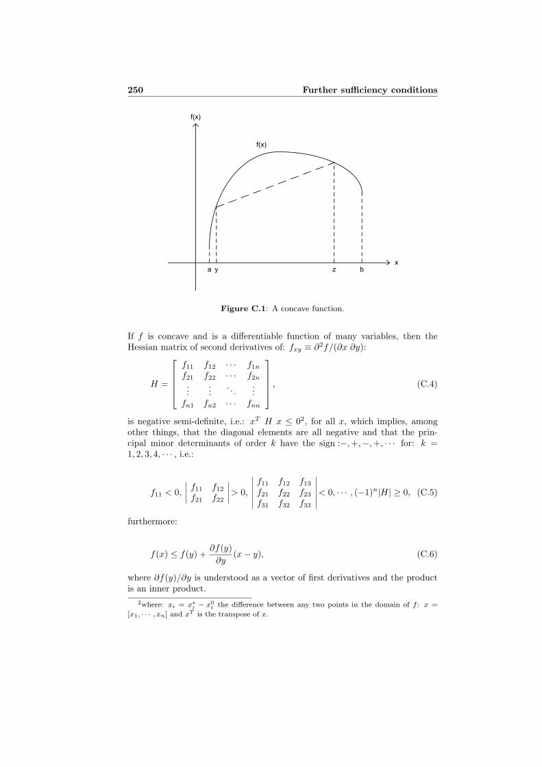
250 Further sufficiency conditions
a by z
f(x)
x
f(x)
Figure C.1: A concave function.
If f is concave and is a differentiable function of many variables, then theHessian matrix of second derivatives of: fxy ≡ ∂2f/(∂x ∂y):
H =
f11 f12 · · · f1n
f21 f22 · · · f2n
......
. . ....
fn1 fn2 · · · fnn
, (C.4)
is negative semi-definite, i.e.: xT H x ≤ 02, for all x, which implies, amongother things, that the diagonal elements are all negative and that the prin-cipal minor determinants of order k have the sign :−,+,−, +, · · · for: k =1, 2, 3, 4, · · · , i.e.:
f11 < 0,f11 f12
f21 f22> 0,
f11 f12 f13
f21 f22 f23
f31 f32 f33
< 0, · · · , (−1)n|H| ≥ 0, (C.5)
furthermore:
f(x) ≤ f(y) +∂f(y)
∂y(x− y), (C.6)
where ∂f(y)/∂y is understood as a vector of first derivatives and the productis an inner product.
2where: xi = x∗i − x0i the difference between any two points in the domain of f : x =
[x1, · · · , xn] and xT is the transpose of x.

C.1 Concave and convex functions 251
For a convex, differentiable function of several variables the Hessian matrixshould be positive semi-definite, equally implying that: xT H x ≥ 0, for all xand:
f(x) ≥ f(y) +∂f(y)
∂y(x− y). (C.7)
Most textbooks on dynamic optimisation and optimal control discuss convexityand concavity of functions in depth. The reader is, for example, referred toKamien and Schwartz (1993, Appendix A, Section 3).


Appendix D
Partial derivatives
D.1 For optimal control problem A4/B3/C1
The partial derivative expressions in equations 5.121 to 5.129 are as follows,using the product rule:
d(f(x)g(x)
)
dx=
df(x)dx
g(x) + f(x)dg(x)dx
, (D.1)
that is:
∂Vk(t)∂Vl(t)
=∑
i∈I
∑
j∈J i
∑
m∈M
∑
r∈Rkij
θ1m
(Qi(t)
(∂Dij(t)∂Vl(t)
Gijmr(t) + Dij(t)∂Gijmr(t)
∂Vl(t)))
=∑
i∈I
∑
j∈J i
∑
m∈M
∑
r∈Rkij
θ1m
( Qi(t)Vl(t)
(Ω2ij(t)Gijmr(t) + Dij(t)Ω3ijmr(t)
)),
(D.2)
∂Vk(t)∂Vl(t)
=
1 if k = l;0 if k 6= l,
(D.3)
∂Vk(t)∂Cd
l (t)=−
∑
i∈I
∑
j∈J i
∑
m∈M
∑
r∈Rkij
θ1m
( Qi(t)Cd
l (t)
(Ω2ij(t)Gijmr(t)+
Dij(t)Ω3ijmr(t)))
,
(D.4)
∂Vk(t)∂Il(t)
=∑
i∈I
∑
j∈J i
∑
m∈M
∑
r∈Rkij
θ1m
( Qi(t)Il(t)
(β5Ω2ij(t)Gijmr(t)+
β5Dij(t)Ω3ijmr(t)))
,
(D.5)
253

254 Partial derivatives
∂Vk(t)∂Uv(t)
=∑
i∈I
∑
j∈J i
∑
m∈M
∑
r∈Rkij
θ1mQi(t)(Ω4ij(t)Gijmr(t)+Dij(t)Ω5ijmr(t)
),
(D.6)
∂Vk(t)∂Up
j (t)=
∑
i∈I
∑
j∈J i
∑
m∈M
∑
r∈Rkij
θ1mQi(t)(Ω7ij(t)Gijmr(t)+Dij(t)Ω8ijmr(t)
),
(D.7)
∂Rk(t)∂Vl(t)
=Ω9α4
∑
i∈I
∑
j∈J i
∑
m∈M
∑
r∈Rkij
θ1mΦ1m
( Qi(t)Vl(t)
(Ω2ij(t)Gijmr(t)+
Dij(t)Ω3ijmr(t)))
,
(D.8)
∂Rk(t)∂Cd
l (t)=− Ω9α4
∑
i∈I
∑
j∈J i
∑
m∈M
∑
r∈Rkij
θ1mΦ1m
( Qi(t)Cd
l (t)
(Ω2ij(t)Gijmr(t)+
Dij(t)Ω3ijmr(t)))
,
(D.9)
∂Rk(t)∂Il(t)
=Ω9α4
∑
i∈I
∑
j∈J i
∑
m∈M
∑
r∈Rkij
θ1mΦ1m
( Qi(t)Il(t)
(β5Ω2ij(t)Gijmr(t)+
β5Dij(t)Ω3ijmr(t)))
,
(D.10)
∂Rk(t)∂Uv(t)
=Ω9α4
∑
i∈I
∑
j∈J i
∑
m∈M
∑
r∈Rkij
θ1mΦ1mQi(t)(Ω4ij(t)Gijmr(t)+
Dij(t)Ω5ijmr(t)),
(D.11)
∂Rk(t)∂Up
j (t)=Ω9α4
∑
i∈I
∑
j∈J i
∑
m∈M
∑
r∈Rkij
θ1mΦ1mQi(t)(Ω7ij(t)Gijmr(t)+
Dij(t)Ω8ijmr(t)),
(D.12)
∂K(t)∂Vl(t)
=α4
∑
i∈I
∑
j∈J i
∑
m∈M
∑
r∈Rij
θ1mdr
( Qi(t)Vl(t)
(Ω2ij(t)Gijmr(t)+
Dij(t)Ω3ijmr(t)))
,
(D.13)

D.1 For optimal control problem A4/B3/C1 255
∂K(t)∂Cd
l (t)=− α4
∑
i∈I
∑
j∈J i
∑
m∈M
∑
r∈Rij
θ1mdr
( Qi(t)Cd
l (t)
(Ω2ij(t)Gijmr(t)+
Dij(t)Ω3ijmr(t)))
,
(D.14)
∂K(t)∂Il(t)
=α4
∑
i∈I
∑
j∈J i
∑
m∈M
∑
r∈Rij
θ1mdr
( Qi(t)Il(t)
(β5Ω2ij(t)Gijmr(t)+
β5Dij(t)Ω3ijmr(t)))
,
(D.15)
∂K(t)∂Uv(t)
=α4
∑
i∈I
∑
j∈J i
∑
m∈M
∑
r∈Rij
θ1mdrQi(t)(Ω4ij(t)Gijmr(t)+
Dij(t)Ω5ijmr(t)),
(D.16)
∂K(t)∂Up
j (t)=α4
∑
i∈I
∑
j∈J i
∑
m∈M
∑
r∈Rij
θ1mdrQi(t)(Ω7ij(t)Gijmr(t)+
Dij(t)Ω8ijmr(t)),
(D.17)
Using the triple product rule:
d(f(x)g(x)h(x)
)
dx=
df(x)dx
g(x)h(x)+f(x)dg(x)dx
h(x)+f(x)g(x)dh(x)
dx, (D.18)
that is:
∂P (t)∂Vl(t)
=α4
∑
i∈I
∑
j∈J i
∑
m∈M
∑
r∈Rij
( Qi(t)Vl(t)
(Ω2ij(t)Gijmr(t)Ω10r(t)+
Dij(t)Ω3ijmr(t)Ω10r(t) + Dij(t)Gijmr(t)Ω11r(t)Ω12ijmr(t)))
,
(D.19)
∂P (t)∂Cd
l (t)= −α4
∑
i∈I
∑
j∈J i
∑
m∈M
∑
r∈Rij
( Qi(t)Cd
l (t)
(Ω2ij(t)Gijmr(t)Ω10r(t)+
Dij(t)Ω3ijmr(t)Ω10r(t) + Dij(t)Gijmr(t)Ω11r(t)Ω12ijmr(t)))
,
(D.20)

256 Partial derivatives
∂P (t)∂Il(t)
=α4
∑
i∈I
∑
j∈J i
∑
m∈M
∑
r∈Rij
( Qi(t)Il(t)
(β5Ω2ij(t)Gijmr(t)Ω10r(t)+
β5Dij(t)Ω3ijmr(t)Ω10r(t) + Dij(t)Gijmr(t)Ω11r(t)Ω12ijmr(t)))
,
(D.21)
∂P (t)∂Uv(t)
=α4
∑
i∈I
∑
j∈J i
∑
m∈M
∑
r∈Rij
Qi(t)(Ω4ij(t)Gijmr(t)Ω10r(t)+
Dij(t)Ω5ijmr(t)Ω10r(t) + Dij(t)Gijmr(t)Ω11r(t)Ω12ijmr(t)),
(D.22)
∂P (t)∂Up
j (t)=α4
∑
i∈I
∑
j∈J i
∑
m∈M
∑
r∈Rij
Qi(t)(Ω7ij(t)Gijmr(t)Ω10r(t)+
Dij(t)Ω8ijmr(t)Ω10r(t) + Dij(t)Gijmr(t)Ω11r(t)Ω12ijmr(t)),
(D.23)
∂E(t)∂Vl(t)
=α4
∑
i∈I
∑
j∈J i
∑
m∈M
∑
r∈Rij
∑
lr∈r
θ1m
( Qi(t)Vl(t)
(Ω2ij(t)Gijmr(t)Ω13mr(t)+
Dij(t)Ω3ijmr(t)Ω13mr(t) + Dij(t)Gijmr(t)Ω14mr(t)))
,
(D.24)
∂E(t)∂Cd
l (t)=− α4
∑
i∈I
∑
j∈J i
∑
m∈M
∑
r∈Rij
∑
lr∈r
θ1m
( Qi(t)Cd
l (t)
(Ω2ij(t)Gijmr(t)Ω13mr(t)+
Dij(t)Ω3ijmr(t)Ω13mr(t) + Dij(t)Gijmr(t)Ω14mr(t)))
,
(D.25)
∂E(t)∂Il(t)
=α4
∑
i∈I
∑
j∈J i
∑
m∈M
∑
r∈Rij
∑
lr∈r
θ1m
( Qi(t)Il(t)
(β5Ω2ij(t)Gijmr(t)Ω13mr(t)+
β5Dij(t)Ω3ijmr(t)Ω13mr(t) + Dij(t)Gijmr(t)Ω14mr(t)))
,
(D.26)

D.1 For optimal control problem A4/B3/C1 257
∂E(t)∂Uv(t)
=α4
∑
i∈I
∑
j∈J i
∑
m∈M
∑
r∈Rij
∑
lr∈r
θ1mQi(t)(Ω4ij(t)Gijmr(t)Ω13mr(t)+
Dij(t)Ω5ijmr(t)Ω13mr(t) + Dij(t)Gijmr(t)Ω14mr(t)),
(D.27)
∂E(t)∂Up
j (t)=α4
∑
i∈I
∑
j∈J i
∑
m∈M
∑
r∈Rij
∑
lr∈r
θ1mQi(t)(Ω7ij(t)Gijmr(t)Ω13mr(t)+
Dij(t)Ω8ijmr(t)Ω13mr(t) + Dij(t)Gijmr(t)Ω14mr(t)),
(D.28)
∂Ml(t)∂Um
l (t)= β7α5
(Il(t)− Ip
)Um
l (t)β7−1, (D.29)
∂Uml (t)max
∂Vl(t)=
Uml (t)max
β7Ω11r(t)γ2
∂Rk(t)∂Vl(t)
, (D.30)
∂Uml (t)max
∂Cdl (t)
=Um
l (t)max
β7Ω11r(t)γ2
(∂Rk(t)∂Cd
l (t)+
α6(Il(t)− Ip)U cl (t)
Cdl
2(t)
), (D.31)
∂Uml (t)max
∂Il(t)=
Uml (t)max
β7Ω11r(t)(1 + γ2
(∂Rk(t)∂Il(t)
+ ξ1 − α6U c
l (t)Cd
l (t)
)− Ω11r(t)
α5(Il(t)− Ip)),
(D.32)
∂Uml (t)max
∂U cl (t)
= −Uml (t)max
β7Ω11r(t)γ2α6(Il(t)− Ip)
Cdl (t)
, (D.33)
Ω1ijmr(t) =
β3mβ1α1τ
0lr
( Vl(t)Ce
l (t)
)β1 if l ∈ r∈ Rij;0 if l /∈ r∈ Rij,
(D.34)
Ω2ij(t) =− b1λ2 exp(−λ2
(c∗ij(t)− c0
ij
))∑
m′∈M∑
r′∈Rijexp
(−λ3uijm′r′(t))
∑
m′∈M
∑
r′∈Rij
(exp (−λ3uijm′r′(t))Ω1ijm′r′(t)) ,(D.35)

258 Partial derivatives
Ω3ijmr(t) = λ1Gijmr(t) ∑j′∈J i
∑m′∈M
∑r′∈Rij
(Gij′m′r′(t) Ω1ij′m′r′(t)) if l /∈ r∈ Rij;∑j′∈J i
∑m′∈M
∑r′∈Rij
(Gij′m′r′(t) Ω1ij′m′r′(t))− Ω1ijmr(t) if l ∈ r∈ Rij,(D.36)
Ω4ij(t) =− b1λ2 exp(−λ2
(c∗ij(t)− c0
ij
))∑
m′∈M∑
r′∈Rijexp
(−λ3uijm′r′(t))
∑
m′∈M
∑
r′∈Rij
(exp (−λ3uijm′r′(t)) β4m′θ2m′fr′) ,(D.37)
Ω5ijmr(t) = λ1Gijmr(t) ∑j′∈J i
∑m′∈M
∑r′∈Rij
(Gij′m′r′(t) β4m′θ2m′fr′) if l /∈ r∈ Rij;∑j′∈J i
∑m′∈M
∑r′∈Rij
(Gij′m′r′(t) β4m′θ2m′fr′)− β4mθ2mdr if l ∈ r∈ Rij,(D.38)
Ω6ijmr(t) =
β4mθ2m if j = j′ in r′∈ Rij′;0 if j 6= j′ in r′∈ Rij′, (D.39)
Ω7ij(t) =− b1λ2 exp(−λ2c
∗ij(t)− c0
ij
))∑
m′∈M∑
r′∈Rijexp
(−λ3uijm′r′(t))
∑
m′∈M
∑
r′∈Rij
(exp (−λ3uijm′r′(t)) β4m′θ2m′) ,(D.40)
Ω8ijmr(t) = λ1Gijmr(t) ∑j′∈J i
∑m′∈M
∑r′∈Rij
(Gij′m′r′(t) Ω6ij′m′r′(t)) if l /∈ r∈ Rij;∑j′∈J i
∑m′∈M
∑r′∈Rij
(Gij′m′r′(t) Ω6ij′m′r′(t))− Ω6ijmr(t) if l ∈ r∈ Rij,(D.41)
Ω9 = w exp(vt)(1 + Sl)β6 , (D.42)
Ω10r(t) =dr
τr(t), (D.43)

D.2 For optimal control problem A3/B1/C2 259
Ω11r(t) =( −dr
τr(t)2
), (D.44)
Ω12ijmr(t) =
β1α1τ
0lr
(Vl(t)Ce
l (t)
)β1
if l ∈ r∈ Rij;0 if l /∈ r∈ Rij,
(D.45)
Ω13mr(t) = εm|p dlr
(dlr
τl(t)
)−β8m|p
, (D.46)
Ω14mr(t) =Ω13mr(t)Ω12ijmr(t)β8m|p
τl(t), (D.47)
D.2 For optimal control problem A3/B1/C2
Here, only the partial derivatives for the functional J (including smoothing andpenalty terms) of problem (A3/B1/C2) are given. The other derivatives canbe directly taken, or be easily derived, from the results in previous paragraph.
∂J(t)∂Vl(t)
=− β9
∑
i∈I
∑
j∈J i
((Qi(t)Xj(t)
) 12
exp(−β9c
∗ij(t)
)
∑
r∈Rij
(exp(−λ3uijmr)∑
r′∈Rijexp(−λ3uijmr′)
Ω1ijmr(t)Vl(t)
)),
(D.48)
∂J(t)∂Cd
l (t)=β9
∑
i∈I
∑
j∈J i
(Qi(t)Xj(t)
) 12
exp(−β9c
∗ij(t)
)
∑
r∈Rij
(exp(−λ3uijmr)∑
r′∈Rijexp(−λ3uijmr′)
Ω1ijmr(t)Cd
l (t)
)),
(D.49)
∂J(t)∂U c
l (t)= −2α71U
cl (t), (D.50)
∂J(t)
∂E(t)=
−2χ1(E(t)− E∗) if (E(t)− E∗) > 0;0 if (E(t)− E∗) ≤ 0.
(D.51)

260 Partial derivatives
D.3 For optimal control problem A4/B2/C3
Here, only the partial derivatives for the functional J (including smoothing andpenalty terms) of problem (A4/B2/C3) are given. The other derivatives canbe directly taken, or be easily derived, from the results in previous paragraph.
∂J(t)∂P (t)
= 1, (D.52)
∂J(t)∂U t
l (t)= −2α71U
tl (t), (D.53)
∂J(t)∂E(t)
= −2χ1(E(t)− E∗) if (E(t)− E∗) > 0;
0 if (E(t)− E∗) ≤ 0.(D.54)
D.4 For optimal control problem A4/B2/C4
Here, only the partial derivatives for the functional J (including smoothing andpenalty terms) of problem (A4/B2/C4) are given. The other derivatives canbe directly taken, or be easily derived, from the results in previous paragraph.
∂J(t)∂Vl(t)
=− 2∑
i∈I
∑
j∈J i
∑
k∈K
((Qi|k(t) c∗ij|k(t)− c∗ij(t0)
)Qi|k(t)
∑m′∈M
∑r′∈Rij
(exp
(−λ3uijm′r′|k(t))Ω1ijm′r′|k(t)
)∑
m′∈M∑
r′∈Rijexp
(−λ3uijm′r′|k(t))
),
(D.55)
∂J(t)∂Cd
l (t)=2
∑
i∈I
∑
j∈J i
∑
k∈K
((Qi|k(t) c∗ij|k(t)− c∗ij(t0)
)Qi|k(t)
∑m′∈M
∑r′∈Rij
(exp
(−λ3uijm′r′|k(t))Ω1ijm′r′|k(t)
)∑
m′∈M∑
r′∈Rijexp
(−λ3uijm′r′|k(t))
),
(D.56)
∂J(t)∂U t
l (t)= −2α71U
tl (t), (D.57)
∂J(t)∂E(t)
= −2χ1(E(t)− E∗) if (E(t)− E∗) > 0;
0 if (E(t)− E∗) ≤ 0.(D.58)

SamenvattingDutch summary
Duurzame ontwikkeling van stedelijk verkeer en ver-voer als dynamisch optimalisatieprobleem
Recente ontwikkelingen in stedelijk verkeer en vervoer dwingen beleidsmakersin toenemende mate bij de planning, het management en beheer en onderhoudvan verkeersinfrastructuur rekening te houden met een groot aantal complexeen soms onderling tegenstrijdige belangen zoals filebestrijding, emissiereductie,gebruik van schaarse hulpbronnen, gelijkheid en bereikbaarheid.
De huidige oplossing voor de verkeersproblemen zelf en de veranderende enzwaarder wordende eisen gesteld aan verkeers- en vervoerbeleid, wordt vaakgezocht in uitbreiding van de capaciteit van aanwezige infrastructuur, het betergebruiken van bestaande infrastructuur, het ontmoedigen danwel aanmoedigenvan het gebruik van bepaalde vervoerswijzen of pogingen verplaatsingspatronenvan mensen en goederen rechtstreeks te beınvloeden, conform het principe vanvoorspel-maak-beheers (predict-provide-manage). De beslissingen daaromtrentzijn meestal gebaseerd op ervaring (zogenaamde best-practices), bestaande the-orieen en methoden en technieken van vervoersplanning. Desondanks lijken hethuidige verkeers- en vervoersysteem en de gebruikte methoden, technieken enmodellen - zowel in ontwikkelde als in ontwikkelingslanden - niet noodzakelij-kerwijs te voldoen aan de eisen van duurzame ontwikkeling. Een duurzaamverkeers- en vervoersysteem kan alleen worden bereikt wanneer gebruik wordtgemaakt van een nieuw paradigma voor duurzaam verkeer en vervoer in com-binatie met een daarbij horend raamwerk voor analyse en ontwerp.
In dit proefschrift wordt een theoretisch kader in combinatie met een metho-dologie geschetst, waarin voorwaarden van duurzame ontwikkeling rechtstreekszijn geıntegreerd in modellen voor verkeersbeleid en vervoersplanning, in bij-zonder de vervoersvraagmodellen. Met de opgedane kennis en de uitkomstenvan dit onderzoek zal het mogelijk zijn efficienter en effectiever gebruik te ma-ken van beschikbare en betaalbare schaarse hulpbronnen in het belang van deontwikkeling van het verkeers- en vervoersysteem zelf.
Met het paradigma van duurzaam verkeer en vervoer wordt een verkeers- en
261

262 Samenvatting (Dutch summary)
vervoersysteem aangeduid binnen randvoorwaarden van milieu, energie, ver-keersveiligheid en beschikbare budgetten. Dit paradigma is gebaseerd op demondiale boodschap van wetenschappers en politici dat ongebreidelde groeiop onze planeet zal leiden tot overmatig en onomkeerbaar gebruik van milieu-kundige en ecologische bronnen en uiteindelijk zelfs tot onze mogelijke onder-gang. Het paradigma van een duurzame transportontwikkeling sluit hierbij aanen probeert een veelomvattend beslissingsondersteunend systeem te promoten,waarin ontwikkelingen in verkeer en vervoer in termen van mobiliteit, bereik-baarheid en verplaatsingen zich afspelen binnen de eerder genoemde randvoor-waarden van milieu, energie en beschikbare budgetten. Het systeem anticipeertderhalve op beheerst gebruik van schaarse bronnen, terwijl het zich (gestuurd)ontwikkelt in termen van kwaliteit en kwantiteit van doorstroming.
De afgelopen decennia zijn vervoersvraagmodellen ter ondersteuning van hetcomplexe proces van vervoersplanning geevolueerd van een simpele heuristiektot een geavanceerd sequentieel vierstaps-verkeersmodel met deelmodellen voorritgeneratie, ritdistributie, vervoerswijzekeuze en toedeling. Dit geavanceerdemodel is desondanks nog regelmatig bron van kritiek, met name in relatie tothet thema duurzame ontwikkeling en verkeer en vervoer. Zo is er kritiek ophet sequentiele en statische karakter van het vierstaps-verkeersmodel, waardoornauwelijks sprake kan zijn van een (simultane) terugkoppeling naar beslissin-gen in voorgaande stappen van dit model. Daarnaast bestaat er kritiek tenaanzien van de inelasticiteit van het ritgeneratie deelmodel voor veranderingenin bereikbaarheid, waardoor het verkeersmodel ongevoelig is voor - de alge-meen aangenomen - aanzuigende werking van nieuwe infrastructuur. Ook heteerder genoemde typische gebruik van het verkeersmodel conform het princi-pe van voorspel-maak-beheers, een vraagvolgende benadering, stuit vaak opkritiek. Limieten aan schaarse bronnen vereisen immers een aanbodgestuurdebenadering conform het principe van maak-beheers-voorspel. Een verkeersmo-del moet derhalve al redenerende vanuit een expliciet verkeersbeleidsdoel enkennis over beschikbare schaarse bronnen, komen tot een set aan verkeer- envervoer gerelateerde maatregelen.
Naast deze punten van kritiek, kan ook worden gesteld dat het traditionele ver-keersmodel minder bruikbaar is voor beleidsmakers als dit model geen rekeninghoudt met de continue verandering in het verplaatsingsgedrag van de gebruikerszelf (de reizigers), de prestatie van het verkeers- en vervoersysteem (in termenvan kwaliteit en kwantiteit van doorstroming) en de complexe en onderlingafhankelijke doelen van betrokken beleidsmakers. Het zijn namelijk niet de in-dividuele wensen en beslissingen van de betrokken gebruikers en beleidsmakersdie bepalend moeten zijn voor de te nemen maatregelen, maar de onderlingsamenhangende toestanden van hun individuele systemen. Dynamische opti-malisatie is bij uitstek geschikt om tegemoet te komen aan bovengenoemdekritiek. Hierbij worden tegelijkertijd de volgorde en het tijdstip van te nemenverkeersgerelateerde maatregelen bepaald, om zo een vooraf geexpliciteerd ver-keersbeleidsdoel te kunnen verwezenlijken op een vooraf vastgestelde termijn.

263
Dit lijkt dan ook een logische vervolgstap in de ontwikkeling van verkeersmo-dellen.
In dit onderzoek is een dergelijk verkeersmodel ontwikkeld, besproken en geım-plementeerd, gebaseerd op een conceptualisatie en karakterisering van duurza-me transportontwikkeling als optimalisatieprobleem. De bouwstenen van hettraditionele vierstaps-verkeersmodel worden zeer bruikbaar verondersteld voorde vraagstelling in dit onderzoek en worden dus ook als zodanig gebruikt bijhet opstellen van het dynamische model. Een proactieve benadering van ver-keersproblemen conform het principe van maak-beheers-voorspel (‘voorkom’),in tegenstelling tot dat van voorspel-maak-beheers, is het resultaat, waardooreen wezenlijke bijdrage geleverd kan worden in het complexe (politieke) be-sluitvormingsproces rondom duurzaam verkeer en vervoer.
Het dynamische model maakt gebruik van een relaxatieformulering, waarinde toestandsvariabelen zich geleidelijk aanpassen aan het gewenste evenwicht,afhankelijk van de snelheid van aanpassing, die kan verschillen per type toe-standsvariabele. In het transportmodel wordt een aantal standaard toestands-variabelen, - zoals verkeersvraag (per link in het netwerk), infrastructuuraan-bod (en daarmee de effectieve capaciteit), het aantal gereden kilometers inhet netwerk, de reizigersdoorstroming door het netwerk en de totale emissievan schadelijke stoffen in het netwerk - gemodelleerd middels gewone diffe-rentiaalvergelijkingen. De verkeersvraag wordt bepaald vanuit sociaalecono-mische variabelen in de zones van het studiegebied, gebruikmakend van eendiscrete-keuze model, analoog aan het zwaartekrachtmodel, en is in omvangmede afhankelijk van de verkeersprestatie in het netwerk. De kwaliteit vanhet wegdek van een link, en daarmee de effectieve capaciteit, neemt auto-noom af, danwel door slijtage ten gevolge van aslasten van het verkeer. Deevenwichtswerking tussen verkeersvraag en infrastructuuraanbod wordt conti-nu verstoord door bestemmings-, vervoerswijze- en routekeuzegedrag van rei-zigers, maar ook door de aanzuigende werking van verkeersinfrastructuur. Devervoersplanner staan verschillende beslissingsvariabelen ter beschikking, diedit evenwicht proberen te beınvloeden of te sturen. Hij kan zo aanbodzij-degerelateerde beslissingsvariabelen zoals capaciteitsuitbreiding of onderhoud,maar ook vraagzijdegerelateerde beslissingsvariabelen als beprijzing inzetten.Gestuurd door een gekwantificeerd verkeersbeleidsdoel - zoals congestiemini-malisatie, bereikbaarheidsmaximalisatie, reizigersdoorstromingsmaximalisatieof gelijkheidsmaximalisatie - maar ook door beperkingen opgelegd aan de waar-de van de beslissingsvariabele of die van een toestandsvariabele - zoals totaleemissies - wordt nu de regelstrategie (in termen van volgorde en het momentvan inzetten van de beslissingsvariabelen) bepaald.
Het nieuwe verkeersmodel kan in zijn huidige vorm direct worden gebruiktvoor de modellering van strategische netwerken met een beperkt aantal (geag-gregeerde) zones en (geaggregeerde) links. Uitgewerkt als randwaardeprobleemin continue-tijd met het Pontryagin Maximum Principe, produceert het modelregelstrategieen om een duurzaam en ontwikkeld verkeers- en vervoersysteem te

264 Samenvatting (Dutch summary)
bereiken, waarbij tegelijkertijd allerlei informatie over de toestandsvariabelenen de bijbehorende schaduwprijzen (de zogenaamde costates) wordt gegene-reerd. Het dynamische model is desondanks nog niet volledig geımplementeerdmet een ‘complete’ dataset, waardoor thans geen algemeen geldende beleids-conclusies kunnen worden getrokken. De belangrijkste reden hiervoor is de ge-bleken tekortkoming in robuustheid van de gekozen optimalisatiemethode, metname in relatie tot de interactie van beslissingsvariabelen en bij niet-lineairebeslissingsvariabelen. Desondanks kan zowel uit deze eerste ontwikkelingsstapvan het complexe model, als op grond van de diverse cases opgemaakt wor-den dat het haalbaar zal zijn een volledig bruikbaar model te implementeren,parameters te schatten en het model toe te passen in een strategische vervoers-planningsstudie.

Bibliography
Akinyemi, E. O. (1997). A total performance approach to traffic managementfor sustainable development of communities in third-world cities, ResourcePapers for the 1997 ITE International Conference, Tampa, USA, pp. 191–209.
Akinyemi, E. O. (1998). Engineering and urban mobility enhancement in de-veloping countries, CODATU VIII Conference, Cape Town, South Africa,pp. 715–719.
Akinyemi, E. O. and Zuidgeest, M. H. P. (2000). Sustainable development &transportation: past experiences and future challenges, World TransportPolicy and Practice 6(1): 31–39.
Akinyemi, E. O. and Zuidgeest, M. H. P. (2002). Managing transportationinfrastructure for sustainable development, Computer-Aided Civil and In-frastructure Engineering 17(3): 148–161.
Al-Azzawi, M. (2001). Developing a ‘rapid’ strategic land-use and transportpolicy model using EMME/2, 10th European EMME/2 Users Group Con-ference, Thessaloniki, Greece.
Al-Deek, H., Wayson, R. and Radwan, A. (1995). Methodology for evalua-ting ATIS impacts on air quality, Journal of Transportation EngineeringJuly/August 1995: 376–384.
Anderson, J. E. (2003). Public Policymaking, fifth edn, Houghton Mifflin Com-pany, Boston, USA.
Andersson, J. (2001). Multiobjective Optimization in Engineering Design: Ap-plications to Fluid Power Systems, PhD thesis, Linkoping Studies in Scien-ce and Technology No. 675, University of Linkoping, Linkoping, Sweden.
Asian Development Bank (2003). Appendix on adverse health and environmen-tal effects from vehicle emissions, Policy Guidelines for Reducing VehicleEmissions in Asia, Asian Development Bank, Manila, The Philippines.
Banister, D. (2002). Transport Planning, Transport, Development and Sustai-nability, second edn, Sponn Press, London, England.
265

266 BIBLIOGRAPHY
Banister, D. and Berechman, J. (2000). Transport Investment and EconomicDevelopment, UCL Press, London, England.
Barkenbus, J. (1998). Expertise and the policy cycle, Report NCEDR/99-04, University of Tennessee: Energy, Environment, and Resources Center(NCEDR), Knoxville, USA.
Barten, H. (2004). Optimalisatie in de Vervoersplanning, Master’s thesis, Uni-versity of Twente, Enschede, The Netherlands. [In Dutch].
Bates, J. (2001). History of demand modelling, in D. A. Hensher and K. J.Button (eds), Handbook of Transport Modelling, Vol. 1 of Handbooks inTransport, Pergamon, Amsterdam, The Netherlands, chapter 2, pp. 11–33.
Becker, E., Jahn, T., Stiess, I. and Wehling, P. (1997). Sustainability: Across-disciplinary concept for social transformations, MOST Policy Pa-pers 6, United Nations Educational, Scientific and Cultural Organization(UNESCO), Paris, France.
Bell, M. G. H. and Allsop, R. E. (1998). Introduction, in M. G. H. Bell (ed.),Transportation Networks: Recent Methodological Advances, Selected pro-ceedings of the 4th Euro transportation meeting, Elsevier Science & Tech-nology, Oxford, England.
Bell, M. G. H. and Iida, Y. (1999). Transportation Network Analysis, JohnWiley & Sons, Chichester, England.
Ben-Akiva, M. and Lerman, S. R. (1985). Discrete Choice Analysis: Theoryand Applications to Travel Demand, The MIT Press, Cambridge, Massa-chusetts, USA.
Bertrand, R. and Epenoy, R. (2002). New smoothing techniques for solvingbang-bang optimal control problems - numerical results and statisticalinterpretation, Optimal Control Applications and Methods 23: 171–197.
Bierman, M. O. (2004). Induced Travel: Relating Accessibility and Trip Fre-quency, Master’s thesis, University of Twente, Enschede, The Netherlands.
Bluemel, H. (1999). The berlin urban traffic master plan: new approaches to theintegration of transport, land use and environmental planning, Clean AirInitiative in Latin American Cities. Clean Air Workshop for the MexicoCity Metropolitan Area, Mexico City, Mexico.
Bovy, P. H. L. and Van der Zijpp, N. J. (1999). Transportation modelling,Lecture Note CTvk4800, Delft University of Technology, Delft, The Ne-therlands.
Bryson, A. E. and Ho, Y. (1975). Applied Optimal Control: Optimization,Estimation and Control, Taylor & Francis, USA.

BIBLIOGRAPHY 267
BTE (1996). Roads, vehicle performance and greenhouse: costs and emissionbenefits of smoother highways, Working Paper 32, Bureau of Transportand Communications Economics, Australia.
BTE (1998). Urban transport models: A review, Working Paper 39, Bureauof Transport and Communications Economics, Australia.
Bureau of Public Roads (1964). Traffic Assignment Manual, Department ofCommerce, Urban Planning Division, Washington D.C., USA.
Buttler, H. and Shortreed, J. H. (1978). Investment planning of a road link,Transportation Research 12: 357–366.
Camagni, R. (1998). Sustainable urban development: definition and reasons fora research programme, International Journal on Environment and Pollu-tion 10(1): 6–27.
Camagni, R., Capello, R. and Nijkamp, P. (1998). Towards sustainable citypolicy: an economy-environment technology nexus, Ecological Economics24: 103–118.
Cervero, R. (2002). Induced travel demand: research design, empirical eviden-ce, and normative policies, Journal of Planning Literature 17(1): 3–20.
Chiou, S. W. (1999). Optimization of area traffic control for equilibrium net-work flows, Transportation Science 33(3): 279–289.
Colucci-Rios, B. and Sinha, K. (1985). Optimal pavement management ap-proach using roughness measurements, Transportation Research Record1048: 14–22.
Constantin, I. and Florian, M. (1995). Optimizing frequencies in a transit net-work: a nonlinear bi-level programming approach, Transactions in Ope-rational Research 2(2): 149–164.
Crozet, Y. and Marlot, G. (2001). Congestion and road pricing: where is the“bug”?, Proceedings of the 9th World Conference on Transport Research,Seoul, South Korea.
CST (1997). Definition and vision of sustainable transportation, Technical re-port, The Centre for Sustainable Transportation (CST), Toronto, Canada.
Dadebo, S. A., McAuley, K. B. and McLellan, P. J. (1998). On the computationof optimal singular and bang-bang controls, Optimal Control Applicationsand Methods 19: 287–297.
Dahlgren, J. (2003). The benefits of accommodating latent demand, Trans-portation Research Board (TRB) 2003 Annual Meeting CD-ROM, Was-hington D.C., USA.
Daly, H. E. (1991). Steady-State Economics, second edn, Island Press, Was-hington D.C., USA.

268 BIBLIOGRAPHY
De Borger, B. and Wouters, S. (1998). Transport externalities and optimalpricing and supply decisions in urban transportation, Regional Scienceand Urban Economics 28(2): 163–197.
De Cea, J. and Fernandez, E. (2001). Transit-assignment models, in D. A. Hens-her and K. J. Button (eds), Handbook of Transport Modelling, Vol. 1 ofHandbooks in Transport, Pergamon, Amsterdam, The Netherlands, chap-ter 30.
De la Barra, T. (1989). Integrated Land Use and Transport: Decision Chainsand Hierarchies, Cambridge University Press, Cambridge, New York,USA.
De la Barra, T. (n.d.). Improved logit formulations for integrated land use,transport and environmental models, Modelistica Systems and Planning .*http://www.modelistica.com/papers/suecia/suecia.htm
DETR (2002). Social exclusion and the provision and availability of publictransport, Technical report, Department of the Environment, Transportand the Regions (DETR), London, England.
Donaghy, K. P. and Schintler, L. A. (1994). Optimal policies for reducing con-gestion of major commuting arteries in a growing urbanized area, Journalof Planning and Research 13: 189–198.
Donaghy, K. P. and Schintler, L. A. (1998). Managing congestion, polluti-on, and pavement conditions in a dynamic transportation network model,Transportation Research 3D(2): 59–80.
ECMT (1995). Urban Travel and Sustainable Development, European Confe-rence of Ministers of Transport (ECMT), Paris, France.
English dictionary (2000). The American Heritage Dictionary of the EnglishLanguage, Houghton Mifflin Publishers, Massachusetts, USA.
ESCAP-AITD (2001). Sustainable transport pricing and charges: Principlesand issues, Technical report, United Nations - Economic and Social Com-mission for Asia and the Pacific (UN-ESCAP), Asian Institute of Trans-port Development (AITD), Bangkok, Thailand.
European Commission (1998). OPTIMA: Optimisation of Policies for Trans-port Integration in Metropolitan Areas, Office for Official Publications ofthe European Communities, Luxembourg.
European Commission (2000). EU transport in figures, Technical report, Euro-pean Commission Directorate-General for Energy and Transport, Brussels.
Eurostat (2001). Panorama of transport: Statistical overview of road, rail,inland waterways and air transport in the european union (data 1970 -1999), Technical report, Eurostat, European Union (EU), Luxembourg.

BIBLIOGRAPHY 269
Ferrari, P. (1995). Road pricing and network equilibrium, Transportation Re-search 29B(5): 357–372.
Ferrari, P. (1999). A model of urban transport management, TransportationResearch 33B(1): 43–61.
Friesz, T. L. (1985). Transportation network equilibrium, design and aggregati-on: key developments and research opportunities, Transportation Research19A(5/6): 413–427.
Friesz, T. L. and Bernstein, D. (2001). Analytical dynamic traffic assignmentmodels, in D. A. Hensher and K. J. Button (eds), Handbook of TransportModelling, Vol. 1 of Handbooks in Transport, Pergamon, Amsterdam, TheNetherlands, chapter 11, pp. 181–195.
Friesz, T. L. and Fernandez, J. E. (1979). A model of optimal trans-port maintenance with demand responsiveness, Transportation Research13B(4): 317–339.
Friesz, T. L. and Shah, S. (1998). Foundations of a theory of disequilibriumnetwork design, in M. G. H. Bell (ed.), Transportation Networks: RecentMethodological Advances, Selected Proceedings of the 4th Euro Trans-portation Meeting, Elsevier Science & Technology, Oxford, England.
Gandolfo, G. (1993). Continuous-time econometrics has come of age, in G. Gan-dolfo (ed.), Continuous Time Econometrics: Theory and Applications,Chapman & Hall, London, England, chapter 1, pp. 1–11.
Gandolfo, G. (1997). Economic Dynamics, Springer, Berlin, Germany.
Gauthier, H. (1970). Geography, transportation and regional development,Economic Geography 46: 612–619.
Geurs, K. T. and Ritsema van Eck, J. R. (2001). Accessibility measures: Reviewand applications, Report RIVM 408505 006, RIVM National Institute ofPublic Health and the Environment, Bilthoven, The Netherlands.
Goodwin, P. B. (1992). A review of new demand elasticities with special refe-rence to short and long run effects of price changes, Journal of TransportEconomics and Policy 26(2): 155–169.
Goodwin, P. B. (1996). Empirical evidence on induced traffic, Transportation23: 35–54.
Goodwin, P. B. (1999). Transformation of transport policy in Great Britain,Transportation Research 33A(7-8): 655–669.
Goodwin, P., Kitamura, R. and Meurs, H. (1990). Some principles of dynamicanalysis of travel behaviour, in P. Jones (ed.), Developments in Dynamicand Activity-based Approaches to Travel Analysis, Aldershot, Avebury,England, pp. 56–73.

270 BIBLIOGRAPHY
Goudappel Coffeng (2003). PROMILspatial, Computer program, GoudappelCoffeng consultants, Deventer, The Netherlands.
Gudmundsson, H. (2001). Indicators for performance measures for transporta-tion, environment and sustainability in North America, German MarshallFund Fellowship report 148, National Environmental Research Institute,Roskilde, Denmark.
Gudmundsson, H. (2003). Concepts of sustainable transport: making sense ornot?, PhD course: Sustainable Transport Futures, Roskilde, Denmark.
Gudmundsson, H. and Hojer, M. (1996). Sustainable development principlesand their implications for transport, Ecological Economics 19: 269–282.
Haas, R. C. G. and Hudson, W. R. (1978). Pavement Management Systems,Krieger Publishing Company, Florida, USA.
Hansen, W. G. (1959). How accessibility shapes land use, Journal of AmericanInstitute of Planners 25(2): 72–76.
Hau, T. D. (1992). Economic fundamentals of road pricing: A diagrammaticanalysis, World Bank Policy Research Working Paper Series WPS 1070,The World Bank, Washington D.C., USA.
Hilling, D. (1996). Transport and Developing Countries, Routledge, London,England.
Hillman, M. and Adams, J. (1992). Safer driving - safer for whom?, Conferenceon Eurosafe: Safer Driving in Europe, The association of London Boroughroad safety officers, London, England.
Hinloopen, E., Nijkamp, P. and Rietveld, P. (1983). The regime method: a newmulti-criteria technique, in P. Hansen (ed.), Essays and Surveys on Multi-ple Criteria Decision Making, Springer Verlag, Berlin, Germany, pp. 146–155.
Hojer, M. (1998). Transport telematics in urban systems: a backcasting Delphistudy, Transportation Research 3D(6): 445–463.
Hojer, M. and Mattsson, L. (2000). Determinism and backcasting in futurestudies, Futures 32: 613–634.
Huapu, L. and Peng, Z. (2001). A study on urban transport planning modelintegrating land-use mode and environment capacity based on sustaina-ble development, Proceedings of the 9th World Conference on TransportResearch, Seoul, South Korea.
ICLEI (1996). The Local Agenda 21 Planning Guide: An Introduction to Sustai-nable Development Planning, International Council on Local EnvironmentInitiatives (ICLEI), Toronto, Canada.

BIBLIOGRAPHY 271
Immers, L. H. and Oosterbaan, C. G. J. (1991). A model for the calculationof environment-friendly traffic flows in urban networks, Proceedings of the70th Annual TRB Meeting, Washington D.C., USA.
Intriligator, M. D. and Sheshinski, E. (1986). Toward a theory of planning,in W. P. Heller, R. M. Starr and D. A. Starett (eds), Social Choice andPublic Decision Making, Vol. 1 of Essays in Honour of Kenneth J. Arrow,Cambridge University Press, England, chapter II-7.
Jansen, G. R. M. and Bovy, P. H. L. (1982). The effects of zone size andnetwork detail on all-or-nothing and equilibrium assignment outcomes,Traffic Engineering and Control 23(6): 311–317.
Jayakrishnan, R., Tsai, W. K. and Chen, A. (1995). A dynamic traffic as-signment model with traffic flow relationships, Transportation Research3C(1): 51–72.
Kamien, M. I. and Schwartz, N. L. (1993). Dynamic Optimization: The Cal-culus of Variations and Optimal Control in Economics and Management,North-Holland, New York, USA.
Kay, S. M. (1993). Fundamentals of Statistical Signal Processing: EstimationTheory, Vol. 1, Prentice Hall PTR, New Jersey, USA.
Kierzenka, J. and Shampine, L. F. (2001). A BVP solver based on residual con-trol and the Matlab PSE, ACM Transactions on Mathematical Software27(3): 299–316.
Kim, K. (1998). A Transportation Planning Model for State Highway Mana-gement: A Decision Support System Methodology to Achieve SustainableDevelopment, PhD thesis, Virginia Polytechnic Institute and State Uni-versity, Virginia, USA.
Kim, T. J. and Hoskote, N. G. (1983). Estimating mobile source pollutantemission: methodological comparison and planning implications, Envi-ronmental Monitoring and Assessment 3: 1 – 12.
Knoflacher, H., Pfaffenbichler, P. C. and Emberger, G. (2000). A strategictransport model-based tool to support urban decision making processes,in J. C. Mangin and M. Miramond (eds), 2nd International Conferenceon Decision Making in Urban and Civil Engineering, Lyon, France.
Lasswell, H. D. (1951). The policy orientation, in D. Lerner and H. D. Lasswell(eds), The Policy Sciences, Stanford University Press, Paolo Alto, USA.
Lee, D. B. (1994). Retrospective on large-scale urban models, Journal of theAmerican Planning Association Winter 1994(1): 35–40.
Lensink, S. M. (2002). Applying optimal control to minimize energy use dueto road infrastructure expansion, Interim Report IR-02-071, InternationalInstitute for Applied Systems Analysis (IIASA), Laxenburg, Austria.

272 BIBLIOGRAPHY
Leonard, D. and Van Long, N. (1992). Optimal Control Theory and StaticOptimization in Economics, Cambridge University Press, Cambridge, En-gland.
Lindquist, E. (1998). Moving towards sustainability: transforming a compre-hensive land use and transportation plan, Transportation Research Record1617: 1–9.
Litman, T. A. (n.d.a). Reinventing transportation: Exploring the paradigmshift needed to reconcile transportation and sustainability objectives, Vic-toria Transport Policy Institute . *http://www.vtpi.org/
Litman, T. A. (n.d.b). Sustainable transportation indicators, Victoria Trans-port Policy Institute . *http://www.vtpi.org/
Litman, T. A. and Burwell, D. (n.d.). Issues in sustainable transportation,Victoria Transport Policy Institute . *http://www.vtpi.org/
Malone, K. M. (2001). The Scenario Explorer for passenger transport: a stra-tegic model for long term travel demand forecasting, Technical report,TNO-INRO, Delft, The Netherlands.
Manheim, M. L. (1979). Fundamentals of Transportation System Analysis,MIT Press, Cambridge, Massachuchets.
Martinez-Alier, J. (n.d.). Ecological - economics, International encyclopedia ofthe social and behavioral sciences, Elsevier Science & Technology. article4.9, number 9. *http://www.iesbs.com/
May, A. D., Matthews, B. and Jarvi-Nykanen, T. (2001). Decision makingrequirements for the formulation of sustainable urban land use - trans-port strategies, Proceedings of the 9th World Conference on TransportResearch, Seoul, South Korea.
Meadows, D. H., Meadows, D. L. and Randers, J. (1992). Beyond the Limits:Confronting Global Collapse, Envisioning a Sustainable Future, Earthscanpublications, London, England.
Meadows, D. H., Meadows, D. L., Randers, J. and Behrens, W. W. (1972).The Limits to Growth, Universe books, New York, USA.
Meng, Q. and Yang, M. (2002). Benefit distribution and equity in road networkdesign, Transportation Research 36B: 19–35.
Meyer, M. D. and Miller, E. J. (2001). Urban Transportation Planning, McGraw Hill, New York, USA.
Miller, J. S. and Demetsky, M. J. (1999). Reversing direction of transportati-on planning process, Journal of Transportation Engineering May/June1999: 231–237.

BIBLIOGRAPHY 273
Ministerie van de Vlaamse Gemeenschap (2001). Naar een duurzame mobili-teit in Vlaanderen, Mobiliteitsplan Vlaanderen, Departement Leefmilieuen Infrastructuur, Brussels, Flanders, Belgium. [In Dutch].
Morgan, M. G. and Henrion, M. (1990). Uncertainty: A Guide to Dealingwith Uncertainty in Quantitative Risk and Policy Analysis, CambridgeUniversity Press, Cambridge, England.
Morris, J. M., Dumble, P. L. and Wigan, M. R. (1979). Accessibility indicatorsfor transport planning, Transportation Research 13A: 91–109.
Nagurney, A. (2000). Sustainable Transportation Networks, Edward Elgar Pu-blishing, Inc., USA.
Naidu, D. S. (2003). Optimal Control Systems, CRC Press, Florida, USA.
NCHRP (1997). Quantifying congestion, NCHRP report 398, National Coo-perative Highway Research Program (NCHRP), NAP, Washington D.C.,USA.
Newman, P. and Kenworthy, J. (1999). Sustainability and Cities: OvercomingAutomobile Dependence, Island Press, Washington D.C., USA.
Nijkamp, P. and Opschoor, H. (1995). Urban environmental sustainability:critical issues and policy measures in a third world context, in Chatterjee(ed.), Urban Policies in Third World Countries, MacMillan, New York,USA.
Nijkamp, P. and Reggiani, A. (1988). Analysis of dynamic spatial interactionmodels by means of optimal control, Geographical Analysis 20(1): 18–30.
NIST-SEMATECH (n.d.). e-Handbook of Statistical Methods, National Institu-te of Standards and Technology - SEmiconductor MAnufacturing TECH-nology, USA. *http://www.itl.nist.gov/div898/handbook/
Noland, R. B. (2001). Relationships between highway capacity and inducedvehicle travel, Transportation Research 35A: 47–72.
Noland, R. B. and Lem, L. L. (2002). A review of the evidence for inducedtravel and changes in transportation and environmental policy in the USand the UK, Transportation Research 7D: 1–26.
Odoki, J. B., Kerali, H. R. and Santorini, F. (2001). An integrated model forquantifying accessibility-benefits in developing countries, TransportationResearch 35A: 601–623.
Oppenheim, N. (1995). Urban Travel Demand Modeling: From Individual Choi-ces to General Equilibrium, John Wiley & Sons, New-York, USA.
Ortuzar, J., Martınez, F. J. and Varela, F. J. (2000). Stated preference model-ling accessibility, International Planning Studies 5: 65–85.

274 BIBLIOGRAPHY
Ortuzar, J. and Willumsen, L. G. (2001). Modelling Transport, third edn, JohnWiley & Sons, Chicester, England.
Oude Moleman, T. (2001). Sustainable Performance - Measuring Sustainabi-lity of an Urban Transport System, Master’s thesis, University of Twente,Enschede, The Netherlands.
Owen, W. (1987). Transportation and World Development, Hutchinson, Lon-don, England.
Paterson, W. D. O. (1987). Road Deterioration and Maintenance Effects: Mo-dels for Planning and Management, The Johns Hopkins University Press,Baltimore, USA.
Pearce, D. W. and Turner, R. K. (1990). Economics of Natural Resources andthe Environment, Harvester Wheatsheaf, London, England.
Peters, D. (2002). Life in times of the traffic jam: why smart cities are de-motorising, Sustainable Development International 2002(3): 157–161.
Pfaffenbichler, P. C. (2003). The Strategic, Dynamic and Integrated UrbanLand Use and Transport Model MARS (Metropolitan Activity RelocationSimulator), PhD thesis, University of Vienna, Austria.
Pfaffenbichler, P. C. and Shepherd, S. P. (2002). A dynamic model to appraisestrategic land-use and transport policies, European Journal of Transportand Infrastructure Research 2(3/4): 255–283.
Pigou, A. C. (1932). The Economics of Welfare, 4 edn, Macmillan and Co.,London, England.
Plaut, P. O. and Shmueli, D. F. (2000). Sustainable transport: a compara-tive analysis of Israel, the Netherlands and the United Kingdom, WorldTransport Policy and Practice 6(1): 40–58.
Pontryagin, L. S., Boltyanskii, V. G., Gamkrelidze, R. V. and Mischenko, E. F.(1962). The Mathematical Theory of Optimal Processes, John Wiley &Sons, New York, USA.
Prakash, A. B., D’A. Oliver, E. H. and Balcombe, K. (2001). Does building newroads really create extra traffic? Some new evidence, Applied Economics33: 1579–1585.
Press, W. H., Flannery, B. P., Teukolsky, S. A. and Vetterling, W. T. (eds)(1989). Numerical Recipes in Pascal: The Art of Scientific Computing,Cambridge University Press, Cambridge, England.
Replogle, M. (1991). Sustainability: a vital concept for transportation planningand development, Journal of Advanced Transportation 25(1): 3–18.
Roozenburg, N. F. M. and Eekels, J. (1998). Produktontwerpen, Structuur enMethoden, Malberg, Utrecht, The Netherlands. [In Dutch].

BIBLIOGRAPHY 275
SACTRA (1994). Trunk roads and the generation of traffic, Technical report,Department of transport, Standing Advisory Committee on Trunk RoadAssessment (SACTRA), London, England.
Sales Filho, L. H. (1998). The accessibility matrix: a new approach for evalu-ating urban transportation networks, Proceedings of the 8th World Con-ference on Transport Research (WCTR), Antwerp, Belgium.
Schwartz, A. L. (1996). Theory and Implementation of Numerical MethodsBased on Runge-Kutta Integration for Solving Optimal Control Problems,PhD thesis, University of California at Berkeley, USA.
Schwela, D. (2002). Air quality management, in GTZ (ed.), Sustainable trans-port: A sourcebook for policy-makers in developing cities, Vol. 5a, DeutscheGesellschaft fur Technische Zussammenarbeit (GTZ), Eschborn, Germany.
Schwela, D. and Zali, O. (eds) (1999). Urban Traffic Pollution, E&FN Spon,London, England.
Seierstad, A. and Sydsæter, K. (1987). Optimal Control Theory with EconomicApplications, Elsevier Science & Technology, Amsterdam, The Nether-lands.
Shampine, L. F., Kierzenka, J. and Reichelt, M. W. (2000). Solving boundaryvalue problems for ordinary differential equations in Matlab with bvp4c,Matlab documentation. *ftp://ftp.mathworks.com/pub/doc/papers/bvp/
Sheffi, Y. (1985). Urban Transportation Networks, Prentice-Hall, EnglewoodCliffs, USA.
Shresta, R. M., Anandarajah, G., Adhikari, S., Jiang, K. and Songli, Z. (2005).Energy and environmental implications of NOx emission reduction fromthe transport sector of Beijing: a least-cost planning analysis, Transporta-tion Research 10D: 1–11.
Stackelberg, H. V. (1934). Marktform und Gleichgewicht, Julius Springer, Vi-enna, Austria. [In German].
Steenbrink, P. A. (1974). Optimization of Transport Networks, John Wiley &Sons, London, England.
Tagore, M. R. and Sikdar, P. K. (1995). A new accessibility measure accountingmobility parameters, Selected Proceedings of the 7th World Conference onTransport Research (WCTR), Vol. 1, Sydney, Australia, pp. 305–315.
Talvitie, A. (1997). Things planners believe in, and things they deny, Trans-portation 24: 1–31.
Talvitie, A. (2001). Comment of Richard Willson’s paper: assessing communi-cative rationality as a transportation planning paradigm, Transportation28: 207–210.

276 BIBLIOGRAPHY
Tillema, F. (2004). Development of a Data Driven Land Use Transport Inter-action Model, PhD thesis, University of Twente, The Netherlands.
Tolley, R. S. and Turton, B. J. (1995). Transport Systems, Policy and Planning:A Geographical Approach, Longman, Harlow, England.
TRB (1997). Toward a sustainable future: adressing the long-term effects ofmotor vehicle transportation on climate and ecology, Special report 251,Transportation Research Board - National Research Council, WashingtonD.C., USA.
UNCED (1992). Agenda 21, Technical report, United Nations Conference onEnvironment & Development (UNCED), Rio de Janeiro, Brazil.
Van den Bergh, J. C. J. M. (1991). Dynamic Models for Sustainable Develop-ment, PhD thesis, Free University of Amsterdam, Amsterdam, The Ne-therlands.
Van den Boom, T. and De Schutter, B. (2004). Optimization in systems andcontrol, Lecture Note SC4090, Delft University of Technology, Delft, TheNetherlands.
Van Dieren, W. (ed.) (1995). Taking Nature into Account: A Report to TheClub of Rome, Springer Verlag, New York, USA.
Van Gent, A. L. (2005). Aggregating Transport Networks, Master’s thesis,University of Twente, Enschede, The Netherlands.
Van Nes, A. E. (2004). Environment Capacity in Dutch Urban Passenger Trans-port, Master’s thesis, University of Twente, Enschede, The Netherlands.
Van Wee, B. and Geurs, K. (2000). Backcasting as a tool to develop a sustaina-ble transport scenario assuming emission reductions of 80-90%, Innovation13(1): 47–62.
Vasconcellos, E. A. (2001). Urban Transport, Environment and Equity: TheCase for Developing Countries, Earthscan, London, England.
Vickerman, R. (2001). The concept of optimal transport systems, in K. J.Button and D. A. Hensher (eds), Handbook of Transport Systems andTraffic Control, Vol. 3 of Handbooks in Transport, Pergamon, Amsterdam,The Netherlands, chapter 5, pp. 47–59.
Von Weizsacker, E., Lovins, A. B. and Lovins, L. H. (1998). Factor Four:Doubling Wealth, Halving Resource Use, Earthscan, London, England.
Wachs, M. and Kumagai, T. G. (1973). Physical accessibility as a social indi-cator, Socio-Economic Planning Science 6: 357–379.
Wackernagel, M. and Rees, W. (1995). Our Ecological Footprint: ReducingHuman Impact on the Earth, New Society Publishers, Philadelphia, USA.

BIBLIOGRAPHY 277
WBCSD (2001). Mobility 2001, World Business Council for Sustainable Devel-opment, Geneva, Switzerland.
WCED (1987). Our Common Future, World Commission on Environment andDevelopment (WCED), Oxford, England.
White, N. P. and Senior, M. L. (1983). Transport Geography, Longman, Harlow,England.
Whitelegg, J. (1993). Transport for a Sustainable Future: The Case for Europe,John Wiley & Sons, Chichester, England.
Whitelegg, J. (2003). Car wars, The Guardian, March 26.
Williams, H. C. W. L. (1977). On the formation of travel demand models andeconomic evaluation measures of user benefit, Environment and PlanningA 9: 285–344.
Willson, R. (2001). Assessing communicative rationality as a transport plan-ning paradigm, Transportation 28: 1–31.
World Bank (1996). Sustainable Transport: Priorities for Policy Reform, TheWorld Bank, Washington D.C., USA.
World Bank (2002). Cities on the Move: A World Bank Urban TransportStrategy Review, The World Bank, Washington D.C., USA.
Wymer, C. R. (1992). Estimation of nonlinear continuous-time models from dis-crete data, in P. C. B. Phillips and V. B. Hall (eds), Models, Methods andApplications in Econometrics, Basil Blackwell, Oxford, England, pp. 91–114.
Wymer, C. R. (2001). Wysea: Systems Estimation and Analysis Programs,Software program, Dr. C.R. Wymer ([email protected]).
Yang, H. (1995). Heuristic algorithms for the bilevel origin-destination matrixestimation problem, Transportation Research 29B(4): 231 – 242.
Yang, H. and Bell, M. G. H. (1997). Traffic restraint, road pricing and networkequilibrium, Transportation Research 31B(4): 303–314.
Yang, H. and Bell, M. G. H. (1998). Models and algorithms for road net-work design: a review and some new developments, Transport Reviews18(3): 257 – 278.
Yang, H., Bell, M. G. H. and Meng, Q. (2000). Modeling the capacity andlevel of service of urban transportation networks, Transportation Research34B: 255 – 275.
Yang, H. and Huang, H. J. (1998). Principle of marginal-cost pricing: how doesit work in a general network?, Transportation Research 32A(1): 45–54.

278 BIBLIOGRAPHY
Zietsman, J. (2000). Incorporating Sustainability Performance Measures intothe Transportation Planning Process, PhD thesis, Texas A&M University,USA.
Zuidgeest, M. H. P., Akinyemi, E. O. and Van Maarseveen, M. F. A. M.(2001). Challenging sustainable accessibility: accessibility and mobilityconcepts in dynamic urban environments, CD-ROM 9th World Conferen-ce on Transport Research (WCTR), Seoul, Korea.
Zuidgeest, M. H. P. and Van Maarseveen, M. F. A. M. (2000). Transportationplanning for sustainable development, CD-ROM South-African TransportConference - Action in Transport for the new Millenium, CSIR ConferenceCentre, Pretoria, South Africa.
Zuidgeest, M. H. P., Witbreuk, M. J. G. and Van Maarseveen, M. F. A. M.(2000). Sustainable transport: a review from a pragmatic perspective,CD-ROM South-African Transport Conference - Action in Transport forthe new Millenium, CSIR Conference Centre, Pretoria, South Africa.
Nomenclature
General∗ indicates optimal value or composite
valueB behaviourC controllerε tolerance criteriumf(·), g(·) general functionsF (·),H(·) general functionsG transport networkH Hamiltonian equationJ objective function, cost criterionJ Jacobi matrixL Lagrangean equationL (log-)likelihood functionµ(t) costate variableη(t) multiplier variablepj|i conditional chance on j given ir(t) residualR2, R2 standard and corrected coefficient of
determinationS least squares criterionS(t) polynomialS dynamic systemT timeu(t) control variableW signal spaceω(t) multiplier variablex(t) state variable
SetsC general choice-setI set of origins iJ set of destinations j
279

280 Nomenclature
J i set of destinations j, excluding desti-nation i
K set of population segments kL set of links lM set of modes mN set of nodes nP set of pollutants pRij set of routes r between i and jRl
ij set of routes r between i and j contai-ning l
r set of links l making-up route rU set of controls uZ set of centroids z
Romana0
i parameter intercept trip productionmodel
[persh−1]
ai parameter general gravity model [−]aij relative accessibility [persh−1]A,Ai integral accessibility [persh−1]Aij , Aijm integral accessibility [persh−1]a1 parameter demand elasticity [−]bj parameter general gravity model [−]b1 parameter demand elasticity [−]B sound level traffic mix factor [kmh−1]cc1 unit control cost (construction) [eh km−1 pcu−1]
cm2 unit control cost (maintenance) [eh km−1pcu−1 cm−1]
cU unit control cost (general) var1
c, cij generalised cost of travelling [h]c∗i , c
∗ij composite cost of travelling [h]
c∗ijm composite cost of travelling [h]c∗ij composite cost of travelling before me-
asures are implemented[h]
Cl, Cel general and effective link capacity [pcuh−1]
Cdl design link capacity [pcuh−1]
CPr , CP route and overall productive capacity [perskmh−1]
dl, dij link length, origin-destination distan-ce
[km]
dr route distance [km]DE equivalent lane distance [km]Dij demand elasticity [−]Ep emission of pollutant p [kg]E, E general emission, integral emission [kg]
1General parameter/variable that varies.

281
E∗, E∗ point and integral environmental ca-pacity
[kg]
EQ equity measure [−]f balancing factor [−]F ∗, F ∗ point and integral financial capacity [e]Gijmr simultaneous destination, mode,
route-choice model[−]
h, h∗m emission factor and composite emissi-on factor
[gkm−1]
Hi number of households [hh]Il, Ip actual and perfect maintenance level [mkm−1]K kilometres driven in the network [km]Leq
l link equivalent sound level [dB]Ml link maintenance [-]om vehicle operating cost [ekm−1]P∆t
r traveller/person throughput during∆t
[perskmh−1]
P traveller/person throughput [perskmh−2]qpmr person flow [persh−1]
qvmr, q
vlm vehicle flow [pcuh−1]
Q,Qi production potential [persh−1]Qi, Qi corrected and elastic production po-
tential[persh−1]
Qi|k production potential share for seg-ment k
[persh−1]
R∗slmp composite emission rate [kg]Rl road roughness [mkm−1]sl link vehicle speed [kmh−1]Sl modified structural number [−]T general demand for travel [persh−1]T t total number of trips generated [persh−1]TD
l design traffic [axles]uj , uijmr utility values [h]U c
l , U tl capacity controls [pcuh−1]
Uml maintenance control [cm]
Uv vehicle tax control [ekm−1]Up
j parking tax control [e]v climate coefficient [−]vj , vij observed utility values [h]vijm, vijmr observed utility values [h]Vl link volume [pcuh−1]w road type coefficient [−]Wl wear [axlesyear−1]xn social-economic variable varXj attraction potential [persh−1]

282 Nomenclature
Xj corrected attraction potential [persh−1]zn, zg zonal and exogenous characteristics var
Greekα general parameter generalised cost
function[−]
αk1i parameter trip production function [−]αk2j
parameter trip attraction function [−]α1 parameter travel time function [−]α2 time-value of money parameter [he−1]α3 conversion parameter IRI to Ce
l (t) [kmm−1]α4 conversion peak hour to an equivalent
day[h]
α5 conversion parameter Uml (t) effective-
ness to wear Ml(t)[cm−1]
α6 adjustment coefficient [T−1]α7 parameter smoothing function Jsmooth [−]β general parameter generalised cost
function[he−1]
β1 parameter travel time function [−]β2m weight for mode m in accessibility
function[-]
β3m weight travel time in utility function [−]β4m weight travel cost in utility function [he−1]β5 pavement condition elasticity to Ce
l (t) [−]β6 factor structural component of rough-
ness[-]
β7 pavement overlay effectivity [−]β8m|p velocity-elasticity of emission for mo-
de m and pollution type p[−]
β9 parameter in cost-criterion (C2) [−]γ1 adjustment coefficient [T−1]γ2 adjustment coefficient [T−1]δl level-of-service (LOS) [−]∆t time period [h]∆S consumer surplus ratio [−]εm|p mode m and pollutant p specific emis-
sion factor[g km−1]
εj , εij random part utility values [h]εijm, εijmr random part utility values [h]ζ parameters regression function [−]θ1m reciproke vehicle-occupancy factor [pcu−1]θ2m vehicle-tax conversion [−]κijmr travel cost [e]λ1 scale parameter logit model [h−1]

283
λ2 scale factor composite cost to induceddemand
[h−1]
λ3 scale factor composite cost function [h−1]µ general gravity constant [pcuh−1]υ land dampening coefficient [−]ξ1 pavement deterioration rate [−]πk income-level for segmentation k [e]ρ1 axle load equivalence exponent [−]τr, τl route and link travel time [h]φ equivalent subtending angle []Φ1m equivalent standard axel load factor [−]ϕmy, ϕS
y average and standard single axle yload
[tonnes]
χ1 parameter penalty function Jpen [−]ψ equity threshold value [−]


About the author
Mark Zuidgeest was born in Den Helder, The Netherlands, on 23 January 1974.After attending ‘Farel College’ in Ridderkerk from 1986 to 1992, where he re-ceived his VWO (pre-university education) diploma, he enrolled the four-yearMasters course in Civil Engineering & Management at the University of Twen-te (UT) in Enschede, The Netherlands. During his studies Mark specialisedin traffic engineering and transport planning. As a traineeship, he worked forsome time at TNO-INRO in Delft in 1995. In the same year he also atten-ded a summer camp in Chimaltenango, Guatemala, where he got interestedin international development. After finishing his Masters thesis in 1997 on‘hydrodynamic modelling of macroscopic traffic flow models’ in the IntegratedModelling group and Centre for Transport Studies (CTS), he joined the Inter-national Institute for Infrastructure, Hydraulics and Environment (IHE-Delft)in Delft as a lecturer in transport engineering.
In IHE-Delft Mark enjoyed teaching travel demand modelling and traffic ma-nagement, as well as acting as a study tour-guide through Europe to foreignstudents. Besides, as part of the World Bank Sub-Saharan African TransportProgram (SSATP), he got to visit and work in the East-African countries Kenyaand Tanzania.
In 1999 Mark returned to CTS to work on a Ph.D. thesis regarding trans-port models for sustainable urban development under supervision of professorMartin van Maarseveen (CTS) and professor Edward Akinyemi (University ofIlorin, Nigeria, also UNESCO-IHE-Delft), while also teaching traffic enginee-ring and transport planning courses to, as well as supervising (international)research work of students from UT, UNESCO-IHE-Delft and the InternationalInstitute for Geo-Information Science and Earth Observation (ITC) in Ensche-de. In 2003 he became an assistant professor in transport engineering in CTS.His love for teaching has been awarded twice with the ‘ConcepT - studentsociety for civil engineering - teacher of the year’ award for 2002 and 2003.
In 2004 he spent some time in the National Center for Transportation Studies(NCTS) in the University of the Philippines in Quezon City, The Philippines.
In his free time Mark plays underwaterhockey and dreams about living inAfrica.
285


TRAIL Thesis Series
A series of The Netherlands TRAIL Research School for theses on transport,infrastructure and logistics.
Nat, C.G.J.M., van der, A Knowledge-based Concept Exploration Model forSubmarine Design, T99/1, March 1999, TRAIL Thesis Series, Delft UniversityPress, The Netherlands
Westrenen, F.C., van, The Maritime Pilot at Work: Evaluation and Use ofa Time-to-boundary Model of Mental Workload in Human-machine Systems,T99/2, May 1999, TRAIL Thesis Series, Eburon, The Netherlands
Veenstra, A.W., Quantitative Analysis of Shipping Markets, T99/3, April 1999,TRAIL Thesis Series, Delft University Press, The Netherlands
Minderhoud, M.M., Supported Driving: Impacts on Motorway Traffic Flow,T99/4, July 1999, TRAIL Thesis Series, Delft University Press, The Nether-lands
Hoogendoorn, S.P., Multiclass Continuum Modelling of Multilane Traffic Flow,T99/5, September 1999, TRAIL Thesis Series, Delft University Press, TheNetherlands
Hoedemaeker, M., Driving with Intelligent Vehicles: Driving Behaviour withAdaptive Cruise Control and the Acceptance by Individual Drivers, T99/6, No-vember 1999, TRAIL Thesis Series, Delft University Press, The Netherlands
Marchau, V.A.W.J., Technology Assessment of Automated Vehicle Guidance- Prospects for Automated Driving Implementation, T2000/1, January 2000,TRAIL Thesis Series, Delft University Press, The Netherlands
Subiono, On Classes of Min-Max-Plus Systems and Their Applications, T2000/2,June 2000, TRAIL Thesis Series, Delft University Press, The Netherlands
Meer, J.R., van, Operational Control of Internal Transport, T2000/5, Septem-ber 2000, TRAIL Thesis Series, Delft University Press, The Netherlands
287
288 TRAIL Thesis Series
Bliemer, M.C.J., Analytical Dynamic Traffic Assignment with Interacting User-Classes: Theoretical Advances and Applications using a Variational Inequali-ty Approach, T2001/1, January 2001, TRAIL Thesis Series, Delft UniversityPress, The Netherlands
Muilerman, G.J., Time-based Logistics: An Analysis of the Relevance, Causesand Impacts, T2001/2, April 2001, TRAIL Thesis Series, Delft University Press,The Netherlands
Roodbergen, K.J., Layout and Routing Methods for Warehouses, T2001/3, May2001, TRAIL Thesis Series, The Netherlands
Willems, J.K.C.A.S., Bundeling van Infrastructuur, Theoretische en PraktischeWaarde van een Ruimtelijk Inrichtingsconcept, T2001/4, June 2001, TRAILThesis Series, Delft University Press, The Netherlands
Binsbergen, A.J., van, J.G.S.N. Visser, Innovation Steps towards EfficientGoods Distribution Systems for Urban Areas, T2001/5, May 2001, TRAIL The-sis Series, Delft University Press, The Netherlands
Rosmuller, N., Safety Analysis of Transport Corridors, T2001/6, June 2001,TRAIL Thesis Series, Delft University Press, The Netherlands
Schaafsma, A., Dynamisch Railverkeersmanagement, Besturingsconcept voorRailverkeer op basis van het Lagenmodel Verkeer en Vervoer, T2001/7, October2001, TRAIL Thesis Series, Delft University Press, The Netherlands
Bockstael-Blok, W., Chains and Networks in Multimodal Passenger Transport.Exploring a design approach, T2001/8, December 2001, TRAIL Thesis Series,Delft University Press, The Netherlands
Wolters, M.J.J., The Business of Modularity and the Modularity of Business,T2002/1, February 2002, TRAIL Thesis Series, The Netherlands
Vis, F.A., Planning and Control Concepts for Material Handling Systems,T2002/2, May 2002, TRAIL Thesis Series, The Netherlands
Koppius, O.R., Information Architecture and Electronic Market Performance,T2002/3, May 2002, TRAIL Thesis Series, The Netherlands
Veeneman, W.W., Mind the Gap; Bridging Theories and Practice for the Orga-nisation of Metropolitan Public Transport, T2002/4, June 2002, TRAIL ThesisSeries, Delft University Press, The Netherlands
Van Nes, R., Design of Multimodal Transport Networks: A Hierarchical Appro-ach, T2002/5, September 2002, TRAIL Thesis Series, Delft University Press,The Netherlands

289
Pol, P.M.J., A Renaissance of Stations, Railways and Cities, Economic Ef-fects, Development Strategies and Organisational Issues of European High-Speed-Train Stations, T2002/6, October 2002, TRAIL Thesis Series, Delft Uni-versity Press, The Netherlands
Runhaar, H., Freight Transport: At Any Price? Effects of Transport Costs onBook and Newspaper Supply Chains in The Netherlands, T2002/7, December2002, TRAIL Thesis Series, Delft University Press, The Netherlands
Spek, S.C., van der, Connectors. The Way beyond Transferring, T2003/1,February 2003, TRAIL Thesis Series, Delft University Press, The Netherlands
Lindeijer, D.G., Controlling Automated Traffic Agents, T2003/2, February 2003,TRAIL Thesis Series, Eburon, The Netherlands
Riet, O.A.W.T., van de, Policy Analysis in Multi-Actor Policy Settings. Navi-gating Between Negotiated Nonsense and Useless Knowledge, T2003/3, March2003, TRAIL Thesis Series, Eburon, The Netherlands
Reeven, P.A., van, Competition in Scheduled Transport, T2003/4, April 2003,TRAIL Thesis Series, Eburon, The Netherlands
Peeters, L.W.P., Cyclic Railway Timetable Optimisation, T2003/5, June 2003,TRAIL Thesis Series, The Netherlands
Soto Y Koelemeijer, G., On the Behaviour of Classes of Min-Max-Plus Systems,T2003/6, September 2003, TRAIL Thesis Series, The Netherlands
Lindveld, Ch.D.R., Dynamic O-D Matrix Estimation: A Behavioural Appro-ach, T2003/7, September 2003, TRAIL Thesis Series, Eburon, The Netherlands
Weerdt, de M.M., Plan Merging in Multi-Agent Systems, T2003/8, December2003, TRAIL Thesis Series, The Netherlands
Langen, de P.W, The Performance of Seaport Clusters, T2004/1, January 2004,TRAIL Thesis Series, The Netherlands
Hegyi, A., Model Predictive Control for Integrating Traffic Control Measures,T2004/2, February 2004, TRAIL Thesis Series, The Netherlands
Lint, van, J.W.C., Reliable Travel Time Prediction for Freeways, T2004/3, June2004, TRAIL Thesis Series, The Netherlands
Tabibi, M., Design and Control of Automated Truck Traffic at Motorway Ramps,T2004/4, July 2004, TRAIL Thesis Series, The Netherlands
Verduijn, T. M., Dynamism in Supply Networks: Actor Switching in a Turbu-lent Business Environment, T2004/5, September 2004, TRAIL Thesis Series,The Netherlands

290 TRAIL Thesis Series
Daamen, W.,Modelling Passenger Flows in Public Transport Facilities,T2004/6,September 2004, TRAIL Thesis Series, The Netherlands
Zoeteman, A., Railway Design and Maintenance from a Life-Cycle Cost Per-spective: A Decision-Support Approach, T2004/7, November 2004, TRAIL The-sis Series, The Netherlands
Bos, D.M., Changing Seats: A Behavioural Analysis of P&R Use, T2004/8,November 2004, TRAIL Thesis Series, The Netherlands
Versteegt, C., Holonic Control For Large Scale Automated Logistic Systems,T2004/9, December 2004, TRAIL Thesis Series, The Netherlands
Wees, K.A.P.C. van, Intelligente Voertuigen, Veiligheidsregulering en Aanspra-kelijkheid. Een Onderzoek naar Juridische Aspecten van Advanced Driver As-sistance Systems in het Wegverkeer, T2004/10, December 2004, TRAIL ThesisSeries, The Netherlands
Tampere, C.M.J., Human-Kinetic Multiclass Traffic Flow Theory and Model-ling: With Application to Advanced Driver Assistance Systems in Congestion,T2004/11, December 2004, TRAIL Thesis Series, The Netherlands
Rooij, R.M., The Mobile City. The Planning and Design of the Network Cityfrom a Mobility Point of View, T2005/1, February 2005, TRAIL Thesis Series,The Netherlands
Le-Anh, T., Intelligent Control of Vehicle-Based Internal Transport Systems,T2005/2, April 2005, TRAIL Thesis Series, The Netherlands
Zuidgeest, M.H.P., Sustainable Urban Transport Development: A Dynamic Op-timisation Approach, T2005/3, April 2005, TRAIL Thesis Series, The Nether-lands