Embed Size (px)
Citation preview

American Review of Mathematics and Statistics December 2014, Vol. 2, No. 2, pp. 01-16
ISSN: 2374-2348 (Print), 2374-2356 (Online) Copyright © The Author(s). 2014. All Rights Reserved.
Published by American Research Institute for Policy Development DOI: 10.15640/arms.v2n2a1
URL: http://dx.doi.org/10.15640/arms.v2n2a1
A Dimensionless Mathematical Model
David S. Torain II1
Abstract
This mathematical model reduces to a set of parametric coupled non-linear differential equations. The major difficulty stems from the fact that sixteen external parameters appear in various places in the equation. As of today, only numerical methods have been developed to investigate this problem. A new approach that is analytical and not numerical is proposed to show other options for solutions. This approach is called “Dimensionless Analysis” and it is based on the remark that when one of sixteen parameters is going to infinity, the general solution, involving the remaining fifteen parameters can be expressed in terms of a simple elementary function.
Keywords: mathematical model, steady state, dimensionless, fix points
Introduction
As states and nations battle over the ocean’s fishing grounds with harvest efforts increasing and many wild stocks in decline [1], more subtle but significant influences on fish populations have been largely ignored in policy consideration [2]. Some of these factors include: habitat quality, changing food web structure (both stochastic and anthropogenic influences) [3], and deadly organisms such as Pfiesteria pisicda and other Pfiesteria-like dinoflagellates. These toxic Pfiesteria-like dinoflagellates have been implicated as causative agents of major fish kills in estuarties and coastal waters of the mid-Atlantic and southeastern United States transformation among an array of flagellated, amoeboid, and encysted stages in the complex life cycle of the representative species [4]. As a result, many of these factors, over time, could deplete the population of some fishery species.
1 PhD, Associate Professor, Department of Mathematics, Hampton University, Armstrong-Slater Building, Office C, Hampton, Virginia 23668 – 0001. Office Phone (757) 727 – 5803, Email: [email protected]

2 American Review of Mathematics and Statistics, Vol. 2(2), December 2014
In recent years, interest has continued in using bio-economic modeling to gain insight into scientific management of the exploitation of renewable resources like fisheries and forestries [5], in order to reduce the risk of depleting any species.
This mathematical model is mainly used as an analytical tool while computer software, like Mathematica, is used to cross-check the predictions given by the analytical tool. This analytical tool, gives a global view that computer calculations cannot give. The equations depend on sixteen parameters and all the parameters must be fixed in order to get a computer solution. A different and new point of view consists of letting all of the parameters be free and getting a panoramic view of all possible solutions. It is possible to achieve this goal by using “Dimensional Analysis”.
From the expository point of view, using the fact that when one of the sixteen parameters is going to infinity, the system of differential equations becomes exactly integrable due to the existence of two invariant Lie groups. This allows a deep and simple understanding of the system. Restoring the breaking symmetry parameter, a standard perturbation theory in first order still provides interesting insight. The Mathematical Model The general catch-rate function usually encountered in fishery models is , (1) where is the biomass of the population at time , is the fishing effort at time , and is the “catchability” coefficient and is needed to transform (measured in nominal terms, such as number of vessels or number of fishermen) into a fishing mortality rate. This form of the catch-rate function is based on the constant “catch-per-unit-effort hypothesis” [6], and it seems to be unrealistic by these following assumptions:
1. Fish are searched for randomly; 2. Every fish in the population is equally likely to be harvested; 3. For a fixed population size, the catch-rate increases linearly as the effort
increases; and 4. For a fixed level of effort, the catch-rate increases [6].
h(t)
h(t) = qE(t)X(t)
X(t)
t
E(t)
t
q
E(t)

David S. Torain II 3
Admitting these assumptions by altering (1), to obtain the Torain Catch-Rate Function
, (2)
where constants , , , and , are all positive and where is the combined
population of other species harvested at time . In equation (2), as
for a fixed population size, h→ q
l + bY⎛⎝⎜
⎞⎠⎟
E as for a fixed level
of effort, and as for the population of other species harvested. The parameter “ ” is equivalent to the ratio of the population level to the catch-rate at higher levels of effort, while the parameter “ ” is equivalent to the ration of the effort level to the catch-rate when the biomass kevel is very high. The parameter “ ” is equivalent to the ratio of the other species’ harvest level to the catch-rate which is nonexistent as the biomass and the other species harvest level increases. It also assumes that a regulatory agency exercises control over the fishery by imposing a tax of units of money per unit biomass of landed fish and a negative value of implies a subsidy to the fisherman [6]. When a fish species undergoes severe depletion and is on the verge of extinction, imposition of a very high tax may be a reasonable regulatory mechanism to save the fishery from collapse [6]. The model assumes that the economic system has a feedback whereby the level of fishing effort expands or contracts depending on whether the “perceived rent” (net revenue to the fisherman) is positive or negative [6].
Clark carried out this type of investigation with a single species for fish with a logistic growth of biomass and with the traditional catch-rate function
[6]. Constructing a fishery species model whose harvest and biomass growth are governed by the Torain Dynamical System
(3)
and
h(t) =qE(t)X(t)
aE(t)+ lX(t)+bY(t)X(t)
a
l
b
q
Y(t)
t
h →qa
⎛ ⎝ ⎜
⎞ ⎠ ⎟ X
E(t)→∞
X(t)→∞
h →0
Y(t)→∞
a
l
b
T
(> 0)
T
h(t) = qE(t)X(t)
X•
= γX 1− Xk
⎛ ⎝ ⎜
⎞ ⎠ ⎟ −
qEXaE + lX +bYX

4 American Review of Mathematics and Statistics, Vol. 2(2), December 2014
E•
= λEq p −T( )X
aE + lX + bYX− c
⎡
⎣⎢⎢
⎤
⎦⎥⎥, (4)
where , , and is the life potential of the fish species, k is the
carrying capacity of the fish species, is the constant price per unit biomass of the landed fish, c is the constant fishing cost per unit effort, is the stiffness parameter, and all the parameters are assumed to be positive. Also, (a dimensionless constant) gives the speed with which the effort reacts to the changes in the perceived rent flow [6]. The units for the different variables are:
, the fishing effort at time , are measured in millions of dollars. , the biomass at time , are measured in millions of pounds.
, , and have dimensions of time and are measured in weeks. , is measured in dollars/pound.
, is measured in dollars/pound/week [7]. Starting with the two dynamical system of equations (3), (4) and setting
, , , , , and . (5)
Thus, rewriting (3) and (4) to obtain
(6)
and
. (7)
X•
=dXdt
E•
=dEdt
γ
p
λ
λ
E(t)
t
X(t)
t
α−1
γ −1
σ−1
η
β
α =qa
β =λq p −T( )
a
ε =γk
η =l + bYa
σ = λc
σ = λc
X•−γX +εX 2 = −
αEXE +ηX
E•
+σE =βEXE +ηX

David S. Torain II 5
The parameter ε appears in and nowhere else. As long
as, sup0≤t
X << γε
, one could neglect the and get an integrable system. Evaluating
the value of at the steady state where and letting and
denote the steady state values (equilibrium point) of and respectively, to obtain the Torain Equilibrium Point
(8)
and
. (9)
Considering the case and introduce simultaneously a crucial dimensionless quantity , where is the ratio of the standard steady biomass value in units and
has dimension of the inverse of time and is directly related to the unit of time being exactly its inverse. Therefore, rewriting (8) and (9) as
(10)
and
(11)
and letting , where is clearly dimensionles, , and equations (10) and
(11) requires a certain number of constraints:
1. Both have to positive.
2. In order for a first order perturbation approximation to be valid, it is necessary that .
X•−γX +εX 2 +
αEXE +ηX
= 0
εX 2
X
ddtX =
ddtE = 0
X
E
X
E
X =γ −αε
+ασηεβ
E =1σ
γ −αε
+ασηεβ
⎡
⎣ ⎢ ⎤
⎦ ⎥ β −ση( )
α = γ
ξ
ξ
k
γ
X =ασηεβ
E = kβσξ 1−ξ( )
ξ =σηβ
ξ
X = kξ
X and E
ξ ≤ 0.2

6 American Review of Mathematics and Statistics, Vol. 2(2), December 2014 Numerical Simulations The parameters values for the model (10) and (11) for the numerical simulatins are as follows [6]:
, , , , ,
, and ;
yields
(12)
and yields
. (13) Thus, will always be positive provided . Having and implies
10−3 ≤ ξ ≤ 0.2; (14) therefore, all requirements are satisfied. Studying the stability of the steady state, when
10−3 ≤ ξ ≤ 0.2, implies that the linearized system near the steady state is
ddt
X − X( )ddt
E − E( )
⎡
⎣
⎢⎢⎢⎢
⎤
⎦
⎥⎥⎥⎥
=A11 A12
A21 A22
⎡
⎣⎢⎢
⎤
⎦⎥⎥
X − X( )E − E( )
⎡
⎣
⎢⎢
⎤
⎦
⎥⎥
(15)
where
, , , and
.
�
α = γ =120
�
β =10−4 16 −T( )
�
σ = 2 ×10⁻⁴
�
η =1210−2 20 −Y( )
�
k =1000
�
0 ≤ T <16
�
0 ≤Y < 20
ξ
ξ =10−2 20 −Y16 −T
E
E = 5 20−Y( )1−ξ( )
E
ξ <1
0 ≤ T <15
0 ≤Y <18.4
A11 = γ −2εX −αE 2
E +ηX( )2
A12 = −αηX 2
E +ηX( )2
A21 =βE 2
E +ηX( )2
A22 = −σ +βηX 2
E +ηX( )2

David S. Torain II 7
In the special case when , −Tr A =σ 1−ξ( ) + γ ξ 2 and Det A = γ σ ξ 1−ξ( ) .
When , because σ and are naturally positive quantities, implies that
Tr A = µ1 + µ2 < 0, while
Det A = µ1µ2 > 0, where and are the eigenvalues of
the matrix and are solutions of µ2 − µ Tr A+ Det A = 0 . The discriminant
Δ = Tr A( )2− 4Det A and:
1. If , the eigenvalues are real and negative, which produces a knot
implying asymptotic stability.
2. If , the eigenvalues are complex conjugate but with a negative real part, which produces a stable focus implying spiraling asymptotic stability.
Analyzing the system even closer by computing
Δ ξ( ) = σ 1−ξ( ) + γ ξ 2⎡⎣ ⎤⎦
2− 4γ σ ξ 1−ξ( ) (16)
and writing
Δ ξ( )σ 2 = ρ2ξ 4 − 2ρξ 3 + 1+ 6ρ( )ξ 2 − 2+ 4ρ( )ξ +1 (17)
where
. (18)
With and , to obtain
Δ ξ( )σ 2 = 62500ξ 4 −500ξ 3 +1501ξ 2 −1002ξ +1 (19)
with roots
. (20)
γ = α
0 < ξ <1
γ
µ1
µ2
A
Δ ≥ 0
Δ < 0
ρ =γσ
γ =120
σ = 2 ×10⁻⁴
−0.10774 −0.24565i, −0.10774 + 0.24565i, 9.995×10⁻⁴, and .22248

8 American Review of Mathematics and Statistics, Vol. 2(2), December 2014
It then follows that in the interval of interest for where 10−3 ≤ ξ ≤ 0.2, which corresponds to
0 ≤ T < 15 and 0 ≤Y < 18.4 ,
is negative and the eigenvalues of the matrix are complex conjugate with a negative real part. Let µ± be the eigenvalues and
µ± = r ± iω , where the real part is given by
−2r = −Tr A =σ 1−ξ( ) + γ ξ 2 while the imaginary part ω is given by
and σ 1−ξ( ) + γ ξ 2⎡⎣ ⎤⎦ 2 − 4γσξ 1−ξ( ).
Therefore, the system is asymptotically spiraling to a stable focus. Dimensional Analysis of the System of Equations I. The Linear Approximation.
In order to make a dimensional analysis of the system, with its linear approximation near the standard steady point, and simultaneously introduce the following dimensionless quantities to obtain this dimensionless analysis:
and .
Recalling equation (15) and taking into account that , implies
and . II. The general case. Obtaining the general expressions
, (21)
ξ
Δ(ξ)
A
r
2ω = −Δ(ξ)
x =X − X
X
y =E − E
E
α = γ
X = kξ
E = kη(1−ξ) = 5(20 −Y)(1−ξ)
dxdtdydt
⎡
⎣
⎢ ⎢ ⎢
⎤
⎦
⎥ ⎥ ⎥
=−αξ2 −αξ(1−ξ)
σ(1−ξ) −σ(1−ξ)⎡
⎣ ⎢
⎤
⎦ ⎥ xy⎡
⎣ ⎢ ⎤
⎦ ⎥

David S. Torain II 9
for and can be outside of the linear approximation. Substituting and into the original equations, thus yields
(22)
and
, (23)
where and all the quantities are dimensionless with the
exception of t , which has the dimension of time. Also, α and σ have dimensions of the inverse of time. The dimensionless time t , is defined by
t =σ 1−ξ( ) t, (24) and thus, the new totally dimensionless equations read
dxdt
= − ρξ1−ξ( )
ξx + 1−ξ( ) y1+ ξx + 1−ξ( ) y
1+ x( )2 (25)
and
dydt
= x − y1+ ξx + 1−ξ( ) y
. (26)
Introducing the dimensionless quantity
, (27)
the final equations involves only two parameters and . The initial equations involved eleven parameters linked by one relation ; therefore, moving from a ten parameter system to a two parameter system without loss of generality, but a considerable increase in visibility. In this most interesting case when the parameter “α ” is just equal to the biotechnical productivity [7], thus
x
y
X = X(1+ x)
E = E(1+ y)
dxdt
= −αξ ξx + (1− ξ)y1+ ξx + (1− ξ)y
1+ x( )2
dydt
=σ 1−ξ( ) x − y1+ξx + (1−ξ)y
α = γ, X = kξ, and ε =αk
ρ =ασ
ρ
ξ
α = γ
10 American Review of Mathematics and Statistics, Vol. 2(2), December 2014
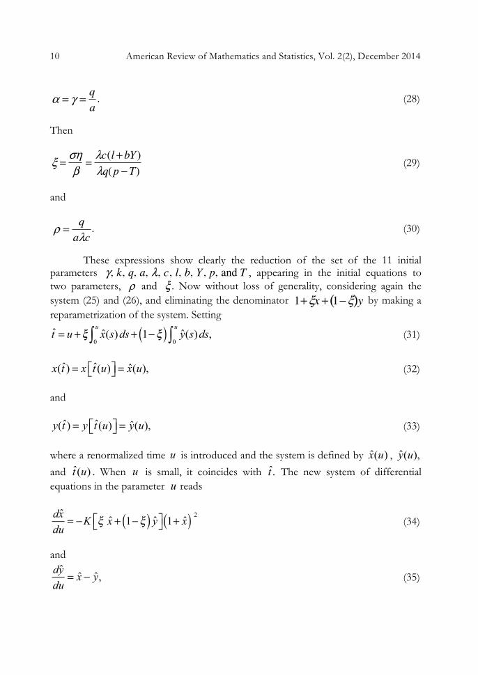
. (28)
Then
(29)
and
. (30)
These expressions show clearly the reduction of the set of the 11 initial
parameters , appearing in the initial equations to two parameters, and . Now without loss of generality, considering again the system (25) and (26), and eliminating the denominator by making a reparametrization of the system. Setting
t = u + ξ x(s)ds+ 1−ξ( ) y(s)ds,
0
u
∫0
u
∫ (31)
x(t ) = x t (u)⎡⎣ ⎤⎦ = x(u), (32) and
y(t ) = y t (u)⎡⎣ ⎤⎦ = y(u), (33) where a renormalized time u is introduced and the system is defined by x(u) , y(u),
and t (u) . When u is small, it coincides with t . The new system of differential equations in the parameter reads
dxdu
= −K ξ x + 1−ξ( ) y⎡⎣ ⎤⎦ 1+ x( ) 2 (34)
and
dydu
= x − y, (35)
α = γ =qa
ξ =σηβ
=λc(l +bY )λq(p −T)
ρ =qaλc
γ, k, q, a, λ, c, l, b, Y, p, and T
ρ
ξ
1+ξx + 1−ξ( )y
u

David S. Torain II 11
where . Therefore, this is the final dimensionless and most simple function
form of the system. Fixed Points In order to study this system in depth, by looking for any fixed points. The first fixed point is x = y = 0 and the second fixed point is
x = −1 and y = −1. (36) In order to study the second fixed point, set
1+ x = x and 1+ y = y. (37) Thus, equations (34) and (35) yields
(38)
and
(39)
So, near and replacing equation (38)
(40)
and integrating equations (39) and (40) yields
(41)
and
y(u) = −e−u ew
Kw+Cdw.
D
u
∫ (42)
Taking the leading terms for large , gives
K =ρξ1− ξ
dx du
= K 1−ξx − (1−ξ)y [ ]x 2
dy du
= x − y .
x = y = 0
dx du
= Kx 2
x (u) = −1
Ku + C
u

12 American Review of Mathematics and Statistics, Vol. 2(2), December 2014
x (u) = − 1
Ku+ o
1u2
⎛⎝⎜
⎞⎠⎟
(43)
and
y(u) = − 1
Ku+ o
1u2
⎛⎝⎜
⎞⎠⎟
. (44)
Equation (44) is obtained by expressing (42) in terms of the transcendent
Ei =
ew
wdw,
1
x
∫ (45)
which for large x behaves like
Ei(x) = ex
x1+ o
1x2
⎡
⎣⎢
⎤
⎦⎥. (46)
So,
y(u) = − 1
Ke− u+C
K⎡⎣⎢
⎤⎦⎥
Ei u + CK
⎛⎝⎜
⎞⎠⎟− Ei D + C
K⎛⎝⎜
⎞⎠⎟
⎡
⎣⎢
⎤
⎦⎥; (47)
therefore, (44). In order to further analyze the behavior near , by eliminating u in (38) to obtain
K 1−ξ x − 1−ξ( ) y⎡⎣ ⎤⎦ x 2 dy
dx= x − y. (48)
Expanding in Taylor series
y x( ) = anx n ,
n = 0
∞
∑ (49)
and identifying powers of in the differential equation, yields
y x( ) = x − K x 2 + o x 3( ). (50)
This series expansion is
1. Valid only if .
2. Asymptotic, that is of zero radius of convergence.
x = y = 0
x
Kx < 0
David S. Torain II 13
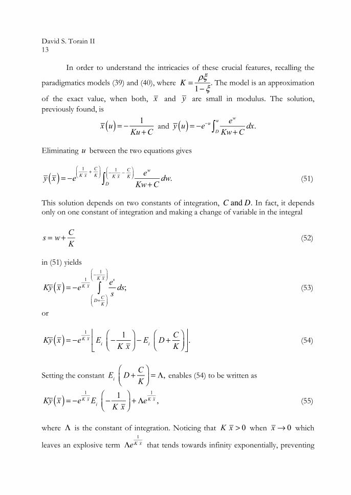
In order to understand the intricacies of these crucial features, recalling the
paradigmatics models (39) and (40), where . The model is an approximation
of the exact value, when both, x and y are small in modulus. The solution, previously found, is
x u( ) = − 1
Ku +C and
y u( ) = −e−u ew
Kw+Cdx.
D
u
∫
Eliminating u between the two equations gives
y x( ) = −e
1K x
+ CK
⎛⎝⎜
⎞⎠⎟ ew
Kw+Cdw.
D
− 1K x
− CK
⎛⎝⎜
⎞⎠⎟∫ (51)
This solution depends on two constants of integration, . In fact, it depends only on one constant of integration and making a change of variable in the integral
s = w+ C
K (52)
in (51) yields
Ky x( ) = −e1
K x es
sds;
D+CK
⎛⎝⎜
⎞⎠⎟
− 1K x
⎛⎝⎜
⎞⎠⎟
∫ (53)
or
Ky x( ) = −e
1K x Ei − 1
K x⎛⎝⎜
⎞⎠⎟− Ei D + C
K⎛⎝⎜
⎞⎠⎟
⎢
⎣⎢
⎥
⎦⎥. (54)
Setting the constant Ei D + C
K⎛⎝⎜
⎞⎠⎟= Λ, enables (54) to be written as
Ky x( ) = −e
1K x Ei − 1
K x⎛⎝⎜
⎞⎠⎟+ Λe
1K x , (55)
where Λ is the constant of integration. Noticing that K x > 0 when x → 0 which
leaves an explosive term Λe1
K x that tends towards infinity exponentially, preventing
K =ρξ1− ξ
C and D
14 American Review of Mathematics and Statistics, Vol. 2(2), December 2014
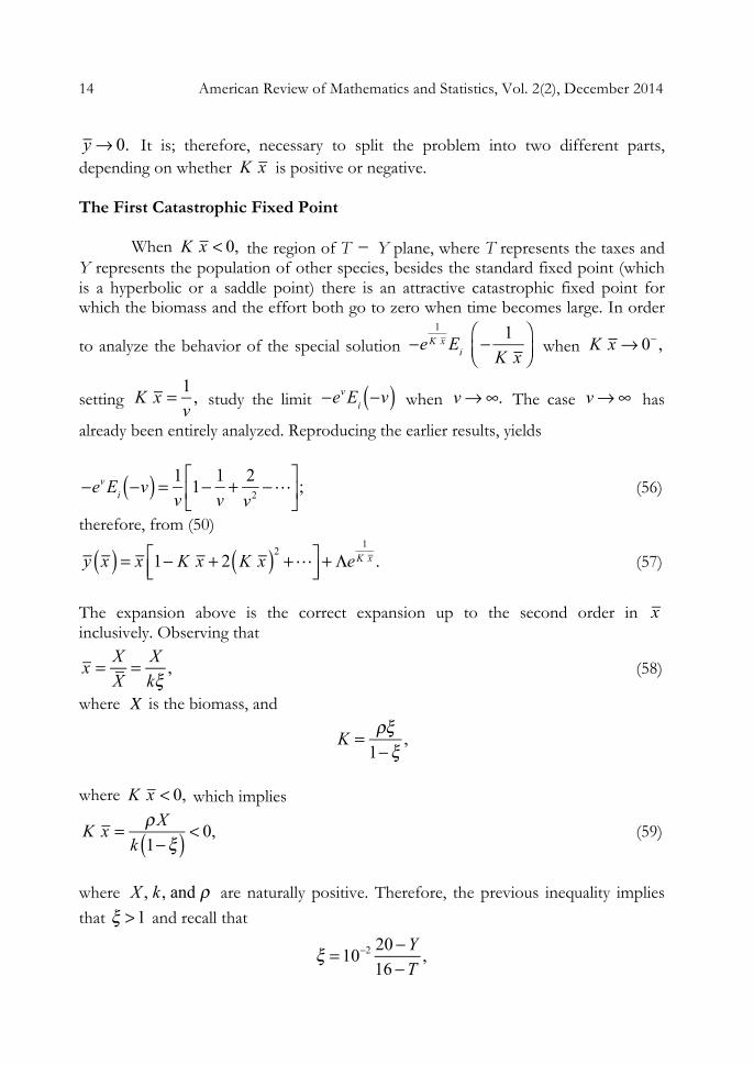
y → 0. It is; therefore, necessary to split the problem into two different parts, depending on whether K x is positive or negative. The First Catastrophic Fixed Point When K x < 0, the region of T − Y plane, where T represents the taxes and Y represents the population of other species, besides the standard fixed point (which is a hyperbolic or a saddle point) there is an attractive catastrophic fixed point for which the biomass and the effort both go to zero when time becomes large. In order
to analyze the behavior of the special solution −e
1K x Ei − 1
K x⎛⎝⎜
⎞⎠⎟
when K x → 0− ,
setting K x = 1
v, study the limit −ev Ei −v( ) when v →∞. The case v →∞ has
already been entirely analyzed. Reproducing the earlier results, yields
−ev Ei −v( ) = 1
v1− 1
v+ 2
v2 −⎡
⎣⎢
⎤
⎦⎥; (56)
therefore, from (50)
y x( ) = x 1− K x + 2 K x( )2
+⎡⎣⎢
⎤⎦⎥ + Λe
1K x . (57)
The expansion above is the correct expansion up to the second order in x inclusively. Observing that
x = X
X= X
kξ, (58)
where is the biomass, and
K = ρξ
1−ξ,
where K x < 0, which implies
K x = ρX
k 1−ξ( ) < 0, (59)
where X , k, and ρ are naturally positive. Therefore, the previous inequality implies that ξ >1 and recall that
ξ = 10−2 20−Y
16−T,
X
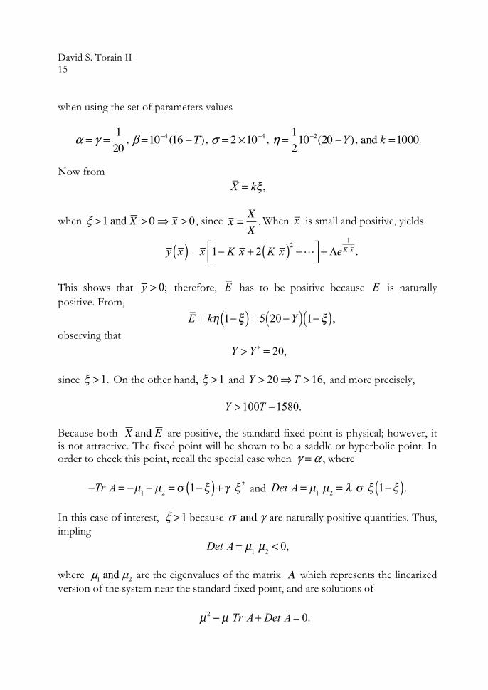
David S. Torain II 15
when using the set of parameters values
.
Now from
X = kξ ,
when
ξ > 1 and X > 0 ⇒ x > 0, since When x is small and positive, yields
y x( ) = x 1− K x + 2 K x( )2
+⎡⎣⎢
⎤⎦⎥ + Λe
1K x .
This shows that y > 0; therefore, E has to be positive because E is naturally positive. From,
E = kη 1−ξ( ) = 5 20−Y( ) 1−ξ( ), observing that
Y > Y ∗ = 20, since ξ >1. On the other hand, ξ >1 and Y > 20⇒T >16, and more precisely,
Y >100T −1580. Because both are positive, the standard fixed point is physical; however, it is not attractive. The fixed point will be shown to be a saddle or hyperbolic point. In order to check this point, recall the special case when , where
−Tr A = −µ1 − µ2 =σ 1−ξ( ) + γ ξ 2 and Det A = µ1 µ2 = λ σ ξ 1−ξ( ). In this case of interest, because are naturally positive quantities. Thus, impling
Det A = µ1 µ2 < 0, where are the eigenvalues of the matrix which represents the linearized version of the system near the standard fixed point, and are solutions of
µ2 − µ Tr A+ Det A = 0.
α = γ =120
, β = 10−4 (16 −T), σ = 2 ×10⁻⁴, η =12
10−2(20 −Y), and k = 1000
x =XX .
X and E
γ = α
ξ >1
σ and γ
µ1 and µ2
A

16 American Review of Mathematics and Statistics, Vol. 2(2), December 2014 Introducing the discriminant
Δ = Tr A( )2
− 4Det A = σ 1−ξ( ) + γ ξ 2⎡⎣ ⎤⎦2−4γ σ ξ 1−ξ( ),
when , produces two real roots of opposite sign. This is a hyperbolic fixed point (saddle). So, there is only one attractive (catastrophic) fixed point. Finally, given the asymptotic relation between the pseudo-time u and the dimensionless time
t for large u, without approximation,
dxdu
= K 1−ξ x − 1−ξ( ) y⎡⎣ ⎤⎦ x 2 , dydu
= x − y ,
and
t = y(s)ds+ ξ y(u)− y(0)( ).
0
u
∫ (60)
Or, the lowest order, when are simultaneously small,
,
and
t = y(s)ds+ ξ y(u)− y(0)( ).
0
u
∫
Integrate to obtain
y = 1
−Ku +C+ o
1u2
⎛⎝⎜
⎞⎠⎟
,
t = 1
−Klnu + o(1) as u→∞ and K < 0.
In summary, when
Y >100T −1580 and T >16, there is an attractive catastrophic fixed point for which the biomass and the effort both go to zero exponentially fast when time becomes large, while the standard fixed
ξ > 1 and Δ < 0
x and y
dx du
= Kx 2, dy du
= x − y
x =1
−Ku + C,
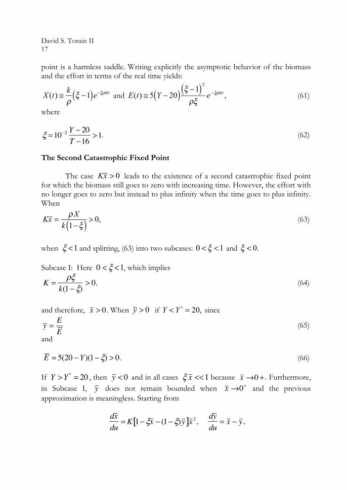
David S. Torain II 17
point is a harmless saddle. Writing explicitly the asymptotic behavior of the biomass and the effort in terms of the real time yields:
X (t) ≅ k
ρξ −1( )e−ξρσ t and
E(t) ≅ 5 Y − 20( ) ξ −1( )2
ρξe−ξρσ t , (61)
where
. (62)
The Second Catastrophic Fixed Point The case Kx > 0 leads to the existence of a second catastrophic fixed point for which the biomass still goes to zero with increasing time. However, the effort with no longer goes to zero but instead to plus infinity when the time goes to plus infinity. When
Kx = ρX
k 1−ξ( ) > 0, (63)
when and splitting, (63) into two subcases: 0 < ξ <1 and ξ < 0. Subcase I: Here , which implies
(64)
and therefore, When y > 0 if Y < Y ∗ = 20, since
(65)
and
. (66) If , then and in all cases because . Furthermore, in Subcase I, does not remain bounded when and the previous approximation is meaningless. Starting from
,
ξ =10−2 Y −20T −16
>1
ξ <1
0 < ξ <1
K =ρξ
k(1− ξ)> 0,
x > 0.
y =EE
E = 5(20 −Y)(1−ξ) > 0
Y >Y * = 20
y < 0
ξ x << 1
x →0+
y
x →0+
dx du
= K 1−ξx − (1−ξ)y [ ]x 2, dy du
= x − y
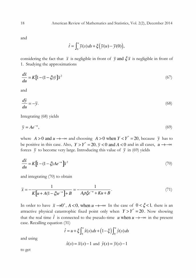
18 American Review of Mathematics and Statistics, Vol. 2(2), December 2014 and
t = y(s)ds+ ξ y(u)− y(0)( ),
0
u
∫
considering the fact that is negligible in front of is negligible in front of 1. Studying the approximations
(67)
and
. (68)
Integrating (68) yields
, (69) where and choosing , because has to be positive in this case. Also, and in all cases, forces to become very large. Introducing this value of in (69) yields
(70)
and integrating (70) to obtain
. (71)
In order to have In the case of there is an attractive physical catastrophic fixed point only when . Now showing that the real time t is connected to the pseudo-time in the present case. Recalling equation (31)
t = u + ξ x(s)ds+ 1−ξ( ) y
0
u
∫ (s)ds0
u
∫
and using
x(s) = x (s)−1 and y(s) = y(s)−1 to get
x
y and ξ x
dx du
= K 1− (1−ξ)y [ ]x 2
dy du
= −y
y = Ae−u
A > 0 and u→−∞
A > 0 when Y <Y * = 20
y
Y > Y * = 20, y < 0 and A < 0
u→−∞
y
y
dx du
= K 1− (1−ξ)Ae−u[ ]x 2
x = −1
K u + A(1−ξ)e−u[ ]+ B= −
1Aρξe−u + Ku + B
x →0+, A < 0, when u →−∞.
0 < ξ <1,
Y >Y * = 20
u when u→−∞

David S. Torain II 19
t = u + ξ x (s)−1( )ds+ 1−ξ( ) y(s)−1( )ds.
0
u
∫0
u
∫ (72)
Using the exact equation
and substitute , where
(73)
in the relation between the real time t and the pseudo-time u. Then, the relation between the real time t and the pseudo-time u can be written as
t = ξ y(u)− y(0)( ) + y(s)ds
0
u
∫ (74)
and
, (75) where is valid for large . In order to find the asymptotic relation between the real time t and the pseudo-time u, when , and only keeping the leading terms, to obtain
t ≅ ξAe−u + A e−s ds = − 1−ξ( )Ae−u = 1−ξ( ) A e−u ,
Λ
u
∫ (76)
Now, expressing the behavior of the biomass and fishing effort in this case T >16, (77)
, (78)
X ≅ k
ρ σ t, (79)
and
. (80)
The biomass goes to zero as the inverse of the real time; therefore, it goes slowly. Also, the fishing effort goes to infinity linearly in the real time and therefore, slowly. In this case, the standard fixed point is unphysical since
dy du
= x − y
x (s)
x (s) = y (s)+dy (s)
ds,
y (u) ≅ Ae−u
u→−∞
u
u→−∞
20 <Y <100T −1580
E ≅5σ (Y −20)100(T −16)
(100T −1580 −Y)t

20 American Review of Mathematics and Statistics, Vol. 2(2), December 2014
. (81) There is no competition between attractive fixed points in this case. Global Description of the Fixed Points in the Plane Summary of the Situation I-1. Existence and nature of the “standard” fixed point. In order for the standard fixed point to exist, it is necessary that both
(82) and
, (83)
where
η =
b a
l b
−Y⎛
⎝⎜
⎞
⎠⎟ =
b a
Y ∗ −Y( ) and that
k, a, and l , are naturally positive
quantities with two possible cases: Case A:
0 < ξ <1 and 0 < Y < Y ∗ = 20 (84) Case B:
ξ >1 and Y > Y ∗ = 20. (85) I-2. Stability of the standard fixed point.
I-2-1. Case A is subdivided into tree subcases:
A1. 0 < ξ < 0.00099 and 0 < Y < Y ∗ = 20, for which a knot and asymptotic stability. (Blue region in the plane Figure 1)
E = 5(20 −Y)(1−ξ) < 0
T −Y
X , E ( )
X = kξ > 0
E = kη(1−ξ) > 0
T −Y

David S. Torain II 21
A2. 0.001< ξ < 0.22848 and 0 < Y < Y ∗ = 20, for which a focus and counterclockwise spiral attractor. (Green region in the plane Figure 1)
A3. 0.22849 < ξ <1 and 0 < Y < Y ∗ = 20, for which a knot and asymptotic
stability. (Blue region in the plane Figure 1)
I-2-2 Case B is the linearized equations from matrix
A , where
−Tr A =σ 1−ξ( ) + γ ξ 2 ,
Det A = γ σ ξ 1−ξ( ) < 0,
and
Δ = Tr A( )2 − 4Det A > 0 . The discriminant is positive; hence, the roots are real. The determinant is the negative product of roots, one positive, and the other negative. Therefore, this an asymptotic instability with a saddle point.
II. Existence and nature of the “catastrophic” fixed point with three cases:
ξ < 0, ξ >1, and 0 < ξ <1.
II-1. , recalling Y > Y ∗ = 20 and T < T ∗ = 16, for which a stable catastrophic fixed point in which the biomass goes to zero as the inverse of the time and the effort goes to infinity linearly in time. (White region in the T – Y plane Figure 1)
The first fixed point does not exist in this case because it is unphysical, thus implying a negative biomass. Therefore, there is no competition between the two fixed points.
II-2. , recalling T > T ∗ = 16 and Y >100T −1580 with 0 < Y , for which a stable catastrophic fixed point, with the biomass and the effort going to zero exponentially fast with time. (Yellow region in the plane Figure 1)
T −Y
T −Y
Δ
ξ < 0
ξ >1
T −Y
22 American Review of Mathematics and Statistics, Vol. 2(2), December 2014
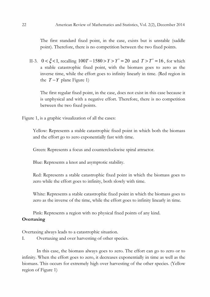
The first standard fixed point, in the case, exists but is unstable (saddle point). Therefore, there is no competition between the two fixed points.
II-3. , recalling 100T −1580 > Y > Y ∗ = 20 and T > T ∗ = 16 , for which a stable catastrophic fixed point, with the biomass goes to zero as the inverse time, while the effort goes to infinity linearly in time. (Red region in the plane Figure 1)
The first regular fixed point, in the case, does not exist in this case because it
is unphysical and with a negative effort. Therefore, there is no competition between the two fixed points.
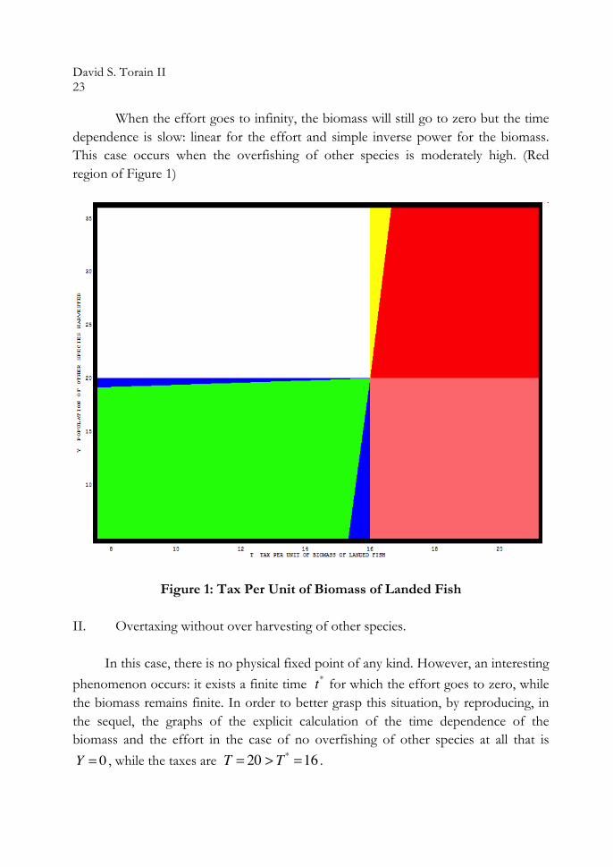
Figure 1, is a graphic visualization of all the cases:
Yellow: Represents a stable catastrophic fixed point in which both the biomass and the effort go to zero exponentially fast with time.
Green: Represents a focus and counterclockwise spiral attractor.
Blue: Represents a knot and asymptotic stability. Red: Represents a stable catastrophic fixed point in which the biomass goes to zero while the effort goes to infinity, both slowly with time. White: Represents a stable catastrophic fixed point in which the biomass goes to zero as the inverse of the time, while the effort goes to infinity linearly in time. Pink: Represents a region with no physical fixed points of any kind.
Overtaxing Overtaxing always leads to a catastrophic situation. I. Overtaxing and over harvesting of other species.
In this case, the biomass always goes to zero. The effort can go to zero or to infinity. When the effort goes to zero, it decreases exponentially in time as well as the biomass. This occurs for extremely high over harvesting of the other species. (Yellow region of Figure 1)
0 < ξ <1
T −Y
David S. Torain II 23
When the effort goes to infinity, the biomass will still go to zero but the time dependence is slow: linear for the effort and simple inverse power for the biomass. This case occurs when the overfishing of other species is moderately high. (Red region of Figure 1)
Figure 1: Tax Per Unit of Biomass of Landed Fish II. Overtaxing without over harvesting of other species.
In this case, there is no physical fixed point of any kind. However, an interesting phenomenon occurs: it exists a finite time for which the effort goes to zero, while the biomass remains finite. In order to better grasp this situation, by reproducing, in the sequel, the graphs of the explicit calculation of the time dependence of the biomass and the effort in the case of no overfishing of other species at all that is
, while the taxes are .
t*
Y = 0
T = 20 > T* =16

24 American Review of Mathematics and Statistics, Vol. 2(2), December 2014 Considering two different initial values:
(1) At time , the biomass = 0.5 and the effort = 0.5 of the standard fixed
point values. This produces a critical time , in dimensionless units, for which the effort goes to zero, while the biomass still remains finite a little below six. (Figure 2)
Figure 2: Effect of Overtaxing: Biomass = .5 and Effort = .5 (2) At time , the biomass = 0.3 and the effort = 1.1 of the standard fixed
point values. This produces a critical time in dimensionless units, for which the effort goes to zero, while the biomass still remains finite. (Figure 3)
t = 0
t* = 0.4
t = 0
t* =1.1

David S. Torain II 25
Figure 3: Effect of Overtaxing: Biomass = .3 and Effort = 1.1 * Noting that any negative effort is a result of the high increase effort in community contribution [9].

26 American Review of Mathematics and Statistics, Vol. 2(2), December 2014 Conclusion
The objective of this paper has been achieved: to be able, using “Dimensional Analysis,” to get an overview of a Mathematical Model. Overview is an intension to classify the different solutions that could occur in different situations. More interesting, the “Dimensional Analysis” allows the possibility to understand all the solutions of the model and all its weaknesses. Among the most classical weaknesses are parametric regions that produce unboundedness of physical quantities or non-positive solutions when for obvious reasons have to be positive. This kind of positivity and/or bounded requirements can be embedded from start in the equations by using standard methods that can be found in the reference book [8].
Dimensional Analysis gave a global view of the different kind of classes of solutions (positive, non-positive, bounded, unbounded, and etcetera) that cannot be given by computer calculations. The equations depend on sixteen parameters and it is necessary to fix all of them in order to get a computer solution. Taking the exact opposite approach and letting all of the parameters be free, thus, obtaining a panoramic view of all possible solutions.
Using “Dimensional Analysis,” a tool never used before in Mathematical
Models, help to analize the full model, which depended on sixteen parameters. Reducing the parameters, in all generality and rigor, to three dimensionless parameters out of which only one called plays a crucial and dominant role. The parameter divides the parametric space into seven regions that can grossly be described by the presence of different fixed points and different classes of solutions corresponding to over or under harvesting of other species, over or under taxing etcetera. Each of these regions defines a class of solutions in Figure 1, having the same behavior. The analysis of these classes allows for detection of some limitations of the model. In some classes, the biomass may become negative or unbounded; in other classes, negative effort may appear instead.
ξ
ξ

David S. Torain II 27
References Holmes B., Biologists sort the lessons of fisheries collapse, Science, 264 (1994), pp. 1252-
1253. Tibbetts J., Ocean commotion, Environmental Health Perspectives, 104 (1994), pp. 380-385. Burkholder JoAnn M., Implications of Harmful Microalgae and Heterotrophic Dinoflagellates
in Mansgement of Sustainable Marine Fisheries, Ecological Applications, 8(1) Supplement, (1998), pp. S37-S62.
Burkholder JoAnn M., and Glasgow Howard B Jr., Pfiesteria piscicda and other Pfiesteria-like dinoflagellates: Behavior, impacts, and environmental controls, American Society of Limnol. Oceanogr., 42(5, part 2), (1997), pp. 1052-1075.
Chaudhuri Kripasindhu., and Johnson Thomas., Bioeconomic Dynamics of a Fishery Modeled as an S-System, Mathematical Biosciences an international journal, 99 (1990), pp. 231-249.
Clark C. W., Mathematical Bioeconomics: The Optimal Management of Renewable Resources, John Wiley & Sons, New York, (1976).
Chaudhuri Kripasindhu., Private Communication, (2005) Thieme R. Horst; Mathematics in Population Biology in The Princeton Series in Theoretical
and Computational Biology, ISBN 0-691-09291-5, (2003). Greenville W. Jared., and MacAulay T. G., A Bioeconomic Model of a MarinePark,
Agricultural and Resource Economics, University of Sydney, NSW, (2006).