A Critique of Software Defect PredictionModels

Norman Fenton

Martin Neil

Centre for Software Reliability

Northampton Square

London EC1V 0HB

Abstract: Many organisations want to predict the number of defects (faults)in software systems, before they are deployed, to gauge the likely deliveredquality and maintenance effort. To help in this numerous software metrics andstatistical models have been developed, with a correspondingly largeliterature. We provide a critical review of this literature and the state-of-the-art. Most of the wide range of prediction models use size and complexitymetrics to predict defects. Others are based on testing data, the ‘quality’ of thedevelopment process, or take a multivariate approach. The authors of themodels have often made heroic contributions to a subject otherwise bereft ofempirical studies. However, there are a number of serious theoretical andpractical problems in many studies. The models are weak because of theirinability to cope with the, as yet, unknown relationship between defects andfailures. There are fundamental statistical and data quality problems thatundermine model validity. More significantly many prediction models tend tomodel only part of the underlying problem and seriously mis-specify it. Toillustrate these points the ‘Goldilock’s Conjecture’, that there is an optimummodule size, is used to show the considerable problems inherent in currentdefect prediction approaches. Careful and considered analysis of past and newresults shows that the conjecture lacks support and that some models aremisleading. We recommend holistic models for software defect prediction,using Bayesian Belief Networks, as alternative approaches to the single-issuemodels used at present. We also argue for research into a theory of ‘softwaredecomposition’ in order to test hypotheses about defect introduction and helpconstruct a better science of software engineering.

1 Introduction

Organisations are still asking how they can predict the quality of their software before it isused despite the substantial research effort spent attempting to find an answer to this questionover the last 30 years. There are hundreds of papers advocating statistical models and metrics

which purport to answer the quality question. Defects, like quality, can be defined in manydifferent ways but are more commonly defined as deviations from specifications orexpectations which might lead to failures in operation.

Generally, efforts have tended to concentrate on the following three problem perspectives[Schneidewind & Hoffmann 1979, Potier et. al. 1982, Nakajo & Kume 1991]:

• predicting the number of defects in the system;

• estimating the reliability of the system in terms of time to failure;

• understanding the impact of design and testing processes on defect counts and failuredensities.

A wide range of prediction models have been proposed. Complexity and size metrics havebeen used in an attempt to predict the number of defects a system will reveal in operation ortesting. Reliability models have been developed to predict failure rates based on the expectedoperational usage profile of the system. Information from defect detection and the testingprocess has been used to predict defects. The maturity of design and testing processes havebeen advanced as ways of reducing defects. Recently large complex multivariate statisticalmodels have been produced in an attempt to find a single complexity metric that will accountfor defects.

This paper provides a critical review of this literature with the purpose of identifying futureavenues of research. We cover complexity and size metrics (Section 2), the testing process(Section 3), the design and development process (Section 4) and recent multivariate studies(Section 5). For a comprehensive discussion of reliability models, see [Brocklehurst &Littlewood 1992]. We uncover a number of theoretical and practical problems in thesestudies in Section 6, in particular the so-called ‘Goldilock’s Conjecture’.

Despite the many efforts to predict defects there appears to be little consensus on what theconstituent elements of the problem really are. In Section 7 we suggest a way to improve thedefect prediction situation by describing a prototype, Bayesian Belief Network (BBN) based,model which we feel can at least partly solve the problems identified. Finally, in Section 8we record our conclusions.

2 Prediction using size and complexity metrics

Most defect prediction studies are based on size and complexity metrics. The earliest suchstudy appears to have been [Akiyama 1971] which was based on a system developed atFujitsu, Japan. It is typical of many regression based ‘data fitting’ models which becamecommon-place in the literature. The study showed that linear models of some simple metricsprovide reasonable estimates for the total number of defects D (the dependent variable)which is actually defined as the sum of the defects found during testing and the defects foundduring two months after release. Akiyama computed four regression equations.

The equation (1) involving lines of code L (LOC) was so that, for example, a 1000 LOC (i.e.1 KLOC) module is expected to have about 23 defects:

D = . + . L4 86 0 018 (1)

Other equations had the following dependent metrics: Number of decisions C; Number ofsubroutine calls J; and a composite metric C+J.

Another early study [Ferdinand 1974] argued that the expected number of defects increaseswith the number n of code segments; a code segment is a sequence of executable statementswhich, once entered, must all be executed. Specifically the theory asserts that for smallernumbers of segments, the number of defects is proportional to a power of n; for largernumbers of segments, the number of defects increases as a constant to the power n.

[Halstead 1975] proposed a number of size metrics, which have been interpreted as‘complexity’ metrics, and used these as predictors of program defects. Most notably,Halstead asserted that the number of defects D in a program P is predicted by (2):

D = V

3000(2)

where V is the (language dependent) volume metric (which like all the Halstead metrics isdefined in terms of number of unique operators and unique operands in P; for details see[Fenton & Kitchenham 1991]). The divisor 3000 represents the mean number of mentaldiscriminations between decisions made by the programmer. Each such decision possiblyresults in error and thereby a residual defect. Thus, Halstead's model was, unlike Akiyama's,based on some kind of theory. Interestingly, Halstead himself "validated" (1) usingAkiyama's data. [Ottenstein 1979] obtained similar results to Halstead.

[Lipow 1982] went much further, because he got round the problem of computing V directlyin (3), by using lines of executable code L instead. Specifically, he used the Halstead theoryto compute a series of equations of the form:

D

L = A + a L + A L0 1 2

2ln ln (3)

where each of the Ai are dependent on the average number of usages of operators andoperands per LOC for a particular language. For example, for Fortran A0 = 0.0047; A1 =0.0023; A2 = 0.000043. For an assembly language A0 = 0.0012; A1 = 0.0001; A2 = 0.000002.

[Gaffney 1984] argued that the relationship between D and L was not language dependent.He used Lipow's own data to deduce the prediction (4):

D = . + . (L) /4 2 0 0015 4 3 (4)

An interesting ramification of this was that there was an optimal size for individual moduleswith respect to defect density. For (4) this optimum module size is 877 LOC. Numerous

other researchers have since reported on optimal module sizes. For example, [Compton &Withrow 1990] of UNISYS derived the following polynomial regression equation:

D = . + . L + . (L)0 069 0 00156 0 00000047 2 (5)

Based on (5) and further analysis Compton and Withrow concluded that the optimum size foran Ada module, with respect to minimising error density is 83 source statements. Theydubbed this the ‘Goldilocks Principle’ with the idea that there is an optimum module sizethat is “not too big nor too small”.

The phenomenon that larger modules can have lower defect densities was confirmed [Basili& Perricone 1984], [Shen 1985], and [Moller & Paulish 1993]. Basili and Perricone arguedthat this may be explained by the fact that there are a large number of interface defectsdistributed evenly across modules. Moller and Paulish suggested that larger modules tend tobe developed more carefully; they discovered that modules consisting of greater than seventylines of code have similar defect densities. For modules of size less than seventy lines ofcode, the defect density increases significantly.

Similar experiences are reported by [Hatton 1993, 1994]. Hatton examined a number of datasets [Keller 1992, Moller & Paulish 1993] and concluded that there was evidence of‘macroscopic behaviour’ common to all data sets despite the massive internal complexity ofeach system studied, [Hatton 1997]. This behaviour was likened to ‘molecules’ in a gas andused to conjecture an entropy model for defects which also borrowed from ideas in cognitivepsychology. Assuming the short-term memory affects the rate of human error he developed alogarithmic model, made up of two parts, and fitted it to the data sets1. The first partmodelled the effects of small modules on short-term memory, while the second modelled theeffects of large modules. He asserted that, for module sizes above 200-400 lines of code, thehuman ‘memory cache’ overflows and mistakes are made leading to defects. For systemsdecomposed into smaller pieces than this cache limit the human memory cache is usedinefficiently storing ‘links’ between the modules thus also leading to more defects. Heconcluded that larger components are proportionally more reliable than smaller components.Clearly this would, if true, cast serious doubt over the theory of program decompositionwhich is so central to software engineering.

The realisation that size-based metrics alone are poor general predictors of defect densityspurred on much research into more discriminating complexity metrics. McCabe'scyclomatic complexity, [McCabe 1976], has been used in many studies, but it too isessentially a size measure (being equal to the number of decisions plus one in mostprograms). [Kitchenham et. al. 1990] examined the relationship between the changes

1 There is nothing new here since [Halstead 1975] was one of the first to apply Miller’s finding that

people can only effectively recall 7 plus or minus 2 items from their short-term memory. Likewise

the construction of a partitioned model contrasting ‘small’ module effects on faults and ‘large’

module effects on faults was done by Compton and Withrow in 1990 [Compton & Withrow 1990].

experienced by two sub-systems and a number of metrics, including McCabe's metric. Twodifferent regression equations resulted (6), (7):

C = . MCI - . N + . HE 0 042 0 075 0 00001 (6)

C = . MCI - . DI + . VG0 25 053 0 09 (7)

For the first sub-system changes, C, was found to be reasonably dependent on machine codeinstructions, MCI, operator and operand totals, N, and Halstead's effort metric, HE. For theother sub-system McCabe's complexity metric, VG was found to partially explain C alongwith machine code instructions, MCI and data items, DI.

All of the metrics discussed so far are defined on code. There are now a large number ofmetrics available earlier in the life-cycle, most of which have been claimed by theirproponents to have some predictive powers with respect to residual defect density. Forexample, there have been numerous attempts to define metrics which can be extracted fromdesign documents using counts of ‘between module complexity’ such as call statements anddata flows; the most well known are the metrics in [Henry & Kafura 1984]. [Ohlsson andAlberg 1996] reported on a study at Ericsson where metrics derived automatically fromdesign documents were used to predict especially fault-prone modules prior to testing.Recently, there have been several attempts, such as [Basili et. al. 1996] and [Chidamber &Kemerer 1992], to define metrics on object-oriented designs.

The advent and widespread use of Albrecht Function Points (FPs) raises the possibility ofdefect density predictions based on a metric which can be extracted at the specification stage.There is widespread belief that FPs are a better (one-dimensional) size metric than LOC; intheory at least they get round the problems of lack of uniformity and they are also languageindependent. We already see defect density defined in terms of defects per FP, and empiricalstudies are emerging that seem likely to be the basis for predictive models. For example, inTable 1, [Jones 1991] reports the following bench-marking study, reportedly based on largeamounts of data from different commercial sources.

Defect Origins Defects per Function Point

Requirements 1.00

Design 1.25

Coding 1.75

Documentation 0.60

Bad Fixes 0.40

Total 5.00

Table 1: Defects per life-cycle phase

3 Prediction using testing metrics

Some of the most promising local models for predicting residual defects involve very carefulcollection of data about defects discovered during early inspection and testing phases. Theidea is very simple: you have n pre-defined phases at which you collect data dn the defectrate. Suppose phase n represents the period of the first 6 months of the product in the field,so that dn is the rate of defects found within that period. To predict dn at phase n-1 (whichmight be integration testing) you look at the actual sequence d1,...,dn-1 and compare this withprofiles of similar, previous products, and use statistical extrapolation techniques. Withenough data it is possible to get accurate predictions of dn based on observed d1,...,dm wherem is less than n-1. This method is an important feature of the Japanese software factoryapproach [Cusomano 1991, Koga 1992, Yasuda 1989]. Extremely accurate predictions areclaimed (usually within 95% confidence limits) due to stability of the development andtesting environment and the extent of data-collection. It appears that the IBM NASA Spaceshuttle team is achieving similarly accurate predictions based on the same kind of approach[Keller 1992].

In the absence of an extensive local database it may be possible to use published bench-marking data to help with this kind of prediction. [Dyer 1992] and [Humphrey 1989],contain a lot of this kind of data. [Buck & Robbins 1984] report on some remarkablyconsistent defect density values during different review and testing stages across differenttypes of software projects at IBM. For example, for new code developed the number ofdefects per KLOC discovered with Fagan inspections settles to a number between 8 and 12.There is no such consistency for old code. Also the number of man-hours spent on theinspection process per major defect is always between 3 and 5. The authors speculate that,despite being unsubstantiated with data, these values form ‘natural numbers ofprogramming’, believing that they are 'inherent to the programming process itself'. Alsouseful (providing you are aware of the kind of limitations discussed in [Fenton et. al. 1994])is the kind of data published by [Grady 1992] in the Table 2:

Testing Type Defectsfound per

hour

Regular use 0.210

Black-box 0.282

White-box 0.322

Reading/Inspections 1.057

Table 2: Defects found per testing approach

One class of testing metrics that appear to be quite promising for predicting defects are the socalled test coverage measures. A structural testing strategy specifies that we have to selectenough test cases so that each of a set of "objects" in a program lie on some path (i.e. are‘covered’) in at least on test case. For example, statement coverage is a structural testingstrategy in which the "objects" are the statements. For a given strategy and a given set of test

cases we can ask what proportion of coverage has been achieved. The resulting metric isdefined as the Test Effectiveness Ratio (TER) with respect to that strategy. For exampleTER1 is the TER for statement coverage; TER2 is the TER for branch coverage; and TER3is the TER for Linear Code Sequence and Jump coverage. Clearly we might expect thenumber of discovered defects to approach the number of defects actually in the program asthe values of these TER metrics increases. [Veevers & Marshall 1994] report on some defectand reliability prediction models using these metrics which give quite promising results.Interestingly [Neil 1992b] reported that the modules with high structural complexity metricvalues had a significantly lower TER than smaller modules. This supports our intuition thattesting larger modules is more difficult and that such modules would appear more likely tocontain undetected defects.

Voas and Miller use static analysis of programs to conjecture the presence or absence ofdefects before testing has taken place [Voas & Miller 1995]. Their method relies on a notionof program testability which seeks to determine how likely a program will fail assuming itcontains defects. Some programs will contain defects that may be difficult to discover bytesting by virtue of their structure and organisation. Such programs have a low defectrevealing potential and may therefore hide defects until they show themselves as failuresduring operation. Voas and Miller use program mutation analysis to simulate the conditionsthat would cause a defect to reveal itself as a failure if a defect was indeed present.Essentially if program testability could be estimated before testing takes place the estimatescould help predict those programs that would reveal less defects during testing even if theycontained defects. [Bertolino & Strigini 1996] provide an alternative exposition of testabilitymeasurement and its relation to testing, debugging and reliability assessment.

4 Prediction using process quality data

There are many experts who argue that the ‘quality’ of the development process is the bestpredictor of product quality (and hence, by default, of residual defect density). This issue,and the problems surrounding it, is discussed extensively in [Fenton et. al. 1994]]. There is adearth of empirical evidence linking process quality to product quality. The simplest metricof process quality is the 5-level ordinal scale SEI Capability Maturity Model (CMM)ranking. Despite its widespread popularity, there was until recently no evidence to show thatlevel(n+1) companies generally deliver products with lower residual defect density thanlevel(n) companies. The [Diaz & Sligo 1997] study provides the first promising empiricalsupport for this widely held assumption.

Clearly the strict 1-5 ranking, as prescribed by the SEI-CMM, is too coarse to be useddirectly for defect prediction since not all of the processes covered by the CMM will relate tosoftware quality. The best available evidence relating particular process methods to defectdensity concerns the Cleanroom method [Dyer 1992]. There is independent validation that,for relatively small projects (less than 30 KLOC), the use of Cleanroom results inapproximately 3 errors per KLOC during statistical testing, compared with traditionaldevelopment post-delivery defect densities of between 5 to 10 defects per KLOC. Also,Capers Jones hypothesises quality targets expressed in ‘defect potentials’ and ‘delivereddefects’ for different CMM levels, as shown in Table 3, [Jones 1996].

SEI CMM Levels Defect Potentials Removal Efficiency Delivered Defects

1 5 85% 0.75

2 4 89% 0.44

3 3 91% 0.27

4 2 93% 0.14

5 1 95% 0.05

Table 3: Relationship between CMM levels and delivered defects

5 Multivariate approaches

There have been many attempts to develop multi-linear regression models based on multiplemetrics. If there is a consensus of sorts about such approaches it is that the accuracy of thepredictions is never significantly worse when the metrics set is reduced to a handful (say 3-6rather than 30) [Munson & Khoshgoftaar 1990]. A major reason for this is that many of themetrics are collinear; that is they capture the same underlying attribute so the reduced setof metrics has the same information content, [Neil 1992a]. Thus, much work hasconcentrated on how to select those small number of metrics which are somehow the mostpowerful and/or representative. Principal Component Analysis (see [Manly 1986]) is used insome of the studies to reduce the dimensionality of many related metrics to a smaller set of‘principal components’, whilst retaining most of the variation observed in the originalmetrics.

For example, [Neil 1992a] discovered that 38 metrics, collected on around 1000 modules,could be reduced to 6 orthogonal dimensions that account for 90% of the variability. Themost important dimensions; size, nesting and prime were then used to develop an equation todiscriminate between low and high maintainability modules.

Munson and Khoshgoftaar in various papers, [Khoshgoftaar & Munson 1990, Munson &Khoshgoftaar 1990, 1992], use a similar technique, Factor Analysis, to reduce thedimensionality to a number of “independent” factors. These factors are then labelled so as torepresent the ‘true’ underlying dimension being measured, such as control, volume andmodularity. In [Khoshgoftaar & Munson 1990] they used factor analytic variables to help fitregression models to a number of error data sets, including Akiyama's [Akiyama 1971]. Thishelped to get over the inherent regression analysis problems presented by multicollinearity inmetrics data.

Munson and Khoshgoftaar have advanced the multivariate approach to calculate a ‘relativecomplexity metric’. This metric is calculated using the magnitude of variability from each ofthe factor analysis dimensions as the input weights in a weighted sum. In this way a singlemetric integrates all of the information contained in a large number of metrics. This is seento offer many advantages of using a univariate decision criterion such as McCabe's metric[Munson & Khoshgoftaar 1992].

6 A critique of current approaches to defect prediction

One could be forgiven for inferring from the sheer volume of research and practical workdone in software defect prediction that the underlying problem had been largely solved.Unfortunately nothing could be further from the truth. There are some flawed assumptionsabout how defects are defined, caused and observed and this has led to contradictoryconclusions and false claims. Many of the empirical results reported about defects and thefactors that shape their introduction and detection are weakened by potentially fatal flawseither in the research methodology and theory used or the data collected.

In order to best suggest improvements to the software engineering community’s researchdirection we classify the serious problems as follows (dealing with each in turn in subsequentsections)

• the unknown relationship between defects and failures (Section 6.1);

• problems with the ‘multivariate’ statistical approach (Section 6.2);

• problems of using size and complexity metrics as sole ‘predictors’ of defects(Section 6.3);

• problems in statistical methodology and data quality (Section 6.4);

• false claims about software decomposition and the ‘Goldilock’s conjecture’(Section 6.5).

6.1 The Unknown Relationship between Defects and Failures

There is considerable disagreement about the definitions of defects, errors, faults andfailures. In different studies defect counts refer to:

• post-release defects;

• the total of "known" defects;

• the set of defects discovered after some arbitrary fixed point in the software life-cycle(e.g. after unit testing).

The terminology differs widely between studies; defect rate, defect density and failure rateare used almost interchangeably. It can also be difficult to tell whether a model is predictingdiscovered defects or residual defects. Because of these problems (which are discussedextensively in [Fenton & Pfleeger 1996]) we have to be extremely careful about the way weinterpret published predictive models.

Apart from these problems of terminology and definition the most serious weakness of anyprediction of residual defects or defect density concerns the weakness of defect count itself

as a measure of software reliability2. Even if we knew exactly the number of residual defectsin our system we have to be extremely wary about making definitive statements about howthe system will operate in practice. The reasons for this appear to be:

• Difficulty of determining in advance the seriousness of a defect; few of the empiricalstudies attempt to distinguish different classes of defects;

• Great variability in the way systems are used by different users, resulting in widevariations of operational profiles. It is thus difficult to predict which defects are likelyto lead to failures (or to commonly occurring failures).

The latter point is particularly serious and has been highlighted dramatically by [Adams1984]. Adams examined data from nine large software products, each with many thousandsof years of logged use world-wide. He charted the relationship between detected defects andtheir manifestation as failures. For example, 33% of all defects led to failures with a meantime to failure greater than 5000 years. In practical terms, this means that such defects willalmost never manifest themselves as failures. Conversely, the proportion of defects whichled to a mean time to failure of less than 50 years was very small (around 2%). However, itis these defects which are the important ones to find, since these are the ones whicheventually exhibit themselves as failures to a significant number of users. Thus, Adams' datademonstrates the Pareto principle: a very small proportion of the defects in a system will leadto almost all the observed failures in a given period of time; conversely, most defects in asystem are benign in the sense that in the same given period of time they will not lead tofailures.

It follows that finding (and removing) large numbers of defects may not necessarily lead toimproved reliability. It also follows that a very accurate residual defect density predictionmay be a very poor predictor of operational reliability, as has been observed in practice[Fenton & Ohlsson 1997]. This means we should be very wary of attempts to equate faultdensities with failure rates, as proposed for example by Capers Jones (Table 4, cited in[Stalhane 1992]). Although highly attractive in principle, such a model does not stand up toempirical validation.

F/KLOC MTTF

> 30 1 minute

20 -30 4-5 minutes

5 - 10 1 hour

2 - 5 several hours

2 Here we use the ‘technical’ concept of reliability, defined as mean time to failure or probability of

failure on demand, in contrast to the ‘looser’ concept of reliability with its emphasis on defects.

F/KLOC MTTF

1 - 2 24 hours

0.5 - 1 1 month

Table 4: Defects density (F/KLOC) vs MTTF

Defect counts cannot be used to predict reliability because, despite its usefulness from asystem developer’s point of view, it does not measure the quality of the system as the user islikely to experience it. The promotion of defect counts as a measure of ‘general quality’ istherefore misleading. Reliability prediction should therefore be viewed as complementary todefect density prediction.

6.2 Problems with the multivariate approach

Applying multivariate techniques, like factor analysis, produces metrics which cannot beeasily or directly interpretable in terms of program features. For example, in [Khoshgoftaar& Munson 1990] a factor dimension metric, control, was calculated by the weighted sum (8):

control = a HNK + a PRC + a E + a VG + a MMC + a Error + a HNP + a LOC1 2 3 4 5 6 7 8 (8)

where the ai's are derived from factor analysis. HNK was Henry and Kafura's informationflow complexity metric, PRC is a count of the number of procedures, E is Halstead's effortmetric, VG is McCabe's complexity metric, MMC is Harrison's complexity metric and LOCis lines of code. Although this equation might help to avoid multicollinearity it is hard to seehow you might advise a programmer or designer on how to re-design the programs toachieve a "better" control metric value for a given module. Likewise the effects of such achange in module control on defects is less than clear.

These problems are compounded in the search for an ultimate or relative complexity metric[Khoshgoftaar & Munson 1990]. The simplicity of such a single number seems deceptivelyappealing but the principles of measurement are based on identifying differing well-definedattributes with single standard measures [Fenton & Pfleeger 1996]. Although there is a clearrole for data reduction and analysis techniques, such as factor analysis, this should not beconfused or used instead of measurement theory. For example, statement count and lines ofcode are highly correlated because programs with more lines of code typically have a highernumber of statements. This does not mean that the true size of programs is somecombination of the two metrics. A more suitable explanation would be that both arealternative measures of the same attribute. After all Centigrade and Fahrenheit are highlycorrelated measures of temperature. Meteorologists have agreed a convention to use one ofthese as a standard in weather forecasts. In the USA temperature is most often quoted asFahrenheit whilst in the UK it is quoted as Centigrade. They do not take a weighted sum ofboth temperature measures. This point lends support to the need to define meaningful and

standard measures for specific attributes rather than searching for a single metric using themultivariate approach.

6.3 Problems in using size and complexity metrics to predict defects

A discussion of the theoretical and empirical problems with many of the individual metricsdiscussed above may be found in [Fenton & Pfleeger 1996]. There are as many empiricalstudies (see, for example, [Hamer & Frewin 1982, Shen et al 1983, Shepperd 1988]) refutingthe models based on Halstead, and McCabe as there are studies ‘validating’ them. Moreover,some of the latter are seriously flawed. Here we concentrate entirely on their use withinmodels used to predict defects.

The majority of size and complexity models assume a straight-forward relationship withdefects — defects are a function of size or defects are caused by program complexity.Despite the reported high correlations between design complexity and defects therelationship is clearly not a straight-forward one. It is clear that it is not entirely causalbecause if it were we couldn’t explain the presence of defects introduced when therequirements are defined. It is wrong to mistake correlation for causation. An analogy wouldbe the significant positive correlation between IQ and height in children. It would bedangerous to predict IQ from height because height doesn't cause high IQ; the underlyingcausal factor is physical and mental maturation. There are a number of interestingobservations about the way complexity metrics are used to predict defect counts:

• the models ignore the causal effects of programmers and designers. After all it is theywho introduce the defects so any attribution for faulty code must finally rest withindividual(s);

• overly complex programs are themselves a consequence of poor design ability orproblem difficulty. Difficult problems might demand complex solutions and noviceprogrammers might produce ‘spaghetti code’;

• defects may be introduced at the design stage because of the over-complexity of thedesigns already produced. Clerical errors and mistakes will be committed because theexisting design is difficult to comprehend. Defects of this type are ‘inconsistencies’between design modules and can be thought of as quite distinct from requirementsdefects.

6.4 Problems in data quality and statistical methodology

The weight given to knowledge obtained by empirical means rests on the quality of the datacollected and the degree of rigour employed in analysing this data. Problems in either dataquality or analysis may be enough to make the resulting conclusions invalid. Unfortunatelysome defect prediction studies have suffered from such problems. These problems arecaused, in the main, by a lack of attention to the assumptions necessary for successful use ofa particular statistical technique. Other serious problems include the lack of distinction madebetween model fitting and model prediction and the unjustified removal of data points ormis-use of averaged data.

The ability to replicate results is a key component of any empirical discipline. In softwaredevelopment different findings from diverse experiments could be explained by the fact thatdifferent, perhaps uncontrolled, processes were used on different projects. Comparabilityover case studies might be better achieved if the processes used during development weredocumented, along with estimates of the extent to which they were actually followed.

6.4.1 Multicollinearity

Multicollinearity is the most common methodological problem encountered in the literature.Multi-collinearity is present when a number of predictor variables are highly positively ornegatively correlated. Linear regression depends on the assumption of zero correlationbetween predictor variables, [Manly 1986]. The consequences of multicollinearity are manyfold; it causes unstable coefficients, misleading statistical tests and unexpected coefficientsigns. For example, one of the equations in [Kitchenham et. al. 1990]:

c = . MCI - . N + . HE0 042 0 075 0 00001

shows clear signs of multicollinearity. If we examine the equation coefficients we can seethat an increase in the operator and operand total, N, should result in an increase in changes,c, all things being equal. This is clearly counter-intuitive. In fact analysis of the data revealsthat machine code instructions, MCI, operand and operator count, N, and Halstead's Effortmetric, HE, are all highly correlated [Neil 1992a]. This type of problem appears to becommon in the software metrics literature and some recent studies appear to have fallenvictim to the multicollinearity problem [Compton & Withrow 1990, Zhou et. al. 1993].

Collinearity between variables has also been detected in a number of studies that reported anegative correlation between defect density and module size. Rosenberg reports that, sincethere must be a negative correlation between X, size, and 1/X it follows that the correlationbetween X and Y/X (defects/size) must be negative whenever defects are growing at mostlinearly with size [Rosenberg 1997]. Studies which have postulated such a linear relationshipare more than likely to have detected negative correlation, and therefore concluded that largemodules have smaller defect densities, because of this property of arithmetic.

6.4.2 Factor analysis Vs principal components analysis

The use of factor analysis and principal components analysis solves the multicollinearityproblem by creating new orthogonal factors or principal component dimensions,[Khoshgoftaar & Munson 1990]. Unfortunately the application of factor analysis assumes theerrors are Gaussian, whereas [Kitchenham 1988] notes that most software metrics data isnon-Gaussian. Principal components analysis can be used instead of factor analysis becauseit does not rely on any distributional assumptions, but will on many occasions produceresults broadly in agreement with factor analysis. This makes the distinction a minor one, butone that needs to be considered.

6.4.3 Fitting models Vs predicting data

Regression modelling approaches are typically concerned with fitting models to data ratherthan predicting data. Regression analysis typically finds the least-squares fit to the data andthe goodness of this fit demonstrates how well the model explains historical data. However atruly successful model is one which can predict the number of defects discovered in anunknown module. Furthermore this must be a module not used in the derivation of themodel. Unfortunately, perhaps because of the shortage of data, some researchers have tendedto use their data to fit the model without being able to test the resultant model out on a newdata set. See, for example, [Akiyama 1971, Compton & Withrow 1990, Hatton 1993].

6.4.4 Removing data points

In standard statistical practice there should normally be strong theoretical or practicaljustification for removing data points during analysis. Recording and transcription errors areoften an acceptable reason. Unfortunately, it is often difficult to tell from published paperswhether any data points have been removed before analysis, and if they have, the reasonswhy. One notable case is [Compton & Withrow 1990] who reported removing a largenumber of data points from the analysis because they represented modules that hadexperienced zero defects. Such action is surprising in view of the conjecture they wished totest; that defects were minimised around an optimum size for Ada. If the majority of smallermodules had zero defects, as it appears, then we cannot accept Compton and Withrow’sconclusions about the ‘Goldilock’s Conjecture’.

6.4.5 Using ‘averaged’ data

We believe that the use of ‘averaged’ data in analysis rather than the original data prejudicesmany studies. The study in [Hatton 1997] uses graphs, apparently derived from the originalNASA-Goddard data, plotting ‘average size in statements’ against ‘number of defects’ or‘defect density’. Analysis of averages are one step removed from the original data and itraises a number of issues. Using averages reduces the amount of information available to testthe conjecture under study and any conclusions will be correspondingly weaker. The classicstudy in [Basili & Perricone 1984] used average fault density of grouped data in a way thatsuggested a trend that was not supported by the raw data. The use of averages may be apractical way around the common problem where defect data is collected at a higher level,perhaps at the system or sub-system level, than is ideal; defects recorded against individualmodules or procedures. As a consequence data analysis must match defect data on systemsagainst statement counts automatically collected at the module level. There may be somemodules within a sub-system that are over penalised when others keep the average highbecause the other modules in that sub-system have more defects or vice-versa. Thus, wecannot completely trust any defect data collected in this way.

Mis-use of averages has occurred in one other form. In Gaffney’s paper, [Gaffney 1984], therule for optimal module size was derived on the assumption that to calculate the total numberof defects in a system we could use the same model as had been derived using module defectcounts. The model derived at the module level is shown by equation (4) and can be extended

to count the total Defects in a system, DT, based on Li, (9). The total number of modules inthe system is denoted by N.

DT Dii

N. N . (Li ) /

i

N= =

=∑ +

=∑

14 2 0 0015 4 3

1(9)

Gaffney assumes that the average module size can be used to calculate the total defect countand also the optimum module size for any system, using equation (10):

DT . N . N

Lii

N

N

/

= + =∑

4 2 0 0015 1

4 3

(10)

However we can see that equations (9) and (10) are not equivalent. The use of equation (10)mistakenly assumes the power of a sum is equal to a sum of powers.

6.5 The ‘Goldilock’s Conjecture’

The results of inaccurate modelling and inference is perhaps most evident in the debate thatsurrounds the ‘Goldilock’s Conjecture’ discussed in Section 2 — the idea that there is anoptimum module size that is “not too big nor too small”. [Hatton 1997] claims that there is“compelling empirical evidence from disparate sources to suggest that in any softwaresystem, larger components are proportionally more reliable than smaller components”.

If these results were generally true the implications for software engineering would be veryserious indeed. It would mean that program decomposition as a way of solving problemssimply did not work. Virtually all of the work done in software engineering extending fromfundamental concepts, like modularity and information-hiding, to methods, like object-oriented and structured design would be suspect because all of them rely on some notion ofdecomposition. If decomposition doesn’t work then there would be no good reason for doingit.

Claims with such serious consequences as these deserve special attention. We must askwhether the data and knowledge exists to support them. These are clear criteria — if the dataexist to refute the conjecture that large modules are ‘better’ and if we have a sensibleexplanation for this result then a claim will stand. Our analysis shows that, using thesecriteria, these claims cannot currently stand. In the studies that support the conjecture wefound the following problems:

• none define ‘module’ in such a way as to make comparison across data sets possible;

• none explicitly compare different approaches to structuring and decomposingdesigns;

• the data analysis or quality of the data used could not support the results claimed;

• a number of factors exist that could partly explain the results which these studieshave neglected to examine.

Additionally, there are other data sets which do not show any clear relationships betweenmodule size and defect density.

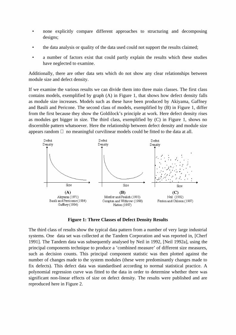
If we examine the various results we can divide them into three main classes. The first classcontains models, exemplified by graph (A) in Figure 1, that shows how defect density fallsas module size increases. Models such as these have been produced by Akiyama, Gaffneyand Basili and Pericone. The second class of models, exemplified by (B) in Figure 1, differfrom the first because they show the Goldilock’s principle at work. Here defect density risesas modules get bigger in size. The third class, exemplified by (C) in Figure 1, shows nodiscernible pattern whatsoever. Here the relationship between defect density and module sizeappears random no meaningful curvilinear models could be fitted to the data at all.

Figure 1: Three Classes of Defect Density Results

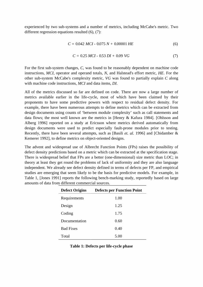
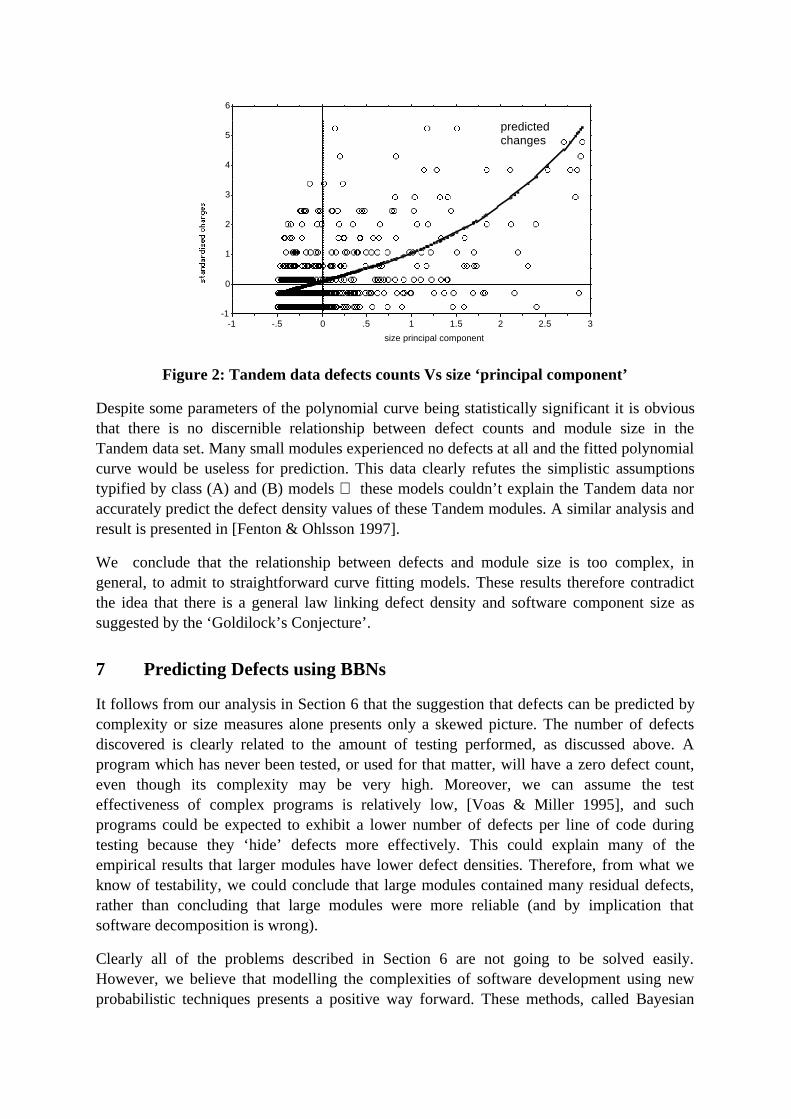
The third class of results show the typical data pattern from a number of very large industrialsystems. One data set was collected at the Tandem Corporation and was reported in, [Cherf1991]. The Tandem data was subsequently analysed by Neil in 1992, [Neil 1992a], using theprincipal components technique to produce a ’combined measure’ of different size measures,such as decision counts. This principal component statistic was then plotted against thenumber of changes made to the system modules (these were predominantly changes made tofix defects). This defect data was standardised according to normal statistical practice. Apolynomial regression curve was fitted to the data in order to determine whether there wassignificant non-linear effects of size on defect density. The results were published and arereproduced here in Figure 2.

-1

0

1

2

3

4

5

6

-1 -.5 0 .5 1 1.5 2 2.5 3

size principal component

predicted changes

Figure 2: Tandem data defects counts Vs size ‘principal component’

Despite some parameters of the polynomial curve being statistically significant it is obviousthat there is no discernible relationship between defect counts and module size in theTandem data set. Many small modules experienced no defects at all and the fitted polynomialcurve would be useless for prediction. This data clearly refutes the simplistic assumptionstypified by class (A) and (B) models these models couldn’t explain the Tandem data noraccurately predict the defect density values of these Tandem modules. A similar analysis andresult is presented in [Fenton & Ohlsson 1997].

We conclude that the relationship between defects and module size is too complex, ingeneral, to admit to straightforward curve fitting models. These results therefore contradictthe idea that there is a general law linking defect density and software component size assuggested by the ‘Goldilock’s Conjecture’.

7 Predicting Defects using BBNs

It follows from our analysis in Section 6 that the suggestion that defects can be predicted bycomplexity or size measures alone presents only a skewed picture. The number of defectsdiscovered is clearly related to the amount of testing performed, as discussed above. Aprogram which has never been tested, or used for that matter, will have a zero defect count,even though its complexity may be very high. Moreover, we can assume the testeffectiveness of complex programs is relatively low, [Voas & Miller 1995], and suchprograms could be expected to exhibit a lower number of defects per line of code duringtesting because they ‘hide’ defects more effectively. This could explain many of theempirical results that larger modules have lower defect densities. Therefore, from what weknow of testability, we could conclude that large modules contained many residual defects,rather than concluding that large modules were more reliable (and by implication thatsoftware decomposition is wrong).

Clearly all of the problems described in Section 6 are not going to be solved easily.However, we believe that modelling the complexities of software development using newprobabilistic techniques presents a positive way forward. These methods, called Bayesian

Belief Networks (BBNs), allow us to express complex inter-relations within the model at alevel of uncertainty commensurate with the problem. In this section we first provide anoverview of BBNs (Section 7.1) and describe the motivation for the particular BBN exampleused in defects prediction (Section 7.2). In Section 7.3 we describe the actual BBN.

7.1 An overview of BBNs

Bayesian Belief Networks (also known as Belief Networks, Causal Probabilistic Networks,Causal Nets, Graphical Probability Networks, Probabilistic Cause-Effect Models, andProbabilistic Influence Diagrams) have attracted much recent attention as a possible solutionfor the problems of decision support under uncertainty. Although the underlying theory(Bayesian probability) has been around for a long time, the possibility of building andexecuting realistic models has only been made possible because of recent algorithms andsoftware tools that implement them [Lauritzen & Spiegelhalter 1988]. To date BBNs haveproven useful in practical applications such as medical diagnosis and diagnosis ofmechanical failures. Their most celebrated recent use has been by Microsoft where BBNsunderlie the help wizards in Microsoft Office; also the ‘intelligent’ printer fault diagnosticsystem which you can run when you log onto Microsoft’s web site is in fact a BBN which, asa result of the problem symptoms you enter, identifies the most likely fault.

A BBN is a graphical network that represents probabilistic relationships among variables.BBNs enable reasoning under uncertainty and combine the advantages of an intuitive visualrepresentation with a sound mathematical basis in Bayesian probability. With BBNs, it ispossible to articulate expert beliefs about the dependencies between different variables and topropagate consistently the impact of evidence on the probabilities of uncertain outcomes,such as ‘future system reliability’. BBNs allow an injection of scientific rigour when theprobability distributions associated with individual nodes are simply ‘expert opinions’.

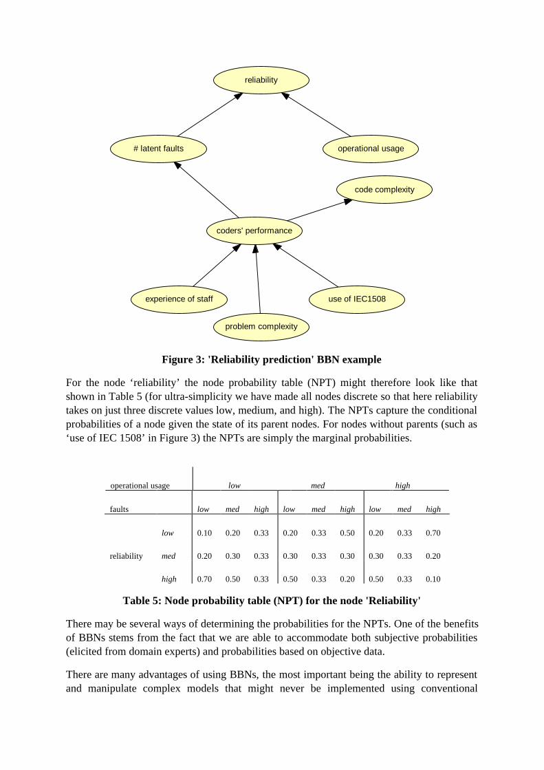
A BBN is a special type of diagram (called a graph) together with an associated set ofprobability tables. The graph is made up of nodes and arcs where the nodes representuncertain variables and the arcs the causal/relevance relationships between the variables.Figure 3 shows a BBN for an example ‘reliability prediction’ problem. The nodes representdiscrete or continuous variables, for example, the node ‘use of IEC 1508’ (the standard) isdiscrete having two values ‘yes’ and ‘no’, whereas the node ‘reliability’ might be continuous(such as the probability of failure). The arcs represent causal/influential relationshipsbetween variables. For example, software reliability is defined by the number of (latent)faults and the operational usage (frequency with which faults may be triggered). Hence wemodel this relationship by drawing arcs from the nodes ‘number of latent faults and‘operational usage’ to ‘reliability’.

experience of staff

problem complexity

use of IEC1508

# latent faults

code complexity

coders' performance

reliability

operational usage

Figure 3: 'Reliability prediction' BBN example

For the node ‘reliability’ the node probability table (NPT) might therefore look like thatshown in Table 5 (for ultra-simplicity we have made all nodes discrete so that here reliabilitytakes on just three discrete values low, medium, and high). The NPTs capture the conditionalprobabilities of a node given the state of its parent nodes. For nodes without parents (such as‘use of IEC 1508’ in Figure 3) the NPTs are simply the marginal probabilities.

operational usage low med high

faults low med high low med high low med high

low 0.10 0.20 0.33 0.20 0.33 0.50 0.20 0.33 0.70

reliability med 0.20 0.30 0.33 0.30 0.33 0.30 0.30 0.33 0.20

high 0.70 0.50 0.33 0.50 0.33 0.20 0.50 0.33 0.10

Table 5: Node probability table (NPT) for the node 'Reliability'

There may be several ways of determining the probabilities for the NPTs. One of the benefitsof BBNs stems from the fact that we are able to accommodate both subjective probabilities(elicited from domain experts) and probabilities based on objective data.

There are many advantages of using BBNs, the most important being the ability to representand manipulate complex models that might never be implemented using conventional

methods. Another advantage is that the model can predict events based on partial oruncertain data. Because BBNs have a rigorous, mathematical meaning there are softwaretools that can interpret them and perform the complex calculations needed in their use[HUGIN 1998].

The benefits of using BBNs include:

• specification of complex relationships using conditional probability statements;

• use of ‘what-if?’ analysis and forecasting of effects of process changes;

• easier understanding of chains of complex and seemingly contradictory reasoning viathe graphical format;

• explicit modelling of ‘ignorance’ and uncertainty in estimates;

• use of subjectively or objectively derived probability distributions;

• forecasting with missing data.

7.2 Motivation for BBN approach

Clearly defects are not directly caused by program complexity alone. In reality thepropensity to introduce defects will be influenced by many factors unrelated to code ordesign complexity. There are a number of causal factors at play when we want to explain thepresence of defects in a program:

• Difficulty of the problem

• Complexity of designed solution

• Programmer/Analyst skill

• Design methods and procedures used

Eliciting requirements is a notoriously difficult process and is widely recognised as beingerror prone. Defects introduced at the requirements stage are claimed to be the mostexpensive to remedy if they are not discovered early enough. Difficulty depends on theindividual trying to understand and describe the nature of the problem as well as the problemitself. A ‘sorting’ problem may appear difficult to a novice programmer but not to an expert.It also seems that the difficulty of the problem is partly influenced by the number of failedattempts at solutions there have been and whether a ‘ready made’ solution can be reused.Thus, novel problems have the highest potential to be difficult and ‘known’ problems tend tobe simple because known solutions can be identified and reused. Any software developmentproject will have a mix of ‘simple’ and ‘difficult’ problems depending on what intellectualresources are available to tackle them. Good managers know this and attempt to preventdefects by pairing up people and problems; easier problems to novices and difficult problemsto experts.

When assessing a defect it is useful to determine when it was introduced. Broadly speaking

there are two types of defect; those that are introduced in the requirements and thoseintroduced during design (including coding/implementation which can be treated as design).Useful defect models need to explain why a module has a high or low defect count if we areto learn from its use, otherwise we could never intervene and improve matters. Models usingsize and complexity metrics are structurally limited to assuming that defects are solelycaused by the internal organisation of the software design. They cannot explain defectsintroduced because:

• the ‘problem’ is ‘hard’;

• problem descriptions are inconsistent;

• the wrong ‘solution’ is chosen and does not fulfil the requirements.

We have long recognised in software engineering that program quality can be potentiallyimproved through the use of proper project procedures and good design methods. Basicproject procedures like configuration management, incident logging, documentation andstandards should help reduce the likelihood of defects. Such practices may not help theunique genius you need to work on the really difficult problems but they should raise thestandards of the mediocre.

Central to software design method is the notion that problems and designs can bedecomposed into meaningful chunks where each can be readily understood alone and finallyrecomposed to form the final system. Loose coupling between design components issupposed to help ensure that defects are localised and that consistency is maintained. Whatwe have lacked as a community is a theory of program composition and decomposition,instead we have fairly ill-defined ideas on coupling, modularity and cohesiveness. Howeverdespite not having such a theory every day experience tells us that these ideas help reducedefects and improve comprehension. It is indeed hard to think of any other scientific orengineering discipline that has not benefited from this approach.

Surprisingly, much of the defect prediction work has been pursued without reference totesting or testability. According to [Voas & Miller 1995, Bertolino & Strigini 1996] thetestability of a program will dictate its propensity to reveal failures under test conditions anduse. Also, at a superficial level the amount of testing performed will determine how manydefects will be discovered, assuming there are defects there to discover. Clearly, if no testingis done then no defects will be found. By extension we might argue that difficult problems,with complex solutions, might be difficult to test and so might demand more test effort. Ifsuch testing effort is not forthcoming (as is typical in many commercial projects whendeadlines loom) then less defects will be discovered, thus giving an over estimate of thequality achieved and a false sense of security. Thus, any model to predict defects mustinclude testing and testability as crucial factors.

7.3 A prototype BBN

Whilst there is insufficient space here to fully describe the development and execution of aBBN model here we have developed a prototype BBN to show the potential of BBNs andillustrate their useful properties. This prototype does not exhaustively model all of the issues

described in Section 7.2 nor does it solve all of the problems described in Section 6. Rather,it shows the possibility of combining the different software engineering schools of thoughton defect prediction into a single model. With this model we should be able to show howpredictions might be made and explain historical results more clearly.

The majority of the nodes have the following states: ‘very-high’, ‘high’, ‘medium’, ‘low’,‘very low’, except for the design size node and defect count nodes which have integer valuesor ranges and the defect density nodes which have real values. The probabilities attached toeach of these states are fictitious but are determined from an analysis of the literature orcommon-sense assumptions about the direction and strength of relations between variables.

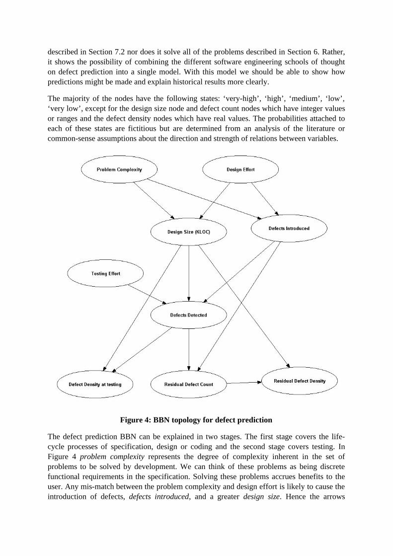
Figure 4: BBN topology for defect prediction

The defect prediction BBN can be explained in two stages. The first stage covers the life-cycle processes of specification, design or coding and the second stage covers testing. InFigure 4 problem complexity represents the degree of complexity inherent in the set ofproblems to be solved by development. We can think of these problems as being discretefunctional requirements in the specification. Solving these problems accrues benefits to theuser. Any mis-match between the problem complexity and design effort is likely to cause theintroduction of defects, defects introduced, and a greater design size. Hence the arrows

between design effort, problem complexity, introduced defects and design size. The testingstage follows the design stage and in practice the testing effort actually allocated may bemuch less than that required. The mis-match between testing effort and design size willinfluence the number of defects detected, which is bounded by the number of defectsintroduced. The difference between the defects detected and defects introduced is theresidual defects count. The defect density at testing is a function of the design size anddefects detected (defects/size). Similarly, the residual defect density is residual defectsdivided by design size.

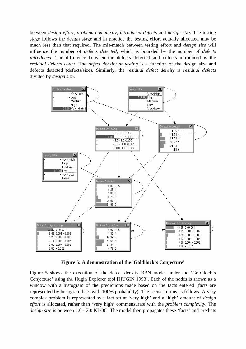
Figure 5: A demonstration of the 'Goldilock’s Conjecture'

Figure 5 shows the execution of the defect density BBN model under the ‘Goldilock’sConjecture’ using the Hugin Explorer tool [HUGIN 1998]. Each of the nodes is shown as awindow with a histogram of the predictions made based on the facts entered (facts arerepresented by histogram bars with 100% probability). The scenario runs as follows. A verycomplex problem is represented as a fact set at ‘very high’ and a ‘high’ amount of designeffort is allocated, rather than ‘very high’ commensurate with the problem complexity. Thedesign size is between 1.0 - 2.0 KLOC. The model then propagates these ‘facts’ and predicts

the introduced defects, detected defects and the defect density statistics. The distribution fordefects introduced peaks at two with 33% probability but, because less testing effort wasallocated than required, the distribution of defects detected peaks around zero withprobability 62%. The distribution for defect density at testing contrasts sharply with theresidual defect density distribution in that the defect density at testing appears veryfavourable. This is of course misleading because the residual defect density distributionshows a much higher probability of higher defect density levels.

From the model we can see a credible explanation for observing large ‘modules’ with lowerdefect densities. Under-allocation of design effort for complex problems results in moreintroduced defects and higher design size. Higher design size requires more testing effort,which if unavailable, leads to less defects being discovered than are actually there. Dividingthe small detected defect counts with large design size values will result in small defectdensities at the testing stage. The model explains the ‘Goldilock’s Conjecture’ without ad-hoc explanation or identification of outliers.

Clearly the ability to use BBNs to predict defects will depend largely on the stability andmaturity of the development processes. Organisations that do not collect metrics data, do notfollow defined life-cycles or do not perform any forms of systematic testing will never beable to build or apply such models. This does not mean to say that less mature organisationscannot build reliable software, rather it implies that they cannot do so predictably andcontrollably. Achieving predictability of output, for any process, demands a degree ofstability rare in software development organisations. Similarly, replication of experimentalresults can only be predicated on software processes that are defined and repeatable. Thisclearly implies some notion of Statistical Process Control (SPC) for software development.

8 Conclusions

Much of the published empirical work in the defect prediction area is well in advance of theunfounded rhetoric sadly typical of much of what passes for software engineering research.However every discipline must learn as much, if not more, from its failures as its successes.In this spirit we have reviewed the literature critically with a view to better understand pastfailures and outline possible avenues for future success.

Our critical review of state-of-the-art of models for predicting software defects has shownthat many methodological and theoretical mistakes have been made. Many past studies havesuffered from a variety of flaws ranging from model mis-specification to use ofinappropriate data. The issues and problems surrounding the ‘Goldilock’s Conjecture’illustrate how difficult defect prediction is and how easy it is to commit serious modellingmistakes. Specifically, we conclude that the existing models are incapable of predictingdefects accurately using size and complexity metrics alone. Furthermore, these models offerno coherent explanation of how defect introduction and detection variables affect defectcounts. Likewise any conclusions that large modules are more reliable and that softwaredecomposition doesn’t work are premature.

Each of the different ‘schools of thought’ have their own view of the prediction problemdespite the interactions and subtle overlaps between process and product identified here.

Furthermore each of these views model a part of the problem rather than the whole. Perhapsthe most critical issue in any scientific endeavour is agreement on the constituent elements orvariables of the problem under study. Models are developed to represent the salient featuresof the problem in a systemic fashion. This is as much the case in physical sciences as socialsciences. Economists could not predict the behaviour of an economy without an integrated,complex, macro-economic model of all of the known, pertinent variables. Excluding keyvariables such as savings rate or productivity would make the whole exercise invalid. Bytaking the wider view we can construct a more accurate picture and explain supposedlypuzzling and contradictory results. Our analysis of the studies surrounding the ‘Goldilock’sConjecture’ shows how empirical results about defect density can make sense if we look foralternative explanations.

Collecting data from case studies and subjecting it to isolated analysis is not enough becausestatistics on its own does not provide scientific explanations. We need compelling andsophisticated theories that have the power to explain the empirical observations. The isolatedpursuit of these single issue perspectives on the quality prediction problem are, in the longer-term, fruitless. Part of the solution to many of the difficulties presented above is to developprediction models that unify the key elements from the diverse software quality predictionmodels. We need models that predict software quality by taking into account informationfrom the development process, problem complexity, defect detection processes and designcomplexity. We must understand the cause and effect relations between important variablesin order to explain why certain design processes are more successful than others in terms ofthe products they produce.

It seems that successful engineers already operate in a way that tacitly acknowledges thesecause-effect relations. After all if they didn’t how else could they control and deliver qualityproducts? Project managers make decisions about software quality using best guesses; itseems to us that will always be the case and the best that researchers can do is a) recognisethis fact and b) improve the ‘guessing’ process. We therefore need to model the subjectivityand uncertainty that is pervasive in software development. Likewise, the challenge forresearchers is in transforming this uncertain knowledge, which is already evident in elementsof the various quality models already discussed, into a prediction model that other engineerscan learn from and apply. We are already working on a number of projects using BayesianBelief Networks as a method for creating more sophisticated models for prediction, [Neil &Fenton 1996, Neil et. al. 1996], and have described one of the prototype BBNs to outline theapproach. Ultimately, this research is aiming to produce a method for the statistical processcontrol (SPC) of software production implied by the SEI’s Capability Maturity Model.

All of the defect prediction models reviewed in this paper operate without the use of anyformal theory of program/problem decomposition. The literature is however replete withacknowledgements to cognitive explanations of shortcomings in human informationprocessing. While providing useful explanations of why designers employ decomposition asa design tactic they do not, and perhaps cannot, allow us to determine objectively theoptimum level of decomposition within a system (be it a requirements specification or a

program). The literature recognises the two structural3 aspects of software, ‘within’component structural complexity and ‘between’ component structural complexity, but welack the way to crucially integrate these two views in a way that would allow us to saywhether one design was more or less structurally complex than another. Such a theory mightalso allow us to compare different decompositions of the same solution to the same problemrequirement, thus explaining why different approaches to problem or design decompositionmight have caused a designer to commit more or less defects. As things currently standwithout such a theory we cannot compare different decompositions and therefore cannotcarry out experiments comparing different decomposition tactics. This leaves a gap in anyevolving science of software engineering that cannot be bridged using current case studybased approaches, despite their empirical flavour.

Acknowledgements

The work carried out here was partly funded by the ESPRIT projects SERENE and DeVa,the EPSRC project IMPRESS and the DISPO project funded by Scottish Nuclear. Theauthors are indebted to Niclas Ohlsson and Peter Popov for comments that have influencedthis work and the anonymous reviewers for their helpful and incisive contributions.

References

[Adams 1984] Adams, E., Optimizing preventive service of software products, IBMResearch Journal, 28(1), pp.2-14, 1984.

[Akiyama 1971] Akiyama, F., An example of software system debugging, Inf Processing71, pp.353-379, 1971.

[Bache & Bazzana 1993] Bache, R. and Bazzana, G. Software metrics for productassessment , McGraw Hill, London, 1993.

[Basili et. al. 1996] Basili, V., Briand L. and Melo W.L., A validation of object orienteddesign metrics as quality indicators, IEEE Transactions on Software Engineering, 1996.

[Basili & Perricone 1984] Basili, V.R. and Perricone B.T., Software Errors and Complexity:An Empirical Investigation, Communications of the ACM, 1984, pp.42-52.

[Bertolino & Strigini 1996] Bertolino, A. and Strigini, L., On the use of testability measuresfor dependability assessment, IEEE Transactions on Software Engineering 22(2), pp.97-108,1996.

[Brocklehurst & Littlewood 1992] Brocklehurst, S. and Littlewood B., New ways to getaccurate software reliability modelling, IEEE Software, July, 1992.

3 We are careful here to use the term structural complexity when discussing attributes of design artefacts

and cognitive complexity when referring to an individuals understanding of such an artefact. Suffice

it to say that structural complexity would influence cognitive complexity.

[Buck & Robbins 1984] Buck, R.D. and Robbins, J.H., Application of software inspectionmethodology in design and code, in Software Validation (Ed. H-L Hausen), ElsevierScience, 1984, pp.41-56.

[Cherf 1991] Cherf, S., An investigation of the maintenance and support characteristics ofcommercial software. Proceedings of the 2nd Oregon Workshop on Software Metrics(AOWSM), Portland, USA, 1991.

[Chidamber & Kemerer 1994] Chidamber, S.R. and Kemerer, C.F., A metrics suite forobject oriented design, IEEE Trans Software Eng, 20 (6), pp.476-498, 1994.

[Compton & Withrow 1990] Compton, T. and Withrow, C., Prediction and control of Adasoftware defects, J Systems Software, 12, pp.199-207, 1990.

[Cusumano 1991] Cusumano, M.A., Japan's Software Factories, Oxford University Press,1991.

[Diaz & Sligo 1997] M. Diaz and J. Sligo, How software process improvement helpedMotorola, IEEE Software, Vol.14, No.5, pp.75-81, 1997.

[Dyer 1992] Dyer, M., The Cleanroom approach to quality software development, Wiley,1992.

[Fenton 1994] Fenton, N.E., Software measurement: a necessary scientific basis, IEEETrans Software Eng 20 (3), pp.199-206, 1994.

[Fenton et. al. 1994] Fenton, N.E. and Pfleeger, S.L., Glass R, Science and Substance: AChallenge to Software Engineers, IEEE Software, July 1994, pp.86-95

[Fenton & Kitchenham 1991] Fenton N.E. and Kitchenham B.A., Validating softwaremeasures, J Software Testing, Verification & Reliability 1(2), 1991, pp.27-42

[Fenton & Ohlsson 1997] Fenton, N. and Ohlsson N., Quantitative Analysis of Faults andFailures in a Complex Software System. Submitted to IEEE Trans. Soft. Eng. June 1997.

[Fenton & Pfleeger 1996] Fenton, N.E. and Pfleeger, S.L., Software Metrics: A Rigorousand Practical Approach, (2nd Edition), International Thomson Computer Press, 1996.

[Ferdinand 1974] A.E. Ferdinand, A theory of system complexity. Int. J. General Syst.Vol.1, pp.19-33, 1974

[Gaffney 1984] Gaffney, J.R., Estimating the Number of Faults in Code, IEEE Trans.Software Engineering, Vol.SE-10, No.4, 1984

[Grady 1992] Grady, R.B. Practical Software Metrics for Project Management and ProcessImprovement. Prentice-Hall, 1992.

[Halstead 1975] Halstead, M.H. Elements of Software Science. Elsevier North-Holland,1975.

[Hamer & Frewin 1982] Hamer P, Frewin G, Halstead’s software science: a criticalexamination, Proc 6th Int Conf Software Eng, pp.197-206, 1982

[Hatton 1993] Hatton, L., The automation of software process and product quality. In M.Ross, C. A. Brebbia, G. Staples, & J. Stapleton (Eds.), Software Quality Management, (pp.727-744). Southampton: Computation Mechanics Publications, Elsevier 1993.

[Hatton 1994] Hatton, L. C., Safety Related Software Development: Standards, Subsets,testing, Metrics, Legal issues. McGraw-Hill, 1994.

[Hatton 1997] Hatton, L., Re-examining the Fault Density-Component Size Connection.IEEE Software, March/April 1997, Vol. 14 No. 2, pp.89-98.

[Henry & Kafura 1981] Henry, S. and Kafura, D., Software structure metrics based oninformation flow, IEEE Transaction on Software Engineering, 9,81, pp.510-518.

[Henry & Kafura 1984] Henry, S. and Kafura, D., The evaluation of software system'sstructure using quantitative software metrics, Software - Practice and Experience 14(6),pp.561-573 (June 1984).

[HUGIN 1998] HUGIN Expert Brochure, Hugin Expert A/S, P.O. Box 8201 DK-9220Aalborg, Denmark, 1998.

[Humphrey 1989] Humphrey, W. S., Managing the Software Process, Addison-Wesley,Reading, Massachusetts, 1989.

[Jones 1996] Jones, C., The Pragmatics of Software Process Improvements. In the ‘SoftwareEngineering Technical Council Newsletter’, Technical Council on Software Engineering,IEEE Computer Society, Winter 1996 - Vol. 14 No. 2.

[Jones 1991] Jones, C., Applied Software Measurement, McGraw Hill, 1991

[Keller 1992] Keller, T., Measurements role in providing “error-free” onboard shuttlesoftware, 3rd Intl Applications of Software Metrics Conference, La Jolla, California",pp.2.154-2.166, 1992, Proceedings available from Software Quality Engineering.

[Khoshgoftaar & Munson 1990] Khoshgoftaar, T.M. and Munson J.C., Predicting softwaredevelopment errors using complexity metrics, IEEE J of Selected Areas in Communications,8(2), pp.253-261, 1990

[Kitchenham 1988] Kitchenham, B.A., An evaluation of software structure metrics, Proc.COMPSAC 88, Chicago IL, USA, 1988.

[Kitchenham et. al. 1990] Kitchenham, B.A., Pickard, L.M. and Linkman, S.J., Anevaluation of some design metrics, Software Eng J, 5(1), 1990, pp.50-58.

[Koga 1992] Koga, K., Software Reliability Design Method in Hitachi, Proceedings of the3rd European Conference on Software Quality, Madrid, 1992

[Lauritzen & Spiegelhalter 1988] S.L. Lauritzen and D.J. Spiegelhalter, Local Computationswith Probabilities on Graphical Structures and their Application to Expert Systems (withdiscussion). J. R. Statis. Soc. Series B, 50, No 2, pp.157-224, 1988.

[Li & Henry 1993] Li, W. and Henry, S., Maintenance Metrics for the Object-OrientedParadigm. First International Software Metrics Symposium, May 21-22, 1993. BaltimoreMaryland IEEE Computer Society Press.

[Lipow 1982] Lipow, M., Number of Faults per Line of CODE, IEEE Trans. SoftwareEngineering, Vol.SE-8, No.4, 1982, pp.437-439, 1982

[Manly 1986] Manly, B. F., Multivariate Statistical methods: A Primer, Chapman and Hall,1986

[Moeller & and Paulish 1993] Moeller, K.H. and Paulish, D., An emprirical investigation ofsoftware fault distribution, Proc 1st Intl Software Metrics Symp, IEEE CS Press, pp.82-90,1993

[Munson & Khoshgoftaar 1990] Munson, J.C., and Khoshgoftaar, T.M., RegressionModelling of software quality: an empirical investigation, Inf. and Software Tech. 32(2),pp.106-114, 1990.

[Munson & Khoshgoftaar 1992] Munson, J.C., and Khoshgoftaar, T.M., The detection offault-prone programs, IEEE Trans. on Software Eng.18(5), pp.423-433, 1992

[Nakajo & Kume 1991] Nakajo, T. and Kume, H. A case History Analysis of SoftwareError Cause-Effect Relationships - IEEE Trans. on Software Eng. Vol 17 No.8 Aug.1991

[Neil & Fenton 1996] Neil, M. and Fenton N.E., Predicting software quality using Bayesianbelief networks, Proc 21st Annual Software Eng Workshop, NASA Goddard Space FlightCentre, pp.217-230, Dec, 1996.

[Neil et. al. 1996] Neil, M. Littlewood, B. and Fenton, N., Applying Bayesian BeliefNetworks to Systems Dependability Assessment. Proceedings of Safety Critical SystemsClub Symposium, Leeds, 6-8 February 1996. Published by Springer-Verlag.

[Neil 1992a] Neil, M.D., Multivariate Assessment of Software Products. Journal ofSoftware Testing, Verification and Reliability, Vol 1(4), pp.17-37, 1992.

[Neil 1992b] Neil, M.D. Statistical Modelling of Software Metrics. Ph.D. Thesis, SouthBank University and Strathclyde University, 1992.

[Ohlsson & Alberg 1996] Ohlsson, N. and Alberg, H., Predicting error-prone softwaremodules in telephone switches, IEEE Trans. on Software Eng., 22(12), pp.886-894, 1996.

[Ottenstein 1979] Ottenstein, L.M., Quantitative estimates of debugging requirements, IEEETrans. on Software Eng.5(5), pp.504-514, 1979

[Pfleeger & Fenton 1994] Pfleeger, S.L., Fenton, N.E. and Page S., Use of measurement inassessing standards and methods, IEEE Computer, Sept, 1994

[Potier et. al. 1982] Potier, D., Albin, J.L., Ferreol, R., Bilodeau, A., Experiments withcomputer software complexity and reliability, Proc 6th Intl Conf Software Eng, pp.94-103,1982

[Rosenberg 1997] J. Rosenberg, Some misconceptions about lines of code. Software MetricsSymposium, IEEE Comp Soc, pp.37-142, 1997.

[Schneidewind & Hoffmann 1979] Schneidewind, N.F. and Hoffmann, H., An experimentin Software Error data Collection and Analysis, IEEE Trans. on Software Eng. Vol 5 N.3May 1979

[Shen et. al. 1983] Shen, V.Y., Conte, S.D. and Dunsmore, H., Software science revisited: acritical analysis of the theory and its empirical support, IEEE Trans. on Software Eng.,SE-9(2), 1983, pp.155-165.

[Shen et. al. 1985] Shen, V.Y., Yu, T., Thebaut, S.M. and Paulsen, L.R., Identifyingerror-prone software - an empirical study, IEEE Trans. on Software Eng. Vol. 11(4) 1985,pp.317-323.

[Shepperd 1988] Shepperd, M.J., A critique of cyclomatic complexity as a softwaremetric, Softw. Eng. J. vol 3 No 2 (1988) pp.30-36

[Shooman 1983] Shooman, M.L., Software Engineering : Design, Reliability andManagement, McGraw-Hill, 1983.

[Stalhane 1992] Stalhane, T., Practical Experiences with Safety Assessment of a System forAutomatic Train Control Proceedings of SAFECOMP’92, Zurich, Switzerland. Published byPergamon Press in Oxford, UK, 1992.

[Veevers & Marshall 1994] Veevers, A. and Marshall, A.C., A relationship betwen softwarecoverage metrics and reliability', J Software Testing, Verification and Reliability, 4, pp.3-8,1994

[Voas et. al. 1995] Voas J., Michael C. and Miller K. Confidently Assessing a ZeroProbability of Software Failure, High Integrity Systems, Vol 1 No. 3, 1995, pp.269-275.

[Voas & Miller 1995] Voas, J.M. and Miller, K.W., Software testability: the newverfication, IEEE Software, pp.17-28, May, 1995.

[Yasuda 1989] Yasuda, K. Software Quality Assurance Activities in Japan. In JapanesePerspectives in Software Engineering,.187-205, Addison-Wesley, 1989.

[Zhou et. al. 1993] Zhou, F., Lowther, B., Oman, P. and Hagemeister, J., Constructing andTesting Software Maintainability Assessment Models, May 21-22, 1993. BaltimoreMaryland. IEEE Computer Society Press.