Defect Prediction Model for estimating Project Scheduleuploads.pnsqc.org/2016/papers/45.DefectPrediction... · Defect Prediction Model for estimating Project Schedule Rajesh Yawantikar,

Excerpt from PNSQC 2016 Proceedings PNSQC.ORG Copies may not be made or distributed for commercial use Page 1

Defect Prediction Model for estimating Project Schedule

Rajesh Yawantikar, Debashish Barua, Anupriya Vatta

{rajesh.yawantikar, debashish.barua, anupriya.vatta}@intel.com

Abstract Many organizations want to estimate the number of defects prior to a product’s launch in order to estimate the product quality and maintenance effort. Another serious concern for the Project management is about defining the project milestone schedules. Some of problems that needs to be addressed are: What if Alpha, Beta, and Production Release milestones are planned way too early or too late? How does the number of open defects impact the program schedule? Are there any existing tools which can aid for scheduling project milestones (Alpha, Beta, and PRQ i.e. Product Release Qualification)?

This paper addresses the above problems and we demonstrate this by applying our Defect Prediction Model in estimating project milestones. We’ll take a closer look at identifying the common mistakes made by the Project Management in declaring the milestones. Using this model, we can identify the risk in the existing program schedule. Additionally, we can monitor in-process quality of products and take preventive actions on the unforeseen defects/issues/risks. We have successfully applied our model to approximately 50 different platforms across different business segments and as a result taken preventive measures in upcoming projects and releasing the products on time.

Biography Rajesh Yawantikar is Senior Software Quality Manager at Intel Corporation, he is responsible for all aspects of software quality and reliability across mobility products this includes tablets and phones. With over all experience of 19+ years in software Quality, of which 10 years with Intel. Rajesh won 5 Intel Software Quality Awards (highest award in Software at Intel), now he mentors several teams for Intel Software Quality Award. Rajesh leads the external industry collaborations for Intel Software Quality group, this includes working with various industry bodies and academia. Rajesh is Board member of IEEE Computer Society- Professional Education and Activities Board.

Debashish Barua is a Software Quality Engineer at Intel. Debashish has a Master’s degree in Electrical and Computer Engineering from University of California, Santa Barbara. He is well versed with Statistical Analysis and Machine Learning and has over 4 years of work experience in the software industry.

Anupriya Vatta joined Intel as Software Quality Engineer 3 years ago with 5+ years of QA and automation experience, including companies like Blackberry, Ream Networks and Good etc. Anupriya has a Master’s degree in Computer Science from University of Texas at Dallas. As a SQE she is responsible for software initiatives and process improvements and helps multiple teams to adhere the best software practices. She is also always looking for innovative ideas and methodologies to improve the overall software lifecycle.


1 Introduction On one hand, we have to predict the number of Software Defects in an upcoming project. On the other hand, we need to schedule Project Milestones in such a way that the number of Defects are reduced with subsequent releases and thereby improving the quality of the product. There are many papers which predict Software defects using statistical models and metrics. The paper by Fenton and Neil (Fenton & Neil, 1999) critiqued on a wide range of Prediction Models. It covered complexity and size metrics, the testing process, the design and development process, and multivariate studies. Milestones are used in project management to mark specific points along a project timeline. These points may signal anchors such as a project start and end date, a need for external review or input and budget checks, among others. Project milestones focus on major progress points in the Product Life Cycle (PLC). We want to tackle these problems by correlating the number of Defects to the Project Milestones. With this in mind, we developed a Defect Prediction Model which integrates the Project Milestones and provides defects trends along with improved schedule for upcoming projects. In this paper, we cover Building a Prediction Model (Section 2), Defect Prediction Model using Logistic function (Section 3), Project Milestones (Section 4), Generate Reference Parameters from Past Projects (Section 5), and Predicting Defects and defining Project Milestones(Section 6).

2 Building a Prediction Model Our main objective is to build a model which is simple, easy to understand, and can be readily used by the Program / Project Managers. We have a huge database of defects containing historical data of previous projects. In our projects, we have used defect tracking systems like Jira (Jira Software, n.d.), Bugzilla (Bugzilla, n.d.), etc. to collect the defect data. At first, we plotted all the defects found in a project for the entire product lifecycle. These plots were random in nature, with many crests and troughs in the curve for different projects, making it difficult to perform analysis. In our next iteration, we chose to plot the Cumulative Defects instead of standalone ones. We observed a steady increasing trend for all the projects. In our third and final iteration, we chose to aggregate all the defects within a Work Week (5 business days from Monday to Friday) and plot the Cumulative Defects with respect to a Work Week (WW).

Figure 1: Plot of Cumulative Defects Vs WW for Project A

Figure 2: Plot of Cumulative Defects Vs WW for Project B

We observe an “S” shaped pattern for both the projects A and B. We decided to group the days into Work Weeks for the following reasons:


1. Agile based projects have typically 1 or 2 WWs as Sprints. Each sprint starts with a sprint planning event that aims to define a sprint backlog, identify the work for the sprint, and make an estimated commitment for the sprint goal.

2. Project Managers plan with respect to WWs. All the milestones are also defined in WW terminology.

Figure 1 and Figure 2 trends show that they follow the “S” trend. Figure 1 almost looks perfect whereas Figure 2 deviates a little but overall we can make a good assumption for an “S” curve. Also, we have highlighted the specific project milestones (Alpha, Beta, and PRQ) which will be discussed in detail in Project Milestones (Section 4). By carefully analyzing the defect trends of approximately 50 projects, we conclude that the projects when plotted by Cumulative Defects Vs WWs resemble the slanted version of the letter “S”.

2.1 The significance of S-curve in Project Management

Wideman (Wideman, May 2001) defined S-curve as follows: “A display of cumulative costs, labor hours or other quantities plotted against time. The name derives from the S-like shape of the curve, flatter at the beginning and end and steeper in the middle, which is typical of most projects. The beginning represents a slow, deliberate but accelerating start, while the end represents a deceleration as the work runs out.”

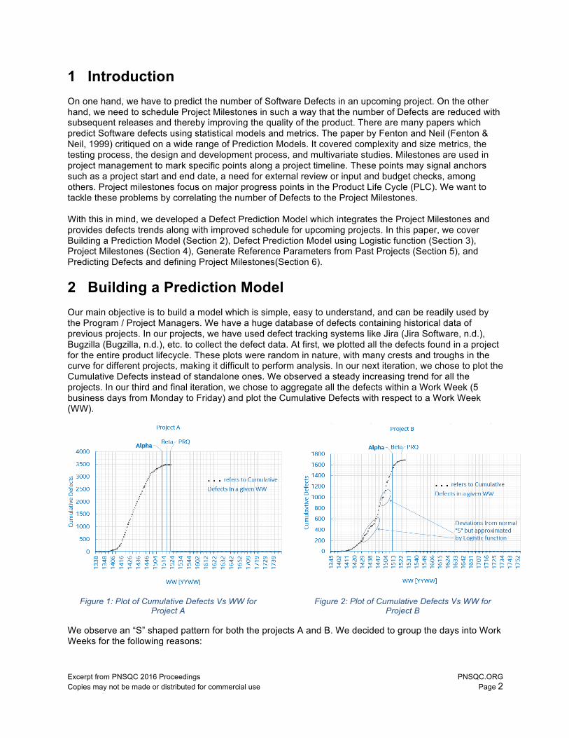
Garland’s (Garland, The Mysterious S-curve, 2009) article about the mysterious S-curves says, “S-curves are an important project management tool. They allow the progress of a project to be tracked visually over time, and form a historical record of what has happened till date. Analyses of S-curves allow project managers to quickly identify project growth, slippage, and potential problems that could adversely impact the project schedule if no remedial action is taken.” Figure 3, Figure 4, and Figure 5 are from (Garland, The Mysterious S-curve, 2009).

Figure 3: Project Growth

Figure 4: Project Slippage

Figure 5: Project Progress

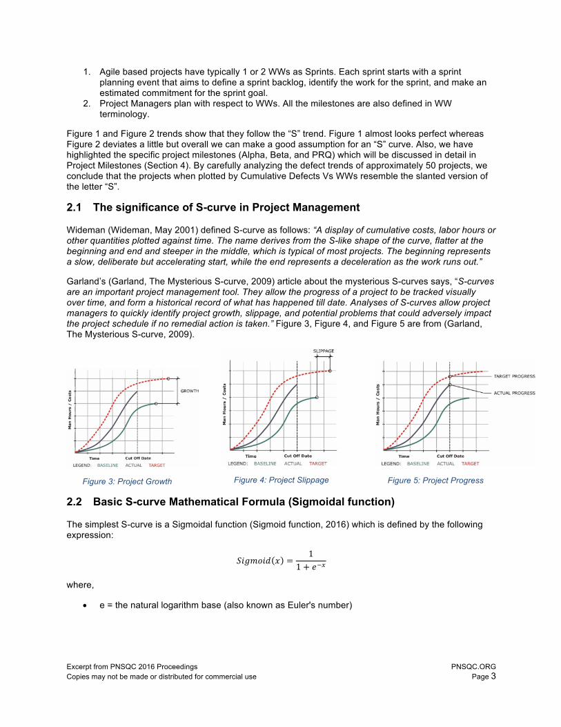
2.2 Basic S-curve Mathematical Formula (Sigmoidal function)

The simplest S-curve is a Sigmoidal function (Sigmoid function, 2016) which is defined by the following expression:

𝑆𝑆𝑆𝑆𝑆𝑆𝑆𝑆𝑆𝑆𝑆𝑆𝑆𝑆 𝑥𝑥 =1

1 + 𝑒𝑒,-

where,

• e = the natural logarithm base (also known as Euler's number)


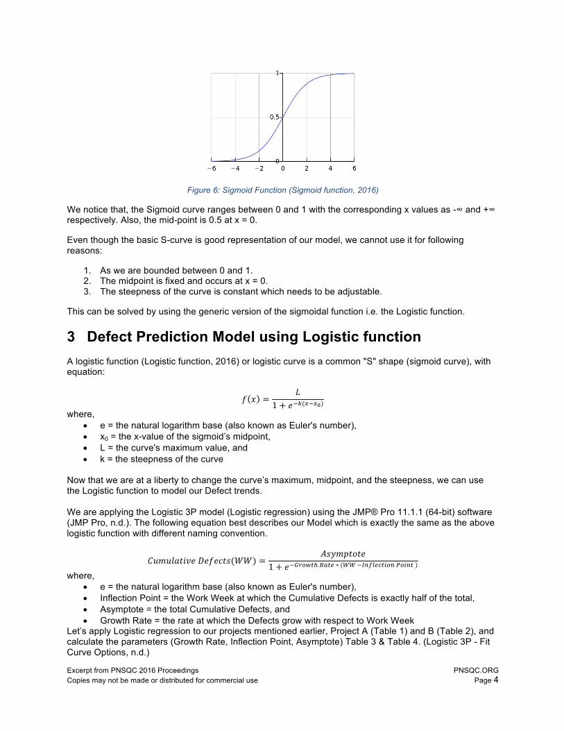
Figure 6: Sigmoid Function (Sigmoid function, 2016)

We notice that, the Sigmoid curve ranges between 0 and 1 with the corresponding x values as -∞ and +∞ respectively. Also, the mid-point is 0.5 at x = 0.

Even though the basic S-curve is good representation of our model, we cannot use it for following reasons:

1. As we are bounded between 0 and 1. 2. The midpoint is fixed and occurs at x = 0. 3. The steepness of the curve is constant which needs to be adjustable.

This can be solved by using the generic version of the sigmoidal function i.e. the Logistic function.

3 Defect Prediction Model using Logistic function A logistic function (Logistic function, 2016) or logistic curve is a common "S" shape (sigmoid curve), with equation:

𝑓𝑓 𝑥𝑥 =𝐿𝐿

1 + 𝑒𝑒,0(-,-2)

where, • e = the natural logarithm base (also known as Euler's number), • x0 = the x-value of the sigmoid’s midpoint, • L = the curve's maximum value, and • k = the steepness of the curve

Now that we are at a liberty to change the curve’s maximum, midpoint, and the steepness, we can use the Logistic function to model our Defect trends. We are applying the Logistic 3P model (Logistic regression) using the JMP® Pro 11.1.1 (64-bit) software (JMP Pro, n.d.). The following equation best describes our Model which is exactly the same as the above logistic function with different naming convention.

𝐶𝐶𝐶𝐶𝑆𝑆𝐶𝐶𝐶𝐶𝐶𝐶𝐶𝐶𝑆𝑆𝐶𝐶𝑒𝑒𝐷𝐷𝑒𝑒𝑓𝑓𝑒𝑒𝑒𝑒𝐶𝐶𝑒𝑒(𝑊𝑊𝑊𝑊) =𝐴𝐴𝑒𝑒𝐴𝐴𝑆𝑆𝐴𝐴𝐶𝐶𝑆𝑆𝐶𝐶𝑒𝑒

1 + 𝑒𝑒,BCDEFGHIFJ∗(LL,MNOPJQFRDNSDRNF)

where, • e = the natural logarithm base (also known as Euler's number), • Inflection Point = the Work Week at which the Cumulative Defects is exactly half of the total, • Asymptote = the total Cumulative Defects, and • Growth Rate = the rate at which the Defects grow with respect to Work Week

Let’s apply Logistic regression to our projects mentioned earlier, Project A (Table 1) and B (Table 2), and calculate the parameters (Growth Rate, Inflection Point, Asymptote) Table 3 & Table 4. (Logistic 3P - Fit Curve Options, n.d.)


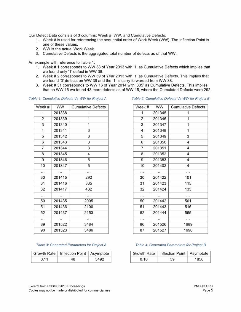
Our Defect Data consists of 3 columns: Week #, WW, and Cumulative Defects.

1. Week # is used for referencing the sequential order of Work Week (WW). The Inflection Point is one of these values.

2. WW is the actual Work Week 3. Cumulative Defects is the aggregated total number of defects as of that WW.

An example with reference to Table 1:

1. Week # 1 corresponds to WW 38 of Year 2013 with ‘1’ as Cumulative Defects which implies that we found only ‘1’ defect in WW 38.

2. Week # 2 corresponds to WW 39 of Year 2013 with ‘1’ as Cumulative Defects. This implies that we found ‘0’ defects on WW 39 and the ‘1’ is carry forwarded from WW 38.

3. Week # 31 corresponds to WW 16 of Year 2014 with ‘335’ as Cumulative Defects. This implies that on WW 16 we found 43 more defects as of WW 15, where the Cumulated Defects were 292.

Table 1: Cumulative Defects Vs WW for Project A

Week # WW Cumulative Defects 1 201338 1 2 201339 1 3 201340 1 4 201341 3 5 201342 3 6 201343 3 7 201344 3 8 201345 4 9 201346 5

10 201347 5 … … … 30 201415 292 31 201416 335 32 201417 432 … … … 50 201435 2005 51 201436 2100 52 201437 2153 … … … 89 201522 3484 90 201523 3486

Table 2: Cumulative Defects Vs WW for Project B

Week # WW Cumulative Defects 1 201345 1 2 201346 1 3 201347 1 4 201348 1 5 201349 3 6 201350 4 7 201351 4 8 201352 4 9 201353 4

10 201402 4 … … … 30 201422 101 31 201423 115 32 201424 135 … … … 50 201442 501 51 201443 516 52 201444 565 … … … 86 201526 1689 87 201527 1690

Table 3: Generated Parameters for Project A

Growth Rate Inflection Point Asymptote 0.11 48 3492

Table 4: Generated Parameters for Project B

Growth Rate Inflection Point Asymptote 0.10 59 1856


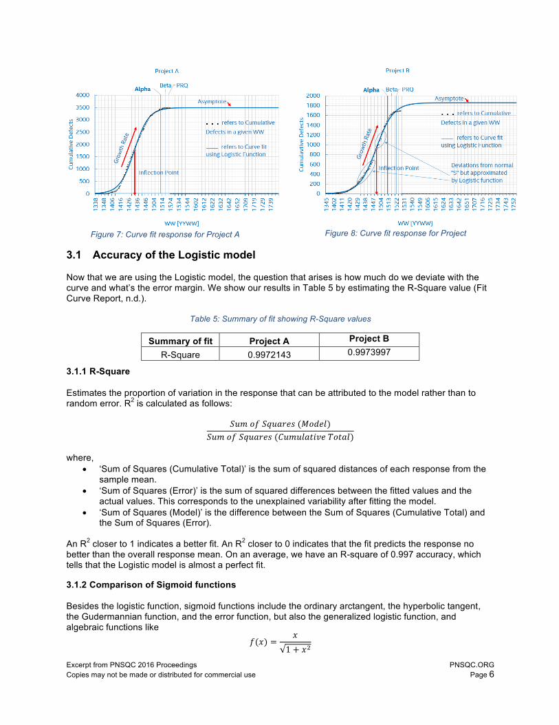
Figure 7: Curve fit response for Project A

Figure 8: Curve fit response for Project

3.1 Accuracy of the Logistic model

Now that we are using the Logistic model, the question that arises is how much do we deviate with the curve and what’s the error margin. We show our results in Table 5 by estimating the R-Square value (Fit Curve Report, n.d.).

Table 5: Summary of fit showing R-Square values

Summary of fit Project A Project B

R-Square 0.9972143 0.9973997

3.1.1 R-Square

Estimates the proportion of variation in the response that can be attributed to the model rather than to random error. R2 is calculated as follows:

𝑆𝑆𝐶𝐶𝑆𝑆𝑆𝑆𝑓𝑓𝑆𝑆𝑆𝑆𝐶𝐶𝐶𝐶𝑆𝑆𝑒𝑒𝑒𝑒(𝑀𝑀𝑆𝑆𝑆𝑆𝑒𝑒𝐶𝐶)𝑆𝑆𝐶𝐶𝑆𝑆𝑆𝑆𝑓𝑓𝑆𝑆𝑆𝑆𝐶𝐶𝐶𝐶𝑆𝑆𝑒𝑒𝑒𝑒(𝐶𝐶𝐶𝐶𝑆𝑆𝐶𝐶𝐶𝐶𝐶𝐶𝐶𝐶𝑆𝑆𝐶𝐶𝑒𝑒𝑇𝑇𝑆𝑆𝐶𝐶𝐶𝐶𝐶𝐶)

where,

• ‘Sum of Squares (Cumulative Total)’ is the sum of squared distances of each response from the sample mean.

• ‘Sum of Squares (Error)’ is the sum of squared differences between the fitted values and the actual values. This corresponds to the unexplained variability after fitting the model.

• ‘Sum of Squares (Model)’ is the difference between the Sum of Squares (Cumulative Total) and the Sum of Squares (Error).

An R2 closer to 1 indicates a better fit. An R2 closer to 0 indicates that the fit predicts the response no better than the overall response mean. On an average, we have an R-square of 0.997 accuracy, which tells that the Logistic model is almost a perfect fit.

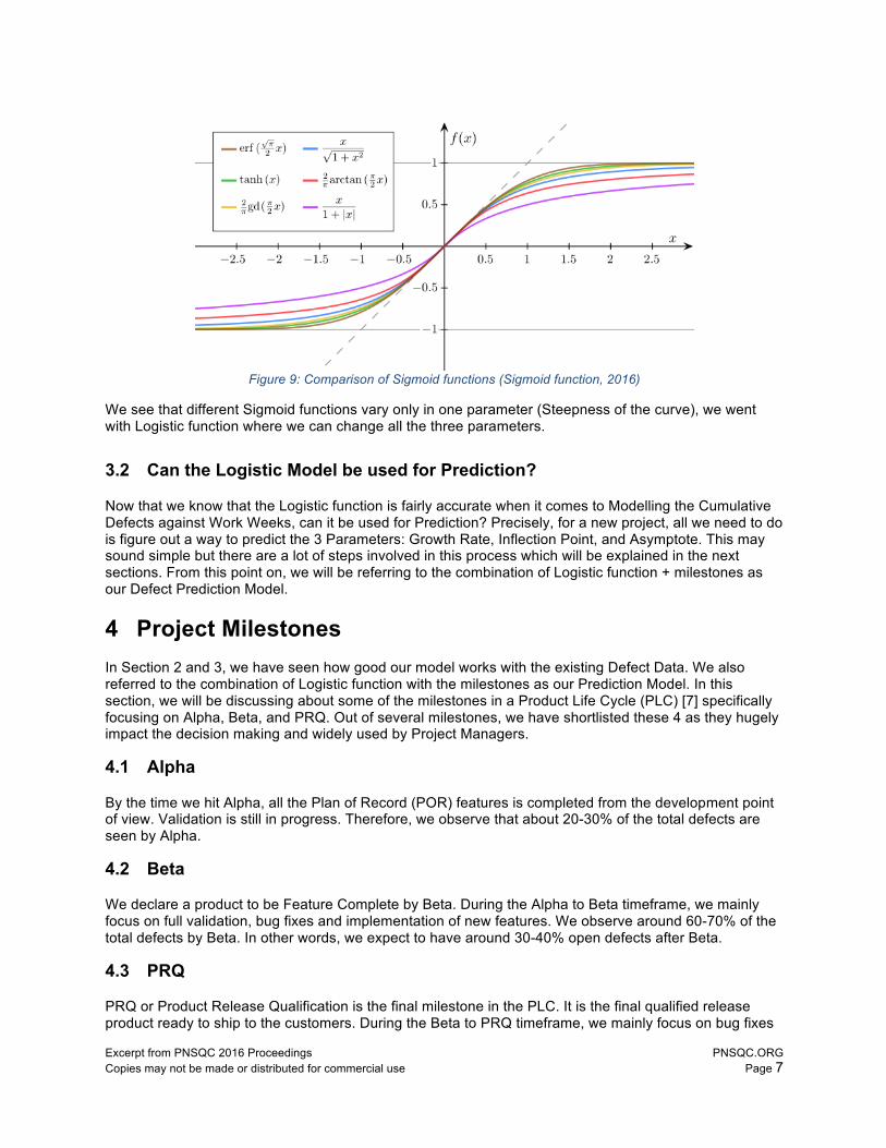
3.1.2 Comparison of Sigmoid functions

Besides the logistic function, sigmoid functions include the ordinary arctangent, the hyperbolic tangent, the Gudermannian function, and the error function, but also the generalized logistic function, and algebraic functions like

𝑓𝑓(𝑥𝑥) =𝑥𝑥

1 + 𝑥𝑥X


Figure 9: Comparison of Sigmoid functions (Sigmoid function, 2016)

We see that different Sigmoid functions vary only in one parameter (Steepness of the curve), we went with Logistic function where we can change all the three parameters.

3.2 Can the Logistic Model be used for Prediction?

Now that we know that the Logistic function is fairly accurate when it comes to Modelling the Cumulative Defects against Work Weeks, can it be used for Prediction? Precisely, for a new project, all we need to do is figure out a way to predict the 3 Parameters: Growth Rate, Inflection Point, and Asymptote. This may sound simple but there are a lot of steps involved in this process which will be explained in the next sections. From this point on, we will be referring to the combination of Logistic function + milestones as our Defect Prediction Model.

4 Project Milestones In Section 2 and 3, we have seen how good our model works with the existing Defect Data. We also referred to the combination of Logistic function with the milestones as our Prediction Model. In this section, we will be discussing about some of the milestones in a Product Life Cycle (PLC) [7] specifically focusing on Alpha, Beta, and PRQ. Out of several milestones, we have shortlisted these 4 as they hugely impact the decision making and widely used by Project Managers.

4.1 Alpha

By the time we hit Alpha, all the Plan of Record (POR) features is completed from the development point of view. Validation is still in progress. Therefore, we observe that about 20-30% of the total defects are seen by Alpha.

4.2 Beta

We declare a product to be Feature Complete by Beta. During the Alpha to Beta timeframe, we mainly focus on full validation, bug fixes and implementation of new features. We observe around 60-70% of the total defects by Beta. In other words, we expect to have around 30-40% open defects after Beta.

4.3 PRQ

PRQ or Product Release Qualification is the final milestone in the PLC. It is the final qualified release product ready to ship to the customers. During the Beta to PRQ timeframe, we mainly focus on bug fixes


and implement any new Change Request (CR) from customers. Beta and PRQ timelines could be very close to each other depending on the number of new requests. We observe that around 70-80% of the total defects by PRQ which leaves us to an estimated 20-30% open defects after PRQ.

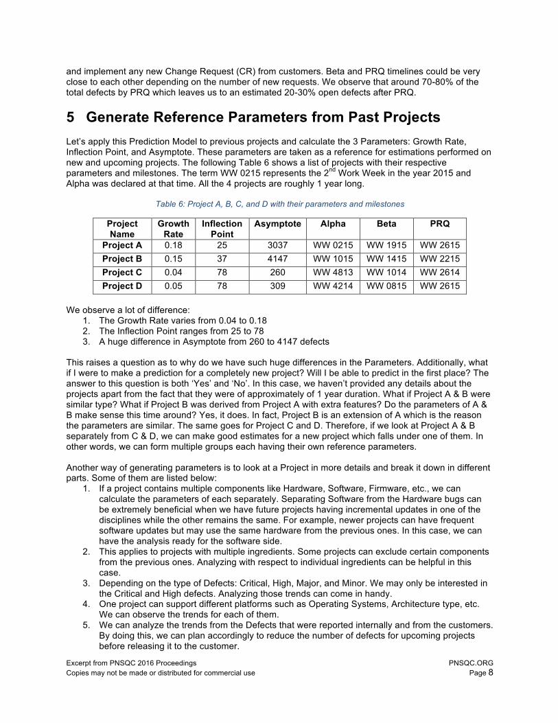
5 Generate Reference Parameters from Past Projects Let’s apply this Prediction Model to previous projects and calculate the 3 Parameters: Growth Rate, Inflection Point, and Asymptote. These parameters are taken as a reference for estimations performed on new and upcoming projects. The following Table 6 shows a list of projects with their respective parameters and milestones. The term WW 0215 represents the 2nd Work Week in the year 2015 and Alpha was declared at that time. All the 4 projects are roughly 1 year long.

Table 6: Project A, B, C, and D with their parameters and milestones

Project Name

Growth Rate

Inflection Point

Asymptote Alpha Beta PRQ

Project A 0.18 25 3037 WW 0215 WW 1915 WW 2615 Project B 0.15 37 4147 WW 1015 WW 1415 WW 2215 Project C 0.04 78 260 WW 4813 WW 1014 WW 2614 Project D 0.05 78 309 WW 4214 WW 0815 WW 2615

We observe a lot of difference:

1. The Growth Rate varies from 0.04 to 0.18 2. The Inflection Point ranges from 25 to 78 3. A huge difference in Asymptote from 260 to 4147 defects

This raises a question as to why do we have such huge differences in the Parameters. Additionally, what if I were to make a prediction for a completely new project? Will I be able to predict in the first place? The answer to this question is both ‘Yes’ and ‘No’. In this case, we haven’t provided any details about the projects apart from the fact that they were of approximately of 1 year duration. What if Project A & B were similar type? What if Project B was derived from Project A with extra features? Do the parameters of A & B make sense this time around? Yes, it does. In fact, Project B is an extension of A which is the reason the parameters are similar. The same goes for Project C and D. Therefore, if we look at Project A & B separately from C & D, we can make good estimates for a new project which falls under one of them. In other words, we can form multiple groups each having their own reference parameters. Another way of generating parameters is to look at a Project in more details and break it down in different parts. Some of them are listed below:

1. If a project contains multiple components like Hardware, Software, Firmware, etc., we can calculate the parameters of each separately. Separating Software from the Hardware bugs can be extremely beneficial when we have future projects having incremental updates in one of the disciplines while the other remains the same. For example, newer projects can have frequent software updates but may use the same hardware from the previous ones. In this case, we can have the analysis ready for the software side.

2. This applies to projects with multiple ingredients. Some projects can exclude certain components from the previous ones. Analyzing with respect to individual ingredients can be helpful in this case.

3. Depending on the type of Defects: Critical, High, Major, and Minor. We may only be interested in the Critical and High defects. Analyzing those trends can come in handy.

4. One project can support different platforms such as Operating Systems, Architecture type, etc. We can observe the trends for each of them.

5. We can analyze the trends from the Defects that were reported internally and from the customers. By doing this, we can plan accordingly to reduce the number of defects for upcoming projects before releasing it to the customer.


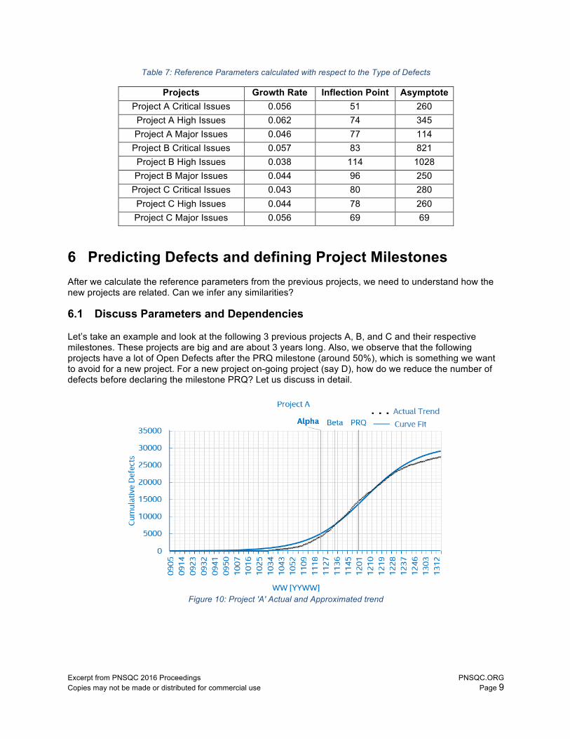
Table 7: Reference Parameters calculated with respect to the Type of Defects

Projects Growth Rate Inflection Point Asymptote Project A Critical Issues 0.056 51 260 Project A High Issues 0.062 74 345 Project A Major Issues 0.046 77 114

Project B Critical Issues 0.057 83 821 Project B High Issues 0.038 114 1028 Project B Major Issues 0.044 96 250

Project C Critical Issues 0.043 80 280 Project C High Issues 0.044 78 260 Project C Major Issues 0.056 69 69

6 Predicting Defects and defining Project Milestones After we calculate the reference parameters from the previous projects, we need to understand how the new projects are related. Can we infer any similarities?

6.1 Discuss Parameters and Dependencies

Let’s take an example and look at the following 3 previous projects A, B, and C and their respective milestones. These projects are big and are about 3 years long. Also, we observe that the following projects have a lot of Open Defects after the PRQ milestone (around 50%), which is something we want to avoid for a new project. For a new project on-going project (say D), how do we reduce the number of defects before declaring the milestone PRQ? Let us discuss in detail.

Figure 10: Project 'A' Actual and Approximated trend


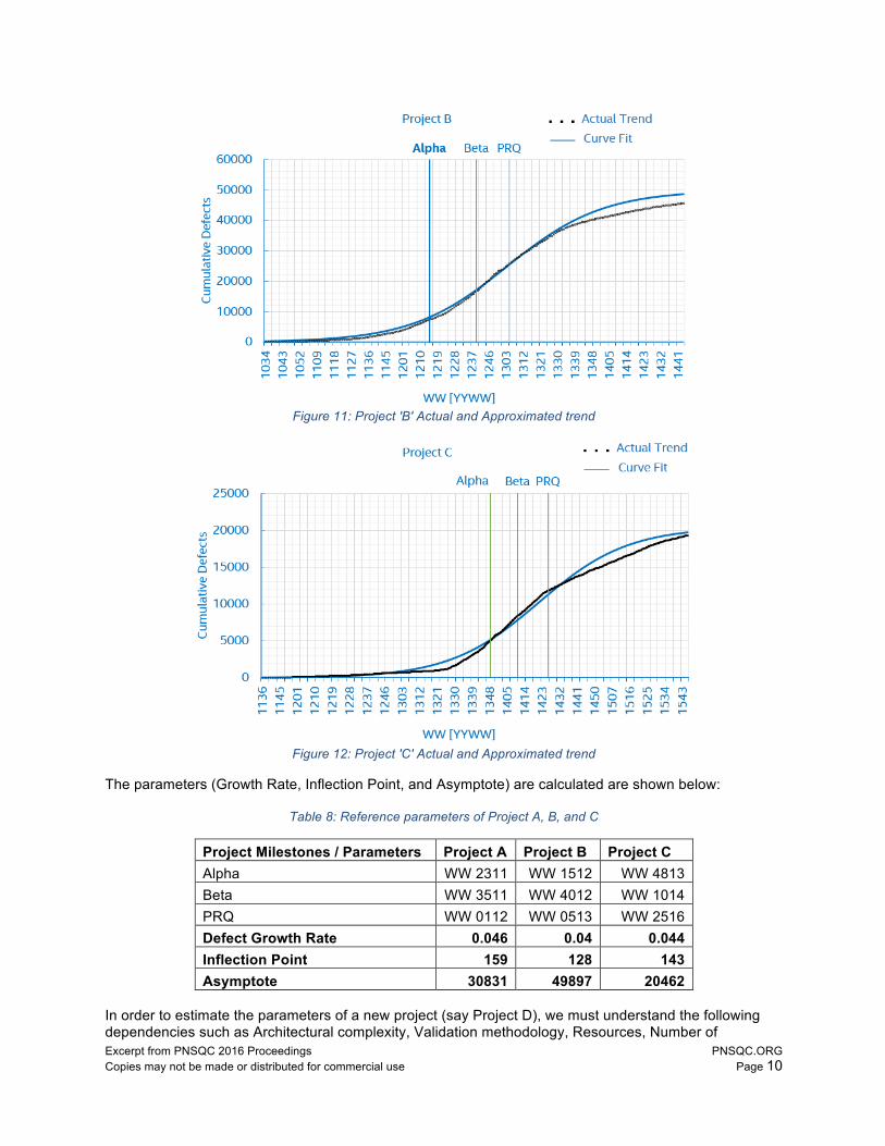
Figure 11: Project 'B' Actual and Approximated trend

Figure 12: Project 'C' Actual and Approximated trend

The parameters (Growth Rate, Inflection Point, and Asymptote) are calculated are shown below:

Table 8: Reference parameters of Project A, B, and C

Project Milestones / Parameters Project A Project B Project C Alpha WW 2311 WW 1512 WW 4813 Beta WW 3511 WW 4012 WW 1014 PRQ WW 0112 WW 0513 WW 2516 Defect Growth Rate 0.046 0.04 0.044 Inflection Point 159 128 143 Asymptote 30831 49897 20462

In order to estimate the parameters of a new project (say Project D), we must understand the following dependencies such as Architectural complexity, Validation methodology, Resources, Number of


Features, and Project Timelines. We will try to correlate the new Project D to any or all of the previous projects (A, B, C). We will perform Delta analysis between the previous projects and the new project. Also, note that we are not quantifying any of these dependencies. It is up to the user to make estimations based on their assumptions. Let’s take a look at few of the dependencies.

6.1.1 Architectural complexity

How complex is the architecture of Project A, B, and C? How are they different? Are they related? Is one the improvement of the other? Did we modify a particular architecture to a point that it is completely different? These questions need to be addressed by the Program Architects by looking at various platforms. We just assign the terms “Not Complex”, “Complex”, and “High Complexity” to those projects. Based on our observation, the complexity of a project is directly proportional to the Defect Growth Rate and Asymptote. This implies that, the higher complexity of the project, the more the Growth Rate as compared to the previous ones. In case of Inflection Point, we found that it is directly proportional to the Milestones but independent of the complexity.

6.1.2 More of Less Features

How many features were part of Project A, B, and C? Are some of the features similar to a new project? Are these features planned to be released for the first time? What about the number of programmers? Were there changes in Development methodology, Project culture, and development / verification technology? These questions need to be addressed by the Project Management for the previous projects. Based on our observations, the Number of Features in a project is directly proportional to all the 3 parameters: Defect Growth Rate, Inflection Point, and Asymptote. For example: A completely new feature never tested before will definitely increase the bug count.

6.1.3 Project Timelines

As timelines become cramped i.e. there isn’t much duration between any two milestones (Alpha – Beta, Beta – PRQ), we observe a lower Defect trend. As a result, we tend to miss out lot of defects before the final release (PRQ). In order to avoid this issue altogether, we need to have a significant duration between any two milestones. This will increase the bug count before the PRQ and we’ll see a higher Growth Rate and Asymptote.

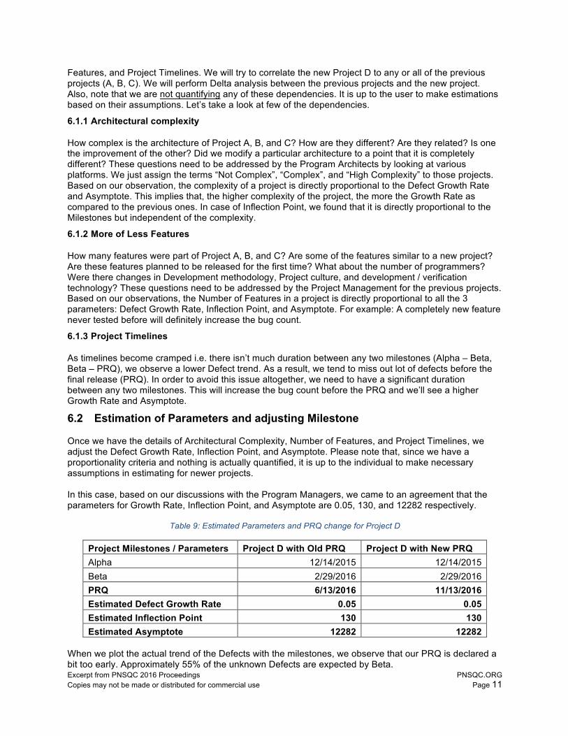
6.2 Estimation of Parameters and adjusting Milestone

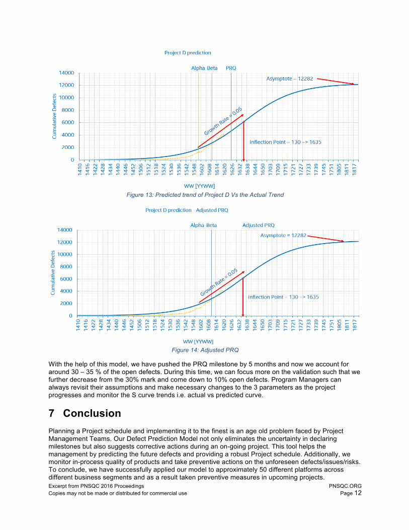
Once we have the details of Architectural Complexity, Number of Features, and Project Timelines, we adjust the Defect Growth Rate, Inflection Point, and Asymptote. Please note that, since we have a proportionality criteria and nothing is actually quantified, it is up to the individual to make necessary assumptions in estimating for newer projects. In this case, based on our discussions with the Program Managers, we came to an agreement that the parameters for Growth Rate, Inflection Point, and Asymptote are 0.05, 130, and 12282 respectively.

Table 9: Estimated Parameters and PRQ change for Project D

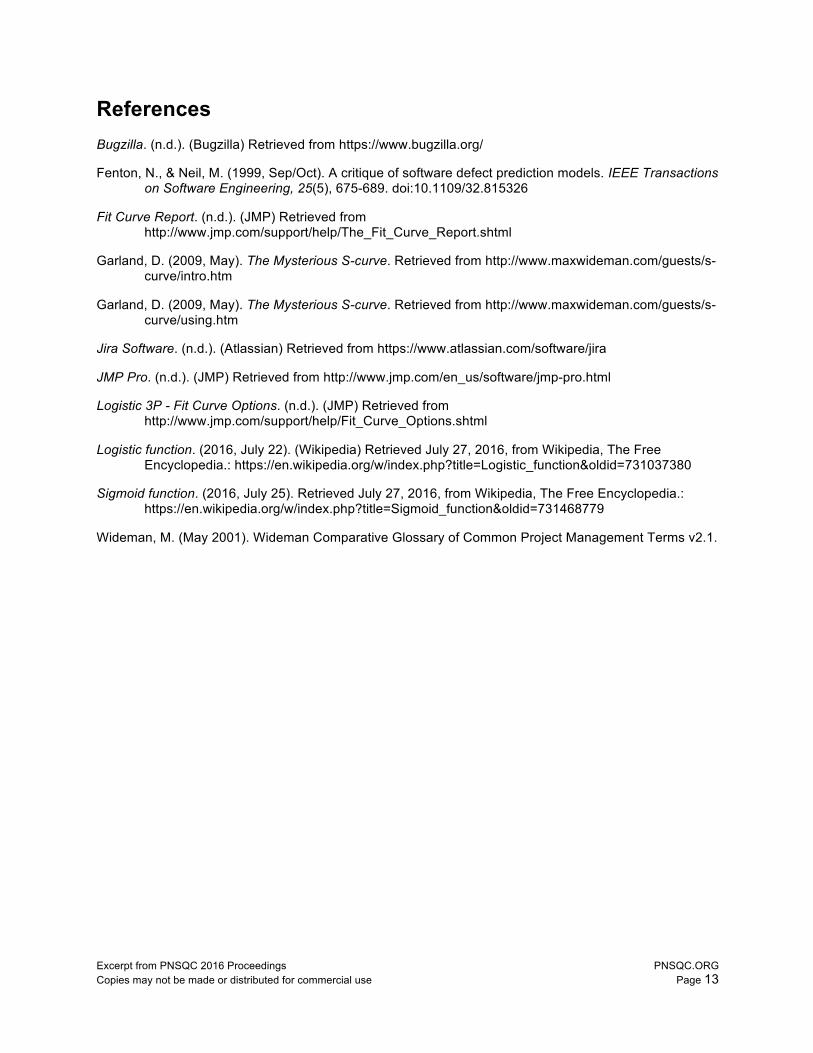
Project Milestones / Parameters Project D with Old PRQ Project D with New PRQ Alpha 12/14/2015 12/14/2015 Beta 2/29/2016 2/29/2016 PRQ 6/13/2016 11/13/2016 Estimated Defect Growth Rate 0.05 0.05 Estimated Inflection Point 130 130 Estimated Asymptote 12282 12282

When we plot the actual trend of the Defects with the milestones, we observe that our PRQ is declared a bit too early. Approximately 55% of the unknown Defects are expected by Beta.


Figure 13: Predicted trend of Project D Vs the Actual Trend

Figure 14: Adjusted PRQ

With the help of this model, we have pushed the PRQ milestone by 5 months and now we account for around 30 – 35 % of the open defects. During this time, we can focus more on the validation such that we further decrease from the 30% mark and come down to 10% open defects. Program Managers can always revisit their assumptions and make necessary changes to the 3 parameters as the project progresses and monitor the S curve trends i.e. actual vs predicted curve.

7 Conclusion Planning a Project schedule and implementing it to the finest is an age old problem faced by Project Management Teams. Our Defect Prediction Model not only eliminates the uncertainty in declaring milestones but also suggests corrective actions during an on-going project. This tool helps the management by predicting the future defects and providing a robust Project schedule. Additionally, we monitor in-process quality of products and take preventive actions on the unforeseen defects/issues/risks. To conclude, we have successfully applied our model to approximately 50 different platforms across different business segments and as a result taken preventive measures in upcoming projects.


References Bugzilla. (n.d.). (Bugzilla) Retrieved from https://www.bugzilla.org/

Fenton, N., & Neil, M. (1999, Sep/Oct). A critique of software defect prediction models. IEEE Transactions on Software Engineering, 25(5), 675-689. doi:10.1109/32.815326

Fit Curve Report. (n.d.). (JMP) Retrieved from http://www.jmp.com/support/help/The_Fit_Curve_Report.shtml

Garland, D. (2009, May). The Mysterious S-curve. Retrieved from http://www.maxwideman.com/guests/s-curve/intro.htm

Garland, D. (2009, May). The Mysterious S-curve. Retrieved from http://www.maxwideman.com/guests/s-curve/using.htm

Jira Software. (n.d.). (Atlassian) Retrieved from https://www.atlassian.com/software/jira

JMP Pro. (n.d.). (JMP) Retrieved from http://www.jmp.com/en_us/software/jmp-pro.html

Logistic 3P - Fit Curve Options. (n.d.). (JMP) Retrieved from http://www.jmp.com/support/help/Fit_Curve_Options.shtml

Logistic function. (2016, July 22). (Wikipedia) Retrieved July 27, 2016, from Wikipedia, The Free Encyclopedia.: https://en.wikipedia.org/w/index.php?title=Logistic_function&oldid=731037380

Sigmoid function. (2016, July 25). Retrieved July 27, 2016, from Wikipedia, The Free Encyclopedia.: https://en.wikipedia.org/w/index.php?title=Sigmoid_function&oldid=731468779

Wideman, M. (May 2001). Wideman Comparative Glossary of Common Project Management Terms v2.1.

Documents

Defect Prediction Model for estimating Project Scheduleuploads.pnsqc.org/2016/papers/45.DefectPrediction... · Defect Prediction Model for estimating Project Schedule Rajesh Yawantikar,