AEDC-TRm 93 m 23

A Critical Evaluation of Methods for Imposing Solid-Wall Boundary Conditions in Inviscid Flow

S. L. Keeling Calspan Corporation/ AEDC Operations

March 1994

Final Report for Period August 1993 - September 1993

Approved for public release; distribution is unlimited.

ARN EN I N PMENT ARNOLD AIR FO TENN

R MATERI M UNITED STATES AIR FORCE

NOTICES

When U. S. Government drawings, specifications, or other data are used for any purpose

oher than a demit re d G r t procurement operation, the Government therebyincurs no responsibility nor any obligation whatsoever, and the fact that the Government

may have formulated, furnished, or in any way supplied the said drawings, specifications,

or other data, is not to be regarded by implication or otherwise, or in any manner licensing

the holder or any other person or corporation, or conveying any rights or permission to

manufacture, use, or sell any patented invention that may in any way be related thereto.

Qualified users may obtain copies of this report from the Defense Technical Informationcenter.I

References to named commercial products in this report are not to be considered in any

sense as an endorsement of the product by the United States Air Force or the Government.

This report has been reviewed by the Office of Public Affairs (PA) and is releasable to

the National Technical Information Service (NTIS). At NTIS, it will be available to the

general public, including foreign nations.

APPROVAL STATEMENT

This report has been reviewed and approved.

MURRAY 0. KINGAeronautical Systems DivisionDirectorate of Aerospace Flight Dynamics Test

Deputy for Operations

Approved for publication:

FOR THE COMMANDER

EUGENE J. SANDERSChief, Aeronautical System FlightDirectorate of Aerospace Flight Dynamics Test

Test Operations Directorate

REPORT DOCUMENTATION PAGE Form Approved

OMB No. 0704-0188

Public reporting burden for this collection of information is estimated to average 1 hour per response, including the time for reviewing instructions, searching existing data sources, gathering and maintaining the data needed, and completing and reviewing the collection of information. Send comments regarding this burden estimate or any other aspect of this collection of information, including suggestions for reducing this burden, to Washington Headquarters Services. Directorate for Information Operations and Reports, 1215 Jefferson Davis Hiohwav. Suite 1204. Arlinoton. VA 22202·4302. and to the Office of Manaoement and Budoet. Paperwork Reduction PrO'ect (Q704-0166i. Washinoton. DC 20503.

1. AGENCY USE ONLY (Leave blank) 12. REPORT DATE March 1994

13. REPORT TYPE AND DATES COVERED Final- August 1993 - September 1993

4. TITLE AND SUBTITLE 5. FUNDING NUMBERS

A Critical Evaluation of Methods for Imposing Solid-Wall 27590F Boundary Conditions in Inviscid Flow 9A22

6. AUTHOR(S) S. L. Keeling Calspan Corporation/AEDC Operations

7. PERFORMING ORGANIZATION NAME(S) AND ADDRESS(ES) 8. PERFORMING ORGANIZATION REPORT NUMBER

Arnold Engineering Development Center/DOFA Air Force Materiel Command AEDC-TR-93-23 Arnold Air Force Base, TN 37389-6000

9. SPONSORING/MONITORING AGENCY NAMES(S) AND ADDRESS(ES) 10. SPONSORING/MONITORING AGENCY REPORT NUMBER

Air Force SEEK EAGLE Office/SK Eglin Air Force Base, FL 32542-6865

11. SUPPLEMENTARY NOTES

Available in Defense Technical Information Center (DTIC).

12a. DISTRIBUTION/AVAILABILITY STATEMENT 12b. DISTRIBUTION CODE

Approved for public release; distribution is unlimited.

13. ABSTRACT (Maximum 200 words)

This report presents a criticai evaluation of wideiy used methods for imposing discrete solid-wall boundary conditions for the numerical computation of inviscid flows. Specifically, it shows that some of these methods are only provisionally correct. Also, an explanation is given for the success of others. In particular, the report shows that a method involving contravariant velocity components can lenerate distortions in computed flows. Because complex CFD calculations can be dif icult to interpret, the claims made here are demonstrated with explicit solutions to simple model problems_ This work emphasizes that subtle and erroneous effects can result from the use of apparently natural numerical methods. It also emphasizes the importance of developing simple tests for these computational methods to elucidate the possible consequences of their use.

14. SUBJECT TERMS

solid-wall boundary inviscid flows

117. SECURITY CLASSIFICATION OF REPORT UNCLASSIFIED

COMPUTER GENERATED

velocity computational methods

18. SECURITY CLASSIFICATION 19. SECURITY CLASSIFICATION OFTHIS PAGE OF ABSTRACT UNCLASSIFIED UNCLASSIFIED

15. NUMBER OF PAGES 40

16. PRICE CODE

120. LIMITATION OF ABSTRACT

SAME AS REPORT Standard Form 298 (Rev, 2-89) Prescribed by ANSI Std. Z39·18 296-102

AEDC-TR-93-23

PREFACE

The work reported herein was conducted at the Arnold Engineering Development Center (AEDC), Air Force Materiel Command (AFMC), under Program Element 27590F, Control Number 9A22, at the request of the Air Force SEEK EAGLE Office (AFSEO/SKM), Eglin Air Force Base, FL. The AFSEO Project Manager was Maj. Larry D. Williams, and the AEDC/DOF A Project Manager was Murray King. David Carlson was the Calspan Project Manager. The work was performed by Calspan Corporationl AEDC Operations, support contractor for aerodynamic testing at AEDC, AFMC, Arnold Air Force Base, TN. The work was performed between August 1993 and September 1993, under AEDC Job Number 0724. The manuscript was submitted for publication on February 8, 1994.

1

AEDC-TR-93-23

CONTENTS

1.0 INTRODUCTION ...................................................... 5 2.0 NOTATIONS AND ASSUMPTIONS ..................................... 6 3.0 DEFINITION OF METHODS ........................................... 9

3.1 Method 1 ......................................................... 9 3.2 Method 2 ......................................................... 14 3.3 Method 3 ......................................................... 14

4.0 ANALYSIS OF METHODS ............................................. 15 4.1 Problem 1 ......................................................... 15 4.2 Problem 2 ......................................................... 16 4.3 Analysis of Method 1 ............................................... 19 4.4 Analysis of Method 2 ............................................... 20 4.5 Analysis of Method 3 ............................................... 20

5.0 OTHER SOLID-WALL CONDITIONS ................................... 21 6.0 CONCLUDING REMARKS ............................................. 22

REFERENCES ......................................................... 23

ILLUSTRATIONS

1. Principal Basis Vectors for Problem 1 ..................................... 16 2. Reciprocal Basis Vectors for Problem 1 ................................... 16 3. Principal Basis Vectors for Problem 2 (z and ~

Coordinates Suppressed) ... ,., ........................................... 18 4. Reciprocal Basis Vectors for Problem 2 (z and ~

Coordinates Suppressed) ................................................. 18

APPENDICES

A. Derivation of Orthogonal Transformation ................................. 25 B. Derivation of Continuum Condition ...................................... 28 C. Detailed Calculations for Analysis of Method 2 ............................ 32

NOMENCLATURE .................................................... 35

3

AEDC-TR-93-23

1.0 INTRODUCTION

In this report, three widely used methods for imposing discrete solid-wall boundary conditions for the numerical computation of inviscid flows are presented, and two of these

methods are shown to offer only provisionally correct results. Specifically, it is shown that

a method involving contravariant velocity components can generate distortions in computed

flows. This method has been used for years in the AIR3D code (Ref. 1) and its derivatives

to compute steady-state flows in stationary grid systems. Also, with the inclusion of time

metrics, this method has been used to compute flows in moving grid systems (Ref. 2).

Steady-state computations performed with these codes have shown that distortions can

be generated in computed flows when grid lines emanating from a solid boundary are not

orthogonal to the wall. The consequences of grid skewness are discussed in Ref. 3. In addition,

it is shown here that the method of contravariant velocity components is correct only if grid lines emanating from solid walls are normally oriented. Because complex CFD calculations

can be difficult to interpret, the claims made here are demonstrated with explicit solutions to simple model problems.

Instead of the above procedure for determining velocity at solid boundaries, there is a more direct approach of simply extrapolating velocity to the wall and subtracting the normal

component. Such a method gives correct results on a stationary grid without conditions on

the grid, such as the orthogonality constraint mentioned above. While this more direct

approach has an unambiguous implementation for stationary grid systems, there are various ways to employ the idea for moving grid systems. Furthermore, some of these implementations

for dynamic grid systems can cause spurious features in computed flows. A correct implementation is proposed and compared with another apparently natural one. Again, since

complex CFD calculations can be difficult to interpret, comparisons are made on the basis

of explicit solutions to simple model problems. Finally, the correct method is shown to be

consistent with solid-wall boundary conditions imposed in Ref. 4. Also, an explanation is given for the use in Ref. 5 of a solid-wall boundary condition for pressure in moving grid systems.

The contents of the report can he summarized as follows. In Section 2.0, the necessary notations and assumptions are presented. In Section 3.0, definitions are given for three methods of imposing discrete solid-wall boundary conditions in moving grid systems for the numerical

computation of inviscid flows. As appropriate, the boundary conditions given are simplified for the treatment of stationary grid systems. Then in Section 4.0, simple examples are presented

to demonstrate which boundary conditions from Section 3.0 give correct numerical results.

In Section 5.0, the numerical boundary conditions used in Refs. 4 and 5 are discussed. Finally, in Section 6.0, the conclusions of this study are summarized.

5

AEDC-TR-93-23

2.0 NOTATIONS AND ASSUMPTIONS

Before any discussion of discrete boundary conditions can begin, the continuum boundary condition must be given together with a description of the kind of applications for which it is intended. Also, since CFD codes do not all operate in the same way, the present numerical orientation must be explained and certain notations must be developed.

Assume that a solid body is in rigid motion with respect to what will be called a stationary frame. Let stationary frame Cartesian coordinates be given by

% = [x,y,z]T = [Xb X2,X3f.

Also, let curvilinear coordinates

be established around the moving body for the purpose of defining a computational grid. Specifically, at every time level, tn, grid points (%')./' ~) satisfy

(1)

That is, the curvilinear coordinates assume integer values at grid points. Also, it is assumed that for every fixed time, t, the transformation from % to ~ is well-behaved in the sense that

(2)

satisfies

o < /1 ::; det {J} ::; /2 < 00 (3)

for constants 1'1 and 1'2' Therefore, the inverse transformation from ~ to % is well-behaved. Also, it follows from the chain rule expressions,

(4)

6

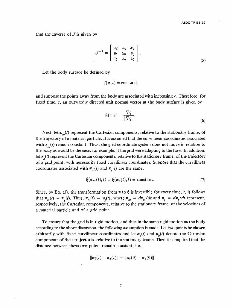
AEDC-TR-93-23

that the inverse of .J is given by

(5)

Let the body surface be defined by

(( x, t) = constant,

and suppose the points away from the body are associated with increasing r. Therefore, for fixed time, t, an outwardly directed unit normal vector at the body surface is given by

A( ) V( n x,t = IIV(II'

(6)

Next, let zm(t) represent the Cartesian components, relative to the stationary frame, of the trajectory of a material particle, It is assumed that the curvilinear coordinates associated with xm(t) remain constant. Thus, the grid coordinate system does not move in relation to the body as would be the case, for example, if the grid were adapting to the flow. In addition, let x (t) represent the Cartesian components, relative to the stationary frame, of the trajectory g .

of a grid point, with necessarily fixed curvilinear coordinates. Suppose that the curvilinear

coordinates associated with x,it) and zit) are the same,

~(Xm(t), t) = ~(Xg(t), t) = constant. (7)

Since, by Eq. (3), the transformation from = to ~ is invertible for every time, t, it follo\vs

that xm(t) = xit). Thus, 'OnP) = 'Oit), where 'Om = dXm/dt and 'Og = dx/dt represent, respectively, the Cartesian components, relative to the stationary frame, of the velocities of a material particle and of a grid point.

To ensure that the grid is in rigid motion, and thus in the same rigid motion as the body according to the above discussion, the following assumption is made. Let two points be chosen arbitrarily with fixed curvilinear coordinates and let x aCt) and xb(t) denote the Cartesian components of their trajectories relative to the stationary frame. Then it is required that the distance between these two points remain constant, i.e.,

7

AEDC-TR-93-23

As shown in Appendix A, this condition has the important consequence that there is an orthogonal rotation matrix, L(t), i.e.,

(8)

such that

(9)

In particular, let one point correspond to any grid point and let the other correspond to a reference point such as the body's center of gravity. Thus, grid movement can be accomplished knowing only the rotation matrix and the trajectory of a reference point.

The physical condition to be imposed on velocity for a solid-wall boundary condition in inviscid flow is that no fluid pass into the body. Mathematically, this means that the components of fluid velocity relative to the moving frame can have no normal component at the body surface. It is shown in Appendix B that this condition can be stated in the stationary frame as follows,

n . ( 17 - 17m ) = 0 (10)

where 17 = [u, V, W]T represents the Cartesian components of fluid velocity relative to the stationary frame. For a more computationally convenient version of the above equation, the material particle velocity, 17m, can be replaced with the grid velocity, "g' as explained above. Thus, the continuum condition for fluid velocity can be expressed as

n . (17 - 17g ) = O. (11)

Also, "g can be calculated explicitly by differentiating Eq. (7) with respect to t to obtain

Vf.d%g of. = o. dt + at

Recalling that J = Vf., the last equation can be written asJ~ + f.t = 0, or by Eq. (3),

(12)

8

AEDC-TR-93-23

Now, combining Eqs. (6), (12), and (11) gives the condition

or

= o.

Finally, using Eq. (4), the continuum condition can be written as

(13)

3.0 DEFINITION OF METHODS

Equation (11) above shows that, for a grid point on the body surface, the normal component of fluid velocity must be set equal to that of grid velocity. However, this condition gives no indication of how the tangential components should be calculated. This is the crucial point; after all, there are many ways to satisfy Eq. (11), including setting 11 = 11 g' To guarantee continuity of the tangential component at the wall, some form of extrapolation from the field must be used. First, a method involving contravariant velocity components is described. Then, two other more direct methods are defined.

3.1 METHOD 1

For a description of Method 1, a careful definition is given first for the contravariant components of vectors in four-dimensional space-time. Let "it) = [xit) , yit) , zit)]T represent the Cartesian components, relative to the stationary frame, of the trajectory of a fluid particle, so that its world line is represented by [xit), yit), zit), tf. In other words, with {ex' cy ' ez, ell} denoting a Cartesian basis for space-time, the world line is given by

Its temporal derivative is given by

9

AEDC-TR-93-23

where again 11 = [U, V, w]T represents the Cartesian components of fluid velocity relative to

the stationary frame. Now suppose curvilinear coordinates (~,..",t,r) = (~1'~2'~3'~4) are established for space-time. Also, suppose that X(~,'l7,t,r) is defined so that curvilinear coordinate curves are obtained by fixing three of the arguments in X while varying the fourth. Thus, a principal basis for space-time is given by {Xf X'I/' X I' X

r}, and the corresponding

reciprocal basis is given by {V~, V..", Vt, Vr} where, for example, V~ is defined by

(14)

These bases have the property that X~i • V~j = oij' Also, X~i is tangent to the ~i coordinate line with constant ~Ni' while V~j is ortho~onal to the hypersurface of constant ~j' For a 4-vector, say U, the covariant components, (Ul'U2,U3,U4), are defined by

4 4

U = ~UjVej, where U . X~i = 'LUj6ij = Ui. j=l j=l

Also, the contravariant components, (U1 ,U2, U3, U4), are defined by"

4

U = Lujx~j' j=l

where 4

U· Vei = L Uj6ij = Ui.

j=l

Therefore, the contravariant components, {a, v, W,S}, of V satisfy

where

u V·V~

v V·VrJ UrJx + vrJy + WrJz + rJt

W V·V(

S V·VT UTx + VTy + WTz + Tt. (15)

* This terminology originates from the fact that if the coordinate system were changed, the transformation from the old to the new covariant components has the same form as the transformation from the old to the new principal basis vectors. On the other hand, the transformation of the contravariant components is different from that of the principal basis vectors, but has the same form as that for reciprocal basis vectors.

10

AEDC-TR-93-23

Finally, in view of Eq. (13), the continuum boundary condition can be expressed as

w=o (16)

where W is the contravariant component of the space-time vector V given above.

It has become customary to refer to V, V, and W as the contravariant components of velocity even when~, YJ, and t are time-varying. However, this use of terminology from tensor analysis is not strictly correct. In fact, by Eq. (3), {zp ZII' z!V and {V~,VYJ,Vn form principal and reciprocal bases for three-dimensional space at any given time t. Calculations similar to those prior to Eq. (15) show that the contravariant components of velocity are 11 • V~,

11 • VYJ, and 11 • Vt, i.e.,

Of course, these components coincide with V, V; and W when ~, YJ, and t are time-independent.

The solid-wall boundary condition as shown in Eq. (16) has been implemented numerically according to a procedure that is distilled below to a single equation, Eq. (21). This equation is not used widely, but it is important for comparison with other methods. Also, it provides a means for representing the present method in compact form. There are many variants of this method, but the condition derived serves as a representative of procedures involving contravariant components.

The numerical implementation of Eq. (16) proceeds as follows. First, the Cartesian components of fluid velocity are extrapolated to the solid surface, where t = 1= 1, from the first point off the wall, where S = 1= 2. Then the components, U, V, and Ware determined. By Eqs. (15) and (2) this process can be written as

[V 1 n [ ~t 1 n [ U 1 n V TJt + :T]kl V

W jkl (t jkl W jk2 (18)

t If ris independent of x, y, and z, then the vector sets, {Sf slI,sr} and {X~,X1j,Xr}, are identical.

11

AEDC-TR-93-23

Following Eq. (16), the next step is to set W to zero by multiplying the last equation by

[I - M], where

(19)

Next, the result of this multiplication is translated to Cartesian components. Again, using

Eqs. (15) and (2), this process can be written as,

[ u 1 n -1 [ et 1 n -1 [ U 1 n v = - (J"]11) TIt + (J"Ik1) [I - M] V W jk1 (t jk1 W jk1 (20)

Now, fJ.1/ki 1 is explicitly equated with fJ'fr1 and Eq. (18) is substituted into Eq. (20) to obtain,

[ ~ 1 n+1 = - (.1;11 r1 [ ~: 1 n + (J"}kl) -1 [I - M] { [ ~: 1 n + J"Ikl [ ~ 1 n }.

W jkl (t jkl (t jkl W jk2

As seen below, the expression in braces can be expressed in terms of fluid velocity and grid

velocity by factoring out J")k1' For this, the product, J"lkl (.J lk1 ) -1 is inserted after [1 - M.1. After some algebra, the following is obtained,

The bracketed expression can be simplified with the following explicit calculation,

[

. . x( 1 n [0 0 1- . . y( 0 0

. . z( jkl 0 0

12

AEDC-TR-93-23

Combining the last two equations and Eq. (12) gives

or

(21)

This will be referred to as Method 1 for setting inviscid flow velocity at a solid-wall boundary. The crucial element on which to focus is the presence of the term, %\' This vector is tangent to the coordinate line emanating from the the body surface, and it is not normally oriented unless % \ and V'r are parallel. In Subsection 4.3, it is shown that this aspect of Method 1 causes spurious disturbances to be generated in computed flows.

Finally, to complete the definition of Method 1, the grid velocity is specified with a discrete formula instead of Eq. (12). Since flg=dz/dt, the local grid velocity at time level, tn, can be approximated using grid point coordinates at time levels, ~ and tn - 1,

(22)

Now, instead of storing the old grid, zfl<ll can be computed from zftcl as suggested following Eq. (9). Specifically, suppose the grid movement is characterized by the trajectory of a reference point zo(t) and a rotation matrix, L(t). Then by Eq. (9),

[ ~n _ (tn \] _ T (-In) [_0 (-10\] "'-jkl - "'-0 ) -.LJ. ""jkl - :1:0 • )

and

Using Eq. (8) to eliminate [zJkl - %o(to)] between these equations gives

(23)

13

AEDC-TR-93-23

Thus, by combining Eqs. (22) and (23), the grid velocity is computed equivalently according to Eq. (22) or

(24)

3.2 METHOD 2

Method 2 for setting the inviscid flow velocity is a more direct numerical formulation ofEq. (11), which has also been used in AIR3D. The basis of the method is as follows. Working in the moving frame, the velocity at time level, tn, is extrapolated to the solid surface from the first point off the wall. Then the normal component is subtracted, and the result is expressed in the stationary frame. Finally, the velocity obtained is used at the wall for time level, tn + 1 •

Using the techniques of Appendix B, and Eqs. (B-6) and (B-7) in particular, this procedure can be expressed purely in the stationary frame as

n+l _ ( )n + [I A AT] n ( )n fljkl - 'fig jkl - nn jkl 'fI - 'fig jk2'

Using Eq. (6), Method 2 can be written as

'\7 (n n+l ()n ( )n jkl [v(n • ('fI _ 'fI)n ]

fljkl = fig jkl + 'fI - 'fig jk2 - IIV' (jk111 2 jkl g jk2 . (25)

with the grid velocity computed according to Eq. (24).

Method 2 appears natural because it is consistent with a standard condition posed in the moving frame with respect to which the grid velocity is zero. However, as shown in Subsection 4.4, Method 2 causes spurious disturbances to emerge in computed flows because 'fig is evaluated at more than one point in the above equation. Specifically, this creates a problem in cases where the moving frame is noninertial and the grid velocity varies throughout the grid.

3.3 METHOD 3

Finally, Method 3 for setting the inviscid flow velocity is derived from Method 2 by making modifications to avoid the spurious effects shown in Subsection 4.4 in connection with Method 2. Specifically, the present method is posed so that the grid velocity is always evaluated at a single point. Method 3 can be written compactly as

n+l_()n [I AAT]n In. ()n] I1jkl - 'fig jkl + - nn jkl I1jk2 - fig jkl .

14

AEDC-TR-93-23

Using Eq. (6), this can be written as

(26)

with the grid velocity computed according to Eq. (24). It is shown in Subsection 4.5 that Method 3 passes the tests developed in the next section.

4.0 ANALYSIS OF METHODS

Methods 1, 2, and 3 are analyzed in terms of their performance for two simple model problems. In the first model problem, the inviscid flow is over a flat plate. Also, the grid is stationary and grid lines emanating from the plate have a nonnormal orientation. In the second example, the inviscid fluid is at rest around a rotating cylinder. Here the grid is in rigid motion with the solid body.

4.1 PROBLEM 1

For model Problem 1, let a flat plate be located at z = 0 and the field at z > O. Also, assume that the fluid velocity distribution, '11 = [u, v, wf, is two-dimensional with v = O. The components, u and w, can be chosen arbitrarily to satisfy the Euler equations, provided w = 0 only at z = O. Thus, a proper boundary condition will not introduce a nonzero v component to the velocity.

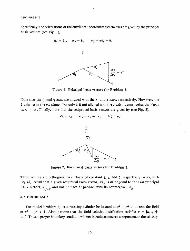
The curvilinear coordinate system for Problem 1 is time-independent and is defined as follows,

~ = x, TJ = Y -,z, ( = z. (27)

To show the skewness of this coordinate system, the orientation of the coordinate axes is now computed. For example, the ~-axis is defined as the line along which 1] and t are constant. So, the position vector, % = [X,y,Z]T, is a function only of ~ along this line. Therefore, %~ is tangent to the ~-axis. Similarly, %." and %1 give the orientations of the 1]- and t-axes, respectively. These can be calculated from

15

AEDC-TR-93-23

Specifically, the orientations of the curvilinear coordinate system axes are given by the principal basis vectors (see Fig. 1),

x

Figure 1. Principal basis vectors for Problem 1.

Note that the ~- and 'l1-axes are aligned with the x- and y-axes, respectively. However, the r-axis lies in the y,z plane. Not only is it not aligned with the z-axis, it approaches the y~axis

as 'Y -- 00, Finally, note that the reciprocal basis vectors are given by (see Fig. 2),

V'~ = ex, V''f} = ey -,ez , V'( = ez •

/'e x/

Figure 2. Reciprocal basis vectors for Problem 1.

These vectors are orthogonal to surfaces of constant ~, ,/}, and r, respectively. Also, with Eq. (4), recall that a given reciprocal basis vector, V'~i' is orthogonal to the two principal

basis vectors, z~Ni' and has unit scalar product with its counterpart, z~;'

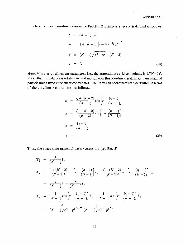
4.2 PROBLEM 2

For model Problem 2, let a rotating cylinder be located at x2 + y2 = 1, and the field at x2 + y2 > 1. Also, assume that the fluid velocity distribution satisfies v = [u, v, w] T

= O. Thus, a proper boundary condition will not introduce nonzero components to the velocity.

16

AEDC·TR·93·23

The curvilinear coordinate system for Problem 2 is time-varying and is defined as follows,

e (N - 1)z + 1

ry = 1 + (N - 1) [t - tan-1 (y/x)]

( = (N - 1 hi x2 + y2 - (N - 2)

T = t. (28)

Here, Nis a grid refinement parameter, i.e., the approximate grid cell volume is 1/(N-l)3.

Recall that the cylinder is rotating in rigid motion with this coordinate system, i.e., any material particle holds fixed curvilinear coordinates. The Cartesian coordinates can be written in terms of the curvilinear coordinates as follows,

x = (+(N-2) [ (ry-1)] (N - 1) cos T - (N - 1)

y = (+(N-2) . [ (ry-1)] (N - 1) SIll T - (N - 1)

z = (e - 1) (N -1)

t = T. (29)

Thus, the space-time principal basis vectors are (see Fig. 3)

~ 1 A

~e = (N_1)eZ

(+(N-2). [ (ry-1)] A (+(N-2) [ (ry-1)]A Xry = (N _ 1)2 SIll T - (N _ 1) ex - (N _ 1)2 cos T - (N _ 1) ey

Y A X A

(N - 1) ex - (N _ 1) ey

'V 1 [(ry-1)]A 1. [ (ry-1)]A A, (N _ 1) cos r - (N _ 1) ex + (N _ 1) SIll T - (N _ 1) ey

X A Y A = e + e (N - 1)Jx2 + y2 x (N - 1)Jx2 + y2 y

17

AEDC-TR-93-23

(+(N-2) . [ (17-1)], (+(N-2) [ (17- 1)], , - (N - 1) sm 7 - (N _ 1) ex + (N _ 1) cos 7 - (N _ 1) ey + et

..

x y X,

Figure 3. Principal basis vectors for Problem 2 (z and ~ coordinates suppressed).

and the reciprocal basis vectors are (see Fig. 4)

(N - 1)ez

(N - 1)y, (N - 1)x , 1 '

2 + 2 ex - 2 + 2 ey + (N - ~ )et x y x y

1)(

1)7

1)7

x

1)(

Figure 4. Reciprocal basis vectors for Problem 2 (z and ~ coordinates suppressed).

18

AEDC-TR-93-23

4.3 ANALYSIS OF METHOD 1

Now, consider the application of Method 1 in Eq. (21) to Problem 1. Since the curvilinear coordinate system is time-independent, the grid velocity is zero. Also, since Zs- = 'Ye

y + e

z and Vr = ez' Eq. (21) becomes

[:L [:L-[I] [0 0 1] [ ]0 [ ]0 [ ]0 u u u

v v - 'Yw -,w

W jk2 0 jk2 0 jk2

for the first time step. Note that the last equality follows since it is assumed that the flow is two-dimensional with the v component zero. However, this method creates a v component, v)kl = - 'YwJk2' at the wall which is propagated into the field. In fact, the problem is made worse with more skewness in the grid, i.e., as'Y - 00. Since Method 1 generates this disturbance in the flow, it is judged to be unacceptable.

On the other hand, if the nontangential grid lines are orthogonal to the body surface, Method 1 produces correct boundary values. This can be seen by setting 'Y = 0 in Problem 1 so that Zs- = ez and v)kl = O. In general, under the condition that nontangential grid lines are orthogonal to the body surface, Method 1 can be rewritten as follows. Equation (21) must be modified to reflect the constraint that z s- must be orthogonal to the wall. Since V r is always orthogonal to the wall, it must be that Zs- = cVr for some scalar c. On the other hand, since z s- and V r are principal and reciprocal basis vectors, respectively, from Eq. (4)

it follows that Zs- • V r = 1. Therefore,

Under the new constraint, Method 1 takes the form,

'\7(n n+l n jkl {'\7(n [n ()n] } 'Djkl = l1jk2 - 11'\7(jklIl2 jkl' l1jk2 - l1g jkl

with 11 g computed according to Eq. (24). In other words, under the orthogonality condition, Eqs. (21) and (26) are identical.

The flaw in Method 1 can be understood most easily as follows. For simplicity, assume that the grid system is time-invariant. Then the fluid velocity can be written as shown in Eq. (17),

19

AEDC-TR-93-23

Consider this in relation to Fig. 1. Since %~ and %11 always lie in the tangent plane of the body surface; setting '0 • V r = W = 0 does indeed make '0 purely tangential. However, with skewness in the grid, :1:\ has a tangential part. Thus, setting W = 0 modifies the tangential part of '0.

4.4 ANALYSIS OF METHOD 2

Now consider the application of Method 2 in Eq. (25) to Problem 2. Since the fluid velocity is assumed to be zero everywhere initially, the method becomes

(30)

for the first time step. By the steps shown in Appendix C, the following is obtained,

_ (N + 1) 1 - cos(~t) [ X~kl 1 (N - 1) ~t Yjk1'

o

The first term on the right side of this equation is a consequence of the difference, ('0 g)Jkl

- ('Og)Jk2' appearing in Eq. (30). Note that even in the limit as fl.! -- 0, this term does not vanish, and the boundary velocity is given by

Thus, this method creates nonzero velocity components at the wall which are propagated into the field. Based on the correspondence between terms in the equations above, the disturbance is related directly to the fact that the grid velocity is evaluated at more than one point in Eq. (25). On the other hand, the magnitude of the initial disturbance is diminished with grid refinement, i.e., as N -> 00. Nevertheless, since Method 2 generates this disturbance in the quiescent flow, it is judged to be unacceptable.

4.5 ANALYSIS OF METHOD 3

Now consider the application of Method 3 to Problem 1 and then Problem 2. For Problem 1, the curvilinear coordinate system is time-independent, so the grid velocity is zero. Also, since Vr = cz' Eq. (26) becomes

20

AEDC-TR-93-23

[0 0 1]

for the first time step. Note that the last equality follows since it is assumed that the flow is two-dimensional with the v component zero. Since Method 3 does not spuriously generate a v component in the field, it is judged acceptable in terms of Problem 1.

Now consider the application of Method 3 to Problem 2. Since the fluid velocity is assumed to be zero everywhere initially, the method becomes

(31)

for the first time step. By the same steps as shown for Method 2, the following is obtained,

1 1 - cos(~t) [ X~kl 1 'Djkl = f:1t Yjkl'

o

As t:..t -- 0, the velocity introduced at the wall vanishes. In fact, in the limit, the grid velocity is computed exactly and vJkl = O. On the basis of these examples, Method 3 is judged superior to Methods 1 and 2.

5.0 OTHER SOLID-WALL CONDITIONS

After Method 3 was derived, it was later found to be consistent with a scheme used in Ref. 4. A node-centered version of the method for setting the boundary velocity is given by,

(32)

That the condition on velocity is equivalent to that shown in Eq. (26) for Method 3 can be seen as follows. By Eqs. (12), (2), and (5),

[

~x - \1(- Vg = \1(T [J-l~t] = [0 0 1] Tlx

(x

21

AEDC-TR-93-23

Thus, the right side of Eq. (26) is

V (n n jkl {V(n n v(n ( )n }

"jk2 - IIV(jklIl2 jkl . "jk2 - jkl' "g jkl

v(n n jkl {V(n n (()n} = "jk2 - IIV(jhIl2 jkl • "jk2 + t jkl

which is on the right side of Eq. (32).

Next, the following solid-wall boundary condition for pressure is imposed in Ref. 5,

ap , an = -pa.g • n. (33)

Here, n is an outwardly directed unit normal vector at the body surface, and alan denotes a directional derivative in the direction of n. Also, lig represents the grid acceleration. The basis of this boundary condition can be understood as follows. First, the conservation of momentum can be written as

d" pa. = p dt = - V p.

Here, dvl dt denotes the total derivative of fluid velocity which is, of course, equal to the fluid acceleration, Ii. Now, in addition to imposing Eq. (11) so that the normal component of fluid velocity and grid velocity are identical, one may naturally require the same condition for the fluid and grid accelerations,

Finally, when this equation is combined with the normal component of the preceding one, the condition in Eq. (33) is obtained.

6.0 CONCLUDING REMARKS

This work emphasizes that subtle and erroneous effects can result from the use of apparently natural numerical methods. It also underscores the importance of developing simple tests for these computational methods to elucidate the possible consequences of their use. In this report, simple model problems were used to test three methods for imposing discrete solid-wall boundary conditions for the numerical computation of inviscid flows. The methods considered were applied in stationary and moving grid systems. It was shown that two of these methods are only provisionally correct. In particular, a well-known method involving

22

AEDC-TR-93-23

contravariant velocity components was shown to provide correct solid-wall boundary values only if grid lines emanating from the solid boundary are normally oriented at the wall. Specifically, this report shows that without the orthogonality constraint, the method corrupts the tangential component of the velocity extrapolated from the field. Also, another more direct method was shown to provide correct solid-wall boundary values only if the grid velocity is uniform, as is the case when the frame of the moving body is inertial. Otherwise, the differences between grid velocities, evaluated at different points for the method, disturb the boundary values. Finally, a correct procedure was posed to avoid the problems of the other two methods, and this procedure was shown to pass tests developed herein.

REFERENCES

1. Pulliam, T. H. and Steger, J. L. "On Implicit Finite Differences of Three-Dimensional Flows." AIAA 78-10, January 1978.

2. Dougherty, F. C., Benek, J. A. and Steger, J. L. "On Applications of Chimera Grid Schemes to Store Separation." NASA-TM-99193, October 1985.

3. Thompson, J. F., Warsi, Z. U. A., and Mastin, C. W. Numerical Grid Generation: Foundations and Applications, North Holland, New York, Amsterdam, Oxford, 1985.

4. Belk, D. M., Janus, J. M., and Whitfield, D. L. "Three-Dimensional Unsteady Euler Equations Solutions on Dynamic Grids." AFATL-TR-86-21, April 1986.

5. Stanek, M. J. and Visbal, M. R. "Investigation of Vortex Development on a Pitching Slender Body of Revolution." AIAA-91-3272-CP.

23

AEDC-TR-93-23

APPENDIX A DERIVATION OF ORTHOGONAL TRANSFORMATION

In this appendix it is shown that if a system is in rigid motion, i.e.,

(A-I)

where ~a(t) and %b(t) represent Cartesian components, relative to the stationary frame, of any two points that are fixed in the moving frame, then there is an orthogonal matrix, L(t), i.e.,

(A-2)

such that

(A-3)

For this, define a vector-value function, t, by

l(z(O) - %0(0), t) = ~(t) - ~o(t). (A-4)

where ~(t) and %o(t) represent Cartesian components, relative to the stationary frame, of two points that are fixed in the moving frame. In other words, l performs a rigid motion on the vector, %(0) -%0(0), and produces ~(t) - zo(t) after time t. To achieve the result of Eq. (A-3), twill be shown to be linear in its first argument and representable in terms of an orthogonal matrix.

First, it is shown that l preserves scalar products, i.e., for any vectors, z and fI,

l(z, t) .t(fI, t) = z . fl. (A-5)

For this, %(t) and y(t) represent points fixed in the moving frame such that

~(O) - ~0(0) = z and y(O) - zo(O) = fl. (A-6)

Then, using the identity

25

AEDC-TR-93-23

and the definition of I gives

l(z(O) - zo(O), t) ·1(y(O) - zo(O), t) = [z(t) - zo(t)] . [y(t) - zo(t)]

By Eq. (A-I),

1 1 l(z(O) - zo(O), t) ·1(y(O) - zo(O), t) = -llz(O) - zo(0)112 + -11;,(0) - zo(0)112

2 . 2

Equation (A-5) now follows from the above equations.

This fact is now used to show that

Ill(ax + f3j,t) - al(x,t) - f31(j,t)1I 2 = 0

and hence that I is linear in its first argument. Using Eq. (A-5) ,

III (ax + f3j, t) - al(x,t) - f31 (j,t)1I 2

= l(ax + (Jj,t) ·l(ax + (Jj,t) + a2l(x,t) ·l(x,t) + (J2l(j,t) .l(j,t)

-2al(ax + f3j, t) .l(x,t) - 2f31(ax + f3j, t) ·l(j,t) - 2af3l(x,t) ·l(j, t)

-2a (ax + f3j). x - 2f3 (ax + f3j). fJ - 2af3x . fJ

= III ax + f3fJ) - ax - f3j1l2 = O.

Thus, I is linear in its first argument and can be written in terms of a matrix, L(t), as

l(x,t) = L(t)z. (A-7)

26

AEDC-TR-93-23

To see that L(t) must be orthogonal, note that by Eqs. (A-5) and (A-7)

Since z and fI are arbitrary, they can be chosen as x = ei and j = ej to obtain

e[ LT(t)L(t)e[ = bij.

In other words, Eq. (A-2) holds. Finally,

L(t) [Zb(O) - za(O)] = L(t) {[Zb(O) - zo(O)] - [za(O) - zo(O)]}

= 1 (Zb(O) - zo(O), t) -l (za(O) - zo(O), t)

= [Zb(t) - zo(t)] - [za(t) - zo(t)]

= [Zb(t) - za(t)].

Thus, Eq. (A-3) is obtained.

27

AEDC-TR-93-23

APPENDIX .B DERIVATION OF CONTINUUM CONDITION

In this appendix, the continuum condition of Eq. (10),

(B-1)

is derived from the more primitive condition,

(B-2)

which applies in the moving frame. Specifically, n represents the Cartesian components, relative to the moving frame, of an outwardly directed unit normal vector at the body surface. Also, v represents the Cartesian components of fluid velocity in the moving frame.

To establish the relationship between the components ofEq. (B-1) in the stationary frame and the components of Eq. (B-2) in the moving frame, the two coordinate systems are related as follows. Specifically, let x and x represent the Cartesian components, relative to the stationary and moving frames, respectively, of any point at time t. Also, suppose zo(t)

represents the Cartesian components, relative to the stationary frame, of a reference point used as the origin in the moving frame. Assume that the two coordinate systems coincide at t = 0 and thus xo(O) = O. Then by Eq. (9), LT(t)~ -xo(t)] represents an initial vector which from time, t = 0, evolves to the vector L(t)LT(t)[x -x'o(t)] = x -xo(t) after time t. Furthermore, the vector remains in rigid motion with respect to the moving frame and hence has unchanging Cartesian components, X, relative to the moving frame. Therefore, since the two coordinate systems coincide initially,

(B-3)

Also, by Eq. (8),

x - xo(t) = L(t)x. (B-4)

Equations (B-3) and (B-4) define the relation between the stationary and moving frame Cartesian systems.

Now, the relation between n of Eq. (6) and n will be determined. For this, let xit)

represent the Cartesian components, relative to the stationary frame, of a point on the

28

AEDC-TR-93-23

boundary. Then define Z b(t) = % a(t) + n(t) to represent a point off the wall at the end of the unit normal vector, n. Since at t = 0, %b(O) -zO<0) = n(O) = n, Eq. (9) gives

n(t) = [Zb(t) - %a(t)] = L(t) [%b(O) - %a(O)] = L(t)n(O) = L(t)n. (B-5)

Also, by Eq. (8),

(B-6)

Next, v will be related to 11 and 11m , Specifically, it will be shown that

(B-7)

For this, let zJt) and zJt) represent the Cartesian components, relative to the stationary and moving frames, respectively, of a fluid particle trajectory. Also, let zm(t) and zm represent the Cartesian components, relative to the stationary and moving frames, respectively, of the trajectory of a material particle at rest in the moving frame. Then define

dZj 11= -,

dt

_ dZj 11=-,

dt

_ dZm 11m = -- = 0,

dt d%o

110 =-. dt

Equation (B-7) will now be established for an arbitrary point in space-time where the fluid particle and material particle traj ectories intersect. Specifically, it is assumed that there is a time, t*, when

Now, by Eq. (B-3),

Differentiating this gives

dLT v(t) = -(t) [% j(t) - zo(t)] + LT(t) [11(t) - 110(t)].

dt

By Eq. (B-4),

Zj(t) - %o(t) = L(t)zj(t).

29

(B-8)

AEDC-TR-93-23

Combining the last two equations gives

(B-9)

To bridge the gap between Eq. (B-9) and Eq. (B-7), the material particle velocity will be expressed in terms of the items appearing on the right side of Eq. (B-9). By Eq. (B-4) ,

By Eq. (B-8),

After differentiation this becomes

MUltiplying this by LT(t) and evaluating the result at t = t* gives

To relate the right side here with the term involving Xj in Eq. (B-9), the following relation is used,

Since L(t) is orthogonal, this follows by differentiating LT(t)L(t) = I. From the last two equations it follows that

(B-IO)

30

AEDC-TR-93-23

Evaluating Eq. (B-9) at t = t* and combining the result with Eq. (B-IO) gives

i(t*) = _LT(t*) [l1m(t*) - vo(t*)] + LT(t*) [v(t*) - vo(t*)]

LT(t*) [v(t*) - vm(t*)].

Since the intersection point of Eq. (B-8) is arbitrary, Eq. (B-7) follows.

Now, combining Eqs. (B-2), (B-6), and (B-7) gives the continuum condition on the fluid velocity expressed in terms of Cartesian components in the stationary frame,

which is the condition of Eq. (B-1).

31

AEDC-TR-93-23

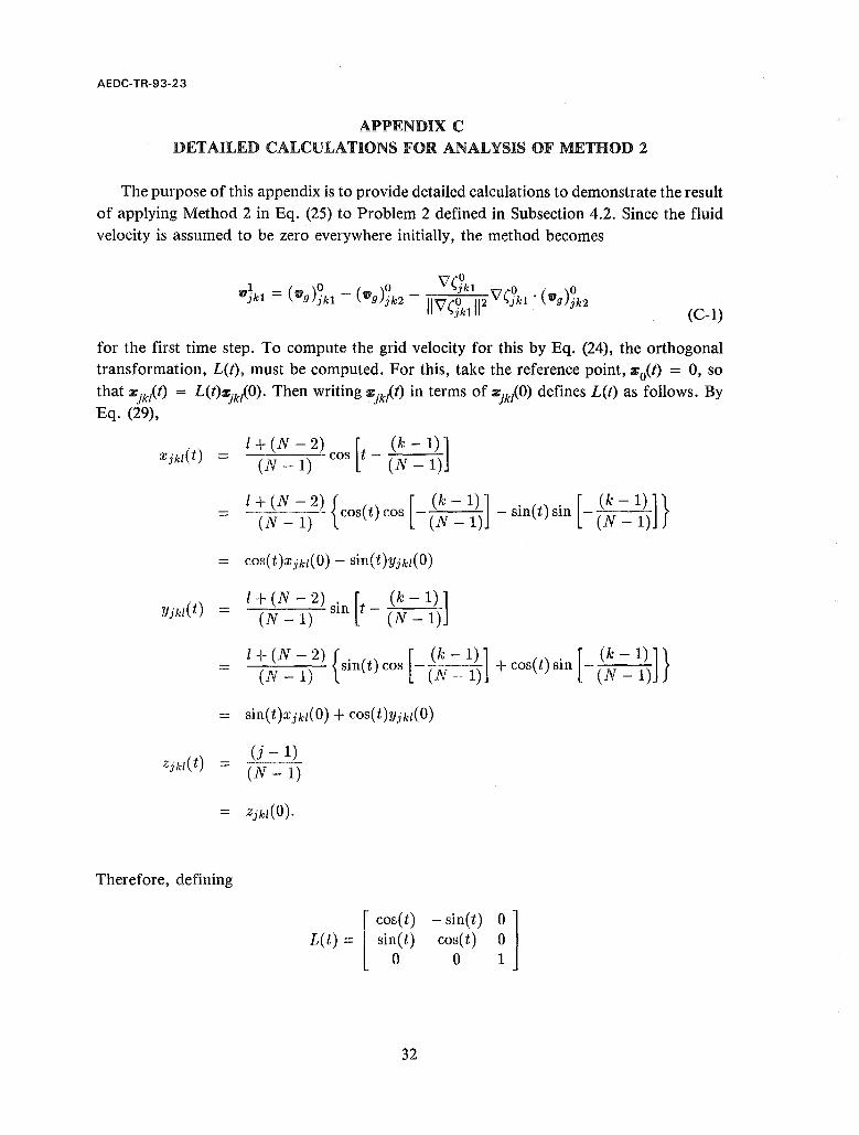
APPENDIX C DETAILED CALCULATIONS FOR ANALYSIS OF METHOD 2

The purpose of this appendix is to provide detailed calculations to demonstrate the result of applying Method 2 in Eq. (25) to Problem 2 defined in Subsection 4.2. Since the fluid velocity is assumed to be zero everywhere initially, the method becomes

VI~ - (VI)O _ (VI )0 \7 (Jkl \7(0 ( )0 Jkl - 9 jkl 9 jk2 - II \7 (Jk111 2 jkl' Vlg jk2

(C-l)

for the first time step. To compute the grid velocity for this by Eq. (24), the orthogonal transformation, L(t), must be computed. For this, take the reference point, %o(t) = 0, so that %jk/(t) = L(t)~k/(O). Then writing %jk/(t) in terms of %jkAO) defines L(t) as follows. By Eq. (29),

1+(N-2) [ (k-l)] Xjkl(t) = (N _ 1) cos t - (N _ 1)

= I ~~~~)2) { cos(t) cos [_ (~ ~ 1{)] _ sin(t) sin [_ (~ ~ 1{)]} = coS(t)Xjkl{O) - sin(t)Yjkl(O)

1+ (N - 2) . [ (k - 1)] Yjkl(t) = (N _ 1) sm t - (N _ 1)

= I ~ ~ ~)2) {sin( t) cos [_ (~l ~ 1{)] + cos( t) sin [_ (~ ~ 1{)] }

= sin(t)Xjkl(O) + coS(t)Yjkl(O)

(j - 1) = (N - 1)

= Zjkl(O).

Therefore, defining

[

cos(t) L(t) = Si~(t)

32

- sin(t) O~ 1 cos(t)

o

AEDC-TR-93-23

satisfies the equation, %jkl(f) = L(f)':I!jkl(O). Thus, by Eq. (24) the grid velocity is given by

which simplifies to

(C-2)

Now, since

0 Xjkl = [ (k-1)]

cos - (N _ 1) 0

Xjk2 = N [(k - 1)] (N - 1) cos - (N - 1) = N 0

(N - 1) Xjkl

0 . [ (k - 1)] 0 N . [ (k - 1) 1 N 0 Yjkl = sm - ( ) Yjk2 = (N - 1) sm - (N - 1L = (N - 1)Yjkl N -1

0 (j - 1) 0 (j - 1) Zjkl = Zjk2 = (N -1) (N - 1) (C-3)

the first two terms in Eq. (C-l) are given by

(C-4)

Next, by Eq. (28), vrJkl in Eq. (C-l) is given by

33

AEDC-TR-93-23

(C-5)

since (ijkl)2 + (yJkl = 1 at the body surface. Now, combining Eqs. (C-2) and (C-5) gives

\1 (Jkl • ("g )~k2

[

XJk2(1 - cos(~t)) - yJk2 sin(~t) 1 yJkl 0] XJk2 sin(~t) + ~k2(1 - cos(~t))

Zjk2

N-1r,( )[0 ° 00] [0 ° 00]} --s:t tsm b..t Xjk2Yjkl - XjklYjk2 + (1- cos(~t)) Xjkl X jk2 + Yjk1Yjk2 •

Using Eq. (C-3) to simplify this gives

1'9 . ( )~ _ N 1 - cos(~t) \l"'Jkl fig Jk2 - ~t'

Thus, according to this equation and Eq. (C-5), the last term in Eq. (C-l) is,

(C-6)

Finally, combining Eqs. (C-4) and (C-6) for Eq. (C-l) gives

_ (N + 1) 1 - cos(~t) [ X~kl 1 (N - 1) b..t YJkl'

o

This provides the required result for Subsection 4.4.

34

AEDC-TR-93-23

NOMENCLATURE

CI •••••••••• Fluid acceleration

Clg ••••••••• Grid acceleration

v ......... . Space-time gradient operator defined in Eq. (14)

Cartesian basis for space-time

j, k, I Grid point indices related to curvilinear coordinates according to Eq. (1)

:r ......... .

t ..... ..... .

L(t)

Jacobian of the transformation from % to { defined in Eq. (2)

Vector-valued function defined in Eq. (A~4) for the derivation of the orthogonal transformation.

Orthogonal transformation defined in Eq. (9)

M ......... Constant matrix defined in Eq. (19)

n .......... Time level index related to curvilinear coordinates according to Eq. (1)

N . . . . . . . . . . Grid refinement parameter defined following Eq. (28)

fl, n ....... Cartesian components, relative to the stationary and moving frames, respectively, of a vector normal to the solid-body surface

p .......... Pressure

t .......... Time

t* .......... Time at which the fluid particle and material particle trajectories intersect as shown in Eq. (B-8)

u, v, w ..... Cartesian components of fluid velocity relative to the stationary frame

u, V, W, S. Contravariant components of V

u .......... Generic space-time vector used in Subsection 3.1

35

AEDC-TR-93-23

v ......... .

v, 11 .....•..

V'o ••••.••••

v g •••••••••

Vm,Vm

w ........ .

x, y, z .....

:/C,x

:/Co ••..••.••

:l:g •••••••••

x,,,

Temporal derivative of W

Cartesian components of fluid velocity, relative to the stationary and moving frames, respectively

Cartesian components, relative to the stationary frame, of the velocity of a reference point whose trajectory is given by Xo in the stationary frame

Cartesian components, relative to the stationary frame, of the velocity of a point with fixed curvilinear coordinates, {g, and trajectory, :l:g, in the stationary frame

Cartesian components, relative to the stationary and moving frames, respectively, of the velocity of a material particle whose trajectory has Cartesian components, :/Cm and i m, in the stationary and moving frames, respectively

World line of a fluid particle, used in Subsection 3.1

Stationary frame Cartesian coordinates

Same as x, y, z, respectively.

Cartesian components of a point relative to the stationary and moving frames, respectively. Also, :I: represents [x, y, Z]T

Cartesian components, relative to the stationary frame, of the trajectory of a reference point with fixed curvilinear coordinates

Cartesian components, relative to the stationary and moving frames, respectively, of the trajectory of a fluid particle

Cartesian components, relative to the stationary frame, of the trajectory of a point with fixed curvilinear coordinates, {g

Cartesian components, relative to the stationary and moving frames, respectively, of the trajectory of a material particle

Arbitrary vectors used in Eqs. (A-5) and (A-6)

36

Jr ......... .

'Y .... , .....

au ........ .

!1t ........ .

~, '1/, r .....

1: 1: 1: '"I' '"2' 1,;3

{ ........ ..

~g ••••••..••

r ......... .

(. )J,f(l

F )T ~.

AEDC-TR-93-23

Space-time position vector

Parameter used in the definition of the curvilinear coordinate system of Problem 1 as shown in Eq. (27)

Bounds on det{J} as shown in Eq. (3)

Kronecker delta, where aU = 0 if i '* j, and aU = 1 if i = j

Time step

Curvilinear coordinates established around the moving body.

Same as 1;, Tj, r.

Represents [~, '1/, z]T

Fixed curvilinear coordinates of a point with trajectory having Cartesian components, Zg' relative to the stationary frame

Fixed curvilinear coordinates of a point with trajectory having Cartesian components, zm' relative to the stationary frame

Curvilinear coordinate to complement ~, '1/, r in space-time.

Subscripts, j, k, I, and superscript, n, indicate space-time grid location

Superscript, T, indicates transposition of a matrix

(.)x' . '" (.)r" Subscripts, x, ... ,r, indicate differentiation with respect to the respective variables

37