Embed Size (px)
Citation preview
A
Coverage algorithms for visual sensor networks
VIKRAM P. MUNISHWAR and NAEL B. ABU-GHAZALEH, Computer Science, State Universityof New York at Binghamton
Visual sensor networks are becoming increasingly popular in a number of application domains. A distin-guishing characteristic of VSNs is to self-configure to minimize the need for operator control and improvescalability. One of the areas of self-configuration is camera coverage control: how should cameras adjust theirfield-of-views to cover maximum targets? This is an NP-hard problem. We show that the existing heuristicshave a number of weaknesses that influence both their coverage and their overhead. Therefore, we firstpropose a computationally efficient centralized heuristic that provides near-optimal coverage for small-scalenetworks. However, it requires significant communication and computation overhead, making it unsuitablefor large scale networks. Thus, we develop a distributed algorithm that outperforms the existing distributedalgorithm with lower communication overhead, at the cost of coverage accuracy. We show that the proposedheuristics guarantee to cover at least half of the targets covered by the optimal solution. Finally, to gainbenefits of both centralized and distributed algorithms, we propose a hierarchical algorithm where cam-eras are decomposed into neighborhoods that coordinate their coverage using an elected local coordinator.We observe that the hierarchical algorithm provides scalable near-optimal coverage with networking costsignificantly less than that of centralized and distributed solutions.
Categories and Subject Descriptors: G.1.6 [Numerical Analysis]: Optimization—Integer programming;C.2.1 [Computer-Communication Networks]: Network Architecture and Design—wireless communica-tion
General Terms: Algorithms, Design, Performance, Theory
Additional Key Words and Phrases: hierarchical, coverage, optimization
1. INTRODUCTIONRecent technological developments in processing and imaging have created an oppor-tunity for the development of smart camera nodes that can operate autonomously andcollaboratively to meet an application’s requirements. Visual sensor networks (VSNs),also known as Smart camera networks, have a wide range of applications in areassuch as monitoring and surveillance, traffic management and health care [Akyildizet al. 2007; Soro and Heinzelman 2009]. Wireless camera networks can integrate withan existing fixed infrastructure to substantially improve and scale the coverage andagility of these networks [Collins et al. 2000; Hampapur et al. 2005]. Such systemscan also enable ad hoc surveillance where a group of wireless cameras are deployedin situations where infrastructure is unavailable or expensive, or quick deployment isdesired.
A distinguishing characteristic of VSNs is their ability to self-configure to optimizetheir operation. One of the primary areas of such self-configuration is the control ofcamera Field-of-Views (FoV) to optimize the cameras’ coverage of targets, events, or
This research work was funded by Qatar National Research Fund (QNRF) under the National PrioritiesResearch Program (NPRP) Grant No.:08-562-1-095Permission to make digital or hard copies of part or all of this work for personal or classroom use is grantedwithout fee provided that copies are not made or distributed for profit or commercial advantage and thatcopies show this notice on the first page or initial screen of a display along with the full citation. Copyrightsfor components of this work owned by others than ACM must be honored. Abstracting with credit is per-mitted. To copy otherwise, to republish, to post on servers, to redistribute to lists, or to use any componentof this work in other works requires prior specific permission and/or a fee. Permissions may be requestedfrom Publications Dept., ACM, Inc., 2 Penn Plaza, Suite 701, New York, NY 10121-0701 USA, fax +1 (212)869-0481, or [email protected]© YYYY ACM 1550-4859/YYYY/01-ARTA $10.00
DOI 10.1145/0000000.0000000 http://doi.acm.org/10.1145/0000000.0000000
ACM Transactions on Sensor Networks, Vol. V, No. N, Article A, Publication date: January YYYY.
A:2 V. Munishwar et al.
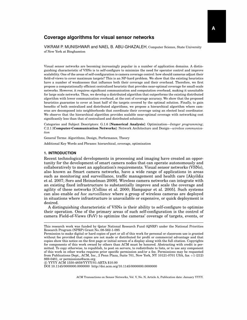
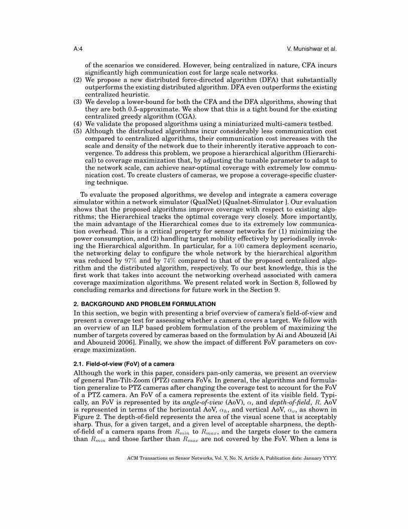
Fig. 1: A general network of wireless Pan cameras. The goal is to maximize the numberof targets covered, where each camera can cover only a spherical sector of limited angle(field-of-view). While Optimal FoV configuration can cover 6 targets, the Greedy FoVselection can cover at most 5 and at least 3 targets, depending on the randomness in thetie-break procedure.
areas of interest. The cameras may be able to change pan, and if available, tilt andzoom to provide the best possible coverage. Since the camera FoVs may overlap withthat of the other cameras, coordination with other cameras is needed to optimize cover-age. As the scale of cameras grows from tens to hundreds of cameras, it is impracticalto rely on human operators to control their setting to achieve the best combined cover-age. Thus, supporting autonomous collaborative coverage is a critical problem in smartcamera networks.
In this paper, we focus on the problem of target coverage maximization; althoughgeneralization to other coverage utility metrics should be straightforward to accom-modate. Specifically, we study the problem of maximizing the number of unique tar-gets covered by all cameras; we call this problem as a Camera Coverage Maximization(CCM) problem. Figure 1 presents a general camera network scenario, with multiplepan-only cameras and a set of targets that need to be monitored. In this example, cam-eras can choose an FoV from 8 discrete FoVs, and their Optimal and Greedy (based onpurely local information) FoV selections are shown in the Figure. While Optimal canmaximize the coverage by covering 6 out of 7 targets (86% coverage), the Greedy policycovers only 5 targets (71% coverage) in the best case and 3 targets (43% coverage) inthe worst case scenario, depending on how the tie-breaks are resolved.
We consider wireless camera networks in our evaluation to further study some of thetradeoffs between delay, messaging overhead and coverage quality in these networks.Although in practice a camera network must track multiple mobile targets in the pres-ence of occlusions, we focus on the problem of coverage of a static set of targets usinga number of pre-deployed cameras as the base step in this direction. Later, these basealgorithms can be adapted to support target mobility.
Our work is most similar to coverage efforts for directional sensor networks. Mosttarget-oriented coverage techniques in this area assume overprovisioned scenarioswhere the sensors can cover all the targets of interest [Soto et al. 2009; Cai et al.2007]. This assumption makes the problem an instance of the set-cover problem, at-tempting to find the optimal configuration to minimize, for example, the number ofsensors needed to cover the targets. In contrast, we consider scenarios where the num-ber of cameras is insufficient to cover the targets, making the problem an instanceof the maximum coverage problem [Hochbaum 1996; Ai and Abouzeid 2006]. Impor-
ACM Transactions on Sensor Networks, Vol. V, No. N, Article A, Publication date: January YYYY.
Coverage Algorithms for Visual Sensor Networks A:3
tantly, the above algorithms consider the coverage problem in isolation, and ignore thenetwork-specific aspects completely. In general, communication overhead, especiallythe delay required to configure all the cameras optimally, can play a significant role inhandling dynamism in the scene effectively. Specifically, when the targets are mobile,optimal camera configurations must be computed and communicated to the respectivecameras quickly before targets move considerably from their recorded positions.
To provide the context for the problem, we first overview an existing Integer LinearProgramming (ILP) formulation of the camera coverage optimization problem devel-oped for directional sensor networks [Ai and Abouzeid 2006]; we modify the existingformulation to account for the different coverage test necessary for camera FoVs. Thisis an NP-hard problem since the decision version of this problem is based on the clas-sical MAX-COVER [Hochbaum 1996], which is NP-complete. The formulation is pre-sented in Section 2.
Due to the high computational complexity of this problem for large-scale networks,polynomial time heuristics are needed. Our work is similar in spirit to the work byAi and Abouzeid [Ai and Abouzeid 2006], who propose greedy heuristics for targetcoverage in directional sensor networks. We show in Section 3 that the existing algo-rithm leads to inefficient solutions even in simple scenarios, primarily because theyonly consider the number of targets, and not the likelihood of a camera making panchoices or the redundancy available to cover a target. In response, we propose newalgorithms that take into account not only the number of new targets covered by acamera, but the likelihood of a camera selecting a particular FoV when it is makingits decision. Thus, in a greedy strategy, our algorithm starts with cameras with moredefinite choices, significantly reducing the likelihood of making bad decisions early. Wealso develop a distributed version of the algorithm in Section 4. We show in Section 5that the proposed centralized and distributed algorithms achieve substantially highercoverage than existing algorithms. In particular, the centralized algorithm tracks op-timal in most cases, while the distributed algorithm outperforms even the existingcentralized algorithm. We also derive approximation bounds for the algorithms andshow that they achieve no worse than 50% of the coverage achieved by the optimalsolution.
Overall, the centralized solutions may be attractive to small-scale networks, as theyprovide high accuracy with acceptable overhead. However, distributed solutions arenecessary for large-scales, where networking overheads and solution time are mini-mized; however they generally lead to a loss in coverage. Moreover, we observed thatdistributed algorithms can require significant convergence time, primarily due to theiriterative nature, which may compromise their agility in highly dynamic scenarios. Toaddress these issues, we propose a hierarchical coverage algorithm where cameras ex-change information within their neighborhoods and coordinate on reaching the bestconfiguration jointly. The neighborhoods are created using a clustering algorithm thatattempts to find clusters of cameras that have significant overlap in their coverage. Weuse a tunable parameter to control the size of the clusters in dense scenarios where it isnot easy to decouple the cameras. The hierarchical algorithm is discussed in Section 6,and evaluated in Section 7.
Summary of Contributions and Findings: This paper proposes a number of newalgorithms for target coverage in smart camera networks. The proposed algorithmsachieve better coverage and scalability than the known algorithms that address thesame problem. The main contributions of this paper can be summarized as below.
(1) We propose a new centralized force-directed algorithm (CFA), which outperformsan existing centralized heuristic, and provides nearly optimal coverage for most
ACM Transactions on Sensor Networks, Vol. V, No. N, Article A, Publication date: January YYYY.
A:4 V. Munishwar et al.
of the scenarios we considered. However, being centralized in nature, CFA incurssignificantly high communication cost for large scale networks.
(2) We propose a new distributed force-directed algorithm (DFA) that substantiallyoutperforms the existing distributed algorithm. DFA even outperforms the existingcentralized heuristic.
(3) We develop a lower-bound for both the CFA and the DFA algorithms, showing thatthey are both 0.5-approximate. We show that this is a tight bound for the existingcentralized greedy algorithm (CGA).
(4) We validate the proposed algorithms using a miniaturized multi-camera testbed.(5) Although the distributed algorithms incur considerably less communication cost
compared to centralized algorithms, their communication cost increases with thescale and density of the network due to their inherently iterative approach to con-vergence. To address this problem, we propose a hierarchical algorithm (Hierarchi-cal) to coverage maximization that, by adjusting the tunable parameter to adapt tothe network scale, can achieve near-optimal coverage with extremely low commu-nication cost. To create clusters of cameras, we propose a coverage-specific cluster-ing technique.
To evaluate the proposed algorithms, we develop and integrate a camera coveragesimulator within a network simulator (QualNet) [Qualnet-Simulator ]. Our evaluationshows that the proposed algorithms improve coverage with respect to existing algo-rithms; the Hierarchical tracks the optimal coverage very closely. More importantly,the main advantage of the Hierarchical comes due to its extremely low communica-tion overhead. This is a critical property for sensor networks for (1) minimizing thepower consumption, and (2) handling target mobility effectively by periodically invok-ing the Hierarchical algorithm. In particular, for a 100 camera deployment scenario,the networking delay to configure the whole network by the hierarchical algorithmwas reduced by 97% and by 74% compared to that of the proposed centralized algo-rithm and the distributed algorithm, respectively. To our best knowledge, this is thefirst work that takes into account the networking overhead associated with cameracoverage maximization algorithms. We present related work in Section 8, followed byconcluding remarks and directions for future work in the Section 9.
2. BACKGROUND AND PROBLEM FORMULATIONIn this section, we begin with presenting a brief overview of camera’s field-of-view andpresent a coverage test for assessing whether a camera covers a target. We follow withan overview of an ILP based problem formulation of the problem of maximizing thenumber of targets covered by cameras based on the formulation by Ai and Abouzeid [Aiand Abouzeid 2006]. Finally, we show the impact of different FoV parameters on cov-erage maximization.
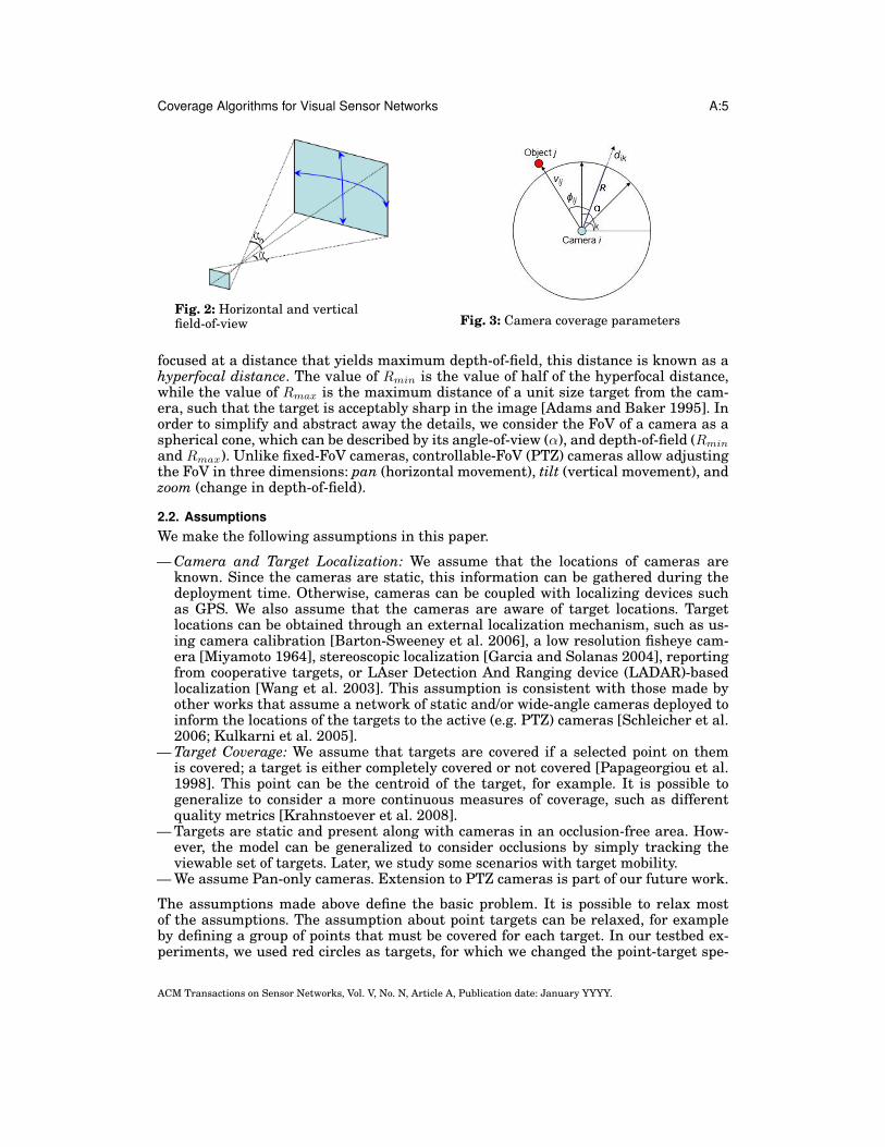
2.1. Field-of-view (FoV) of a cameraAlthough the work in this paper, considers pan-only cameras, we present an overviewof general Pan-Tilt-Zoom (PTZ) camera FoVs. In general, the algorithms and formula-tion generalize to PTZ cameras after changing the coverage test to account for the FoVof a PTZ camera. An FoV of a camera represents the extent of its visible field. Typi-cally, an FoV is represented by its angle-of-view (AoV), α, and depth-of-field, R. AoVis represented in terms of the horizontal AoV, αh, and vertical AoV, αv, as shown inFigure 2. The depth-of-field represents the area of the visual scene that is acceptablysharp. Thus, for a given target, and a given level of acceptable sharpness, the depth-of-field of a camera spans from Rmin to Rmax, and the targets closer to the camerathan Rmin and those farther than Rmax are not covered by the FoV. When a lens is
ACM Transactions on Sensor Networks, Vol. V, No. N, Article A, Publication date: January YYYY.
Coverage Algorithms for Visual Sensor Networks A:5
Fig. 2: Horizontal and verticalfield-of-view Fig. 3: Camera coverage parameters
focused at a distance that yields maximum depth-of-field, this distance is known as ahyperfocal distance. The value of Rmin is the value of half of the hyperfocal distance,while the value of Rmax is the maximum distance of a unit size target from the cam-era, such that the target is acceptably sharp in the image [Adams and Baker 1995]. Inorder to simplify and abstract away the details, we consider the FoV of a camera as aspherical cone, which can be described by its angle-of-view (α), and depth-of-field (Rmin
and Rmax). Unlike fixed-FoV cameras, controllable-FoV (PTZ) cameras allow adjustingthe FoV in three dimensions: pan (horizontal movement), tilt (vertical movement), andzoom (change in depth-of-field).
2.2. AssumptionsWe make the following assumptions in this paper.
— Camera and Target Localization: We assume that the locations of cameras areknown. Since the cameras are static, this information can be gathered during thedeployment time. Otherwise, cameras can be coupled with localizing devices suchas GPS. We also assume that the cameras are aware of target locations. Targetlocations can be obtained through an external localization mechanism, such as us-ing camera calibration [Barton-Sweeney et al. 2006], a low resolution fisheye cam-era [Miyamoto 1964], stereoscopic localization [Garcia and Solanas 2004], reportingfrom cooperative targets, or LAser Detection And Ranging device (LADAR)-basedlocalization [Wang et al. 2003]. This assumption is consistent with those made byother works that assume a network of static and/or wide-angle cameras deployed toinform the locations of the targets to the active (e.g. PTZ) cameras [Schleicher et al.2006; Kulkarni et al. 2005].
— Target Coverage: We assume that targets are covered if a selected point on themis covered; a target is either completely covered or not covered [Papageorgiou et al.1998]. This point can be the centroid of the target, for example. It is possible togeneralize to consider a more continuous measures of coverage, such as differentquality metrics [Krahnstoever et al. 2008].
— Targets are static and present along with cameras in an occlusion-free area. How-ever, the model can be generalized to consider occlusions by simply tracking theviewable set of targets. Later, we study some scenarios with target mobility.
— We assume Pan-only cameras. Extension to PTZ cameras is part of our future work.
The assumptions made above define the basic problem. It is possible to relax mostof the assumptions. The assumption about point targets can be relaxed, for exampleby defining a group of points that must be covered for each target. In our testbed ex-periments, we used red circles as targets, for which we changed the point-target spe-
ACM Transactions on Sensor Networks, Vol. V, No. N, Article A, Publication date: January YYYY.
A:6 V. Munishwar et al.
cific implementation of the coverage test to incorporate targets with given dimensions.Occlusions can also be handled in a number of ways, for example, as part of targetlocalization [Black et al. 2002].
The extension to PTZ cameras is a challenging problem. A primary challenge is thelarge set of FoV settings possible for each camera, which complicates the single cameraassignment and significantly increases the complexity of the multi-camera problem. Aspart of our future work, we plan to develop an algorithm to detect the optimal set ofFoVs for PTZ cameras: most FoVs are either redundant (cover a group of targets iden-tical to other FoVs) or non-maximal (cover a subset of a group targets that are coveredby other FoVs). Once the optimal set of FoVs is derived, the multi-camera problem isidentical to that for the pan-only camera problem: a set of choices are available at ev-ery camera and the optimal assignment of cameras to viable FoVs is attempted by theproblem.
2.3. Preliminaries and NotationFor background, we present a formulation of the problem based on the formulationby Ai and Abouzeid [Ai and Abouzeid 2006]. In particular, we modify the objectivefunction to maximize coverage of a preset group of cameras. In Ai et al.’s formulation,the problem considered also seeks to minimize the number of cameras used in thecoverage.
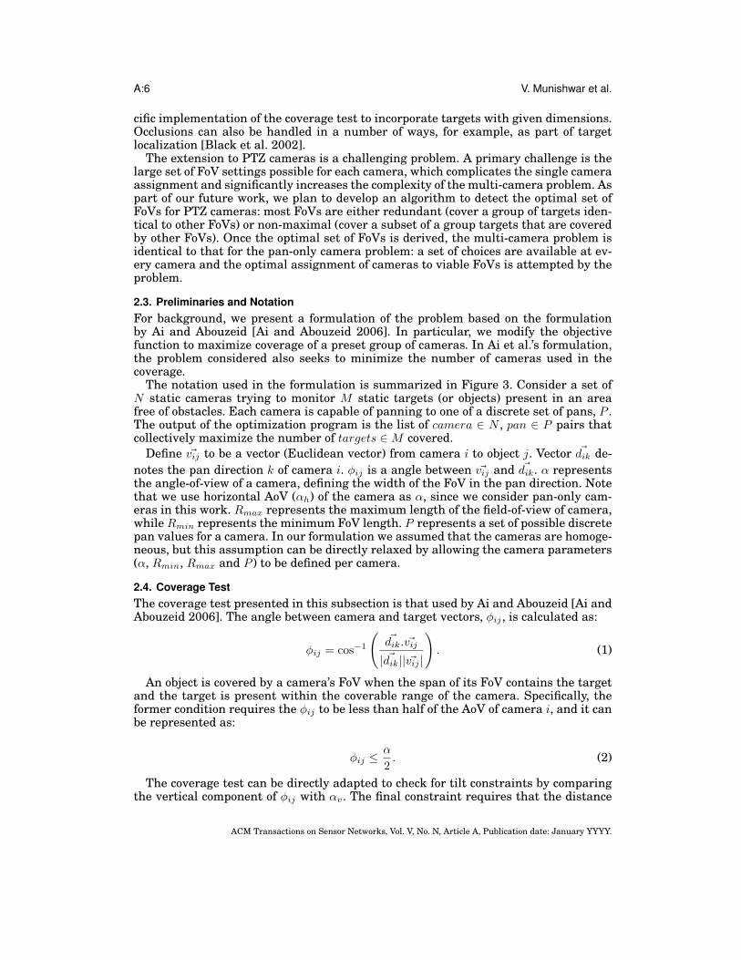
The notation used in the formulation is summarized in Figure 3. Consider a set ofN static cameras trying to monitor M static targets (or objects) present in an areafree of obstacles. Each camera is capable of panning to one of a discrete set of pans, P .The output of the optimization program is the list of camera ∈ N , pan ∈ P pairs thatcollectively maximize the number of targets ∈M covered.
Define ~vij to be a vector (Euclidean vector) from camera i to object j. Vector ~dik de-notes the pan direction k of camera i. φij is a angle between ~vij and ~dik. α representsthe angle-of-view of a camera, defining the width of the FoV in the pan direction. Notethat we use horizontal AoV (αh) of the camera as α, since we consider pan-only cam-eras in this work. Rmax represents the maximum length of the field-of-view of camera,while Rmin represents the minimum FoV length. P represents a set of possible discretepan values for a camera. In our formulation we assumed that the cameras are homoge-neous, but this assumption can be directly relaxed by allowing the camera parameters(α, Rmin, Rmax and P ) to be defined per camera.
2.4. Coverage TestThe coverage test presented in this subsection is that used by Ai and Abouzeid [Ai andAbouzeid 2006]. The angle between camera and target vectors, φij , is calculated as:
φij = cos−1
(~dik. ~vij
| ~dik|| ~vij |
). (1)
An object is covered by a camera’s FoV when the span of its FoV contains the targetand the target is present within the coverable range of the camera. Specifically, theformer condition requires the φij to be less than half of the AoV of camera i, and it canbe represented as:
φij ≤α
2. (2)
The coverage test can be directly adapted to check for tilt constraints by comparingthe vertical component of φij with αv. The final constraint requires that the distance
ACM Transactions on Sensor Networks, Vol. V, No. N, Article A, Publication date: January YYYY.
Coverage Algorithms for Visual Sensor Networks A:7
between the camera and the target is within Rmin and Rmax, and can be representedas:
Rmin ≤ | ~vij | ≤ Rmax. (3)
Using the above coverage test, each camera can generate its coverage matrix AMN×P
such that each element of the matrix, ajik, represents whether the camera i can coverobject j with pan k.
ajik =
{1 if camera i with pan k covers object j.0 otherwise.
2.5. ILP Formulation of the CCM ProblemThe utility (or importance) of the targets is assumed to be equal. Thus, the primeobjective is to maximize the overall number of covered targets. A target covered bymultiple cameras only counts as one target towards the overall objective.
Maximize∑j∈M
γj . (4)
Where, γj is a binary variable that takes value 1 when target j is covered by at leastone camera, and 0 otherwise. Coverage is determined by the coverage test described inthe previous subsection.
The constraints of the problem can be represented as:∑k∈P
Xik ≤ 1 ∀i ∈ N. (5)
∑i∈N,k∈P a
jikXik
L≤ γj ≤
∑i∈N,k∈P
ajikXik ∀j ∈M. (6)
X ∈ {0, 1} , γ ∈ {0, 1} . (7)Equation 5 represents that a camera can choose only one pan at a time, where Xik
is a binary variable which takes value 1 if pan k is selected for camera i. Equation 6ensures that the utility γj for target j can be at most 1, irrespective of the numberof cameras covering that target. Here, L is an arbitrary large value (L ≥ ‖N‖). Thus,γj can assign itself a value 1 if target j is covered by at least one camera, and 0 oth-erwise. CCM is an Integer Linear Programming (ILP) problem and it is shown to beNP-hard [Ai and Abouzeid 2006].
Since the CCM problem is NP-hard [Ai and Abouzeid 2006], in Section 3, we presenta polynomial-time, near-optimal, heuristic.
2.6. Discussion and ObservationsCoverage maximization for camera networks becomes difficult when either: (1) thenumber of possible FoVs a camera can take increases; and (2) the inter-dependenceamong cameras (i.e., overlap in the objects they cover) increases. The former conditionoccurs when the angle-of-view (AoV) decreases, resulting in increased number of non-overlapped discrete FoVs 1. The latter condition occurs when the depth-of-field (FoV
1Another way is to consider overlapped discrete FoVs with smaller step size.
ACM Transactions on Sensor Networks, Vol. V, No. N, Article A, Publication date: January YYYY.
A:8 V. Munishwar et al.
A45 A180 A3600
20
40
60
80
100
Angle of View (degrees)
Perc
ent C
overa
ge
Optimal
Greedy
Fig. 4: Impact of different angle-of-views(AoVs)
R20 R60 R1000
10
20
30
40
50
60
70
80
90
FoV Range (meters)
Perc
ent C
overa
ge
Optimal
Greedy
Fig. 5: Impact of different FoV ranges
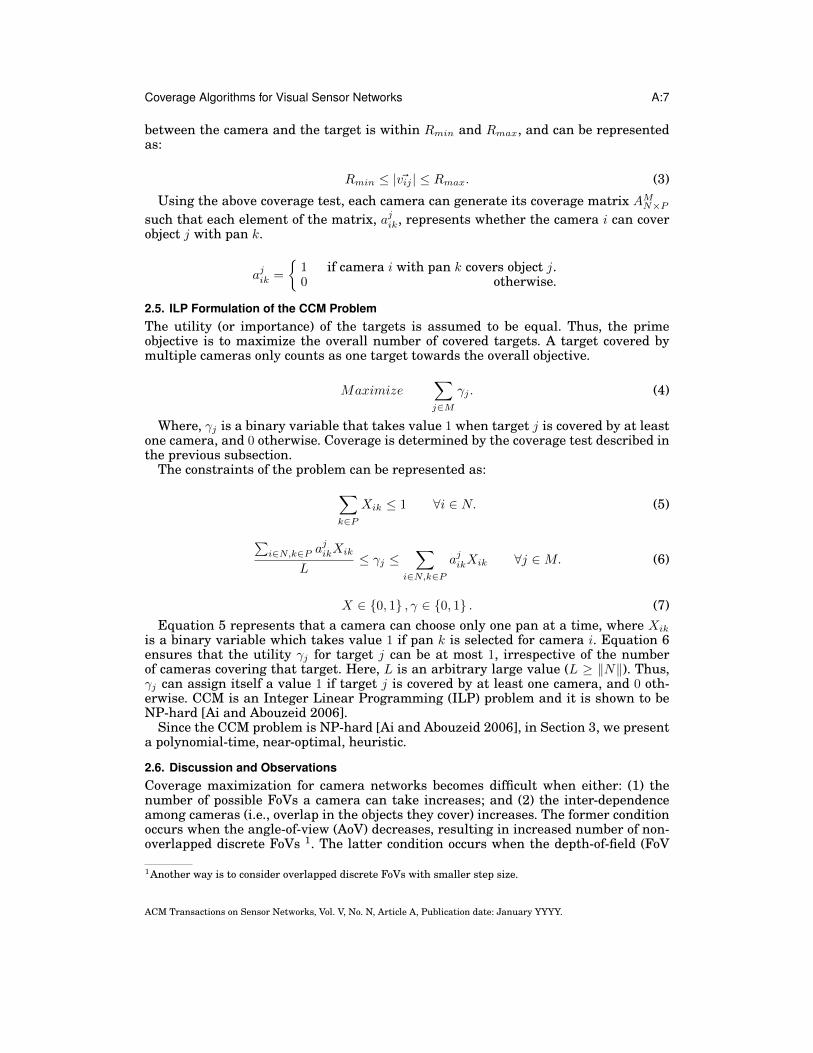
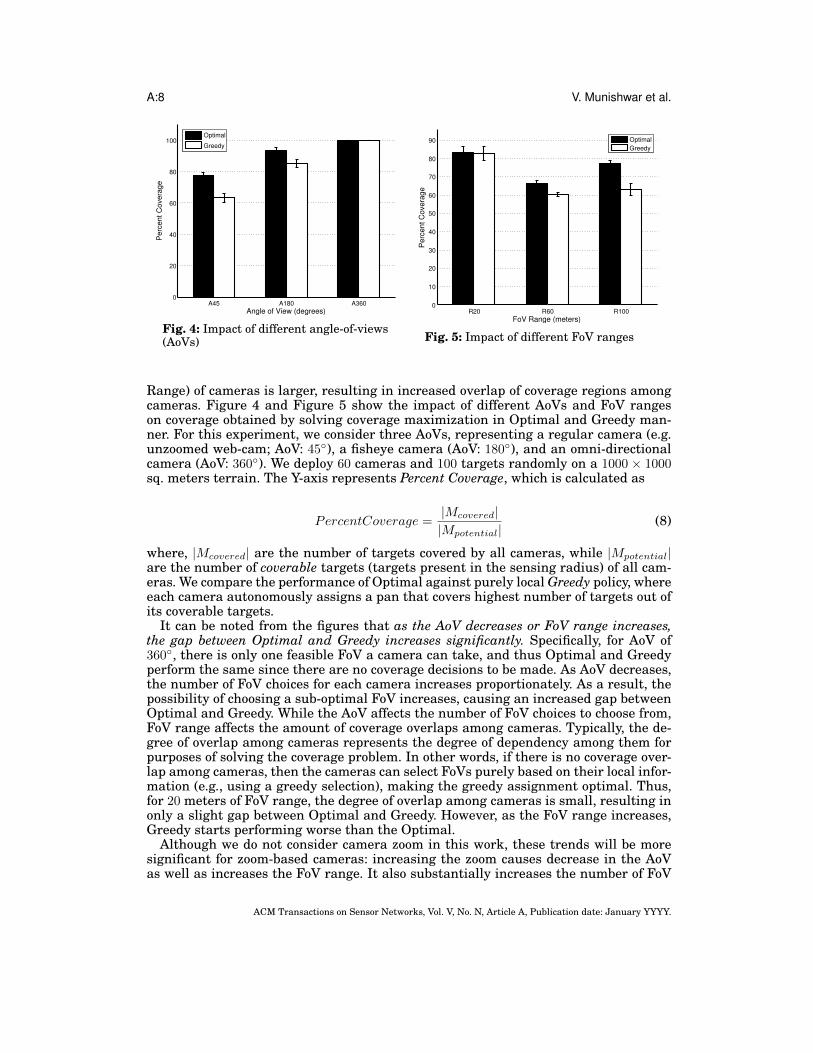
Range) of cameras is larger, resulting in increased overlap of coverage regions amongcameras. Figure 4 and Figure 5 show the impact of different AoVs and FoV rangeson coverage obtained by solving coverage maximization in Optimal and Greedy man-ner. For this experiment, we consider three AoVs, representing a regular camera (e.g.unzoomed web-cam; AoV: 45◦), a fisheye camera (AoV: 180◦), and an omni-directionalcamera (AoV: 360◦). We deploy 60 cameras and 100 targets randomly on a 1000 × 1000sq. meters terrain. The Y-axis represents Percent Coverage, which is calculated as
PercentCoverage =|Mcovered||Mpotential|
(8)
where, |Mcovered| are the number of targets covered by all cameras, while |Mpotential|are the number of coverable targets (targets present in the sensing radius) of all cam-eras. We compare the performance of Optimal against purely local Greedy policy, whereeach camera autonomously assigns a pan that covers highest number of targets out ofits coverable targets.
It can be noted from the figures that as the AoV decreases or FoV range increases,the gap between Optimal and Greedy increases significantly. Specifically, for AoV of360◦, there is only one feasible FoV a camera can take, and thus Optimal and Greedyperform the same since there are no coverage decisions to be made. As AoV decreases,the number of FoV choices for each camera increases proportionately. As a result, thepossibility of choosing a sub-optimal FoV increases, causing an increased gap betweenOptimal and Greedy. While the AoV affects the number of FoV choices to choose from,FoV range affects the amount of coverage overlaps among cameras. Typically, the de-gree of overlap among cameras represents the degree of dependency among them forpurposes of solving the coverage problem. In other words, if there is no coverage over-lap among cameras, then the cameras can select FoVs purely based on their local infor-mation (e.g., using a greedy selection), making the greedy assignment optimal. Thus,for 20 meters of FoV range, the degree of overlap among cameras is small, resulting inonly a slight gap between Optimal and Greedy. However, as the FoV range increases,Greedy starts performing worse than the Optimal.
Although we do not consider camera zoom in this work, these trends will be moresignificant for zoom-based cameras: increasing the zoom causes decrease in the AoVas well as increases the FoV range. It also substantially increases the number of FoV
ACM Transactions on Sensor Networks, Vol. V, No. N, Article A, Publication date: January YYYY.
Coverage Algorithms for Visual Sensor Networks A:9
Fig. 6: Dependence ofCGA on cameraselection order
Fig. 7: Dependence ofCGA on pan selectionorder Fig. 8: A counter
example for CGA
choices available for each camera. Thus, it is important to explore heuristics that arebetter than greedy, but that perform more efficiently than optimal.
3. CENTRALIZED FORCE-DIRECTED ALGORITHM (CFA)Since the optimal problem is NP-hard, it becomes impractical to solve it optimally asthe number of cameras and the number of feasible FoVs per camera both increase.Thus, it is necessary to develop heuristics that perform close to optimal. In this sec-tion, we first describe the existing state-of-the-art algorithm and analyze some basiccases where it fails to provide optimal configurations. We then present the proposedCentralized Force-based Algorithm (CFA). We also derive an approximation bound forboth the existing and the new algorithm.
3.1. Existing solution: Centralized Greedy Algorithm (CGA)The Centralized Greedy Algorithm (CGA) [Ai and Abouzeid 2006] was proposed in thecontext of directional sensor networks. CGA begins with making all cameras inactive.In each iteration, it selects the inactive camera that can cover the maximum numberof uncovered objects using a single pan direction. Cameras that have been selectedalready and their covered targets are not considered in successive iterations. The al-gorithm terminates when all the cameras are assigned a direction.
CGA can lead to a number of basic cases with suboptimal camera-pan configurations.These patterns arise commonly within camera networks.
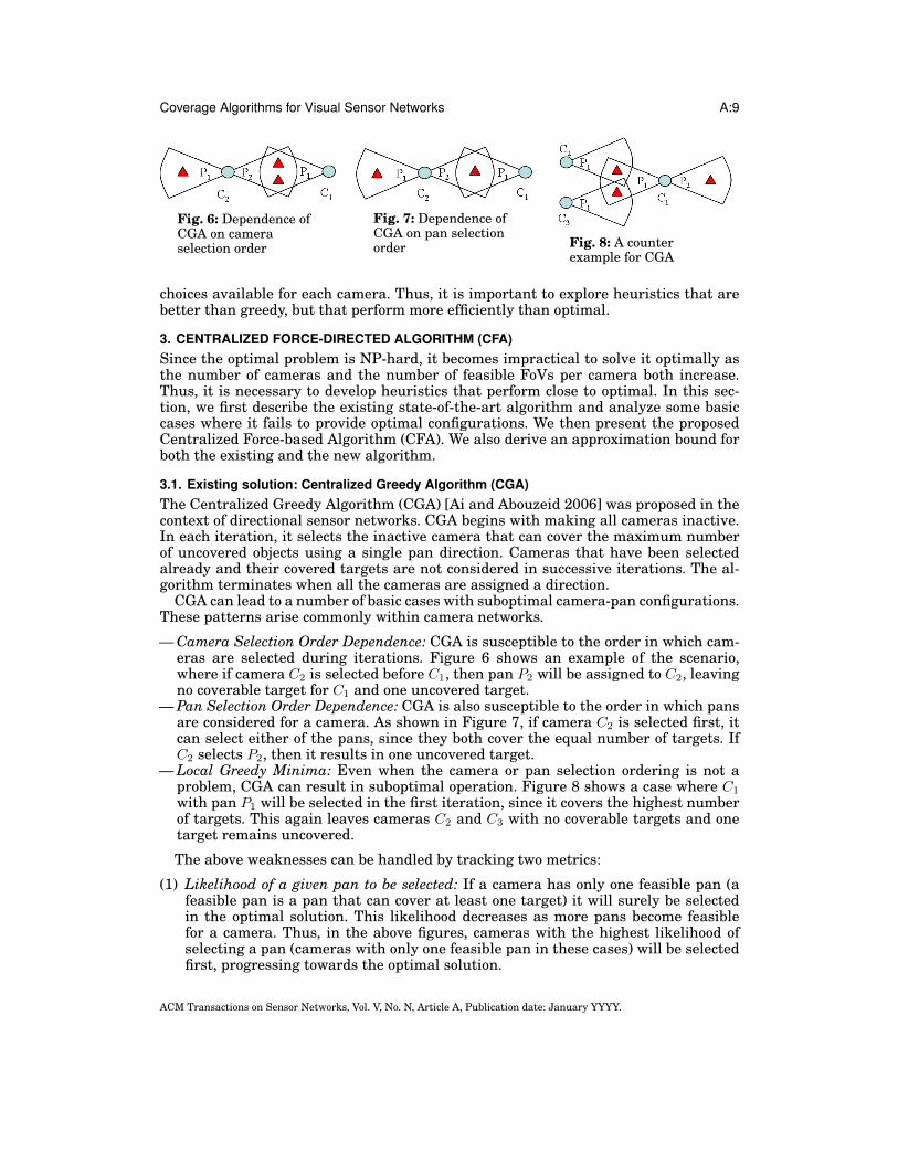
— Camera Selection Order Dependence: CGA is susceptible to the order in which cam-eras are selected during iterations. Figure 6 shows an example of the scenario,where if camera C2 is selected before C1, then pan P2 will be assigned to C2, leavingno coverable target for C1 and one uncovered target.
— Pan Selection Order Dependence: CGA is also susceptible to the order in which pansare considered for a camera. As shown in Figure 7, if camera C2 is selected first, itcan select either of the pans, since they both cover the equal number of targets. IfC2 selects P2, then it results in one uncovered target.
— Local Greedy Minima: Even when the camera or pan selection ordering is not aproblem, CGA can result in suboptimal operation. Figure 8 shows a case where C1
with pan P1 will be selected in the first iteration, since it covers the highest numberof targets. This again leaves cameras C2 and C3 with no coverable targets and onetarget remains uncovered.
The above weaknesses can be handled by tracking two metrics:
(1) Likelihood of a given pan to be selected: If a camera has only one feasible pan (afeasible pan is a pan that can cover at least one target) it will surely be selectedin the optimal solution. This likelihood decreases as more pans become feasiblefor a camera. Thus, in the above figures, cameras with the highest likelihood ofselecting a pan (cameras with only one feasible pan in these cases) will be selectedfirst, progressing towards the optimal solution.
ACM Transactions on Sensor Networks, Vol. V, No. N, Article A, Publication date: January YYYY.
A:10 V. Munishwar et al.
Fig. 9: Illustration of Force-directed Algorithm
(a) (b) (c)
Fig. 10: Counter example for CFA. (a) Scenario where CFA does not produce optimalconfigurations. (b) Optimal configurations (c) Configurations generated by CFA
(2) Coverability of a target: A target is considered to be difficult to cover if it is coverableby fewer cameras, and vice versa. Thus, more preference is given to the targets thatare difficult to cover. In the above figures, targets that can be covered by the leastnumber of cameras will be covered first, reaching the optimal solution.
While the first algorithm needs only local information available at a camera, thesecond algorithm needs the coverage information from all the cameras that can covera given target. Thus, we use the first algorithm for our proposed algorithm since it isbetter suited for distributed implementations.
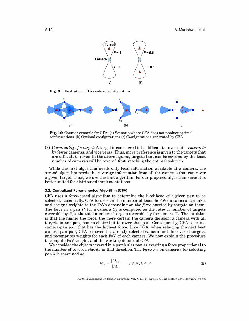
3.2. Centralized Force-directed Algorithm (CFA)CFA uses a force-based algorithm to determine the likelihood of a given pan to beselected. Essentially, CFA focuses on the number of feasible FoVs a camera can take,and assigns weights to the FoVs depending on the force exerted by targets on them.The force in a pan Pi for a camera Cj is computed as the ratio of number of targetscoverable by Pi to the total number of targets coverable by the camera Cj . The intuitionis that the higher the force, the more certain the camera decision: a camera with alltargets in one pan, has no choice but to cover that pan. Consequently, CFA selects acamera-pan pair that has the highest force. Like CGA, when selecting the next bestcamera-pan pair, CFA removes the already selected camera and its covered targets,and recomputes weights for each FoV of each camera. We now explain the procedureto compute FoV weight, and the working details of CFA.
We consider the objects covered in a particular pan as exerting a force proportional tothe number of covered objects in that direction. The force Fik on camera i for selectingpan k is computed as:
Fik =|Mik||Mi|
i ∈ N, k ∈ P (9)
ACM Transactions on Sensor Networks, Vol. V, No. N, Article A, Publication date: January YYYY.
Coverage Algorithms for Visual Sensor Networks A:11
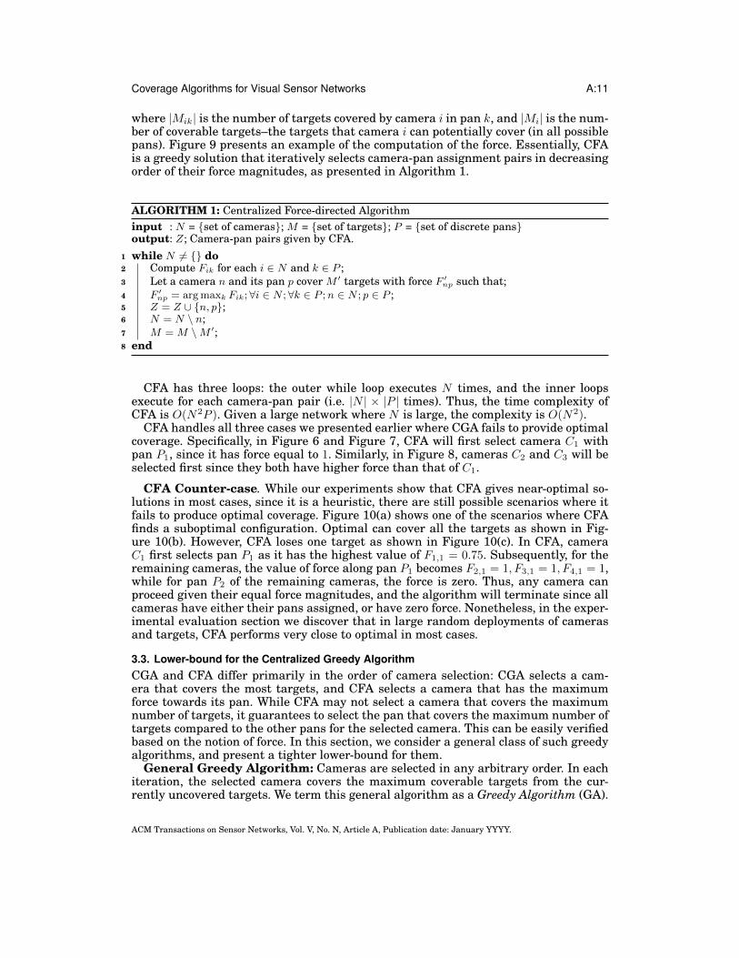
where |Mik| is the number of targets covered by camera i in pan k, and |Mi| is the num-ber of coverable targets–the targets that camera i can potentially cover (in all possiblepans). Figure 9 presents an example of the computation of the force. Essentially, CFAis a greedy solution that iteratively selects camera-pan assignment pairs in decreasingorder of their force magnitudes, as presented in Algorithm 1.
ALGORITHM 1: Centralized Force-directed Algorithminput : N = {set of cameras}; M = {set of targets}; P = {set of discrete pans}output: Z; Camera-pan pairs given by CFA.
1 while N 6= {} do2 Compute Fik for each i ∈ N and k ∈ P ;3 Let a camera n and its pan p cover M ′ targets with force F ′
np such that;4 F ′
np = arg maxk Fik; ∀i ∈ N ;∀k ∈ P ;n ∈ N ; p ∈ P ;5 Z = Z ∪ {n, p};6 N = N \ n;7 M = M \M ′;8 end
CFA has three loops: the outer while loop executes N times, and the inner loopsexecute for each camera-pan pair (i.e. |N | × |P | times). Thus, the time complexity ofCFA is O(N2P ). Given a large network where N is large, the complexity is O(N2).
CFA handles all three cases we presented earlier where CGA fails to provide optimalcoverage. Specifically, in Figure 6 and Figure 7, CFA will first select camera C1 withpan P1, since it has force equal to 1. Similarly, in Figure 8, cameras C2 and C3 will beselected first since they both have higher force than that of C1.
CFA Counter-case. While our experiments show that CFA gives near-optimal so-lutions in most cases, since it is a heuristic, there are still possible scenarios where itfails to produce optimal coverage. Figure 10(a) shows one of the scenarios where CFAfinds a suboptimal configuration. Optimal can cover all the targets as shown in Fig-ure 10(b). However, CFA loses one target as shown in Figure 10(c). In CFA, cameraC1 first selects pan P1 as it has the highest value of F1,1 = 0.75. Subsequently, for theremaining cameras, the value of force along pan P1 becomes F2,1 = 1, F3,1 = 1, F4,1 = 1,while for pan P2 of the remaining cameras, the force is zero. Thus, any camera canproceed given their equal force magnitudes, and the algorithm will terminate since allcameras have either their pans assigned, or have zero force. Nonetheless, in the exper-imental evaluation section we discover that in large random deployments of camerasand targets, CFA performs very close to optimal in most cases.
3.3. Lower-bound for the Centralized Greedy AlgorithmCGA and CFA differ primarily in the order of camera selection: CGA selects a cam-era that covers the most targets, and CFA selects a camera that has the maximumforce towards its pan. While CFA may not select a camera that covers the maximumnumber of targets, it guarantees to select the pan that covers the maximum number oftargets compared to the other pans for the selected camera. This can be easily verifiedbased on the notion of force. In this section, we consider a general class of such greedyalgorithms, and present a tighter lower-bound for them.
General Greedy Algorithm: Cameras are selected in any arbitrary order. In eachiteration, the selected camera covers the maximum coverable targets from the cur-rently uncovered targets. We term this general algorithm as a Greedy Algorithm (GA).
ACM Transactions on Sensor Networks, Vol. V, No. N, Article A, Publication date: January YYYY.
A:12 V. Munishwar et al.
Once a camera is selected, both CGA and CFA configure it in a greedy way: theyselect the pan that covers the maximum number of targets. The algorithms differ onlyin the order of selection of cameras to configure. Since the general greedy algorithmadmits arbitrary order of camera selection, both CGA and CFA represent special casesof the general greedy algorithm. We show that both GA (and therefore both CGA andCFA) have an approximation bound of 0.5.
We use the following notation. Consider a scenario S0 with N cameras and M cover-able targets. Let m(Cg
i ) and m(Coi ) represent the number of targets covered by camera
i ∈ N following the Greedy Algorithm (GA) and the Optimal Algorithm (OA), respec-tively. Let M(Co
i ) and M(Cgi ) denote the set of targets covered by camera i using OA
and GA, respectively. OA covers a total of mo targets, and GA covers a total mg targets.
THEOREM 3.1. mg ≥ 12m
o.
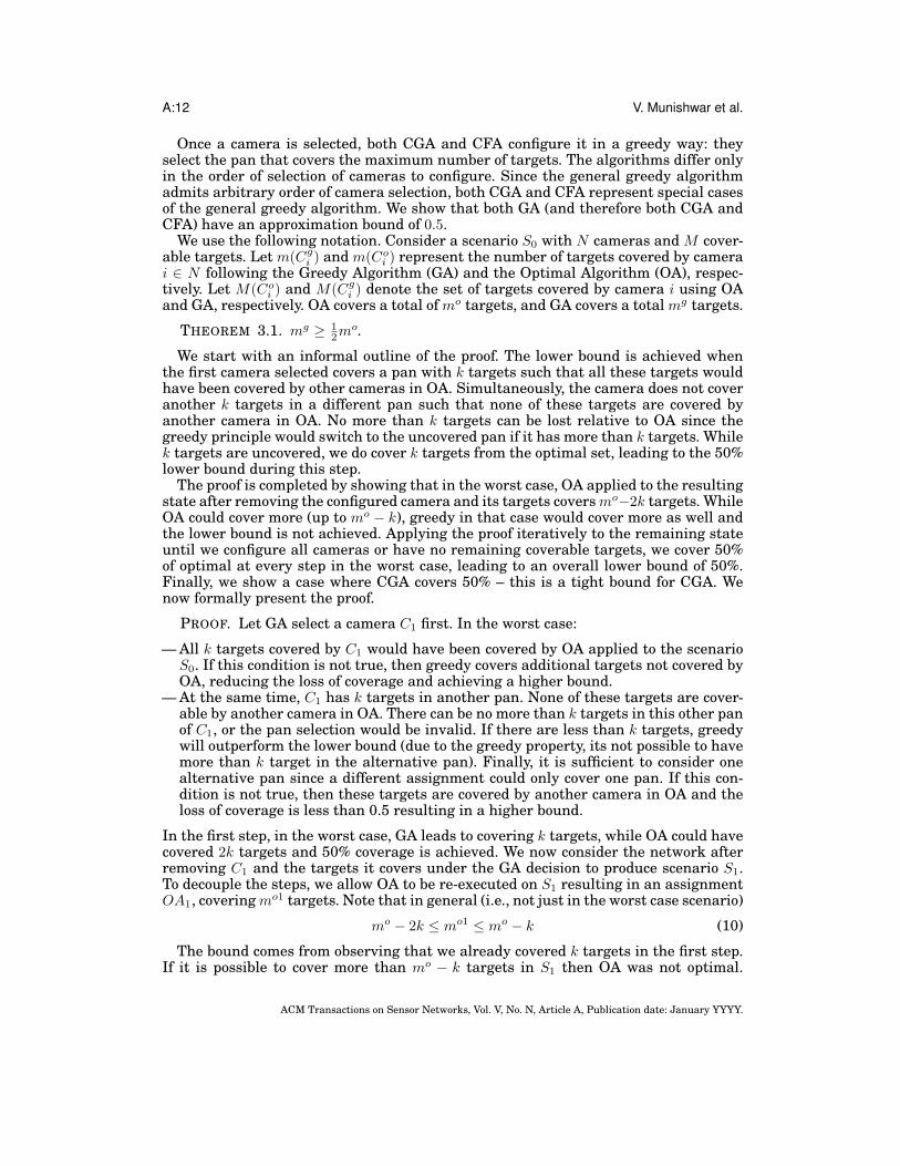
We start with an informal outline of the proof. The lower bound is achieved whenthe first camera selected covers a pan with k targets such that all these targets wouldhave been covered by other cameras in OA. Simultaneously, the camera does not coveranother k targets in a different pan such that none of these targets are covered byanother camera in OA. No more than k targets can be lost relative to OA since thegreedy principle would switch to the uncovered pan if it has more than k targets. Whilek targets are uncovered, we do cover k targets from the optimal set, leading to the 50%lower bound during this step.
The proof is completed by showing that in the worst case, OA applied to the resultingstate after removing the configured camera and its targets coversmo−2k targets. WhileOA could cover more (up to mo − k), greedy in that case would cover more as well andthe lower bound is not achieved. Applying the proof iteratively to the remaining stateuntil we configure all cameras or have no remaining coverable targets, we cover 50%of optimal at every step in the worst case, leading to an overall lower bound of 50%.Finally, we show a case where CGA covers 50% – this is a tight bound for CGA. Wenow formally present the proof.
PROOF. Let GA select a camera C1 first. In the worst case:
— All k targets covered by C1 would have been covered by OA applied to the scenarioS0. If this condition is not true, then greedy covers additional targets not covered byOA, reducing the loss of coverage and achieving a higher bound.
— At the same time, C1 has k targets in another pan. None of these targets are cover-able by another camera in OA. There can be no more than k targets in this other panof C1, or the pan selection would be invalid. If there are less than k targets, greedywill outperform the lower bound (due to the greedy property, its not possible to havemore than k target in the alternative pan). Finally, it is sufficient to consider onealternative pan since a different assignment could only cover one pan. If this con-dition is not true, then these targets are covered by another camera in OA and theloss of coverage is less than 0.5 resulting in a higher bound.
In the first step, in the worst case, GA leads to covering k targets, while OA could havecovered 2k targets and 50% coverage is achieved. We now consider the network afterremoving C1 and the targets it covers under the GA decision to produce scenario S1.To decouple the steps, we allow OA to be re-executed on S1 resulting in an assignmentOA1, coveringmo1 targets. Note that in general (i.e., not just in the worst case scenario)
mo − 2k ≤ mo1 ≤ mo − k (10)
The bound comes from observing that we already covered k targets in the first step.If it is possible to cover more than mo − k targets in S1 then OA was not optimal.
ACM Transactions on Sensor Networks, Vol. V, No. N, Article A, Publication date: January YYYY.
Coverage Algorithms for Visual Sensor Networks A:13
The lower bound occurs when all targets covered by the GA with C1 could have beencovered by OA1, and none of the targets that are not covered in the alternative panfor C1 can be covered by OA1. This represents a lower bound on mo1 since no otherdecision on C1 could lead to covering more than an additional k targets.
Note that by allowing OA to be reexecuted at every step, the steps are decoupled.The same reasoning can now be applied to S1 to show that the next camera selected inGA can lead to no worse than 50% of OA1.
For deriving the lower bound it is sufficient to consider the lower bound on mo1.Since the steps are decoupled, if more than the lower bound is coverable by OA1 thenthe proof shows that no less than 50% of this new and higher bound is coverable by GA.Thus, the overall coverage of GA will be more than 50% of the original OA assignmentapplied to S0.
To get the bound, in the worst case,OA1 coversmo−2k. We apply the same reasoningfor the next camera selection and do so recursively until all cameras are assigned orno more coverable targets exist. At every step, GA in the worst case achieves 50%coverage of OA, leading to an overall GA approximation bound of 50%.
Since GA yields a 0.5-approximate solution, both CGA and CFA, which are specialcases of GA, also provide a 0.5-approximate solution to the CCM problem.
We now show the minimal example where CGA achieves exactly half of the coverageof optimal, showing that 0.5 is a tight bound. Consider a scenario with 2 cameras C1
and C2 as shown in Figure 7. C2 has one target t1 coverable in pan P1 and anothert2 coverable in pan P2. C1 can cover only t2 in pan P1. The optimal solution coversboth targets by configuring C1 to cover t2 and C2 to cover t1. However, if greedy pickscamera C2 to assign first, and assigns it to pan P2, C1 has no targets to cover, and onlyone target is covered. Note that this is our worst case scenario where C2 picks a panwhere the target would have been covered by OA and there exists another pan wherethe target could not have been covered otherwise by OA. It is interesting to note thatCFA achieves optimal assignment for this scenario. We were not able to come up witha scenario where CFA achieves 0.5 coverage, so there is a possibility that there existsa tighter bound than 0.5 for it.
4. DISTRIBUTED COVERAGE MAXIMIZATION PROTOCOLIn this section, we first describe the state-of-the-art distributed algorithm for coveragemaximization in the context of directional sensor networks, followed by our proposeddistributed algorithm.
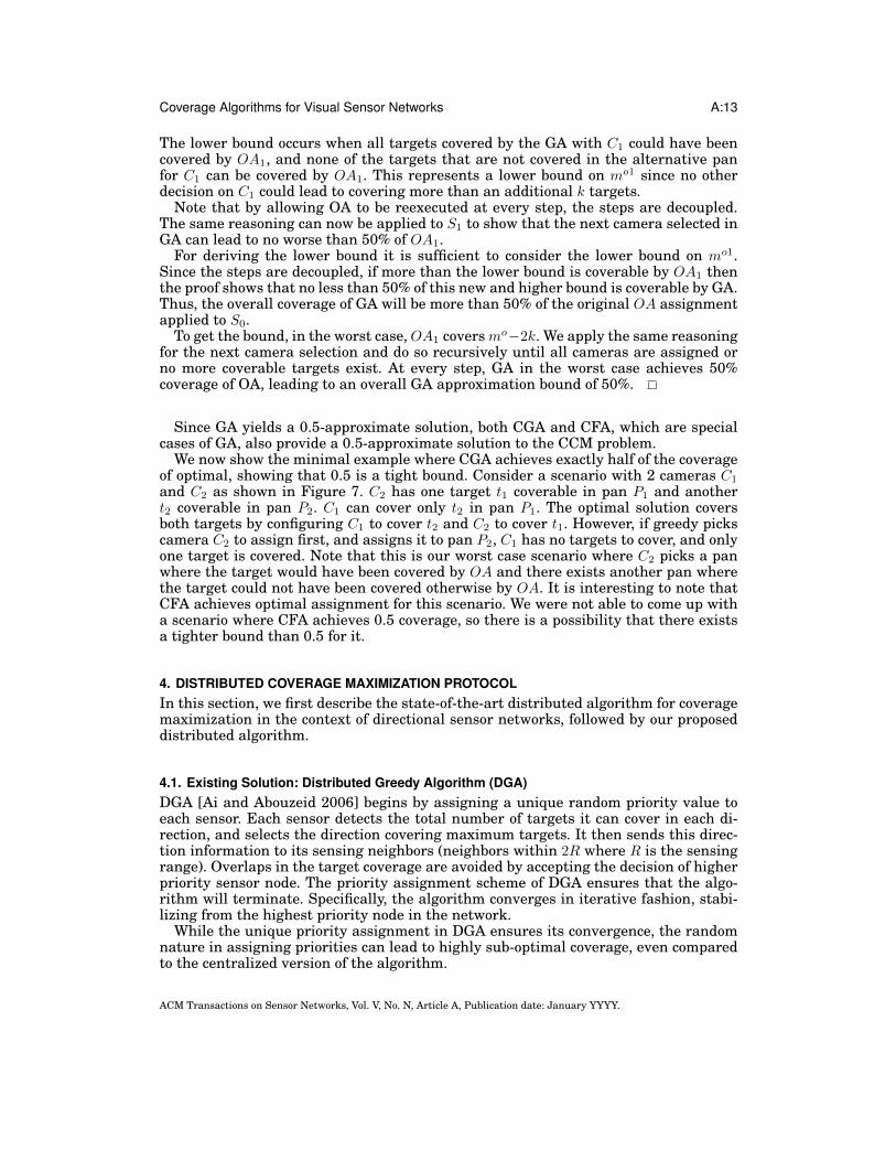
4.1. Existing Solution: Distributed Greedy Algorithm (DGA)DGA [Ai and Abouzeid 2006] begins by assigning a unique random priority value toeach sensor. Each sensor detects the total number of targets it can cover in each di-rection, and selects the direction covering maximum targets. It then sends this direc-tion information to its sensing neighbors (neighbors within 2R where R is the sensingrange). Overlaps in the target coverage are avoided by accepting the decision of higherpriority sensor node. The priority assignment scheme of DGA ensures that the algo-rithm will terminate. Specifically, the algorithm converges in iterative fashion, stabi-lizing from the highest priority node in the network.
While the unique priority assignment in DGA ensures its convergence, the randomnature in assigning priorities can lead to highly sub-optimal coverage, even comparedto the centralized version of the algorithm.
ACM Transactions on Sensor Networks, Vol. V, No. N, Article A, Publication date: January YYYY.
A:14 V. Munishwar et al.
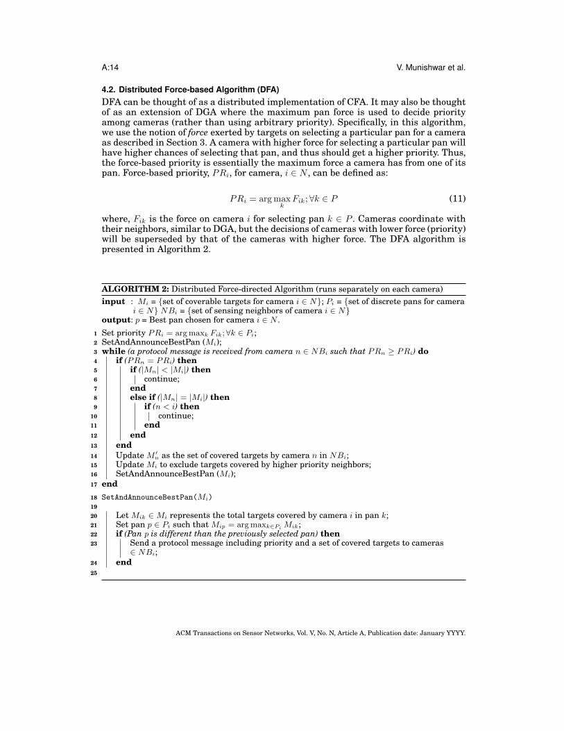
4.2. Distributed Force-based Algorithm (DFA)DFA can be thought of as a distributed implementation of CFA. It may also be thoughtof as an extension of DGA where the maximum pan force is used to decide priorityamong cameras (rather than using arbitrary priority). Specifically, in this algorithm,we use the notion of force exerted by targets on selecting a particular pan for a cameraas described in Section 3. A camera with higher force for selecting a particular pan willhave higher chances of selecting that pan, and thus should get a higher priority. Thus,the force-based priority is essentially the maximum force a camera has from one of itspan. Force-based priority, PRi, for camera, i ∈ N , can be defined as:
PRi = argmaxk
Fik;∀k ∈ P (11)
where, Fik is the force on camera i for selecting pan k ∈ P . Cameras coordinate withtheir neighbors, similar to DGA, but the decisions of cameras with lower force (priority)will be superseded by that of the cameras with higher force. The DFA algorithm ispresented in Algorithm 2.
ALGORITHM 2: Distributed Force-directed Algorithm (runs separately on each camera)input : Mi = {set of coverable targets for camera i ∈ N}; Pi = {set of discrete pans for camera
i ∈ N} NBi = {set of sensing neighbors of camera i ∈ N}output: p = Best pan chosen for camera i ∈ N .
1 Set priority PRi = arg maxk Fik; ∀k ∈ Pi;2 SetAndAnnounceBestPan (Mi);3 while (a protocol message is received from camera n ∈ NBi such that PRn ≥ PRi) do4 if (PRn = PRi) then5 if (|Mn| < |Mi|) then6 continue;7 end8 else if (|Mn| = |Mi|) then9 if (n < i) then
10 continue;11 end12 end13 end14 Update M ′
n as the set of covered targets by camera n in NBi;15 Update Mi to exclude targets covered by higher priority neighbors;16 SetAndAnnounceBestPan (Mi);17 end18 SetAndAnnounceBestPan(Mi)1920 Let Mik ∈Mi represents the total targets covered by camera i in pan k;21 Set pan p ∈ Pi such that Mip = arg maxk∈Pi Mik;22 if (Pan p is different than the previously selected pan) then23 Send a protocol message including priority and a set of covered targets to cameras
∈ NBi;24 end25
ACM Transactions on Sensor Networks, Vol. V, No. N, Article A, Publication date: January YYYY.
Coverage Algorithms for Visual Sensor Networks A:15
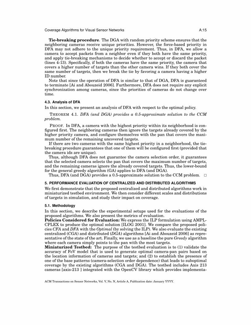
Tie-breaking procedure. The DGA with random priority scheme ensures that theneighboring cameras receive unique priorities. However, the force-based priority inDFA may not adhere to the unique priority requirement. Thus, in DFA, we allow acamera to accept packets from a neighbor even if they both have the same priority,and apply tie-breaking mechanisms to decide whether to accept or discard the packet(lines 4-13). Specifically, if both the cameras have the same priority, the camera thatcovers a higher number of targets than the other camera wins. If they both cover thesame number of targets, then we break the tie by favoring a camera having a higherID number.
Note that since the operation of DFA is similar to that of DGA, DFA is guaranteedto terminate [Ai and Abouzeid 2006]. Furthermore, DFA does not require any explicitsynchronization among cameras, since the priorities of cameras do not change overtime.
4.3. Analysis of DFAIn this section, we present an analysis of DFA with respect to the optimal policy.
THEOREM 4.1. DFA (and DGA) provides a 0.5-approximate solution to the CCMproblem.
PROOF. In DFA, a camera with the highest priority within its neighborhood is con-figured first. The neighboring cameras then ignore the targets already covered by thehigher priority camera, and configure themselves with the pan that covers the maxi-mum number of the remaining uncovered targets.
If there are two cameras with the same highest priority in a neighborhood, the tie-breaking procedure guarantees that one of them will be configured first (provided thatthe camera ids are unique).
Thus, although DFA does not guarantee the camera selection order, it guaranteesthat the selected camera selects the pan that covers the maximum number of targets,and the remaining cameras ignore the already covered targets. Thus, the lower-boundfor the general greedy algorithm (GA) applies to DFA (and DGA).
Thus, DFA (and DGA) provides a 0.5-approximate solution to the CCM problem.
5. PERFORMANCE EVALUATION OF CENTRALIZED AND DISTRIBUTED ALGORITHMSWe first demonstrate that the proposed centralized and distributed algorithms work inminiaturized testbed environment. We then consider different scales and distributionsof targets in simulation, and study their impact on coverage.
5.1. MethodologyIn this section, we describe the experimental setups used for the evaluations of theproposed algorithms. We also present the metrics of evaluation.Policies Considered for Evaluation: We express the ILP formulation using AMPL-CPLEX to produce the optimal solution [ILOG 2001]. We compare the proposed poli-cies CFA and DFA with the Optimal (by solving the ILP). We also evaluate the existingcentralized (CGA) and distributed (DGA) algorithms [Ai and Abouzeid 2006] as repre-sentative of the state of the art. Finally, we use as a baseline the pure Greedy algorithmwhere each camera simply points to the pan with the most targets.Miniaturized Testbed: The purpose of the testbed evaluation is to (1) validate theaccuracy of FoV model that is used to generate optimal camera-pan pairs based onthe location information of cameras and targets; and (2) to establish the presence ofone of the base patterns (camera-selection order dependence) that leads to suboptimalcoverage by the existing algorithms (CGA and DGA). The testbed includes Axis 213cameras [axis-213 ] integrated with the OpenCV library which provides implementa-
ACM Transactions on Sensor Networks, Vol. V, No. N, Article A, Publication date: January YYYY.
A:16 V. Munishwar et al.
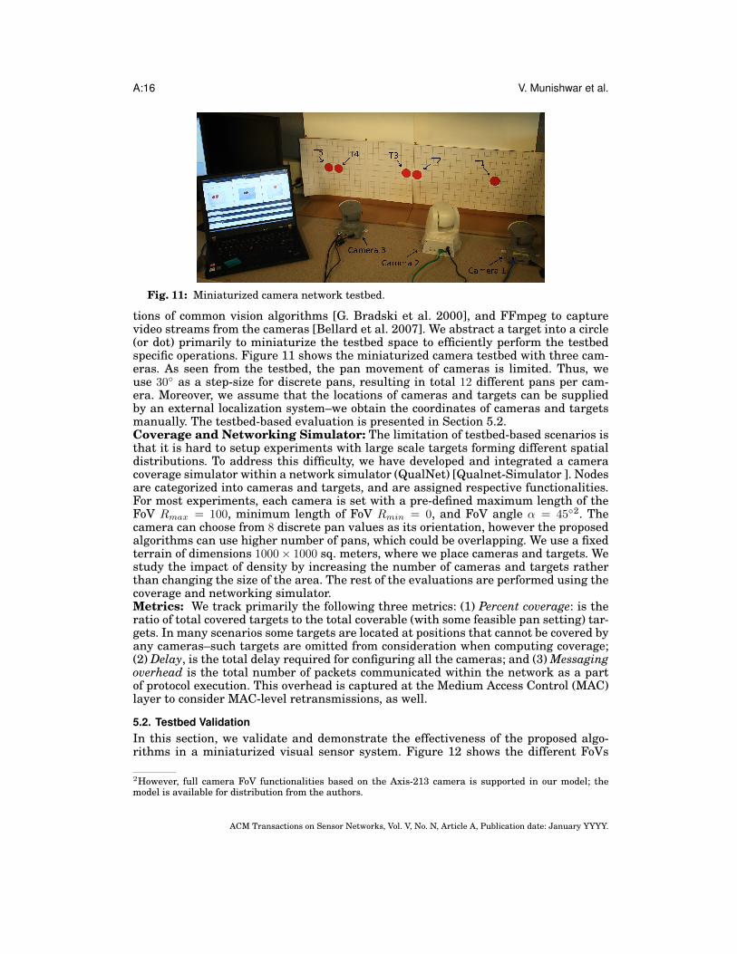
Fig. 11: Miniaturized camera network testbed.
tions of common vision algorithms [G. Bradski et al. 2000], and FFmpeg to capturevideo streams from the cameras [Bellard et al. 2007]. We abstract a target into a circle(or dot) primarily to miniaturize the testbed space to efficiently perform the testbedspecific operations. Figure 11 shows the miniaturized camera testbed with three cam-eras. As seen from the testbed, the pan movement of cameras is limited. Thus, weuse 30◦ as a step-size for discrete pans, resulting in total 12 different pans per cam-era. Moreover, we assume that the locations of cameras and targets can be suppliedby an external localization system–we obtain the coordinates of cameras and targetsmanually. The testbed-based evaluation is presented in Section 5.2.Coverage and Networking Simulator: The limitation of testbed-based scenarios isthat it is hard to setup experiments with large scale targets forming different spatialdistributions. To address this difficulty, we have developed and integrated a cameracoverage simulator within a network simulator (QualNet) [Qualnet-Simulator ]. Nodesare categorized into cameras and targets, and are assigned respective functionalities.For most experiments, each camera is set with a pre-defined maximum length of theFoV Rmax = 100, minimum length of FoV Rmin = 0, and FoV angle α = 45◦2. Thecamera can choose from 8 discrete pan values as its orientation, however the proposedalgorithms can use higher number of pans, which could be overlapping. We use a fixedterrain of dimensions 1000× 1000 sq. meters, where we place cameras and targets. Westudy the impact of density by increasing the number of cameras and targets ratherthan changing the size of the area. The rest of the evaluations are performed using thecoverage and networking simulator.Metrics: We track primarily the following three metrics: (1) Percent coverage: is theratio of total covered targets to the total coverable (with some feasible pan setting) tar-gets. In many scenarios some targets are located at positions that cannot be covered byany cameras–such targets are omitted from consideration when computing coverage;(2) Delay, is the total delay required for configuring all the cameras; and (3) Messagingoverhead is the total number of packets communicated within the network as a partof protocol execution. This overhead is captured at the Medium Access Control (MAC)layer to consider MAC-level retransmissions, as well.
5.2. Testbed ValidationIn this section, we validate and demonstrate the effectiveness of the proposed algo-rithms in a miniaturized visual sensor system. Figure 12 shows the different FoVs
2However, full camera FoV functionalities based on the Axis-213 camera is supported in our model; themodel is available for distribution from the authors.
ACM Transactions on Sensor Networks, Vol. V, No. N, Article A, Publication date: January YYYY.
Coverage Algorithms for Visual Sensor Networks A:17
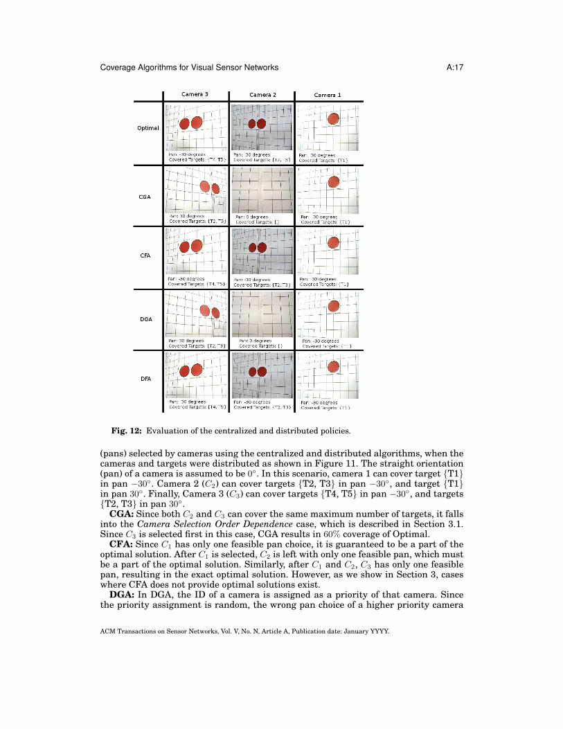
Fig. 12: Evaluation of the centralized and distributed policies.
(pans) selected by cameras using the centralized and distributed algorithms, when thecameras and targets were distributed as shown in Figure 11. The straight orientation(pan) of a camera is assumed to be 0◦. In this scenario, camera 1 can cover target {T1}in pan −30◦. Camera 2 (C2) can cover targets {T2, T3} in pan −30◦, and target {T1}in pan 30◦. Finally, Camera 3 (C3) can cover targets {T4, T5} in pan −30◦, and targets{T2, T3} in pan 30◦.
CGA: Since both C2 and C3 can cover the same maximum number of targets, it fallsinto the Camera Selection Order Dependence case, which is described in Section 3.1.Since C3 is selected first in this case, CGA results in 60% coverage of Optimal.
CFA: Since C1 has only one feasible pan choice, it is guaranteed to be a part of theoptimal solution. After C1 is selected, C2 is left with only one feasible pan, which mustbe a part of the optimal solution. Similarly, after C1 and C2, C3 has only one feasiblepan, resulting in the exact optimal solution. However, as we show in Section 3, caseswhere CFA does not provide optimal solutions exist.
DGA: In DGA, the ID of a camera is assigned as a priority of that camera. Sincethe priority assignment is random, the wrong pan choice of a higher priority camera
ACM Transactions on Sensor Networks, Vol. V, No. N, Article A, Publication date: January YYYY.
A:18 V. Munishwar et al.
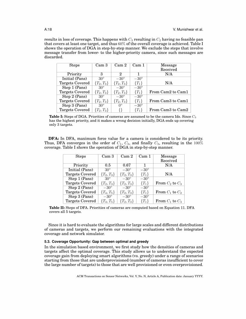
results in loss of coverage. This happens with C3 resulting in C2 having no feasible panthat covers at least one target, and thus 60% of the overall coverage is achieved. Table Ishows the operation of DGA in step-by-step manner. We exclude the steps that involvemessage transfer from lower- to the higher-priority camera, since such messages arediscarded.
Steps Cam 3 Cam 2 Cam 1 MessageReceived
Priority 3 2 1 N/AInitial (Pans) 30◦ −30◦ −30◦
Targets Covered {T2, T3} {T2, T3} {T1} N/AStep 1 (Pans) 30◦ −30◦ −30◦
Targets Covered {T2, T3} {T2, T3} {T1} From Cam2 to Cam1Step 2 (Pans) 30◦ −30◦ −30◦
Targets Covered {T2, T3} {T2, T3} {T1} From Cam3 to Cam1Step 3 (Pans) 30◦ 0◦ −30◦
Targets Covered {T2, T3} {} {T1} From Cam3 to Cam2
Table I: Steps of DGA. Priorities of cameras are assumed to be the camera Ids. Since C3
has the highest priority, and it makes a wrong decision initially, DGA ends up coveringonly 3 targets.
DFA: In DFA, maximum force value for a camera is considered to be its priority.Thus, DFA converges in the order of C1, C2, and finally C3, resulting in the 100%coverage. Table I shows the operation of DGA in step-by-step manner.
Steps Cam 3 Cam 2 Cam 1 MessageReceived
Priority 0.5 0.67 1 N/AInitial (Pans) 30◦ −30◦ −30◦
Targets Covered {T2, T3} {T2, T3} {T1} N/AStep 1 (Pans) 30◦ −30◦ −30◦
Targets Covered {T2, T3} {T2, T3} {T1} From C2 to C3
Step 2 (Pans) −30◦ −30◦ −30◦Targets Covered {T4, T5} {T2, T3} {T1} From C1 to C2
Step 3 (Pans) −30◦ −30◦ −30◦Targets Covered {T4, T5} {T2, T3} {T1} From C1 to C3
Table II: Steps of DFA. Priorities of cameras are computed based on Equation 11. DFAcovers all 5 targets.
Since it is hard to evaluate the algorithms for large scales and different distributionsof cameras and targets, we perform our remaining evaluations with the integratedcoverage and network simulator.
5.3. Coverage Opportunity: Gap between optimal and greedyIn the simulation based environment, we first study how the densities of cameras andtargets affect the optimal coverage. This study allows us to understand the expectedcoverage gain from deploying smart algorithms (vs. greedy) under a range of scenariosstarting from those that are underprovisioned (number of cameras insufficient to coverthe large number of targets) to those that are well provisioned or even overprovisioned.
ACM Transactions on Sensor Networks, Vol. V, No. N, Article A, Publication date: January YYYY.
Coverage Algorithms for Visual Sensor Networks A:19
2030
4050
6070
8090
100
20
40
60
80
10040
50
60
70
80
90
100
CamerasTargets
Pe
rce
nt
Co
ve
rag
e
Fig. 13: Impact on total targets covered20
40
60
80
100
20
40
60
80
100
4
6
8
10
12
14
16
18
20
CamerasTargets
Pe
rce
nt
Co
ve
rag
e:
Op
tim
al−
Gre
ed
y
6
8
10
12
14
16
18
Fig. 14: Gap between Optimal and Greedy
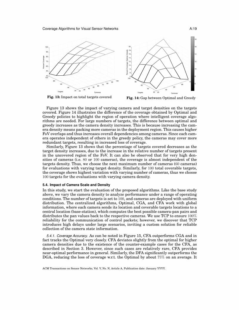
Figure 13 shows the impact of varying camera and target densities on the targetscovered. Figure 14 illustrates the difference of the coverage obtained by Optimal andGreedy policies to highlight the region of operation where intelligent coverage algo-rithms are needed. For large numbers of targets, the difference between optimal andgreedy increases as the camera density increases. This is because increasing the cam-era density means packing more cameras in the deployment region. This causes higherFoV overlaps and thus increases overall dependencies among cameras. Since each cam-era operates independent of others in the greedy policy, the cameras may cover moreredundant targets, resulting in increased loss of coverage.
Similarly, Figure 13 shows that the percentage of targets covered decreases as thetarget density increases, due to the increase in the relative number of targets presentin the uncovered region of the FoV. It can also be observed that for very high den-sities of cameras (i.e. 80 or 100 cameras), the coverage is almost independent of thetargets density. Thus, we choose the next maximum number of cameras (60 cameras)for evaluations with varying target density. Similarly, for 100 total coverable targets,the coverage shows highest variation with varying number of cameras, thus we choose100 targets for the evaluations with varying camera density.
5.4. Impact of Camera Scale and DensityIn this study, we start the evaluation of the proposed algorithms. Like the base studyabove, we vary the camera density to analyze performance under a range of operatingconditions. The number of targets is set to 100, and cameras are deployed with uniformdistribution. The centralized algorithms, Optimal, CGA, and CFA work with globalinformation, where each camera sends its location and coverable targets locations to acentral location (base-station), which computes the best possible camera-pan pairs anddistributes the pan values back to the respective cameras. We use TCP to ensure 100%reliability for the communication of control packets; however, we discover that TCPintroduces high delays under large scenarios, inviting a custom solution for reliablecollection of the camera state information.
5.4.1. Coverage Accuracy. As can be noted in Figure 15, CFA outperforms CGA and infact tracks the Optimal very closely. CFA deviates slightly from the optimal for highercamera densities due to the existence of the counter-example cases for the CFA, asdescribed in Section 3. However, since such cases are relatively rare, CFA providesnear-optimal performance in general. Similarly, the DFA significantly outperforms theDGA, reducing the loss of coverage w.r.t. the Optimal by about 75% on an average. It
ACM Transactions on Sensor Networks, Vol. V, No. N, Article A, Publication date: January YYYY.
A:20 V. Munishwar et al.
20 30 40 50 60 70 80 90 100
40
50
60
70
80
90
100
Cameras
Pe
rce
nt
Co
ve
rag
e
Optimal
CGA
CFA
DGA
DFA
Greedy
Fig. 15: Impact of camera density oncoverage.
20 30 40 50 60 70 80 90 100
0
200
400
600
800
1000
1200
1400
1600
1800
2000
Cameras
Nu
mb
er
of Pa
ck
ets
Optimal
CGA
CFA
DGA
DFA
Fig. 16: Impact of camera density onmessaging overhead.
20 30 40 50 60 70 80 90 100
10−1
100
101
102
Cameras
Av
g.
E2
E D
ela
y (
sec
on
ds)
Optimal
CGA
CFA
DGA
DFA
Fig. 17: Impact of camera density onend-to-end delay.
0200
400600
8001000
0
500
10000
5
10
15
20
25
30
XY
De
lay
Fig. 18: End-to-end delay (in seconds)per camera for centralized policies.
is more interesting to note that the proposed distributed algorithm, DFA, even outper-forms the existing centralized algorithm, CGA.
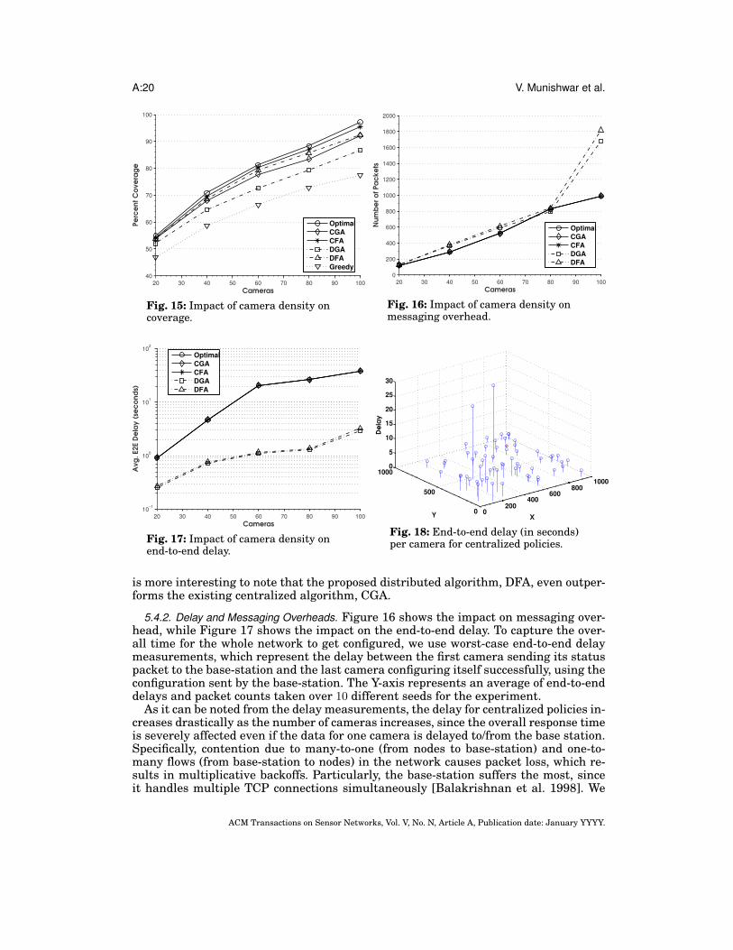
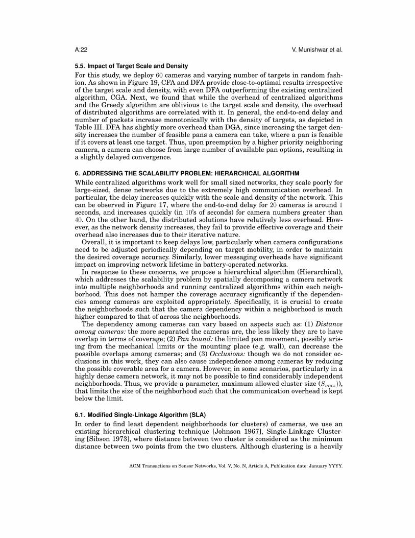
5.4.2. Delay and Messaging Overheads. Figure 16 shows the impact on messaging over-head, while Figure 17 shows the impact on the end-to-end delay. To capture the over-all time for the whole network to get configured, we use worst-case end-to-end delaymeasurements, which represent the delay between the first camera sending its statuspacket to the base-station and the last camera configuring itself successfully, using theconfiguration sent by the base-station. The Y-axis represents an average of end-to-enddelays and packet counts taken over 10 different seeds for the experiment.
As it can be noted from the delay measurements, the delay for centralized policies in-creases drastically as the number of cameras increases, since the overall response timeis severely affected even if the data for one camera is delayed to/from the base station.Specifically, contention due to many-to-one (from nodes to base-station) and one-to-many flows (from base-station to nodes) in the network causes packet loss, which re-sults in multiplicative backoffs. Particularly, the base-station suffers the most, sinceit handles multiple TCP connections simultaneously [Balakrishnan et al. 1998]. We
ACM Transactions on Sensor Networks, Vol. V, No. N, Article A, Publication date: January YYYY.
Coverage Algorithms for Visual Sensor Networks A:21
20 30 40 50 60 70 80 90 100
60
65
70
75
80
85
90
95
100
Targets
Pe
rce
nt
Co
ve
rag
e
Optimal
CGA
CFA
DGA
DFA
Greedy
Fig. 19: Impact of varying target density on coverage.
Targets Avg. E2E Delay Number of PacketsDGA DFA DGA DFA
20 0.52 0.53 277.40 282.1040 0.70 0.73 403.80 416.3060 0.82 0.88 488.60 510.1080 0.88 0.93 518.00 544.70
100 0.90 0.95 536.80 562.80
Table III: Avg. end-to-end delay (in seconds) and number of packets for DGA and DFA.Other policies are omitted because their overhead is independent of target density.
also observe destructive interactions with the TCP congestion management algorithmwhere packet losses cause exponential backoff of the retransmit timer adding to theoverall delay.
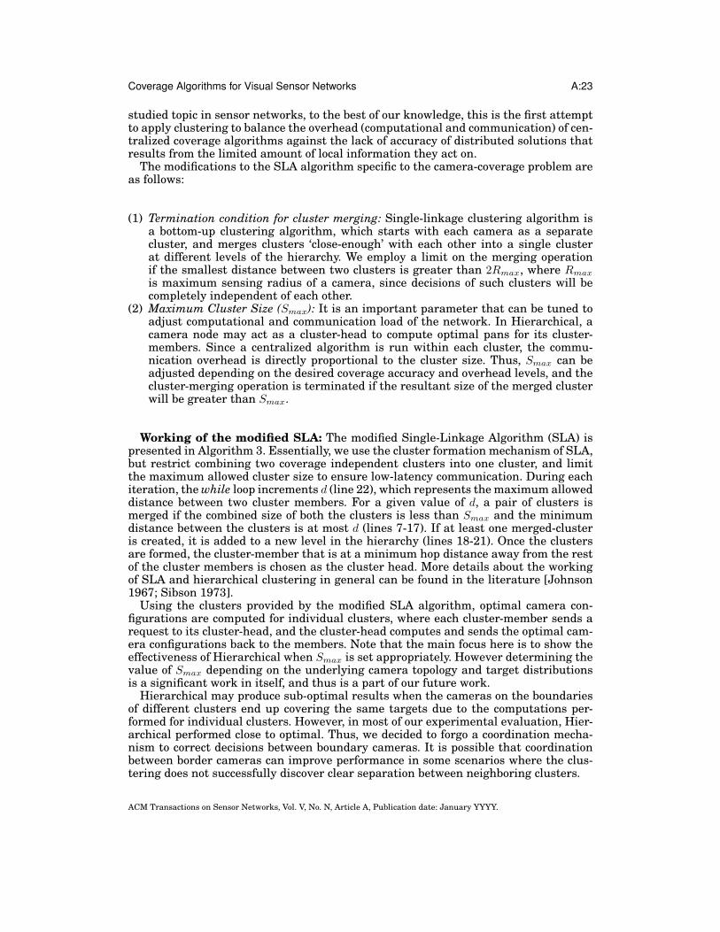
Figure 18 shows per camera end-to-end delay (on Z-axis) for running the Optimalpolicy. The X- and Y-axis represent X and Y coordinates of cameras on the terrain, re-spectively, and the small circles represent cameras deployed on the terrain. The shadedcircle shows the location of the base-station (randomly placed) for this scenario. As itcan be noted, the delays for only two cameras are order of magnitude higher thanthe remaining cameras. Since there is no traffic other than the control packets, thesedelays are the artifacts of TCP’s congestion control mechanism.
The distributed algorithms incur relatively less convergence delay, but even they aresusceptible to delays, as the network scale and density increase. This delay is due totheir inherently iterative nature–they converge from the highest to the lowest prioritycameras, in general.
In terms of messaging overhead, for lower camera density, both the centralized anddistributed algorithms transmit the same number of packets, while for the increasedcamera density, packet overhead increases due to the increased medium access con-tention and packet loss in the network. The high messaging overhead of the distributedalgorithms for high camera density is due to the increase in the number of neighboringcameras for each camera.
ACM Transactions on Sensor Networks, Vol. V, No. N, Article A, Publication date: January YYYY.
A:22 V. Munishwar et al.
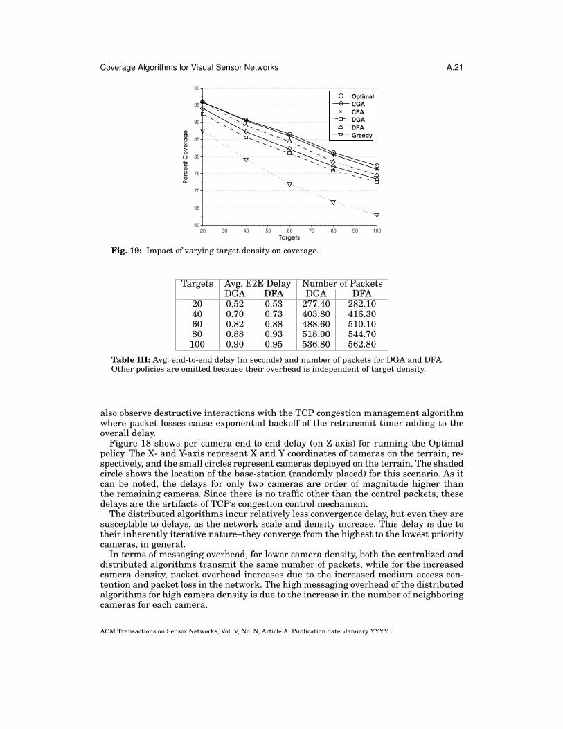
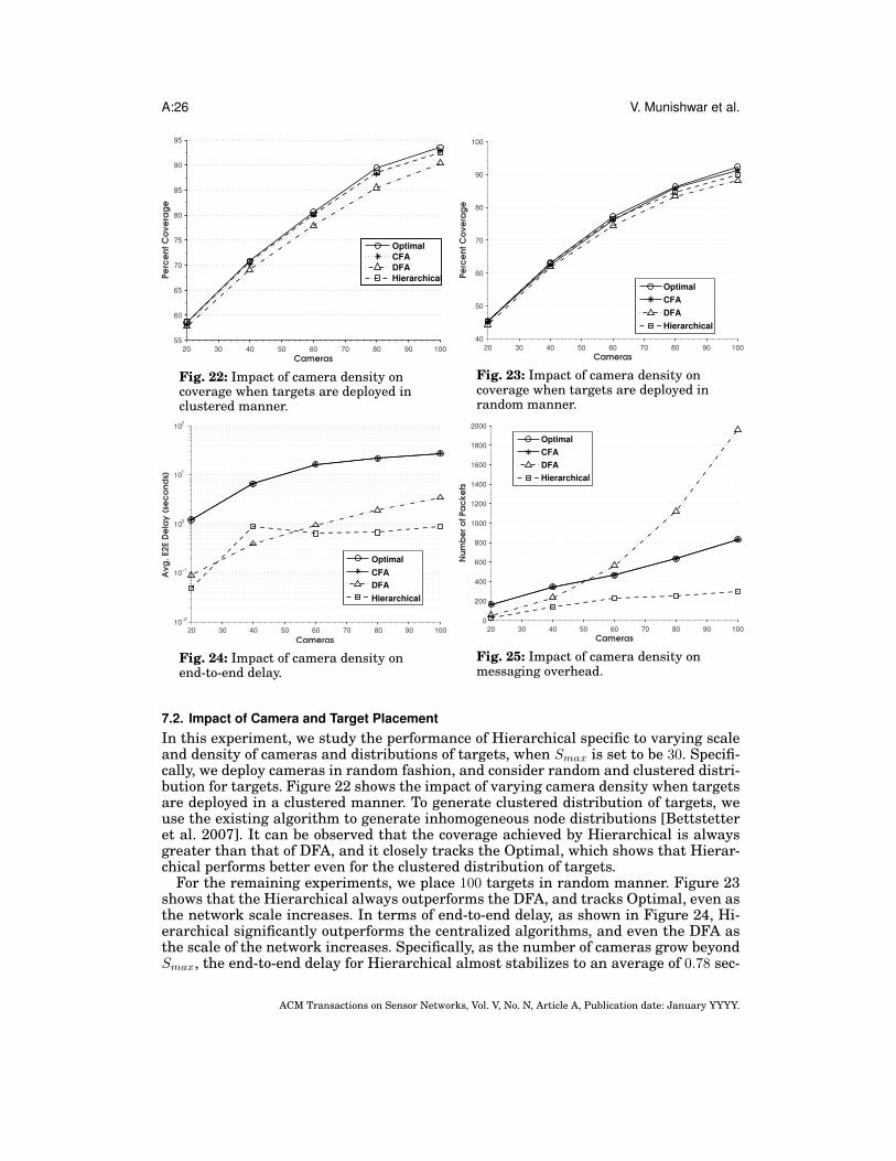
5.5. Impact of Target Scale and DensityFor this study, we deploy 60 cameras and varying number of targets in random fash-ion. As shown in Figure 19, CFA and DFA provide close-to-optimal results irrespectiveof the target scale and density, with even DFA outperforming the existing centralizedalgorithm, CGA. Next, we found that while the overhead of centralized algorithmsand the Greedy algorithm are oblivious to the target scale and density, the overheadof distributed algorithms are correlated with it. In general, the end-to-end delay andnumber of packets increase monotonically with the density of targets, as depicted inTable III. DFA has slightly more overhead than DGA, since increasing the target den-sity increases the number of feasible pans a camera can take, where a pan is feasibleif it covers at least one target. Thus, upon preemption by a higher priority neighboringcamera, a camera can choose from large number of available pan options, resulting ina slightly delayed convergence.
6. ADDRESSING THE SCALABILITY PROBLEM: HIERARCHICAL ALGORITHMWhile centralized algorithms work well for small sized networks, they scale poorly forlarge-sized, dense networks due to the extremely high communication overhead. Inparticular, the delay increases quickly with the scale and density of the network. Thiscan be observed in Figure 17, where the end-to-end delay for 20 cameras is around 1seconds, and increases quickly (in 10’s of seconds) for camera numbers greater than40. On the other hand, the distributed solutions have relatively less overhead. How-ever, as the network density increases, they fail to provide effective coverage and theiroverhead also increases due to their iterative nature.
Overall, it is important to keep delays low, particularly when camera configurationsneed to be adjusted periodically depending on target mobility, in order to maintainthe desired coverage accuracy. Similarly, lower messaging overheads have significantimpact on improving network lifetime in battery-operated networks.
In response to these concerns, we propose a hierarchical algorithm (Hierarchical),which addresses the scalability problem by spatially decomposing a camera networkinto multiple neighborhoods and running centralized algorithms within each neigh-borhood. This does not hamper the coverage accuracy significantly if the dependen-cies among cameras are exploited appropriately. Specifically, it is crucial to createthe neighborhoods such that the camera dependency within a neighborhood is muchhigher compared to that of across the neighborhoods.
The dependency among cameras can vary based on aspects such as: (1) Distanceamong cameras: the more separated the cameras are, the less likely they are to haveoverlap in terms of coverage; (2) Pan bound: the limited pan movement, possibly aris-ing from the mechanical limits or the mounting place (e.g. wall), can decrease thepossible overlaps among cameras; and (3) Occlusions: though we do not consider oc-clusions in this work, they can also cause independence among cameras by reducingthe possible coverable area for a camera. However, in some scenarios, particularly in ahighly dense camera network, it may not be possible to find considerably independentneighborhoods. Thus, we provide a parameter, maximum allowed cluster size (Smax)),that limits the size of the neighborhood such that the communication overhead is keptbelow the limit.
6.1. Modified Single-Linkage Algorithm (SLA)In order to find least dependent neighborhoods (or clusters) of cameras, we use anexisting hierarchical clustering technique [Johnson 1967], Single-Linkage Cluster-ing [Sibson 1973], where distance between two cluster is considered as the minimumdistance between two points from the two clusters. Although clustering is a heavily
ACM Transactions on Sensor Networks, Vol. V, No. N, Article A, Publication date: January YYYY.
Coverage Algorithms for Visual Sensor Networks A:23
studied topic in sensor networks, to the best of our knowledge, this is the first attemptto apply clustering to balance the overhead (computational and communication) of cen-tralized coverage algorithms against the lack of accuracy of distributed solutions thatresults from the limited amount of local information they act on.
The modifications to the SLA algorithm specific to the camera-coverage problem areas follows:
(1) Termination condition for cluster merging: Single-linkage clustering algorithm isa bottom-up clustering algorithm, which starts with each camera as a separatecluster, and merges clusters ‘close-enough’ with each other into a single clusterat different levels of the hierarchy. We employ a limit on the merging operationif the smallest distance between two clusters is greater than 2Rmax, where Rmax
is maximum sensing radius of a camera, since decisions of such clusters will becompletely independent of each other.
(2) Maximum Cluster Size (Smax): It is an important parameter that can be tuned toadjust computational and communication load of the network. In Hierarchical, acamera node may act as a cluster-head to compute optimal pans for its cluster-members. Since a centralized algorithm is run within each cluster, the commu-nication overhead is directly proportional to the cluster size. Thus, Smax can beadjusted depending on the desired coverage accuracy and overhead levels, and thecluster-merging operation is terminated if the resultant size of the merged clusterwill be greater than Smax.
Working of the modified SLA: The modified Single-Linkage Algorithm (SLA) ispresented in Algorithm 3. Essentially, we use the cluster formation mechanism of SLA,but restrict combining two coverage independent clusters into one cluster, and limitthe maximum allowed cluster size to ensure low-latency communication. During eachiteration, the while loop increments d (line 22), which represents the maximum alloweddistance between two cluster members. For a given value of d, a pair of clusters ismerged if the combined size of both the clusters is less than Smax and the minimumdistance between the clusters is at most d (lines 7-17). If at least one merged-clusteris created, it is added to a new level in the hierarchy (lines 18-21). Once the clustersare formed, the cluster-member that is at a minimum hop distance away from the restof the cluster members is chosen as the cluster head. More details about the workingof SLA and hierarchical clustering in general can be found in the literature [Johnson1967; Sibson 1973].
Using the clusters provided by the modified SLA algorithm, optimal camera con-figurations are computed for individual clusters, where each cluster-member sends arequest to its cluster-head, and the cluster-head computes and sends the optimal cam-era configurations back to the members. Note that the main focus here is to show theeffectiveness of Hierarchical when Smax is set appropriately. However determining thevalue of Smax depending on the underlying camera topology and target distributionsis a significant work in itself, and thus is a part of our future work.
Hierarchical may produce sub-optimal results when the cameras on the boundariesof different clusters end up covering the same targets due to the computations per-formed for individual clusters. However, in most of our experimental evaluation, Hier-archical performed close to optimal. Thus, we decided to forgo a coordination mecha-nism to correct decisions between boundary cameras. It is possible that coordinationbetween border cameras can improve performance in some scenarios where the clus-tering does not successfully discover clear separation between neighboring clusters.
ACM Transactions on Sensor Networks, Vol. V, No. N, Article A, Publication date: January YYYY.
A:24 V. Munishwar et al.
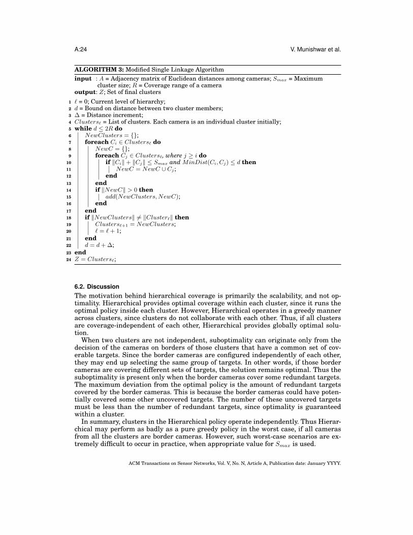
ALGORITHM 3: Modified Single Linkage Algorithminput : A = Adjacency matrix of Euclidean distances among cameras; Smax = Maximum
cluster size; R = Coverage range of a cameraoutput: Z; Set of final clusters
1 ` = 0; Current level of hierarchy;2 d = Bound on distance between two cluster members;3 ∆ = Distance increment;4 Clusters` = List of clusters. Each camera is an individual cluster initially;5 while d ≤ 2R do6 NewClusters = {};7 foreach Ci ∈ Clusters` do8 NewC = {};9 foreach Cj ∈ Clusters`, where j ≥ i do
10 if ‖Ci‖+ ‖Cj‖ ≤ Smax and MinDist(Ci, Cj) ≤ d then11 NewC = NewC ∪ Cj ;12 end13 end14 if ‖NewC‖ > 0 then15 add(NewClusters,NewC);16 end17 end18 if ‖NewClusters‖ 6= ‖Cluster`‖ then19 Clusters`+1 = NewClusters;20 ` = ` + 1;21 end22 d = d + ∆;23 end24 Z = Clusters`;
6.2. DiscussionThe motivation behind hierarchical coverage is primarily the scalability, and not op-timality. Hierarchical provides optimal coverage within each cluster, since it runs theoptimal policy inside each cluster. However, Hierarchical operates in a greedy manneracross clusters, since clusters do not collaborate with each other. Thus, if all clustersare coverage-independent of each other, Hierarchical provides globally optimal solu-tion.
When two clusters are not independent, suboptimality can originate only from thedecision of the cameras on borders of those clusters that have a common set of cov-erable targets. Since the border cameras are configured independently of each other,they may end up selecting the same group of targets. In other words, if those bordercameras are covering different sets of targets, the solution remains optimal. Thus thesuboptimality is present only when the border cameras cover some redundant targets.The maximum deviation from the optimal policy is the amount of redundant targetscovered by the border cameras. This is because the border cameras could have poten-tially covered some other uncovered targets. The number of these uncovered targetsmust be less than the number of redundant targets, since optimality is guaranteedwithin a cluster.
In summary, clusters in the Hierarchical policy operate independently. Thus Hierar-chical may perform as badly as a pure greedy policy in the worst case, if all camerasfrom all the clusters are border cameras. However, such worst-case scenarios are ex-tremely difficult to occur in practice, when appropriate value for Smax is used.
ACM Transactions on Sensor Networks, Vol. V, No. N, Article A, Publication date: January YYYY.
Coverage Algorithms for Visual Sensor Networks A:25
10 15 20 25 30 35 40 45 50 55 60
74.5
75
75.5
76
76.5
77
77.5
Max. Cluster Size
Pe
rce
nt
Co
ve
rag
e
Optimal
CFA
DFA
Hierarchical
Fig. 20: Impact of Smax on coverage
10 15 20 25 30 35 40 45 50 55 60
10−1
100
101
102
Max. Cluster Size
Av
g.
E2
E D
ela
y (
sec
on
ds)
Optimal
CFA
DFA
Hierarchical
Fig. 21: Impact of Smax on end-to-enddelay (Optimal and CFA areoverlapping.)
7. EVALUATION: HIERARCHICAL ALGORITHMIn this section, we present evaluation of the hierarchical algorithm with respect tothe proposed centralized (Optimal, CFA) and distributed (DFA) algorithms for varyingcamera and target density. We do not consider the other policies since the force-directedalgorithms provide better coverage with equal overheads. The goal of this section is toevaluate (1) tunability of Smax and its impact on coverage; and (2) impact of spatialdecomposition of the network on communication overheads. We first study the impactof Smax on coverage and overhead in order to determine an appropriate value for theparameter. We then use this value of Smax for the remaining experiments and presentour evaluations.
7.1. Determining Smax
Based on the study presented in Section 5.3, we set the number of cameras to be 60, andthe number of targets to be 100, and track coverage accuracy and end-to-end delay fordifferent values of Smax. Cameras and targets are deployed in random manner. For thehierarchical algorithm, end-to-end delay is computed for each cluster, and maximumdelay is considered as worst-case delay.
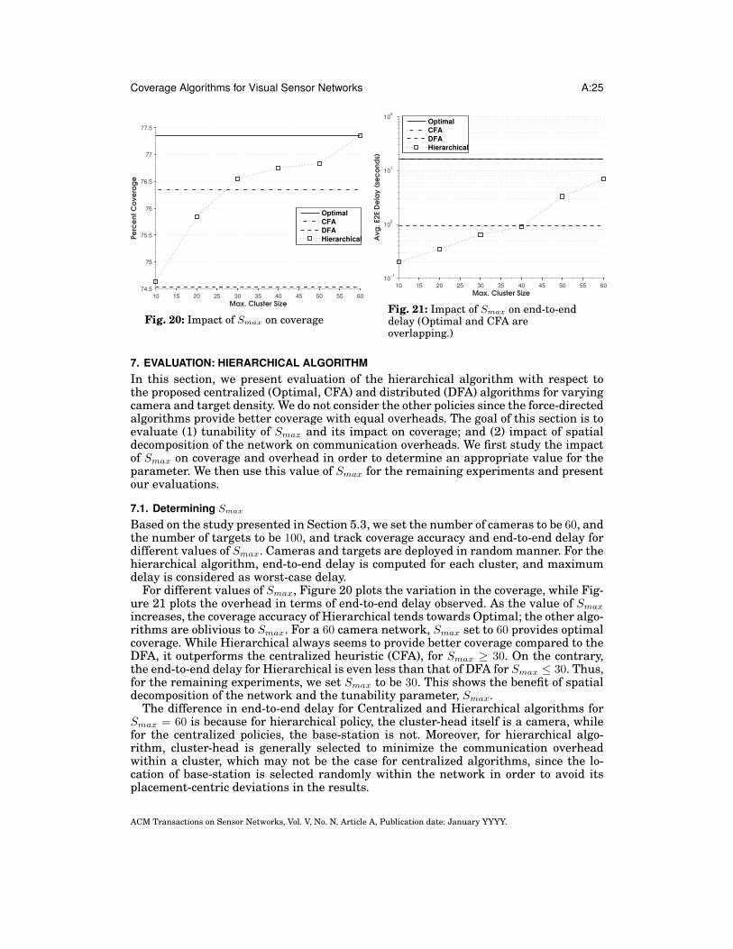
For different values of Smax, Figure 20 plots the variation in the coverage, while Fig-ure 21 plots the overhead in terms of end-to-end delay observed. As the value of Smax
increases, the coverage accuracy of Hierarchical tends towards Optimal; the other algo-rithms are oblivious to Smax. For a 60 camera network, Smax set to 60 provides optimalcoverage. While Hierarchical always seems to provide better coverage compared to theDFA, it outperforms the centralized heuristic (CFA), for Smax ≥ 30. On the contrary,the end-to-end delay for Hierarchical is even less than that of DFA for Smax ≤ 30. Thus,for the remaining experiments, we set Smax to be 30. This shows the benefit of spatialdecomposition of the network and the tunability parameter, Smax.
The difference in end-to-end delay for Centralized and Hierarchical algorithms forSmax = 60 is because for hierarchical policy, the cluster-head itself is a camera, whilefor the centralized policies, the base-station is not. Moreover, for hierarchical algo-rithm, cluster-head is generally selected to minimize the communication overheadwithin a cluster, which may not be the case for centralized algorithms, since the lo-cation of base-station is selected randomly within the network in order to avoid itsplacement-centric deviations in the results.
ACM Transactions on Sensor Networks, Vol. V, No. N, Article A, Publication date: January YYYY.
A:26 V. Munishwar et al.
20 30 40 50 60 70 80 90 100
55
60
65
70
75
80
85
90
95
Cameras
Pe
rce
nt
Co
ve
rag
e
Optimal
CFA
DFA
Hierarchical
Fig. 22: Impact of camera density oncoverage when targets are deployed inclustered manner.
20 30 40 50 60 70 80 90 100
40
50
60
70
80
90
100
Cameras
Pe
rce
nt
Co
ve
rag
e
Optimal
CFA
DFA
Hierarchical
Fig. 23: Impact of camera density oncoverage when targets are deployed inrandom manner.
20 30 40 50 60 70 80 90 100
10−2
10−1
100
101
102
Cameras
Av
g.
E2
E D
ela
y (
sec
on
ds)
Optimal
CFA
DFA
Hierarchical
Fig. 24: Impact of camera density onend-to-end delay.
20 30 40 50 60 70 80 90 100
0
200
400
600
800
1000
1200
1400
1600
1800
2000
Cameras
Nu
mb
er
of Pa
ck
ets
Optimal
CFA
DFA
Hierarchical
Fig. 25: Impact of camera density onmessaging overhead.
7.2. Impact of Camera and Target PlacementIn this experiment, we study the performance of Hierarchical specific to varying scaleand density of cameras and distributions of targets, when Smax is set to be 30. Specifi-cally, we deploy cameras in random fashion, and consider random and clustered distri-bution for targets. Figure 22 shows the impact of varying camera density when targetsare deployed in a clustered manner. To generate clustered distribution of targets, weuse the existing algorithm to generate inhomogeneous node distributions [Bettstetteret al. 2007]. It can be observed that the coverage achieved by Hierarchical is alwaysgreater than that of DFA, and it closely tracks the Optimal, which shows that Hierar-chical performs better even for the clustered distribution of targets.
For the remaining experiments, we place 100 targets in random manner. Figure 23shows that the Hierarchical always outperforms the DFA, and tracks Optimal, even asthe network scale increases. In terms of end-to-end delay, as shown in Figure 24, Hi-erarchical significantly outperforms the centralized algorithms, and even the DFA asthe scale of the network increases. Specifically, as the number of cameras grow beyondSmax, the end-to-end delay for Hierarchical almost stabilizes to an average of 0.78 sec-
ACM Transactions on Sensor Networks, Vol. V, No. N, Article A, Publication date: January YYYY.
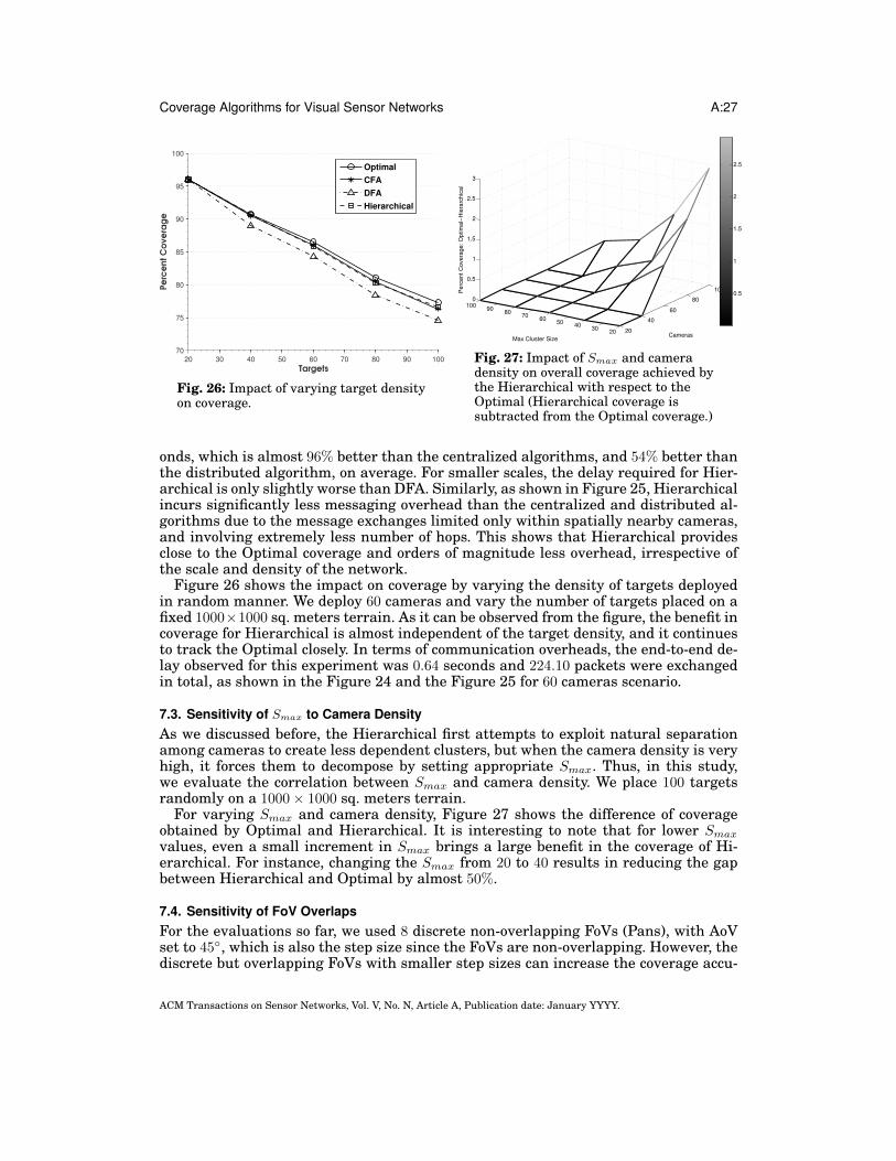
Coverage Algorithms for Visual Sensor Networks A:27
20 30 40 50 60 70 80 90 100
70
75
80
85
90
95
100
Targets
Pe
rce
nt
Co
ve
rag
e
Optimal
CFA
DFA
Hierarchical
Fig. 26: Impact of varying target densityon coverage.
20
40
60
80
100
2030
4050
6070
8090
1000
0.5
1
1.5
2
2.5
3
CamerasMax Cluster Size
Perc
ent C
overa
ge: O
ptim
al−
Hie
rarc
hic
al
0.5
1
1.5
2
2.5
Fig. 27: Impact of Smax and cameradensity on overall coverage achieved bythe Hierarchical with respect to theOptimal (Hierarchical coverage issubtracted from the Optimal coverage.)
onds, which is almost 96% better than the centralized algorithms, and 54% better thanthe distributed algorithm, on average. For smaller scales, the delay required for Hier-archical is only slightly worse than DFA. Similarly, as shown in Figure 25, Hierarchicalincurs significantly less messaging overhead than the centralized and distributed al-gorithms due to the message exchanges limited only within spatially nearby cameras,and involving extremely less number of hops. This shows that Hierarchical providesclose to the Optimal coverage and orders of magnitude less overhead, irrespective ofthe scale and density of the network.
Figure 26 shows the impact on coverage by varying the density of targets deployedin random manner. We deploy 60 cameras and vary the number of targets placed on afixed 1000×1000 sq. meters terrain. As it can be observed from the figure, the benefit incoverage for Hierarchical is almost independent of the target density, and it continuesto track the Optimal closely. In terms of communication overheads, the end-to-end de-lay observed for this experiment was 0.64 seconds and 224.10 packets were exchangedin total, as shown in the Figure 24 and the Figure 25 for 60 cameras scenario.
7.3. Sensitivity of Smax to Camera DensityAs we discussed before, the Hierarchical first attempts to exploit natural separationamong cameras to create less dependent clusters, but when the camera density is veryhigh, it forces them to decompose by setting appropriate Smax. Thus, in this study,we evaluate the correlation between Smax and camera density. We place 100 targetsrandomly on a 1000× 1000 sq. meters terrain.
For varying Smax and camera density, Figure 27 shows the difference of coverageobtained by Optimal and Hierarchical. It is interesting to note that for lower Smax
values, even a small increment in Smax brings a large benefit in the coverage of Hi-erarchical. For instance, changing the Smax from 20 to 40 results in reducing the gapbetween Hierarchical and Optimal by almost 50%.
7.4. Sensitivity of FoV OverlapsFor the evaluations so far, we used 8 discrete non-overlapping FoVs (Pans), with AoVset to 45◦, which is also the step size since the FoVs are non-overlapping. However, thediscrete but overlapping FoVs with smaller step sizes can increase the coverage accu-
ACM Transactions on Sensor Networks, Vol. V, No. N, Article A, Publication date: January YYYY.
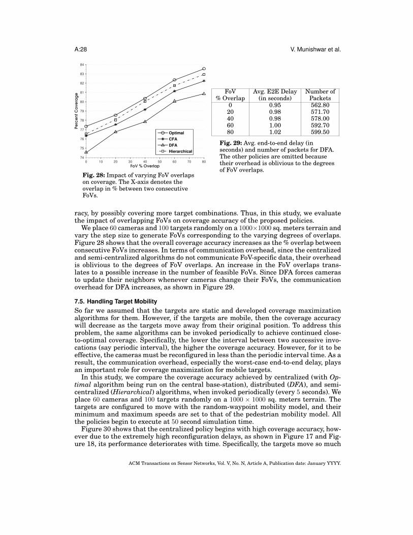
A:28 V. Munishwar et al.
0 10 20 30 40 50 60 70 80
74
75
76
77
78
79
80
81
82
83
84
FoV % Overlap
Pe
rce
nt
Co
ve
rag
e
Optimal
CFA
DFA
Hierarchical
Fig. 28: Impact of varying FoV overlapson coverage. The X-axis denotes theoverlap in % between two consecutiveFoVs.
FoV Avg. E2E Delay Number of% Overlap (in seconds) Packets
0 0.95 562.8020 0.98 571.7040 0.98 578.0060 1.00 592.7080 1.02 599.50
Fig. 29: Avg. end-to-end delay (inseconds) and number of packets for DFA.The other policies are omitted becausetheir overhead is oblivious to the degreesof FoV overlaps.
racy, by possibly covering more target combinations. Thus, in this study, we evaluatethe impact of overlapping FoVs on coverage accuracy of the proposed policies.
We place 60 cameras and 100 targets randomly on a 1000×1000 sq. meters terrain andvary the step size to generate FoVs corresponding to the varying degrees of overlaps.Figure 28 shows that the overall coverage accuracy increases as the % overlap betweenconsecutive FoVs increases. In terms of communication overhead, since the centralizedand semi-centralized algorithms do not communicate FoV-specific data, their overheadis oblivious to the degrees of FoV overlaps. An increase in the FoV overlaps trans-lates to a possible increase in the number of feasible FoVs. Since DFA forces camerasto update their neighbors whenever cameras change their FoVs, the communicationoverhead for DFA increases, as shown in Figure 29.
7.5. Handling Target MobilitySo far we assumed that the targets are static and developed coverage maximizationalgorithms for them. However, if the targets are mobile, then the coverage accuracywill decrease as the targets move away from their original position. To address thisproblem, the same algorithms can be invoked periodically to achieve continued close-to-optimal coverage. Specifically, the lower the interval between two successive invo-cations (say periodic interval), the higher the coverage accuracy. However, for it to beeffective, the cameras must be reconfigured in less than the periodic interval time. As aresult, the communication overhead, especially the worst-case end-to-end delay, playsan important role for coverage maximization for mobile targets.
In this study, we compare the coverage accuracy achieved by centralized (with Op-timal algorithm being run on the central base-station), distributed (DFA), and semi-centralized (Hierarchical) algorithms, when invoked periodically (every 5 seconds). Weplace 60 cameras and 100 targets randomly on a 1000 × 1000 sq. meters terrain. Thetargets are configured to move with the random-waypoint mobility model, and theirminimum and maximum speeds are set to that of the pedestrian mobility model. Allthe policies begin to execute at 50 second simulation time.
Figure 30 shows that the centralized policy begins with high coverage accuracy, how-ever due to the extremely high reconfiguration delays, as shown in Figure 17 and Fig-ure 18, its performance deteriorates with time. Specifically, the targets move so much
ACM Transactions on Sensor Networks, Vol. V, No. N, Article A, Publication date: January YYYY.
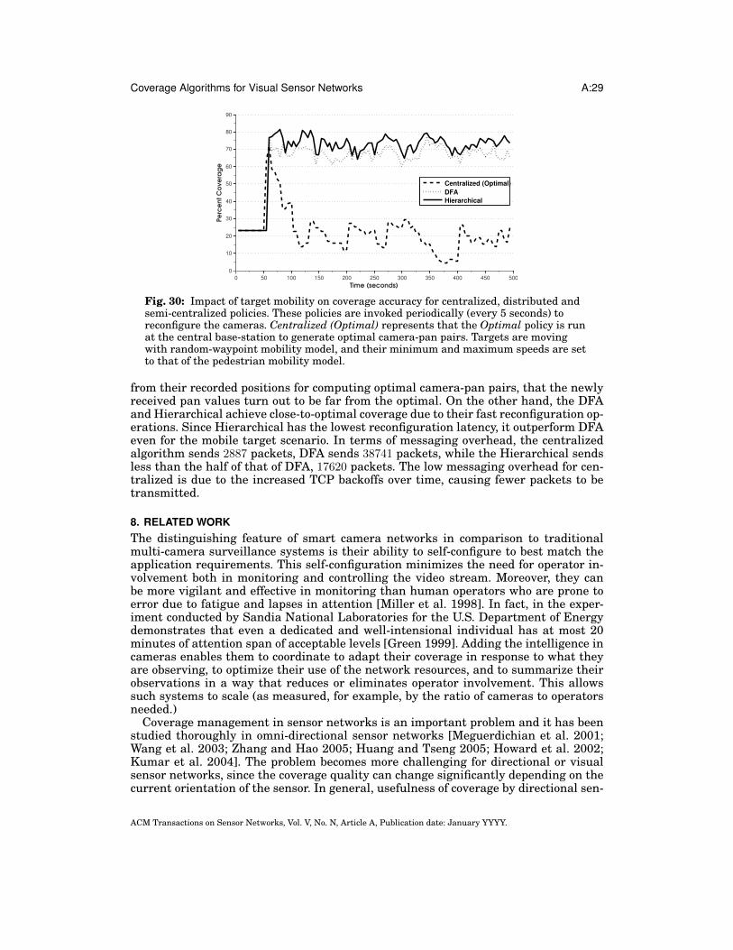
Coverage Algorithms for Visual Sensor Networks A:29
0 50 100 150 200 250 300 350 400 450 500
0
10
20
30
40
50
60
70
80
90
Time (seconds)
Pe
rce
nt
Co
ve
rag
e
Centralized (Optimal)
DFA
Hierarchical
Fig. 30: Impact of target mobility on coverage accuracy for centralized, distributed andsemi-centralized policies. These policies are invoked periodically (every 5 seconds) toreconfigure the cameras. Centralized (Optimal) represents that the Optimal policy is runat the central base-station to generate optimal camera-pan pairs. Targets are movingwith random-waypoint mobility model, and their minimum and maximum speeds are setto that of the pedestrian mobility model.
from their recorded positions for computing optimal camera-pan pairs, that the newlyreceived pan values turn out to be far from the optimal. On the other hand, the DFAand Hierarchical achieve close-to-optimal coverage due to their fast reconfiguration op-erations. Since Hierarchical has the lowest reconfiguration latency, it outperform DFAeven for the mobile target scenario. In terms of messaging overhead, the centralizedalgorithm sends 2887 packets, DFA sends 38741 packets, while the Hierarchical sendsless than the half of that of DFA, 17620 packets. The low messaging overhead for cen-tralized is due to the increased TCP backoffs over time, causing fewer packets to betransmitted.
8. RELATED WORKThe distinguishing feature of smart camera networks in comparison to traditionalmulti-camera surveillance systems is their ability to self-configure to best match theapplication requirements. This self-configuration minimizes the need for operator in-volvement both in monitoring and controlling the video stream. Moreover, they canbe more vigilant and effective in monitoring than human operators who are prone toerror due to fatigue and lapses in attention [Miller et al. 1998]. In fact, in the exper-iment conducted by Sandia National Laboratories for the U.S. Department of Energydemonstrates that even a dedicated and well-intensional individual has at most 20minutes of attention span of acceptable levels [Green 1999]. Adding the intelligence incameras enables them to coordinate to adapt their coverage in response to what theyare observing, to optimize their use of the network resources, and to summarize theirobservations in a way that reduces or eliminates operator involvement. This allowssuch systems to scale (as measured, for example, by the ratio of cameras to operatorsneeded.)
Coverage management in sensor networks is an important problem and it has beenstudied thoroughly in omni-directional sensor networks [Meguerdichian et al. 2001;Wang et al. 2003; Zhang and Hao 2005; Huang and Tseng 2005; Howard et al. 2002;Kumar et al. 2004]. The problem becomes more challenging for directional or visualsensor networks, since the coverage quality can change significantly depending on thecurrent orientation of the sensor. In general, usefulness of coverage by directional sen-
ACM Transactions on Sensor Networks, Vol. V, No. N, Article A, Publication date: January YYYY.
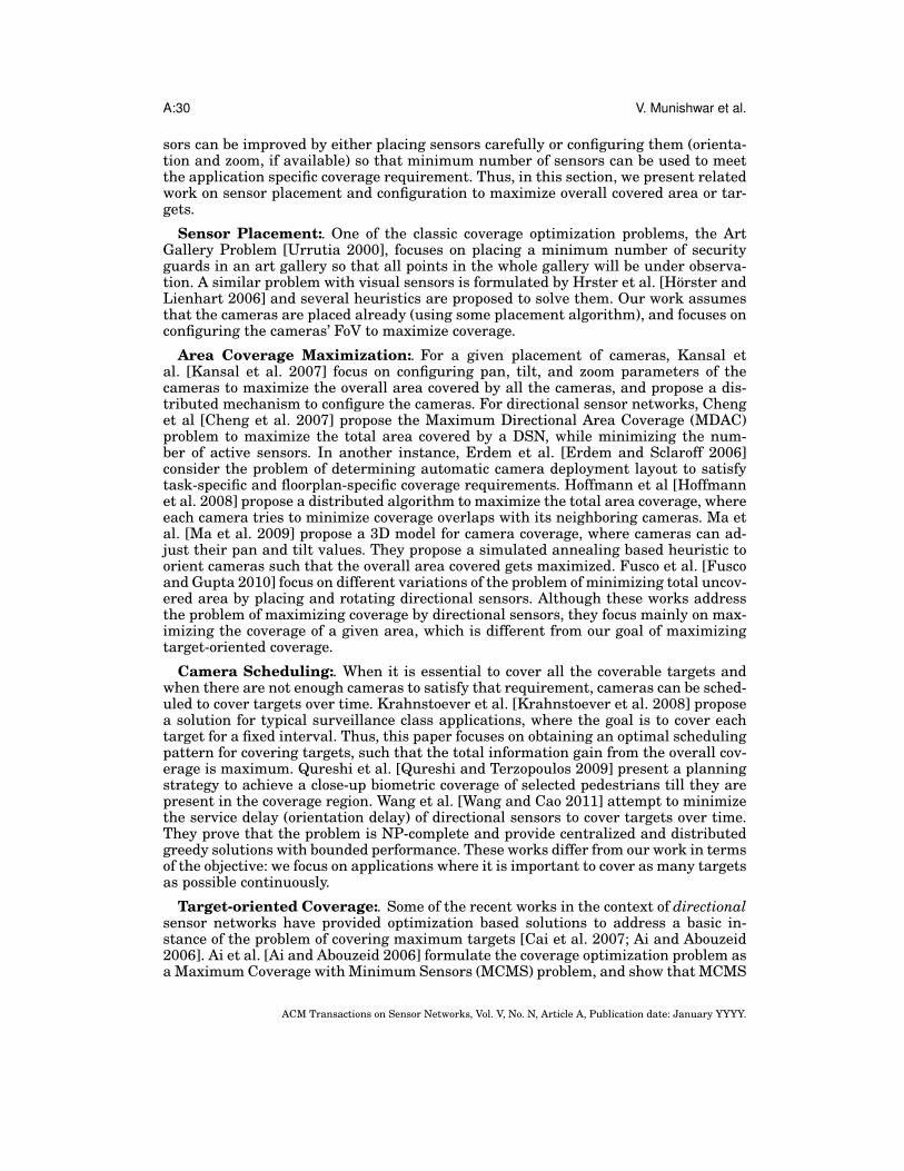
A:30 V. Munishwar et al.
sors can be improved by either placing sensors carefully or configuring them (orienta-tion and zoom, if available) so that minimum number of sensors can be used to meetthe application specific coverage requirement. Thus, in this section, we present relatedwork on sensor placement and configuration to maximize overall covered area or tar-gets.
Sensor Placement:. One of the classic coverage optimization problems, the ArtGallery Problem [Urrutia 2000], focuses on placing a minimum number of securityguards in an art gallery so that all points in the whole gallery will be under observa-tion. A similar problem with visual sensors is formulated by Hrster et al. [Horster andLienhart 2006] and several heuristics are proposed to solve them. Our work assumesthat the cameras are placed already (using some placement algorithm), and focuses onconfiguring the cameras’ FoV to maximize coverage.
Area Coverage Maximization:. For a given placement of cameras, Kansal etal. [Kansal et al. 2007] focus on configuring pan, tilt, and zoom parameters of thecameras to maximize the overall area covered by all the cameras, and propose a dis-tributed mechanism to configure the cameras. For directional sensor networks, Chenget al [Cheng et al. 2007] propose the Maximum Directional Area Coverage (MDAC)problem to maximize the total area covered by a DSN, while minimizing the num-ber of active sensors. In another instance, Erdem et al. [Erdem and Sclaroff 2006]consider the problem of determining automatic camera deployment layout to satisfytask-specific and floorplan-specific coverage requirements. Hoffmann et al [Hoffmannet al. 2008] propose a distributed algorithm to maximize the total area coverage, whereeach camera tries to minimize coverage overlaps with its neighboring cameras. Ma etal. [Ma et al. 2009] propose a 3D model for camera coverage, where cameras can ad-just their pan and tilt values. They propose a simulated annealing based heuristic toorient cameras such that the overall area covered gets maximized. Fusco et al. [Fuscoand Gupta 2010] focus on different variations of the problem of minimizing total uncov-ered area by placing and rotating directional sensors. Although these works addressthe problem of maximizing coverage by directional sensors, they focus mainly on max-imizing the coverage of a given area, which is different from our goal of maximizingtarget-oriented coverage.
Camera Scheduling:. When it is essential to cover all the coverable targets andwhen there are not enough cameras to satisfy that requirement, cameras can be sched-uled to cover targets over time. Krahnstoever et al. [Krahnstoever et al. 2008] proposea solution for typical surveillance class applications, where the goal is to cover eachtarget for a fixed interval. Thus, this paper focuses on obtaining an optimal schedulingpattern for covering targets, such that the total information gain from the overall cov-erage is maximum. Qureshi et al. [Qureshi and Terzopoulos 2009] present a planningstrategy to achieve a close-up biometric coverage of selected pedestrians till they arepresent in the coverage region. Wang et al. [Wang and Cao 2011] attempt to minimizethe service delay (orientation delay) of directional sensors to cover targets over time.They prove that the problem is NP-complete and provide centralized and distributedgreedy solutions with bounded performance. These works differ from our work in termsof the objective: we focus on applications where it is important to cover as many targetsas possible continuously.
Target-oriented Coverage:. Some of the recent works in the context of directionalsensor networks have provided optimization based solutions to address a basic in-stance of the problem of covering maximum targets [Cai et al. 2007; Ai and Abouzeid2006]. Ai et al. [Ai and Abouzeid 2006] formulate the coverage optimization problem asa Maximum Coverage with Minimum Sensors (MCMS) problem, and show that MCMS
ACM Transactions on Sensor Networks, Vol. V, No. N, Article A, Publication date: January YYYY.
Coverage Algorithms for Visual Sensor Networks A:31
is NP-complete. They formulate the MCMS problem as an Integer Linear Program-ming (ILP) problem to propose a centralized algorithm to solve the problem. However,since the centralized algorithm is not scalable, they provide greedy based centralized(CGA) and distributed (DGA) algorithms for coverage maximization for DSNs. Cai etal. [Cai et al. 2007] focus on the problem of maximizing the lifetime of a directionalsensor network. Essentially, they compute Multiple Directional Cover Sets (MDCSs)for a given set of targets. A Directional Cover Set (DCS) is a subset of directions of thesensors, which can cover all the targets present in the area under observation. Thus,by computing multiple such DCSs, they can alternately activate only one DCS at anygiven time, while keeping the other sensors in a sleep state. This helps them increasethe overall network lifetime. The authors show that the problem of computing DCSand MDCS is NP-complete and propose heuristics to solve MDCS. Soto et al. [Sotoet al. 2009] present a game-theoretic algorithm to obtain optimal camera configura-tion to acquire all targets at desired resolution. Fusco et al. [Fusco and Gupta 2009]focus on achieving k-coverage of a given set of targets (or area) using minimum num-ber of directional sensors. They prove the problem to be NP-hard, and propose a greedyalgorithm along with performance guarantees.
In the context of camera networks, Qureshi et al. [Qureshi and Terzopoulos 2008]focus on the problem of selecting cameras to carryout the given tasks, such as trackinga given set of pedestrians. They propose a distributed camera network control strategythat enables performing the surveillance tasks by groups of cameras. For evaluation,they have developed a simulated network of smart cameras that can monitor simu-lated pedestrians in a large virtual public space, such as a train station. In anotherinteresting work, Johnson et al [Johnson and Bar-Noy 2011] focus on configuring panand zoom based cameras (for instance, cameras in unmanned aerial vehicles (UAVs))to cover maximum number of targets with highest precision possible.
Our problem is closely related to that of Ai et al. [Ai and Abouzeid 2006]: and weimplement and use their proposed algorithms as benchmarks for comparison. On theother hand, the works by Cai et al. [Cai et al. 2007] and Soto et al. [Soto et al. 2009] aredifferent since they assume that all the targets can be covered with certain camera-pan configurations. This assumption makes the problem an instance of the set-coverproblem, attempting to find the optimal configuration to minimize the number of sen-sors needed to cover the targets. In contrast, we consider scenarios where the numberof cameras is insufficient to cover the targets, making the problem an instance of themaximum coverage problem [Hochbaum 1996; Ai and Abouzeid 2006].
There is significant research on tracking single or multiple targets [Ercan et al.2007; Porikli and Divakaran 2003; Ukita et al. 2000]. However, this research is notgeared towards maximizing the number of targets under observation (the coveragemaximization problem.)
9. CONCLUSION AND FUTURE WORKIn smart camera networks, coverage control is necessary to allow automatic trackingof targets without human intervention, allowing these systems to scale. In this paper,we consider the problem of automatic control of the cameras to maximize coverage ofa set of targets. We presented an ILP-based formulation of the coverage maximiza-tion problem. Since the ILP problem is NP-hard, we proposed novel centralized (CFA)and distributed (DFA) heuristics that provide near-optimal performance, and providebetter coverage accuracy compared to the state-of-the-art. In fact, even the proposeddistributed algorithm (DFA) outperforms the existing centralized algorithm (CGA).We proved that the centralized and distributed algorithms are 0.5-approximate. Wealso demonstrated the effectiveness of the proposed algorithms using a miniaturizedcamera network testbed.
ACM Transactions on Sensor Networks, Vol. V, No. N, Article A, Publication date: January YYYY.
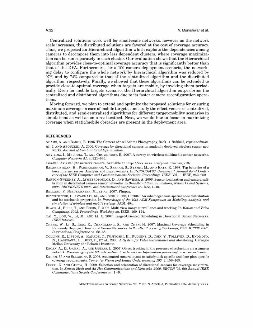
A:32 V. Munishwar et al.
Centralized solutions work well for small-scale networks, however as the networkscale increases, the distributed solutions are favored at the cost of coverage accuracy.Thus, we proposed an Hierarchical algorithm which exploits the dependencies amongcameras to decompose them into less dependent clusters, where coverage maximiza-tion can be run separately in each cluster. Our evaluation shows that the Hierarchicalalgorithm provides close-to-optimal coverage accuracy that is significantly better thanthat of the DFA. Furthermore, for a 100 camera deployment scenario, the network-ing delay to configure the whole network by hierarchical algorithm was reduced by97% and by 74% compared to that of the centralized algorithm and the distributedalgorithm, respectively. Finally, we showed that these algorithms can be extended toprovide close-to-optimal coverage when targets are mobile, by invoking them period-ically. Even for mobile targets scenario, the Hierarchical algorithm outperforms thecentralized and distributed algorithms due to its faster camera reconfiguration opera-tions.
Moving forward, we plan to extend and optimize the proposed solutions for ensuringmaximum coverage in case of mobile targets, and study the effectiveness of centralized,distributed, and semi-centralized algorithms for different target-mobility scenarios insimulations as well as on a real testbed. Next, we would like to focus on maximizingcoverage when static/mobile obstacles are present in the deployment area.
REFERENCESADAMS, A. AND BAKER, R. 1995. The Camera (Ansel Adams Photography, Book 1). Bulfinch, reprint edition.AI, J. AND ABOUZEID, A. 2006. Coverage by directional sensors in randomly deployed wireless sensor net-
works. Journal of Combinatorial Optimization.AKYILDIZ, I., MELODIA, T., AND CHOWDHURY, K. 2007. A survey on wireless multimedia sensor networks.
Computer Networks 51, 4, 921–960.axis-213. Axis 213 ptz network camera. Available at http://www.axis.com/products/cam_213/.BALAKRISHNAN, H., PADMANABHAN, V., SESHAN, S., STEMM, M., AND KATZ, R. 1998. Tcp behavior of a
busy internet server: Analysis and improvements. In INFOCOM’98. Seventeenth Annual Joint Confer-ence of the IEEE Computer and Communications Societies. Proceedings. IEEE. Vol. 1. IEEE, 252–262.
BARTON-SWEENEY, A., LYMBEROPOULOS, D., AND SAWIDES, A. 2006. Sensor localization and camera cali-bration in distributed camera sensor networks. In Broadband Communications, Networks and Systems,2006. BROADNETS 2006. 3rd International Conference on. Ieee, 1–10.
BELLARD, F., NIEDERMAYER, M., ET AL. 2007. Ffmpeg.BETTSTETTER, C., GYARMATI, M., AND SCHILCHER, U. 2007. An inhomogeneous spatial node distribution
and its stochastic properties. In Proceedings of the 10th ACM Symposium on Modeling, analysis, andsimulation of wireless and mobile systems. ACM, 404.
BLACK, J., ELLIS, T., AND ROSIN, P. 2002. Multi view image surveillance and tracking. In Motion and VideoComputing, 2002. Proceedings. Workshop on. IEEE, 169–174.
CAI, Y., LOU, W., LI, M., AND LI, X. 2007. Target-Oriented Scheduling in Directional Sensor Networks.IEEE Infocom.
CHENG, W., LI, S., LIAO, X., CHANGXIANG, S., AND CHEN, H. 2007. Maximal Coverage Scheduling inRandomly Deployed Directional Sensor Networks. In Parallel Processing Workshops, 2007. ICPPW 2007.International Conference on. 68–68.
COLLINS, R., LIPTON, A., KANADE, T., FUJIYOSHI, H., DUGGINS, D., TSIN, Y., TOLLIVER, D., ENOMOTO,N., HASEGAWA, O., BURT, P., ET AL. 2000. A System for Video Surveillance and Monitoring. CarnegieMellon University, the Robotics Institute.
ERCAN, A., EL GAMAL, A., AND GUIBAS, L. 2007. Object tracking in the presence of occlusions via a cameranetwork. Proceedings of the 6th international conference on Information processing in sensor networks.
ERDEM, U. AND SCLAROFF, S. 2006. Automated camera layout to satisfy task-specific and floor plan-specificcoverage requirements. Computer Vision and Image Understanding 103, 3, 156–169.
FUSCO, G. AND GUPTA, H. 2009. Selection and orientation of directional sensors for coverage maximiza-tion. In Sensor, Mesh and Ad Hoc Communications and Networks, 2009. SECON ’09. 6th Annual IEEECommunications Society Conference on. 1 –9.
ACM Transactions on Sensor Networks, Vol. V, No. N, Article A, Publication date: January YYYY.
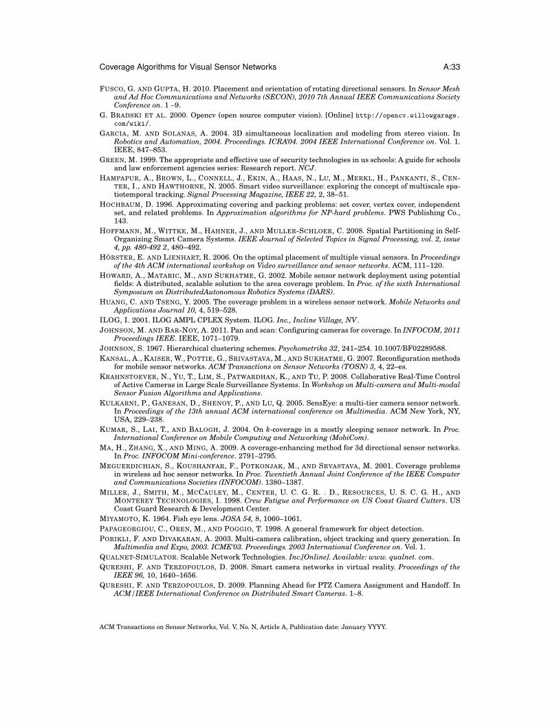
Coverage Algorithms for Visual Sensor Networks A:33
FUSCO, G. AND GUPTA, H. 2010. Placement and orientation of rotating directional sensors. In Sensor Meshand Ad Hoc Communications and Networks (SECON), 2010 7th Annual IEEE Communications SocietyConference on. 1 –9.
G. BRADSKI ET AL. 2000. Opencv (open source computer vision). [Online] http://opencv.willowgarage.com/wiki/.
GARCIA, M. AND SOLANAS, A. 2004. 3D simultaneous localization and modeling from stereo vision. InRobotics and Automation, 2004. Proceedings. ICRA’04. 2004 IEEE International Conference on. Vol. 1.IEEE, 847–853.
GREEN, M. 1999. The appropriate and effective use of security technologies in us schools: A guide for schoolsand law enforcement agencies series: Research report. NCJ.
HAMPAPUR, A., BROWN, L., CONNELL, J., EKIN, A., HAAS, N., LU, M., MERKL, H., PANKANTI, S., CEN-TER, I., AND HAWTHORNE, N. 2005. Smart video surveillance: exploring the concept of multiscale spa-tiotemporal tracking. Signal Processing Magazine, IEEE 22, 2, 38–51.
HOCHBAUM, D. 1996. Approximating covering and packing problems: set cover, vertex cover, independentset, and related problems. In Approximation algorithms for NP-hard problems. PWS Publishing Co.,143.
HOFFMANN, M., WITTKE, M., HAHNER, J., AND MULLER-SCHLOER, C. 2008. Spatial Partitioning in Self-Organizing Smart Camera Systems. IEEE Journal of Selected Topics in Signal Processing, vol. 2, issue4, pp. 480-492 2, 480–492.
HORSTER, E. AND LIENHART, R. 2006. On the optimal placement of multiple visual sensors. In Proceedingsof the 4th ACM international workshop on Video surveillance and sensor networks. ACM, 111–120.
HOWARD, A., MATARIC, M., AND SUKHATME, G. 2002. Mobile sensor network deployment using potentialfields: A distributed, scalable solution to the area coverage problem. In Proc. of the sixth InternationalSymposium on DistributedAutonomous Robotics Systems (DARS).
HUANG, C. AND TSENG, Y. 2005. The coverage problem in a wireless sensor network. Mobile Networks andApplications Journal 10, 4, 519–528.
ILOG, I. 2001. ILOG AMPL CPLEX System. ILOG. Inc., Incline Village, NV.JOHNSON, M. AND BAR-NOY, A. 2011. Pan and scan: Configuring cameras for coverage. In INFOCOM, 2011
Proceedings IEEE. IEEE, 1071–1079.JOHNSON, S. 1967. Hierarchical clustering schemes. Psychometrika 32, 241–254. 10.1007/BF02289588.KANSAL, A., KAISER, W., POTTIE, G., SRIVASTAVA, M., AND SUKHATME, G. 2007. Reconfiguration methods
for mobile sensor networks. ACM Transactions on Sensor Networks (TOSN) 3, 4, 22–es.KRAHNSTOEVER, N., YU, T., LIM, S., PATWARDHAN, K., AND TU, P. 2008. Collaborative Real-Time Control
of Active Cameras in Large Scale Surveillance Systems. In Workshop on Multi-camera and Multi-modalSensor Fusion Algorithms and Applications.
KULKARNI, P., GANESAN, D., SHENOY, P., AND LU, Q. 2005. SensEye: a multi-tier camera sensor network.In Proceedings of the 13th annual ACM international conference on Multimedia. ACM New York, NY,USA, 229–238.
KUMAR, S., LAI, T., AND BALOGH, J. 2004. On k-coverage in a mostly sleeping sensor network. In Proc.International Conference on Mobile Computing and Networking (MobiCom).
MA, H., ZHANG, X., AND MING, A. 2009. A coverage-enhancing method for 3d directional sensor networks.In Proc. INFOCOM Mini-conference. 2791–2795.
MEGUERDICHIAN, S., KOUSHANFAR, F., POTKONJAK, M., AND SRVASTAVA, M. 2001. Coverage problemsin wireless ad hoc sensor networks. In Proc. Twentieth Annual Joint Conference of the IEEE Computerand Communications Societies (INFOCOM). 1380–1387.
MILLER, J., SMITH, M., MCCAULEY, M., CENTER, U. C. G. R. . D., RESOURCES, U. S. C. G. H., ANDMONTEREY TECHNOLOGIES, I. 1998. Crew Fatigue and Performance on US Coast Guard Cutters. USCoast Guard Research & Development Center.
MIYAMOTO, K. 1964. Fish eye lens. JOSA 54, 8, 1060–1061.PAPAGEORGIOU, C., OREN, M., AND POGGIO, T. 1998. A general framework for object detection.PORIKLI, F. AND DIVAKARAN, A. 2003. Multi-camera calibration, object tracking and query generation. In
Multimedia and Expo, 2003. ICME’03. Proceedings. 2003 International Conference on. Vol. 1.QUALNET-SIMULATOR. Scalable Network Technologies. Inc.[Online]. Available: www. qualnet. com.QURESHI, F. AND TERZOPOULOS, D. 2008. Smart camera networks in virtual reality. Proceedings of the
IEEE 96, 10, 1640–1656.QURESHI, F. AND TERZOPOULOS, D. 2009. Planning Ahead for PTZ Camera Assignment and Handoff. In
ACM/IEEE International Conference on Distributed Smart Cameras. 1–8.
ACM Transactions on Sensor Networks, Vol. V, No. N, Article A, Publication date: January YYYY.
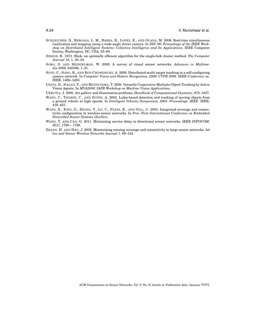
A:34 V. Munishwar et al.
SCHLEICHER, D., BERGASA, L. M., BAREA, R., LOPEZ, E., AND OCANA, M. 2006. Real-time simultaneouslocalization and mapping using a wide-angle stereo camera. In DIS ’06: Proceedings of the IEEE Work-shop on Distributed Intelligent Systems: Collective Intelligence and Its Applications. IEEE ComputerSociety, Washington, DC, USA, 55–60.
SIBSON, R. 1973. Slink: an optimally efficient algorithm for the single-link cluster method. The ComputerJournal 16, 1, 30–34.
SORO, S. AND HEINZELMAN, W. 2009. A survey of visual sensor networks. Advances in Multime-dia 2009, 640386, 1–21.
SOTO, C., SONG, B., AND ROY-CHOWDHURY, A. 2009. Distributed multi-target tracking in a self-configuringcamera network. In Computer Vision and Pattern Recognition, 2009. CVPR 2009. IEEE Conference on.IEEE, 1486–1493.
UKITA, N., NAGAO, T., AND MATSUYAMA, T. 2000. Versatile Cooperative Multiple-Object Tracking by ActiveVision Agents. In MVA2000, IAPR Workshop on Machine Vision Applications.
URRUTIA, J. 2000. Art gallery and illumination problems. Handbook of Computational Geometry, 973–1027.WANG, C., THORPE, C., AND SUPPE, A. 2003. Ladar-based detection and tracking of moving objects from
a ground vehicle at high speeds. In Intelligent Vehicles Symposium, 2003. Proceedings. IEEE. IEEE,416–421.
WANG, X., XING, G., ZHANG, Y., LU, C., PLESS, R., AND GILL, C. 2003. Integrated coverage and connec-tivity configuration in wireless sensor networks. In Proc. First International Conference on EmbeddedNetworked Sensor Systems (SenSys).
WANG, Y. AND CAO, G. 2011. Minimizing service delay in directional sensor networks. IEEE INFOCOM,2011, 1790 – 1798.
ZHANG, H. AND HAO, J. 2005. Maintaining sensing coverage and connectivity in large sensor networks. Adhoc and Sensor Wireless Networks Journal 1, 89–124.
ACM Transactions on Sensor Networks, Vol. V, No. N, Article A, Publication date: January YYYY.