Embed Size (px)
Citation preview
Scholars' Mine Scholars' Mine
Doctoral Dissertations Student Theses and Dissertations
Fall 2014
A contingency base camp framework using model based systems A contingency base camp framework using model based systems
engineering and adaptive agents engineering and adaptive agents
Dustin Scott Nottage
Follow this and additional works at: https://scholarsmine.mst.edu/doctoral_dissertations
Part of the Systems Engineering Commons
Department: Engineering Management and Systems Engineering Department: Engineering Management and Systems Engineering
Recommended Citation Recommended Citation Nottage, Dustin Scott, "A contingency base camp framework using model based systems engineering and adaptive agents" (2014). Doctoral Dissertations. 2352. https://scholarsmine.mst.edu/doctoral_dissertations/2352
This thesis is brought to you by Scholars' Mine, a service of the Missouri S&T Library and Learning Resources. This work is protected by U. S. Copyright Law. Unauthorized use including reproduction for redistribution requires the permission of the copyright holder. For more information, please contact [email protected].


A CONTINGENCY BASE CAMP FRAMEWORK
USING MODEL BASED SYSTEMS ENGINEERING
AND ADAPTIVE AGENTS
by
DUSTIN SCOTT NOTTAGE
A DISSERTATION
Presented to the Faculty of the Graduate School of the
MISSOURI UNIVERSITY OF SCIENCE AND TECHNOLOGY
In Partial Fulfillment of the Requirements for the Degree
DOCTOR OF PHILOSOPHY
in
SYSTEMS ENGINEERING
2014
Approved
Steven Corns, Advisor
Elizabeth Cudney
Hank Pernicka
Brian Smith
Suzanna Long
Kurt Kinnevan


iii
ABSTRACT
This research investigates the use of adaptive agents and hybridization of those
agents to improve resource allocation in dynamic systems and environments. These
agents are applied to contingency bases in an object oriented approach utilizing Model-
based Systems Engineering (MBSE) processes and tools to accomplish these goals.
Contingency bases provide the tools and resources for the military to perform missions
effectively. There has been increasing interest in improving the sustainability and
resilience of the camps, as inefficiencies in resource usage increases. The increase in
resource usage leads to additional operational costs and added danger to military
personnel guarding supply caravans.
The MBSE approach alleviates some of the complexity of constructing a model of
a contingency base, and allows for the introduction of 3rd
party analysis tools through the
XML metadata interchange standard. This approach is used to create a virtual
environment for the agents to learn the system patterns and behaviors within the system.
An agent based approach is used to address the dynamic nature of base camp operations
and resource utilization. , helping with extensibility and scalability issues since larger
camps have a very high computation load. To train the agents to adjust to base camp
operations, an evolutionary algorithm was created to develop the control mechanism.
This allows for a faster time to convergence for the control mechanisms when a change is
observed. Results have shown a decrease in resource consumption of up to 20% with
respect to fuel usage, which will further help reduce base costs and risk.

iv
ACKNOWLEDGMENTS
I would like to thank Dr. Corns for introducing me to the world of Systems
Engineering. Thank you for the guidance through my graduate studies and opportunities
to succeed in this field.
I would like to thank Dr. Pernicka for allowing me the chances to try and apply
some of the Systems Engineering processes to the satellite design team, giving me even
better insight into the processes. I would like thank Dr. Cudney, Dr. Smith, and Dr. Long
for helping and allowing me to move on the next stage of my life.
I would like my colleagues at CERL, Kurt and Ahmet, for giving me the
opportunity with ORISE and then eventually hiring me full time. Thank you for all of the
interesting projects that would eventually coalesce into my final research project.
Finally, I would like to thank Argentina for pushing me out of the door everyday
to get me to finish my research and writing. Thanks for sticking through the process with
me and explaining the jokes as I slowly stopped understanding everything outside of my
research. Thanks to Livy and Ari for giving me reasons to laugh and have fun. Thank you
to my family for all of the support through my longer-than-expected college career. I said
I would finish…eventually.

v
TABLE OF CONTENTS
Page
ABSTRACT ....................................................................................................................... iii
ACKNOWLEDGMENTS ................................................................................................. iv
LIST OF ILLUSTRATIONS ............................................................................................ vii
LIST OF TABLES ............................................................................................................. ix
SECTION
1. INTRODUCTION ...................................................................................................... 1
2. BACKGROUND AND PREVIOUS RESEARCH .................................................... 6
2.1. CONTINGENCY BASING ................................................................................ 6
2.2. DETAILED COMPONENT ANALYSIS MODEL ........................................... 9
2.2.1. DCAM Model ......................................................................................... 10
2.2.2. DCAM Conclusion ................................................................................. 14
3. MBSE BACKGROUND .......................................................................................... 16
3.1. MBSE METHODOLOGIES ............................................................................ 18
3.2. SYSTEMS MODELING LANGUAGE ........................................................... 19
3.3. MBSE INTEROPERABILITY ......................................................................... 20
4. CONTINGENCY BASING FRAMEWORK .......................................................... 22
4.1. MATHEMATICAL MODEL ........................................................................... 22
4.2. SYSML MODEL .............................................................................................. 23
4.2.1. System Domain ...................................................................................... 24
4.2.2. Modeling the Architecture ...................................................................... 25
4.2.3. Identification of Interactions .................................................................. 29
4.3. CREATE CANDIDATE SYSTEMS ................................................................ 30
4.3.1. Modeling Interactions ............................................................................. 31
4.4. MBSE MODEL ANALYSIS ............................................................................ 35
4.5. MBSE CONCLUSIONS ................................................................................... 38
4.6. APPLICATION TO STUDENT DESIGN TEAM ........................................... 42
4.6.1. Requirements .......................................................................................... 43
4.6.2. Physical System ...................................................................................... 45

vi
4.6.3. Mission Modeling ................................................................................... 47
4.6.4. Analysis .................................................................................................. 50
5. AGENT BASED MODEL ....................................................................................... 52
5.1. AGENT-BASED MODELING BACKGROUND ........................................... 54
6. AGENT SIMULATION ........................................................................................... 59
6.1. AGENT INPUTS .............................................................................................. 59
6.2. SIMULATION SPECIFICS ............................................................................. 61
6.3. CREATING A BASELINE MODEL ............................................................... 63
6.4. ADAPTABLE ARCHITECTURE ................................................................... 66
7. EVOLVING AGENTS ............................................................................................. 71
7.1. EVOLUTIONARY ALGORITHMS ................................................................ 71
7.1.1. Evolutionary Algorithm Parameters ....................................................... 73
7.2. AGENT INPUTS/OUTPUTS ........................................................................... 74
7.3. EVOLVING AGENTS EXAMPLE ................................................................. 77
8. CONCLUSION ........................................................................................................ 84
9. FUTURE WORK ..................................................................................................... 87
9.1. EVOLVING WITH GP-AUTOMATA ............................................................ 87
9.2. GP-AUTOMATA DEVELOPMENT ............................................................... 90
9.3. HYBRIDIZATION ........................................................................................... 93
BIBLIOGRAPHY ............................................................................................................. 95
VITA. .............................................................................................................................. 101

vii
LIST OF ILLUSTRATIONS
Page
Figure 2.1. Specify Soldier groups and their schedules in DCAM. .................................. 11
Figure 2.2. Specify the system configuration in DCAM. ................................................. 12
Figure 2.3. Expected use matrix for Soldier behavior in DCAM. .................................... 13
Figure 2.4. Specifying operational profiles of components and temperature in
DCAM. ........................................................................................................... 13
Figure 3.1. Foundation of OOSEM [Estefan, 2008]. ........................................................ 19
Figure 3.2. SysML Diagram Types................................................................................... 20
Figure 4.1. Contingency Base Domain Diagram. ............................................................. 25
Figure 4.2. Generalization of facilities into facility types. ............................................... 27
Figure 4.3. Block definition diagram of the dining facility showing
resources and components. ............................................................................ 29
Figure 4.4. Using model libraries to store objects for use in creation of
contingency bases. .......................................................................................... 31
Figure 4.5. Internal block diagram showing flows within the dining facility................... 32
Figure 4.6. Generators’ physical architecture at the camp level. ...................................... 33
Figure 4.7. Parametric diagram determining the total resource
usages/consumptions of the dining facility. .................................................. 33
Figure 4.8. Parametric diagram determining the total resource
usages/consumptions of the contingency base. ............................................. 34
Figure 4.9. Screen capture of the GUI tool that utilizes model data. ................................ 36
Figure 4.10. Transition from documented requirements to model requirements. ............ 45
Figure 4.11. Block diagram of satellite subsystems. ........................................................ 46
Figure 4.12. Block definition diagrams for (a) ADAC structural
composition and (b) Magnetometer specification. ....................................... 47
Figure 4.13. Use case diagram showing the use case linked with an
activity diagram. ........................................................................................... 48
Figure 4.14. Behavioral analysis showing (left) Operational Modes of the
satellite and (right) Initialization Mode activities. ....................................... 49
Figure 4.15. Theoretical user interface for satellite totals analysis. .................................. 51
Figure 5.1. Properties of agents [Macal, 2006]. ................................................................ 55
Figure 6.1. Architecture of the baseline agent model. ...................................................... 64

viii
Figure 6.2. Generator 1 power profile with connected system and
soldier group. ................................................................................................. 64
Figure 6.3. Generator 2 power profile with connected system and
soldier group. ................................................................................................. 65
Figure 6.4. Generator 3 power profile with connected system and
soldier group. ................................................................................................. 65
Figure 6.5. Generator 4 power profile with new connected systems
and soldier group. .......................................................................................... 68
Figure 7.1. Possible inputs and responses of a generator agent. ....................................... 75
Figure 7.2. Initial Soldier groups’ schedules. ................................................................... 80
Figure 7.3. Optimal Soldier groups’ schedules ................................................................. 81
Figure 7.4. Initial Systems’ Power Usages. ...................................................................... 81
Figure 7.5. Optimal Systems’ Power Usages.................................................................... 82
Figure 7.6. Initial Generator 1 Properties. ........................................................................ 82
Figure 7.7. Optimal Generator 1 Properties. ..................................................................... 83

ix
LIST OF TABLES
Page
Table 4.1. Total resources required or produced given the alternative cases. .................. 37
Table 6.1. Approximate Diesel Fuel Consumption Chart (provided by
Diesel Service and Supply) .............................................................................. 62
Table 6.2. Initial Configuration Daily Fuel Usage. .......................................................... 66
Table 6.3. Solution scoring table for each possible generator configuration .................... 67
Table 6.4. New Configuration Daily Fuel Usage. ............................................................ 68
Table 6.5. Unoptimized and optimized fuel usages of a 3 tent addition
to the model. ..................................................................................................... 70
Table 9.1. Genetic Programming Operators Syntax ......................................................... 91
Table 9.2. Finite State Machine Response Scheme. ......................................................... 91
Table 9.3. Genetic Programming Terminal Descriptions. ................................................ 92
Table 9.4. Example of a GP-Automata controller with states, transition,
and decider information. .................................................................................. 92
1. INTRODUCTION
The United States faces profound challenges that require strong, agile, and
capable military forces whose actions are harmonized with other elements of U.S.
national power. The balance between available resources and our security needs has
never been more delicate [Office of the Secretary of Defense, 2013].
In the mid to long term, U.S. military forces must plan and prepare to prevail in a
broad range of operations that may occur in multiple theaters in overlapping timeframes.
This includes maintaining the ability to prevail against two capable nation-state
aggressors, but the need to plan must be taken seriously for the broadest possible range of
operations – from homeland defense and defense support to civil authorities, to
deterrence and preparedness missions – occurring in multiple and unpredictable
combinations [Office of the Secretary of Defense, 2010]. In many instances, the need to
conduct extended operations over time has resulted in U.S. forces remaining in these
areas far longer than initially anticipated. Often temporary locations (such as bivouac
sites and assembly areas) evolve into enduring base camps [TRADOC, 2009] to support
changing mission requirements.
Over the next quarter century, U.S. military forces will be continually engaged in
some dynamic combination of combat, security, engagement, and relief and
reconstruction [United States Joint Forces Command, 2010]. The current national
strategies and Joint Operating Environment (JOE) indicate a strong likelihood of long-
term military commitments abroad to achieve national goals with respect to the overseas
contingency operations. These operations have different basing needs that are mission

2
dependent, so as the operational requirements change the capabilities of the base camp
must change to support those operations.
The future Modular Force will be a campaign quality expeditionary force that
supports the nation by conducting full spectrum operations in a joint, interagency,
intergovernmental, and multinational environment within the context of the JOE. Land
forces may be deployed in the continental U.S. (CONUS) or outside CONUS (OCONUS)
in a range of environments from austere to urban and for short to extended periods of
time. Contingency bases represent the physical standpoint in a deployed location from
which operations are projected or supported. In essence, they are the physical locations
supporting power projection for the operational force in the theater of operations
[TRADOC, 2009]. The term power projection is used to emphasize that a contingency
base is the physical location within the operational area that enables power projection.
These bases sustain civil as well as the military components of U.S. national power to
rapidly and effectively respond to crises, contribute to deterrence, and enhance regional
stability. The U.S. Army does not currently have the capability to address contingency
base issues arising from these dynamic demands, and so new systems based approaches
must be explored to provide these capabilities.
A system level approach of modeling is necessary as contingency bases must
provide all equipment, facilities, and personnel required to support a specified number of
troops and mission. Because of the diversity of environments, personnel, and mission
types and durations, no two contingency bases will exactly be the same. Changes to any
contingency base parameters will cause a change in the structure and requirements of that
contingency base, and changes can occur at any time with no warning.

3
Another factor increasing the complexity of contingency base design is that each
facility type can have multiple structural type options ranging from tents to pre-existing
buildings, and each building construction type will have different utility requirements.
Knowing the total resources required to keep a camp operational allows logistics to be
planned and anticipated to provide base sustainment. Many of the overall daily utility
consumptions or productions are estimations and vary depending on the source of
information. Water consumption can vary from 25 gallons to 60 gallons of water per day
per soldier [Noblis, 2010]. The project this work is derived from also looks at utility
estimations for each individual facility. Many of the values are estimated and verified by
people familiar with operational bases. Issues arise with planning larger bases because
they could include facilities and systems that provide services that impact a Soldier’s
quality of life, which in return impact the requirements for base sustainment. For
example, larger bases tend to provide more “convenience” power to Soldiers for use in
their billeting areas. Therefore, depending on the Soldier activity, each billet could have a
different power load on the overall base.
Contingency bases contain many different, independent entities with many
interactions. This adds to the complexity of the entire system and increases the number of
resources necessary for modeling and simulating the design. A model that includes all
components and interactions will typically end up with better designs, but may not be
resource efficient. There is typically a trade-off between design detail and the return from
the effort of adding the detail, known as value-of-information [Panchal et al, 2009]. The
effort and time spent on detailing an entire contingency base would be limitless due to the
ad-hoc nature of bases and their components.

4
The projects discussed in this research all take an object-oriented approach to
modeling a contingency base. The first project models the facilities as abstract objects
that represent the facilities as functions. The purpose of this model is to give an initial,
rough estimate of a base to provide DoD designers and contingency base personnel
information about the efficacy of a design. The model was developed in a Model-based
Systems Engineering tool. The information is then exported into a standalone tool
referred to as the Resource Calculator to give the user a highly configurable environment
to examine a base’s daily logistical loads. It is very high-level evaluation that gives a
general idea of resource loads based on number of soldiers and temperature category.
Using this method, a generalized view of the base camp is examined and an acceptable
solution can quickly be provided. Once a simplified design exhibits beneficial solutions,
additional details can be added to elaborate on the design.
In 2011, The Department of Defense also released their first Operational Energy
Strategy. Among its goals, it calls for a reduction in the demand for energy in military
operations [Operational Energy, 2011]. One method of reduction is to look at the
contingency bases and find new technologies or processes to introduce into bases.
Putnam created a model to simulate a small, 150-person basing kit. In this model, he is
able to simulate components on a second-by-second basis [Putnam, 2012]. The
components are either existing ones currently part of the kit, or potential components
looking to replace the older models or fill a capability gap. New, potential technologies
are looked at by Technology Enabled Capability Demonstrations (TECDs) 4a working
group. TECDs look at the seven “Big Army Problems”, which includes Army Problem 4
[Freeman, 2011]:

5
“We spend too much time and money on STORING, TRANSPORTING,
DISTRIBUTING and WASTE HANDLING of consumables (water, fuel,
power, ammo and food) to field elements, creating exposure risks and
opportunities for operational disruption.”
The 4a working group primarily focuses on basing capabilities. They required
modeling and simulation tools in order to evaluate projects in a basing environment. One
of the tools looking to be used is the Detailed Component Analysis Model (DCAM),
which is based on Dr. Putnam’s work. More background on DCAM will be presented in
Section 2.
The Resource Calculator is extensible but not detailed, and DCAM is detailed but
has challenges with extensibility. They also both represent steady-state analysis, and do
not perform any failure analysis or change of state analysis. The method proposed to
overcome these issues is by making an agent-based model of the contingency base with
the facilities acting as agents. The benefits are better extensibility in order to model larger
camps or even more permanent installations, and better represent the interactions between
components in a more realistic way. The agents can also be programmed to adapt their
behavior response in order to optimize their logistic schedule or network, further
reducing their logistical demand. The agent model and background on why agents were
chosen is in Section 5.

6
2. BACKGROUND AND PREVIOUS RESEARCH
2.1. CONTINGENCY BASING
The U.S. Department of Defense (DoD) has recently implemented policy
specifically addressing contingency base camp design and operations [Department of
Defense, 2013]. The new DoD policy pursues increased effectiveness and efficiency in
contingency basing by:
a. Promoting scalable interoperable capabilities that support joint, interagency,
intergovernmental, and multinational partners.
b. Providing common standards for planning, design, and construction in accordance
with the Under Secretary of Defense for Acquisition, Logistics, and Technology
(USD (AT&L)) Memorandum for developing common standards for contingency
services; and establishing standards for equipment, base operations, and base
transition or closure.
c. Using operational energy efficiently in accordance with the guidance stated in the
DoD Operational Energy Strategy and DoD Directives (DoDDs) 5134.15 and
4140.25, minimizing waste, and conserving water and other resources.
d. Integrating comprehensive risk management for emergency management,
environment, safety, explosives safety, occupational health, and pest management
into planning, design, and operations in accordance with paragraph 4.3. of DoDD
4715.1E and for security in accordance with DoDD 5200.43.
e. Minimizing the logistics footprint by optimizing the delivery of materiel
solutions, contracting practices, and services.

7
f. Providing the appropriate mix of military, civilian, and contractor personnel
competencies in the DoD Total Force planning process in accordance with
paragraph 4c of DoDD 1404.10 and the guidance in DoD Instruction (DoDI)
1100.22.
g. Conducting contingency basing education and training for military and civilian
personnel in accordance with paragraph 4.1.4. of DoDD 5124.02 paragraph 4a of
DoDD 1322.18.
h. Minimizing adverse impacts on local populations and cultural resources.
Depending on the number of Soldiers (approximately), the contingency bases can
be classified as one of multiple types: a Patrol Base (PB) for 150 Soldiers, Combat
Outpost (COP) for 300 Soldiers, Forward Operating Base (FOB) for 1000 Soldiers, or
Super FOB for up to 6000 Soldiers. The stated populations account for the operational
Soldiers performing missions and not the contractors or support troops performing duties
on the camp. Bases must also take into account any other bases they are supporting,
which will need to be continuously provided with supplies and equipment. Each FOB
may have multiple COPs that it has to help keep supplied, and additionally each COP
may have to supply multiple patrol bases.
A contingency base can have more than 40 possible facility types implemented as
part of the base, depending on the base size. Each type performs a different function for
the base. In a base, there may also be multiple instances of facility types. For example,
there would likely be multiple housing facilities to accommodate the population of the
base. A contingency base can be built by selectively building various combinations of
these facilities at various construction standards depending on the planned level of
8
capability of the base. The level of capability of a contingency base as defined by the
DoD [Department of the Army, 2013] includes:
Basic capability camps utilize facilities to establish initial entry using organic
capabilities and prepositioned stocks. Basic capabilities are those functions and
services that are considered essential for sustaining operations for a minimum of
60 days and include necessities like protection, sleeping, hygiene, eating, and
provide operationally dependent resources like motor pool or tactical operations
center. Basic facilities and infrastructure are highly flexible and moveable (e.g.
tents vs. fixed or constructed structures),
Expanded capabilities are basic capabilities that have been improved to increase
efficiencies and intended to sustain operations for a minimum of 180 days.
Expanded capabilities may include optional support facilities such as chapels,
education centers, fitness centers, etc., which provide for the soldiers’ morale,
welfare, and recreation.
Enhanced capabilities, which are expanded capabilities that have been improved
to operate at optimal efficiency and can support operations for an unspecified
duration. At this level of capability, contingency base facilities start resembling
their counterparts in permanent bases or installations.
The most common and standard of these facility types are taken mostly from
prominent contingency basing standards reports, commonly known as the “Red Book”
[United States Army, 2004] and the “Sand Book” [USCENTCOM, 2007].
There are some tools available to aid in the design of contingency basing
solutions, such as the Theater Construction Management System (TCMS) and the
9
Geographical Base Engineer Support Tool (GeoBEST). TCMS is a tool used for
computer-aided “planning, design, and management of contingency construction mission
in a theater of operations and for emergency construction support during disaster relief
operations [United States Army, 2011].” The tool contains a repository of facility
designs, component designs, and some base camp designs. One of the drawbacks found
with the system is the lack of life cycle analysis of the base camps [Marlart, 2003]. In
addition, it does not provide a means for examining the interactions between the base
camp components, and also lacks an ability to analyze utility requirements like power,
water, and waste. GeoBEST was a separately developed decision support tool for base
camp planning developed by the US Army Engineer Research and Development Center
(ERDC) and the Air Force. It was designed to integrate with many existing tools
including ArcGIS to give georectified information on proposed base locations. GeoBEST
was utilized to provide a three dimensional visualized base camp layout and help with
spacing requirements between facilities [Williams, 2002]. However, GeoBEST does not
capture the underlying engineering information relating to the required resources of the
base camp.
2.2. DETAILED COMPONENT ANALYSIS MODEL
The detailed component analysis model (DCAM) and tool were adapted from
research performed by Putnam [2012]. The goal of the research was to make a realistic
model of a contingency base, specifically the 150-man Force Provider kit. The Force
Provider kit is a set of known components that are sent to the site location. As opposed to
the generalized nature of the MBSE method, the Force Provider kit is certain, observable,
and repeatable, lending itself to an initial evaluation. Another goal was to find resource-

10
saving designs by either altering the architecture like reducing the number of generators
to increase their efficiency and use less fuel, or introduce improved technologies or
capabilities into the kit. DCAM has expanded the scope past the Force Provider kit, but is
still limited in scope to lack of operational and baseline data of components.
2.2.1. DCAM Model. The model once operated on MATLAB, but now resides
in both an Excel format and a hand coded database method with GUI. The DCAM model,
like the MBSE method, uses an object oriented approach. The type of systems and their
major components modeled currently are latrines, laundry, kitchen and dining, showers,
billeting tents, and shower water reuse system. For a detailed look at the systems,
specifically Force Provider systems, see [Putnam, 2012]. The components do not go
down to a detailed level. For example, there is no modeling of electrical wires or
plumbing. The components are kept abstract and treated as black boxes during the
analysis. The types of components are distinguished from each using a component code.
For example, a component code 6 is for water flow within the latrines and showers, and a
component code 1 may deal with an electrical component (the actual component codes
are still in development and subject to change.) The component code determines which
component attributes are important for the analysis. Each component is an object that
contains specific attributes for its function and a “mode profile.” The “mode” of the
component is determined by the time step in the profile corresponding to the same time
step in the simulation. These mode profiles are specific to the component. There are other
environment profiles that apply to some or all components. Those include the operational
profiles of the military units and temperature profile of the location.
11
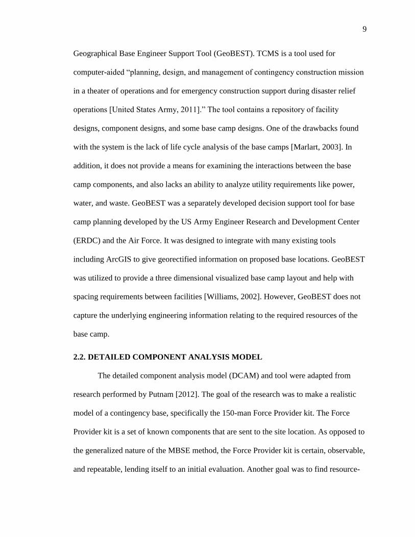
For the database variation, the components and attributes are stored in a database.
These default components cannot be directly changed by the end user. The first step for
the end user is specifying the military units, the number of members per unit, and their
daily schedule. The members can be ‘On Duty On Base’, ‘On Duty Off Base’, or ‘Off
Duty On Base’ (Figure 2.1).
Figure 2.1. Specify Soldier groups and their schedules in DCAM.
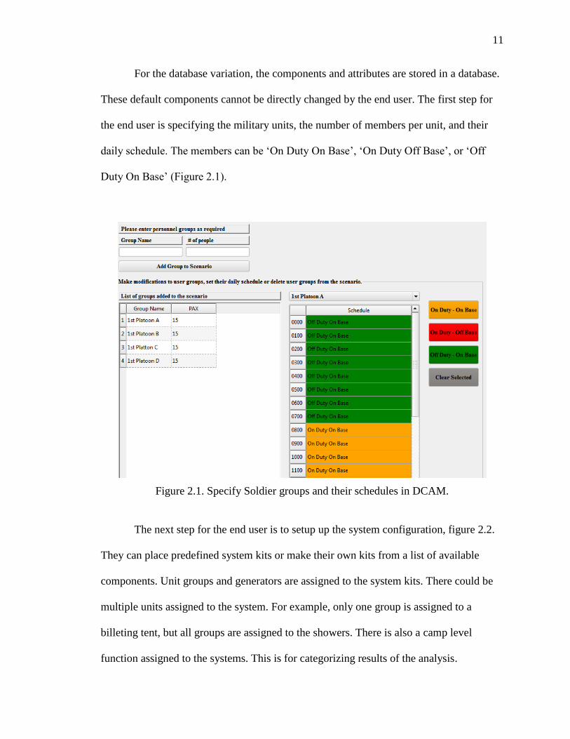
The next step for the end user is to setup up the system configuration, figure 2.2.
They can place predefined system kits or make their own kits from a list of available
components. Unit groups and generators are assigned to the system kits. There could be
multiple units assigned to the system. For example, only one group is assigned to a
billeting tent, but all groups are assigned to the showers. There is also a camp level
function assigned to the systems. This is for categorizing results of the analysis.

12
Figure 2.2. Specify the system configuration in DCAM.
The expected use matrix (figure 2.3) is updated in the next step. These are for any
place components that have a usage event associated with them. They follow the discrete
event method closely in that they do not function unless acted upon, whereas other hotel
load components like the lights operate are modeled as continuous loads. These are
mostly latrine and shower based components, as well as personal electronics. They rely
on a person to initiate their use and are more stochastic rather than deterministic as
specified by the mode profile. Putnam specified the likelihood that a person will initiate
the usage event per day depending on their current operation profile state [Putnam, 2012].
This likelihood is only applied to the times the person is on base. The longer the person is
on base, the lower the percentage of initiating the event because they have more time
available.

13
Figure 2.3. Expected use matrix for Soldier behavior in DCAM.
The last step is to apply the temperature and mode profiles, see figure 2.4. Both
are user configurable. The temperature profile specifies the temperature on an hourly
basis. The time step could be reduced given there is data available at that level of fidelity.
The mode profile is for the deterministic components that have more of a continuous
behavior. It is a simple binary array. One (1) represents the ‘ON’ state for the component,
and Zero (0) represents the ‘OFF’ state. Profiles could be setup however the end user
desires. Common mode profiles are ‘ON 24-hours per day’, ‘ON 8 hours night’, or ‘ON 3
Meals’. These are only applied to the components and not the parent system kit.
Figure 2.4. Specifying operational profiles of components and temperature in DCAM.
14
The analysis portion of DCAM is discretized into one second time steps. The
simulation is run to represent a single day, or 86,400 seconds. The analysis is split into
two functions. The first function generates an array of the resource demand averaged over
a minute for each component except for the generators. Then, any component that has an
electrical load is evaluated by the second function to determine the electrical supply
model using the resource demand array generated in the first function. The supply model
determines the fuel consumption of the generators for their given loads and if all of the
loads are able to be met.
2.2.2. DCAM Conclusion. DCAM does a good job of balancing value of
information. It can simulate the Force Provider kit accurately without having to
use valuable modeling and computation resources to put fine details on all the
components. It is a simple, object-oriented model that requires “only a small number of
parameters…for each component” [Putnam, 2012]. Given the correct information, new
components could be added into the model, and have been added since the research was
published. It fits nicely in the MBSE method. The blocks would represent the
components and systems, and analysis run through an external program.
With all models, there are areas that could be changed to improve or alter
function. One of the main issues at the moment with DCAM is the high computational
resources it requires in time and processing power. There is also desire from the end users
to have simulations longer than a day. With each component at a one-second time step,
the analysis time can get very large. Dr. Putnam does note that not all of the components
require a one-second time step. Potable water, waste water, solid waste “do not require a
1-minute time step to develop accurate estimations” [Putnam, 2012]. They are stored in

15
containers that usually aren’t accessed at a repetition, usually every couple of days.
However, there are some electrical processes that take less than a minute to cycle. This is
the reason for the one-second time steps.
Also, special interactions, like where water flow affects power demand, handled
on a case-by-case basis. This could pose issues with extensibility if a new interaction is
needed. Since this modeling is being used to simulate projects presenting new
capabilities, it is possible for this problem to arise. Due to the way the simulation is
performed, any failure or abnormality would have to be randomly generated during the
making of the profile. This would prevent the simulation from having realistic failure
responses. The initial research did not call for failure or abnormal behavior to be
simulated. Both the MBSE model and DCAM represent a steady-state analysis. Now,
there is starting to be a request for unsteady-state analysis. In the MBSE model, we
observed many tertiary effects that were not always anticipated. With the more detailed
models, it would be beneficial to observe the effect as well. One component could affect
another, but there is no interaction of this kind in DCAM. There is also no way to
simulate the response since the abnormality is only in the use profile and it cannot
retrieve the generator response until after the use profile is generated. The generator will
need to be simulated alongside the other components.

16
3. MBSE BACKGROUND
The MBSE Initiative was started in 2007 during the International Council on
Systems Engineering (INCOSE) International Workshop. As part of the INCOSE SE
Vision 2020 statement, MBSE is “part of a long-term trend toward model-centric
approaches adopted by other engineering disciplines…(and) is expected to replace the
document-centric approach…by becoming fully integrated into the definition of systems
engineering processes [Crisp, 2007].” The MBSE environment is made up a modeling
language, tools, methods, and way to incorporate them all.
The MBSE approach was initially looked at and later pursued because of the
diversity and fluctuation involved in the design process. MBSE moves the document-
focused design approach into a single, computer model approach which supports
analysis, specification, design, verification, and validation of complex systems
[Friedenthal et al, 2009]. The purpose was to lay out a framework model of a contingency
base that can then be imported and utilized in engineering and planning tools, like the
Resource Calculator. In the model-based approach, contingency bases can be designed
easily and quickly. Different variations to the base can be modeled and compared against
each other. Many of the scenarios a base encounters can be modeled and analyzed before
construction starts, and because all the information is already in a computer format,
computer-aided analysis tools could be employed for detailed analysis. This allows
planners to conduct trade studies on different base designs, and get feedback on good or
bad design choices.
The lack of standards for equipment used in the expanded and enhanced
capabilities base camps necessitate a flexible approach for including model elements and

17
assess their effects on the overall base. If the information is modeled in an abstract and
consistent manner, then the system can be analyzed before actual components are even
selected. A more efficient generator or tent that requires less area could be implemented
into the model without having to remake any of the models. In addition, because the
relationships remain approximately the same, the model is applicable across the spectrum
of base sizes. Haiar et al. [Haiar et al, 2006] found that design and analysis could be
performed simultaneously by modeling objects in an abstract manner and later develop
the physical model as it was finalized. This allowed greater flexibility in design changes.
They also found that model-based engineering provides a way to reduce design cycle
time. This type of approach is beneficial for contingency base planning since the
environment that a contingency base operates is always changing and evolving.
Populations, missions, threat levels will never be constant. So any big changes could be
implemented on the model to anticipate changes required on the camp.
The use of a model-based systems engineering approach has also made it possible
to elicit parametric information from subject matter experts in the design of these
contingency bases. By using the visual data representation, it is easier to highlight
decision points and how the base camp elements interact in the model so that the subject
matter experts can detect and correct any errors. This makes it possible to provide a
validated tool for the creation of early design concepts for contingency basing, as well as
capturing knowledge and making it available to other personnel involved in contingency
basing design.
Model-based Systems Engineering approaches have been implemented on other
similar projects as well, like disaster management systems [Soyler and Sala-Diakanda,

18
2010] and planning in the industrial symbiosis domain [Sopha et al, 2010]. Industrial
symbiosis involves the exchange of resources between collaborating businesses. There
are also numerous challenge teams for using MBSE to solve particular problems in the
areas of Modeling and Simulation Interoperability, Space System Modeling, Telescope
Modeling, Biomedical Modeling, and GEOSS Modeling [OMG MBSE]. The Department
of Defense Architectural Framework (DoDAF) is brought into MBSE in order to offer
guidelines for project development and a way to build the model [Piaszczyk, 2011].
Much of the validation and verification plans are traced to views from DoDAF.
3.1. MBSE METHODOLOGIES
There are multiple MBSE methodologies that have been developed and adopted
including IBM Telelogic Harmony-SE, INCOSE Object-Oriented Systems Engineering
Method (OOSEM), IBM Rational Unified Process for Systems Engineering (RUP SE) for
Model-Driven Systems Development (MSDS), Vitech MBSE Methodology, and JPL
State Analysis [Estefan, 2008]. INCOSE’s Object-Oriented Systems Engineering Method
(OOSEM) has been selected for use on this project. Many of the methodologies have a
focus around software development and project management. OOSEM has objectives
that closely align with the processes looking to be used in this research. Like all of the
alternatives, a main objective of OOSEM is requirements and design analysis of the
system. However, the integration with object-oriented software and system-level reuse
and design evolution are where OOSEM stood out. OOSEM uses a traditional top-down
systems engineering approach with the Object Management Group’s Systems Modeling
Language™ (OMG SysML™). The core activities for development of a system include
analysis of stakeholder needs, definition of system requirements, definition of a logical

19
architecture, synthesis of candidate allocated architectures, optimization and evaluation
of the alternatives, and the validation and verification of the system [Estefan, 2008].
OOSEM utilizes systems engineering as a base, and builds upon it with some common
object-oriented techniques. Finally, it introduces unique techniques such as causal
analysis and requirements variation analysis (Figure 3.1) [Estefan, 2008].
Figure 3.1. Foundation of OOSEM [Estefan, 2008].
3.2. SYSTEMS MODELING LANGUAGE
SysML was developed for addressing Systems Engineering problems by the
Object Management Group (OMG) as an extension to the Unified Modeling Language
(UML). UML is widely used in software development for modeling software systems.
The language helps with architecting systems and specifying components of a system
through a graphical representation with a semantic base for structural composition,
behavior, constraints, and requirements, as well as the allocation between these
representations [OMG SysML]. SysML adds to the functionality of UML so that
engineers can model physical systems as well. As part of the additional functionality,

20
new diagrams were created and others modified from UML specifications, see figure 3.2.
The block definition diagram represents the “system hierarchy and system/component
classification,” and the internal block diagram “describes the internal structure of a
system in terms of its parts, ports, and connectors” [OMG SysML]. The parametric
diagram is used to describe the mathematical relationships with the system.
Figure 3.2. SysML Diagram Types.
3.3. MBSE INTEROPERABILITY
There are numerous ways of exchanging data between tools including manual
entry, file based exchange, interaction based exchange, and repository based exchange
[Friedenthal, 2009]. The manual method involves typing in the data in each tool
separately. A dual screen setup would be beneficial so each tool could have a screen to
display its information. This would end up being a very time consuming approach to data
exchange. The file based exchange uses applications that can understand similar file
types. This would be like document applications being able to open different formats like

21
.txt, .rtf, or .doc. The interaction based exchange needs a tool’s application programming
interface (API). The API allows other tools to access and filter its data. This method has
the most overhead and difficulty in terms of setup. The last method, repository based
exchange, uses a database accessible by multiple tools.
In SysML, all components a model can be represented as metadata. XMI is a file
based exchange method based on the industry standards XML, Meta Object Facility
(MOF), and UML. It is a set of rules for transforming model information into a unique set
of tags in XML [Friedenthal, 2009]. [Patel, et al., 2010] goes further into using the XMI
format to allow for executing SysML models. The information can also be transformed
for use by Modelica, as shown in [Paredis, et al., 2010]. A second model interchange
standard is ISO 10303 and its specific application protocol 233 (AP233). ISO 10303 is
also known as the Standard for the Exchange of Product Model Data, or STEP. It is an
international standard used to describe “describe product data throughout the life cycle of
a product, independent of any particular system” [Friedenthal, 2009]. AP233 was created
to support systems engineering, and was developed in coordination with SysML.
XML is a flexible text format developed for the exchange of information. It is
machine-readable while also being able to be easily understood by a person [Jones and
Drake, 2002]. It is also not tied to any specific software application. XML is organized in
a hierarchical structure made up elements. The elements can be specified by the user
under any name, or tag. This allows the user to create and organize data in a specific
manner. However, this also means any application using the data will have to know the
structure and tags of the data. These mappings of the data can be supplied by an
associated schema.

22
4. CONTINGENCY BASING FRAMEWORK
4.1. MATHEMATICAL MODEL
During the process of defining the system, 12 parameters are identified that can be
used to define the personnel and resource requirement and waste generation of each
facility. These parameters are: electricity required, fuel required, potable water required,
bottled water required, storage area, number of personnel to operate facility, gray water
produced, black water produced, solid waste produced, food required, footprint of
facility, maintenance hours per day.
Each parameter is estimated with a total consumption/production per day per
solider. Then, each facility’s parameter is given an estimate of the percentage it uses of
the total amount. Many of the values are derived from field manuals like the Sand Book
[USCENTCOM, 2007] and other reports [Noblis, 2010]. Other values are given using
engineering approximations until totals resemble anticipated totals. All values,
estimations and totals, are verified for general accuracy by subject matter experts familiar
with operational camps.
Each contingency base has an estimated usage per person per day for the different
parameters. In order to get the total utility resource requirements for each facility, the
usage values provided by the individual facilities for the individual parameters, base level
estimations, and initial amount of Soldiers are populated into a system of linear equations
and solved simultaneously. The mathematical model came from the iterative process of
applying engineering estimates to the facility usages and having them validated by
subject matter experts [Poreddy and Daniels, 2012].

23
It should be noted that the estimations for these parameters are not linearly
scalable. Values for the larger size camps will not always work for smaller camps. Each
value has an associated soldier population range it is accurate for. Also, some of the
smaller camp’s facilities have constants instead of percentages. For example, a dining
facility requires 2 personnel, regardless if there are 100 soldiers or 150 soldiers.
Parameter values will also differ by geographic location. A camp in the arctic or desert
will need more fuel to produce more electricity for heating or cooling. Meanwhile, a
camp in a moderate temperate zone will not require much power for heating and cooling.
4.2. SYSML MODEL
The model was developed studying a base with a population of roughly 600
Soldiers for missions and operations. The needs are defined by the mission objectives that
the contingency base must support. For the development of a contingency base
architecture and requirements, direct meetings were conducted with Department of
Defense personnel involved in the design of contingency bases to capture subject matter
expert input.
The requirements are derived from the capabilities established by the Army based
on the expected Joint Operational Environment (JOE). The general categories covered by
these requirements include planning and design, construction, operations, management,
and transfer and closure. The requirements that guide those categories (in a generalized
form) are:
The system shall minimize logistical requirements while maintaining operational
capabilities and readiness.
The system shall use modular, scalable, sustainable, and adaptable designs.

24
The system shall decrease construction and deconstruction requirements.
The system shall improve operational efficiencies in energy, water, and waste.
The contingency base systems’ interrelationships were decomposed in order to
ascertain the various links between the components and systems, as well as, the critical
nature of those relationships. In this way, system requirements were also assessed from a
risk perspective. This led to greater engagement with DoD planners and managers when
the base camp architecture was developed.
4.2.1. System Domain. The contingency base domain is modeled to account for
any factors that influences contingency bases as a whole, including internal influences,
external influences, and the relationship between them (Figure 4.1). Within the system
base camp perimeter, actors are used to represent Soldiers, civilian workers, vehicles, and
any other persons, organizations, or external systems that influence the system
[Friedenthal et al, 2009]. Actors are chosen as the method for modeling the system
impacts because they are able to act as consumers of utilities within the contingency base,
and are also able to leave the boundaries of the system. Alternatively, facilities are
represented as a single block within the contingency base domain, as they are unable to
leave the boundary of the system and act as components of a system. The facilities block
includes all of the facilities that make up the system. The environment, which include all
outside influences on the system, is represented by another block in figure 4.1. The
environment is made up of several parts, including other bases, enemy combatants,
weather, and the social/political environment within which the base must operate. The
influences of other bases would be associated with the requisite supplies and/or
Soldiers/Civilians necessary to maintain operational effectiveness, either at the existing

25
base or in those bases which the existing system supports. Enemy combatants affect the
methods of defense present on the base, the resupply timing, the mission operational
tempo, the unit types involved, the duration of missions, and the base designs. Weather
influences the type of structures and utilities necessary to meet operational requirements.
Social influences are local factors like customs, local labor availability, and locals’ image
of the base and Soldiers. Political influences affect the mission, duration, or special
directives. All of these influences affect utility requirements.
Figure 4.1. Contingency Base Domain Diagram.
4.2.2. Modeling the Architecture. There are two main methods to generate
candidate contingency bases for comparison in a trade study. The first is manually
creating and editing each facility type in the SysML modeling tool, altering values as
necessary, and saving a copy of the system. The second method is to create a model
library of blocks of facility types that have a specified range of populations for which

26
they are applicable, thereby creating a repository of options from which to build the base
camp. The first option is more of an exhaustive approach and would require creation of
the facilities each time a new contingency base is modeled. The second method leverage
several benefits of an MBSE approach and is the focus of this project.
To keep the model simple and adaptable, facilities are modeled as abstract objects
in a model library where utility requirements can be changed after placement in a model.
This is an object oriented approach where each facility is specialized from a generic
block. In this way, it is not necessary to model all possible variations of tents, structures,
or facilities found on a contingency base. For example, the dining facility is created as
just Dining. There is no differentiation such as “Tent, Type 1 Dining” or “Tent, Type 2
Dining” (Figure 4.2). This abstraction makes it possible to alter the utility requirements
of any object as necessary. Like the facilities, the generators on the base are also
generalized as ‘Electrical Generation’. This abstraction makes it possible to alter the
utility requirements of any object as necessary.
The first step is to create a package organization and hierarchy. Packages for each
facility are made and placed into their appropriate category. Packages for system actors
and facility variables are also created. This is similar to the domain diagram, but with
greater detail for the facility components and utilities. These packages include all
possible components and flows that could make up a base camp. The vehicles are
modeled as actors and block because they have the ability to enter and leave the
boundaries of the base camp. When the vehicles are within the boundaries, they will act
as like a facility consuming resources and producing waste. Creating them as blocks as
well is a way to show that dynamic role.

27
Figure 4.2. Generalization of facilities into facility types.
Next, ValueTypes of the different resource flows are created. ValueTypes are a
way to express properties of a component with user-specified units and dimensions. In
this example, the ValueTypes created have the units of the resource flow (e.g. Fuel would
be gallons) per person per day. Every ValueType is applied to the facility type blocks,
regardless of whether they consume or supply the flow (Figure 4.3). The default value for
each usage ValueType is set to the value defined in an associated mathematical model
[Poreddy and Daniels, 2012]. The mathematical model came from the iterative process of
applying engineering estimates to the facility usages and having them validated by
subject matter experts. If the facility does not consume or generate a flow then the default
value for that resource is set to zero. When the usage value is a constant, such as a facility
needing two personnel to operate no matter what the environment variables are, the ‘Is

28
Constant’ property is set to true. The actual resource requirements are not set until the
system is solved.
Finally, blocks are created for each of the facilities, and their ‘flows’ of the
resources and wastes. Blocks are a way to represent components of the system. Blocks
can be composed of other blocks. Blocks are created for each facility and the parameter
flows added to each block (Figure 4.3). Depending on the amount of details desired, parts
within a facility can be modeled as well. In the dining facility, the ‘Kitchen’ and ‘Eating
Area’ are added. The ‘Kitchen’ is where the food will be prepared and served, and the
‘Eating Area’ is where the soldiers sit to eat. The flows are connected to the certain area
that uses them. In this example, the eating area only generates solid waste. The kitchen
requires electricity and potable water, and produces solid waste and gray water. The issue
with adding parts is that it begins to affect the amount of abstraction in the model. For a
different dining facility, the ‘Eating Area’ may require electricity as well for lighting. A
completely different block would need to be created to represent the facility. A method
for distinguishing these potentially different blocks is covered later.

29
Figure 4.3. Block definition diagram of the dining facility showing resources and
components.
4.2.3. Identification of Interactions. There are several physical interactions and
mathematical relationships that are modeled for this project. The physical interactions
show how the inputs and outputs of the facility’s utility are distributed through the

30
system. The physical connections can also help identify some of the mathematical
relationships. The mathematical relationships represent the physical side effects of
changing properties of a facility. If the dining facility has an increase in potable water
usage, then this would extend to the water distribution system as it requires the
transportation of more water. More transportation increases the power or fuel
requirements. Each contingency base has an estimated usage per person per day for the
different parameters. In order to get the total utility resource requirements for each
facility, the usage values provided by the individual facilities for the individual
parameters, base level estimations, and initial amount of Soldiers are populated into a
system of linear equations and solved simultaneously.
4.3. CREATE CANDIDATE SYSTEMS
The creation of a contingency base model using this method imports information
from three model libraries (Figure 4.4). The ‘Environment’ model library contains items
such as geographic location, mission duration, etc. The ‘Operations’ model library
includes military units, or actors, and techniques, tactics, and procedures (TTPs). Finally,
the ‘Facilities’ model library contains all of the abstract blocks of the facilities. A view of
a contingency base is created by importing information from the model libraries. The
view contains the requirements of the specific contingency base and the physical
architecture which would include the facility types used and how they are connected
together. Other packages are included in the contingency base view like functional
(operational) information; however structure and requirements are where the research
was mainly focuses at the time. When the facilities are placed in the contingency base
model, their resource usages are specified for the given environment and operations.

31
Figure 4.4. Using model libraries to store objects for use in creation of contingency bases.
4.3.1. Modeling Interactions. There are many different views that can be
generated, but as this model is focused on utility usage we examine models that
describe: (1) how all utilities flow in and out of a specific facility (Figure 4.5), and (2)
which facilities are connected to a utility facility (Figure 4.6). Figure 4.5 shows the
dining facility and how its flows connect to other facilities like the water distribution
system. It shows how potable water will come from a storage tank, through a distribution
system (which could be a pump, tanker truck or other means of conveyance), and ends at
the dining facility. The distribution system (a pump in this case) and the dining facility
also get electricity from a generator. Finally, the solid waste produced from eating and
food preparation gets collected and disposed of by means of incineration. This type of
view can easily be generated for any facility type of interest.

32
Figure 4.5. Internal block diagram showing flows within the dining facility.
The electrical distribution view in figure 4.6 shows connection hierarchies like
which generator is responsible for which facilities. In the example, Generator 1 is
responsible for many of the living facilities. Generator 2 and Generator 3 are the sole
sources for the more operationally critical Tactical Operations Center (shown as C4ISR)
and Force Protection, respectively. This allows for a priority to be set for the generators
that require more monitoring than the others.
The mathematical relationships begin to the show the requirements for base camp
operation and the production requirements of the utilities. They represent the
mathematical model of the contingency base and are made through parametric diagrams.
To represent the system of equations that represent the mathematical model, the

33
parametric diagram has to be split up into multiple diagrams to make the information
manageable in a diagram format. Using this approach, parametric diagrams would be
created for each facility (Figure 4.7), and the total resources used in the facilities will be
shown in separate parametric diagrams to calculate the total utility requirements of the
entire contingency base (Figure 4.8).
Figure 4.6. Generators’ physical architecture at the camp level.
Figure 4.7. Parametric diagram determining the total resource usages/consumptions of the
dining facility.
34
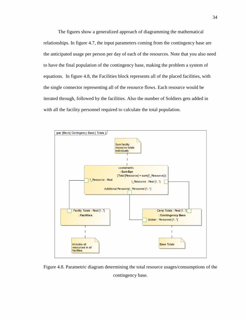
The figures show a generalized approach of diagramming the mathematical
relationships. In figure 4.7, the input parameters coming from the contingency base are
the anticipated usage per person per day of each of the resources. Note that you also need
to have the final population of the contingency base, making the problem a system of
equations. In figure 4.8, the Facilities block represents all of the placed facilities, with
the single connector representing all of the resource flows. Each resource would be
iterated through, followed by the facilities. Also the number of Soldiers gets added in
with all the facility personnel required to calculate the total population.
Figure 4.8. Parametric diagram determining the total resource usages/consumptions of the
contingency base.

35
4.4. MBSE MODEL ANALYSIS
SysML models can also be exported and represented as data in an Extensible
Markup Language (XML) format. XML is a user-defined text format for exchanging data
that is both machine-readable and easily understood by a person [OMG MBSE]. It has a
hierarchical structure using elements and tags defined by the user, or in this case, the
organizational standard. Since there is no standard as to how the information can be
organized within the file, a schema is created and made available so that other
applications know how to read the structure.
An external tool developed for this project takes the model data and populates a
user interface (Figure 4.9). In the user interface, contingency base planners can make
alterations to the usages of the abstract facilities or the estimate high level usages of the
base, and see the totals reflected instantaneously. The planner can also turn facilities on
or off which would translate to whether they would be used or not on the base. When
everything resembles what the planner was anticipating, the new values overwrite the
values originally in the XML. When the model is exported back into the SysML tool,
those changes are reflected in all of the objects modified by the planner. This operation
can be performed as many times as necessary to lay out a contingency base design.
Each model that is generated can be saved as its own model or written out into a
report. The models can then be compared in a trade study to determine which design fits
the mission and objective the best. There might be a desire to reduce fuel or water use on
a base. The dining facility block is altered to be one that uses less potable water, but
produces more solid waste. The solid waste production increase would yield an increase
in fuel use from having to transport more waste. This tradeoff may not be an acceptable

36
alternative, or it could fall within performance parameters of the mission. Due to the way
the facility blocks were created, this can easily be done for any facility and see the
outcome to the overall contingency base system. Some facilities may also be completely
removed from the base, or new ones added into the base. The outcome of this step details
a contingency base that performs the given mission with the least amount of resource
consumption and production (if resource usage is a key performance parameter for the
design).
Figure 4.9. Screen capture of the GUI tool that utilizes model data.
As part of an exercise in generating alternative bases, four cases were generated to
compare the total resources loads of the contingency base. The cases are as follows:
Case 1: All facilities and initial values are set to default for a 500 operational
Soldier contingency base.
Case 2: Starting from the defaults in case 1, it was determined that the average
power consumed per person per day should be 1.5 times the default because of some new
equipment being introduced.

37
Case 3: Starting from the defaults in case 1, it was determined that dining
facilities would be Meals Ready to Eat (MRE)-only facilities. Power, fuel, potable water,
gray water, black water, and maintenance have been set to zero in the dining facility
block.
Case 4: Starting from the defaults in case 1, it was determined that some of the
non-essential facilities should be removed. The post office, education center, religious
services, and tailoring have been removed.
Table 4.1. Total resources required or produced given the alternative cases.
Case 1 Case 2 Case 3 Case 4
Power Consumed (kw) 2928.28 4416.33 2341.1 2562.39
Fuel Consumed (gal) 5215.85 7239.62 4448.98 4888.49
Potable Water (gal) 38236 38444.15 31854.14 34863.25
Bottle Water (gal) 2590.58 2604.68 2497.17 2655.14
Storage Area (SqFt) 4862.88 4889.36 4687.55 4307.94
Personnel 426 431 392 368
Gray Water (gal) 26645.94 26791 24144.11 24224.35
Black Water (gal) 7942.9 7986.14 7050.06 7223.25
Solid Waste (lbm) 15225.66 15308.54 14676.7 12201.92
Food (lbm) 7401.65 7441.94 7134.78 6937.1
Area (SqFt) 119895.8 120548.5 115573 108154.6
Maintenance (hrs) 346.95 348.84 271.57 312.17
Total Population 926 931 892 868
The results, listed in table 4.1 show how changes to the contingency base affect
the totals for the resources. Some of the changes might not be expected, like an increase
in the population in case 2. This is caused because an increase in power demand requires
more fuel and possibly more generators. More fuel requires more personnel to handle the
fuel, and more generators mean more maintenance hours to perform and personnel to

38
look after them. The more personnel increase resource consumption and production in all
resource flows. The results show third order effects not necessarily anticipated. For case
3 and 4, there are reduced resources that need handling, which reduces the number of
personnel required on base. In case 4, bottled water actually increases slightly whereas
many other resources show decreases.
4.5. MBSE CONCLUSIONS
It should be noted that finding the optimal facility layout and determining the
optimal logistics pattern was beyond the scope of this research. Arranging facilities in a
way that increases its performance is a topic that should be pursued, and the facility
layout problem looks to be a promising approach [Drira et al, 2007]. Issues that would
arise in this process are the dynamic nature of contingency bases and the use of ad-hoc
systems that cannot necessarily be anticipated. Dynamic layout problem solutions could
apply, but rely on knowledge of future conditions [Drira et al, 2007]. There has been
some initial research in facility layout optimization, [Robertson et al, 2001] and [Ezell et
al, 2001], with limited results. In [Robertson et al, 2001], they encountered issues in a
constraint on the number of components.
The validation and verification would accurately be achieved when a designed
base is built and put into operation. However, through the use of vetted information on
contingency base parameters and engineering design tools it is possible to perform much
of the validation as the system is being refined. This requires subject matter experts to
analyze the models developed or walked through the process of creating such models,
and giving their verbal validation that the modeled base is approximately accurate. For
more proper validation and verification, a detailed simulation tool that utilizes Soldier

39
schedules, use curves of facilities, and engineering principles is required. At this point,
this framework gives a high level analysis of the contingency base system. Being able to
receive preliminary analysis results as the base is developing will speed the design
process and improve the final contingency base designs produced. In addition, a
repository can be updated with more accurate representations of resource usages from
information in previous designs and constructed designs as well as additional information
provided from the field. This feedback loop will enhance the model to give more accurate
representations of the modeled bases.
The results of this work highlight the interrelationships between elements of an
operational contingency base and the coupling that occurs between these elements. Using
a SysML tool, diagrams are used to show the sources and sinks of utilities. To manage
the inherent complexity in these systems, much of the effort must be put forth early to
develop appropriate requirements that will produce a sustainable and adaptable system.
The use of a SysML tool to visualize the relationships, describe the processes, and refine
the requirements provides a framework for base camps that captures subject matter expert
input to make it available for new contingency base designers.
The MBSE approach described here allows for rapid design and analysis for a
high level architecture of a contingency base. In addition, it can serve as a training tool to
prepare future designers. Presenting users with the design options and showing how they
interact helps with system understanding, aiding comprehension and learning. For
example, many parts of contingency base operations were not known when the project
began, but as information was gathered it was possible to create a full and accurate
contingency base model. By working with subject matter experts from the field and using

40
the diagramming tools provided with SysML tools, information related to the design of
contingency bases was shared much faster and more completely than previous attempts
without the tool.
Using this framework designs are put together for the different parts of a base and
then validated by subject experts for accuracy. Constructing the model as a team helped
the project members better understand contingency bases, as many of those involved in
the model development were not familiar with contingency bases and how they were
operated. The diagrams create useful presentation material that can be reviewed or
discussed with people involved in the project. Many of these diagrams came from
brainstorming on a white board first. The diagrams, specifically the ones highlighting
interconnections, help determine secondary and tertiary effects. For example, an increase
in potable water to a facility will increase the power the pump needs to move the water,
which increases the amount of fuel to provide the extra power, which increases the
number of personnel needed to handle the extra fuel. The increase in personnel will
trickle through all other facilities because they are on the base using resources. Existing
bases could be analyzed if any design changes are required due to a proposed change in
mission or soldier population using this method. This could lead to monetary savings and
having fewer soldiers in harm’s way because fewer resupply convoys are necessary.
The development of this contingency base design tool illustrates a capability in
MBSE that is not normally highlighted: the ability to visualize information to solicit
information from non-engineer subject matter experts. By graphically showing the
conditions and layout of the proposed contingency base, DoD personnel not trained in
modeling and simulation were able to interact with the engineering designs and identify

41
gaps in the proposed architecture. This can prove a valuable tool in projects requiring
requirement solicitation from stakeholders not familiar with system design and
integration.
Creating a domain-specific profile for contingency bases would also be beneficial
because it allows for more customization and would be essential for creating a library of
design choices. This also makes it possible to develop software tools for automatically
creating contingency base designs based on provided requirements. Contingency base
designs can then be easily and quickly configured in different sizes and using different
facilities. These designs would serve as a template that a planner could then refine to the
specific mission using a set of external analysis tools. The templates could also be used as
starting points for future mission designs to accelerate development further.
By modeling the system in an abstract way, analysis can be performed before
designs or components are finalized. Heuristics and historical averages about resource
consumption and/or production play a more important role in the planning phase as
opposed to the exact specifications of a facility. Getting the exact specifications can be
unreliable as actual components used in operation can be unpredictable. Resource
consumptions and productions can be easily modified to run the analysis for different
configurations. Also, having the system as a computer model allows it to easily be
exported and run through external tools and simulations to see how it performs in
different scenarios, or the mathematical model solved to determine resource
requirements. Then the result can be imported back into the model so everything can be
connected and traceable. The model and analysis results are validated by experts familiar
with contingency base planning and operations.
42
One issue currently being addressed by the military is retention of the knowledge
of contingency base planning. During the course of this project, an information gap was
identified pertaining to planning and setup procedures and utility usages by facility types.
New planners have to go through numerous learning experiences rather than accessing
institutional knowledge already developed by senior planners. Workshops have been
conducted to get a knowledge management system in place so information can grow and
evolve instead of remain static. The ArmyBaseCamp/JFOB.net knowledge management
system contains information from all branches of the military on contingency basing
through the use of briefings, interviews, documents, books, best practices, and policies
[Trainor et al, 2008]. With the knowledge management system and the ability to store
system models in a repository, collaboration among different planners is now possible.
New planners start off with base templates, and have rationales as to how a base was
setup and laid out.
4.6. APPLICATION TO STUDENT DESIGN TEAM
University design teams typically suffer from problems unique to academia
including high personnel turnover, a limited time commitment due to classes, lack of
experience and knowledge, and keeping consistency across all subsystems. The issue,
like in base camp planning, is with knowledge management and educating inexperienced
designers so they can begin contributing. Here we will apply the methods used for base
camps to the M-SAT Design Team. The method typically used on projects of this nature
to help with this issue is a document tree that includes documentation of all designs, tests,
procedures, code, etc. Each document includes a revision section in order to track
changes. Occasionally, errors are found in the documents. Design changes may be

43
overlooked, or understanding of design choices may be lost with new members. The
model-based approach is a possible method to also help address the consistency and
knowledge problems, and better verify requirements with simulation analysis.
The main focus for modeling the base camp was on the blocks representing the
facilities. In the case of the satellite project, all aspects of MBSE and SysML are taken
into account and modeled. This includes requirements, structure, behaviors, parametric
analysis, and traceability. Particularly with the parametric analysis, there is some overlap
with the base camp project with using the XMI generated file in an analysis application.
The information about the M-SAT Design is relevant only for when I was active
on the team while participating in the Nanosat 7 program. The Nanosat 7 program is a
joint program between the Air Force Research Laboratory’s Space Vehicles Directorate,
the Air Force Office of Scientific Research and the American Institute of Aeronautics and
Astronautics. The competition lasts two years and challenges student design teams to
design and fabricate a prototype satellite. The winning team will get the chance to launch
their satellite as a secondary payload on a launch vehicle into orbit about the Earth.
4.6.1. Requirements. The primary objective of the M-SAT team is to fly two
satellites that will operate in close proximity. One satellite will act as a Resident Space
Object (RSO), and the other as an Inspector satellite. The Inspector satellite will attempt
to calculate the Ballistic Coefficient of the RSO. The secondary objective is to
circumnavigate the RSO and create a 3D model from images to ascertain the RSO’s
capabilities. Much of the design is heritage from previous competitions to reduce the
design time required, helping the satellite be completed on time. Each design choice has

44
been consistently researched through trade studies to ensure they still meet the
requirements.
First, requirements are put into the model. These were already in a worksheet
format that includes id#, requirement, source, verification and testing documentation.
One area that was discovered missing in the document is a rationale for the requirements.
The benefit of adding the rationales is added details about where the requirement is
developed from aside from the source requirement. For example, many of the structures
requirements come from University Nanosat Program requirements provided in the
User’s Guide. The rationale points the reader to a specific section of the User’s Guide
with the requirement.
In the model, it is also easy to separate and display information for anyone who
wants extra information about a particular area. A diagram is created that shows all
system level requirements of the Inspector satellite and which mission requirement they
are derived from. If someone wants more information about system requirement 2, which
relates to operational period in orbit, they can double click on that requirement to open
the S1-2 requirement diagram. (Provided the modeler creates that particular diagram and
links it). The diagram (Figure 4.10) displays the rationale, ‘satisfied by,’ and ‘verified by’
information. Depending on the depth of the model, either the ‘satisfied by’ or ‘verified
by’ could have linked diagrams that contain even more information. The ‘verified by’ test
case could include information obtained from an analysis tool, like a power budget.

45
Figure 4.10. Transition from documented requirements to model requirements.
4.6.2. Physical System. Like the contingency base, the physical system is
modeled going from a level of abstraction to details. First, a block definition diagram is
created with the different subsystems on each satellite (Figure 4.11).

46
Figure 4.11. Block diagram of satellite subsystems.
Each subsystem block opens up to another block definition diagram containing
the hardware for the particular subsystem (Figure 4.12a). Some are more detailed than
others, as not all designs have been finalized. However, the lack of design information
was occasionally due to a lack of documentation. Documents might contain design
choices but lack specifications about the hardware. One issue with an MBSE approach
noticed early on was determining what should be a block and what should be a part. For
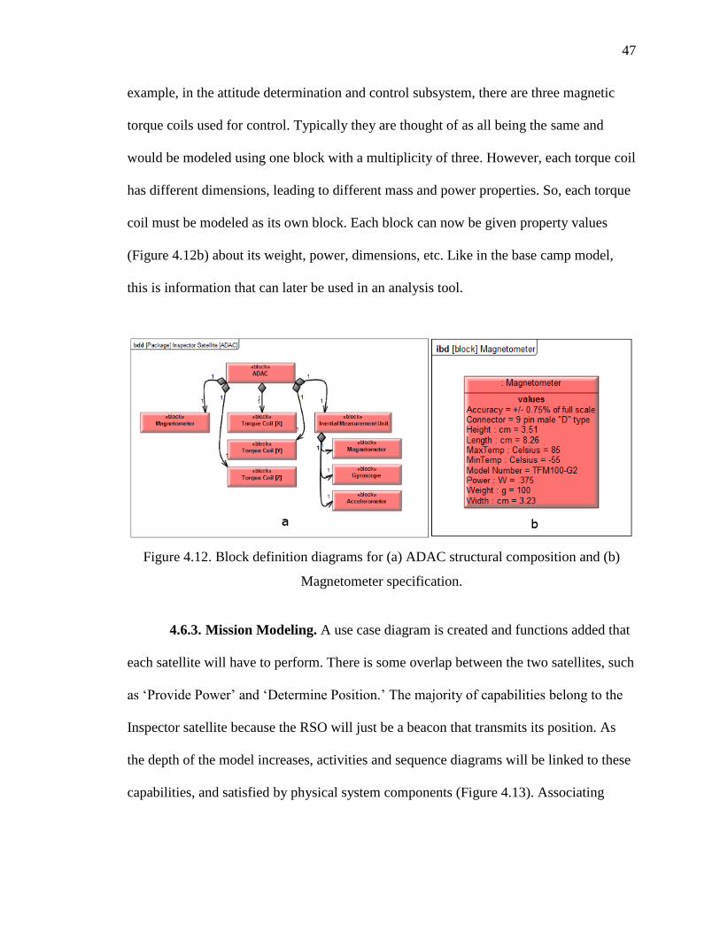
47
example, in the attitude determination and control subsystem, there are three magnetic
torque coils used for control. Typically they are thought of as all being the same and
would be modeled using one block with a multiplicity of three. However, each torque coil
has different dimensions, leading to different mass and power properties. So, each torque
coil must be modeled as its own block. Each block can now be given property values
(Figure 4.12b) about its weight, power, dimensions, etc. Like in the base camp model,
this is information that can later be used in an analysis tool.
Figure 4.12. Block definition diagrams for (a) ADAC structural composition and (b)
Magnetometer specification.
4.6.3. Mission Modeling. A use case diagram is created and functions added that
each satellite will have to perform. There is some overlap between the two satellites, such
as ‘Provide Power’ and ‘Determine Position.’ The majority of capabilities belong to the
Inspector satellite because the RSO will just be a beacon that transmits its position. As
the depth of the model increases, activities and sequence diagrams will be linked to these
capabilities, and satisfied by physical system components (Figure 4.13). Associating

48
physical components is beneficial to knowing which components will be running while
performing a specified task.
Figure 4.13. Use case diagram showing the use case linked with an activity diagram.
The states, or operational modes, of the system are based on the previous
competition’s operational modes. They are then modified, deleted, or added to as
required to fulfill the new mission. The first step was to create a state diagram that
included all states, and why, or when, the system will move from one state to another
(Figure 4.14a). Each state is then linked to an activity diagram that walks through the
general activities performed during that state (Figure 4.14b). Eventually, many of these
activities will link to diagrams that contain more activities required to perform that higher
level activity. This is already a defined process within systems engineering.

49
Figure 4.14. Behavioral analysis showing (left) Operational Modes of the satellite and
(right) Initialization Mode activities.
The benefit of using a model in this project is providing an easier method to walk
through the lifecycle of the system. Each of the high level activities terminates at the start
of another state, and by double clicking the termination point the next state’s activity
diagram opens. A person looking through the model would be able to navigate through
the functional flow like they would navigate through a website. Another benefit is that
processes are beginning to be determined for each state. Now the state will have a set of
activities associated to it, and activities associated to hardware. So, a list of hardware
running during each state could be generated for analysis. Depending on the work that is
put into the details of the model, this could help produce either a rough calculation for
power consumption or an accurate model of power consumption.

50
4.6.4. Analysis. Some of the common analysis performed on a satellite early on is
the power budget, mass budget, and data budget. These are performed to know how much
power is being consumed, the mass of the satellite, and memory that needs to be stored.
These all have constraints, or requirements from the customer in the case of mass.
The same process used for the army base camp can be applied to the satellite
project. A domain-specific profile for satellites may also need to be created. The model
could be exported out in the XML format, and the hardware and state information
extracted. The information could then be used in a totals analysis tool based off the base
camp one (Figure 4.15).
The interface would again be separated in sections for mission mode, totals,
component selection, and component details. The mission mode could contain the
selection of modes. When a state is selected, components that are active during the state
would be automatically selected. Totals for that state would then be calculated and
displayed. There would also be the option to turn on/off components. This analysis tool
would work well for power mostly because mass will not change due to a component
being active or inactive. Additional types of analysis tools could be developed as well for
each type of analysis that needs to be performed. The results could then be imported back
into the model as those test cases that verify requirements.

51
Figure 4.15. Theoretical user interface for satellite totals analysis.

52
5. AGENT BASED MODEL
Agent-based modeling is an object oriented approach to simulate independent
behaviors with interactions. The common reason for using Agent-Based Modeling
(ABM) is its ability to explicitly model complex behavior originating from individual
entity’s actions and interaction with other entities [Siebers et. al., 2010]. When the
system’s environment is dynamic and there is a need to be able to adapt to changing
requirements and events, ABM is a common approach to model these conditions. This is
even more important when real-time responses are desired, such as the desired
improvements for DCAM. Each component type has wide ranging characteristics from
other types, and each component within each type differs in their attributes. Most
operations models, like discrete event simulations or system dynamics, take the approach
of stating what should be done for the system rather than how the system operates in
realistic conditions [Siebers et. al., 2010]. Since ABM is object-oriented, it is easily
extensible like the MBSE and DCAM methods.
There is research already conducted that is relevant to contingency basing. There
were many research topics at the 1999 Workshop on Agent Simulation that dealt with the
recently deregulated U.S. electrical industry. One paper used adaptive agents to model
the industry as a commodity and exchange model [Sheble, 1999]. On the base, some
facilities have a higher priority, or bidding power. If the supply of power were to fall
below the demand, then the adaptable agent would be able to figure out how to supply the
power based on bidding power, or priority. Another modeled the consumption behaviors
of customers with agents [Tsoukalas and Uluyol, 1999]. Demands could be predicted,

53
and electrical components could implement decision making that handles that anticipates
the predictable behavior or offer contingency plans for unpredictable behavior.
Logistical planning also includes other resources like water and waste. Existing
simulations of supply chains have narrow applications [Tan et. al., 2009]. Tan et al found
that applying agent-based framework could improve extensibility of a supply chain
model. They also found the emergent behavior of complex supply chains difficult to
understand, which is where agent-based modeling excels. Jiaxiang developed a multi-
agent system framework to improve emergency response in large catastrophic events
[Jiaxiang and Lindu, 2008]. The logistics management system is able to search for and
procure emergency material for the response to the catastrophic event. Contingency bases
have emergency situations that require additional logistics; however, this would be
outside the scope of the contingency base and more along the lines of the theater level.
Supply chain management is also an area with agent-based modeling use. There is the
ability to dynamic reconfigure the supply chain system [Zhang and Tao, 2008]. They
made the model reconfigurable to respond to changing requirements and operating
environments. As stated earlier, contingency bases have a very dynamic operating
environment. They found dynamic reconfiguration to benefit robustness, flexibility, and
agility of the supply chain. In emergency situations on the base, it would be beneficial to
be able to reconfigure the supply chain. Agent-based modeling has also been applied to
abnormal, or disruptive, situation management in the area of industrial networks and
supply chains [Behdani et. al., 2011]. Again, there are plenty of opportunities for a
contingency base to enter an abnormal operating state due to a disruption from external
and internal elements.

54
5.1. AGENT-BASED MODELING BACKGROUND
The agent element has roots in many diverse research disciplines including
sociology, biology, distributed systems, and other [Yilmaz, 2009]. The ability to adapt is
one of the prominent characteristics are an agent. The autonomy and use of multiple
agents has been a popular area of expansion [Jennings et. al., 1998], and still continues to
mature with many applications being developed and deployed [PAAMS, 2013].
Despite the proliferation of agent-based modeling in numerous and varied
disciplines, there is no formal definition of an agent. The common theme though is that
an agent is an independent element (Figure 5.1). The behavior aspect of the agent is
where the definition varies the most. Since the basis of this research is in the Systems
Engineering domain, the working definition will follow a combination of definitions
provided in Agent-Directed Simulation and Systems Engineering [Yilmaz, 2009] and by
Macal and North [Macal, 2006]. The definition, like most, is broken into components
which include:
Identifiable. The agent is an individual with attributes and behaviors. There may be
many of one type of agent that share attributes and behaviors, but it will be made up
of individuals with separate values for the attributes.
Situational Awareness. The agent can see its environment and act within or on the
environment. The environment can be other agents, dynamic object, or passive
objects. The agent can interact with all other agents or objects, or specific agents or
objects. There is a social aspect of dialogue between agents.
Goal-Oriented. The agent has a goal, or purpose. It may be to just continue to
operate, and not necessarily optimize an objective.

55
Autonomous. The agent must be able to operate and make decision with no human
interaction. The agent has a behavior and will act according to that behavior.
Adaptable. The agent should be able to learn and change its behavior over time, based
on previous experience due to changes in environment, constraints, or requirements
Figure 5.1. Properties of agents [Macal, 2006].
Agent-based modeling and object-oriented programming have many similarities.
Object and agents are encapsulated entities, are able to perform actions, and can
communicate [Jennings, 1998]. There are a couple of differences, with objects being
thought of as a basis for an agent. First, the agent has control over what actions it
performs. Another agent can only request an action be performed. An object has no
choice. If another object calls for an action to happen, it happens. The slogan goes:
“Objects do it for free; agents do it for money” [Jennings et. al., 1998]. Second, agents
have flexibility in their autonomous behavior. Object-oriented programming does not
include these types of behavior customarily.

56
An agent-based model can be made up of one or more agents. Typically, there is
more than one agent in the environment [Yilmaz, 2009]. For multi-agent systems, a
single agent is unable to solve the problem on its own, usually due to incomplete
information or capability. When there are multiple types of agents, the agent space is said
to be heterogeneous. Even in homogenous spaces, behaviors may differentiate based on
agents’ states and initialization parameters. Agents have the ability to cooperate or
compete with other agents, as well as, form and dissolve networks. One of the prominent
benefits of agent-based modeling is their ability to change their network of agents with
whom they interact.
The agent space environment, or situated environment [Yilmaz, 2009], can be
characterized certain categories:
Deterministic or Stochastic. In a deterministic state there is only a first order
effect from an action. In the stochastic state, chain reaction event are possible
from a single originating action. This would be like the secondary and tertiary
effects that were observed in the MBSE method.
Episodic or Sequential. With episodic, the action and effect is limited to the
current step. Sequential means actions can have effects on future steps too.
Static or Dynamic. In a dynamic environment, environment attributes and objects
can change. This could be as simple as an object moving through the
environment.
Discrete or Continuous. Discrete is separate and distinct, while continuous uses a
function based on a step function like time.

57
Agent-based modeling has many application areas, but is not always necessary.
Macal has noted where agents excel over other simulation methods, like discrete event or
system dynamics, multiple times, [Macal and North, 2006] and [Siebers et. al., 2010]:
A desire for agent with a natural representation
Decisions and behaviors defined discretely
When the behaviors need to be flexible and able to adapt
When agents learn and engage in strategic behavior by anticipating other’s
reactions
When the problem has dynamic relationships, where agents form and dissolve
relationships
When there is a spatial component to agent behavior
When self-organization is important, through agent cooperation or collusion
When the future is unpredictable based on past information
When process architecture is an output and not an input
When extensibility is important
Since agent-based modeling has roots in object-oriented programming, it can
utilize the Unified Modeling Language (UML) as well as the Systems Modeling
Language (SysML) because SysML contains all capabilities associated with UML. There
is varying research on agent-based modeling and SysML, from conceptual design and
representation [Sha, 2011] to executing agent-based UML diagrams in [Ehrler and
Cranefield, 2004] and [Da Silva et. al., 2004].
Previous research has shown that contingency bases can be represented through
SysML diagrams. Those diagrams were also utilized in creating an executable tool. That

58
previous research can expand to include agent representations. Systems are already
represented as objects like the research here. The addition of object behaviors, like agents
incorporate, would be represented through state diagrams, sequence diagrams, and
parametric diagrams. Automatic code generation allows the diagrams to be executable.
Utilizing similar model libraries in the MBSE method, behaviors can be swapped in and
out for agents. The executable agents now have high adaptability properties. Also, as was
seen with the MBSE, the diagrams help with system understanding. This will help
include experts in tactics and procedures in the designing and verification processes.

59
6. AGENT SIMULATION
The agent-based model is made up of four different agent types: Soldier group
agents, component agents, system agents, and generator agents. Each of these agents can
be instantiated any number of times. The agents are used to capture the individualized
behaviors. There are differences in how Soldier groups behave, especially between
contractors and Soldiers. On the larger camps, nearly half of the population could consist
of contractors. Facilities also operate differently. In Billets, there are outlets for personal
electronics. Contrarily, the Medical facility likely has no personal electronic use. In
emergencies, Billeting is more likely to cut down on power usage where Medical would
not be able.
6.1. AGENT INPUTS
Each agent type discussed previously will require and use different inputs as
follows:
Soldier Group Agents
o Number of persons. Each Soldier Group Agent will have a given number
of persons that belong to the group. An example of a Soldier Group would
be a specific platoon. That platoon would be made up of a number of
Soldiers.
o Type. Soldier Group Agents could be made up of Soldiers or contractors.
This distinction will affect the way the agents behave. There could even be
a distinction between Soldier types. A Special Forces group will not
behave exactly the same as an infantry group or engineering group.
60
o Operational schedule. Every Soldier Group will have a schedule to
determine when the group is on duty or off duty. When off duty, the
persons reside in non-operations areas like billeting or recreation facilities.
When on duty, they could be off base or in operations areas.
o Facilities to use. Each Soldier Group will be assigned certain facilities,
like billeting tents that are specifically used by that group. They may be
assigned latrines and showers given proximity to their billeting tents, but
could also use any latrine or shower on the base.
o Components. Within each facility assigned to the Soldier Group are
components of which state they can directly affect. This would be personal
electronics in the billeting.
Facility Agents
o Components. Each Facility Agent knows the types and number of
components within its system boundaries.
o Generators. Each Facility Agent knows which generator it is directly
connected to if that is the case. In electrical grid cases, it is not connected
to any single generator. However, electrical grids are still not implemented
on contingency bases so there is a need to have the facility connected to a
generator.
Component Agents
o Operational profiles. This will not be applicable to all Component Agents.
Operational profiles designate times the agents are running, regardless of
any other influence. This would be kitchen appliances using resources

61
around typical breakfast, lunch, and dinner times. Another profile could be
ON 24 hours, like components in the TOC.
Generator Agents
o Power Capacity. The maximum allowable capacity.
o Power Demand. The Generator Agents will track total power demand that
is requested from attached Facility Agents and their Component Agents.
6.2. SIMULATION SPECIFICS
Each simulation is based on a one-minute time step. The simulations are run
multiple times to simulate multiple days as required. For each time step, the Soldier
group agents first determine if they are on or off base. If they are on base and off duty,
then they determine what component, or components, they use. Next, each system agent
is run. Each system agent will go through each of their components. For each component
agent, they update their on or off state based on their operational profile, if they have one.
The on or off state is also changed by the Soldier group agent. If the component agent is
in the ‘ON’ state, then it requests power from the generator agent, as specified by the
system agent. If the state is ‘OFF’, then nothing happens.
Finally, each generator agent is run, first checking to see if it is operational. For
example, there is the possibility that it failed due to mechanical issues. If it is operational,
then it checks if it can produce enough power to supply all of the requests from the
component agents. If there is enough supply, then all component agents receive their
requested power. If there is not enough supply, then no component agents will receive
their requested power, as the generator agent was overloaded. The generator agent saves
a history of its power production and it efficiency for each time step. The efficiency helps

62
to determine the cumulative daily fuel usage. The fuel usage rates are based on an
“Approximate Diesel Fuel Consumption Chart” from Diesel Service & Supply [Diesel,
2014]. The chart splits the fuel rates by generator size and load percentage at a rate of
gallons per hour (Table 6.1). To develop the values in table 6.1 from this work, it was
necessary to convert the consumption rates to gallons per minute. Then, trend lines were
calculated for each generator size. The trend was linear and generated a continuous
function to calculate the fuel consumption rate based on the efficiency. Finally, two trend
lines were calculated from all of the generator sizes. These trend lines, also linear in
nature, are used to calculate the slope and intercept of the consumption equations. Now
fuel consumption has a continuous function given a generator capacity and efficiency.
Table 6.1. Approximate Diesel Fuel Consumption Chart (provided by Diesel Service and
Supply)

63
6.3. CREATING A BASELINE MODEL
A basic system is modeled to create a baseline for comparative purposes. There
are 3 Soldier groups, 3 100 kW generators, and 3 billeting tents with lights and an
environmental control unit (ECU), see Figure 6.1. The power demands at this point are
notional. Each component agent is modeled in such a way that the value could be
adjusted to any value the user desires. The numbers were not as important at this point as
was the behavior of the model. The ECU in each billeting tent was given an operational
profile where it would consume 30 kW from 0900 to 1800. The lights operational state is
determined by the operational schedule of the Soldier groups. When the Soldier groups
went off duty, they turn the lights on. At this point, lights just stay on. Additional detail
could be incorporated to turn lights off at night when Soldier groups are asleep. For the
simulation, a single day is simulated at a one-minute time step. Each generator’s
cumulative fuel usage per day is calculated, and the camp total for daily fuel usage is the
basis for all comparative analysis.
The results of the run are shown in Figures 6.2, 6.3, and 6.4. The first figure
shows the efficiency of ‘Generator 1’ producing power for ‘Billeting 1’ under the
operational profile of ‘Platoon A’. The second and third figures follow the same pattern.
The generator agent displays the efficiency. The system agent displays the total power
usage off all component agents within that system. The Soldier group agent displays their
operational status, with ‘0’ being on duty and ‘1’ being off duty. The individual generator
fuel usage and total camp fuel usage of this initial configuration is shown in Table 6.2.

64
Figure 6.1. Architecture of the baseline agent model.
Figure 6.2. Generator 1 power profile with connected system and soldier group.

65
Figure 6.3. Generator 2 power profile with connected system and soldier group.
Figure 6.4. Generator 3 power profile with connected system and soldier group.

66
Table 6.2. Initial Configuration Daily Fuel Usage.
Fuel Usage (gallons)
Generator 1 96.19
Generator 2 103.9
Generator 3 96.19
Camp 296.28
6.4. ADAPTABLE ARCHITECTURE
The simulation was developed so that it has the ability to change the architecture
of the entire system. The generators contain the ability to change which systems are
connected to them in order to find a more efficient model. The method employed shares
characteristics of reinforcement learning, specifically a variation of Q-learning. Each
generator will try all possible solutions and score them based on the generator’s average
efficiency. If a generator is overloaded at any point during the simulation, then the score
for the solution will be given a ‘-2’ to specify that it is a configuration that would not be
able to function. The actions that can be taken by the generators are based on
evolutionary algorithms. They are swap, give, or take. The generators will go through the
actions one at a time. In swap, one generator will swap a single connected system with
another generator. If there are no swaps that would give the generator a new
configuration, then it moves on to the take action. In take, the current generator takes one
or more connected systems from another generator. Again, if no possibilities yield a new
solution for either the current generator or the generator being taken from, then the
generator moves onto the give action. In give, the current generator will give another
generator one or more of its connected systems. Finally, if no solutions are found for the
generator, then that generator has no more possible solutions. When all generators reach

67
the point where no more new solutions are possible, then the search stops. During each of
the actions, if an action takes place, then both involved generators will switch to a state
where they can no longer be looked at for swapping, taking, or giving to other generators.
The system is told to adapt, and find a more optimized configuration. This is just
one of the possible applications of the adaptable architecture. The computed score table is
shown in Table 6.3. Each generator has a priority. When all possible solutions are found
and scored, the highest priority generator goes first and chooses its best scoring
configuration. The systems chosen are removed from a list of available systems. The next
highest priority generator goes through all of the solutions that only contain the
remaining available systems, and chooses the highest scoring solution of that subset. This
continues until no more available systems remain.
Table 6.3. Solution scoring table for each possible generator configuration
Billeting
[] [1] [2] [3] [1, 2] [1, 3] [2, 3] [1, 2, 3]
Generators 1 0 0.2 0.19 0.2 0.39 0.4 0.39 -2
2 0 0.2 0.19 0.2 0.39 0.4 0.39 -2
3 0 0.2 0.19 0.2 0.39 0.4 0.39 -2
The reconfigured system has ‘Billeting 1’ and ‘Billeting 3’ connected to
‘Generator 1’, and ‘Billeting 2’ still connected to ‘Generator 2’. There is no system using
Generator 3 in the final configuration. The detailed power-related graphs of ‘Generator 1’
with the new configuration are shown in Figure 6.5. Now, there are two Soldier group
agents off duty during the middle hours of the day. Since they both have the same
schedule, the power required to be produced by ‘Generator 1’ and its resulting efficiency

68
is doubled when loads are operating. The efficiency reaches near 100%, where before it
barely hit 50%. ‘Generator 2’ still interacts with the same system agent as the baseline
run, and produces the same results shown in figure 6.3. Since ‘Generator 3’ has no
system agents using it, the power produced is a constant at zero. Therefore the graph was
not included. The individual generator fuel usages and total camp fuel usage for the new
configuration is shown in Table 6.4.
Figure 6.5. Generator 4 power profile with new connected systems and soldier group.
Table 6.4. New Configuration Daily Fuel Usage.
Fuel Usage (gallons)
Generator 1 172.22
Generator 2 103.9
Generator 3 0
Camp 276.12

69
For the system considered here, there is a savings of about 20 gallons of fuel per
day. Using a conservative estimate of about $20 for a gallon of fuel and its transportation
to the camp, then this yields a savings of $400 per day. After 60 days, it’s about 1200
gallons and $24,000 savings. After 180 days, it’s about 3600 gallons and $72,600
savings. This does not include the reduced risk to personnel in possibly reducing the
number of supply convoys.
Another application area for this adaptable architecture is for unsteady state
analysis. Occasionally on camps there is a surge of Soldiers and more billeting tents must
be placed. The adaptable architecture can take the additional systems and connect them to
generators that would again optimize fuel usage.
For a specific example, we take the baseline architecture and add 3 more billeting
tents. Each billeting tent is identical to those in the baseline and each comes with its own
100 kW generator. The main difference is that the surge troops are off duty all day. The
unoptimized and resulting optimized surge scenario results are shown in Table 6.5. This
architecture has each generator supplying power to one billeting tent. After optimization,
the architecture has ‘Generator 1’ supplying power for ‘Billeting 4’ and ‘Billeting 6’,
‘Generator 2’ supplying for ‘Billeting 1’ and ‘Billeting 5’, ‘Generator 3’ supplying for
‘Billeting 2’ and ‘Billeting 3’, and the rest of the three generators not being used. The
results show similar fuel savings compared to the first optimization problem. After 180
days, 8838 gallons of fuel has been saved which equates to $176,760. This analysis could
be run before the surge and planners would know how many extra generators would be
required.
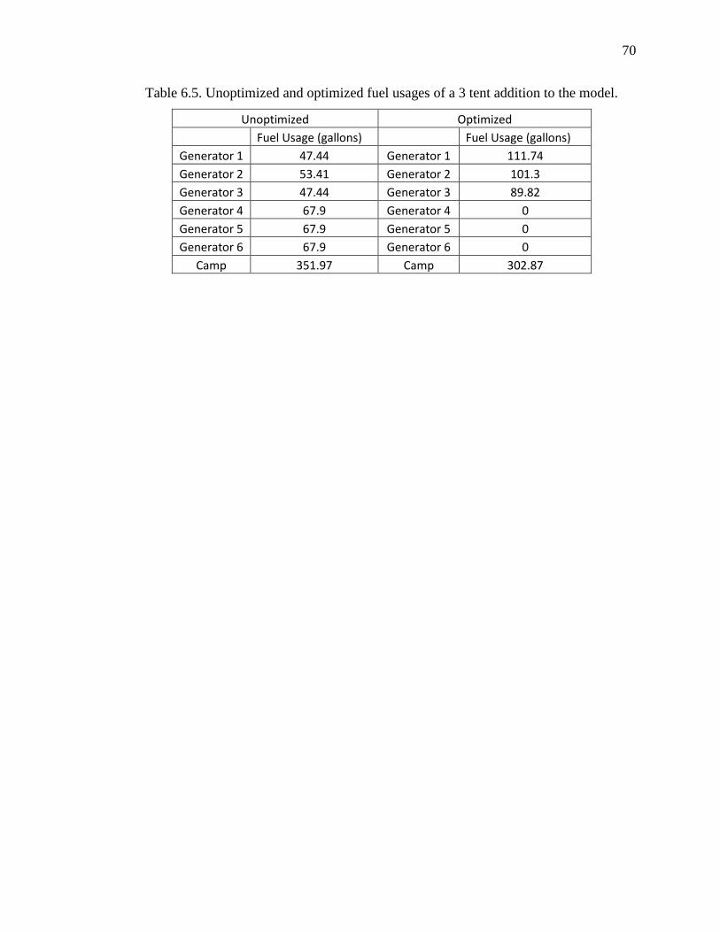
70
Table 6.5. Unoptimized and optimized fuel usages of a 3 tent addition to the model.
Unoptimized Optimized
Fuel Usage (gallons) Fuel Usage (gallons)
Generator 1 47.44 Generator 1 111.74
Generator 2 53.41 Generator 2 101.3
Generator 3 47.44 Generator 3 89.82
Generator 4 67.9 Generator 4 0
Generator 5 67.9 Generator 5 0
Generator 6 67.9 Generator 6 0
Camp 351.97 Camp 302.87

71
7. EVOLVING AGENTS
Contingency Bases are unpredictable environments. Soldiers’ operational
schedules are not fixed; they will change with hostility conditions outside the camp.
Camp resources are not reliable. Everything is shipped into the camp by either air or
vehicle, which involves extra risks in hostile environments. If a supply chain is attacked,
it could be an extra couple of days before those resources finally arrive. Also, planners
are attempting to improve the quality of life on camps in order to improve Soldier
effectiveness. These improvements to quality of life are typically luxuries that Soldiers
are used to having back home. Luxuries in this age are also typically electronic in nature,
like televisions and gaming systems. If Soldiers have access to these power hungry
electronic devices, power load profiles are far from predictable. Evolving agents will be
able to anticipate, or at least be able to adapt fast enough to provide continuous resource
production, like electrical power.
7.1. EVOLUTIONARY ALGORITHMS
Evolutionary algorithms try to simulate natural evolution processes in computer
code to develop novel and useful solutions to a variety of problems. Evolutionary
algorithms encompass a variety of techniques that share similar attributes: evolution
strategies, evolutionary programming, genetic algorithms (Gas), and genetic
programming (GP) (Parmee, 2001). These methods all develop several solutions at once,
and use current solutions to develop newer solutions. This is similar in nature where
parents pass on a combination of traits to their children.
Evolution strategies (Rechenburg, 1984; Schwefel, 1975) and evolutionary
programming (Fogel, Owens, and Walsh, 1966) are similar but independently developed

72
methods for evolving solutions. Both have solutions that are real valued strings, and new
solutions can be formed by changing one or more values in the string. The difference is
that evolutionary strategies use all solutions to develop new solutions, and evolutionary
programming uses the most fit solutions.
Genetic algorithms (DeJong, 1975; Holland, 1975) use a form of natural selection
to determine which individuals in the population mate. Chromosomes resemble data
arrays normally made up of binary strings that represent real numbers or integers, real
values, or program directions for controlling artificial agents. Like the previous selection
methods, it favors the most fit members but allows for any member to reproduce. The
selected members will undergo operators meant to simulate natural mating phenomenon,
like crossover or mutation. The new solutions will then take over the old solutions.
Genetic programming (Koza, 1992) is different from the previous strategies. It
uses parse trees to store information, with the nodes representing operators, and the
terminals representing constants or variables. Genetic programming is intended to evolve
computer code. Selection and reproduction of the parse trees is similar to the previous
strategies, however are altered slightly to ensure the newly generated solution is
executable. Operands can only be crossed with operands, and terminals can only be
switched with terminals.
Each of these methods has strengths and weaknesses. Evolution strategies and
evolutionary programming have long run times, while crossover is often disruptive in
genetic algorithms and even more so in genetic programming. There is also a problem
with mutation having different impact on a binary string depending on the position at
which the mutation is applied. Evolutionary algorithms can be thought of as using

73
different aspects from these methods to develop a representation of the problem being
studied that can avoid a particular method’s weakness. Using this representation, it is
then possible to choose parameters for the algorithm that properly explore the search
space.
7.1.1. Evolutionary Algorithm Parameters. Different parameters in an
evolutionary algorithm effect the time to convergence and/or the quality of the final
answer. Some parameters effect how the algorithm is initialized and others effect how the
algorithm simulates mating in nature.
Population Size – The population size is the number of members in the population
available to reproduce. The first estimation for an optimal population size was the
Schema Theorem for genetic algorithms introduced by Holland (1975), which estimated a
population size of the order of magnitude of n^3 would ensure that there was a sufficient
representation of possible combinations to solve the problem, where n is the length of the
bit string being used. While binary strings are useful in some applications, many real-
world engineering problems require optimization of real valued functions. One example
of the use of real valued function is the work of Haupt and Haupt (1998; 2000), who
performed experiments varying the population size and mutation rate for real valued
functions. Smaller population sizes and low mutation rates were found to perform best.
Selection Method – Selection method is normally associated with genetic
algorithms and genetic programming. The major schemes are generational algorithm
(DeJong, 1975) or a steady state algorithm (Reynolds, 1992; Syswerda, 1991; Whitley,
1989). Generational algorithm involves all member of the population to mate. Steady
state algorithm selects individuals and mates just the pair selected. Also, a method for

74
selecting individuals needs to be determined. Some of the most popular are fitness
proportionate selection (random selection of parent with higher fitness having a better
chance of selection), rank selection (like fitness proportionate selection, but arranging the
solutions by fitness and then using this “rank” for selection), and tournament selection
(the population is divided into groups, with the most fit members of the group
reproducing) (Parmee, 2001). Closely related to selection method is the algorithm’s
replacement method, which can be absolute (child replaces a population member
regardless of its fitness) or elite (child replaces a population member only if it is more
fit).
Crossover – The crossover operator is how most evolutionary algorithms perform
recombination to generate new solutions. Normally, one or two points are randomly
selected on the parents’ representation strings. A child is produced by copying the data
first from one parent, then switching to the other whenever a crossover point is reached,
called single or multiple point crossover. The chance of crossover occurring is referred to
as the crossover rate.
Mutation – Mutation changes the value at one or more location in the evolving
solution. This makes it possible to introduce an entirely new solution into the population.
Mutations like this also occur naturally in living species. Mutation is normally conducted
by randomly changing one or more values in a newly produced child before its fitness is
evaluated. The chance of mutation occurring is referred to as the mutation rate.
7.2. AGENT INPUTS/OUTPUTS
First, we have to define the inputs and outputs of the agents, see Figure 7.1. The
individual agent inputs will remain the same as those specified in the previous section.

75
We will start with just the generator agent. The generator agent is able to perceive
instantaneous power demand, as well as past power demand. The generator agent can
also tell when Soldier group agents, that use the connected system agents, are off duty.
Knowing when Soldier group agents are off duty is a good predictor that electrical
demands will increase in many different systems. The actions a generator agent can take
start with the simple increasing or decreasing power output. This will scale the generator
output to the level of demand. This saves fuel when compared to running the generator at
full capacity with a lower efficiency. The next level of action includes redistribution of
power. Power demand is passed to other generator agents that have excess capacity. This
will prevent generators from overloading and failing, which could physically damage the
generator or system. The last set of actions is adding or removing a generator from the
overall system. Sometimes, power demand is greater than currently operating generators
can produce. Other times generators are under-utilized, running at low efficiencies and
wasting fuel. Power demands could be consolidated and generators put into a backup
state.
Figure 7.1. Possible inputs and responses of a generator agent.

76
Each agent will have a unique GP – Automata controller by the end of the
training. Then, as long as there were no major changes to the operating environment, that
controller will be sued. Like in many agent-based models and systems models, the
process and observation of any emergent behavior is important. Each agent will store a
history of some of its values like:
Connection network – During steady-state operations, network connections will
remain fairly static and won’t yield many interesting results. However, in a
disruption-state, watching how the network connections adapt into order to
maintain camp effectiveness will be very beneficial. These will introduce new
processes and tactics into operating contingency bases.
Soldier Schedule – Soldier schedules will remain primarily an input to the model
and a main driver to the system. A history of a Soldier Group’s duty schedule will
help in order to view the whole picture and see causation effects. There will also
be instances where schedules change.
Component: Power Usage – Recording of the power usage of a particular
component. This becomes more important with components with a stochastic
usage.
Facility: Power Delivered – The facility agent contains a rolled-up power usage of
all of its contained components. This is also power delivered instead of power
usage. The delivered power will not match usage in cases where generators are
overloaded or operating at a reduced capacity.

77
Generator: Capacity – For generators that are unable to reduce their power output,
then this will be a static line. For generators that can reduce output, this will help
with tracking efficiency, fuel usage and Generator Agent behavior.
Generator: Power Output – The power output is the power used by the connected
facilities. It should be the summation of all the components within the facilities
connected to the specific generator. This will also be an indication of when a
generator is overloaded.
Generator: Efficiency – Generator efficiency is useful in calculating fuel usage.
An average efficiency can be useful in the fitness function for the evolving agent.
Generator: Fuel Usage – The summation of the fuel usage throughout the day will
provide daily fuel consumption for electrical production. This is also useful in a
fitness function.
7.3. EVOLVING AGENTS EXAMPLE
This example presents the implementation of the evolutionary algorithm into the
agent model. It adds evolutionary algorithm functions into the agent behavior,
specifically the generator agent. The objective of the evolutionary algorithm in this case
is to reduce fuel usage on the camp.
For this proof of concept, we focus on simulating the energy usage in the billeting
tents. The architecture of the model is that 4 billeting tents are connected to one (1) 60
kW generator. The billeting tent contains lights, an ECU, and personal electronics which
consume 300 W, 6 kW, and 3 kW, respectively. These components can be represented
within the SysML architecture representing the base camp. The ECU operational profile
is dictated by the information contained within the DCAM model. The lights and now the

78
personal electronics are turned on when Soldier group agents are off duty. The behavior
of the generator agent is not altered in any way from the pre-EA agent in order to produce
a new baseline based on the new architectural configuration. The results returned from
this architecture show that system consumes approximately 47.2 gallons of fuel daily.
A string of real values is used to represent the states of the controller of the
agents. This string includes values for Soldier group agent schedules, the amount a
generator agent’s capacity can decrease in a time step, the number of minutes a generator
agent waits in steady state to reduce the capacity, and the precision for determining if
steady state is occurring. Each Soldier group agent is assigned a random operational
schedule, but to maintain a feasible solution there must be at least one group always on
duty. If the schedules have a situation where no Soldier group agent is on duty, then new
random schedules are generated and assigned. The generator agent can now reduce the
amount of power it is producing, driven by the usage dictated by the soldier group agents.
Before, the generator agents output their max capacity with any power not used by the
system agents being wasted, decreasing the efficiency and increasing fuel usage. The
ability to reduce power output raises efficiencies and lowers fuel usages. The variable
associated with reducing power output in the string specifies by how much the capacity
can come down at a time. If it is specified at 30, then the capacity cannot be reduced
unless the current power consumption is more than 30 kW less than the current capacity.
So if the current capacity is 60 kW and 40 kW are being utilized, then the capacity will
not be able to reduce. This value ranges from 0 kW to the maximum capacity of the
generator agent. The wait time tells the generator agent to wait a number of minutes,
from 0 to 60, in steady state before it can reduce the capacity. Steady state means power

79
production remains essentially constant. The precision of determining what is steady state
or non-steady state is the last value in the EA string. It represents the percent change over
the time step and can be from 0% to 100%.
A population of 25 state strings is generated using random schedules for each of
the soldier group agents and random values within the ranges of the other variables for
the generator agents. Each member of the population updates the pertinent values in the
Soldier group agents and generator agents, and then runs the simulation for a day. The
cumulative daily fuel usage from the baseline is the number to reduce. If the solution
produces a lower number, then the algorithm checks to make sure there were no
overloads in the generator agents. Any overloads will cut power and use no fuel, thus
reducing fuel usage but in the wrong way. Generator agents that get overloaded are not an
operationally reliable source for system agents and their component agents. An elite
replacement scheme is used, so that if the solution meets the two criteria it replaces the
best solution. After each member of the population is simulated, the members then evolve
or mutate. The only evolutionary operator used is mutation to prevent disruption of the
solutions that can arise from crossover operators. For the mutations, there is a 30%
chance that each of the variables will be replaced with a new random value, though only
one variable will change at a time. When evolution is complete, all of the members will
again be simulated to see if they can get a lower fuel usage and replace the best solution.
This process is iterated numerous times. At the end, we have a solution that has reduced
the camp fuel usage. Figure 7.2 and 7.3 show the soldier schedules at the before and after
the EA. Two of the schedules are completely different profiles, while the other two were
just shifted by a few hours. Figure 7.4 and 7.5 show how the system agents’ power usage

80
has changed because of the change in Soldier group agent operational schedules. With
new profiles in operational schedules, there will be new power usage profiles because
component agents’ power usage is dependent on the operational schedules. Finally,
Figure 7.6 and 7.7 show how the behavior of the generators has changed. Figure 7.6
represents generators that are a static system producing their max power at all times,
regardless of load. In figure 7.7, you can see that the capacity changes with load. When
the power production is low, typically due to the Soldier group agents being on duty, the
generator agent reduces its capacity. For the optimal state, the generator can reduce the
capacity 28 kW at a time, has to wait 18 minutes before reducing the capacity, and be
inside the range of a 71% change to be within steady state. In the end, the fuel usage is
reduced from 47.17 gallons daily to 42.90 gallons daily. This represents a 10% reduction
in fuel usage for a single 60 kW generator.
Figure 7.2. Initial Soldier groups’ schedules.

81
Figure 7.3. Optimal Soldier groups’ schedules
Figure 7.4. Initial Systems’ Power Usages.

82
Figure 7.5. Optimal Systems’ Power Usages.
Figure 7.6. Initial Generator 1 Properties.

83
Figure 7.7. Optimal Generator 1 Properties.
84
8. CONCLUSION
This research demonstrates a methodology for linking a SysML representation
into a mathematical solver that is in turn used as a fitness function for an evolutionary
algorithm. This provides the ability to use evolutionary algorithms and other related
heuristics to find solutions to system issues and seamlessly pass that information into a
standard system representation method. A SysML framework has been developed dealing
with resource allocation, specifically relating to Contingency Basing. It was also
demonstrated that the framework is extensible to other projects (satellite project) wanting
resource allocation information. The mathematical model, integrated into the SysML
model, can be exported into external tools for analysis and then imported back into the
SysML model with results. To examine the dynamic nature of resources on the
contingency base and find acceptable solutions to their usage, a subset of the
mathematical model was used in the agent based simulation effort. The use of this
method provided solutions that yielded a significant reduction in fuel usage. If
implemented in theatre, this would represent not only a significant cost reduction but also
reduce the exposure of personnel to potential threats by reducing the number of convoys
transporting fuel.
The agent-based method provides a realistic, adaptable, and behavioral view to
the contingency basing resource problem domain. Currently, DCAM works very well at
providing time-based analysis of contingency base components. However, it is a static,
steady-state analysis. In the work presented by Putnam [2012], much of the baseline
analysis and optimization analysis was performed through running simulations
individually. Agent-based modeling provides a framework for optimization, but more
85
importantly, it provides a view of unsteady state operations that commonly occurs on
contingency bases and a means to perform optimization. Evolving the agents allows a
wider search to be performed on the solution space for the problem, and a more
automated optimization that can occur while the simulation is running. This means
evolvable agents will be able to quickly adapt to new operating conditions keeping camp
at a high effectiveness.
Systems must be able to dynamically reconfigure themselves based on the
addition or withdrawal of systems, due to surges or failures. Behaviors of systems and
Soldiers can also evolve to adapt to changing environmental components. Supply chains
in theater are not always reliable. The agent-base method provides a methodology that
keeps the contingency base effective for as long as possible. Soldiers could reduce or stop
personal electronic use. Systems could cut power use by turning off components or
reducing the number of components running like only using half the lights. Water tanks
could utilize other system’s water tanks if the source is running low. Tanks that used to
be consumers could turn into suppliers in order to keep high priority systems such as
Medical facilities functioning. And again, systems or Soldiers could change behavior to
conserve water, like reducing the number of showers per day.
There are many areas that can be improved and where capabilities can be added.
The adaptable behavior of the generators switching loads should be incorporated into the
behavior affected by the EA. For example, if a generator is consistently at a low power
production, it could look to add more loads from other generators or give its loads to
other generators. The choice to swap, take, or give and the level that it starts to look are
areas that can be manipulated through an EA. One problem with the adaptable

86
configurations is that the systems must be in close proximity. This restricts the use to the
very small camps like the 150-man Force Provider camp. One way to expand the ability
would be to include spatial components of all the systems. This limits the ability to
change, unless the locations of systems can also change, however that is beyond the
scope of the current research. Another answer is to say that the generators are hooked into
a smart, micro-grid. This is a promising area of research that is plausible for deployment,
and fits well into generators exhibiting behaviors like reducing production capacity. Also,
evolvable behaviors from the other systems and Soldiers should be developed and
incorporated. These would affect consumption rates as well as production rates of camp
resources.
The adaptable architecture problem with 6 billeting tents and generators was
shown to have a 14% reduction in immediate fuel usage when optimized. The evolving
agent problem that looks into generator behavior was shown to have an additional 10%
reduction in fuel usage. This represents a potential savings of just over 20% in fuel usage
with this initial evaluation. More behaviors, decisions, states will be added as well
improving the evolutionary algorithm for generating the next iteration’s sampling, which
could provide even more energy savings.

87
9. FUTURE WORK
This work focused on the power systems within a small base camp using a simple
evolutionary algorithm to control agents. There are two different avenues where this
research can be expanded. One is to expand the base camp resources that are analyzed to
include a full base camp representation. There are many camp resource flows that are not
included. In order to have a more complete system and model, these resource flows and
their accompanying systems need to be developed and added. Electrical power models
posed the most difficult as they change on a second-by-second basis. Other resources
require less attention and detail.
A second area of research would be to examine other methods for controlling the
agents used to represent base camp behavior. There are many different techniques, which
could range from varying the mutation operators, introducing different crossover
operator, and a multitude of different representations for the agents and their controllers.
For discussion in this work we will consider the use of GP-Automata for controlling the
agents within the agent based model of the base camp.
9.1. EVOLVING WITH GP-AUTOMATA
GP-Automata is a specialization of genetic programming [Koza, 1992], which is a
commonly accepted evolutionary algorithm method. The idea behind genetic
programming is taken from the evolutionary nature of biological species. Genetic
programming has a population that is made up of individuals. The number of individuals
can range from dozens to thousands, with each individual containing a unique makeup of
characteristics. These characteristics determine the behavior and performance of the
individual. All individuals are scored against each other using a fitness function. The

88
individual with the best fitness score has the best genetic makeup of the generation. Like
in the biological process, each new generation will replace the previous generation by
using traits from the previous generation. The new traits are constructed in two methods:
crossover and mutation. Crossover takes characteristics from one individual and swaps
them with another individual in the population. Mutation takes only one individual in the
population and replaces a characteristic with something new. Generations are populated
and scored until a solution converges, or stopped after a specified number of generations
if a solution does not converge.
Genetic programming is traditionally represented as a tree structures. The tree
structures typically contain nodes that make up formulas or pieces of code. Each node has
an operator, while the terminal nodes contain the object on which the operation is
performed. A node that contains more nodes underneath, or leaf node, represents a
subtree of the overall tree. GP can be represented by other structures as well, including
GP Automata. GP Automata contains a heritage in finite state machines. In this case,
each state has a tree called a parse tree that is similar in nature to the GP trees. They
contain leaf nodes and terminal nodes, and solve to some numerical or binary value.
These trees are also known as the ‘deciders’. Based on their solution, they determine the
transition to the next state. In a binary decider, a ‘1’ solution will move the system to
some specified state, and a ‘0’ solution will move the system to a different specified state.
The benefit GP Automata has over GP is moving the state information from the parse tree
to a finite state machine. This will improve the searching task of the evolver.
To create evolvable agents they must be exposed to a variety of conditions that
can be found during base camp operations. A population of random initial conditions is
89
generated for the agents to interact with to train them on a variety of possible
configurations and scenarios. System agents could connect to generators in numerous
configurations, soldiers could be on duty for 24 hours or off duty for 24 hours to
anywhere between those two, power demand from personal electronic devices ranging
from no personal electronics to every soldier using a television and gaming system.
Based on the range of inputs generated in each of these evaluations, the agent will take an
action. For example, if the generator agent is consistently operating at or above 90% total
capacity, then it might look to move a power load onto another generator agent to reduce
the risk of being overloaded.
A genetic programming (GP) Automata approach was selected for the evolvable
agents. An array of possible states is randomly generated, and each of these states is
represented as a string. Initial conditions are passed on to children and mutations occur
on either ‘nondecider’ or ‘decider’ parts of the state controller. Five possible mutations
are proposed in the original representation of GP-Automata [Ashlock, 2006]: finite state
point mutation, exchange mutation, replacement mutation, cross mutation, and decider
point mutation. For finite state point mutation, there can be a change to the initial state,
where a state will transition, or the response provided by the state will be replaced with a
valid random one. This would be like changing the operational schedule from a 1st shift
schedule to a 2nd
shift schedule, or being saying the response to the 90% capacity
generator above should be to request a new generator be initiated. Exchange mutation
swaps two deciders. Given a starting state, the conditions will produce new values for
choosing a response. Replacement mutation takes one decider from another state and
replaces the current state’s decider with the other state’s decider. Cross mutation takes

90
sections, or subtrees, of a pair of deciders and swaps the sections. Finally, decider point
mutation replaces the subtree of a decider. Instead of the decider being 90% or above
capacity, it could be 80% above capacity or it could change the operation to being less
than 90%.
The agents then evolve their decisions and responses based on the state of the
agent. There are multiple objectives that the solutions could be scored on, Such as
operating systems that are operational with no overloads, or it could score generators
higher that are operating at higher percentage loads. For the initial evaluation the focus
was to try to reduce camp level fuel usage.
9.2. GP-AUTOMATA DEVELOPMENT
GP-Automata will have a table for the agent types that, based on the current state
of the agent, gives responses and transitions based on environmental inputs. To start, the
agent will be assigned a state. When the simulation is running, the agent will follow the
directions of the transitions to update the state. In order to determine the response and
transition, the GP-Automata manipulate system values which will be referred to as a
decider. Deciders follow the structure of parse trees from genetic programming. The
returned value from the decider will determine the response and transition. Typical
evaluations are if the value is a 0 or 1, or if the value is even or odd. It could be any
variation including more than 2 choices. For example, the number 100 can be evenly split
into 10 sections of 10 numerical point values. Each section would have a response and
transition.
The following description GP-Automata apply to the Generator Agents. Other
agents will have similar GP-Automata. The proposed syntax for the deciders is shown in

91
Table 9.1. This is what is proposed so far. Some operations may be removed, and some
added as the model is expanded. The ‘ODD’ operation would be used for binary values
like an on/off state of an agent. The ‘MAX’ or ‘MIN’ operations will be able to return the
maximum or minimum from an array. This could be a history saving array or the array of
requests from other agents.
Table 9.1. Genetic Programming Operators Syntax
Name Description
ODD Return 1 if the argument is odd, 0 otherwise
INC Adds one to argument
DEC Subtracts one from argument
+, - The usual addition and subtraction
=, >=, <=, >, < Comparisons that return 0 for false and 1 for true
MAX, MIN maximum and minimum
Table 9.2 shows the different responses the Generator Agents can perform. It
includes the simple task of incrementing or resetting a variable to changing its
operational state.
Table 9.2. Finite State Machine Response Scheme.
Reaction Description
R1 Do Nothing
R2 Increment Steady State
R3 Zero Steady State
R4 Decrease Output
R5 Increase Output
R6 Turn Off
R7 Turn On

92
Table 9.3 includes descriptions of the shorthand variables in the decider functions.
These will be the system values that come from within the generator agent structure,
other agent structures, and the environment. Some of the variables are input parameters
for the simulation, like ‘ΔPR%’ which is the value that determines the precision of steady
state and ‘SSD’ which specifies how long to be in a steady state situation before taking an
action.
The last table is the GP-Automata controller, Table 9.4. For now, the even/odd
choice for the decider returned value is used. This controller is still in refinement and
does not represent the final product. For the evolving agents, this is what will be subject
to mutation and crossover. All responses, transitions, and decider tree have the possibility
to be evolved.
Table 9.3. Genetic Programming Terminal Descriptions.
PR Power requested
ΔPR Change in power requested
ΔPR% Percent precision for steady state
PO Power output
#SSD Number of recorded steady state days in a row
SSD Assigned steady state days wait time
Table 9.4. Example of a GP-Automata controller with states, transition, and decider
information.
State If Even If Odd Deciders
0 R7 -> 0 R1 -> 0 ( > PR 0 )
1 R2 -> 3 R1 -> 1 ( + ( < ΔPR ΔPR% ) ( > PR PO ) )
2 R2 -> 2 R3 -> 1 ( MIN ( >= #SSD SSD ) ( > PR PO ) )
3 R5 -> 1 R1 -> 3 ( ITE (> PR PO) )
4 R6 -> 4 R7 -> 1 ( MAX ( >= #SSD SSD ) ( > PR PO ) )
5 R4 -> 4 R1 -> 5 ( INC PR )

93
9.3. HYBRIDIZATION
As stated before, an agent-based model simulation given an initial setup is not
applicable for all initial setups. This presents a common problem in many evolutionary
algorithms. A change in initialization means the evolution needs to be started from
scratch. Hybridization attempts to solve this issue. With the addition of hybridization
methods, the behaviors will be able to evolve faster. Hybridization uses ideas from island
models of selection and planned tournament selection in that it takes the best solutions
from many different populations, and uses them as the starting point for the EA
[Ashlock]. The immediate and noteworthy benefit of hybridization is faster convergence.
The GP-Automata population is starting in the solution space that has offered the best
solutions. So, it is likely there will be other solutions in that area. It helps to reduce
computational costs associated with complex problems that include finite state machines
and GP-automata, which are similar to how the EA works in this agent-based
contingency base problem. They found that problems with small population effects
benefited from hybridization. Small populations have the chance to produce rapid
changes from chance. They are more susceptible to random changes and mutations. This
is known as genetic drift. Genetic drift has a rapid, significant effect on gene pool
frequencies and can distort the population. Larger populations typically neutralize it
because there are plenty of other countering genotypes. Since hybridization uses islands
of best solutions, it is possible to wander into a vast ocean of bad solutions.
The islands of best solutions also cause a disadvantage with hybridization. The
disadvantage is that solutions may not search the whole solution space, converging on
local optima rather than global optima. A way around this would be to introduce

94
randomized solutions and mix them in the population, but then there is the chance of
introducing small population effects. Also, like in genetic programming and other
evolutionary algorithms, it comes to a problem in return of value. Hybridization could
add a lot of randomized solutions to explore more of the solution space, but that one
solution may not be worth the computational cost.

95
BIBLIOGRAPHY
Ashlock, Daniel. Evolutionary Computation for Modeling and Optimization. Springer,
2006.
Ashlock, Daniel; Bryden, Kenneth M.; Corns, S. (2008). “Small population effects and
hybridization,” Evolutionary Computation, 2008. CEC 2008, pp. 2637-2643.
Assistant Secretary of Defense for Operational Energy, Plans & Programs, "Energy for
the Warfighter: Operational Energy Strategy," tech. rep., Deputy Secretary of
Defense, 1010 Defense Pentagon, Washington, DC, May 2011.
Behdani, Behzad; van Dam, Koen H.; Lukszo, Zofia. (2011). "Agent-based modeling for
disruption management in industrial networks and supply chains". 2011
International Conference on Networking, Sensing and Control, pp. 157-162.
Da Silva, Viviane Toores; Choren, Ricardo; De Lucena, Carlos J.P. (2004). "A UML
based approach for modeling and implementing multi-agent systems".
Proceedings of the Third International Joint Conference on Autonomous Agents
and Multiagent Systems, AAMAS 2004, v.2, pp. 914-921.
DeJong, K. A. (1975) An analysis of the behavior of a class of genetic adaptive systems,
(Doctoral dissertation, University of Michigan, 1975). Dissertation Abstracts
International, 36(10), 5140B.
Demazeau, Yves; Ishida, Toru; Corchado Juan Manuel; Bajo, Javier (Eds.). (2013).
Proceedings from PAAMS 2013: 11th International Conference on Advances on
Practical Applications of Agents and Multi-Agent Systems. Salamanca, Spain:
Lecture Notes in Computer Science.
Department of the Army, Base Camps, ATP 3-37.10, 2013.
Department of Defense, Contingency Basing Outside the United States, Department of
Defense Directive 3000.10, 2013.
Diesel Service & Supply.
<http://www.dieselserviceandsupply.com/Diesel_Fuel_Consumption.aspx>,
accessed on 02/26/2014.
96
Drira, A., H. Pierreval, and S. Hajri-Gabouj, Facility layout problems: A survey, Annual
Reviews in Control 31(2) (2007), 255-267.
Ehrler, Lars; Cranefield, Stephen. (2004). "Executing agent UML diagrams". Proceedings
of the Third International Joint Conference on Autonomous Agents and
Multiagent Systems, AAMAS 2004, v.2, pp. 906-913.
Estefan, J. A., Survey of Model-Based Systems Engineering Methodologies, International
Council on Systems Engineering: the Model-Based Systems Engineering
Initiative, 2008.
Ezell, B. C., M. J. Davis, and M.L. McGinnis, Designing a Decision Support System for
Military Base Camp site Selection and Facility Layout, Risk-Based Decision
making in Water Resources IX, American Society of Civil Engineers (2001), 96-
102.
Fogel, L. J., Owens, A. J., and Walsh, M. J. (1966) Artificial Intelligence through
Simulated Evolution. Wiley, New York.
Freeman, M. "Army science and technology strategic direction." On the WWW, October
2011. URL http://usarmy.vo.llnwd.net/e2/c/downloads/223016.pdf
Friedenthal, S., A. Moore, and R. Steiner, A Practical Guide to SysML: The Systems
Modeling Language, Morgan Kaufmann OMG Press, Boston, 2009.
Haiar, J. A., J. C. Lewis, and H. G. Tiedeman, Model-Based Engineering for Platform
System Design, IEEE/AIAA, 25th Digital Avionics Systems Conference, 2006.
Haupt, R. L. and Haupt, S. E. (1998) Practical Genetic Algorithms. New York, John
Wiley & Sons.
Haupt, R. L. and Haupt, S. E. (2000) “Optimum Populations Size and Mutation Rate for a
Simple Real Genetic Algorithm that Optimizes Array Factors,” Applied
Computational Electromagnetics Society Journal, v. 15, 2, pp. 94-102.
Holland, J. H. (1975) Adaptation in Natural and Artificial Systems. The University of
Michigan Press.

97
Jiaxiang, Hu; Lindu, Zhao. (2008). "Research on agent-based modeling for an emergency
logistics management system". 2008 International Conference on Wireless
Communications, Networking and Mobile Computing.
Jennings, Nicholas R.; Sycara, Katia; Wooldridge, Michael. (1998). "A roadmap of agent
research and development". Autonomous Agents and Multi-Agent Systems, 1(1),
pp. 7-38.
Jones, C. A., Drake, F. L. Python & XML. O’Reilly & Associates, Inc. 2002.
Koza, J. R. (1992) Genetic Programming. The MIT Press, Cambridge, MA, 1992.
Macal, Charles M.; North, Michael J. (2006). "Tutorial on agent-based modeling and
simulation part 2: How to model with agents". Proceedings - Winter Simulation
Conference, pp. 73-83.
Marlart, R. M., Integrated Life Cycle Base Camp Sustainment, Engineer 33(4) (2003),
38-41.
Noblis, Sustainable Forward Operating Bases, Strategic Environmental Research and
Development Program (SERDP), 2010.
Office of the Secretary of Defense, Quadrennial Defense Review Report, 2010.
Office of the Secretary of Defense, 2012 National Defense Strategy – Sustaining U.S.
Global Leadership: Priorities for the 21st Century Defense, 2013.
OMG MBSE, MBSE Wiki, 2011, http://www.omgwiki.org/MBSE/doku.php, accessed
Dec 14, 2011.
OMG SysML, OMG Systems Modeling Language, 2011, http://www.omgsysml.org,
accessed Dec 13, 2011.
Panchal, J. H., C. J. J. Paredis, J. K. Allen, and F. Mistree, Managing Design-Process
Complexity: A Value-of-Information Based Approach for Scale and Decision
Decoupling, Journal of Computing and Information Science in Engineering 9(2),
2009.
Paredis, C. J. J., Bernard, Y., Burkhart, R. M., Koning, H. P., Friedenthal, S., Fritzson, P.,
Rouquette, N. F., and W. Schamai. “An Overview of the SysML-Modelica
Transformation Specification.” 2010 INCOSE International Symposium. 2010.

98
Parmee, I. C. Evolutionary and Adaptive Computing in Engineering Design. Springer-
Verlag London Limited. 2001.
Patel, V. V., McGregor, J. D., and S. Goasguen. “SysML-based domain-specific
executable workflows.” 4th
Annual IEEE Systems Conference, 2010.
Piaszczyk, C., Model Based Systems Engineering with Department of Defense
Architectural Framework, Systems Engineering 14(3) (2011), 305-326.
Poreddy, B. and B. Daniels, Mathematical model of sub-systems interactions for forward
operating bases, Proceedings of IIE Annual Conference, 1-10, 2012.
Putnam, Nathan. 2012. Computer tools for designing self-sufficient military base camps.
PhD dissertation, University of Texas-Austin. UT Electronic Theses and
Dissertations (ETD-UT-2012-08-6252).
Rechenburg, I. “The Evolution Strategy: A Mathematical Model of Darwinian Evolution”
Synergetics: From Microscopic to Macroscopic Order, Frehlend, E. Ed., Springer
Series in Synergetics, Vol. 22 (1984); pp. 122-132.
Reynolds, C. (1992) An Evolved, Vision-based Behavioral Model of Coordinated Group
Motion. In Jean-Arcady Meyer, Herbert L. Roiblat, and Stewart Wilson, editors,
From Animals to Animats 2, pp. 384-392. MIT Press.
Robertson, M., B. C. Ezell, and M. L. McGinnis, Base camp facility layout, 2001 IEEE
International Conference on Systems, Man, and Cybernetics, 2001.
Schwefel, H. P. (1975) “Evolutions strategie und Numerische Optimierung,” (Doctor
dissertation, Technical University of Berlin, 1975).
Sha, Zhenghui; Le, Qize; Panchal, Jitesh H. (2011). "Using sysml for conceptual
representation of agent-based models". Proceedings of the ASME Design
Engineering Technical Conference, pp. 39-50.
Sheble, G.B. (1999). "Modeling of electric power markets by adaptive agents".
Proceedings of the Workshop on Agent Simulation: Applications, Models, and
Tools. pp. 96-113.

99
Siebers PO, Macal CM, Garnett J, Buxton D and Pidd M (2010) "Discrete-Event
Simulation is Dead, Long Live Agent-Based Simulation!". Journal of Simulation,
4(3) pp. 204-210.
Sopha, B. M., A.M. Fet, M. M. Keitsch, and C. Haskins, Using Systems Engineering to
Create a Framework for Evaluating Industrial Symbiosis Options, Systems
Engineering 13(2) (2010), 149-160.
Soyler, A. and S. Sala-Diakanda, A model-based systems engineering approach to
capturing disaster management systems, 4th Annual IEEE Systems Conference,
2010.
Syswerda, G. (1991) A Study of Reproduction in Generational and Steady State Genetic
Algorithms. Foundations of Genetic Algorithms, pp. 94-101. Morgan Kaufmann.
Tan, Li; Xu, Shenghan; Meyer, Benjamin; Erwin, Brock. (2009). "An agent-based formal
framework for modeling and simulating supply chains". 2009 IEEE International
Conference on Information Reuse and Integration, IRI 2009, pp. 224-229.
TRADOC, The United States Army Concept Capability Plan for Army Base Camps in
Full Spectrum Operation for the Future Modular Force, Pamphlet 525-7-7 (2009),
2015-2024.
Tsoukalas, L.H. and O. Uluyol. (1999). "Anticipatory agents for the deregulated electric
power system". Proceedings of the Workshop on Agent Simulation: Applications,
Models, and Tools. pp. 114-123.
United States Army, Base Camp Facilities Standards for Contingency Operations, United
States Army, Europe, and Seventh Army Unit, 2004.
United States Army, The Army Facilities Components System, 2011,
http://www.tcms.net, accessed Dec 14, 2011.
United States Joint Forces Command, The JOE 2010 – Joint Operating Environment,
USJFCOM Public Affairs, 2010.
USCENTCOM, Construction and Base Camp Development in the USCENTCOM Area
of Responsibility, r415-1, 2007.

100
Whitley, D. (1989) “The Genitor algorithm and selection pressure: Why Rank based
Allocation of Reproductive Trials is Best,” Proceedings of the 3rd
ICGA, pp. 116-
121. Morgan Kaufmann.
Williams, J., Contingency Operations and the use of GeoBEST, Esri International User
Conference, 2002.
Yilmaz, Levent; Oren, Tuncer (Eds.). Agent-directed simulation and systems
engineering. Weinheim: Wiley, 2009.
Zhang, Zili; Tao, Li. (2008). "Multi-agent based supply chain management with dynamic
reconfiguration capability". Proceedings - 2008 IEEE/WIC/ACM International
Conference on Intelligent Agent Technology, IAT 2008, pp. 92-95

101
VITA
Dustin Scott Nottage was born 1985 in Boynton Beach, FL. For high school, he
attended Trinity High School in Euless, TX as part of the inaugural class for the
International Baccalaureate Program at the school. During that time, he participated in the
St. Hugh’s College Summer School where he got to experience English culture and
Oxford-style learning in the area of space propulsion methods.
He began attending Missouri University of Science and Technology in August
2004. In May 2009, he earned a B.S. in Aerospace Engineering. After graduating, Dustin
decided to pursue Graduate School starting in the fall of 2009. He completed his M.S.
and Ph.D. in Systems Engineering from Missouri University of Science and Technology
in May 2012 and December 2014, respectively.
During his time at Missouri University of Science and Technology, Dustin
participated on the 2005 Solar House Design Team and the Satellite Design Team. On the
satellite team, he performed as the Attitude Determination and Control lead, as well as,
performing Systems Engineering tasks. Also, he became a Graduate Research Assistant
working on the Virtual Forward Operating Base project through the United States Army
Corps of Engineers. Later, Dustin participated as an ORISE student researcher for the
Construction Engineering Research Lab on the same contingency basing project.