Embed Size (px)
Citation preview

Calhoun: The NPS Institutional Archive
Theses and Dissertations Thesis Collection
1993-03
A concluding study of the altitude determination
deficiencies of the Service Aircraft Instrumentation
Package (SAIP)
Sergent, Daniel G.
Monterey, California. Naval Postgraduate School
http://hdl.handle.net/10945/39897

AD-A263 515
NAVAL POSTGRADUATE SCHOOLMonterey, California
DTIC! ELECTF iS C
THESISA CONCLUDING STUDY OF THE ALTITUDE
DETERMINATION DEFICIENCIES OF THE SERVICEAIRCRAFT INSTRUMENTATION PACKAGE (SAIP)
by
Daniel G. Sergent
Thesis Advisor: Oscar Biblarz
Approved for public release; distribution is unlimited
"93-09294

UnclassifiedSecurity Classification of this page
REPORT DOCUMENTATION PAGEIa Report Security Classification: lb Restrictive Markings
Unclassified2a Security Classification Authority 3 Distribution/Availabilitq of Report
2b DeclassificationiDowngrading Schedule Approved for public release; distribution is unlimited.
4 Performing Organization Report Number(s) 5 Monitoring Organization Report Number(s)
6a Name of Performing Organization 6b Office Symbol 7a Name of Monitoring Organization
Naval Postgraduate School (if applicable) 31 Naval Postgraduate School
6c Address (cty, state, and ZIP code) 7b Address (city, state, and ZIP code)
Monterey CA 93943-5000 Monterey CA 93943-5000
8a Name of Funding/Sponsoring Organization 6b Office Symbol 9 Procurement Instrument Identification Number(if applicable)
Address (cir3, state, and ZIP code) 10 Source of Funding Numbers
Program Element No lProject No [Task No JWork Unit Accession No
II Title (include security classification) A Concluding Study of the Altitude Determination Deficiencies of the Service AircraftInstrumentation Package (SAIP)
12 Personal Author(s) Sergent, Daniel G.
l3a Type of Report 13b Time Covered 114 Date of Report (year, mnonth, day-) 1-5 Page CountMaster's Thesis From To 1993, March, 25 6416 Supplementary Notation The views expressed in this thesis are those of the author and do not reflect the official policy or positionof the Department of Defense or the U.S. Government.
17 Cosati Codes 118 Subject Terms (continue on reverse if necessary and idenri. b block number)
Field Grou Subgroup pitot-static system calibration, static pressure measurements
19 Abstract (continue on reverse if necessary and idennif, by block nuinerj
Previous research at the Naval Postgraduate School addressed the aerodynamic effects that caused the altitude determinationerrors in the Service Aircraft Instrumentation package (SAIP). This thesis builds on the previous work and focused on establishinga correction for the SAIP using both aerodynamic and atmospheric corrections to the Extended Area Test System (EATS) systemevaluator program.
By using a quadratic function of Mach number to estimate the Cp, the aerodynamic errors can be reduced to enable theSAIP to measure altitude correctly to within 100 ft for velocities up to Mach 0.8. This correction is used to modify' the staticpressure read by the SAIP. Further flight tests will have to be accomplished to determine the correction for a range of altitudesand aircrafts. The atmospheric errors can be corrected by analyzing the sounding data generated by the Geophysics Department atPt. Mugu and substituting actual lapse rate information into the standard altitude equation. This model is shown to predict altitudesto within 200 feet up through 60,000 feet.
20 Distribution/Availability of Abstract 21 Abstract Security Classificationx_L unclassified/unlimited - same as report __DTIC users [Unclassified
22a Name of Responsible Individual 22b Telephone (include ,4reo Code) 22z Office Symbol
Oscar Biblarz 4086563096 IAA/BiDD FORM 1473,84 MAR 83 APR edition may be used until exhausted securitý classification of this page
All other editions are obsolete Unclassified

Approved for public release; distribution is unlimited.
A Concluding Study in the Altitude
Determination Deficiencies of the
Service Aircraft Instrumentation Package (SAIP).
by
Daniel G. Sergent
Lieutenant, United States Navy
B.S., Seattle University
Submitted in partial fulfillment
of the requirements for the degree of
MASTER OF SCIENCE IN AERONAUTICAL ENGINEERING
from the
NAVAL POSTGRADUATE SCHOOL
March 1993
Author:
Daniel G. Sergent
Approved by:
D. J. C lins, Chairman
Department of Aeronautics and Astronautics

ABSTRACT
Previous research at the Naval Postgraduate School
addressed the aerodynamic ef fects that caused the altitude
determination errors in the Service Aircraft Instrumentation
package (SAIP) . This thesis bul~ds on the previous work and
focused on establishing a correction for the SAIP using both
aerodynamic and atmospheric corrections to the Extended Area Test System
(EATS) system evaluator program.
By using a quadratic function of Mach nuimber to estimate the cp, the
aerodynamic errors can be reduced to enable the SAIP to measure altitude
correctly to within 100 ft for velocities up to Mach 0.8. This correction
is used to modify the static pressure read by the SAIP. Further flight
tests will have to be accomplished to determine the correcticn for a range
of altitudes and aircrafts. The atmospheric errors can be corrected by
analyzing the sounding data generated by the Geophysics Department at Pt.
Mugu and substituting actual lapse rate information into the standard
altitude equation. This model is shown to predict altitudes to within 200
feet up through 60,000 feet.
I Accecioi, for
01 IC TAB 0
By
A~uL::~Co'de,
tAo
iii ~C\ [ - ___/

TABLE OF CONTENTS
I. INTRODUCTION.................... 1
A. BACKGROUND ................. .................. 1
1. System Description ............ ............. 1
2. System Performance ............ ............. 2
B. THESIS PURPOSE ............... ................ 3
II. AERODYNAMIC MODEL ............... ................ 5
A. THEORY ................... .................... 5
B. PREVIOUS ANALYSIS .............. ............... 6
C. AERODYNAMIC ERROR DETERMINATION ...... ........ 9
1. Cp determination ............ .............. 9
2. A-6 Altitude Model ...... ............. 10
3. SAIP Altitude Model .I...................... 11
a. Atmospheric model ..... ........... 11
b. Sensitivity to Variations of Initial
Parameters ........ ............... 13
D. AERODYNAMIC CORRECTION ....................... 15
III ATMOSPHERIC MODEL ........... ................ 19
A. THEORY ............... .................... 19
B. EATS ALTITUDE MODEL ........ .............. 22
C. ALTITUDE ERRORS OF EATS MODEL ... ......... 23
iv

D. METHODOLOGY TO CORRECT EATS MODEL ......... 24
IV. CONCLUSIONS AND RECOMMENDATIONS ...... ......... 32
A. CONCLUSIONS ............... .................. 32
B. RECOMMENDATIONS ............. ................ 33
APPENDIX A: MATLAB PROGRAMS ......... .............. 35
A. PROGRAM TO SHOW EFFECT OF VARYING gave- 35.....
B. PROGRAM TO PLOT ALTITUDE ERROR USING A VARIABLE
gave .................. ..................... 37
C. PROGRAM TO PLOT ALTITUDE ERROR USING ACTUAL LAPSE
RATES ................ ..................... 39
APPENDIX B. GRAPHS OF AERODYNAMIC DATA ... ........ 42
LIST OF REFERENCES ................. .................. 50
INITIAL DISTRIBUTION LIST ........... ............... 52
V

LIST OF FIGURES
Figure 1 Service Aircraft Instrumentation Package (SAIP)
[Ref. 4]. ................... ..................... 3
Figure 2 Cp Variations along the centerline of a typical
aircraft ................... ..................... 6
Figure 3 Variation of Cp with Mach number. Reproduced from
Reference 5 ................. .................... 7
Figure 4 Pressure Field Under a Wing in 2-D Flow . . 8
Figure 5 Variation in the Cp due to changing the assumed
temperature input for Run 3, inboard mounted SAIP,
10,000 ft .............. ..................... .. 14
Figure 6 Variation in Cp due to changing the assumed
pressure input for run 3, inboard mounted SAIP, 10,000
ft ................. ........................ .. 15
Figure 7 The altitude errors for Run 3 with and without a
quadratic approximation for Cp to correct P., 10,000
feet ................. ....................... .. 17
Figure 8 The Cp Correction Curve for the SAIP located at
the Inboard pylon flying at 10,000 ft ......... .. 18
Figure 9 The U. S. Standard Atmosphere Temperature
Profile .............. ...................... .. 20
Figure 10 The Effect on Altitude Error of Varying go 23
Figure 11 Typical Temperature Profile for the Pt. Mugu
Area along with the Altitude Errors Caused by the
vi

With the Altitude Errors Caused by the Inversion Layer
and the Errors With a Corrected Model ... ....... 25
Figure 12 A Temperature Profile with only a Mild Inversion
Layer and the Altitude Errors it Causes ........ .. 26
Figure 13 The altitude error for a corrected atmospheric
model using the wrong transition points ........ .. 29
Figure 14 The Altitude Error Using True Lapse Rates and an
Average go for each region ..... ............. ... 31
Figure 15 Corrected and Uncorrected Altitude Errors for
the SAIP for Run 2, 4,000 ft ..... ........... .. 42
Figure 16 Corrected and Uncorrected Altitude Errors for
the SAIP for Run 3, 10,000 ft .... ........... .. 43
Figure 17 Corrected and Uncorrected Altitude Errors For
the SAIP for Run 4, 4,000 ft ..... ........... .. 44
Figure 18 Corrected and Uncorrected Altitude Errors for
the SAIP for Run 5, 10,000 ft .... ........... .. 45
Figure 19 Quadratic Curve Fit to the Data for Cp for the
Inboard Station at 4,000 ft ...... ............ .. 46
Figure 20 Quadratic Curve Fit for the Data for Cp for the
Outboard Station at 4,000 ft ..... ........... .. 47
Figure 21 Quadratic Curve Fit for the Data for Cp for the
Inboard Station at 10,000 ft ..... ........... .. 48
Figure 22 Quadratic Curve Fit for the Data for Cp for the
Outboard Station at 10,000 ft .... ........... .. 49
vii

LIST OF SYMBOLS
AOA Angle of Attack
0 Temperature Lapse Rate
Cp Pressure Coefficient: Ap/q
dP Differential change in pressure
dz Differential change in altitude
Ap/q Static Pressure Error
AZ Difference in the altitude reported by the A-6 andby the SAIP
EATS Extended Area Test System
g Gravitational Constant
gave Gravitational Constant at 22,800 meters, (• 9.725)
GIS Ground Interrogation Station
g0 Sea-level Gravitational Constant
GPS Geopositional Satellite System
-y Specific Heat Ratio of Air (- 1.4)
h Geopotential Altitude
hp Pressure Altitude
MOCS Master Operations Control Station
M. Free Stream Mach Number
MHz Megahertz
NAWCWPNS Naval Air Warfare Center, Weapons Division
P Pressure
PO Sea-Level Pressure
viii

Ps Static Pressure
PSAIP Pressure read by the SAIP
Psf Pressure read at the GIS and MOCS sites
POO Free Stream Pressure
q Dynamic Pressure
R Specific Gas Constant
R3 Relay, Responder, Recorder
SAIP Service Aircraft Instrumentation Package
Tiso Temperature at the start of the isothermal region
To Sea-Level Temperature
Tsf Temperature read at the GIS and MOCS sites
VAC Volts, Alternating Current
VDC Volts, Direct Current
V. Free Stream Velocity
ix

ACKNOWLEDGMENTS
This project would never have been possible without the
support of many individuals. I would like to thank Prof. Oscar
Biblarz for his guidance and constant motivation. Many people
at NAWCWPNS, Pt. Mugu contributed, but I would especially like
to acknowledge Bob Nagy of the Geophysics Department for his
assistance in providing, and interpreting the atmospheric
sounding data, Ron Oriay of Range Control for his assistal.ce
with the EATS system evaluator program, and Tony Terrameo, Jr.
who provided expertise with the EATS Hydrostatic Altitude
model. Finally, I would like to thank my wife Debbie for her
support, and my children, Brittany and Derek for being my
inspiration.
x

I. INTRODUCTION
A. BACKGROUND
This is the fourth and final effort at the Naval
Pcs'qgaduate school or the altitude determination errors of
the Cervice Aircraft Instrumentation Package (SAIP, . The
findings from the first report indicated that there were some
oroblems with the way the system was electrically grounded
[Ref. 1], and established the foundation for future study by
reducing the available raw data and developing the
experimental techniques. The second report [Ref. 2] resolved
the grounding error, and focused on the aerodynamic nature of
the problem. The third report quantified the aerodynamic
errors and showed the aircraft pressure field to be a dominant
source of error [Ref. 3] . In tiis thesis, methods used for the
first three studies are revisited, and means by which an
accurate correction code can be established are developed.
1. System Description
The SAIP mounts on any aircraft with the LAU-7A
(series) launcher station. It provides the Extended Area Test
System (EATS) at the Naval Air Warfare Center, Point Mugu,
California (NAWCWPNS) qith three dimensional tracking
information. The EATS utilizes 22 Ground Reference Stations
each with a Relay, Responder, Recorder (R3 ) unit that relay
1

signals to and from the SAIPs. By measuring the time it takes
the signal to travel from an R3 unit to the SAIP and back, the
EATS computer determines the distance from several Ground
Reference Stations to the SAIP, and computes the location of
the aircraft through multilateration. The EATS computer takes
this location in 3-D space along with the altitude computed
using the static pressure read at the pitot-static probe on
the SAIP to predict a best-guess altitude.
The SAIP, shown in Figure 1, consist of a five inch
diameter tube which houses the electronic systems, and a
fiberglass nose cone that holds air-data and antenna
subsystems. The SAIP is completely self-contained requiring
only 115 VAC and 28 VDC power from the aircraft. It sends
static pressure, air speed, attitude, and weapon system status
to the EATS computer at a carrier frequency of 141 MHz.
The SAIP is intended to operate in all flight regimes
including takeoff and landing, supersonic and subsonic speeds.
2. System Performance
The functional specifications for altitude
determination for the SAIP require "the altitude error in 50
percent of the track updates shall be less than the larger of
100 feet or three percent of the participant altitude"
[Ref. 4] . Flight tests were performed on 23 May 1989 with A-6
and A-7 aircraft, and again on 7 September 1999 using another
A-6. Errors reported were on the order of 500-600 feet at an
2

V II III A A Xmus m; ac rn 3 1lostcoo W ill lif
A.211153.lC POW I"
ggmcu iaars12mAscam ~ a WWIi
s~ifilemaitmCAP
Aef 41RUI
seodgneainSAIonted atDA varos soite nh
B.I THESI PURPOSENIT
11.A To, critically revie theA methodF curNTlybiguenIthoepeiosyuedt ltrm pfo aiitadt
Fogr te 1Seric, Andcaf todtrInetruantappronPratecorrection[Rfactor.
alttue f 000fetan 90-100fet t a atiud 3

3. To evaluate the atmospheric model used by the EATSsystem, and propose a more accurate model.
4

II. AERODYNAMIC MODEL
A. THEORY
Altitude is determined in a pitot-static system by
measuring the static pressure and relating it to the altitude
through standard altitude relationships, correcting for sea
level pressure and temperature. The difference between the
computed altitude and the actual altitude is called position
error. The greatest uncertainty in pitot-static systems is in
the measurement of static pressure. The error in measuring
dynamic pressure is typically small, and considered to be
zero. Calibration of an altimeter is accomplished with a
factor called the static pressure error. The difference
between the static pressure measured at the static port and
the actual static pressure is Ap. This is normalized by the
dynamic pressure, q, to get the static pressure error: Ap/q.
This report uses the symbol Cp when referring to the static
pressure error to maintain continuity with the previous
studies [Refs. 1, 2, and 3].
Figure 2, which is reproduced from Reference 5, shows the
variation in Cp along the centerline of a typical subsonic
aircraft. Indicated are six locations where the error is near
zero; four of which would be practical for mounting a static
port. These locations are still subject to position errors as
5

is illustrated in Figure 3 which demonstrates a Mach number
dependence. [Ref. 5]
Pwuessan pDhtflbuflo Almg W Il A.
° LO
Figure 2 Cp Variations along the centerline of a typicalaircraft
The pressure field under a wing is more difficult to work
with since it is subject to wide variations. Figure 4 shows an
example of the pressure field under a wing subject to 2-D flow
[Ref. 6]. The Cp is dependent on both Mach number and angle of
attack (AOA).
B. PREVIOUS ANALYSIS
In a previous study [Ref. 3), LT Rixey used several
computer models to determine a pressure coefficient, Cp, for
the SAIP with and without an aircraft attached. He compared
6

0.,10 • •/r '
IN_
0 1-.I0 I.S5 z. o
Figure 3 Variation of Cp with Mach number. Reproduced fromReference 5.
these values to Cp's computed from the data reduced by LT
Eastburg [Ref. 11 using the following equation as developed in
Reference 3:
= 2gAZ (1)
v-2
Here g is the gravitational constant, AZ is the difference in
altitude computed from the SAIP and that reported by the A-6,
and VW is the freestream velocity in feet/sec. After reviewing
this method, it was decided to revisit the original data in
order to find the most accurate means of computing the actual
Cp at the SAIPs. Some causes of error in the Cp are as
7

.0~ / I\ II . "' e5 ".
. \ I / - ,
(" "'" "" " " I
, ,,9 /q O ;t ",'
,: I,, " .1
/ I 111 / \
\P " (~I I ,o i \\ \ ' / " " '" \ "
\ I / .. '2,' /k- \ '" :I\ I', " ' \ " OI , I
C,. .fl]/l05 24. .i-, ( l - (12..--4J , , "-,o
h•,qI, t hp,
Figure 4 Pressure Field Under a Wing in 2-D Flow
follows :
1. The aircraft's velocity was taken from data in units offeet/sec, and LT Eastburg converted this to knots. LT Rixeyconverted the velocity back into feet/sec, and then usingstandard day speed of sound for 4000 feet and 10,000 feet,converted this into Mach number. Since the A-6 recorderprovides Mach number directly, no conversions are in factneeded.
2. A few data points extracted by LT Eastburg did notcorrelate with the raw data.
81

3. The altitude readings used were raw altitude from theSAIP, and Processed Altitude from the A-6. These twoaltitudes were compared directly. It was felt that whilethis approach was adequate for the initial analysis, abetter approach for more accurate Cp calculations is to usepressure altitude for the A-6. The primary advantage is thatan exact formula is available which converts static pressureinto pressure altitude. The equation assumes standard dayprofile. It is easily reversed to provide static pressurefrom the pressure altitude.
4. LT Rixey assumed the same equation was used by the SAIPand the A-6 to compute altitude. While the basic equationsare the same, several of the values used are not. Actualtemperature and pressure must be used in the EATS program aswell as the computed gravity for 22,800 m. The A-6 Air DataComputer (ADC) uses standard day temperature and pressure(288.16K and 1013.25 mbar respectively), and standard sea-level gravity (9.806). This may have caused several problemswhich are discussed later.
The intention of this study is to isolate the atmospheric
errors from the aerodynamic errors in the SAIP altitude
readings with the goal of being able to correct the SAIP's
altitude reading by accounting for these separately. A two
step approach is taken. A true Cp is computed to find the
aerodynamic effects, and the sounding data from the Geophysics
Department at the NAWC, Pt Mugu is analyzed to determine
atmospheric errors.
C. AERODYNAMIC ERROR DETERMINATION
1. Cp determination
Calculating the true Cp requires the determination of
three parameters: static pressure as read by the SAIP, actual
static pressure at the altitude of the aircraft, and the
actual dynamic pressure. For this project, there was
9

confidence in the latter two parameters, since they could be
extracted from the A-6 air data computer printout, but only
marginal confidence in the first. While the EATS system
records the static pressure read by the SAIP, the static
pressure was not printed out when the data analyzed for this
study were taken. Unfortunately, the original tapes are no
longer available, so these reading can not be established.
2. A-6 Altitude Model
The A-6 Air Data Computer (ADC) makes several
corrections to the pressure reading before computing a
calibrated altitude. The pressure altitude is based solely on
the static pressure corrected for lag error caused by the
vertical velocity [Ref. 7]. This equation is:
hp = 145,447*{1-[ Ps ].19026) (2)29.921
Where hp is the pressure altitude and Ps is the static
pressure. This is the equation for a standard atmosphere using
standard day temperature and pressure. By reversing this
equation, static pressure is obtained as read by the A-6.
Flight tests done to calibrate the A-6 static pressure reading
revealed a sensitivity to vertical velocity only. This
indicates a lag in the system. The correction is matched to
the steady dive and pull up maneuver, as these are the two
critical phases in a bombing run. The initial push over
10
maneuver does not match the correction curve as closely. For
the data in this study, the vertical velocity is relatively
low, so the error in static pressure can be assumed
sufficiently low as well [Ref. 91.
The dynamic pressure is computed from the Mach number
measured by the A-6 with the equation:
q = •PM.2 (3)
2
PO is the static pressure computed with Equation 2, y is the
specific heat of air, and M. is the freestream Mach number.
3. SAIP Altitude Model
The static pressure read by the SAIP during the flight
tests cannot be extracted with certainty given the data
available. There are too many factors required to back out the
static pressure that presently are not available. To
accurately evaluate the aerodynamic factors and to generate a
Cp correction, data will have to be used from more recent runs
for which all of these factors, or the raw static pressure,
are available.
a. Atmospheric model
The EATS altitude model assumes a standard altitude
profile, however measured pressure and temperature values are
used [Ref. 8]. The temperature and pressure are measured at
two locations: GIS located at San Nicholas Island, elevation
260.727 m, and MOCS located at Pt. Mugu Ca, elevation 4.17 m.
11
San Nicholas Island is located off the coast approximately 70
miles from Pt. Mugu in the middle of the test range. The
temperature and pressure measurements are read into the 3003
and 3008 records of the EATS systems evaluator program,
respectively. The 3007 record indicates which location of data
was used for the test. The temperature is converted to sea
level temperature using the standard lapse rate, 0, of 0.0065
OC/m. Likewise the pressure is converted to sea level pressure
using the standard day profile equation:
P sl = P sf ( I , -'-) P R ( 4 )T.f
Where: Ps1 is the sea-level pressurePsf is the pressure read/3 is the temperature lapse rateh is the altitude of the readingTsf is the temperature readgave is the gravity at 22,800 metersR is the specific gas constant
Since none of these records were printed out, assumptions had
to be made as to their actual values. The only available data
to estimate these parameters are the sounding data recorded by
the Geophysics Department at Pt Mugu. Soundings for 7
November, 1989 were taken at 1404Z, 1729Z, and 2152Z, at Pt
Mugu, and at 1258Z, 1550Z, and 1951Z at San Nicholas Island.
Using the Pt Mugu 2152Z reading, the pressure was taken to be
1010.7 mbar, and the temperature was taken to be 19.0WC. If
the 1951Z reading from San Nicholas Island were used instead,
the temperature and pressure would be 16.7 0 C and 1012.8 mbar
12

respectively. The San Nicholas Island sounding data would have
to be interpolated between 45 feet and 1000 feet to get a
reading for 260 meters (855.4 feet) . The Pt Mugu sounding data
on the other hand, has a reading for 7 feet, which is
sufficiently close to the reading at 4 meters (13 feet). For
this reason, the Pt Mugu values will be used. The inability to
ascertain the actual values used for these two parameters
remains the largest source of error in this study.
b. Sensitivity to Variations of Initial Parameters
To determine the magnitude of error possible due to
the uncertainty in the pressure and temperature used, a
comparison was done to show how the Cp varied in relation to
the initial conditions. The static pressure was determined
from the A-6 pressure altitude as described above. The
pressure read by the SAIP was reduced by using the equation
from the EATS system evaluator program:
H- ~-" 1 I • (5)
where H is the geopotential altitude and P is the static
pressure read by the SAIP. This equation is reversed to give:
13
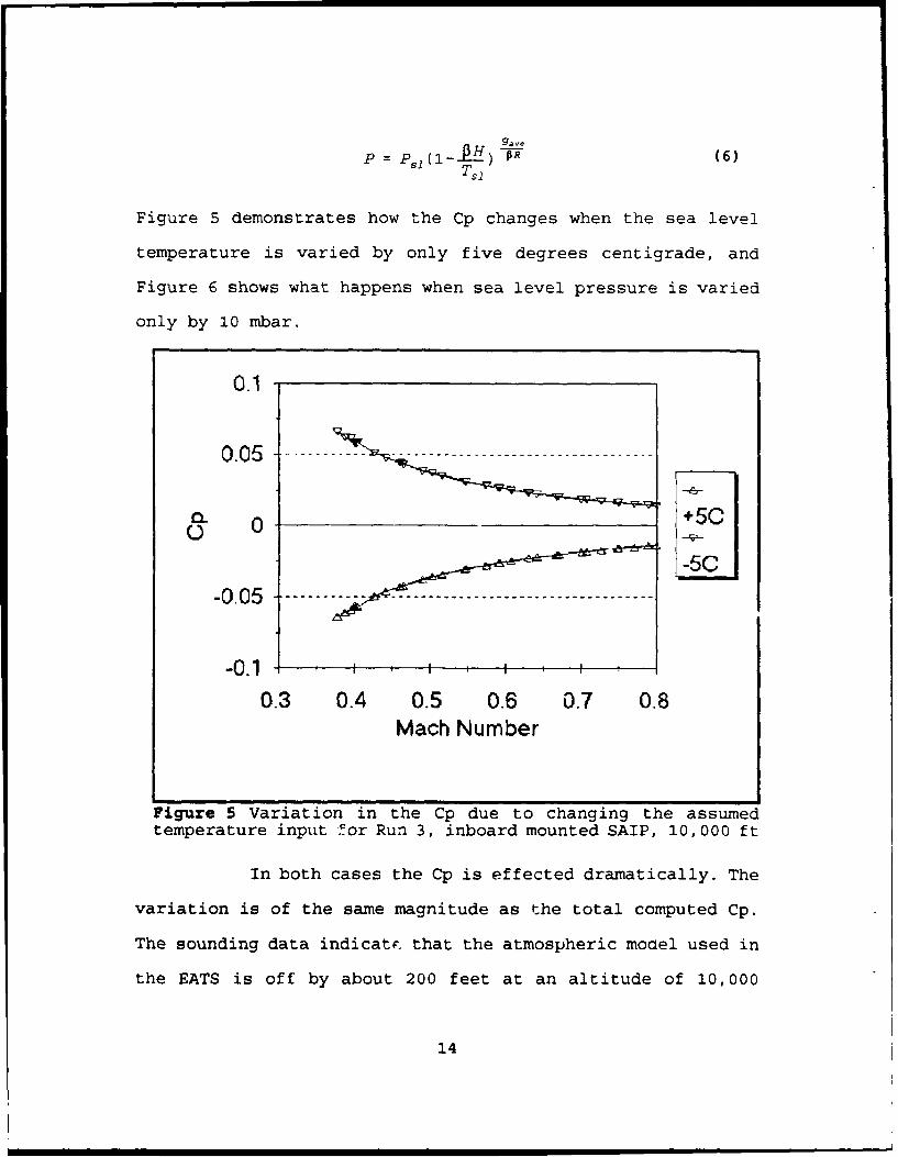
: =ps1(1 - Ti)P (6)
Figure 5 demonstrates how the Cp changes when the sea level
temperature is varied by only five degrees centigrade, and
Figure 6 shows what happens when sea level pressure is varied
only by 10 mbar.
01
0.05 -... ----------------------
0 +5C
-005
-0 .1, , , , , ,
0.3 0.4 0.5 0.6 0.7 0.8Mach Number
Figure 5 Variation in the Cp due to changing the assumedtemperature input for Run 3, inboard mounted SAIP, 10,000 ft
In both cases the Cp is effected dramatically. The
variation is of the same magnitude as the total computed Cp.
The sounding data indicate that the atmospheric moael used in
the EATS is off by about 200 feet at an altitude of 10,000
14

feet depending on the initial conditions were used. The other
400 to 1000 feet of the error along with the variation in the
altitude error is attributed to the aerodynamics.
0.12
0.06 --- ---- -- -- ------ -----
, 0 +10 mbar0O
-10 mbar-0 .0 6 .. .. ---- - --- - --- -- -- -- -- -- -- -
-0.12 I , I
0.3 0.4 0.5 0.6 0.7 0.8Mach Number
Figure 6 Variation in Cp due to changing the assumedpressure input for run 3, inboard mounted SAIP, 10,000 ft
D. AERODYNAMIC CORRECTION
Having defined the limitations and assumptions noted
above, the study proceeds as follows: The static pressures are
computed for the A-6 and the SAIPs, and converted into Cp.
Several methods are used to fit the data in order to define Cp
as a function of Mach rnunber. These include linear,
exponential, logarithmic and power curve fits. The best
15

correction turns out to be the quadratic fit. The SAIP
pressure i' then entered into the altitude equation used by
the A-6 to determine the error due to the aerodynamics alone.
The altitude equation assumes that static pressure is being
read. The static pressure error factor can be rearranged as
follows:
PsAIPP- - (7)~M.-C +1
Using a quadratic estimate for Cp gives:
PSAZPP- = (8)
YM2 (A*M 2 +B*M+C) +1
Where A, B, and C are the coefficients for the quadratic fit
of Cp. The correction then becomes a function of Mach number
only. Although the Cp is actually a function of both Mach
number and angle of attack (AOA), using the Mach number alone
appears to give adequate results.
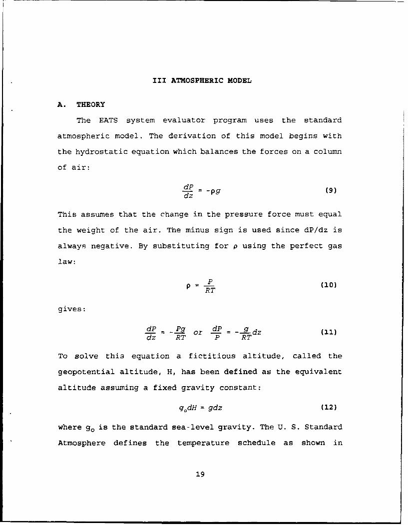
This correction for P. keeps the altitude error below 100
feet. Figure 7 illustrates the improvement in altitude reading
for Run 3. The upper curve shows the error using no correction
for Cp, while the lower curve uses a quadratic correction. The
remainder of the runs are shown in Appendix B. The data for
each SAIP location and altitude were fit to a corresponding
correction curve:
10,000 feet Inboard: 0.6796M2 - 0.9356M + 0.3906
10,000 feet Outboard: 0.1875M2 - 0.2392M + 0.1429
16

4,000 feet Inboard: 0.3393M2 - 0.4251M + 0.1906
4,000 feet Outboard: 0.1239M2 - 0.1077M + 0.0706
1000
8 0 0 -- ------------------ ----------- - ----
Uncorrected
S600
LU 200 --... ........ Cszrreted
0
-2000.35 0.45 0.55 0.65 0.75 0.85
Mach Number
-a-Inboard -e- Outboard
Figure 7 The altitude errors for Run 3 with and without aquadratic approximation for Cp to correct P,, 10,000 feet
The curve for 10,000 feet inboard SAIP location is shown
in Figure 8. The remainder of the curves are plotted in
Appendix B. While these curves produced adequate results for
this study, further flight testing is required to extend the
data base for other aircraft and other altitudes.
17
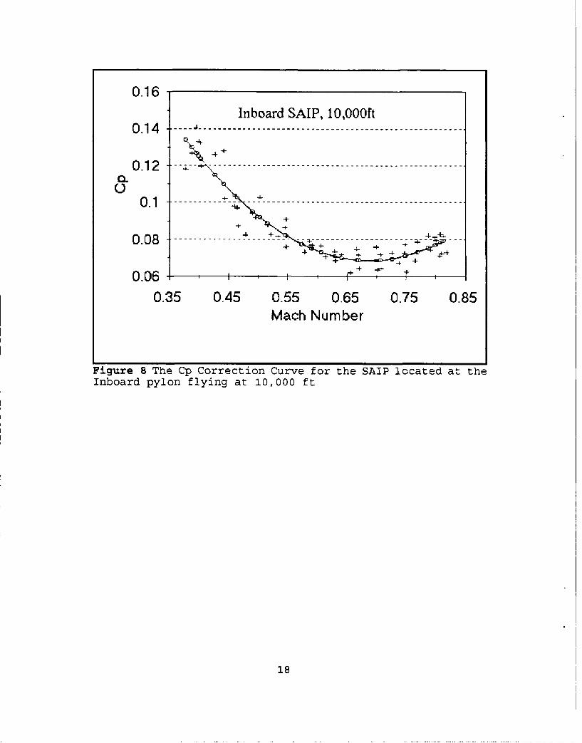
0.16Inboard SAIP, 10,000ft
0.14 --------------------------------------- ----------------
0.12 ---•---------- ...............................................
C-)0 .1 --- - - - - --- - - - - - - - - - - - - - - - - - - - -0 .0 8 --- ------ --------- ----. . . . . . . . . . .. . . . . . . . . .+
+ ++
0.08 ....--- ........... -~---. -
. 4
0.06 + *, I , t0.35 0.45 0.55 0.65 0.75 0.85
Mach Number
Figure 8 The Cp Correction Curve for the SAIP located at theInboard pylon flying at 10,000 ft
18
III ATMOSPHERIC MODEL
A. THEORY
The EATS system evaluator program uses the standard
atmospheric model. The derivation of this model begins with
the hydrostatic equation which balances the forces on a column
of air:
dP _dz Pg
This assumes that the change in the pressure force must equal
the weight of the air. The minus sign is used since dP/dz is
always negative. By substituting for p using the perfect gas
law:
p = P (10)RT
gives:
dP _Pg or dP _ dzdz RT P RT
To solve this equation a fictitious altitude, called the
geopotential altitude, H, has been defined as the equivalent
altitude assuming a fixed gravity constant:
g0dH = gdz (12)
where g. is the standard sea-level gravity. The U. S. Standard
Atmosphere defines the temperature schedule as shown in
19

100- 0< 0 225.66 K
at,04 10-3 XjM109
-165.66 Ka3 -- 4.5 X 10- 3 Kim
447
2I 242.6 8.K
160 20 tepe ., K 280 20
Figure 9 The U. S. Standard Atmosphere Temperature Profile
Figure 9 [Ref. 10]. For this study only the first two regions
will be looked at. The troposphere assumes a constant lapse
rate, fl, of 0.0065 OC/meter up to 11 kilometers (36,000 feet),
and the isothermal region of the stratosphere assumes a
20

constant temperature up to 25 kilometers (82,000 feet).
Therefore the temperature can be expressed as T = To - H.
Substituting this and equation 12 into equation 11 and taking
the integral gives:
P H
P R(TO- (P)
integrating yields:
lnL go-1n( To-1(H)PO in( (14)
solving for P:
9"P =P(l- PTo) ( -• (15)
C TO
or rearranging for altitude:
H= j[1-(-P) 1 (16)0 P0
Above 11 kilometers, in the isothermal region, temperature
is assumed to be a constant Ti., = Tc - 71.50. The altitude is
then computed by:
21

I P + 11,000 (17)go Piso
with Piso being the pressure at the beginning of the
isothermal region.
B. EATS ALTITUDE MODEL
The EATS system evaluator program takes the standard
atmosphere profile developed previously, and enters in the
current pressure and temperature. As described in Chapter II,
these readings come from two sites: San Nicholas Island and
Pt. Mugu. The program then determines which of the two
readings it will use, and converts the values to sea-level
values using the same standard atmosphere profile previously
described. The only difference is that the EATS system uses a
value gave instead of go which is the computed gravity at an
altitude of 22,800 meters (approximately 9.725 for gave
compared to 9.806 for go) [Ref. 8]. While there is no
documentation explaining why this is done, a comparison of the
error experienced by varying the gravity term demonstrated
better accuracy with a smaller value for go. This is shown in
Figure 10 which plots the error versus altitude using three
different values for go. While the error with go equal to
9.725 is still significant, it is typically within the 3%
error specification up through 60,000 feet. Depending on the
severity of the inversion layer, this correction can still
22

fall well outside the specification limit. On days where there
is no significant inversion layer, all three curves remain
within the 3% window.
Altitude Ero' CouWe• Oy 5AIF Altitpae Model1400,POINT "UU
1200. 2152Z 07 S• 1989 9,75
1000
b80O
goo-
400
20
0. ...... _
°0 1 2 3 4 5 6
Alttude X 4
Figure 10 The Effect on Altitude Error of Varying go
C. ALTITUDE ERRORS OF EATS MODEL
The main problem with the standard atmosphere model is
that it does Lot take into account the severe inversion layers
that are prevalent at Pt Mugu. Although only minor altitude
errors occurred (1000 feet at an altitude of 45,000 feet) on
days showing a standard temperature profile , virtually every
sounding examined was non-standard. Without examining the
23

profile, there is no way of knowing how severe the errors will
be. Most days there was an inversion layer profile. The
temperature decreases steadily until an altitude of about
1,000 feet. The temperature suddenly jumps 100 C and then
decreases steadily until it hits the isothermal region. Also
it is not uncommon for the isothermal region to start at
50,000 feet, which is considerable higher than the standard
36,000 feet. Another profile started with a positive lapse
rate for the first few thousand feet, and then the temperature
decreased steadily giving only three regions. Figures 11 and
12 show some typical temperature profiles with the
corresponding errors in altitude predictions. The model
typically predicts well until an inversion layer is
encountered, then the altitude error jumps to 800-1,400 feet
at an altitude of 30,000 feet. Above 60,000 feet, the altitude
error can exceed 3,000 feet.
D. METHODOLOGY TO CORRECT EATS MODEL
Several methods were attempted to bring the atmospheric
model within specifications. All the methods bring the
estimate closer than the current model, but all required
operator intervention.
This investigation built on the work of Mr. Anthony A.
Terrameo, Jr. of NAWCWPNS, Pt. Mugu [Refs. 11 and 12]. The
atmospheric model proposed by Mr. Terrameo in these reports
corrects the errors due to the inversion layer, and provides
24

Temperature Profile3020 SAN NICOLAS IS
10 2030Z 05 SEP 1989
0-• -10
-20
-30I--
-40-
-50
-60
-70801 2 3 4 5 b
Altitude X1 04
1200 .......... . .NIIN OLAS IS.... . .. . .
2030Zi 05 SEP 1g•9 , .
1 0 0 0 ..... ....... ... ........ . ... ... .... ..... .... . . . .
00 . ............ .......... .. .... .......... .... ....b Currernt' Model
L..
600. . .
2R 0 0 -.. ........ . .. .• . .. .. .. o r e t e .. . . . ... . . ... .... ...... .. .. .... . .. . . . .. . ..f, a t a p e r t s'
20 ........... ...Corrected for actual iopse rdtes
0 1 2 3 4 5
Altitude xl 04
Figure 11 Typical Temperature Profile for the Pt. Mugu AreaCompared to Standard Temperature Profile Along WiLh theAltitude Errors Caused by the Inversion Layer and the ErrorsWith a Corrected Model
25

Temperature Profile20 '
10 SAN NICOLAS IS
1340Z 19SEP 19890
-10
-20-
-30
~-40-
-50-
-60 - \ .- -
-70-70 1 2 3 5 6
Altitude X1 04
moo SAN N COLAS IS .. .......-.
................... ...........
13'40Z :19 SEP 1989 ,B O O -.................... ... ...... ...... .... .. ......... . . .. . .. -- -" . . ., ' ' . . . . . ... .. .
! /
S/~600
/ Current Model
400 - 7 -
.•~ ~~~ .... .......... ... .../." "" ° .... . . i - • ... . ..~~ ~~............. .. .... . .. .. . . . . . ... . . . .
2 0 .. . . .....
0 1 Crrted..for .. C.tual. Ipse rates..... ..... ... ... .-. ....
-200 1* -.- - - -. - - .
0 1 2 3 4 5 6
Attitude xi 10
Figure 12 A Temperature Profile with only a Mild InversionLayer and the Altitude Errors it Causes.
26

an accurate profile for altitude. The benefit of the methods
presented here is reduced computation time at the expense of
increased operator involvement.
The foundation for all the methods developed here is to
divide the atmosphere into a four section model and compute
actual lapse rates for temperature based on the sounding data
provided by the Geophysics Department at NAWCWPNS, Pt. Mugu.
The first region extends from the earth's surface to the
bottom of the inversion layer. The second region covers the
inversion layer. The third region stretches from the top of
the inversion layer to the isothermal region. The final region
covers the isothermal layer. Sounding data must be examined to
define these regions. The temperature and pressure at each
transition point is recorded, and the lapse rate is determined
by linear regression for each section.
The first model uses the measured temperature and pressure
and the computed lapse rates as follows: The regions are
defined by the pressure, and an altitude is computed for each
transition point. To determine which region the aircraft is
in, and which equation to use, the pressure read from the SAIP
is compared to the pressure read at each transition point.
Each equation uses the temperature and pressure measured at
the beginning of the region, and the lapse rate for the
region. The altitude computed by the equation is added to the
altitude computed for the bottom of the region to determine
the total altitude. The third program in Appendix A
27

demonstrates how this was accomplished using MATLAB. This
worked very well for most days to bring the error down from
over 1,400 teet to under 250 feet at an altitude of 30,000
feet. The method does require the sounding data to be manually
examined to pick out the layer. When a program was written to
do this automatically, several temperature profiles would fool
the program into making the wrong breaks. A more sophisticated
program could possibly work more effectively, but manual
intervention will still likely be required.
The locations chosen for the transition points has a large
effects on the errors in the model. Depending on where the
layer was placed, the error would vary from under 100 feet up
to 600 feet. This can be seen by comparing the correction
shown in Figure 13 to the correction in Figure 12. The only
difference between the two figures is the definition of the
temperature regions. For Figure 12, the breaks are at: 15,000,
23,000 and 50,000 feet. Figure 13 used altitude breaks of:
5,000, 5500, and 50,000 feet. The second and third programs in
Appendix A plot the temperature profile so the altitude breaks
for each section can be entered. An iteration process is used
to achieve an optimum profile. This method did not work
particularly well with profiles with only three distinct
sections, but it could easily be rewritten to accommodate
this. The lower graphs in Figures 11 and 12 demonstrate this
correction method.
28

1000 '- ... ".- ..... "
134Z 19 SEP 19Pi9800 . ...... . ,
600 ........... L .......... . Current Mode
400 -X
-2 0 0 1 . ....... ...... ........ ...' -"r . ......... .... - .. C 'r e t M d•......... ...... . .. ... . . .......
- 41 0 0 l- .... ....... . .. , . .. . . . . ... . ...... ....... ......... . .. . ... ... . .. .. . ..
-a 0 0 .............. .... ............. ...... ... .... .... .... ... ... ...... . .....
0 1 2 3 4 5 6
Altitude x1O4
Figure 13 The altitude error for a corrected atmosphericmodel using the wrong transition points.
One profile caused significant problems. It consisted of
a large jump in temperature at the surface, and then proceeded
with a standard inversion layer profile. It was assumed that
the first datum point in the sounding was bad. The method
worked fine after the surface temperature reading was altered
to fit a four -ection profile.
The next method is identical to the above, except that
both pressure and altitude are used to define each section.
Instead of using a computed altitude added to each section,
the actaal altitude for that region, as recorded from the
sounding data is used. This has the advantage of bringing the
error to zero at the beginning of each section. Unfortunately,
29

this profile has considerable discontinuities, which cause the
altitude to jump as the aircraft passes through each
transition layer.
A third method computes the gravity constant for the
average altitude in each region. This gravity term is used in
each equation, and true altitude is produced rather than
geopotential altitude. This method worked well, but did not
produce any better accuracy than the first method. The
advantage is in computational time. The gravity term is
computed once, while in the other methods geopotential
altitude must be converted into true altitude for each
reading. Figure 14 shows the result of this method which
reduced the error from 1,100 feet to under 150 feet.
30

200: SAN NICOLAS IS
174,5Z 19 SEP 1989
150 " 3
D Altitude Error using model corrected forvanrble raovity and octudO lops* rctes.
0 2 34 5
Attitude ,104
Figure 14 The Altitude Error Using True Lapse Rates and anAverage go for each region.
31

IV. CONCLUSIONS AND RECOMMENDATIONS
A. CONCLUSIONS
This study evaluated the possibility of correcting the
altitude determination error of the SAIP by using Cp to
correct the aerodynamic errors and using a modified
atmospheric model to correct for the effects of the inversion
layers experienced at Pt. Mugu. It was demonstrated that this
combination is a viable solution to the SAIP's altitude
problems.
Assuming that Cp is a function of Mach number alone gives
errors under 100 ft for all velocities from Mach 0.4 to Mach
0.8. Changing the atmospheric model for the conditions at Pt.
Mugu by incorporating the sounding data from the Geophysics
Department at NAWCWPNS, Pt. Mugu will allow the EATS system
evaluator program to determine the actual altitude to within
200 ft up through an altitude of 60,000 ft. The Geophysics
Department has indicated that the soundings can be scheduled
for any event, and data can be reduced and sent to the EATS
center within two hours of the data being taken. Both
corrections are simple to add to the current program, and
effectively correct the altitude problems with a minimum of
expense, since no hardware modifications are required. More
flight test data must be reduced for the Cp correction curves,
32

but the method is straightforward. Although the Cp was
computed as a function of mach number and altitude, the data
also displayed a definite dependence on either AOA or vertical
velocity. Either could be added into the equation for a better
fit.
B. RECOMMENDATIONS
The atmospheric model should be modified promptly to more
accurately predict altitude. The correction to the software is
relatively simple, and there would be no increase in the real
time computing. A program must be written to view the
temperature profile received from the Geophysics Department,
and to plot the altitude error so the best profile can be
entered. Rather than using several models and selecting the
best model for the day, one model that can accommodate several
regions using the actual lapse rates would be adequate, and
much easier to fit to any temperature profile.
The aerodynamic correction will not be as straightforward.
Implementing the correction once it is determined is easy;
determining the correction is not. Any flight measurement
could be used which has raw pressure, Mach number, altitude,
and vertical velocity or AOA available. The data must be
analyzed to determine Cp as a function of mach number, and
altitude. Vertical velocity or AOA could be added depending on
which is more readily available to develop a better correction
33

curve. If no data exists with these parameters, then future
flight tests must be set up to extract this information.
The SAIP could still be a viable altitude determining
resource if these corrections are implemented. Although the
geopositional satellite system (GPS) is to be implemented in
the future, the SAIP is likely to be in use for the next
several years.
34

APPENDIX A: MATLAB PROGRAMS
A. PROGRAM TO SHOW EFFECT OF VARYING gave"
This program varies the gravity term used in the EATS
equation to show the effect of using the gave value for 22,800
meters. All of the equations here are in a single line in the
actual program, but have been split into two lines here when
necessary.
% This program takes an input file of the sounding data, and% plots it using three values for gave-
A=size(HTP); % HTP is the sounding dataH=[] ; % (Height, Temperature,HG= []; % Pressure)M2F=3.28083989501; % Conversion for meters to feetRad=6348407*M2F; % Earths radius as supplied byRadl=6348407*M2F*9.80665/9.795707; % Geophysics Dept.Gave=9.806; G='9.806';Tu=HTP(i,2)+273.15 - 0.0065*(11000-HTP(1,1)/M2F);Pu=HTP(I,3)*(I- ((.0065*(II000-HTP(I,I)/M2F))/
(HTP(I,2)+273.15)))A(Gave/1.86576);
for I=1:A(l),if HTP(I,3)>Pu,
H(I,I)=((HTP(I,2)+273.15)/.0019812)* (i-(HTP(I,3)/HTP(1,3)) . (1.86576/Gave))+HTP(1,1);
else,H(I,I)=-(M2F*287.04*Tu/Gave)*(log(HTP(I,3)/Pu)) +
11000*M2F;end;
end;HG=Rad*H./(Radl-H);ERROR=HTP (:, 1) -HG;
plot(HTP(:,1),HTP(:,2))title('Temperature Profile')xlabel ('Altitude')
ylabel ('Temperature C')gtext ('')
35

plot (HTPC: ,l) ,ERROR)xlabel ('Altitude')ylabel('Altitude Error ft')title('Altitude Error caused by SAIP Altitude Model')gtext (NAME)gtext (DATE)gtext (G)
Gave=9 .75;G=' 9.75';Pu=HTP (1,3) * (1-((.0065* (11000-HTP (1,1) /M2F)) /
(HTP (1, 2) +273.15) ) )A(Gave/i. 86576);
for I=l:A(l),if HTP (1,3) >Pu,
HTP (1, 3) ).A(1. 86576/Gave) )+HTP (1, 1)else,
H(I,l)=-(M2F*287.O4*Tu/Gave)*(log(HTP(I,3)/Pu)) +1l000*M2F;
end;end;
HG=Rad*H. /(Radl-H4);ERROR=HTP (: ,l) -HG;hold;plot (HTP(: ,l) ERROR)gtext (G)
Gave=9.725;G='9.725';
(HTP (1,2) +273 .15) ))A (Gave/i. 86576);
for I=l:A(1),if HTP(I,3)>Pu,
HTP (1, 3) ).A(1. 86576/Gave) )+HTP (1,1);else,H(I,1)=-(M2F*287.04*Tu/Gave)*(log(HTP(I,3)/Pu)) +
11000*M2F;end;
end;HG=Rad*H. /(Radl-H);ERROR=HTP C: ,1)-HG;plot (HTP (: ,1),ERROR)gtext (G)
plot (HTP(: ,l),HTP (:,1) * *3, '.
mneta graphi
hold;
36

B. PROGRAM TO PLOT ALTITUDE ERROR USING A VARIABLE gave
This program computes an average gave for each section of
the atmosphere and uses that to calculate actual altitude,
instead of using a single gave and then converting the
geopotential altitude into actual altitude. The input file of
the sounding data is analyzed to break up the atmosphere into
four sections, and the gravity for the average altitude for
each section is computed. Due to the great variance that can
be seen in temperature profiles, the data has to be examined
manually.
M2F=3.28083989A=size(HTP);TO=HTP(I,2)+273.15;PO=HTP(I,3);H0=HTP(1,1);R=287.04;GSL=9.7957;H=[];P3=0;RAD=20820807;axis((0,5000,0,30]);temp % temp is a program to plot theaxis; % temperature profile, so the altitudetemp % breaks can be determined.HT=input('enter the altitude bieaks: ');
TEST=l; % The breaks are determined, andfor I=1:A(1), % constants initialized
if TEST==1,if HTP(I,1)>HT(1) & HTP(I,2)<HTP(I+l,2),
T1=HTP(I,2)+273.15;P1=HTP(I,3);HI=HTP(I,I);B=polyfit(HTP(l:I,l),HTP(1:I,2),l);BO=-B(l);TEST=2;B=I;
37

G1=GSL* (RADJA2/ (RAD+H1/2) A2);end
elseif TEST==2,if HTP(I,1)>HT(2) & HTP(I,2)>HTP(.I-1,.2),
T2=HTP(I,2) +273.15;P2=HTP (I, 3);H2=HTP (I, 1);B=polyfit(HTP(B:I,1) ,HTP(B:I,2) ,1)B1= -B (1)TEST=3;B=I;G2=GSL* (RADAA2/ (R.AD+ (H1+H2) /2) A2);
endelseif TEST==3,
if HTP (1,1) >HT(3) ,B=polyfit(HTP(B:I,1),HTP(B:I,2),1);B2=-B (1)TEST=4;P3=HTP (I, 3);H3=HTP (I, 1);B=I-1;G3=GSL* (P.AA2/ (RAD+ (H2+H3)/2 )A 2);
endelseend
endT3=ave(HTP(B:A(I),2)) + 273.15;G4=GSL*(R.ADA*2/(RAD+(H3+HTP(A(1) ,1))/2 )A2);
for I=1:A(1),if HTP(I,3) >= P1,H(I)=(TO/BO)*(1-(HTP(I,3) /pO)A (R*M2F*BO/G1))+HO;
elseif HTP(I,3) >= P2,H1 (TO/Ba)* (1- (P1/PO) A (R*M2F*BO/G1) )+HO;
elseif HTP(I,3)>= P3,H2= (Ti/Bi) * (1-(P2/Pi )A (R*M2F*B1/G2) )+H1;H(I)=(T2/B2)*(1-(HTP(I,3)/P2 )A (R*M2F*B2/G3))+H2;
elseH3=(T2/B2)*(1l (P3/P2 )A (R*M2F*B2/G3))+H2;H(I)= -((T3*R*M2F/G4)*log(HTP(I,3)/P3)) + H3;
endendERROR=HTP(:,1) -H';
axis( [O,HTP(A(l) ,1),min(ERROR) -5O,max(ERROR)+50]);plot (HTP (:,1) , RROR,HTF (:,1),0. u3*HTP (: , 1) , '
xlabel ('Altitude')ylabel('Altitude Error ft')atext('Altitude Error using model corrected for,)
38

gtext('variable gravity and actual lapse rates.')gtext (NAME)gtext (DATE)gtext('3%'')
meta graphl
C. PROGRAM TO PLOT ALTITUDE ERROR USING ACTUAL LAPSE RATES.
This program computes plots the temperature profile so the
transition points can be extracted. The program determines the
actual transitions above the first two points chosen, and then
uses the third point as the actual break for the isothermal
region. The temperature and pressure are read off for the
start of each region, and a lapse rate is computed for the
first three regions. The actual lapse rates are used to
compute altitude, along with the temperature and pressure
measured at each transition point. The altitude is computed
for each transition point and added to the computed altitude
for each section to determine total altitude.
% This takes an input file of the sounding data, and plots it.
M2F=3f.28083989501;Rad=6348407*M2F;Radl=6348407*M2F*9.80665/9.795707;A=size (HTP);H=[];R=287.04;Gave=9.7257954;
Tu=HTP(1,2)+273.15 - 0.0065*(II000-HTP(1,1)/M2F);iPu-HTP([i, 3) *(I- ((. 0065* (II000-HTP(I, I)/M2,) )/ (HTP (I,2) +273.15)))Gave/1.86576);
39

for I=l:A~l),if HTP (1,3) >Pu,
(1.865-/6/Gave) )+HTP(l,l);else,
H(I,l)~=-(M2F*287.04*Tu/Gave)*(log(HTP(I,3)/Pu)) +
ll000*M2F;end;
end;HG=Rad*H./(Radl-H);ERROR1=HTP (: ,l) -HG;
axis( [0,5000,0,30]);plot(HTP(:,l) ,HTP(:,2))gtext( Uaxis;plot(HTP(:,l),HTP(:,2))title('Temperature Profile')xlabel ('Altitude')ylabel ('Temperature C')gtext (NAME)gtext (DATE)meta graphlHT=input('enter the altitude breaks:')%plot(IHTP(:,I),ERROR)%xlabel ('Altitude')%ylabel('Altitude Error ft')t title('Altitude Error caused by SAIP Altitude Model')It gtext (NAME)%gtext (DATE)%meta graphl
TQ=HTP (1,2) +273 .15;PO=HTP(1,3);P=l;for I=1:A(l),
if P==i,if HTP(I,1)>HT(l) & HTP(I,2)<HTP(I+l,2),
Tl=HTP(I,2) +273 .15;P1=HTP (I, 3);B=polyfit(HTP(l:I,1) ,HTP(1:I,2) ,1)BO=-B(l);P=2;B=I;
endelseif P==2,
if HTP(I,l)>HT(2) & HTP(I,2)>HTP(I+1,2),T2=HTP(I,2) +273.15;P2 =HTP (1,3);B=polyfit(HTP(B:I,1),HTP(B:I,2),1);
40

B1= -B (1)P=3 ; B=I;
endelseif P==3,
if HTP(I,1)>=HT(3),T3=ave(HTP(I:A(1),2)) + 273.15;P3=HTP (I, 3);B=polyfit(HTP(B:I,1),HTP(B:I,2),l);B2= -B (1)P=4;
endelseend
end
for I=1:A(1),if HTP(I,3) >= P1,
H(I)=(TO/BO)*(l-(HTP(I,3)/PO)A(R*3.28O84*BO/Gave))+HTP(l,l);elseif HTP(I,3) >= P2,
H1= (TO/BO) *(1- (P1/Pa) A(R*3 .28084*BO/Gave) )+HTP (1,1);H(I)=(Tl/B1)*(l-(HTP(I,3)/P1)A"(R*3.28O84*Bl/Gave))+H1;
elseif HTP(I,3) >= P3,H2=(IT/Bl)*(l-(P2/Pl)A(R*3.28O84*Bl/Gave))+Hl;H(I)=(T2/B2)*(1-(HTP(I,3)/P2)A(R*3.28O84*B2/Gave))+H2;
H3=(T2/B2)*(1-(P3/P2)A'(R*3.28O84*B2/Gave))+H2;H(I)=-M2F*R*T3/Gave*log(HTP(I,3)/P3) + H3;
endend
HG=Rad*H./(Rad1-H);ERROR=~HTP (: ,1)-HG;
axis( [O,HTP(A(1) ,l) ,min(min(ERROR),rnin(ERROR1))-50,max(max(ERROR), max(ERROR1))+503);
plot(IiTP(:,l),ERROR,HTP(:,l),O.03*HTP(:,l), .,
xlabel ('Altitude')ylabel('Altitude Error ft')gtext ('Current Model')gtext('Corrected for actual lapse rates')gtext (NAME)gtext (DATE)gtext ('3%')gtext('3%'l)gridmeta graphiaxis;
41

APPENDIX B. GRAPHS OF AERODYNAMIC DATA
300-
0
-1 00 , , , ICorrected
0.35 0.45 0.55 0.65 0.75 0.85
Mach Number
-- Inboard -e- Outboard
Figure 15 Corrected and Uncorrected Altitude Errors for theSAIP for Run 2, 4,000 ft
42
1000
600400 -..-----------------
W J 2 0 0 --- ------------ . C -Q r c• € t e d -----------------------L. 0
-2000.35 0.45 0.55 0.65 0.75 0.85
Mach Number
-8-Inboard -e- Outboard
Figure 16 Corrected and Uncorrected Altitude Errors for theSAIP for Run 3, 10,000 ft
43

850
6 5 0 ------- ---
~ 450 - Uncorrected0
L . 2 5 0 . . ..- --- -----
Corrected5 0 . •- _---- - - - - --.• _ _----------------
-150
0.35 0.45 0.55 0.65 0.75 0.85Mach Number
-- Ibar-3 OutboardI
Figure 17 Corrected and Uncorrected Altitude Errors For theSA:P for Run 4, 4,000 ft
44

900
700 -----------------------------
g 50---Uncorrected
u 300 -- _---0
Corrected100 ---------------------------------------------------
-100
0.4 0.5 0.6 0.7 0.8Mach Number
-a-Inboard -e- Outboardi
Figure 18 Corrected and Uncorrected Altitude Errors for theSAIP for Run 5, 10,000 ft
45

0.1Inboard SAIP, 4,000 ft
0~
4--
++
4--
+++ .4- +
• -4-
0.04 , I i I
0.35 0.45 0.55 0.65 0.75 0.85Mach Number
Figure 19 Quadratic Curve Fit to the Data for Cp for theInboard Station at 4,000 ft
46
0.08
Outboard SAIP, 4,000
4-,t
0 .0 4 - - -. . . . . . . . . . . . . .. . . . . . . . . . .44-
-4--4.-
0.020.35 0.45 0.55 0.65 0.75 0.85
Mach Number
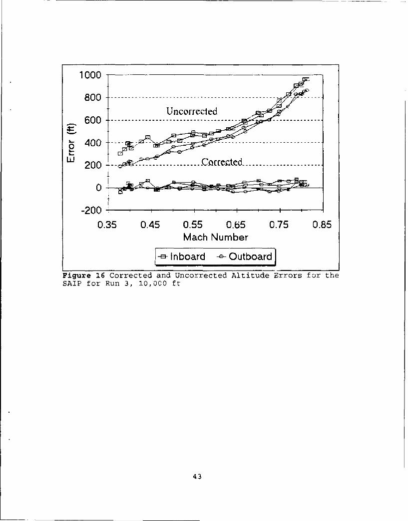
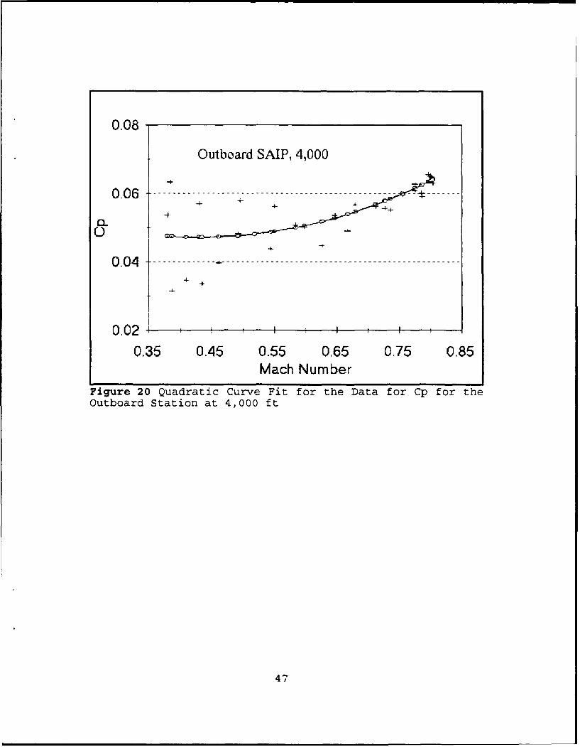
Figure 20 Quadratic Curve Fit for the Data for Cp for theOutboard Station at 4,000 ft
47

0.16Inboard SAIP, 1O,00ft
0.14 4 . .--- --------------------------------------------------------
0 .1 2 - . -.-.-.---------- --------- --------- --------- --------t'-4
0~0 .1 . . . . . . . . -+ - - ------- ------------------------------------
++0 .0 8 - . . . . . . .----- _--- ---- -- - ---- -- --- ;-- •-- _---.----
-+ 4-
0.06 I ,+ +
0.35 0.45 0.55 0.65 0.75 0.85Mach Number
Figure 21 Quadratic Curve Fit for the Data for Cp for theInboard Station at 10,000 ft
48

0.085Outboard SAIP, 10,000 It
0 .0 8 . . . ..- - . . . . . . . . . . ..-- ,- . . . . . . . . . . ..-- - - - - - - - - - - - - - - - - - - - - - - - - - - - -
- 4.0 .0 7 5 --- -------- .-- -----" --------- ----- --------------------" --- -4 -C -+.44--.-
0 .0 7 _- --- -- -- ---------------------------------...... ......--_
0+ 064 -+-
++
-I-I
-4-4
0.075 - ------------------------------
+ 4.
.4-
0.06 - i , , , ,
0.35 0.45 0.55 0.65 0.75 0.85Mach Number
Figure 22 Quadratic Curve Fit for the Data for Cp for theOutboard Station at 10,000 ft
49
LIST OF REFERENCES
1. Eastburg, S. R., An Engineering Study of AltitudeDetermination Deficiencies of the Service AircraftInstrumentation Package (SAIP), Aeronautical Engineer'sThesis, Naval Postgraduate School, Monterey, California,December 1991.
2. Russell, R. J., A Continuing Study of AltitudeDetermination Deficiencies of the Service AircraftInstrumentation Package (SAIP), Master's Thesis, NavalPostgraduate School, Monterey, California, September 1991.
3. Rixey, J. W., A Multi-faceted Engineering Study ofAerodynamic Errors of the Service Aircraft InstrumentationPackage (SAIP), Aeronautical Engineer's Thesis, NavalPostgraduate School, Monterey, California, September 1992.
4. Function Specification for the Service InstrumentationPackage (SAIP), Pacific Missile Test Center SpecificationPMTC-CD-EL-697-76A, 31 March 1989.
5. McCue, J. J., Pitot-static Systems, Classroom Notes, U. S.Naval Test Pilot School, Patuxent River, Maryland, March 1990.
6. Huston, W. B., Accuracy of Airspeed Measurements and FlightCalibration Procedures, NACA Report No. 919, Langley Field,Va, May 16,1946.
7. A-6E Block 1A E250.00 Annotated Math Flows, A-6E Branch,Code 3192, Naval Weapons Center, China Lake, Ca, 21 February1992
8. Terrameo, A. A., Jr., Hydrostatic Altitude Model, TechnicalNote No. 3450-23-87, Pacific Missile Test Center, Point Mugu,California, May 1987.
9. Air Data Computer (ADC) Output Correction to A-6E PI El1OProgram For Both Old (T32) and New Box (T58), NATC, PatuxentRiver, Maryland, 23 March 1978.
10. Wallace, J. M., Hobbs, P. V., Atmospheric Science, AnIntroductory Survey, Academic Press, New York, New York, 1977.
11. Terrameo, A. A., Jr., EATS Altitude Errors Caused ByTemperature Inversion Layers, Technical Note No. 3452-10-91,Pacific Missile Test Center, Point Mugu, California, February1991.
50
12. Terrameo, A. A., Jr., Altitude Errors Caused ByTemperature Inversion Layer Modeling Errors in the EATSHydrostatic Model, Technical Note No. 3452-11-91, PacificMissile Test Center, Point Mugu, California, May 1991.
51
INITIAL DISTRIBUTION LIST
No. Copies1. Defense Technical Information Center 2
Cameron StationAlexandria VA 22304-6145
2. Library, Code 052 2Naval Postgraduate SchoolMonterey CA 93943-5002
3. Chairman 1Department of Aeronautics, Code AANaval Postgraduate SchoolMonterey, CA 93943-5000
4. Mr. Brian Frankhauser 1Naval Air Warfare Center, Weapons DivisionCode P3611Point Mugu, CA 93042-5001
5. Mr. Guy Cooper 1Naval Air Warfare Center, Weapons DivisionCode 9054Point Mugu, CA 93042-5001
6. Mr. William Harrington 1Naval Air Warfare Center, Weapons DivisionCode 3421.4Point Mugu, CA 93042-5001
7. Mr. Rick Navarro 1Naval Air Warfare Center, Weapons DivisionCode P3611Point Mugu, CA 93042-5001
8. Mr. Antony Terrameo, Jr. 1Naval Air Warfare Center, Weapons DivisionCode P3615Point Mugu, CA 93042-5001
9. Mr. Ron Ornay 1Naval Air Warfare Center, Weapons DivisionCode P36111Point Mugu, CA 93042-5001
52

10. Mr. John LoosNaval Air Warfare Center, Weapons DivisionCode P3611Point Mugu, CA 93042-5001
11. Prof. Oscar BiblarzDepartment of Aeronautics, Code AA/BiNaval Postgraduate SchoolMonterey, CA 93943-5000
12. LCDR Joseph SweeneyDepartment of Aeronautics, Code AA/SwNaval Postgraduate SchoolMonterey, CA 93943-5000
13. LT Daniel SergentOPS/OC Div.USS Nimitz (CVN-68)FPO AP 96697-2820
53