A Computational Study of the Soot Formation in Methane-Air … · A Computational Study of the Soot Formation in Methane-Air Diffusion Flame During Early Transience Following Ignition

Abstrdevelopand nummethanethe flamtill the symmetcentral (non-prsimulatidistribudestructoxidatioimportawith theheights respecticoncentof surfathan thignitionenrichedimportaparticlefractionpatternsduring t

Indexoxidatio

ManusBijan K

Bengal EIndia (phoyahoo.co.

AmitavUniversityamdatta@

AmitavJadavpur stutul@re

Soot combusmortalit

Engineering Letters, 16:3, EL_16_3_04______________________________________________________________________________________

A Computational Study of the Soot Formation in Methane-Air Diffusion Flame During Early

Transience Following Ignition

Bijan Kumar Mandal, Amitava Datta, and Amitava Sarkar

act— A CFD-based numerical model has been ed for the determination of the volume concentration

ber density of soot in a laminar diffusion flame of in air, under transient condition following ignition of e. The transience is studied from the point of ignition final steady state is reached. The burner is an axi-ric co-flowing one with the fuel issuing through a port and air through an annular port. Both normal air eheated) and preheated air have been used for this on to capture the effect of preheating on soot tion. Attention is focused on various soot forming and ion processes, like nucleation, surface growth and n, during the transient phase to evaluate their relative nce. The transient soot distribution has been studied help of radial distributions of soot at six different axial of 2 cm, 4 cm, 6 cm, 8 cm, 10 cm and 12 cm

vely above the burner tip. Beyond 12 cm height, the ration becomes very less in all cases. The contribution ce growth towards soot formation is more significant at of nucleation during the early periods following . Once the high temperature reaches the oxygen- zone beyond the flame, the soot oxidation becomes

nt. Coagulation, on the other hand, limits the soot number. Preheating of air increases the soot volume in the flame significantly. But, the soot distribution remain almost similar to that with non-preheated air he flame transient period and also in the steady state.

Terms—air preheating, laminar diffusion flame, n, soot, Transient modeling

cript received October 31, 2007. umar Mandal is with the Mechanical Engineering Department,

ngineering and Science University, Shibpur, Howrah 711 103,ne: 91 033 26887619; fax: 91 033 26684561; e-mail: bkm375@

in). a Datta is with the Department of Power Engineering, Jadavpur, Salt Lake Campus, Kolkata 700098, India (e-mail:hotmail.com). a Sarkar is with the Mechanical Engineering Department,

University, Kolkata 700 032, India (e-mail:diffmail.com).

I. INTRODUCTION is an atmospheric pollutant formed in hydrocarbon tion, which causes respiratory illness and increases y. Soot in flame results from incomplete combustion

of hydrocarbons in the reducing atmosphere, where enough oxygen is not available to yield a complete conversion of fuel to carbon di-oxide and water vapour. According to to Haynes and Wagner [1], pyrolysis of hydrocarbon fuel molecules break them up into smaller hydrocarbons and finally to acetylene. The initial step of the formation of soot is the production of aromatic species from the aliphatic hydrocarbons, e.g. acetylene. The aromatic species grow by combining with other aromatic and alkyl species to form large polyaromatic hydrocarbons (PAH), which itself is carcinogenic. Continued growth of PAH molecules eventually lead to the smallest identifiable soot particles. Soot particles in flame also play a major role in heat transfer from the flame. Therefore, better understanding and control of soot forming processes in hydrocarbon combustion are required.

Non-premixed or diffusion flames are sooty in nature. Practical diffusion flames are mostly turbulent, however, the study of laminar diffusion flames still finds importance because of their fundamental nature and due to the fact that the turbulent diffusion flames can be taken as an aggregate of laminar flamelets. Wey et al. [2], Santoro et al. [3], Smooke et al. [4], Lee et al. [5] and Xu et al. [6] performed experiments in laminar diffusion flames using various hydrocarbon fuels for the determination of soot. Wey et al. [2] found that the soot volume fraction and aggregate diameters increased with the height above the burner, while the opposite was the case with number densities. Santoro et al. [3] experimented with various fuels, viz. ethane, ethene and propane at different fuel and air flow rates. It was observed that the increase in soot formation is primarily due to an increase in the residence time in the annular region of the diffusion flame. Smooke et al. [4] measured the soot volume fraction as well as the concentrations of fuel (methane), acetylene and benzene within the flame zone of a co-flowing laminar jet diffusion flame. Lee et al. [5] observed that the rate of soot inception became stronger with the oxygen enriched oxidizer stream. However, the soot yield in the flame zone was lower with higher oxygen in the oxidizer.

Semi-empirical models, based on simple description of soot chemistry, have shown much promise in the prediction

(Advance online publication: 20 August 2008)

of soot in diffusion flames. Smith [7] proposed a model that assumed particle inception entirely due to physical nucleation. Gore and Faeth [8] calculated soot volume fraction in turbulent diffusion flame based on mixture fraction. Kennedy et al. [9] used a one-equation model for the conservation of soot volume fraction to describe the soot formation and oxidation in an ethylene-air laminar diffusion flame. Leung et al. [10] used a simple kinetic model to predict soot volume fraction in co-flow and counter-flow laminar diffusion flames. It was assumed in their model that acetylene is primarily responsible for the nucleation and growth of soot particles. Rate of nucleation was assumed to be first order in C2H2 concentration, while the rate of surface growth was assumed first order in C2H2 and also dependent on the aerosol surface area. Said et al. [11] postulated a hypothetical intermediate species between the fuel and soot and used two rate equations for the formation and oxidation of the intermediate species and soot respectively. Syed et al. [12] considered surface growth to be a function of the aerosol surface area, while Moss et al. [13] took it to be dependent on number density. Nucleation, coagulation and oxidation were taken care of using suitable model parameters in both the models and model constants were calibrated for different fuels. Smooke et al. [4] considered the soot formation rate to be a function of acetylene, benzene, phenyl and molecular hydrogen concentrations. Surface growth rate was calculated based on acetylene concentration.

Oxidation of soot is another important issue, which controls its emission level. Lee et al. [14] measured the oxygen and temperature dependence of oxidation of soot in a laminar diffusion flame. Another widely used model of soot oxidation was due to Nagle and Strickland-Constable [15]. However, their measurement did not directly correspond to flame situation. Najjar and Goodger [16] modified the rate constants of Nagle and Strickland-Constable to improve the prediction capability of the rate equation in flames.

Almost all the works on soot production in laminar diffusion flames have been done on steady diffusion flames under different operating conditions and fuels. In turbulent diffusion flames local extinction and re-ignition of flame is observed, on which not much work has yet been done. Recently, Mitarai et al. [17] developed a lagrangian flamelet model for the description of this phenomenon. Sripakagorn et al. [18] studied the effect of Reynolds number on the local extinction and re-ignition of the diffusion flame. The soot formation behaviour in the flame front can be entirely different during flame development in a mixture following ignition compared to that in a steady flame. No work has yet been done on this aspect and therefore, the topic needs attention. Other transient flame applications, e.g. during lighting up of a burner flame and flame development in a diesel engine, are available where the flame is not steady and the behaviour can only be explained by doing a transient modeling of the flame development and pollutant formation. Therefore, it would be very interesting to investigate the

development of soot volume fraction in a transient and moving flame following the ignition process.

With this motivation, soot formation during the transient development phase of a confined, co-flowing, laminar jet diffusion flame following ignition has been studied numerically in the present work. A CFD based numerical code has been developed for the purpose, which solves the transient governing equations based on an explicit finite difference technique. Methane is considered to be the fuel and the choice is made because it constitutes more than 90% of natural gas. The combustion of fuel is simulated by a two-step equation for simplification. The soot models of Syed et al. [12] and Moss et al. [13] are employed with the necessary adjustments for the sake of compatibility with the present combustion model. Governing equations for soot volume fraction and number density are solved along with the equations of mass, momentum, energy and gas phase species concentrations. The radiative energy transport in the flame is neglected. It is reported by Mohammed et al. [19] and Zhu and Gore [20] that the maximum temperature changes by about 50-75 K when the gas phase radiation is not considered in a steady, laminar, co-flowing methane/air diffusion flame model. Sivathanu and Gore [21] reported that in methane/air diffusion flame the soot radiation is weaker than the gas phase radiation. Zhu and Gore [20] have also made a comprehensive analysis to study the influence of radiation on temperature and soot formation in a methane/air diffusion flame at different pressure. It is reported that in an atmospheric pressure flame, the effect of radiation on temperature is small (within 50 K) and on the peak soot volume fraction is negligible. Supply of preheated air in the combustor is used in many applications as a means of heat recovery [22]. As a result, the temperature and oxidizer concentration change, which affect the flame structure (flow characteristics, temperature and species concentration fields) and emission of pollutants like soot, CO and NO. Literature lacks studies of soot formation with preheated air. Hence the effect of air preheating on soot formation has also been studied under transient condition.

II. MODEL FORMULATION

A. Reacting Flow Model An axi-symmetric laminar diffusion flame in a confined

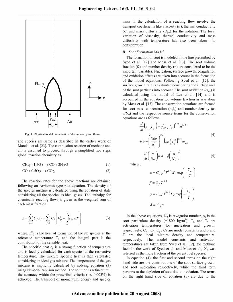
physical environment is considered with fuel (methane) admitted as a central jet and air as a co-flowing annular jet. The schematic diagram of the physical model of the diffusion flame above the burner tip has been shown in Fig.1. The inner fuel tube diameter is 12.7 mm and the outer tube diameter is 50.4 mm. The combustion process is simulated with a detailed numerical model, which is developed for solving the transient governing equations for a laminar, reacting flow with appropriate boundary conditions along with the formation of soot. The flow is vertical through the reaction space and the gravity effect is included in the momentum equation.

The conservation equations for mass, momentum, energy



and species are same as described in the earlier work of Mandal et al. [23]. The combustion reaction of methane and air is assumed to proceed through a simplified two steps global reaction chemistry as

O22HCO21.5O4CH +→+ (1)

2CO20.5OCO →+ (2) The reaction rates for the above reactions are obtained

following an Arrhenius type rate equation. The density of the species mixture is calculated using the equation of state considering all the species as ideal gases. The enthalpy for chemically reacting flows is given as the weighted sum of each mass fraction

⎟⎟⎟

⎠

⎞

⎜⎜⎜

⎝

⎛+== ∫∑∑

==

T

T

pjfj

n

jjj

n

jj

o

dTchChCh 0

11

(3)

where, h0

fj is the heat of formation of the jth species at the reference temperature T0 and the integral part is the contribution of the sensible heat.

The specific heat cp is a strong function of temperature and is locally calculated for each species at the respective temperature. The mixture specific heat is then calculated considering an ideal gas mixture. The temperature of the gas mixture is implicitly calculated by solving equation (3) using Newton-Raphson method. The solution is refined until the accuracy within the prescribed criteria (i.e. 0.003%) is achieved. The transport of momentum, energy and species

mass in the calculation of a reacting flow involve the transport coefficients like viscosity (µ), thermal conductivity (λ) and mass diffusivity (Djm) for the solution. The local variation of viscosity, thermal conductivity and mass diffusivity with temperature has also been taken into consideration.

df Air Fuel Air

z

r

Flame

B. Soot Formation Model The formation of soot is modeled in the line prescribed by

Syed et al. [12] and Moss et al. [13]. The soot volume fraction (fv) and number density (n) are considered to be the important variables. Nucleation, surface growth, coagulation and oxidation effects are taken into account in the formation of the model equations. Following Syed et al. [12], the surface growth rate is evaluated considering the surface area of the soot particles into account. The soot oxidation (ωox) is calculated using the model of Lee et al. [14] and is accounted in the equation for volume fraction as was done by Moss et al. [13]. The conservation equations are formed for soot mass concentration (ρsfv) and number density (as n/N0) and the respective source terms for the conservation equations are as follows:

( ) ( )

( ) ox/

vs

/

s

//vsvs

ωfnρρπ

δ

nfργfρdt

d

3122

31

2

3132

36⎟⎟⎠

⎞⎜⎜⎝

⎛−+

=

(4)

2

00⎟⎠⎞

⎜⎝⎛−=⎟

⎠⎞

⎜⎝⎛

Nnβα

Nn

dtd (5)

where,

⎟⎟⎠

⎞⎜⎜⎝

⎛−=

TT

XTρCα αc

.α exp502

50.βTCβ =

⎟⎟⎠

⎞⎜⎜⎝

⎛−=

T

TXρTCγ γ

c.

γ exp50

αCδ δ=

In the above equations, N0 is Avogadro number, ρs is the

soot particulate density (=1800 kg/m3), Tα and Tγ are activation temperatures for nucleation and growth, respectively, Cα , Cβ, Cγ , Cδ are model constants and ρ and T are the local mixture density and temperature, respectively. The model constants and activation temperatures are taken from Syed et al. [12], for methane fuel. In the work of Syed et al. and Moss et al., Xc was referred as the mole fraction of the parent fuel species.

In equation (4), the first and second terms on the right hand side are the contributions of the soot surface growth and soot nucleation respectively, while the third term pertains to the depletion of soot due to oxidation. The terms on the right hand side of equation (5) are due to the

Fig. 1. Physical model: Schematic of the geometry and flame.



contribution of nucleation and coagulation, respectively. The nucleation and surface growth terms account for the chemical phenomena through Arrhenius type rate equation. The coagulation term is derived from the Smolushowski equation for coagulation of liquid colloids [24].

Conservation equations for the soot mass concentration and number density are solved in the present model along with the gaseous species in the solution domain. As soot particles do not follow the molecular diffusion theory, the diffusion velocities in the soot conservation equations are replaced by the corresponding thermophoretic soot particle velocities. Therefore, the conservation equations, in general, can be expressed

( ) ( )

( ) ( ) φztrt

zr

SφVz

φrVrr

φρvz

φrvrrt

φ

&+∂∂

+∂∂

=

∂∂

+∂∂

+∂∂

1

1

(6)

The above equation is applicable both for the soot mass concentration (ρsfv) and number density (n/N0) and accordingly ϕ will assume the respective variable value.

The thermophoretic velocity vector ( ) has been calculated following Santoro et al. [3] as

tV

( ) TT

υ

πξ/Vt ∇

+=

814

3 (7)

where, the accommodation factor (ξ) has been taken as unity. Equations (4) and (5) form the source terms ( ) of the conservation equations of the soot mass concentration and number density, respectively. The soot volume fraction is obtained from the mass concentration solution.

φS&

III. SOLUTION METHODOLOGY

A. Numerical Scheme The gas phase conservation equations of mass,

momentum, energy and species concentrations along with the conservation equations of soot mass concentration and number density are solved simultaneously, with their appropriate boundary conditions, by an explicit finite difference computing technique taking into account the transient terms in the equations. The algorithm is based on the SOLA scheme proposed by Hirt and Cook [25] and modified in certain aspects as described in Datta [26] and Mandal et al. [23]. The variables are defined following a staggered grid arrangement. The advection terms are discretised following a hybrid differencing scheme, based on cell Peclet number, while the diffusion terms are discretised by the central differencing scheme. The solution is explicitly advanced in time satisfying the stability criteria that the grid Fourier number stays within limit (< 0.5). In every time step, first the axial and radial momentum equations are solved. Pressure corrections and the associated corrections of velocities to satisfy the conservation of mass

are then done by an iterative scheme. The enthalpy transport and the species transport equations, including those of soot variables, are subsequently solved within the same time step. The temperature is decoded from the enthalpy and species concentration values by Newton-Raphson method. Transient results at desired intermediate time are achieved in the process of time advancement. The process continues till a steady state convergence is reached and the final solution simulates a steady flame.

B. Boundary Conditions Boundary conditions at the inlet are given separately for

the fuel stream at the central jet and the air stream at the annular co-flow. The streams are considered to enter the computational domain as plug flow, with velocities calculated from their respective flow rates. The temperatures of fuel and air are specified. In conformation with the conditions used by Mitchell et al. [27], the fuel flow rate is taken as 3.71 × 10-6 kg/s and the air flow rate is taken as 2.214 × 10-4 kg/s. The temperatures for both the streams are 300 K in case of non-preheated air. The temperature for preheated air is taken to be 400 K. The inlet velocities are calculated from the respective mass flow rates and densities of air and methane fuel. No soot is considered to enter with the flow through the inlet plane. Considering the length of the computational domain to be 0.3 m, the fully developed boundary conditions for the variables are considered at the outlet. In case of reverse flow at the outlet plane, which occurs in the case of buoyant flame, the stream coming in from the outside is considered to be atmospheric air. Axi-symmetric condition is considered at the central axis, while at the wall a no-slip, adiabatic and impermeable boundary condition is adopted.

C. Grid Size A variable size adaptive grid system is considered with

higher concentration of nodes near the axis, where larger variations of the variables are expected. However, the variations in the size of the grids are ensured to be gradual. Grid testing is done by several variations of the number of grids in either direction. It is observed that the increase in the numbers of grids in the z×r directions from 85×41 to 121×61 almost doubles the computation time, but the maximum change in results is within 2%, which is checked for the maximum velocity, temperature and peak soot volume fraction. Hence a numerical mesh with 85×41grid nodes is finally adopted.

D. Stability Criteria The choice of the incremental time-step has to be done

very carefully as it is directly related to the stability of the explicit scheme. The restrictions suggested by Hirt et al. [28] are used here. The first criteria demands that pure advection should not convey a fluid element past a cell in one time increment as the difference equations consider fluxes only between adjacent cells. Hence the time increment should satisfy the following inequality.



v

δz,

v

δrδt

zr ⎭⎬⎫

⎩⎨⎧

< min1 (8)

The second constrain puts a restriction on the grid Fourier

number, such that the fluxes should not diffuse more than one cell length in one time increment. This restriction on the incremental time is imposed through the following condition.

{ } ( ) δzδr

δzδrDα,ν,max

0.5δt 22

22

2+

×< (9)

Incremental time-step using both the criteria is calculated

for all the cells in the entire domain. Finally, the incremental time-step is chosen considering both the criteria together and it is given by

{ } δt,δtminδt 21= (10)

However, during the computation, the actual values of δt

are suitably scaled down in order to ensure the convergence of the problem.

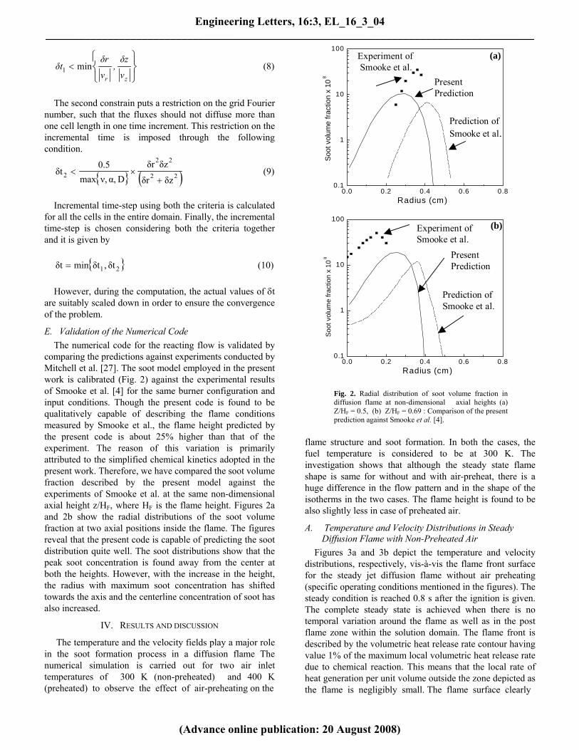
E. Validation of the Numerical Code The numerical code for the reacting flow is validated by

comparing the predictions against experiments conducted by Mitchell et al. [27]. The soot model employed in the present work is calibrated (Fig. 2) against the experimental results of Smooke et al. [4] for the same burner configuration and input conditions. Though the present code is found to be qualitatively capable of describing the flame conditions measured by Smooke et al., the flame height predicted by the present code is about 25% higher than that of the experiment. The reason of this variation is primarily attributed to the simplified chemical kinetics adopted in the present work. Therefore, we have compared the soot volume fraction described by the present model against the experiments of Smooke et al. at the same non-dimensional axial height z/HF, where HF is the flame height. Figures 2a and 2b show the radial distributions of the soot volume fraction at two axial positions inside the flame. The figures reveal that the present code is capable of predicting the soot distribution quite well. The soot distributions show that the peak soot concentration is found away from the center at both the heights. However, with the increase in the height, the radius with maximum soot concentration has shifted towards the axis and the centerline concentration of soot has also increased.

IV. RESULTS AND DISCUSSION

The temperature and the velocity fields play a major role in the soot formation process in a diffusion flame The numerical simulation is carried out for two air inlet temperatures of 300 K (non-preheated) and 400 K (preheated) to observe the effect of air-preheating on the

flame structure and soot formation. In both the cases, the fuel temperature is considered to be at 300 K. The investigation shows that although the steady state flame shape is same for without and with air-preheat, there is a huge difference in the flow pattern and in the shape of the isotherms in the two cases. The flame height is found to be also slightly less in case of preheated air.

A. Temperature and Velocity Distributions in Steady Diffusion Flame with Non-Preheated Air

Figures 3a and 3b depict the temperature and velocity distributions, respectively, vis-à-vis the flame front surface for the steady jet diffusion flame without air preheating (specific operating conditions mentioned in the figures). The steady condition is reached 0.8 s after the ignition is given. The complete steady state is achieved when there is no temporal variation around the flame as well as in the post flame zone within the solution domain. The flame front is described by the volumetric heat release rate contour having value 1% of the maximum local volumetric heat release rate due to chemical reaction. This means that the local rate of heat generation per unit volume outside the zone depicted as the flame is negligibly small. The flame surface clearly

0.0 0.2 0.4 0.6 0.80.1

1

10

100

Soot

vol

ume

fract

ion

x 10

8

Experiment of Smooke et al.

Present Prediction

Prediction of Smooke et al.

(a)

Radius (cm)

0.0 0.2 0.4 0.6 0.80.1

1

10

100

Soo

t vol

ume

fract

ion

x 10

8

Radius (cm)

Experiment of Smooke et al.

Present Prediction

Prediction of Smooke et al.

(b)

Fig. 2. Radial distribution of soot volume fraction indiffusion flame at non-dimensional axial heights (a)Z/HF = 0.5, (b) Z/HF = 0.69 : Comparison of the presentprediction against Smooke et al. [4].



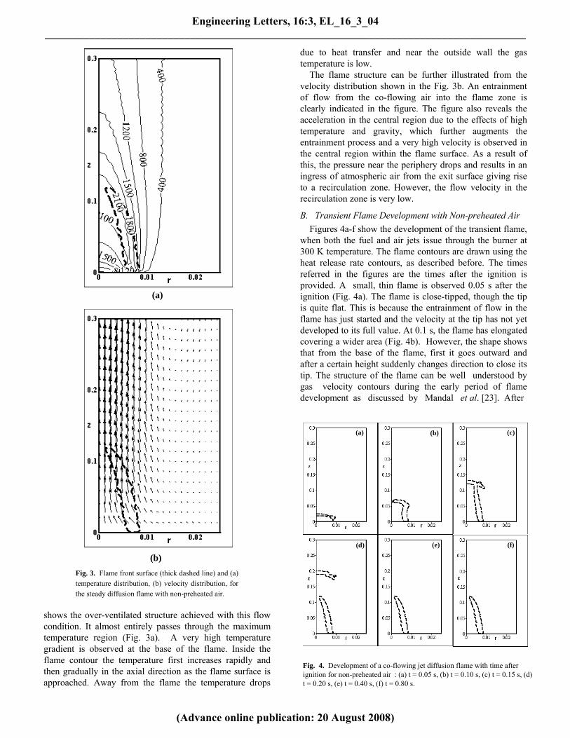
shows the over-ventilated structure achieved with this flow condition. It almost entirely passes through the maximum temperature region (Fig. 3a). A very high temperature gradient is observed at the base of the flame. Inside the flame contour the temperature first increases rapidly and then gradually in the axial direction as the flame surface is approached. Away from the flame the temperature drops

due to heat transfer and near the outside wall the gas temperature is low.

The flame structure can be further illustrated from the velocity distribution shown in the Fig. 3b. An entrainment of flow from the co-flowing air into the flame zone is clearly indicated in the figure. The figure also reveals the acceleration in the central region due to the effects of high temperature and gravity, which further augments the entrainment process and a very high velocity is observed in the central region within the flame surface. As a result of this, the pressure near the periphery drops and results in an ingress of atmospheric air from the exit surface giving rise to a recirculation zone. However, the flow velocity in the recirculation zone is very low.

B. Transient Flame Development with Non-preheated Air Figures 4a-f show the development of the transient flame,

when both the fuel and air jets issue through the burner at 300 K temperature. The flame contours are drawn using the heat release rate contours, as described before. The times referred in the figures are the times after the ignition is provided. A small, thin flame is observed 0.05 s after the ignition (Fig. 4a). The flame is close-tipped, though the tip is quite flat. This is because the entrainment of flow in the flame has just started and the velocity at the tip has not yet developed to its full value. At 0.1 s, the flame has elongated covering a wider area (Fig. 4b). However, the shape shows that from the base of the flame, first it goes outward and after a certain height suddenly changes direction to close its tip. The structure of the flame can be well understood by gas velocity contours during the early period of flame development as discussed by Mandal et al. [23]. After

(a)

(a) (b) (c)

(d) (e) (f)

d)

(b) Fig. 3. Flame front surface (thick dashed line) and (a)temperature distribution, (b) velocity distribution, forthe steady diffusion flame with non-preheated air.

Fig. 4. Development of a co-flowing jet diffusion flame with time after ignition for non-preheated air : (a) t = 0.05 s, (b) t = 0.10 s, (c) t = 0.15 s, (t = 0.20 s, (e) t = 0.40 s, (f) t = 0.80 s.



0.15s, the flame shape almost takes the conventional over-ventilated structure, but a small wing is also observed (Fig. 4c). The wing in the flame is to consume any fuel, which earlier escaped out with the flow. At 0.2 s, the main flame, established above the burner rim (Fig. 4d), takes the shape of the steady flame. However, at this time a second flame is also observed much above the main flame. This is due to burning of the escaped fuel through the central region before the flame is established. The fuel, which has left the central zone when the flame was not established, moves downstream with relatively slower velocity and mixes with oxygen to form a combustible mixture. The establishment of the main flame accelerates the high temperature product gases. It subsequently catches the cool flammable gas mixture, ignites it and causes the second flame to set in. However, the second flame is only temporary and extinguishes as all the escaped fuel burn or move out of the domain. Therefore, at 0.4 s only the main flame is seen (Fig. 4e) without any additional secondary flame. The results of 0.4 s and 0.8 s (Fig. 4f) do not show any difference in the flame structure. This shows that the flame reaches its stable position even before 0.4 s. However, developments and adjustments in the post flame zone continue with the mixing and transport of gases beyond the flame and the fully steady condition in the entire solution domain is only observed after 0.8 s.

C. Soot Distribution in Transient Flame with Non-Preheated Air

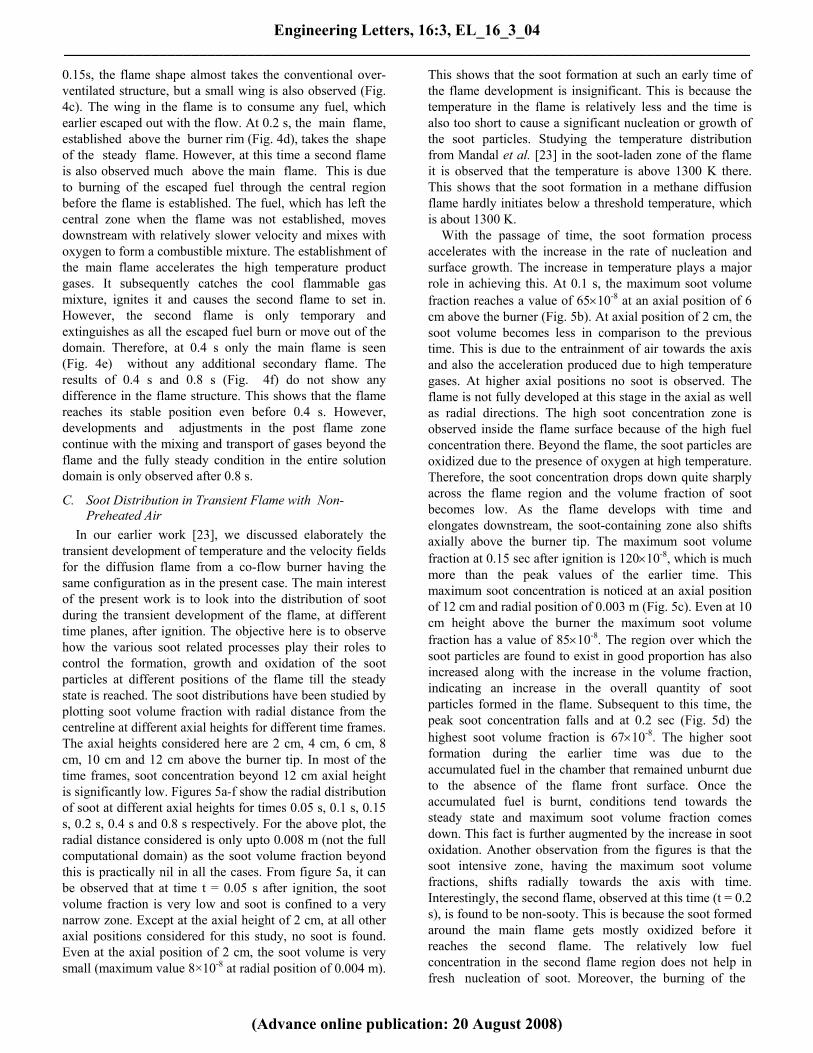
In our earlier work [23], we discussed elaborately the transient development of temperature and the velocity fields for the diffusion flame from a co-flow burner having the same configuration as in the present case. The main interest of the present work is to look into the distribution of soot during the transient development of the flame, at different time planes, after ignition. The objective here is to observe how the various soot related processes play their roles to control the formation, growth and oxidation of the soot particles at different positions of the flame till the steady state is reached. The soot distributions have been studied by plotting soot volume fraction with radial distance from the centreline at different axial heights for different time frames. The axial heights considered here are 2 cm, 4 cm, 6 cm, 8 cm, 10 cm and 12 cm above the burner tip. In most of the time frames, soot concentration beyond 12 cm axial height is significantly low. Figures 5a-f show the radial distribution of soot at different axial heights for times 0.05 s, 0.1 s, 0.15 s, 0.2 s, 0.4 s and 0.8 s respectively. For the above plot, the radial distance considered is only upto 0.008 m (not the full computational domain) as the soot volume fraction beyond this is practically nil in all the cases. From figure 5a, it can be observed that at time t = 0.05 s after ignition, the soot volume fraction is very low and soot is confined to a very narrow zone. Except at the axial height of 2 cm, at all other axial positions considered for this study, no soot is found. Even at the axial position of 2 cm, the soot volume is very small (maximum value 8×10-8 at radial position of 0.004 m).

This shows that the soot formation at such an early time of the flame development is insignificant. This is because the temperature in the flame is relatively less and the time is also too short to cause a significant nucleation or growth of the soot particles. Studying the temperature distribution from Mandal et al. [23] in the soot-laden zone of the flame it is observed that the temperature is above 1300 K there. This shows that the soot formation in a methane diffusion flame hardly initiates below a threshold temperature, which is about 1300 K.

With the passage of time, the soot formation process accelerates with the increase in the rate of nucleation and surface growth. The increase in temperature plays a major role in achieving this. At 0.1 s, the maximum soot volume fraction reaches a value of 65×10-8 at an axial position of 6 cm above the burner (Fig. 5b). At axial position of 2 cm, the soot volume becomes less in comparison to the previous time. This is due to the entrainment of air towards the axis and also the acceleration produced due to high temperature gases. At higher axial positions no soot is observed. The flame is not fully developed at this stage in the axial as well as radial directions. The high soot concentration zone is observed inside the flame surface because of the high fuel concentration there. Beyond the flame, the soot particles are oxidized due to the presence of oxygen at high temperature. Therefore, the soot concentration drops down quite sharply across the flame region and the volume fraction of soot becomes low. As the flame develops with time and elongates downstream, the soot-containing zone also shifts axially above the burner tip. The maximum soot volume fraction at 0.15 sec after ignition is 120×10-8, which is much more than the peak values of the earlier time. This maximum soot concentration is noticed at an axial position of 12 cm and radial position of 0.003 m (Fig. 5c). Even at 10 cm height above the burner the maximum soot volume fraction has a value of 85×10-8. The region over which the soot particles are found to exist in good proportion has also increased along with the increase in the volume fraction, indicating an increase in the overall quantity of soot particles formed in the flame. Subsequent to this time, the peak soot concentration falls and at 0.2 sec (Fig. 5d) the highest soot volume fraction is 67×10-8. The higher soot formation during the earlier time was due to the accumulated fuel in the chamber that remained unburnt due to the absence of the flame front surface. Once the accumulated fuel is burnt, conditions tend towards the steady state and maximum soot volume fraction comes down. This fact is further augmented by the increase in soot oxidation. Another observation from the figures is that the soot intensive zone, having the maximum soot volume fractions, shifts radially towards the axis with time. Interestingly, the second flame, observed at this time (t = 0.2 s), is found to be non-sooty. This is because the soot formed around the main flame gets mostly oxidized before it reaches the second flame. The relatively low fuel concentration in the second flame region does not help in fresh nucleation of soot. Moreover, the burning of the



0.000 0.002 0.004 0.006 0.0080

10

20

30

40

50

60

70(a)

z = 2 cm

f V x 1

08

Radial distance (m)

0.000 0.002 0.004 0.006 0.0080

10

20

30

40

50

60

70(b)

z = 2 cm

z = 4 cm

z = 6 cm

f v x 1

08

Radial distance (m)

0.000 0.002 0.004 0.006 0.0080

20

40

60

80

100

120 (c)

z = 2 cmz = 4 cm

z = 6 cm

z = 8 cm

z = 10 cm

z = 12 cm

f V x1

08

Radial distance (m)

0.000 0.002 0.004 0.006 0.0080

10

20

30

40

50

60

70(d)

z = 12 cm

z = 10 cm

z = 8 cm

z = 6 cm

z = 4 cm

z = 2 cm

f V x 1

08

Radial distance (m)

0.000 0.002 0.004 0.006 0.0080

10

20

30

40

50

60

70(e)

z = 12 cm

z = 10 cm

z = 8 cm

z = 6 cm

z = 4 cm

z = 2 cm

f V x 1

08

Radial distance (m)

0.000 0.002 0.004 0.006 0.0080

10

20

30

40

50

60

70(f)

z = 12 cm

z = 10 cm

z = 8 cm

z = 6 cm

z = 4 cmz = 2 cm

f V x 1

08

Radial distance (m)

Fig. 5. Radial soot distributions at different axial heights with non- preheated air under transient conditions at (a) t =0.05 s, (b) t = 0.10 s, (c) t = 0.15 s, (d) t = 0.20 s, (e) t = 0.40 s, (f) t = 0.80 s.



escaped fuel takes place in the premixed mode producing no soot as it gets time to mix with the entrained oxygen. The above discussion highlights the importance of residence time in the formation of soot in flames. The kinetics of soot formation is slower than that of chemical reaction. Therefore, the soot takes more time to form. Until, such time has elapsed, the concentration of soot remains rather low in spite of the development of the flame. However, the accumulation of fuel in the reacting zone will tend to increase the soot concentration, thereby increasing the maximum soot volume fraction. Once sufficient time is given, the location of the soot-laden zone will change according to the change in the flame shape and structure, but the peak concentration hardly changes any more (after 0.2 s in the present case). The soot distributions at different axial positions at 0.4 and 0.8 s after ignition are similar (figures 5e and 5f). The flame reaches its steady state before 0.4 s, and the transience in the domain continues till 0.8 s only because of adjustments above the flame region. The soot formation primarily occurs inside the flame region. Therefore, the soot distribution does not change much once the flame becomes stable. The illustrations in the last three figures show that soot volume fractions fall sharply beyond 10 cm height. The soot volume fraction values are quite low at 12 cm height compared to that at 10 cm height, the maximum value being 22×10-8. Beyond this outside the flame (flame height being around 11 cm) the particles get oxidized subsequently, because of the high temperature and oxygen in the core. But in cases where such favourable conditions are not available, significant release of soot from the flame will result.

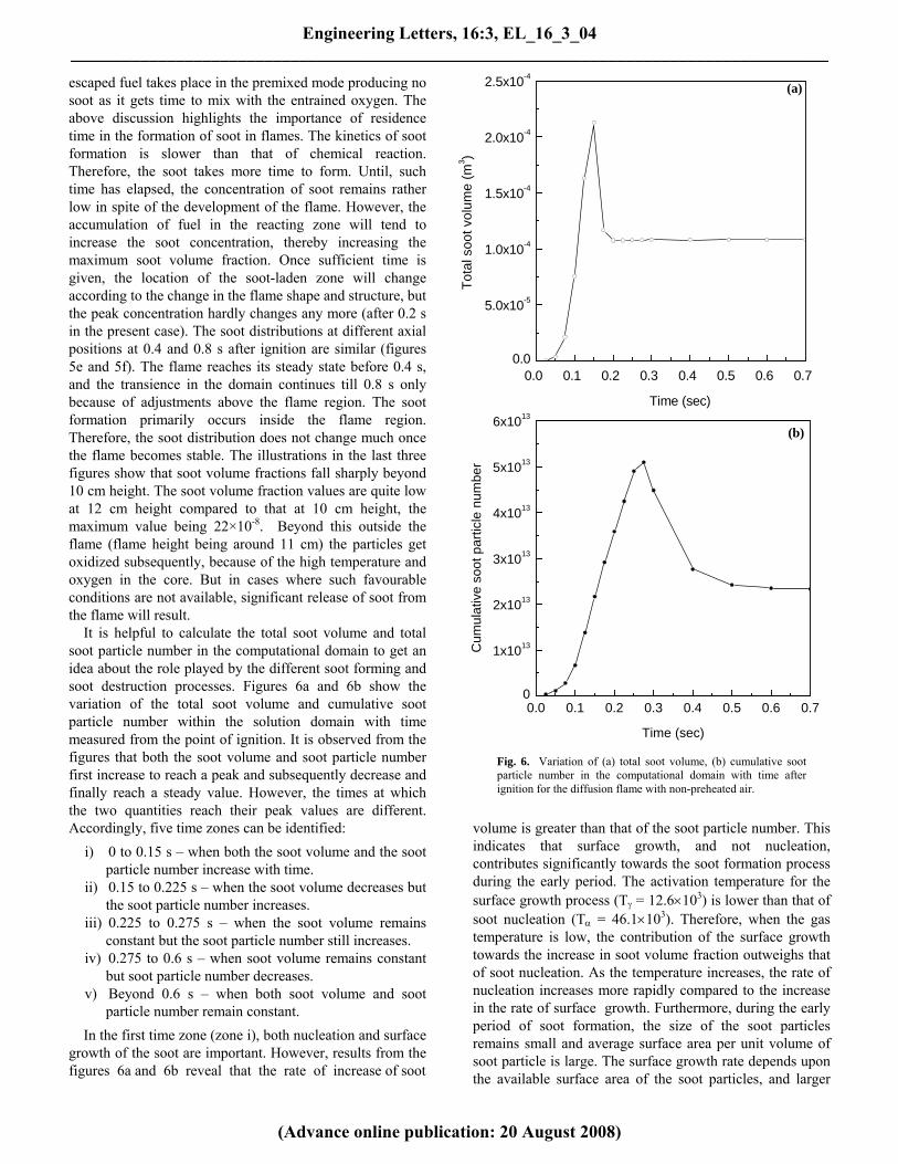
It is helpful to calculate the total soot volume and total soot particle number in the computational domain to get an idea about the role played by the different soot forming and soot destruction processes. Figures 6a and 6b show the variation of the total soot volume and cumulative soot particle number within the solution domain with time measured from the point of ignition. It is observed from the figures that both the soot volume and soot particle number first increase to reach a peak and subsequently decrease and finally reach a steady value. However, the times at which the two quantities reach their peak values are different. Accordingly, five time zones can be identified:

i) 0 to 0.15 s – when both the soot volume and the soot particle number increase with time.

ii) 0.15 to 0.225 s – when the soot volume decreases but the soot particle number increases.

iii) 0.225 to 0.275 s – when the soot volume remains constant but the soot particle number still increases.

iv) 0.275 to 0.6 s – when soot volume remains constant but soot particle number decreases.

v) Beyond 0.6 s – when both soot volume and soot particle number remain constant.

In the first time zone (zone i), both nucleation and surface growth of the soot are important. However, results from the figures 6a and 6b reveal that the rate of increase of soot

0.0

5.0x10-5

1.0x10-4

1.5x10-4

2.0x10-4

2.5x10-4

volume is greater than that of the soot particle number. This indicates that surface growth, and not nucleation, contributes significantly towards the soot formation process during the early period. The activation temperature for the surface growth process (Tγ = 12.6×103) is lower than that of soot nucleation (Tα = 46.1×103). Therefore, when the gas temperature is low, the contribution of the surface growth towards the increase in soot volume fraction outweighs that of soot nucleation. As the temperature increases, the rate of nucleation increases more rapidly compared to the increase in the rate of surface growth. Furthermore, during the early period of soot formation, the size of the soot particles remains small and average surface area per unit volume of soot particle is large. The surface growth rate depends upon the available surface area of the soot particles, and larger

0.0 0.1 0.2 0.3 0.4 0.5 0.6 0.7

Tot

al s

oot v

olum

e (m

3 )

0.0 0.1 0.2 0.3 0.4 0.5 0.6 0.70

13

13

13

13

13

13

(a)

Time (sec)

1x10

2x10

3x10

4x10

5x10

6x10

Cum

ulat

ive

soot

par

ticle

num

ber

Time (sec)

(b)

Fig. 6. Variation of (a) total soot volume, (b) cumulative sootparticle number in the computational domain with time afterignition for the diffusion flame with non-preheated air.



surface area results in faster surface growth during the initial period. After 0.15 s, a high temperature is found and soot oxidation takes a very important role. Though the number of soot particles increases due to further nucleation, but oxidation overcomes the surface growth to cause a decrease in the total soot volume (zone ii). The soot surface growth is a function of the aerosol area and with the formation of more soot particles surface growth rate increases. It finally equals the soot oxidation rate and soot volume reaches a steady value (zone iii). When many soot particles are formed in the domain, coagulation plays a major part. This is because coagulation is directly proportional to the square of the soot number density. Coagulation does not change the soot volume in the domain but reduces the number of particles within it (zone iv). Finally, all the processes attain a state such that both the total soot volume and aggregate soot particle number reach their steady values.

D. Effect of Air Preheat on Soot formation The effect of air preheating on soot formation has been

studied by increasing the temperature of co-flowing air from 300 K to 400 K. In this case, the complete steady state in the whole domain is attained 3.2 s after the ignition is given. The changes in the flame and flow characteristics play a major role on the soot formation process due to air preheating. A detailed discussion on the change in the flow pattern and temperature distribution with preheated air for the present flame condition was presented in Mandal et al. [23]. However the steady state temperature velocity and distributions have been described below.

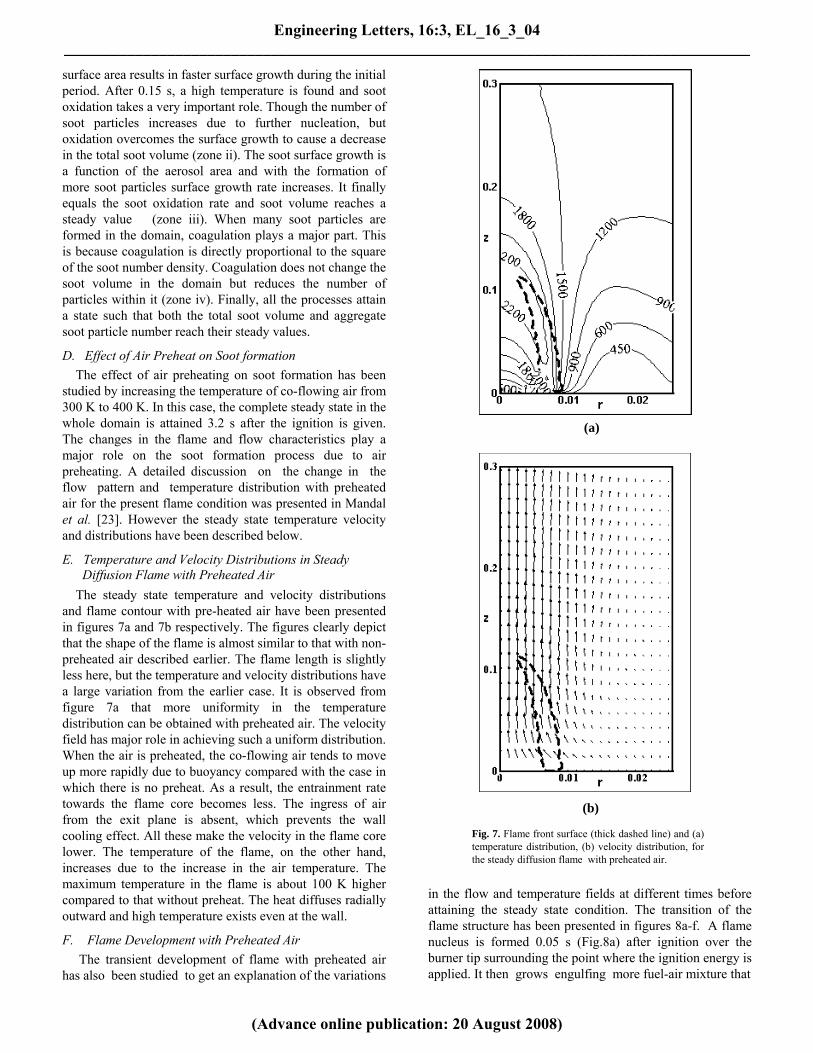
E. Temperature and Velocity Distributions in Steady Diffusion Flame with Preheated Air The steady state temperature and velocity distributions

and flame contour with pre-heated air have been presented in figures 7a and 7b respectively. The figures clearly depict that the shape of the flame is almost similar to that with non-preheated air described earlier. The flame length is slightly less here, but the temperature and velocity distributions have a large variation from the earlier case. It is observed from figure 7a that more uniformity in the temperature distribution can be obtained with preheated air. The velocity field has major role in achieving such a uniform distribution. When the air is preheated, the co-flowing air tends to move up more rapidly due to buoyancy compared with the case in which there is no preheat. As a result, the entrainment rate towards the flame core becomes less. The ingress of air from the exit plane is absent, which prevents the wall cooling effect. All these make the velocity in the flame core lower. The temperature of the flame, on the other hand, increases due to the increase in the air temperature. The maximum temperature in the flame is about 100 K higher compared to that without preheat. The heat diffuses radially outward and high temperature exists even at the wall.

F. Flame Development with Preheated Air The transient development of flame with preheated air

has also been studied to get an explanation of the variations

(a)

(b)

Fig. 7. Flame front surface (thick dashed line) and (a)temperature distribution, (b) velocity distribution, forthe steady diffusion flame with preheated air.

in the flow and temperature fields at different times before attaining the steady state condition. The transition of the flame structure has been presented in figures 8a-f. A flame nucleus is formed 0.05 s (Fig.8a) after ignition over the burner tip surrounding the point where the ignition energy is applied. It then grows engulfing more fuel-air mixture that



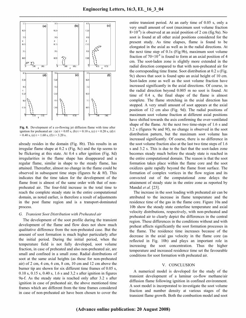
already resides in the domain (Fig. 8b). This results in an irregular flame shape at 0.2 s (Fig. 8c) and the tip seems to be flickering at this state. At 0.4 s after ignition (Fig. 8d) irregularities in the flame shape has disappeared and a regular flame, similar in shape to the steady flame, has attained. Thereafter, almost no change in the flame could be observed in subsequent time steps (figures 8e & 8f). This indicates that the time taken for the development of the flame front is almost of the same order with that of non-preheated air. The four-fold increase in the total time to reach the complete steady state in the entire computational domain, as noted earlier, is therefore a result of adjustments in the post flame region and is a transport-dominated process.

G. Transient Soot Distribution with Preheated air The development of the soot profile during the transient

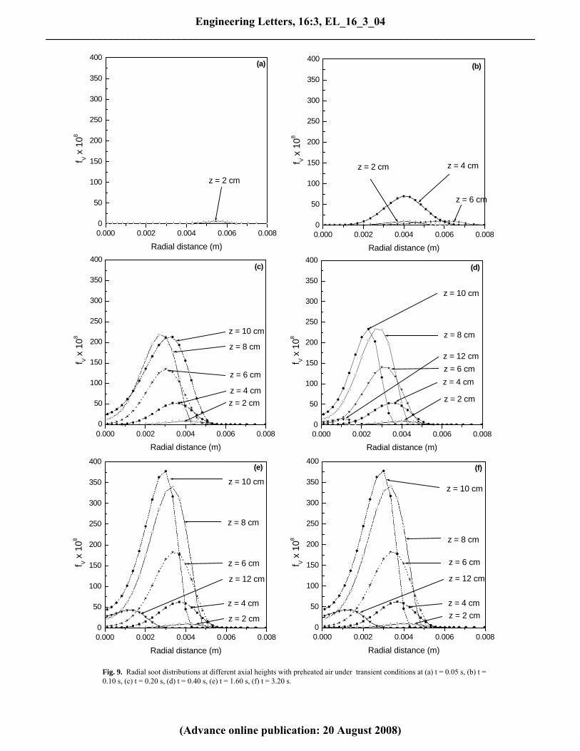
development of the flame and flow does not show much qualitative difference from the non-preheated case. But the amount of soot formation is much higher particularly after the initial period. During the initial period, when the temperature field is not fully developed, soot volume fraction, in case of preheated and also non-preheated air, are small and confined in a small zone. Radial distributions of soot at the same axial heights (as those for non-preheated air) of 2 cm, 4 cm, 6 cm, 8 cm, 10 cm and 12 cm above the burner tip are shown for six different time frames of 0.05 s, 0.10 s, 0.15 s, 0.40 s, 1.6 s and 3,2 s after ignition in figures 9a-f. As the steady state is reached only after 3.2 s after ignition in case of preheated air, the above mentioned time frames which are different from the time frames considered in case of non-preheated air have been chosen to cover the

entire transient period. At an early time of 0.05 s, only a very small amount of soot (maximum soot volume fraction 8×10-8) is observed at an axial position of 2 cm (fig.9a). No soot is found at all other axial positions considered for the present study. As time elapses, flame is found to be elongated in the axial as well as in the radial directions. At the next time step of 0.1s (Fig.9b), maximum soot volume fraction of 70×10-8 is found to form at an axial position of 4 cm. The soot-laden zone is slightly more extended in the radial direction compared to that with non-preheated air for the corresponding time frame. Soot distribution at 0.2 s (Fig. 9c) shows that soot is found upto an axial height of 10 cm. Soot-laden zone as well as the soot volume fraction have increased significantly in the axial directions. Of course, in the radial direction beyond 0.005 m no soot is found. At time of 0.4 s, the final shape of the flame is almost complete. The flame stretching in the axial direction has stopped. A very small amount of soot appears at the axial position of 12 cm also (Fig. 9d). The radial positions of maximum soot volume fraction at different axial positions have shifted towards the axis confirming the over-ventilated shape of the flame. At the next two time-steps of 1.6 s and 3.2 s (figures 9e and 9f), no change is observed in the soot distribution pattern, but the maximum soot volume has increased significantly. Of course, there is no difference in the soot volume fraction also at the last two time steps of 1.6 s and 3.2 s. This is due to the fact that the soot-laden zone becomes steady much before the steady state is reached in the entire computational domain. The reason is that the soot formation takes place within the flame core and the soot oxidizes quite rapidly beyond the flame front surface. The formation of complex vortices in the flow region and its convected out of the computational zone delays the attainment of steady state in the entire zone as reported by Mandal et al. [23].

The increase in the soot loading with preheated air can be attributed to the increase in flame temperature and the residence time of the gas in the flame core. Figure 10a and 10b show the steady state centerline temperature and axial velocity distributions, respectively, with non-preheated and preheated air to clearly depict the differences in the central region. These differences in the conditions without and with preheat affects significantly the soot formation processes in the flame. The residence time increases because of the decrease in the axial gas velocity in the flame core (as reflected in Fig. 10b) and plays an important role in increasing the soot concentration. Thus the higher temperature and increased residence time set the favourable conditions for soot formation with preheated air.

(a) (b) (c)

(d) (e) (f)

Fig. 8. Development of a co-flowing jet diffusion flame with time afterignition for preheated air : (a) t = 0.05 s, (b) t = 0.10 s, (c) t = 0.20 s, (d) t= 0.40 s, (e) t = 1.60 s, (f) t = 3.20 s.

V. CONCLUSION A numerical model is developed for the study of the

transient development of a laminar co-flow methane/air diffusion flame following ignition in confined environment. A soot model is incorporated to investigate the soot volume fraction and number density at various stages of the transient flame growth. Both the combustion model and soot



0.000 0.002 0.004 0.006 0.0080

50

100

150

200

250

300

350

400(b)

z = 6 cm

z = 4 cmz = 2 cm

f V x 1

08

Radial distance (m)

0.000 0.002 0.004 0.006 0.0080

50

100

150

200

250

300

350

400(a)

z = 2 cm

f V x 1

08

Radial distance (m)

0.000 0.002 0.004 0.006 0.0080

50

100

150

200

250

300

350

400(c)

z = 10 cm

z = 8 cm

z = 6 cm

z = 4 cmz = 2 cm

f V x 1

08

Radial distance (m)

0.000 0.002 0.004 0.006 0.0080

50

100

150

200

250

300

350

400(d)

z = 12 cm

z = 10 cm

z = 8 cm

z = 6 cmz = 4 cm

z = 2 cm

f V x 1

08

Radial distance (m)

0.000 0.002 0.004 0.006 0.0080

50

100

150

200

250

300

350

400(e)

z = 10 cm

z = 8 cm

z = 6 cm

z = 12 cm

z = 4 cm

z = 2 cm

f V x 1

08

Radial distance (m)

0.000 0.002 0.004 0.006 0.0080

50

100

150

200

250

300

350

400(f)

z = 12 cm

z = 10 cm

z = 8 cm

z = 6 cm

z = 4 cmz = 2 cm

f V x 1

08

Radial distance (m)

Fig. 9. Radial soot distributions at different axial heights with preheated air under transient conditions at (a) t = 0.05 s, (b) t = 0.10 s, (c) t = 0.20 s, (d) t = 0.40 s, (e) t = 1.60 s, (f) t = 3.20 s.



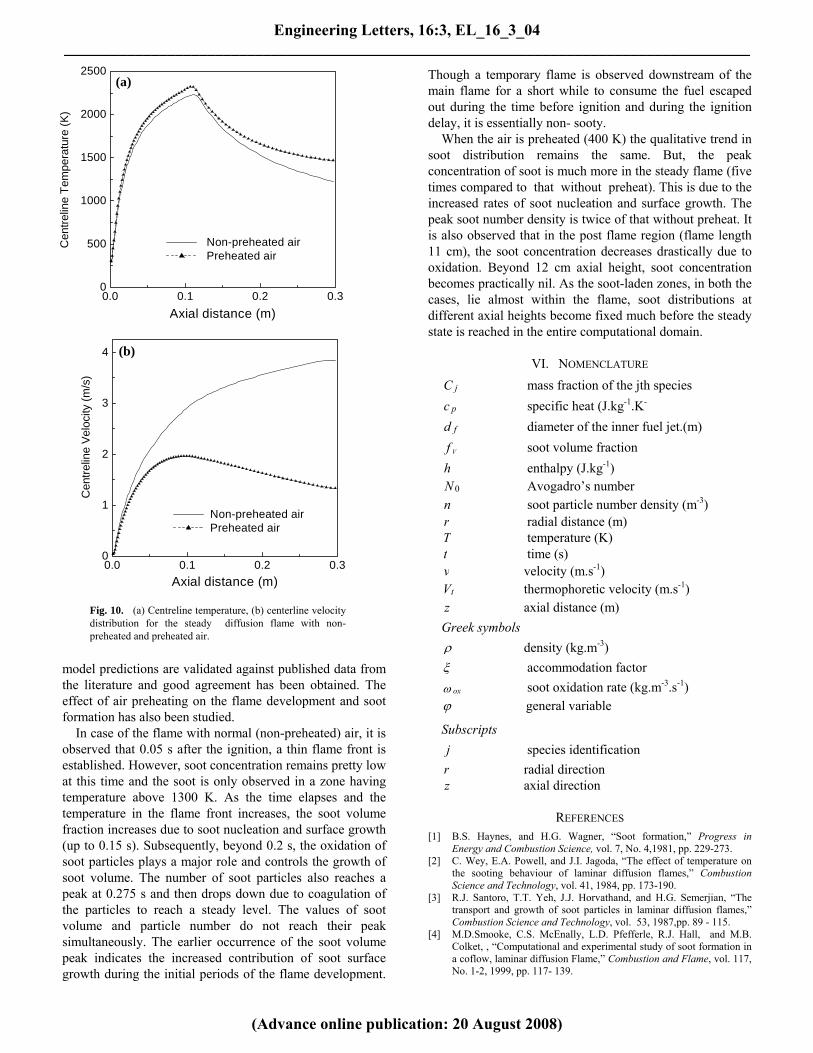
model predictions are validated against published data from the literature and good agreement has been obtained. The effect of air preheating on the flame development and soot formation has also been studied.

In case of the flame with normal (non-preheated) air, it is observed that 0.05 s after the ignition, a thin flame front is established. However, soot concentration remains pretty low at this time and the soot is only observed in a zone having temperature above 1300 K. As the time elapses and the temperature in the flame front increases, the soot volume fraction increases due to soot nucleation and surface growth (up to 0.15 s). Subsequently, beyond 0.2 s, the oxidation of soot particles plays a major role and controls the growth of soot volume. The number of soot particles also reaches a peak at 0.275 s and then drops down due to coagulation of the particles to reach a steady level. The values of soot volume and particle number do not reach their peak simultaneously. The earlier occurrence of the soot volume peak indicates the increased contribution of soot surface growth during the initial periods of the flame development.

Though a temporary flame is observed downstream of the main flame for a short while to consume the fuel escaped out during the time before ignition and during the ignition delay, it is essentially non- sooty.

0.0 0.1 0.2 0.30

500

1000

1500

2000

2500

Non-preheated air Preheated air

Cen

trelin

e Te

mpe

ratu

re (K

)

Axial distance (m)

(a)

When the air is preheated (400 K) the qualitative trend in soot distribution remains the same. But, the peak concentration of soot is much more in the steady flame (five times compared to that without preheat). This is due to the increased rates of soot nucleation and surface growth. The peak soot number density is twice of that without preheat. It is also observed that in the post flame region (flame length 11 cm), the soot concentration decreases drastically due to oxidation. Beyond 12 cm axial height, soot concentration becomes practically nil. As the soot-laden zones, in both the cases, lie almost within the flame, soot distributions at different axial heights become fixed much before the steady state is reached in the entire computational domain.

0.0 0.1 0.2 0.30

1

2

3

4

Cen

trelin

e Ve

loci

ty (m

/s)

Axial distance (m)

Non-preheated air Preheated air

(b) VI. NOMENCLATURE

jC mass fraction of the jth species

pc specific heat (J.kg-1.K-

fd diameter of the inner fuel jet.(m)

Vf soot volume fraction h enthalpy (J.kg-1)

0N Avogadro’s number n soot particle number density (m-3) r radial distance (m) T temperature (K) t time (s) v velocity (m.s-1)

tV thermophoretic velocity (m.s-1) z axial distance (m) Greek symbols ρ density (kg.m-3) ξ accommodation factor

oxω soot oxidation rate (kg.m-3.s-1) ϕ general variable

Subscripts j species identification r radial direction z axial direction

Fig. 10. (a) Centreline temperature, (b) centerline velocitydistribution for the steady diffusion flame with non-preheated and preheated air.

REFERENCES [1] B.S. Haynes, and H.G. Wagner, “Soot formation,” Progress in

Energy and Combustion Science, vol. 7, No. 4,1981, pp. 229-273. [2] C. Wey, E.A. Powell, and J.I. Jagoda, “The effect of temperature on

the sooting behaviour of laminar diffusion flames,” Combustion Science and Technology, vol. 41, 1984, pp. 173-190.

[3] R.J. Santoro, T.T. Yeh, J.J. Horvathand, and H.G. Semerjian, “The transport and growth of soot particles in laminar diffusion flames,” Combustion Science and Technology, vol. 53, 1987,pp. 89 - 115.

[4] M.D.Smooke, C.S. McEnally, L.D. Pfefferle, R.J. Hall, and M.B. Colket, , “Computational and experimental study of soot formation in a coflow, laminar diffusion Flame,” Combustion and Flame, vol. 117, No. 1-2, 1999, pp. 117- 139.



[5] K.O. Lee, C.M. Megaridis, S. Zelepouga, A.V. Saveliev, L.A. Kennedy, O. Charon, and F. Ammouri, “Soot formation effects of oxygen concentration in the oxidizer stream of laminar co-annulur non-premixed methane/air flames,” Combustion and Flame, vol. 121, No. 1-2, 2000, pp. 323 - 333.

[6] F. Xu, A.M. El-Leathy, C.H. Kin, and G.M. Faeth, “Soot surface oxidation in hydrocarbon/air diffusion flames at atmospheric pressure,” Combustion and Flame, vol. 132, No. 1-2, 2003, pp. 43 - 57.

[7] G.M. Smith, “A simple nucleation/depletion model for the spherule size of particulate carbon,” Combustion and Flame, vol. 48, 1982, pp. 265 - 272.

[8] J.P. Gore, and G.M. Faeth, Proceedings of the Combustion Institute, vol. 21, 1986, pp. 1521-1531.

[9] I.M. Kennedy, W. Kollmann, and J.Y. Chen, “A model for the soot formation in laminar diffusion flame,” Combustion and Flame, vol. 81, No. 1, 1990, pp. 73 - 85.

[10] K.M Leung, R.P. Lindstedt, and W.P. Jones, “A simplified reaction mechanism for soot formation in non-premixed flames,” Combustion and Flame, vol. 87, No. 3-4, 1991, pp. 289 - 305.

[11] R. Said, A. Garo, and R, Borghi, “Soot formation modeling for turbulent flames,” Combustion and Flame, vol. 108, No. 1-2, 1997, pp. 71 - 86.

[12] K.J. Syed, C.D. Stewart, and J.B. Moss, “.Modelling soot formation and thermal radiation in buoyant turbulent diffusion flames,” Proceedings Combustion Institute, vol. 23, 1990, pp. 1533-1539.

[13] J.B. Moss, C.D. Stewart, and K.J.Young, “Modelling soot formation and burnout in a high temperature laminar diffusion flame burning under oxygen-enriched conditions,” Combustion and Flame, vol. 101, No. 4, 1995, pp. 491 - 500.

[14] K.B. Lee, M.W. Thring, and J.M. Beer, “On the rate of combustion of soot in a laminar soot flame,” Combustion and Flame, vol. 6, 1962, pp. 137 - 145.

[15] J. Nagle, and R.F. Strickland-Constable, Fifth Carbon Conf., Vol. 1, 1962, pp. 154-164.

[16] Y.S.H. Najjar, and E.M.Goodger, “Soot oxidation in gas turbines using heavy fuels,” Fuel, vol. 60, No. 10, 1981, pp. 987 - 990.

[17] S. Mitarai, G. Kosaly, and J.J. Riley, “ A new Lagrangian flamelet model for local flame extinction and reignition,” Combustion & Flame, vol. 137, 2004, pp. 306-319.

[18] P. Sripakagorn, G. Kosaly, and J.J. Riley, “Investigation of the influence of Reynolds number on extinction and reignition,” Combustion and Flame, vol. 136, 2004, pp. 351-363.

[19] R.K. Mohammed, M.A. Tanoff, M.D. Smooke, A.M. Schaffer, and M.B. Long, , “Computational and Experimental Study of a Forced, Time-Varying, Axi-symmetric, Laminar Diffusion Flame,” Proceedings of Twenty-seventh Symp. (Int.) on Combustion, The Combustion Institute, 1998, pp. 693-702.

[20] X.L. Zhu, and J.P. Gore, “Radiation effects on combustion and pollutant emissions of high pressure opposed flow methane/air diffusion flames,” Combustion and Flame, vol. 141, 2005, pp. 118-130.

[21] Y.R. Sivathanu, and J.P. Gore, “Effects of gas-band radiation on soot kinetics in laminar methane/air diffusion flames,”, Combustion and Flame, vol. 110, 1997, pp. 256-263.

[22] E. Mastorakas, A.M.K.P.Tayor, and J.H . Whitelaw, “Extinction of Turbulent Counterflow Flames with Reactants Diluted by Hot Products,” Combustion and Flame, vol. 102,1995, pp. 101-114.

[23] B.K. Mandal, A. Datta, and A. Sarkar,“Transient development of methane-air diffusion flame in a confined geometry with and without air-preheat,” International Journal for Energy Research, vol. 29, No. 2, 2005, pp. 145-176.

[24] J.B. Heywood, Internal Combustion Engine Fundamentals, McGraw-Hill. 1989, New York. USA.

[25] C.W. Hirt, and J.L. Cook, “Calculating three-dimensional flows around structures and over rough terrain,” Journal of Computational Physics, vol. 10, 1972, pp. 324 – 338.

[26] A. Datta, “Effects of variable property formulation on the prediction of a CH4-Air laminar jet diffusion flame,” Proceedings of 6th

ISHMT/ASME Heat and Mass Transfer Conference, India, 2004, pp. 532-540.

[27] R.E. Mitchell, A.F. Sarofim, and L.A. Clomburg, “Experimental and numerical investigation of confined laminar diffusion flames,” Combustion and Flame, vol. 3, 1980, pp. 227 -244.

[28] C.W. Hirt, B.D. Nickols, and N.C. Romero, SOLA – A Numerical Solution Algorithm for Transient Fluid Flows, Los Alamos Scientific Laboratory Report, 1975, LA – 5852, Los Alamos, New Mexico.



Documents

A Computational Study of the Soot Formation in Methane-Air … · A Computational Study of the Soot Formation in Methane-Air Diffusion Flame During Early Transience Following Ignition