University of Texas at El PasoDigitalCommons@UTEP

Open Access Theses & Dissertations

2016-01-01

Computational Modeling of a 60kW Oxy-MethaneDirect Power Extraction CombustorOmar Daniel VidanaUniversity of Texas at El Paso, odvidana@miners.utep.edu

Follow this and additional works at: https://digitalcommons.utep.edu/open_etdPart of the Aerospace Engineering Commons, Mechanical Engineering Commons, and the Oil,

Gas, and Energy Commons

This is brought to you for free and open access by DigitalCommons@UTEP. It has been accepted for inclusion in Open Access Theses & Dissertationsby an authorized administrator of DigitalCommons@UTEP. For more information, please contact lweber@utep.edu.

Recommended CitationVidana, Omar Daniel, "Computational Modeling of a 60kW Oxy-Methane Direct Power Extraction Combustor" (2016). Open AccessTheses & Dissertations. 979.https://digitalcommons.utep.edu/open_etd/979

COMPUTATIONAL MODELING OF A 60KW OXY-METHANE DIRECT

POWER EXTRACTION COMBUSTOR

OMAR DANIEL VIDAÑA

Master’s Program in Mechanical Engineering

APPROVED:

Norman Love, Ph.D., Chair

Yirong Lin, Ph.D.

Bill Tseng, Ph.D.

Charles Amber, Ph.D.

Dean of the Graduate School

Copyright ©

by

Omar D. Vidaña

2016

Dedication

I dedicate this thesis to my mother. I’m here because of your support and sacrifices, gracias

mama! Thanks also to Dr. Norman Love, for giving me the opportunity to acquire engineering

experience that I will carry on for the rest of my life.

COMPUTATIONAL MODELING OF A 60KW OXY-METHANE DIRECT

POWER EXTRACTION COMBUSTOR

by

OMAR DANIEL VIDAÑA, B.S.M.E.

THESIS

Presented to the Faculty of the Graduate School of

The University of Texas at El Paso

in Partial Fulfillment

of the Requirements

for the Degree of

MASTER OF SCIENCE

Master’s Program in Mechanical Engineering

THE UNIVERSITY OF TEXAS AT EL PASO

August, 2016

v

Acknowledgements

The research is supported by the US Department of Energy, under award DE-FE-0024062

(Project Manager Jason Hissam). However, any opinions, findings, conclusions, or

recommendations expressed herein are those of the authors and do not necessarily reflect the views

of the Department of Energy.

vi

Table of Contents

Acknowledgements ..........................................................................................................................v

Table of Contents ........................................................................................................................... vi

List of Tables ............................................................................................................................... viii

List of Figures ................................................................................................................................ ix

Chapter 1: Introduction and Background .........................................................................................1

1.1 Overview ........................................................................................................................1

1.2 Magnetohydroynamic Power Generators ......................................................................2

1.3 Faraday’s Principle ........................................................................................................3

1.4 Previous Work ...............................................................................................................4

Chapter 2: Theory ............................................................................................................................7

2.1 Fundamental Equations ..................................................................................................7

2.2 Mesh .............................................................................................................................19

2.3 Boundary Conditions ...................................................................................................21

Chapter 3: Results and Discussion .................................................................................................25

3.1 Swirl Coaxial Injector ..................................................................................................25

3.2 Converging-Diverging Nozzle .....................................................................................29

3.3 Cooling System ............................................................................................................36

Chapter 4: Summary and Conclusions ...........................................................................................38

References ......................................................................................................................................40

Appendix A: Sample Calculations .................................................................................................42

Fuel & Oxidizer Mass Flow Rates ........................................................................................42

Throat Conditions .................................................................................................................43

Cooling System Pump Optimal Flow Rate ...........................................................................45

CEA Results ..........................................................................................................................49

Appendix B: CADs and Schematics ..............................................................................................51

DPE Combustor Assembly ...................................................................................................51

DPE Combustor Exploded View ..........................................................................................52

DPE Combustor ....................................................................................................................53

vii

Cooling Jacket .......................................................................................................................54

Fuel Manifold........................................................................................................................55

Water Line Schematic ...........................................................................................................56

Vita ...............................................................................................................................................57

viii

List of Tables

Table 1: Enthalpy Extraction Percentages ...................................................................................... 5 Table 2: Governing equations variables ......................................................................................... 8 Table 3: Injector pressure drop variables ...................................................................................... 10 Table 4: Non-premixed model variables....................................................................................... 13 Table 5: Combined stress & Sieder-Tate equation variables ........................................................ 16

Table 6: Cooling system model variables ..................................................................................... 18 Table 7: Boundary conditions for the swirl coaxial injector ......................................................... 22 Table 8: Boundary conditions for the converging-diverging nozzle ............................................ 23 Table 9: Boundary conditions for the cooling system .................................................................. 24 Table 10: Results comparison between CEA and Fluent model .................................................. 29

Table 11: Flow rate calculation variables ..................................................................................... 43 Table 12: Heat flux calculation values .......................................................................................... 44

Table 13: Combined stress calculation values .............................................................................. 44 Table 14: Componets pressure drop ............................................................................................. 45

Table 15: Sudden expanison, sudden contraciton and bends pressure drop ................................. 46 Table 16: Pressure drop along the pipes ....................................................................................... 46

Table 17: Head loss and ΔP at various flow rates......................................................................... 47

ix

List of Figures

Figure 1: Turbogenerator vs. MHD generator ................................................................................ 2 Figure 2: Gas conductivity vs. Ionization for open cycle MHD generators ................................... 3 Figure 3: Fleming’s Right Hand Rule ............................................................................................. 4 Figure 4: DPE combustor drawing ................................................................................................. 7 Figure 5: Swirl coaxial injector....................................................................................................... 9

Figure 6: Early swirl coaxial injector with ring manifold ............................................................. 11 Figure 7: DPE combustor and converging-diverging nozzle ........................................................ 12 Figure 8: : Simplified DPE combustor.......................................................................................... 14 Figure 9: DPE combustor concept ................................................................................................ 15 Figure 10: Cooling channels ......................................................................................................... 16

Figure 11: Cooling Jacket ............................................................................................................. 17 Figure 12: Simplified cooling system model ................................................................................ 19

Figure 13: Swirl coaxial injector mesh ......................................................................................... 20 Figure 14: Combustor and converging-diverging nozzle mesh .................................................... 20

Figure 15: Cooling system mesh................................................................................................... 21 Figure 16: Fuel injector static pressure controur, units shown are in kPa .................................... 25

Figure 17: Fuel injector velocity contour, units shown in m/s ..................................................... 26 Figure 18(a): Injector volume fraction contour of methane at 0.1 ms .......................................... 26 Figure 18(b): Injector volume fraction contour of methane at 0.5 ms .......................................... 26

Figure 18(c): Injector volume fraction contour of methane at 1 ms ............................................. 27 Figure 18(d): Injector volume fraction contour of methane at 2 ms ............................................. 27

Figure 18(e): Injector volume fraction contour of methane at 4.45 ms ........................................ 27

Figure 19: Early fuel injector static pressure controur, units shown are in kPa ........................... 28

Figure 20: Early fuel injector velocity contour, units shown are in m/s ....................................... 28 Figure 21: Early injector volume fraction contours of methane at 1 and 3 ms ............................. 29

Figure 22: Velocity contour with combustion, units shown are in m/s ........................................ 30 Figure 23: Temperature contour with combustion, units shown are in K .................................... 30 Figure 24: Methane velocity vectors............................................................................................. 31

Figure 25: Methane pathlines........................................................................................................ 32 Figure 26: Oxygen pathlines ......................................................................................................... 32

Figure 27: Converging-diverging nozzle boundary layer ............................................................. 33 Figure 28: Simplified combustor velocity contour, units shown are in m/s ................................. 34 Figure 29: Simplified combustor temperature contour, units shown are in K .............................. 34 Figure 30: Simplified combustor methane velocity vectors ......................................................... 35

Figure 31: Simplified combustor methane pathlines .................................................................... 35

Figure 32: Simplified combustor oxygen pathlines ...................................................................... 36

Figure 33: Temperature contour for the cooling system, units shown are in K ............................ 37 Figure 34: Simplified cooling system pressure contour ............................................................... 37 Figure 35: DPE combustor............................................................................................................ 39 Figure 36: Sudden contractions loss coefficient chart .................................................................. 45 Figure 37: Pump performance curve vs. System curve ................................................................ 48

1

Chapter 1: Introduction and Background

1.1 OVERVIEW

Recently, the demand for alternative sources of energy has increased. This is partially due

to the effects observed over many years of burning coal and other fossil fuels to generate

electricity. The main disadvantage of burning coal and fossil fuels is the amount of carbon dioxide

produced. Coal and fossil fuels were responsible for 31% of the 6,673 million metric tons of carbon

dioxide emitted in United States in 20131. Although carbon dioxide is a primary pollutant, power

generation produces other contaminants as well. For instance, power generation alone contributes

to approximately 70% of SO2, 20% of NOx, and 40% of mercury emissions2. These emissions do

not only cause health problems to humans but also to the environment. The pollutant residence

time is a key factor that must be considered when assessing the damage to the environment. This

time may vary from few days to several years. When pollutants eventually fall back to the ground

they can return in various forms such as rain, snow, fog, gases or particles2. More detailed effects

can arise. For SO2 and NOx, these interact with the atmosphere to form acidic mixtures, small

particles and ozone2. Acidic rain lowers the pH of lakes and rivers adversely affecting the health

of the living organisms that depend on them. The small particles formed by SO2 and NOx decrease

visibility and may cause severe respiratory problems in humans. Furthermore, NOx emissions react

in the presence of sunlight to form ozone which is a major component of smog2. Finally, mercury

may be deposited in water bodies and consumed by fish, fish-eating birds and mammals2. Humans

can then accidentally eat these contaminated animals and after a prolonged exposure suffer

neurological damage.

One of the dominant types of power generation systems used today are gas turbines. Over

the years, gas turbines have been an incredible source of reliability, efficiency, and have evolved

to operate at temperatures as high as 2000K3. To counteract the high levels of toxic emissions in

the earth’s atmosphere carbon capture techniques have been considered. Oxy-combustion is a

2

carbon capture technique that uses oxygen instead of air when burning a hydrocarbon fuel. The

advantage of an oxy-combustion system is that the products are carbon dioxide and steam, from

which the steam can be condensed and the carbon dioxide sequestered meaning little to no

emissions. However, flame temperature for an oxy-combustion system can exceed 3000K, which

is well above current material operability limits of the combustor and gas turbine systems in use.

To reduce flame temperature, fuel inlets are typically mixed with recycled carbon dioxide or other

diluents, which results in overall lower temperature and system efficiency. In order to efficiently

use oxy-combustion systems it is desired to operate at these high temperatures.

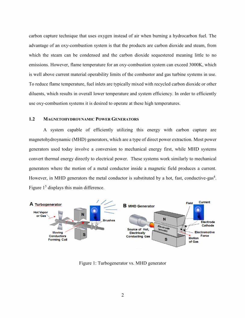
1.2 MAGNETOHYDROYNAMIC POWER GENERATORS

A system capable of efficiently utilizing this energy with carbon capture are

magnetohydroynamic (MHD) generators, which are a type of direct power extraction. Most power

generators used today involve a conversion to mechanical energy first, while MHD systems

convert thermal energy directly to electrical power. These systems work similarly to mechanical

generators where the motion of a metal conductor inside a magnetic field produces a current.

However, in MHD generators the metal conductor is substituted by a hot, fast, conductive-gas4.

Figure 15 displays this main difference.

Figure 1: Turbogenerator vs. MHD generator

3

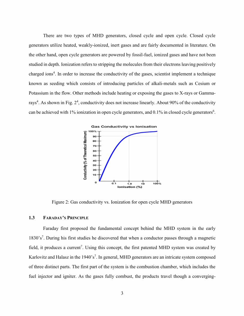
There are two types of MHD generators, closed cycle and open cycle. Closed cycle

generators utilize heated, weakly-ionized, inert gases and are fairly documented in literature. On

the other hand, open cycle generators are powered by fossil-fuel, ionized gases and have not been

studied in depth. Ionization refers to stripping the molecules from their electrons leaving positively

charged ions4. In order to increase the conductivity of the gases, scientist implement a technique

known as seeding which consists of introducing particles of alkali-metals such as Cesium or

Potassium in the flow. Other methods include heating or exposing the gases to X-rays or Gamma-

rays4. As shown in Fig. 24, conductivity does not increase linearly. About 90% of the conductivity

can be achieved with 1% ionization in open cycle generators, and 0.1% in closed cycle generators6.

Figure 2: Gas conductivity vs. Ionization for open cycle MHD generators

1.3 FARADAY’S PRINCIPLE

Faraday first proposed the fundamental concept behind the MHD system in the early

1830’s7. During his first studies he discovered that when a conductor passes through a magnetic

field, it produces a current7. Using this concept, the first patented MHD system was created by

Karlovitz and Halasz in the 1940’s7. In general, MHD generators are an intricate system composed

of three distinct parts. The first part of the system is the combustion chamber, which includes the

fuel injector and igniter. As the gases fully combust, the products travel though a converging-

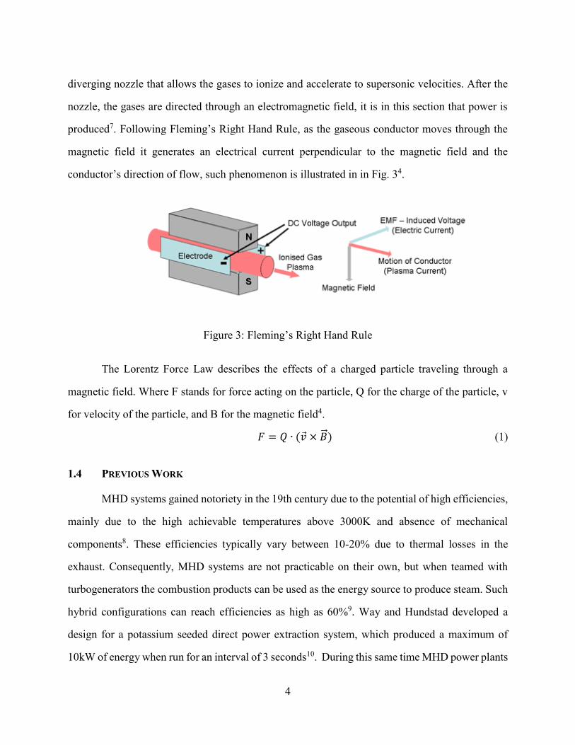
4

diverging nozzle that allows the gases to ionize and accelerate to supersonic velocities. After the

nozzle, the gases are directed through an electromagnetic field, it is in this section that power is

produced7. Following Fleming’s Right Hand Rule, as the gaseous conductor moves through the

magnetic field it generates an electrical current perpendicular to the magnetic field and the

conductor’s direction of flow, such phenomenon is illustrated in in Fig. 34.

Figure 3: Fleming’s Right Hand Rule

The Lorentz Force Law describes the effects of a charged particle traveling through a

magnetic field. Where F stands for force acting on the particle, Q for the charge of the particle, v

for velocity of the particle, and B for the magnetic field4.

𝐹 = 𝑄 ∙ (�� × ��) (1)

1.4 PREVIOUS WORK

MHD systems gained notoriety in the 19th century due to the potential of high efficiencies,

mainly due to the high achievable temperatures above 3000K and absence of mechanical

components8. These efficiencies typically vary between 10-20% due to thermal losses in the

exhaust. Consequently, MHD systems are not practicable on their own, but when teamed with

turbogenerators the combustion products can be used as the energy source to produce steam. Such

hybrid configurations can reach efficiencies as high as 60%9. Way and Hundstad developed a

design for a potassium seeded direct power extraction system, which produced a maximum of

10kW of energy when run for an interval of 3 seconds10. During this same time MHD power plants

5

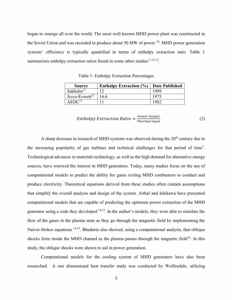
began to emerge all over the world. The most well-known MHD power plant was constructed in

the Soviet Union and was recorded to produce about 50 MW of power 10. MHD power generation

systems’ efficiency is typically quantified in terms of enthalpy extraction ratio. Table 1

summarizes enthalpy extraction ratios found in some other studies11,12,13.

Table 1: Enthalpy Extraction Percentages

Source Enthalpy Extraction (%) Date Published

Sakhalin11 12 1999

Avco-Everett12 16.6 1975

AEDC13 11 1982

𝐸𝑛𝑡ℎ𝑎𝑙𝑝𝑦 𝐸𝑥𝑡𝑟𝑎𝑐𝑡𝑖𝑜𝑛 𝑅𝑎𝑡𝑖𝑜 =𝑃𝑜𝑤𝑒𝑟 𝑂𝑢𝑡𝑝𝑢𝑡

𝑇ℎ𝑒𝑟𝑚𝑎𝑙 𝐼𝑛𝑝𝑢𝑡 (2)

A sharp decrease in research of MHD systems was observed during the 20th century due to

the increasing popularity of gas turbines and technical challenges for that period of time7.

Technological advances in materials technology, as well as the high demand for alternative energy

sources, have renewed the interest in MHD generators. Today, many studies focus on the use of

computational models to predict the ability for gases exiting MHD combustors to conduct and

produce electricity. Theoretical equations derived from these studies often contain assumptions

that simplify the overall analysis and design of the system. Aithal and Ishikawa have presented

computational models that are capable of predicting the optimum power extraction of the MHD

generator using a code they developed 14,15. In the author’s models, they were able to simulate the

flow of the gases in the plasma state as they go through the magnetic field by implementing the

Naiver-Stokes equations 14,15. Bhadoria also showed, using a computational analysis, that oblique

shocks form inside the MHD channel as the plasma passes through the magnetic field16. In this

study, the oblique shocks were shown to aid in power generation.

Computational models for the cooling system of MHD generators have also been

researched. A one dimensional heat transfer study was conducted by Wolfendale, utilizing

6

OpenFoam to model the fusion blanket in an MHD generator17. With this code the authors were

able to predict the pressure loss and temperature profiles along the combustor walls. Combustion

processes have also been simulated using the commercial software ANSYS-CFX to aid in the

design of a rocket engine18. The combustion model proposed incorporates the Eddy-Dissipation

models for oxygen-hydrogen combustion18. Utilizing this tool, the authors showed how the initial

design was modified so that an adequate temperature profile could be obtained in the engine17.

Although some studies are available on the topic, overall there is a lack of research of

computational models for the design of the combustion chamber, cooling unit, and nozzle section

of open cycle MHD systems. Motivated by this, this paper aims to contribute to the current body

of knowledge by presenting the computational models used in the design of an MHD combustor,

conical converging diverging nozzle, and cooling system for a small-scale open-cycle MHD

generator that operates using gaseous methane and oxygen.

7

Chapter 2: Theory

2.1 FUNDAMENTAL EQUATIONS

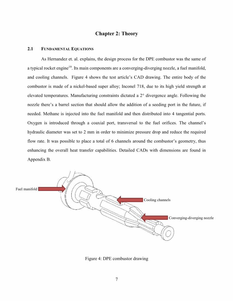
As Hernandez et. al. explains, the design process for the DPE combustor was the same of

a typical rocket engine19. Its main components are a converging-diverging nozzle, a fuel manifold,

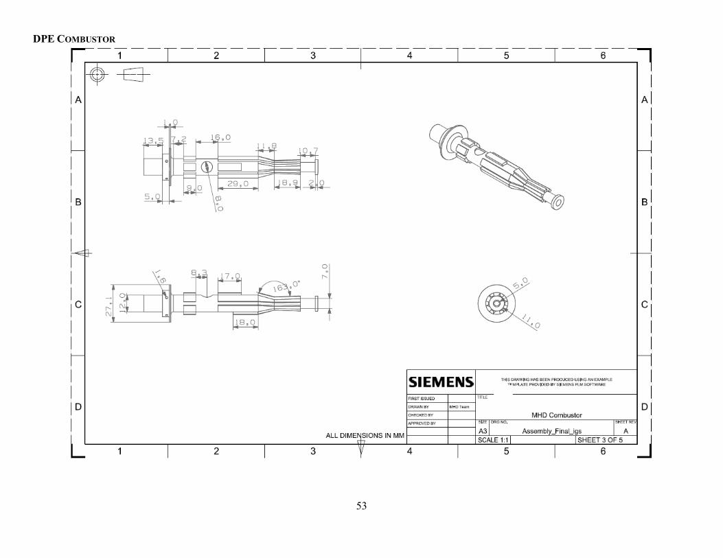
and cooling channels. Figure 4 shows the test article’s CAD drawing. The entire body of the

combustor is made of a nickel-based super alloy; Inconel 718, due to its high yield strength at

elevated temperatures. Manufacturing constraints dictated a 2° divergence angle. Following the

nozzle there’s a barrel section that should allow the addition of a seeding port in the future, if

needed. Methane is injected into the fuel manifold and then distributed into 4 tangential ports.

Oxygen is introduced through a coaxial port, transversal to the fuel orifices. The channel’s

hydraulic diameter was set to 2 mm in order to minimize pressure drop and reduce the required

flow rate. It was possible to place a total of 6 channels around the combustor’s geometry, thus

enhancing the overall heat transfer capabilities. Detailed CADs with dimensions are found in

Appendix B.

Figure 4: DPE combustor drawing

Fuel manifold

Converging-diverging nozzle

Cooling channels

8

The governing mass and momentum equations, Eqs. (3-7)20, were solved using software

package ANSYS Fluent. All components utilized the mass and momentum equations hence they

are presented first. Boundary conditions and details of the solving procedure for each component

shown in Fig. 4 is presented in the following sections. Governing equations pertinent to each

component are also presented in the following sections.

𝜕𝜌

𝜕𝑡+ ∇ ∙ (𝜌��) = 0 (3)

𝜕

𝜕𝑡(𝜌𝑣) + ∇ ∙ (𝜌����) = −∇𝑝 + ∇ ∙ (𝜏) + 𝜌�� + �� (4)

Where 𝜏 is the stress tensor given by Eq. (5)20.

𝜏 = 𝜇 [(∇�� + ∇��𝑇 −2

3∇ ∙ ��𝐼] (5)

The mixing and shearing flow experienced in the injector along with high expected

Reynolds numbers led to the assumption of turbulent flow. To model the turbulence, the standard

k-ε model was implemented in the solver. The k-ε model introduces two extra transport equations

for kinetic energy (k) and dissipation(𝜖), Eqs. (6,7)20. 𝜕

𝜕𝑡(𝜌𝑘) +

𝜕

𝜕𝑥𝑖(𝜌𝑘𝑢𝑖) =

𝜕

𝜕𝑥𝑗[(𝜇 +

𝜇𝑡

𝜎𝑘)

𝜕𝑘

𝜕𝑥𝑗] + 𝐺𝑘 + 𝐺𝑏 − 𝜌𝜖 − 𝑌𝑀 + 𝑆𝑘 (6)

𝜕

𝜕𝑡(𝜌𝜖) +

𝜕

𝜕𝑥𝑖(𝜌𝜖𝑢𝑖) =

𝜕

𝜕𝑥𝑗[(𝜇 +

𝜇𝑡

𝜎𝜖)

𝜕𝜖

𝜕𝑥𝑗] + 𝐶1𝜖

𝜖

𝑘(𝐺𝑘 + 𝐶3𝜖𝐺𝑏) − 𝐶2𝜖𝜌

𝜖2

𝑘− 𝑆𝜖 (7)

Table 2: Governing equations variables

Symbol Name

𝜌 Density

𝜖 Dissipation rate

𝜇 Dynamic viscosity

𝑔 Gravity

𝐺𝑏 Kinetic energy generation due to buoyancy

𝐺𝑘 Kinetic energy generation due to velocity

𝜇𝑡 Laminar viscosity

𝑌𝑀 Overall dissipation rate

𝑃 Pressure

𝜏 Stress tensor

𝑘 Turbulent kinetic energy

𝑣 Velocity

9

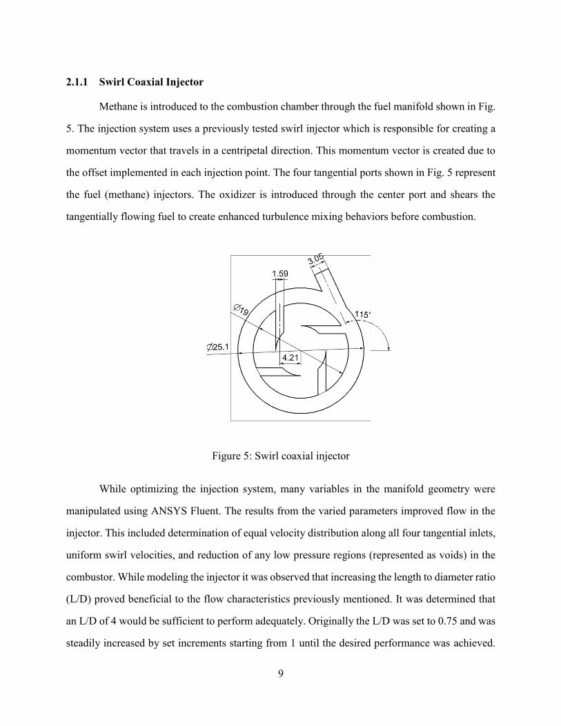
2.1.1 Swirl Coaxial Injector

Methane is introduced to the combustion chamber through the fuel manifold shown in Fig.

5. The injection system uses a previously tested swirl injector which is responsible for creating a

momentum vector that travels in a centripetal direction. This momentum vector is created due to

the offset implemented in each injection point. The four tangential ports shown in Fig. 5 represent

the fuel (methane) injectors. The oxidizer is introduced through the center port and shears the

tangentially flowing fuel to create enhanced turbulence mixing behaviors before combustion.

Figure 5: Swirl coaxial injector

While optimizing the injection system, many variables in the manifold geometry were

manipulated using ANSYS Fluent. The results from the varied parameters improved flow in the

injector. This included determination of equal velocity distribution along all four tangential inlets,

uniform swirl velocities, and reduction of any low pressure regions (represented as voids) in the

combustor. While modeling the injector it was observed that increasing the length to diameter ratio

(L/D) proved beneficial to the flow characteristics previously mentioned. It was determined that

an L/D of 4 would be sufficient to perform adequately. Originally the L/D was set to 0.75 and was

steadily increased by set increments starting from 1 until the desired performance was achieved.

10

The length of the ports was constrained by manufacturing techniques that would be used to

construct this same injector. Another variable that was analyzed was the path of injection

(clockwise or counterclockwise). It was determined that clockwise was the most efficient

configuration. Based on these observations, the final design was chosen and is shown in Fig. 5.

The manifold dimensions were initially in imperial units. Therefore, translation to the

metric system is displayed with two significant figures for better accuracy. The width of the

manifold ring is 6.1 mm; the inner diameter is 19 mm while the outer diameter is 25.1 mm. Every

orifice is 1.59 mm in diameter with an offset distance of 4.21 mm from the center. The inlet pipe

is 3.05 mm in diameter and is introduced at 115° in respect to the x-axis. Furthermore, the injector’s

310 kPa pressure drop was quantified using Eq. (8)21.

𝑞 = 𝑌𝐶𝐴√2𝑔(144)∆𝑃

𝜌 (8)

Table 3: Injector pressure drop variables

Symbol Name

𝐴 Area

𝜌 Density

𝑌 Expansion factor

𝐶 Flow coefficient

𝑔 Gravity

∆𝑃 Pressure difference

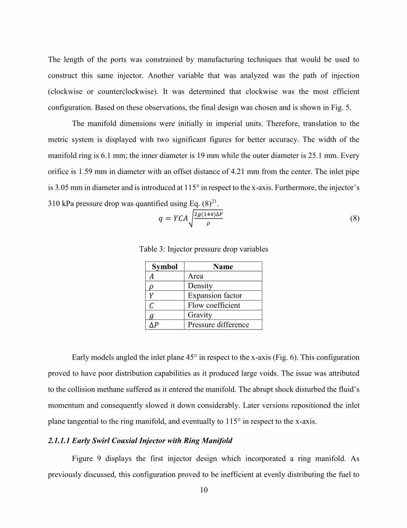
Early models angled the inlet plane 45° in respect to the x-axis (Fig. 6). This configuration

proved to have poor distribution capabilities as it produced large voids. The issue was attributed

to the collision methane suffered as it entered the manifold. The abrupt shock disturbed the fluid’s

momentum and consequently slowed it down considerably. Later versions repositioned the inlet

plane tangential to the ring manifold, and eventually to 115° in respect to the x-axis.

2.1.1.1 Early Swirl Coaxial Injector with Ring Manifold

Figure 9 displays the first injector design which incorporated a ring manifold. As

previously discussed, this configuration proved to be inefficient at evenly distributing the fuel to

11

all four tangential ports. The geometry was optimized for a combustor with much thicker walls.

Consequently, it was able to afford a longer L/D ratio. Once it was determined that the DPE

combustor would employ a 1 mm wall thickness the L/D was adapted accordingly. Other

dimensions that evolved included the ring manifold width and the inlet plane angle. A feature that

proved to be ineffective and eventually removed was a small indentation 3.24 millimeters in

diameter intended to redirect the flow of the fuel to the orifices. It was determined that the crucial

dimensions that could not be modified were the orifice diameter for the four tangential ports, and

their respective offset.

Figure 6: Early swirl coaxial injector with ring manifold

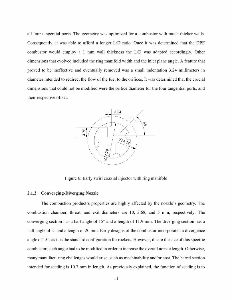
2.1.2 Converging-Diverging Nozzle

The combustion product’s properties are highly affected by the nozzle’s geometry. The

combustion chamber, throat, and exit diameters are 10, 3.68, and 5 mm, respectively. The

converging section has a half angle of 15° and a length of 11.9 mm. The diverging section has a

half angle of 2° and a length of 20 mm. Early designs of the combustor incorporated a divergence

angle of 15°, as it is the standard configuration for rockets. However, due to the size of this specific

combustor, such angle had to be modified in order to increase the overall nozzle length. Otherwise,

many manufacturing challenges would arise, such as machinability and/or cost. The barrel section

intended for seeding is 10.7 mm in length. As previously explained, the function of seeding is to

12

activate the conductivity of the weakly ionized combustion products. Figure 7 shows a cross-

sectional view of the test article.

Such dimensions, in conjunction with the DPE combustor’s operating conditions

(discussed later in this chapter) yielded an under-expanded nozzle. Thus sacrificing velocity in

order to preserve an elevated exit temperature. A conventional DPE system requires flame

temperatures between 2800–3000K to improve electrical conductivity. Furthermore, velocities of

1800 – 2000 m/s are required to increase the energy extraction potential. If the combustion

products do not meet both requirements energy extraction is not possible.

Figure 7: DPE combustor and converging-diverging nozzle

For simplicity, initial assumptions included constant chamber pressure and isentropic

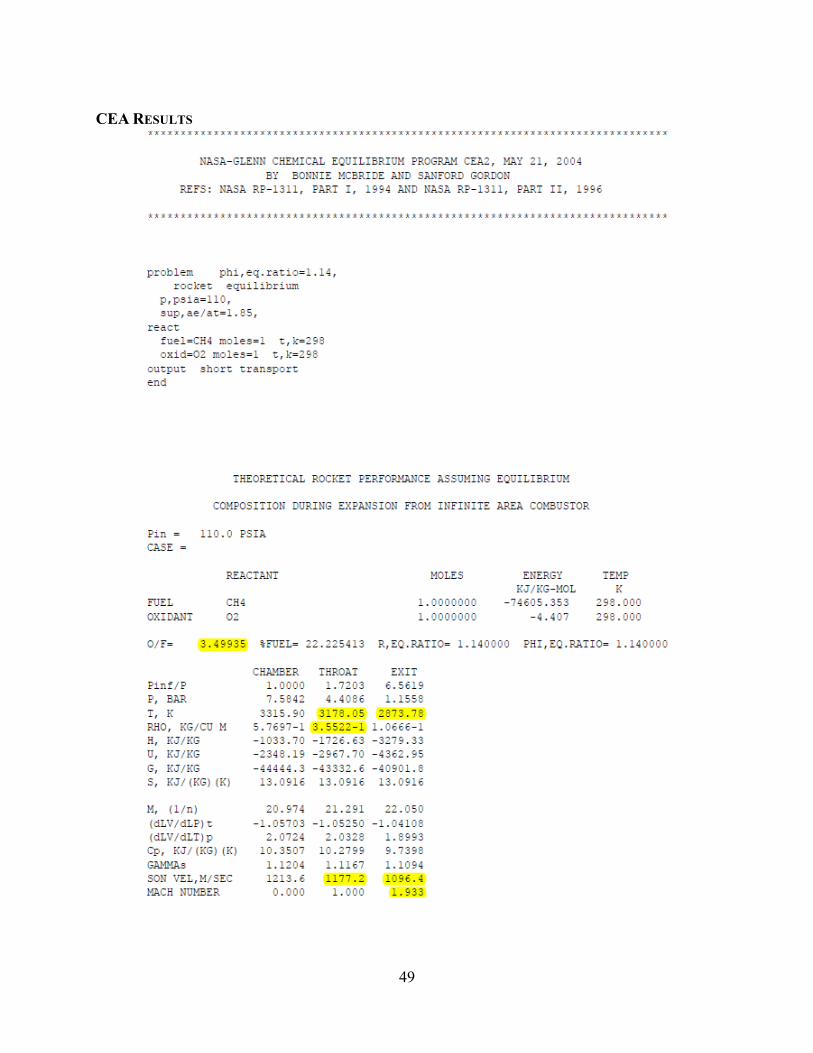
conditions. In order to obtain the exit temperature and velocity from the nozzle, NASA chemical

equilibrium with applications (CEA) software was utilized. CEA was developed by the Lewis

Research Center and is widely used for aerodynamic and thermodynamic applications. The

program obtains its information from independent databases, from which it computes chemical

reactions for any specified mixture and defines its thermodynamic and transport properties22. The

one dimensional code assisted in the determination of a baseline of expected temperatures,

products, and pressures in the system. The CEA code was run assuming an equivalence ratio of

1.14, chamber pressure of 758.42 kPa, and an exit to throat area ratio of 1.85. Combustion products

were run using the assumption of frozen equilibrium. When implementing these conditions, an

exit temperature of 2874 K and velocity of 2119 m/s were calculated. Full results can be found in

Appendix A.

13

A Fluent non-premixed combustion model was used and results compared with CEA. This

model attempts to simplify the thermochemistry to the mixture fraction. The mixture fraction,

represented by ƒ, is the mass ratio of burnt and unburnt elements23.

𝑓 =𝑍𝑖−𝑍𝑖,𝑜𝑥

𝑍𝑖,𝑓𝑢𝑒𝑙−𝑍𝑖,𝑜𝑥 (9)

By using this model species were determined from predicted mixture fraction quantities.

Moreover, the relationship between turbulence and chemistry is modeled using a Probability

Density Function (PDF). The PDF is computed before the simulation starts using the elements’

initial conditions, which for this study is one mole of methane and two moles of oxygen. By

performing these operations, the overall computational time was reduced.

For this model the fluids were assumed to have equal diffusivities, thus the species

equations were condensed to a single mixture fraction function. Due to the fact that elements are

conserved in chemical reactions, it is possible to cancel the reaction terms in the species equations.

This assumption is typically suitable for turbulent flow only, as the turbulent convection

overcomes molecular diffusion23. The Favre mean mixture fraction is denoted as: 𝜕

𝜕𝑡(𝜌𝑓

′) + ∇(𝜌��𝑓) = ∇ (

𝜇𝑙+𝜇𝑡

𝜎𝑡∇𝑓) + 𝑆𝑚 + 𝑆𝑢𝑠𝑒𝑟 (10)

Fluent solves for the conservation equation for the mixture fraction variance, which is

obtained by expanding Eq. (10)23 to: 𝜕

𝜕𝑡(𝜌𝑓′2) + ∇ (𝜌��𝑓′2) = ∇ (

𝜇𝑙+𝜇𝑡

𝜎𝑡∇𝑓′2) + 𝐶𝑔𝜇𝑡(∇𝑓)2 − 𝐶𝑑𝜌

𝜀

𝑘𝑓′2 + 𝑆𝑢𝑠𝑒𝑟 (11)

Table 4: Non-premixed model variables

Symbol Value

𝜌 Density

𝜀 Dissipation rate

𝜇𝑙 Laminar viscosity

𝑍𝑖 Mass fraction of element i

𝑍𝑓𝑢𝑒𝑙 Mass fraction of fuel

𝑍𝑜𝑥 Mass fraction of oxygen

𝑓 Mixture fraction

𝑘 Turbulent kinetic energy

𝜇𝑡 Turbulent viscosity

𝑣 Velocity

14

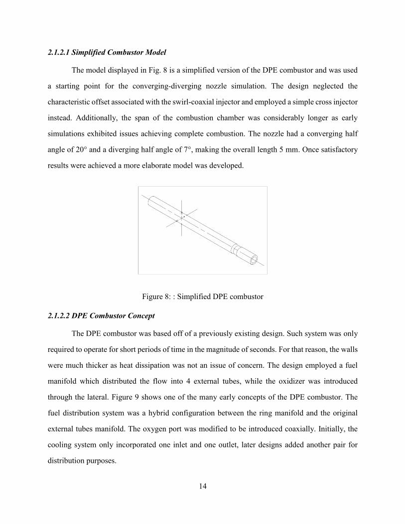
2.1.2.1 Simplified Combustor Model

The model displayed in Fig. 8 is a simplified version of the DPE combustor and was used

a starting point for the converging-diverging nozzle simulation. The design neglected the

characteristic offset associated with the swirl-coaxial injector and employed a simple cross injector

instead. Additionally, the span of the combustion chamber was considerably longer as early

simulations exhibited issues achieving complete combustion. The nozzle had a converging half

angle of 20° and a diverging half angle of 7°, making the overall length 5 mm. Once satisfactory

results were achieved a more elaborate model was developed.

Figure 8: : Simplified DPE combustor

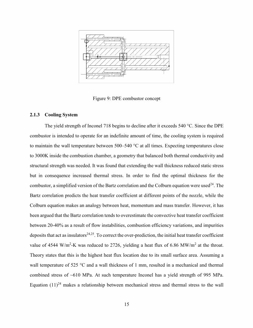
2.1.2.2 DPE Combustor Concept

The DPE combustor was based off of a previously existing design. Such system was only

required to operate for short periods of time in the magnitude of seconds. For that reason, the walls

were much thicker as heat dissipation was not an issue of concern. The design employed a fuel

manifold which distributed the flow into 4 external tubes, while the oxidizer was introduced

through the lateral. Figure 9 shows one of the many early concepts of the DPE combustor. The

fuel distribution system was a hybrid configuration between the ring manifold and the original

external tubes manifold. The oxygen port was modified to be introduced coaxially. Initially, the

cooling system only incorporated one inlet and one outlet, later designs added another pair for

distribution purposes.

15

Figure 9: DPE combustor concept

2.1.3 Cooling System

The yield strength of Inconel 718 begins to decline after it exceeds 540 °C. Since the DPE

combustor is intended to operate for an indefinite amount of time, the cooling system is required

to maintain the wall temperature between 500–540 °C at all times. Expecting temperatures close

to 3000K inside the combustion chamber, a geometry that balanced both thermal conductivity and

structural strength was needed. It was found that extending the wall thickness reduced static stress

but in consequence increased thermal stress. In order to find the optimal thickness for the

combustor, a simplified version of the Bartz correlation and the Colburn equation were used24. The

Bartz correlation predicts the heat transfer coefficient at different points of the nozzle, while the

Colburn equation makes an analogy between heat, momentum and mass transfer. However, it has

been argued that the Bartz correlation tends to overestimate the convective heat transfer coefficient

between 20-40% as a result of flow instabilities, combustion efficiency variations, and impurities

deposits that act as insulators24,25. To correct the over-prediction, the initial heat transfer coefficient

value of 4544 W/m2-K was reduced to 2726, yielding a heat flux of 6.86 MW/m2 at the throat.

Theory states that this is the highest heat flux location due to its small surface area. Assuming a

wall temperature of 525 °C and a wall thickness of 1 mm, resulted in a mechanical and thermal

combined stress of ~610 MPa. At such temperature Inconel has a yield strength of 995 MPa.

Equation (11)24 makes a relationship between mechanical stress and thermal stress to the wall

16

thickness, heat flux, and material properties. Appendix A goes more into detail regarding how this

formula was employed.

𝑆𝐶 =(𝑝𝑐𝑜−𝑝𝑔)𝑅

𝑡+

𝐸𝑎𝑞𝑡

2(1−𝜈)𝑘 (12)

The Sieder-Tate equation (Eq. 13)24 was used to better understand the relationship between

required coolant velocity and hydraulic diameter. Calculations reveled that a larger hydraulic

diameter required higher coolant velocities.

𝑁𝑢 = 0.027𝑅𝑒 .8𝑃𝑟 .33 (𝜇

𝜇𝑤)

.14

(13)

Table 5: Combined stress & Sieder-Tate equation variables

Symbol Name

𝑎 Coefficient of thermal expansion

𝑝𝑔 Combustion-gas pressure

𝑝𝑐𝑜 Coolant pressure

𝜇 Coolant viscosity at bulk temp

𝜇𝑤 Coolant viscosity at coolant sidewall temp

𝐸 Modulus of elasticity

𝑁𝑢 Nusselt number

𝑣 Poisson’s ratio

𝑃𝑟 Prandtl number

𝑅 Radius of inner shell

𝑅𝑒 Reynolds number

𝑘 Thermal conductivity

𝑡 Wall thickness

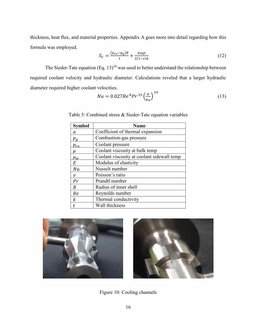
Figure 10: Cooling channels

17

In order to enhance the cooling capabilities, the DPE combustor contains six channels

(Shown in Fig. 10) two millimeters in height and width. Such dimensions minimize the pressure

drop and reduce the required flow rate. The complex geometry of the channels was added to the

combustor using a manufacturing technique known as Electrical Discharge Machining (EDM).

The process consists of removing material form the work-piece using electrical discharges.

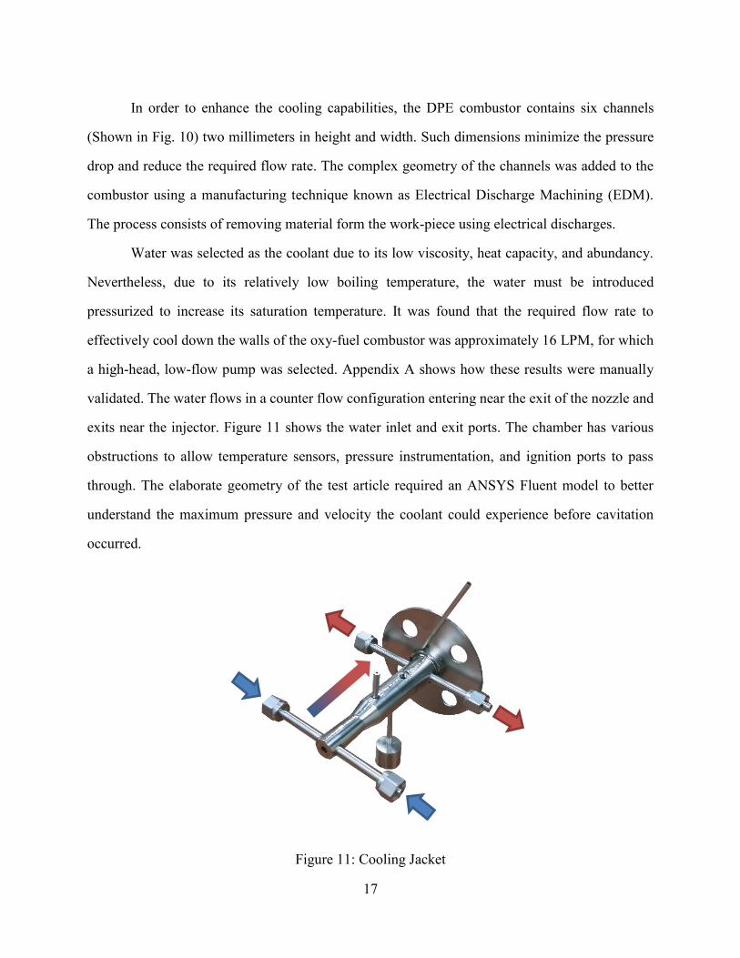
Water was selected as the coolant due to its low viscosity, heat capacity, and abundancy.

Nevertheless, due to its relatively low boiling temperature, the water must be introduced

pressurized to increase its saturation temperature. It was found that the required flow rate to

effectively cool down the walls of the oxy-fuel combustor was approximately 16 LPM, for which

a high-head, low-flow pump was selected. Appendix A shows how these results were manually

validated. The water flows in a counter flow configuration entering near the exit of the nozzle and

exits near the injector. Figure 11 shows the water inlet and exit ports. The chamber has various

obstructions to allow temperature sensors, pressure instrumentation, and ignition ports to pass

through. The elaborate geometry of the test article required an ANSYS Fluent model to better

understand the maximum pressure and velocity the coolant could experience before cavitation

occurred.

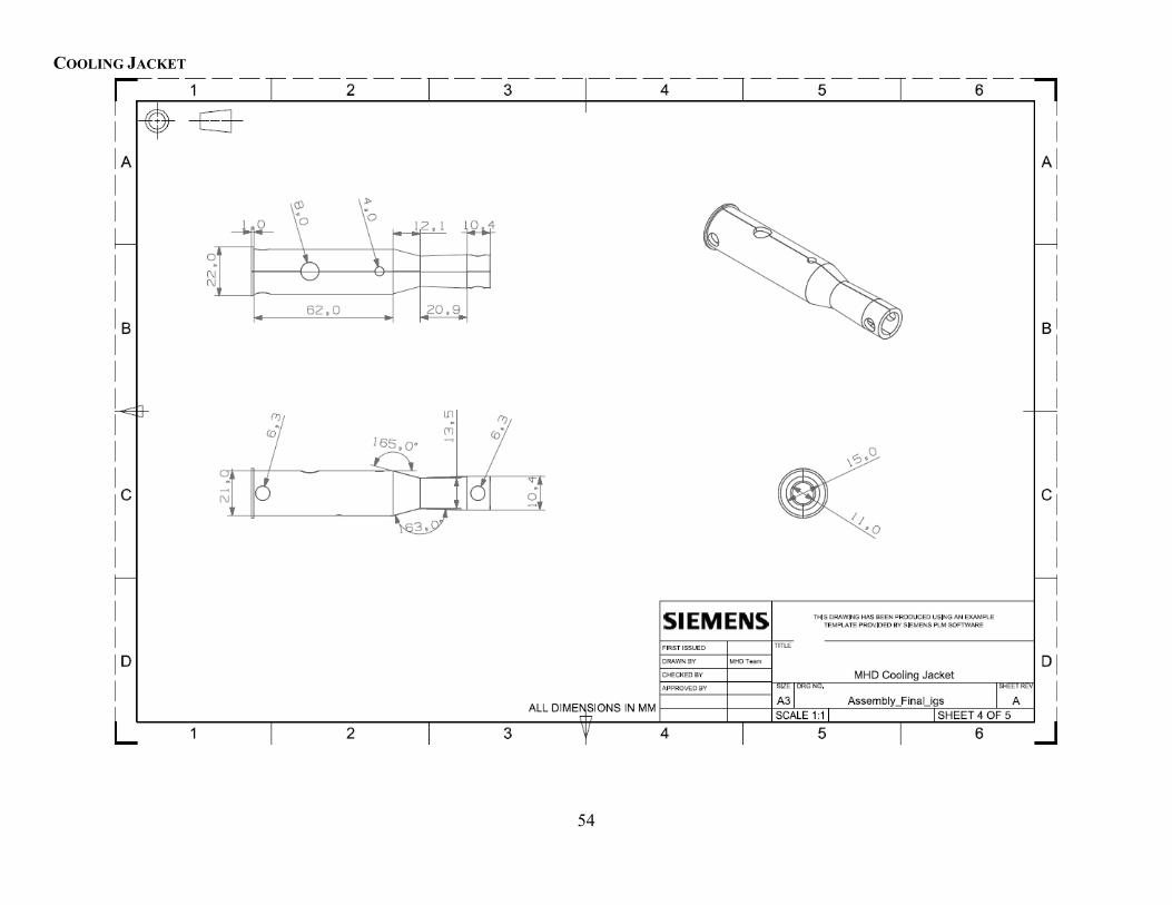
Figure 11: Cooling Jacket

18

In order to simulate the heat transfer occurring in the system, the energy equation is

utilized, Eq. (14)26.

𝜕(𝜌𝐸)

𝜕𝑡+ 𝛻 ∙ [𝑉 (𝜌𝐸 + 𝑝)] = 𝛻 ∙ [𝑘𝑒𝑓𝑓𝛻𝑇 − ∑ ℎ𝑗𝑗 𝐽𝑗 + (𝜏��𝑓𝑓 ∙ 𝑉 )] + 𝑆ℎ (14)

Heat transfer due to conduction, species transport, and viscous dissipation were all

considered for the current project26. The heat conduction through the walls and the heat transfer to

the water is also modeled. Heat convection occurring between the fluid and walls assumed the

cooling fluid (water) was incompressible and neglected kinetic energy and viscous dissipation26.

These assumptions further simplified the energy equation and yielded Eq. (15)26. 𝜕𝑇

𝜕𝑡+ 𝑢

𝜕𝑇

𝜕𝑥+ 𝑣

𝜕𝑇

𝜕𝑦=

𝜆

𝜌𝐶𝑝

𝜕2𝑇

𝜕𝑥2 +𝜆

𝜌𝐶𝑝

𝜕2𝑇

𝜕𝑦2 (15)

Table 6: Cooling system model variables

Symbol Name

𝜌 Density

𝐽𝑗 Diffusion flux of species j

𝑘𝑒𝑓𝑓 Effective conductivity

ℎ𝑗 Enthalpy for species j

𝑃 Pressure

𝐶𝑝 Specific heat

𝑇 Temperature

𝜆 Thermal conductivity

𝑡 Thickness

𝑉 Velocity

𝑆ℎ Volumetric heat source

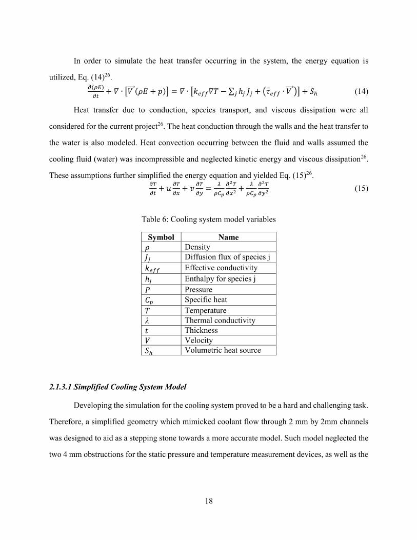
2.1.3.1 Simplified Cooling System Model

Developing the simulation for the cooling system proved to be a hard and challenging task.

Therefore, a simplified geometry which mimicked coolant flow through 2 mm by 2mm channels

was designed to aid as a stepping stone towards a more accurate model. Such model neglected the

two 4 mm obstructions for the static pressure and temperature measurement devices, as well as the

19

8 mm obstruction designated for the spark-igniter port. The geometry also lacked the internal

manifold where the water distributes.

Figure 12: Simplified cooling system model

2.2 MESH

The following section describes the mesh properties for the final models only.

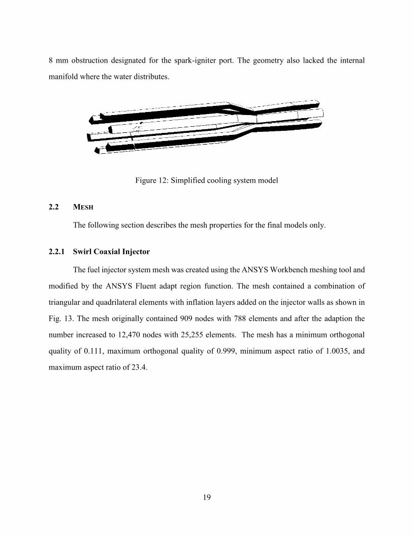
2.2.1 Swirl Coaxial Injector

The fuel injector system mesh was created using the ANSYS Workbench meshing tool and

modified by the ANSYS Fluent adapt region function. The mesh contained a combination of

triangular and quadrilateral elements with inflation layers added on the injector walls as shown in

Fig. 13. The mesh originally contained 909 nodes with 788 elements and after the adaption the

number increased to 12,470 nodes with 25,255 elements. The mesh has a minimum orthogonal

quality of 0.111, maximum orthogonal quality of 0.999, minimum aspect ratio of 1.0035, and

maximum aspect ratio of 23.4.

20

Figure 13: Swirl coaxial injector mesh

2.2.2 Converging-Diverging Nozzle

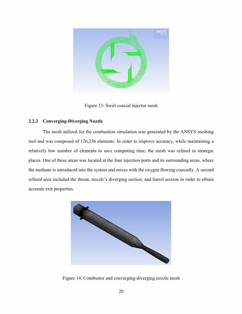
The mesh utilized for the combustion simulation was generated by the ANSYS meshing

tool and was composed of 126,236 elements. In order to improve accuracy, while maintaining a

relatively low number of elements to save computing time, the mesh was refined in strategic

places. One of these areas was located at the four injection ports and its surrounding areas, where

the methane is introduced into the system and mixes with the oxygen flowing coaxially. A second

refined area included the throat, nozzle’s diverging section, and barrel section in order to obtain

accurate exit properties.

Figure 14: Combustor and converging-diverging nozzle mesh

21

2.2.3 Cooling System

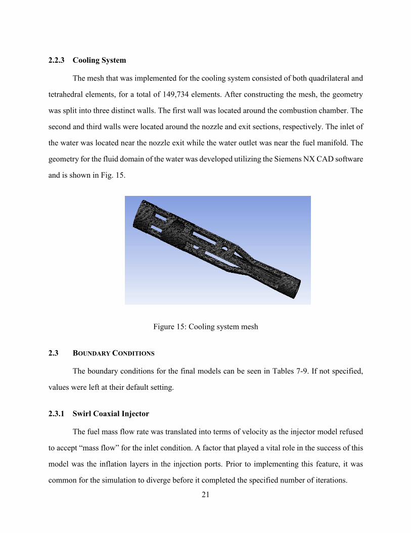
The mesh that was implemented for the cooling system consisted of both quadrilateral and

tetrahedral elements, for a total of 149,734 elements. After constructing the mesh, the geometry

was split into three distinct walls. The first wall was located around the combustion chamber. The

second and third walls were located around the nozzle and exit sections, respectively. The inlet of

the water was located near the nozzle exit while the water outlet was near the fuel manifold. The

geometry for the fluid domain of the water was developed utilizing the Siemens NX CAD software

and is shown in Fig. 15.

Figure 15: Cooling system mesh

2.3 BOUNDARY CONDITIONS

The boundary conditions for the final models can be seen in Tables 7-9. If not specified,

values were left at their default setting.

2.3.1 Swirl Coaxial Injector

The fuel mass flow rate was translated into terms of velocity as the injector model refused

to accept “mass flow” for the inlet condition. A factor that played a vital role in the success of this

model was the inflation layers in the injection ports. Prior to implementing this feature, it was

common for the simulation to diverge before it completed the specified number of iterations.

22

Table 7: Boundary conditions for the swirl coaxial injector

Section Input

General Gravitational acceleration - 9.81 m/s²

Models Multiphase – Volume of fluid

Viscous – Standard k-epsilon

Materials Methane:

Density – 0.6654 kg/m3

Cp – Piecewise-polynomial

Phases Primary – Air

Secondary – Methane

Boundary conditions Mixture inlet:

Velocity - 200 m/s

Hydraulic diameter – 3.05 mm

Methane inlet:

Volume fraction – 1

Mixture outlet:

Pressure - 657.14 kPa

Hydraulic diameter – 1.59 mm

Solution initialization Standard – Inlet

2.3.2 Converging-Diverging Nozzle

The converging-diverging nozzle model took a considerable amount of time to complete.

Often times the simulation would diverge immediately. In other occasions it would complete a

vast amount of iterations, but eventually diverge before reaching steady state. Modifying the

“initial values” under solution initialization was found to solve the issue. The temperature and

velocity were specified to an approximate middle point between the initial and (expected) final

values. Additionally, some under-relaxation factors were applied per suggestion of the official

ANSYS Fluent Tutorial Guide. Appendix A describes how the fuel and oxidizer mass flow rates

were determined.

23

Table 8: Boundary conditions for the converging-diverging nozzle

Section Input

Models Energy – On

Viscous – Standard k-epsilon

Radiation – P1

Species – Non-premixed combustion

Inlet diffusion – On

Compressibility effects – On

Fuel stream reach flammability limit - 0.23

Mass fraction of CH4 – 1

Mass fraction of O2 - 1

Materials PDF mixture

Absorption coefficient – wsggm-domain-based

Boundary conditions Fuel inlet:

Mass flow rate - 0.25025 g/s per orifice

Initial gauge pressure – 657.14 kPa

Hydraulic diameter – 1.59 mm

Mean mixture fraction – 1

Oxidizer inlet:

Mass flow rate – 3.495 g/s

Initial gauge pressure - 657.14 kPa

Hydraulic diameter – 10 mm

Outlet:

Hydraulic diameter – 5 mm

Backflow total temperature – 1500 K

Wall:

Temperature - 525 K

Solution Controls Pressure - 0.9

Body forces - 0.9

Momentum - 0.4

Turbulent kinetic energy - 0.7

P1: 0.5

Solution initialization Standard – Inlet

Gauge pressure - 657.14 kPa

X-velocity - 1000 m/s

Temperature: 1650 K

24

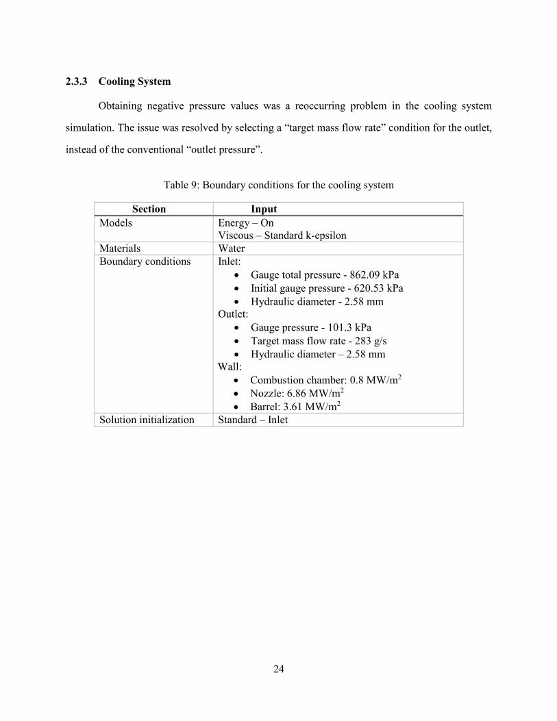
2.3.3 Cooling System

Obtaining negative pressure values was a reoccurring problem in the cooling system

simulation. The issue was resolved by selecting a “target mass flow rate” condition for the outlet,

instead of the conventional “outlet pressure”.

Table 9: Boundary conditions for the cooling system

Section Input

Models Energy – On

Viscous – Standard k-epsilon

Materials Water

Boundary conditions Inlet:

Gauge total pressure - 862.09 kPa

Initial gauge pressure - 620.53 kPa

Hydraulic diameter - 2.58 mm

Outlet:

Gauge pressure - 101.3 kPa

Target mass flow rate - 283 g/s

Hydraulic diameter – 2.58 mm

Wall:

Combustion chamber: 0.8 MW/m2

Nozzle: 6.86 MW/m2

Barrel: 3.61 MW/m2

Solution initialization Standard – Inlet

25

Chapter 3: Results and Discussion

The results for the final models and a few concepts are discussed in this chapter in order to

demonstrate how the design process evolved and evaluate improvements.

3.1 SWIRL COAXIAL INJECTOR

3.1.1 Velocity and Pressure

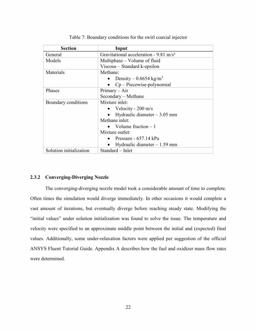
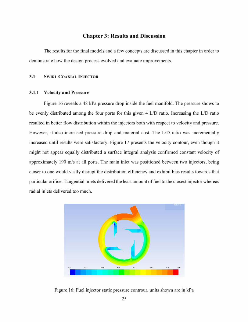
Figure 16 reveals a 48 kPa pressure drop inside the fuel manifold. The pressure shows to

be evenly distributed among the four ports for this given 4 L/D ratio. Increasing the L/D ratio

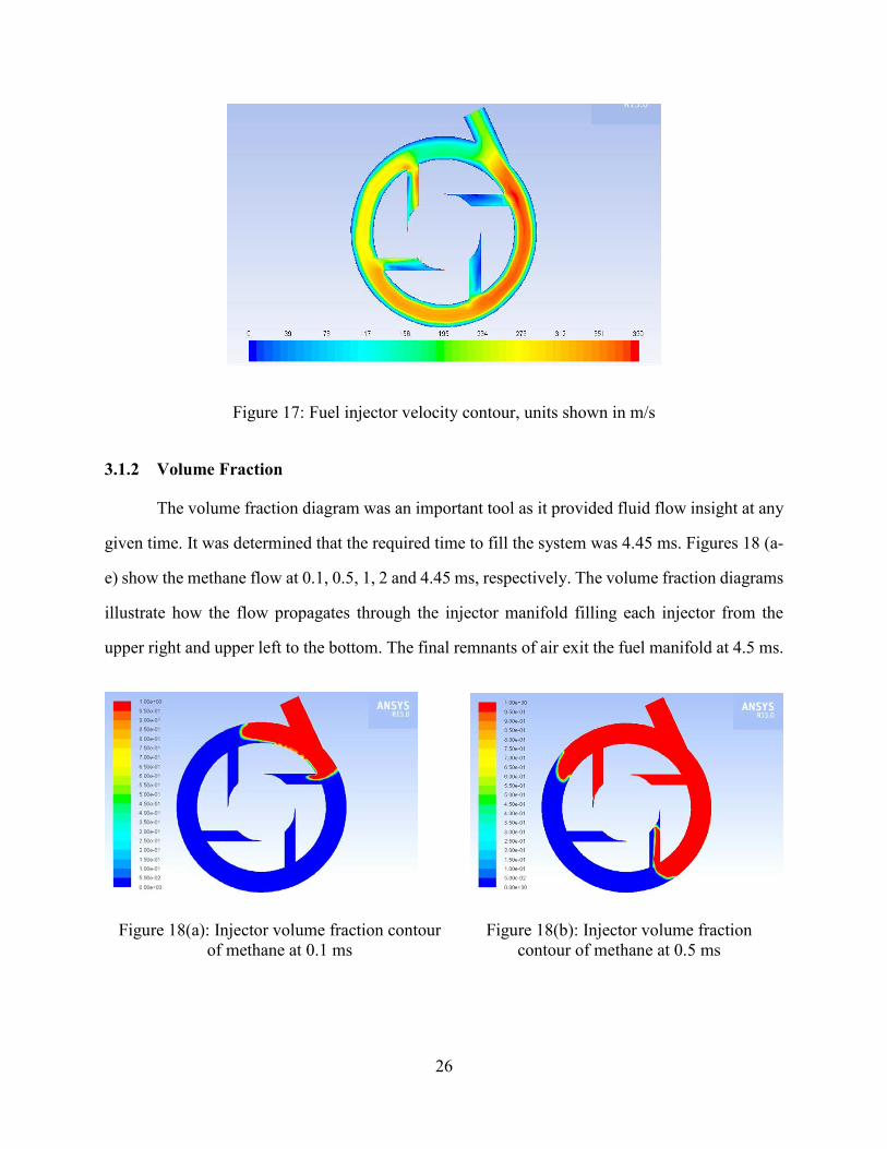
resulted in better flow distribution within the injectors both with respect to velocity and pressure.

However, it also increased pressure drop and material cost. The L/D ratio was incrementally

increased until results were satisfactory. Figure 17 presents the velocity contour, even though it

might not appear equally distributed a surface integral analysis confirmed constant velocity of

approximately 190 m/s at all ports. The main inlet was positioned between two injectors, being

closer to one would vastly disrupt the distribution efficiency and exhibit bias results towards that

particular orifice. Tangential inlets delivered the least amount of fuel to the closest injector whereas

radial inlets delivered too much.

Figure 16: Fuel injector static pressure controur, units shown are in kPa

26

Figure 17: Fuel injector velocity contour, units shown in m/s

3.1.2 Volume Fraction

The volume fraction diagram was an important tool as it provided fluid flow insight at any

given time. It was determined that the required time to fill the system was 4.45 ms. Figures 18 (a-

e) show the methane flow at 0.1, 0.5, 1, 2 and 4.45 ms, respectively. The volume fraction diagrams

illustrate how the flow propagates through the injector manifold filling each injector from the

upper right and upper left to the bottom. The final remnants of air exit the fuel manifold at 4.5 ms.

Figure 18(a): Injector volume fraction contour

of methane at 0.1 ms

Figure 18(b): Injector volume fraction

contour of methane at 0.5 ms

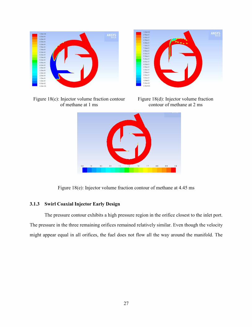
27

Figure 18(e): Injector volume fraction contour of methane at 4.45 ms

3.1.3 Swirl Coaxial Injector Early Design

The pressure contour exhibits a high pressure region in the orifice closest to the inlet port.

The pressure in the three remaining orifices remained relatively similar. Even though the velocity

might appear equal in all orifices, the fuel does not flow all the way around the manifold. The

Figure 18(c): Injector volume fraction contour

of methane at 1 ms

Figure 18(d): Injector volume fraction

contour of methane at 2 ms

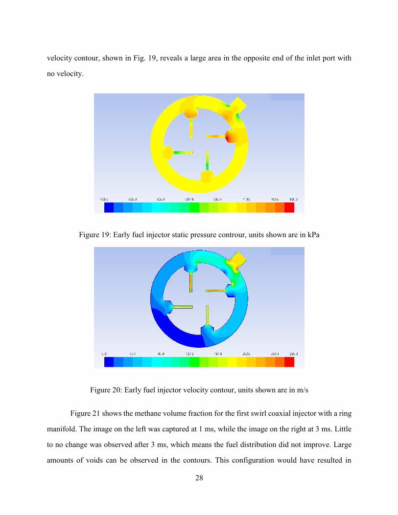
28

velocity contour, shown in Fig. 19, reveals a large area in the opposite end of the inlet port with

no velocity.

Figure 19: Early fuel injector static pressure controur, units shown are in kPa

Figure 20: Early fuel injector velocity contour, units shown are in m/s

Figure 21 shows the methane volume fraction for the first swirl coaxial injector with a ring

manifold. The image on the left was captured at 1 ms, while the image on the right at 3 ms. Little

to no change was observed after 3 ms, which means the fuel distribution did not improve. Large

amounts of voids can be observed in the contours. This configuration would have resulted in

29

combustion instabilities and/or ignition problems. As stated before, the poor distribution efficiency

was attributed to the disturbance in the fluid’s momentum when it enters the manifold and collides

with the wall.

Figure 21: Early injector volume fraction contours of methane at 1 and 3 ms

3.2 CONVERGING-DIVERGING NOZZLE

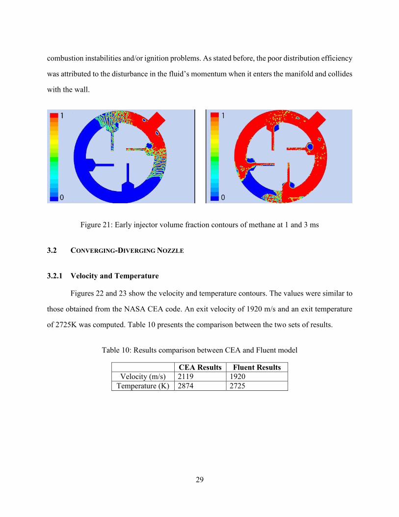
3.2.1 Velocity and Temperature

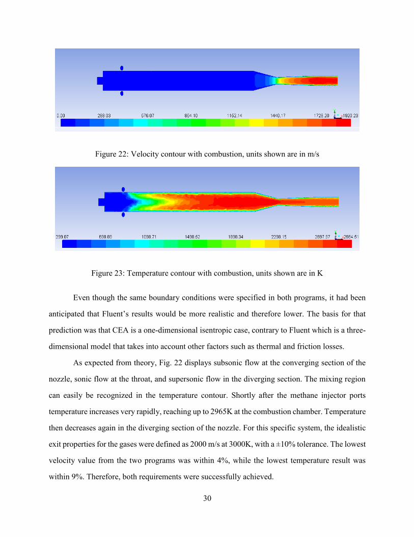
Figures 22 and 23 show the velocity and temperature contours. The values were similar to

those obtained from the NASA CEA code. An exit velocity of 1920 m/s and an exit temperature

of 2725K was computed. Table 10 presents the comparison between the two sets of results.

Table 10: Results comparison between CEA and Fluent model

CEA Results Fluent Results

Velocity (m/s) 2119 1920

Temperature (K) 2874 2725

30

Figure 22: Velocity contour with combustion, units shown are in m/s

Figure 23: Temperature contour with combustion, units shown are in K

Even though the same boundary conditions were specified in both programs, it had been

anticipated that Fluent’s results would be more realistic and therefore lower. The basis for that

prediction was that CEA is a one-dimensional isentropic case, contrary to Fluent which is a three-

dimensional model that takes into account other factors such as thermal and friction losses.

As expected from theory, Fig. 22 displays subsonic flow at the converging section of the

nozzle, sonic flow at the throat, and supersonic flow in the diverging section. The mixing region

can easily be recognized in the temperature contour. Shortly after the methane injector ports

temperature increases very rapidly, reaching up to 2965K at the combustion chamber. Temperature

then decreases again in the diverging section of the nozzle. For this specific system, the idealistic

exit properties for the gases were defined as 2000 m/s at 3000K, with a ±10% tolerance. The lowest

velocity value from the two programs was within 4%, while the lowest temperature result was

within 9%. Therefore, both requirements were successfully achieved.

31

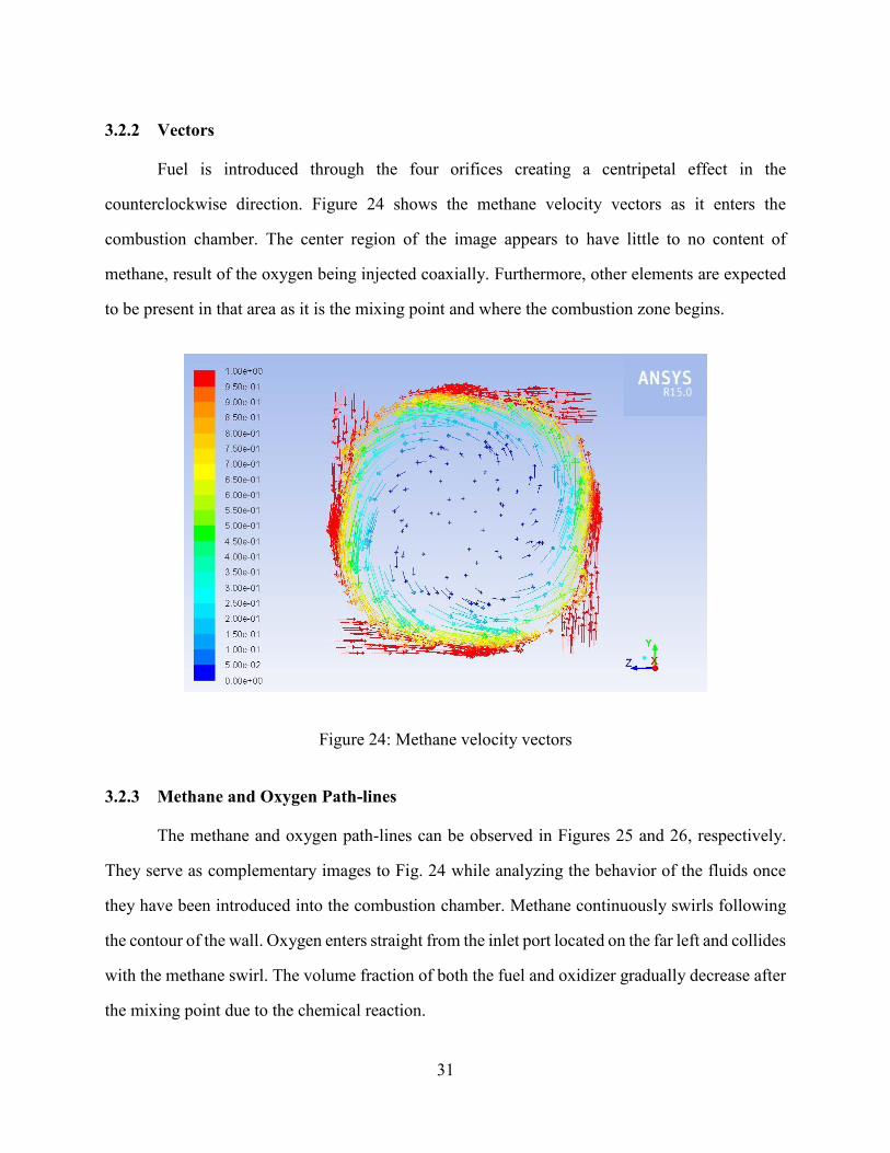
3.2.2 Vectors

Fuel is introduced through the four orifices creating a centripetal effect in the

counterclockwise direction. Figure 24 shows the methane velocity vectors as it enters the

combustion chamber. The center region of the image appears to have little to no content of

methane, result of the oxygen being injected coaxially. Furthermore, other elements are expected

to be present in that area as it is the mixing point and where the combustion zone begins.

Figure 24: Methane velocity vectors

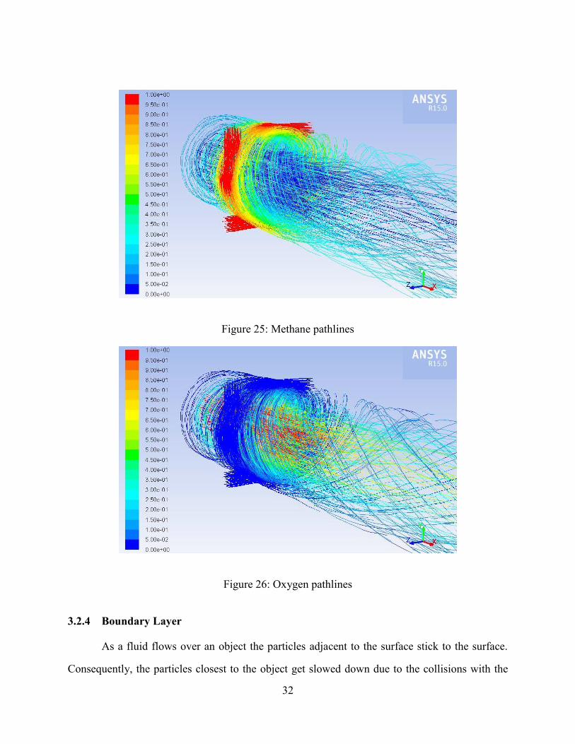
3.2.3 Methane and Oxygen Path-lines

The methane and oxygen path-lines can be observed in Figures 25 and 26, respectively.

They serve as complementary images to Fig. 24 while analyzing the behavior of the fluids once

they have been introduced into the combustion chamber. Methane continuously swirls following

the contour of the wall. Oxygen enters straight from the inlet port located on the far left and collides

with the methane swirl. The volume fraction of both the fuel and oxidizer gradually decrease after

the mixing point due to the chemical reaction.

32

Figure 25: Methane pathlines

Figure 26: Oxygen pathlines

3.2.4 Boundary Layer

As a fluid flows over an object the particles adjacent to the surface stick to the surface.

Consequently, the particles closest to the object get slowed down due to the collisions with the

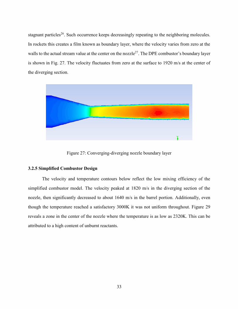
33

stagnant particles26. Such occurrence keeps decreasingly repeating to the neighboring molecules.

In rockets this creates a film known as boundary layer, where the velocity varies from zero at the

walls to the actual stream value at the center on the nozzle27. The DPE combustor’s boundary layer

is shown in Fig. 27. The velocity fluctuates from zero at the surface to 1920 m/s at the center of

the diverging section.

Figure 27: Converging-diverging nozzle boundary layer

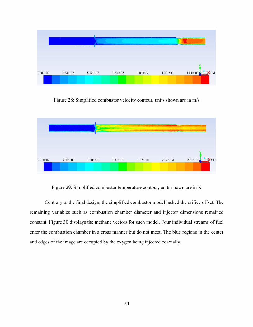
3.2.5 Simplified Combustor Design

The velocity and temperature contours below reflect the low mixing efficiency of the

simplified combustor model. The velocity peaked at 1820 m/s in the diverging section of the

nozzle, then significantly decreased to about 1640 m/s in the barrel portion. Additionally, even

though the temperature reached a satisfactory 3000K it was not uniform throughout. Figure 29

reveals a zone in the center of the nozzle where the temperature is as low as 2320K. This can be

attributed to a high content of unburnt reactants.

34

Figure 28: Simplified combustor velocity contour, units shown are in m/s

Figure 29: Simplified combustor temperature contour, units shown are in K

Contrary to the final design, the simplified combustor model lacked the orifice offset. The

remaining variables such as combustion chamber diameter and injector dimensions remained

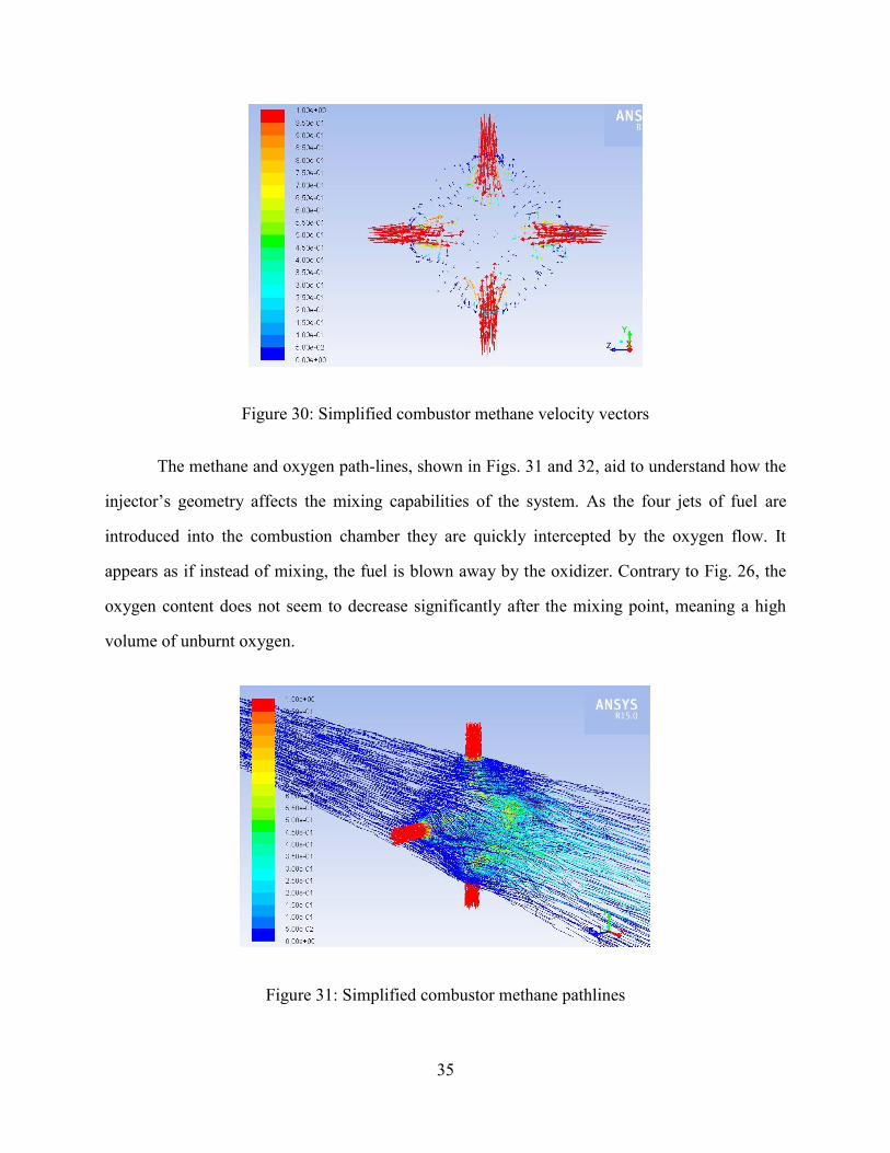
constant. Figure 30 displays the methane vectors for such model. Four individual streams of fuel

enter the combustion chamber in a cross manner but do not meet. The blue regions in the center

and edges of the image are occupied by the oxygen being injected coaxially.

35

Figure 30: Simplified combustor methane velocity vectors

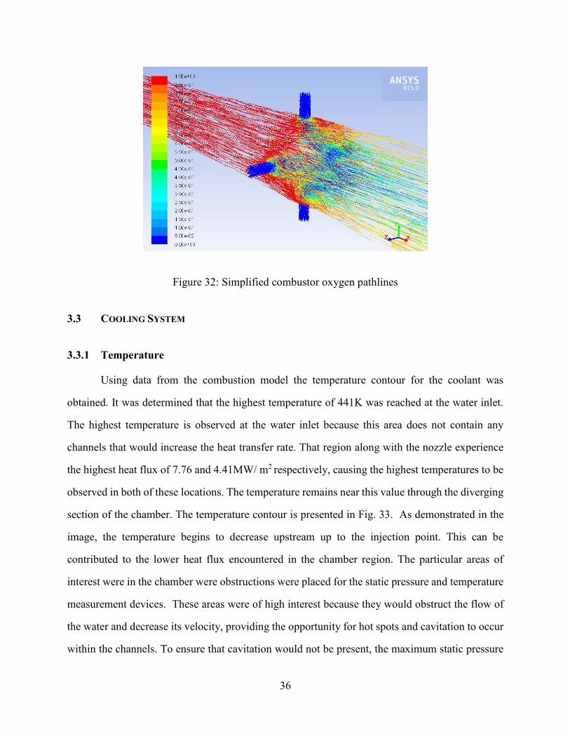
The methane and oxygen path-lines, shown in Figs. 31 and 32, aid to understand how the

injector’s geometry affects the mixing capabilities of the system. As the four jets of fuel are

introduced into the combustion chamber they are quickly intercepted by the oxygen flow. It

appears as if instead of mixing, the fuel is blown away by the oxidizer. Contrary to Fig. 26, the

oxygen content does not seem to decrease significantly after the mixing point, meaning a high

volume of unburnt oxygen.

Figure 31: Simplified combustor methane pathlines

36

Figure 32: Simplified combustor oxygen pathlines

3.3 COOLING SYSTEM

3.3.1 Temperature

Using data from the combustion model the temperature contour for the coolant was

obtained. It was determined that the highest temperature of 441K was reached at the water inlet.

The highest temperature is observed at the water inlet because this area does not contain any

channels that would increase the heat transfer rate. That region along with the nozzle experience

the highest heat flux of 7.76 and 4.41MW/ m2 respectively, causing the highest temperatures to be

observed in both of these locations. The temperature remains near this value through the diverging

section of the chamber. The temperature contour is presented in Fig. 33. As demonstrated in the

image, the temperature begins to decrease upstream up to the injection point. This can be

contributed to the lower heat flux encountered in the chamber region. The particular areas of

interest were in the chamber were obstructions were placed for the static pressure and temperature

measurement devices. These areas were of high interest because they would obstruct the flow of

the water and decrease its velocity, providing the opportunity for hot spots and cavitation to occur

within the channels. To ensure that cavitation would not be present, the maximum static pressure

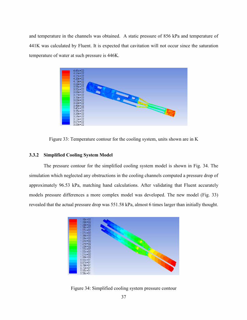
37

and temperature in the channels was obtained. A static pressure of 856 kPa and temperature of

441K was calculated by Fluent. It is expected that cavitation will not occur since the saturation

temperature of water at such pressure is 446K.

Figure 33: Temperature contour for the cooling system, units shown are in K

3.3.2 Simplified Cooling System Model

The pressure contour for the simplified cooling system model is shown in Fig. 34. The

simulation which neglected any obstructions in the cooling channels computed a pressure drop of

approximately 96.53 kPa, matching hand calculations. After validating that Fluent accurately

models pressure differences a more complex model was developed. The new model (Fig. 33)

revealed that the actual pressure drop was 551.58 kPa, almost 6 times larger than initially thought.

Figure 34: Simplified cooling system pressure contour

38

Chapter 4: Summary and Conclusions

Recent interest in efficient and low-pollution power generation has led to investigation of

various energy producing devices. A technology that lost attractiveness among investors in the 20th

century and now being revisited is magnetohydrodynamics (MHD). MHD power generators

extract electrical energy directly from gases flowing through a magnetic field. Some advantages

of these systems include:

Higher efficiency due to the lack of mechanical components

Potential to reach higher efficiencies than those of coal burning

Higher thermal efficiencies associated with oxy-fuel combustion

The system eliminates toxic combustion residuals making H2O and CO2 the only

products, from which CO2 can be sequestered

MHD generators can be retrofitted into existing power plants, using the exhaust

gases as energy source to generate steam

Some of the disadvantages are:

Producing pure oxygen requires a lot of energy

MHD generators are still in early stages and need more development

For this paper the modeling of various components of an MHD device are presented. This

includes the fuel injector, combustor, nozzle, and cooling system. The main findings from this

study are:

In the fuel injector the counter-swirl inlets achieve a uniform pressure and velocity

distribution when the L/D ratio is 4. Changes in the inlet location and orientation

impacted pressure and velocity distribution. An angle of 115° in respect to the x-

axis was found to increase distribution efficiency.

Both the velocity and temperature criteria of 2000 m/s and 3000K ±10% were

successfully achieved with the combustor. Data from NASA CEA and Fluent

39

matched within 4% and 9%, respectively. Differences may be attributed to CEA

assumption of one-dimensional isentropic flow.

A static pressure of 856 kPa and temperature of 441 K was calculated by Fluent. It

is expected that cavitation will not occur since the saturation temperature of water

at such pressure is 446K. It was also determined that the water flowed at an

approximate volumetric flow rate of 17 LPM at an initial pressure of approximately

758.42 kPa. This will ensure that the cooling system will work effectively and the

overall system will not fail.

While developing the various simulations it was always useful to start with a basic model

and gradually add details making it more accurate. The simplicity of these models made it possible

to validate Fluent’s results by hand, proportioning confidence on the results of their more complex

counterparts. They also permitted to freely explore different combinations of boundary conditions

to find the ones that worked best.

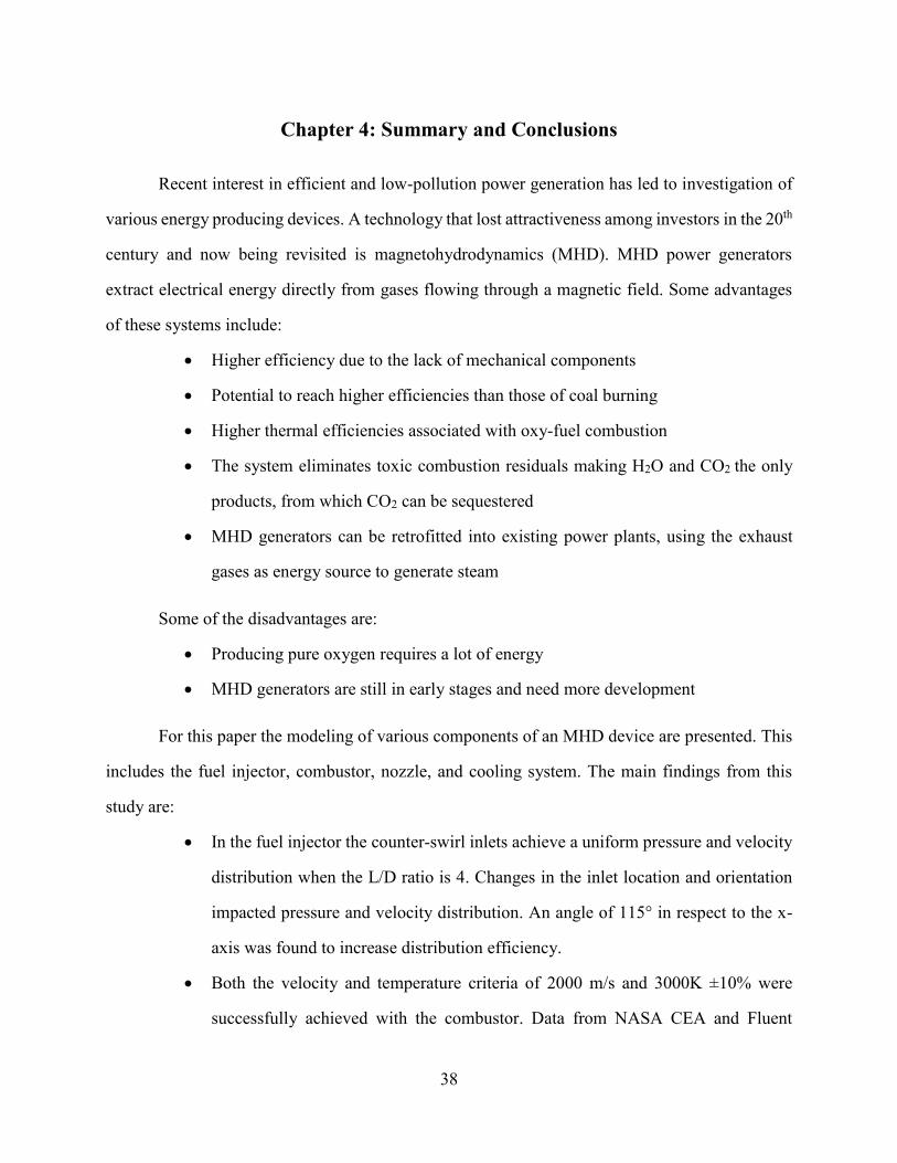
Figure 35: DPE combustor

40

References

12013 EPA Reports retrieved from

https://www.epa.gov/climatechange/ghgemissions/usinventoryreport.html 2Human Health and Environmental Effects of Emissions from Power Generation retrieved

from https://www.epa.gov/captrade/documents/power.pdf 3Hunt, R., “The History of the Industrial Gas Turbine (Part 1 the first fifty years)”. The

Independent Technical Forum for Power Generation, Vol. 582, 2011. 4Battery and Energy Technologies. (n.d.). Retrieved from

https://www.mpoweruk.com/mhd_generator.html 5Richards, G. A. (2013, July). Future Combustion Technologies: Chemical Looping

Combustion Direct Power Extraction Pressure gain combustion. Retrieved from

https://www.netl.doe.gov/File Library/events/2013/co2 capture/G-Richards-NETL-Future-

Combustion.pdf 6Liu, BL, et al. "Three-Dimensional Analysis of the IEE MARK II MHD Generator". 9th

International Conference on Magnetohydro-dynamic Electric Power Generation. Web. 7Malghan, V. , “History of MHD Power Plant Development” Energy Conversion and

Management, Vol. 37, No. 5, May 1996, pp. 569-590. 8Anghaie, S., and Saraph, G., “Conceptual Design Analysis of An MHD Power Conversion

System for Droplet-Vapor Core Reactors” Innovative Nuclear Space Power Institute DE-

FG0593ER75871, 1995. 9Petrick M, Shumyatsky BYa, editors. Open-cycle magnetohydrodynamic electrical power

generation. Technical and economic aspects of open-cycle MHD power plants, Nauka, Moscow

and Argonne NL: Joint US–USSR Publication; 1978. 10Way, S., and Hundstad, R. , “Direct Generation of Power from a Combustion Gas Stream”,

Symposium (International) on Combustion, Vol.8, No.1, 1991, pp.241-251. 11Velikhov, E. P., Pismenny, V. D., Pisakin, A. V., Zhukov, B. B., and Sukharev, E. M. , “Pulsed

MHD Power System SAKHALIN-The World Largest Solid Propellant Fueled MHD Generator of

500MWe Electric Power Output.” Proceedings of 13th International Conference on MHD Power

Generation and High Temperature Technologies, Vol. 2, pp. 387-398. 1999 12Klepeis, James, and Vladimir Hruby. "MHD power generation experiments with a large disk

channel-Verification of disk scaling laws." Engineering Aspects of Magnetohydrodynamics. Vol.

1. 1976 13Felderman, E. J., et. al., "HPDE Performance in the Faraday Mode", 20th EAMHD.

Symposium, Irvine CA, June 1982, paper 4, 5. 14Aithal, S. , “Analysis of Optimum Power Extraction in a MHD Generator with Spatially

Varying Electrical Conductivity, International Journal of Thermal Sciences, 2008, Vol.47, No.8,

pp.1107-1112. 15Ishikwa, M., and Yuhara, M. , “Three-Dimensional Computation of Magnetohydrodynamics

in Weakly Ionized Plasma with Strong MHD Interaction”, Journal of Materials Processing

Technology, 2007,Vol. 181, No.1-3, pp. 254-259. 16Bhadoria, B., and Chandra, A. , “Transient Analysis of Proposed Indian MHD Channel”

Energy Conversion and Management, 2001, Vol. 42, No.8, pp. 963-966. 17Wolfendale, M. , “A Coupled Systems Code-CFD MHD Solver for Fusion Blanket Design”,

Fusion Engineering and Design, October 2015, Vol. 98-99, pp. 1902-1906

41

18Zubanov, V., and Egorychev, V. , “Design of Rocket for Spacecraft Using CFD- Modeling”

Scientific and Technological Experiments on Automatic Space Vehicles and Small Satellites,

Vol.104, pp. 29-35. 19Hernandez, M., Cabrera, L., Vidaña, O., Chaidez, M., Love, N., and Choudhuri, A., "Design

of an Oxy-Methane Combustor for Direct Power Extraction," AIAA-2016-0243, 2016

20Wendt, J. , Governing Equations of Fluid Mechanics in Computational Fluid Dynamics an

Introduction, 3rd ed., Springer,Berlin, 2009. 21Flow of fluids through valves, fittings, and pipe. (1969). New York: Engineering Division

Crane. 22NASA Chemical Equilibrium with Applications (CEA). (n.d.). Retrieved from

http://www.grc.nasa.gov/WWW/CEAWeb 23Non-Premixed Combustion. (2013). In ANSYS Fluent Theory Guide (pp. 215-218). 24Huang, D.H., and Huzel, D.K, Modern Engineering for Design of Liquid Propellant Rocket

Engines, American Institute of Aeronautics and Astronautics, Washington D.C., 1992. 25Betti, B., Nasuti, F., & Martelli, E. “Numerical simulation of hot-gas side heat transfer

enhancement in thrust chambers by wall ribs” AIAA Paper, 5622, 2011. 26Tu, J., & Yeoh, G., Computational Fluid Dynamics a Practical Approach 2nd ed.,

Butterworth-Heinemann, Waltham MA., 2008. 27Boundary Layer. (n.d.). Retrieved from https://www.grc.nasa.gov/www/k-

12/airplane/boundlay.html 28Cengel, Y. A., & Cimbala, J. M. (2006). Fluid mechanics: Fundamentals and applications.

Boston: McGraw-HillHigher Education. 29Vidaña, O., Chaidez, M., Lovich, B., Aboud, J., Hernandez, M., Cabrera, L., Love, N., and

Choudhuri, A., "Component and System Modeling of a Direct Power Extraction System," AIAA-

2016-0990, 2016

42

Appendix A: Sample Calculations

FUEL & OXIDIZER MASS FLOW RATES

The first step was to balance the chemical reaction between Methane and Oxygen:

𝐶𝐻4 + 𝑂2 → 𝐶𝑂2+𝐻2𝑂

𝐶𝐻4 + 2𝑂2 → 𝐶𝑂2+2𝐻2𝑂

Oxygen and Methane have a molecular weight of 15.9994 and 16.04 g/mol, respectively.

This means that 16.04 grams of methane react with 63.9976 grams of oxygen. Stoichiometric ratio

is: 𝑂

𝐹= 3.99

However, it was decided for the DPE combustor to operate at a slightly rich equivalence

ratio of 1.14. This yielded a mixture ratio of 3.49. Knowing this value allowed to develop a

relationship between total and fuel mass flow rate. ��𝑂

��𝐹= 3.49

��𝑇 = ��𝐹 + ��𝑂 → ��𝑇 = ��𝐹(1 + 3.49) →��𝑇

��𝐹= 4.49

CEA provided the velocity (1177.2 m/s) and density (0.35522 kg/m3) at the throat. Using

that information and assuming a throat diameter of 3.68 mm total mass flow rate was computed:

��𝑇 = 𝜌𝐴𝑉 = 𝟎. 𝟎𝟎𝟒𝟒𝟗𝟔 𝒌𝒈/𝒔

It was then possible to calculate the methane and oxygen individual flow rates:

��𝐹 =��𝑇

4.49= 𝟎. 𝟎𝟎𝟏𝟎𝟎𝟏 𝒌𝒈/𝒔

��𝑂 = 3.49 ∗ ��𝐹 = 𝟎. 𝟎𝟎𝟑𝟒𝟗𝟓 𝒌𝒈/𝒔

43

Table 11: Flow rate calculation variables

Symbol Name Units

𝐴 Area m2

𝜌 Density kg/m3

��𝐹 Methane mass flow rate kg/s

��𝑂 Oxygen mass flow rate kg/s

��𝑇 Total mass flow rate kg/s

𝑉 Velocity m/s

THROAT CONDITIONS

The first step while calculating the throat’s local heat flux was using Bartz Correlation to

find the heat transfer coefficient24:

ℎ𝑔 = [0.026

𝐷𝑡0.2 (

𝜇0.2𝑐𝑝

𝑃𝑟0.6) (

(𝑝𝑐)𝑔

𝑐∗) (

𝐷𝑡

𝑅)

0.1

] ×𝐴𝑡

𝐴

0.9

𝜎

Some variables such as 𝐷𝑡, R, 𝐴𝑡, A were directly dependent on the combustor’s geometry.

The rest of the values were retrieved from CEA after making the following set of assumptions;

equivalence ratio of 1.14, chamber pressure of 758.42 kPa and expansion ratio of 1.85.

In order to calculate 𝜎 the following formula was employed24:

𝜎 =1

[12

𝑇𝑤𝑔

𝑇𝑐(1 +

𝛾 − 12 𝑀2) +

12]0.68[1 +

𝛾 − 12 𝑀2]0.12

𝑇𝑤𝑔 was set to 525 °C due to Inconel 718’s thermal properties, and M to 1 since the point

of interest was the throat. The remaining values were acquired from CEA. This yielded an ℎ𝑔 of

4544 W/m2-K. However, as previously explained Bartz correlation tends to overestimate the

convective heat transfer coefficient, for which it was reduced by 40%.

ℎ𝑔 × 0.6 = 𝟐𝟕𝟐𝟔 𝐖/𝐦²𝐊

Once ℎ𝑔 was corrected, the heat flux could be calculated24:

𝑞 = ℎ𝑔(𝑇𝑎𝑤 − 𝑇𝑤𝑔) = 𝟔. 𝟖𝟔 𝑴𝑾/𝒎²

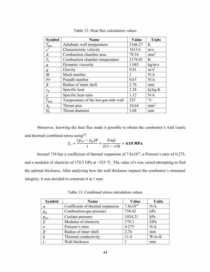
44

Table 12: Heat flux calculation values

Symbol Name Value Units

𝑇𝑎𝑤 Adiabatic wall temperature 3146.27 K

𝑐∗ Characteristic velocity 1813.6 m/s

𝐴 Combustion chamber area 78.54 mm2

𝑇𝑐 Combustion chamber temperature 3178.05 K

𝜇 Dynamic viscosity 1.043 kg/m-s

𝑔 Gravity 9.81 m/s2

𝑀 Mach number 1 N/A

𝑃𝑟 Prandtl number 0.67 N/A

𝑅 Radius of inner shell 2.76 mm

𝑐𝑝 Specific heat 2.28 kj/kg-K

𝛾 Specific heat ratio 1.12 N/A

𝑇𝑤𝑔 Temperature of the hot-gas-side wall 525 °C

𝐴𝑡 Throat area 10.64 mm2

𝐷𝑡 Throat diameter 3.68 mm

Moreover, knowing the heat flux made it possible to obtain the combustor’s wall (static

and thermal) combined stress using24:

𝑆𝑐 =(𝑝𝑐𝑜 − 𝑝𝑔)𝑅

𝑡+

𝐸𝑎𝑞𝑡

2(1 − 𝑣)𝑘= 𝟔𝟏𝟎 𝐌𝐏𝐚

Inconel 718 has a coefficient of thermal expansion of 7.8x10-6, a Poisson’s ratio of 0.275,

and a modulus of elasticity of 170.3 GPa at ~525 °C. The value of t was varied attempting to find

the optimal thickness. After analyzing how the wall thickness impacts the combustor’s structural

integrity, it was decided to constrain it at 1 mm.

Table 13: Combined stress calculation values

Symbol Name Value Units

𝑎 Coefficient of thermal expansion 7.8x10-6 N/A

𝑝𝑔 Combustion-gas pressure 758.42 kPa

𝑝𝑐𝑜 Coolant pressure 1034.21 kPa

𝐸 Modulus of elasticity 170.3 GPa

𝑣 Poisson’s ratio 0.275 N/A

𝑅 Radius of inner shell 2.76 mm

𝑘 Thermal conductivity 11.4 W/m-K

𝑡 Wall thickness 1 mm

45

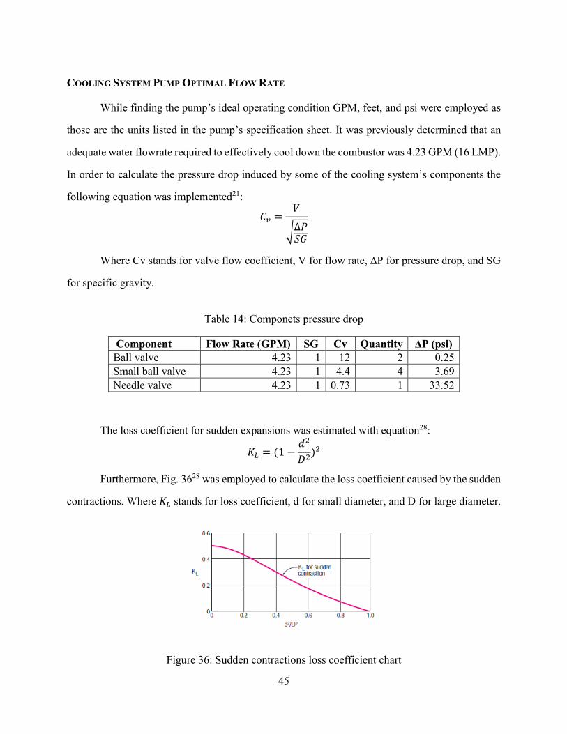
COOLING SYSTEM PUMP OPTIMAL FLOW RATE

While finding the pump’s ideal operating condition GPM, feet, and psi were employed as

those are the units listed in the pump’s specification sheet. It was previously determined that an

adequate water flowrate required to effectively cool down the combustor was 4.23 GPM (16 LMP).

In order to calculate the pressure drop induced by some of the cooling system’s components the

following equation was implemented21:

𝐶𝑣 =𝑉

√∆𝑃𝑆𝐺

Where Cv stands for valve flow coefficient, V for flow rate, ∆P for pressure drop, and SG

for specific gravity.

Table 14: Componets pressure drop

Component Flow Rate (GPM) SG Cv Quantity ΔP (psi)

Ball valve 4.23 1 12 2 0.25

Small ball valve 4.23 1 4.4 4 3.69

Needle valve 4.23 1 0.73 1 33.52

The loss coefficient for sudden expansions was estimated with equation28:

𝐾𝐿 = (1 −𝑑2

𝐷2)2

Furthermore, Fig. 3628 was employed to calculate the loss coefficient caused by the sudden

contractions. Where 𝐾𝐿 stands for loss coefficient, d for small diameter, and D for large diameter.

Figure 36: Sudden contractions loss coefficient chart

46

Next, the head loss was calculated using equation28:

ℎ𝐿 = 𝐾𝐿

𝑉2

2𝑔

Where ℎ𝐿 stands for head loss, V for velocity, and g for gravity.

With that information it was possible to obtain the pressure drop using relationship28:

∆𝑃 = 𝜌𝑔ℎ𝐿

The same process was followed to approximate the pressure drop caused by the multiple

bends.

Table 15: Sudden expanison, sudden contraciton and bends pressure drop

Type d (ft.) D (ft.) 𝑲𝑳 Velocity

(ft/s)

𝒉𝑳 (ft) Quantity ΔP (psi)

Sudden expansion 0.0125 0.029 0.63 33.73 6.66 1 4.79

Sudden contraction 0.0125 0.029 0.42 33.73 0.3 1 3.22

Sudden contraction (2) 0.029 0.083 0.46 14.11 0.43 1 0.62

90° bends N/A N/A 0.3 14.11 0.23 15 6.02

180° bends N/A N/A 0.2 7.05 0.05 2 0.13

Major losses were computed implementing Darcy’s equation28:

∆𝑃 = 𝑓𝐿

𝐷

𝜌𝑉2

2= 33.77 psi

Where f stands for friction factor, L for pipe length, D for hydraulic diameter, and ρ for

density. The flow resulted to be turbulent, for which the friction factor was acquired by means of

the Moody Chart.

Table 16: Pressure drop along the pipes

The test article’s pressure drop was also taken into account, according to Fluent it was

approximately 80 psi. Once the total pressure drop was obtained (148 psi), it was translated into

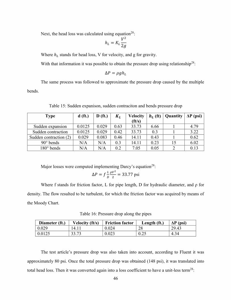
total head loss. Then it was converted again into a loss coefficient to have a unit-less term28:

Diameter (ft.) Velocity (ft/s) Friction factor Length (ft.) ΔP (psi)

0.029 14.11 0.024 28 29.43

0.0125 33.73 0.023 0.25 4.34

47

ℎ𝐿 =∆𝑃

𝜌𝑔=341.31 ft. 𝐾𝐿 =

ℎ𝐿

(𝑉2

2𝑔)

= 110.59

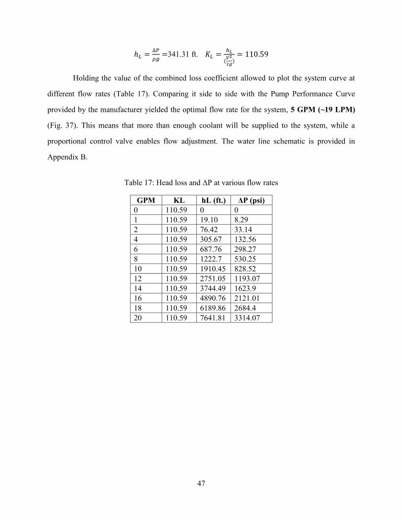
Holding the value of the combined loss coefficient allowed to plot the system curve at

different flow rates (Table 17). Comparing it side to side with the Pump Performance Curve

provided by the manufacturer yielded the optimal flow rate for the system, 5 GPM (~19 LPM)

(Fig. 37). This means that more than enough coolant will be supplied to the system, while a

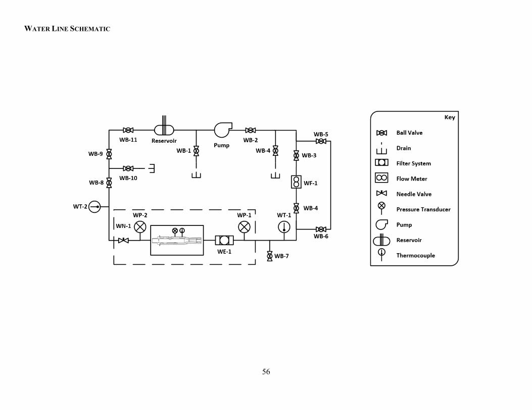
proportional control valve enables flow adjustment. The water line schematic is provided in

Appendix B.

Table 17: Head loss and ΔP at various flow rates

GPM KL hL (ft.) ΔP (psi)

0 110.59 0 0

1 110.59 19.10 8.29

2 110.59 76.42 33.14

4 110.59 305.67 132.56

6 110.59 687.76 298.27

8 110.59 1222.7 530.25

10 110.59 1910.45 828.52

12 110.59 2751.05 1193.07

14 110.59 3744.49 1623.9

16 110.59 4890.76 2121.01

18 110.59 6189.86 2684.4

20 110.59 7641.81 3314.07

48

Figure 37: Pump performance curve vs. System curve

0

100

200

300

400

500

600

700

020406080

100120140160180200220240260280300

0 1 2 3 4 5 6 7 8 9 10 11 12 13 14 15 16 17 18 19 20 21 22

DYN

AM

IC H

EAD

(ft

.)

DYN

AM

IC H

EAD

(p

si)

GPM

Performance Plot

Pump Performance Curve System Curve

49

CEA RESULTS

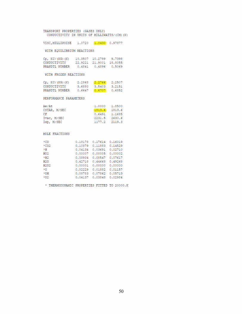
50

51

Appendix B: CADs and Schematics

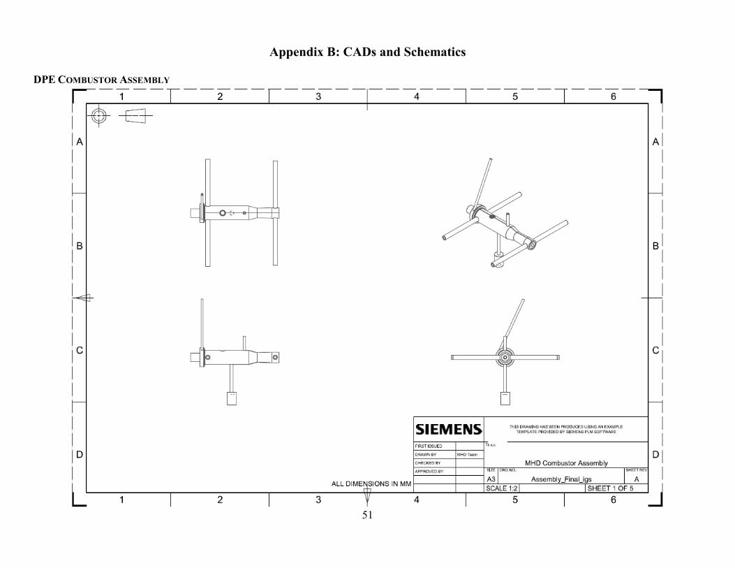
DPE COMBUSTOR ASSEMBLY

52

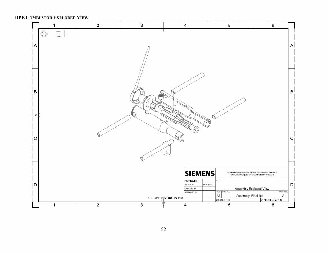
DPE COMBUSTOR EXPLODED VIEW

53

DPE COMBUSTOR

54

COOLING JACKET

55

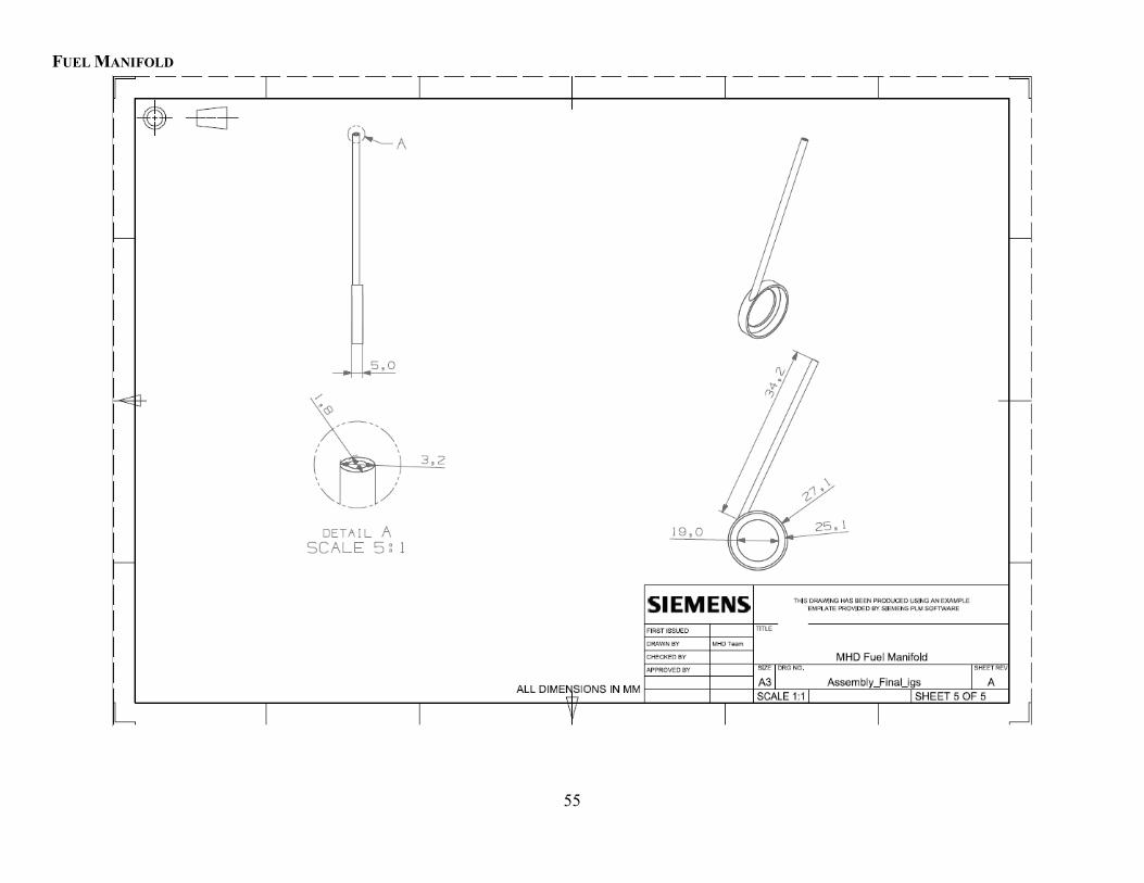
FUEL MANIFOLD

56

WATER LINE SCHEMATIC

57

Vita

Omar D. Vidaña was born in El Paso, Texas, on May 14, 1990. Shortly after that, his family

moved to Zacatecas, Mexico where he lived until he was 10 years old. Following high-school

graduation, he joined the University of Texas at El Paso to pursue a career in Mechanical

Engineering. After earning his Bachelor’s degree in May of 2014, he decided to continue his

education by enrolling a graduate program at the same institution. A few months later, he was

employed as a Research Assistant at the Center for Space Exploration Technology Research Lab

under Dr. Norman Love. There he was teamed with a group of graduate students to develop and

supersonic, liquid-cooled combustor, intended to be used in a direct power extraction system. His

work during the project resulted in three publications, one of them was awarded best paper by the

AIAA Terrestrial Committee at the 2016 SciTech Conference in San Diego, California. On

August, 2016 he was given the title of Master of Science in Mechanical Engineering.

Permanent address: 5465 Gate Ridge Cir.

El Paso, Texas, 79932

This thesis was typed by Omar D. Vidaña