A COMPUTATION OF KNOT FLOER HOMOLOGYOF SPECIAL (1,1)-KNOTS

Jiangnan Yu

Department of MathematicsCentral European University

Advisor: Andras Stipsicz

Proposal prepared by Jiangnan Yu in part fulfillment of the degreerequirements for the Master of Science in Mathematics.

1

CE

UeT

DC

olle

ctio

n

Acknowledgements

I would like to thank Professor Andras Stipsicz for his guidance onwriting this thesis, and also for his teaching and helping during themaster program. From him I have learned a lot knowledge in topol-ogy.

I would also like to thank Central European University and the De-partment of Mathematics for accepting me to study in Budapest.

Finally I want to thank my teachers and friends, from whom I havelearned so much in math.

2

CE

UeT

DC

olle

ctio

n

Abstract

We will introduce Heegaard decompositions and Heegaard diagrams for three-manifoldsand for three-manifolds containing a knot. We define (1,1)-knots and explain the method toobtain the Heegaard diagram for some special (1,1)-knots, and prove that torus knots and 2-bridge knots are (1,1)-knots. We also define the knot Floer chain complex by using the theoryof holomorphic disks and their moduli space, and give more explanation on the chain complexof genus-1 Heegaard diagram. Finally, we compute the knot Floer homology groups of thetrefoil knot and the (-3,4)-torus knot.

1 Introduction

Knot Floer homology is a knot invariant defined by P. Ozsvath andZ. Szabo in [6], using methods of Heegaard diagrams and modulitheory of holomorphic discs, combined with homology theory.

Given a closed, connected, oriented three manifold Y , the Heegaarddecomposition of Y is a decomposition into two handlebodies U0, U1

such that ∂U0 = −∂U1 = Σ and Y = U0 ∪Σ U1. The decomposi-tion is determined by specifying a connnected, closed, oriented two-manifold Σ of genus g and two collections of curves {α1, ..., αg},{β1, ..., βg}.In the second section we will give the definition of a (1,1)-knot, de-scribe how to get Heegaard diagram for (1,1)-knots using methodfrom [3], and give parametrization for (1,1)-knots. Later, we willprove that torus knots are (1,1)-knots, and define another kind ofknots called 2-bridge knots, and prove that they are (1,1)-knots.

Then we will use the Heegaard diagram to define the chain com-plex and the differential map. The differential relies on countingholomorphic disks in the symmetric product Symg(Σ). After these

3

CE

UeT

DC

olle

ctio

n

definition we will compute the homology of the trefoil knot and (-3,4)-torus knot.

2 Heegaard Decomposition

Definition 2.1. Equip Y with a self indexing Morse function f : Y →[0, 3] with one minimum and one maximum, and let Σ = f−1(3

2)

be a genus g surface. Then f induces a Heegaard decompositionY = U0 ∪Σ U1 along Σ = ∂U0 = −∂U1, where U0 = f−1[0, 3/2]

and U1 = f−1[3/2, 3]. There are two sets of attaching circles α =

{α1, ..., αg} and β = {β1, ..., βg}, which are intersections of the de-scending manifold of index 2 critical points and ascending manifoldof index 1 critical points with Σ. The triple (Σ,α,β) is called aHeegaard diagram.

U0 can be obtained by attaching 2-handles to Σ along the α curvesand then attaching a 3-handle, U1 can be obtained by attaching 2-handles to Σ along the β curves and then attaching a 3-handle. Theattaching curves are not unique for the decomposition, we have thefollowing operation.Definition 2.2. Let (Σ,α,β) and (Σ′,α′,β′) be two Heegaard dia-grams for the three-manifold Y. We say they are isotopic if there areone-parameter families αt and βt of g-tuples of curves, connect-ing the two pairs of curves, moving by isotopies so that for each t,both the αt, βt are g-tuple of smoothly embedded, pairwise disjointcurves.Definition 2.3. Assume γ1 and γ2 are two curves on a genus-g sur-face. The curve γ′1 is a handleslide of γ1 over γ2, if γ′1 is obtained by

4

CE

UeT

DC

olle

ctio

n

the following process: choose two points on γ1 and γ2, connect themby a curve, open γ1 and γ2 along the two chosen points and turnthe curve connecting them into two curves, these two curves connectthe end points of the opened γ1 and γ2 , so all these curve becomeone curve. We move this curve a little on the surface and get a newcurve which does not intersect γ1 and γ2. The resulting curve is γ′1,as shown in Figure 2.

We say that (Σ′,α′,β′) is obtained by handleslide on (Σ,α,β) ifΣ′ = Σ and α′, β′ is obtained by handleslide from α, β.

Figure 1: Example of a handleslide

Definition 2.4. (Σ′,α′,β′) is called the stablization of (Σ,α,β), if

• Σ′ = Σ#E where E is the 2-torus;

• α′ = α∪{αg+1} and β′ = β∪{βg+1} where αg+1 and βg+1 aretwo curves in E which meet tranversely in a single point on thetorus.

Conversely, we say (Σ,α,β) is obtained from (Σ′,α′,β′) by destabliza-

5

CE

UeT

DC

olle

ctio

n

tion.

We have the following result (from [8, 9]):Proposition 2.5. Any two Heegaard diagrams (Σ,α,β) and (Σ′,α′,β′)

specifying the same three-manifold Y are isotopic after a finite se-quence of isotopies, handleslides, stabilizations and destabilizations.

The proof can be found in [5, Chapter 2].

We would like to add a point z ∈ Σ−α1− ...−αg−β1− ...−βg onthe torus and set it as a base point for the diagram, in need to countholomorphic disks later.

Definition 2.6. (Σ,α,β, z) is called a pointed Heegaard diagramwith a point z on the Heegaard surface without intersecting the α-curves and β-curves. During the isotopy, stablization and destabliza-tion operations, the curves do not intersect the point z.

The knot complement Y − nd(K) for a knot K ⊂ Y can also berepresented by a Heegaard diagram

(Σ, α1, ..., αg, β1, ..., βg−1).

Assume now that µ is a curve on Σ which is disjoint from β0 =

{β1, ..., βg−1} representing the meridian of the knot in Y , so (Σ,α, {µ}∪β0) is a Heegaard diagram of Y . Let m ∈ µ ∩ (Σ − α1 − ... − αg)and let δ be an arc that meets µ transversely in m, which is disjointfrom all α and β0. Let z be the initial point of δ and w be the finalpoint of δ, as shown in Figure 2.Definition 2.7. (Σ,α,β, z, w) is called a doubly pointed Heegaarddiagram.

To reconstruct the knot, we connect z to w without intersecting theα-curves and push it into the first handlebody, and connect z to w

6

CE

UeT

DC

olle

ctio

n

Figure 2: Doubly-pointed diagram

without intersecting β curves and push it into the second handlebody.These two curves form the knot.

For the rest of this paper, the doubly pointed Heegaard diagrams onlycorrespond to the knot in S3.

7

CE

UeT

DC

olle

ctio

n

3 (1,1)-knots

In this section we discuss (1,1)-knots, including their definition, amethod to get Heegaard diagrams for such knots and their parame-terization. We will also introduce some specific kinds of (1,1)-knots,for example torus knots and 2-bridge knots.

Definition 3.1. A arc in the solid torus is a trivially embedded arc ifthere is an embedded disk in the solid torus such that one part of theboundary of the disk is the arc, and the rest of the boundary is on theboundary of the solid torus.

Definition 3.2. A knotK is said to be a (1,1)-knot if there is a genus-1 Heegaard splitting S3 = H1 ∪T2 H2 of S3 such that K ∩ Hi is asingle trivially embedded arc.

The knot Floer homology of these knots is calculated in [6, 3]. Byfollowing the method in [3, Figure 1] we can obtain the Heegaarddiagram for such knots. We use the (-3,4)-torus knot as an exampleto illustrate this method.

Figures 3 show the construction process. As Figure 3(b) shows, theknot intersects the torus at two points, which separate the knot into

8

CE

UeT

DC

olle

ctio

n

Figure 3: The process to get the Heegaard diagram for (-3,4)-torus knot

two parts, one part is inside the torus, and it is not hard to see itis a trivial arc, another part is outside the torus. Then we need tomove the outer part to form the shape of the knot. As Figure 3(c)shows, we start with a trivial arc attached to the torus, and with alongitude curve on the torus. The reason we add this longitude curveis because by following the perturbation the longitude curve is alsomoved on the torus. Without touching the arc it form a contour ofthe arc, we can project the arc onto the torus inside the perturbedlongitude curve. From (d) to (e) we get the perturbed longitude curvecorresponding to the outer part of the (-3,4)-torus knot, we call it theβ-curve.

9

CE

UeT

DC

olle

ctio

n

Figure 4: Heegaard diagram for (-3,4)-torus knot

Figure 3 gives the doubly pointed Heegaard diagram for the knot.If we cut along the α curve, we get the tubular representation of thediagram. If we choose γ curve connecting the left and right boundaryof the tube below one part of the β curve, as shown in the figure 3,we cut along γ, we get a plane Heegaard diagram for (-3,4)-torusknot, as shown in Figure 3.

Definition 3.3. In [7] Rasmussen gave a parametrization for such adiagram with four non-negative integers p, q, r and s. The number pis the total number of intersection points of α with β, q is the numberof strands in each ”rainbow,” r is the number of strands runningfrom below the left-hand rainbow to above the right-hand one, and”s” is the ”twist parameter”: if we label the intersection points oneither side of the diagram starting from the top, then the i-th pointon the right-hand side is identified with the (i + s)-th point on the

10

CE

UeT

DC

olle

ctio

n

Figure 5: Tubular Heegaard diagram for (-3,4)-torus knot

left-hand side.

For example, for the (-3,4)-torus knot we have (p, q, r, s) = (5, 1, 1, 1).Conversely, suppose we are given p, q, r, s > 0 satisfying 2q+ r 6 p

and s < p, and with the property that the resulting curve α has in-tersection number 1 with β. We can construct the Heegaard diagramaccording to the number of strands in the rainbow and outside therainbow. To recover the knot, we add z and w inside the two bigons,and attach the opposite sides of the rectangle with the points attachedaccording to the twist parameter, giving us a torus diagram. Then weconnect z to w without intersecting the α curves and perturb it insidethe torus, and connect z to w without intersecting β curves. Thesetwo curves form the knot.

(1,1)-knots form a wide and important class in knot theory; for ex-ample:Theorem 3.4. Torus knots are (1,1)-knots.

Proof. For each torus knot choose two points in the knot which sepa-rate the knot into two parts. We can perturb one of these parts insidethe torus, and perturb the other part outside the torus. If we considerthis process in S3 = H1 ∪T 2 H2 where T 2 is the torus, then each part

11

CE

UeT

DC

olle

ctio

n

Figure 6: Plane Heegaard diagram for (-3,4)-torus knot

of the knot is trivially embedded into the handlebody hence the torusknot is a (1,1)-knot.

We apply the method of the proof for the left-handed trefoil knot onthe torus and get the Heegaard diagram for it, as shown in Figures 3.

Another source of (1,1)-knots is provided by 2-bridge knots. We willneed the following definition.Definition 3.5. Assume Σ is a genus-g surface in S3. We say thatthe knot K in S3 is in n-bridge position with respect to the surfaceΣ if K intersects the closure of each component of S3 \ Σ in n triv-ially embedded arcs. The genus-g bridge number of K, denoted bybg(K), is the smallest integer n for whichK can be in n-bridge posi-

12

CE

UeT

DC

olle

ctio

n

Figure 7: The process to get the Heegaard diagram for left-handed trefoil knot

13

CE

UeT

DC

olle

ctio

n

tion with respect to Σ. When the genus of Σ is 0, we call the numberb0(K) the bridge number of the knot.

Definition 3.6. 2-bridge knots are the knots with bridge number 2.

Theorem 3.7. 2-bridge knots are (1,1)-knots.

Proof. Assume K is a 2-bridge knot. We can find a sphere S2 em-bedded in S3, such that K can be put in a position which intersectthe inner and outer part of S2 in two arcs, the boundary points of thearcs are on the sphere. We choose one arc inside S2, delete a tubu-lar neighbourhood of it, then the inner part of S2 become a genus-1handlebody, the boundary of the handlebody is a torus T 2, and thereis only one arc inside the torus and one arc outside the torus. Since1 is the smallest number that the knot can intersect the componentsof S3 \ T 2, we see that the genus-1 bridge number of K is 1, henceK is a (1,1)-knot.

Figure 3 gives an application of this proof for the trefoil knot. Theblue curve is inside the sphere, the green curve is outside the sphere,the red tube is the tubular neighbourhood of one inner arc. Aftertaking out the tubular neighbourhood, we get a torus intersecting theknot in one arc inside and one arc outside.

Besides torus knots and 2-bridge knots, there are other (1,1)-knots.For example, the (2,m, n)-pretzel knots (as shown by Figure 3) aresuch knots.

14

CE

UeT

DC

olle

ctio

n

Figure 8: Proof for left-handed trefoil knot is (1,1)-knot

Figure 9: The (2,-3,-7)-pretzel knot.

15

CE

UeT

DC

olle

ctio

n

4 Holomorphic disks and knot Floer chain complex

Having the doubly pointed Heegaard diagram (Σ,α,β, z, w) for aknot K ⊂ Y , we construct the symmetric product space Symg(Σ) =

Σ× ...×Σ/Sn and the two subspaces Tα = α1× ...×αg ⊂ Symg(Σ)

and Tβ = β1 × ... × βg ⊂ Symg(Σ). Next we define almost com-plex structures and almost complex manifolds. Then we prove thatSymg(Σ) is a manifold, and we will study the holomorphic disksinside Symg(Σ) connecting two points x and y such that x,y ∈Tα ∩ Tβ.

Definition 4.1. Let M be a smooth manifold. An almost complexstructure J on M is a linear complex structure on each tangent spaceof the manifold, that is, it is a map J : TM → TM on the tangentbundle of M satisfying J2 = −1.

An almost complex structure on Σ induces an almost complex struc-ture on Symg(Σ). Every 2-dimensional surface (in particular, everyHeegaard surface) admits a complex structure and can be turned intoa Riemann surface, in which every point has a neighbourhood home-omorphic C.Proposition 4.2. Symg(Σ) is a manifold.

Proof. Choose a point x = {x1, ..., xg} ∈ Symg(Σ). Each point xi ison Σ, and since Σ is a complex manifold, we can find a neighbour-hood Ui of it so that xi ∈ Ui ⊂ Σ and Ui is homeomorphic to C. Sowe could take xi’s as points in C, and these g points corresponds to apolynomial in C[z] which is f (z) = (z−x1)···(z−xg). After expan-sion we get f (z) = zg+ag−1z

g−1+···+a1z+a0, and (a0, a1, ···, ag−1)

16

CE

UeT

DC

olle

ctio

n

is a point in Cg. Furthermore, for any point (b0, ..., bg−1) ∈ Cg thepolynomial g(z) = zg + bg−1z

g−1 + · · · + b1z + b0 can be factorizedin C as g(z) = (z − y1) · · · (z − yg), and {y1, ..., yg} can be taken asa point in U1 × U2 × · · · × Ug/Sg. So there is a bijection between(U1 × · · · × Ug)/Sg and Cg. This map is also continuous, hence it isa homeomorphism, implying that Symg(Σ) is a manifold.

Definition 4.3. Consider the unit disk D in C, and let e1 ⊂ ∂D de-note the arc where Re(z) > 0, and e2 ⊂ ∂D denote the arc whereRe(z) 6 0. Futhermore, let x,y ∈ Tα ∩ Tβ. Then we denote byπ2(x,y) the set of homotopy classes of maps

{u : D→ Symg(Σ)|u(−i) = x, u(i) = y, u(e1) ⊂ Tα, u(e2) ⊂ Tβ}

An element of this set is called a Whitney disks connecting x to y.

There is a splicing action between two different Whitney disks, de-fined as follows. Let φ1 be a Whitney disk connecting x and y, andφ2 be a Whitney disk connecting y to z. We can ”splice” them tobe a Whitney disk connecting x to z. This operation gives a generalsplicing operation

∗ : π2(x,y)× π2(y, z)→ π2(x, z).

For the given basepoint z ∈ Σ − α1 − ... − αg − β1 − ... − βg, wedefine the algebraic intersection number

nz = #u−1({z} × Symg−1(Σ))

for the Whitney disk. If we consider complex structure for Symg(Σ),we can define pseudo-holomorphic representatives for φ which is a

17

CE

UeT

DC

olle

ctio

n

map umapping from D to Symg(Σ) satisfying the non-linear Cauchy-Riemann equation for a family of almost complex structure J =

(Js)s∈[0,1].

Definition 4.4. Let D = [0, 1] × iR ⊂ C be the strip in the complexplane, and Js be a path of almost complex structures on Symg(Σ).We defineMJs(x,y) to be the moduli space of pseudo-holomorphiccurves satisfying the following conditions:

MJs(x,y) = {u : D→ Symg(Σ)| u({1}×R) ⊂ Tα, u({0}×R) ⊂ Tβ,

limt→−∞

u(s + it) = x, limt→+∞

u(s + it) = y,du

ds+ J(s)

du

dt= 0}

The equation included is the Cauchy-Riemann equation. Given anelement φ ∈ π2(x,y), we define the spaceMJs(φ) as the subset ofMJs(x,y) consisting those holomorphic maps that are homotopic toφ. There is a translation action Ta on D for any a ∈ R such thatT : D→ D and Ta(s + it) = s + i(t + a). This induces an R actionon MJs(φ). By taking the quotient of this R-action, we get a newspace MJs(φ) =

MJs(φ)

R .

From the analytic theory of holomorphic disks described in [5, Chap-ter 3] we know that there is a energy bound for holomorphic disksand we can use the compactification theorem for holomorphic curvesproved by Gromov in [4] to show that MJs(φ) admits a geometriccompactification. In some cases this argument also shows that (forsuitable choices of φ) the space MJs(φ) itself is compact.

There is a quantity µ(φ) associated to φ, called the Maslov index(see [2]). For a generic complex structure, it equals the dimension ofthe moduli spaceMJs(φ). Since MJs(φ) is obtained by taking the

18

CE

UeT

DC

olle

ctio

n

quotient ofMJs(φ) by R, its dimension is µ(φ)−1. When µ(φ) = 1,the dimension of MJs(φ) is 0, and since this space is also compact,we get that MJs(φ) consists of a finite number of points.

Definition 4.5. A chain complex is a sequence of abelian groups An

with homomorphisms ∂n connecting them,

· · · −→ An∂n−→ An−1

∂n−1−→ · · · ∂2−→ A1∂1−→ A0

∂0−→ 0

satisfying ∂n−1 ◦ ∂n = 0. From ∂n−1 ◦ ∂n = 0 we know that Im ∂n ⊂Ker ∂n−1. By taking the quotient group Hn = Ker ∂n/Im ∂n+1, weget the n-th homology group of the chain complex.

Definition 4.6. Let (Σ,α,β, z, w) be a doubly pointed Heegaard di-agram for (S3, K). We define CFK∞(Σ,α,β, z, w) to be the freemodule over the ring Z[U,U−1] generated by the intersection pointsof Tα ∩ Tβ. The differential is defined as:

∂∞x =∑

y∈Tα∩Tβ

∑{φ∈π2(x,y)|µ(φ)=1}

#M(φ)Unw(φ) · y.

We equip the chain complex CFK∞(Σ,α,β, z, w) with a filtartionA where the filtration difference of two intersection points x and y

is givenA(x)− A(y) = nz(φ)− nw(φ)

for a domain φ ∈ π2(x,y). We normalize the filtration by requiringthat

#{x|A(x) = i} ≡ #{x|A(x) = −i}( mod 2)

for every i ∈ Z. Multiplication by U lowers the filtration level by1. In this way we get a filtered chain complex, which can also bewritten as CFK∞(S3, K).

19

CE

UeT

DC

olle

ctio

n

An important consequence of the geometric compactification of themoduli space is the following statement.Theorem 4.7. For a knot K in S3 with doubly-pointed Heegaard di-agram (Σ,α,β, z, w) and chain complex CFK∞(Σ,α,β, z, w) and∂∞, the differential satisfies (∂∞)2 = 0.

Theorem 4.8. The filtered chain complex CFK∞(S3, K) is a topo-logical invariant of the knot K; i.e. for different doubly pointedHeegaard diagrams corresponding to the same knotK in S3, the twofiltered chain complexes are (filtered) chain homotopy equivalent.

The proof can be found in paper [6], we will omit it here. We willprove (∂∞)2 = 0 for genus-1 Heegaard diagram in the next chapter.

Definition 4.9. We define the sub-complex CFK−(S3, K) as theZ2[U ]-subcomplex of CFK∞(S3, K) generated by the intersectionpoints of Tα ∩ Tβ. Therefore CFK−(S3, K) is a finitely gener-ated filtered chain complex over Z2[U ]. The boundary map ∂− onCFK−(S3, K) is simply the restriction of ∂∞; in detail:

∂−x =∑

y∈Tα∩Tβ

∑{φ∈π2(x,y)|µ(φ)=1}

#M(φ)Unw(φ) · y.

Definition 4.10. We define

CFK+(S3, K) = CFK∞(S3, K)/CFK−(S3, K).

It is a quotient complex of CFK∞(S3, K). We define

CFK(S3, K) = CFK−(S3, K)/U · CFK−(S3, K)

as the quotient complex of CFK−(S3, K).

20

CE

UeT

DC

olle

ctio

n

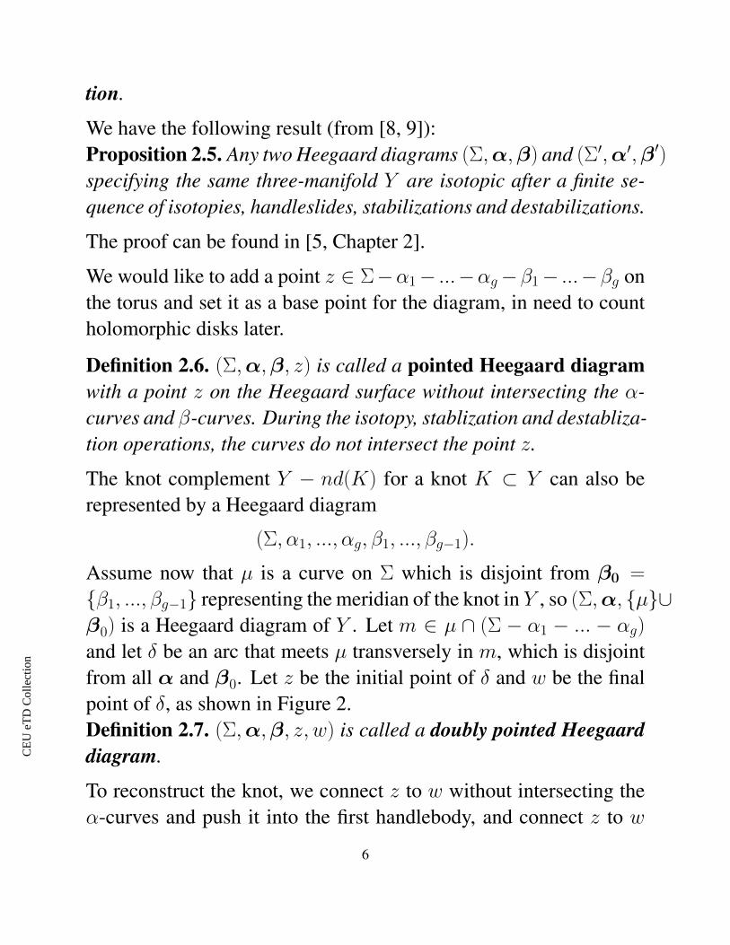
The homology of the associated graded object to CFK−(S3, K),that is, the same module equipped with the differential

∂−Kx =∑

y∈Tα∩Tβ

∑{φ∈π2(x,y)|µ(φ)=1,nz(φ)=0}

#M(φ)Unw(φ) · y.

which respects the Alexander filtration, provides, through taking ho-mology, the invariant the knot Floer homology group of K:

HFK−(S3, K) = H∗(CFK−(S3, K), ∂−K).

Considering the differential ∂−K induces on the quotinet complexCFK(S3, K) we get

∂Kx =∑

y∈Tα∩Tβ

∑{φ∈π2(x,y)|µ(φ)=1,nz(φ)=nw(φ)=0}

#M(φ) · y.

The corresponding homology is denoted by HFK(S3, K).

Obviously there exist exact sequences relating these chain complexes.The natural short exact sequences of chain complexes below inducelong exact sequences on their homologies.

0 −→ CFK−i−→ CFK∞ −→ CFK+ −→ 0

0 −→ CFKi−→ CFK+ U−→ CFK+ −→ 0,

here i is the inclusion map.

Following Theorem 4.8, we get the corollary below.Corollary 4.11. The knot homology groupsHFK+(S3, K), HFK(S3, K)

and HFK−(S3, K) are topological invariants for the knot K ⊂ S3,meaning that for two knots K1 and K2 in S3, if any of these threegroups corresponding to the two knots are different, then the knotK1 is not equivalent to K2.

21

CE

UeT

DC

olle

ctio

n

5 Genus-1 Heegaard diagram and the chain complex

In this section we will focus on applying the concepts of the previoussection to a genus-1 doubly pointed Heegaard diagram for a knot K.In this case, Σ = T is the torus, Symg(Σ) = T , α = {α1} andβ = {β1}, Tα = α1 and Tβ = β1. The chain group CFK∞(S3, K)

is generated by points from Tα ∩ Tβ = α1 ∩ β1.

If we choose two points x,y from Tα ∩ Tβ = α1 ∩ β1, we claim:

Theorem 5.1. For Heegaard diagram on torus T , the holomorphicdisks connecting x and y are the bigons on T connecting x and ywith boundary on the α1 and β1 curve. For each bigon φ ∈ π2(x,y),M(φ) = {pt}.Before the proof, we give a lemma which is needed.

Lemma 5.2. The Mobius transformations preserving the unit disk Din C are precisely those of the form

T (z) = λz − aaz − 1

,

where |λ| = 1 and |a| < 1. Denote the set of Mobius transformationsof this form by A = Aut(D).

Proof of Theorem 5.1. We consider the universal cover of T , whichis the complex plane C with the covering map π : C −→ T . Thelift of α1 and β1 are π−1(α1) and π−1(β1), they are embedded sub-manifold of C and each of them is homeomorphic to R × Z. Thebigons in T are lifted to bigons in C, for one bigon B ⊂ T , its liftπ−1(B) contains infinitely many bigons in C. Since each bigon is a

22

CE

UeT

DC

olle

ctio

n

simply connected subset in the complex plane, according to the Rie-mann mapping theorem, for one bigon B ⊂ π−1(B), we can find aholomorphic map f : D −→ B, where D is a unit disk in the com-plex plane. Combining this with the projection map we get a mapπ ◦ f : D −→ B from the unit disk to the bigon in T , and it is also aholomorphic map.

We have already proved that M(φ) is not empty. Now we want toprove the second part, which says that up to an equivalence relation,i.e. Mobius transformation, for a given bigon φ connecting x and y,there is only one holomorphic disk in the moduli space of φ. Assumethe holomorphic map from unit disk D in the complex plane to φ isu, then u induces a trivial map in the fundamental group, since Dis simply connected. According to the lifting criterion for coveringspace, u can be lifted to a map u which maps D to one bigon φ in C,φ ⊂ π−1(φ), and C is the universal cover of T . If there is anotherholomorphic map v from D to φ, we can also lift it to v which mapsD to φ. Since u and v are both bijective maps, they are actuallybiholomorphic. Combining v−1 with uwe get g = v−1◦u : D −→ D,and g(−i) = −i; g(i) = i. According to Lemma 5.2 and after somecomputation we get that a Mobius map from D to D preserving i and−i has the form

Ty(z) =z − iy1 + iy

,

where y can be any real number. This implies that u = v ◦ Ty.From this we know any two holomorphic maps from D to φ differby a Mobius map with the above form, hence dimM(φ) = 1 anddimM(φ) = 0, M(φ) = {pt}.

Now we know the differential map ∂∞ can be reduced to

23

CE

UeT

DC

olle

ctio

n

∂∞(x) =∑

y∈Tα∩Tβ

∑{φ∈π2(x,y)|µ(φ)=1}

Unw(φ)y.

We will discuss in detail about the property (∂∞)2 = 0 for the caseof genus-1 Heegaard diagram. To simplify matters, we notice thatwe can assume that the diagram contains only two bigons: one con-taining w and another one containing z. Indeed, if there is an emptybigon (i.e. one without w or z) then isotoping the β-curve we caneasily eliminate it. Continuing in this manner, we reach the casewhen we have two bigons.

Proposition 5.3. (∂∞)2 = 0.

Proof. We want to argue that for any x ∈ Tα∩Tβ, (∂∞)2(x) = 0. Theidea is that if we can find a bigonD1 connecting x and y, and a bigonD2 connecting y and u, then we can find a point v ∈ Tα ∩ Tβ with abigon D′1 connecting x and v, and a bigon D′2 connecting v and u insuch a way thatD1+D2 = D′1+D′2. Therefore a is counted two timesin (∂∞)2(x), so it becomes zero. There are mainly three cases, wewill use ∂ to represent ∂∞ and omit to count multiplicities of z andwin computation for convenience. (Indeed, since D1 +D2 = D′1 +D′2,the two count give coinciding results.)

In the first case, there are four bigons, D1 = φ1 + φ2, D2 = φ3.D1 connects x and y, D2 connects y and v, we find D′1 = φ1 + φ3

connecting x and u and D′2 = φ2 connecting u and v, see Figure 5.So we do the computation:

24

CE

UeT

DC

olle

ctio

n

Figure 10: Case 1

∂x = u + y + · · ·∂u = v + · · ·∂v = 0 + · · ·∂y = v + · · ·.

Thus, we get

∂2x = ∂(u + y) + · · · = 2v = 0 + · · ·.

For the second case, the bigon D1 = φ1 + φ3 + φ5 connect x to y,D2 = φ2 +φ4 connect y to u. We can find D′1 = φ1 +φ2 +φ3 connectx to t and D′2 = φ4 + φ5 connect t to u. So u appear twice in ∂2,which equals zero.

∂x = y + t + · · ·∂y = u + · · ·∂t = u + · · ·.

25

CE

UeT

DC

olle

ctio

n

Figure 11: Case 2

It is not hard to verify ∂2 = 0.

For the third case, D1 = φ1 + φ2 connect x to y, D2 = φ3 connect yto v, then D′1 = φ2 + φ3 connect x to u, D′2 = φ1 connect u to v. vappears twice in ∂2x, so it equals zero. We have the computation:

∂x = y + u + · · ·∂y = v + · · ·∂v = 0 + · · ·∂u = v + · · ·.

So that (∂∞)2 = 0.

Claim 5.4. ∂ = 0 for genus-1 doubly pointed Heegaard diagram.

Proof. As mentioned in the above proof, for any bigon which doesnot contain w and z, we can isotope the curves to eliminate suchbigon, so the bigons which remain contain at least one of the base-points. From the definition of ∂ we know it is equal to zero.

26

CE

UeT

DC

olle

ctio

n

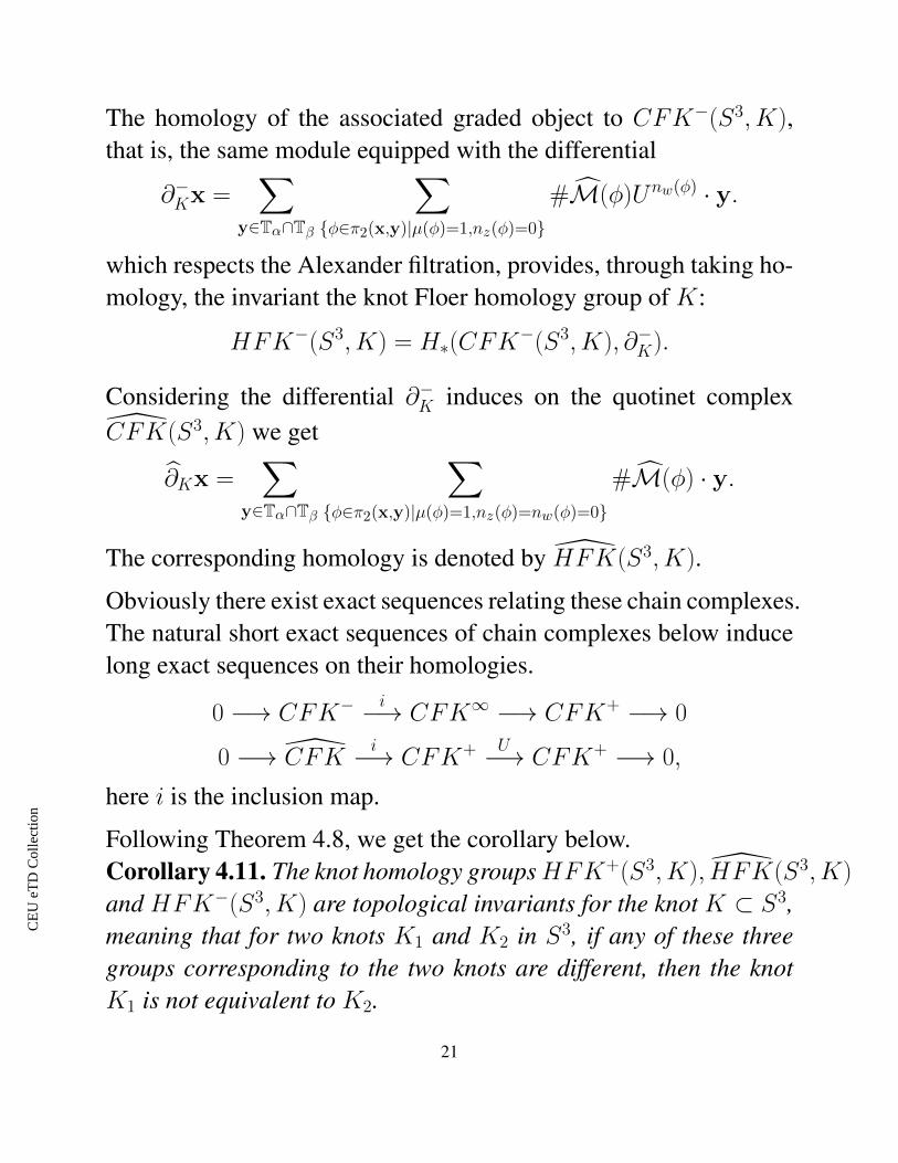
Figure 12: Case 3

6 Some Computations

In this section we will define the Alexander grading and the Maslovgrading, and will compute knot Floer homology for the trefoil knotand for the (-3,4)-torus knot with the doubly pointed Heegaard dia-gram given above, following the method used in [6, Chapter 6] [3,Chapter 3]. Since ∂− and ∂∞ gives the same computation, we willwrite ∂− here representing the two differentials.

6.1 Alexander grading and Maslov grading

Definition 6.1. For a given intersection point x ∈ Tα ∩ Tβ, theAlexander grading and Maslov grading are integers associated tox. We denote them to be A(x) and M(x). For any points x,y ∈Tα ∩ Tβ and φ ∈ π2(x,y), they satisfy the following formula:

M(x)−M(y) = µ(φ)− 2nw(φ) (1)

27

CE

UeT

DC

olle

ctio

n

A(x)− A(y) = nz(φ)− nw(φ) (2)

∑x∈Tα∩Tβ

(−1)M(x)qA(x) = ∆K(q). (3)

In Equation (3) ∆K is the Alexander-Conway polynomial of the knotK.

6.2 The trefoil knot

We have already obtained the doubly pointed Heegaard diagram forthe trefoil knot as show in Figure 3. Now we cut along the β-curveand a meridian curve of the torus which does not intersect the α-curve, and convert this diagram into a diagram on a square, as shownin Figure 6.2.

So the α and β curves intersect at three points x1, x2, x3, and thereare two bigons φ and ψ, φ connects x2 and x3, ψ connects x2 and x1.The boundary of these two bigons both have two parts, one part ison the α curve, the other part is on β curve. There exist holomorphicmaps from D to φ and ψ. The bigon from x2 to x3 contains z, whilethe bigon from x2 to x1 contains w. Therefore the differential ∂−

vanishes on x1 and x3 and ∂−x2 = x3 + Ux1. On the other hand,since the Alexander gradings of x2 and x3 are different (but A(x2) =

A(Ux1)), for the differential ∂−K of the associated graded object wehave

∂−Kx2 = Ux1.

28

CE

UeT

DC

olle

ctio

n

Figure 13: Plane Heegaard diagram for trefoil knot

29

CE

UeT

DC

olle

ctio

n

CFK∞(S3, K) is generated by x1, x2, x3 over Z2[U ]. If we con-sider CFK(S3, K), the generators are still x1, x2, x3 and the differ-ential ∂ = 0. So they also form generators of HFK(S3, K). We getHFK(S3, K) = Z3

2.

The homology HFK−(S3, K) for the trefoil knot K can be easilycomputed:

HFK−(S3, K) = Z2[U ]⊕ Z2

where Z2[U ] is generated by x3 and Z2 = Z2[U ]/UZ2[U ] is generatedby x1 (and Ux1 is zero in homology, since it is the boundary of x2).

6.3 (-3,4)-torus knot

From Section 2 we have already obtained the Heegaard diagram forthe (-3,4)-torus knot. We construct its universal cover, as shownbelow.

There is a holomorphic disk connecting x1 and x2 with one z pointinside, one holomorphic disk connecting x5 and x3 with two z pointinside, one disk connecting x5 and x2 with two w points inside, onedisk connecting x4 and x3 with one w points inside.

Using the earlier formulas for the gradings (1) and (2) we have:

30

CE

UeT

DC

olle

ctio

n

Figure 14: Universal cover for Heegaard diagram for trefoil knot

M(x1) = 6, A(x1) = 3,

M(x2) = 5, A(x2) = 2,

M(x3) = 2, A(x3) = 0,

M(x4) = 1, A(x4) = −2,

M(x5) = 0, A(x5) = −3.

It implies that

31

CE

UeT

DC

olle

ctio

n

∂−x1 = 0

∂−x2 = x1 + U 2x5

∂−x3 = Ux4 + x5

∂−x4 = 0

∂−x5 = 0

From this description the map ∂−K of the associated graded object canbe easily computed:

∂−Kx1 = 0

∂−Kx2 = U 2x5

∂−Kx3 = Ux4

∂−Kx4 = 0

∂−Kx5 = 0.

Therefore HFK(S3, K) for the (-3,4) torus knot K is isomorphic toZ5

2, while HFK−(S3, K) is isomorphic to Z2[U ]⊕ Z32, where Z2[U ]

is generated by x1, one copy of Z2 is generated by x4 (and it canbe viewed as Z2[U ]/UZ2[U ]), and the two further copies of Z2 aregenerated by x5 and Ux5 and as a Z2[U ]-module these two copies ofZ2 are equal to Z2[U ]/U 2Z2[U ].

32

CE

UeT

DC

olle

ctio

n

References

[1] H. Doll, A generalized bridge number for links in 3-manifolds, Math. Ann. Volume 294 , 701-717, 1992.

[2] A. Floer, A relative Morse index for the symplectic action,Comm. Pure Appl. Math., 41(4):393-407, 1988.

[3] H. Goda, H. Matsuda, T. Morifuji, Knot Floer homology of(1,1)-knots, Geometriae Dedicata, April 2005, Volume 112,Issue 1:197–214, 2005.

[4] M. Gromov, Pseudo-holomorphic curves in symplectic man-ifolds, Invent Math, Volume: 82, 307-348, 1985.

[5] P. Ozsvath, Z. Szabo, Holomorphic disks and topological in-variants for closed three-manifolds, Annals of Mathematics,Volume 159, Issue 3, 1027-1158, 2004.

[6] P. Ozsvath, Z. Szabo, Holomorphic disks and knot invari-ants, Advances in Mathematics, Volume 186, Issue 1, 58-116, 2004.

[7] J. Rasmussen, Knot Polynomials and Knot Homologies,arXiv:math/0504045.

[8] K. Reidemeister, Zur dreidimensionalen Topologie, Abh.Math. Sem. Univ. Hamburg, (9):189-194, 1933.

[9] J. Singer, Three-dimensional manifolds and their Heegaarddiagrams, Trans. Amer. Math Soc., 35(1):88-111, 1933.

33

CE

UeT

DC

olle

ctio

n