Embed Size (px)
Citation preview

SIMPLIFICATION OF COMBINATORIAL
LINK FLOER HOMOLOGY
ANNA BELIAKOVA
Abstract. We define a new combinatorial complex computing the hat version of
link Floer homology over Z/2Z, which turns out to be significantly smaller than
the Manolescu–Ozsvath–Sarkar one.
Introduction
Knot Floer homology is a powerful knot invariant constructed by Ozsvath–Szabo
[13] and Rasmussen [16]. In its basic form, the knot Floer homology HFK(K) of a
knot K ∈ S3 is a finite–dimensional bigraded vector space over F = Z/2Z
HFK(K) =⊕
d∈Z,i∈Z
HFKd(K, i) ,
where d is the Maslov and i is the Alexander grading. Its graded Euler characteristic∑
d,i
(−1)drank HFKd(K, i)ti = ∆K(t)
is equal to the symmetrized Alexander polynomial ∆K(t). The knot Floer homology
enjoys the following symmetry extending that of the Alexander polynomial.
(1) HFKd(K, i) = HFKd−2i(K,−i)
By the result of Ozsvath–Szabo [12], the maximal Alexander grading i, such
that HFK∗(K, i) 6= 0 is the Seifert genus g(K) of K. Moreover, Ghiggini showed
for g(K) = 1 [4] and Yi Ni in general [9], that the knot is fibered if and only if
rank HFK∗(K, g(K)) = 1. A concordance invariant bounding from below the slice
genus of the knot can also be extracted from knot Floer homology [11]. For torus
knots the bound is sharp, providing a new proof of the Milnor conjecture. The first
purely combinatorial proof of the Milnor conjecture was given by Rasmussen in [17]
by using Khovanov homology [5].
2000 Mathematics Subject Classification: 57R58 (primary), 57M27 (secondary)
Key words and phrases. Heegaard Floer homology, link invariants, fibered knot, Seifert genus.1

2 ANNA BELIAKOVA
−1−1
−1
−3
−2
−1
−2
Figure 1. A rectangular diagram for 52 knot. The number
associated to a domain is minus the winding number for its points.
The sets X and O consist of black and white points, respectively.
Knot Floer homology was extended to links in [15]. The first combinatorial con-
struction of the link Floer homology was given in [7] over F and then in [8] over Z.
Both constructions use grid diagrams of links.
A grid diagram is a square grid on the plane with n × n squares. Each square
is decorated either with an X, an O, or nothing. Moreover, every row and every
column contains exactly one X and one O. The number n is called complexity of
the diagram. Following [8], we denote the set of all O’s and X’s by O and X,
respectively.
Given a grid diagram, we construct an oriented, planar link projection by drawing
horizontal segments from the O’s to the X’s in each row, and vertical segments from
the X’s to the O’s in each column. We assume that at every intersection point the
vertical segment overpasses the horizontal one. This produces a planar rectangular
diagram G for an oriented link L in S3. Any link in S3 admits a rectangular diagram
(see e.g. [3]). An example is shown in Figure 1.
In [7], [8] the grid lies on the torus, obtained by gluing the top most segment of
the grid to the bottommost one and the leftmost segment to the right most one. In
the torus, the horizontal and vertical segments of the grid become circles. The MOS
complex is then generated by n–tuples of intersection points between horizontal and
vertical circles, such that exactly one point belongs to each horizontal (or vertical)
circle. Two generators x and y are connected by the differential if n− 2 points of x
and y coincide and if there exists a rectangle with vertices among x and y and edges
lying alternatively on horizontal and vertical circles, which does not contain X’s and

COMBINATORIAL LINK FLOER HOMOLOGY 3
Figure 2. Collection of short ovals for 52 knot. The dots show
a generator in Alexander grading 1.
O’s or points among x and y. The Alexander grading is given by formula (2) below,
and the Maslov grading by (3) plus one. The MOS complex has n! generators. This
number greatly exceeds the rank of its homology. For the trefoil, for example, the
number of generators is 120, while the rank of HFK(31) is 3.
In this paper, we construct another combinatorial complex computing link Floer
homology, which has significantly less generators. All knots with less than 6 crossings
admit rectangular diagrams where all differentials in our complex are zero, and the
rank of the homology group is equal to the number of generators.
Main results. Our construction also uses rectangular diagrams. Given an oriented
link L in S3, let G be its rectangular diagram in R2. Let us draw 2n − 2 narrow
short ovals around all but one horizontal and all but one vertical segments of the
rectangular diagram G in such a way, that the outside domain has at least one X
or O. We denote by S the set of unordered (n − 1)–tuples of intersection points
between the horizontal and vertical ovals, such that exactly one point belongs to
each horizontal (or vertical) oval. We assume throughout this paper that the ovals
intersect transversally. An example is shown in Figure 2.
A chain complex (C(G), ∂) computing the hat version of link Floer homology of L
over F = Z/2Z is defined as follows. The generators are elements of S. The bigrading
on S can be constructed analogously to those in [7]. Suppose ℓ is the number of
components of L. Then the Alexander grading is a function A : S −→ (12Z)ℓ, defined
as follows.

4 ANNA BELIAKOVA
Figure 3. The complex (C(G), ∂) with long ovals.
First, we define a function a : S → Zℓ. For a point p, the ith component of a is
minus the winding number of the projection of the ith component of the oriented
link around p. In the grid diagram, we have 2n distinguished squares containing X’s
or O’s. Let {ci,j}, i ∈ {1, . . . , 2n}, j ∈ {1, . . . , 4}, be the vertices of these squares.
Given x ∈ S, we set
(2) A(x) =∑
x∈x
a(x) −1
8
(∑
i,j
a(ci,j))−
(n1 − 1
2, . . . ,
nℓ − 1
2
),
where here ni is the complexity of the ith component of L, i.e. the number of
horizontal segments belonging to this component.
The homological or Maslov grading is a function M : S → Z defined as follows.
Given two collections A, B of finitely many points in the plane, let I(A, B) be the
number of pairs (a1, a2) ∈ A and (b1, b2) ∈ B with a1 < b1 and a2 < b2. Define
(3) M(x) = I(x,x) − I(x, O) − I(O,x) + I(O, O).
The differential in our complex is defined as follows. We first consider the link
Floer homology complex (C(S2, α, β, X, O), ∂) of Ozsvath–Szabo with extra base-
points X and O (the definition is recalled in Section 1). We assume that α and
β are 2(n − 1) long ovals (as long as n × n grid) encircling all but one horizontal
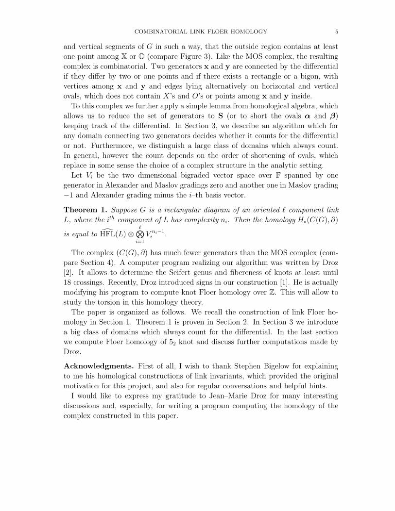
COMBINATORIAL LINK FLOER HOMOLOGY 5
and vertical segments of G in such a way, that the outside region contains at least
one point among X or O (compare Figure 3). Like the MOS complex, the resulting
complex is combinatorial. Two generators x and y are connected by the differential
if they differ by two or one points and if there exists a rectangle or a bigon, with
vertices among x and y and edges lying alternatively on horizontal and vertical
ovals, which does not contain X’s and O’s or points among x and y inside.
To this complex we further apply a simple lemma from homological algebra, which
allows us to reduce the set of generators to S (or to short the ovals α and β)
keeping track of the differential. In Section 3, we describe an algorithm which for
any domain connecting two generators decides whether it counts for the differential
or not. Furthermore, we distinguish a large class of domains which always count.
In general, however the count depends on the order of shortening of ovals, which
replace in some sense the choice of a complex structure in the analytic setting.
Let Vi be the two dimensional bigraded vector space over F spanned by one
generator in Alexander and Maslov gradings zero and another one in Maslov grading
−1 and Alexander grading minus the i–th basis vector.
Theorem 1. Suppose G is a rectangular diagram of an oriented ℓ component link
L, where the ith component of L has complexity ni. Then the homology H∗(C(G), ∂)
is equal to HFL(L) ⊗ℓ⊗
i=1
V ni−1i .
The complex (C(G), ∂) has much fewer generators than the MOS complex (com-
pare Section 4). A computer program realizing our algorithm was written by Droz
[2]. It allows to determine the Seifert genus and fibereness of knots at least until
18 crossings. Recently, Droz introduced signs in our construction [1]. He is actually
modifying his program to compute knot Floer homology over Z. This will allow to
study the torsion in this homology theory.
The paper is organized as follows. We recall the construction of link Floer ho-
mology in Section 1. Theorem 1 is proven in Section 2. In Section 3 we introduce
a big class of domains which always count for the differential. In the last section
we compute Floer homology of 52 knot and discuss further computations made by
Droz.
Acknowledgments. First of all, I wish to thank Stephen Bigelow for explaining
to me his homological constructions of link invariants, which provided the original
motivation for this project, and also for regular conversations and helpful hints.
I would like to express my gratitude to Jean–Marie Droz for many interesting
discussions and, especially, for writing a program computing the homology of the
complex constructed in this paper.

6 ANNA BELIAKOVA
I profited a lot from discussions with Stephan Wehrli. A special thank goes to
Ciprian Manolescu for sharing his knowledge of Heegaard Floer homology and for
his valuable suggestions after reading the preliminary version of this paper.
1. Link Floer homology with multiple basepoints
For the readers convenience, we review here the Ozsvath–Szabo construction of
knot and link Floer homologies, considering the case where the link meets the Hee-
gaard surface in extra intersection points. Our exposition follows closely [7, Section
2].
Let (Σ, α, β,w, z) be a Heegaard diagram for S3, where Σ is a surface of genus
g, k is some positive integer, α = {α1, ..., αg+k−1} are pairwise disjoint, embedded
curves in Σ which span a half–dimensional subspace of H1(Σ; Z) (and hence specify a
handlebody Uα with boundary equal to Σ), β = {β1, ..., βg+k−1} is another collection
of attaching circles specifying Uβ, and w = {w1, ..., wk} and z = {z1, ..., zk} are
distinct marked points with
w, z ⊂ Σ − α − β.
Let {Ai}ki=1 resp. {Bi}
ki=1 be the connected components of Σ − α resp. Σ − β.
We suppose that our basepoints are placed in such a manner that each component
Ai or Bi contains exactly one basepoint among the w and exactly one basepoint
among the z. We can label our basepoints so that Ai contains zi and wi, and then
Bi contains wi and zν(i), for some permutation ν of {1, ..., k}.
In this case, the basepoints uniquely specify an oriented link L in S3 = Uα ∪ Uβ ,
by the following conventions. For each i = 1, ..., k, let ξi denote the arc in Ai from zi
to wi and let ηi denote the arc in Bi from wi to zν(i). Let ξi ⊂ Uα be an arc obtained
by pushing the interior of ξi into Uα, and ηi be the arc obtained by pushing the
interior of ηi into Uβ. Now, we can let L be the oriented link obtained as the union
k⋃
i=1
(ξi + ηi
).
Definition 1.1. In the above case, we say that (Σ, α, β,w, z) is a 2k–pointed Hee-
gaard diagram compatible with the oriented link L in S3.
Let ℓ denote the number of components of L. Clearly, k ≥ ℓ. In the case where k =
ℓ, these are the Heegaard diagrams used in the definition of link Floer homology [15],
see also [13], [16]. In the case where k > ℓ, these Heegaard diagrams can still be
used to calculate link Floer homology, in a suitable sense.

COMBINATORIAL LINK FLOER HOMOLOGY 7
Definition 1.2. A periodic domain is a two–chain of the form
P =
k∑
i=1
(ai · Ai + bi · Bi)
such that wi /∈ P for all i. A Heegaard diagram is said to be admissible if for every
non–trivial periodic domain, the set {ai, bi} contains some stricktly positive and
negative numbers.
For simplicity, we consider now the case where L is a knot. The case of links can
be handled with a few minor notational changes in Subsection 1.1 below.
Let (Σ, α, β,w, z) be a Heegaard diagram compatible with an oriented knot K.
Let us consider the complex C(Σ, α, β,w, z) generated over F by intersection points
between tori Tα = α1 × · · · × αg+k−1 and Tβ = β1 × · · · × βg+k−1 in Symg+k−1(Σ)
endowed with the differential
(4) ∂x =∑
y∈Tα∩Tβ
∑
{φ∈π2(x,y)
∣∣ M(φ) = 1,
nwi(φ) = nzi
(φ) = 0 ∀i = 1, ..., k}
#
(M(φ)
R
)· y.
where π2(x,y) denotes the space of homology classes of Whitney disks (domains)
connecting x to y, M(φ) is the Maslov index of φ, np(φ) denotes the local multiplicity
of φ at the reference point p (i.e. the algebraic intersection number of φ with the
subvariety {p} × Symg+k−2(Σ)), M(φ) is the moduli space of pseudo–holomorphic
representatives of φ, and #() denotes a count modulo two. In the case when the
Heegaard diagram is admissible, the sum in Equation (4) is finite. We refer to [14]
for further details.
The relative Alexander grading of two intersection points x and y is defined by
the formula
A(x) − A(y) =
(k∑
i=1
nzi(φ)
)−
(k∑
i=1
nwi(φ)
).
The absolut A–grading can be fixed by requiring∑
x∈Tα∩Tβ
tA(x) ≡ ∆K(t) · (1 − t−1)k−1 (mod 2),
where ∆K(t) is the symmetrized Alexander polynomial which could be made to work
over Z by introducing signs.
Moreover, there is a relative Maslov grading, defined by
(5) M(x) − M(y) = M(φ) − 2
k∑
i=1
nwi(φ).

8 ANNA BELIAKOVA
The relative Maslov grading can also be lifted to an absolute grading as explained
in e.g. [7].
For this complex, the function A defines an Alexander grading which is preserved
by the differential. The following proposition shows how to extract the usual knot
Floer homology from the above variants using multiple basepoints. The proof is
given in [7], compare also [15].
Proposition 1.1. Let (Σ, α, β,w, z) be a 2k–pointed admissible Heegaard diagram
compatible with a knot K. Then, we have an identification
(6) H∗(C(Σ, α, β,w, z), ∂) ∼= HFK(K) ⊗ V ⊗(k−1),
where V is the two–dimensional vector space spanned by two generators, one in
bigrading (−1,−1), another in bigrading (0, 0).
1.1. Modifications for links. Recall that knot Floer homology has a generaliza-
tion to the case of oriented links L. For an ℓ component oriented link L in S3, this
takes the form of a multi–graded theory
HFL(L) =⊕
d∈Z,h∈H
HFLd(L, h),
where H ∼= H1(S3 − L) ∼= Zℓ, with the latter isomorphism induced by an order-
ing of the link components. The Euler characteristic determines the multivariable
Alexander polynomial ∆L(t1, ..., tℓ) as follows.
χ(HFL(L)) =
{ ∏ℓi=1(t
1/2i − t
−1/2i ) ∆L(t1, ..., tℓ) ℓ > 1
∆L(t) ℓ = 1
We sketch now the changes to be made to the above discussion to define link Floer
homology for Heegaard diagrams with extra basepoints.
Suppose now that (Σ, α, β,w, z) is a Heegaard diagram compatible with an ori-
ented link L in the sense of Definition 1.1.
Let us label the basepoints keeping track of which link component they belong
to. Specifically, suppose L is a link with ℓ components, and for i = 1, ..., ℓ, ni is the
number of pairs of basepoints on the ith component. Letting S be the index set of
pairs (i, j) with i = 1, ..., ℓ and j = 1, ..., ni. We now have basepoints {zi,j}(i,j)∈S
and {wi,j}(i,j)∈S.
We can now form the chain complex C(Σ, α, β,w, z) over F analogous to the
version before, generated by intersection points of Tα ∩ Tβ . This complex has a
relative Maslov grading as before. It also has an Alexander grading which in this

COMBINATORIAL LINK FLOER HOMOLOGY 9
case is an ℓ–tuple of integers,
A : Tα ∩ Tβ −→
(1
2Z
)ℓ
,
determined up to an overall additive constant by the formula
A(x) − A(y) =
(n1∑
j=1
(nz1,j(φ) − nw1,j
(φ)), ...,
nℓ∑
j=1
(nzℓ,j(φ) − nwℓ,j
(φ))
).
The indeterminacy in this case can be fixed with the help of Proposition 1.2.
The differential drops Maslov grading by one and preserves the Alexander multi–
grading, and hence the homology groups H∗(C(Σ, α, β,w, z)) inherit a Maslov grad-
ing and an Alexander multi–grading.
Proposition 1.2. Let (Σ, α, β,w, z) be a 2k–pointed admissible Heegaard diagram
compatible with an oriented link L, with ni pairs of basepoints corresponding to the
ith component of L. Then, there are multi–graded identifications
H∗(C(Σ, α, β,w, z), ∂) ∼= HFL(L) ⊗
ℓ⊗
i=1
V⊗(ni−1)i ,
where Vi is the two–dimensional vector space spanned by one generator in Maslov and
Alexander gradings zero, and another in Maslov grading −1 and Alexander grading
corresponding to minus the ith basis vector.
By the result of [15], the bigraded groups HFL(L) are link invariants. In partic-
ular, they do not change if
• the complex structure on Σ is varied;
• the α– and β–curves are moved by isotopies (in the complement of the
basepoints);
• the α– and β–curves are moved by handle–slides (in the complement of the
basepoints);
• the Heegaard diagram is stabilized.
1.2. MOS complex. It was shown in [7], that for a link of complexity n the MOS
complex, described in Introduction, coincides with the complex (C(Σ, α, β,w, z), ∂),
where Σ is a torus, α are n standard meridians on Σ, β are n standard longitudes
(both providing n × n grid on the torus), and where the basepoints w and z are
identified with X and O. Hence, by Proposition 1.2 the homology of this complex
is equal to HFL(L) ⊗⊗ℓ
i=1 V⊗(ni−1)i .

10 ANNA BELIAKOVA
x y
Figure 4. Removing of a bigon without basepoints inside.
2. The complex (C(G), ∂)
2.1. Shortening of ovals. Suppose G is a rectangular diagram of complexity n for
an oriented link L. Let (C, ∂) be the complex (C(S2, α, β, X, O), ∂), where α and
β are 2(n − 1) ovals encircling all but one horizontal and vertical segments of G,
respectively. It is easy to check that any periodic domain in this case has positive
and negative coefficients. The differential ∂ is given by counting of all Maslov index
one domains connecting two generators, which do not contain X’s and O’s and admit
holomorphic representatives.
The next lemma allows to “short” an oval by removing any bigon without base-
points inside (see Figure 4).
Lemma 2.1. Assume that α and β curves form a bigon with corners x and y
without basepoints inside. Then the complex (C, ∂) is homotopy equivalent to the
complex (C ′, ∂′) whose set of generators S(C ′) is obtained from S(C) by removing
all generators containing x or y.
Proof. Let us define the homotopy equivalence explicitly.
Let I : C ′ → C and P : C → C ′ be the obvious inclusion and projection. For any
x ∈ S(C), let h(x) be zero if y 6∈ x, otherwise h(x) is obtained from x by replacing
y by x. We define F : C → C ′ and G : C ′ → C as follows.
F = P (Id + ∂h) G = (Id + h∂)I
Here Id is the identity map. Then GF − Id = ∂h + h∂, i.e. GF is homotopic to the
identity on C. On the other hand, FG is the identity map on C ′.
Let us endow the complex C ′ with the differential ∂′ = F∂G. It is easy to
check that ∂′2 = 0 and that F and G are chain maps. Indeed, ∂′F = F∂IP and
IP∂G = G∂′, or ∂′F = F∂ and ∂G = G∂′ over F.
Let us describe the new differential ∂′ = P (∂ + ∂h∂)I in more details. Assume
y ∈ ∂x and x, y do not contain the corners of the bigon x and y. For all such x and
y, ∂ and ∂′ coincide, i.e. we have y ∈ ∂′x. Furthermore, assume a,b ∈ S(C) do not
contain x and y, then for any x,y ∈ S(C) with y ∈ y, x ∈ x, such that h(y) = x,
y ∈ ∂a, and b ∈ ∂x, b occurs once in ∂′a. �

COMBINATORIAL LINK FLOER HOMOLOGY 11
2.2. Definition of the complex (C(G), ∂). We define the complex (C(G), ∂) as
obtained from the complex with long ovals by applying Lemma 2.1 several times,
until the complex has S as the set of generators. This subsection aims to give a
recursive definition of the differential ∂ in this complex. In general, it will depend
on the order in which the ovals were shortened.
Given x,y ∈ S, there is an oriented closed curve γx,y composed of arcs belonging
to horizontal and vertical ovals, where each piece of a horizontal oval connects a
point in x to a point in y (and hence each piece of the vertical one goes from a
point in y to a point in x). In S2, there exists an oriented (immersed) domain Dx,y
bounded by γx,y. The points x and y are called corners of the domain Dx,y.
Let Di be the closures of the connected components of the complement of ovals
in S2. Suppose that the orientation of Di is induced by the orientation of S2. Then
we say that a domain D =∑
i niDi connects two generators if for all i, ni ≥ 0 and
D is connected. Let D be the set of all domains connecting two generators which
do not contain X and O inside.
We define
∂x :=∑
M(y)=M(x)−1
∑
Dx,y∈D
m(Dx,y) y ,
where M(x) is the Maslov grading defined by (3) and m(Dx,y) ∈ {0, 1} is a multi-
plicity of the domain. In what follows we give an algorithm which determines these
multiplicities.
Let us fix the order in which the ovals were shortened. For any domain Da,b ∈ D
we prolongate the last oval which was shortened to obtain this domain, and show
whether in the resulting complex (C ′(G), ∂′), one can find x and y with y ∈ ∂′a,
h(y) = x and b ∈ ∂′x as in the proof of Lemma 2.1. If there is an odd number of
such x and y, then m(Da,b) = 1, otherwise the multiplicity is zero. To determine
m(Da,y) and m(Dx,b) in the new complex, we prolongate the next oval, and continue
to do so until the domains in question are polygons which always count.
This process is illustrated in Figure 5, where a and b are given by black and
white points respectively; y is obtained from a by switching the black point on the
dashed oval to y and the upper black point to the white point on the same oval; x is
obtained from y by switching y to x. Here the algorithm terminates after the first
step.
In fact, the algorithm terminates already when the domains in question are
strongly indecomposable with nondegenerate system of cuts (as defined in the next
section) since they all count for the differential.

12 ANNA BELIAKOVA
x
y
Figure 5. Immersed polygon realizing a differential from
black to white points. The prolongated oval is shown by a dashed
line.
2.3. Proof of Theorem 1. By Lemma 2.1, the complex (C(G), ∂) is homotopy
equivalent to the complex with long ovals. Moreover, the Alexander and Maslov
gradings are fixed in such a way, that
χ(C(G), ∂) =
{ ∏ℓi=1 t
1/2i (1 − t−1)ni∆L(t1, ..., tℓ) ℓ > 1
(1 − t−1)ni−1∆L(t) ℓ = 1
This can be shown by comparing our and MOS complexes. Indeed, one can construct
a bijection identifing the bigraded generators of our and MOS complexes which do
not cancel on the level of the Euler characteristic (see [1] for more details).
Hence Proposition 1.2 computes the homology of our complex. �
3. Indecomposable domains
In this Section we introduce a large class of domains which always count for the
differential. Let us start with some definitions.
3.1. Maslov index. Let e(S) be the Euler measure of a surface S, which for any
surface S with k acute right–angled corners, l obtuse ones, and Euler characteristic
χ(S) is equal to χ(S) − k/4 + l/4. Moreover, the Euler measure is additive under
disjoint unions and gluings along boundaries. In [6, Section 4], Lipshitz give a
formula computing the Maslov index M(Dx,y) of Dx,y as follows.
(7) M(Dx,y) = e(Dx,y) + nx + ny ,
where nx =∑
x∈x nx. The number nx is the local multiplicity of the domain at the
corner x, e.g. nx = 0 for an isolated corner , nx = 1/4 for an acute (or π/2–angled)
corner, nx = 1/2 for a straight (or π–angled) corner or nx = 3/4 for an obtuse (or

COMBINATORIAL LINK FLOER HOMOLOGY 13
Figure 6. Indecomposable, but not strongly indecomposable domain.
The oval destroying the indecomposability is shown by the dashed line.
3π/2–angled) one. For a composition of two domains Dx,z = Dx,y ◦ Dy,z, we have
M(Dx,z) = M(Dx,y) + M(Dy,z).
A domain D is called decomposable if it is a composition of Maslov index zero
and one domains; otherwise, the domain is indecomposable. A domain is called
strongly indecomposable if it is indecomposable and no prolongations of ovals inside
this domain destroy its indecomposability. An example of an indecomposable, but
not strongly indecomposable domain is shown in Figure 6.
3.2. Count of domains. In what follows any domain is assumed to belong to D, i.e.
to have Maslov index one and no basepoints inside, and to connect two generators.
We will also assume that our domains have no corners with negative multiplicities
or with multiplicities bigger than 3/4, since such domains never count (which can
easily be seen by applying the algorithm from the previous section).
A path in a domain starting at an obtuse or straight corner and following a
horizontal or vertical oval until the boundary of the domain will be called a cut.
There are two cuts at any obtuse corner and one at any straight corner.
We say that a cut touches a boundary component A at an oval B if either the
end point of this cut belongs to B or the cut is a prolongation of B. We define
the distance between two cuts touching A to be odd, if one of them touches A at a
vertical oval and another one at a horizontal oval; otherwise the distance is even.
A system of cuts in a domain is called degenerate if there is a boundary component
such that all cuts touching this component have an even distance to each other;
otherwise, the system of cuts is called nondegenerate. An example of a degenerate
system of cuts is given in Figure 7. Since two cuts (a horizontal and a vertical one)
leave any obtuse corner, a system of cuts can be degenerate only if our domain has

14 ANNA BELIAKOVA
Figure 7. An indecomposable domain with a degenerate sys-
tem of cuts.
at least one inner boundary component without obtuse corners. Let us call such an
inner boundary component bad.
Theorem 3.1. Any strongly indecomposable domain with a nondegenerate system
of cuts counts for the differential.
Corollary 3.2. Any strongly indecomposable domain without bad components counts
for the differential.
Proof. The proof is by induction on the number of boundary components c in the
domain. If c = 1, it is easy to see by prolongating ovals that any immersed polygon
counts.
Assume that for c = n − 1, the claim holds. Suppose our complex has a strongly
indecomposable domain D ∈ D with a nondegenerate system of cuts and n boundary
components. Examples with c = 2 are drawn in Figure 8.
Let us stretch one oval in D. Then D gives rise to a domain D′ with c = n − 1
boundary components. (Prolongations splitting one boundary component into two
are considered as immersions.) Let x and y be the corners of the bigon, obtained
after stretching. The stretched oval connects y to some boundary component, say
A. By Lemma 3.4 below, y can also be connected with A by a unique path inside
D. This path do not intersect the prolongated part, since our domain is strongly in-
decomposable. Hence, D′ can be represented as a union of two domains connecting
some generators. The unique path connecting y with A leaves any boundary com-
ponent along a cut. Moreover, if the path goes along the boundary of a component
without obtuse corners, then it also meets a component with two obtuse corners
(compare Proof of Lemma 3.4). Therefore, D′ is a union of two strongly indecom-
posable Maslov index one domains with nondegenerate system of cuts, which count
for the differential by the induction hypothesis. Applying Lemma 2.1, we conclude
that the domain D also counts for the differential.

COMBINATORIAL LINK FLOER HOMOLOGY 15
x
y
x y
Figure 8. Strongly indecomposable domains realizing differ-
entials from black to white points. The prolongated oval is shown
by a dashed line.
�
3.3. Structure of domains. Here we provide some technical results needed for the
proof of Theorem 3.1.
Definition 3.3. A boundary component C1 ⊂ ∂Dx,y is called y–connected with
another component C2 ⊂ ∂Dx,y if for any point y ∈ C1 disjoint from the corners,
there exists a unique path starting at y and ending in C2, such that
1) the path goes along cuts or ∂Dx,y, where the segments of horizontal and vertical
ovals alternate along the path;
2) the corners of the path (i.e. intersection points of horizontal and vertical
segments) come alternatively from x and y, where y contains y and intersection
points of cuts with ∂Dx,y;
3) the first corner belongs to x.
Lemma 3.4. In an indecomposable domain with a nondegenerate system of cuts,
any two boundary components are y–connected.
Proof. Recall that an inner boundary component without obtuse corners is called
bad. Let b be the number of bad components and c be the total number of boundary
components in our domain. Assume first that the domain has no straight corners.
In this case, we prove the claim by induction on c and b.
Assume b = 0, c = 2. If one of the cuts goes from the inner boundary component
to itself, the domain is decomposable (see Figure 9 (a)). If it is not the case, then
an easy check verifies the claim (compare Figure 9 (b)).

16 ANNA BELIAKOVA
x y
xy
y x
x y
y
y
a) b)
Figure 9. Case b = 0, c = 2. a) Decomposable domain. The cuts
are shown by dashed lines. b) Indecomposable domain. The corners
from x are marked by x and the points from y by y.
C
A
y
y
y y x
x
x y
yy
xx
C
A
y
y
y y
x
x
x
x y
yy
x
Figure 10. C is y–connected to A. The two choices of y are shown
by red and blue dots. The connected paths have the corresponding
colors. All corners without cuts are assumed to be acute.
Assume the claim holds for b = 0, c = n−1. Let us add an n–th good component
A to the domain. Then if there are no cuts ending at A, we are done, since two
cuts from the obtuse corner y–connect A to any other component by the induction
hypothesis.
If there is a component connected with A by two cuts, then it is y–connected
with the outside exactly in the case when A has this property. To check this, it is
sufficient to find a required path for two choices of y (before and after one corner)
on this component. An example is shown in Figure 10. Note that the particular
form of the domain does not matter for the argument.
If all cuts ending at A come from components connected with A by two cuts (as in
Figure 10), then A is y–connected to the outside by the previous argument. Suppose
there is a component C ⊂ ∂Dx,y connected with A by just one cut (see Figure 11).

COMBINATORIAL LINK FLOER HOMOLOGY 17
AC
Figure 11. C is connected to A by one cut. All corners without
cuts are assumed to be acute.
A
C
A
C
a) b)
Figure 12. Case b = 0, c = n. a) Decomposable domain. b)
Indecomposable domain, the system of cuts is nondegenerate.
Then there are two possibilities: either the path described in Definition 3.3 after
leaving A (along one of the cuts) comes back throught C without visiting all other
components or it does not happens. In the first case, the domain is decomposable,
since the path can be used to split the domain. In the second case, all components
are y–connected.
The case when C and A exchange two cuts is similar: either the domain is de-
composable or all components are y–connected (compare Figure 12). If C and A
exchange three or more cuts, the domain is decomposable.
Assume b = 1, c = n. Let us denote by B the bad component. Then, since
M(Dx,y) = 1, either the outer boundary component has an obtuse corner or an
inner boundary component E ⊂ ∂Dx,y has two obtuse corners. In the first case,
both cuts from the obtuse corner on the outer component should end at B, otherwise
the system of cuts is degenerate or the domain is decomposable.
Let us consider the second case. If B is not connected with ∂Dx,y by a cut, the
domain is decomposable. If there are three cuts connecting E with B or connecting
E with ∂Dx,y \ B, then the domain is decomposable again.

18 ANNA BELIAKOVA
E
B
Figure 13. Case b = 1, c = n. All drawn components are y–
connected. All corners without cuts are assumed to be acute.
If there are two paths connecting E with B (or with ∂Dx,y \B), such that each of
them leaves E at a different obtuse corner, then the domain is either decomposable
or have a degenerate system of cuts.
Hence, in our case, two cuts from one obtuse corner of E should connect E
with components, say A1, . . . , Ak, which are otherwise not connected with B, and
two cuts from the other obtuse corner should connect E with B. Therefore, the
situation looks like in Figure 13, where all components are y–connected.
If there are components connected with B by one or two cuts, they are also
y–connected with the remaining components, since B is y–connected with them.
The case b = k, c = n is similar. Again 2k cuts should be absorbed by bad
components. If a bad component is touched by no pair of cuts at odd distance, the
system of cuts is degenerate; otherwise the component is y–connected to the outside
or the domain is decomposable.
It remains to consider the case where Dx,y has straight corners. In this case, one
of the boundary components is an oval with a common corner of two generators.
Let us call such a component special. An example is shown in Figure 8. Let us first
assume that we have only one special component. Then the cut from the straight
corner y–connects this component with any other one (otherwise not connected with
the special one) by the previous argument. If we have a component connected with
the special one by one or two cuts, then it is also y–connected with all the others,
since the special component has this property. The obvious induction completes the

COMBINATORIAL LINK FLOER HOMOLOGY 19
0
−1
1−1
10
Figure 14. A complex for 52 knot. The colored dots show genera-
tors in the maximal Alexander grading equal to 1. A number assigned
to a region is minus the winding number for its points.
proof. Note that if two (or more) special components exchange their cuts, then the
domain is decomposable. �
4. Computations
In this section we show how HFK of small knots can be computed by hands and
discuss the computer program written by Droz.
4.1. 52 knot. Figure 14 shows a rectangular diagram for 52 knot of complexity n = 7
obtained from the original diagram in Figure 1 by cyclic permutations (compare [3]).
An advantage of this diagram is that there are no regions counted for the differential.
The Alexander grading of a generator is given by the formula A(x) =∑
x∈x a(x)−
2. The maximal Alexander grading is equal to one. There are two generators in this
grading shown by colored dots in Figure 14. Both of them have Maslov grading 2.
The homology of our complex is HFK(52)⊗V 6. Hence in Alexander grading zero,
we have 12 additional generators coming from the multiplication with V . Note that
our complex has 15 generators in Alexander grading zero. Indeed, 12 of them can be
obtained by moving one point of a generator in Alexander grading one to the other
side of the oval. In three cases, depicted by white dots there are two possibilities
to move a point. This gives 3 additional generators. Note that all movings drop

20 ANNA BELIAKOVA
Maslov index by one. We deduce that HFK(52, 0) has rank three. To compute HFK
in the negative Alexander gradings we use the symmetry (1).
Finally, we derive that HFK(52) has rank two in the Alexander–Maslov bigrading
(1, 2), rank three in (0, 1), and rank two in the bigrading (−1, 0). To compare, the
Alexander polynomial is ∆52(t) = 2(t + t−1) − 3. The knot 52 is not fibered and its
Seifert genus is one.
4.2. Droz’s program. Droz wrote a computer program calculating the homology
of our complex, which is already installed on the Bar–Natan’s Knot Atlas [2]. As
a byproduct, his program generates rectangular diagrams of knots and links and
allows to change them by Cromwell–Dynnikov moves. The program can be used
to determine Seifert genus and fibereness of knots at least until 18 crossings. The
precise description of the algorithm is given in [1], where Droz also introduces signs
in our construction.
According to Droz’s computations, the number of generators in our complex is
significantly smaller than that in the MOS complex. Moreover, for small knots,
almost all domains suitable for the differential are embedded polygons, so they
always count for the differential. For example, for knots admitting rectangular
diagrams of complexity 10, the number of generators in the MOS complex is 10! =
3′628′800. Our complex has on average about 50′000 generators among them about
1′000 in the positive Alexander gradings. The knot 12n2000 admits a rectangular
diagram of complexity 12, where 12! = 479′001′600. Our complex has 1′411′072
generators with 16′065 in the positive Alexander gradings.
References
[1] J.–M. Droz. Effective computation of knot Floer homology, in preparation.
[2] J.–M. Droz. Python program at http://www.math.unizh.ch/assistenten/jdroz or at
http://katlas.org/wiki/Heegaard Floer Knot Homology.
[3] I. Dynnikov. Arc–presentations of links: monotonic simplification. Fund. Math., 190:29–76,
2006.
[4] P. Ghiggini. Knot Floer homology detects genus-one fibred links. math.GT/0603445, 2006.
[5] M. Khovanov. A categorification of the Jones polynomial. Duke Math. J., 101(3):359–426,
2000.
[6] R. Lipshitz. A cylindrical reformulation of Heegaard Floer homology. math.SG/0502404, 2005.
[7] C. Manolescu, P. Ozsvath, S. Sarkar. A combinatorial description of knot Floer homology.
math.GT/0607691
[8] C. Manolescu, P. Ozsvath, Z. Szabo, D. Thurston. On combinatorial link Floer homology.
math.GT/0610559
[9] Y. Ni. Knot Floer homology detects fibred knots. math.GT/0607156.

COMBINATORIAL LINK FLOER HOMOLOGY 21
[10] P. S. Ozsvath and Z. Szabo. Heegaard Floer homology and alternating knots. Geom. Topol.,
7:225–254, 2003.
[11] P. S. Ozsvath and Z. Szabo. Knot Floer homology and the four–ball genus. Geom. Topol.,
7:615–639, 2003.
[12] P. S. Ozsvath and Z. Szabo. Holomorphic disks and genus bounds. Geom. Topol., 8:311–334,
2004.
[13] P. S. Ozsvath and Z. Szabo. Holomorphic disks and knot invariants. Adv. Math., 186(1):58–
116, 2004.
[14] P. S. Ozsvath and Z. Szabo. Holomorphic disks and topological invariants for closed three–
manifolds. Ann. of Math. (2), 159(3):1027–1158, 2004.
[15] P. S. Ozsvath and Z. Szabo. Holomorphic disks, link invariants, and the multi–variable Alexan-
der polynomial. math.GT/0512286, 2005.
[16] J. A. Rasmussen. Floer homology and knot complements. PhD thesis, Harvard University,
2003.
[17] J. A. Rasmussen. Khovanov homology and the slice genus. math.GT/0402131, 2004.
Institut fur Mathematik, Universitat Zurich, Winterthurerstrasse 190, CH-8057
Zurich, Switzerland
E-mail address : [email protected]


![Heegaard Floer homology of spatial graphsshelly/publications/HFG.pdf · Knot Floer homology, introduced by P Ozsváth and Z Szabó[18], and independently by J Rasmussen[20], is an](https://img.pdfslide.us/doc/110x75/5f0396a67e708231d409cb3e/heegaard-floer-homology-of-spatial-graphs-shellypublicationshfgpdf-knot-floer.jpg)