Embed Size (px)
Citation preview
8/3/2019 Robert Lipshitz- A Cylindrical Reformulation of Heegaard Floer Homology
http://slidepdf.com/reader/full/robert-lipshitz-a-cylindrical-reformulation-of-heegaard-floer-homology 1/135
ISSN numbers are printed here 1
A Cylindrical Reformulation of Heegaard Floer Homology
Robert Lipshitz
Stanford University, Stanford, CA 94305-2125 USA
Email: [email protected]
Abstract
We reformulate Heegaard Floer homology in terms of holomorphic curves in the cylindrical
manifold Σx[0, 1]xR, where Σ is the Heegaard surface, instead of Symg(Σ). We then showthat the entire invariance proof can be carried out in our setting. In the process, we derivea new formula for the index of the ∂ –operator in Heegaard Floer homology, and shortenseveral proofs. After proving invariance, we show that our construction is equivalent tothe original construction of Ozsvath–Szabo. We conclude with a discussion of elaborationsof Heegaard Floer homology suggested by our construction, as well as a brief discussion of the relation with a program of C. Taubes.
AMS Classification numbers Primary: 57R17
Secondary: 57R58; 57M27
Keywords: Heegaard–Floer homology, symplectic field theory, holomorphic curves, three–manifold invariants
Copyright declaration is printed here
8/3/2019 Robert Lipshitz- A Cylindrical Reformulation of Heegaard Floer Homology
http://slidepdf.com/reader/full/robert-lipshitz-a-cylindrical-reformulation-of-heegaard-floer-homology 2/135
2 Robert Lipshitz
In [21], P. Ozsvath and Z. Szabo associated to a three–manifold Y and a SpinC–structure
s on Y a collection of abelian groups, known together as Heegaard Floer homology. Thesegroups, which are believed to be isomorphic to certain Seiberg–Witten Floer homologygroups ([20], [12]), fit into the framework of a (3+1)–dimensional topological quantum fieldtheory. Since its discovery around the turn of the millennium, Heegaard Floer homologyhas been applied to the study of knots and surgery ([19], [25], [18], ...), contact structures([23]), and symplectic structures ([22]), and is strong enough to reprove most results aboutsmooth four–manifolds originally proved by gauge theory ([17]). In this paper we give analternate definition of the Heegaard Floer homology groups.
Rather than being associated directly to a three–manifold Y , the Heegaard Floer homologygroups defined in [21] and in this paper are associated to a Heegaard diagram for Y , as wellas a SpinC–structure s and some additional structure. A Heegaard diagram is a closed,
orientable surface Σ of genus g , together with two g –tuples of pairwise disjoint, homolog-ically linearly independent, simple closed curves α = α1, · · · , αg and β = β 1, · · · , β gin Σ . A Heegaard diagram specifies a three–manifold as follows. Thicken Σ to Σ × [0, 1].Glue thickened disks along the αi × 0 and along the β j × 1. The resulting space hastwo boundary components, each homeomorphic to S 2 . Cap each with a three–ball. Theresult is the three–manifold specified by (Σ, α, β ).
Different Heegaard diagrams can specify the same three–manifold. Two different Heegaarddiagrams specify the same three–manifold if and only if they agree after a sequence of moves of the following three kinds:
• Isotopies of the α– or β –circles.
• Handleslides among the α– or β –circles. These correspond to pulling one α– (orβ –) circle over another.
• Stabilization, which corresponds to taking the connect sum of the Heegaard diagramwith the standard genus–one Heegaard diagram for S 3 .
See [9, Sections 4.3 and 5.1] or [21, Section 2] for more details.
So, after associating the Heegaard Floer homology groups to a Heegaard diagram, one mustprove they are unchanged by these three kinds of Heegaard moves (as well as deforming theadditional structure involved in their definition). Doing so comprises most of [21] for theoriginal definition. Similarly, for our definition, most of this paper is involved in proving
Theorem 1 The Heegaard Floer homology groups HF ∞(Σ, α, β, s), HF +(Σ, α, β, s),
HF −(Σ, α, β, s) and HF (Σ, α, β, s) associated to a Heegaard diagram (Σ, α, β ) and SpinC– structure s are in fact invariants of the pair (Y, s).
We are also able to prove
Geometry & T opology , Volume X (20XX)
8/3/2019 Robert Lipshitz- A Cylindrical Reformulation of Heegaard Floer Homology
http://slidepdf.com/reader/full/robert-lipshitz-a-cylindrical-reformulation-of-heegaard-floer-homology 3/135
A Cylindrical Reformulation of Heegaard Floer Homology 3
Theorem 2 The Heegaard Floer homology groups defined in this paper are isomorphic
to the corresponding groups defined in [21].
Theorem 2 is proved in Section 13. The proof does not rely on the invariance results provedin this paper; it could be carried out immediately after Section 8. (We defer the proof tothe end to avoid interrupting the narrative flow.) Clearly, Theorem 2 implies Theorem 1.However, one key goal of this paper is to demonstrate that the entire invariance proof canbe carried out in our setting, and to develop the tools necessary to do so.
The only esentially new results in this paper are in Section 4, where we give a nice formulafor the index of the ∂ operator in our setup, and hence also the Maslov index in thetraditional setting, and in the discussion of elaborations of Heegaard Floer homology inthe last section (Section 14). The casual reader might also be interested in looking at the
elaboration and speculation in Section 14.
Although this paper is essentially self contained, it is probably most useful to read it inparallel with [21]. To facilitate this, the paper is organized similarly to [21], and throughoutthere are precise references to corresponding results in their original forms. In addition,the last appendix is a table cross referencing most of the results in this paper with thoseof [21].
A more technical discussion of the difference between our setup and that of [21] follows.
The original definition of Heegaard Floer homology involves holomorphic disks in Symg(Σ).In this paper, we consider holomorphic curves in Σ×[0, 1]×R. For instance, for us the chain
complex CF is generated by g–tuples of Reeb chords xi × [0, 1] | xi ∈ αi ∩ β σ(i)
. For anappropriate almost complex structure J on Σ × [0, 1] × R, the coefficient of yi × [0, 1]in ∂ (xi × [0, 1]) is given by counting holomorphic curves in Σ × [0, 1] ×R asymptotic toxi × [0, 1] at −∞ and to yi × [0, 1] at ∞, with boundary mapped to the Lagrangiancylinders α j ×1×R and β j ×0×R. (We impose a few further technical conditionson the curves that we count; see Section 1.)
If J is the split complex structure jΣ × jD then a holomorphic curve in Σ × [0, 1] ×R is justa surface S and a pair of holomorphic maps uΣ : (S,∂S ) → (Σ, α1 ∪ · · · ∪ αg ∪ β 1 ∪ · · · ∪ β g)and uD : (S,∂S ) → (D, ∂ D). If the map uD is a g –fold branched covering then this dataspecifies a map D → Symg(Σ) as follows. For p ∈ D, let p1, · · · , pg be the preiamgesof p under πD u, listed with multiplicity. Then the map D → Symg(Σ) sends p to
uΣ( p1), · · · , uΣ( pg).Note that the idea of viewing a map to Symg(Σ) as a pair
(a g–fold covering S → D, a map S → Σ)
is already implicit in [21], although they use this idea mainly for calculations in specialcases.
Geometry & T opology , Volume X (20XX)
8/3/2019 Robert Lipshitz- A Cylindrical Reformulation of Heegaard Floer Homology
http://slidepdf.com/reader/full/robert-lipshitz-a-cylindrical-reformulation-of-heegaard-floer-homology 4/135
4 Robert Lipshitz
Working in Σ × [0, 1] × R has several advantages. A main advantage is that, unlike a
g –fold symmetric product, one can actually visualize Σ × [0, 1] ×R. A second advantage isthat a number of the technical details become somewhat simpler. The main disadvantageis that we must now consider higher genus holomorphic curves, not just disks. Anotherdifficulty is that our setup requires compactness for holomorphic curves in manifolds withcylindrical ends, proved in [2]. I also borrow from the language of symplectic field theory.Fortunately, much of the subtle machinery of symplectic field theory, like virtual cycles orthe operator formalism, is unnecessary for this paper.
The paper is organized as follows. The first two sections are devoted to basic definitionsand notation, and certain algebro–topological considerations. The third section provestransversality results necessary for the rest of the paper. These results should be standard,but I am unaware of a reference that applies to our setting.
The fourth section discusses the index of the ∂ –operator in our context. We prove thisindex is the same as the Maslov index in the traditional setting, and obtain a combinatorialformula for it. The fifth section discusses so–called admissibility criteria necessary for thecase b1(Y ) > 0. The definitions and results are completely analogous with [21]. The sixthsection discusses coherent orientations of the moduli spaces. Again, our treatment is closeto [21].
The seventh section rules out undesirable codimension–one degenerations of our holomor-phic curves. After doing so, we are finally ready to define the Heegaard Floer chaincomplexes in Section 8, and turn to the invariance proof. The ninth section proves isotopyindependence. Before proving handleslide independence, we introduce triangle maps in
Section 10. (As in [21], to a Heegaard triple–diagram (Σ, α1, · · · , αg, β 1, · · · , β g, γ 1, · · · , γ g)is associated maps HF (Σ, α, β ) ⊗ HF (Σ, β, γ ) → HF (Σ, α, γ ), for various decorations of HF .) Using these triangle maps and a model computation, we prove handleslide invariancein Section 11.
Finally, in section twelve we prove stabilization invariance, completing the invariance proof.After this, we devote a section to proving equivalence with traditional Heegaard Floerhomology and a section to elaborations and speculation.
There are also two appendices. The first is devoted to the gluing results used throughoutthe paper. The second cross references our results with those in [21].
For technical results about holomorphic curves, this paper sometimes cites recent sources
when older ones would suffice. This generally reflects either that the newer results are morebroadly applicable or that I found the newer exposition significantly clearer.
I thank Ya. Eliashberg, who is responsible for communicating to me most of the ideas inthis paper. I also thank Z. Szabo for a helpful conversation about the index; P. Ozsvathfor a helpful conversation about annoying curves (see Section 8 below) and pointing out aserious omission in Section 13; P. Melvin for a stimulating conversation about the index; M.
Geometry & T opology , Volume X (20XX)
8/3/2019 Robert Lipshitz- A Cylindrical Reformulation of Heegaard Floer Homology
http://slidepdf.com/reader/full/robert-lipshitz-a-cylindrical-reformulation-of-heegaard-floer-homology 5/135
A Cylindrical Reformulation of Heegaard Floer Homology 5
Hutchings for a discussion clarifying the relation between the H 1(Y )–action and twisted
coefficients; M. Hedden and C. Wendl for pointing out errors, both typographical andotherwise, in a previous version; and W. Hsiang, C. Manolescu, L. Ng and B. Parker forcomments that have improved the exposition. Finally, I thank the referees for findingseveral errors and making many helpful suggestions.
This work was partially supported by the NSF Graduate Research Fellowship Program,and partly by the NSF Focused Research Group grant DMS–0244663.
1 Basic Definitions and Notation
By a pointed Heegaard diagram we mean a Heegaard diagram (as discussed in the intro-
duction) together with a chosen point z of the Heegaard surface in the complement of the α– and β –circles. Fix a p ointed Heegaard diagram H = (Σg, α = α1, · · · , αg, β =β 1, · · · , β g, z). Let α = α1 ∪ · · · ∪ αg ⊂ Σ and β = β 1 ∪ · · · ∪ β g ⊂ Σ. Consider themanifold W = Σ × [0, 1] × R. We let ( p,s,t) denote a point in W (so p ∈ Σ, s ∈ [0, 1]and t ∈ R). Let πD : W → [0, 1] × R, πR : W → R and πΣ : W → Σg denote the obviousprojections. Consider the cylinders C α = α × 1 × R and C β = β × 0 × R. We willobtain Heegaard Floer homology by constructing a boundary map counting holomorphiccurves with boundary on C α ∪ C β and appropriate asymptotics at ±∞.
We shall always assume g > 1, as the g = 1 case is slightly different technically. Sincewe can stabilize any Heegaard diagram, this does not restrict the class of manifolds underconsideration.
Fix a point zi in each component Di of Σg \ (α ∪ β). Let dA be an area form on Σ, and jΣ a complex structure on Σ tamed by dA. Let ω = ds ∧ dt + dA, a split symplectic formon W . Let J be an almost complex structure on W such that
(J1) J is tamed by ω .
(J2) In a cylindrical neighborhood U zi of zi × [0, 1] × R, J = jΣ × jD is split. (Here,U zi is small enough that its closure does not intersect (α ∪ β) × [0, 1] × R).
(J3) J is translation invariant in the R–factor.
(J4) J (∂/∂t) = ∂/∂s
(J5) J preserves T (Σ × (s, t)) ⊂ T W for all (s, t) ∈ [0, 1] ×R.
The first requirement is in order to obtain compactness of the moduli spaces. The secondis for “positivity of domains” (see twelve paragraphs below). The third and fourth makeW cylindrical as defined in [2, Section 2.1]. The fifth ensures that our complex structureis symmetric and adjusted to ω in the sense of [2, Section 2.1 and Section 2.2]. (Note thatW is Levi–flat as defined there. The vector field R introduced there is ∂/∂s . The form λis just ds.)
Geometry & T opology , Volume X (20XX)
8/3/2019 Robert Lipshitz- A Cylindrical Reformulation of Heegaard Floer Homology
http://slidepdf.com/reader/full/robert-lipshitz-a-cylindrical-reformulation-of-heegaard-floer-homology 6/135
6 Robert Lipshitz
Note that we can view J as a path J s of complex structures on Σ. Also notice that C α
and C β are Lagrangian with respect to ω .
At one point later – the proof of 8.2 – we need to consider almost complex structures which,instead of satisfying (J5), satisfy the slightly less restrictive condition
(J5’) there is a 2–plane distribution ξ on Σ × [0, 1] such that the restriction of ω to ξ isnon–degenerate, J preserves ξ , and the restriction of J to ξ is compatible with ω .We further assume that ξ is tangent to Σ near (α∪β) × [0, 1] and near Σ × (∂ [0, 1]).
This still guarantees that J is symmetric and adjusted to ω .
By an intersection point we mean a set of g distinct points x = x1, . . . , xg in α∩β suchthat exactly one xi lies on each α j and exactly one xi lies on each β k . (This corresponds
to an intersection point of the α– and β –tori in [21].)Observe that the characteristic foliation on Σ × [0, 1] induced by ω has leaves p × [0, 1] ×t. So,an intersection point x specifies a g–tuple of distinct “Reeb chords” (with respectto the characteristic foliation on Σ × [0, 1] induced by ω ) in Σ × [0, 1] with boundaries onα × 1 ∪ β × 0. (The collection of Reeb chords is just xi × [0, 1].) We will call ag –tuple of Reeb chords at ±∞ specified by an intersection point an I–chord collection . (Istands for “intersection.”) We will abuse notation and also use x to denote the I–chordcollection specified by x .
Let M denote the moduli space of Riemann surfaces S with boundary, g “negative” punc-tures p = p1, · · · , pg and g “positive” punctures q = q1, · · · , qg, all on the boundaryof S , and such that S is compact away from the punctures.
For J satisfying (J1)–(J5), we will consider J –holomorphic maps u : S → W such that
(M0) The source S is smooth.
(M1) u(∂ (S )) ⊂ C α ∪ C β .
(M2) There are no components of S on which πD u is constant.
(M3) For each i, u−1(αi × 1 × R) and u−1(β i × 0 × R) each consist of exactly onecomponent of ∂S \ p1, · · · , pg, q1, · · · , qg.
(M4) limw→ pi πR u(w) = −∞ and limw→qi πR u(w) = ∞.
(M5) The energy of u, as defined in [2, Section 5.3], is finite. (For the moduli spacesdefined later in the paper we shall always assume this technical condition is satisfied,but shall not usually state it.)
(M6) u is an embedding.
Note that condition (M3) implies that ∂S \ p1, · · · , pg, q1, · · · , qg consist of exactly 2gcomponents, none of them compact. Also note that we allow holomorphic curves to bedisconnected.
Geometry & T opology , Volume X (20XX)

8/3/2019 Robert Lipshitz- A Cylindrical Reformulation of Heegaard Floer Homology
http://slidepdf.com/reader/full/robert-lipshitz-a-cylindrical-reformulation-of-heegaard-floer-homology 7/135
8/3/2019 Robert Lipshitz- A Cylindrical Reformulation of Heegaard Floer Homology
http://slidepdf.com/reader/full/robert-lipshitz-a-cylindrical-reformulation-of-heegaard-floer-homology 8/135
8 Robert Lipshitz
It follows from [2, Proposition 5.8] that near each negative puncture (respectively positive
puncture), a holomorphic curve satisfying (M0)–(M6) converges exponentially (in t) toan I–chord collection x (respectively y ) at −∞ (respectively ∞). We say the holomorphiccurve connects x to y . It follows from this asymptotic convergence to Reeb chords thatπD u is a g–fold branched covering map.
Consider the space W = Σ × [0, 1] × [−1, 1] as a compactification of W . Let C α , C β denote the closures of the images of C α and C β in W . Let S denote the surface obtainedby blowing up S at the punctures. Then, the asymptotic convergence to Reeb orbits men-tioned earlier implies that u can be extended to a continuous map u : S → W . (Compare,for example, [2, Proposition 6.2].)
Let π2(x, y) denote the set of homology classes of continuous maps (S,∂S ) → (W, C α∪ C β )
which converge to x (respectively y) near the negative (respectively positive) punctures of S . That is, two such maps are equivalent if they induce the same element in H 2(W , C α ∪C β ∪ (xi × [0, 1] × −1) ∪ (yi × [0, 1] × 1)). (The notation is chosen to be consistentwith [21], where the notation π2 makes sense.)
Each holomorphic curve connecting x to y represents an element of π2(x, y). For A ∈π2(x, y), we denote by MA the space of holomorphic curves connecting x and y in thehomology class A. (We always mod out by automorphism of the source S .) Since we
are considering cylindrical complex structures, R acts on MA by translation. Let MA =
MA/R. We denote by
MA the compactification, as in [2, Section 7], of
MA .
Given a homology class A ∈ π2( x, y), let nz(A) denote the intersection number of A with z × [0, 1] × R. Define nzi(A) similarly. If u is a curve in the homology class A wewill sometimes write nz(u) or nzi(u) for nz(A) or nzi(A). We say that a homology classA is positive if nzi(A) ≥ 0 for all i. Notice that if A has a holomorphic representative(with respect to any complex structure satisfying (J2)) then A is positive; this is thepositivity of domains mentioned twelve paragraphs above. We shall let π2(x, y) = A ∈π2(x, y)|nz(A) = 0. Elements of π2(x, x) are called periodic classes.
Remark. In fact, even without (J2), positivity of domains would still hold by [15, Theorem7.1]. (See also Lemma 3.1.) On the other hand, by requiring (J2), which is easy to obtain,we can avoid invoking here this hard analytic result.
Given a homology class A, we define the domain of A to be the formal linear combinationnzi(A)Di . If u represents A then we define the domain of u to be the domain of A.The domains of periodic classes are called periodic domains.
As in [21], concatenation makes π2(x, y) into a π2(x, x)–torseur. We shall sometimes writeconcatenation with a + and sometimes with a ∗, depending on whether we are thinkingof domains or maps.
Geometry & T opology , Volume X (20XX)
8/3/2019 Robert Lipshitz- A Cylindrical Reformulation of Heegaard Floer Homology
http://slidepdf.com/reader/full/robert-lipshitz-a-cylindrical-reformulation-of-heegaard-floer-homology 9/135
A Cylindrical Reformulation of Heegaard Floer Homology 9
2 Homotopy Preliminaries
These issues are substantially simplified from [21] because we need only deal with homology,not homotopy. This is reasonable: by analogy to the Dold–Thom theorem, the low–dimensional homotopy theory of Symg(Σ) should agree with the homology theory of Σ.
Given an intersection point x, observe that projection from W gives rise to an isomorphismfrom π2(x, x) to H 2(Σg × [0, 1],α × 1 ∪ β × 0). Given intersection points x, y , eitherπ2(x, y) is empty or π2(x, y) ∼= H 2(Σg × [0, 1],α × 1 ∪β × 0). The isomorphism is notcanonical; it is given by fixing an element of π2(x, y) and then subtracting the homologyclass it represents from all other elements of π2(x, y). We calculate H 2(Σg × [0, 1],α ×1 ∪ β × 0):
Lemma 2.1 There is a natural short exact sequence
0 → Z → H 2(Σ × [0, 1],α × 1 ∪ β × 0) → H 2(Y ) → 0.
The choice of basepoint z gives a splitting nz : H 2(Σ × [0, 1],α × 1 ∪ β × 0) → Z of this sequence.
(cf. [21, Proposition 2.15])
Proof. The long exact sequence for the pair (Σ × [0, 1],α × 1 ∪ β × 0) gives
0 → H 2(Σ × [0, 1]) → H 2(Σ × [0, 1],α × 1 ∪ β × 0) → H 1(α × 1 ∪ β × 0).
The image of the last map is isomorphic to H 1(α) ∩ H 1(β), viewed as a submodule of
H 1(Σ).
Let Y = U 1 ∪Σ U 2 be the Heegaard splitting. The Mayer–Vietoris sequence gives
H 2(U 1) ⊕ H 2(U 2) → H 2(Y ) → H 1(Σ) → H 1(U 1) ⊕ H 1(U 2).
Here, the kernel of the last map is H 1(α) ∩ H 1(β). The groups H 2(U 1) and H 2(U 2) areboth trivial, so H 2(Y ) ∼= H 1(α) ∩ H 1(β). Combining this with the first sequence and usingthe fact that H 2(Σ × [0, 1]) ∼= Z gives the first part of the claim. With nz defined as inSection 1 the second part of the claim is obvious. 2
If we identify Σ × [0, 1] with f −1[3/2 − ǫ, 3/2 + ǫ] for some self–indexing Morse function f on Y then the map H 2(Σ × [0, 1],α× 1 ∪β× 0) → H 2(Y ) is simply given by “capping
off” a cycle with the ascending / descending disks from the index 1 and 2 critical points of f . Also, notice that a homology class A ∈ π2(x, y) specifies and is specified by its domain.(The domain need not, however, specify uniquely the intersection points x and y which itconnects.)
Following [21, Section 2.6], we observe that a choice of basepoint z and intersection pointx specify a SpinC–structure s on Y as follows. Choose a metric ·, · and a self–indexing
Geometry & T opology , Volume X (20XX)
8/3/2019 Robert Lipshitz- A Cylindrical Reformulation of Heegaard Floer Homology
http://slidepdf.com/reader/full/robert-lipshitz-a-cylindrical-reformulation-of-heegaard-floer-homology 10/135
10 Robert Lipshitz
Morse function f which specify the Heegaard diagram H . Then x specifies a g –tuple of
flows of ∇f from the index 1 critical points of f to the index 2 critical points of f . Thepoint z lies on a flow from the index 0 critical point of f to the index 3 critical point of f .Choose small ball neighborhoods of (the closure of) each of these flow lines. Call the unionof these neighborhoods B . Then, in the complement of B , ∇f is nonvanishing. One canextend ∇f to a nonvanishing vector field v on all of Y . The vector field v reduces thestructure group of T Y from SO(3) to SO(2) ⊕ SO(1) ∼= U (1) ⊕ 1 ⊂ U (2) = SpinC(3),and thus determines a SpinC–structure on Y . We have, thus, defined a map sz from theset of intersection points in H to the set of SpinC–structures on Y .
It is clear that the SpinC–structure sz(x) is independent of the metric and particular Morsefunction used to define it.
Given a Spin
C
–structures
on Y , we shall often suppressz
and write x ∈s
to mean sz(x) = s.
Note that by the previous construction, any nonvanishing vector field on a 3–manifold Y gives rise to a SpinC–structure. It is not hard to show that two nonvanishing vector fieldsgive rise to the same SpinC–structure if and only if they are homologous, i.e., homotopicthrough nonvanishing vector fields in the complement of some 3–ball; see [27]. We will usethe analogous construction in the case of 4–manifolds in Subsection 10.1.2.
Our reason for introducing SpinC–structures will become clear in a moment. First, onemore definition. Fix a pair of intersection points x and y , as well as a Morse function f and Riemannian metric ·, · which realize the Heegaard diagram. This data specifies ahomology class ǫ(x, y) as follows. Regard each of x and y as (the closure of) a g–tuple of
gradient flow trajectories in Y from the g index 1 critical points to the g index 2 criticalpoints. Then, x− y is a 1–cycle in Y . We define ǫ(x, y) to be the homology class in H 1(Y )of the 1–cycle x − y .
The element ǫ(x, y) can be calculated entirely in H by the following equivalent definition.Let γ α (respectively γ β ) be a 1–cycle in α (respectively β) such that ∂γ α = ∂γ β = x − y .Then γ α − γ β is a 1–cycle in Σ. Define ǫ( x, y) to be the image of γ α − γ β under the map
H 1(Σ) →H 1(Σ)
H 1(α) + H 1(β)∼= H 1(Y ).
The equivalence of the two definitions is easy: in the notation used just above, x + γ α − γ β
is homologous, rel endpoints, to y . It is obvious that the second definition is independentof the choices of γ α and γ β .
The following lemma justifies our introduction of ǫ and of SpinC–structures:
Lemma 2.2 Given a pointed Heegaard diagram H and intersection points x and y , the following are equivalent:
Geometry & T opology , Volume X (20XX)
8/3/2019 Robert Lipshitz- A Cylindrical Reformulation of Heegaard Floer Homology
http://slidepdf.com/reader/full/robert-lipshitz-a-cylindrical-reformulation-of-heegaard-floer-homology 11/135
A Cylindrical Reformulation of Heegaard Floer Homology 11
(1) π2(x, y) is nonempty
(2) ǫ( x, y) = 0
(3) sz(x) = sz(y).
(Compare [21, Proposition 2.15, Lemma 2.19].)
Proof.
(1) ⇒ (2) Let A ∈ π2(x, y). View A as a domain in Σ, i.e., a chain in Σ. Then wecan use ∂A to define ǫ(x, y), which is thus zero in homology.
(2) ⇒ (1) Suppose that ǫ(x, y) = 0 . Then, using the same notation as just beforethe lemma, for an appropriate choice of γ α and γ β , γ α − γ β is null–homologous in H 1(Σ).
We can assume that γ α and γ β are cellular 1–chains in the cellulation of Σ induced bythe Heegaard diagram. Then, there is a cellular 2–chain A with boundary γ α − γ β , andA is the domain of an element of π2(x, y).
(2) ⇔ (3) Let vx and v y denote the vector fields used to define sz(x) and sz(y), re-spectively. Let v y = Avx where A : Y → SO(3). Let F r(v⊥x ) and F r(v⊥ y ) denote the prin-
cipal SO(2) = U (1)–bundles of frames of v⊥x and v⊥ y . Then the principal SpinC bundles
induced by vx and v y are sz(x) : F r(v⊥x ) ×U (1) U (2) → F r(T Y ) and sz(y) : F r(v⊥ y ) ×U (1)
U (2) → F r(T Y ).
Note that sz(x) and sz(y) are equivalent if and only if A is homotopic to a map Y →SO(2). So, the two SpinC–structures are equivalent if and only if the composition h : Y →
SO(3) → SO(3)/SO(2) = S 2 is null homotopic.
Now, homotopy classes of maps from a 3–manifold Y to S 2 correspond to elements of H 2(Y ). The Poincare dual to such a map is the homology class of the preimage of aregular value in S 2 .
For a generic choice of the two Morse functions and metrics used to define them, the flowsthrough x and y glue together to a disjoint collection of circles γ . Let γ ′ be a smoothingof γ . The map h is homotopic to a Thom collapse map of a neighborhood of γ ′ . It followsthat the preimage of a regular value is homologous to γ .
So, sz(x) = sz(y) if and only if γ is null–homologous. But γ is a cycle defining ǫ(x, y), sothe result follows. 2
Note that the previous proof in fact shows that the map sz from intersection points toSpinC–structures is a map of H 2(Y ) = H 1(Y )–torseurs.
The following result (part of [21, Lemma 2.19]) is nice to know, but will not be usedexplicitly in this paper. The reader can imitate the proof of the previous proposition toprove it, or see [21].
Geometry & T opology , Volume X (20XX)
8/3/2019 Robert Lipshitz- A Cylindrical Reformulation of Heegaard Floer Homology
http://slidepdf.com/reader/full/robert-lipshitz-a-cylindrical-reformulation-of-heegaard-floer-homology 12/135
12 Robert Lipshitz
Lemma 2.3 Let x be an intersection point of a Heegaard diagram H , and z1 , z2 two
different basepoints for H . Suppose that z1 can be joined to z2 by a path zt disjoint fromthe β circles and such that #( zt ∩ αi) = δi,j (Kronecker delta). Let γ be a loop in Σ suchthat γ · αi = δi,j . Then, sz2(x) − sz1(x) = P D(γ ), the Poincare dual to γ .
3 Transversality
We need to check that we can achieve transversality for the generalized Cauchy–Riemannequations within the class of almost complex structures satisfying (J1)–(J5). The argumentis relatively standard, and is almost the same as the one found in [14, Chapter 3]. Thissection is somewhat technical, and the reader might want to skip most of it on a first
reading.
Before proving our transversality result we need a few lemmas about the geometry of holomorphic curves in W .
Lemma 3.1 Let π : E → B be a smooth fiber bundle, with dim(E ) = 4, dim(B) = 2. LetJ be an almost complex structure on E with respect to which the fibers are holomorphic.Let u : S → E be a J –holomorphic map, S connected, with π u not constant. Let p ∈ S be a critical point of π u, q = π u( p). Then there are neighborhoods U ∋ p and V ∋ q ,and C 2 coordinate charts z : U → C, w : V → C such that w (π u)(z) = zk , for some k > 0.
Proof. This follows immediately from [15, Theorem 7.1] applied to the intersection of uwith the fiber of π over q . 2
Corollary 3.2 Let π : E → B be a smooth fiber bundle, with dim(E ) = 4, dim(B) =2. Let J be an almost complex structure on E with respect to which the fibers are holomorphic. Let u : S → E be a J –holomorphic map, S connected, with π u notconstant. Then the Riemann–Hurwitz formula applies to π u. That is, if S is closed then
χ(S ) = χ(π u(S )) − p∈S
(eπu( p) − 1)
where eπu( p) is the ramification index of p. If S has boundary and punctures then the same formula holds with Euler measure in place of Euler characteristic.
(The Euler measure of a surface S with boundary and punctures is 1/2π times the integralover S of the curvature of a metric on S for which ∂S is geodesic and the punctures of S are right angles. See Section 4 for further discussion of Euler measure.)
Geometry & T opology , Volume X (20XX)
8/3/2019 Robert Lipshitz- A Cylindrical Reformulation of Heegaard Floer Homology
http://slidepdf.com/reader/full/robert-lipshitz-a-cylindrical-reformulation-of-heegaard-floer-homology 13/135
A Cylindrical Reformulation of Heegaard Floer Homology 13
Lemma 3.3 Let π : Σ × [0, 1] ×R → Σ × [0, 1] denote projection. Let u be a holomorphic
curve in Σ × [0, 1] × R (with respect to some almost complex structure satisfying ( J1)– ( J5 )). Let S ′ be a component of S on which u is not a trivial disk and πD u is notconstant. Then there is a nonempty, open subset U of S ′ on which π u is injective andπ u(U ) ∩ π u(S \ U ) = ∅. Further, we can require that u(U ) be disjoint from U zi andthat πΣ du and πD du be nonsingular on U .
(By a trivial disk we mean a component of S mapped diffeomorphically by u to x ×[0, 1] ×R for some x ∈ Σ.)
Proof. Let x be such that u|S ′ is asymptotic to the Reeb chord x × [0, 1] at infinity.Let S denote the surface obtained by blowing–up S at its punctures. As discussed earlier,we can extend u to a continuous map S → W = Σ × [0, 1] × [−1, 1]. Let π : W → Σ × [0, 1]
denote projection. Let E denote the set of points (x, s) ∈ Σ × [0, 1] such that either(π u)−1(x, s) has cardinality larger than 1 or contains the image of a critical point of πΣ u or πD u. Then E is closed.
By the preceding corollary, there are only finitely many critical points of πΣ u or πD u.Further, “positivity of intersections” (e.g., [15, Theorem 7.1]), applied to u and x ×[0, 1] ×R, implies that there are only finitely many points in π u−1(x × [0, 1]). So, thereare only finitely many points in E ∩ x × [0, 1].
However, x × [0, 1] is contained in the image of π u. Choose s ∈ [0, 1] such that(x, s) ∈ x × [0, 1] \ E . Let V be an open neighborhood of (x, s) disjoint from E . Then(π u)−1(V ) has the desired properties. 2
To prove transversality we need to specify precisely the spaces under consideration. Fix p > 2, k ≥ 0 (k ∈ Z) and d > 0.
Definition 3.4 For a Riemannian manifold (M,∂M ), a function f : M → R lies inL pk(M ) if f has k weak derivatives in L p . The L pk–norm of f is
f Lpk = f Lp + f ′Lp + · · · + f (k)Lp .
A function f : M → Rn lies in L pk if each coordinate of f does, and its L pk–norm is the sum of the L pk–norms of its coordinate functions.
Fix a map u : (S,∂S ) → (W, C α ∪ C β ). Fix a Riemannian metric on S ; the particular
choice is unimportant. Let p−i denote the negative punctures of S and p+i the positivepunctures. Suppose u is asymptotic to x±i × [0, 1] at p±i . Identify a neighborhood U −i of each p−i with [0, 1] × (−∞, 0]] and a neighborhood U +i of each p+
i with [0, 1] × [0, ∞). Let(σ±i , τ ±i ) denote the coordinates near p±i induced by this identification. Fix also a smoothembedding of Σ in RN −2 for some N . This induces an embedding of W = Σ × [0, 1] × R
in RN in an obvious way. For the following definition we identify W with its image in RN .
Geometry & T opology , Volume X (20XX)
8/3/2019 Robert Lipshitz- A Cylindrical Reformulation of Heegaard Floer Homology
http://slidepdf.com/reader/full/robert-lipshitz-a-cylindrical-reformulation-of-heegaard-floer-homology 14/135
14 Robert Lipshitz
Definition 3.5 We say that u lies in W p,dk ((S,∂S ); (W, C α ∪ C β )) if for some choice of
constants t±0,i ∈ R,
• the restriction of u to S \ (U 1 ∪ · · · ∪ U g ∪ V 1 ∪ · · · ∪ V g) lies in L pk (as a function toRN ) and
• on each U ±i the functions ed|τ ±
i |
s u(σ±i , τ ±i ) − σ±i
, ed|τ ±
i |
t u(σ±i , τ ±i ) − τ ±i − t±0,i
and ed|τ
±
i |
u(σ±i , τ ±i ) − x±i
from [0, ∞) × R or (−∞, 0] to R lie in L pk .
For d small enough, all finite energy holomorphic curves (in the sense of [2, Section 5.3])
in (W, C α ∪ C β ) lie in W p,dk ; see for instance [1, Chapter 3], particularly Propositions 3.5
and 3.6. Conversely, all maps in W p,dk have finite energy.
Choose a homology class A of maps to W and a surface S . Let X p,d
k denote the collectionof maps u ∈ W k,pδ ((S,∂S ); (W, C α ∪ C β )) in class A.
Definition 3.6 Let E be a Riemannian vector bundle over S . Let f be a section of E .Then the L p,dk –norm of f is
f Lp,dk
= f |S \(U −1 ∪···∪U +g )Lpk +
gi=1
ed|τ
+i |f |U +i
Lpk + ed|τ −
i |f |U −iLpk
Let L p,dk (E ) denote the Banach space of all sections of E with finite L p,dk –norm.
Note that the tangent space at u to X p,dk is R2g ⊕ L p,dk (u∗TW,∂ ) where L
p,dk (u∗TW,∂ )
is the subspace of L p,dk (u∗T W ) of sections which lie in u∗T (C α ∪ C β ) over ∂S . The R2g
factor corresponds to varying the 2g constants t±0,i in Definition 3.5. Choosing 2g smooth
vector fields v±i given by ∂ ∂t on a neighborhood of p±i and zero near the other punctures
p± j , we can include the R2g into Γ(u∗T W ) as Span
v±i
.
Let J ℓ denote the space of C ℓ almost complex structures on W which satisfy (J1)–(J5).Let J ℓ(S ) denote the space of C ℓ almost complex structures on S . Let Mℓ = (u,j,J s) ∈
X k,pδ × J ℓ(S ) × J ℓ|∂ jJ su = 0.
Let End(TS ,j) denote the bundle whose fiber at p ∈ S is the space of linear Y : T pS → T pS such that Y j + jY = 0. Then the tangent space at j to J ℓ(S ) is the space of C ℓ sectionsof End(TS ,j). Similarly, let End(TW,J s) denote the space of C ℓ paths Y s of linear maps
T Σ → T Σ such that Y sJ s + J sY s = 0.
By convention, if we omit the superscripts k , ℓ, and p then we are referring to smoothobjects.
By an annoying curve we mean a curve u : S → W such that there is a nonempty opensubset of S on which πD u is constant.
Geometry & T opology , Volume X (20XX)

8/3/2019 Robert Lipshitz- A Cylindrical Reformulation of Heegaard Floer Homology
http://slidepdf.com/reader/full/robert-lipshitz-a-cylindrical-reformulation-of-heegaard-floer-homology 15/135
8/3/2019 Robert Lipshitz- A Cylindrical Reformulation of Heegaard Floer Homology
http://slidepdf.com/reader/full/robert-lipshitz-a-cylindrical-reformulation-of-heegaard-floer-homology 16/135
16 Robert Lipshitz
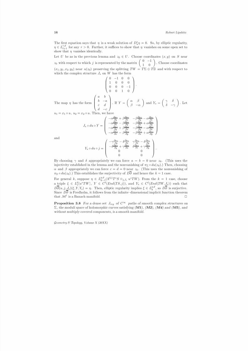
The first equation says that η is a weak solution of D∗uη = 0. So, by elliptic regularity,
η ∈ Lr,dℓ+1 for any r > 0. Further, it suffices to show that η vanishes on some open set to
show that η vanishes identically.
Let U be as in the previous lemma and z0 ∈ U . Choose coordinates (x, y) on S near
z0 with respect to which j is represented by the matrix
0 −11 0
. Choose coordinates
(x1, y1, x2, y2) near u(z0) preserving the splitting T W = T Σ ⊕ T D and with respect towhich the complex structure J s on W has the form
0 −1 0 01 0 0 00 0 0 −10 0 1 0
.
The map η has the form
a bb −ac dd −c
. If Y =
α β β −α
and Y s =
γ δδ −γ
. Let
u1 = x1 u, u2 = x2 u. Then, we have
J s du Y =
−α∂u1
∂y + β ∂u1∂x −β ∂u1∂y − α∂u1∂x
−α∂u1∂x − β ∂u1∂y −β ∂u1∂x + α∂u1
∂y
−α∂u2∂y + β ∂u2∂x −β ∂u2∂y − α∂u2
∂x
−α∂u2∂x − β ∂u2∂y −β ∂u2∂x + α∂u2
∂y
and
Y s du j =
−γ
∂u1∂y − δ
∂u1∂x γ
∂u1∂x − δ
∂u1∂y
−δ ∂u1∂y + γ ∂u1∂x δ ∂u1∂x + γ ∂u1∂y
0 00 0
.
By choosing γ and δ appropriately we can force a = b = 0 near z0 . (This uses theinjectivity established in the lemma and the nonvanishing of πΣ du(z0).) Then, choosingα and β appropriately we can force c = d = 0 near z0 . (This uses the nonvanishing of πD du(z0).) This establishes the surjectivity of D∂ and hence the k = 1 case.
For general k , suppose η ∈ L p,dk−1(Λ0,1T ∗S ⊗ j,J s u∗T W ). From the k = 1 case, choose
a triple ξ ∈ L p1(u∗T W ), Y ∈ C ℓ(End(TS ,j)), and Y s ∈ C ℓ(End(TW,J s)) such that
D∂ (u,j,J s)(ξ , Y , Y s) = η . Then, elliptic regularity implies ξ ∈ L
p,d
k , so D∂ is surjective.Since D∂ is Fredholm, it follows from the infinite–dimensional implicit function theoremthat Mℓ is a Banach manifold. 2
Proposition 3.8 For a dense set J reg of C ∞ paths of smooth complex structures onΣ, the moduli space of holomorphic curves satisfying ( M1), ( M2 ), ( M4) and ( M5 ), andwithout multiply covered components, is a smooth manifold.
Geometry & T opology , Volume X (20XX)
8/3/2019 Robert Lipshitz- A Cylindrical Reformulation of Heegaard Floer Homology
http://slidepdf.com/reader/full/robert-lipshitz-a-cylindrical-reformulation-of-heegaard-floer-homology 17/135
A Cylindrical Reformulation of Heegaard Floer Homology 17
Proof. Observing that (M2) implies the absence of annoying curve components, this
follows easily from the previous result. The set J reg is exactly the set of regular values forthe projection of M onto J . For J ℓ it is immediate from Smale’s infinite–dimensionalversion of Sard’s theorem that J ℓreg is dense. For the C ∞ statement a short approximationargument is required. We refer the reader to [14, page 36]; our case is just the same astheirs. 2
Remark. Note that (M6) implies that u has no multiply covered components.
We will often say a complex structure J achieves transversality to mean J ∈ J reg .
There is a second way that we can sometimes achieve transversality, which is more conve-nient for computations: by keeping the complex structure on W split and perturbing theα and β circles. Specifically
Proposition 3.9 Suppose that a homology class A ∈ π2(x, y) with ind(A) = 1 is suchthat any jΣ × jD–holomorphic curve u : S → W in the homology class A must have πΣ u|∂S somewhere injective. Then for a generic perturbation of the α– and β –circles,for any u in the homology class A the linearization D∂ , computed with respect to the complex structure jΣ × jD on W , is surjective.
The proof of this proposition is analogous to the argument in [16]. It is also a corollaryof [21, Proposition 3.9], so we omit the proof.
We shall refer to the condition in the preceding proposition as boundary injectivity. Oneobvious time when boundary injectivity holds is
Lemma 3.10 Suppose the homology class A ∈ π2(x, y) is represented by a domain D =i niDi such that for some i and j , ni = 1, n j = 0, and ∂Di ∩ ∂D j = ∅. Then A satisfies
the boundary injectivity hypothesis.
For computing the homologies defined in Section 8, if the boundary injectivity criterionis met by every domain with index 1 it will suffice to take a generic perturbation of theboundary conditions and the split complex structure jΣ × jD rather than a generic pathJ s of complex structures. (The only time this is relevant in this paper is Section 11, butin practice it is necessary for most direct computations.)
4 Index
In this section we compute the index of the linearized ∂ –operator D∂ at a holomorphic mapu : (S, j) → (W, J ). We start by reducing to a result discussed in [1] via a doubling argu-ment similar to the one found in [10]. We then reinterpret this index several times, obtaining
Geometry & T opology , Volume X (20XX)
8/3/2019 Robert Lipshitz- A Cylindrical Reformulation of Heegaard Floer Homology
http://slidepdf.com/reader/full/robert-lipshitz-a-cylindrical-reformulation-of-heegaard-floer-homology 18/135
18 Robert Lipshitz
the Chern class formula for the index of periodic domains (Corollary 4.12, which is [21,
Theorem 4.9]), J. Rasmussen’s formula ([25, Theorem 9.1], proved here in Proposition 4.8)and a combinatorial formula for the index near an embedded curve (Corollary 4.3) and,consequently, the Maslov index in traditional Heegaard Floer homology (Corollary 4.10).
4.1 First formulas for the index.
We may assume that J is split, since deformations of J will not change the index. Also,we assume that the α and β curves meet in right angles.
Let a1, . . . , ag be the components of the boundary of S (in the complement of the punc-tures) mapped to α–cylinders and b1, . . . , bg the components mapped to β –cylinders. We
define the quadruple of S , denoted 4⋉S , by gluing four copies of S , denoted S 1 , S 2 , S 3 ,and S 4 , as follows. Glue each ai in S 1 to ai in S 2 and each ai in S 3 to ai in S 4 . Similarly,glue each bi in S 1 to bi in S 3 and each bi in S 2 to bi in S 4 . Define a complex structureon 4⋉ S by taking the complex structure j on S 1 and S 4 and its conjugate j on S 2 andS 3 . Notice that these complex structures glue together correctly.
The complex vector bundle (u∗TW,u∗J ) extends to a vector bundle over 4 ⋉ S , whichwe denote (u∗T W , J ), in an obvious way, and D∂ extends to an operator 4 ⋉D∂ on thesections of this vector bundle. We restrict 4⋉D∂ to the space of sections which approachzero near each puncture, as we require fixed asymptotics.
By [1, Corollary 5.4, p. 53], the index of 4 ⋉D∂ is
−χ(4⋉ S ) + 2c1(A). (4)
Here, c1(A) is defined as follows. Choose a small disk near each point in α∩β . Trivialize(T Σ, J ) over these disks. This gives a trivialization of u∗T W in a neighborhood of thepunctures in 4 ⋉ S which extends to a trivialization of u∗T W over the surface 4⋉ S obtained by filling in the punctures. Then, c1(A) is the pairing of the first Chern classof u∗T W with the fundamental class of 4⋉ S . Note that since T ([0, 1] × R) is trivial, tocompute c1 we need only look at the Σ factor. Also, it is necessary to observe that F.Bourgeois’s calculations in [1, Section 5] are all done in the pullback bundle, so the factthat our index problem does not correspond to a genuine map is a nonissue.
We convert Formula (4) into one not involving the quadruple of S . First we compute that
χ(4⋉
S ) = 4χ(S ) − 4g . Indeed, after doubling along the α–arcs the Euler characteristic is2χ(S ) − g . Doubling again we obtain χ(4⋉ S ) = 2(2χ(S ) − g) − 2g . (The last summandof −2g comes from the 2g punctures in 4⋉ S .)
Second, c1(A) can be computed from Maslov–type indices as follows. Choose the trivializa-tions of T W over the neighborhoods V of α∩β above so that for p ∈ α∩β , T pβ = R ⊂ C
and T pα = iR ⊂ C. Trivialize (πΣ u)∗T Σ over S so that this trivialization agrees with
Geometry & T opology , Volume X (20XX)

8/3/2019 Robert Lipshitz- A Cylindrical Reformulation of Heegaard Floer Homology
http://slidepdf.com/reader/full/robert-lipshitz-a-cylindrical-reformulation-of-heegaard-floer-homology 19/135
A Cylindrical Reformulation of Heegaard Floer Homology 19
Obtuse Corner Acute Corner
Figure 2: S is the shaded region.
the specified trivialization of T W over the neighborhoods V . Then, each boundary arc aior bi gives a loop of lines in C, and so has a well–defined Maslov index µ(ai) or µ(bi). Itis not hard to see that c1(A) = 2(
gi=1 µ(ai) − µ(bi)). This is independent of the choice
of trivialization subject to the specified criteria.
Fix a map u : (S,∂S ) → (W, C α ∪ C β ). An argument almost exactly like the one in [10]shows that
ind(D∂ ) =1
4
ind(4⋉D∂ ) = g − χ(S ) +
g
i=1
µ(ai) −g
i=1
µ(bi). (5)
The factor of 1/4 comes from the “matching conditions” on the boundary of S .
We again reinterpret the Maslov indices. Given a domain D , we define the Euler measureof D as follows. Suppose first that D is a surface with boundary and corners. Choose ametric on D such that ∂D is geodesic and such that the corners of D are right angles.Then the Euler measure e(D) is defined to be 1
2π times the integral over D of the curvatureof the metric. (This is normalized so that the Euler measure of a sphere is 2, agreeing withits Euler characteristic.) From this definition it is clear that the Euler measure is additiveunder disjoint unions and gluing of components along boundaries, and so the definitionextends naturally to domains (linear combinations of regions in Σ).
It follows from the Gauss–Bonnet theorem that the Euler measure of a surface S with kacute right–angled corners (see Figure 2) and ℓ obtuse right–angled corners is χ(S )−k/4+ℓ/4. As with the previous formulation of Euler measure, this formula is additive, so theEuler measure of a domain D =
i Di is e(D) =
i e(Di).
From the Gauss–Bonnet theorem, we also know that if we endow D with a flat metricsuch that all corners are right angles then the Euler measure e(D) is 1
2π times the geodesic
Geometry & T opology , Volume X (20XX)

8/3/2019 Robert Lipshitz- A Cylindrical Reformulation of Heegaard Floer Homology
http://slidepdf.com/reader/full/robert-lipshitz-a-cylindrical-reformulation-of-heegaard-floer-homology 20/135
20 Robert Lipshitz
Figure 3: A degenerate corner
curvature of ∂D . It is then clear that for D the domain corresponding to u,g
i=1 µ(ai) −µ(bi) = 2e(D). So, we can recast the index formula as
ind(D∂ ) = g − χ(S ) + 2e(D). (6)
4.2 Determining S from A.
Note that the formulas for the index derived so far depend not only on the homology classbut also on the topological type of the source. This is as it should be. However, as we willshow presently, for embedded holomorphic curves the Euler characteristic of the source isdetermined by the homology class. (Actually, we prove this more generally for any curvessatisfying certain hypotheses described in Lemma 4.1 below, not just holomorphic ones.)In fact, we can give an explicit formula for the Euler characteristic, allowing us to givea combinatorial formula for the index. We will see in Subsection 4.3 that this formulacalculates the Maslov index in the setup of [21] as well. Before proving this claim weintroduce some more terminology and notation.
Given an intersection point x we call each xi ∈ x a corner of x. Following Rasmussen, wedefine a corner xi of x to be degenerate for a homology class A ∈ π2(x, y) if xi = y j forsome y j ∈ y . This definition will be convenient presently.
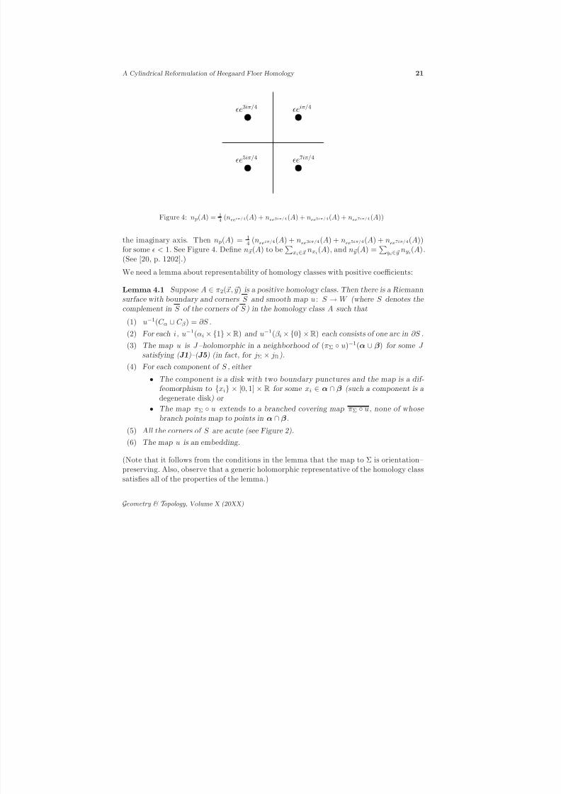
Let p ∈ αi ∩ β j . For a homology class A ∈ π2(x, y), define n p(A) to be the average of thecoefficients of A of the four cells with corners at p. More precisely, choose coordinates iden-tifying a neighborhood of p in Σ with the unit disk in C, αi with the real axis, and β j with
Geometry & T opology , Volume X (20XX)
8/3/2019 Robert Lipshitz- A Cylindrical Reformulation of Heegaard Floer Homology
http://slidepdf.com/reader/full/robert-lipshitz-a-cylindrical-reformulation-of-heegaard-floer-homology 21/135
A Cylindrical Reformulation of Heegaard Floer Homology 21
ǫe3iπ/4
ǫe5iπ/4 ǫe7iπ/4
ǫeiπ/4
Figure 4: n p(A) = 14 (nǫeiπ/4(A) + nǫe3iπ/4(A) + nǫe5iπ/4(A) + nǫe7iπ/4(A))
the imaginary axis. Then n p(A) = 14 (nǫeiπ/4(A) + nǫe3iπ/4(A) + nǫe5iπ/4(A) + nǫe7iπ/4(A))
for some ǫ < 1. See Figure 4. Define nx(A) to be
xi∈xnxi(A), and n y(A) =
yi∈ y
nyi(A).(See [20, p. 1202].)
We need a lemma about representability of homology classes with positive coefficients:
Lemma 4.1 Suppose A ∈ π2(x, y) is a positive homology class. Then there is a Riemannsurface with boundary and corners S and smooth map u : S → W (where S denotes the complement in S of the corners of S ) in the homology class A such that
(1) u−1(C α ∪ C β ) = ∂S .(2) For each i, u−1(αi × 1 ×R) and u−1(β i × 0 ×R) each consists of one arc in ∂S .
(3) The map u is J –holomorphic in a neighborhood of (πΣ u)−1(α ∪ β) for some J satisfying ( J1)–( J5 ) (in fact, for jΣ × jD ).
(4) For each component of S , either
• The component is a disk with two boundary punctures and the map is a dif-feomorphism to xi × [0, 1] × R for some xi ∈ α ∩ β (such a component is a degenerate disk) or
• The map πΣ u extends to a branched covering map πΣ u, none of whose branch points map to points in α ∩ β .
(5) All the corners of S are acute (see Figure 2).(6) The map u is an embedding.
(Note that it follows from the conditions in the lemma that the map to Σ is orientation–preserving. Also, observe that a generic holomorphic representative of the homology classsatisfies all of the properties of the lemma.)
Geometry & T opology , Volume X (20XX)
8/3/2019 Robert Lipshitz- A Cylindrical Reformulation of Heegaard Floer Homology
http://slidepdf.com/reader/full/robert-lipshitz-a-cylindrical-reformulation-of-heegaard-floer-homology 22/135
22 Robert Lipshitz
0 0 0 0 0
0 0 0 0 0
0 0 0 0 0
0 0 0 0 0
0 0 0 0 0
0 0 0 0 0
0 0 0 0 0
0 0 0 0 0
1 1 1 1 1
1 1 1 1 1
1 1 1 1 1
1 1 1 1 1
1 1 1 1 1
1 1 1 1 1
1 1 1 1 1
1 1 1 1 1
0 0 0 0 0 0 0
0 0 0 0 0 0 0
0 0 0 0 0 0 0
0 0 0 0 0 0 0
0 0 0 0 0 0 0
1 1 1 1 1 1 1
1 1 1 1 1 1 1
1 1 1 1 1 1 1
1 1 1 1 1 1 1
1 1 1 1 1 1 1
0 0 0 0 0
0 0 0 0 0
0 0 0 0 0
0 0 0 0 0
1 1 1 1 1
1 1 1 1 1
1 1 1 1 1
1 1 1 1 1
0 0 0 0 0 0 0
0 0 0 0 0 0 0
0 0 0 0 0 0 0
0 0 0 0 0 0 0
1 1 1 1 1 1 1
1 1 1 1 1 1 1
1 1 1 1 1 1 1
1 1 1 1 1 1 1
0 0 0 0
0 0 0 0
0 0 0 0
0 0 0 0
1 1 1 1
1 1 1 1
1 1 1 1
1 1 1 1
Domain
Sα
β
1
2 1
0
S
One possible S
Another possible S
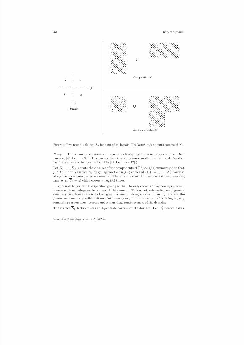
Figure 5: Two possible gluings S 0 for a specified domain. The latter leads to extra corners of S 0 .
Proof. (For a similar construction of a u with slightly different properties, see Ras-mussen, [25, Lemma 9.3]. His construction is slightly more subtle than we need. Anotherinspiring construction can be found in [21, Lemma 2.17].)
Let D1, · · · , DN denote the closures of the components of Σ \ (α∪β), enumerated so that zi ∈ Di . Form a surface S 0 by gluing together nzi(A) copies of Di (i = 1, · · · , N ) pairwisealong common boundaries maximally. There is then an obvious orientation–preservingmap pΣ,0 : S 0 → Σ which covers zi nzi(A) times.
It is possible to perform the specified gluing so that the only corners of S 0 correspond one–to–one with non–degenerate corners of the domain. This is not automatic; see Figure 5.One way to achieve this is to first glue maximally along α–arcs. Then glue along theβ –arcs as much as possible without introducing any obtuse corners. After doing so, anyremaining corners must correspond to non–degenerate corners of the domain.
The surface S 0 lacks corners at degenerate corners of the domain. Let D22 denote a disk
Geometry & T opology , Volume X (20XX)
8/3/2019 Robert Lipshitz- A Cylindrical Reformulation of Heegaard Floer Homology
http://slidepdf.com/reader/full/robert-lipshitz-a-cylindrical-reformulation-of-heegaard-floer-homology 23/135
A Cylindrical Reformulation of Heegaard Floer Homology 23
with two punctures on the boundary. Let S 1 denote the disjoint union of S 0 with a copy
of D22 for each degenerate corner of the domain. Extend pΣ,0 to a map pΣ,1 from D22 bymapping one copy of D2
2 to each degenerate corner of the domain.
Now, S 0 inherits a complex structure from Σ. Extend this complex structure arbitrarilyover the new disks in S 1 to obtain a complex structure on S 1 . It is easy to choose a map pD,1 : S 1 → [0, 1]×R such that the map ( pΣ,1× pD,1) : S 1 → W satisfies all of the propertiesspecified in the statement of the lemma except perhaps numbers (2) and (6). Perturbing pD,1 we may assume that ( pΣ,1 × pD,1) is an embedding except for a collection of transversedouble points.
For each αi (respectively β j ), there will be exactly one arc in ∂ Σ1 mapped by pΣ,1 to αi
(respectively β j ), and possibly some circles in ∂ Σ1 mapped by pΣ,1 to αi (respectively
β j ). The map pD,1 must be constant near each closed component of ∂S 1 , and the imageof the arc under ( pΣ,1 × pD,1) must intersect the image of each closed component of ∂S 1mapped to αi (respectively β j ) exactly once.
Modifying S 1 and pΣ,1 × pD,1 near the double points of pΣ,1 × pD,1 we can obtain a newmap u : S → W satisfying all of the stated properties: in the process of deforming awaythe double points, we necessarily achieve property (2) as well. 2
Proposition 4.2 Let u : S → W be a map satisfying the conditions enumerated in the previous lemma, representing a homology class A. Then the Euler characteristic χ(S ) is given by
χ(S ) = g − nx(A) − n y(A) + e(A). (7)
Proof. Applying the Riemann–Hurwitz formula to πΣ u, we only need to calculate thedegree of branching of πΣ u.
To calculate the number of branch points of πΣ u we reinterpret this number as a self–intersection number. We will assume all branch points of πΣ u have order 2; we canclearly arrange this. Observe that since S has no obtuse corners, by the Riemann–Hurwitzformula,
χ(S ) = e(S ) + g/2 = e(A) − (number of branch p oints) +1
2(number of trivial disks)+ g/2.
(Branch points on ∂S should each be counted as half of a branch point.)
Assume for the time being that u contains no trivial disks, and in fact has no degeneratecorners.
Notice that the number of branch points of πΣ u is equal to the number of times thevector field ∂
∂t is tangent to u. (Tangencies on ∂S should each be counted as half of a
Geometry & T opology , Volume X (20XX)
8/3/2019 Robert Lipshitz- A Cylindrical Reformulation of Heegaard Floer Homology
http://slidepdf.com/reader/full/robert-lipshitz-a-cylindrical-reformulation-of-heegaard-floer-homology 24/135
24 Robert Lipshitz
tangency.) Let u′ denote the curve obtained from u by translating a distance R in the
R–direction. Then, for small R, the number of branch points of πΣ u is equal to theintersection number of u and u′ . (Intersections on ∂S should each be counted as half of an intersection.)
This intersection number is invariant under isotopies of u′ such that all intersection pointsof u and u′ remain in a compact subset of of W . (The only thing to check is thatwhen an intersection point in the interior of W hits the boundary it gives rise to a pairof intersection p oints on the boundary. It is not hard to check this using a doublingargument in a neighborhood of the boundary.) We will calculate the intersection numberby translating u′ far in the R–direction of W .
Translate u′ by some R ≫ 0 in the R–factor of W . All intersection points between u and
u′
stay in a compact subset of W , so the intersection number #u ∩ u′
is unchanged.We can modify u′ so that near each negative puncture (corresponding to some xi ) u′
agrees with the trivial disk xi × [0, 1] × R. Further, we can do this modification so thatall intersection points between u and u′ stay within some compact subset of W . (Thisfollows from the simple asymptotic behavior of u′ near −∞.)
Similarly, we can modify u so that near the positive punctures of S , u agrees with thetrivial disks yi × [0, 1] ×R ensuring in the process that all intersection points between uand u′ stay within some compact subset of W .
Finally, for R large enough, we can assume that after the two modifications every in-tersection point between u and u′ corresponds to an intersection point between u and
xi × [0, 1] ×R or between y j × [0, 1] × R and u′ .
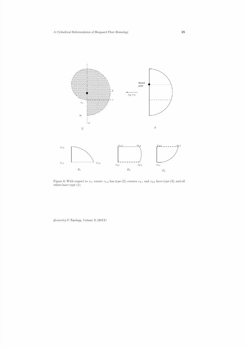
Now, for each corner ck,ℓ of each component E k of S \ (πΣ u)−1(α ∪ β), one of thefollowing four phenomena occurs:
(1) The corner ck,ℓ is mapped by πΣ u somewhere other than xi . That is, lim p→ck,ℓ πΣu( p) = xi .
(2) The corner ck,ℓ is mapped by πΣ u to xi , but at −∞. That is, lim p→ck,ℓ πΣ u( p) =xi but lim p→ck,ℓ πR u( p) = −∞.
(3) The corner ck,ℓ is mapped by πΣ u to xi , and is mapped by u to the boundary of W . That is, πΣ u(ck,ℓ) = xi and πD u(ck,ℓ) ∈ ∂ [0, 1] × R.
(4) The corner ck,ℓ is mapped by πΣ u to xi , and is mapped by u to the interior of W . That is, πΣ u(ck,ℓ) = xi and πD u(ck,ℓ) ∈ (0, 1) × R.
(Compare Figure 6.)
In the first two cases, E k does not contribute to #(u ∩ xi × [0, 1] × R). In the lasttwo, E k contributes 1/4 to the intersection number. Notice that the second case occurs
Geometry & T opology , Volume X (20XX)
8/3/2019 Robert Lipshitz- A Cylindrical Reformulation of Heegaard Floer Homology
http://slidepdf.com/reader/full/robert-lipshitz-a-cylindrical-reformulation-of-heegaard-floer-homology 25/135

8/3/2019 Robert Lipshitz- A Cylindrical Reformulation of Heegaard Floer Homology
http://slidepdf.com/reader/full/robert-lipshitz-a-cylindrical-reformulation-of-heegaard-floer-homology 26/135
26 Robert Lipshitz
exactly once, since S has no obtuse corners. There are a total of 4nx corners satisfy-
ing one of conditions (2)–(4) for some xi . Exactly g of them satisfy condition (2). So,# (u ∩ xi × [0, 1] ×R) = nx − g/4.
A similar analysis works for the intersection points between u′ and y j × [0, 1] × R. So,it follows that the intersection number between u and u′ is
#(u ∩ u′) = nx(A) + n y(A) − g/2.
It follows that
χ(S ) = e(A) − nx(A) − n y(A) + g.
In the proof so far we assumed that there were no trivial disks. Suppose u contains trivial
disks corresponding to the intersection points xi1, · · · , xik . Since we are considering onlyembedded curves, nxij (A) = 0 for j = 1, · · · , k . By the argument above, after ignoring
the trivial disks, we find #(u ∩ u′) = nx(A) + n y(A) − g/2 + k/2. So, we have the sameformula for χ(S ) as before.
Finally, we deal with degenerate corners which are not trivial disks. Since we are assumingS has only acute corners, and acute degenerate corners have exactly one shared boundarycomponent under πΣ u, it is easy to see that after translating in the R–direction, therewill be one intersection point along the boundary near the puncture, so the extra cornermapped to ±∞ contributes 1
2 to the intersection number, as one would expect from ourformula. This concludes the proof. 2
Note that if u : S → W is an embedded holomorphic curve (with respect to any complexstructure J on W satisfying (J1)–(J5)) then, after slitting S near any obtuse corners andperturbing u slightly, u : S → W satisfies the conditions of Lemma 4.1. It follows thatProposition 4.2 calculates the Euler characteristic of S .
Corollary 4.3 For A a positive homology class and u : S → W a representative for Asatisfying the conditions of Lemma 4.1, the index of the D∂ operator near u is given by
ind(D∂ ) = e(A) + nx(A) + n y(A) (8)
Proof. This is immediate from formula (6) and Proposition 4.2. 2
Definition 4.4 Given a positive homology class A define the index ind(A) of A to be the index of the D∂ operator near any curve satisfying the conditions of Lemma 4.1.
Corollary 4.5 If A and A + k[Σ] are both positive then ind(A + k[Σ]) = ind(A) + 2k .
Geometry & T opology , Volume X (20XX)
8/3/2019 Robert Lipshitz- A Cylindrical Reformulation of Heegaard Floer Homology
http://slidepdf.com/reader/full/robert-lipshitz-a-cylindrical-reformulation-of-heegaard-floer-homology 27/135
A Cylindrical Reformulation of Heegaard Floer Homology 27
Proof. By Corollary 4.3,
ind(A + k[Σ]) = e(A + k[Σ]) + nx(A + k[Σ]) + n y(A + k[Σ])
= e(A) + (2 − 2g)k + nx(A) + gk + n y(A) + gk
= e(A) + n x(A) + n y(A) + 2k
= ind(A) + 2k.
2
Definition 4.6 For any homology class A define the index ind(A) of A to be ind(A +k[Σ]) − 2k where k is chosen large enough that A + k[Σ] is positive.
Corollary 4.7 Suppose that A ∈ π2(x, y) and A′ ∈ π2(y, z). Then ind(A + A′) =
ind(A) + ind(A′
).
Proof. We may clearly assume that A and A′ are both positive. Let u : S → W andu′ : S ′ → W be maps satisfying the conditions Lemma 4.1 representing A and A′ respec-tively. Then we can glue u and u′ to a map uu′ : SS ′ → W representing A+A′ . It followsfrom general gluing results for the index that ind(D∂ )(uu′) = ind(D∂ )(u) + ind(D∂ )(u′).(Alternately, it follows from the additivity of Formula (6) under gluing.) 2
Remark. Formula (8) was suggested to me by Z. Szabo. Specifically, he suggested that itseemed the Maslov index in [21] can be calculated by this formula. In particular, in thespecial case when A ∈ π2( x, x), Ozsvath and Szabo proved ([21, Theorem 4.9] and [20,Proposition 7.5]) that Formula (8) does computes the Maslov index. Note that it is not
even clear a priori that Formula (8) is additive. In fact, I do not know a more direct proof than the one we used to obtain Corollary 4.7.
4.3 Comparison with classical Heegaard Floer homology.
In this subsection we assume familiarity with [21].
By considering domains, for example, there is a natural identification of our π2(x, y) withπ2(x, y) as defined in [21, Section 2.4]. For A ∈ π2(x, y), let µ(A) denote the Maslov indexof A, viewed as a homotopy class of maps disks in (Symg(Σ), T α ∪ T β ). The goal of thissubsection is to prove the following
Proposition 4.8 For A ∈ π2(x, y) we have ind(A) = µ(A).
Proof. It is possible to give a direct proof (see [25, proof of Theorem 9.1]), but instead of doing so we will show our formula agrees with the one given by Rasmussen in [25, Theorem9.1]. He proves that at a disk φ : (D, ∂ D) → (Symg(Σ), T α ∪ T β ),
µ(φ) = ∆ · φ + 2e(φ). (9)
Geometry & T opology , Volume X (20XX)
8/3/2019 Robert Lipshitz- A Cylindrical Reformulation of Heegaard Floer Homology
http://slidepdf.com/reader/full/robert-lipshitz-a-cylindrical-reformulation-of-heegaard-floer-homology 28/135
28 Robert Lipshitz
Here, e is the Euler measure defined in Subsection 4.1 and ∆ ·φ is the algebraic intersection
number of φ with the diagonal in Symg(Σ). (The diagonal is an algebraic subvariety of Symg(Σ) of real codimension 2 so the intersection number is well–defined.)
To compare his result with ours, we need a slight strengthening of Lemma 4.1:
Lemma 4.9 Suppose A is a positive homology class. Then we can represent A + [Σ] by a map u : S → W satisfying all the conditions of Lemma 4.1 and such that, additionally,
• The map πD u is a g –fold branched covering map with all its branch points of order 2
• The map u is holomorphic near the preimages of the branch points of πD u.
Proof. Construct a map u1 : S 1 → W representing A as in Lemma 4.1. We would like
to say that we can then choose a branched cover pD,1 : S 1 → [0, 1] × R (mapping arcs onthe boundary appropriately). This may not, however, b e the case: suppose, for instance,that g = 2 and S 1 were the disjoint union of a disk and a surface of genus one with oneboundary component.
However, note that [Σ] ∈ π2(y, y) can be represented by a map with connected source.Specifically, let S Σ be obtained by making small slits in Σ along αi and β i starting atyi ∈ y for i = 1, · · · , g . There is an obvious map S Σ → Σ.
Gluing the negative corners of S Σ to the positive corners of S 1 we obtain a connectedsurface S 2 and map pΣ,2 : S 2 → Σ. Since S 2 is connected it is possible to choose abranched covering map pD,2 : S 2 → D with appropriate boundary behavior. Perturbingthis map we can assume all of its branch points have order 2. Finally, deforming away thedouble points of pΣ,2 × pD,2 and perturbing it to be holomorphic in appropriate places, weobtain an embedding satisfying the specified conditions. 2
Now, fix a positive homology class A in π2(x, y) and a map u representing A as in theprevious lemma. The map u induces a map φ : D → Symg(Σ) as follows. For a ∈ D let(πD u)−1(a) = a1, . . . , ag. Then define φ(a) = πΣ u(a1), . . . , πΣ u(ag).
There is a one–to–one correspondence between order 2 branch points of πD u andtransverse intersections of φ with the top–dimensional stratum of the diagonal. By theRiemann–Hurwitz formula, χ(S ) = gχ(D2) − φ · ∆ = g − φ · ∆, so ind(D∂ )(u) = g − χ(S ) +2e(A + [Σ]) = φ · ∆ + 2e(A + [Σ]).
This is exactly Rasmussen’s formula for the Maslov index. Thus, we have shown that
ind(A + [Σ]) = µ(A + [Σ]) for A positive. But both ind and µ are additive, and haveind([Σ]) = µ([Σ]) = 2. Thus, it follows that ind(A) = µ(A) for all A. 2
Corollary 4.10 In Heegaard Floer homology, the Maslov index of a domain D is givenby
µ(D) = nx(D) + n y(D) + e(D).
Geometry & T opology , Volume X (20XX)
8/3/2019 Robert Lipshitz- A Cylindrical Reformulation of Heegaard Floer Homology
http://slidepdf.com/reader/full/robert-lipshitz-a-cylindrical-reformulation-of-heegaard-floer-homology 29/135
A Cylindrical Reformulation of Heegaard Floer Homology 29
Remark. There are no assumptions on the domain.
4.4 Index for A ∈ π2(x, x).
The following result, which we will use below, is proved by Ozsv ath and Szabo in [20,Proposition 7.5] by direct geometrical argument.
Lemma 4.11 If x ∈ s and A ∈ π2(x, x) then c1( s), A = e(A) + 2nx(A). Here ·, ·denotes the natural pairing between homology and cohomology, c1( s) the first Chern class of s, and A is viewed as an element of H 2(Y ).
The following is completely analogous to [21, Theorem 4.9].
Corollary 4.12 Let P be a homology class in π2(x, x). Then
ind(P ) = c1( s), P + 2nz(P ).
5 Admissibility Criteria
In order to define the differential in our chain complexes it will be important that forany intersection points x and y , only finitely many homology classes A ∈ π2(x, y) withind(A) = 1 support holomorphic curves. For a rational homology sphere, this is automatic:there are only finitely many homology classes in π
2(x, y). In general, following [21], we use
special Heegaard diagrams and “positivity of domains” to ensure that only finitely manyhomology classes support holomorphic curves. Our definitions are the same as theirs. Forthe reader’s amusement, we provide slightly different proofs of two of the fundamentallemmas about admissibility.
Definition 5.1 The pointed Heegaard diagram (Σ, α, β, z) is called weakly admissible for the SpinC–structure s if every nontrivial periodic domain P with c1( s), P = 0 has both positive and negative coefficients. (Compare [21, Definition 4.10].)
Definition 5.2 The pointed Heegaard diagram (Σ, α, β, z) is called strongly admissiblefor the SpinC–structure s if every nontrivial periodic domain P with c1( s), P = 2n > 0
has nzi(P ) > n for some zi . (Compare [21, Definition 4.10].)
Remark. Notice that for any SpinC–structure, c1( s) is an even cohomology class: c1( s)is the first Chern class of v⊥ for some nonvanishing vector field v . Then c1( s) ≡ w2(v⊥)mod 2. Since T M is trivial and the line field determined by v is obviously trivial, 1 =(1 + w1(v⊥) + w2(v⊥)), so w2(v⊥) = 0.
Geometry & T opology , Volume X (20XX)
8/3/2019 Robert Lipshitz- A Cylindrical Reformulation of Heegaard Floer Homology
http://slidepdf.com/reader/full/robert-lipshitz-a-cylindrical-reformulation-of-heegaard-floer-homology 30/135
30 Robert Lipshitz
We now need two kinds of result. The first is the finiteness mentioned just above in the
case of weak / strong admissibility. The second is that the admissibility criteria can beachieved, and that any two admissible Heegaard diagrams can be connected by a sequenceof Heegaard moves through admissible diagrams.
First, a few simple observations. A SpinC–structure is called “torsion” if c1( s) is a torsionhomology class. For a torsion SpinC–structure, c1( s), P = 0 for any periodic class P .So, the two definitions of admissibility agree. Further, if a Heegaard diagram is weakly(or equivalently strongly) admissible for some torsion SpinC–structure then it is weaklyadmissible for every SpinC–structure. This point is useful for computations.
Both admissibility criteria are, obviously, vacuous for a rational homology sphere.
It will be useful to have equivalent definitions of weak / strong admissibility:
Lemma 5.3 Fix a pointed Heegaard diagram H = (Σ, α, β, z) and a SpinC–structure s.
• The diagram H is weakly admissible for s if and only if there is an area form on Σwith respect to which every periodic domain P with c1( s), P = 0 has zero signedarea. (Compare [21, Lemma 4.12].)
• The diagram H is strongly admissible for s if there is an area form on Σ with respectto which every periodic domain P with c1( s), P = 2n has signed area equal to n,and with respect to which Σ has area 1.
Proof. The proofs of the two statements are very similar, and the proof of the first
statement is in [21, Lemma 4.12]. We give here only the proof of the second statement.Let Di, i = 1, · · · , N denote the components of Σ \ (α ∪ β). We can view the spaceof periodic domains as a linear subspace V of ZN ⊂ R
N . Suppose an area form assignsthe area ai to Di . Then the area assigned to P is P · (ai), the dot product of the vectorP ∈ RN and the vector (ai). Since this is the only way the area form enters the discussion,we will refer to the vector (ai) as the area form.
Suppose there is an area form (ai) on Σ with respect to which every periodic domainP with c1( s), P = 2n > 0 has signed area equal to n and Σ has area 1. Supposec1( s), P = 2n. Then by assumption P · (ai) = n. So, (P − n[Σ]) · (ai) = 0. Hence,P − n[Σ] must have some positive coefficient. Hence, P must have some coefficient greaterthan n.
The converse is slightly more involved. Note that since area(−P ) = −area(P ), it suffices toconstruct an area form with the desired property for periodic domains with c1( s), P ≥ 0.
By Lemma 4.11, the function which assigns to a periodic domain P the number c1( s), P extends to an R–linear functional ℓ on V . The map v → v − (ℓ(v)/2) [Σ] gives a linearprojection map p : V → ker(ℓ). Let V ′ = p(V ).
Geometry & T opology , Volume X (20XX)

8/3/2019 Robert Lipshitz- A Cylindrical Reformulation of Heegaard Floer Homology
http://slidepdf.com/reader/full/robert-lipshitz-a-cylindrical-reformulation-of-heegaard-floer-homology 31/135
A Cylindrical Reformulation of Heegaard Floer Homology 31
Now, we want to choose a = (ai) orthogonal to V ′ so that ai > 0 for all i. We will show
that one can choose such an a presently; for now, assume that such an a has been chosen.Multiplying a by some positive real number, we can assume that a · [Σ] = 1. Now, forv ∈ V ,
a · v = a · p(v) + (ℓ(v)/2) a · [Σ] = ℓ(v)/2 = c1( s), P /2
as desired.
Finally, we need to show such an a exists. The linear space V is spanned by the periodicdomains P with c1( s), P ≥ 0, so V ′ is spanned by their images under p. Every periodicdomain P with c1( s), P = 2n ≥ 0 has a coefficient bigger than n = ℓ(P )/2, so every p(P ) has a positive coefficient. It is also true that every p(P ) has a negative coefficient: if ℓ(P ) = 0 this follows by applying the hypothesis to −P ; if ℓ(P ) > 0 this follows from the
fact that nz(P ) = 0.Now, we are reduced to showing the following: let V ′ be a subspace of RN such that everynonzero vector in V ′ has both positive and negative coefficients. Then there is a vectororthogonal to V ′ with all its entries positive. The proof of this claim is a linear algebraexercise; see [21, Lemma 4.12]. 2
Now we get to the two lemmas justifying the introduction of our admissibility criteria. Thefollowing is [21, Lemma 4.13].
Lemma 5.4 If (Σ, α, β, z) is weakly admissible for s then for each x, y ∈ s and j, k ∈ Z
there are only finitely many positive homology classes A ∈ π2(x, y) with ind(A) = j andnz(A) = k .
Proof. If A, B ∈ π2(x, y) and ind(A) = ind(B) = j , nz(A) = nz(B) = k then P = A − Bis a periodic domain with c1( s), P = 0. So, we must show that there are only finitelymany periodic domains P with c1( s), P = 0 such that A + P is positive.
Choose an area form on Σ so that the signed area of any periodic domain P withc1( s), P = 0 is zero. The condition that A + P be positive obviously gives a lowerbound for every coefficient of P . This and the condition that the signed area of P is zerogives an upper bound for every coefficient of P . The coefficients are all integers, so theresult is immediate. 2
The following is [21, Lemma 4.14].
Lemma 5.5 If (Σ, α, β, z) is strongly admissible for s then for each x, y ∈ s and j ∈ Z
there are only finitely many positive homology classes A ∈ π2(x, y) with ind(A) = j .
Proof. Fix a homology class A ∈ π2(x, y) with nz(A) = 0 and ind(A) = j0 . Then anyother homology class B ∈ π2(x, y) can be written as A + P + k[Σ] for some integer k and
Geometry & T opology , Volume X (20XX)
8/3/2019 Robert Lipshitz- A Cylindrical Reformulation of Heegaard Floer Homology
http://slidepdf.com/reader/full/robert-lipshitz-a-cylindrical-reformulation-of-heegaard-floer-homology 32/135
32 Robert Lipshitz
periodic domain P . We have ind(B) = j0 + k + c1( s), P . If we assume that ind(B) = j
then c1( s), P = j − j0 − 2k .
Fix an area form such that the area of Σ is 1 and the area of any periodic domain P is12 c1( s), P . Then, the area of P is j− j0
2 − k .
If we impose the condition that B be positive then we automatically get lower bounds forevery coefficient of P (which are independent of k ). Note that k ≥ 0, since k = nzi(B) forsome i. The condition that the area of P be j− j0
2 − k ≤ j− j02 and the lower bound for the
coefficients of P gives an upper bound for the coefficients of P , independent of k . Thiscompletes the proof. 2
The following is [21, Lemma 5.8 and Proposition 7.2]. We refer the reader there for its(somewhat involved but essentially elementary) proof.
Proposition 5.6 Fix a 3–manifold Y and SpinC–structure s on Y .
(1) There is a weakly (respectively strongly) admissible Heegaard diagram for s.
(2) Suppose that H1 = (Σ, α, β, z) and H2 = (Σ′, α′, β ′, z′) are weakly (respectively strongly) admissible Heegaard diagrams for s. Then there is a sequence of pointedHeegaard moves (i.e., Heegaard moves supported in the complement of z) connecting H1 to H2 such that each intermediate Heegaard diagram is weakly (respectively strongly) admissible for s.
6 Orientations
In order to be able to work with Z coefficients, we need to be able to choose orientationsfor the moduli spaces MA in a coherent way. First we need to know that each MA (orequivalently, each MA ) is orientable. Then we will discuss what we mean by a coherentorientation and why such orientations exist. This is all somewhat technical, and we willsometimes supply references rather than details.
Suppose that we have chosen an almost complex structure J that achieves transversality forthe moduli space MA . Then for u ∈ MA the tangent space T uMA is naturally identifiedwith the kernel ker(Du∂ ) of the linearized ∂ operator at u. In fact, the spaces ker(Du∂ )
fit together to form a vector bundle over MA
naturally isomorphic to T MA
. So, orientingMA is the same as trivializing the top exterior power of the vector bundle ker( D∂ ) overMA .
Rather than working with ker(D∂ ) it is better to work with the line bundle L = det(D∂ )which is defined to be the tensor product of the top exterior power of ker( D∂ ) with thedual of the top exterior power of coker(D∂ ). (This is the “determinant line bundle of the
Geometry & T opology , Volume X (20XX)
8/3/2019 Robert Lipshitz- A Cylindrical Reformulation of Heegaard Floer Homology
http://slidepdf.com/reader/full/robert-lipshitz-a-cylindrical-reformulation-of-heegaard-floer-homology 33/135
A Cylindrical Reformulation of Heegaard Floer Homology 33
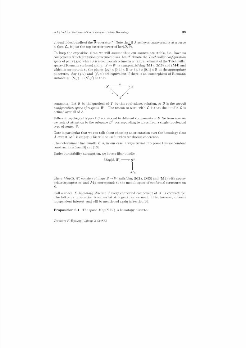
virtual index bundle of the ∂ –operator.”) Note that if J achieves transversality at a curve
u then Lu is just the top exterior power of ker(Du∂ ).
To keep the exposition clean we will assume that our sources are stable, i.e., have nocomponents which are twice–punctured disks. Let T denote the Teichm¨ uller configuration space of pairs ( j,u) where j is a complex structure on S (i.e., an element of the Teichmullerspace of Riemann surfaces) and u : S → W is a map satisfying (M1), (M3) and (M4) andwhich is asymptotic to the planes xi × [0, 1] ×R or yi × [0, 1] ×R at the appropriatepunctures. Say ( j,u) and ( j′, u′) are equivalent if there is an isomorphism of Riemannsurfaces φ : (S, j) → (S ′, j′) so that
S ′
u A A A A
A A A A
φ / / S
u ~ ~ ~ ~ ~ ~ ~ ~ ~ ~
W
commutes. Let B be the quotient of T by this equivalence relation, so B is the moduli configuration space of maps to W . The reason to work with L is that the bundle L isdefined over all of B .
Different topological types of S correspond to different components of B . So from now onwe restrict attention to the subspace BS corresponding to maps from a single topologicaltype of source S .
Note in particular that we can talk about choosing an orientation over the homology classA even if MA is empty. This will be useful when we discuss coherence.
The determinant line bundle L is, in our case, always trivial. To prove this we combineconstructions from [5] and [13].
Under our stability assumption, we have a fiber bundle
Map(S, W ) / / BS
MS
where M ap(S, W ) consists of maps S → W satisfying (M1), (M3) and (M4) with appro-priate asymptotics, and MS corresponds to the moduli space of conformal structures on
S .Call a space X homotopy discrete if every connected component of X is contractible.The following proposition is somewhat stronger than we need. It is, however, of someindependent interest, and will be mentioned again in Section 14.
Proposition 6.1 The space Map(S, W ) is homotopy discrete.
Geometry & T opology , Volume X (20XX)
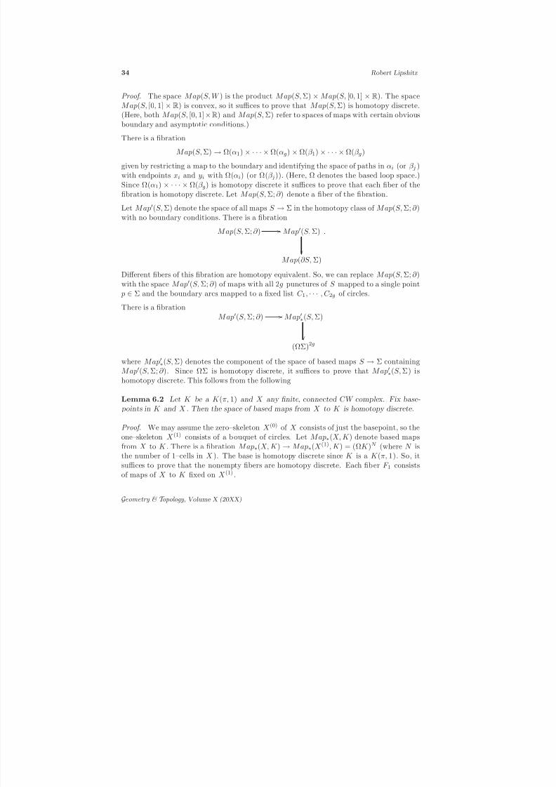
8/3/2019 Robert Lipshitz- A Cylindrical Reformulation of Heegaard Floer Homology
http://slidepdf.com/reader/full/robert-lipshitz-a-cylindrical-reformulation-of-heegaard-floer-homology 34/135
34 Robert Lipshitz
Proof. The space Map(S, W ) is the product M ap(S, Σ) × Map(S, [0, 1] ×R). The space
M ap(S, [0, 1] × R) is convex, so it suffices to prove that Map(S, Σ) is homotopy discrete.(Here, both M ap(S, [0, 1] ×R) and M ap(S, Σ) refer to spaces of maps with certain obviousboundary and asymptotic conditions.)
There is a fibration
M ap(S, Σ) → Ω(α1) × · · · × Ω(αg) × Ω(β 1) × · · · × Ω(β g)
given by restricting a map to the boundary and identifying the space of paths in αi (or β j )with endpoints xi and yi with Ω(αi) (or Ω(β j)). (Here, Ω denotes the based loop space.)Since Ω(α1) × · · · × Ω(β g) is homotopy discrete it suffices to prove that each fiber of thefibration is homotopy discrete. Let M ap(S, Σ; ∂ ) denote a fiber of the fibration.
Let M ap′(S, Σ) denote the space of all maps S → Σ in the homotopy class of M ap(S, Σ; ∂ )with no boundary conditions. There is a fibration
M ap(S, Σ; ∂ ) / / M ap′(S, Σ)
M ap(∂S, Σ)
.
Different fibers of this fibration are homotopy equivalent. So, we can replace M ap(S, Σ; ∂ )with the space M ap′(S, Σ; ∂ ) of maps with all 2g punctures of S mapped to a single point p ∈ Σ and the boundary arcs mapped to a fixed list C 1, · · · , C 2g of circles.
There is a fibration
M ap′
(S, Σ; ∂ ) / / Map′∗(S, Σ)
(ΩΣ)2g
where Map′∗(S, Σ) denotes the component of the space of based maps S → Σ containingM ap′(S, Σ; ∂ ). Since ΩΣ is homotopy discrete, it suffices to prove that M ap′∗(S, Σ) ishomotopy discrete. This follows from the following
Lemma 6.2 Let K be a K (π, 1) and X any finite, connected CW complex. Fix base- points in K and X . Then the space of based maps from X to K is homotopy discrete.
Proof. We may assume the zero–skeleton X (0) of X consists of just the basepoint, so theone–skeleton X (1) consists of a b ouquet of circles. Let Map∗(X, K ) denote based mapsfrom X to K . There is a fibration M ap∗(X, K ) → M ap∗(X (1), K ) = (ΩK )N (where N isthe number of 1–cells in X ). The base is homotopy discrete since K is a K (π, 1). So, itsuffices to prove that the nonempty fibers are homotopy discrete. Each fiber F 1 consistsof maps of X to K fixed on X (1) .
Geometry & T opology , Volume X (20XX)
8/3/2019 Robert Lipshitz- A Cylindrical Reformulation of Heegaard Floer Homology
http://slidepdf.com/reader/full/robert-lipshitz-a-cylindrical-reformulation-of-heegaard-floer-homology 35/135
A Cylindrical Reformulation of Heegaard Floer Homology 35
The proof now proceeds by induction over the skeleta of X . There is a fibration
F 1 → 2–cells
M ap∗(D2, K ; ∂ )
where M ap∗(D2, K ; ∂ ) denotes (based) maps of a disk with the boundary mapped asspecified by the map of the one–skeleton. The base is homotopy discrete, as one deducesfrom the fibration
Map∗(D2, K ; ∂ ) / / Map∗(D2, K )
Ω(K )
in which the total space is contractible and the base space is homotopy discrete. Thus, it
suffices to show that any fiber F 2 of F 1 → 2–cells M ap∗(D2, K ; ∂ ) is contractible. Noticethat each F 2 consists of maps of X specified on the two–skeleton.
Proceeding as before, we have a fibration F 3 →
3–cells M ap∗(D3, K ; ∂ ), now with con-tractible base. It suffices to prove the fiber F 4 is contractible, and so on. Since X is finite,the process terminates at F n for n = dim(X ). 2
Since Σ is a K (π, 1), this completes the proof of the proposition. 2
If the space MS is contractible, or even just has trivial H 1 , then we are finished: we thenhave H 1(BS ) trivial and hence all line bundles over BS are orientable. This is, in fact, thecase if S is a union of disks with boundary punctures. In general, however, MS can haveinteresting topology.
Remark. It is not hard to show, by an argument similar to but simpler than the proof of Proposition 6.1, that the configuration spaces of disks in the original construction of Heegaard Floer homology ([21]) have trivial π1 , proving orientability of the moduli spacesin that setting.
Proposition 6.3 The determinant line bundle L over BS is trivial.
Proof. By Proposition 6.1 for a given source S and homology class A, the space of p ossiblemaps of ∂S is contractible. Then, it follows from the argument of [13, Lemma 6.37] or [5,Lemma 3.8], which we sketch briefly, that the line bundle L is trivial. Fix a map u0 of acollar neighborhood C of ∂S . (By a collar neighborhood, we mean that ∂C is the union
of ∂S and a collection of circles, and each component of C is an annulus with punctureson one of its boundary circles.) We restrict to maps u : S → W agreeing with u0 on C .(That it suffices to consider such maps is the only place we use anything special about oursituation. If we choose u0 to be an embedding, say, it makes sense to say u agrees withu0 on a collar neighborhood of the boundary, even though BS is a fiber bundle and not aproduct of MS and Map(S, W ).)
Geometry & T opology , Volume X (20XX)
8/3/2019 Robert Lipshitz- A Cylindrical Reformulation of Heegaard Floer Homology
http://slidepdf.com/reader/full/robert-lipshitz-a-cylindrical-reformulation-of-heegaard-floer-homology 36/135
36 Robert Lipshitz
Let ∂ in(C ) denote the “interior boundary” of C , i.e., the circles without punctures.
As in Section 3, we are interested in the kernel and cokernel of
D∂ : L p,d1 (u∗TW,∂ ) ⊕ R
2g → L p,d
Λ0,1u∗T W
.
Let S ′ denote the surface obtained from S by collapsing ∂ inC . The operator D∂ inducesan operator D′∂ between bundles over S ′ , and it is not hard to see that the determinantlines of D∂ and D′∂ are naturally identified. Let C ′ be the image of C in S ′ , so S ′
consists of C ′ and some closed components. The determinant line of D′∂ is the tensorproduct of the determinant lines of the restriction of D′∂ to each component of S ′ .
Over the closed components of S ′ the determinant line has a natural “complex” orientation.Fix once and for all trivializations of the determinant lines of D′∂ over the componentsof C ′ . (Since u|
C = u
0, the restriction of D′∂ to C ′ does not depend on u.) Then,
these trivializations induce an orientation of the determinant of D′∂ , and hence of D∂ ,independent of u. This proves orientability of L. 2
Remark. For comparison, in [21], Ozsvath and Szabo only use the fact that the tangentbundles to the Lagrangian submanifolds in question are trivial. In [5], although theirsetup is not quite the same as standard symplectic field theory, T. Ekholm, J. Etnyre andM. Sullivan prove orientability under the assumption that the Lagrangian manifolds inquestion are Spin.
The coherence we want for our orientation system is the following. Suppose that we havemaps u : S → W and u′ : S ′ → W in homology classes A ∈ π2(x, x′) and A′ ∈ π2(x′, x′′),respectively. Then by gluing the positive corners of u to the negative corners of u′ (in some
fixed, concrete way) one can construct a 1–parameter family of curves uru′ : SrS ′ → W .One obtains, thus, an inclusion M apA(T, W ) × M ap′A(T, W ) × (R, ∞) → MapA+A′(T, W ).This inclusion is covered by a map of determinant line bundles. Coherence means that thismap is orientation–preserving. A few more details can be found in the proof of Proposi-tion 13.7, and a complete discussion in any of [6, Section 1.8], [3] or [5].
There are strong general results about the existence of coherent orientations (see [6], [3]or [5]). In our case, however, we can construct them quite concretely:
As in [21, Section 3.6], given a Heegaard diagram, a SpinC–structure s, and an intersectionpoint x0 ∈ s, a complete set of paths for s is a choice of homology class T i ∈ π2(x0, xi)for every other xi ∈ s. Fix x0 ∈ s, a representative P j of each homology class in some
basis for π2(x0, x0) = H 2(Y ), and a complete set of paths for s. By the gluing propertiesof coherent orientations described two paragraphs earlier, specifying a particular coherentorientation of the moduli space is equivalent to specifying an orientation over each T i , eachP j , and over [Σ] ∈ π2(x0, x0).
Over [Σ] there is a canonical orientation, given by viewing the map Σ
∐gk=1D
2
→ Σ×Dgiven by id×0 on Σ and x0,i×id on the ith D2 as positively oriented. We shall always
Geometry & T opology , Volume X (20XX)
8/3/2019 Robert Lipshitz- A Cylindrical Reformulation of Heegaard Floer Homology
http://slidepdf.com/reader/full/robert-lipshitz-a-cylindrical-reformulation-of-heegaard-floer-homology 37/135
8/3/2019 Robert Lipshitz- A Cylindrical Reformulation of Heegaard Floer Homology
http://slidepdf.com/reader/full/robert-lipshitz-a-cylindrical-reformulation-of-heegaard-floer-homology 38/135
38 Robert Lipshitz
Given transversality, Deligne–Mumford type degenerations in the interior of S are pro-
hibited for a generic choice of J because they have codimension 2 in the space of allholomorphic curves. That is, these degenerations have codimension 2 after quotienting bytranslation. Hence, they only occur if ind(A) ≥ 3. This rules out all but one kind of degeneration along the interior: bubbling of a copy of Σ × (s0, t0). (Recall that our com-plex structure does not achieve transversality for maps u with πD u constant.) However,Corollary 4.3 shows that if a copy of Σ were to bubble off then the remainder of v wouldhave to be a collection of trivial disks, and so nzi(A) = 1 for every i. Bubbling more thanone copy of Σ or a multiply covered copy of Σ is prohibited by Corollary 4.3.
So, we need to check that cusp degenerations (i.e., degenerations along arcs with boundaryon ∂S ) are impossible.
Suppose that a cusp degeneration occurs. Let A denote an arc in S which collapses. Sincedifferent components of ∂S are mapped by u to different cylinders in W , both endpoints of A must lie on the same boundary component C of S . Without loss of generality, supposethat C is mapped by the ui to α1 × 1 × R. Let S ′ denote the nodal surface obtainedfrom S by collapsing the arcs along which the complex structure degenerates. In the limitcurve v there will be more than one boundary component mapped to α1 × 1 × R. LetC ′ denote all the boundary components mapped to α1 × 1 × R. Consider the mapπD v|C ′ : C ′ → iR. One of the boundary components in C ′ will have a local (in fact,global) maximum. But this and the open mapping theorem imply that the map πDv mustbe constant near that boundary component, hence constant on a connected component of S ′ . In particular, this implies that all of the boundary of S ′ is mapped to the α–circles.
However, the α–circles are non–separating, so the component of S ′ on which πD v isconstant must be mapped diffeomorphically onto Σ. As above, it then follows from ourindex computation that the rest of v must consist of g trivial disks, and A = [Σ].
Thus, we have proved the each ui satisfies (M0). Condition (M1) is automatically satisfied.
The only way that πD v could be constant on some component of S would be as a resultof bubbling, which we showed is prohibited. This implies (M2) for the limit curves.
Condition (M4) and the condition that there are exactly 2g punctures on each storyalso follow from the maximum modulus, or open mapping, theorem: applying the openmapping theorem to πD u j , one sees that the restriction of πR u j to any componentof ∂S \ p1, · · · , pg , q1, · · · , qg must be monotone, so no new Reeb chords could form as j → ∞.
Since projection onto [0, 1] × R is holomorphic, the open mapping theorem prohibitsany new boundary components from forming. The maximum modulus theorem prohibitsboundary components from disappearing, so (M3) is satisfied by the limit curves.
That condition (M5) is satisfied by the limit curves is part of the statement of the com-pactness theorem [2, Theorem 10.1].
Geometry & T opology , Volume X (20XX)
8/3/2019 Robert Lipshitz- A Cylindrical Reformulation of Heegaard Floer Homology
http://slidepdf.com/reader/full/robert-lipshitz-a-cylindrical-reformulation-of-heegaard-floer-homology 39/135
A Cylindrical Reformulation of Heegaard Floer Homology 39
Let S j denote the source of v j . Suppose that v has height ℓ. Then since all degenerations
in S correspond to level splitting, χ(S ) = (1−ℓ)g+ℓ j=1 χ(S j). Let D j be the domain in Σcorresponding to v j . Then we have e(D) =
ℓ j=1 e(D j). So, ind(ui) = g − χ(S ) + 2e(D) =
ℓg −ℓ
j=1 (χ(S j) + 2e(D j)) =ℓ
j=1 ind(v j). That is, the index formula adds over levels.
Finally, near any immersed curve with the equivalent of k double points and with respectto which the complex structure achieves transversality there is a 2k–dimensional family of embedded holomorphic curves. This shows that the v j must all be embedded. 2
For an almost complex structure J which achieves transversality, it follows from the pre-vious proposition, Proposition A.1 and the compactness Theorem 10.1 from [2] that:
Corollary 7.2 The space of holomorphic curves satisfying ( M0 )–( M6 ) in a given homol-ogy class A (modulo translation in the R–factor of W ) with ind(A) ≤ 2 and A = [Σ]
forms a smooth manifold MA of dimension ind(A) − 1 which is the interior of a com-
pact manifold with boundary MA . The boundary of that manifold ∂ MA consists of all multi–story holomorphic buildings each component of which satisfies ( M0 )–( M6 ) in the homology class A.
8 Chain Complexes
Here we define the four basic chain complexes used by Ozsvath–Szabo – CF , CF ∞
,CF − and CF + . Once these are defined CF ±red are defined in exactly the same way asin [21]. Generalizing our definitions to include the twisted theories of [20, Section 8] isstraightforward.
Fix: a pointed Heegaard diagram (Σ, α, β, z), an almost complex structure J satisfying(J1)–(J5) and achieving transversality, and a coherent orientation system. We shall assumethat the Heegaard diagram satisfies the weak or strong admissibility criterion as necessary.
Fix a SpinC–structure s.
First we define the chain complex
CF . Suppose that our Heegaard diagram is weakly
admissible for s. Recall that, by Lemma 5.4, for x, y ∈ s, there are only finitely manyA ∈ π2(x, y) and nzi(A) ≥ 0 for all i and ind(A) = 1. Let CF (Y, s) be the free Abeliangroup generated by the intersection points x.
Define M(x, y) =
A∈π2( x, y), ind(A)=1
MA
Geometry & T opology , Volume X (20XX)
8/3/2019 Robert Lipshitz- A Cylindrical Reformulation of Heegaard Floer Homology
http://slidepdf.com/reader/full/robert-lipshitz-a-cylindrical-reformulation-of-heegaard-floer-homology 40/135
8/3/2019 Robert Lipshitz- A Cylindrical Reformulation of Heegaard Floer Homology
http://slidepdf.com/reader/full/robert-lipshitz-a-cylindrical-reformulation-of-heegaard-floer-homology 41/135
8/3/2019 Robert Lipshitz- A Cylindrical Reformulation of Heegaard Floer Homology
http://slidepdf.com/reader/full/robert-lipshitz-a-cylindrical-reformulation-of-heegaard-floer-homology 42/135
42 Robert Lipshitz
π2(x j , y j) such that ind(A j) = 1 for all j , there is some N such that for n > N , MAjJ n ∼= MAjJ . So, since ∂ 2J n = 0 for all n, ∂ 2J = 0. 2
Note that in Section 9 we will show that for any two choices of (generic) almost complexstructure on W the pairs (CF ∞, ∂ ) are chain homotopy equivalent. This implies in partic-ular that the restriction on J |s=0 and J |s=1 are unnecessary. Until then, we shall assumethat J |s=0 and J |s=1 have been chosen so that the preceding proof works.
Since nz(A) ≥ 0 for any A supporting a holomorphic disk, CF ∞ has a subcomplex CF −
generated by the [x, n] with n < 0. The quotient complex we denote CF + . The homologies
of CF ∞ , CF + , CF − and CF we denote by HF ∞ , HF + , HF − and HF respectively.
For computations, it is helpful to observe that CF + is defined even if one only assumesweak admissibility: the sum in the definition of ∂ [x, n] only involves the [ x, n − j] for0 ≤ j ≤ n. The weak admissibility criterion implies that for each of these finite collectionof j ’s, there are at most finitely many homology classes for which the moduli space isnonempty.
There is a natural action U : CF ∞(Y ; s) → CF ∞(Y ; s) given by U [x, i] = [ x, i − 1]. Thisaction obviously descends to HF ∞ , making HF ∞(Y ; s) into a module over Z[U, U −1].Further, the action of U preserves CF − , so HF − and HF + are modules over Z[U ].
There are relative gradings on all four homology theories. On CF , define gr(x, y) = ind(A)for any A ∈ π2(x, y). It follows from Corollary 4.12 that this relative grading is definedmod n, where n = gcdc1( s), A for A ∈ H 2(Y ). Obviously the boundary map lowers
the relative grading by 1, so the relative grading descends to HF (Y ; s).
Similarly for CF ∞(Y, s), CF −(Y, s) and CF +(Y, s) there are relative mod n gradings,n = gcdc1( s), A, given by gr([x, i], [y, j]) = ind(A) + 2(i − j), where A ∈ π2(x, y).As before, this relative grading descends to HF ∞(Y, s), HF +(Y, s) and HF −(Y, s). Notethat the action of U lowers the relative grading by 2.
The chain complexes we have defined depend on the choice of coherent orientation system(see Section 6). It turns out, however, that some orientation systems give isomorphic chaincomplexes. Recall that the orientation system was given by specifying orientations over acomplete set of paths T i and a basis P j for π2( x0, x0) (for some choice of x0 ∈ s).
Proposition 8.3 Different choices of orientation over the T i yield isomorphic chain com-
plexes.
Proof. Let o and o′ be two choices of orientation system which agree over P j for all j .Define σi to be 1 if o agrees with o′ over T i and −1 otherwise. (Define σ0 to be 1.) Itis easy to check that the map sending [xi, k] to σi[xi, k] (respectively xi to σixi ) induces
isomorphisms on CF ∞ , CF + , and CF − (respectively an isomorphism on CF ). 2
Geometry & T opology , Volume X (20XX)
8/3/2019 Robert Lipshitz- A Cylindrical Reformulation of Heegaard Floer Homology
http://slidepdf.com/reader/full/robert-lipshitz-a-cylindrical-reformulation-of-heegaard-floer-homology 43/135

8/3/2019 Robert Lipshitz- A Cylindrical Reformulation of Heegaard Floer Homology
http://slidepdf.com/reader/full/robert-lipshitz-a-cylindrical-reformulation-of-heegaard-floer-homology 44/135
8/3/2019 Robert Lipshitz- A Cylindrical Reformulation of Heegaard Floer Homology
http://slidepdf.com/reader/full/robert-lipshitz-a-cylindrical-reformulation-of-heegaard-floer-homology 45/135
A Cylindrical Reformulation of Heegaard Floer Homology 45
Let M1 denote the moduli space of Riemann surfaces with one marked point p. Let MAK
denote the space of holomorphic curves u : (S, p) → (W, K × R) with (S, p) ∈ M1 which,after forgetting the marked point, represent the homology class A. Let MA
K = MAK /R.
Then, assuming the appropriate transversality result, which is left to the reader, we have
Aζ ([x, i]) =
A∈π2(x, y)ind(A)=1
# MK (A)
[y, i − nz(A)].
To prove the proposition, consider the space M2 of Riemann surfaces with 2 marked points p1, p2. Let MA
K,2 denote the space of holomorphic maps u : (S, p1, p2) → (W, K ×R),
for (S, p1, p2) ∈ M2 . Let
MK,2/R = MA
K,2/R.
For a generic choice of J s , and a homology class A with ind(A) = 2, MK,2(A) is a smooth1–manifold. The manifold MK,2(A) has four kinds of ends:
(1) Ends corresponding to πR u( p1) − πR u( p2) → ∞ . These correspond to Aζ Aζ .
(2) Ends corresponding to πR u( p1) − πR u( p2) → −∞. These also correspond toAζ Aζ .
(3) Ends where there is a q in S with πRu(q)−πRu( p1) → ∞ but πRu( p1)−πRu( p2)stays bounded. These correspond to ∂ Aζ .
(4) Ends where there is a q in S with πR u(q) − πR u( p1) → −∞ but πR u( p1) −πR u( p2) stays bounded. These correspond to Aζ ∂ .
There is also a free action of Z/2Z on MAK,2 exchanging the labeling of p1 and p2 . Counting
the ends of MAK,2/(Z/2Z) and summing over A then shows that Aζ Aζ ([x, i]) is chain
homotopic to 0.
The result for HF ∞ is immediate. The constructions of the lemmas and this proof preserveCF − , so the results for HF ± follow. The proofs for HF are analogous. 2
9 Isotopy invariance
In this section we prove that the homologies defined in Section 8 are independent of defor-mations of the almost complex structure and isotopies of the α– and β –circles not crossing
the basepoint z. Two parts of this story are slightly nonstandard. One is extending the co-herent orientation system through isotopies which introduce new intersection points. Theother is that we want to allow seemingly non–Hamiltonian isotopies of the α and β curves.The rest of the proof is analogous to the discussion in [6, Section 1.9].
We discuss how to extend the orientation system first. On a first reading the reader mightwant to skip the next three paragraphs.
Geometry & T opology , Volume X (20XX)
8/3/2019 Robert Lipshitz- A Cylindrical Reformulation of Heegaard Floer Homology
http://slidepdf.com/reader/full/robert-lipshitz-a-cylindrical-reformulation-of-heegaard-floer-homology 46/135
46 Robert Lipshitz
Suppose that we have two pointed Heegaard diagrams D1 = (Σ, j , α, β, z) and D2 =
(Σ, j′, α′, β ′, z) which differ by pointed isotopies (i.e., isotopies during which none of thecurves cross z) and deformations of the complex structure. The only interesting case is whenthe SpinC–structure s, viewed as a collection of intersection points, is not empty in eitherHeegaard diagram. (If in one of the diagrams s contains no intersection points then anychoice of orientation system for the other will be fine.) By choosing an appropriate isotopyand then breaking it into a sequences of isotopies, we can assume that some intersectionpoint x0 ∈ s exists in both Heegaard diagrams. For convenience, we fix a parametrizationof Σ such that the α–circles stay fixed during the isotopy. Then, with this parametrization,the β –circles move and the complex structure deforms during the isotopy.
We can identify π2(x0, x0) in D1 with π2(x0, x0) in D2 as follows. Denote the isotopy byI : β × [0, 1] → Σ. Let φ : (C,∂C ) → (W,α ∪ β) be any singular 2–chain in πD1
2 (x0, x0),
C a simplicial complex. Let ∂ β C = ∂C ∩ I −1(β). Define ψ : ∂ β C × [0, 1] → W byψ(x, t) = (I (πΣ φ(x), t), πD φ(x)). Then identify φ with the chain in πD2
2 (x0, x0) givenby φ + ψ .
Thus, an orientation system over a complete set of paths in D2 and an orientation systemfor D1 determine an orientation system for D2 . We assume that we are computing thehomologies of D2 with respect to an orientation system determined from the orientationsystem of D1 in this way; as observed in the section on chain complexes, different ori-entation systems over a complete set of paths lead to isomorphic homologies. So, whichparticular one we choose is unimportant. Note also that our choices determine, for xki anintersection point in Dk , an isomorphism π2(x1
i , x2 j ) ∼= Z⊕ H 2(Y ).
By a basic isotopy we mean an isotopy (αt,βt) with one of the following two properties.(1) For all times t , αt intersects βt transversally. (These are basic isotopies of the first
type)
(2) The isotopy introduces one pair of transverse intersections between αt and βt by aHamiltonian deformation (“finger move”) of the α–circles. (These are basic isotopiesof the second type.)
We only consider isotopies which are sequences of basic isotopies. Call such an isotopystrongly admissible (respectively weakly admissible) if before and after each basic isotopythe Heegaard diagram is strongly (respectively weakly) admissible (for s).
It is clear that if two Heegaard diagrams are isotopic then they are isotopic through a
sequence of basic isotopies. In fact, by Proposition 5.6, any two isotopic strongly admissibleHeegaard diagrams are isotopic through a sequence of strongly admissible basic isotopies,and any two isotopic weakly admissible Heegaard diagrams are isotopic through a sequenceof weakly admissible basic isotopy.
Following [21, Section 7.3], we use the fact that basic isotopies of the first type are equivalentto deformations of the complex structures on Σ and W . We make this precise. Suppose
Geometry & T opology , Volume X (20XX)
8/3/2019 Robert Lipshitz- A Cylindrical Reformulation of Heegaard Floer Homology
http://slidepdf.com/reader/full/robert-lipshitz-a-cylindrical-reformulation-of-heegaard-floer-homology 47/135
A Cylindrical Reformulation of Heegaard Floer Homology 47
that D2 differs from D1 by a basic isotopy of the first type. Then, there is an orientation–
preserving diffeomorphism ψ of Σ taking D1 to D2 and mapping U D1zi onto U D2zi . Itfollows that computing the homologies of D2 with respect to the complex structures jΣon Σ and J s on W is the same as computing the homologies of D1 with respect to ψ∗ jΣon Σ and (ψ × Id)∗J s on W . Note that if J s satisfies (J1)–(J5) with respect to jΣ thenso does (ψ × Id)∗J s with respect to ψ∗ jΣ . Consequently, independence of the homologieswith respect to isotopies preserving transversality of α ∩ β will follow from independencewith respect to complex structure.
The other point we need to check is that basic isotopies of the second type do not change thehomologies, either. Suppose that D2 is obtained from D1 by a basic isotopy of the secondtype. Then we can find a collection of Lagrangian cylinders in Σ × [0, 1] ×R which agreeswith (α × 1 ×R)∪(β × 0 ×R) near t = −∞ and with (α′ × 1 ×R)∪β
′ × 0 ×Rnear t = ∞. Call the collection of these Lagrangian cylinders C .
We combine invariance under both types of basic isotopy into one
Proposition 9.1 Suppose that either D1 differs from D2 only by an isotopy preserv-ing transversality of the α and β circles, or that they differ by such an isotopy and a pair creation, and that both D1 and D2 are strongly (or, in the case of CF + and CF ,weakly) admissible Heegaard diagrams. Suppose J 1 (respectively J 2 ) satisfies ( J1)–( J5 )and achieves transversality for D1 (respectively D2 ), with respect to j1 (respectively j2 )on Σ. Then the chain complexes CF ∞D1
and CF ∞D2(respectively CF −D1
and CF −D2; CF +D1
and CF +D2; and
CF D1 and
CF D2 ) are chain homotopy equivalent. Further, the isomor-
phisms induced on homologies respect the H 1(Y )/Tors–module and, where appropriate,
the Z[U, U −1]– or Z[U ]–module structures.
By the discussion preceding the proposition, proving this proposition proves the indepen-dence of the Floer homologies under isotopies. Note that it also implies that the restrictionswe imposed in Section 8 on J |s=0 and J |s=1 for CF ∞ and CF ± are not needed for ∂ 2 tobe 0.
Fix T > 0. Choose an almost complex structure J on Σ × [0, 1] × R which satisfies(J1), (J2) and (J4), agrees with J 1 on (−∞, −T ] and with J 2 on [T, ∞), and achievestransversality for holomorphic curves of the form u : (S,∂S ) → (Σ × [0, 1] ×R, C ). This ispossible by essentially the same argument as in Section 3.
We define a chain map from each chain complex defined on D1 to the corresponding chaincomplex on D2 by counting J –holomorphic curves in W . We carry out the details forCF ∞ ; the results for CF + and CF − will follow, and the proof for CF is similar. Let(CF ∞, ∂ i) be the chain complex defined on Di , i = 1, 2.
For x1 (respectively x2) an intersection point in D1 (respectively D2 ), let M0(x1, x2) (re-spectively M1(x1, x2)) denote the space of all holomorphic curves u in (W, J ) connecting
Geometry & T opology , Volume X (20XX)
8/3/2019 Robert Lipshitz- A Cylindrical Reformulation of Heegaard Floer Homology
http://slidepdf.com/reader/full/robert-lipshitz-a-cylindrical-reformulation-of-heegaard-floer-homology 48/135
48 Robert Lipshitz
x1 to x2 in homology classes A with ind(A) = 0 (respectively ind(A) = 1), and satisfying
(M0)–(M6) (with respect to the new Lagrangian cylinders C ).
Consider the map Φ: CF ∞1 → CF ∞2 defined by
Φ([ x1, i]) =x2∈s
u∈M0(x1,x2)
[x2, i − nz(u)].
We need to check that the coefficient of [ x2, j] is a finite sum for each x2 and j :
Lemma 9.2 Given j ∈ Z there are at most finitely many homology classes A connecting x1 to x2 with ind(A) = j which admit a holomorphic curve.
Proof. This follows from the strong admissibility criterion; our proof is essentially thesame as [21, Lemma 7.4].
Choose a point zi in each component of Σ \ (α1 ∪ β1) in such a way that none of the α–or β –circles cross any of the zi during the isotopy. If A supports a J –holomorphic curvethen nzi(A) ≥ 0 for all i. Choose any homology class in B ∈ πD2
2 (x2, x1). We can viewA + B as an element of πD1
2 (x1, x1), and nzi(A + B) ≥ nzi(B) for all i. Now the argumentused in Lemma 5.5 gives bounds for the coefficients of A + B , and hence bounds for thecoefficients of A. This proves the result. 2
We shall sometimes denote Φ by Φ12 to emphasize that Φ is induced from a bordism fromD1 to D2 .
Lemma 9.3 Φ is a chain map.
Proof. Let ∂ i denote the boundary map on the chain complex for Di .
We consider the compactified moduli space M1(x1, y2, k) of index 1 holomorphic curvesin homology classes A with nz(A) = k . There is still no bubbling, so this is a compactone–manifold whose boundary consists of height two holomorphic buildings one story of which lies in (W, J ) and the other of which lies in either (W, J 1) or (W, J 2). Hence,
0 = #∂ M1(x1, y2, k) .
But this is the coefficient of [y2, i − k] in Φ ∂ 1([x1, i]) + ∂ 2 Φ([x1, i]). 2
Lemma 9.4 Given two different choices of complex structure J and J ′ connecting J 1 toJ 2 and two different choices C and C ′ for the cylinders connecting α × 1 ∪ β × 0 toα′ × 1 ∪ β′ × 0 the maps Φ and Φ′ are chain homotopic.
Geometry & T opology , Volume X (20XX)

8/3/2019 Robert Lipshitz- A Cylindrical Reformulation of Heegaard Floer Homology
http://slidepdf.com/reader/full/robert-lipshitz-a-cylindrical-reformulation-of-heegaard-floer-homology 49/135
A Cylindrical Reformulation of Heegaard Floer Homology 49
Proof. We outline the proof; further details are left to the reader. Choose a generic path
J t from J to J ′ and a Lagrangian isotopy C t from C to C ′ . Let M−1,t(x1, x2) denotethe moduli space of holomorphic curves u connecting x1 to x2 in homology classes of index −1. For a finite collection of ti ’s, 0 < t1 < .. . < tk < 1, J ti is degenerate in sucha way that M−1,t(x1, x2) is nonempty. (As usual, the finiteness uses the admissibilityhypothesis.) Then we define a chain homotopy ∆ by
∆([x1, i]) =t
x2
u∈M−1,t
[x2, i − nz(u)].
Similarly, define M0,t(x1, y2) to be the moduli space of holomorphic curves u connecting x1
to y2 in homology classes of index 0. Then ∪tM0,t(x1, y2) is a 1–manifold with boundarywith four types of ends:
(1) Ends corresponding to height two holomorphic buildings, with a J tk –holomorphiccurve of index −1 and a J 1–holomorphic curve of index 1. These correspond to∆ ∂ 1 .
(2) Ends corresponding to height two holomorphic buildings, with a J tk –holomorphiccurve of index −1 and a J 2–holomorphic curve of index 1. These correspond to∂ 2 ∆.
(3) Ends corresponding to t = 0 and a J –holomorphic curve. These correspond to −Φ.
(4) Ends corresponding to t = 1 and a J ′–holomorphic curve. These correspond to Φ′ .
So, counting the ends gives the result. 2
Lemma 9.5 If we have a third diagram D3 and a bordism from D2 to D3 then onhomology Φ23 Φ12 = Φ13 .
Note that since different choices of bordism give chain homotopic Φij the exact choices of Φij are unimportant here.
Proof. This is immediate from compactness and Proposition A.1. 2
Lemma 9.6 The maps on the homologies induced by Φ preserve the H 1(Y )/Tors–module structure.
Proof. Fix ζ ∈ H 1(Y )/Tors. Let K be a knot in Σ × [0, 1] representing ζ , as in the proof of Proposition 8.6.
Let M1 denote the moduli space of Riemann surfaces with one marked point p. Fori = 1, 2, let MA
K,i denote the space of J i–holomorphic curves u : (S, p) → (W, K ×R) with(S, p) ∈ M1 which, after forgetting the marked point, represent the homology class A.
Geometry & T opology , Volume X (20XX)
8/3/2019 Robert Lipshitz- A Cylindrical Reformulation of Heegaard Floer Homology
http://slidepdf.com/reader/full/robert-lipshitz-a-cylindrical-reformulation-of-heegaard-floer-homology 50/135
8/3/2019 Robert Lipshitz- A Cylindrical Reformulation of Heegaard Floer Homology
http://slidepdf.com/reader/full/robert-lipshitz-a-cylindrical-reformulation-of-heegaard-floer-homology 51/135
A Cylindrical Reformulation of Heegaard Floer Homology 51
α1, · · · , αg, β = β 1, · · · , β g and γ = γ 1, · · · , γ g, together with a basepoint z ∈
Σ \ (α ∪ β ∪ γ ). A Heegaard triple–diagram specifies three 3–manifolds Y α,β , Y β,γ andY α,γ . It also specifies a 4–manifold X α,β,γ with boundary Y α,β ∪ Y β,γ ∪ −Y α,γ as follows.
The curves α (respectively β , γ ) specify a handlebody U α (respectively U β , U γ ) withboundary Σ. Let T be a triangle with edges e1 , e2 , and e3 . Define X α,β,γ to be themanifold obtained by gluing U α × [0, 1], U β × [0, 1], and U γ × [0, 1] to Σ × T along Σ × e1 ,Σ × e2 , and Σ × e3 by identifying α ∈ ∂U α × p with α ∈ Σ × p ( p ∈ e1 = [0, 1]) andsimilarly for β and γ .
In this (rather long) section we associate to a Heegaard triple–diagram maps between theFloer homologies of Y α,β , Y β,γ and Y α,γ . Specifically
Construct 10.1 To an admissible (see Subsection 10.4) pointed Heegaard triple–diagram
(Σ, α, β, γ, z) and a SpinC
–structure t on X α,β,γ , as well as a coherent orientation system,as described in Subsection 10.3, we associate U –equivariant homomorphisms
F α,β,γ : HF (Y α,β ; t |Y α,β) ⊗ZHF (Y β,γ ; t |Y β,γ ) → HF (Y α,γ ; t |Y α,γ )
F ∞α,β,γ : HF ∞(Y α,β ; t |Y α,β) ⊗Z[U ] HF ∞(Y bc; t |Y β,γ ) → HF ∞(Y β,γ ; t |Y α,γ )
F +α,β,γ : HF +(Y α,β ; t |Y α,β) ⊗Z[U ] HF ≤0(Y β,γ ; t |Y β,γ ) → HF +(Y α,γ ; t |Y α,γ )
F −α,β,γ : HF ≤0(Y α,β ; t |Y α,β) ⊗Z[U ] HF ≤0(Y β,γ ; t |Y β,γ ) → HF ≤0(Y α,γ ; t |Y α,γ ).
These maps satisfy an associativity property stated in Proposition 10.29.
Of course, the zero map satisfies these conditions, but our maps are usually more inter-esting. In particular, an instance of the construction will be used to prove handleslide
invariance in the next section. (They are also a key computational tool, have b een usedto define 4–manifold invariants, contact invariants, and so on.) They will be produced bycounting holomorphic curves in the product of Σ and a disk with three boundary punctures,i.e., a triangle.
The outline of this section is as follows. In Subsection 10.1 we discuss basic topologicalproperties of maps to Σ × T , T a “triangle”. In particular, we discuss when such mapsexist, how many homology classes of them there are, and how such homology classes specifySpinC–structures. In Subsection 10.2 we discuss some basic prerequisites for constructionof the triangle maps (the complex structures we consider, the index) and then definethe triangle maps, conditional on certain technicalities to be addressed in the followingtwo sections. In Subsection 10.3 we address the first of these technicalities: coherent
orientations of the moduli spaces of triangles. In Subsection 10.4 we deal with the secondtechnicality: admissibility criteria for Heegaard triple–diagrams necessary for the trianglemaps to b e defined. In Subsection 10.5 we return to the definition of the triangle maps,proving that the maps are chain maps, and are independent of the complex structure onΣ × T and isotopies of the α–, β – and γ –circles. Finally, in Subsection 10.6 we prove anassociativity property of triangle maps.
Geometry & T opology , Volume X (20XX)
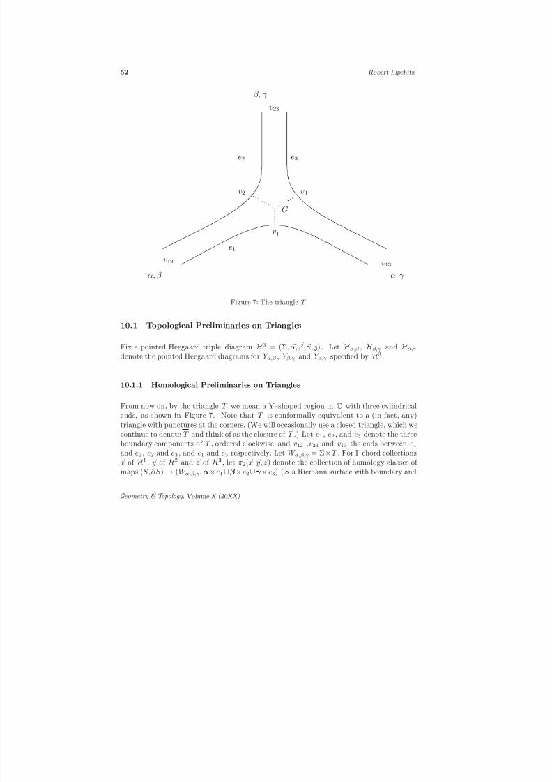
8/3/2019 Robert Lipshitz- A Cylindrical Reformulation of Heegaard Floer Homology
http://slidepdf.com/reader/full/robert-lipshitz-a-cylindrical-reformulation-of-heegaard-floer-homology 52/135
52 Robert Lipshitz
e2
v1
v2 v3
G
v12
α, γ α, β
v13
β, γ
v23
e1
e3
Figure 7: The triangle T
10.1 Topological Preliminaries on Triangles
Fix a pointed Heegaard triple–diagram H3 = (Σ, α, β, γ, z). Let Hα,β , Hβ,γ and Hα,γ
denote the pointed Heegaard diagrams for Y α,β , Y β,γ and Y α,γ specified by H3 .
10.1.1 Homological Preliminaries on Triangles
From now on, by the triangle T we mean a Y–shaped region in C with three cylindricalends, as shown in Figure 7. Note that T is conformally equivalent to a (in fact, any)
triangle with punctures at the corners. (We will occasionally use a closed triangle, which wecontinue to denote T and think of as the closure of T .) Let e1 , e2 , and e3 denote the threeboundary components of T , ordered clockwise, and v12 ,v23 and v13 the ends between e1
and e2 , e2 and e3 , and e1 and e3 respectively. Let W α,β,γ = Σ×T . For I–chord collectionsx of H1 , y of H2 and z of H3 , let π2(x, y, z) denote the collection of homology classes of maps (S,∂S ) → (W α,β,γ ,α× e1 ∪β× e2 ∪γ × e3) (S a Riemann surface with boundary and
Geometry & T opology , Volume X (20XX)

8/3/2019 Robert Lipshitz- A Cylindrical Reformulation of Heegaard Floer Homology
http://slidepdf.com/reader/full/robert-lipshitz-a-cylindrical-reformulation-of-heegaard-floer-homology 53/135
8/3/2019 Robert Lipshitz- A Cylindrical Reformulation of Heegaard Floer Homology
http://slidepdf.com/reader/full/robert-lipshitz-a-cylindrical-reformulation-of-heegaard-floer-homology 54/135

8/3/2019 Robert Lipshitz- A Cylindrical Reformulation of Heegaard Floer Homology
http://slidepdf.com/reader/full/robert-lipshitz-a-cylindrical-reformulation-of-heegaard-floer-homology 55/135

8/3/2019 Robert Lipshitz- A Cylindrical Reformulation of Heegaard Floer Homology
http://slidepdf.com/reader/full/robert-lipshitz-a-cylindrical-reformulation-of-heegaard-floer-homology 56/135
56 Robert Lipshitz
x
a
b
c
ℓα,β(t)
0 ← t e1
e2e3
t → 1v12
v23
v13
Figure 8: Foliation of T
(2) For all but finitely many t, F ∩ ℓα,β (t) consists of g + 1 disjoint embedded arcs.(3) In some small neighborhood of the corner v12 (respectively v23 , v13) of T , φ agrees
with x × T ⊂ Σ × T (respectively y × T ⊂ Σ × T , z × T ⊂ Σ × T ).
(4) The intersections F ∩π−1T (a), F ∩π−1
T (b) and F ∩π−1T (c) each consist of g +1 disjoint
embedded arcs.
(5) The preimage under φ of αi × e1 , β i × e2 and γ i × e3 is a connected arc for each i.
Such φ exist.
Fix a t such that F ∩ ℓα,β (t) consists of g +1 disjoint embedded arcs. Observe that ℓα,β (t)is diffeomorphic to Y α,β . For an appropriate choice of the height functions f α and f β , they
and a parameter for the interval ℓα,β (t) determine a Morse function f t on Y α,β . For anappropriate choice of metric, the 2–plane field L is the orthogonal complement of ∇f t . Aswhen we associated SpinC–structures on 3–manifolds to intersection points, one can thenuse the (g + 1)–tuple of paths F ∩ ℓα,β (t) to replace L with a 2–plane field defined on allof ℓα,β (t).
Doing this construction uniformly in t, we can extend L over all of ℓα,β (t) for all t such
Geometry & T opology , Volume X (20XX)

8/3/2019 Robert Lipshitz- A Cylindrical Reformulation of Heegaard Floer Homology
http://slidepdf.com/reader/full/robert-lipshitz-a-cylindrical-reformulation-of-heegaard-floer-homology 57/135
8/3/2019 Robert Lipshitz- A Cylindrical Reformulation of Heegaard Floer Homology
http://slidepdf.com/reader/full/robert-lipshitz-a-cylindrical-reformulation-of-heegaard-floer-homology 58/135
58 Robert Lipshitz
It would be nice to have a better way of presenting the construction of a SpinC–structure
on X α,β,γ from an element of π2(x, y, z). Unfortunately I do not know one.
The following is [21, Proposition 8.4]:
Lemma 10.6 The assignment described above induces a well–defined map sz : π2(x, y, z) →SpinC(X α,β,γ ).
Proof. By the previous lemma, the construction depends only on the restriction of φ to∂S . This restriction is defined up to isotopy by the element in π2(x, y, z). It is clear fromthe construction that an isotopy of φ does not change the SpinC–structure constructed.2
For s ∈ SpinC
(X α,β,γ ) we shall often write A ∈ s to mean that sz(A) = s.
Definition 10.7 Given two triples of intersection points (x, y, z) and (x′, y′, z′), andA ∈ π2(x, y, z), A′ ∈ π2(x′, y′, z′) define ψ and ψ′ to be SpinC–equivalent if there existelements Bα,β ∈ π2(x, x′), Bβ,γ ∈ π2(y, y′), and Bα,γ ∈ π2(z, z′) such that A + Bα,β +Bβ,γ + Bα,γ = A′ . We let S α,β,γ denote the set of SpinC–equivalence classes of triangles.
The following is [21, Proposition 8.5]:
Lemma 10.8 The assignment π2(x, y, z) → SpinC(X α,β,γ ) defined above descends to a map sz : S α,β,γ → SpinC(X α,β,γ ). This new map is injective. The image of sz consists of all SpinC–structures whose restrictions to ∂X α,β,γ are represented by intersection points.
Proof. Our proof is the same as in [21].
The fact that sz descends to S α,β,γ follows from the fact that the restriction of the 2–plane field used to define sz(A) to Y α,β is homologous to the 2–plane field used to define sz(x) (and similarly for the restrictions to Y β,γ and Y α,γ ). That is, suppose A and A′ areSpinC–equivalent elements of π2(x, y, z), A′ = A + Bα,β + Bβ,γ + Bα,γ . Let ξA and ξA′
denote the 2–plane fields constructed above to define sz(A) and sz(A′) respectively. We canassume that ξA and ξA′ agree outside some collar neighborhood U of ∂W α,β,γ . Further,on Y α,β × [0, 1) ⊂ U (respectively Y β,γ × [0, 1) ⊂ U , Y α,γ × [0, 1) ⊂ U ) we can assumethat ξA and ξA′ are given by ∇f ⊥α,β (respectively ∇f ⊥β,γ , ∇f ⊥α,γ ) for some Morse function
f α,β on Y α,β (respectively f β,γ on Y β,γ , f α,γ on Y α,γ ) outside some ball neighborhoods of (x ∪ z) × [0, 1) (respectively ( y ∪ z) × [0, 1), (z ∪ z) × [0, 1)). But it is then immediate fromthe definition that ξA and ξA′ define the same SpinC–structure on X α,β,γ .
Recall that the restriction map SpinC(X α,β,γ ) → SpinC(∂X α,β,γ ) commutes with the (tran-sitive) actions of H 2(X α,β,γ ) and H 2(∂X α,β,γ ) respectively. It follows that the cokernelSpinC(∂X α,β,γ )/SpinC(X α,β,γ ) is naturally identified with the cokernel of the restriction
Geometry & T opology , Volume X (20XX)
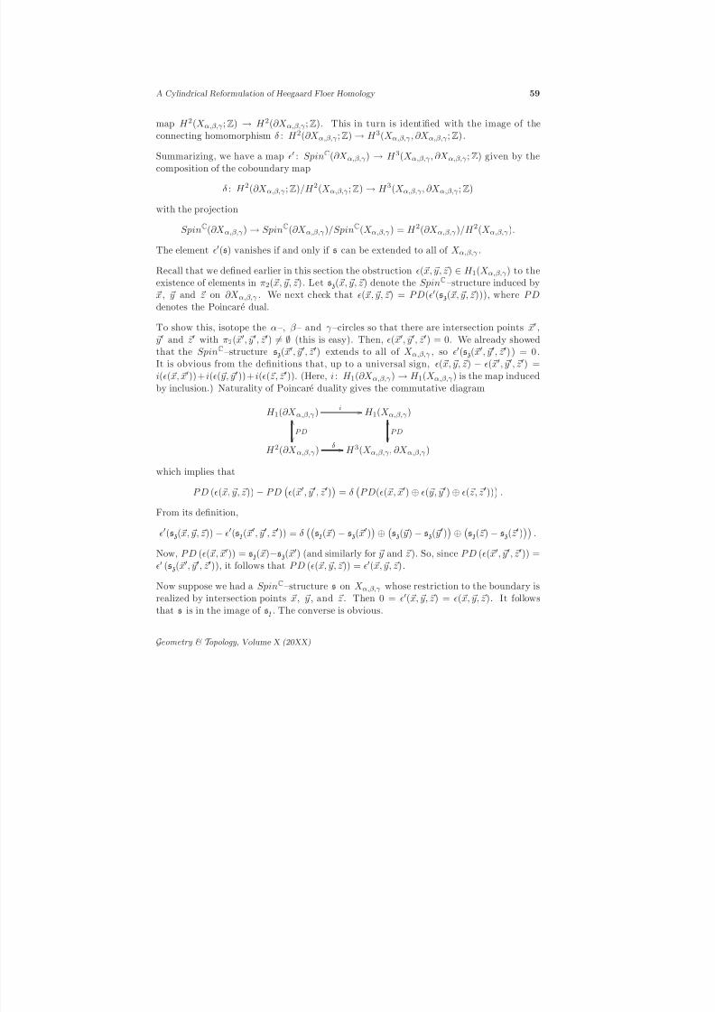
8/3/2019 Robert Lipshitz- A Cylindrical Reformulation of Heegaard Floer Homology
http://slidepdf.com/reader/full/robert-lipshitz-a-cylindrical-reformulation-of-heegaard-floer-homology 59/135
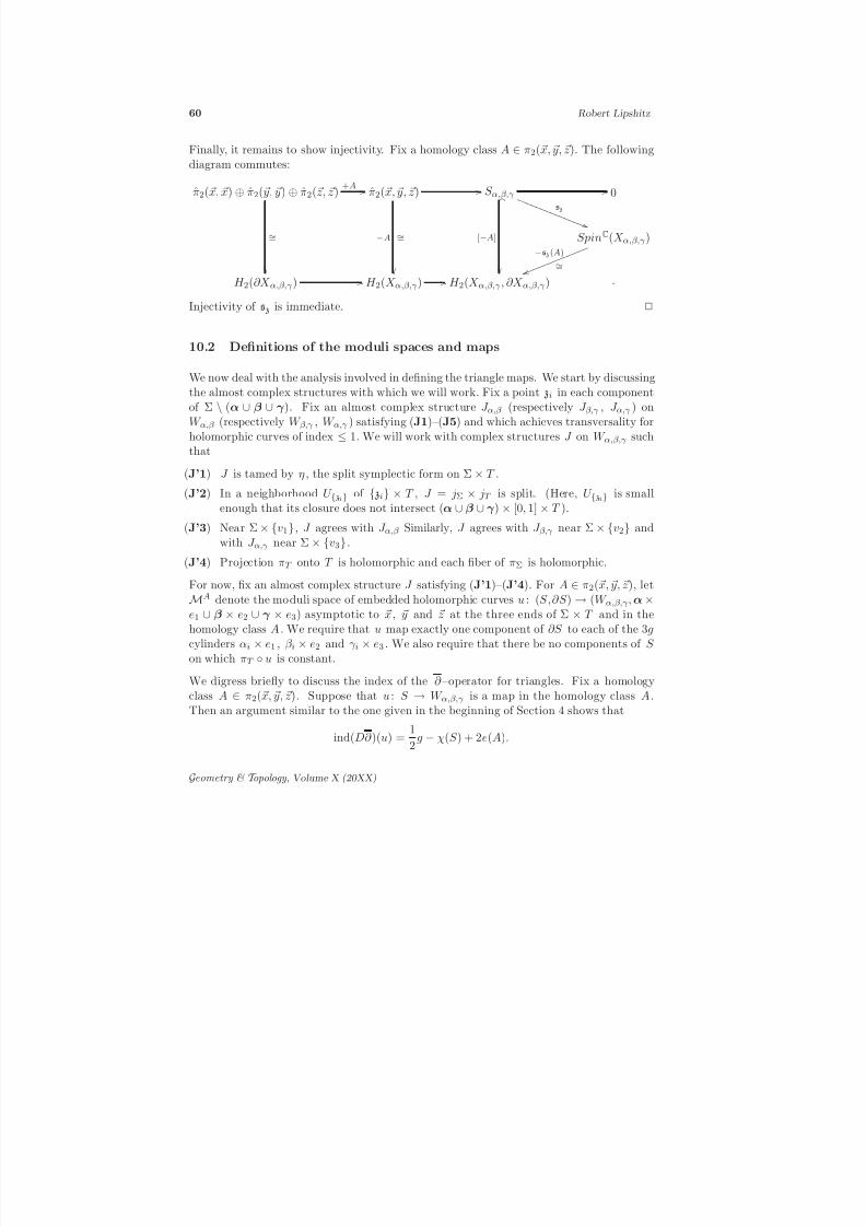
8/3/2019 Robert Lipshitz- A Cylindrical Reformulation of Heegaard Floer Homology
http://slidepdf.com/reader/full/robert-lipshitz-a-cylindrical-reformulation-of-heegaard-floer-homology 60/135
60 Robert Lipshitz
Finally, it remains to show injectivity. Fix a homology class A ∈ π2(x, y, z). The following
diagram commutes:
π2(x, x) ⊕ π2(y, y) ⊕ π2(z, z)
∼=
+A / / π2(x, y, z)
∼=−A
/ / S α,β,γ / /
sz
) ) R R R R R
R R R R R R
R R R R _
[−A]
0
SpinC(X α,β,γ )
∼=
−sz(A)
u u l l l l l
l l l l l
l l l
H 2(∂X α,β,γ ) / / H 2(X α,β,γ ) / / H 2(X α,β,γ , ∂X α,β,γ ) .
Injectivity of sz is immediate. 2
10.2 Definitions of the moduli spaces and maps
We now deal with the analysis involved in defining the triangle maps. We start by discussingthe almost complex structures with which we will work. Fix a point zi in each componentof Σ \ (α ∪ β ∪ γ ). Fix an almost complex structure J α,β (respectively J β,γ , J α,γ ) onW α,β (respectively W β,γ , W α,γ ) satisfying (J1)–(J5) and which achieves transversality forholomorphic curves of index ≤ 1. We will work with complex structures J on W α,β,γ suchthat
(J’1) J is tamed by η , the split symplectic form on Σ × T .
(J’2) In a neighborhood U zi of zi × T , J = jΣ × jT is split. (Here, U zi is smallenough that its closure does not intersect (α ∪ β ∪ γ ) × [0, 1] × T ).
(J’3) Near Σ × v1, J agrees with J α,β Similarly, J agrees with J β,γ near Σ × v2 andwith J α,γ near Σ × v3.
(J’4) Projection πT onto T is holomorphic and each fiber of πΣ is holomorphic.
For now, fix an almost complex structure J satisfying (J’1)–(J’4). For A ∈ π2(x, y, z), letMA denote the moduli space of embedded holomorphic curves u : (S,∂S ) → (W α,β,γ ,α ×e1 ∪ β × e2 ∪ γ × e3) asymptotic to x, y and z at the three ends of Σ × T and in thehomology class A. We require that u map exactly one component of ∂S to each of the 3gcylinders αi × e1 , β i × e2 and γ i × e3 . We also require that there be no components of S
on which πT u is constant.We digress briefly to discuss the index of the ∂ –operator for triangles. Fix a homologyclass A ∈ π2( x, y, z). Suppose that u : S → W α,β,γ is a map in the homology class A.Then an argument similar to the one given in the beginning of Section 4 shows that
ind(D∂ )(u) =1
2g − χ(S ) + 2e(A).
Geometry & T opology , Volume X (20XX)

8/3/2019 Robert Lipshitz- A Cylindrical Reformulation of Heegaard Floer Homology
http://slidepdf.com/reader/full/robert-lipshitz-a-cylindrical-reformulation-of-heegaard-floer-homology 61/135
A Cylindrical Reformulation of Heegaard Floer Homology 61
Here, e(A) denotes the Euler measure of A, as described in Section 4. The 12g looks
strange, but for g odd it is easy to see that 2e(A) is a half–integer. When deriving thisformula, one should keep in mind an extra −g , not appearing in Section 4, coming fromthe Maslov index of πT u.
Analogously to Subsection 4.2 we have
Proposition 10.9 The Euler characteristic of an embedded holomorphic curve u : S →W α,β,γ is determined by the homology class of u.
Proof. The only part of the index which does not depend a priori only on A is χ(S ). As inthe proof of Proposition 4.2 we will re–interpret the Euler characteristic as an intersectionnumber.
Let u : S → W α,β,γ be a holomorphic map in the homology class A. By the Riemann–Hurwitz formula, the degree of branching of πΣ u determines χ(S ), and vice versa.
Choose a diffeomorphism T → D2 \ z3 = 1 from T to the unit disk with three boundarypunctures. Let ξT be the vector field on T induced by the vector field r ∂
∂θ on D2 . Here,
we choose the diffeomorphism so that the preimage of 0 is not a branch point of πT u.Let ξ be the vector field 0 × ξT on W α,β,γ . Then, for ǫ small, the degree of branching of πΣ u is given by #(u ∩ expǫξ(u)) − g .
Fix embedded holomorphic curves u : S → W α,β,γ , u′ : S ′ → W α,β,γ in the homologyclass A. Because we are in a low dimension (two), we can choose a (proper) bordism
v : R → W α,β,γ from u to u′
. Choose a Morse function f : R →R
with ∂R = f −1
(0, 1),and so that v restricts to u on f −1(0) and to u′ on f −1(1). We will think of f as acoordinate on R, and write Ra for f −1(a) and va = v|Ra .
For an appropriate choice of R, v and f there is a partition 0 = t0 < s1 < t1 < s2 < t2 <· · · < sk = 1 of [0, 1] such that
• The function f has no critical values in [si, ti], i = 1, · · · k (and so f −1([si, ti]) is aproduct).
• For each point si (respectively ti), vsi (respectively vti ) is an embedding in thehomology class A which projects as a branched cover to T .
• The map v|f −1((ti,si+1)) is constant near infinity (as a function of f ( p)).
In words, we have chosen R, v and f so that we can subdivide [0, 1] into subintervalsover which either the map doesn’t change near the punctures or the topology of S doesn’tchange near the punctures (and so that each interval starts and ends with maps for whichthe degree of branching of πΣ va determines χ(Ra)).
For each i, χ(Rsi) = χ(Rti), by the first property.
Geometry & T opology , Volume X (20XX)
8/3/2019 Robert Lipshitz- A Cylindrical Reformulation of Heegaard Floer Homology
http://slidepdf.com/reader/full/robert-lipshitz-a-cylindrical-reformulation-of-heegaard-floer-homology 62/135
62 Robert Lipshitz
Also, if a, a′, a′′ ∈ (ti, si+1) are regular values then #(va ∩ va′) = #(va ∩ va′′). It follows
from the Riemann–Hurwitz formula that χ(Rti) = χ(Rti+1).But this implies that χ(S ) = χ(Rt0) = χ(Rsk) = χ(S ′), completing the proof. 2
For A ∈ π2(x, y, z), let ind(A) denote the index of the D∂ problem for embedded curvesin the homology class A, if such an embedded curve exists. Note that the index is additivein the sense that for Bα,β ∈ π2(x, x′), ind(A + Bα,β ) = ind(A) + ind(Bα,β ) (and similarlyfor the other ends), if b oth sides are defined. We shall omit the words “if defined” fromall subsequent discussion of the index – that we are only discussing homology classesrepresentable by holomorphic curves will be implicit throughout.
Remark. We could have proved Proposition 10.9 in more generality by using an analogof Lemma 4.1. Then, ind(A) would have a natural meaning for any homology class A ∈
π2(x, y, z). The only cases in which we are interested in the index, however, are when thereis an embedded holomorphic curve.
We now must check that, for generic J satisfying (J’1)–(J’4), the moduli spaces of J –holomorphic curves MA are reasonably well behaved. Again, we achieve transversality byvarying J . The argument to show that one can achieve transversality among J satisfying(J’1)–(J’4) is analogous to the one given in Section 3.
Note that bubbling and Deligne–Mumford type degenerations in moduli spaces with ind ≤1 are prohibited by the argument used in Section 7. So, by the compactness theorem [2,Theorem 10.2], the compactification of MA consists of holomorphic buildings with onestory in W α,β,γ and all of their other stories in W α,β , W β,γ or W α,γ . (As is standard in
symplectic field theory, the stories in the cylindrical bordisms W α,β , W β,γ , and W α,γ areonly defined up to translation.)
For the rest of this section, fix a SpinC equivalence class of triangles. Denote it sα,β,γ . Fixa complex structure satisfying (J’1)–(J’4) and achieving transversality.
There are still some technical details to address before we can define the triangle maps.However, we will give the definitions now, asking the reader to trust that all the symbolsmake sense and sums are finite. We will justify this trust presently.
Given the choice of sα,β,γ ∈ SpinC(X α,β,γ ) we will define a map
f ∞α,β,γ : CF ∞(Y α,β ) ⊗Z[U ] CF ∞(Y β,γ ) → CF ∞(Y α,γ )
by
f ∞α,β,γ ([x, i] ⊗ [y, j]) =z
A∈π2(x, y,z)∩sα,β,γ
ind(A)=0
#MA [z, i + j − nz(A)].
Remark. For the complexes CF ∞ , CF − , CF + and CF ≤0 our tensor products shall alwaysbe over Z[U ]. For CF they shall be over Z . In the case of CF ∞ it would be equivalent to
Geometry & T opology , Volume X (20XX)
8/3/2019 Robert Lipshitz- A Cylindrical Reformulation of Heegaard Floer Homology
http://slidepdf.com/reader/full/robert-lipshitz-a-cylindrical-reformulation-of-heegaard-floer-homology 63/135
8/3/2019 Robert Lipshitz- A Cylindrical Reformulation of Heegaard Floer Homology
http://slidepdf.com/reader/full/robert-lipshitz-a-cylindrical-reformulation-of-heegaard-floer-homology 64/135
64 Robert Lipshitz
MBα,β(Y α,β ), MBβ,γ (Y β,γ ) and MBα,γ(Y α,γ ) (or rather, for the determinant line bundles
over the corresponding configuration spaces) which are consistent with gluings. However,we would like somewhat more. Specifically
Lemma 10.10 Given coherent orientation systems oα,β (Bα,β ) and oβ,γ (Bβ,γ ) (for all Bα,β and Bβ,γ ) there are orientation systems oα,γ and oα,β,γ consistent with oα,β andoβ,γ . (Compare [21, Lemma 8.7].)
Note that we have not claimed that oα,γ and oα,β,γ are unique. The indeterminacy will beclear from the proof.
Proof of Lemma 10.10. Our proof is the same as in [21, Section 8.2].
Fix a SpinC–structure sα,β,γ on X α,β,γ and intersection points x0 ∈ sα,β,γ |Y α,β , y0 ∈ sα,β,γ |Y β,γ and z0 ∈ sα,β,γ |Y α,γ . Fix A0 ∈ π2( x0, y0, z0). Choose any orientation over A0 .
Let
K = Bα,γ ∈ π2(z0, z0) | ∃Bα,β ∈ π2(x0, x0), Bβ,γ ∈ π2(y0, y0)
such that A0 + Bα,γ = A0 + Bβ,γ + Bα,γ .
Sublemma 10.11 (1) π2(z0, z0) ∼= K ⊕ ZN for some N .
(2) Given Bα,γ ∈ K there is only one pair Bβ,γ , Bα,γ such that A0 + Bα,γ = A0 + Bβ,γ +
Bα,γ .
Assuming the sublemma, the lemma is almost immediate. By Part 2 of the sublemma,oα,β,γ (A0), oα,β , and oβ,γ determine oα,γ over K . Choosing oα,γ arbitrarily over a basis of ZN determines oα,γ over π2(z0, z0). The orientation over [Σ] is determined as in Section 6.
Choosing a homology class Bα,γ,z ∈ π2(z0, z) for each intersection point z (i.e., a completeset of paths for Y α,γ in the sense of Section 6) and then choosing orientations arbitrarilyover the Bα,γ,z determines oα,γ over all of sα,β,γ |Y α,γ . The orientation over A0 and oα,β ,oβ,γ and oα,γ together determine oα,β,γ over all of sα,β,γ . This completes the proof, exceptfor the
Proof of Sublemma 10.11. The subgroup K is canonically identified with the intersectionof H 2(Y α,β ∪ Y β,γ ) and H 2(Y α,γ ) in H 2(X α,β,γ ). From the fragment
H 3(X α,β,γ , Y α,β ∪ Y β,γ ) → H 2(Y α,β ∪ Y β,γ )j
→ H 2(X α,β,γ )p
→ H 2(X α,β,γ , Y α,β ∪ Y β,γ )
of the long exact sequence for the pair (X α,β,γ , Y α,β ∪ Y β,γ ), one sees π2(z0, z0)/K ∼= p i(H 2(Y α,γ )). By excision, H ∗(X α,β,γ , Y α,β ∪ Y β,γ ) ∼= H ∗(U β × [0, 1], U β × ∂ [0, 1]). So,
Geometry & T opology , Volume X (20XX)
8/3/2019 Robert Lipshitz- A Cylindrical Reformulation of Heegaard Floer Homology
http://slidepdf.com/reader/full/robert-lipshitz-a-cylindrical-reformulation-of-heegaard-floer-homology 65/135
8/3/2019 Robert Lipshitz- A Cylindrical Reformulation of Heegaard Floer Homology
http://slidepdf.com/reader/full/robert-lipshitz-a-cylindrical-reformulation-of-heegaard-floer-homology 66/135
66 Robert Lipshitz
Note that weak (respectively strong) admissibility for H3 implies weak (strong) admissi-
bility for each of Hα,β , Hβ,γ and Hα,γ .
The proof of the following alternate characterization of weak admissibility is the same asthe proof of Lemma 5.3.
Lemma 10.14 With notation as above,
• The diagram H3 is weakly admissible if and only if there is an area form on Σwith respect to which for any Bα,β , Bβ,γ and Bα,γ as in the definition of weak admissibility, the domain Bα,β + Bβ,γ + Bα,γ has zero signed area.
• The diagram H3 is strongly admissible for s if there is an area form on Σ with respectto which for any Bα,β , Bβ,γ and Bα,γ as in the definition of strong admissibility,
Bα,β + Bβ,γ + Bα,γ has signed area equal to n, and with respect to which Σ has area 1.
Recall that we call a homology class A positive if the corresponding domain has no negativecoefficients.
The following is [21, Lemma 8.9]
Lemma 10.15 Suppose H3 is weakly admissible. Fix intersection points x , y , and zand a SpinC–structure s on X α,β,γ . Then for each j, k ∈ Z there are only finitely many positive A ∈ sα,β,γ ∩ π2(x, y, z) such that
• ind(A) = j ,
• nz(A) = k ,
Proof. Suppose that A, A′ ∈ π2(x, y, z), nz(A) = nz(A′) = k , and A, A′ ∈ sα,β,γ . Thenby Lemma 10.8, A and A′ are SpinC–equivalent, so A′ = A + Bα,β + Bβ,γ + Bα,γ whereBα,β ∈ π2(x, x), Bβ,γ ∈ π2(y, y), and Bα,γ ∈ π2(z, z). By the previous lemma, we canchoose an area form on Σ so that Bα,β + Bβ,γ + Bα,γ has zero signed area. The result thenfollows as in Lemma 5.4. 2
It follows from this lemma and compactness that if H3 satisfies the weak admissibilitycriterion then the sums defining f α,β,γ and f +
α,β,γ
are finite.
The following is [21, Lemma 8.10].
Lemma 10.16 Fix j ∈ Z, intersection points x, y , z , and a SpinC–structure sα,β,γ .Suppose H3 is strongly admissible for s. Then there are only finitely many positive A ∈π2(x, y, z) ∩ sα,β,γ such that ind(A) = j .
Geometry & T opology , Volume X (20XX)
8/3/2019 Robert Lipshitz- A Cylindrical Reformulation of Heegaard Floer Homology
http://slidepdf.com/reader/full/robert-lipshitz-a-cylindrical-reformulation-of-heegaard-floer-homology 67/135
A Cylindrical Reformulation of Heegaard Floer Homology 67
Proof. As in the previous proof, given A, A′ ∈ π2(x, y, z) satisfying the hypotheses,
A − A′ = Bα,β + Bβ,γ + Bα,γ for some Bα,β ∈ π2(x, x), Bβ,γ ∈ π2(y, y) and Bα,γ ∈ π2(z, z).The proof then follows as in Lemma 5.5. 2
It follows from this lemma and compactness that if H3 satisfies the strong admissibilitycriterion then the sums defining f ∞α,β,γ and f ≤0
α,β,γ are finite.
The following is [21, Lemma 8.11]. We refer the reader there for its proof.
Proposition 10.17 Given any pointed Heegaard triple–diagram (Σ, α, β, γ, z) there is anisotopic weakly admissible Heegaard triple–diagram. Given any pointed Heegaard triple– diagram (Σ, α, β, γ, z) and a SpinC–structure sα,β,γ on X α,β,γ there is an isotopic pointedHeegaard triple–diagram which is strongly admissible for sα,β,γ .
10.5 Moduli spaces and maps, part 2.
If we wish to make a statement about all of f ∞α,β,γ , f ≤0α,β,γ , f +α,β,γ , or f α,β,γ at once we will
simply write f α,β,γ . For example
Lemma 10.18 The maps f α,β,γ are chain maps.
Proof. This follows by considering the 1–dimensional moduli spaces MAα,β,γ whereAα,β,γ ∈ π2(x, y, z), ind(Aα,β,γ ) = 1. The proof of Proposition 7.1 still works, so theboundary of MAα,β,γ consists of height two holomorphic buildings in the homology classAα,β,γ . Each of of these height two holomorphic buildings consists of
(1) a curve of index 0 in Σ × T and
(2) a curve of index 1 (defined up to translation) in one of W α,β , W β,γ or W γ,α ,
and every such building is in ∂ MAα,β,γ for some Aα,β,γ of index 1. This follows from [2,Theorem 10.2] and Proposition A.1. Hence,
0 = #
∂ MC
=
Bα,β∈π2(x,x′)
ind(Bα,β)=1
# MBα,β
#MAα,β,γ−Bα,β
+
Bβ,γ∈π2( y, y′)
ind(Bβ,γ )=1
#
MBβ,γ
#MAα,β,γ−Bβ,γ
+
Bα,γ∈π2(z′,z)ind(Bα,γ)=1
# MB
α,γ
#MAα,β,γ−Bα,γ
.
But summing this over Aα,β,γ with nz(Aα,β,γ ) = k gives the coefficient of [z, i + j − k] in∂ f ∞α,β,γ + f ∞α,β,γ ∂ , proving the result for f ∞α,β,γ .
Geometry & T opology , Volume X (20XX)
8/3/2019 Robert Lipshitz- A Cylindrical Reformulation of Heegaard Floer Homology
http://slidepdf.com/reader/full/robert-lipshitz-a-cylindrical-reformulation-of-heegaard-floer-homology 68/135
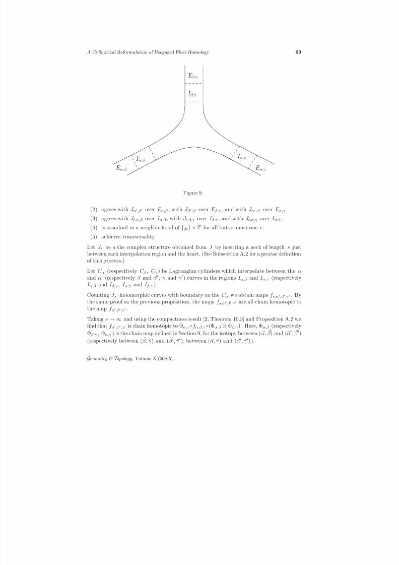
8/3/2019 Robert Lipshitz- A Cylindrical Reformulation of Heegaard Floer Homology
http://slidepdf.com/reader/full/robert-lipshitz-a-cylindrical-reformulation-of-heegaard-floer-homology 69/135
8/3/2019 Robert Lipshitz- A Cylindrical Reformulation of Heegaard Floer Homology
http://slidepdf.com/reader/full/robert-lipshitz-a-cylindrical-reformulation-of-heegaard-floer-homology 70/135
70 Robert Lipshitz
Orientation systems, which have been implicit in the discussion, are extended as discussed
in Section 9. 2
10.6 Associativity of triangle maps.
Next we show that the maps F α,β,γ satisfy an associativity property. Before stating it,however, we need some basic properties of Heegaard quadruple–diagrams.
10.6.1 Heegaard quadruple–diagrams.
As the reader can presumably guess, a pointed Heegaard quadruple–diagram consists of a
genus g surface Σ, four g–tuples of pairwise disjoint homologically linearly independentsimple closed curves α, β , γ and δ , and a distinguished point z ∈ Σ\(α∪β∪γ ∪δ). In thissection we will state the analogs for Heegaard quadruple–diagrams of the basic definitionsand lemmas stated earlier for Heegaard triple diagrams. Except as noted, the proofs arethe same as for Heegaard triple–diagrams, and hence are omitted.
Fix a pointed Heegaard quadruple–diagram H4 = (Σ, α, β, γ, δ, z). The diagram H4 speci-fies a 4–manifold X α,β,γ,δ with boundary ∂X α,β,γ,δ = Y α,β ∪ Y β,γ ∪ Y γ,δ ∪ (−Y α,δ) by gluingthe elongated handlebodies U α× [0, 1], U β × [0, 1], U γ × [0, 1] and U δ × [0, 1] to the productof Σ and a square.
Let W α,β,γ,δ be the product of Σ and a disk R with four boundary punctures, thought of asa topological space without complex structure for the moment. Let e1, · · · , e4 denote thefour boundary arcs of R, enumerated clockwise, v12 , v23 , v34 and v41 the four punctures,with vij between ei and e j ; see Figure 10. In W α,β,γ,δ we have 4g cylinders: α × e1 ,β × e2 , γ × e3 and δ × e4 . Let π2(x, y, z, w) denote the collection of homology classes of maps (S,∂S ) → (W α,β,γ,δ ,α× e1 ∪ · · · ∪ δ × e4) asymptotic to the I–chord collection x forHα,β at v1 , y for Hβ,γ at v2 , and so on.
Given x, · · · , w there is an element ǫ(x, y, z, w) ∈ H 1(X α,β,γ,δ) defined as we definedǫ(x, y, z) for triangles in Subsection 10.1.
Lemma 10.21 (1) π2(x, y, z, w) is nonempty if and only if ǫ(x, y, z, w) = 0.
(2) If ǫ(x, y, z, w) = 0 then π2(x, y, z, w) ∼= Z⊕H 2(X α,β,γ,δ). The map π2(x, y, z, w) → Z
is given by nz. The identification of π2( x, y, z, w)/Z with H 2(X α,β,γ,δ) is affine (butcanonical up to translation).
Proof. See Lemma 10.2 and Lemma 10.3. 2
As with triangles, each element A of π2(x, y, z, w) specifies a SpinC–structure sz(A) onX α,β,γ,δ ; the construction is the same as in Subsubsection 10.1.2. Also as before, there are
Geometry & T opology , Volume X (20XX)
8/3/2019 Robert Lipshitz- A Cylindrical Reformulation of Heegaard Floer Homology
http://slidepdf.com/reader/full/robert-lipshitz-a-cylindrical-reformulation-of-heegaard-floer-homology 71/135

8/3/2019 Robert Lipshitz- A Cylindrical Reformulation of Heegaard Floer Homology
http://slidepdf.com/reader/full/robert-lipshitz-a-cylindrical-reformulation-of-heegaard-floer-homology 72/135
72 Robert Lipshitz
• ξ,η Bξ,η = 0 and
• ξ,η c1 sα,β,γ |Y ξ,η , Bξ,η = 2n ≥ 0
then some coefficient of
ξ,η Bξ,η is greater than n.
Lemma 10.25 (1) Given any pointed Heegaard quadruple–diagram there is an isotopic weakly admissible pointed Heegaard quadruple–diagram.
(2) Suppose that the pointed Heegaard quadruple–diagram (Σ, α, β, γ, δ, z) satisfies the conditions δβ,δH 1(Y β,δ)|Y α,γ = 0 and δα,γ H 1(Y α,γ )|Y β,δ = 0. Fix a δα,γ H 1(Y α,γ ) +
δβ,δH 1(Y β,δ)–orbit of SpinC–structures S. Then there is an isotopic pointed Hee-gaard quadruple–diagram which is strongly admissible for S.
For the argument, see [21, Section 8.4.2].
Lemma 10.26 Suppose H4 is weakly admissible. Fix j, k ∈ Z, intersection points x, y, z, w and a δH 1(Y β,δ) + δH 1(Y α,γ )–orbit of SpinC–structures S on X α,β,γ,δ . Thenthere are only finitely many positive A ∈ π2(x, y, z, w) such that
• ind(A) = j
• nz(A) = k
• sz(A) ∈ S
Proof. See Lemma 10.15. 2
Lemma 10.27 Suppose H4 is strongly admissible for a δα,γ H 1(Y α,γ ) + δβ,δH 1(Y β,δ)– orbit of SpinC–structures S on X α,β,γ,δ . Fix j ∈ Z and intersection points x, y, z, w .Then there are only finitely many positive A ∈ π2(x, y, z, w) such that sz(A) ∈ S andind(A) = j .
Proof. See Lemma 10.16. 2
10.6.2 Moduli spaces of squares
Fix a pointed Heegaard quadruple–diagram H4 = (Σ, α, β, γ, δ, z). Let R denote the unit
disk with four punctures on its boundary. Let e1, · · · , e4 denote the four boundary compo-nents of R, enumerated clockwise, and v12, v23, v34 and v4,1 the vertices of R, enumeratedclockwise, with v12 between e1 and e2 . See Figure 10. Let W α,β,γ,δ = Σ × R.
The moduli space of conformal structures on a rectangle is parameterized by R. Let ja ,a ∈ R, sweep out this space. Do this in such a way that as s → −∞ an arc in R connectinge1 to e3 collapses, while as s → ∞ an arc in R connecting e2 to e4 collapses; see Figure 10.
Geometry & T opology , Volume X (20XX)
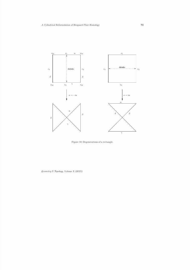
8/3/2019 Robert Lipshitz- A Cylindrical Reformulation of Heegaard Floer Homology
http://slidepdf.com/reader/full/robert-lipshitz-a-cylindrical-reformulation-of-heegaard-floer-homology 73/135
A Cylindrical Reformulation of Heegaard Floer Homology 73
shrinksshrinks
e1
e2
e3
e4
v12
v23v34
s→−∞ s→∞
v41 α
β
γ
δ
α
β
δ
δ
α
γ
β
γ
e1
e2
e3
e4
Figure 10: Degenerations of a rectangle.
Geometry & T opology , Volume X (20XX)
8/3/2019 Robert Lipshitz- A Cylindrical Reformulation of Heegaard Floer Homology
http://slidepdf.com/reader/full/robert-lipshitz-a-cylindrical-reformulation-of-heegaard-floer-homology 74/135
74 Robert Lipshitz
Fix a point zi in each component of Σ \ (α ∪ β ∪ γ ∪ δ). Choose complex structures J ξ,η ,
ξ, η ⊂ α ,β ,γ ,δ which satisfy (J1)–(J5) and achieve transversality.
Fix a path J a of complex structures on W α,β,γ,δ such that
(1) For every a ∈ R, J a is tamed by the split symplectic form on Σ × R.
(2) For every a ∈ R, projection πR onto R is ( ja, J a)–holomorphic.
(3) In a neighborhood U zi of zi × R, J = jΣ × jT is split.
(4) Near Σ × v12, J agrees with J α,β . Near Σ × v23, J agrees with J β,γ . NearΣ × v34, J agrees with J γ,δ . Near Σ × v41, J agrees with J α,δ .
(5) As a → −∞, J a degenerates to complex structures which satisfy (J’1)–(J’4) andachieve transversality for W α,β,γ and W α,γ,δ .
(6) As a → ∞, J a degenerates to complex structures which satisfy (J’1)–(J’4) andachieve transversality for W δ,α,β and W γ,δ,β .
(7) J a achieves transversality (as a path of almost complex structures) for holomorphiccurves with index ≤ 1.
Checking that such a J a exists is similar to the proof of transversality in Section 3.
Given I–chord collections x, y, z, w for Y α,β , Y β,γ , Y γ,δ and Y α,δ we let π2(x, y, z, w) denotehomology classes of maps to W α,β,γ,δ connecting x, y , z , and w . Given A ∈ π2( x, y, z, w),let MA denote the union over a ∈ R of all embedded J a–holomorphic curves u : (S,∂S ) →(W α,β,γ,δ ,α × e1 ∪ β × e2 ∪ γ × e3 ∪ δ × e4) (without closed components, and with onecomponent of ∂S mapped to each Lagrangian cylinder) in the homology class A. Let
ind(A) denote the index of this ∂ problem in the homology class A, so dimMA
= ind(A)+1, if MA is nonempty. (The +1 appears because we consider a 1–parameter family of almost complex structures.)
10.6.3 Orienting squares
The moduli spaces MAα,β,γ,δ are orientable for the same reason all the other moduli spacesconsidered so far have been. Again we want to choose orientations for the MAα,β,γ,δ ,MAκ,η,ξ and MBη,ξ , κ,η,ξ ⊂ α ,β ,γ ,δ) consistent with various gluings – all possiblegluings of a 2–gon to a rectangle or triangle, and the two gluings MAα,β,γ × MAα,γ,δ ×[R, ∞) → MAα,β,γ+Aα,γ,δ and MAα,β,δ × MAβ,γ,δ × [R, ∞) → MAα,β,δ+Aβ,γ,δ . Again, it
follows from standard arguments that there is some such coherent orientation system.And, again it is useful to have something slightly stronger:
Lemma 10.28 Suppose H4 is a Heegaard quadruple–diagram such that the image of H 2(Y β,δ) under the map H 2(X α,β,γ,δ) → H 2(X α,β,γ,δ , ∂X α,β,γ,δ) is zero. Fix a δH 1(Y α,γ )– orbit of SpinC–structures S on X α,β,γ,δ and orientation systems oα,β,γ and oα,γ,δ for
Geometry & T opology , Volume X (20XX)
8/3/2019 Robert Lipshitz- A Cylindrical Reformulation of Heegaard Floer Homology
http://slidepdf.com/reader/full/robert-lipshitz-a-cylindrical-reformulation-of-heegaard-floer-homology 75/135
A Cylindrical Reformulation of Heegaard Floer Homology 75
(Σ, α, β, γ, z,S|Xα,β,γ) and (Σ, α, γ, δ, z,S|Xα,γ,δ
) inducing the same orientation over Y α,γ .
Then there is a coherent orientation system for H4 extending oα,β,γ and oα,γ,δ . (Com- pare [21, Proposition 8.15].)
Proof. Our proof is the same as the one given in [21].
The orientation systems oα,β,γ and oα,γ,δ determine orientations oα,β,γ,δ(Aα,β,γ,δ) for allAα,β,γ,δ with sz(Aα,β,γ,δ) ∈ S, which is well–defined since oα,β,γ and oα,γ,δ induce thesame orientation system on Y α,γ . The orientation systems oα,β,γ and oα,γ,δ also determineorientation systems oα,β , oβ,γ , oγ,δ , oα,δ and oα,γ over Y α,β , Y β,γ , Y γ,δ , Y α,δ and Y α,γ .
Choose intersection points x ∈ S|Y α,β , y ∈ S|Y β,γ , z ∈ S|Y γ,δ , w ∈ S|Y α,δ , u ∈ S|Y α,γ andv ∈ S|Y β,δ . Choose any Aα,β,γ,0 ∈ π2( x, y, u) and Aβ,γ,δ,0 ∈ π2(y, z, v). Choose an arbitrary
orientation oα,β,δ(Aα,β,δ,0) over Aα,β,δ,0 . Then oα,β,δ(Aα,β,δ,0) and oα,β,γ,δ(Aα,β,δ,0+Aβ,γ,δ,0)determine an orientation oβ,γ,δ(Aβ,γ,δ,0).
Now, we choose oβ,δ as follows. For Bβ,δ ∈ π2(v, v), from the assumption that H 2(Y β,δ) istrivial inside H 2(X α,β,γ,δ , ∂X α,β,γ,δ), we can choose Bα,β , Bβ,γ , Bγ,δ and Bα,δ so that
Aα,β,δ,0 + Aβ,γ,δ,0 + Bβ,δ = Aα,β,δ,0 + Aβ,γ,δ,0 + Bα,β + Bβ,γ + Bγ,δ + Bα,δ (10)
Choose oβ,δ(Bβ,δ) so that the orientations induced by the two decompositions in Equa-tion (10) agree. We have constructed oα,β , oβ,γ , oγ,δ and oα,δ so that this is independentof the choice of Bα,β , · · · , Bα,δ . Choose arbitrary orientations over a complete set of pathsfor Y β,δ to finish defining oβ,δ .
Finally, oα,β,δ(Aα,β,δ,0), oα,β , oβ,δ and oα,δ together specify oα,β,δ completely, and a similarremark applies to oβ,γ,δ . We have, thus, finished constructing all the orientations. It isclear that they are coherent. 2
10.6.4 Proof of associativity
Proposition 10.29 Let H4 = (Σ, α, β, γ, δ, z) be a pointed Heegaard quadruple–diagram.Fix a δα,γ H 1(Y α,γ ) + δβ,δH 1(Y β,δ )–orbit of SpinC–structures S on X α,β,γ,δ . Assume thatH4 is strongly admissible for S. Fix ∗ ∈ ∞, +, −. Then for any ξα,β ∈ HF ∗(Y α,β ) andθβ,γ ∈ HF ≤0(Y β,γ ), θγ,δ ∈ HF ≤0(Y γ,δ ) we have
s∈SF ∗
α,γ,δF ∗α,β,γ (ξα,β ⊗ θβ,γ ; s|Xα,β,γ) ⊗ θγ,δ ; s|Xα,γ,δ
=s∈S
F ∗α,β,δ
ξα,β ⊗ F ≤0
β,γ,δ(θβ,γ ⊗ θγ,δ ; s|Xβ,γ,δ); s|Xα,β,δ
.
An exactly similar statement holds with both HF ∗ and HF ≤ replaced by HF . For the case of HF , weak admissibility of the Heegaard quadruple–diagram is sufficient.
Geometry & T opology , Volume X (20XX)
8/3/2019 Robert Lipshitz- A Cylindrical Reformulation of Heegaard Floer Homology
http://slidepdf.com/reader/full/robert-lipshitz-a-cylindrical-reformulation-of-heegaard-floer-homology 76/135
76 Robert Lipshitz
(In the proposition, we assume the maps are computed with respect to a coherent choice of
orientations, as described in Subsubsection 10.6.3. Also note that every SpinC
–structurein S restricts to the same SpinC–structure on Y α,β (respectively Y β,γ , Y γ,δ , Y α,δ ). Whenwe speak of the Floer homology groups of Y α,β (respectively Y β,γ , Y γ,δ , Y α,δ ) we mean theFloer homology groups calculated with respect to this SpinC–structure.)
Proof. To make notation clearer, we will give the proof for ∗ = ∞. The other cases arecompletely analogous. Define h : CF ∞(Y α,β ) ⊗ CF ≤0(Y β,γ ) ⊗ CF ≤0(Y γ,δ) → CF ∞(Y α,δ)by
h ([ x, i] ⊗ [ y, j] ⊗ [z, k]) = w
A∈π2(x,vy,z, w)
sz(A)∈Sind(A)=−1
#MA
[ w, i + j + k − nz(A)].
The sum defining h makes sense by compactness and Lemma 10.27. Note that the map hhas degree −1.
Counting the ends of the space A∈S
ind(A)=0
MA
we find that
0 =s∈S
f ∞α,γ,δ
f ∞α,β,γ ([x, i] ⊗ [y, j]; s|Xα,β,γ) ⊗ [z, k]; s|Xα,γ,δ
−
s∈Sf ∗α,β,δ
[x, i] ⊗ f ≤0β,γ,δ([ y, j] ⊗ [z, k]; s|Xβ,γ,δ
); s|Xα,β,δ+ h ∂ ([x, i] ⊗ [y, j] ⊗ [z, k]) + ∂ h([x, i] ⊗ [y, j] ⊗ [z, k]).
(The first two terms correspond to contributions from the degenerations shown in Fig-ure 10. The last two terms correspond to the usual level splittings at the (four) cylindricalends.)
The result is immediate. 2
11 Handleslides
In this section we will prove that the Floer homologies defined in Section 8 are unchangedby handleslides among the β – (and, symmetrically, the α–) circles. This follows from theassociativity of the triangle maps defined in Section 10 and the calculation of a few specificmoduli spaces.
Our proof is essentially the same as the proof given by Ozsvath and Szabo in [21, Section9]. Indeed, their calculations are done in our language, and most of the rest of the proof
Geometry & T opology , Volume X (20XX)

8/3/2019 Robert Lipshitz- A Cylindrical Reformulation of Heegaard Floer Homology
http://slidepdf.com/reader/full/robert-lipshitz-a-cylindrical-reformulation-of-heegaard-floer-homology 77/135
A Cylindrical Reformulation of Heegaard Floer Homology 77
follows formally from the results of Section 10. Our proof differs from theirs in the follow-
ing ways. Firstly, we try to calculate the minimum amount necessary in order to provehandleslide invariance. We hope this will provide a slightly better understanding of theformal properties underlying handleslide invariance, and in turn lead to generalizations.Secondly, we give a more geometrical proof of Proposition 11.4 (roughly [21, Proposition9.8]), using 1–gons. Thirdly, some details about the H 1(Y )/Tors–actions look slightlydifferent in our language.
We now state the main steps, and then return later to the proofs. First, notation. Let H =(Σ, α, β, z) be a pointed Heegaard diagram. Let β ′i be a small Hamiltonian perturbationof β i intersecting β i transversally in two points and disjoint from β j for i = j . Let β H 1
be a curve obtained by handlesliding β 1 over β 2 in the complement of z and then doinga small isotopy so that β H
1
intersects each of β 1 and β ′
1
transversally in two points and isdisjoint from β i and β ′i for i > 1. Let β H i , i > 1, be a small Hamiltonian perturbation of β i , intersecting each of β i and β ′i transversally in two points and disjoint from β j and β ′ jfor j = i. See Figure 11. In the notation of [21, Section 9], our β ′i is their δi and our β H i
is their γ i .
There are 2g intersection points in (Σ, β, β ′, z). Let θβ,β ′ = θ1, · · · , θg denote the unique
intersection point of maximal grading. Similarly, in (Σ, β, β H , z) (respectively (Σ, β, β ′, z))there are exactly 2g intersection points. Let θβ,β H = θH 1 , · · · , θH g (respectively θβ ′,β H =θ′1, · · · , θ′g) denote the unique intersection point of maximal grading. See Figure 11.
A few words about SpinC–structures. We fix a SpinC–structure s on Y α,β for the rest of
the section; when we refer to Floer homology groups of Y α,β we mean the groups computedwith respect to s. Now, note that all of the 3·2g intersection points in (Σ, β, β ′), (Σ, β, β H )and (Σ, β ′, β H ) represent the unique torsion SpinC–structure on #gS 1 × S 2 . (This fol-lows, for instance, from Lemma 4.11.) Throughout this section, when discussing Heegaarddiagrams for #gS 1 × S 2 we shall implicitly work with the torsion SpinC–structure. Laterin this section, we shall consider the Heegaard triple–diagrams (Σ, α, β, β H ), (Σ, α, β, β ′),and (Σ, β, β H , β ′). It is easy to see that X α,β,β H and X α,β,β ′ are each diffeomorphic tothe complement of (a neighborhood of) a bouquet of g circles in Y α,β × [0, 1]. (Com-pare [21, Example 8.1].) By considering cohomology groups, say, it follows that given aSpinC–structure s on Y α,β there is a unique SpinC–structure on X α,β,β H (respectively
X α,β,β ′ ) which restricts to s on Y α,β and the torsion SpinC–structure on Y β,β H (respec-
tively Y β,β ′ ). It follows that there is a unique SpinC–structure on X β,β H ,β ′ which restrictsto the torsion SpinC–structure on the three boundary components. When discussing tri-angle maps we shall always assume that they are computed with respect to these choices of SpinC–structures on X α,β,β H , X α,β,β ′ and X β,β H ,β ′ . We shall, however, tend to suppress
SpinC–structures from the notation.
Geometry & T opology , Volume X (20XX)

8/3/2019 Robert Lipshitz- A Cylindrical Reformulation of Heegaard Floer Homology
http://slidepdf.com/reader/full/robert-lipshitz-a-cylindrical-reformulation-of-heegaard-floer-homology 78/135
8/3/2019 Robert Lipshitz- A Cylindrical Reformulation of Heegaard Floer Homology
http://slidepdf.com/reader/full/robert-lipshitz-a-cylindrical-reformulation-of-heegaard-floer-homology 79/135
A Cylindrical Reformulation of Heegaard Floer Homology 79
Lemma 11.1 (1) There is a coherent orientation system oβ,β ′ for (Σ, β, β ′, z) with re-
spect to which θβ,β ′ is a cycle in CF and [ θβ,β ′ , 0] is a cycle in CF ≤0 .
(2) There is a coherent orientation system oβ,β H (respectively oβ ′,β H ) for (Σ, β, β H , z)
(respectively (Σ, β H , β ′, z)) with respect to which θβ,β H (respectively θβ H ,β ′ ) is a
cycle in CF and [ θβ,β H , 0] (respectively [ θβ H,β ′ , 0]) is a cycle in CF ≤0 .
(3) The orientation systems oβ,β ′ , oβ,β H and oβ H ,β ′ above can be chosen so that for some
orientation system oβ,β H ,β ′ for (Σ, β, β H , β ′, z), the orientation systems oβ,β H,β ′ ,oβ,β ′ , oβ,β H and oβ H ,β ′ are coherent.
The proof will be given in Subsection 11.1. We shall choose, once and for all, orientationsystems as in the lemma.
The goal of this section is the following
Proposition 11.2 Fix a SpinC–structure s on Y α,β = Y α,β H . Then the map
F α,β,β H (· ⊗ θβ,β H): HF (Σ, α, β, z, s) → HF (Σ, α, β H , z, s)
is an isomorphism. The map
F ∗α,β,β H(· ⊗ [ θβ,β H , 0]): HF ∗(Σ, α, β, z, s) → HF ∗(Σ, α, β, z, s)
is an isomorphism for ∗ ∈ ∞, +, i. These isomorphisms commute with the long exactsequences and the Z[U ] ⊗Z Λ∗H 1(Y )/Tors–actions. (Compare [21, Theorem 9.5].)
Note: we have suppressed some discussion of orientation systems from the statement of the proposition. See Lemma 11.11 below.
The essence of the proof of Proposition 11.2 is the following two propositions:
Proposition 11.3
F β,β H,β ′( θβ,β H ⊗ θβ H,β ′) = θβ,β ′ .
F ≤0β,β H ,β ′
([ θβ,β H , 0] ⊗ [ θβ H,β ′ , 0]) = [ θβ,β ′ , 0].
(Compare [21, Lemma 9.7].)
(The proof is in Subsection 11.1.)
Proposition 11.4 The map F α,β,β ′(· ⊗ θβ,β ′) (respectively the maps F ∗(· ⊗ [ θβ,β ′ , 0] for
∗ ∈ +, −, ∞) is the isomorphism Φ (respectively Φ∗ , ∗ ∈ +, −, ∞) induced by the isotopy from β to β ′ as in Section 9. (Compare [21, Proposition 9.8].)
Geometry & T opology , Volume X (20XX)

8/3/2019 Robert Lipshitz- A Cylindrical Reformulation of Heegaard Floer Homology
http://slidepdf.com/reader/full/robert-lipshitz-a-cylindrical-reformulation-of-heegaard-floer-homology 80/135
80 Robert Lipshitz
(The proof is in Subsection 11.2.)
We sketch the proof of Proposition 11.2 assuming Proposition 11.4 and Proposition 11.3.
Proof of Proposition 11.2 (sketch). Observe that
F α,β H ,β ′
F α,β,β H (· ⊗ θβ,β H) ⊗ θβ H,β ′
= F α,β,β ′
· ⊗ F β,β H ,β ′( θβ,β H ⊗ θβ H,β ′)
= F α,β,β ′(· ⊗ θβ,β ′)
= Φβ,β ′(·)
where Φβ,β ′ is the isomorphism induced by the isotopy from β to β ′ . (The first equalityfollows by the associativity of triangle maps (Proposition 10.29). The second follows fromProposition 11.3. The third follows from Proposition 11.4.)
It follows that F α,β H ,β ′ is surjective and F α,β,β H is injective. The same argument with
the roles of β and β H exchanged shows that F α,β,β H is surjective. So, F α,β,β H is an
isomorphism, proving that HF is invariant under handleslides. The proofs for HF − ,HF + and HF ∞ are just the same. 2
11.1 Proofs of Proposition 11.3 and Lemma 11.1
Proof of Proposition 11.3. With the notation of Figure 11, note that the domain T 1+ · · ·+T g achieves transversality, and admits a unique holomorphic representative, so #MT 1+···+T g =±1.
For any intersection point ξ = θβ,β ′ of (Σ, β, β ′, z) and any A ∈ π2( θβ,β H , θβ H ,β ′ , ξ), eithernz(A) < 0 or ind(A) > 0.
Any element of π2( θβ,β H , θβ H ,β ′ , θβ,β ′) other than T 1 + · · · + T g either has ind > 0 or somenegative coefficient.
It follows that for any choice of coherent orientation system,
f β,β H,β ′( θβ,β H ⊗ θβ H,β ′) = ± θβ,β ′
f ≤0β,β H ,β ′
([ θβ,β H , 0] ⊗ [ θβ H,β ′ , 0) = ±[ θβ,β ′ , 0]
2
Proof of Lemma 11.1. Firstly, note that Part (2), Proposition 11.3, Lemma 10.10 andLemma 10.18 imply Parts (1) and (3). So, it remains only to prove Part (2)
Label the components of Σ \ (β ∪ βH ) by DH 1 , · · · , DH
g , E H 1 , · · · , E H 1 and F H , and the
points in β i ∩ β H i by θH i and ηH i as in Figure 11.
Geometry & T opology , Volume X (20XX)
8/3/2019 Robert Lipshitz- A Cylindrical Reformulation of Heegaard Floer Homology
http://slidepdf.com/reader/full/robert-lipshitz-a-cylindrical-reformulation-of-heegaard-floer-homology 81/135
8/3/2019 Robert Lipshitz- A Cylindrical Reformulation of Heegaard Floer Homology
http://slidepdf.com/reader/full/robert-lipshitz-a-cylindrical-reformulation-of-heegaard-floer-homology 82/135
82 Robert Lipshitz
For p ∈ β H 2 , let aH ( p) denote the ratio of the conformal angle from x2 to y2 to the
conformal angle from x1 to y1 , for the annulus obtained by cutting E H 1 + E H 2 along β H 2
to the point p. Let a( p) denote the same with E H 1 + DH 2 in place of E H 1 ∪ E H 2 and β 2 in
place of β H 2 .
Observe that
(1) a( p) = 1 (respectively aH ( p) = 1) if and only if cutting to p gives an element of ME H1 +DH2 (respectively ME H1 +E H2 ).
(2) a(θH 2 ) = aH (θH 2 ).
(3) a and aH are monotone as p travels from θH 2 to ηH 2 .
(4) a → 0 as p → ηH 2 . aH → ∞ as p → ηH 2 .
The first two claims are obvious. The third is clear. The fourth follows by considering theGromov limit as p → ηH 2 .
For a generic choice of α– and β –circles, a(θH 2 ) = 1. It follows that one of a or aH assumes
the value 1 once, and the other never assumes the value 1 . Hence one of ME H1 +DH2 or ME H1 +E H2 has a unique element and the other is empty.
Now, specifying a coherent orientation system for (Σ, β, β H , z) is equivalent to specifyingorientations arbitrarily over DH
1 , · · · , DH g , E H 2 , · · · , E H g , and either E H 1 + DH
2 or E H 1 + E H 2 .
Choose the orientations such that # MDHi = 1 (i = 1, · · · , g ), # ME Hi = −1 (i = 2, · · · , g )
and #
ME H1 +DH
2 + #
ME H1 +E H2 =-1. Then, θβ,β H is a cycle in
HF and [θβ,β H , 0] is a cycle
in HF ≤0 . 2
11.2 Proof of Proposition 11.4
Our proof, illustrated schematically in Figure 12, proceeds by a neck–stretching argument.We will show that the moduli spaces used to define the chain map Φ corresponding to theisotopy from β to β ′ are the products of the moduli spaces used to define F α,β,β ′ and amoduli space of 1–gons. Before showing this, we need to understand the moduli space of 1–gons.
Fix a Hamiltonian isotopy β t from β to β ′ , agreeing with β for t ≪ 0 and with β ′ for t ≫ 0.Let H denote the upper half plane in C. The isotopy β t defines a g –tuple of Lagrangiancylinders C β in Σ × ∂ H ⊂ Σ × H =: W β . We will consider maps (S,∂S ) → (W β , C β ),
with one component of ∂S mapped to each cylinder in C β . Such maps will converge tosome I–chord collection x = xi ⊂ β ∩ β′ at ∞ ∈ ∂ H. Let π2(x) denote the collection of homology classes of such maps.
Lemma 11.6 The map nz : π2(x) → Z given by nz(A) = # (A ∩ (H× z)) is an isomor- phism.
Geometry & T opology , Volume X (20XX)
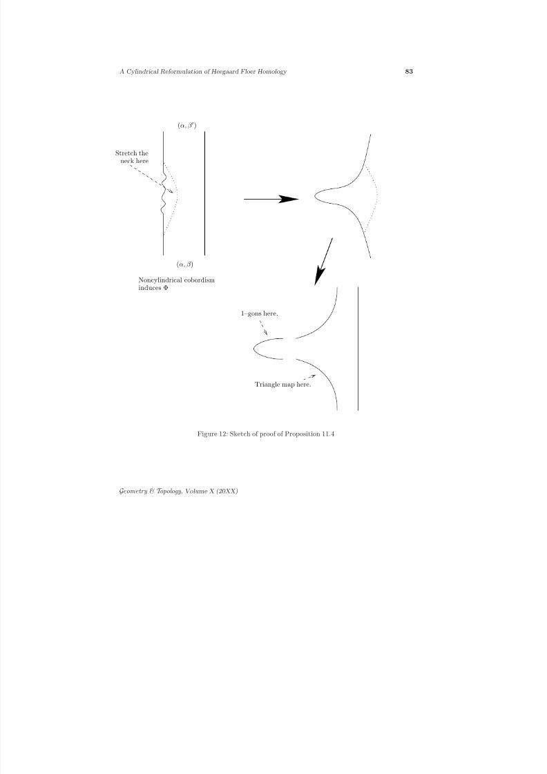
8/3/2019 Robert Lipshitz- A Cylindrical Reformulation of Heegaard Floer Homology
http://slidepdf.com/reader/full/robert-lipshitz-a-cylindrical-reformulation-of-heegaard-floer-homology 83/135
A Cylindrical Reformulation of Heegaard Floer Homology 83
1–gons here.
Noncylindrical cobordisminduces Φ
Stretch theneck here
Triangle map here.
(α, β ′)
(α, β )
Figure 12: Sketch of proof of Proposition 11.4
Geometry & T opology , Volume X (20XX)
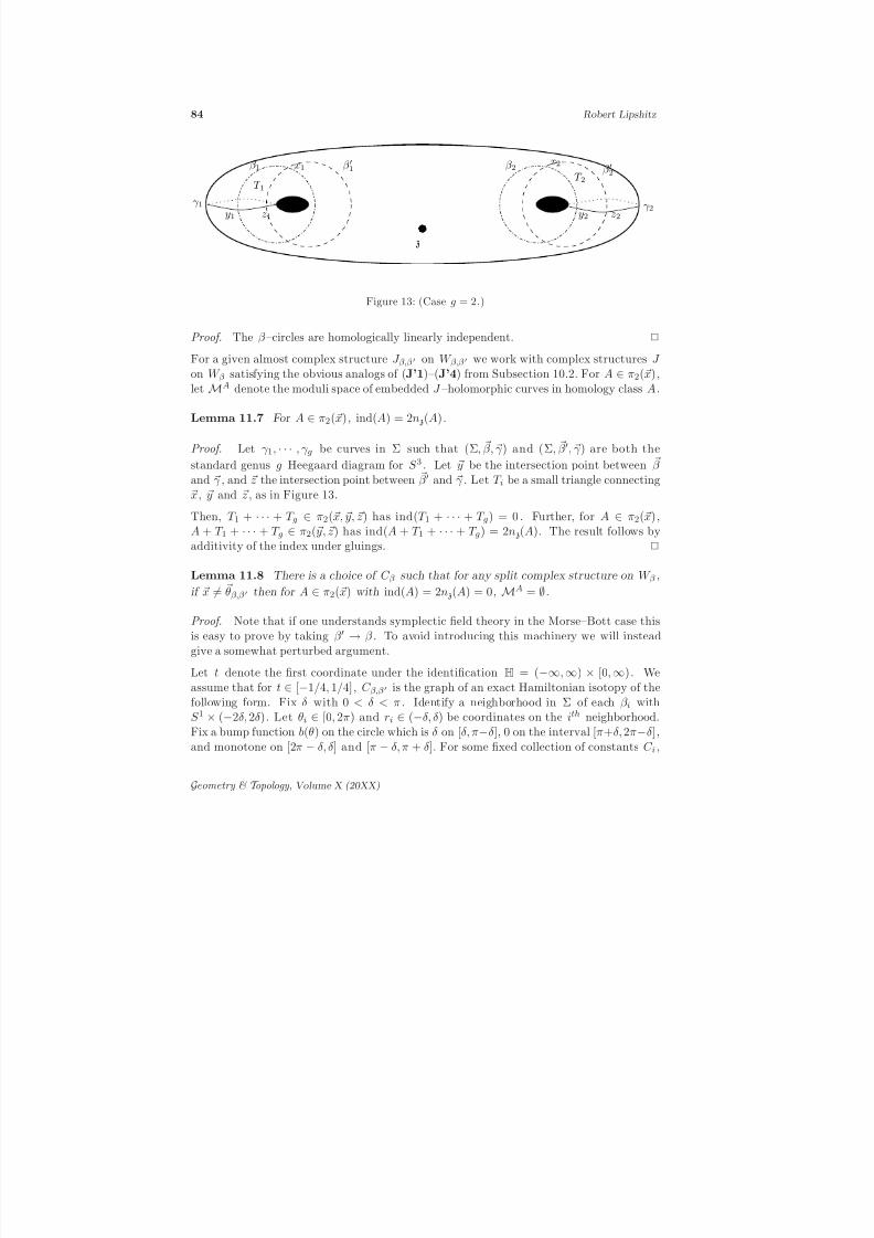
8/3/2019 Robert Lipshitz- A Cylindrical Reformulation of Heegaard Floer Homology
http://slidepdf.com/reader/full/robert-lipshitz-a-cylindrical-reformulation-of-heegaard-floer-homology 84/135
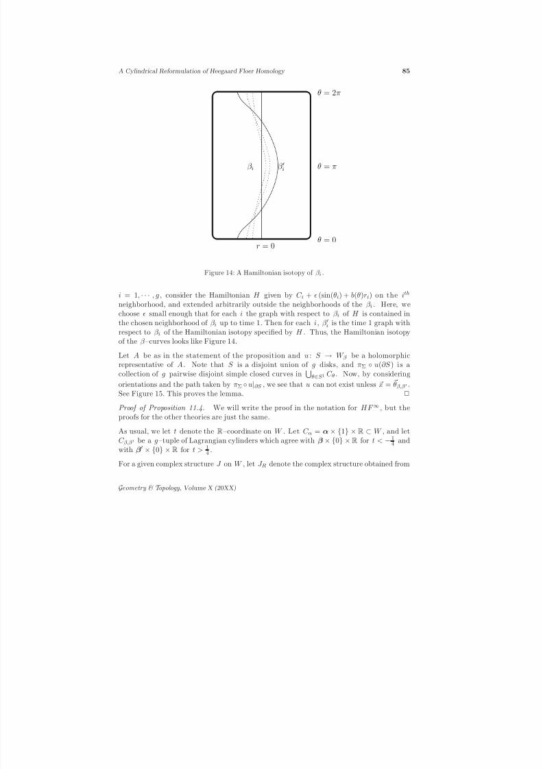
8/3/2019 Robert Lipshitz- A Cylindrical Reformulation of Heegaard Floer Homology
http://slidepdf.com/reader/full/robert-lipshitz-a-cylindrical-reformulation-of-heegaard-floer-homology 85/135
A Cylindrical Reformulation of Heegaard Floer Homology 85
β ′i
θ = 0
θ = 2π
θ = π
r = 0
β i
Figure 14: A Hamiltonian isotopy of β i .
i = 1, · · · , g , consider the Hamiltonian H given by C i + ǫ (sin(θi) + b(θ)ri) on the ith
neighborhood, and extended arbitrarily outside the neighborhoods of the β i . Here, we
choose ǫ small enough that for each i the graph with respect to β i of H is contained inthe chosen neighborhood of β i up to time 1. Then for each i, β ′i is the time 1 graph withrespect to β i of the Hamiltonian isotopy specified by H . Thus, the Hamiltonian isotopyof the β –curves looks like Figure 14.
Let A be as in the statement of the proposition and u : S → W β be a holomorphicrepresentative of A. Note that S is a disjoint union of g disks, and πΣ u(∂S ) is acollection of g pairwise disjoint simple closed curves in
θ∈S 1 C θ . Now, by considering
orientations and the path taken by πΣ u|∂S , we see that u can not exist unless x = θβ,β ′ .See Figure 15. This proves the lemma. 2
Proof of Proposition 11.4. We will write the proof in the notation for HF ∞ , but the
proofs for the other theories are just the same.
As usual, we let t denote the R–coordinate on W . Let C α = α × 1 × R ⊂ W , and letC β,β ′ be a g –tuple of Lagrangian cylinders which agree with β × 0 ×R for t < −1
4 andwith β′ × 0 × R for t > 1
4 .
For a given complex structure J on W , let J R denote the complex structure obtained from
Geometry & T opology , Volume X (20XX)
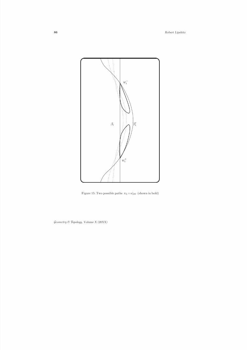
8/3/2019 Robert Lipshitz- A Cylindrical Reformulation of Heegaard Floer Homology
http://slidepdf.com/reader/full/robert-lipshitz-a-cylindrical-reformulation-of-heegaard-floer-homology 86/135
8/3/2019 Robert Lipshitz- A Cylindrical Reformulation of Heegaard Floer Homology
http://slidepdf.com/reader/full/robert-lipshitz-a-cylindrical-reformulation-of-heegaard-floer-homology 87/135
8/3/2019 Robert Lipshitz- A Cylindrical Reformulation of Heegaard Floer Homology
http://slidepdf.com/reader/full/robert-lipshitz-a-cylindrical-reformulation-of-heegaard-floer-homology 88/135
88 Robert Lipshitz
Proof. (Compare the proof of [21, Lemma 9.6].)
The following diagram commutes:
H 2(X α,β,βH ,β′ , ∂X α,β,βH,β′) o o ∼=
P.D. / / H 2(X α,β,βH,β′) o o ∼= / / ker
H 1(α) ⊕ H 1(β)⊕
H 1(βH ) ⊕ H 1(β′)
→ H 1(Σ)
H 1(∂X α,β,βH,β′)
O O
o o ∼=
P.D. / / H 2(∂X α,β,βH,β′)
O O
o o ∼= / /
ker(H 1(α) ⊕ H 1(β) → H 1(Σ))⊕
ker
H 1(β) ⊕ H 1(βH ) → H 1(Σ)
⊕
kerH 1(βH
) ⊕ H 1(β′
) → H 1(Σ)⊕
ker
H 1(β′) ⊕ H 1(α) → H 1(Σ)
O O O O
It is clear that the right hand vertical map is surjective. So, from the long exact se-quence of the pair (X α,β,β H,β ′ , ∂X α,β,β H ,β ′), the map H 2(X α,β,β H ,β ′) → H 1(∂X α,β,β H ,β ′)
∼=H 2(∂X α,β,β H ,β ′) is injective. But the image of δH 1(Y β,β ′) or δH 1(Y α,β H ) in the lattergroup is obviously 0. 2
Corollary 11.10
F α,β H ,β ′
F α,β,β H(· ⊗ θβ,β H) ⊗ θβ H,β ′
= F α,β,β ′
· ⊗ F β,β H ,β ′(θβ,β H ⊗ θβ H,β ′)
.
Similar statements hold for F ∞ , F + and F − with [θ, 0] (appropriately subscripted) in place of θ . (Compare [21, Lemma 9.6].)
Proof. From the previous lemma, the δH 1(Y β,β ′) + δH 1(Y α,β H)–orbit of SpinC–structureswhich restrict to s has just one element. Further, strong admissibility for the quadruple isequivalent to strong admissibility of the six Heegaard diagrams (Σ, α, β, z), · · · , (Σ, β H , β ′, z),which in turn follows from admissibility for (Σ, α, β, z). So, the result follows from Propo-sition 10.29. 2
Lemma 11.11 Let oα,β be a coherent orientation system for (Σ, α, β, z). Then there is a
coherent orientation system for the Heegaard quadruple–diagram (Σ, α, β, γ, δ, z) extending
oα,β and the orientation systems constructed in Proposition 11.3.
(In fact, it is not hard to see that the coherent orientation system for the Heegaardquadruple–diagram is essentially unique (compare Proposition 8.3).)
Proof. The orientation systems oα,β and oβ,β H extend to orientation systems oα,β,β H
and oα,β H by Lemma 10.10. For β ′ close to β , oα,β induces oα,β ′ , which extends to an
Geometry & T opology , Volume X (20XX)
8/3/2019 Robert Lipshitz- A Cylindrical Reformulation of Heegaard Floer Homology
http://slidepdf.com/reader/full/robert-lipshitz-a-cylindrical-reformulation-of-heegaard-floer-homology 89/135
A Cylindrical Reformulation of Heegaard Floer Homology 89
orientation system oα,β ′,β H . It is clear that we can perform the extensions so that the
induced orientations oβ ′,β H and oβ,β H are consistent with oβ,β H ,β ′ . The result follows. 2
Lemma 11.12 The map F ∞α,β,β H
(· ⊗ [θβ,β H , 0]) commutes with the actions of U and
H 1(Y α,β )/Tors . Similar statements hold for F + , F − and F .
Proof. The fact that F α,β,β H(· ⊗ [ θβ,β H , 0]) commutes with the U –action is obvious. Wecheck that it commutes with the H 1/Tors–action.
Fix a homology class ζ ∈ H 1(Y ). Choose a knot K → Σ representing ζ and meeting α
transversely. Let M1 denote the space of Riemann surfaces with 2g boundary punctures(as usual) and one additional marked point p on the boundary. We give yet another
definition of the map Aζ for a given (Σ, α, β, z). Given a homology class B ∈ π2(x, y), letMB
K denote the moduli space consisting of holomorphic maps from surfaces S ∈ M1 to
W α,β in the homology class B mapping p to K × 1 ×R, and MBK = MB
K /R. (Note thatthis definition is slightly different in form from the one we used to prove Proposition 8.6and Lemma 9.6. This definition is convenient here, but either would work.)
Now, for A ∈ π2(x, y, z), let MAK denote the space of holomorphic maps from surfaces
S ∈ M1 to W α,β,β H in the homology class A mapping p to K × e1 . (Recall that e1 is theedge of the triangle T corresponding to the α–circles.) Define a map H : CF ∞(Y α,β ) ⊗CF ∞(Y β,β H) → CF ∞(Y α,β H ) by
H ([x, i] ⊗ [y, j]) =
z A∈π2( x, y,z)ind(A)=0
#
MA
K [z, i + j − nz(A)].
For A ∈ π2(x, y, z), ind(A) = 1, consider the space MAK . This is a one–dimensional man-
ifold the ends of which are height two holomorphic buildings with an index 0 holomorphiccurve in W α,β,β H and an index 1 holomorphic curve (defined up to translation) in one of W α,β , W β,β H or W α,β H . For each of these buildings, either
(1) p is mapped to W α,β,β H or
(2) p is mapped to W α,β or
(3) p is mapped to W α,β H .
Summing the number of ends over the different choices of A with nz(A) = k we obtain, ineach case respectively,
(1) the coefficient of [z, i + j − k] in (∂ H + H ∂ )([x, i], [y, j])
(2) the coefficient of [z, i + j − k] in f ∞α,β,β H
(Aζ ([x, i]), [y, j]) or
(3) the coefficient of [z, i + j − k] in Aζ (f ∞α,β,β H([x, i], [y, j])).
Geometry & T opology , Volume X (20XX)
8/3/2019 Robert Lipshitz- A Cylindrical Reformulation of Heegaard Floer Homology
http://slidepdf.com/reader/full/robert-lipshitz-a-cylindrical-reformulation-of-heegaard-floer-homology 90/135
8/3/2019 Robert Lipshitz- A Cylindrical Reformulation of Heegaard Floer Homology
http://slidepdf.com/reader/full/robert-lipshitz-a-cylindrical-reformulation-of-heegaard-floer-homology 91/135
A Cylindrical Reformulation of Heegaard Floer Homology 91
the moduli spaces of curves we consider, correctly defined, are naturally identified with the
moduli spaces for (Σ, α, β, z). A gluing result then shows that the moduli spaces in thelimit can be identified with those of large neck length. Since the Floer homologies areindependent of complex structure, the invariance under stabilization will then follow.
Actually, although everything we say in this section is correct, it is somewhat dishonest:we leave most of the work for Proposition A.3 in the appendix. In particular, becauseof transversality issues, to prove the necessary gluing result we seem to need to work ina more harshly p erturbed setting than we use in this section. Much of the work of thepresent section is redone in the proof of Proposition A.3 in the more general context. Forexample, we prove there a stronger version of the compactness result Proposition 12.4.
I have chosen to write this section in this slightly dishonest way for two reasons. Firstly,
perhaps someone else will see a simpler way to correct the dishonesty (see the discussion atthe beginning of the proof of Proposition 12.4). Secondly, as written this section is quiteexplicit, so one can actually see what is going on in the stabilization proof.
Returning to mathematics, observe that from the formula for the index in Section 4 we knowthat for a homology class A ∈ πΣ
2 (x, y) corresponding to A′ ∈ πΣ′2 (x, y), ind(A) = ind(A′).
Since we only consider curves with index 1 when computing Floer homologies, we shallgenerally restrict to curves of index 1. This allows us to keep our definitions simpler andour theorems true.
We make precise what we mean by stretching the neck. Fix complex structures jΣ on Σand jT on T . Fix a point z0 ∈ T \ (αg+1 ∪ β g+1). Choose small disks DΣ ⊃ D′
Σ ∋ z and
DT ⊃ D′T ∋ z0 so that DΣ \ D
′Σ is conformally identified with S
1
× [−1, 0] and DT \ D′T is
conformally identified with S 1 × [0, 1]. Here, ∂D′Σ is identified with S 1 × −1 and ∂D ′
T
is identified with S 1 × 1. (The complex structure on a cylinder S 1 × [a, b] is given byidentifying the cylinder with er+iθ ∈ C|a ≤ r ≤ b under the identification (θ, t) → et+iθ .)
Let jR be the complex structure on
Σ′R = (Σ \ D′
Σ)
DΣ\D′Σ∼S
1×[−R−1,−R]
S 1 × [−R − 1, R + 1]
S 1×[R,R+1]∼∂DT
(T \ DT )
induced by the complex structures on Σ, T and S 1 × [−R − 1, R + 1], and ωR the areaform. We refer to S 1 × [−R − 1, R + 1] as the neck, and denote it N R . Notice that in the
limit R → ∞ , jR degenerates to the complex structure j∞ = jΣ ∨ jT on Σ ∨ T .Fix a complex structure J on W ′0 = Σ′
0 × [0, 1] ×R satisfying (J1)–(J5), which is split (i.e., j0 × jD) near N 0 . Let J R be the complex structure on W ′R = Σ′
R × [0, 1] ×R which agreeswith J outside N R× [0, 1]×R and with jR× jD on N R× [0, 1]×R. Note that J R convergesto a complex structure J ∞ on W ′∞ = (Σ ∨ T ) × [0, 1] ×R. The space W = Σ × [0, 1] × R
lies inside W ′∞ in an obvious way. We choose J so that
Geometry & T opology , Volume X (20XX)
8/3/2019 Robert Lipshitz- A Cylindrical Reformulation of Heegaard Floer Homology
http://slidepdf.com/reader/full/robert-lipshitz-a-cylindrical-reformulation-of-heegaard-floer-homology 92/135
8/3/2019 Robert Lipshitz- A Cylindrical Reformulation of Heegaard Floer Homology
http://slidepdf.com/reader/full/robert-lipshitz-a-cylindrical-reformulation-of-heegaard-floer-homology 93/135
A Cylindrical Reformulation of Heegaard Floer Homology 93
Proof. The restriction of πD v1 to the components on which it is nonconstant is a 1–fold
covering of the disk. Hence, it must be a disk itself. It follows easily that the restrictionof πT v1 to this component must be constant. Since the condition on z guaranteesthat the set (πD v1)
(πT v1)−1( z0)
consists of nz([u1]) = nz([v1]) distinct points, each
component on which πDv1 is constant must be a copy of T 2 , and the restriction of πT v1
to each component must be a diffeomorphism. 2
Corollary 12.3 The moduli space of holomorphic twin towers in a given homology class A ∈ πΣ
2 ( x, y) with ind(A) = 1 is naturally identified with MAW .
Here,
MA
W denotes the moduli space of holomorphic curves in the homology class A inW .
We now need to identify the space of holomorphic twin towers with MAW ′R
for R large
enough. As usual, doing so requires two steps: compactness and gluing. To avoid work wetorture the compactness argument slightly.
Proposition 12.4 Fix a sequence uR of J R–holomorphic curves in W ′ with index 1. Then for z chosen generically, there is a subsequence of uR which converges to a holomorphic twin tower (of height one).
Proof. The proof is in three stages. First we use the fact that πD uR is holomorphic toextract the vertical level structure and conformal structure on the limit surface. Then we
cut Σ into two overlapping regions, and view the uR as maps into each of the two regionswith Lagrangian boundary conditions. This allows us to extract a convergent subsequenceof maps to W ′ .
By classical symplectic field theory ([2, Theorem 10.1]), we can replace uR by a subsequenceso that πD uR converges to a holomorphic building, which we denote πD u∞ (althoughu∞ does not yet make sense on its own). We can also assume that for all R the source of uR is some fixed topological manifold S . Let S ∞ denote the source of πD u∞ .
Let C = S 1 × 0 ⊂ Σ′R denote the curve in Σ′ along which we are splitting. For
convenience, let us say that Σ “lies to the left of C ” while T “lies to the right of C .” LetC Σ = S 1 × −R − 1 ⊂ Σ′
R . Let C T = S 1 × −R − 1 + ρ ⊂ Σ′R for some ρ < R +1. Then,
C Σ and C T lie to the left of C , and C T lies to the right of C Σ . Note that the complexstructures J R are split to the right of C Σ . We will choose ρ large enough that C T liesclose to C in a sense we will specify soon. Let RC Σ denote the region to the right of C Σand LC T denote the region to the left of C T . See Figure 16.
Let C k, Aℓ denote the collection of disjoint circles and arcs in S along which the complexstructure degenerates.
Geometry & T opology , Volume X (20XX)

8/3/2019 Robert Lipshitz- A Cylindrical Reformulation of Heegaard Floer Homology
http://slidepdf.com/reader/full/robert-lipshitz-a-cylindrical-reformulation-of-heegaard-floer-homology 94/135
94 Robert Lipshitz
RC ΣLC T
C T
C ΣC
Figure 16: Interpolating Lagrangian cylinders
Let S RC Σ,R = (πΣ uR)−1(RC Σ). Since J R is split over RC Σ ,
πΣ uR : (S RC Σ,R, ∂S RC Σ,R) →
RC Σ, C Σ ∪ αg+1 ∪ βg+1
is a holomorphic map. So, again by classical symplectic field theory ([2, Theorem 10.3]),taking a further subsequence we can assume that πΣuR|S RCΣ,R converges to a holomorphicbuilding. We denote this building by πΣ u∞ , with the understanding that it is, so far,
only defined over S RC Σ,∞ .
It now makes sense to talk about the circles in C k which correspond to the degenerationalong C – i.e. the level splitting of πΣ uR . Let p j denote the corresponding points inS ∞ .
Since the arcs and circles C k, Aℓ are disjoint, we can choose C T close enough to C (i.e.,ρ large enough) that (πΣ u)−1(C T ) is disjoint from all the C k and Aℓ . We can also chooseρ so that πΣ u∞ is transverse to C T . We do so choose it. It follows that for R largeenough πΣ uR is transverse to C T .
Now, observe that each curve in (πD uR)(πΣ uR)−1(C T ) converges in the C ∞–topology
as R → ∞ . Let BR = (πD
uR)(πΣ uR)
−1
(C T ). Let B∞ = limR→∞ BR .Let LC T denote the portion of Σ′ to the left of C T . View [0, 1] as lying inside S 1 =[0, 2]/(0 ∼ 2), say. We can, thus, consider πD uR as a map to S 1 ×R. Consider the sym-plectic 4–manifold with boundary LC T × S 1 ×R, given the obvious (split) symplectic form.For each R, C T × BR is an immersed Lagrangian submanifold, and these submanifoldsC ∞ converge to C T × B∞ .
Geometry & T opology , Volume X (20XX)
8/3/2019 Robert Lipshitz- A Cylindrical Reformulation of Heegaard Floer Homology
http://slidepdf.com/reader/full/robert-lipshitz-a-cylindrical-reformulation-of-heegaard-floer-homology 95/135
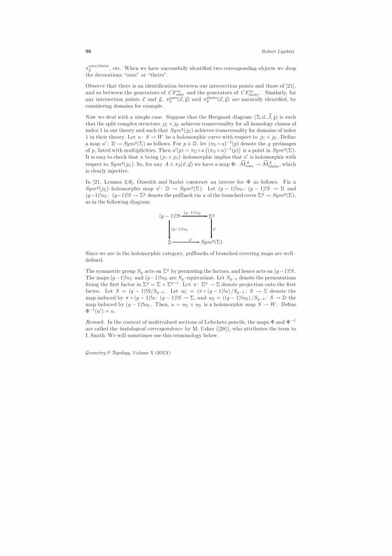
8/3/2019 Robert Lipshitz- A Cylindrical Reformulation of Heegaard Floer Homology
http://slidepdf.com/reader/full/robert-lipshitz-a-cylindrical-reformulation-of-heegaard-floer-homology 96/135
96 Robert Lipshitz
πours/theirs2 , etc. When we have successfully identified two corresponding objects we drop
the decorations “ours” or “theirs”.
Observe that there is an identification between our intersection points and those of [21],and so between the generators of CF ∞ours and the generators of CF ∞theirs . Similarly, forany intersection points x and y , πours
2 (x, y) and πtheirs2 (x, y) are naturally identified, by
considering domains for example.
Now we deal with a simple case. Suppose that the Heegaard diagram (Σ, α, β, z) is suchthat the split complex structure jΣ × jD achieves transversality for all homology classes of index 1 in our theory and such that Symg( jΣ) achieves transversality for domains of index1 in their theory. Let u : S → W be a holomorphic curve with respect to jΣ × jD . Definea map u′ : D → Symg(Σ) as follows. For p ∈ D, let (πD u)−1( p) denote the g preimages
of p, listed with multiplicities. Then u′( p) = πΣ u (πD u)−1( p) is a point in Symg(Σ).It is easy to check that u being ( jΣ × jD)–holomorphic implies that u′ is holomorphic with
respect to Symg( jΣ). So, for any A ∈ π2(x, y) we have a map Φ: MAours → MA
theirs , whichis clearly injective.
In [21, Lemma 3.6], Ozsvath and Szabo construct an inverse for Φ as follows. Fix aSymg( jΣ)–holomorphic map u′ : D → Symg(Σ). Let (g − 1)!uD : (g − 1)!S → D and(g−1)!uΣ : (g−1)!S → Σg denote the pullback via u of the branched cover Σg → Symg(Σ),as in the following diagram:
(g − 1)!S (g−1)!uΣ / /
(g−1)!uD
Σg
p
D
u′ / / Symg(Σ)
Since we are in the holomorphic category, pullbacks of branched covering maps are well–defined.
The symmetric group S g acts on Σg by permuting the factors, and hence acts on (g − 1)!S .The maps (g −1)!uΣ and (g −1)!uD are S g–equivariant. Let S g−1 denote the permutationsfixing the first factor in Σg = Σ × Σg−1 . Let π : Σg → Σ denote projection onto the firstfactor. Let S = (g − 1)!S/S g−1 . Let uΣ = (π (g − 1)!u) /S g−1 : S → Σ denote themap induced by π (g − 1)!u : (g − 1)!S → Σ, and uD = ((g − 1)!uD) /S
g−1: S → D the
map induced by (g − 1)!uD . Then, u = uΣ × uD is a holomorphic map S → W . DefineΦ−1(u′) = u.
Remark. In the context of multivalued sections of Lefschetz pencils, the maps Φ and Φ−1
are called the tautological correspondence by M. Usher ([28]), who attributes the term toI. Smith. We will sometimes use this terminology below.
Geometry & T opology , Volume X (20XX)
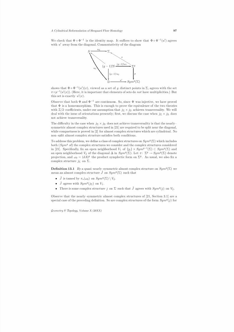
8/3/2019 Robert Lipshitz- A Cylindrical Reformulation of Heegaard Floer Homology
http://slidepdf.com/reader/full/robert-lipshitz-a-cylindrical-reformulation-of-heegaard-floer-homology 97/135
A Cylindrical Reformulation of Heegaard Floer Homology 97
We check that Φ Φ−1 is the identity map. It suffices to show that Φ Φ−1(u′) agrees
with u′ away from the diagonal. Commutativity of the diagram
S uΣ / /
uD
Σ
(g − 1)!S (g−1)!uΣ / /
(g−1)!uD
c c G G G G G G G G G G G G G
Σg
p
π
e e L L L L L L L L L L L L L L L L L
Du′ / / Symg(Σ)
shows that Φ Φ
−1
(u
′
)(x), viewed as a set of g distinct points in Σ, agrees with the setπ p−1(u′(x)). (Here, it is important that elements of sets do not have multiplicities.) Butthis set is exactly u′(x).
Observe that both Φ and Φ−1 are continuous. So, since Φ was injective, we have provedthat Φ is a homeomorphism. This is enough to prove the equivalence of the two theorieswith Z/2–coefficients, under our assumption that jΣ × jD achieves transversality. We willdeal with the issue of orientations presently; first, we discuss the case when jΣ × jD doesnot achieve transversality.
The difficulty in the case when jΣ × jD does not achieve transversality is that the nearly–symmetric almost complex structures used in [21] are required to be split near the diagonal,while compactness is proved in [2] for almost complex structures which are cylindrical. No
non–split almost complex structure satisfies both conditions.
To address this problem, we define a class of complex structures on Symg(Σ) which includesboth (Symg of) the complex structures we consider and the complex structures consideredin [21]. Specifically, fix an open neighborhood V 1 of zi × Symg−1(Σ) ⊂ Symg(Σ) andan open neighborhood V 2 of the diagonal ∆ in Symg(Σ). Let π : Σg → Symg(Σ) denoteprojection, and ω0 = (dA)g the product symplectic form on Σg . As usual, we also fix acomplex structure jΣ on Σ.
Definition 13.1 By a quasi–nearly–symmetric almost complex structure on Symg(Σ) we mean an almost complex structure J on Symg(Σ) such that
•˜
J is tamed by π∗(ω0) on Symg
(Σ) \ V 2 .• J agrees with Symg( jΣ) on V 1 .
• There is some complex structure j on Σ such that J agrees with Symg( j) on V 2 .
Observe that the nearly–symmetric almost complex structures of [21, Section 3.1] are aspecial case of the preceding definition. So are complex structures of the form Symg( j) for
Geometry & T opology , Volume X (20XX)

8/3/2019 Robert Lipshitz- A Cylindrical Reformulation of Heegaard Floer Homology
http://slidepdf.com/reader/full/robert-lipshitz-a-cylindrical-reformulation-of-heegaard-floer-homology 98/135
98 Robert Lipshitz
any complex structure j on Σ which is tamed by dA and agrees with jΣ near the zi . So, a
path of nearly–symmetric almost complex structures is a path of quasi–nearly–symmetricalmost complex structures. Also, an almost complex structure J on W satisfying (J1)–J5)corresponds to a path J s of complex structures on Σ, which in turn specifies a path of quasi–nearly–symmetric almost complex structures on Symg(Σ), which we denote Symg(J s).
For a path J t of quasi–nearly–symmetric almost complex structures, let jt be the complexstructure on Σ such that J t agrees with Symg( jt) on V 2 .
Now, we prove the equivalence of our theory with that of [21] in three steps. First weshow that the compactness proof of [21] extends to J t–holomorphic curves in Symg(Σ),where J t is a path of quasi–nearly–symmetric almost complex structures. Then we observethat the class of paths of almost complex structures of the form Symg(J s) is sufficient to
achieve transversality for holomorphic disks in Sym
g
(Σ). Finally we show that our modulispaces of J s–holomorphic curves can be identified with the Ozsvath–Szabo moduli spacesof Symg(J s)–holomorphic curves.
After proving the following proposition, the first and third steps are essentially immediate.
Proposition 13.2 Fix a path J t of quasi–nearly–symmetric almost complex structures on Symg(Σ). Fix a holomorphic disk u′ : (D, ∂ D) → (Symg(Σ), T α ∪ T β ). Then there is a g!–fold branched covering uD : S → D and a map uΣ : S → Σg such that the following diagram commutes.
S uΣ / /
uD
Σg
p
D
u′ / / Symg(Σ)
.
The map uΣ is holomorphic with respect to the path of almost complex structures on Σg
induced by J t , in the obvious sense, and is S g–equivariant.
Proof. The idea of the proof is that even though the complex structure is allowed to varynear the diagonal, since it varies in the class of split structures, locally near the diagonal weare still in the integrable case. The model for this argument is used to prove the following
Lemma 13.3 Under the assumptions of Proposition 13.2, u′ intersects the diagonal ∆
in a discrete collection of points.
Proof. Suppose that u′ intersects the diagonal ∆ in a collection of points p j with limitpoint p. Throwing out some of the points we may assume all of the p j lie in the samestratum of ∆. For concreteness we will assume all of the p j lie in the top dimensionalstratum of ∆, but there is nothing special about this case.
Geometry & T opology , Volume X (20XX)
8/3/2019 Robert Lipshitz- A Cylindrical Reformulation of Heegaard Floer Homology
http://slidepdf.com/reader/full/robert-lipshitz-a-cylindrical-reformulation-of-heegaard-floer-homology 99/135
8/3/2019 Robert Lipshitz- A Cylindrical Reformulation of Heegaard Floer Homology
http://slidepdf.com/reader/full/robert-lipshitz-a-cylindrical-reformulation-of-heegaard-floer-homology 100/135
100 Robert Lipshitz
(2) The coherence conditions for the two theories agree. That is, there is an identification
of the determinant line bundles Lours and Ltheirs with respect to which any coherentorientation oours of Lours specifies a coherent orientation otheirs of Ltheirs .
To keep the exposition clean, we will assume that the complex structure is split near thediagonal. As noted earlier, this assumption is quite restrictive. It can be removed byusing, at appropriate times, a parametrized version of the Riemann mapping theorem toidentify a neighborhood of uΣ (branch points of uD) with a standard disk, as in the proof of Lemma 13.3. (Alternately, given a curve u, we can choose a family J ′s : T Σ → T Σof almost complex structures on Σ constant near Φ(u) ∩ ∆ and such that the (Σ, J ′s)are conformally isomorphic to the original family (Σ, J s), and then work with the family(Σ, J ′s).) We leave further details to the interested reader.
From now on, when we want to discuss both our and their theories at once, we will drop the“ours” or “theirs” from the notation, even if we have not yet identified the correspondingobjects.
Recall from Section 3 that the tangent space at u to Bours is R2g ⊕ L p,d1 (u∗TW,∂ ), wherethe R2g includes into Γ (u∗T W ) as Span
v±i
where the v±i are some fixed smooth
sections with v±i equal to ∂ ∂t in a small neighborhood of the ith positive or negative punc-
ture and zero outside a slightly larger neighborhood of that puncture and L p,d1 (u∗TW,∂ )denotes sections tangent to C α ∪ C β over ∂S . The tangent space at φ to Btheirs is just
L p,d1 (φ∗T Symg(Σ), ∂ ) of L p,d1 sections tangent to T α ∪ T β over ∂ D and we take as a modelfor D the strip [0, 1] × R.
There is the minor complication that we are working in R–invariant settings, so rigid curveshave ind = 1. For convenience, we introduce the operator P u,ours : R2g ⊕ L p,dk (u∗TW,∂ ) →R defined by P u,ours(v1, v2) = v2,∂/∂tL2 . (Here, ·, ·L2 denotes the L2 inner productinduced by some Riemannian metric on W and a canonical metric on the source S of u. Since L
p,dk is finer than L2 , the operator P u,ours is continuous.) Then we replace
the linearized ∂ –map D∂ ours by D∂ ours = D∂ ours ⊕ P ours . Similarly, for ∂ theirs , letP φ,theirs(v) = v,dφ(∂/∂t)L2 , where ∂/∂t generates the one–parameter group of automor-phisms of (D2, i, −i). Then, replace D∂ theirs with D∂ theirs = D∂ theirs ⊕ P theirs . We retainthe old meaning of ind, so the index of Du∂ ours/theirs is ind(u) − 1.
We tackle point (1) of the proposition first. We begin by recalling how the coherent orien-
tation specifies signs of curves. Let u be a curve (not necessarily holomorphic), ind(u) = 1,at which D∂ (or equivalently D∂ ) is surjective. We can view the coherent orientation o
as a nonvanishing section of L, defined up to multiplication by a positive scalar function.At u, there is also a canonically defined section
1 ⊗ 1∗ ∈ R⊗R∗ =
Λ0R
0
⊗
Λ0R
0∗
=
Λtop ker(Du∂ )
⊗
Λtopcoker(Du∂ )∗
= Lu.
Geometry & T opology , Volume X (20XX)
8/3/2019 Robert Lipshitz- A Cylindrical Reformulation of Heegaard Floer Homology
http://slidepdf.com/reader/full/robert-lipshitz-a-cylindrical-reformulation-of-heegaard-floer-homology 101/135
8/3/2019 Robert Lipshitz- A Cylindrical Reformulation of Heegaard Floer Homology
http://slidepdf.com/reader/full/robert-lipshitz-a-cylindrical-reformulation-of-heegaard-floer-homology 102/135
102 Robert Lipshitz
If we allow the complex structure on S to vary, then there is an additional term. The tan-
gent space to Teichmuller space at S is a finite–dimensional subspace of C ∞ (End(TS ,j)),where End(TS ,j) is the space of endomorphisms of T S anticommuting with j . The lin-earized ∂ –operator is then a restriction of the map
Du∂ : R2g ⊕ L p,d1 (u∗TW,∂ ) ⊕ C ∞ (End(TS ,j)) → L p,d(Λ0,1u∗T W )
defined by
Du∂ (ξ, Y )(v) =1
2
∇vξ + J ∇ j(v)ξ
−
1
2J (∇ξJ ) ∂ J (v)(u) +
1
2J du Y (v).
For maps φ : D → Symg(Σ) the formulas are the same except that the R2g–factors areabsent.
In the future, we will suppress the Lagrangians from the notation.
Fix ǫ > 0. Let Bours denote the collection of maps u in Bours for which
• uD is holomorphic,
• uD has only simple branch points p1, · · · , pℓ ,
• d( pi, p j) > 2ǫ for i = j , and
• uΣ has no branch points inside the Bǫ( pi), i = 1, · · · , ℓ.
Let Bours ⊂ Bours denote the space of maps u ∈ Bours for which uΣ is holomorphic over∪iu
−1D
(Bǫ( pi)). For ǫ sufficiently small, J generic, and ind(A) = 1, MAours ⊂ Bours . Note
that BAours is nonempty if and only if the intersection number ∆ · A of the diagonal in
Symg(Σ) with A ∈ H 2(Symg(Σ), T α ∪ T β ) is non–negative.
Let u : S → W be a map in Bours such that uD
has branch points p1, · · · , pℓ ∈ (0, 1) ×R
.Lemma 13.8 The tangent space to Bours at u is given by
T uBours = L p,dk ((πΣ u)∗T Σ, ∂ ) ⊕
⊕ℓi=1C
.
Proof. This is clear. A point in Bours is determined by a complex structure on S and amap from S to Σ. The complex structure is determined by the branch points p1, · · · , pℓ .2
An inclusion of T uBours into T uBours can be given as follows. The inclusion L p,d1 (u∗ΣT Σ, ∂ ) →
L p,d1 (u∗TW,∂ ) is obvious. We include Cℓ into the space of infinitesimal deformations of thealmost complex structure on the source. The Cℓ corresponds to moving the branch points
p1, · · · , pg in D. This, in turn, corresponds to deforming the almost complex structure jDon D. But any almost complex structure jD on D specifies an almost complex structure jS on S via js = (duD)−1 jD duD .
We choose a family of infinitesimal deformations parametrizing the Cℓ vanishing over thebranch points p1, · · · , pℓ , i.e., such that the almost complex structure remains fixed nearthe branch points.
Geometry & T opology , Volume X (20XX)

8/3/2019 Robert Lipshitz- A Cylindrical Reformulation of Heegaard Floer Homology
http://slidepdf.com/reader/full/robert-lipshitz-a-cylindrical-reformulation-of-heegaard-floer-homology 103/135
8/3/2019 Robert Lipshitz- A Cylindrical Reformulation of Heegaard Floer Homology
http://slidepdf.com/reader/full/robert-lipshitz-a-cylindrical-reformulation-of-heegaard-floer-homology 104/135
104 Robert Lipshitz
Since Φ(u)( pi) lies in the top–dimensional stratum of the diagonal, near Φ(u)( pi), Symg(Σ)
decomposes as Sym2
(Σ) × Σg−2 . The projection of v′ to T Σg−2 is given by the previousconstruction. This leaves us to define the projection v′1 of v′ to T Sym2(Σ).
Inside the Bǫ( pi), w is constant so the term J du Y in Du∂ is zero. Let U i bethe component of u−1
D(Bǫ( pi)) on which duD is singular. Identify U i and V i = uΣ(U i)
holomorphically with D. Then, T V i is identified with V i × C and u∗ΣT V i with U i × C.Further, v becomes a map U i → C, and the statement that Du∂v = 0 becomes thestatement that v : U i → C is holomorphic.
Now, Φ(u)(Bǫ( pi)) ⊂ Sym2(V i) ⊂ Sym2(C) ∼= C2 . So, Φ(u)∗T Sym2(Σ) is identified withBǫ( pi) ×C2 . The holomorphic map (uD, v) : U i → Bǫ( pi) ×C specifies a holomorphic mapv′1 : Bǫ( pi) → Sym2(C) ∼= C
2 by the same tautological correspondence used to define Φ.We view v′1 as a section of Φ(u)∗T Sym2(Σ). Observe that v′1 and hence v1 is tangent tothe diagonal.
It is easy to check that the two definitions of v′ agree over ∂Bǫ( pi).
Finally, by its definition, w corresponded to an infinitesimal deformation of jD .
Lemma 13.11 The pair (v′, w′) lies in the kernel of D∂ theirs .
Proof. This is direct from the definitions. Away from the diagonal, this follows fromthe fact that the complex structure and symplectic form on Symg(Σ) have the formSymg( jΣ) and Symg(ωΣ) respectively. Near the diagonal, on the Sym2(Σ) factor thekernel of D∂ theirs corresponds under the trivializations used above to holomorphic mapsBǫ( pi) → Sym2(C). The map v′ is holomorphic near the diagonal by the usual tautological
correspondence. 2
This proves that ker(D∂ ours) ⊂ ker(D∂ theirs). The reverse inclusion can be proved simi-larly, using the opposite direction Φ−1 of the tautological correspondence.
This proves part (1) of Proposition 13.7. It remains to check part (2), i.e,. that thecoherence conditions for the two theories agree. Before doing so, we prove another
Lemma 13.12 Fix A with ind(A) > 0 and A · ∆ ≥ 0. Let oAours and oAtheirs be sections of Lours and Ltheirs respectively. Let u1, u2 ∈ BA
ours with Dui∂ surjective for i = 1, 2.At ui we constructed an identification of Lours and Ltheirs . Suppose that with respect tothe identification of determinant liens at u1 , oAours(u1) is a positive multiple of oAtheirs(u1).
Then with respect to the identification of determinant lines at u2 , oAours(u2) is a positive
multiple of oAours(u2).
Proof. Choose a path ua in Bours from u1 to u2 . Choose also a family of subspaces H of L p,d
Λ0,1u∗aT Σ
such that the operator
Dua∂ : L p,d1 (u∗aT Σ, ∂ ) ⊕Cℓ ⊕ H → L p,d
Λ0,1u∗aT Σ
Geometry & T opology , Volume X (20XX)
8/3/2019 Robert Lipshitz- A Cylindrical Reformulation of Heegaard Floer Homology
http://slidepdf.com/reader/full/robert-lipshitz-a-cylindrical-reformulation-of-heegaard-floer-homology 105/135
A Cylindrical Reformulation of Heegaard Floer Homology 105
given by
Dua∂ (v,w ,x) = Dua∂ (v, w) + xis surjective for all a. Further, choose H so that all sections in H vanish near the branchpoints of uD . This is possible for a generic path ua .
Choose an orientation o(H ) of H , i.e., a section of ΛtopH . Then there is a canonicalisomorphism between the determinant lines of D∂ and D∂ .
Since the sections in H vanish near the branch points of uD , the space H specifies a sub-space H ′ of L p,d
Λ0,1Φ(ua)∗T Symg(Σ)
as follows: for x ∈ H and y ∈ T pD let y1, · · · , yg
be the preimages of y under uD . Then define
x(y) = x(y1), · · · , x(yg) ∈ T Φ(u)( p)Symg(Σ).
The vanishing of the sections in H near the branch points of uD also means that wehave an identification of ker(D∂ ours) and ker(D∂ theirs), defined in the same way as theidentification of ker(D∂ ours) and ker(D∂ theirs) above. Further, the following diagramcommutes:
Det(Dui∂ )
⊗o(H )∼=
∼= / / Det(DΦ(ui)∂ )
⊗o(H )∼=
Det(Dui∂ )∼= / / Det(DΦ(ui)∂ )
for i = 1, 2. But this implies the result. 2
Note that as a porism of Lemma 13.12 we also have an identification of determinant linesfor A with A · ∆ ≥ 0 but ind(A) ≤ 0.
Next we recall the definition of a coherent orientation. A coherent orientation consists of achoice of nonvanishing section o(A) of the determinant line bundle L over the configurationspace in the homotopy class A such that the following coherence condition is satisfied:
Let u1 ∈ BA1(x, y) and u2 ∈ BA2(y, z) be curves for which Dui∂ is surjective. In Ap-pendix A we construct a family of preglued curves u1ru2 ∈ BA1+A2( x, z). For r large,the kernel of Du1ru2∂ is identified with ker(Du1∂ ) ⊕ ker(Du2∂ ). So, oA1 ⊗ oA2 specifiesa section of LA1+A2 . The coherence condition is that oA1+A2 be a positive multiple of oA1 ⊗ oA2 . One must check that this condition is independent of u1 and u2 ; see for in-stance [3, Corollary 7]. (In the case that Dui∂ is not surjective, one stabilizes Dui∂ by afinite–dimensional oriented subspace of L p,d
Λ0,1u∗iT W
, as in the proof of Lemma 13.12.)
(From now on, when we write a sum A + B of homotopy classes of curves we implicitlyassume that the asymptotics of A at ∞ agree with those of B at −∞.)
Returning to our situation, fix a coherent orientation oours . By the previous lemma, thisspecifies an orientation oAtheirs for each A with ind(A) > 0 and A · ∆ ≥ 0. We will refer tothe collection of A with ind(A) > 0 and A · ∆ ≥ 0 as the positive cone and denote it C + .Note that [Σ] ∈ C + and for any A, A + N [Σ] ∈ C + for N sufficiently large.
Geometry & T opology , Volume X (20XX)

8/3/2019 Robert Lipshitz- A Cylindrical Reformulation of Heegaard Floer Homology
http://slidepdf.com/reader/full/robert-lipshitz-a-cylindrical-reformulation-of-heegaard-floer-homology 106/135
106 Robert Lipshitz
Lemma 13.13 The orientation otheirs is coherent over the positive cone. That is, for
A, B ∈ C + , with respect to the identification induced by gluing, oAtheirs ⊗ oBtheirs is a positive multiple of oA+B
theirs .
Proof. This follows from the commutativity of
LA1ours ⊗ LA2
ours / /
LA1theirs ⊗ LA2
theirs
LA1+A2ours
/ / LA1+A2theirs
up to positive scaling, which follows easily from the definitions of the various maps involved.2
Lemma 13.14 Any coherent orientation o over the positive cone can be extended uniquely to a coherent orientation over all configuration spaces.
Proof. Fix A, and N large enough that A+N [Σ] ∈ C + . Then the map LA⊗o[N Σ]
/ / LA+N [Σ]
and the orientation oA+N [Σ] specifies an orientation oA of LA . By the coherence of o overthe positive cone, the orientation oA is independent of N , and obviously agrees with o
over the positive cone. Commutativity of the following diagram, up to positive scaling,implies that o is coherent:
LA ⊗ LB⊗o[N 1Σ]⊗o[N 2Σ] / /
LA+N 1[Σ] ⊗ LB+N 2[Σ]
LA+B
⊗o[N 1Σ]⊗o[N 2Σ] / / LA+B+(N 1+N 2)[Σ].
(Here, the vertical maps are induced by gluing. This requires stabilizing the spaces involved,as discussed above.) 2
We have now proved part (2) of Proposition 13.7. This concludes the proof of Theorem 2.
14 Other Remarks
14.1 Elaborations of Heegaard Floer
The 4–dimensional approach that we have used suggests possible elaborations of the Floerhomology groups considered in this paper. For the first one, we will describe briefly theHF –case, the only case that I am confident works. Our new chain complex CF big is freelygenerated over Z[[t]] by the intersection points. The differential is ∂ big = ∂ 0+t∂ 1+t2∂ 2+· · ·.
Geometry & T opology , Volume X (20XX)

8/3/2019 Robert Lipshitz- A Cylindrical Reformulation of Heegaard Floer Homology
http://slidepdf.com/reader/full/robert-lipshitz-a-cylindrical-reformulation-of-heegaard-floer-homology 107/135
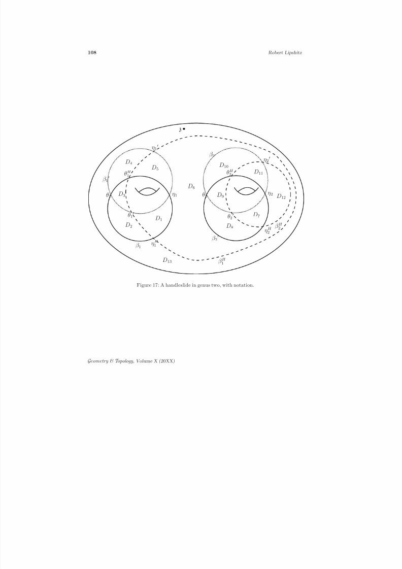
8/3/2019 Robert Lipshitz- A Cylindrical Reformulation of Heegaard Floer Homology
http://slidepdf.com/reader/full/robert-lipshitz-a-cylindrical-reformulation-of-heegaard-floer-homology 108/135
108 Robert Lipshitz
β 1
β 1′
β H 1
β H 2
β 2′
β 2
z
θ1 θ2η1 η2
ηH 2
ηH 1
θH 1θH 2
θ2′θ1
′
η1′
η2′
D1
D2
D3
D4D5
D6
D7
D8
D9
D10
D11
D12
D13
Figure 17: A handleslide in genus two, with notation.
Geometry & T opology , Volume X (20XX)
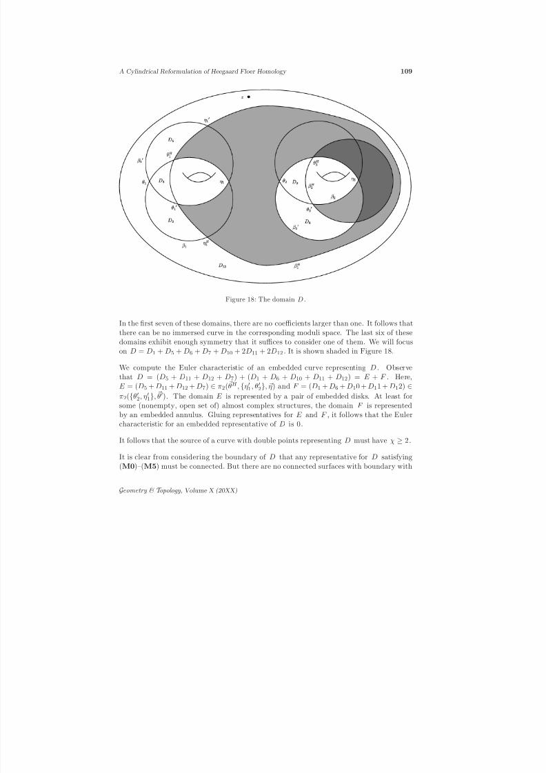
8/3/2019 Robert Lipshitz- A Cylindrical Reformulation of Heegaard Floer Homology
http://slidepdf.com/reader/full/robert-lipshitz-a-cylindrical-reformulation-of-heegaard-floer-homology 109/135
8/3/2019 Robert Lipshitz- A Cylindrical Reformulation of Heegaard Floer Homology
http://slidepdf.com/reader/full/robert-lipshitz-a-cylindrical-reformulation-of-heegaard-floer-homology 110/135
8/3/2019 Robert Lipshitz- A Cylindrical Reformulation of Heegaard Floer Homology
http://slidepdf.com/reader/full/robert-lipshitz-a-cylindrical-reformulation-of-heegaard-floer-homology 111/135
A Cylindrical Reformulation of Heegaard Floer Homology 111
intersection p oints. Define ∂ desc = ∂ 0 + 11!t∂ 1 + 1
2! t2∂ 2 + · · · where ∂ i counts holomorphic
curves u from Riemann surfaces S with i marked points p1, · · · , pi such that
• The homology class of u has index 2i + 1.
• For each i, u( pi) ∈ K × s0 × R.
• For each i, (πΣ u)′( pi) = 0.
Again, the proof that ∂ 2desc = 0 is standard. That the chain complex up to chain homotopyequivalence (over Z[[t]]) is an invariant of (Y, [K ]) is almost identical to the proof of invari-ance of the H 1/Tors–action on Heegaard Floer homology. There are no new computationsthat need to be done.
Of course, this is only one piece of a much bigger chain complex one could consider, where
one keeps track of higher branching of πΣ u and several different elements of H 1(Y ). Onecould also allow curves with branching of πΣ u at prescribed s0 and arbitrary point inΣ. Again, invariance of the bigger complex is free.
(One could also consider curves with prescribed branching of πD u, but taking s0 = 0 ourproof that bubbling is impossible forces higher differentials of this kind to be trivial.)
All of these deformed complexes should have roughly the same formal properties as Hee-gaard Floer homology. Unfortunately, even with this apparent wealth of additional infor-mation I have been unable to find nontrivial examples. That is, while there are exampleswhere higher differentials are nontrivial, I do not know examples which are not chain ho-motopy equivalent to complexes in which all higher differentials vanish. Hopefully this is
for lack of creativity or perseverance on my part.One might hope to construct further elaborations by pairing with cohomology classes of the space of maps S → W , but by Proposition 6.1 this space does not have interestingtopology. Finally, one might be able to obtain invariants by pulling back cohomologyclasses from the space of holomorphic maps to a disk. Doing so in a useful way, however,would require a better understanding of the cohomology of the moduli space of maps to adisk than I presently posses.
14.2 Relationship with Taubes’ program
We conclude with a few remarks about a likely relationship between Heegaard Floer homol-ogy as formulated in this paper and Taubes’ program to understand holomorphic curvesin 4–manifolds with singular symplectic forms.
First, a one paragraph sketch of Taubes’ idea. Any 4–manifold M with b+2 > 0 can
be endowed with a closed two–form ω which is nondegenerate in the complement of acollection of circles, and degenerates in a controlled way near the circles; see [26] for
Geometry & T opology , Volume X (20XX)
8/3/2019 Robert Lipshitz- A Cylindrical Reformulation of Heegaard Floer Homology
http://slidepdf.com/reader/full/robert-lipshitz-a-cylindrical-reformulation-of-heegaard-floer-homology 112/135
112 Robert Lipshitz
further information and references. The program is then to fix a complex structure J in
the complement of the singular circles, adjusted to ω , and obtain smooth invariants bystudying J –holomorphic curves of finite ω –energy in M .
The Floer homology associated to Taubes’ program would be structured as follows. Fora three–manifold Y , one chooses a closed 2–form ω on Y × R which is nondegenerate onthe complement of certain lines pi × R. One would then choose a translation invariantcomplex structure J on Y ×R adjusted to ω and study J –holomorphic curves with somespecified asymptotics at the singular lines and at Y × ±∞.
Fix a Morse function f on Y , and a metric on Y . Then, the form df ∧ dt + ⋆df is a closed2–form on Y ×R, which is nondegenerate on the complement of critical points of f ×R.(Here, ⋆ means the Hodge star on Y , not on Y × R.) One possible compatible complex
structure pairs dt with ∇f and is given by rotation by π/2 on ker(df ). We will call thisthe complex structure induced by f .
But this setting bears a close resemblance to (W, C α ∪ C β ). Assume f was self–indexing.Then, view Σ × [0, 1] as the slice f −1(3/2 − ǫ, 3/2 + ǫ) of Y . Then the complex structureinduced by f satisfies (J1)–(J5). Further, in the limit ǫ → 1/2, the boundary conditionswe impose become certain asymptotic conditions on the holomorphic curves at the singularlines. So, our setup fits quite nicely in Taubes’ picture.
A serious difficulty in studying holomorphic curves in Y ×R is understanding the asymp-totics at the singular lines. By studying only a middle slice of Y , Heegaard Floer homologyneatly avoids this issue. Still, it would be nice to be able to work in Y × R; for instance,
this would probably illuminate the proof of handleslide invariance.
A Gluing Lemmas
A.1 Statement of results
As seems conventional in the subject, we relegate the misery called “gluing lemmas” to theappendix.
In the following, by “symplectic manifold” we mean a symplectic manifold with cylindrical
ends, and by “complex structure” we mean a symmetric almost complex structure, asdefined in [2, Section 2]. We will always assume that Reeb orbits and chords correspondingto the almost complex structure and Lagrangian submanifolds in question are isolated, asthe Morse–Bott case requires extra work, and all Reeb chords in this paper are isolated.When we refer to a holomorphic curve we always mean ones with finite energy in the senseof [2, Section 6.1]. With these conventions, the gluing results used in this paper are
Geometry & T opology , Volume X (20XX)
8/3/2019 Robert Lipshitz- A Cylindrical Reformulation of Heegaard Floer Homology
http://slidepdf.com/reader/full/robert-lipshitz-a-cylindrical-reformulation-of-heegaard-floer-homology 113/135
A Cylindrical Reformulation of Heegaard Floer Homology 113
Proposition A.1 Let (M 1, M 2) be a chain of symplectic manifolds (cf. [6, Section 1.6])
with M 2 cylindrical. Let (u1, u2) be a height two holomorphic building in (M 1, M 2). As-sume that the complex structures on M 1 and M 2 are chosen so that the ∂ operator is trans-verse to the zero–section at u1 and u2 . Then there is a neighborhood of (u1, u2) in the space of (height one or two) holomorphic buildings diffeomorphic to Rind(u1)+ind(u2)−1 × (0, 1]. If M 1 is also cylindrical then the same statement holds with Rind(u1)+ind(u2)−1 replaced by Rind(u1)+ind(u2)−2 . Both statements remain true in the relative case.
Proposition A.2 Let (M 1, M 2) be a chain of symplectic manifolds (cf. [6, Section 1.6])obtained by splitting a symplectic manifold M along a co–oriented hypersurface H as in [2,Section 3.4]. Let (u1, u2) be a height two holomorphic building in (M 1, M 2). Assume that the complex structure on M is chosen so that the ∂ operator is transverse to the
zero–section at u1 and u2 . Let J R denote the complex structure on M obtained by inserting a neck of length R along H . Let MR denote the space of J R–holomorphic curves in M Then there is a neighborhood of (u1, u2) in the space
R MR diffeomorphic
to Rind(u1)+ind(u2) × (0, 1]. The statement remains true in the relative case.
Proposition A.3 Proposition A.2 remains true in the case of height one holomorphic twin towers studied in Section 12. That is, with notation as in Section 12, for ind(A) = 1,
we have # MAW ′R
= # MAW .
The special case of Proposition A.1 when M 1 is the symplectization of a contact manifoldfollows from work of Bourgeois ([1, Corollary 5.7]). His argument, however, extends without
essential changes to prove the more general results stated here. To demonstrate this, weimitate his argument to prove Proposition A.2 in the relative case. Proposition A.1 issimilar but marginally less complicated. After proving Proposition A.2 we discuss how theproof needs to be modified to prove Proposition A.3.
A.2 The splitting process
In this subsection we describe the process of splitting a symplectic manifold along a hy-persurface. More details can be found in [2, Section 3.4]. We describe the splitting process(tersely) here partly because the relative case is hardly discussed in [2] but mostly just to
fix notation.Let (M, ω) be a symplectic manifold, J a complex structure on M compatible with ω ,and H ⊂ M a co–oriented compact hypersurface. We also assume that we are given avector field R ∈ ker(ω|H ) on H so that the associated cylindrical structure on H × R issymmetric (see [2, p. 802]). Let α be the 1–form ω(J R, ·) on H . Then a neighborhoodof H is symplectomorphic to ((−ǫ, ǫ) × H, π∗H ω|H + d(tα)) so that J R is identified with
Geometry & T opology , Volume X (20XX)
8/3/2019 Robert Lipshitz- A Cylindrical Reformulation of Heegaard Floer Homology
http://slidepdf.com/reader/full/robert-lipshitz-a-cylindrical-reformulation-of-heegaard-floer-homology 114/135
8/3/2019 Robert Lipshitz- A Cylindrical Reformulation of Heegaard Floer Homology
http://slidepdf.com/reader/full/robert-lipshitz-a-cylindrical-reformulation-of-heegaard-floer-homology 115/135
A Cylindrical Reformulation of Heegaard Floer Homology 115
H . Note that E +0 = E −0 , where this identification respects the image of L and also the
Reeb field. We sometimes write E 0 for E ±0 .
For i = 0, · · · , N , let L ∩ E i = Li × I i . Let τ i denote the coordinate on I i , and Ri = J∂ τ i .Let Γo
i denote the space of closed orbits of Ri , Γci the space of Ri–chords, i.e., flows of Ri
starting and ending on Li . Let Γi = Γoi ∪ Γc
i .
We will assume throughout that the Γi are discrete.
Fix Reeb chords/orbits γ 0,1, · · · , γ 0,n0 ∈ Γ0 , γ +i,1, · · · , γ +i,n+i
∈ Γi (i = 1, · · · , N ), and
γ −i,1, · · · , γ i,n−i∈ Γi (i = 1, · · · , N ). For notational convenience, let γ +0,j = γ −0,j = γ 0,j .
Assume γ ±i,1, · · · , γ ±i,m±
i
∈ Γoi are closed Reeb orbits and γ i,m±
i +1, · · · , γ 0,n±i∈ Γc
i are Reeb
chords. For convenience and because it is the only case relevant to this paper we will
assume that all the γ 0,k and γ ±i,k are simple Reeb chords / orbits.
Fix smooth surfaces Σ± with boundary and labeled punctures
p±0,1, · · · , p±0,n0 , · · · , p±N,1, · · · , p±N,n±N
.
Let T ± be smooth families of conformal structures on Σ so that T ± surjects onto anopen set in the moduli space of Riemann surfaces. (That is, points in T ± are honestsurfaces with conformal structures and marked points, not equivalence classes of such.The map from T ± to moduli space need not be injective.) Choose T so that there aresmall neighborhoods of the punctures in Σ in which the conformal structure is constant.Fix p > 2, k ≥ 1. For convenience later, we will also fix S ±0 ∈ T ± .
For S ± ∈ T ± , let B±S ± = B p,d,±k denote the Banach manifold of W pk –maps (S ±, ∂S ±) →
(M ∞, L) converging to γ ±i,k at p±i,k (i = 0, · · · , N , k = 1, · · · , ni ) in W p,dk . That is:
Any R–chord or orbit γ has some period T γ defined by T γ = 12π
γ ω(∂ τ , ·) . If γ is a
Reeb orbit choose a tubular neighborhood N γ of γ invariant under the R–flow and adiffeomorphism φ from a neighborhood of S 1 × 0 in S 1 × R
2n−2 to N γ such that
(1) φ(S 1 × 0) = γ
(2) the pushforward under φ of T γ times the unit tangent vector to S 1 × 0 is R and
(3) φ∗ω|S 1× 0 = ω0|S 1× 0 , where ω0 denotes the standard symplectic form on R2n−2 .
If γ is a Reeb chord choose a tubular neighborhood N γ of γ invariant under the R–flowand a diffeomorphism φ from a neighborhood of [0, 1] × 0 in [0, 1] ×R2n−2 to N γ such that
(1) φ([0, 1] × 0) = γ
(2) the pushforward under φ of T γ times the unit tangent vector to [0, 1] × 0 is R and
(3) φ∗ω|[0,1]× 0 = ω0|[0,1]× 0 , where ω0 denotes the standard symplectic form on R2n−2 .
Geometry & T opology , Volume X (20XX)
8/3/2019 Robert Lipshitz- A Cylindrical Reformulation of Heegaard Floer Homology
http://slidepdf.com/reader/full/robert-lipshitz-a-cylindrical-reformulation-of-heegaard-floer-homology 116/135
116 Robert Lipshitz
(Compare [2, Lemma A.1], but note that our N γ is not the same as their N .) Let θγ
parametrize S 1 in the first case, or [0, 1] in the second case, by arc length. Let z =(x1, · · · , xn−1, y1, · · · , yn−1) be the standard coordinates on R2n−2 .
Via φ, θγ and z become coordinates on N γ .
For S ± ∈ T ± we fix a holomorphic identification of a neighborhood of each p±i,j with
[0, ∞)×S 1 if p±i,j is in the interior of S ± and with [0, ∞)× [−π, π] if p±i,j is in the boundary
of S ± . Let (t, s) denote the coordinates near p±i,j induced by this decomposition.
The statement that a map u± : S ± → M ∞ is asymptotic to γ ±i,j at p±i,j means that for
some τ ±i,j,0, θ±i,j,0 ∈ R, z u±(t, s) → 0 as t → ∞, τ u±(t, s) − σiT γ i,j t − σiτ ±i,j,0 → 0 as
t → ∞ and θ u±(t, s) − s − θ±i,j,0 → 0 as t → ∞. We say that the map u± is L p,dk
near p±i,j if z u(t, s), τ u(t, s) − σiT γ i,j t − σiτ i,j,0 and θ u(t, s) − s − θ±i,j,0 are all inL p,dk = f |f (t, s)ed|t|/p ∈ L pk. Note that if γ i,j is a Reeb chord then θ±i,j,0 = 0 while if γ i,jis a closed Reeb orbit then after replacing s with s − θ±i,j,0 we can assume that θ±i,j,0 = 0.
In the future we will assume that s has been chosen so that θ±i,j,0 = 0. Replacing some of the neighborhoods of the punctures with smaller ones if necessary we can assume that foreach i the constants τ ±i,j,0 are all the same, τ ±i,j,0 = τ i,0 .
The compactness result [2, Theorem 10.2] and asymptotic convergence result [2, Proposi-tion 6.2] imply that there exists a d > 0 such that any holomorphic curve of finite energy
with the specified asymptotics is in B p,dk . Fix such a d, and let B± = B p,d,±k .
Similarly, for any Riemannian vector bundle E over S ± we can consider the space of L p,d
k–
sections of E , L p,dk (E ). The complex structure J and symplectic form ω induce a metric
on M ∞ , so it makes sense to talk about the space L p,dk−1(Λ0,1T ∗S ± ⊗J u∗T M ∞) of L p,dk−1
(0, 1)–forms on S ± with values in T ∗M .
Now, the spaces B±S ±
fit together into a fiber bundle B± over T ± . In turn, the spaces
L p,dk−1(Λ0,1T ∗S ±⊗J u∗T M ∞) fit together into a vector bundle E ± over B± . The ∂ –operator
gives a section B± → E ± . We will assume that this ∂ map is transversal to the 0–section.We let M± denote the intersection of ∂ with the 0–section.
Recall that we fixed reference Riemann surfaces S ±0 ∈ T ± . As all Riemann surfaces in T ±
have fixed smooth source Σ± , there is an obvious projection map B± → B±S ±0
. Identify B±
with T × B±S ±0
.
Remark. While we have not yet chosen metrics or norms on the spaces under consideration,when we do, a figment of the details of our definition is that the identification of B± withT × B±
S ±0will not induce isometries. However, by choosing T small we can make the
induced maps arbitrarily close to isometries.
Geometry & T opology , Volume X (20XX)
8/3/2019 Robert Lipshitz- A Cylindrical Reformulation of Heegaard Floer Homology
http://slidepdf.com/reader/full/robert-lipshitz-a-cylindrical-reformulation-of-heegaard-floer-homology 117/135

8/3/2019 Robert Lipshitz- A Cylindrical Reformulation of Heegaard Floer Homology
http://slidepdf.com/reader/full/robert-lipshitz-a-cylindrical-reformulation-of-heegaard-floer-homology 118/135
118 Robert Lipshitz
each with Lagrangian submanifolds obtained from L, which we still denote L. The split
manifold M ∞ has two new ends E ±0 corresponding to H .
We have families T ± of complex curves and spaces B± of W p,dk maps of curves in T ± intoM ∞ , asymptotic to Reeb orbits γ 0,1 = γ +0,1 = γ −0,1, · · · , γ 0,m0 = γ +0,m0
= γ −0,m0and Reeb
chords γ 0,m0+1 = γ +0,m0+1 = γ −0,m0+1, · · · , γ 0,n0 = γ +0,n0 = γ −0,n0 in the ends E ±0 at punctures
p±0,j and various other fixed Reeb chords in the other ends. We have defined bundles E ±
over B± of which ∂ is a section, and M± to be the intersection of ∂ with the 0–sectionof E ± . The linearized ∂ –operator is denoted
D∂ : W ±u± ⊕ F ± ⊕ L p,dk
u∗±T M ∞, ∂
→ L p,dk−1
Λ0,1u∗±T M ∞
where F ± ∼= CP
N i=0m
±
i ⊕ RPN i=0(n
±
i −m±
i ) is generated by sections v±τ,i,j and v±θ,i,j which
agree with ∂/∂τ and ∂/∂θ respectively near the puncture p±i,j . When restricting to a fixed
source S ± those objects are replaced by B±S ± , E ±
S ± , M±S ± , ∂ S ± and D∂ S ± respectively.
To perform the gluing we will need cutoff functions. Fix a smooth function β : R → [0, 1]such that
β (t) = 0 if t ≤ 0β (t) = 1 if t ≥ 1
0 ≤ β (ℓ)(t) ≤ 2ℓ for all t ∈ R and ℓ ∈ N.
For R/2 > T γ ±0,i, define the cutoff function β i,R(t) = β
T γ±0,i
(t−1)
R/2−T γ±0,i
, so that
β i,R(t) = 0 for t ≤ 1
β i,R(t) = 1 for t ≥ R2T
0 ≤ β (ℓ)i,R(t) ≤
2T
R/2−T
ℓfor all t ∈ R and ℓ ∈ N.
Remark. For our proofs, the explicit bounds on the higher derivatives will not be important.All that will matter is that all derivatives of β i,R are uniformly bounded in R, and thatβ ′i,R → 0 as R → ∞ .
A.4 Gluing estimates
Choose elements u± : S ± → M ∞ in M± . Let ind± denote the index of D∂ at u± .Since we are assuming transversality, there is a neighborhood of u± in M± diffeomorphicto R
ind± . We want to show that there is a neighborhood of the two–story holomorphicbuilding (u−, u+) in M diffeomorphic to Rind
−
× Rind+ × (0, 1]. To do this, we will use
the
Geometry & T opology , Volume X (20XX)
8/3/2019 Robert Lipshitz- A Cylindrical Reformulation of Heegaard Floer Homology
http://slidepdf.com/reader/full/robert-lipshitz-a-cylindrical-reformulation-of-heegaard-floer-homology 119/135
A Cylindrical Reformulation of Heegaard Floer Homology 119
Lemma A.5 (Implicit Function Theorem) Let f : E → F be a smooth map of Banach
spaces with a Taylor expansion
f (ξ) = f (0) + Df (0)ξ + N (ξ).
Assume Df (0) has a finite–dimensional kernel and a right inverse Q satisfying
QN (ξ) − QN (η) ≤ C (ξ + η) ξ − η,
for some constant C . Assume also that Qf (0) ≤ 18C . Then for δ = 1/(4C ), f −1(0) ∩
Bδ(ξ) is a smooth manifold of dimension dim ker Df (0). In fact, there is a smooth functionπ : ker Df (0) ∩ Bδ(ξ) → Q(F ) such that f (ξ + φ(ξ)) = 0 and all zeroes of f in Bδ(ξ) have the form ξ + φ(ξ).
This result is [7, Proposition 24, page 25]. The proof is essentially the same as the finite–dimensional case. The result, which A. Floer refers to as Newton’s method, is called“Floer’s Picard Lemma” by some authors. In the literature, I have found at least fiveincorrect references to its location.
We will apply the implicit function theorem to ∂ : B → E . Recall that for u : S → M ,T uB = V ⊕ F ⊕ L p,dk (u∗T M , ∂ ) for some finite–dimensional space V ⊕ F . Choose a norm
on V ⊕ F arbitrarily; together with the L p,dk –norm this makes T B into a Banach space.
We give two necessary general results before turning to the estimates needed by the implicitfunction theorem.
Lemma A.6 At (u : S → M ) ∈ W
p,d
k the remainder N in the Taylor expansion∂ (u + ∆u) = ∂ (u) + D∂ (u)∆u + N (∆u) ∈ L
p,dk−1(Λ0,1T ∗S ⊗J u
∗T M ∞)
for the ∂ –operator satisfies
N (ξ) − N (η) ≤ C ′ (ξ + η) ξ − η (11)
for ξ , η in V ⊕ F ⊕ L p,dk (u∗T M , ∂ ) and some constant C (depending on uW p,dk−1
). (Here,
we identify a neighborhood of the map u with a neighborhood of the 0–section in V ⊕ F ⊕L p,dk (u∗T M , ∂ ).)
Proof. The argument is essentially the same as the one used by Floer to prove [8, Theorem
3a], and we omit it. Floer finds a relatively explicit formula ([8, Lemma 3.2]) for N (ξ),using charts, and simple bounds on the terms in the formula. There are several differencesbetween our setup and the setup of [8]. We claim the bound (11) for all L p,dk , while Floer
only states it for L p,d1 ; however, Floer in fact proves the result for all L p,dk . The holomorphiccurves in [8] all have source a strip, but this is again essentially irrelevant for his proof. Theextra finite–dimensional spaces cause no additional complications. Finally, the asymptotics
Geometry & T opology , Volume X (20XX)
8/3/2019 Robert Lipshitz- A Cylindrical Reformulation of Heegaard Floer Homology
http://slidepdf.com/reader/full/robert-lipshitz-a-cylindrical-reformulation-of-heegaard-floer-homology 120/135

8/3/2019 Robert Lipshitz- A Cylindrical Reformulation of Heegaard Floer Homology
http://slidepdf.com/reader/full/robert-lipshitz-a-cylindrical-reformulation-of-heegaard-floer-homology 121/135
A Cylindrical Reformulation of Heegaard Floer Homology 121
where η±i and U ±i decay exponentially in ti .
Choose R0 large enough that for R > R0 and i = 1, · · · , n0 ,
∓R±τ ±0,0T γ0,i
, s±i
lies in the
neighborhood of p±0,i on which the coordinates in use are defined. From now on we will
assume that R > R0 . Then τ ± u±
∓R±τ ±0,0T γ0,i
, s±i
= ±R. So, define S +RS − to be the
surface obtained by deleting
∓t±i >
R±τ ±0,0T γ0,i
from S ± and gluing the resulting surfaces
along the newly created boundary in the obvious way. We will refer to the image of theneighborhoods of the punctures p±0,i in S +RS − as the necks. Define coordinates (t0i , s0
i )on the necks by
s0i = s+
i , t0i = t+i + R+τ 0,0T γ0,i
for t+i ≥ − R+τ 0,0T γ0,i
s0i = s−i , t0i = t−i − R−τ 0,0
T γ0,ifor t−i ≤ R−τ 0,0
T γ0,i
.
We define the pre–glued map u+Ru− : S +RS − → M R to agree with u+ or u− outsidethe necks. Recall that M R has a neck [−R, R] × E 0 ; let τ R denote the [−R, R]–coordinateon the neck of M R , and πE 0 projection of the neck of M R onto E 0 . Then, on the ith neckof S +RS − , u+Ru− is defined by
τ R (u+Ru−)(s0i , t0i ) = T γ 0,it
0i + β (t0i − 1)η+
i (s0i , t0i )
πE 0 (u+Ru−)(s0i , t0i ) = expγ 0,i(si) β (t0i − 1)U +i (s0
i , t0i ) if t0i ≥ 1
τ R (u+Ru−)(s0i , t0i ) = T γ 0,it
0i
πE 0 (u+Ru−)(s0i , t0i ) = γ 0,i(si)
if −1 ≤ t0i ≤ 1
τ R (u+Ru−)(s0i , t0i ) = T γ 0,it
0i + β (−t0i − 1)η−i (s0
i , t0i )πE 0 (u+Ru−)(s0
i , t0i ) = expγ 0,i(si)
β (−t0i − 1)U −i (s0i , t0i )
if t0i ≤ −1
(Compare [1, page 54].) Note that since L ∩ E 0 is totally geodesic and U ±i |∂S ± is tangentto L ∩ E 0 , this formula makes perfectly good sense in the relative setting.
We extend the gluing construction to a neighborhood of (u+, u−) in B+ × B− . The details
of this extension are unimportant, but for completeness we give them anyway. Extend thecoordinates (t±i , s±i ) smoothly to holomorphic coordinates on surfaces in a neighborhood of (S +, S −). Let θ1, · · · , θm0 be in some interval around 0 ∈ S 1 = R/Z and r1, · · · , rn0 in R,R > R0 . Let θm0+1 = · · · = θn0 = 0. Then, for (u′+ : S ′+ → M ∞, u′− : S ′− → M ∞), define
S ′+r1,··· ,rn0 ,θ1,··· ,θm0S ′− by deleting the disks
∓t±i >
ri±τ 0,0T γ0,i
from S ′± and identifying
the newly created boundaries by s+i ↔ s−i + θi . Define coordinates (t0i , s0
i ) on the necks of
Geometry & T opology , Volume X (20XX)

8/3/2019 Robert Lipshitz- A Cylindrical Reformulation of Heegaard Floer Homology
http://slidepdf.com/reader/full/robert-lipshitz-a-cylindrical-reformulation-of-heegaard-floer-homology 122/135
122 Robert Lipshitz
the glued surfaces bys0i = s+
i − β (t0i )θi t0i = Rri
t+i +ri+τ 0,0T γ0,i
for t+i ≥ −ri+τ +0,0T γ0,i
s0i = s−i , t0i = t−i − R
ri
ri−τ −
0,0
T γ0,ifor t−i ≤
ri−τ −
0,0
T γ0,i
Then, define u′+r1,··· ,rn0 ,θ1,··· ,θm0u′− by the same formula used to define u+Ru− above.
Let T R denote the space of conformal structures given by the gluing construction justexplained. Note that T R projects onto an open neighborhood of S +RS − in moduli space.Let BR denote the space of W p,dk maps from surfaces in T R with the specified boundaryconditions and asymptotics. Note that the glued maps fill out a neighborhood of u+Ru−in BR .
Recall that we defined spaces W ±
u± =: W ± as the image under D∂ of V ± = T S ±T . Since
the conformal structures in T agree near the punctures, we can view V +⊕V − as a subspaceof Γ(Λ0,1T ∗(S +RS −)) and W + ⊕ W − as a subspace of (u+Ru−)∗T M R for any R.
Recall also that we defined spaces F ± = CPN
i=0m±
i ⊕ RP
i=0N (n±i −m±
i ) corresponding tothe span of a fixed collection of
N i=0 m±
i vector fields v±τ,i,j and v±θ,i,j given by ∂ ∂τ and
∂ ∂θ near the
N i=0 m±
i interior punctures and a fixed collection of N
i=0(n±i − m±i ) vector
fields v±τ,i,j given by ∂ ∂τ near the
N i=0(n±i − m±
i ) boundary punctures of u± . Let
F 0 = Spanvτ,0,j , vθ,0,j = C
PN i=1(m
+i m
−
i ) ⊕R
PN i=1(n
+i +n−i −m
+i −m
−
i )
be the sections corresponding to punctures which are not being glued.
The tangent space T T R is Cm0
⊕Rn0−m0
⊕V +
⊕V −
. (The C– and R–summands correspondto the gluing parameters θi and ri .) So, the tangent space to BR is
T u+Ru−BR = Cm0 ⊕ R
n0−m0 ⊕ V + ⊕ V − ⊕ F 0 ⊕ L p,dk ((u+Ru−)∗T M R, ∂ ) . (12)
The map V + ⊕ V − → W + ⊕ W − induced by D∂ is a surjective map of finite–dimensionalvector spaces, and independent of R. It therefore has a uniformly bounded right inverse.It therefore suffices to construct a uniformly bounded right inverse to the map
Cm0 ⊕R
n0−m0 ⊕ W + ⊕ W −⊕ F 0 ⊕ L p,dk ((u+Ru−)∗T M R, ∂ )
→L p,dk−1
Λ0,1(u+Ru−)∗T M R
given by
(vC, vR, v+, v−, ξ0, ξ) → v+ + v− + (D∂ )(vC + vR) + D∂ S +RS − (ξ0 + ξ).
Here, vC and vR correspond to infinitesimal variations of the almost complex structure jS ,and (D∂ )(vC + vR) the image of the sum of these variations under D∂ . If one views v+
and v− as sections of End(TS ,j) as defined in Section 3 then D∂ (vC + vR) is given byJ d(u+Ru−) (vC + vR).
Geometry & T opology , Volume X (20XX)
8/3/2019 Robert Lipshitz- A Cylindrical Reformulation of Heegaard Floer Homology
http://slidepdf.com/reader/full/robert-lipshitz-a-cylindrical-reformulation-of-heegaard-floer-homology 123/135
A Cylindrical Reformulation of Heegaard Floer Homology 123
Constructing the right inverse and proving its boundedness is what we shall do for most
of the remainder of this section.
On spaces of sections over u+Ru− instead of the Banach norm specified earlier in this
section we use a Banach norm with additional weights of ed(R/T −s0i ) on the necks. Thisparagraph and the next make this precise. Choose metrics ·, ·R on S +RS − and dif-feomorphisms φR0,R : S +R0S − → S +RS − for so that ·, ·R0 ≤ φ∗·, ·R ≤ 2R
R0(·, ·)R0
,pointwise. Integrals over S R will be with respect to the volume forms induced by ·, ·R .Choose metrics ·, ·M
R on M R and diffeomorphisms φM R0,R
: M R0 → M R such that ·, ·M R0
≤
φ∗·, ·M R ≤ 2R
R0
·, ·M
R0
, pointwise. The bundles (u+Ru−)∗T M R and Λ0,1(u+Ru−)∗T M R
inherit metrics from ·, ·R and ·, ·M R . Norms of elements of these vector bundles will be
taken with respect to the induced metrics.
Choose cylindrical coordinates (t±i,j, s±i,j) near the punctures p±i,j . Let ξ be a section of (u+Ru−)∗T M R . For 1 ≤ i ≤ n0 define πτ,i(ξ) =
t0i=0
∂
∂τ R, ξ
and for 1 ≤ i ≤ m0 define
πθ,i(ξ) = t0i=0
∂ ∂θ , ξ
Then, define
ξ =
n0i=1
πτ,i(ξ)
1 − β i,R(t0i )
1 − β i,R(−t0i ) ∂
∂τ R
+
m0i=1
πθ,i(ξ)
1 − β i,R(t0i )
1 − β i,R(−t0i ) ∂
∂θ.
One can think of ξ as an approximate projection of ξ to Cm0 ⊕Rn0−m0 in F +/(F 0 ∩ F +).
Then, the norm of a section ξ of (u+Ru−)∗T M R is given by the sum of the norm of thevector
(πτ,1(ξ), · · · , πτ,n0(ξ), πθ,1(ξ), · · · , πθ,m0(ξ)) ∈ Rn0+m0
and
sup|α|≤k
| ∂∂α |≡1
S+RS−
∂
∂α
1 +n0i=0
ed(R−|t0i |)/pβ (R − |t0i |) +
±
N i=1
nij=1
ed|t±
i,j|/pβ (|t±i,j |)
(ξ − ξ)
p
dV
where the sup is over all partial derivative of order at most k and norm 1.
The norm of a section η of Λ0,1(u+
R
u−
)∗T M R
is given by
sup|α|≤k−1
| ∂∂α |≡1
S+RS−
∂
∂α
1 +n0i=0
ed(R−|t0i |)/pβ (R − |t0i |) +
±
N i=1
nij=1
ed|t±
i,j|/pβ (|t±i,j |)
η
p
dV
.
It is not necessary to split η into two parts.
Geometry & T opology , Volume X (20XX)

8/3/2019 Robert Lipshitz- A Cylindrical Reformulation of Heegaard Floer Homology
http://slidepdf.com/reader/full/robert-lipshitz-a-cylindrical-reformulation-of-heegaard-floer-homology 124/135
124 Robert Lipshitz
Lemma A.8 With this Banach structure on Γ Λ0,1(u+Ru−), if u± are holomorphic
thenlimR→∞
∂u+Ru−R = 0.
(Compare [1, Lemma 5.5].)
Proof. This is the same as in [1]. Since u± are holomorphic, the section ∂u+Ru− isidentically zero except in regions −2 ≤ t0i ≤ −1 and 1 ≤ t0i ≤ 2 in the necks. In theseregions we crudely bound ∂u+Ru− by
i
χ"−
R+τ −0,0T
,−R+τ −0,0
T +2
#(∇U −i , ∇η−i )
+
χ"R−τ −0,0
T −2,−
R−τ +0,0T
#(∇U +i , ∇η+i )
.
Recall that these norms are weighted by ed(R/T −s0i ) . However, since u± are in B p,dk , the
sections (U ±i , η±i ) are in L p,dk and so their derivatives are in L p,dk−1 . It follows that the righthand side goes to zero as R → ∞ . 2
Proposition A.9 Suppose that (D∂ )u± , the linearized ∂ –operator at u± , is surjective.Then, for large enough R, the operator (D∂ )u+Ru− has a right inverse QR which is uniformly b ounded in R.
Proof. As with all of this section, I learned this proof mainly from Bourgeois [1]. Bourgeoisin turn cites McDuff–Salamon [14], who say they adopted the argument from Donaldson–Kronheimer [4].
Once one has seen how it goes, the proof is not particularly hard. To prove the propositionwe define linearized gluing and splitting maps
gR : ∆ ⊕ L p,dk (u∗+T M ∞, ∂ ) ⊕ L p,dk (u∗−T M ∞, ∂ ) → L p,dk ((u+Ru−)∗T M R, ∂ )
and
sR : L p,dk−1
Λ0,1(u+Ru−)∗T M R
→ L
p,dk−1(Λ0,1u∗+T M ∞) ⊕ L
p,dk−1(Λ0,1u∗−T M ∞).
where ∆ is the diagonal in Cm+0 ⊕Rn
+0 −m
+0 ⊕Cm
−
0 ⊕Rn−
0 −m−
0 ⊂ F +⊕F − (so ∆ correspondsto the sections at the punctures being glued which agree on the two sides).
Let GR = sR
D∂ (Cm0 ⊕Rn0−m0)
where Cm0 ⊕Rn0−m0 denotes the tangent space to the
space of gluing parameters, as in Equation (12). (The map sR D∂ is an isomorphism
when restricted to this Cm0 ⊕ Rn0−m0 , and so identifies GR with Cm0 ⊕ Rn0−m0 . So, wewill sometimes abuse notation and use GR when we mean its preimage under sR D∂ .)
We will check that
D∂ (u+,u−) : W + ⊕ W − ⊕ ∆ ⊕ F 0 ⊕ GR⊕ L p,dk
u∗+T M ∞, ∂
⊕ L p,dk
u∗−T M ∞, ∂
→L p,dk−1
Λ0,1u∗+T M ∞
⊕ L p,dk−1
Λ0,1u∗−T M ∞
.
Geometry & T opology , Volume X (20XX)
8/3/2019 Robert Lipshitz- A Cylindrical Reformulation of Heegaard Floer Homology
http://slidepdf.com/reader/full/robert-lipshitz-a-cylindrical-reformulation-of-heegaard-floer-homology 125/135
A Cylindrical Reformulation of Heegaard Floer Homology 125
is surjective and has a uniformly bounded right inverse Q∞ for large R.
We will then define an approximate right inverse QR for
D∂ u+Ru− : Cm0 ⊕ Rn0−m0 ⊕ W + ⊕ W − ⊕ F 0⊕L
p,dk ((u+Ru−)∗T M R, ∂ )
→ L p,dk−1
Λ0,1(u+Ru−)∗T M R
by the commutative diagram
L p,dk−1
Λ0,1(u+Ru−)∗T M R
sR
QR / / W + ⊕ W − ⊕ F 0 ⊕ Cm0 ⊕ Rn0−m0
⊕L p,dk ((u+Ru−)∗T M R, ∂ )
L p,dk−1(Λ0,1u∗+T M ∞) ⊕ L p,dk−1(Λ0,1u∗−T M ∞)Q∞
/ /W + ⊕ W − ⊕ F 0 ⊕ GR ⊕ ∆
⊕L p,dk (u∗+T M ∞, ∂ ) ⊕ L p,dk (u∗−T M ∞, ∂ ).
id⊕id⊕id⊕id⊕gR
O O
We will check that sR and gR are uniformly bounded, so that QR is, also. We will thenshow that (D∂ )u+Ru−QR − I ≤ 1/2, so that (D∂ )u+Ru−QR is invertible; the inverse of
(D∂ )u+Ru− is then given by QR
(D∂ )u+Ru−QR
−1, which is bounded by 2QR.
For
(ξ+, ξ−) ∈ ∆ ⊕ L p,dk
u∗+T M ∞, ∂
⊕ L p,dk
u∗−T M ∞, ∂
⊂ Cm+0 ⊕R
n+0 −m+0 ⊕ L p,dk
u∗+T M ∞, ∂
⊕ C
m−
0 ⊕ Rn−0 −m
−
0 ⊕ L p,dk
u∗−T M ∞, ∂
define gR(ξ+, ξ−) to agree with ξ+ or ξ− outside the necks and by
gR(ξ+, ξ−) =
ξ+(t0i , s0
i ) +
1 − β i,R(t0i )
ξ−(t0i , s0i ) if t0i ≥ 1
ξ+(t0i , s0i ) + ξ−(t0i , s0
i ) if −1 ≤ t0i ≤ 11 − β i,R(−t0i )
ξ+(t0i , s0
i ) + ξ−(t0i , s0i ) if t0i ≤ −1
in the necks. (Compare [1, pages 56–57].) Note that this formula makes as much sense inthe relative case as in the closed case. Exactly the same formulas define a linearized gluingmap
gR : L p,dk−1
Λ0,1u∗+T M ∞
⊕ L p,dk−1
Λ0,1u∗−T M ∞
→ L p,dk−1
Λ0,1(u+Ru−)∗T M R
,
which shall be useful when we estimate (D∂ )QR − I .
Define sR(η) = (η+, η−) where η± agrees with η away from the punctures and near p±0,i isgiven by
η+(t0i , s0i ) = β (t0i )η(t0i , s0
i )
η−(t0i , s0i ) = (1 − β (t0i ))η(t0i , s0
i ).
(Compare [1, page 57].)
Geometry & T opology , Volume X (20XX)
8/3/2019 Robert Lipshitz- A Cylindrical Reformulation of Heegaard Floer Homology
http://slidepdf.com/reader/full/robert-lipshitz-a-cylindrical-reformulation-of-heegaard-floer-homology 126/135
126 Robert Lipshitz
Lemma A.10 The maps gR and sR are uniformly bounded in R.
Proof. Although for notational reasons it may appear involved, the proof is in fact straight-forward. Let (ξ0, ξ+, ξ−) ∈ ∆ ⊕ L p,dk
u∗+T M ∞, ∂
⊕ L p,dk
u∗−T M ∞, ∂
. Recall that, by
definition,
gR(ξ0, ξ+, ξ−) = gR(ξ0, ξ+, ξ−) + gR(ξ0, ξ+, ξ−) − gR(ξ0, ξ+, ξ−)Lp,dk
where gR(ξ0, ξ+, ξ−) is a certain projection of gR(ξ0, ξ+, ξ−) to Cm0 ⊕ Rn0 . Observe thatas R → ∞, gR(ξ0, ξ+, ξ−) → ξ0 , and hence gR(ξ0, ξ+, ξ−) is bounded. In fact, by theSobolev inequalities,
gR(ξ0, ξ+, ξ−) ≤ C
ξ0 + ξ+Lp,dk
+ ξ−Lp,dk
where C depends only on the cutoff function β , and not on R.
On the other hand,
gR(ξ0, ξ+, ξ−) − gR(ξ0, ξ+, ξ−)Lp,dk
≤ gR(0, ξ+, ξ−) + gR(ξ0, ξ+, ξ−)
−gR(0, ξ+, ξ−) − gR(ξ0, ξ+, ξ−)Lp,dk
= gR(0, ξ+, ξ−)Lp,dk+ gR(ξ0, 0, 0)
−gR(ξ0, ξ+, ξ−)Lp,dk
.
Now, on the ith neck,
gR(ξ0, 0, 0) − gR(ξ0, ξ+, ξ−) =
1−β i,R(t0i )
1 − β i,R(−t0i )
ξ0 − ξ0
−
t0i=0
∂
∂θ, ξ+ + ξ−
∂
∂θ+
∂
∂τ , ξ+ + ξ−
∂
∂τ
.
So,
gR(ξ0, 0, 0) − gR(ξ0, ξ+, ξ−)Lp,dk
≤ C
ξ+Lp,dk
+ ξ−Lp,dk
where C depends only on the cutoff function β , and not on R.
Geometry & T opology , Volume X (20XX)
8/3/2019 Robert Lipshitz- A Cylindrical Reformulation of Heegaard Floer Homology
http://slidepdf.com/reader/full/robert-lipshitz-a-cylindrical-reformulation-of-heegaard-floer-homology 127/135
8/3/2019 Robert Lipshitz- A Cylindrical Reformulation of Heegaard Floer Homology
http://slidepdf.com/reader/full/robert-lipshitz-a-cylindrical-reformulation-of-heegaard-floer-homology 128/135
128 Robert Lipshitz
is surjective and has a uniformly bounded right inverse Q∞ for large R.
Proof. By assumption,
D∂ u± : (W ±u± ⊕ F ± ⊕ L p,dk (u∗±T M ∞, ∂ )) → L p,dk−1
u∗±T M ∞
is surjective. Recall that the inclusion of F ± in Γ
u∗±T M ∞
required choosing particular
sections v±τ,i,j and v±θ,i,j , constant near the punctures, but the image of D∂ u± was indepen-
dent of these choices. For appropriate choices of these sections, D∂ (F 0 ∩ F ±) + D∂ (GR)is exactly F ± . The desired surjectivity follows. Uniform boundedness only requires thatone observe that the “appropriate choices” converge, which is clear. (See also [1, Corollary5.7].) 2
Now we estimate (D∂ )QR − I . Given a section (ξ+, ξ−) o f ∆ ⊕ L p,dk (u∗+T M ∞, ∂ ) ⊕
L p,d
k (u∗
−T M ∞, ∂ ), observe that
(D∂ )gR − gR(D∂ )
(ξ+, ξ−) =
0 outside the necks
(D∂ )β i,R(t0i )
ξ−(t0i , s0i ) if t0i ≥ 1
0 if −1 ≤ t0i ≤ 1−
(D∂ )β i,R(−t0i )
ξ+(t0i , s0i ) if t0i ≤ −1.
Now, D∂ is a pure first order differential operator, so |(D∂ )β i,R(t0i )| ≤ C 1/(R/2 − T γ ±0,i) ≤
C 2/R for R large and some constant C 2 . So, for large R,
(D∂ )gR − gR(D∂ )
(ξ+, ξ−) ≤C 2R
(ξ+, ξ−).
Also, outside the necks gR sR(η) = η , while in the necks
gR sR(η) = gR β (t0i )η(t0i , s0i ), (1 − β (t0i ))η(t0i , s0i )=
β (t0i )η(t0i , s0
i ) + (1 − β i,R(t0i ))(1 − β (t0i ))η(t0i , s0i ) if t0i ≥ 1
(β (t0i ) + (1 − β (t0i )))η(t0i , s0i ) = η(t0i , s0
i ) if −1 ≤ t0i ≤ 1(1 − β i,R(−t0i ))β (t0i )η(t0i , s0
i ) + (1 − β (t0i ))η(t0i , s0i ) if t0i ≤ −1.
= η(t0i , s0i ).
It follows that
D∂ QRη − η = (D∂ )(id ⊕ id ⊕ id ⊕ id ⊕ gR)Q∞sRη − η
=
(D∂ (id ⊕ id ⊕ id ⊕ id ⊕ gR) − (gR)D∂ ))
Q∞sRη
+gR(D∂ )Q∞sRη − η
= (D∂ (id ⊕ id ⊕ id ⊕ id ⊕ gR) − (gR)(D∂ ))Q∞sRη + η − η
≤C 2R
Q∞sRη
≤C 3R
η
→ 0 as R → ∞.
Geometry & T opology , Volume X (20XX)

8/3/2019 Robert Lipshitz- A Cylindrical Reformulation of Heegaard Floer Homology
http://slidepdf.com/reader/full/robert-lipshitz-a-cylindrical-reformulation-of-heegaard-floer-homology 129/135
A Cylindrical Reformulation of Heegaard Floer Homology 129
So, for R large enough we have (D∂ )QR − I ≤ 1/2, so (D∂ )QR is invertible for large
enough R. Thus, QR = QR (D∂ )QR−1
is a uniformly bounded right inverse to D∂ . 2
Proof of Proposition A.2. By Corollary A.7 and Proposition A.9, the implicit functiontheorem (Lemma A.5) proves the result. 2
Proof of Proposition A.3. The proof of Proposition A.2 all takes place in a small neigh-borhood of the split holomorphic curves in question. There are, therefore, no additionalcomplications because the spaces W ∞ involved in Proposition A.3 have two kinds of ends:near each end the asymptotics are exactly the kind considered in the proof of Proposi-tion A.2.
Therefore, the one point to check is that the split complex structure achieves transversalityfor maps D2
∐ℓk=1T 2 → T 2 × [0, 1] × R. Unfortunately, this isn’t true. Presumably
these maps do achieve transversality if one considers them as lying in the space of mapsfrom a torus–with–boundary to T 2 × [0, 1] ×R. I do not even know how to formulate thisstatement properly, however. So, instead we use a rather indirect argument.
Fix ℓ distinct points w1, · · · wℓ in (0, 1) ×R, and a point z0 ∈ T 2 . Fix an almost complexstructure J on T 2 × [0, 1] × R satisfying (J1)–(J4) and (J5’), which is split near z0 ×[0, 1] × R. Let N J denote the space of maps u from D
2#ℓk=1T 2 with ℓ marked points
p1, · · · , pℓ to T 2 × [0, 1] × R in the homology class ℓ[T 2], so that u( pi) = (z0, wi). Fora generic choice of J , we have transversality of the ∂ –operator, and the space N J is asmooth, compact, oriented 0–manifold. We want to show that # N J = 1; then we will use
N J to perform the gluing.
To show # N J = 1, first consider the case ℓ = 1. We show # N J = 1 by using a special case
of stabilization invariance. Specifically, consider the two Heegaard diagrams for S 1 × S 2
shown in Figure 19. They differ by two handleslides of α1 over α2 . For an appropriatechoice of coherent orientation system, in the first diagram ( H1), it is easy to see thatHF = Z⊕ Z. It follows from handleslide invariance that the same is true for the seconddiagram (H2). It follows that, for D the domain indicated by the numbers in the seconddiagram, #MD = ±1.
Now, stretch the neck in the second diagram along the dark dotted circle C in Figure 19.In the limit, H2 degenerates to T 2S 1×S 2 ∨ T 2S 3 . Choose an almost complex structure on H2
so that, after stretching the neck, the corresponding almost complex structure on T 2S 3 isJ .
Sublemma A.12 Compactness still holds in the current context. That is, let J 0 be analmost complex structure on H2 satisfying ( J1)–( J4) and ( J5’ ), which is split near C . LetJ R denote the almost complex structure on H2 obtained by inserting a neck of modulus Ralong C . Let uR : S R → H2 × [0, 1] × R be a sequence of J R–holomorphic curves withind(uR) = 1. Then there is a subsequence of uR which converges to a holomorphic twintower. (Cf. Proposition 12.4.)
Geometry & T opology , Volume X (20XX)
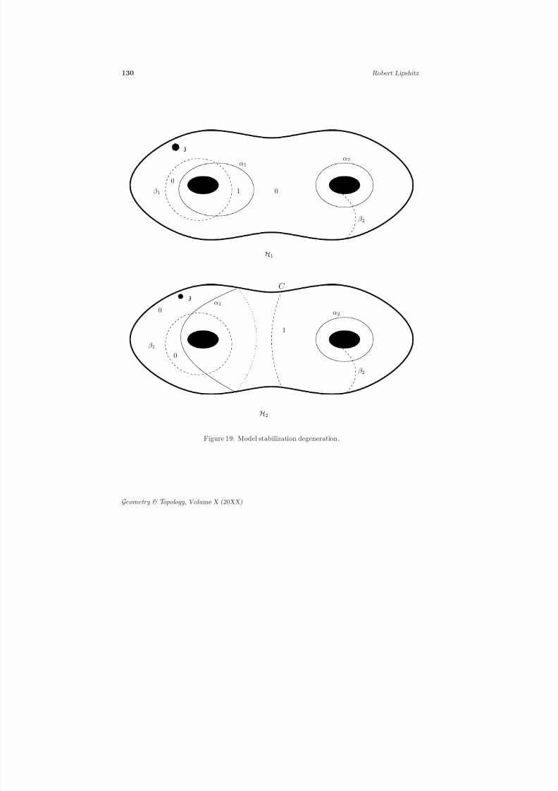
8/3/2019 Robert Lipshitz- A Cylindrical Reformulation of Heegaard Floer Homology
http://slidepdf.com/reader/full/robert-lipshitz-a-cylindrical-reformulation-of-heegaard-floer-homology 130/135
130 Robert Lipshitz
β 1
α1α2
β 2
H1
H2
β 1
α1
α2
β 2
1
0
0
1 0
0
z
z
C
Figure 19: Model stabilization degeneration.
Geometry & T opology , Volume X (20XX)
8/3/2019 Robert Lipshitz- A Cylindrical Reformulation of Heegaard Floer Homology
http://slidepdf.com/reader/full/robert-lipshitz-a-cylindrical-reformulation-of-heegaard-floer-homology 131/135
8/3/2019 Robert Lipshitz- A Cylindrical Reformulation of Heegaard Floer Homology
http://slidepdf.com/reader/full/robert-lipshitz-a-cylindrical-reformulation-of-heegaard-floer-homology 132/135
132 Robert Lipshitz
changing the wi gives bordant moduli spaces we see that # N J = ±1 for general ℓ, z0 ,
and w1, · · · , wℓ.
Since the ∂ –operator is transversal for N J , stabilization invariance now follows from thegluing result A.2 and the remark at the beginning of this proof, just as described in Propo-sition 12.5. The present proposition is also immediate. 2
B Cross–references with [21]
For the reader’s convenience I include a table indicating the correspondence between resultsin this paper and those in [21]. (The correspondence is also indicated in the text.) Thethird column indicates how similar the statements in the two places are, and the fourthhow similar the proofs are. (Both are on a scale of 0, 1, 2 or ∞, where ∞ indicates thatI refer to [21] for the proof.) The comparison is clearly rather subjective.
Geometry & T opology , Volume X (20XX)
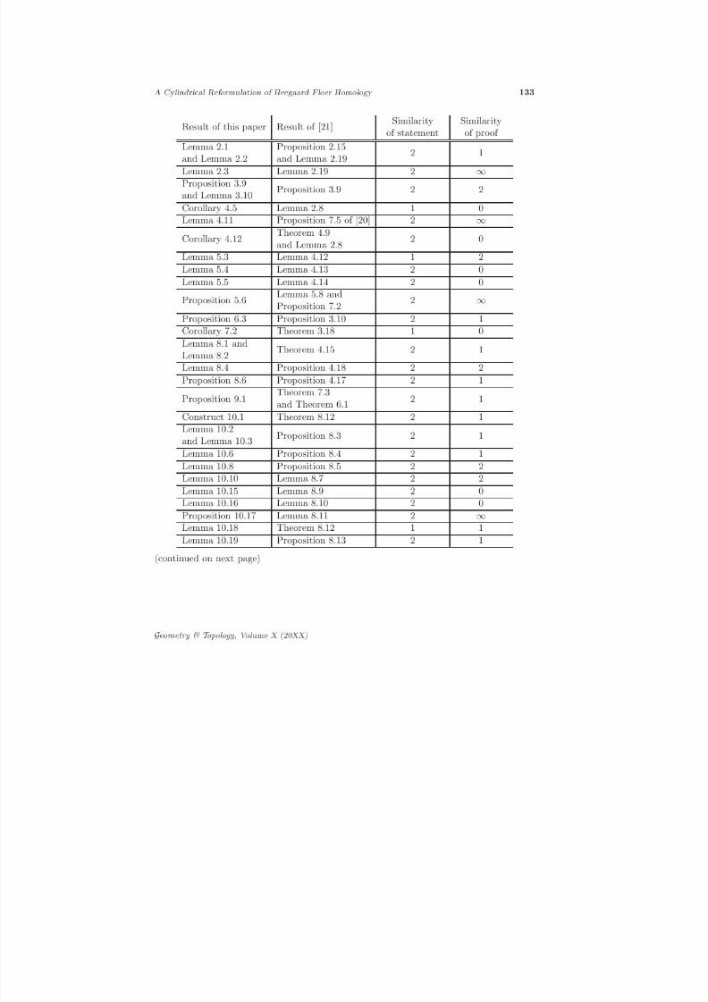
8/3/2019 Robert Lipshitz- A Cylindrical Reformulation of Heegaard Floer Homology
http://slidepdf.com/reader/full/robert-lipshitz-a-cylindrical-reformulation-of-heegaard-floer-homology 133/135
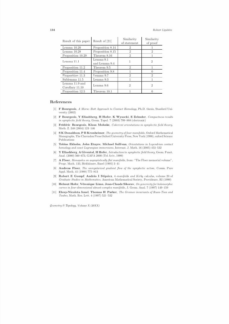
8/3/2019 Robert Lipshitz- A Cylindrical Reformulation of Heegaard Floer Homology
http://slidepdf.com/reader/full/robert-lipshitz-a-cylindrical-reformulation-of-heegaard-floer-homology 134/135
134 Robert Lipshitz
Result of this paper Result of [21]Similarity
of statement
Similarity
of proof Lemma 10.20 Proposition 8.14 2 1
Lemma 10.28 Proposition 8.15 2 2
Proposition 10.29 Theorem 8.16 2 1
Lemma 11.1Lemma 9.1and Lemma 9.4
1 2
Proposition 11.2 Theorem 9.5 2 1
Proposition 11.4 Proposition 9.8 1 0
Proposition 11.3 Lemma 9.7 2 2
Sublemma 11.5 Lemma 9.3 1 1
Lemma 11.9 and
Corollary 11.10Lemma 9.6 2 2
Proposition 12.5 Theorem 10.1 1 0
References
[1] F Bourgeois, A Morse–Bott Approach to Contact Homology , Ph.D. thesis, Stanford Uni-versity (2002)
[2] F Bourgeois, Y Eliashberg, H Hofer, K Wysocki, E Zehnder, Compactness resultsin symplectic field theory , Geom. Topol. 7 (2003) 799–888 (electronic)
[3] Frederic Bourgeois, Klaus Mohnke, Coherent orientations in symplectic field theory ,Math. Z. 248 (2004) 123–146
[4] S K Donaldson, P B Kronheimer, The geometry of four-manifolds, Oxford MathematicalMonographs, The Clarendon Press Oxford University Press, New York (1990), oxford SciencePublications
[5] Tobias Ekholm, John Etnyre, Michael Sullivan, Orientations in Legendrian contact homology and exact Lagrangian immersions, Internat. J. Math. 16 (2005) 453–532
[6] Y Eliashberg, A Givental, H Hofer, Introduction to symplectic field theory , Geom. Funct.Anal. (2000) 560–673, GAFA 2000 (Tel Aviv, 1999)
[7] A Floer, Monopoles on asymptotically flat manifolds, from: “The Floer memorial volume”,Progr. Math. 133, Birkhauser, Basel (1995) 3–41
[8] Andreas Floer, The unregularized gradient flow of the symplectic action , Comm. PureAppl. Math. 41 (1988) 775–813
[9] Robert E Gompf , Andras I Stipsicz, 4-manifolds and Kirby calculus, volume 20 of Graduate Studies in Mathematics, American Mathematical Society, Providence, RI (1999)
[10] Helmut Hofer, Veronique Lizan, Jean-Claude Sikorav, On genericity for holomorphiccurves in four-dimensional almost-complex manifolds, J. Geom. Anal. 7 (1997) 149–159
[11] Eleny-Nicoleta Ionel, Thomas H Parker, The Gromov invariants of Ruan-Tian and Taubes, Math. Res. Lett. 4 (1997) 521–532
Geometry & T opology , Volume X (20XX)

8/3/2019 Robert Lipshitz- A Cylindrical Reformulation of Heegaard Floer Homology
http://slidepdf.com/reader/full/robert-lipshitz-a-cylindrical-reformulation-of-heegaard-floer-homology 135/135


![arXiv:1112.0290v2 [math.SG] 22 Dec 2011arXiv:1112.0290v2 [math.SG] 22 Dec 2011 AN ABSOLUTE GRADING ON HEEGAARD FLOER HOMOLOGY BY HOMOTOPY CLASSES OF ORIENTED 2-PLANE FIELDS VINICIUS](https://img.pdfslide.us/doc/110x75/5f6932c2bf743a489a0f14c6/arxiv11120290v2-mathsg-22-dec-2011-arxiv11120290v2-mathsg-22-dec-2011.jpg)

![Introduction - Stanford Universitycm5/hfisums.pdf · Introduction Heegaard Floer homology is an invariant of three-manifolds introduced by Ozsv ath and Szab o in [20, 19]. By studying](https://img.pdfslide.us/doc/110x75/604e6f9a64977614b0516219/introduction-stanford-university-cm5hfisumspdf-introduction-heegaard-floer.jpg)
![Heegaard Floer homology of spatial graphsshelly/publications/HFG.pdf · Knot Floer homology, introduced by P Ozsváth and Z Szabó[18], and independently by J Rasmussen[20], is an](https://img.pdfslide.us/doc/110x75/5f0396a67e708231d409cb3e/heegaard-floer-homology-of-spatial-graphs-shellypublicationshfgpdf-knot-floer.jpg)


![A HEEGAARD-FLOER INVARIANT OF BORDERED A DISSERTATION · ([MOS]) provides an algorithm to compute CFK([ S3,K) for general K. The surgery formula of [OSd] is, therefore, a powerful](https://img.pdfslide.us/doc/110x75/5f647e4965faf6511b63f320/a-heegaard-floer-invariant-of-bordered-a-mos-provides-an-algorithm-to-compute.jpg)