Embed Size (px)
Citation preview
A coastal retracking system for satellite radar altimeter waveforms:
Application to ERS-2 around Australia
X. Deng1 and W. E. Featherstone2
Received 3 May 2005; revised 18 November 2005; accepted 3 March 2006; published 13 June 2006.
[1] Satellite radar altimeter-derived sea surface heights (SSH) are in error in coastalregions due, in part, to the complex nature of echoes returned from rapidly varying landand sea surfaces. This paper presents improved altimeter-derived SSH results inAustralian coastal regions using the waveform retracking technique, which reprocesses thewaveform data through a ‘‘coastal retracking system’’. The system, based upon asystematic analysis of satellite radar altimeter waveforms around Australia, improves SSHdata from several retrackers depending on the waveforms’ characteristics. Central tothe system is the use of two techniques: the least squares fitting and the thresholdretracking algorithms. To overcome the problem of fading noise, the fitting algorithm hasbeen developed to include a weighted iterative scheme. The retrackers include five fittingmodels and the threshold method with varying threshold levels. A waveformclassification procedure has also been developed, which enables the waveforms to besorted and then retracked by an appropriate retracker. Two cycles of 20-Hz waveform datafrom ERS-2 have been reprocessed using this system to obtain the improved SSHestimates. Using the AUSGeoid98 gravimetric geoid model as a quasi-independentreference, the system improves SSH estimates from beyond �22 km to beyond �5 kmfrom the coastline.
Citation: Deng, X., and W. E. Featherstone (2006), A coastal retracking system for satellite radar altimeter waveforms: Application
to ERS-2 around Australia, J. Geophys. Res., 111, C06012, doi:10.1029/2005JC003039.
1. Introduction
[2] The quality of sea surface height (SSH) measurementsfrom satellite radar altimetry in coastal regions is hinderednot only by less reliable geophysical and environmentalcorrections [e.g., Fernandes et al., 2003; Chelton et al.,2001], but also by the noisier radar returns from thegenerally rougher coastal sea states and simultaneousreturns from reflective land and inland water [e.g.,Mantripp, 1996; Andersen and Knudsen, 2000]. Forinstance, ERS-2 altimeter SSHs can be contaminated bythese factors up to a maximum distance of �22 km offshorethe Australian coast [Deng et al., 2002]. As such, manyscientists avoid the use of SSHs in coastal regions [e.g.,Nerem, 1995], typically beyond 20–50 km of the coast[Strub and James, 1997].[3] The profile of backscattered power (i.e., waveform)
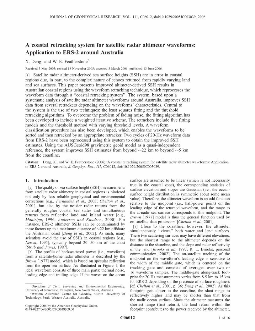
from a satellite-borne radar altimeter is described by theBrown [1977] model, which is based on specular reflectionfrom the open sea surface. As illustrated in Figure 1, theideal waveform consists of three main parts: thermal noise,leading edge and trailing edge. If the waves on the ocean
surface are assumed to be linear (which is not necessarilytrue in the coastal zone), the corresponding statistics ofsurface elevation and slopes are Gaussian (i.e., the ocean-surface height distribution is symmetric about some meanvalue). Therefore, the altimeter waveform is an odd functionrelative to the midpoint (i.e., half-power point) on theleading edge of the returned waveform, and the range tothe at-nadir sea surface corresponds to this midpoint. TheBrown [1977] model is thus the general function used byon-satellite data processors [Chelton et al., 2001].[4] Close to the coastline, however, the altimeter
simultaneously ‘‘views’’ both water and land surfaces.These two scattering surfaces may have different elevations,but the shortest range to the altimeter depends on thedistance to the shoreline, and the slope and radar reflectivityof the land [Brooks et al., 1997; R. L. Brooks, personalcommunication, 2002]. The on-satellite tracking of themidpoint on the waveform’s leading edge is sensitive tothe width of the middle gate, which is centered on thetracking gate and consists of averages over two or16 waveform samples. The middle-gate along-track foot-print for 20 Hz measurements varies from 8.5 km to 15 kmfor ERS-2 depending on the presence of surface roughness[cf. Chelton et al., 2001, p. 36; Deng et al., 2002]. As thisfootprint gets closer to the coastline, the slant range toreflectively higher land may be shorter than that fromthe nadir ocean surface. Since the altimeter measures theshortest range (first return), the land return within thefootprint contributes to the power received by the altimeter,
JOURNAL OF GEOPHYSICAL RESEARCH, VOL. 111, C06012, doi:10.1029/2005JC003039, 2006
1Discipline of Civil, Surveying and Environmental Engineering,University of Newcastle, Callaghan, New South Wales, Australia.
2Western Australian Centre for Geodesy, Curtin University ofTechnology, Perth, Western Australia, Australia.
Copyright 2006 by the American Geophysical Union.0148-0227/06/2005JC003039$09.00
C06012 1 of 16
thus contaminating the returned waveform. The shape of thewaveform can also be significantly affected by the generallyrougher coastal sea states, or from inland water. Forexample, calm (i.e., more radar-reflective) water surfacesnear the coastline, such as bays and estuaries, make thereturned power peaked. These land-contaminated andpeaked waveforms can be difficult to track using only theopen-ocean Brown [1977] model.[5] Retracking altimeter waveform data in coastal regions
to obtain improved SSHs has been the subject of compar-atively little study. Thus far, two approaches have beenapplied: the fitting and threshold techniques. The first fits ananalytical waveform model to the observed waveform datato determine more accurate range estimates [e.g.,Anzenhofer et al., 2000]. This fitting function is based uponthe 5-parameter function developed by Martin et al. [1983],choosing either a linear or an exponential trailing edge. Analternative method used by Brooks et al. [1997] is amodified threshold retracking technique [cf. Wingham etal., 1986; Davis, 1997], which retracks the ocean returnfrom the land-contaminated waveforms close to the coast-line. To the authors’ knowledge, most previously publishedretracking efforts in coastal zones use algorithms developedfor ice sheets, and only a single retracker is used. However,it will be shown in this paper that using only a singleretracker limits the precision of recovered SSHs due to thediverse waveform shapes in coastal regions.[6] A comprehensive analysis of waveform shapes at the
Australian coast led to the need to develop a ‘‘coastalwaveform retracking system’’. The primary idea behindthe system is that several retrackers must deal with themajority of the coastal waveforms, and they must comple-ment one another. As a case study, the system is applied tothe Australian coast using two cycles (42 and 43) of ERS-220 Hz waveform data (March to May 1999). The SSHbefore and after retracking is compared with an externalquasi-independent reference of the AUSGeoid98 gravimet-ric geoid model [Featherstone et al., 2001], which verifies
the effectiveness of the system. The term quasi-independentreflects that altimeter-derived gravity anomalies were one ofthe data sources for this model.[7] It is acknowledged that the instantaneous SSH is not
equivalent to the geoid (loosely mean sea level). Thedifference between them includes the time-variant compo-nent (e.g., tides) and the time-invariant component (e.g., theocean surface mean dynamic topography (MDT)). Theformer can be removed by averaging, and the latter canbe removed by a MDT correction to the SSH. However, theMDT models are usually designed for resolving basin-widescales and hence are highly smoothed [e.g., Levitus, 1982].Applying such a MDT correction in coastal regions maycause an additional error to the SSH, which might be largerthan the errors of other geophysical and environmentalcorrections. Therefore, the MDT was not applied to theSSH data in this study. Assuming that the MDT is a bias inthe coastal zone, the verification of any improvement in theSSH will be seen in the standard deviations (STD) of themean difference, with a smaller value indicating an im-provement in the SSH.
2. Costal Waveform Retracking Design andImplementation
2.1. System Design
[8] Retracking is a procedure of waveform data post-processing that aims to improve parameter estimates overthose given as part of the standard altimeter ‘‘geophysicaldata products’’. These parameters include the range correc-tion due to the estimation algorithm used and the limitedcomputational time on board the satellite [e.g., Hayne,1980; Rodriguez, 1988]. It is determined through estimatingthe offset of the actual tracking gate, which is related to themidpoint on the leading edge (see Figure 1), from the pre-designed tracking gate that is used by default during on-satellite processing. This correction is then applied to therange calculated by the onboard algorithm.[9] Because of the presence of various waveform shapes
in coastal regions (see section 3.2), a coastal waveformretracking system, which consists of different retrackingalgorithms, should be considered when attempting to extractthe precise SSHs from these land-contaminated waveforms.We have found that these are the fitting functions of theocean, 5- and 9-parameter models, and threshold retrackingalgorithm (see Appendix A).[10] The ocean model (equation (A1)), without the non-
linear ocean wave parameter, has been used as a mainretracker in this system due to its clearly physical descrip-tion of the ocean surface. By quantitative comparison to the5-parameter model (equations (A6) and (A9)), the slope ofthe trailing edge modeled by the 5-parameter model has alarger range of variation than the ocean model (see Appen-dix B). This advantage makes the 5-parameter model morecapable of fitting non-ocean-like or irregular waveforms incoastal regions than the ocean model. Thus, the 5-parametermodel replaces the ocean model for irregular-shaped wave-forms in our system.[11] To deal with peaked waveforms reflected from calm
coastal or inland water surfaces, the threshold retrackingtechnique with 50% threshold level (Appendix A2) wasused. However, it is found that the 50% threshold level
Figure 1. Schematic altimeter mean return waveform oversea surfaces. The ERS-2 waveform is recorded in 64 rangebins or gates. The spacing of the gates is 3.03 nsec or 454mm. The leading edge usually spans 3–4 range bins.
C06012 DENG AND FEATHERSTONE: A COASTAL ALTIMETRY RETRACKING SYSTEM
2 of 16
C06012
cannot always give improved results, particularly in the areaclosest to the coastline where peaked waveforms are moreprevalent. To validate the appropriate threshold level, astatistical analysis was performed to suggest the quality ofthe retracked SSH data. This turned out a detailed selectionof the appropriate threshold levels (see section 2.3). A
variable threshold level of 50% or 30% depending on thewaveform shape is finally used in the system.[12] Since valid SSH data can only be recovered from
ocean returns, it is not necessary for our system to reprocesswaveforms dominated by land returns. However, it issignificant that the system can correctly categorize the
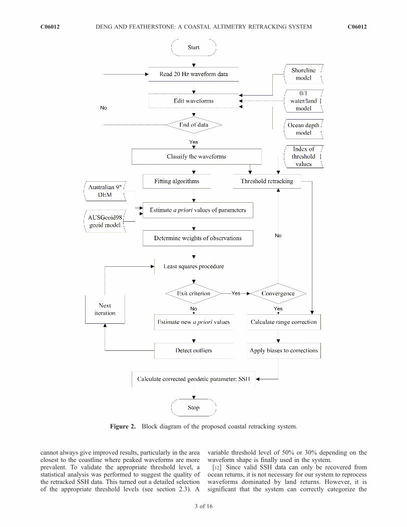
Figure 2. Block diagram of the proposed coastal retracking system.
C06012 DENG AND FEATHERSTONE: A COASTAL ALTIMETRY RETRACKING SYSTEM
3 of 16
C06012
waveforms, so that they can be retracked using a moreappropriate retracker. This has generated an additionalwaveform classification stage to sort waveforms based ontheir different shapes, and thus indicate which retrackershould be used for each. When retracking costal waveformsusing all possible retrackers, improved SSHs result, butbiases exist among different algorithms. Thus, an algorithmassessment has been implemented to analyze and estimatethese biases (see section 2.4).[13] Finally, Figure 2 illustrates how coastal waveforms
are reprocessed to give the corrected SSH data: a specificretracker (fitting or threshold) is applied to each waveformbased upon the earlier classification. When using the fittingalgorithm, an adequate fitting function must be selected andthe iterative nonlinear fitting procedure is used. Since alinear solution to a non-linear problem is sought, the fittingalgorithm does not always work [Zwally et al., 1990; Davis,1995]. Therefore, the threshold retracking replaces theiterative least squares fit to compute the retracking correc-tion if and when the fitting procedure fails. Thresholdretracking works both for peaked waveforms and those thatfail with the fitting algorithm. Also, the system automati-cally selects the appropriate threshold level for each wave-form depending on its categorized shape.
2.2. Data Weighting and Outlier Detecting
[14] An appropriate weight scheme is essential whenusing the fitting algorithm. In general, the trailing edgeshows more obvious undulations than any other parts of thewaveform due to the ‘‘fading’’ noise, which is caused by theincoherent superposition of signals from different reflectingfacets [Partington et al., 1991; Quartly and Srokosz, 2001].The noise in the trailing edge greatly influences the iterativefitting procedure and accurate results may not be estimated.To solve this problem, two approaches are usually used. Thefirst is to average waveforms in the time span of severalseconds to reduce noise, and then to fit a model to thisaveraged waveform [e.g., Hayne and Hancock, 1990;Fairhead et al., 2001]. The second is to give less weight
to the waveform samples in the trailing edge [Zwally et al.,1990; Brenner et al., 1993; Anzenhofer et al., 2000].[15] However, the averaging procedure is not always
appropriate in coastal regions, because true ocean wave-forms will be distorted by land-contaminated waveformswithin the averaging window. The approach of downweighting the trailing edge, such as the a priori weights(pi
0) scheme used by Anzenhofer et al. [2000], cannotcompletely overcome the problem caused by undulationsin the trailing edge. Therefore, an outlier detection approachfrom an iterative weight scheme was developed and used.[16] In this iterative procedure, the initial least squares
adjustment is conducted using the a priori values and apriori weights (pi
0). After the first adjustment, a new weightfunction wi is given as [e.g., Li, 1988]
wi ¼
1
vij j for vij j > 0:7s0
1
0:7s0for vij j � 0:7s0
8>><>>:
ð1Þ
where vi and s02 are estimates of the parameter correction
vector and unit weight variance, respectively. The next stepthen is to determine the weight (pi
j+1) for the nextadjustment using wi as follows:
pjþ1i ¼ p
ji wi ð2Þ
where j means the j-th iteration in the adjustment. In themeantime, the parameter estimates take the place of theoriginal estimates; the entire cycle is repeated to produceimproved estimates. In this way, the observations consid-ered to contain the outlier will be downweighted but still bekept in the data set, while non-outlier observations willmaintain full weight after each iterative cycle.
2.3. Selection of the Threshold Level
[17] There are two concerns related to the selection of thethreshold level. The first is that threshold values should behigher than both the noise and the spectral leakage in thestart/end gates. The second is that the values should besufficiently lower than the sought-after ocean returns.Brooks et al. [1997] determine different threshold valuesfor 18 TOPEX ground tracks near land based upon a visualexamination method. These values were then used to retrackthe coastal waveform along the same satellite pass. Thismethod is advantageous because it accounts for the powerbackscattered from different reflecting surfaces. However,because an automatic selection of the threshold level is notavailable, this restrains the technique from retracking thewide range of waveforms in coastal regions.[18] Considering the various waveform shapes in the
coasts, four threshold schemes are investigated beforearriving at the final threshold level in this study. They areas follows: (a) Fixed counts, which is defined as 50% of themean-waveform amplitude in counts. (b) 50% of the wave-form amplitude. (c) 30% and 50% of the waveform ampli-tude. The 30% waveform amplitude is selected to retrackwaveforms within 0–5 km from the coasts, while the 50%of the waveform amplitude is used after 5 km. (d) Variablethreshold level. If the waveform classification indicates a
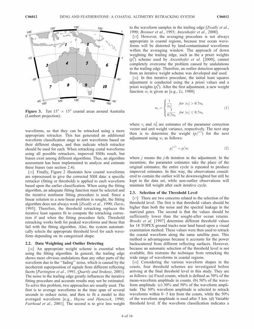
Figure 3. Ten 15� � 15� coastal areas around Australia(Lambert projection).
C06012 DENG AND FEATHERSTONE: A COASTAL ALTIMETRY RETRACKING SYSTEM
4 of 16
C06012
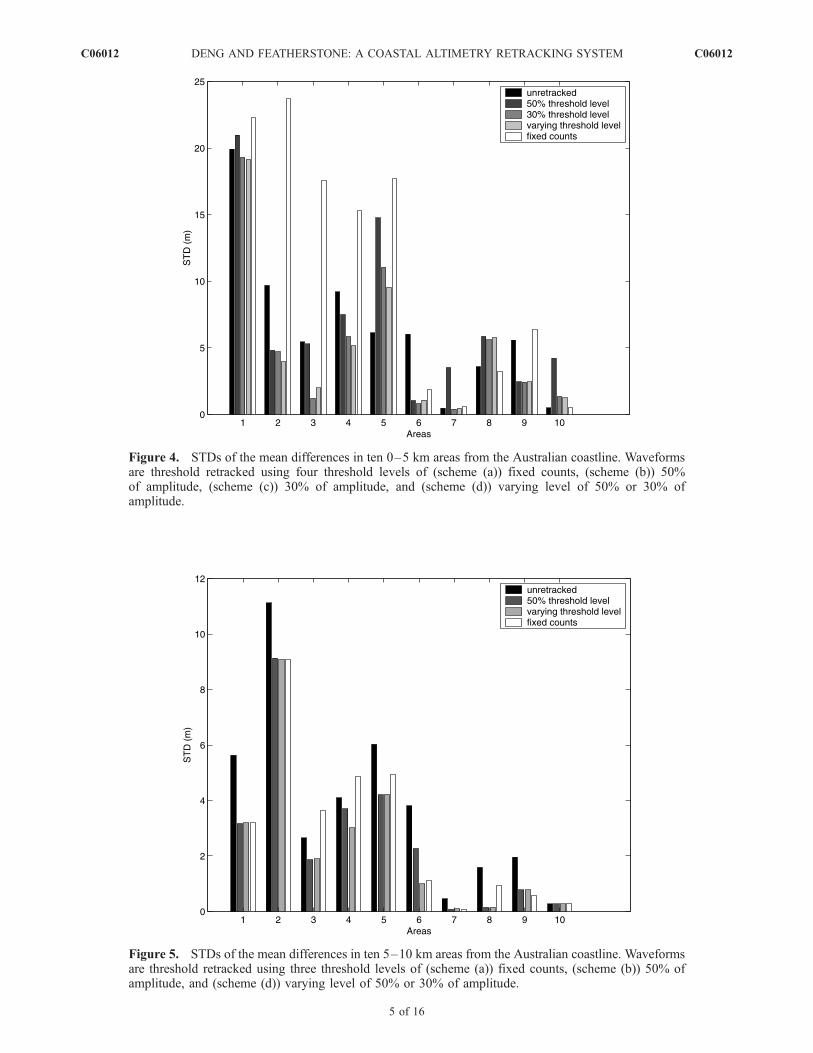
Figure 4. STDs of the mean differences in ten 0–5 km areas from the Australian coastline. Waveformsare threshold retracked using four threshold levels of (scheme (a)) fixed counts, (scheme (b)) 50%of amplitude, (scheme (c)) 30% of amplitude, and (scheme (d)) varying level of 50% or 30% ofamplitude.
Figure 5. STDs of the mean differences in ten 5–10 km areas from the Australian coastline. Waveformsare threshold retracked using three threshold levels of (scheme (a)) fixed counts, (scheme (b)) 50% ofamplitude, and (scheme (d)) varying level of 50% or 30% of amplitude.
C06012 DENG AND FEATHERSTONE: A COASTAL ALTIMETRY RETRACKING SYSTEM
5 of 16
C06012
distorted waveform, the threshold level is set to 30% (or20% depending on the reflecting surface); otherwise the50% of waveform amplitude is set.[19] In order to ascertain the appropriate threshold level,
one cycle of 20 Hz ERS-2 waveform data (March to April1999) in ten 15� � 15� areas around the Australian coastwere used (Figure 3). The AUSGeoid98 gravimetric geoidmodel [Featherstone et al., 2001] was used as external‘‘ground truth’’ for the comparisons. Waveforms werethreshold-retracked using the above four schemes. For eachalong-track altimeter SSH after retracking, the griddedAUSGeoid98 geoid height was bi-spline-interpolated tothe longitude and latitude of the altimeter ground point.Descriptive statistics were computed from the differencebetween the SSH and geoid height. Figures 4 and 5show STDs of mean differences in two distance bands of0–5 km and 5–10 km around Australia’s coasts (Figure 3),respectively.[20] In both Figures 4 and 5, STDs are large in most of
the areas before retracking. In the 0–5 km distance band(Figure 4), after threshold retracking using scheme (b), theSTD decreases in five areas, but increases in the other five.The reason for this is that the mostly varying land topog-raphy and still water can heavily contaminate the wave-forms, so that many waveform shapes do not follow theocean model. This suggests that the 50% threshold level isnot an appropriate selection for the waveforms within 5 kmof the coast. After retracking using schemes (c) and (d), theSTD shows improvements in seven areas. Of them, theresults from the scheme (d) show the most significantimprovement. In contrast, scheme (a) gives the least im-provement, and even worse results in most areas afterretracking. For areas 5, 8 and 10, an appropriate thresholdlevel of 20% was found. As can be seen from the ordinatescale in Figure 5 (5–10 km distance band), STDs decreasewith increasing the distance from the coasts. All schemes,except for scheme (a), show similar results in most areas.This implies that less waveform contamination occurs inthese areas, which agrees with results by Deng et al. [2002].[21] The count-fixed level (scheme a) cannot follow the
variations in the scattering surfaces. It assumes that theretracking amplitude of the ocean waveform does notchange with varying surface roughness or topography.However, this is not the actual case, even over oceansurfaces. The 50% threshold retracking level (scheme b) isset too high to capture the ocean returns for the contami-nated waveforms in coasts. Setting the 30% threshold levelwithin 5 km from the coast and the 50% threshold beyond5 km (scheme c) presents an improved result, but causes astep in the ranges after retracking where the threshold levelsuddenly changes. Nevertheless, the 30% (or 20% in some
areas) and 50% threshold levels (scheme d) over large areasof the coastal regions appear more reasonable (Figures 4and 5).
2.4. Assessment of Biases Among RetrackingAlgorithms
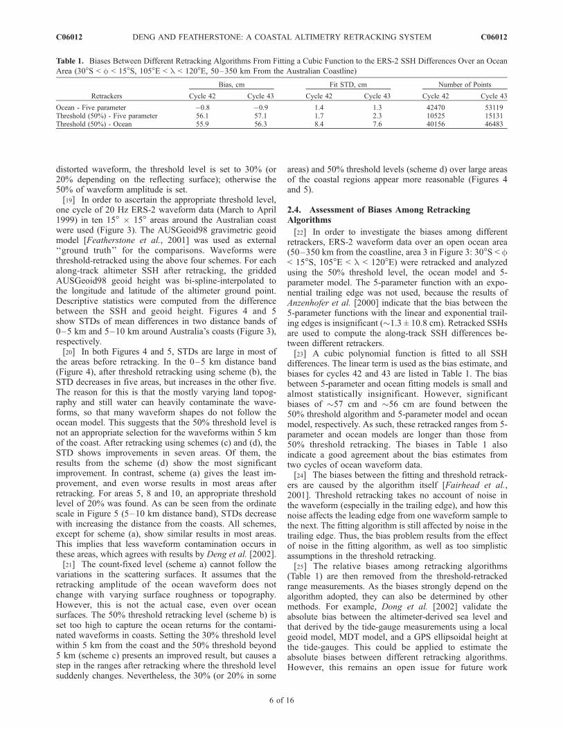
[22] In order to investigate the biases among differentretrackers, ERS-2 waveform data over an open ocean area(50–350 km from the coastline, area 3 in Figure 3: 30�S < f< 15�S, 105�E < l < 120�E) were retracked and analyzedusing the 50% threshold level, the ocean model and 5-parameter model. The 5-parameter function with an expo-nential trailing edge was not used, because the results ofAnzenhofer et al. [2000] indicate that the bias between the5-parameter functions with the linear and exponential trail-ing edges is insignificant (�1.3 ± 10.8 cm). Retracked SSHsare used to compute the along-track SSH differences be-tween different retrackers.[23] A cubic polynomial function is fitted to all SSH
differences. The linear term is used as the bias estimate, andbiases for cycles 42 and 43 are listed in Table 1. The biasbetween 5-parameter and ocean fitting models is small andalmost statistically insignificant. However, significantbiases of �57 cm and �56 cm are found between the50% threshold algorithm and 5-parameter model and oceanmodel, respectively. As such, these retracked ranges from 5-parameter and ocean models are longer than those from50% threshold retracking. The biases in Table 1 alsoindicate a good agreement about the bias estimates fromtwo cycles of ocean waveform data.[24] The biases between the fitting and threshold retrack-
ers are caused by the algorithm itself [Fairhead et al.,2001]. Threshold retracking takes no account of noise inthe waveform (especially in the trailing edge), and how thisnoise affects the leading edge from one waveform sample tothe next. The fitting algorithm is still affected by noise in thetrailing edge. Thus, the bias problem results from the effectof noise in the fitting algorithm, as well as too simplisticassumptions in the threshold retracking.[25] The relative biases among retracking algorithms
(Table 1) are then removed from the threshold-retrackedrange measurements. As the biases strongly depend on thealgorithm adopted, they can also be determined by othermethods. For example, Dong et al. [2002] validate theabsolute bias between the altimeter-derived sea level andthat derived by the tide-gauge measurements using a localgeoid model, MDT model, and a GPS ellipsoidal height atthe tide-gauges. This could be applied to estimate theabsolute biases between different retracking algorithms.However, this remains an open issue for future work
Table 1. Biases Between Different Retracking Algorithms From Fitting a Cubic Function to the ERS-2 SSH Differences Over an Ocean
Area (30�S < f < 15�S, 105�E < l < 120�E, 50–350 km From the Australian Coastline)
Retrackers
Bias, cm Fit STD, cm Number of Points
Cycle 42 Cycle 43 Cycle 42 Cycle 43 Cycle 42 Cycle 43
Ocean - Five parameter 0.8 0.9 1.4 1.3 42470 53119Threshold (50%) - Five parameter 56.1 57.1 1.7 2.3 10525 15131Threshold (50%) - Ocean 55.9 56.3 8.4 7.6 40156 46483
C06012 DENG AND FEATHERSTONE: A COASTAL ALTIMETRY RETRACKING SYSTEM
6 of 16
C06012
because of limited availability of such data at the time ofthis study.
3. Application to the Australian Coast
3.1. Data and Editing
[26] As well as two cycles of ERS-2 20 Hz waveformdata, external data were used to provide information neces-sary for data editing and valuation. They are the GSHHS(0.2 km resolution) shoreline model [Wessel and Smith,1996], the Australian DEM (900 � 900 resolution, version 2),the DS759.2 (50 � 50 resolution) ocean depth model
[Dunbar, 2000], the Australian bathymetric model (3000
resolution) [Buchanan, 1991], and the AUSGeoid98 (20 �20 resolution) gravimetric geoid model [Featherstone et al.,2001]. As stated, the MDT is not applied to the SSH data inthis study, so any improvement in the SSH will only be seenin the STD.[27] After retracking, geophysical corrections supplied
with the waveform data by NRSC [1995] were applied toboth retracked and unretracked range measurements toobtain the SSH. Since the electromagnetic (EM) biascorrection caused by ocean surface waves is not supplied
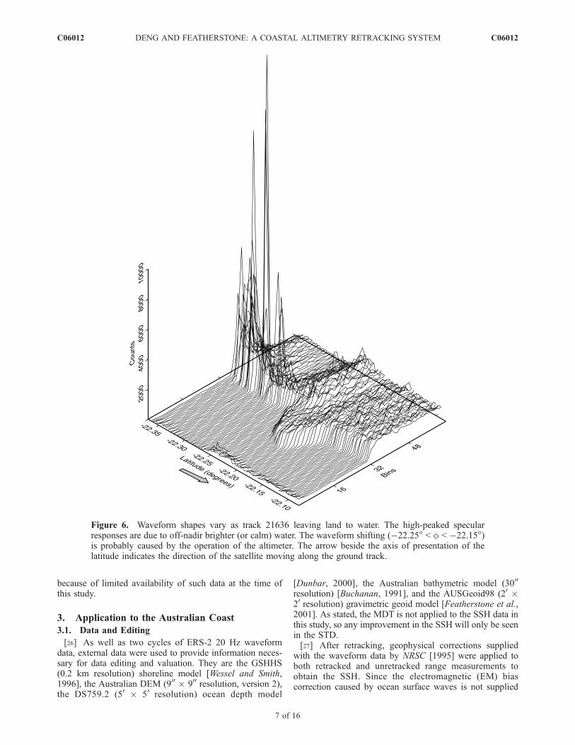
Figure 6. Waveform shapes vary as track 21636 leaving land to water. The high-peaked specularresponses are due to off-nadir brighter (or calm) water. The waveform shifting (22.25� < f < 22.15�)is probably caused by the operation of the altimeter. The arrow beside the axis of presentation of thelatitude indicates the direction of the satellite moving along the ground track.
C06012 DENG AND FEATHERSTONE: A COASTAL ALTIMETRY RETRACKING SYSTEM
7 of 16
C06012
with the waveform data products used in this study, it wasnot applied to the range measurements. Neither were theDoppler range corrections applied because most valueswere found to exceed the error criterion of ±55 cm givenby NRSC [1995].
3.2. Waveform Classification
[28] Contaminated waveforms [cf. Deng et al., 2002]around the Australian coast have been categorized, whichis needed to choose the appropriate retracking algorithm. Adetailed example of typical waveform categorization isgiven here from one ascending ground track 21636 off thenorthwest Australian coast (Figure 6). It is important toobserve the departure of the mid-point on the waveform’sleading edge from the expected tracking gate (i.e., 32.5 forERS-2).[29] Figure 6 shows ascending pass 21636 going from
land to water. The waveforms present different shapes, suchas high-peaked and land-contaminated, and then a change totypical ocean shapes at around 22.1� latitude. The wave-form shifting in the range window is clear, which isprobably due to the change of operation modes of thealtimeter at the coast [Deng, 2004]. For most of thecontaminated waveforms (Figure 6), a distinct leading edgeis observable; in some cases, double ramps are apparent,
and in others, high peaks with sharp ramp and rapidlydecreasing trailing edge are apparent.[30] The contaminated waveforms in ten 15� � 15�
Australian coastal regions (Figure 3) are categorized inTable 2. Most contaminated waveforms (80.19%) haveocean-like shapes. The mean width of these waveforms issimilar to that of ocean waveforms, whereas the mean peakvalue is larger. The remaining waveforms have single pre-peaked (4.65%) and high-peaked (4.35%) waveformshapes. Others, such as single mid-peaked and post-peaked,double pre-peaked and post-peaked, and multi-peakedwaveforms, fall in the range 0.73%–1.35%. Although thereis only a small percentage (12.34%) of non-ocean-likewaveforms, they are found closer to the coastline (1.73–3.12 km on average), indicating further that a retrackingsystem containing several retrackers is necessary.[31] In addition, from waveform categorization, high-
peaked waveforms take a larger percentage of contaminatedwaveforms (from 5.4% to 6.9%) in north-west Australiancoastal areas 1, 3 and 4 in Figure 3 because of the ruggedcoastline, complex sea states and inland/standing water[Thom, 1984].[32] The percentages of waveforms retracked by fitting
and threshold algorithms are listed in Table 3. It can be seenthat 81% to 96% of waveforms in the study area can beretracked by the least squares fitting algorithm. The rest of
Table 2. Statistics of ERS-2 (Cycle 42) Contaminated Waveform Shapes in Ten Australian Coastal Areas (See
Figure 3)
WaveformCategories
Percent ofWaveforms
MeanDistance FromCoastline,
km
Mean Width ofWaveforms,
Bins
Mean Peak ofWaveforms,Counts
Oceana 99.97 168.04 25.8 1304.1Ocean-like 80.19 10.50 24.9 1380.3Single pre-peaked 4.64 2.31 10.7 2785.1Single mid-peaked 0.54 2.54 9.8 2615.0Single post-peaked 1.35 3.12 11.8 3027.0Double pre-peaked 0.55 3.08 14.8 2280.9Double post-peaked 0.73 2.15 16.1 2271.9Multi-peaked 0.18 2.30 13.0 2117.5Sharp/High-peaked 4.35 1.73 3.3 8439.5Unusable 7.51 6.03 34.7 1234.6
aOcean waveforms over open oceans 50–350 km from the coastline, with 50% threshold retracking point estimates betweenbins/gates 31–33.
Table 3. Waveform Data Status and Percentage of the Waveforms Retracked Using Fitting and Threshold
Retracking Algorithms in Australian Coastal Regions (Cycles 42 and 43)
AreaNumber Areasa
Number ofData
Unusual Data,%
Fit,%
Threshold,%
1 120� � l < 135�, 15�� f < 0� 10752 1.5 82.9 15.72 135� � l < 150�, 15� � f < 0� 10922 1.7 85.5 12.83 105� � l < 120�, 30� � f < 15� 13448 1.7 86.5 8.64 120� � l < 135�, 30� � f < 15� 6065 2.2 80.9 16.85 135� � l < 150�, 30� � f < 15� 9682 2.1 88.0 9.46 150� � l < 165�, 30� � f < 15� 3739 0.2 92.8 7.07 105� � l < 120�, 45� � f < 30� 6055 7.4 88.6 4.68 120� � l < 135�, 45� � f < 30� 12288 4.3 88.8 6.99 135� � l < 150�, 45� � f < 30� 21672 2.6 90.3 7.110 150� � l < 165�, 45� � f < 30� 4115 0.0 95.6 4.4aHere f and l are the latitude and longitude, respectively (see Figure 3).
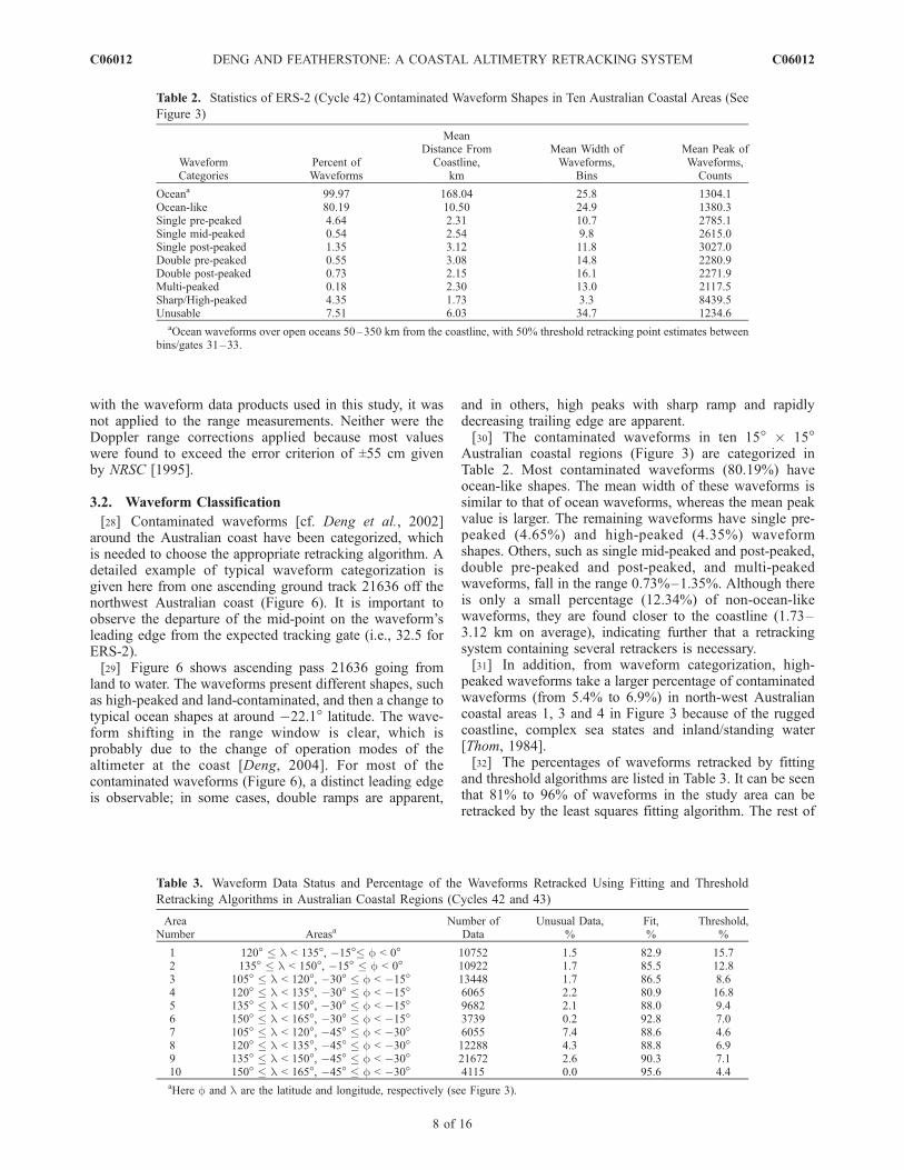
C06012 DENG AND FEATHERSTONE: A COASTAL ALTIMETRY RETRACKING SYSTEM
8 of 16
C06012
the waveforms (the last column) still require thresholdretracking (�4% to �17% for both cycles). The percentagesof different retrackers used vary from area to area dependingon the reflecting surface topography. As to the fittingalgorithm from Table 3, �98.5% of waveforms can befitted by the ocean or 5-parameter models. A maximum1% of waveforms are fitted using the 5-parameter modelwith an exponential trailing edge. In addition, a maximum0.4% of waveforms are fitted by the 9-parameter model witheither a linear or an exponential trailing edge.[33] The statistics corresponding to six 5-km-wide dis-
tance bands from the coastline has also been calculated.According to the results of both cycles, 65% and 35% ofwaveforms are retracked by the fitting and threshold algo-rithms in a distance band of 0–5 km, respectively. From 5–10 km, 96% and 4% of waveforms were retracked by thefitting and threshold algorithms, respectively. As to the restof four distance bands from 10 km to 30 km, 98% wave-forms were retracked by the fitting algorithm, while 2%needed to be threshold retracked. Overall, the waveformshapes generally agree well with the typical ocean wave-form beyond 10 km offshore.
3.3. Analysis of the SSH Data Before andAfter Retracking
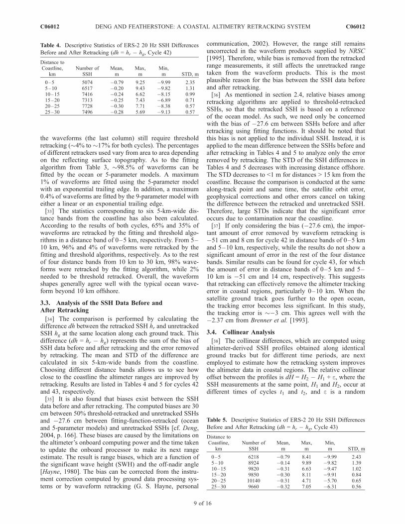
[34] The comparison is performed by calculating thedifference dh between the retracked SSH hr and unretrackedSSH hg at the same location along each ground track. Thisdifference (dh = hr hg) represents the sum of the bias ofSSH data before and after retracking and the error removedby retracking. The mean and STD of the difference arecalculated in six 5-km-wide bands from the coastline.Choosing different distance bands allows us to see howclose to the coastline the altimeter ranges are improved byretracking. Results are listed in Tables 4 and 5 for cycles 42and 43, respectively.[35] It is also found that biases exist between the SSH
data before and after retracking. The computed biases are 30cm between 50% threshold-retracked and unretracked SSHsand 27.6 cm between fitting-function-retracked (oceanand 5-parameter models) and unretracked SSHs [cf. Deng,2004, p. 166]. These biases are caused by the limitations onthe altimeter’s onboard computing power and the time takento update the onboard processor to make its next rangeestimate. The result is range biases, which are a function ofthe significant wave height (SWH) and the off-nadir angle[Hayne, 1980]. The bias can be corrected from the instru-ment correction computed by ground data processing sys-tems or by waveform retracking (G. S. Hayne, personal
communication, 2002). However, the range still remainsuncorrected in the waveform products supplied by NRSC[1995]. Therefore, while bias is removed from the retrackedrange measurements, it still affects the unretracked rangetaken from the waveform products. This is the mostplausible reason for the bias between the SSH data beforeand after retracking.[36] As mentioned in section 2.4, relative biases among
retracking algorithms are applied to threshold-retrackedSSHs, so that the retracked SSH is based on a referenceof the ocean model. As such, we need only be concernedwith the bias of 27.6 cm between SSHs before and afterretracking using fitting functions. It should be noted thatthis bias is not applied to the individual SSH. Instead, it isapplied to the mean difference between the SSHs before andafter retracking in Tables 4 and 5 to analyze only the errorremoved by retracking. The STD of the SSH differences inTables 4 and 5 decreases with increasing distance offshore.The STD decreases to <1 m for distances > 15 km from thecoastline. Because the comparison is conducted at the samealong-track point and same time, the satellite orbit error,geophysical corrections and other errors cancel on takingthe difference between the retracked and unretracked SSH.Therefore, large STDs indicate that the significant erroroccurs due to contamination near the coastline.[37] If only considering the bias (27.6 cm), the impor-
tant amount of error removed by waveform retracking is51 cm and 8 cm for cycle 42 in distance bands of 0–5 kmand 5–10 km, respectively, while the results do not show asignificant amount of error in the rest of the four distancebands. Similar results can be found for cycle 43, for whichthe amount of error in distance bands of 0–5 km and 5–10 km is 51 cm and 14 cm, respectively. This suggeststhat retracking can effectively remove the altimeter trackingerror in coastal regions, particularly 0–10 km. When thesatellite ground track goes further to the open ocean,the tracking error becomes less significant. In this study,the tracking error is �3 cm. This agrees well with the2.37 cm from Brenner et al. [1993].
3.4. Collinear Analysis
[38] The collinear differences, which are computed usingaltimeter-derived SSH profiles obtained along identicalground tracks but for different time periods, are nextemployed to estimate how the retracking system improvesthe altimeter data in coastal regions. The relative collinearoffset between the profiles is dH = H2 H1 + e, where theSSH measurements at the same point, H1 and H2, occur atdifferent times of cycles t1 and t2, and e is a random
Table 4. Descriptive Statistics of ERS-2 20 Hz SSH Differences
Before and After Retracking (dh = hr hg, Cycle 42)
Distance toCoastline,
kmNumber of
SSHMean,m
Max,m
Min,m STD, m
0–5 5074 0.79 9.25 9.99 2.355–10 6517 0.20 9.43 9.82 1.3110–15 7416 0.24 6.62 8.15 0.9915–20 7313 0.25 7.43 6.89 0.7120–25 7728 0.30 7.71 8.38 0.5725–30 7496 0.28 5.69 9.13 0.57
Table 5. Descriptive Statistics of ERS-2 20 Hz SSH Differences
Before and After Retracking (dh = hr hg, Cycle 43)
Distance toCoastline,
kmNumber of
SSHMean,m
Max,m
Min,m STD, m
0–5 6218 0.79 8.41 9.99 2.435–10 8924 0.14 9.89 9.82 1.3910–15 9820 0.31 6.63 9.47 1.0215–20 9850 0.30 8.11 9.91 0.8420–25 10140 0.31 4.71 5.70 0.6525–30 9660 0.32 7.05 6.31 0.56
C06012 DENG AND FEATHERSTONE: A COASTAL ALTIMETRY RETRACKING SYSTEM
9 of 16
C06012
measurement error. In this study, since cycle 43 containsmore orbits and thus more complete data coverage, it ischosen as a reference. SSH data from cycle 42 are thenreduced to relevant points along ground tracks of cycle 43.The cross-track geoid gradient correction [cf. Wang andRapp, 1991] is not applied, because data came from twoadjacent cycles and the effects of the geoid slope can beneglected.[39] The collinear differences remove the long-wave-
length geoid and MDT as well as variations of the oceansurface, representing thus the amount of orbit error, altim-eter range measurement error and temporal variations of thesurface over oceans. In coastal regions, the random erroralso includes the tracking error caused by coastal topogra-phy. After removing the satellite orbit error, SSH data fromrepeat cycles can also be used to determine the mean seasurface [Wang and Rapp, 1991; Nerem, 1995]. Thus, theSTD of dH is used as a measure of the quality of aretracking algorithm’s range estimate. If errors caused bywaveform contamination can be removed by retracking, thiswill result in smaller STDs.[40] The descriptive statistics of the collinear 20 Hz SSH
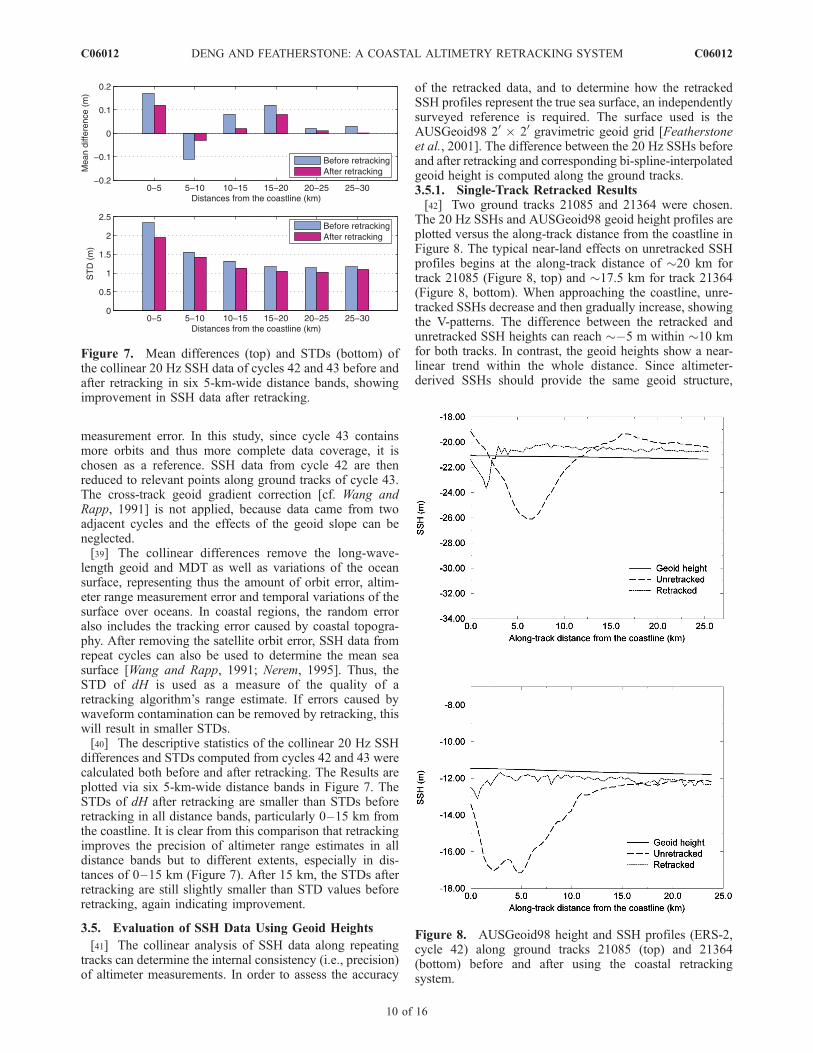
differences and STDs computed from cycles 42 and 43 werecalculated both before and after retracking. The Results areplotted via six 5-km-wide distance bands in Figure 7. TheSTDs of dH after retracking are smaller than STDs beforeretracking in all distance bands, particularly 0–15 km fromthe coastline. It is clear from this comparison that retrackingimproves the precision of altimeter range estimates in alldistance bands but to different extents, especially in dis-tances of 0–15 km (Figure 7). After 15 km, the STDs afterretracking are still slightly smaller than STD values beforeretracking, again indicating improvement.
3.5. Evaluation of SSH Data Using Geoid Heights
[41] The collinear analysis of SSH data along repeatingtracks can determine the internal consistency (i.e., precision)of altimeter measurements. In order to assess the accuracy
of the retracked data, and to determine how the retrackedSSH profiles represent the true sea surface, an independentlysurveyed reference is required. The surface used is theAUSGeoid98 20 � 20 gravimetric geoid grid [Featherstoneet al., 2001]. The difference between the 20 Hz SSHs beforeand after retracking and corresponding bi-spline-interpolatedgeoid height is computed along the ground tracks.3.5.1. Single-Track Retracked Results[42] Two ground tracks 21085 and 21364 were chosen.
The 20 Hz SSHs and AUSGeoid98 geoid height profiles areplotted versus the along-track distance from the coastline inFigure 8. The typical near-land effects on unretracked SSHprofiles begins at the along-track distance of �20 km fortrack 21085 (Figure 8, top) and �17.5 km for track 21364(Figure 8, bottom). When approaching the coastline, unre-tracked SSHs decrease and then gradually increase, showingthe V-patterns. The difference between the retracked andunretracked SSH heights can reach �5 m within �10 kmfor both tracks. In contrast, the geoid heights show a near-linear trend within the whole distance. Since altimeter-derived SSHs should provide the same geoid structure,
Figure 7. Mean differences (top) and STDs (bottom) ofthe collinear 20 Hz SSH data of cycles 42 and 43 before andafter retracking in six 5-km-wide distance bands, showingimprovement in SSH data after retracking.
Figure 8. AUSGeoid98 height and SSH profiles (ERS-2,cycle 42) along ground tracks 21085 (top) and 21364(bottom) before and after using the coastal retrackingsystem.
C06012 DENG AND FEATHERSTONE: A COASTAL ALTIMETRY RETRACKING SYSTEM
10 of 16
C06012
but different noise components from observations, suchlarge differences with respect to the geoid clearly showsthe general waveform contamination problem that exists inthe untracked SSH data.[43] In addition, according to the shape of the unretracked
SSH profiles, the along-track SSH and corresponding geoidgradients were computed. The results from track 21085(Figure 8, top) show that along-track AUSGeoid98 geoidgradients are small, from 9.2 to 10.9 ppm (mm/km) whenthe ground track is 0–7.5 km and 7.6–19.5 km from thecoastline. For the same distances, unretracked-SSH gra-dients are 975.6 ppm and 509.2 ppm. Since the maximumgeoid gradient is �150 ppm in Australia [cf. Friedlieb et al.,1997; Featherstone et al., 2001], such SSH gradients areunrealistic and thus due to onboard tracking algorithmerrors. Beyond 19.5 km from the coastline, AUSGeoid98and unretracked-SSH gradients show commensurately smallvalues of 12.5 ppm and 6.4 ppm. For track 21364 (Figure8, bottom), unretracked-SSH gradients are of 803.3 ppmand 363.8 ppm. The relative SSH gradients decrease to�16.0 ppm after retracking for both tracks. Together, theseresults suggest as well that unretracked SSHs are in errorwithin an along-track distance of 0–19.5 km from thecoastline for tracks 21085 and 21364.[44] Our retracking system, comprising several retrackers,
can improve the SSH profile shoreward several kilometers,say �10–15 km from the coastline in Figure 8. Comparingthe SSH profiles before and after retracking in Figure 8, theSSH profiles after retracking show a good agreement withthe geoid-height profile from �2.5 km to �25 km. How-ever, it is important to note that the retracked SSH profilescannot be completely closed to the coastline, where the landreturns dominate the waveforms. In the case of tracks 21085and 21364, SSHs to a distance of �2.5 km still cannot berecovered by retracking.[45] It is also apparent from Figure 8 that the retracking
has added some noise. These might be caused, firstly, by the
shorter wavelength signal, which suggests that onboardtracking algorithm cannot follow temporal variations ofthe scattering surface; secondly, by unmodeled non-linearparameters that are neglected in this study (e.g., the skew-ness). Thus, a low-pass filtering procedure is still essentialwhen using 20 Hz SSH data after retracking for thegeophysical application in coastal regions. Alternatively,multiple collinear tracks can be stacked.3.5.2. Two Cycles of Waveform Retracking Results[46] For convenience of comparison, the mean and STD
of the differences have been plotted via six 5-km-widedistance bands in Figure 9 for cycle 42 and Figure 10 forcycle 43. The STDs are large for both SSH data before andafter retracking (Figures 9 and 10). This may be due to thetemporal variations of the ocean surface, MDT included inthe SSHs, and other incorrect corrections, such as oceantides and wet tropospheric range corrections. Nevertheless,the retracked SSH data show a better precision than theunretracked data.[47] For both cycles, our results show that both the mean
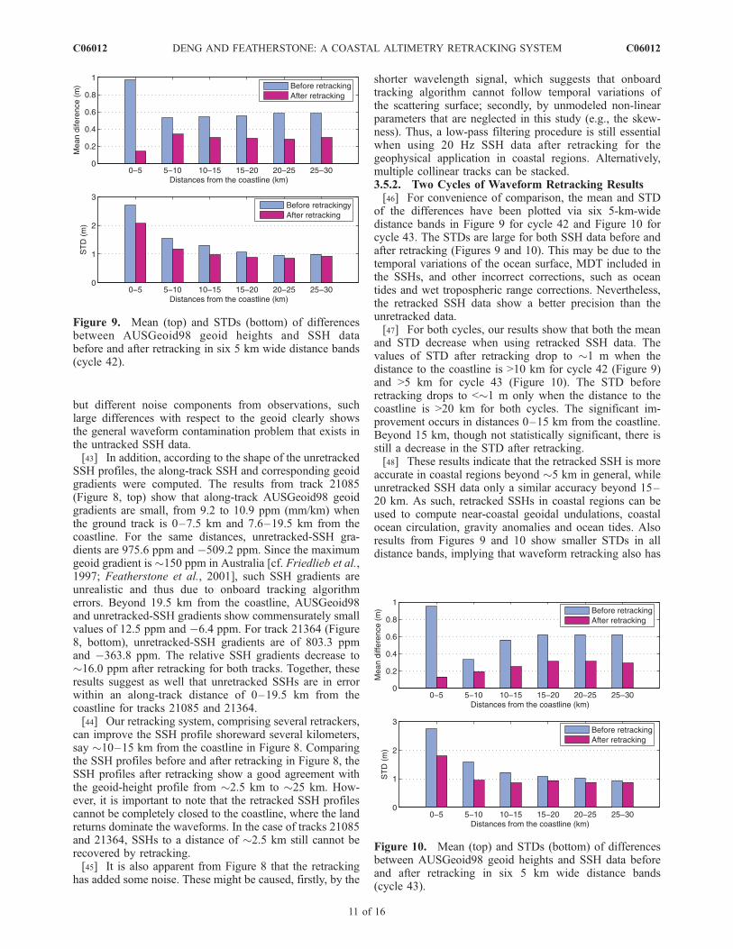
and STD decrease when using retracked SSH data. Thevalues of STD after retracking drop to �1 m when thedistance to the coastline is >10 km for cycle 42 (Figure 9)and >5 km for cycle 43 (Figure 10). The STD beforeretracking drops to <�1 m only when the distance to thecoastline is >20 km for both cycles. The significant im-provement occurs in distances 0–15 km from the coastline.Beyond 15 km, though not statistically significant, there isstill a decrease in the STD after retracking.[48] These results indicate that the retracked SSH is more
accurate in coastal regions beyond �5 km in general, whileunretracked SSH data only a similar accuracy beyond 15–20 km. As such, retracked SSHs in coastal regions can beused to compute near-coastal geoidal undulations, coastalocean circulation, gravity anomalies and ocean tides. Alsoresults from Figures 9 and 10 show smaller STDs in alldistance bands, implying that waveform retracking also has
Figure 9. Mean (top) and STDs (bottom) of differencesbetween AUSGeoid98 geoid heights and SSH databefore and after retracking in six 5 km wide distance bands(cycle 42).
Figure 10. Mean (top) and STDs (bottom) of differencesbetween AUSGeoid98 geoid heights and SSH data beforeand after retracking in six 5 km wide distance bands(cycle 43).
C06012 DENG AND FEATHERSTONE: A COASTAL ALTIMETRY RETRACKING SYSTEM
11 of 16
C06012
the potential to improve SSHs beyond 30 km from thecoastline and over open oceans.
4. Discussion and Conclusions
[49] In an effort to improve altimeter-derived SSH resultsin the well-known problematic coastal regions, this studyhas developed and tested a coastal retracking system toreprocess satellite radar altimeter waveform data for extract-ing improved SSH data sets in coastal regions. Investiga-tions of waveform characteristics demonstrate that diversewaveform shapes exist around the Australian coast, and theretracking of 20 Hz waveform data can effectively removemost errors caused by coastal sea states and land-contam-ination. The development of the coastal retracking systemincludes design and investigation of algorithms, selection ofthreshold levels, estimation of biases among differentretrackers, as well as the tests on the effectiveness of thesystem. Two cycles (43 and 44) of ERS-2 20 Hz waveformdata within 350 km from the Australian coast have beenused for implementation of the system. The AUSGeoid98model is used as a quasi-independent ground truth for someof the comparisons.[50] Selection of the threshold retracking level was per-
formed by comparing AUSGeoid98 ‘‘ground truth’’ withthe SSH data before and after threshold retracking, in ten15� � 15� sub-areas and two 5-km-wide distance bandsaround Australia. Our results confirm that the 50% thresh-old level is the best for open-ocean waveform, but is not anappropriate level for contaminated coastal waveforms. In-stead, a varying threshold level, which is drops to 30% forsome waveforms, gives a good agreement between theretracked SSH data and AusGeoid98. This value also agreeswith that used by Brooks et al. [1997].[51] Biases exit among retracked SSH data from different
retracking algorithms. Biases have been analyzed andestimated by retracking ocean waveforms using two cyclesof ERS-2 data. The bias between the SSH data retracked bythe ocean and 5-parameter fitting algorithms is 0.85 ±1.35 cm, which is not statistically significant. However, thebias between the 50%-threshold-retracked SSH data and thefitting algorithms (ocean and 5-parameter) is significant at+56.35 ± 5.84 cm, which suggest that this bias must beestimated and applied to the data to obtain consistent resultsafter retracking.[52] Our waveform classification shows that �80% of
contaminated waveforms in coastal regions present anocean-like shape, but other shapes are found much closerto the coastline from this data set (1.73–3.12 km onaverage), in particular high-peaked waveforms (1.73 kmfrom the coastline on average). The waveforms showdifferent percentages when using different retrackers as afunction of the sub-area along ground tracks. Retracking inAustralian coastal regions shows that �80%–96% of wave-forms can be retracked using a least squares iterative fittingalgorithm, while �4%–17% of waveforms have to beretracked by the threshold algorithm.[53] Of these waveforms retracked by fitting algorithms,
�98% are fitted using the ocean model (or the 5-parametermodel with a linear trailing edge) and the rest are fitted bythe 5-parameter model with an exponential trailing edge and
the 9-parameter model with either a linear trailing edge oran exponential trailing edge. This indicates that most wave-forms in Australian coastal regions are mainly dominated byreturns from a single scattering surface. It was also foundthat the need to use the threshold retracker decreases withincreasing offshore distance (35% of waveforms within 0–5km to 4% of waveforms within 5–10 km). Beyond 10 km,only 2% of waveforms are threshold retracked, indicatingthat the method developed to categorize coastal waveformsis effective.[54] When comparing AUSGeoid98 with SSH data in
Australian coastal regions, single-track comparisons show thatthe SSH gradients in the vicinity of the land before retrackingare large, varying from �363.8–�975.6 mm/km overalong-track distances of 4.7–19.5 km, which is much largerthan the maximum geoid gradient value of �150 mm/km inAustralia. After retracking, the SSH gradients decrease by�16.0 mm/km, agreeing well with the geoid gradient over thesame distance. This quasi-independent validation, thoughignoring DMT, strongly indicates that retracking improvesthe altimeter-derived SSH in coastal regions.[55] In general, our coastal waveform retracking system
has substantially improved and extended altimeter-derivedSSHs �10–15 km shoreward in Australian coastal regionscompared with unretracked SSH data, using AUSGeoid98as a quasi-independent reference. As such, the altimeter-derived SSH profiles are now believed to be more accuratebeyond �5 km from the Australian coastline.[56] These improved SSHs also show the same precision
as those over open oceans, thus indicating a great potentialto apply them to geodetic applications (e.g., tide determi-nation) in coastal regions. However, SSH profiles 0–2.5 kmfrom the coastline still cannot be recovered by the wave-form retracking procedure at the same level of precision.This is attributed to a combination of severe contaminationfrom land and inland water returns, the rougher sea states, aswell as incorrect geophysical corrections in these near landareas.[57] The improvement of the altimeter SSH in Australian
coastal waters has demonstrated that our coastal waveformretracking system has the potential to be applied to othercoastal regions, as well as to other satellite altimeterwaveform data sets (e.g., Jason-1, Envisat and GFO).Higher accuracy of altimeter measurements in coastalregions will help realize a more complete coverage ofaltimetry missions for various scientific studies.
Appendix A: Algorithms Used in the CoastalWaveform Retracking System
A1. Ocean Model
[58] Following Brown [1977], the time series of the meanreturned power waveform P(t) measured by a satellitealtimeter is analytically expressed in the time domain as[e.g., Hayne, 1980; Rodriguez, 1988; Rodriguez andChapman, 1989; Amarouche et al., 2004]
P tð Þ ¼ PN þ 1
2A erf
tffiffiffi2
p� �
þ 1
� exp d tþ d
2
� �� ðA1Þ
C06012 DENG AND FEATHERSTONE: A COASTAL ALTIMETRY RETRACKING SYSTEM
12 of 16
C06012
where A is an amplitude scaling term, PN is the altimeter’sthermal noise, and
t ¼ t t0
s d ðA2Þ
d ¼ a b2
4
� �s ðA3Þ
where t is the time measured at the satellite such that t = t0corresponds to the range to the instantaneous sea level(averaged over the footprint) at nadir, s is the waveformrise-time (i.e., the information relative to the sea surfaceroughness through the SWH), and
a ¼ 4c
gh
1
1þ h=Rð Þ cos 2xð Þ ðA4Þ
b ¼ 4
g
c
h
1
1þ h=Rð Þ
� �1=2
sin 2xð Þ ðA5Þ
where R � 6371005 m is the spherical radius of the Earth[Moritz, 1980], h is the satellite altitude above the referenceellipsoid, g is a function of the antenna beam-widthparameter q defined by Brown [1977], and x is the off-nadir angle.[59] The retracking process estimates five parameters of
PN, A, t0, s and x. These estimates are performed makingthe measured waveform coincide with equation (A1)according to the iterative least squares fitting procedure.
A2. Threshold Retracking
[60] The empirical method of threshold retracking isbased upon the dimensions of a rectangle about the ampli-tude (A), width (W), and center of gravity (COG) definedand computed using the off-center of gravity (OCOG)retracking method [e.g., Wingham et al., 1986; Partingtonet al., 1991; Davis, 1995]. The OCOG defines that the areaof the rectangle equals that of the waveform, and the heightof the COG is a half of the amplitude of the waveform. Toreduce the effect of low-amplitude samples in front of theleading edge, the squares of the sample values are used inthe computation. The equations used to compute A, W andCOG are given in Deng et al. [2002].[61] The threshold value is then referenced to the ampli-
tude [e.g., Bamber, 1994] or the maximum waveformsample [e.g., Zwally et al., 1990; Davis, 1997] estimate ofthe rectangle at 25%, 50%, or 75% of the waveformamplitude. The selection of an optimum threshold level iscritical, because the range is determined from it. Theretracking gate estimate is determined by linearly interpo-lating between adjacent samples of a threshold crossing atsteep part of the leading edge of the waveform. Thisalgorithm maintains the same advantages as the OCOG,but it can determine a more accurate tracking gate positionthan the OCOG [Partington et al., 1991]. A disadvantage isthat, like the OCOG method, it is not based on a physicalmodel.
A3. B-Parameter Retracking
[62] Martin et al. [1983] develope the first retrackingalgorithm for processing altimeter return waveforms overcontinental ice sheets. This algorithm fits a 5- or 9-param-eter function to the waveform reflected from one or twoscattering surfaces over ice sheets. It is also known as b-parameter retracking or the NASA algorithm [e.g., Davis,1995]. The general function fitting the radar returns is[Martin et al., 1983; Zwally et al., 1990]:
y tð Þ ¼ b1 þXni¼1
b2i 1þ b5iQið ÞP t b3ib4i
� �ðA6Þ
where
Qi ¼0 for t < b3i þ 0:5b4i
t b3i þ 0:5b4ið Þ for t b3i þ 0:5b4i
8<: ðA7Þ
P xð Þ ¼Z x
1
1ffiffiffiffiffiffi2p
p expq2
2
� �dq ðA8Þ
where n = 1 or 2 is the number of the ramp in the waveformthat corresponds to single- or double-reflecting surfaces,respectively. Double ramps indicate that two distinct, nearlyequidistant surfaces are tracked. The unknown parametersare the thermal noise level b1, amplitude b2i, mid-point(s) onthe leading edge of the waveform b3i, the waveform rise-time b4i, and the slope of the trailing edge b5i. When i = 1 inequation (A6), the corresponding function is 5-parametermodel.[63] When the linear trailing edge is replaced by an
exponential decay term [cf. Zwally et al., 1990], equation(A6) is adapted to give
y tð Þ ¼ b1 þXni¼1
b2i exp b5iQið ÞP t b3ib4i
� �ðA9Þ
where
Qi ¼0 for t < b3i 2b4i
t b3i þ 0:5b4ið Þ for t b3i 2b4i
8<: ðA10Þ
This function can be used to fit the waveform with a fast-decaying trailing edge, which is caused by beamattenuation. It simulates the antennae attenuation as thepulse expands on the surface beyond the pulse-limitedfootprint.
Appendix B: Comparison Between Oceanand 5-Parameter Models
[64] Both the ocean (equation (A1)) and 5-parametermodels (equations (A6) and (A9)) are based upon the Brown[1977] model. Comparison between them will give qualita-tive guidance to selecting an adequate fitting function forcoastal retracking. In the trailing edge, the normal proba-bility distribution P(x) (or the erf function) is equal to unity
C06012 DENG AND FEATHERSTONE: A COASTAL ALTIMETRY RETRACKING SYSTEM
13 of 16
C06012
for SWHs < 10 m. Thus, in this region, equations (A1),(A6), and (A9) can be written as Pt(t), yt(t), and yte(t)
ln Pt tð Þ PNð Þ ¼ ln Að Þ þ d
st0
d2
2
� d
st ðB1Þ
yt tð Þ ¼ b1 þ b21 1þ b51Q1ð Þ ðB2Þ
and
ln yte tð Þ be1ð Þ ¼ ln be21ð Þ be51Q1 ðB3Þ
where d/s, b51 and be51 are the slope of the waveformtrailing edge related to fitting functions.[65] According to equation (A3), the slope (d/s) of the
trailing edge in the ocean model is related to the physical
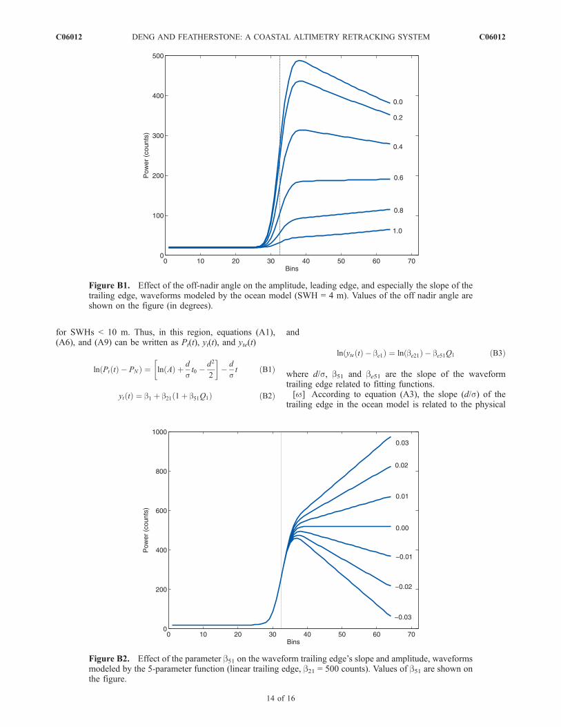
Figure B1. Effect of the off-nadir angle on the amplitude, leading edge, and especially the slope of thetrailing edge, waveforms modeled by the ocean model (SWH = 4 m). Values of the off nadir angle areshown on the figure (in degrees).
Figure B2. Effect of the parameter b51 on the waveform trailing edge’s slope and amplitude, waveformsmodeled by the 5-parameter function (linear trailing edge, b21 = 500 counts). Values of b51 are shown onthe figure.
C06012 DENG AND FEATHERSTONE: A COASTAL ALTIMETRY RETRACKING SYSTEM
14 of 16
C06012
parameters of the antenna gain pattern, the Earth’s radiusand the off-nadir angle x. Of these parameters, x is impor-tant because it affects the slope of the trailing edge(Figure B1). From Figure B1, x changes not only the slopeof the trailing edge, but also the slope of the leading edge.The slope of the leading edge decreases with increasing x,while the slope of the trailing edge increases with increasingx. However, the location (or range to the instantaneous seasurface averaged over the footprint) of the mid-point on theleading edge does not change with varying x.[66] The amplitude of the waveform is also affected
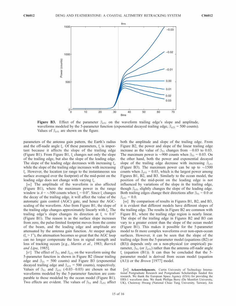
(Figure B1), where the maximum power in the rangewindow is A = �500 counts when x = 0.0�. Since x changesthe decay of the trailing edge, it will affect the value of theautomatic gain control (AGC) gate, and hence the AGC-scaling of the waveform. Also from Figure B1, the slope ofthe trailing edge changes approximately linearly with x. Thetrailing edge’s slope changes its direction at x � 0.6�(Figure B1). The reason is as the surface slope increasesfrom zero, the pulse-limited footprint moves from the centreof the beam, and the leading edge and amplitude areattenuated by the antenna gain function. At steeper angles(x > 1�), the attenuation becomes so great that the AGC loopcan no longer compensate the loss in signal strength andloss of tracking occurs [e.g., Martin et al., 1983; Barrickand Lipa, 1985].[67] The effect of b51 and be51 on the waveform using the
5-parameter function is shown in Figure B2 (linear trailingedge and b21 = 500 counts) and Figure B3 (exponentialdecayed trailing edge and be21 = 500 counts), respectively.Values of b51 and be51 (-0.03–0.03) are chosen so thatwaveforms modeled by the 5-parameter function are com-parable to those modeled by the ocean model (Figure B1).Two effects are evident. The values of b51 and be51 affect
both the amplitude and slope of the trailing edge. FromFigure B2, the power and slope of the linear trailing edgeincrease as the value of b51 changes from 0.03 to 0.03.The maximum power is �900 counts when b51 = 0.03. Onthe other hand, both the power and exponential decayedslope of the trailing edge decrease with increasing be51(Figure B3). The maximum power can be up to �1500counts when be51 = 0.03, which is the largest power amongFigures B1, B2, and B3. Similarly to the ocean model, theposition of the mid-point on the leading edge is notinfluenced by variations of the slope in the trailing edge,though be51 slightly changes the slope of the leading edge.Both trailing edges change their directions after b51 = 0.0 orbe51 = 0.0.[68] By comparison of results in Figures B1, B2, and B3,
it is evident that different models have different slopes ofthe trailing edge. The results in Figure B2 are common withFigure B1, where the trailing edge region is nearly linear.The slope of the trailing edge in Figures B2 and B3 canvary to a greater extent than the slope of the ocean model(Figure B1). This makes it possible for the 5-parametermodel to fit more complex waveforms over non-open-oceansurfaces. However, it can be seen that the slope of thetrailing edge from the 5-parameter model (equations (B2) or(B3)) depends only on a non-physical (or empirical) pa-rameter, b51 (or be51) rather than the antenna off-nadir anglex (equation (B1)). It can thus be concluded that the 5-parameter model is derived from ocean model (equation(A1)) or the Brown [1977] model.
[69] Acknowledgments. Curtin University of Technology Interna-tional Postgraduate Research and Postgraduate Scholarships funded thisresearch. We thank the European Space Agency (ESA) for providing theERS-1 waveform data. We thank Phillipa Berry (De Montfort University,UK), Cheinway Hwang (National Chiao Tung University, Taiwan), Jon
Figure B3. Effect of the parameter be51 on the waveform trailing edge’s slope and amplitude,waveforms modeled by the 5-parameter function (exponential decayed trailing edge, be21 = 500 counts).Values of be51 are shown on the figure.
C06012 DENG AND FEATHERSTONE: A COASTAL ALTIMETRY RETRACKING SYSTEM
15 of 16
C06012
Kirby (Curtin University of Technology, Australia), Graham Quartly(Southampton Oceanography Centre, UK), O.P. Knudsen and O.B. Ander-sen (Danish National Space Centre, Demark), J.D. Fairhead (University ofLeeds, UK), Ronald Brooks (NASA, USA) and George Hayne (NASA,USA) for providing some references and numerous useful discussions. Wealso thank the anonymous reviewers and the editor (James Kirby) for theircomments on this manuscript.
ReferencesAmarouche, L., P. Thibaut, O. Z. Zanife, J.-P. Dumont, P. Vincent, andN. Steunou (2004), Improving the Jason-1 ground retracking to betteraccount for attitude effects, Mar. Geod., 27, 171–197.
Andersen, O. B., and P. Knudsen (2000), The role of satellite altimetry ingravity field modelling in coastal areas, Phys. Chem. Earth A, 25(1), 17–24.
Anzenhofer, M., C. K. Shum, and M. Renstch (2000), Coastal altimetry andapplications, report, Ohio State Univ., Columbus.
Bamber, J. L. (1994), A digital elevation model of the Antarctic ice sheetderived from ERS-1 altimeter data and comparison with terrestrial mea-surements, Ann. Glaciol., 20, 48–54.
Barrick, D. E., and B. J. Lipa (1985), Analysis and interpretation of alti-meter sea echo, Adv. Geophys., 27, 61–100.
Brenner, A. C., C. J. Koblinsky, and H. J. Zwally (1993), Postprocessingof satellite return signals for improved sea surface topography accuracy,J. Geophys. Res., 98(C1), 933–944.
Brooks, R. L., D. W. Lockwood, and J. E. Lee (1997), Land effects onTOPEX radar altimeter measurements on Pacific Rim coastal zones,NASA WFF Publ. (Available at http://topex.wff.nasa.gov/)
Brown, G. S. (1977), The average impulse response of a rough surface andits applications, IEEE Trans. Antennas Propag., 25(1), 67–74.
Buchanan, C. (1991), Bathymetric 30 arc second grid of the Australianregion [CD-ROM], Geosci. Aust., Canberra, Australia.
Chelton, D. B., J. C. Ries, B. J. Haines, L.-L. Fu, and P. S. Callahan (2001),Satellite altimetry, in Satellite Altimetry and Earth Sciences: A Handbookof Techniques and Applications, edited by L.-L. Fu and A. Cazenave, pp.1–132, Elsevier, New York.
Davis, C. H. (1995), Growth of the Greenland Ice Sheet: A performanceassessment of altimeter retracking algorithms, IEEE Trans. Geosci. Re-mote Sens., 33(5), 1108–1116.
Davis, C. H. (1997), A robust threshold retracking algorithm for measuringice-sheet surface elevation change from satellite radar altimeter, IEEETrans. Geosci. Remote Sens., 35(4), 974–979.
Deng, X. (2004), Improvement of geodetic parameter estimation in coastalregions from satellite radar altimetry, Ph.D. thesis, 248 pp., Curtin Univ.of Technol., Perth, Australia.
Deng, X., W. E. Featherstone, C. Hwang, and P. A. M. Berry (2002),Estimation of contamination of ERS-2 and POSEIDON satellite radaraltimetry close to the coasts of Australia, Mar. Geod., 25(4), 249–271.
Dong, X., P. Moore, and R. Bingley (2002), Absolute calibration of theTOPEX/POSEIDON altimeter using UK tide gauges, GPS, and preciselocal geoid-differences, Mar. Geod., 25, 189–204.
Dunbar, P. (2000), DS759.2 – Terrain base, global 5-minute ocean depthand land elevation, Natl. Geophys. Data Cent., Boulder, Colo. (Availableat http://dss.ucar.edu/datasets/ds759.2/)
Fairhead, J. D., C. M. Green, and M. E. Odegard (2001), Satellite-derivedgravity having an impact on marine exploration, The Leading Edge, 20,873–876.
Featherstone, W. E., J. F. Kirby, A. H. W. Kearsley, J. R. Gilliland, G. M.Johnston, J. Steed, R. Forsberg, and M. G. Sideris (2001), TheAUSGeoid98 geoid model of Australia: data treatment, computationsand comparisons with GPS-levelling data, J. Geod., 75, 13–330.
Fernandes, M. J., L. Bastos, and M. Antunes (2003), Coastal satellite alti-metry - methods for data recovery and validation, in Gravity and Geoid2002, edited by I. N. Tziavos, pp. 302–307, Dep. of Surv. and Geod.,Aristotle Univ. of Thessaloniki, Thessaloniki.
Friedlieb, O. J., W. E. Featherstone, and M. C. Dentith (1997), A WGS84-AHD profile over the darling fault, Western Australia, Geomatics Res.Australasia, 67, 17–32.
Hayne, G. S. (1980), Radar altimeter mean return waveform from near-normal-incidence ocean surface scattering, IEEE Trans. Antennas Pro-pag., 28(5), 687–692.
Hayne, G. S., and D. W. Hancock III (1990), Corrections for the effects ofsignificant wave height and attitude on Geosat radar altimeter measure-ments, J. Geophys. Res., 95(C3), 2837–2842.
Levitus, S. (1982), Climatological atlas of the World Ocean, Natl. OceanicAtmos. Admin., Prof. Pap., 13, 1–180.
Li, D. R. (1988), The Error and Reliability Theory, 331 pp., Surv. andMapp., Beijing, China.
Mantripp, D. (1996), Radar altimetry, in The Determination of GeophysicalParameters From Space, edited by N. E. Fancey, I. D. Gardiner, and R. A.Gardiner, pp. 119–171, Inst. of Phys., London, UK.
Martin, T. V., H. J. Zwally, A. C. Brenner, and R. A. Bindschadler (1983),Analysis and retracking of continental ice sheet radar altimeter wave-forms, J. Geophys. Res., 88(C3), 1608–1616.
Moritz, R. S. (1980), Advanced Physical Geodesy, 500 pp., Wichmann,Karlsruhe.
Nerem, R. S. (1995), Measuring global mean sea level variations usingTOPEX/POSEIDON altimeter data, J. Geophys. Res., 100(C12),25,135–25,151.
NRSC (1995), Altimeter waveform product alt.wap compact user guide,PF-UG-NRL-AL-0001, 32 pp., U.K. Process. and Arch. Facil., UK.
Partington, K. C., W. Cudlip, and C. G. Rapley (1991), An assessment ofthe capability of the satellite radar altimeter for measuring ice sheettopographic change, Int. J. Remote Sens., 12(3), 585–609.
Quartly, G. D., and M. A. Srokosz (2001), Analyzing altimeter artifacts:statistical properties of ocean waveforms, J. Atmos. Oceanic Technol., 18,2074–2091.
Rodriguez, E. (1988), Altimetry for non-Gaussian oceans: height biases andestimation of parameters, J. Geophys. Res., 93(C11), 14,107–14,120.
Rodriguez, E., and B. Chapman (1989), Exacting ocean surface informationfrom altimeter returns: the deconvolution method, J. Geophys. Res.,94(C7), 9761–9778.
Strub, P. L., and C. James (1997), Satellite comparisons of eastern boundarycurrents: resolution features in ‘‘coastal’’ oceans, paper presented at Mon-itoring the Oceans in the 2000s: An Integrated Approach, Biarritz,France.
Thom, B. G. (1984), Geomorphic research on the coast of Australia: Apreview, in Coastal Geomorphology in Australia, edited by B. G. Thom,pp. 1–15, Elsevier, New York.
Wang, Y.-M., and R. H. Rapp (1991), Geoid gradients for Geosat andTopex/Poseidon repeat ground tracks, Rep. 408, 26 pp., Ohio State Univ.,Columbus.
Wessel, P., and W. H. F. Smith (1996), A global, self-consistent, hierarch-ical, high-resolution shoreline database, J. Geophys. Res., 101(B4),8741–8743.
Wingham, D. J., C. G. Rapley, and H. Griffiths (1986), New techniques insatellite tracking systems, in Proceedings of IGARSS’ 88 Symposium,Zurich, Switzerland, September, pp. 1339–1344, IEEE Press, Piscat-away, N. J.
Zwally, H. J., A. C. Brenner, J. A. Major, and R. A. Bindschadler (1990),Satellite radar altimetry over ice, volumes 1, 2, and 4, NASA Ref. Publ.,1233.
X. Deng, Discipline of Civil, Surveying and Environmental Engineering,
University of Newcastle, University Drive, Callaghan, NSW 2308,Australia. ([email protected])W. E. Featherstone, Western Australian Centre for Geodesy, Curtin
University of Technology, GPO Box U1987, Perth, WA 6845, Australia.
C06012 DENG AND FEATHERSTONE: A COASTAL ALTIMETRY RETRACKING SYSTEM
16 of 16
C06012