A closer look at the hysteresis loop for ferromagnets - A survey of misconceptions and misinterpretations in textbooks

Hilda W. F. Sung and Czeslaw Rudowicz

Department of Physics and Materials Science, City University of Hong Kong, 83 Tat Chee Avenue,

Kowloon, Hong Kong SAR, People�s Republic of China

This article describes various misconceptions and misinterpretations concerning presentation

of the hysteresis loop for ferromagnets occurring in undergraduate textbooks. These problems

originate from our teaching a solid state / condensed matter physics (SSP/CMP) course. A closer

look at the definition of the 'coercivity' reveals two distinct notions referred to the hysteresis

loop: B vs H or M vs H, which can be easily confused and, in fact, are confused in several

textbooks. The properties of the M vs H type hysteresis loop are often ascribed to the B vs H

type loops, giving rise to various misconceptions. An extensive survey of textbooks at first in the

SSP/CMP area and later extended into the areas of general physics, materials science and

magnetism / electromagnetism has been carried out. Relevant encyclopedias and physics

dictionaries have also been consulted. The survey has revealed various other substantial

misconceptions and/or misinterpretations than those originally identified in the SSP/CMP area.

The results are presented here to help clarifying the misconceptions and misinterpretations in

question. The physics education aspects arising from the textbook survey are also discussed.

Additionally, analysis of the CMP examination results concerning questions pertinent for the

hysteresis loop is provided.

Keywords: ferromagnetic materials; hysteresis loop; coercivity; remanence; saturation induction

1. Introduction

During years of teaching the solid state physics

(SSP), which more recently become the condensed

matter physics (CMP) course, one of us (CZR),

prompted by questions from curious students

(among others, HWFS), has realized that textbooks

contain often not only common misprints but

sometimes more serious misconceptions. The latter

occur mostly when the authors attempt to present a

more advanced topic in a simpler way using

schematic diagrams. One such case concerns

presentation of the magnetic hysteresis loop for

ferromagnetic materials. Having identified some

misconceptions existing in several textbooks

currently being used for our SSP/CMP course at

CityU, we have embarked on an extensive literature

survey. Search of physics education journals have

revealed only a few articles dealing with magnetism,

e.g. Hickey & Schibeci (1999), Hoon & Tanner

(1985). Interestingly, a review of middle school

physical science texts by Hubisz (http://www.psrc-

online.org/curriculum/book.html), which has

recently come to our attention, provides ample

1

examples of various errors and misconceptions

together with pertinent critical comments. However,

none of these sources have provided clarifications of

the problems in question. To find out the extent of

these misconceptions existing in other physics areas,

we have surveyed a large number of available

textbooks pertinent for solid state / condensed

matter, general physics, materials science, and

magnetism / electromagnetism. Several pertinent

encyclopedias and physics dictionaries have also

been consulted. The survey has given us more than

we bargained for, namely, it has revealed various

other substantial misconceptions than those

originally identified in the SSP/CMP area. The

results of this survey are presented here for the

benefit of physics teachers (as well as researchers)

and students. The textbooks, in which no relevant

misconceptions and/or confusions were identified,

are not quoted in text, however, they are listed for

completeness in Appendix I in order to provide a

comprehensive information on the scope of our

survey.

In order to provide the counterexamples for the

misconceptions identified in the textbooks, we have

reviewed a sample of recent scientific journals

searching for real examples of the magnetic

hysteresis loop, beyond the schematic diagrams

found in most textbooks. To our surprise a number

of general misconceptions concerning magnetism

have been identified in this review. The results of

this review are presented in a separate article, which

focuses on the research aspects and provides recent

literature data on soft and hard magnetic materials

(Sung & Rudowicz, 2002; hereafter referred to as S

& R, 2002).

The root of the problem appears to be the

existence of two ways of presenting the hysteresis

loop for ferromagnets: (i) B vs H curve or (ii) M vs

H curve. In both cases, the �coercivity� (�coercive

force�) is defined as the point on the negative H-

axis, often using an identical symbol, most

commonly Hc. Yet it turns out that the two

meanings of �coercivity� are not equivalent. In some

textbooks the second notion of coercivity (M vs H)

is distinguished from the first one (B vs H) as the

�intrinsic� coercivity Hci. An apparent identification

of the two meanings of coercivity Hc (B vs H) and

Hci (M vs H) as well as of the properties of soft and

hard magnetic materials have lead to

misinterpretation of Hc as the point on the B vs H

hysteresis loop where the magnetization is zero.

This is evident, for example, in the statements

referring to Hc as the point at which �the sample is

again unmagnetized� (Serway, 1990) or �the field

required to demagnetize the sample� (Rogalski &

Palmer, 2000). Other misconceptions identified in

our textbook survey concern: 'saturation induction

Bsat� and the inclination of the B vs H curve after

saturation, shape of the hysteresis loop for soft

magnetic materials, and presentation of the

hysteresis loop for both soft and hard ferromagnets

in the same diagram. Minor problems concerning

terminology and the drawbacks of using schematic

diagrams are also discussed. Analysis of the

condensed matter physics examination results

concerning questions pertinent for the hysteresis

loop is provided to illustrate some popular

misconceptions in students' understanding.

2. Two notions of coercivity

For a ferromagnetic material, the magnetic

induction (or the magnetic field intensity) inside the

2

sample, B, is defined as (see, e.g. any of the books

listed in References):

B = H + 4πM (CGS);

B = µo ( H + M ) (SI) (1)

where M is the magnetization induced inside the

sample by the applied magnetic field H. In the free

space: M = 0 and then in the SI units: B ≡ µo H,

where µo is the permeability of free space (µo = 4π x

10-7 [m kg A-2 sec-2]; note that the units [Hm-1] and

[WbA-1m-1] are also in use). The standard SI units

are: B [tesla] = [T], H and M [A/m], whereas B

[Gauss] = [G], H [Oersted] = [Oe], and M [emu/cc]

(see, e.g. Jiles, 1991; Anderson, 1989). Both the

CGS units and the SI units are provided since the

CGS unit system is in use in some textbooks

surveyed and comparisons of values need to be

made later.

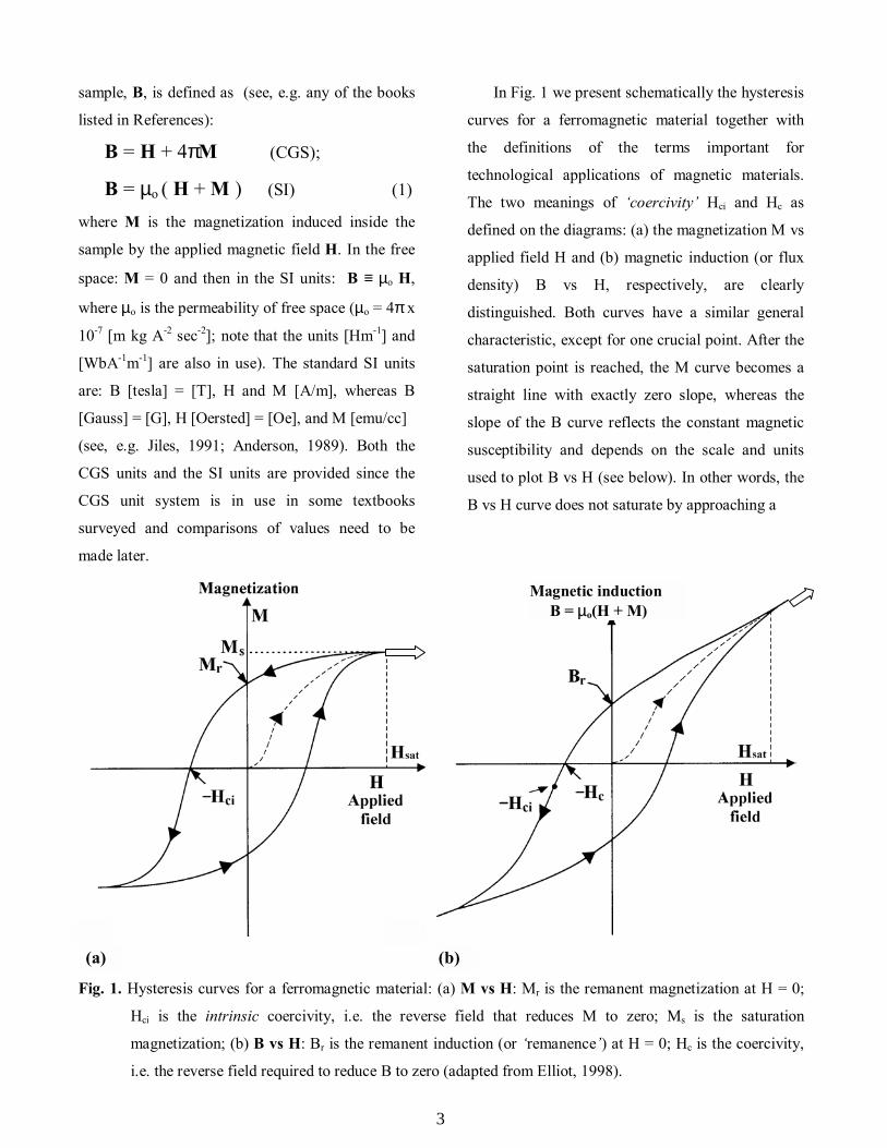
In Fig. 1 we present schematically the hysteresis

curves for a ferromagnetic material together with

the definitions of the terms important for

technological applications of magnetic materials.

The two meanings of �coercivity� Hci and Hc as

defined on the diagrams: (a) the magnetization M vs

applied field H and (b) magnetic induction (or flux

density) B vs H, respectively, are clearly

distinguished. Both curves have a similar general

characteristic, except for one crucial point. After the

saturation point is reached, the M curve becomes a

straight line with exactly zero slope, whereas the

slope of the B curve reflects the constant magnetic

susceptibility and depends on the scale and units

used to plot B vs H (see below). In other words, the

B vs H curve does not saturate by approaching a

Fig. 1. Hysteresis curves for a ferromagnetic material: (a) M vs H: Mr is the remanent magnetization at H = 0;

Hci is the intrinsic coercivity, i.e. the reverse field that reduces M to zero; Ms is the saturation

magnetization; (b) B vs H: Br is the remanent induction (or �remanence�) at H = 0; Hc is the coercivity,

i.e. the reverse field required to reduce B to zero (adapted from Elliot, 1998).

Magnetic induction B = µo(H + M)

(b) (a)

3

limiting value as in the case of the M vs H curve.

For an initially unmagnetized sample, i.e. M ≡ 0

at H = 0, as H increases from zero, M and B

increases as shown by the dashed curves in Fig. 1

(a) and (b), respectively. This magnetization process

is due to the motion and growth of the magnetic

domains, i.e. the areas with the same direction of

the local magnetization. For a full discussion of the

formation of hysteresis loop and the nature of

magnetic domains inside a ferromagnetic sample

one may refer to the specialized textbooks listed in

the References, e.g. Kittel (1996), Elliott (1998),

Dalven (1990), Skomski & Coey (1999). Here we

provide only a brief description of these aspects. A

distinction must be made at this point between the

magnetically isotropic materials, for which the

magnetization process does not depend on the

orientation of the sample in the applied field H, and

the anisotropic ones, which are magnetized first in

the easy direction at the lower values of H. In the

former case, as each domain magnetization tends

to rotate to the direction of the applied field Kittel

(1996), the domain wall displacements occur,

resulting in the growth of the volume of domains

favorably oriented (i.e. parallel) to the applied field

and the decrease of the unfavorably oriented

domains Kittel (1996). In the latter case, only after

the magnetic anisotropy (for definition, see, e.g.

Kittel (1996), Elliott (1998), Dalven (1990),

Skomski & Coey (1999), Jiles (1991)) is overcome

the sample is fully magnetized with the direction of

M along H. In either case, when this �saturation

point� is reached, the magnetization curve no longer

retraces the original dashed curve when H is

reduced. This is due to the irreversibility of the

domain wall displacements. When the applied field

H reaches again zero, the sample still retains some

magnetization due to the existence of domains still

aligned in the original direction of the applied field

Dalven (1990). The respective values at H = 0 are

defined (see, e.g. Kittel (1996), Elliott (1998),

Dalven (1990), Skomski & Coey (1999), Jiles

(1991)) as the remnant magnetization Mr, Fig. 1

(a), and the remnant induction Br, Fig. 1 (b). To

reduce the magnetization M and magnetic induction

B to zero, a reverse field is required known as the

coercive force or coercivity. The soft and hard

magnetic materials are distinguished by their small

and large area of the hysteresis loop, respectively.

By definition, the coercive force (coercivity)

defined in Fig. 1 (a), and that in Fig. 1 (b) are two

different notions, although their values may be very

close for some materials. In order to distinguish

them, some authors define either the related

coercivity (Kittel, 1996) or the intrinsic coercivity

(Elliott, 1998; Jiles, 1991) Hci as the reverse field

required to reduce the magnetization M from the

remnant magnetization Mr again to zero as shown in

Fig. 1 (a), whereas reserve the symbol Hc and the

name coercivity (coercive force) to denote the

reverse field required to reduce the magnetic

induction in the sample B to zero as shown in Fig. 1

(b), as done, e.g. by Kittel (1996). Hence, the

confusion between the two notions of coercivity

referred to the curve B vs H and the curve M vs H

can be avoided. Since a clear distinction between Hc

and Hci, is often not the case in a number of

textbooks, a question arises under what conditions

and for which magnetic systems, if any, Hc and Hci

can be considered as equivalent quantities. If it was

the case, the point �Hc on the B vs H curve would

also correspond to the magnetization M ≡ 0 as in the

4

case of Hci on the M vs H curve. Only in one of the

books surveyed such approximation is explicitly

considered. Dalven (1990) shows that, in general,

the values of B and M are much larger than H in

both curves in Fig. 1. Hence, if H can be neglected

in Eq. 1, then B ≈ µoM. This turns to be valid only

for low values of H and the narrow hysteresis loop

pertinent for the soft magnetic materials. In other

words, the value of Hc and Hci are indeed very

close, so not identical, for the soft magnetic

materials only. In this case Hci in Fig. 1 (a) and

Hc in Fig. 1 (b) can be considered as two equivalent

points and hence M ≈ 0 at Hc as well.

The real examples of the magnetic hysteresis

loop, identified in our review (S & R, 2002) of a

sample of recent scientific journals, indicate that Hc

and Hci turn out to be significantly non-equivalent

for the hard magnetic materials. In the article (S &

R, 2002) we have also complied values of Hci, Hc,

and Br for several commercially available

permanent magnetic materials revealed by our

recent Internet search. These data indicate that

although Hc and Hci are of the same order of

magnitude, in a number of cases Hci is substantially

larger than Hc. Hence, in general, it is necessary to

distinguish between Hc and Hci. Moreover, as a

consequence of Hci ≠ Hc, the magnetization does not

reach zero at the point �Hc on the B vs H curve but

at a larger value of Hci indicated schematically in

Fig. 1 (b). However, in the early investigations of

magnetic materials, before the present day very

strong permanent magnets become available, the

values of Hc and Hci were in most cases not

distinguishable. As the advances in the magnet

technology progressed, more and more hard

magnetic materials have been developed, for which

the distinction between Hci and Hc is quite

pronounced (see Table 1 in S & R (2002)). The

presentation in most textbooks reflects the time lag

it takes for new materials or ideas to filter from

scientific journals into the textbooks as

'schematically presented established knowledge'.

3. Results of textbooks survey

In our survey of the presentation of the

hysteresis loop for ferromagnetic materials, in total

about 300 textbooks in the area of solid state /

condensed matter, general physics, materials

science, magnetism / electromagnetism as well as

several encyclopedias and physics dictionaries

available in City University library were examined.

We have identified around 130 books dealing with

the hysteresis loop. In order to save the space an

additional list of the books surveyed (37 items),

which deal with the hysteresis loop in a correct way

but are not quoted in the References, is available

from the authors upon request.

It appears that from the points of view under

investigation, generally, the encyclopedias and

physics dictionaries contain no explicit

misconceptions. This is mainly due to the fact that

the hysteresis loop is usually presented at a rather

low level of sophistication (see, e.g. Lapedes

(1978), Lord (1986), Meyers (1990), BesanHon

(1985), Parker (1993)). However, in a few instances

in the same source book both types of hysteresis

loop (B vs H and M vs H) are discussed in separate

articles written by different authors without

clarifying the distinct notions, which may also lead

to confusion. Examples include, e.g. (a) Anderson

& Blotzer (1999) and Vermariën et al (1999), and

(b) Arrott (1983), Donoho (1983), and Rhyne

(1983). Hence, these authoritative sources could not

5

help us to clarify the intricacies we have

encountered. This have been achieved by consulting

more advanced books on the topic, e.g., Kittel

(1996), Dalven (1990), Skomski and Coey (1999),

and/or regular scientific journals (for references,

see, S & R, 2002).

Only a small number of books surveyed contain

both types of the curves: B vs H and M vs H as well

as provide clarification of the terminology

concerning Hc and Hci - Kittel (1996), Elliott (1998),

Dalven (1990), Skomski & Coey (1999), Jiles

(1991), Arrott (1983), Donoho (1983), Rhyne

(1983), Levy (1968), Anderson & Blotzer (1999),

Vermariën et al. (1999). Barger & Olsson (1987)

provide both graphs but terminology is only referred

to the B vs H graph. Most books deal only with one

type of the hysteresis loop. The B vs H curve,

which is more prone to misinterpretations, has been

used more often in the surveyed books in all areas.

A few books deal with the M vs H curve and

provide, with a few exceptions (see Section C

below), correct description and graphs (see, e.g.

Lovell et al , 1981; Aharoni, 1996; Wert &

Thomson, 1970; Elwell & Pointon, 1979). On the

other hand, the M vs H curve is dominant in

research papers surveyed (S & R, 2002).

Surprisingly, while most of the textbooks surveyed

attempt to adhere to the SI units, all but a few

research articles reviewed still use the CGS units.

This in itself is a worrying factor (S & R, 2002).

The various misconceptions and/or

misinterpretations identified in the course of our

comprehensive survey of textbooks can be classified

into five categories. Below we provide a systematic

review of the books with respect to the problems in

each category.

A. Misinterpretation of the coercivity Hc on the B

vs H curve as the point at which M=0.

This was the original problem which has

triggered the textbook survey. Various examples of

this misinterpretation, consisting in ascribing �zero

magnetization� to the point �Hc on the B vs H

hysteresis loop, are listed below with the nature of

the problem indicated by the pertinent sentences

quoted.

Solid state / condensed matter physics books

• �The magnetic field has to be reversed and

raised to a value Hc (called the coercive

force) in order to push domain walls over the

barriers so that we regain zero

magnetization.� (Wilson, 1979)

• �The point at which B=0 is the coercive field

and is usually designated as Hc. It represents

the magnetic field required to demagnetize the

specimen.� (Pollock, 1990)

• �The reverse field required to demagnetize

the material is called the coercive force, Hc.�

(Pollock, 1985)

• �To remove all magnetization from a

specimen then requires the application of a

field in the opposite direction termed the

coercive field.� (Elliott & Gibson, 1978)

• �H at c is called the coercive force and is a

measure of the field required to demagnetize

the sample.� (Rogalski & Palmer, 2000)

General physics books

• �The coercive force is a measure of the

magnitude of the external field in the opposite

6

direction needed to reduce the residual

magnetization to zero.� (Ouseph, 1986)

• �In order to demagnetize the rod completely,

H must be reversed in direction and increased

to Hd, the coercive force.� (Beiser, 1986)

• �If the external field is reversed in direction

and increased in strength by reversing the

current, the domains reorient until the sample

is again unmagnetized at point c, where

B=0.� (Serway, 1990)

• ��the magnetization does not return to zero,

but remains (D) not far below its saturation

value; and an appreciable reverse field has to

be applied before it is much reduced again

(E).� [where E corresponds to Hc in Fig. 1

(b), and later]�."the field required to reverse

the magnetization (point E on the graph)

varies�" (Akril et al, 1982)

Materials science and magnetism /

electromagnetism books

• �In order to destroy the magnetization, it is

then necessary to apply a reversed field equal

to the coercive force Hc.� (Anderson et al,

1990)

• "To reduce the magnetisation, B, to zero the

direction of the applied magnetic field must be

reversed and its magnitude increased to a

value Hc." (John, 1983) Note here the symbol

B is confusingly used for the magnetization as

discussed later.

• "If the H field is now reversed, the graph

continues down to R in the saturated case.

This represents the H field required to make

the magnetization zero within a saturation

loop and is termed the coercivity of the

material." (Compton, 1986)

• "� the value of H when B=0 is called the

coercivity, Hc; � It follows that the coercivity

Hc is a measure of the field required to reduce

M to zero." (Dugdale, 1993)

• �Note that an external field of strength �Hc,

called the coercive field, is needed to obtain a

microstructure with an equal volume fraction

of domains aligned parallel and antiparallel

to the external field (i.e., B = 0).� (Schaffer et

al, 1999)

Apparently, all the above quotes refer to the

intrinsic coercivity Hci as defined on the M vs H

curve, whereas the B vs H curve was, in fact, used

to explain the properties of the hysteresis loop.

Neither a proper explanation about the validity of

the approximation Hc ≈ Hci nor information on the

type of ferromagnetic materials described by a given

schematic hysteresis loop was provided in all the

quotation cases. Hence, such statements constitute

misconceptions, which could be avoided if the

authors defined the term �coercive force� /

�coercivity� as the reverse field required to

demagnetize (M = 0) the ferromagnetic material

sample with a reference to the M vs H curve.

Otherwise, when referring to the B vs H curve, the

quantity Hc should rather be defined as the field

required to bring the magnetic induction, instead of

the magnetization, to zero. The description in the

text and the curve used in the books cited above,

simply imply that both B and M were equal to zero

at the same value of H, i.e. Hc. However, since B =

µo ( H + M ) , when B = 0, M is equal to -Hc. Only

when Hc is very small, as it is the case for soft

magnetic materials, the approximation M ≈ 0 at B =

7

0 and Hc ≈ Hci holds. Without explicitly stating the

necessary conditions for the validity of such

approximation, the presentations of the hysteresis

loop expressed in the above quotes convey an

incorrect concept of the zero magnetization at the

point -Hc on the B vs H curve as applicable to any

kind of ferromagnetic materials.

To predict the value of H on the B vs H curve

for which in fact M = 0, we consider M = B/µo � H.

In the second quadrant of the hysteresis loop (see

Fig. 1), we have �Hc ≤ H ≤ 0, and hence M

diminishes from M = Br/µo at H = 0 to the nonzero

value at -Hc, i.e. M = -Hc. This means that the

direction of the magnetization is still opposite to

that of the applied field. Further increase of the

negative Hc in the third quadrant on the B vs H

curve yields M = 0 at H = �Hci. This is why the

value of Hci on the M vs H curve is always greater

than that of Hc on the B vs H curve. This

relationship is indicated schematically by a dot (the

point -Hci) in Fig. 1 (b). The values in Table 1 in S

& R (2002) illustrate that for strong permanent

magnets Hci is substantially larger in magnitude than

Hc.

B. Misconceptions concerning the meaning of the

saturation induction Bsat

Apart from the two notions of coercivity, the

term of �saturation induction� is also prone to

confusion. If this term is not defined properly,

various misconceptions may arise. Usually, in most

textbooks the term �saturation� refers to the

�process� and thus the corresponding quantities

exhibit no further change after a certain limit is

reached. For instance, a sponge no longer absorbs

any more water after full �saturation�. Similarly, the

magnetization in ferromagnetic materials does not

change after the saturation point is reached at Hsat

(see, Fig. 1). Since M becomes constant, M = Ms,

further increase of the applied field H no longer

changes the value of the magnetization M, as

represented by the straight dotted line in Fig. 1(a).

However, this is not the case for the induction B.

According to Eq. (1) after the saturation point is

reached at Hsat, B still increases with H. Confusion

may occur if the term �saturation� is used with

respect to the B vs H curve. In this case, the

�saturation induction� Bsat reflects that in the

magnetization saturation process a certain limit has

been reached, denoted by a particular point on the B

vs H curve. But it does not mean that B has

reached a definite limit like in the case of M.

Correct descriptions are found in, e.g. Kittel (1996)

who refers the �saturation induction� to the point on

the B vs H graph at which the magnetization reaches

a certain limit; Hammond (1986): "as H is

increased, B increases less and less. It reaches an

almost constant saturation value". However, the

value of B still increases if H is continuously

applied to the sample after saturation of

magnetization, no matter how small the value of

µoH is as compared with µoM. This distinction

between the properties after saturation of the M vs

H curve and those of the B vs H curve is often

misrepresented as shown in Fig. 2 (see, e.g. Pollock

(1990, 1985), Compton (1986), Flinn & Trojan

(1990)). The shape of the B vs H curves apparently

resembles closely the shape of the M vs H curve

with a (nearly) straight horizontal line after

saturation.

8

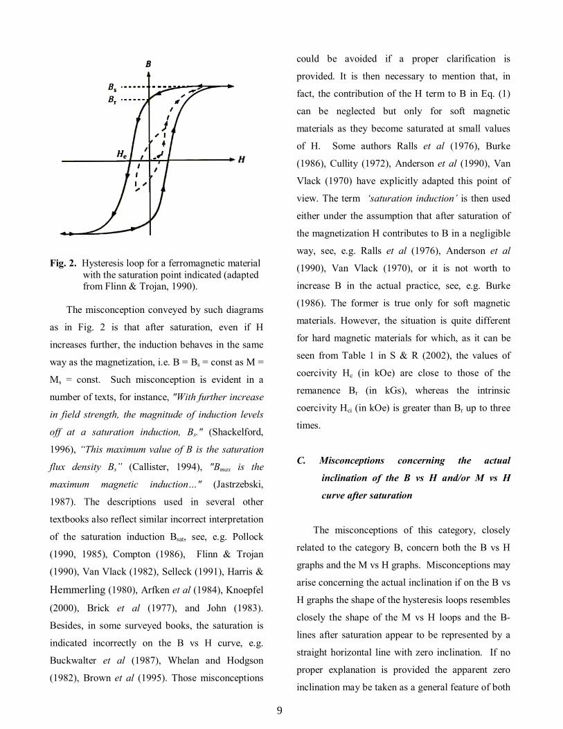
Fig. 2. Hysteresis loop for a ferromagnetic material with the saturation point indicated (adapted from Flinn & Trojan, 1990).

The misconception conveyed by such diagrams

as in Fig. 2 is that after saturation, even if H

increases further, the induction behaves in the same

way as the magnetization, i.e. B = Bs = const as M =

Ms = const. Such misconception is evident in a

number of texts, for instance, "With further increase

in field strength, the magnitude of induction levels

off at a saturation induction, Bs." (Shackelford,

1996), �This maximum value of B is the saturation

flux density Bs� (Callister, 1994), "Bmax is the

maximum magnetic induction�" (Jastrzebski,

1987). The descriptions used in several other

textbooks also reflect similar incorrect interpretation

of the saturation induction Bsat, see, e.g. Pollock

(1990, 1985), Compton (1986), Flinn & Trojan

(1990), Van Vlack (1982), Selleck (1991), Harris &

Hemmerling (1980), Arfken et al (1984), Knoepfel

(2000), Brick et al (1977), and John (1983).

Besides, in some surveyed books, the saturation is

indicated incorrectly on the B vs H curve, e.g.

Buckwalter et al (1987), Whelan and Hodgson

(1982), Brown et al (1995). Those misconceptions

could be avoided if a proper clarification is

provided. It is then necessary to mention that, in

fact, the contribution of the H term to B in Eq. (1)

can be neglected but only for soft magnetic

materials as they become saturated at small values

of H. Some authors Ralls et al (1976), Burke

(1986), Cullity (1972), Anderson et al (1990), Van

Vlack (1970) have explicitly adapted this point of

view. The term �saturation induction� is then used

either under the assumption that after saturation of

the magnetization H contributes to B in a negligible

way, see, e.g. Ralls et al (1976), Anderson et al

(1990), Van Vlack (1970), or it is not worth to

increase B in the actual practice, see, e.g. Burke

(1986). The former is true only for soft magnetic

materials. However, the situation is quite different

for hard magnetic materials for which, as it can be

seen from Table 1 in S & R (2002), the values of

coercivity Hc (in kOe) are close to those of the

remanence Br (in kGs), whereas the intrinsic

coercivity Hci (in kOe) is greater than Br up to three

times.

C. Misconceptions concerning the actual

inclination of the B vs H and/or M vs H

curve after saturation

The misconceptions of this category, closely

related to the category B, concern both the B vs H

graphs and the M vs H graphs. Misconceptions may

arise concerning the actual inclination if on the B vs

H graphs the shape of the hysteresis loops resembles

closely the shape of the M vs H loops and the B-

lines after saturation appear to be represented by a

straight horizontal line with zero inclination. If no

proper explanation is provided the apparent zero

inclination may be taken as a general feature of both

9

graphs applicable to all magnetic materials. The

opposite cases arise if on the M vs H graphs the

shape of the hysteresis loops resembles closely the

shape of the B vs H loops and the B-lines after

saturation appear to be represented by lines with a

noticeable inclination. Such cases amount to

mixing up the M vs H graphs with the B vs H

graphs and constitute misconceptions concerning

the features of the M vs H hysteresis loops. Several

cases of both versions of the misconceptions of this

category have been revealed by considering the

shape, inclination, and description of the B vs H and

M vs H graphs in the textbooks.

The misconceptions concerning the B vs H

graphs arise from the neglect of the difference

between the actual and apparent inclination of the

B-lines after saturation. After the magnetization

saturation is reached, M becomes constant: M = Ms.

Thus in the CGS units a further increase of H by 1

Oersted increases B by 1 Gauss, whereas in the SI

units, correspondingly, 1 A/m of H contributes 4π x

10-7 Tesla (i.e. the value of µo) to B. Hence, no

matter which units are used for the y- and x-axis, B

is exactly proportional to H and must be represented

by a straight line. However, the appearance of a

graph depends on the actual inclination of the B-line

after saturation, which is determined by the unit

elements chosen for the y-axis (yunit) and x-axis

(xunit), i.e. the scale used for the graph. To illustrate

how the extension line of the B vs H hysteresis loop

after saturation would look like for different scales,

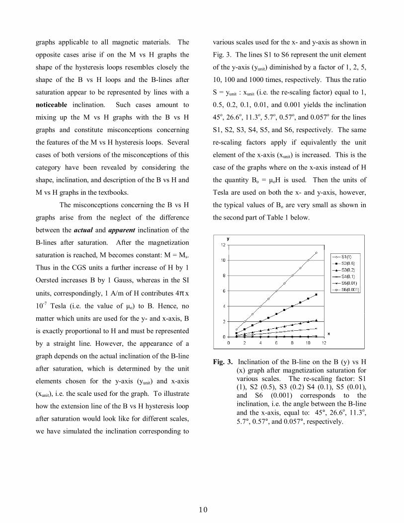
we have simulated the inclination corresponding to

various scales used for the x- and y-axis as shown in

Fig. 3. The lines S1 to S6 represent the unit element

of the y-axis (yunit) diminished by a factor of 1, 2, 5,

10, 100 and 1000 times, respectively. Thus the ratio

S = yunit : xunit (i.e. the re-scaling factor) equal to 1,

0.5, 0.2, 0.1, 0.01, and 0.001 yields the inclination

45o, 26.6o, 11.3o, 5.7o, 0.57o, and 0.057o for the lines

S1, S2, S3, S4, S5, and S6, respectively. The same

re-scaling factors apply if equivalently the unit

element of the x-axis (xunit) is increased. This is the

case of the graphs where on the x-axis instead of H

the quantity Bo = µoH is used. Then the units of

Tesla are used on both the x- and y-axis, however,

the typical values of Bo are very small as shown in

the second part of Table 1 below.

Fig. 3. Inclination of the B-line on the B (y) vs H

(x) graph after magnetization saturation for various scales. The re-scaling factor: S1 (1), S2 (0.5), S3 (0.2) S4 (0.1), S5 (0.01), and S6 (0.001) corresponds to the inclination, i.e. the angle between the B-line and the x-axis, equal to: 45°, 26.6o, 11.3o, 5.7°, 0.57°, and 0.057°, respectively.

10

11

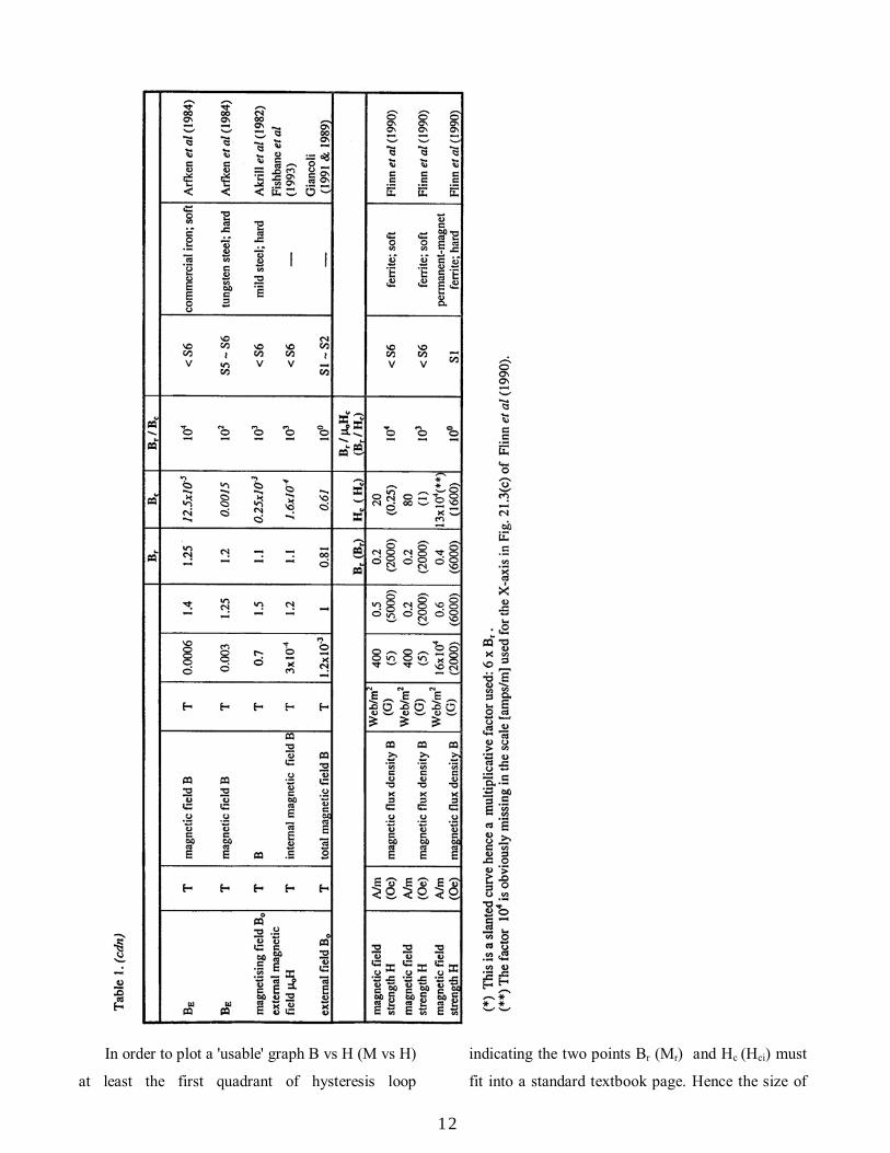
In order to plot a 'usable' graph B vs H (M vs H)

at least the first quadrant of hysteresis loop

indicating the two points Br (Mr) and Hc (Hci) must

fit into a standard textbook page. Hence the size of

12

the graph is approximately given by the values of Br

(Mr) and Hc (Hci) and thus different re-scaling

factors are required for different materials. An

approximate value of the suitable re-scaling factor

can be obtained by calculating the ratio Br / Hc

(CGS) or Br / µo Hc (SI) in the given standard units.

This method works well for the narrow and straight

hysteresis loops (soft materials) and the wide ones

(hard materials) for which the values of Br (Mr) are

not too different from their 'saturation' values. For a

slanted hysteresis loop, like in Fig. 4 - the B type,

with the values of Br (Mr) much smaller than their

'saturation' values a multiplicative factor of between

2 to 6 can be applied to Br (Mr), or alternatively the

values of Bs (Ms) may be used, if available. Let us

illustrate the effect of the re-scaling factors by

adopting the unit elements for the y-axis (yunit) and

x-axis (xunit) of equal length, say e.g. one centimeter.

Thus if the ratio Br / Hc (CGS) is, e.g. of the order

of (i) 103 or (ii) 104, the suitable re-scaling factor for

the graph would be (i) 0.001 or (ii) 0.0001. Such

graphs without re-scaling, i.e. using the 1 : 1 unit

labeling on the y- and x-axis, would require the

maximum on the y-axis, Ymax, of not less than (i) 10

m - the height of an average four-storey building or

(ii) 100 m - one-third of the height of Eiffel Tower

in Paris. On such graphs the actual inclination of

the B-lines after saturation would be exactly 45o.

The only drawback would be that they could not be

fitted into any textbook. By squeezing the graphs

along the y-axis (i) 1000 or (ii) 10000 times, a

'usable' size of the graph is obtained. BUT then the

corresponding apparent inclination almost vanishes

to (i) 0.057o - as for the S6 line in Fig. 3 or (ii)

0.0057o - which cannot be discernibly indicated in

Fig. 3. However, the apparent nearly zero

inclination of the B-lines after saturation, e.g. of the

type S5 and S6 in Fig. 3, should not be confused

with the exactly zero inclination of the M-lines after

saturation independent of the scale used.

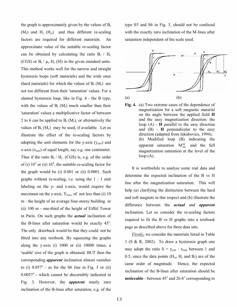
(a) (b)

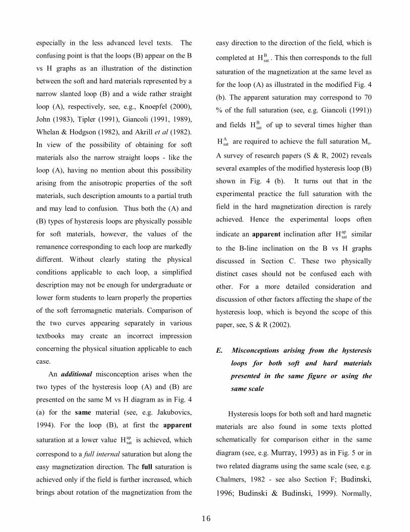
Fig. 4. (a) Two extreme cases of the dependence of magnetization for a soft magnetic material on the angle between the applied field H and the easy magnetization direction: the loop (A) - H parallel to the easy direction and (B) - H perpendicular to the easy direction (adapted from Jakubovics, 1994); (b) Modified loop (B) indicating the apparent saturation ap

satM and the full magnetization saturation at the level of the loop (A).

It is worthwhile to analyse some real data and

determine the expected inclination of the B vs H

line after the magnetization saturation. This will

help (a) clarifying the distinction between the hard

and soft magnets in this respect and (b) illustrate the

difference between the actual and apparent

inclination. Let us consider the re-scaling factors

required to fit the B vs H graphs into a textbook

page as described above for three data sets.

Firstly, we consider the materials listed in Table

1 (S & R, 2002). To draw a hysteresis graph one

may adopt the ratio S = yunit : xunit between 1 and

0.5, since the data points (Hci, Hc and Br) are of the

same order of magnitude. Hence, the expected

inclination of the B-lines after saturation should be

noticeable - between 45o and 26.6o corresponding to

13

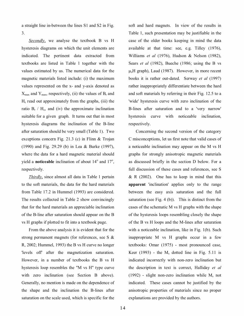
a straight line in-between the lines S1 and S2 in Fig.

3.

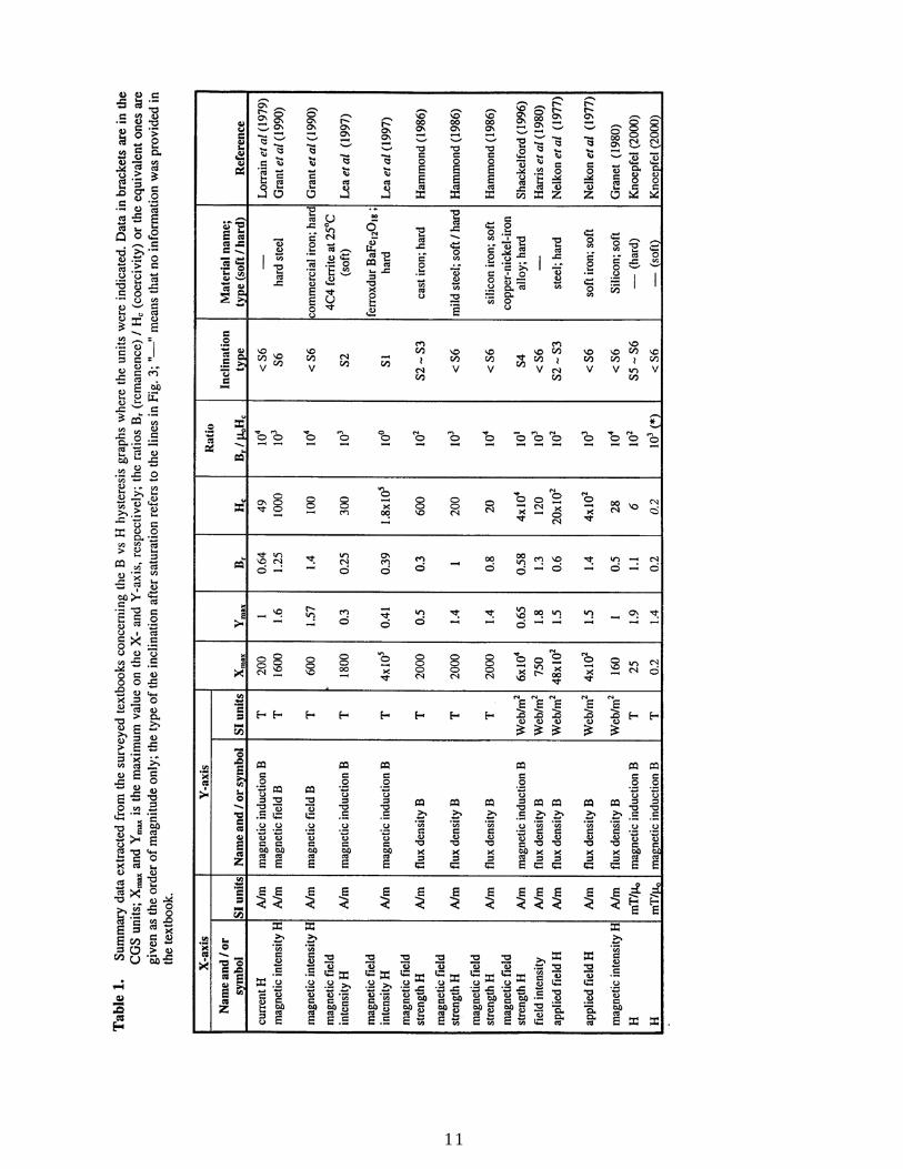
Secondly, we analyse the textbook B vs H

hysteresis diagrams on which the unit elements are

indicated. The pertinent data extracted from

textbooks are listed in Table 1 together with the

values estimated by us. The numerical data for the

magnetic materials listed include: (i) the maximum

values represented on the x- and y-axis denoted as

Xmax and Ymax, respectively, (ii) the values of Br and

Hc read out approximately from the graphs, (iii) the

ratio Br / Hc, and (iv) the approximate inclination

suitable for a given graph. It turns out that in most

hysteresis diagrams the inclination of the B-line

after saturation should be very small (Table 1). Two

exceptions concern Fig. 21.3 (c) in Flinn & Trojan

(1990) and Fig. 29.29 (b) in Lea & Burke (1997),

where the data for a hard magnetic material should

yield a noticeable inclination of about 14o and 17o,

respectively.

Thirdly, since almost all data in Table 1 pertain

to the soft materials, the data for the hard materials

from Table 17.2 in Hummel (1993) are considered.

The results collected in Table 2 show convincingly

that for the hard materials an appreciable inclination

of the B-line after saturation should appear on the B

vs H graphs if plotted to fit into a textbook page.

From the above analysis it is evident that for the

strong permanent magnets (for references, see S &

R, 2002; Hummel, 1993) the B vs H curve no longer

'levels off' after the magnetization saturation.

However, in a number of textbooks the B vs H

hysteresis loop resembles the "M vs H" type curve

with zero inclination (see Section B above).

Generally, no mention is made on the dependence of

the shape and the inclination the B-lines after

saturation on the scale used, which is specific for the

soft and hard magnets. In view of the results in

Table 1, such presentation may be justifiable in the

case of the older books keeping in mind the data

available at that time: see, e.g. Tilley (1976),

Williams et al (1976), Hudson & Nelson (1982),

Sears et al (1982), Bueche (1986; using the B vs

µoH graph), Laud (1987). However, in more recent

books it is rather out-dated. Serway et al (1997)

rather inappropriately differentiate between the hard

and soft materials by referring in their Fig. 12.5 to a

'wide' hysteresis curve with zero inclination of the

B-lines after saturation and to a 'very narrow'

hysteresis curve with noticeable inclination,

respectively.

Concerning the second version of the category

C misconceptions, let us first note that valid cases of

a noticeable inclination may appear on the M vs H

graphs for strongly anisotropic magnetic materials

as discussed briefly in the section D below. For a

full discussion of these cases and references, see S

& R (2002). One has to keep in mind that this

apparent 'inclination' applies only to the range

between the easy axis saturation and the full

saturation (see Fig. 4 (b)). This is distinct from the

cases of the schematic M vs H graphs with the shape

of the hysteresis loops resembling closely the shape

of the B vs H loops and the M-lines after saturation

with a noticeable inclination, like in Fig. 1(b). Such

inappropriate M vs H graphs occur in a few

textbooks: Omar (1975) - most pronounced case,

Keer (1993) - the Ms dotted line in Fig. 5.11 is

indicated incorrectly with non-zero inclination but

the description in text is correct, Halliday et al

(1992) - slight non-zero inclination while Ms not

indicated. These cases cannot be justified by the

anisotropic properties of materials since no proper

explanations are provided by the authors.

14

Table 2. Characteristics of the hysteresis loop for some permanent magnets; the ratios Br (remanence) / Hc (coercivity) or the equivalent ones are given as the order of magnitude only; Br and Hc values are taken from Table 17.2 of Hummel (1993); type of the inclination after saturation refers to the lines in Fig. 3.

Br [kG] Hc [Oe] Br / Hc Br [T] Hc [A/m] Br / µoHc Inclination type Material name 3.95 2400 1.6 0.4 1.9 x 105 1.7 S1 Ba-ferrite ( BaO.6Fe2O3 )

6.45 4300 1.5 0.6 3.4 x 105 1.4 S1 PtCo (77 Pt, 24 Co ) 13 14000 0.9 1.3 1.1 x 106 0.9 S1 Iron-Neodymium-Boron

( Fe14Nd2B1 )

9 51 176 0.9 4 x 103 179 S5 Steel ( Fe-1%C ) 13.1 700 19 1.3 5.6 x 104 18 S4 ~ S5 Alnico 5 DG

( 8 Al, 15 Ni, 24 Co, 3 Cu, 50 Fe )

10 450 22 1 3.6 x 104 22 S4 ~ S5 Vically 2 ( 13V, 52 Co, 35 Fe)

D. Misconceptions concerning the dependence of

the shape of the hysteresis loops on the

direction of the applied field

Another source of confusion may arise due to

the fact that the values of Br and Hc for the same

material may be noticeably different for different

physical conditions to which a given material may

be subjected. Even the same chemically material

may be behave either as a magnetically soft or hard

material, depending on the physical conditions

applied. These aspects will be discussed in detail in

S & R (2002). Here let us consider the possible

different shapes of the hysteresis loop as illustrated

in Fig. 4 for soft materials. According to Jakubovics

(1994) the M vs H loops (A) and (B) in Fig. 4 (a)

are for the same material, but the loop (A)

corresponds to a greater permeability and saturation

value Ms than the loop (B). A curious student

encountering in various books one of the two

distinct types of the hysteresis loop, i.e. in one book

the A-type graph and in another book the B-type

graph - each supposedly for the soft materials,

would certainly be puzzled if no proper explanation

on the physical reasons of such difference is

provided. This unfortunately is the case in some

textbooks (see below). In fact, on either graph: B vs

H or M vs H, the loop (A) is obtained if the field H

is applied parallel to the easy direction (ED) of

magnetization in the material, whereas the loop (B)

is obtained if the field H is applied either parallel to

the hard direction (HD) of magnetization or

perpendicular to the easy direction (see, e.g.,

Cullity, 1972; Jakubovics, 1994; den Broeder &

Draaisma, 1987; Babkair & Grundy, 1987). One

must be careful not to confuse the meaning of

'parallel' and ' perpendicular' directions, since in

some materials the easy direction is perpendicular

to the film surface, and thus the notation used on the

graphs: ⊥ and - referred to the film surface, may

be easily confused with the case: H ED (S & R,

2002).

It appears from our text survey that the

hysteresis loops, both the type: B vs H and M vs H,

for magnetically soft materials are usually presented

in a simplified way as either the loop (A) or (B) in

Fig. 4 (a), with the loop (A) being used more often,

15

especially in the less advanced level texts. The

confusing point is that the loops (B) appear on the B

vs H graphs as an illustration of the distinction

between the soft and hard materials represented by a

narrow slanted loop (B) and a wide rather straight

loop (A), respectively, see, e.g., Knoepfel (2000),

John (1983), Tipler (1991), Giancoli (1991, 1989),

Whelan & Hodgson (1982), and Akrill et al (1982).

In view of the possibility of obtaining for soft

materials also the narrow straight loops - like the

loop (A), having no mention about this possibility

arising from the anisotropic properties of the soft

materials, such description amounts to a partial truth

and may lead to confusion. Thus both the (A) and

(B) types of hysteresis loops are physically possible

for soft materials, however, the values of the

remanence corresponding to each loop are markedly

different. Without clearly stating the physical

conditions applicable to each loop, a simplified

description may not be enough for undergraduate or

lower form students to learn properly the properties

of the soft ferromagnetic materials. Comparison of

the two curves appearing separately in various

textbooks may create an incorrect impression

concerning the physical situation applicable to each

case.

An additional misconception arises when the

two types of the hysteresis loop (A) and (B) are

presented on the same M vs H diagram as in Fig. 4

(a) for the same material (see, e.g. Jakubovics,

1994). For the loop (B), at first the apparent

saturation at a lower value apsatH is achieved, which

correspond to a full internal saturation but along the

easy magnetization direction. The full saturation is

achieved only if the field is further increased, which

brings about rotation of the magnetization from the

easy direction to the direction of the field, which is

completed at BsatH . This then corresponds to the full

saturation of the magnetization at the same level as

for the loop (A) as illustrated in the modified Fig. 4

(b). The apparent saturation may correspond to 70

% of the full saturation (see, e.g. Giancoli (1991))

and fields BsatH of up to several times higher than

AsatH are required to achieve the full saturation Ms.

A survey of research papers (S & R, 2002) reveals

several examples of the modified hysteresis loop (B)

shown in Fig. 4 (b). It turns out that in the

experimental practice the full saturation with the

field in the hard magnetization direction is rarely

achieved. Hence the experimental loops often

indicate an apparent inclination after apsatH similar

to the B-line inclination on the B vs H graphs

discussed in Section C. These two physically

distinct cases should not be confused each with

other. For a more detailed consideration and

discussion of other factors affecting the shape of the

hysteresis loop, which is beyond the scope of this

paper, see, S & R (2002).

E. Misconceptions arising from the hysteresis

loops for both soft and hard materials

presented in the same figure or using the

same scale

Hysteresis loops for both soft and hard magnetic

materials are also found in some texts plotted

schematically for comparison either in the same

diagram (see, e.g. Murray, 1993) as in Fig. 5 or in

two related diagrams using the same scale (see, e.g.

Chalmers, 1982 - see also Section F; Budinski,

1996; Budinski & Budinski, 1999). Normally,

16

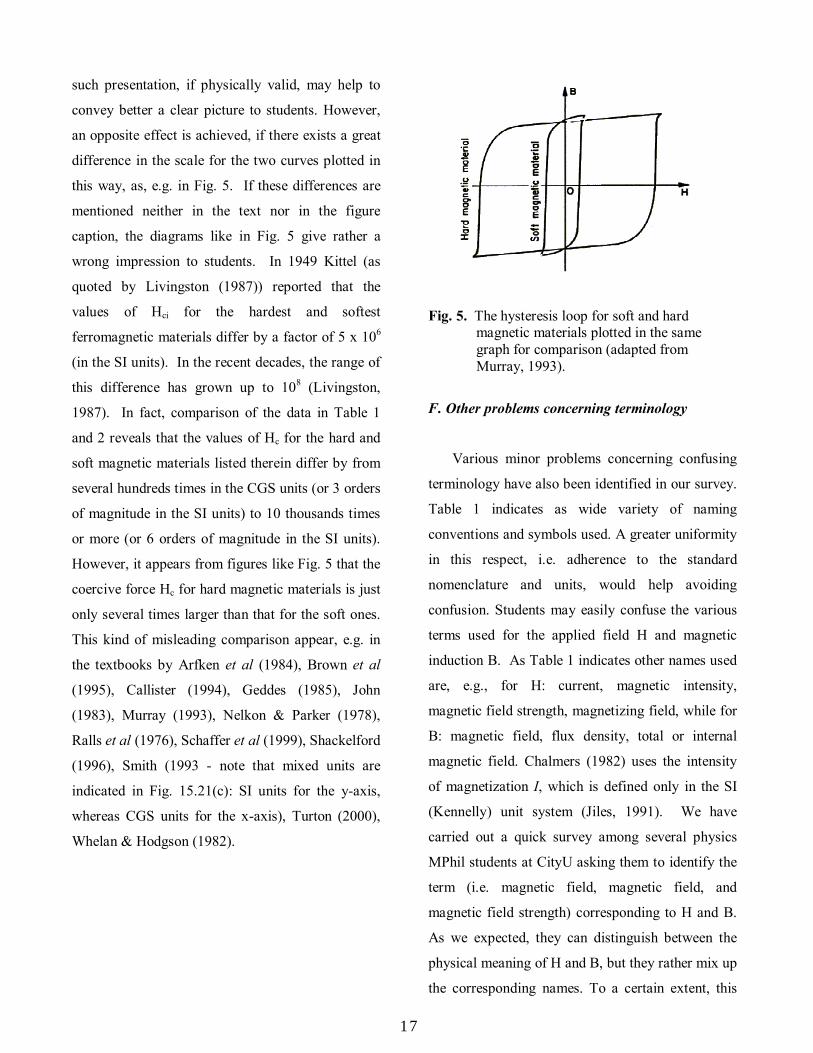
such presentation, if physically valid, may help to

convey better a clear picture to students. However,

an opposite effect is achieved, if there exists a great

difference in the scale for the two curves plotted in

this way, as, e.g. in Fig. 5. If these differences are

mentioned neither in the text nor in the figure

caption, the diagrams like in Fig. 5 give rather a

wrong impression to students. In 1949 Kittel (as

quoted by Livingston (1987)) reported that the

values of Hci for the hardest and softest

ferromagnetic materials differ by a factor of 5 x 106

(in the SI units). In the recent decades, the range of

this difference has grown up to 108 (Livingston,

1987). In fact, comparison of the data in Table 1

and 2 reveals that the values of Hc for the hard and

soft magnetic materials listed therein differ by from

several hundreds times in the CGS units (or 3 orders

of magnitude in the SI units) to 10 thousands times

or more (or 6 orders of magnitude in the SI units).

However, it appears from figures like Fig. 5 that the

coercive force Hc for hard magnetic materials is just

only several times larger than that for the soft ones.

This kind of misleading comparison appear, e.g. in

the textbooks by Arfken et al (1984), Brown et al

(1995), Callister (1994), Geddes (1985), John

(1983), Murray (1993), Nelkon & Parker (1978),

Ralls et al (1976), Schaffer et al (1999), Shackelford

(1996), Smith (1993 - note that mixed units are

indicated in Fig. 15.21(c): SI units for the y-axis,

whereas CGS units for the x-axis), Turton (2000),

Whelan & Hodgson (1982).

Fig. 5. The hysteresis loop for soft and hard magnetic materials plotted in the same graph for comparison (adapted from Murray, 1993).

F. Other problems concerning terminology

Various minor problems concerning confusing

terminology have also been identified in our survey.

Table 1 indicates as wide variety of naming

conventions and symbols used. A greater uniformity

in this respect, i.e. adherence to the standard

nomenclature and units, would help avoiding

confusion. Students may easily confuse the various

terms used for the applied field H and magnetic

induction B. As Table 1 indicates other names used

are, e.g., for H: current, magnetic intensity,

magnetic field strength, magnetizing field, while for

B: magnetic field, flux density, total or internal

magnetic field. Chalmers (1982) uses the intensity

of magnetization I, which is defined only in the SI

(Kennelly) unit system (Jiles, 1991). We have

carried out a quick survey among several physics

MPhil students at CityU asking them to identify the

term (i.e. magnetic field, magnetic field, and

magnetic field strength) corresponding to H and B.

As we expected, they can distinguish between the

physical meaning of H and B, but they rather mix up

the corresponding names. To a certain extent, this

17

finding is a reflection of the unhealthy situation

prevailing in the textbooks (see Table 1). The

existing variety of conventions used for the

quantities H, B and M hampers the understanding of

physics, especially even more seriously for the

lower form students.

The improper use of the term 'polarization' to

interpret the B vs H curve occurs in Abele (1993).

Normally, �polarization� is used to describe the

electric quantities rather than the magnetic ones.

�Polarization� of dielectric materials is an analogue

quantity to �magnetization� in magnetism, however,

the two terms are not equivalent. Besides, John

(1983) denotes on the y-axis the magnetization

confusingly as B, �magnetization induced B�, and

describes the x-axis as: �magnetizing force H�.

Improper use of symbols leads to confusion like,

e.g., "saturation magnetization� denoted as �Bs" by

Murray (1993). Another confusing notion is used by

Granet (1980): "magnetization current", which

means the electric current, which induces H, which,

in turn, magnetizes the sample. Such terminology

mixing up the magnetic and electrical notions and/or

quantities may be confusing for students and should

be avoided for pedagogical reasons. Another

example of confusion is: "If the field intensity is

increased to its maximum in this direction, then

reversed again �� (Thornton & Colangelo, 1985).

In fact, there is no �maximum limit� for the applied

field, apart from the limits imposed by the

experimental equipment.

4. A survey of students� understanding of the

hysteresis loop

The effect of the confusion and misconceptions

existing in textbooks on the students� understanding

of the hysteresis loop can be assessed by analysing

the results of examinations or tests. In our lecture

notes for the condensed matter physics course

(Rudowicz, 2000; available from CZR upon

request) we have presented clearly, so briefly, the

distinction between the pertinent notions as well as

warned students about the misinterpretations

discussed in Section A above. However, the analysis

of the results of the CMP examination carried out in

May 2001 indicates that the message has not

reached some students. Eleven students out of total

15 attempted the two questions concerning the

hysteresis loop, stated as follows:

a) Draw a schematic diagram of the magnetic

field intensity inside a material B versus the

(external) applied magnetic field strength H

for an initially unmagnetized ferromagnetic

material.

b) Define the following quantities: (1) the

saturation magnetic field, (2) the remanence,

and (3) the coercive force. Indicate these

quantities on the diagram B versus H (the

hysteresis loop).

Most of them performed not too well since they

often misinterpreted the characteristics of the

hysteresis loop. Common mistakes include, e.g., (a)

mixing up the coercivity with the remanence, (b)

indicating a 'maximum' value of the applied field H

and the magnetic induction B, (c) stating that both B

and M are equal to zero at Hc. Obviously, some of

these misconceptions concerning the hysteresis loop

are quite close to the ones existing in the surveyed

textbooks as discussed above. However, such

misconceptions by our students may not originate

from any insufficient clarifications of the major

18

terms in the books they might have used, but rather

are due to the students� attitudes to learning. In

general, a good interpretation of a particular topic in

textbooks may help teachers to increase the

efficiency of teaching (and save their time which

would have been used for clarifications), whereas

students to improve their understanding of the

physical concepts beyond the level presented at the

lectures. On the contrary, the improper definitions

of the crucial terms and/or outright misconceptions

will most certainly hamper the students�

understanding and may contribute to a reduced

interest in further physics studies, especially at a

lower level of students' education (Hubisz, 2000).

5. Conclusions and suggestions

It appears that the two possible ways of

presenting the hysteresis loop for ferromagnetic

materials, B vs H and M vs H, are, to a certain

extent, confused each with other in several

textbooks. This leads to various misconceptions

concerning the meaning of the physical quantities as

well as the characteristic features of the hysteresis

loop for the soft and hard magnetic materials. We

suggest that the name �coercive force� (or

�coercivity�) and the symbol Hc , correctly defined

for the B vs H curve, should not be used if referred

to the M vs H curve. Using in the latter case the

adjective 'intrinsic' and the symbol Hci is strongly

recommended. It may help avoiding the

misconceptions discussed above and reduce the

present confusion widely spread in the textbooks.

Hence the authors and editors should pay more

attention to proper definitions of the terms involved.

Interestingly, among the books by Beiser (1986,

1991, 1992), the book (1986) belongs to the

�misinterpretation sample�, while the two later

books (1991, 1992) are correct in this aspect. It is

hoped that by bringing the problems in questions to

the attention of physics teachers and students, the

correct interpretation of the hysteresis loop will

prevail in future.

Our survey of textbooks reveal several deeper

pedagogical issues related to the presentation of the

hysteresis loop, which may apply to various other

topics as well. One is the distinction between the

�exact� and �approximate� quantities and the related

description of a physical situation. In the present

case we have considered the approximation �H

small as compared with M�, leading to B ≈ µoM and

Hc ≈ Hci for soft magnetic materials. If the

conditions for which a given approximation is valid

are not clearly stated, the approximate picture may

be implicitly taken as a representation of the exact

situation. The consequences of such misleading

approach may be wide-ranging - from imprinting

misconceptions, i.e. false images, in the students�

minds to misinterpretation of the properties of one

class of materials (here, soft magnets) as being

equivalent to those of another class (here, hard

magnets).

The inherent danger in using �schematic�

diagrams for presentation of the dependencies

between various physical quantities is another

important issue. Having no units and values

provided for the y- and x-axis constitutes a

detachment from a real physical situation. It may

not only hamper students� understanding of the

underlying physics, but also lead to false

impressions about the relationships between the

quantities involved and, in consequence, create

misconceptions. This is best exemplified for the

present topic by Fig. 4 and Fig. 5. The drawbacks of

19

�schematic� representation of each hysteresis loops

are compounded by the �space saving� and using a

combined diagram like in Fig. 5, which implies the

same limits and values are applicable for both types

of magnetic materials. As we amply illustrated

above this is far from the true situation. Schematic

diagrams which do not reflect correctly the

underlying physical situation become a piece of

graphic art only. Providing neither symbols nor

description of the quantities on the x- and y-axis of a

graph (see, e.g. Fig. 15.9 in Machlup, 1988) should

also be avoided in physics text as an inappropriate

from both scientific and pedagogical point of view.

Finally, let us mention the idea of creating a

website listing errors and misconceptions in

textbooks. The individual lecturers could add up

their knowledge in this respect to a well organized

structure listing various topics. We have had

preliminary talks within CityU about the idea of

having such a website residing on the CityU

computer network but the response was rather

muted. Our initial Internet search for the keywords:

'errors', 'misprints', 'corrigenda', 'errata', has,

however, revealed, no relevant sites. A similar idea

was proposed by Hubisz (2000) concerning science

textbooks. Interestingly we have located this

website due to letter in American Physical Society

Newsletter (April, 2001, p.4). Since the URL

address was misprinted, we have tracked this site

down via the university name (North Carolina State

University). Only recently by chance we have learnt

of the existing website listing errors in physics

textbooks:

(http://www.escape.ca/~dcc/phys/errors.html). It

appears that the benefits of such website for teachers

and students in improving general understanding of

physics may be substantial.

Acknowledgements This work was supported by the City University

of Hong Kong through the research grant: QEF #

8710126.

References Abele M G 1993 Structures of Permanent Magnets Generation of Uniform Fields (New York: John Wiley &

Sons) p 33-35 Aharoni A 1996 Introduction to the Theory of Ferromagnetism (Oxford: Clarendon Press) p 1-3 Akrill T B, Bennet G A G and Millar C J 1982 Physics (London: Edward Arnold) p 234 Anderson H L 1989 A Physicist�s Desk Reference Physics Vade Mecum (New York: American Institute of

Physics) Anderson J C, Leaver K D, Rawlings R D and Alexander J M 1990 Materials Science (London: Chapman and

Hall) p 501-502 Anderson J P and Blotzer R J 1999 Permeability and hysteresis measurement The Measurement,

Instrumentation, and Sensors Handbook ed J G Webster (Florida: CRC Press) p 49-6-7 Arfken G B, Griffing D F, Kelly D C and Priest J 1984 University Physics (Orlando: Academic Press) p 694-

697 Arrott A S 1983 Ferromagnetism in Concise Encyclopedia of Solid State Physics ed R G Lerner & G L Trigg

(London: Addison-Wesley Publishing) p 97-101 Babkair S S and Grundy P J 1987 Multilayer ferromagnetic thin film supersturctures -Co/Cr in Proceedings of

the International Symposium on Physics of Magnetic Materials ed M Takahashi et al (Singapore: World Scientific) p 267-270

Barger V D and Olsson M G 1987 Classical Electricity and Magnetism (Boston: Allyn and Bacon) p 318-319

20

Beiser A 1986 Schaum's outline of Theory and Problems of Applied Physics (Singapore: McGraw-Hill ) p 195-197

Beiser A 1991 Physics (Massachusetts: Addison-Wesley) p 546-548 Beiser A 1992 Modern Technical Physics (Massachusetts: Addison-Wesley) p 576-578 Besancon R M 1985 The Encyclopedia of Physics (New York: Van Nostrand Reinhold) p 440 Brick R M, Pense A W and Gordon R B 1977 Structure and Properties of Engineering Materials (New York:

McGraw-Hill) p 33-34 Brown W, Emery T, Gregory M, Hackett R and Yates C 1995 Advanced Physics (Singapore: Longman) p 226-

227 Buckwalter G L and Riban D M 1987 College Physics (New York: McGraw-Hill Book Company) p 511-512 Budinski K G 1996 Engineering Materials Properties and Selection (New Jersey: Prentice Hall) p 28 Budinski K G and Budinski M K 1999 Engineering Materials Properties and Selection (New Jersey: Prentice

Hall) p 29-30 Bueche F J 1986 Introduction to Physics for Scientists and Engineers (New York: Glencoe/McGraw- Hill) p

522 Burke H E 1986 Handbook of Magnetic Phenomena (New York: Van Nostrand Reinhold) p 63-64 Callister, Jr W D 1994 Material Science and Engineering An Introduction (New York: John Wiley & Sons) p

673-675 Chalmers B 1982 The Structure and Properties of Solids (London: Heyden) p 46-49 Compton A J 1986 Basic Electromagnetism and its Applications (Berkshire: Van Nostrand Reinhold) p 97-98 Cullity B D 1972 Introducton to Magnetic Materials (Massachusetts: Addison-Wesley) p 18-19 Daintith J 1981 Dictionary of Physics (New York: Facts On File) p. 88 Dalven R 1990 Introduction to Applied Solid State Physics (New York: Plenum Press) p 367-376 den Broeder F J A and Draaisma H J G 1987 Structure and magnetism of polycrystalline multilayers

containing ultrathin Co or Fe in Proceedings of the International Symposium on Physics of Magnetic Materials ed M Takahashi et al (Singapore: World Scientific) p 234-239

Donoho P L 1983 Hysteresis in Concise Encyclopedia of Solid State Physics ed R G Lerner & G L Trigg (London: Addison-Wesley Publishing) p 122-123

Dugdale D 1993 Essential of electromagnetism (New York: American Institute of Physics) p 198-199 Elliott R J and Gibson A F 1978 An Introduction to Solid State Physics and its Applications (London: English

Language Book Society) p 464-466 Elliott S R 1998 The Physics and Chemistry of Solids (Chichester: John Wiley & Sons) p 630 Elwell D and Pointon A J 1979 Physics for Engineers and Scientists (Chichester: Ellis Horwood) p 307-308 Fishbane P M, Gasiorowicz S and Thornton S T 1993 Physics for Scientists and Engineers (New Jersey:

Prentice Hall) p 947-948. Flinn R A and Trojan P K 1990 Engineering Materials and Their applications (Dallas: Houghton Mifflin) p

S178-S182 Geddes S M 1985 Advanced Physics (Houndmills: Macmillan Education) p 57-59 Giancoli D C 1989 Physics for Scientists and Engineers with Modern Physics (New Jersey: Prentice Hall) p

662-663 Giancoli D C 1991 Physics Principles with Applications (New Jersey: Prentice Hall) p 529-531

Granet I 1980 Modern Materials Science (Virginia: Prentice-Hall) p 422-427 Grant I S and Phillips W R 1990 Electromagnetism (Chichester: John Wiley & Sons) p 201-242 Gray H J and Isaacs A 1975 A New Dictionary of Physics (London: Longman) p 268 Halliday D, Resnick R and Krane K S 1992 Physics Vol.2 (New York: John Wiley & Sons) p 814 Hammond P 1986 Electromagnetism for Engineers An Introductory Course (Oxford: Pergamon press) p 134-

137 Harris N C and Hemmerling E M 1980 Introductory Applied Physics (New York: McGraw-Hill) p 570-571 Hickey & Schibeci 1999 Phys. Educ. 34 383-388 Hoon S R and Tanner B K 1985 Phys. Educ. 20 61-65 Hubisz J L 2000 Review of Middle School Physical Science Texts (http://www.psrc-

online.org/curriculum/book.html) - accessed June 2001 p 1-98 Hudson A and Nelson R 1982 University Physics (San Diego: Harcourt Brace Jovanovich) p 669

21

Hummel R E 1993 Electronic Properties of Materials (Berlin: Springer-Verlag) p 314, 319 Jakubovics J P 1994 Magnetism and Magnetic Materials (Cambridge: The Institute of Materials) Jastrzebski Z D 1987 The Nature and Properties of Engineering materials (New York: John Wiley & Sons) p

482-485 Jiles D 1991 Introduction to Magnetism and Magnetic Materials (London: Chapman & Hall) p 70-73 John V B 1983 Introduction to Engineering Materials (London: Macmillan) p 130-131 Keer H V 1993 Principles of the Solid State (New York: John Wiley and Sons) p 235-236 Kittel C 1996 Introduction to Solid State Physics (New York: John Wiley & Sons) p 468-470 Knoepfel H E 2000 Magnetic fields A Comprehensive Theoretical Treatise for Practical Use (New York: John

Wiley & Sons) p 486-491 Lapedes D N 1978 Dictionary of Physics and Mathematics (New York: McGraw-Hill) p 469 Laud B B 1987 Electromagnetics (New York: John Wiley & Sons) p 162-163 Lea S M and Burke J R 1997 Physics The Nature of Things (New York: West Publishing) p 941-942 Lerner R G and Trigg G L 1991 Encyclopedia of Physics (New York: VCH Publishers) p 692-693 Levy R A 1968 Principles of Solid State Physics (New York: Academic Press) p 258-260 Livingston 1987 Upper and lower limits of hard and soft magnetic properties in Proceedings of the

International Symposium on Physics of Magnetic Materials ed M Takahashi et al (Singapore: World Scientific) p 3-16

Lord M P 1986 Dictionary of Physics (London: Macmillan) p 140 Lorrain P and Corson D R 1979 Electromagnetism (San Francisco: W.H. Freeman and Company) p 342-345 Lovell M C, Avery A J and Vernon M W 1981 Physical Properties of Materials (New York: Van Nostrand

Reinhold) p 189 Machlup S 1988 Physics (New York: John Wiley & Sons) p 459 Meyers R A 1990 Encyclopedia of Modern Physics (San Diego: Harcourt Brace Jovanovich) p 254-255 Murray G T 1993 Introduction to Engineering Materials Behavior, Properties, and Selection (New York:

Marel Dekker) p 529-531 Nelkon M and Parker P 1978 Advanced Level Physics (London: Heinemann Educational Books) p 843 Omar M A 1975 Elementary Solid State Physics: Principles and Applications (Massachusetts: Addison-

Wesley) p 461 Ouseph P J 1986 Technical Physics (New York: Delmar) p 537-538 Parker S P 1993 Encyclopedia of Physics (New York: McGraw-Hill) p 733 Pitt V H 1986 The Penguin Dictionary of Physics (Middlesex: Penguin books) p 186-187 Pollock D D 1985 Physical of Materials for Engineers Vol. II (Boca Raton: CRC Press) p 138-139 Pollock D D 1990 Physics of Engineering Materials (New Jersey: Prentice Hall) p 587-589 Ralls K M, Courtney T H and Wulff 1976 Introduction to Materials Science and Engineering (New York: John

Wiley & Sons) p 575-577 Rhyne J J 1983 Magnetic Materials in Concise Encyclopedia of Solid State Physics ed R G Lerner & G L

Trigg (London: Addison-Wesley Publishing) p 160-162 Rogalski M S and Palmer S B 2000 Solid-State Physics (Australia: Gordon and Breach Science Publishers) p

379 Rudowicz C, 2001, Lecture Notes: Condensed Matter Physics, City University of Hong Kong, unpublished. Schaffer J P, Saxena a, Antolovich S D, Sanders Jr. T H and Warner S B 1999 The Science and Design of

Engineering Materials (Boston: McGraw-Hill) p 527-530 Sears F W, Zemansky M W and Young H D 1982 University Physics (California: Addison-Wesley) p 673-674 Selleck E 1991 Technical Physics (New York: Delmar) p 879-880 Serway R A 1990 Physics for Scientists & Engineers with Modern Physics (Philadelphia: Saunders College) p

857-859 Serway R A, Moses C J and Moyer C A 1997 Modern Physics (Fort: Saunders College) p 481-483 Shackelford J F 1996 Introduction to Materials Science for Engineers (New Jersey: Prentice Hall) p 507-512 Skomski R and Coey J M D 1999 Studies in Condensed Matter Physics Permanent Magnetism (Bristol:

Institute of Physics) p 169-174 Smith W F 1993 Foundations of Materials Science and Engineering (New York: McGraw-Hill) p 827-828 Sung H W F and Rudowicz C 2002 J. Mag. Magn. Mat. - submitted Feb 2002

22

Thornton P A and Colangelo V J 1985 Fundamentals of Engineering Materials (New Jersey: Prentice-Hall) p 372-373

Tilley D E 1976 University Physics for Science and Engineering (California: Cummings Publishing) p 532-534Tipler P A 1991 Physics for Scientists and Engineers (New York: Worth) p 886-888 Turton R 2000 The Physics of Solids (Oxford: Oxford University Press) p 237 Van Vlack L H 1970 Materials Science for Engineers (Menlo Park: Addison-Wesley) p 327-328 Van Vlack L H 1982 Materials for Engineering: Concepts and Applications (Menlo Park: Addison-Wesley) p

544 Vermariën H, McConnell E and Li Y F 1999 Reading / recording devices The Measurement, Instrumentation,

and Sensors Handbook ed J G Webster (Florida: CRC Press) p 96-24-25 Wert C A and Thomson R M 1970 Physics of Solids (New York: McGraw-Hill) p 455-456 Whelan P M and Hodgson M J 1982 Essential Principles of Physics (London: John Murray) p 429 Williams J E Trinklein F E and Metcalfe H C 1976 Modern Physics (New York: Holt, Rinehart and Winston) p

468 Wilson I 1979 Engineering Solids (London: McGraw Hill) p 119-123

23

Appendix I. List of other surveyed textbooks not included in the references The list of textbooks surveyed, in which no relevant misconceptions and/or confusions were identified and

which are not quoted in text, is given below.

Benson H 1991 University Physics (New York: John Wiley & Sons) p 653 Blakemore J S 1985 Solid State Physics (Cambridge: Cambridge University Press) p 450 Bube R H 1992 Electrons in Solids An Introductory Survey (Boston: Academic Press) p 261-262 Burns G 1985 Solid State Physics (Orlando: Academic Press) p 614 Christman J R 1988 Fundamentals of Solid State Physics (New York: John Wiley & Sons) p 369 Coren R L 1989 Basic Engineering Electromagnetics An Applied Approach (New Jersey: Prentice Hall) p 76-

77 Craik D 1995 Magnetism Principles and Applications p 105 Crangle J 1991 Solid State Magnetism (London: Edward Arnold) p 168-171 Dekker A J 1960 Solid State Physics (London: Macmillan & Co) p 476 Enz C P 1992 Lecture Notes in Physics vol. 11 A Course on Many-Body Theory Applied to Solid-State Physics

(Singopore: World Scientific) p 267 Feynman Leighton and Sands 1989 Commemorative Issue The Feynman Lectures on Physics Vol. II (Addison-

Wesley: California) p 36-5-36-9 Gershenfeld N 2000 The Physics of Information Technology (Cambridge: Cambridge University Press) p 193 Guinier A and Jullien R 1989 The Solid State From Superconductors to Superalloys (Oxford: Oxford

University Press) p 163-166 Halliday D, and Resnick R 1978 Physics Part I and II (New York: John Wiley & Sons) p 827 Hammond P and Sykulski J K 1994 Engineering Electromagnetism Physical Processes and Computation

(Oxford: Oxford University Press) p 223-225 Hook J R and Hall H E 1991 Solid State Physics (Chichester: John Wiley & Sons) p 251 Joseph A, Pomeranz K, Prince J and Sacher D 1978 Physics for Engineering Technology (New York: John

Wiley & Sons) p 442 Kahn O 1999 Magnetic anisotropy in molecule-based magnets in Metal-Organic and Organic Molecular

Magnets ed P Day and A E Underhill (Cambridge: Royal Society of Chemistry) p 150-168 Kinoshita M 1999 Molecular-based magnets: setting the scene in Metal-Organic and Organic Molecular

Magnets ed P Day and A E Underhill (Cambridge: Royal Society of Chemistry) p 4-21 Lorrain P and Corson D R 1979 Electromagnetism (San Francisco: W.H. Freeman and Company) p 342-345 Marion J B and Hornyak W F 1984 Principles of Physics (Philadelphia: Saunders College Publishing) p 750 Myers H P 1991 Introductory Solid State Physics (London: Taylor & Francis) p 377 Narang B S 1983 Material Science and Processes (Delhi: CBS) p 66-67 Ohanian H C 1989 Physics Vol.2 (New York: W.W. Norton) p 818 Parker S P 1988 Solid-State Physics Source Book (New York: Mcgraw-Hill) p 223-230 Radin S H and Folk R T 1982 Physics for Scientists and Engineers (New Jersey: Prentice-Hall) p 657 Rosenberg H M 1983 The Sold State (Oxford: Clarendon) p 202 Rudden M N and Wilson J 1993 Elements of Solid State Physics (Chichester: John Wiley & Sons) p 103, 109 Schneider, Jr S J, Davis J R, Davidson G M, Lampman S R, Woods M S and Zorc T B 1991 Engineered

Materials Handbook Vol. 4 (USA: ASM International) p 1162 Swartz C E 1981 Phenomenal Physics (New York: John Wiley & Sons) p 609 Tanner B K 1995 Introduction to the Physics Electrons in Solids (Cambridge: Cambridge University Press) p

181-182 Tippens P E 1991 Physics (New York: Glencoe/McGraw-Hill) p 671-672 Van Vlack L H 1989 Elements of Materials Science and Engineering (Menlo park: Addison-Wesley) p 450-453Vonsovskii S V 1974 Magnetism Vol. One (New York: John Wiley & Sons) p 42-43 Young H D and Freeman R A 1996 Extended Version with Modern Physics: University Physics

(Massachusetts: Addison-wesley) p 926 Zafiratos C D 1985 Physics (New York: John Wiley & Sons) p 673-674

24