A CFD Simulation Analysis of the Water Volumetric Fraction

A CFD SIMULATION ANALYSIS OF THE WATER VOLUMETRIC FRACTIONDISTRIBUTION IN THE RUNNER OF A TURGO TYPE TURBINE DESIGNED WITH

AN INTEGRATED DIMENSIONAL METHODOLOGY

Jorge Luis Clarembaux CorreaMechanical Engineering Conversion Laboratory

Simon Bolivar UniversityValle de Sartenejas, VenezuelaEmail: [email protected]

Jesus de AndradeMechanical Engineering Conversion Laboratory

Simon Bolivar UniversityValle de Sartenejas, VenezuelaEmail: [email protected]

Sergio CroquerMechanical Engineering Conversion Laboratory

Simon Bolivar UniversityValle de Sartenejas, Venezuela

Email: [email protected]

Miguel AsuajeMechanical Engineering Conversion Laboratory

Simon Bolivar UniversityValle de Sartenejas, Venezuela

Email: [email protected]

ABSTRACTOur previous work, on development of a design

methodology inspired in the analysis of One-Dimensionaland Three-dimensional Theories [1], allowed to obtain a TurgoType Turbine (TTT) bucket using 8 geometric parameters asa function of the jet diameter, and Rankine Ovoids potentialflow. CFD models under steady state regime [2] made possibleto verify deduced expressions for torque, output power andhydraulic efficiency. In this paper, the effects of the watervolumetric fraction distribution in the runner have beenincluded, which are significantly conclusive to understandthe runner hydrodynamic behavior and highlighted severaloptimizations to the performance equations that could beconsidered as a potential novelty for these turbines. In the sameway, an influence study of nozzle parameters determined that themost profitable performance is achieved for an absolute velocityangle coming from the jet of 19.8o. Finally, several differencesin the flow distribution in the runner were evaluated through anon-steady state regime CFD simulation, when comparing withthe steady state.

Keywords: hydraulic turbine, Turgo Type Turbine, Rankine

oval bodies, performance analysis.

NOMENCLATURESymbolsc absolute velocity; [m/s]d jet diameter; [m]dnozzle nozzle diameter; [m]D pitch diameter; [m]F force in a bucket; [N]H net head; [m]kc1 jet efficiency factor for c1kw jet efficiency factor for relative velocityM torque in a bucket; [Nm]m total mass flow; [Kg/s]mb mass flow into the bucket; [Kg/s]N rotation speed; [RPM]P output power; [W ]Q volumetric flow; [m3/s]R pitch radio; [m]u bucket speed at the pitch diameter D; [m/s]

1 Copyright © 2014 by ASME

Proceedings of the ASME 2014 International Mechanical Engineering Congress and Exposition IMECE2014

November 14-20, 2014, Montreal, Quebec, Canada

IMECE2014-36534

V discrete volume from a simulation domain; [m3]VH2O water discrete volume from a simulation domain; [m3]v f water volumetric fractionw relative velocity; [m/s]x,y Cartesian coordinatesxs speed ratioxs−lim speed ratio limit valuezb number of bucketsα absolute velocity angle; [o]β relative velocity angle; [o]γ angle at which bucket catch the jet; [o]δ angular separation between buckets; [o]ηH hydraulic efficiency; [%]ηT global efficiency; [%]ξ total fraction of the jet into the bucket; 3DTρ fluid density; [Kg/m3]χ total fraction of the jet into the bucket; 1DTω angular speed; [rad/s]

Subscripts1 bucket inlet2 bucket outletH2O reference to wateropt optimum valueA,B at position A,B respectively

Abbreviations1DT one-dimensional theory3DT three-dimensional theoryiT one-dimensional theory; preliminary resultl.e. leading edge of the buckett.e. trailing edge of the bucketT T T Turgo Type Turbine

INTRODUCTIONTheoretically, a Turgo Type Turbine (TTT) can be

considered as a vertical axis impulse turbine. The runner isconstituted by buckets that are similar to a hemispherical flattedshell with an angular aperture of 160o, approximately. Thebuckets are not perpendicular to the rotational plane, but slightlyinclined to it. Generally, they are welded to the hub and theexternal belt that supports them [3].

Regarding its functionality, a simple explanation might bedescribed. The jet coming from the nozzle, which is notnecessarily of circular section, hits the upper edge of the buckets.The flow that actually enters into the buckets starts to followthe path described by the inner surface of each blade, until it isexpelled out of the runner. Figure 1 includes a basic assembly ofthe constitutive elements of the TTT and its theoretical velocity

FIGURE 1. THEORETICAL PRINCIPLES OF A TTT: a.CONSTITUTIVE ELEMENTS; b. VELOCITY TRIANGLES.

triangles. Its operational range is set between the specific speedrange of a Pelton and a low speed Francis [3].

Impulse turbines, as Turgo, Banki and Pelton, have beenadapted to different energy generation applications around theworld. In fact, they are frequently used in mini and picogeneration projects [4–6].

Despite these applications, several considerations must bemade on this matter. Firstly, the design procedure of Turgoturbines is completely unknown by regular resources or has beenpatented by manufacturers. And, in that order, the literaturerelated is not quite accurate when proposing a design strategyis the main goal, due to the fact that the hydrodynamic analysisis based on the one-dimensional theory deductions [3] Secondly,the fluid dynamics involving the flow that actually goes into thebuckets is, nowadays, a remarkable reason for these turbines tobe studied and to be known like others such as Francis, Peltonand Kaplan.

Thus, this investigation achieved an effective methodology,based on a three dimensional potential flow, to design a TTTthat can be successfully implemented in a particular application[1]. In addition, the implementation of the CFD environmentwas successfully adapted to this case as a practical tool in orderto achieve a numerical approximation of the fluid dynamics thatgoverns the performance of this impulse turbine [2]. And, finally,remarkable results were discovered through the CFD analysis ofthe volumetric fraction distribution in the runner which caused asignificant improvement of the deducted equations from the 1DTand the 3DT. This paper is aimed at analysing the influence ofthe volumetric fraction over the runner.

It is important to mention that the following calculationswere done based on the data of net head, rotation speed andvolumetric flow that is reported in the commercial Turgo turbineEASY TUNE R© Stream Engine Manual [7].


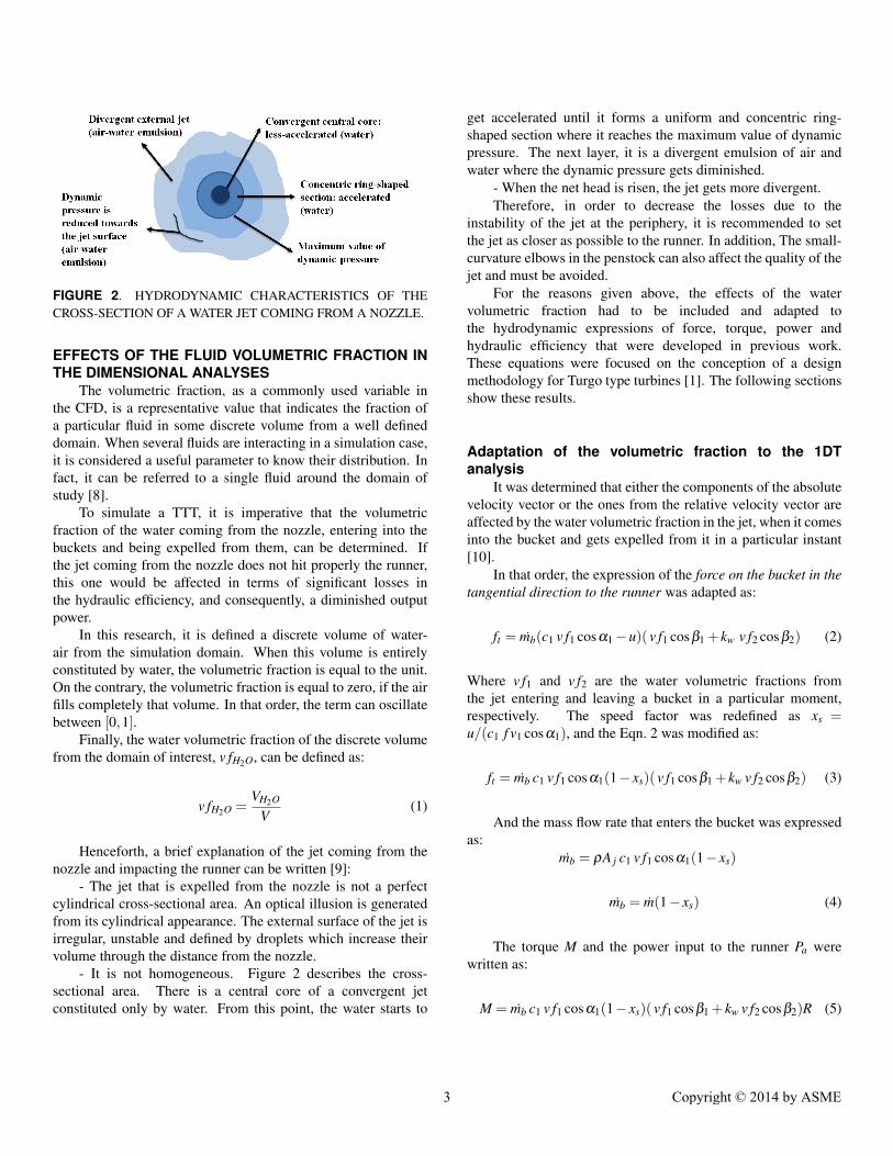
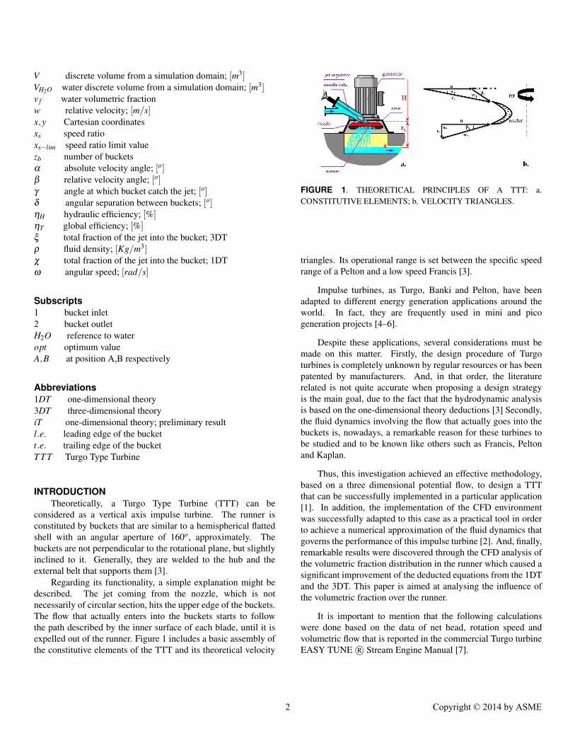
FIGURE 2. HYDRODYNAMIC CHARACTERISTICS OF THECROSS-SECTION OF A WATER JET COMING FROM A NOZZLE.

EFFECTS OF THE FLUID VOLUMETRIC FRACTION INTHE DIMENSIONAL ANALYSES

The volumetric fraction, as a commonly used variable inthe CFD, is a representative value that indicates the fraction ofa particular fluid in some discrete volume from a well defineddomain. When several fluids are interacting in a simulation case,it is considered a useful parameter to know their distribution. Infact, it can be referred to a single fluid around the domain ofstudy [8].

To simulate a TTT, it is imperative that the volumetricfraction of the water coming from the nozzle, entering into thebuckets and being expelled from them, can be determined. Ifthe jet coming from the nozzle does not hit properly the runner,this one would be affected in terms of significant losses inthe hydraulic efficiency, and consequently, a diminished outputpower.

In this research, it is defined a discrete volume of water-air from the simulation domain. When this volume is entirelyconstituted by water, the volumetric fraction is equal to the unit.On the contrary, the volumetric fraction is equal to zero, if the airfills completely that volume. In that order, the term can oscillatebetween [0,1].

Finally, the water volumetric fraction of the discrete volumefrom the domain of interest, v fH2O, can be defined as:

v fH2O =VH2O

V(1)

Henceforth, a brief explanation of the jet coming from thenozzle and impacting the runner can be written [9]:

- The jet that is expelled from the nozzle is not a perfectcylindrical cross-sectional area. An optical illusion is generatedfrom its cylindrical appearance. The external surface of the jet isirregular, unstable and defined by droplets which increase theirvolume through the distance from the nozzle.

- It is not homogeneous. Figure 2 describes the cross-sectional area. There is a central core of a convergent jetconstituted only by water. From this point, the water starts to

get accelerated until it forms a uniform and concentric ring-shaped section where it reaches the maximum value of dynamicpressure. The next layer, it is a divergent emulsion of air andwater where the dynamic pressure gets diminished.

- When the net head is risen, the jet gets more divergent.Therefore, in order to decrease the losses due to the

instability of the jet at the periphery, it is recommended to setthe jet as closer as possible to the runner. In addition, The small-curvature elbows in the penstock can also affect the quality of thejet and must be avoided.

For the reasons given above, the effects of the watervolumetric fraction had to be included and adapted tothe hydrodynamic expressions of force, torque, power andhydraulic efficiency that were developed in previous work.These equations were focused on the conception of a designmethodology for Turgo type turbines [1]. The following sectionsshow these results.

Adaptation of the volumetric fraction to the 1DTanalysis

It was determined that either the components of the absolutevelocity vector or the ones from the relative velocity vector areaffected by the water volumetric fraction in the jet, when it comesinto the bucket and gets expelled from it in a particular instant[10].

In that order, the expression of the force on the bucket in thetangential direction to the runner was adapted as:

ft = mb(c1 v f1 cosα1−u)( v f1 cosβ1 + kw v f2 cosβ2) (2)

Where v f1 and v f2 are the water volumetric fractions fromthe jet entering and leaving a bucket in a particular moment,respectively. The speed factor was redefined as xs =u/(c1 f v1 cosα1), and the Eqn. 2 was modified as:

ft = mb c1 v f1 cosα1(1− xs)( v f1 cosβ1 + kw v f2 cosβ2) (3)

And the mass flow rate that enters the bucket was expressedas:

mb = ρA j c1 v f1 cosα1(1− xs)

mb = m(1− xs) (4)

The torque M and the power input to the runner Pa werewritten as:

M = mb c1 v f1 cosα1(1− xs)( v f1 cosβ1 + kw v f2 cosβ2)R (5)


FIGURE 3. INDICATIVE SCHEME OF THE BUCKETSCATCHING THE JET; A, B AND B´ ARE DIFFERENT POSITIONSOF THE BUCKET.

Pa = mb c21 v f 2

1 cos2α1 xs(1−xs)(v f1 cosβ1 +kw v f2 cosβ2) (6)

While the hydraulic efficiency was determined as:

ηH−iT = 2 v f 21 cos2

α1 xs(1−xs)(v f1 cosβ1 +kw v f2 cosβ2) (7)

It is demonstrable that the hydraulic efficiency from Eqn. 7,reaches its optimum value when xs = 1/2, what led to express uas:

uopt =(c1

2v f1 cosα1

)ηH−iT max

(8)

The jet only does work on the bucket if γ < γlim. It should benoticed that when xs > xs−γlim (see Eqn. 9), the jet hits the rearpart of the precedent bucket.

xs = cos2γlim (9)

Finally, the effects of the water that does not hit the runner mustbe included in the expression of hydraulic efficiency (Eqn. 7):

If xs ≤ xs−lim:

ηH−1DT = ηH−iT χxs≤xs−lim (10)

Where:

χxs≤xs−lim =(γA´+ γB )− xs(tanγA´+ tanγB )

δ(11)

If xs > xs−lim:

ηH−1DT = 2 ηH−iT χxs>xs−lim (12)

Where:

χxs>xs−lim =γA´− xs(tanγA )

δ(13)

And:

xs−lim =2γA−δ

2tanγA(14)

(See Fig. 3)Using:

γA´= γA I f γA ≤ γlim (15)γA´= γlim I f γA > γlim (16)

γB´= γB I f γB ≤ γlim (17)γB´= γlim I f γB > γlim (18)

Adaptation of the volumetric fraction to the 3DTanalysis

A similar adjustment was done for the 3DT case. Thefollowing analysis assumed that the streamlines field in the jetfollows the path described by the jet centreline. It could beexpected for this kind of impulse turbines that even if each part ofthe jet is analysed separately, the resulting average correspondsquite well to the values calculated for the centre element [11,12].

Regarding the components of the forces that hit and leavethe bucket, in the normal direction (see Fig. 4.b); it was assumedthat the deviation angle at the entry while the runner rotates isthe same at the exit, ν = ν1 = ν2 (this is probably true only at thecentre of the bucket) This can be expressed as:

Ft1−3DT = mb w1 v f1 cosβ1 cosν (19)Ft2−3DT = mb w2 v f2 cosβ2 cosν (20)

The power output from the runner, P3DT (Eqn. 21), whichwas deduced in previous work [1], was redefined to includethe effects at the inlet and outlet of the jet from the bucket, asfollows:

Pb−3DT = mb w1 vt cosν ( v f1 cosβ1 + kw v f2 cosβ2) (21)


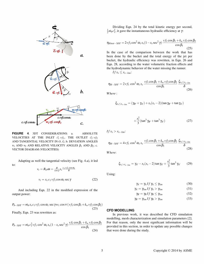
FIGURE 4. 3DT CONSIDERATIONS: a. ABSOLUTEVELOCITIES AT THE INLET ~c1 v f1, THE OUTLET ~c2 v f2AND TANGENTIAL VELOCITY IN O, ~vt ; b. DEVIATION ANGLESν1 AND ν2 AND RELATIVE VELOCITY ANGLES β1 AND β2; c.VECTOR DIAGRAM (VELOCITIES)

Adapting as well the tangential velocity (see Fig. 4.a), it ledto:

vt = ROω = Rcosγ

xsc1 v f1 cosα1

R

vt = xs c1 v f1 cosα1 secγ (22)

And including Eqn. 22 in the modified expression of theoutput power:

Pb−3DT = mb xs c1 v f1 cosα1 secγ w1 cosν (v f1 cosβ1+kw v f2 cosβ2)(23)

Finally, Eqn. 23 was rewritten as:

Pb−3DT = mb c21 v f1 cos2

α1 xs(1−xs sec2γ)

v f1 cosβ1 + kw v f2 cosβ2

cosβ1(24)

Dividing Eqn. 24 by the total kinetic energy per second,12 mbc2

1, it gave the instantaneous hydraulic efficiency at γ:

ηHinst−3DT = 2v f1 cos2α1 xs(1−xs sec2

γ)v f1 cosβ1 + kw v f2 cosβ2

cosβ1(25)

In the case of the comparison between the work that hasbeen done by the bucket and the total energy of the jet perbucket, the hydraulic efficiency was rewritten, in Eqn. 26 andEqn. 28, according to the water volumetric fraction effects andthe hydrodynamic behavior of the water missing the runner.

I f xs ≤ xs−lim:

ηH−3DT = 2 v f1 cos2α1 xs


cosβ1

ξxs≤xs−lim

δ

(26)Where :

ξxs≤xs−lim = (γB′ + γA′)+ xs(xs−2)(tanγB′ + tanγA′)

+x2

s

3(tan3

γB′ + tan3γA′) (27)

I f xs > xs−lim:

ηH−3DT = 4 v f1 cos2α1 xs


cosβ1

ξxs>xs−lim

δ

(28)Where:

ξxs>xs−lim = γA′ − xs(xs−2) tanγA′ +x2

s

3tan3

γA′ (29)

Using:

γA´= γA I f γA ≤ γlim (30)γA´= γlim I f γA > γlim (31)

γB´= γB I f γB ≤ γlim (32)γB´= γlim I f γB > γlim (33)

CFD MODELLINGIn previous work, it was described the CFD simulation

modelling, mesh characterization and simulation parameters [2].For that reason, only the most significant information will beprovided in this section, in order to update any possible changesthat were done during the study.


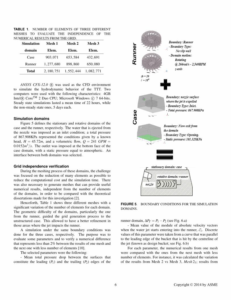
TABLE 1. NUMBER OF ELEMENTS OF THREE DIFFERENTMESHES TO EVALUATE THE INDEPENDENCE OF THENUMERICAL RESULTS FROM THE GRID.

Simulation Mesh 1 Mesh 2 Mesh 3

domain Elem. Elem. Elem.

Case 903,071 653,584 432,691

Runner 1,277,680 898,860 650,080

Total 2,180,751 1,552,444 1,082,771

ANSYS CFX-12.0 R© was used as the CFD environmentto simulate the hydrodynamic behavior of the TTT. Twocomputers were used with the following characteristics: 4GBIntel R© CoreTM 2 Duo CPU; Microsoft Windows c© 7 64-bits.Steady state simulations lasted a mean time of 22 hours, whilethe non-steady state ones, 5 days each.

Simulation domainsFigure 5 defines the stationary and rotative domains of the

case and the runner, respectively. The water that is ejected fromthe nozzle was imposed as an inlet condition; a total pressureof 867.908KPa represented the conditions given by a knownhead, H = 45.72m, and a volumetric flow, Q = 241 GPM =0.0152m3/s. The outlet was imposed at the bottom face of thecase domain, with a static pressure equal to atmospheric. Aninterface between both domains was selected.

Grid independence verificationDuring the meshing process of these domains, the challenge

was focused on the reduction of many elements as possible toreduce the computational cost and the simulation time. Therewas also necessary to generate meshes that can provide usefulnumerical results, independent from the number of elementsof the domains, in order to be compared with the theoreticaldissertations made for this investigation [2].

Henceforth, Table 1 shows three different meshes with asignificant variation of the number of elements for each domain.The geometric difficulty of the domains, particularly the onefrom the runner, guided the grid generation process to theunstructured case. This allowed to have a better refinement inthose areas where the jet impacts the runner.

A simulation under the same boundary conditions wasdone for the three cases, respectively. The purpose was toevaluate some parameters and to verify a numerical differencethat represents less than 2% between the results of one mesh andthe next one with less number of elements [10].

The selected parameters were the following:- Mean total pressure drop between the surfaces that

constitute the leading (P1) and the trailing (P2) edges of the

FIGURE 5. BOUNDARY CONDITIONS FOR THE SIMULATIONDOMAINS.

runner domain, ∆PT = P1−P2 (see Fig. 6.a)- Mean value of the module of absolute velocity vectors

when the water jet starts entering into the runner, ~c1. Discretevalues of this parameter were taken from a curve that was parallelto the leading edge of the bucket that is hit by the centreline ofthe jet (known as design bucket; see Fig. 6.b)

For each parameter, the numerical results from one meshwere compared with the ones from the next mesh with lessnumber of elements. For instance, it was calculated the variationof the results from Mesh 2 vs Mesh 3, Mesh 23; results from


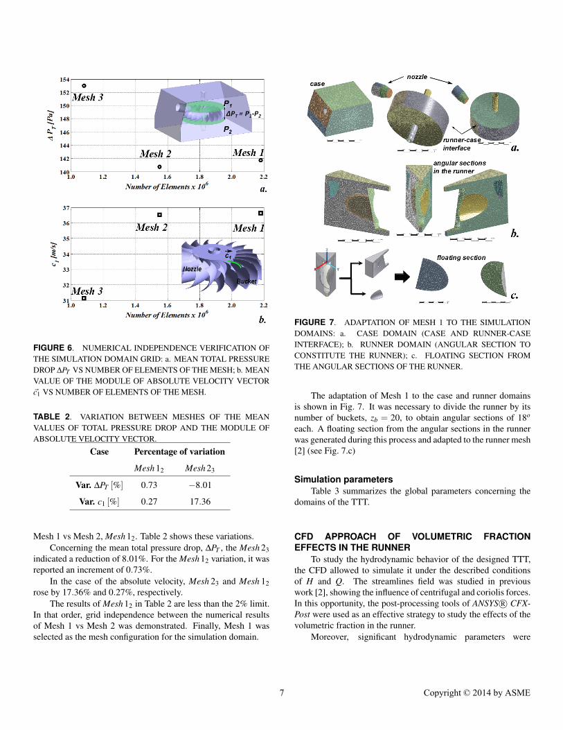
FIGURE 6. NUMERICAL INDEPENDENCE VERIFICATION OFTHE SIMULATION DOMAIN GRID: a. MEAN TOTAL PRESSUREDROP ∆PT VS NUMBER OF ELEMENTS OF THE MESH; b. MEANVALUE OF THE MODULE OF ABSOLUTE VELOCITY VECTOR~c1 VS NUMBER OF ELEMENTS OF THE MESH.

TABLE 2. VARIATION BETWEEN MESHES OF THE MEANVALUES OF TOTAL PRESSURE DROP AND THE MODULE OFABSOLUTE VELOCITY VECTOR.

Case Percentage of variation

Mesh 12 Mesh 23

Var. ∆PT [%] 0.73 −8.01

Var. c1 [%] 0.27 17.36

Mesh 1 vs Mesh 2, Mesh 12. Table 2 shows these variations.Concerning the mean total pressure drop, ∆PT , the Mesh 23

indicated a reduction of 8.01%. For the Mesh 12 variation, it wasreported an increment of 0.73%.

In the case of the absolute velocity, Mesh 23 and Mesh 12rose by 17.36% and 0.27%, respectively.

The results of Mesh 12 in Table 2 are less than the 2% limit.In that order, grid independence between the numerical resultsof Mesh 1 vs Mesh 2 was demonstrated. Finally, Mesh 1 wasselected as the mesh configuration for the simulation domain.

FIGURE 7. ADAPTATION OF MESH 1 TO THE SIMULATIONDOMAINS: a. CASE DOMAIN (CASE AND RUNNER-CASEINTERFACE); b. RUNNER DOMAIN (ANGULAR SECTION TOCONSTITUTE THE RUNNER); c. FLOATING SECTION FROMTHE ANGULAR SECTIONS OF THE RUNNER.

The adaptation of Mesh 1 to the case and runner domainsis shown in Fig. 7. It was necessary to divide the runner by itsnumber of buckets, zb = 20, to obtain angular sections of 18o

each. A floating section from the angular sections in the runnerwas generated during this process and adapted to the runner mesh[2] (see Fig. 7.c)

Simulation parametersTable 3 summarizes the global parameters concerning the

domains of the TTT.

CFD APPROACH OF VOLUMETRIC FRACTIONEFFECTS IN THE RUNNER

To study the hydrodynamic behavior of the designed TTT,the CFD allowed to simulate it under the described conditionsof H and Q. The streamlines field was studied in previouswork [2], showing the influence of centrifugal and coriolis forces.In this opportunity, the post-processing tools of ANSYS R© CFX-Post were used as an effective strategy to study the effects of thevolumetric fraction in the runner.

Moreover, significant hydrodynamic parameters were


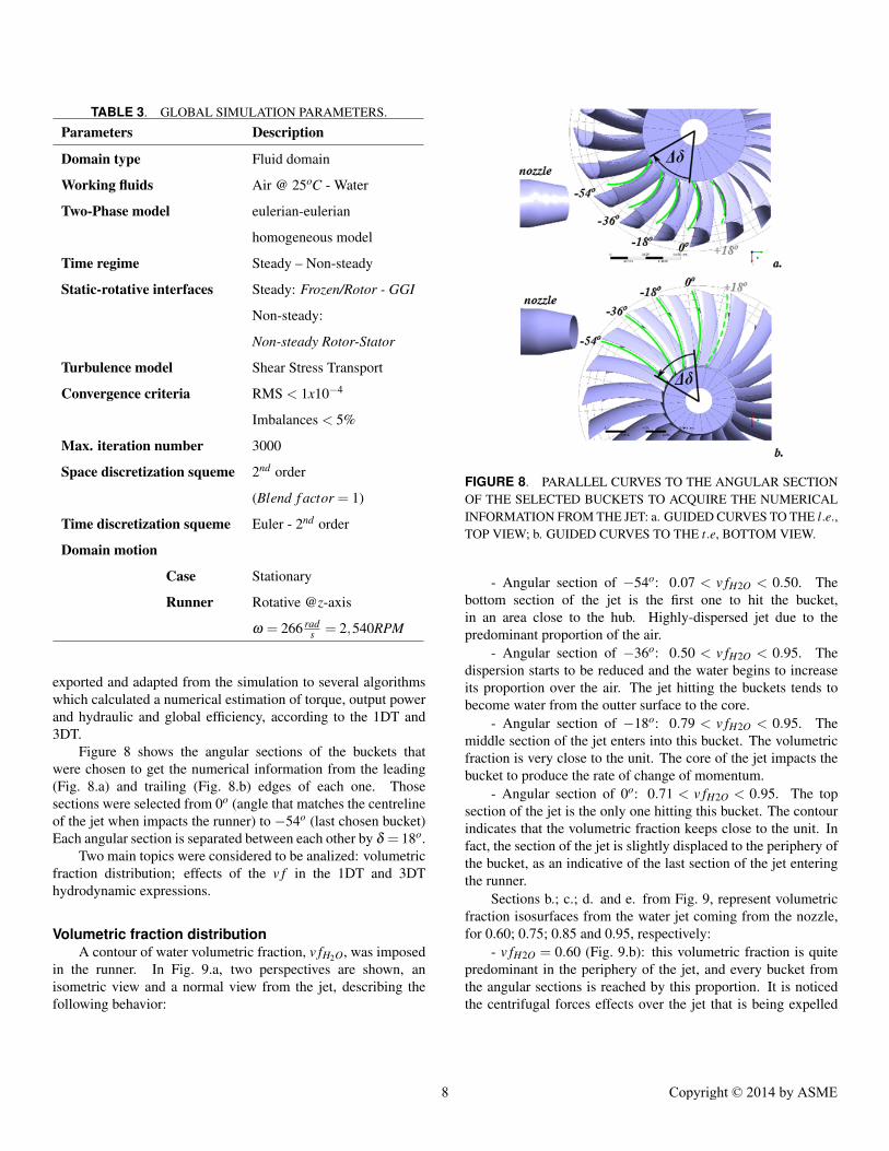
TABLE 3. GLOBAL SIMULATION PARAMETERS.

Parameters Description

Domain type Fluid domain

Working fluids Air @ 25oC - Water

Two-Phase model eulerian-eulerian

homogeneous model

Time regime Steady – Non-steady

Static-rotative interfaces Steady: Frozen/Rotor - GGI

Non-steady:

Non-steady Rotor-Stator

Turbulence model Shear Stress Transport

Convergence criteria RMS < 1x10−4

Imbalances < 5%

Max. iteration number 3000

Space discretization squeme 2nd order

(Blend f actor = 1)

Time discretization squeme Euler - 2nd order

Domain motion

Case Stationary

Runner Rotative @z-axis

ω = 266 rads = 2,540RPM

exported and adapted from the simulation to several algorithmswhich calculated a numerical estimation of torque, output powerand hydraulic and global efficiency, according to the 1DT and3DT.

Figure 8 shows the angular sections of the buckets thatwere chosen to get the numerical information from the leading(Fig. 8.a) and trailing (Fig. 8.b) edges of each one. Thosesections were selected from 0o (angle that matches the centrelineof the jet when impacts the runner) to −54o (last chosen bucket)Each angular section is separated between each other by δ = 18o.

Two main topics were considered to be analized: volumetricfraction distribution; effects of the v f in the 1DT and 3DThydrodynamic expressions.

Volumetric fraction distributionA contour of water volumetric fraction, v fH2O, was imposed

in the runner. In Fig. 9.a, two perspectives are shown, anisometric view and a normal view from the jet, describing thefollowing behavior:

FIGURE 8. PARALLEL CURVES TO THE ANGULAR SECTIONOF THE SELECTED BUCKETS TO ACQUIRE THE NUMERICALINFORMATION FROM THE JET: a. GUIDED CURVES TO THE l.e.,TOP VIEW; b. GUIDED CURVES TO THE t.e, BOTTOM VIEW.

- Angular section of −54o: 0.07 < v fH2O < 0.50. Thebottom section of the jet is the first one to hit the bucket,in an area close to the hub. Highly-dispersed jet due to thepredominant proportion of the air.

- Angular section of −36o: 0.50 < v fH2O < 0.95. Thedispersion starts to be reduced and the water begins to increaseits proportion over the air. The jet hitting the buckets tends tobecome water from the outter surface to the core.

- Angular section of −18o: 0.79 < v fH2O < 0.95. Themiddle section of the jet enters into this bucket. The volumetricfraction is very close to the unit. The core of the jet impacts thebucket to produce the rate of change of momentum.

- Angular section of 0o: 0.71 < v fH2O < 0.95. The topsection of the jet is the only one hitting this bucket. The contourindicates that the volumetric fraction keeps close to the unit. Infact, the section of the jet is slightly displaced to the periphery ofthe bucket, as an indicative of the last section of the jet enteringthe runner.

Sections b.; c.; d. and e. from Fig. 9, represent volumetricfraction isosurfaces from the water jet coming from the nozzle,for 0.60; 0.75; 0.85 and 0.95, respectively:

- v fH2O = 0.60 (Fig. 9.b): this volumetric fraction is quitepredominant in the periphery of the jet, and every bucket fromthe angular sections is reached by this proportion. It is noticedthe centrifugal forces effects over the jet that is being expelled


FIGURE 9. VOLUMETRIC FRACTION DISTRIBUTION OF THEWATER, CONTOURS AND ISOSURFACES: a. ISOSURFACE OFv fH2O = 0.00; b. ISOSURFACE OF v fH2O = 0.60; c. ISOSURFACEOF v fH2O = 0.75; d. ISOSURFACE OF v fH2O = 0.85; e.ISOSURFACE OF v fH2O = 0.95.

from the runner through the trailing edge.- v fH2O = 0.75 (Fig. 9.c): the jet tends to converge to its

centreline as the volumetric fraction gets closer to the unit. Onlythe angular sections from 0o to −36o are being impacted by thisvalue.

- v fH2O = 0.85 (Fig. 9.d): the normal view from the nozzleshows the jet tendency to follow its centreline through the bucket,which was predicted by the dimensional analysis methodology.Angular sections from 0o to −18o receive the greatest portion ofthe jet at this volumetric fraction.

- v fH2O = 0.95 (Fig. 9.e): the proximity of the jet to itsconvergent central core is totally defined for this volumetric

fraction isosurface. As this fraction is close to the unit, thejet, which corresponds to the one from the centreline, enters therunner through the angular section of 0o. This is completelyexpected by the design methodology. A very little section ofthe jet comes into the angular section at −180, and a similar oneexceeds the bucket at 0o.

In this way, the study of the jet that enters the runner allowedto confirm the condition of a water-air emulsion in the runner,which is unstable and non-homogeneous. While the cross-sectional area of the jet clearly differed from a perfect cylinder.The hydrodynamics of the jet crossing the runner was clearlyaffected by this behavior.

Torque, power and efficiencyDimensional analysis equations from 1DT and 3DT were

numerically estimated from a steady state CFD simulation, anda comparison with the equations which do not include thevolumetric fraction effects [1] was done. A range between0.60 < v fH2O < 1.00 was selected as a significant range in whichthe jet can transfer the energy to the runner. Through Fig. 10 andFig. 11, it was possible to conclude about the water volumetricfraction and its impact over the torque (Eqn. 5), the power(Eqn. 6) and the efficiency (Eqn. 10 and Eqn. 26) in the TTTrunner. There were significant results referred to the angularsections in the runner, that needed to be mentioned:

- Torque, Mz−T 1D and Power, Pa−T 1D: From Fig. 10.a,b (nov f effects included), bucket at −54o showed a peak value of0.5N.m / 125W , very close to the hub region. A similar peakappeared at−36o, however, it began to move away from the hub,and the torque and power distributions were sustained between1.6 < x/d < 2.4. Bucket at −18o reported two peaks of 0.6N.m/ 150W , approximately, and a slight depression in the centrelineregion of 0.4N.m / 7,000W : this bucket generated the maximumtorque and power, indicating that an important fraction of the jeteffectively transferred its energy to this bucket. Last fraction ofthe jet at 0o showed the same behavior as −18o but in a smallerregion between 1.6 < x/d < 2.6; maximum torque and power of0.4N.m / 100W .

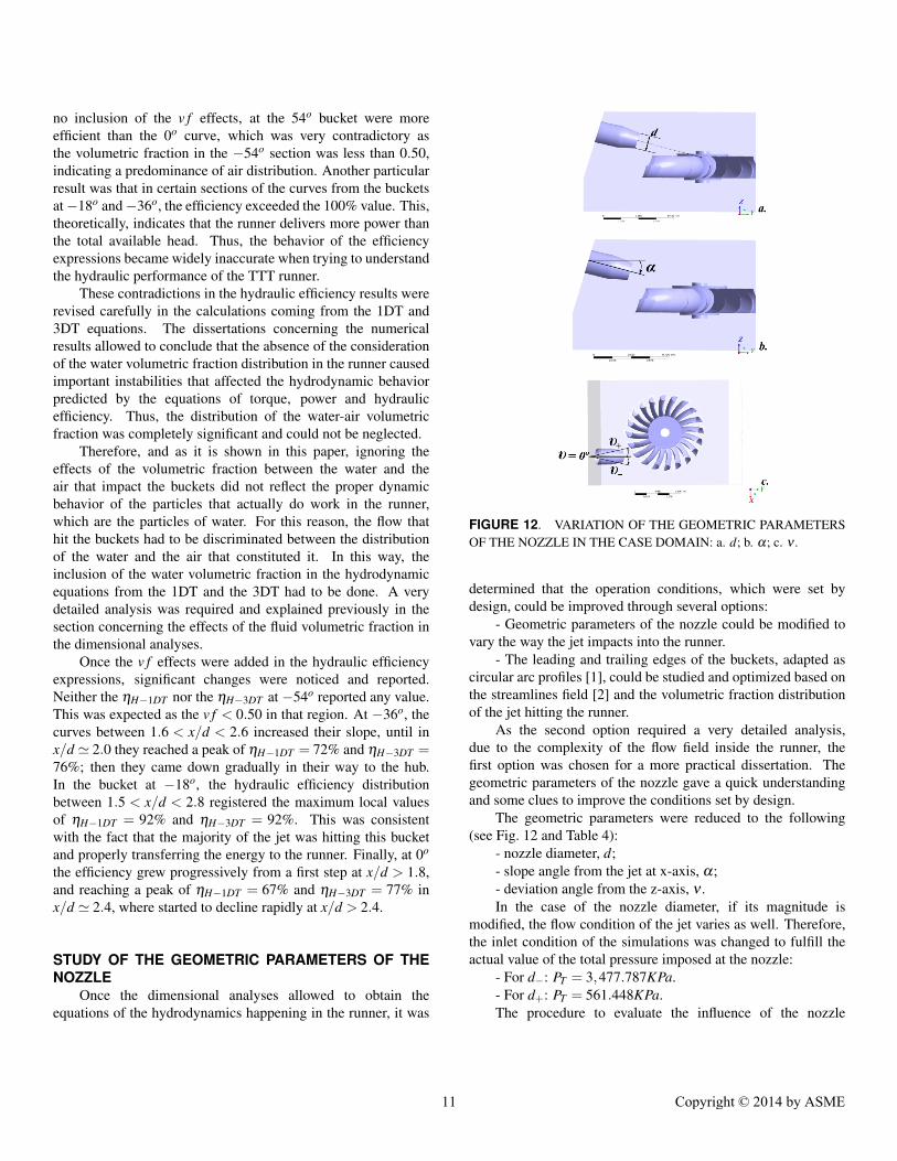
In sharp contrast to the previous analysis, the inclusion of thev f effects changed the torque and power distributions through thebuckets (Fig. 11.a,b) Bucket at −54o did not report a significantcontribution to the torque and the power. In the case at −36o,a peak of 0.5N.m / 140W appeared between 1.8 < x/d < 2.4,and gradually disminished to the extremes of the range. Thebucket at −18o, for the same x/d range, reached a very stablevalues of 0.6N.m / 160W , being the highest values reported; thissection received most of the jet from the nozzle, as it happened inFig. 10.a,b. The 0o section differed from the previous describedbehavior, announcing that the last fraction of the jet is enteringthe runner; its maximum value almost hit the 0.5N.m / 125Wlimit, then it was reduced to 0.2N.m / 50W between 1.8 < x/d <


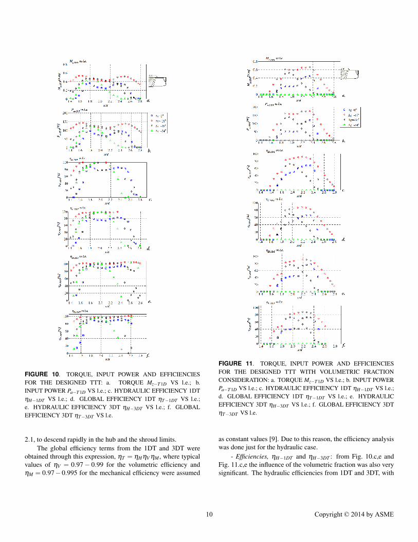
FIGURE 10. TORQUE, INPUT POWER AND EFFICIENCIESFOR THE DESIGNED TTT: a. TORQUE Mz−T 1D VS l.e.; b.INPUT POWER Pa−T 1D VS l.e.; c. HYDRAULIC EFFICIENCY 1DTηH−1DT VS l.e.; d. GLOBAL EFFICIENCY 1DT ηT−1DT VS l.e.;e. HYDRAULIC EFFICIENCY 3DT ηH−3DT VS l.e.; f. GLOBALEFFICIENCY 3DT ηT−3DT VS l.e.

2.1, to descend rapidly in the hub and the shroud limits.The global efficiency terms from the 1DT and 3DT were

obtained through this expression, ηT = ηHηV ηM , where typicalvalues of ηV = 0.97− 0.99 for the volumetric efficiency andηM = 0.97− 0.995 for the mechanical efficiency were assumed

FIGURE 11. TORQUE, INPUT POWER AND EFFICIENCIESFOR THE DESIGNED TTT WITH VOLUMETRIC FRACTIONCONSIDERATION: a. TORQUE Mz−T 1D VS l.e.; b. INPUT POWERPa−T 1D VS l.e.; c. HYDRAULIC EFFICIENCY 1DT ηH−1DT VS l.e.;d. GLOBAL EFFICIENCY 1DT ηT−1DT VS l.e.; e. HYDRAULICEFFICIENCY 3DT ηH−3DT VS l.e.; f. GLOBAL EFFICIENCY 3DTηT−3DT VS l.e.

as constant values [9]. Due to this reason, the efficiency analysiswas done just for the hydraulic case.

- Efficiencies, ηH−1DT and ηH−3DT : from Fig. 10.c,e andFig. 11.c,e the influence of the volumetric fraction was also verysignificant. The hydraulic efficiencies from 1DT and 3DT, with


no inclusion of the v f effects, at the 54o bucket were moreefficient than the 0o curve, which was very contradictory asthe volumetric fraction in the −54o section was less than 0.50,indicating a predominance of air distribution. Another particularresult was that in certain sections of the curves from the bucketsat−18o and−36o, the efficiency exceeded the 100% value. This,theoretically, indicates that the runner delivers more power thanthe total available head. Thus, the behavior of the efficiencyexpressions became widely inaccurate when trying to understandthe hydraulic performance of the TTT runner.

These contradictions in the hydraulic efficiency results wererevised carefully in the calculations coming from the 1DT and3DT equations. The dissertations concerning the numericalresults allowed to conclude that the absence of the considerationof the water volumetric fraction distribution in the runner causedimportant instabilities that affected the hydrodynamic behaviorpredicted by the equations of torque, power and hydraulicefficiency. Thus, the distribution of the water-air volumetricfraction was completely significant and could not be neglected.

Therefore, and as it is shown in this paper, ignoring theeffects of the volumetric fraction between the water and theair that impact the buckets did not reflect the proper dynamicbehavior of the particles that actually do work in the runner,which are the particles of water. For this reason, the flow thathit the buckets had to be discriminated between the distributionof the water and the air that constituted it. In this way, theinclusion of the water volumetric fraction in the hydrodynamicequations from the 1DT and the 3DT had to be done. A verydetailed analysis was required and explained previously in thesection concerning the effects of the fluid volumetric fraction inthe dimensional analyses.

Once the v f effects were added in the hydraulic efficiencyexpressions, significant changes were noticed and reported.Neither the ηH−1DT nor the ηH−3DT at −54o reported any value.This was expected as the v f < 0.50 in that region. At −36o, thecurves between 1.6 < x/d < 2.6 increased their slope, until inx/d ' 2.0 they reached a peak of ηH−1DT = 72% and ηH−3DT =76%; then they came down gradually in their way to the hub.In the bucket at −18o, the hydraulic efficiency distributionbetween 1.5 < x/d < 2.8 registered the maximum local valuesof ηH−1DT = 92% and ηH−3DT = 92%. This was consistentwith the fact that the majority of the jet was hitting this bucketand properly transferring the energy to the runner. Finally, at 0o

the efficiency grew progressively from a first step at x/d > 1.8,and reaching a peak of ηH−1DT = 67% and ηH−3DT = 77% inx/d ' 2.4, where started to decline rapidly at x/d > 2.4.

STUDY OF THE GEOMETRIC PARAMETERS OF THENOZZLE

Once the dimensional analyses allowed to obtain theequations of the hydrodynamics happening in the runner, it was

FIGURE 12. VARIATION OF THE GEOMETRIC PARAMETERSOF THE NOZZLE IN THE CASE DOMAIN: a. d; b. α; c. ν .

determined that the operation conditions, which were set bydesign, could be improved through several options:

- Geometric parameters of the nozzle could be modified tovary the way the jet impacts into the runner.

- The leading and trailing edges of the buckets, adapted ascircular arc profiles [1], could be studied and optimized based onthe streamlines field [2] and the volumetric fraction distributionof the jet hitting the runner.

As the second option required a very detailed analysis,due to the complexity of the flow field inside the runner, thefirst option was chosen for a more practical dissertation. Thegeometric parameters of the nozzle gave a quick understandingand some clues to improve the conditions set by design.

The geometric parameters were reduced to the following(see Fig. 12 and Table 4):

- nozzle diameter, d;- slope angle from the jet at x-axis, α;- deviation angle from the z-axis, ν .In the case of the nozzle diameter, if its magnitude is

modified, the flow condition of the jet varies as well. Therefore,the inlet condition of the simulations was changed to fulfill theactual value of the total pressure imposed at the nozzle:

- For d−: PT = 3,477.787KPa.- For d+: PT = 561.448KPa.The procedure to evaluate the influence of the nozzle


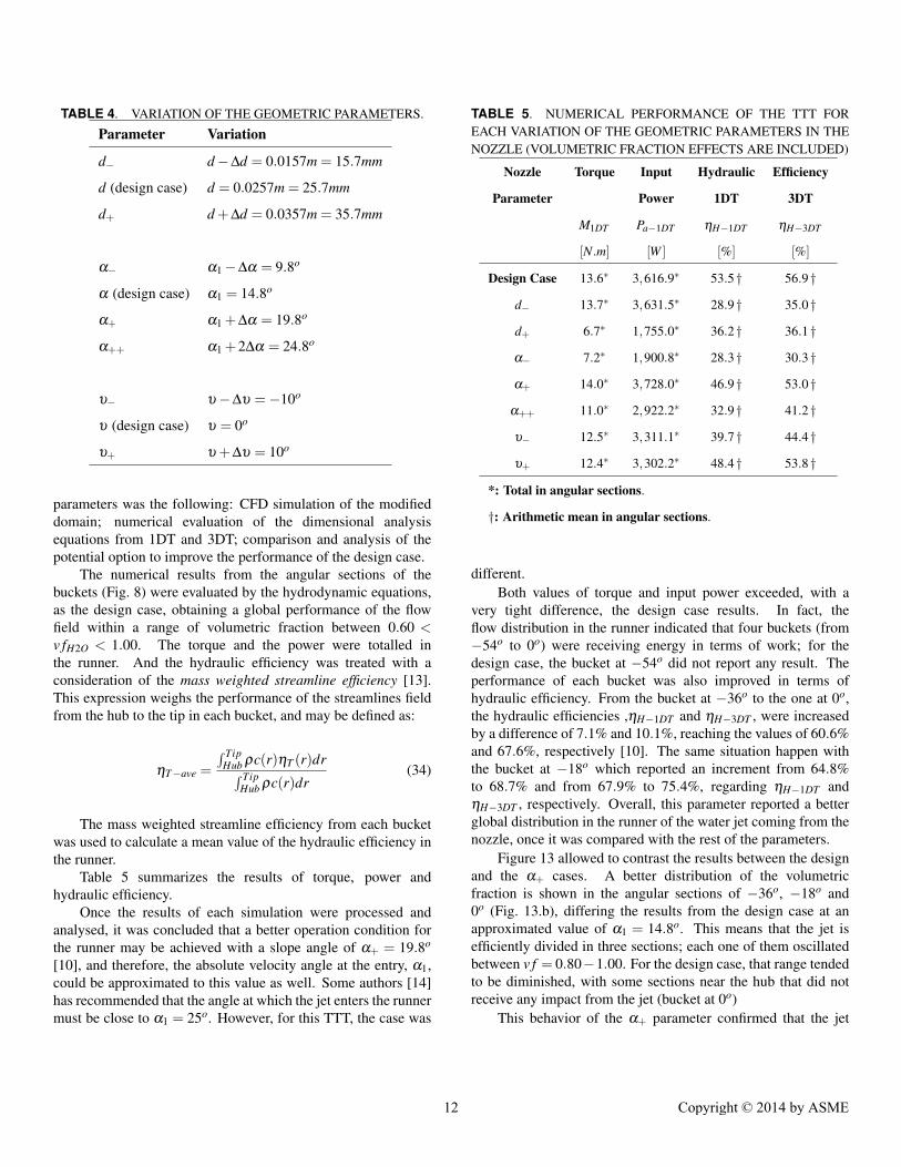
TABLE 4. VARIATION OF THE GEOMETRIC PARAMETERS.

Parameter Variation

d− d−∆d = 0.0157m = 15.7mm

d (design case) d = 0.0257m = 25.7mm

d+ d +∆d = 0.0357m = 35.7mm

α− α1−∆α = 9.8o

α (design case) α1 = 14.8o

α+ α1 +∆α = 19.8o

α++ α1 +2∆α = 24.8o

υ− υ−∆υ =−10o

υ (design case) υ = 0o

υ+ υ +∆υ = 10o

parameters was the following: CFD simulation of the modifieddomain; numerical evaluation of the dimensional analysisequations from 1DT and 3DT; comparison and analysis of thepotential option to improve the performance of the design case.

The numerical results from the angular sections of thebuckets (Fig. 8) were evaluated by the hydrodynamic equations,as the design case, obtaining a global performance of the flowfield within a range of volumetric fraction between 0.60 <v fH2O < 1.00. The torque and the power were totalled inthe runner. And the hydraulic efficiency was treated with aconsideration of the mass weighted streamline efficiency [13].This expression weighs the performance of the streamlines fieldfrom the hub to the tip in each bucket, and may be defined as:

ηT−ave =

∫ TipHub ρc(r)ηT (r)dr∫ Tip

Hub ρc(r)dr(34)

The mass weighted streamline efficiency from each bucketwas used to calculate a mean value of the hydraulic efficiency inthe runner.

Table 5 summarizes the results of torque, power andhydraulic efficiency.

Once the results of each simulation were processed andanalysed, it was concluded that a better operation condition forthe runner may be achieved with a slope angle of α+ = 19.8o

[10], and therefore, the absolute velocity angle at the entry, α1,could be approximated to this value as well. Some authors [14]has recommended that the angle at which the jet enters the runnermust be close to α1 = 25o. However, for this TTT, the case was

TABLE 5. NUMERICAL PERFORMANCE OF THE TTT FOREACH VARIATION OF THE GEOMETRIC PARAMETERS IN THENOZZLE (VOLUMETRIC FRACTION EFFECTS ARE INCLUDED)

Nozzle Torque Input Hydraulic Efficiency

Parameter Power 1DT 3DT

M1DT Pa−1DT ηH−1DT ηH−3DT

[N.m] [W ] [%] [%]

Design Case 13.6∗ 3,616.9∗ 53.5 † 56.9 †

d− 13.7∗ 3,631.5∗ 28.9 † 35.0 †

d+ 6.7∗ 1,755.0∗ 36.2 † 36.1 †

α− 7.2∗ 1,900.8∗ 28.3 † 30.3 †

α+ 14.0∗ 3,728.0∗ 46.9 † 53.0 †

α++ 11.0∗ 2,922.2∗ 32.9 † 41.2 †

υ− 12.5∗ 3,311.1∗ 39.7 † 44.4 †

υ+ 12.4∗ 3,302.2∗ 48.4 † 53.8 †

*: Total in angular sections.

†: Arithmetic mean in angular sections.

different.Both values of torque and input power exceeded, with a

very tight difference, the design case results. In fact, theflow distribution in the runner indicated that four buckets (from−54o to 0o) were receiving energy in terms of work; for thedesign case, the bucket at −54o did not report any result. Theperformance of each bucket was also improved in terms ofhydraulic efficiency. From the bucket at −36o to the one at 0o,the hydraulic efficiencies ,ηH−1DT and ηH−3DT , were increasedby a difference of 7.1% and 10.1%, reaching the values of 60.6%and 67.6%, respectively [10]. The same situation happen withthe bucket at −18o which reported an increment from 64.8%to 68.7% and from 67.9% to 75.4%, regarding ηH−1DT andηH−3DT , respectively. Overall, this parameter reported a betterglobal distribution in the runner of the water jet coming from thenozzle, once it was compared with the rest of the parameters.

Figure 13 allowed to contrast the results between the designand the α+ cases. A better distribution of the volumetricfraction is shown in the angular sections of −36o, −18o and0o (Fig. 13.b), differing the results from the design case at anapproximated value of α1 = 14.8o. This means that the jet isefficiently divided in three sections; each one of them oscillatedbetween v f = 0.80−1.00. For the design case, that range tendedto be diminished, with some sections near the hub that did notreceive any impact from the jet (bucket at 0o)

This behavior of the α+ parameter confirmed that the jet


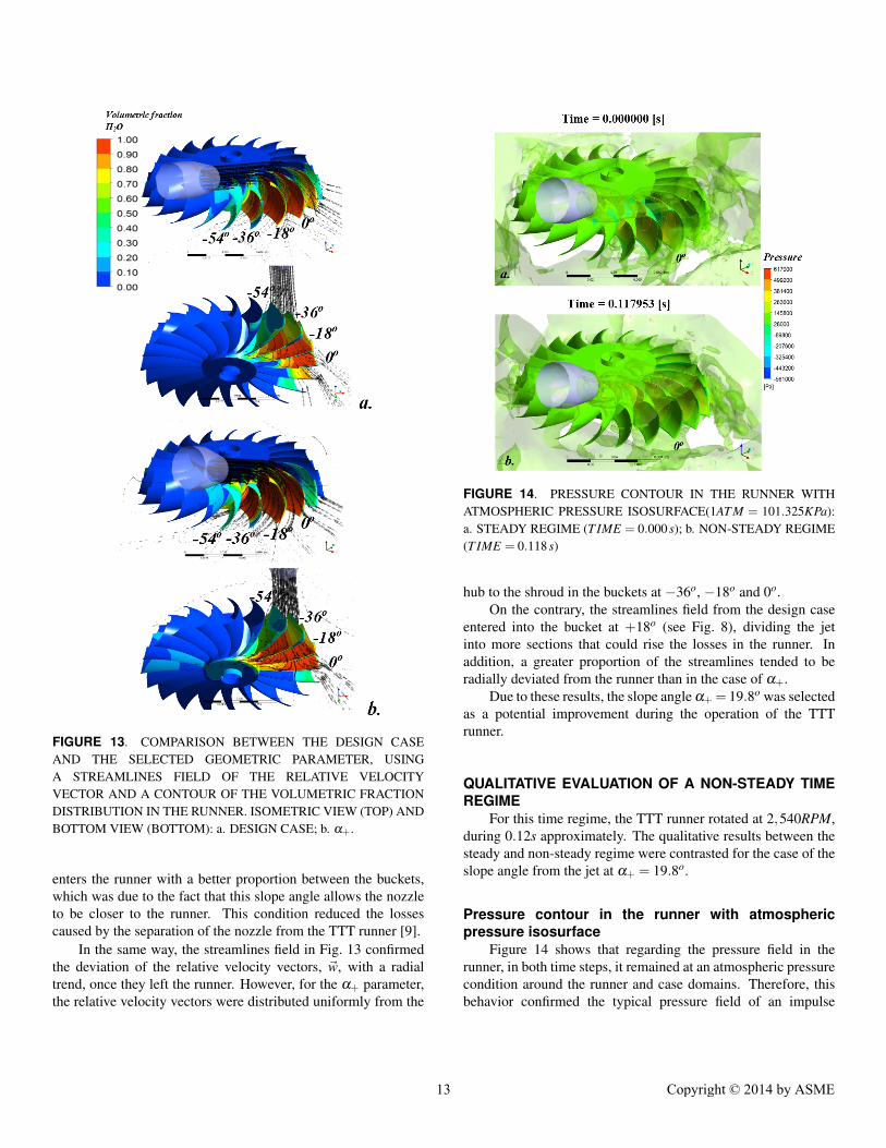
FIGURE 13. COMPARISON BETWEEN THE DESIGN CASEAND THE SELECTED GEOMETRIC PARAMETER, USINGA STREAMLINES FIELD OF THE RELATIVE VELOCITYVECTOR AND A CONTOUR OF THE VOLUMETRIC FRACTIONDISTRIBUTION IN THE RUNNER. ISOMETRIC VIEW (TOP) ANDBOTTOM VIEW (BOTTOM): a. DESIGN CASE; b. α+.

enters the runner with a better proportion between the buckets,which was due to the fact that this slope angle allows the nozzleto be closer to the runner. This condition reduced the lossescaused by the separation of the nozzle from the TTT runner [9].

In the same way, the streamlines field in Fig. 13 confirmedthe deviation of the relative velocity vectors, ~w, with a radialtrend, once they left the runner. However, for the α+ parameter,the relative velocity vectors were distributed uniformly from the

FIGURE 14. PRESSURE CONTOUR IN THE RUNNER WITHATMOSPHERIC PRESSURE ISOSURFACE(1AT M = 101.325KPa):a. STEADY REGIME (T IME = 0.000 s); b. NON-STEADY REGIME(T IME = 0.118 s)

hub to the shroud in the buckets at −36o, −18o and 0o.On the contrary, the streamlines field from the design case

entered into the bucket at +18o (see Fig. 8), dividing the jetinto more sections that could rise the losses in the runner. Inaddition, a greater proportion of the streamlines tended to beradially deviated from the runner than in the case of α+.

Due to these results, the slope angle α+ = 19.8o was selectedas a potential improvement during the operation of the TTTrunner.

QUALITATIVE EVALUATION OF A NON-STEADY TIMEREGIME

For this time regime, the TTT runner rotated at 2,540RPM,during 0.12s approximately. The qualitative results between thesteady and non-steady regime were contrasted for the case of theslope angle from the jet at α+ = 19.8o.

Pressure contour in the runner with atmosphericpressure isosurface

Figure 14 shows that regarding the pressure field in therunner, in both time steps, it remained at an atmospheric pressurecondition around the runner and case domains. Therefore, thisbehavior confirmed the typical pressure field of an impulse


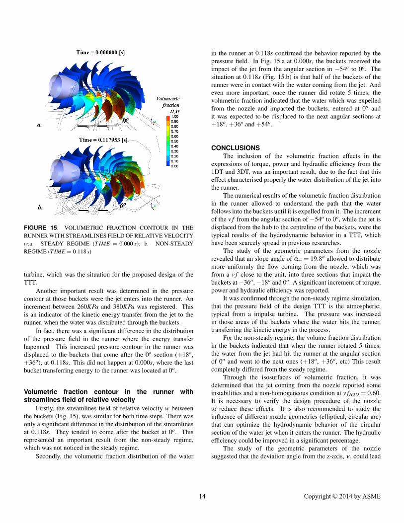
FIGURE 15. VOLUMETRIC FRACTION CONTOUR IN THERUNNER WITH STREAMLINES FIELD OF RELATIVE VELOCITYw:a. STEADY REGIME (T IME = 0.000 s); b. NON-STEADYREGIME (T IME = 0.118 s)

turbine, which was the situation for the proposed design of theTTT.

Another important result was determined in the pressurecontour at those buckets were the jet enters into the runner. Anincrement between 260KPa and 380KPa was registered. Thisis an indicator of the kinetic energy transfer from the jet to therunner, when the water was distributed through the buckets.

In fact, there was a significant difference in the distributionof the pressure field in the runner where the energy transferhapenned. This increased pressure contour in the runner wasdisplaced to the buckets that come after the 0o section (+18o,+36o), at 0.118s. This did not happen at 0.000s, where the lastbucket transferring energy to the runner was located at 0o.

Volumetric fraction contour in the runner withstreamlines field of relative velocity

Firstly, the streamlines field of relative velocity w betweenthe buckets (Fig. 15), was similar for both time steps. There wasonly a significant difference in the distribution of the streamlinesat 0.118s. They tended to come after the bucket at 0o. Thisrepresented an important result from the non-steady regime,which was not noticed in the steady regime.

Secondly, the volumetric fraction distribution of the water

in the runner at 0.118s confirmed the behavior reported by thepressure field. In Fig. 15.a at 0.000s, the buckets received theimpact of the jet from the angular section in −54o to 0o. Thesituation at 0.118s (Fig. 15.b) is that half of the buckets of therunner were in contact with the water coming from the jet. Andeven more important, once the runner did rotate 5 times, thevolumetric fraction indicated that the water which was expelledfrom the nozzle and impacted the buckets, entered at 0o andit was expected to be displaced to the next angular sections at+18o, +36o and +54o.

CONCLUSIONSThe inclusion of the volumetric fraction effects in the

expressions of torque, power and hydraulic efficiency from the1DT and 3DT, was an important result, due to the fact that thiseffect characterised properly the water distribution of the jet intothe runner.

The numerical results of the volumetric fraction distributionin the runner allowed to understand the path that the waterfollows into the buckets until it is expelled from it. The incrementof the v f from the angular section of −54o to 0o, while the jet isdisplaced from the hub to the centreline of the buckets, were thetypical results of the hydrodynamic behavior in a TTT, whichhave been scarcely spread in previous researches.

The study of the geometric parameters from the nozzlerevealed that an slope angle of α+ = 19.8o allowed to distributemore uniformly the flow coming from the nozzle, which wasfrom a v f close to the unit, into three sections that impact thebuckets at−36o,−18o and 0o. A significant increment of torque,power and hydraulic efficiency was reported.

It was confirmed through the non-steady regime simulation,that the pressure field of the design TTT is the atmospheric;typical from a impulse turbine. The pressure was increasedin those areas of the buckets where the water hits the runner,transferring the kinetic energy in the process.

For the non-steady regime, the volume fraction distributionin the buckets indicated that when the runner rotated 5 times,the water from the jet had hit the runner at the angular sectionof 0o and went to the next ones (+18o, +36o, etc) This resultcompletely differed from the steady regime.

Through the isosurfaces of volumetric fraction, it wasdetermined that the jet coming from the nozzle reported someinstabilities and a non-homogeneous condition at v fH2O = 0.60.It is necessary to verify the design procedure of the nozzleto reduce these effects. It is also recommended to study theinfluence of different nozzle geometries (elliptical, circular arc)that can optimize the hydrodynamic behavior of the circularsection of the water jet when it enters the runner. The hydraulicefficiency could be improved in a significant percentage.

The study of the geometric parameters of the nozzlesuggested that the deviation angle from the z-axis, ν , could lead


to an optimization of the torque, the power and the hydraulicefficiency (see Table 5 about the numerical performance foreach variation of the geometric parameters of the nozzle) TheCFD simulations showed that it improved the performance of therunner due to the variation of the water distribution in the surfaceof the buckets. A more detailed study is recommended in orderto determine its influence on the runner and the potential changesof the centrifugal forces over the flow field.

Figures 9, 13 and 15 allowed to conclude that an adaptationof the design methodology of the buckets must be implementedto diminish the effects of the centrifugal forces that cause afraction of the water jet to be expelled from the buckets witha radial tendency, instead of being expelled through the trailingedge, as it is expected by design. A modification over theperiphery of the buckets could optimize this hydrodynamicbehavior.

REFERENCES[1] Clarembaux, J., Andrade, J. D., and Asuaje, M., 2012.

“Design procedure for a turgo type turbine using a three-dimensional potential flow”. Proceedings of ASME TurboExpo, June. Copenhagen-Denmark. GT2012-68807.

[2] Clarembaux, J., Andrade, J. D., Croquer, S., and Asuaje,M., 2012. “A preliminary analysis of a turgo type turbinecfd simulation designed with an integrated dimensionalmethodology”. ASME 2012 Fluids Engineering SummerMeeting, July. Puerto Rico-USA. FEDSM2012-72018.

[3] Le-Gourieres, D., 2009. Les Petites CentralesHydroelectriques: Conception et Calcul. Editions duMoulin Cadiou. pp. 70-75.

[4] WORLD PUMPS, 2002. Water supply scheme in Eire getsextra power. 432, pp.18.

[5] Nfah, E., and Ngundam, J., 2009. “Feasibility ofpico-hydro and photovoltaic hybrid power systems forremote villages in cameroon”. Renewable Energy Journal.Bandjoun, University of Dschang, Cameroon, 34,pp. 1445–1450.

[6] Maher, P., Smith, N., and Williams, A., 2003. “Assessmentof pico hydro as an option for off-grid electrification inkenya”. Renewable Energy Journal. Micro Hydro Centre,School of Engineering, The Nottingham Trent University,Nottingham UK, 28, pp. 1357–1369.

[7] ENERGY SYSTEMS & DESIGN LTD, 2011.Micro Hydro Systems. The Stream Engine.http://www.microhydropower.com/.

[8] ANSYS INC., 2006. ANSYS CFX-Solver Theory Guide.Canonsburg, USA.

[9] Mataix, C., 1975. Turbomaquinas Hidraulicas. EditorialIAI, Madrid, Espana. 6, pp. 273-305; 13, pp. 748-751.

[10] Clarembaux, J., 2012. “Diseno y estudio de una turbina tipo

turgo para condiciones diversas de flujo”. Master’s thesis,Universidad Simon Bolvar, Caracas, Venezuela, October.

[11] Kisioka, E., and Osawa, K., 1972. “Investigation intothe problem of losses of the pelton wheel”. Proceedingsfrom Second International JSME Symposium on FluidMachinery and Fluidics, September. Tokio, Japan.

[12] Thake, J., 2000. The Micro-hydro Pelton Turbine Manual.Practical Action Publishing, Warwickshire UK. 1, pp. 32-34; 10, pp. 136-142.

[13] Lewis, R., 1996. Turbomachinery Performance Analysis.John Wiley & Sons Inc., New York USA. 3, pp. 76-77.

[14] Anagnostopoulos, J.S. & Papantonis, D., 2007. “Flowmodeling and runner design optimization in turgo waterturbines”. World Academy of Science, Engineering andTechnology, 28, pp. 206–211.


Documents

A CFD Simulation Analysis of the Water Volumetric Fraction