Embed Size (px)
Citation preview
0) ,TR 83079
€0
'mm.
ROYAL AIRCRAFT ESTABLISHMENT
I
Technical Report 83079
<• November 1983
THEORY OF DIGITAL IMAGING FROMORBITAL SYNTHETIC APERTURE RADAR
by
B. C. Barber
a- )
2 Procurement Executive, Ministry of Defence
Farnborough, Hants
'.-__.. " ~L-' 02284?•'O5' 1 1 22
UDC 531.7.084.2 621.396.965.21
4•• R O Y A L A I R C R A F T E S T A B L I S H M E N T
Technical Report 83079
Received for printing 15 November 3983
THEORY OF DIGITAL IMAGING FROM ORBITAL SYNTHETIC APERTURE RADAR O
by
B. C. Barber
SUMMARY
Digital synthetic aperture radar (SAR) imaging techniques have pre-
viously only been reported in the literature in a fragmentary manner. This
article presents a comprehensive review of the theory of digital SAR
imaging from Earth orbiting satellites. The digital SAR imaging process is
explained, including a discussion of various aspects which are specific to
satellite-borne SAR. A number of relevant digital processing techniques
are reviewed and it is shown how these techniques may be applied to the
processing of digital SAR data. The range migration problem is discussed
and various techniques for overcoming it are presented. The paper should
be useful not only to the designer of SAR processors, but also to the user
of digltal SAR data, and images.~
Accepted for publication in the International Journal of Remote Sensing.
Accession For
NTIS GRA&IDTIC TAB
*b. Unannounced Ljustification l_
Departmental Reference: Space 631
Distribution/
K4 Availability Codes
Copyr:ght Avail and/or:Dist Special
Controller HMSO bondon1983
, ~. - LISf OF CONTENTS
Page
SINTRODUCTION 32 OUTLINE OF THE SAR IMAGING PROCESS 3
2.1 Range compression 52.2 Azimuth compression 62.3 Range migration 9
3 THE STOP-START APPROXIMATION 1 1
3.1 The delay time 113.2 Range compression with varying time delay 14
4 THE RANGE POLYNOMIAL 15
. 4.1 Orbits for SAR satellites 164.2 Latitude and longitude changes of radar and target 184.3 The linear term 224.4 The quadratic term 254.5 The cubic term 274.6 The range polynomial: conclusion 28
5 DI6ITAL PROCESSING: MATHEMATICAL PRELIMINARIES 28
V. The analytic signal 295.2 The convolution and correlation theorems 305.3 The sampled discrete Fourier transform 315.4 The discrete convolution and correlation theorems 325.5 Interpolation via the Fourier transform 33
6 SPECTRA 34
6.1 The range spectrum 346.2 The azimuth spectrum 356.3 Interpolation 36
7 SIDELOBE REDUCTION - APERTURE AND SPECTRUM WEIGHTING 378 RANGE COMPRESSION 399 LOOK FILTERING 4i
9.1 Design of the prefilter 42
9.2 Frequeacy domain look filtering 44
S10 CORNER TURNING 45]l AZIMUTH COMPRESSION WITH NO RANGE MIGRATION 46
11.1 Frequency domain versus time domain 4611.2 Data selecticn and packing 46(11.3 The replica 4711.4 The correlation process 4811.5 Multilook processing 4811.6 Azimuth correlation point by point 49
S 12 MAPPING AND INTERPOLATION 5013 RANGE MIGRATION 5114 AZIMUTH CORRELATION WITH RANGE MIGRATION 53
14.1 Azimuth correlation in the frequency domai- 5314.2 Pre-skewing 5414.3 Azimuth correlation in the time domain 55
15 GHOST IMAGES 5616 CONCLUSION 57References 59Illustrations Figures 1-28Report documentation page inside back cover --
ý,,4 A.•
L -- -
31 iA
I INTRODUCTION
Synthetic aperture radar imaging of the Earth's surface was proved to be a V
practical concept by the SEASAT global ocean monitoring satellite launched by
" NASA in June 1978. Although this satellite remained operational only until
"October 1978 a considerable quantity of SAR digital data was recorded, and is
still being processed at various centres throughout the world.
SEASAT stimulated great interest in orbital SAR and this interest is grow-
ing. Since 1978 the Shuttle imaging radar SIR-A has provided more data, although
this was optically recorded. The next Shuttle radar mission SIR-B in 1984 will be
digitally recorded, and looking further into the future the ESA satellite ERS-1,
to be launched in late 1987, will also carry a digital SAR.
Much has been written about the principles of SAR and of optical SAR data1 2
processing, see for example the books by Harger and by Hovanessian and the
collection of papers edited by Kovaly3 . Further background information can be
found in Refs 13-15. The literature on digital SAR data processing is, however,
somewhat fragmented; see for example Refs 4-12. The SAR processor designer needs
to have a theory presented as a coherent whole. Others who need such a theory
are the image users who must interpret images in the light of such knowledge.
The material presented in this paper is in the nature of an advanced treat-
ment of the theory underlying orbital synthetic aperture radars and provides an
"introduction to the techniques of digital SAR processing. An attempt has been
made to present the theory in a useful form as a coherent whole., In addition,
a number of approximations are examined and an attempt made to answer many ques-
tions which the author is often asked by workers new to the subject.
An introduction to the basic ideas behind SAR will be found in Refs I and 2
and in Refs 13-;5. It is assumed in the treatment presented here that the
reader is familiar with the contents of these papers.
2 OUTLINE OF THE SAR IMAGING PROCESS
In order to define processes and terns and to fix ideas an outline of the
- SAR imaging process is presented in this section. in particular, as an illustra-
S tion, the image of a single point on an absorbing background is considered.
Consider just one pulse, the nth pulse, say, and an echo of unit amplitude
from a point on an absorbing background. The received echo is:
- E(t)= exp i21[f(t - tT) + a (t tD)] (1)N-1[Otn D n D
(see Ref 10)... •
OW 4
If the radar receiver outputs a real valued signal then, ignoring a
constant phase term
-. osE(t) cos 2m[f 0 (t - tD) + a(t - tD) 2 ] , (2)0• n Dn D
f is the centre frequency of the transmitted range chirp, t is the time0 n
measured from the centre of the nth pulse, tD is the round trip time from radar
to point to radar for this particular pulse. If a(t) is the iange of the point
"from the radar then tD = 2a(t)/c where c is the velocity of light. In this
section a(t) is assumed constant for one pulse but varies from pulse to pulse.
This is the 'stop-start' approximation whereby the radar platform is modelled as
being stationary while a pulse is being trat.smitted and received; t is the over-
all time coordinate.
In equations (I) and (2) the transmitted chirp has been put implicitly into
time symmetric form:
A(t) = txp i27Tt (f + atn) -T/2 < t < T/2 (3)nO n n
where T is the pulse duration and a = bandwidth/2T
A number of interlinked approximations are implicitly made in this section.
Briefly these are:
(1) The 'stop-start' approximation already described.
"(2) When a signal is received as a result of scattering from a target and there
is a relative velocity between transmitter/receiver and the target the frequency
of the received signal will be changed by a scaling factor B (the Doppler
effect). The scaling factor $ is taken to be 6 = I + 2v/c where v is the "
relative velocity of the radar with respect to the target. The signal spectrum
is transformed s(f) ÷ s(f/B)/VInI and f/B is taken to be f(l - 2v/c) and
-'TT"= I . This is justified by the fact that v < c
(3) Although for a spacecraft SAR the signals received by the radar were trans-
mitted a few milliseconds earlier when the radar was at another position it is
. assumed that the round trip range and Doppler frequency shift are those corres-
ponding to the time of reception. An examination of this approximation for the
"A SEASAT SAR shows that the main effects are an error of order I m in the range
WIN,- direction resulting in a totally negligible defocussing in the azimuth direction
a nd an image shift of order 10 m in the azimuth direction with no corresponding
defocussing.
These approximations are associated with the fact that during the time
interval for which a point on the ground is illuminated by a pulse (33.9 ps for
U-P. S
5
SEASAT) the phase change caused by the varying range is very small. It can then
be shown that each pulse samples the phase of the point, that is 47a(t)/X for
the nth pulse. This whole question is examined in section 3 where it is shox.m
that the 'stop-start' approximation is entirely acceptable.
2.1 Range compression
On receipt of each pulse the radar receiver coherently mixes the i` centre
frequency down to the 'offset video frequency' f1 " The offset frequency is
usually chosen to be one quarter of the sampling freqLcncy of the analogue-to-
digital converter. The reason for this will become clear in section 6.1. For
VEASAT this frequency was approximately 11.38 MHz. The received echo is then:
2N
E(t) = cos 2w[f 1 tn - f0tD + a(t2n tD (4)
It should be made clear at this stage that it has been assumed ihre that the
signal received and input to the subsequent processing is real-volued. It is
entirely possible for a SAR receiver to produce a complex signz.l with a single ."
sideband via a quadrature filter (see Ref 16, p 119). In that case an offset
video frequency of zero would be chosen. However, this is not: usual since it
is easier to sample the real valued signal and convert to a complex valued signal
with a single sided spectrum in the subsequent digital procesaino - see section
5.1.
Range compression is performed on each pulse by correlating the pulse
against a replica of the transmitted pulse translated te the offset video band.
The peak of the correlation occurs at the round trip delay time for this parti-
cular pulse, ie at T = t where T is the correlation variable. In theR D R .
correlation which follows the time symmetric forms of transmitted and received
pulses are used and the start of transmission occurs at t = -T/2 so that
t = 0 coincides with the centre of the transmitted pulse. Correlating (4) '.-
against (3) over all values of t from t - T/2 to t + T/2 gives for then D D
range point spread function MW
t +T/2
tDRT 2t - fOtD + a(tn - tD) -
x exp - i21r fl(tn - TR) + a(t - t 2 dtnR n
t +T/2•. ~ ~+ exp -i21T[flt ~D+=t tD)2] Xr-
S4 -T/2× exp i2[f(Tn rR + a(tn TR) 2]dtn (5) 9,•
If ......... . ..
6 Sand so
,cos 2:-f t + f - - 2 s AFR(tD - R)6)
gR 0 o2 - D I fiTR D R t R(tD - T R)
where AFR the chirp (video) bandwidth = 2aT.
Equation (6) assumes continuous functions. In reality these functions are sampled,
and the correlation is performed in the freque-ncy domain via an FFT. This is
explained in section 5.4. The result ot the correlation (6) is, of course, the
same if the correlation is performed in the frequency domain via Fourier trans-
forms, although he range point spread function (6) is slightly different when
performed on sampled data and is periodically repeated. At this stage of the
processing the cosirs term in equation (6) is turned into an exponential. The
reason for this is explained in section 5.1. If (6) is Fourier transformed with 1:
respect to 1CR one obtains an approximately rectangular spectrum (it is a Fresnal
integral) of width AFR centred on f multiolied by exp i 2 iltD(f - . ) and anC7
approximately rectangular spectrum of width AFR centred on -f multiplied by LW-
exp - i2IrtD(fI -f 0 ) . As was mentioned previously the range correlation is
"carried out in the frequency domain and the simple step of setting all the nega- L:tive frequency samuples to zero gives only the positive half of the spectrum. If WU•-
this is inverse Fourier transformed it will be seen that instead of (6) we have:
sin rAF R(tD - TR)
gR exp i2n[- f tD + flYR -(tD T TR)j AFR(tD -R) T.(7)
At the same time the offset video frequency f is mixed to zero by the simple Z'proced..re of moving all the frequency samples (see section 8). The resulting
-range point spread function is then:
sin ffFR(tD -R T•:
0R ex 2[ D ÷ (D R 7rAF R(tD _R)
In passing it should be pointed out that these expressions tR g) have been
multiplied by a constant (= A-Pwhere A is the time bandwidth product) in
order to normalize them.
2.2 Azimuth compression
praticThe next main step in the processing is azimuth correlation (although in .
practice, between range correlation add azimuth correlation there are the very ýQr-I~ 0'
7
important steps of corner turning and range migration correction. These are com-
putational problems and are examined in sections 2.3 and 10). Azimuth correla-
tion is essentially the same process as range correlation but in this case the A
frequency modulation results from the Doppler effect and the change in tD fromAD
pulse to pulse. The change in round trip time tD gives a rotating vector via
the phase term in equation (8). The rate at which it rotates represents t,
Doppler frequency. In a sense, then, each pulse samples the phase of the point
and over a number of pulses the rate of change of phase is built up, and one can
then meaningfully refer to a frequency. The change in phase from pulse to pulse
is a linear function of t in equation (8) because as t varies from pulse to
pulse the value of TR for which the samples are selected from each pulse for W
azimuth compression tracks tD with an arbitrary offset. The quadratic function
of tD in (8) therefore remains constant. ITis is a consequence of range migra-
tion correction and is explained in more detail in section 2.3. The remaining
phase term in (8) gives the pnase history of the point. Now we may write
D 2a(t) = ( t+ a2t 2 (= a + a a0 + a ... (9) •
1tD c c 0al 2
where the range to the target point bhs been expanded in a Taylor series about
t 0 (ie the centre of the synthetic aperture). That is, at t = 0 we have
a = a + a t + + ... (10)
where a is the slant range from the radar to the point, a1 is the slant range
velocity and a2 is one half of the slant range acceleration. Usually only
terms up to the quadratic term are taken into account but sometimes, for extra
precision, the cubic tecm is used as in the RAE processor. The range polynomial
(10) is calculated for the general case of an elliptic orbit and rotating Earth
in secti•ln 4 where it is shown that the finite value of a at the centre of the
aperture -s a result of radar squint, orbit eccentricity and Earth rotation.
We now correlate in the azimuth direction and at a temporal slant range
displacement from tD of r" Note that TR is not constant. This is the so
called range migration effect. Firstly, because the Earth rotates, a point on it
is taken through many range samples (range gates) possibly several dozen for a
high resolution spacecraft SAR. Secondly, for a high resolution spacecraft SAR
the geometry is such that an arc of constant slant range cannot usua]ly be con-
sidered 'straight' and the curvature can cause the point to move through a number
of range gates. These two effects are known as range walk and range curvature.
Together they constitute range migration and cause serious problems for the SAR
processor designer. These effects are considered further in sections 2.3 and 13. -1
*t.-:.
8
In passing, note that the range time coordinate TR is riot constant, it
Stracks tD and has an arbitrary constant offset from it corresponding to the
displacement of the line of data being used for azimuth compression from the
centre of the range point spread function ltD TRI
Some approximations are now made in order to make the azimuth correlation
process clearer although it should be noted that these are not actually made in
a working digital processor. For a small change in slant range the first order
changes to the range polynomial ate La in a 0 , Aa0(a /a0) in a and
. a 0 (a 2 /a 0 ) in a2 For lengths comparable with the point spread function
scale it can easily be shown that the changes to a and a2 are negligible,
so that only the change in a0 , need be considered. Thus expanding aabout a = anand t = 0 the following terms are retained: "•
a'(t) = a + Aa + at + at (11)0 0 1 2
where Ao = T 2 " (12)0 R2
In addition, for a displacement d in the direction of satellite motion, there
will be a shift in the azimuth time coordinate TA equal to d/v where vis the local velocity of the satellite.
Tlere is ample scope for confusion here. Conventionally, the azimuthdirection is defined as the direction of the satellite motion. This has the
advantage of being constant over the whole swath width. Strictly, however, it
ought to be defined as the direction of the resultant of v and da(t)/dt at
the relevant point. This latter definition is used here and the two directions
are called the 'along track direction' and the 'azimuth direction'. The true
azimuth direction, then, varies over the swath and if an image of a bright point
is observed it will be seen that the sidelobes in the azimuth direction are
aligned along a slight curve which does not intersect the range direction at
right angles. This is illustrated in Fig 1.
The actual phase history of the pcint is exp(- i 2 wf tD) vith tD givenby (9) and the phase history against which it is correlated by the processor is
exp(- i2nf tL) with tD given by:
2a + Aa+ a t+ T)+ a + T (13)D [a0 ÷a 0 1a(t TA) a2 (t +A) 2 ]
6..,
_ I,-
9
It should be noted that these various approximations have been introduced here in
order to make this explanation clear. In practice digital processors compute thephase history directly from the spacecraft orbit, the Earth rotation and the
geometry. Correlating (8) against exp(- i27f 0 t'), then, gives:
2 sin 7rAF (t - TR)2R D R
gRA = exp - i 2r(tD - R) mAF (t - TR)
R D R
fA/ c 2 fa , a~t2l 'i
exp - 22f + a]t
2f0 [aO IA2 a t +"a-T /2A
x exp i27--c 0 + Aa0 + aI(t - r) + a2 -t ]dt (/)
where a synthetic aperture interval of +T A/2 centred on zero has been taken.
An asymmetric aperture simply introduces an additional phase term. S.
g(T•Ar) = exp - i27(tD - R)2 exp i27r-- 2 Aa + a T + a T2 xRA (D R c I0 aA 2 A)_
sin nAFR(t - T) sin AF .R D R ___ A__A× - AF(t R s AFATA (15)
1TFR(tD - TR) irAF ATA
AFA is the Doppler bandwidth. The point spread function g(TA) can beA RAexpressed in lengths in azimuth (x) and slant range (y) by means of TA = x/Vp
and T R 2y/c . The point spread function in (15) has been scaled by multiply-
ing by A 'B-' where A and B are the range and azimuth time bandwidth
products. -- ,
2.3 Range migration
It will be observed that the position of the range point spread function
.gR (see equation (8)) is a function of time because t is a function of time S-"tD a
as it must be to obtain a Doppler frequency shift on which the synthetic aperture
principle depends. If this shift is much smaller than the range sample separation
then its effect on the azimuth correlation integral can be ignored: for example
most aircraft synthetic aperture radar systems are designed so that this is the
case. However, as pointed out in the last section, it is not possible to do this
in the case of an orbital SAR for a high resolution imaging system. The effect of
the temporal dependence of the range point spread function is to couple the range andC.-. -$.
10
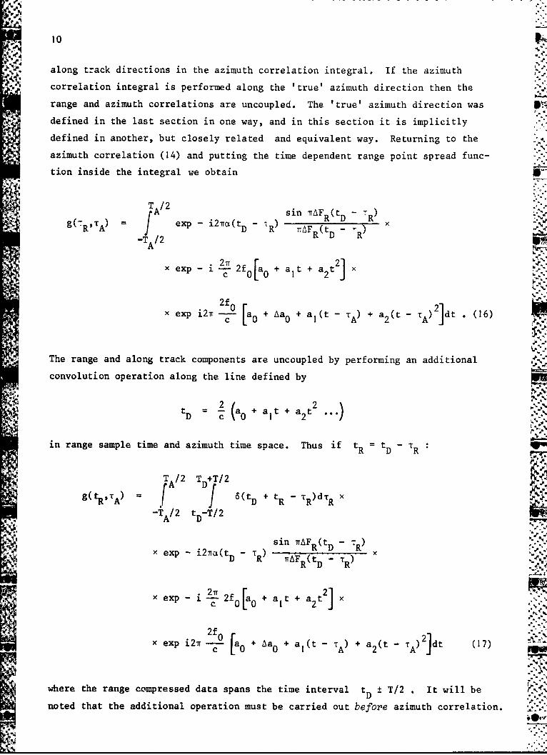
along track directions in the azimuth correlation integral. If the azimuth
correlation integral is performed along the 'true' azimuth direction then the
range and azimuth correlations are uncoupled. The 'true' azimuth direction was
defined in the last section in one way, and in this section it is implicitly
defined in another, but closely related and equivalent way. Returning to the
azimuth correlation (14) and putting the time dependent range point spread func-
tion inside the integral we obtain
A sin rAF (t - TR)](R )exp - i 2 •(tD - •R) AFRRD Rg- 9Tep i7(t I )R A D R 7TAFR(tD - R-TA/2
A
exp 2 2f1 + + %2c 2
x exp i2Tr _ [a + Aa0 + al(t - TA) + a 2 (t - dt (16)c 0 0 1) 2"
The range and along track components are uncoupled by performing an additional
convolution operation along the line defined by
21 2 )t = - a+ a t + a t
SD c 0 1 2
in range sample time and azimuth time space. Thus if tR = tD - tR
TA/2 TD T/2A Dr
I~R, 6(t t TR)dTR x*'XA f D R R-TA/2 tD-T/2
sin 7AF (t -R D Rx exp -i27a(t -T) t -ITAF R(tD R
R D R
x exp 2fr 2 + t + a x2c 0 f[a.+ 2
x exp i2r 2-_ + Aa0 + a -( ) + a2(t (1 217)c 0 a 1t A 7)
where the range compressed data spans the time interval tD± T/2 . It will be
noted that the additional operation must be carried out before azimuth correlation.
Usually the convolution is carried out by 'data selection' using more or less
approximate methods; this is explained further in section 14.
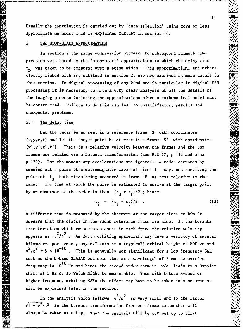
3 THE STOP-START APPROXIMATION
In section 2 the range compression process and subsequent azimutb com-
pression were based on the 'stop-start' approximation in which the delay time
tD was taken to be constant over a pulse width. This approximation, and others L 1
closely linked with it, outlined in section 2, are now examined in more detail in 1i@'
this section. In digital processing of any kind and in particular in digital SAR
processing it is necessary to have a very clear analysis of all the details cf
the imaging process including the approximations since a mathematical model must
be constructed. Failure to do this can lead to unsatisfactory results and
unexpected problems.
3.1 The delay time
Let the radar be at rest in a reference frame S with coordinates
(x,y,z,t) and let the target point be at rest in a frame S' with coordinates.
(x',y',z',t'). There is a relative velocity between the frames ard the iwo
frames are related via a Lorentz transformation (see Ref 17, p 11C and also
p 132). For the moment any accelerations are ignored. A radar operates by
sending out a pulse of electromagnetic waves at time tI say. and receiving the
pulse at t 3 both times being measured in frame S at rest relative to the
radar. The time at which the pulse is estimated to arrive at the target poirt
by an observer at the radar is then (t3 + tl)/2 ; hence
t = (t! + t 3)/2 . (18)
A different time is measured by the observer at the target since to him it
appears that the clocks in the radar reference frame are slow. In the Lorentz
transformation which connects an event in each frame the relative velocity2 2
appears as v /c . An Earth-orbiting spacecraft may have a velocity of several
kilometres per second, say 6.7 km/s at a (typical) orbital height of 800 km and2 2 -10v 2c •C 5 x 10-0 This is generally not significant for a low frequency SAR_
such as the L-band SEASAT but note that at a wavelength of 3 cm the carrier
frequency is 1010 Hz and hence the second order term in v/c leads to a Doppler
shift of 5 Hz or so which might be measurable. Thus with future X-band or
higher frequency orbiting SARs the effect may have to be taken into account as
will be explained later in the section.
2 2In the analysis which follows v /c is very small and so the factor
%4V) -- v•/,_2 in the Lorentz transformation from one frame to another will
always be taken as unity. Then the analysis will be correct up to first
12
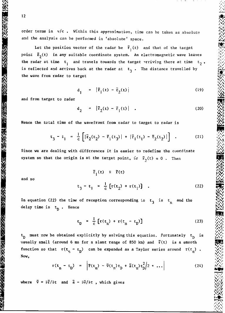
ti order terms in v/c . Within this approximation, time can be taken as absolute
and the analysis can be perfor-med in 'absolute' space.
Let the position vector of the radar be I (t) and that of the target
point i 2 (t) in any suitable coordinate system. An electromagnetic wave leaves
the radar at time tI and travels towards the target irriving there at time t 2 ,
is reflected and arrives back at the radar at t 3 . The distance travelled by
the wave from radar to target
dI = JiF(t) - r 2 (t)i (19)
and from target to radar
d t)(02 r 2 (t) - r t) 1 • (20)1
Hence the total time of the wavefront from radar to target to radar is
t 3 -tl = [' 2 '(t 2 f Fl(t 3 )I + Ii (tl) - (2 (t 2 )1] (21)
Since we are dealing with differences it is easier to redefine the coordinate
system so that the origin is at the target point, ie i,(t) 0 Then
and so
t 3 -tl - [r(t 2) + r(tl)] (22)
In equation (22) the time of reception corresponding to t3 is t and the
delay time is tD. Hence n
t [r(t) + r(tn tD)] (23)tD c n n, D
4 .
tD must now be obtained explicitly by solving this equation. Fortunately tD is
usually small (around 6 ms for a slant range of 850 kin) and F(t) is a smooth
function so that r(t - t ) can be expanded as a Taylor series around r(t .q D n
Now,
r(t t D) = - (t)tD + + (24)
where T = ai/at and a = 3-v/t which gives
Sd"N-'-
13
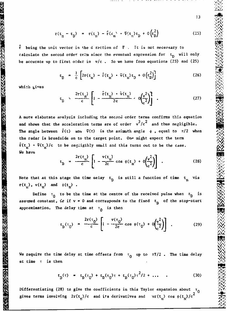
- • r(t -(c 5"'tn)t + 0 (25)r~n tD) = n) -(n n (
r being the unit vector in the d'rzction of F It is not necessary to
calculate the second order teihn since the eventual expression for tD will only •- .
be accurate up to first order in v/c . So we have from equations (23) and (25)
t [2r(t) - ^(tn) • (tn)tD + 0(tD (26)2
whiich gives -(n) (t
tD c u 0 t(27)
c€
A more elaborate ar.alysis including the second order terms confirms this equation
and shows that the acceleration terms are of order v 2 /c 2 and thus negligible.
The angle between r(t) anu V(t) is the azimuth angle * equal to n/2 when-C4
the radar is broadside on to the target point. On, might expect the termr(tn) • v(t )/c to be negligibly smill and this turns out to be the case.
n nWe have
tD == II --- cos + (tn) + 0 • (28) .'DL 2c n(t (c2J
Note that at this stage the time aelay tD is still a function of time tn via
r(tn), v(tn) and O(tin
Define T to be the time at the centre of the received pulse when tD is
assumed constant, ie if v = 0 and corresponds to the fixed tD of the stop-start
approximation. The delay time at T is then
r -
We require the time delay at time offsets from t0 up to _+T/2 . The time delay •
00
at time T is then '•
V tD(0 2/2 2)]
tD (T) = tD(O) + tD(r0)t + + ... . (30)
Differentiating (28) to give the coefficients in this Taylor expansion about 0-•2 (n22gives terms involving 2r(tn)/c and its derivatives and vr(tn) cos *(t )/
fl n n
14
and its derivatives. The maximum rate of change of • occurs for the broadside
mode and is typically a few tens of mradi/ maximum. Also, as always, v 4 c and
the leading terms only are taken in tne expansion to give
_____ 2r(T~(t ) =2Qr( 0 ) and DC = c
D OT 0 = D (T)
V and hence
(T) 2r(To) + ri0(T + r( 0 ) 2(31
3.2 Range compression with varying time delay
Let ~~t .. ._L tt (T) = TO + TIT + T I (32)
•~~ T2(3
where T I T:+ 0T (33)
and
2 2 + 2T0 T + (34)
20 22 2-2where T 2 2t + T 2 + o(3) , (35)
and from (31)2r2r(t) 2()
0O_= 0 01- -=T T __
0 C C 2 c
In addition .
T/2
f exp- i27 tD f fTr + cd~tD TR +~ 2cu(tD -RJT +T (36)
-TI/2
This is obtained by rearranging the first integral in (5), the second is ignored
for the purposes of the present analysis. qubstituting from (32) and (34) we
"Mm"- obtain
- II
15
R exp - i2N O0 0 - fITR + a(R - t 0 )
T/2
X exp - ~ + 2aT T2 + 2uTT + 2cL-iijf0-El E I E: 1 oielJI
-T1/2 .
x exp -i2ff 2aT T0 + f ] d.' . (37)0(OR) 2azJU
The first exponential under the integral contains quadratic and higher powers of
T and the second exponential contains the linear terms in T . The non-linear
powers of T result in defocissing and the linear terms simply result in a shift
in the position of the point spread function in the range direction. The quadra-.F,
tic phase term is slowly varying since the non-linear terms are small. The
linear phase term is also slowly varying in the neighbourhood of the peak of the
point spread function since T0 ! T near the peak. The non-linear term is
2£ t ! 2(3
2f T1-+ T -2 + 0(T3) . (38)
Note that T, = 2r(T 0 )/c < 2 since r v and v < c . Also 2cv >> ft T/212 I 0since a is typically of the order of 10 Hz/s . The largest non-linear
2term is then 2T I T . In section 4 it is demonstrated that a typical valueof f for a broadside looking orbital SAR at an altitude of 800 km is of
order 100 m/s. The quadratic phase change over the correlation is then of
order I mrad for a pulse width of the order of tens of microseconds. Thismagnitude of phase change is completely negligible.
The first order eftect of the stop-start approximation is a shift in the
position of the point 3pread function by f 0 1l/2a , which, for SEASAT, is about
1.5 ns or 0.45 m in slant range. This error, however, could be much greater fora radar operating at a higher frequency. Also, in a SAPR operating in a squint
mode T could easily be an order of magnitude greater. A shift in the posi-
tion of the point spread function, however, causes no real nroblems unless the
shift varies over the synthetic aperture by more than, say one half resolution
cell. Tl does vary in the azimuth direction but not by enough to causeproblems with the approximation considered here. Thus in conclusion the
stop-start approximation is valid to a high degree of precision for orbital
synthetic aperture radars.
16
4 THE RANGE POLYNOMIAL
in section 2.2, eauation (10), the range from radar to point was expanded
as a function of time:
2 3a(t) a0 + a 2t + + ... . (10)
In this section the terms in the expansion are calculated for a general elliptic
orbit, and various approximations considered.
It seems appropriate to mention here that there are at least three modes in
which a SAR may operate. These are the normal mode, the squint mode and the
spotlight mode. In the normal mode the radar looks out sideways to the tracl and
perpendicular to it. The squint mode is similar except that the radar is perma-
nently squinted either forwards or backwards to the normal mode. In the spot- V
light mode the radar squint angle is varied continuously as the radar passes a
target so that the target is constantly illuminated, and hence the syntheticaperture length is no longer limited by the footprint width. A very large aper-
ture can then, in principle, be synthesised. The squint angle is varied by vary-
ing the pitch angle and/or the yaw angle of the spacecraft depending on the angle
of incidence of the radar.
The analysis which follows is applicable (within limits) to all three
modes. Before calculating the range polynomial, however, some considerations ,ZP
concerning the choice of orbit for SAR spacecraft are nresented.
4.1 Orbits for SAR satellites
Circular or nearly circular orbits are arguably the best choice for radar
remote sensing satellites. There are several reasons for this. First, if an I
approximately constant height is maintained above the Earth's surface then the
Dappler bandwidth will remain constt.nt and this leads to a constant pulse
recurrence frequency. The prf is one of the main design parameters for a
synthetic aperture radar and if it can be kept constant this greatly simplifies
the design of the radar system. Further discussion of this point belongs to the
design of the radar rather than the processing and is not pursued here.
Secondly, if the radar data are required to be processed into images soon
after the satellite pass then nominal (and possibly inaccurate) orbital elements
will have to be used in the processing. Refined orbital parameters are not avail-
able until several days have elapsed because of the necessity of measuring the '-%
orbit at several ground stations around the Earth. The inaccuracy in the pro-
ceasing due to the use of nominal orbital elements seems to be minimised if
a circular orbit is employed, or if the orbit is frozen in some way.
It could be argued that it might be desirable to have a slightly elliptical
orbit so as to maintain (to first order) a constant height above the Earth. The
orbit apogee would then lie on the equator, the Earth being a flattened spheroid
bulging at the equator. This argument was advanced in Ref 19 in connection with
the SEASAT altimeter and such an orbit has an advantage because if the argument0of perigee is 90 (which, of course, it is if the apogee lies on the equator)
then, in principle, it is possible to choose an inclination and eccentricity AV�
such that the orbit is frozen. That is to say such that the perigee does not
precess. Normally, the perigee processes in the orbit plane by a few degrees per
day due to the Earth's oblateness. The reader is referred to Ref 19 for a fuller
account.
Another effect of the Earth's oblateness is to precess the plane of the
orbit by a few degrees per day. The rate of precession ý is given approxi-
mately by: S= -9"97(R7/2 (-e) •~
99cos a degrees/day (39)
997~) ( - e2)
see Ref 18, equation 1.1. It will be observed that this is a function of semi- 21:major axis a , eccentricity e and angle of inclination i
This effect has some importance to spacecraft designs because the rate of
precession can be chosen to be such that the solar panels which power most
satellites continuously face the Sun. This is a Sun-synchronous orbit and has
a rate of precession of approximately 3600 in 365 days. Not too much weight
should be placed on this requirement, however, because quite a large variation .on a perfect Sun-synchronous orbit is acceptable and not all spacecraft are
powered by solar cells. If one weTe designing for a synchronous orbit then once
the height of the satellite above the ground is chosen (this is a function of
radar maximum power, area of coverage, maximum data rate capacity etc) then the
inclination angle i follows for a given eccentricity. The required inclination
is greater than 900 since 2 must be positive and such orbits are known as
retrograde orbits. For example in the case of SEASAT i was slightly greater
than 1080. Of course, if the radar platform is not dependent on the Sun for its
power (as is the case for the Shuttle for example) then the orbit is not con-
strained in this manner.
The above discussion is a somewhat simplified account of the choice of
orbit for a SAR satellite. The actual details are complicated and furtherdetails of the choice of orbit for SEASAT will be found in Ref 19. .. I
:Re,_N3__%
• • -= - '-• ' .- - '1. ut'C - * . ._. 2.+ .72.o .2 -' . �.•-• i 'C -.' V- .? '-S -% ' •'.2 - i.* m%<
18
In the analysis which follows a typical orbit is assumed to be as in Fig 2.
The orbit is shown projected on to a spherical surface which is 'fixed' relative
to the background stars. The direction labelled T is the vernal equinox (the
intersection of the Earth's equator and the plane of the ecliptic) and the centre
of the surface coincides with the centre of the Earth. The point P is the point
on the Earth's surface for which the range polynomial is to be computed. The
latitude of the point is measured in geocentric coordinates and is constant, but LC
the longitude is constantly increasing due to the Earth's rotation. The point Ais the projection of the real antenna focus on to the celestial sphere. "
4.2 Latitude and longitude changes of radar and target
Let the point P in Fig 2 have a geocentric latitude and longitude measured
on the fixed surface of V) and 4. Let R be the distance of the focus of the
(real) radar antenna from the Earth's centre and r the distance of P from the
Earth's centre. Then if a is the distance between the radar antenna focus andthe point P
2 R2 r2"a =R +r -2Rr cos 0 (40)
where e is the angle AOP = AOD in Fig 2. 6 is a function of time due to the
motion of the satellite and the rotation of the Earth as indicated in Fig 2.
R is also a function of time due to the non-circular o-ic, but r is constant.
In Fig 2 D is the projection of r on to the celestial sphere upon which
the orbit has been projected, and the are AD passing through the projection of
the antenna focus A and D has on a great circle centre 0 . The meridians
passing through A and D are also great circles and triangle ADN, N being
the north pole is a spherical triangle. Let the latitude and longitude of A be
T and D in geocentric coordinates. Then from AADN we have:
cos 0 = sin T sin + co0 T cos i cos(- (41)-,)
which gives 0 in terms of the latitudes and longitudes of A(T,O) andP(ip, €)) .••
The purpose of the analysis here is to compute the coefficients a.. a
in the range polynomial2 3a = a + alt + a t + a t ...
0 I 2 3
in the neighbourhood of t = 0 . This involves differentiating (40) successively
and setting t = 0 . Hence explicitly we have:
. , , 4 - - - -•K • • _ • -' .- - • • l - • • •. . - . • a - , • • - • ~ . -* , o
19
a 0 = a at t = 0 (42)
a0 a, = 0 (R0 -r cos 60) R r -d (cos eO) (43)
0 0 0 00 0d02
2a a2 + a2 (R r cos 9 + Q o- 2 r - (CL9 0)]
- Ror -- (cos e0) (44)dt
6aa 3 + 6aa 2 ' R0 (R0 - r cos 80) + iR[2R0 - 3r d (cos e0)]
2) 3+ - 3r d (cos - R r----(cos e)kL dt 2 dt 0
...... (45)
The subscript (0) indicates that the variable is taken at t = 0 . When the
orbit is circular R and higher derivatives are zero and the equations simplify0
greatly. To proceed further it is necessary to compute derivatives of cos 0
from (41) in the region of t =0 .
Let Fig 2 show the positions of radar and point P at t = 0 , and let
the projection of the satellite move on to position B at time t , see Fig 3.
In Fig 3 C is a point on the celestial sphere which has the same geocentric
latitude as B and the same longitude as A (the position of the radar antenna
focus at t = 0). The angle BAC = v and is the 'local heading angle' of the
satellite at t = 0 . The angle AOB is the angle through which the sateliite
has moved in its orbit from A to B and AOB = Ac . Also BOC = Ar andA
AOC AT . The change in longitude, AD = BNA, AL and AD are related by
sin -T- = sin-., cos(T + AT) . (46)
The analysis is somewhat intricate and for that reason a number of the inter-
mediate steps are now set down.
The arc BC lies on a great circle and so AABC is a spherical triangle.
The angle ACB is not exactly a right angle, although provided Aa is small
(which it always is even for the 'spotlight' modes) then ACB is very nearly a
rignt angle. For example Aa is usually of the order of I mrad for normal modes.
- Angle ACB is therefore written as R/2 + c . From the sin formula for
Sspherical triangles
20
AF = sn-l~sin v0 sin Aa0Ar sin cos E (47)
To find c consider ACBN in which NCB = 7/2 - c and then
e tan'[ sin(T + AT) (I -cos AD) (48)sin A•
Spherical triangle ABC gives
AT = tan-lItan Aa - sin AP sin c (49)It0 cos A a cos AT](9
which is an implicit formula for AT .
It will be evident that computing the coefficients in the range polynomial
A directly OV means of the above formulae is not a practicable task. Fortunately,however, this is not necessary. All the angular changes AO, AO, AU, AF and f
are cf the same order of magnitude. Also Au is a first order function oftime. All terms in the range polynomial up to and including the third orderterm a are required and hence it is only necessary to expand the expressionsfor Ay, c, AT and 0a up to third order to obtain the required polynomial
coefficients exactly. Expanding (46) gives:
Ac = Ar sec T + ATAr sec T tan TO AT2Ar tan2To sec TO0 0 0 0
23AT2• Ar 233
"+ -- sec T + se T tan2 T + O(AFAT 3 , ATAr 3) (50)+ 2 0~ sc~ 04
(47) gives:3 •2 V(5At
sin o 2v AaE2 + 5 3 2 Ae4Ar An6 sin Cos0 o 0 + sin v ( + ,Aa4 t ) (51)
(48) gives:
AO ATAO AT ADE = -sin TO +-- cos T0 sin T0
2 0 2 0 4 0-..3A 3
+- -sin TO cS2os -T O(ATAý 3AOAT3) (52)2 4 0 0
and (49) gives: 21
3AO3 3 z-2 3
A = Aa cosv 0 -v Ar +- cos v0 sin v0 + O(ýA^ 2 A 2',A 2A 3 3,AF3C,AF3,
....... (53)
These equations can be manipulated to give, finally:
A2. 2 A. 3 3AT Aa cos0 --0 - sinv 0 tan 0 +- cos V0 sin v 0
_ 23 02 2
- V cos 0 sec + O(Aa 4 (54) ..2 s 0 0 0
A = Aa sin 0 sec T0 + A• 2 sin v0 cos 0 sec T0 tan Y0 0 0 0 0
Ac23 2 2--- 3sin V0 cos v0 sec 0 + Aa3 sin V Cos tan2 sec T00 0cos0 v0 tan0
AcŽ 3 2 4-3 sin V0 tan2T sec T + O(Aa4) (55)
which are the required formulae for the changes in latitude and longitude in
going from A to B in Fig 3, expressed in terms of change in satellite angle
(or 'true anomaly') Aa .
A problem arises here due to the singularity at the poles where T0 = ±n/2
and it is necessary to avoid this case in the analysis. Thus the region within
about 2' of the north and south poles is excluded. Fortunately this presents
no aifficulty because an exactly polar orbit is very unlikely to be used in
practice. The suffix (0) on the variables in equations (54) and (55) refer to
t =0 ,je n nt A in Fig 3.
Differendating (54) and (55) and setting t 0 gives:
0= 0 Cos V0 (56) ..
2 .2 2= 0 o C " , a - 0m s in v 0 ta n T 0 (5 7) ., -
+0~ Co ff ýO IO 0 ' sin2 3,VU 9 tan Y0 + 2a0 Cos V' sin v0?'•7
sin2v0 Cos V0 sec2T0 (58)
p?.?
Ti"WC WW, AIM, -. -s71 -N Z4&Oi. ýuJ
22Uý = a0 sin V 0 sec TO (59)
a c0 sin v 0 sec T0 + 2c2 sin v0 cos V0 sec T0 tan T0 (60)
O iO sin sec T0 + 6a0c0 sin v cos 0 sec T0 tanTO0 000 0 0 0 0
+ 2' 3 sin V0 cos 2 0 sec To + 6*0 sin v Cos 2V0 tan2 sec Y00 00 0 0 0 Y
-203 3 sin3v0 tan 2T sec T0 " (61)
In addition to the motion of the satellite we also have to consider the rotation
of the Earth. The latitude of a given point P remains constant but its longi-
tude increases at a constant rate • rad/s. Thus
(62)
At this point the idea of the squint angle is introduced. The squint angle is
here defined as the angle between the great circle arc AD and the great circle
perpendicular to the orbit direction at A - see Fig 2. This definition is
valid for general elliptic orbits as well as circular orbits since we consider
the projection on to a sphere. If the squint angle is zero at the centre of the
synthetic aperture at t = 0 then the radar is operating in the normal
'broadside' mode. This angle could be (and generally 4s) a function of cime due
to charges in the pitch and yaw angles of the spacecraft. The squint angle is
defined to be positive when looking forwards.
Angle NAD (Fig 2) is then 7r/2 - v0 - a0 where 00 is the squint angle at
t= 0. Note that throughout this section v is defined as positive in Figs 2 and 3.
We are now in a position to compute the coefficients in the range
polynomials.
4.3 The linear term
Differentiating (41), substituting (56) and (59) and simplifying by means
of two spherical triangle formulae for triangle ADN, viz
sin cos P0 cos(v 0 I -0) = sin T0 cos(O0 - y0) cos '0 cos(v 0 + a0)
+ sin(40 -O 0) sin( 0 + a0) cos 110 (63)0 0 0 0
23
and
sin 00 cos(v 0 + 00) = cos 0 sin(D0 - 0) (64)
givesX2. d(cos 60O)dc sin 0e sin o0 + C sin 6 cos T cos(0 + a (65)
dt - 0 0 0 0 'i0 c 0 +a0)(5
which together with (43) gives:
R Rora = (R0 - r cos 00) sin 00 sin a0
Ror0
Va0 sin6 0 cos T 0 cos(V0 + a)• (66)
Thus the linear (range walk) term neatly separates into three terms. The first
is zero for a circular orbit since R is then zero, and is thus associated withorbit eccentricity. The second term is zero when the squint angle 00 is zero
and is thus associated with the radar squint. The third term is zero when E is
zero and is thus associated with the rotation of the Earth. Thus linear range
walk is in general caused by three factors; orbit eccentricity, squint and Earth
rotation.
It is instructive to calculate aI for a typical example and the example
chosen (Fig 4) is an image from Seasat Rev.762 over the east coast of England
(the Wash and East Anglia). The coefficient a will be calculated for the
centre of the image. The Keplerian orbital elements for Seasat Rev.762 Pre given
in Table 1;
Table I
Orbital elements for Seasat Rev.762
Semi-major axis 7161.39494 km
Inclination 108.02030
Argument of perigee 148.16490"
Right ascension 89.36700
Mean anomaly 252.32420
2,
24
R and its derivatives and and higher derivatives can easily be worked out
from the orbital elements using the usual orbit equations - see for example
Ref 18, Chapter 3.
The latitude and longitudes of the satellite nadir and the centre of the
image at t = 0 (tue centre of the aperture) and values of r, RO, R0 2 R0 2 u0'
and 06 are given in Table 2.
r is the Earth radius at P and is calculated on the basis of a spheroidal6
Earth with a flattening factor of 1/298.3 and equatorial radius of 6.37816 10 M.
Table 2
Parameters of centre of Fig 4 at t 0
Latitude of nadir 51.250
Longitude of nadir -2.080
Latitude of point 52.780
Longitude of point 0.67.00 ~2. 265°
r 6.36444 x 10⁶ m _..06• R0 7.16297 x 10 m MVC-
1.37760 x 10 m/sR -1.758803 x 10 m/s20mi •'0 10-3" "
1.041312 x 10 rad/s
•0 4.005 x 10⁻⁹ rad/s2
0.7292!15 x 10 rad/s iIV 0 29.20°:
The corresponding values of the three terms in the expression for a, are:
Eccentric term: -- (R - r cos 0) = 13.147 m/sa 0 0
0
RorSquint term: - a0 sine 0 = -38.887 m/s per degree of squint
a0 for small squint angles
R rRotation term: - sin 80 cos T0 cos V = -82.385 mis .
The pitch and yaw angles of the satellite of the centre of the aperture were
about -0.0040 rad and 0.0112 rad. Because of the steep (low) incidence angle
25
the pitch angle has a greater effect on the squint than the yaw and in this0.
instance they nearly cancel out t-, give a squint angle of about -0.092 Hence
the squint term amounts to some 3.58 m/s. The squint angle Lai, easily be 0.5 or
so on occasions for SEASAT.
The linear (range walk) term is then about 65.66 m/s for this example.
One can draw some very interesting conclusions from equation (66). Notice
that it is possible to select a squint angle a0 such that aI is zero. aence
linear range walk could, in principle, be eliminated for a specific value of e0corresponding to, say, the middle of the swath by varying the squint angle of
the radar. Moreover if the orbit is circular then N
R rsine8
-l= - a0 0 [ sin au + • cos To cos(vo0 + co (67)
and a would be zero over the who 2te swath width.
In practice the centre of the Doppler spectrum (which is amplitude
modulated by the antenna beam pattern) would be measured on board the satellitf
and the satellite yaw or (better) the pitch angle would be varied via the
satellite attitude control system until the Doppler spectrum is centred on zero. muThis type of technique could have far reaching implications for the design of a 'A
SAR and processor system for real-time processing. The range walk problem is
explained further in section 12. 1 •
4.4 The quadratic term
Differentiating (41) twice, substituting from (56), (57), (59) and (60) and
simplifying by means of (41) and an additional formula for triangle ADN:
sin 0 sin(v0 + a0) = sin * cos - cos sin T0 cos(4 0 -C0) (68)
gives
d2 .2
(Cos0) -a cos 0 + 0 sin e sin a W2d0 0 0 0 0
dt1
+ 2Ect0 Sinv 0 cosio cos(P0- 0 ) - cos V0 coso sin TO sin(%O- 0
E 2 cos 0 cos 0 c°S(O (69)
The terms including • can be simplified further but only by introducing yet
another angle and so it has been left as it is. In conjunction with (43) and
(45), (69) gives: 777
26
2 2 2 RoaIa2 =2a0 0 +- r cos 60 +2a-0 - a No
A r r .2-) ý2 cos e + sin 8 sin aaC 0 0 0 0 0
S+ 2E Ojsin v0 cos q0 cos(ýo -c o) - cos V cos sin T sin( o - *o4
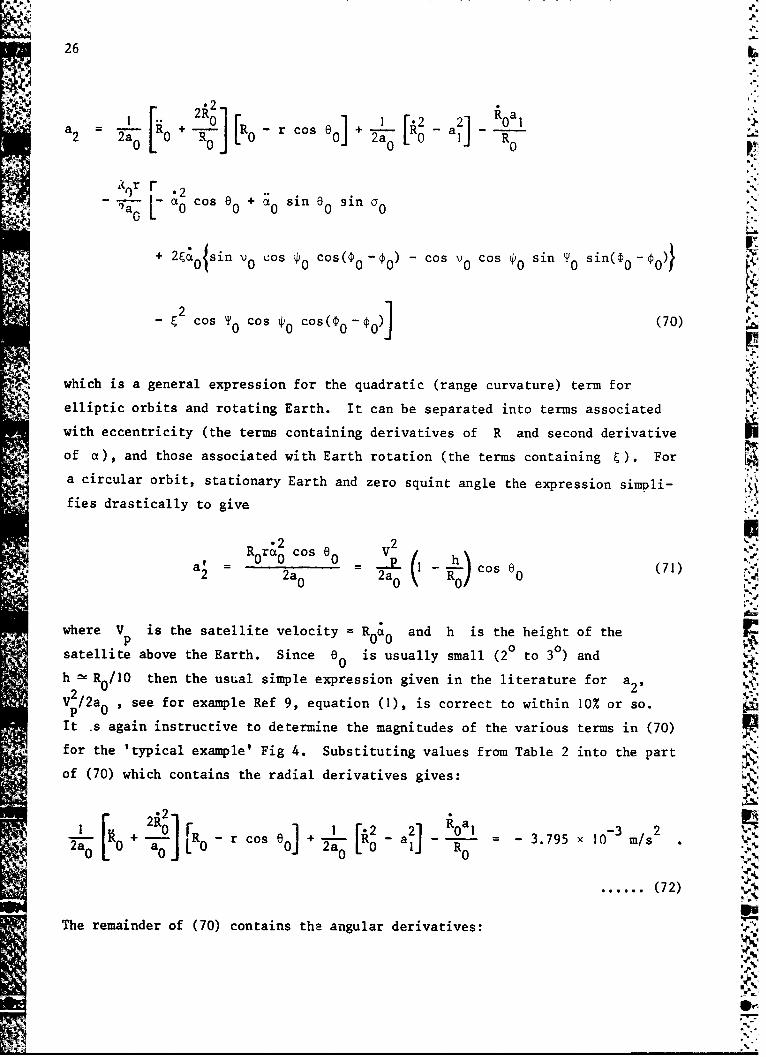
_ 2 Cos T0 cos C S0 o - (70)
• which is a general expression for the quadratic (range curvature) term for
elliptic orbits and rotating Earth. It can be separated into terms associatedwith eccentricity (the terms containing derivatives of R and second derivativeof a), and those associated with Earth rotation (the terms containing ý). For
a circular orbit, stationary Earth and zero squint angle the expression simpli-
fies drastically to give
&2 cos 02a = r cs0 h Cos 0 (71)2 - 2a0 2~a( R ~)cs 0
where V is the satellite velocity = 0 0 and h is the height of the
satellite above the Earth. Since e0 is usually small (20 to 30) and
h -N Ro/10 then the usual simple expression given in the literature for a2,
V2/2a 0 , see for example Ref 9, equation (1), is correct to within 10% or so.It s again instructive to determine the magnitudes of the various terms in (70)for the 'typical example' Fig 4. Substituting values from Table 2 into the part
of (70) which contains the radial derivatives gives:
2] rR -r o2[R0 + - r cos a+ F - a 0 - - 3.795 x 10 m/s .
A*20 L 0] 10 1i A 0a _-3
......... (72)
The remainder of (70) contains the angular derivatives:
i.--
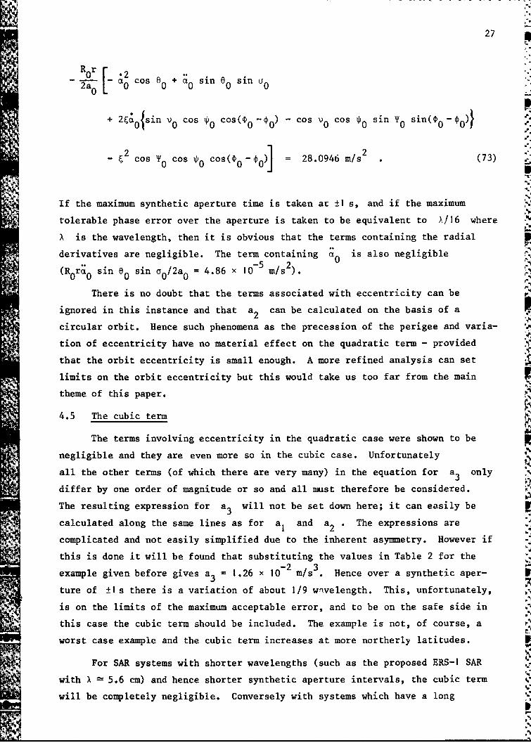
27
Rr rSCos .2 +0 sin 0 sin o0
2a - 0 cs 0 0 0 0
+ 2ýc 0 {sin V0 cos 0 cos( 0 -u 0 ) - cos V cos sin 0 sin(00
-cos T 0 cos 0 cos(G0 -4 0 )] = 28.0946 m/s 2 (73)
If the maximum synthetic aperture time is taken ar ±1 s, and if the maximum
tolerable phase error over the aperture is taken to be equivalent to X/16 where
X is the wavelength, then it is obvious that the terms containing the radial
derivatives are negligible. The term containing a0 is also negligible-5 2
(R0 rc 0 sin 0 sin a 0 /2a 0 = 4.86 x 10 m/s).
There is no doubt that the terms associated with eccentricity can be
ignored in this instance and that a2 can be calculated on the basis of a
circular orbit. Hence such phenomena as the precession of the perigee and varia-
tion of eccentricity have no material effect on the quadratic term - provided
that the orbit eccentricity is small enough. A more refined analysis can set
limits on the orbit eccentricity but this would take us too far from the main
theme of this paper.
4.5 The cubic term
The terms involving eccentricity in the quadratic case were shown to be
negligible and they are even more so in the cubic case. Unfortunately
all the other terms (of which there are very many) in the equation for a3 only
differ by one order of magnitude or so and all must therefore be considered.
The resulting expression for a3 will not be set down here; it can easily be
calculated along the same lines as for a and a 2 . The expressions are
complicated and not easily simplified due to the inherent asymmetry. However if
this is done it will be found that substituting the values in Table 2 for the
example given before gives a3 = 1.26 x 10 2 m/s. Hence over a synthetic aper-
ture of ±1 s there is a variation of about 1/9 wavelength. This, unfortunately,
is on the limits of the maximum acceptable error, and to be on the safe side in
this case the cubic term should be included. The example is not, of course, a
worst case example and the cubic term increases at more northerly latitudes.
For SAR systems with shorter wavelengths (such as the proposed ERS-1 SAR
with X - 5.6 cm) and hence shorter synthetic aperture intervals, the cubic term
will be completely negligible. Conversely with systems which have a long
UZA
28
wavelength and long synthetic aperture interval (such as the proposed spotlight
mode for the Shuttle SIR-B mission) the cubic term will be significant.
4.6 The range polynomial: conclusion
In this section it has been shown how it is possible to calculate the
terms in the range polynomial for the most general case of an elliptical orbitand rotating Earth. It has been shown that the eccentricity of the radar plat- ..
form orbit has most effect on the linear term, for small eccentricity it can be
4 neglected so far as the quadratic and cubic terms are concerned. A more refined
"analysis is possible based on this section but will not be presented here. One
implication of this is that the use of nominal orbital parameters is more likely
to have an effect on the linear range walk correction in the processing than on
focussing via the quadratic phase term. The use of 'auto-focussing' techniques
to overcome the effects of the use of nominal orbital elements is thus somewhat
questionable. All auto-focussing techniques known to the author rely in some way
on the defocussing being caused by an error on the quadratic phase over the
correlation. An error on the linear range walk can also cause defocussing due to
the selection of incorrect data in the range walk correction procedure and this
is discussed again in section 13.
5 DIGITAL PROCESSING: MATHEMATICAL PRELIMINARIES
In this section some relevant background theory is briefly presented. Most
of this theory will be found in one form or another in Ref 16. Consider a func-
tion of time f(t) ; f(t) may be complex valued. Its Fourier transform F(w)
is
F(w) ff(t) exp- iwt dt (74)
The inverse transform is
F(t) = IF(w) exp iwt dw (75)
F(w) is the spectrum of the function f(t) , and is a complex valued function.
If f(t) is purely real or imaginary then the real and imaginary parts of F(w)
have symmetry properties:
-1• if f(t) is real valued then F*(w) = F(- w) (76)
if f(t) is imaginary valued then F*(w) - F(-w) (77)
where the astccisk indicates complex conjugate.
29
5.1 The analytic signal
From equations (76) and (77) we see that a real (or imaginary) function
can therefore be completely Uatermined by only the positive (or negative)
frequencies, ie only half of the spectrum because the other half can be recon-
structed via equatiors (76) and (77). This takes us to the idea of the ai.alytic
signal.
Let f(t) be purely real with F(w) given by (74). Then F*(w) =F(-w).
Let g(t) be purely imaginary with Fourier transform G(w) . Then
G*M(w) = -G(-w) .
Let g(t) be such that for w > 0 , G(w) F(w)
Then G*(w) = F*(w) as well, for w > 0 .
Then for w < 0 we have G(-w) = -F(W)
Let z(t) = f(t) + g(t) , then its Fourier transform is
F(w) + G(w) 2F(w) W > 0
= 0 W<0
and we therefore have a single sided spectrum. Usually g(t) is written as
if(t) and then
z(t) = f(t) + if(t)
z(W) = 2F(M) ><0
=0 W <0 *.71
And so starting with a real function f(t) we can form its Fourier transform
F(w) , double it, and set its negative frequencies equal to zero. If this
function is then inverse transformed, the real part of the resulting complex
valued function z(t) is equal to the original real function f(t) . Thus onlyhalf of the spectrum of the real valued f(t) is needed to define it completely.
Now consider the function
Sa(t) exp io(t) = a(t) cos 0(t) + ia(t) sin W(t)
where a(t) and *(t) are real valued. a(t) exp iW(O) is assumed to be
analytic (and is an entire function of exponential type with singularities only
A at infinity). Then it can be proved (see Ref 20, Chapter 5) that the function
has a single sided spectrum. Hence it is possible to identify a(t) cos 0(t)
with f(t) and a(t) sin 0(t) with f(t) In actual fact f(t) and f(t)
withft ~ft
30
are mutual Hilbert transforms, but that is only of passing interest here. It
will be observed that the chirp signal, equation (3), is in this form and is an
analytic signal. Likewise (1) is the analytic signal corresponding to the real
signal (2).
Thus if we have a real valued function such as a(t) cos p(t) writing it
as a(t) exp io(t) gives the 'analytic signal' with a single sided spectrum.
It will be shown in section 6.1 that, in the case of a SAR system in which
the Doppler band extends-over both positive and negative frequencies, it is
absolutely necessary to operate on analytic signals.
5.2 The convolution and correlation theorems
If
g(t = f(T)h(t- )dT f(t - T)h(T)dT (78)
then
G(w) F(w)H(w) (79) 0"
(see Ref 16, p.21, equation (1-47)). The convolution is usually written
g(t) = f(t) ( h(t) . (80)
Hence convolution in the time domain corresponds to multiplication in the
frequency domain (and vice versa).
A similar theorem exists for the correlation function:
CO CO~
If c(t) f*(T)h(t + T)dT f*(- t)h(T)dT (81)
U then
C(w) = F*(w)H(w) .(82)
o-Y- In Ref 21, equation (406) p.768, it is shown that the complex response from a
matched filter is determined by a correlation process.
To perform matched filtering in the frequency domain therefore, one .
Fourier transforms the signal and multiplies it by the complex conjugate of thechirp replica spectrum and then performs the inverse transformation. This is the
basis of frequency domain compression in both the range and azimuth directions.
k-..-
31
5.3 The sampled discrete Fourier transform
-A The discrete Fourier transform pair analogous to the continuous transforms
are:
N-I
F(Z) f i2k (83)N L ~ k exp N
k=O
N-I
i27tk.f(k) F() exp (84)• N
This pair of transforms can be regarded as a mapping of the sequence f(k),
k - 0 ... N-I on to the sequence F(k), Z = 0 ... N-I and vice versa. There
are N samples in the 'time' domain and N in the 'frequency' domain.
The reader is reminded that it is implicit in this representation that the
original continuous time function f(t) and the corresponding spectrum F(M)
have both been periodically repeated. Usually the temporal function f(t) has
a finite length and is sampled at intervals of At , say, so that if T is the
total length T = Nht . The corresponding spectrum, however, is not finite and
the process of periodically repeating it causes the edges to be periodically-• folded into the fundamental period. This is called aliasing. The width of the
fundamental frequency period is I/At , see Ref 22, and it is therefore necessary
that there shall be no frequencies higher than f /2, where f = I/At presentS S
in the original spectrum. The reason for the additional factor of I is that we
have both the positive and negative frequencies to contend with (see Fig 5).
The frequency f /2 is commonly called the folding frequency. It will beS
observed that the sample sequence F(k) runs from 0 to N - I and therefore in the xin
first half of the sampled spectrum we have positive frequencies and in the second
half negative frequencies. The spectrum is folded about f /2 .S
There are no aliasing problems with the time sampled sequence because it is
a finite length record and is zero outside the sampled range. Each sample
in the time domain is separated by At where At = T/N and each sample in the
frequency domain is separated by Af = I/T where Af F/N and F = f thes
sampling frequency.
This discussion applies to a real valued function. When the sampled func-
tion is complex valued with a single sided spectrum then the spectrum can be
periodically repeated at double the rate of a double sided spectrum without ambi-
guity. This means that if the sampling frequency is f the spectrum can have
frequencies up to f instead of f /2 before ambiguity sets in. This can beSs s
32
Z.I =
illustrated by a simple example. Consider the real and complex signals cos 27ft
and exp i2ffft . Suppose both the signals are sampled at times n/f, n =0 ... N -I.
Then for the complex signal frequencies f and f + f are ambiguous because5
i27(f +f )n i27rf nexp= exp n (85)4'0fo f0
and for the real signal the frequencies f and f +f /2 are (just) ambiguous
because
cos[ f +] - cos . (86)
If real signals with frequencies in the range 0 to f /2 are sampled at f,
then the complex signal may be sampled at f /2 without ambiguity.5
5.4 The discrete convolution and correlation theorems ,-.r
If
N-I N-1
g(k) = •l f(m)h(k-m) = 2I 'f(k-m)h(m) (87)N,m=0 m=0.e,,
then -
G(k) = F(£)H(Z) k = 0 ... N-I. (88)
The convolutions in equation (87) and (88) are cyclic because f(m) and h(m)
m = 0 ... N -I are periodic functions. Again, then, convolution in the sampled
time space corresponds to multiplication in the sampled spectrum space.
There is a corresponding result for the correlation.
N-I N- I iif cW) f W Z (mh (k +m) = Ef*(m -k)h(m) (89)
m=O m=0.
then r..
c(9) = F*(Z)H(£) (90)
again, this correlation is cyclic.
Cyclic convolutions can produce problems (see Ref 22, p.48). For example,
in the case of the range compression process it will be demonstrated that there
"33 --
are end effects which make it necessary to process more data than is required by
the image.
5.5 Interpolation via the Fourier transform
In term. of its discrete Fourier transform (DFT) a sampled function is:
N-1f(kAt) F(kAw) exp i27rkZ 0 k N 0 (91 )
N 0p<- Z <N -I,
(see equation (84)). At is the spacing of the time samples and Aw is the
spacing of the angular frequency samples. Ai 2rAf -here Af is the frequency
sample spacing
A t =.L - 2r(92)t=NA-- =NAw "
Suppose that the length of the inverse DFT is doubled and define a new set of
spectrum samples F'(ZAw) such that
F'(kAw) = F(ZAw) for 0 < <N-1 (= 0 for N < < 2N-1.
Then the new inverse DFT is:
2N-1 N-1i2k i2Tr£kF'(Ww) exp 2N =exp
2N 2N
S= F(kAw) exp N(94)X=0
Comparing this with equation (91) gives:
2N-I
FI O.Aw) e i2Tirk f kAt (95)E •2 e N 2-
Since the number of samples in the inverse DFT was do-,bled, the numbers of
samples of the time function f(t) was also doubled and there are therefore
34
2N samples at intervals of At/2 . That is to say the time function has been
interpolated. All the original samples exist and in addition there are new
(interpolated) samples midway between the original samples.4N This process can evidently be continued and if the inverse DFT is per-
n *nformed with a length 2 times the forward DFT this gives 2n- I in erpolation
points.
Some further comments will be made on the process in section 6.3. There is
another interpolation technique using the DFT which is not limited to dividingthe sample interval by some power of 2. Returning to equation (91) it is evident
thatN-1!v••
I ~ i27rkk x i21TaZ,f(kAf + xat) = F(£Aw) exp N N (96)N ep N
It is therefore possible to produce new samples at any chosen point within the
original intervals (a < 1) simply by weighting the spectrum samples by a phase
shift exp(i27ac/N) before inverse Fourier transforming. '0
Both of the above techniques have successfully been used on S.AR processing
at RAE.
6 SPECTRA
6.1 The range spectrum
The signal transmitted by a SAR is usually a frequency modulated 'chirp'
with a large time-bandwidth product. The spectrum of such a chirp is calculated
in Ref 16 (example 8-5, p.270). It is a Fresnel integral. If the chirp is"I centred on f (the radar 'carrier' or centre frequency) and has a nominal0
width of AF (= the chirp rate in Hz/s x the pulse width) then the spectrum is
as sketched in Fig 6. This is the spectrum of the real valued signal (2) asobtained by the radar receiver from a point scatterer. The actual signal as it
exists in space is complex valued and has a single sided spectrum for
reasons which will not be pursued here.
Fig 2 shows the modulus of the complex valued spectrum as do all the
subsequent figures.
Each point on the ground reflects a replica of the transmitted chirp and
the received signal at any instant is the linear sum of chirps reflected from
points illuminated by the footprint and within a distance corresponding to half
a pulse width. The bandwidth of the received signal is therefore the same as
35
N• that of a single chirp, although, of course, the detail of the spectrum is
•'•- -greatly different and is noise-like being composed of chirps with random phases
and displaced in time.
The actual received spectrum is sketched in Fig 7.
The receiver coherently mixes the sigaal down to the offset video frequency. •- -*
This offset is chosen to be slightly ,teater than AF/2 to avoid aliasing the W7
spectrum and is one quarter of t1e subsequent digitising frequency for a real
valued signal. The resulting spcct- am is shcjw. in Fig 8.
The signal is still r-al valued at this -oint. At this stage the signal
could be operated on by ;o qcu-dratuie filter to give the analytic signal in which
case the negative half of the spectrum disappears and then f| could be mixed
down to zero to give a spectrum symmetric about zero. The resulting signal
would be complex valued. For the moment, however a real valued signal will still
be used.
- Tbe signal is next digitibed at a sampling frequency f (typically exactlyS
four times the offset video f1 ) T The process of sampling the signal causes the
spectrum to be peiiodically •epeated at a frequency of f - see Fig 9. Just the •
envelope of the spectrum is shown in Fig 9, the positive and negative frequencies
are indicated by '+' and '-'. -"
When range compression is performed in the frequency domain (as it nearly
always is) using a discrete Fourier transform (the 'fast' Fou•ier transform
version) then the spectrum is also sampled. If N samples are used in the
Fourier transform the spectrum is sampled with a frequency incz•z--nt of f IN5' A
from sample to sample, see Fig 10. In the case of the fast Fcurifr transform F%:ý
there will be 2 n samples, typically 4096, 8192 or 16384 for a spacecraft SAR.
Notice that the positive frequencies are contained in samples I to N/2 and the
-0 negative frequencies in samples N/2 + I to N . The chirp spectrum is similar
and thus the product of the chirp and signal spectra is similar.
At this stage the negative frequencies are eliminated by setting samples
N/2 + I to N equal to zero, and on inverse transforming, the compressed
analytic signal is produced. -"
6.2 The azimuth spectrum 6-6
Previously the spectrum of just one pulse was considered. Now, tlhe
spectrum of a large number of pulses is discussed. Fig 8 gives the specttum of
just one received pulse at the offset video frequency. The radar periodicallyrepeats pulses at a pulse recurrence frequency of v Hz, say. The effect of thisis to turn the spectrum in Fig 8 into a line spectrum. The distance between the
36
lines is v Hz • The resulting spectrum of a large number of received pulses is
shown in Fig 11. This should not be confused with the line spectrum already
considered in Fig 10. That spectrum arose in the range compression process, a j ..
process independent of the azimuth direction.
The spectrum shown in Fig 11 would be obtained if the radar platform were
stationary. The platform moves, of course, and each of the lines in the spectrum
therefore moies due to the Doppler effect.
Suppose that range compression is performed using real data. The result
is given in equation (6'. The Doppler 'phase' term is a cosine function. If
range compression is performed with an analytic signal the result is given in
equation (7) and the phase term is an exponential. This is a crucial difference.
Consider just one line in the spectrum of Fig II. If the real 'phase' term is
used then a Doppler shift splits the line into two lines because the cosine term
implicitly includes both positive and negative frequencies - see Fig 12. In
other words positive and negative frequencies are indistinguishable, ie aliassed. '-
For the analytic signal with a single sided spectrum a Doppler shift just shifts 4.
each line as shown in Fig 13. There is only one line and posicive and negative
frequencies are kept separate.
In actual fact one has a continuum of Doppler frequencies both positive
and negative for a broadside looking radar. Each line is then broadened into a
continuum - see Fig 14.
- -~ Note that the radar is designed in such a way that the pulse recurrence
W frequency is high enough to sample the Doppler band defined by the antenna beam-
width and this is done on the basis of an analytic signal.
If the radar is a pure squint mode radar with only positive or negative
frequencies then the aliassing problem would not exist. One could then either L
choose a high enough pulse recurrence frequency or a very carefully chosen prf
so that the Doppler band is aliassed into a wholly positive or negative band.
This would undoubtedly lead to problems both with the design of the radar and
the spacecraft attitude control.
In any event for a broadside looking ridar the Analytic signal is always
an absolute necessity and is probably also necessary for practical reasons for
a pure squint mode radar.
6.3 Interpolation
In section 5.5 an interpolation technique was described in which the dataU to be interpolated are Fourier transformed via a DFT and then inverse transformed
via a DFT with a larger number of samples. In using this technique one has to be
37
careful to treat the spectrum correctly. This will now be described, with
reference to interpolating range compressed data.
Consider the sampled range spectrum shown in Fig 8. It corresponds to a
Fourier transformed pulse. Both pulse and spectrum are sampled and periodically
repeated. The period of the spectrum is f , the sampling frequency. Suppose5
that there are N samples. N/2 cover the negative frequencies and N/2 the
positive frequencies, see Fig 9. Increasing the number of samples in the inverse
transform is equivalent to sampling at a higher rate and the spectrum is period-
ically repeated at a longer period mf , say, where m is an integer equal to ,-A
some power of 2. The resulting spectrum is shown in Fig 15. In order to achieve
this the negative frequencies which occupy samples N/2 + I to N in the
original spectrum must be moved up to samples mN - N/2 + I and mN in the new
spectrum before inverse transforming as shown in Fig 15. Everything will then
be correct and the correct interpolated samples will be produced.
7 SIDELOBE REDUCTION - APERTURE AND SPECTRUM WEIGHTING
Equation (15) gives the point spread function in both range and azimuth for
the ideal matched filtering process. The modulus of the point spread function in
both directions is of the form Isin x/xJ . This function is plotted in Fig 16.
It will be observed that together with the main lobe there are sidelobes. These
sidelobes are usually considered to be objectionable, although the author has
processed images both with sidelobe reduction and without and can rarely tell the
difference. The sidelobes are noticeable in the case of very bright point-like
scatterers.
It is possible to reduce the level of these sidelobes but only at the
expense of broadening the main lobe, ie reducing the resolution.
If the correlation process (matched filtering) is performed in the time
ýomain then an integral of the form:
to+T/2
Jg(T)J F exp i2r-AF -L dt (97)Tt 0 _T/2
is obtained. If the correlation process is performed in the frequency domain an
integral of a similar form is obtained (this is the inverse Fourier transform of
the product of the spectra of the signal and chirp replica or phase history
replica).
SO1f-
38
f+F12exp i2rtAF -df (98)
f 0 -F/2
where the time centre of the aperture is to , the frequency centre is f 0 o
the time width is T , and the frequency width is F (this is equal to AF but
formula (98) has been written as it has in order to exhibit symmetry with (97).
Sidelobe reduction is obtained by weighting the integrals in (97) and (42).
A discussion will be found in Ref 21, section 3.4.2 p. 7 8 0 . Such weightiig func-
tions are usually expressed as a Fourier series with a period of either T or
F . There are very many of them. The ideal function (ideal in the sense that
one obtains minimum mainlobe broadening for a given sidelobe reduction) is the
Dolph-Chebycheff function - see Ref 21, section 3.4.2.2 p. 78 2 . In Ref 16
Papoulis lists a number of different functions (section 7.3, p.234).
By far the most popular weighting function is a 'raised cosine'. This will
be recognised as simply the first two terms in a truncated Fourier series. This
it -1so known as a Taylor weighting function - see Ref 21.
The time weighting function is:S-t 0
w(t) = 1+2 cos t T/2 t -T/2 < t < t0 +T/2 (99)
and the frequency weighting version is:
[T(f -f 0)]w(f) = I + 20 cosL AF/2 J -AF/2 < f < f 0 +AF/2 (100)
Sis a parameter 0 < a < which specifies the sidelobe levels. The resulting
point spread function is:
Fsin TrATFT r + 2a (101)
(TAF)) 2 - 1
and the phase part of the psf is unaltered.
The signal energy is increased by a factor of I + 282 in both frequency
and time domain correlations since
T/2Iw2 02w(t)dt =I + 2~ (102) S
-TI2
39
The first zero in the point spread function is located at /1/(I -2ý)/AF the
position of the other zeros are unchanged. The relationship between • and the
sidelobe levels must be obtained numerically. NO
An alternative to the Taylor weighting function is the Chebyshev weightingfunction, as pointed out above. This weighting function is best designed by .
means of the Remez exchange algorithm - see Ref 23, p.1 3 6 . The sidelobe levelsE07
are specified and the number of weights, and then the design algorithm gives the
weights. Sidelobe weighting using this type of weighting function has been Vsed
in Ref 9.
8 RANGE COMPRESSION
The various aspects of the range compression process have been discussed in
previous sections and now in this section they are collected together.
Range compression is usually performed in the frequency domain using the
correlation theorem in section 5.2 and the discrete Fourier transform in section
5.3. The fast Fourier transform (FFT) version of the disct~to Fourier transform
(DFT) is invariably employed - see Ref 22 for a description of the FFT. The FFT
is just an efficient way of computing a DFT. In order to use it the number of
samples must be some power of 2, ie N 2 n
The question of how many pulses and which pulses to compress is considereid
in the sections on prefiltering and azimuth compression. .,",'.,
It is interesting to examine the difference between correlation via the
time domain and via the FFT. The number of multiplications and additions for the ,•. -
FFT is given in Ref 22. If there are N complex samples in the signal and n
complex non-zero samples in the replica then correlation via the FFT requires
approximately N(I +log2 N) multiplications and 2N log2 N additions, and straight
correlation requires nN multiplications and nN additions. N > n because the -V
replica is much shorter than the signal for obvious reasons.
repliAs an example consider SEASAT. If one chose 8192 real range samples out of
a total of 13680, ie 4096 complex samples for the analytic signal, and 1536 real
value samples (768 complex) for the chirp replica then the FFT correlation
requires 53248 multiplications and 98304 additions and subtractions. Straight
correlation requires over 3 million multiplications and 3 million additions.
V Correlation via the FFT is therefore much faster.
All pulses are correlated against the same chirp replica. This chirp
replica is known from the system specifications. Sometimes it has to be
adjusted slightly in order to achieve the best possible range focussing. ',-
F:
S~40
,. ..
The chirp replica, then, is sampled at the same rate as the data. The chirp
record length is packed out with zeros to make it the same length as each pulse
record length ( 2 , as pointed out above). The packed record is then Fourier
transformed and conjugated, the resulting spectrum is then weighted by the side-
lobe weighting function given in section 7, suitably sampled. Naturally the
spectral width of the weighting function AF is the same as that of the chirp
spectrum. The weighted chirp spectrum is then permanently stored and used to
correlate all the pulses. Each pulse signal is taken out of bulk storage and
either parked with zeros to 2 n or t "ncated (this is more usual). Each
pulse is then Fourier transformed, multiplied by the weighted chirp spectrum,
and inverse Fourier transformed. This process is continued until all the pulses
required to process the image have been compressed.
The reason for the truncation (or packing) of the pulse samples is that the
total number of samples in each pulse is never, in practice, an exact power of 2.
For example in the case of SEASAT N = 13680. There are then two choices and,
usually, considerations of total storage for the range compressed pulses dictate
that each pulse be truncated to 8192 or less.
It will be recalled that the FFT correlatior is a cyclic correlation -
see section 5.4, and this will now be examined. The signal samples can
(schematically) be placed at equiangular points around a circle, and the chirp
replica also, see Fig 17. The cyclic convolution then implicitly involves
multiplying each signal sample with the corresponding replica sample, adding,
and then rotating the replica relative to the signal by one sample and repeating
the process N times. The FFT correlation does not do this explicitly, of
course, but is entirely equivalent.
If the signal has been truncated it is easily seen that some signal has been
lost for a time of T/2 at each truncation point, where T is the chirp width.
It will be recalled, that due to the finite chirp width, the signal reflected fromS each point scatter does not extend over the whole signal but only over an interv~l
of T . Hence if both the beginning aad end of each pulse have been truncated the
signals will not be properly correlated over cn interval of ±T/2 around the
'join' in the cyclic correlation. The top and bottom of thi resulting image willN then be spoilt over a distance corresponding to half a pulse width. It is there-
fore necessary to bear this in mind when selecting range samples to cover a par-
A�ticular image and a contingency of T/2 is required at the beginning and end of
each pulse. An additional contingency is required to cover range migration and
this is explained further in section 13.
41
It remains to be shown how the offset video frequency fl is removed,
see equation (7) and subsequent remarks. This can be done immediately before
inverse Fourier transforming each product spectrum, ie after each signal spectrum
has been multiplied by the replica spectrum. As pointed out in section 2. 1 the
offset video is often arranged to be one quarter of the real sampling frequency.
This is one half of the complex sampling frequency (the product spectrum at this
stage is that of the analytic signal). If the offset video f is exactly half
of the maximum frequency in the spectrum then to translate it to zero the spectrum
is simply moved by one half period. The procedure, then, is to rotate the
product spectrum in either direction by N/2 before inverse Fourier transforming.
The offset video can also be removed in the time domain, after inverse
transforming, by reversing the sign of alternate samples. Equation (7) gives the W.,
phase progression due to the offset video as exp i27flt . If f is theIn .0,
sampling frequency of the real data, f s/2 is the sampling frequency of the
complex analytic signal and the time increment from sample to sample is 2/fs
Hence t = n(2/f ) and f = f /4 and then exp i 2 7fftn = exp inn = (-I)nn s 1 n
These procedures can obviously be generalised to cope with the situation in which _,.':
the offset video frequency is not exactly one quarter of the sampling frequency.
9 LOOK FILTERING
In the processing of an image the Doppler spectrum is usually divided
into a number of equal parts and a separate image is processed from each part.
Thus each image is processed from a sub-aperture. The radar is designed to have
an adequate Doppler bandwidth to permit this and if an image is processed using
the whole Doppler bandwidth the resulting azimuth resolution is many times finer
than the range resolution. Each image processed from a sub-aperture is detected
(ie the modulus is formed, or an intensity image formed) and then the images are
added incoherently. The objective is to produce speckle smoothing, that is, an
improvement in the radiometric resolution at the expense of spatial resolution.
An explanation of how speckle arises will be found in Ref 24.
Eacn sub-aperture is generated by means of a digital band pass filter - the -\-j
'look filter' - centred on to a different part of the Doppler spectrum. The
filtering can be performed before the azimuth correlation process in which case
it is known as prefiltering or alternatively, during the azimuth correlation
process. In principle it could also be carried out afterwards but this is never
done for reasons that will become clear.
Prefiltering has computational advantages. Suppose that the aperture '
.Doppler spectrum) Is divided into M sub-apertures each of width AF /M whereA
AF Ais the total Doppler spec LLum. It is then evident that since we have an PtA.
42
analytic signal it is possible to subsample the Doppler phase and reduce the
number of pulses which it is necessary to process. Thus for M sub-apertures
it is oniy necessary to process every Mth pulse.
9.1 Design of the prefilter
The first requirement of the prefilter is that it should not introduce
spurious phase shifts into the data, since this will have serious consequences
for the azimuth correlation process. A linear phase response (as a function of Lfrequency) might just be tolerable since this would just shift the image in the
azimuth direction. It is, however, possible to design a digital filter which
introduces no phase shift at all. This is one of the advantages of operating
with digital data; a zero phase shift analogue filter is impossible!
There are basically two types of digital filter, the finite impulse response xi
(FIR) and the infinite impulse response (1IR) filters. Only the first type can
be designed to have zero or linear phase shifts. It is possible to utilise a
filter which has a non zero phase shift by passing the output of the filter back
through the filter in reverse time sequence. This removes the phase shifts and
is called two pass operation. However, this filter requires all the output
pulses to be realised, not just every Mth pulse. Tn addition this type of filter
causes difficulty with the data management. There are similar problems with the
recursive filter. An additional problem is that it is not straightforward to
change the filter characteristics in 'mid image'.
By far the most straightforward design is the phase-shift free non recursive
filter and this is the type which has been used in the RAE processor.
FIR filters are explained in detail in Ref 23.
Consider a sequence h(n) - < (N 2 1 N odd. These may be
regarded as the filter weights. The discrete Fourier transform of this sequence
is
(N-I) 02
H(exp w) = h(n) exp- iwn (103)
n=-( )/2
and this defines a finite Fourier series period 2n and gives the frequencyresponse of a non recursive filter. If there is no phase shift then obviouslyH(exp iw) is real, and this is true if h(n) = h(-n) and then
(N-I) i2
H(exp iw) h(O) + 2 " h(n) cos wn (104)
MnR.
This argument also works for N even in which case 43
N/2
H(exp iw) 2>'h(n) cos wn (105)
n=I
It is therefore possible to design a filter in which there is no phase shift.
It will not be demonstrated here, but the case N even leads to problems because
the output time samples occur midway between the input samples. Hence filters
used for prefiltering have an odd number of coefficients and have symmetric
coefficients.
One way to design the filter is the 'window method'. First of all we
decide on the shape of the required response. The ideal (from one point of
view) is the rectangular function shown in Fig 18. This is not realistic,
however, because it requires an infinit aumber of Fourier coefficients and
hence an infinite sequence of input samples. The resulting Fourier series is
truncated therefore and then the coefficients are:
h(O) = (106)
nw/v
h(n) = sin 2-- n #0 (107)
where v pulse recurrence frequency, w = cutoff frequency (rad/s), and-(N -1) /2 •<n •< (N -1) /2.
Due to the Gibb's phenomenon there are ripples in the pass band and in the
stop band and the amplitude of these ripples is not affected by the order of the
filter N . These ripples may be smoothed by a weighting function and this
function works in exactly the same way as the sidelobe weighting function in
section 7. Typically, the Hanning weighting function is used
,n
w(n) = I + cos-!- (108)k
N + Iwhere k = 2 (109) ,'
and thenW
h(O) c ( 10
nw /V[+ cosjis _Ln ch(n) = sin--- (IlI)
k~I 2 T-
~44
Substituting in equation (104) then gives the filter response function: W
N-1I, .- ,S-c (I + cos nfr/N) sin nw /v cos nw/v
H(exp iw) = + . (112)
n=l I
The band centre can be shifted by weighting by an exponential weighting function:
i21frf nh'(n) h(n) exp (113)
The sub-sampling and weighting procedure is then described by:
(N+)/12
S'(m) = h(n)S(n + Mm) (114)
n=-(N-1)/2
M is the data reduction factor and S(n), n = I ... are complex range compressed
pulses. S'(m) are the prefiltered pulses. It is important that the prefilter
be as simple as possible since too great a complexity will reduce the computa-
tional advantages gained from data reduction. So minimum N consistent with J.•
sufficiently low ambiguities is chosen. The ambiguities are caused by non-zero
response in the stop band, ie aliassing, and they also depend on the data reduc-
tion factor. Response curves for this type of filter are given in Ref 11.j
Prefiltering has advantages for both frequency domain azimuth processing
and for time domain processing. The reduction of the data rate means that corner -.7,
* turning (see section 10) can be done on smaller arrays with consequent time
saving and the forward FFT processes a smaller amount of data. The savings for
time domain processing can be considerable. The number of multiplications intime domain processing is proportional to the square of the number of pulses,
reducing the data rate by 4 (for 4 look processing) reduces the number of multi-
plications by a factor of 16. Likewise the number of multiplications in perform-
ing the FFT is proportional to N log2N and is thus reduced by a factor of 8.
9.2 Frequency domain look filtering
Look filtering can be performed in the frequency domain, and this approach
is commonly followed in processors which perform azimuth correlation in the
frequency domain, see Ref 9 section 3.3. An azimuth line is assembled for
azimuth compression (see section 11 for an explanation of this process) and @1'.O
45Fourier transformed to give the corresponding spectrum. This spectrum ther.
covers the whole Doppler band. If M looks are required then this spectrum
could be simply split up into M non zero bands. However, the opoortunity can
be taken here to introduce sidelobe weighting at the same time. Simply splitting
up the spectrum would result in an image azimuth point spread function of
'sin x/x' form assuming there is no weighting applied to either the Doppler
spectrum or replica (see later sections). This subject is further explored in
the sections on azimuth compression.
10 CORNER TURNING
After range compression each pulse is stored on a direct access bulk
storage peripheral - invariably a disc file unit. Such disc file units store the
data serially line by line. Moreover the data are usually transferred to and from
the disc file in the form of blocks of typically 1024 16-bit words. These blocks
are stored at random on the disc wherever there happens to be space. It is evi-
dent that if a matrix is stored row by row and it is reqt.ired to aecess the
-• columns of the matrix then very many blocks will have to be retrieved from the
disc because each block will contain few column elements. Indeed if the length V-1
of each row in the matrix exceeds 1024 words (which is invariably the case with
SAR data) then one block will have to be transferred for each column element. _
In order to set up the data for azimuth compression it is necessary to take
samples from each pulse, ie to read along the stored 'columns'. Unless the data
are organised correctly this process becomes hopelessly inefficient, and con-
sequently time consuming. Wa
There are a number of techniques available for reorganising the data. One
of the simplest and more efficient methods is to transpose the data so that the
stored blocks contain the data in serial column form rather than serial row form.
This process is known as 'corner turning'. This transpose operation can itsell
be carried out in a number of ways. The technique described by Eklundh25 is
optimum in terms of the number of operations carried out, but its implementation
depends on the individual computer system and it has to be modified to handle non
square matrices.
"Corner turning is not strictly necessary, and indeed it is not used for
example in the RAE processor. It is used, however, in both the Jet Propulsion7Laboratory processor in the USA and the processor designed by Macdonald,
9Dettwiler and Associates in Canada . One alternative strategem is to write special
low level routines to transfer data on and off disc in large blocks, taking advan-
tage of the structure of the disc file unit to incorporate some parallel reading and •
writing to and from the columns formed by the tracks on the stack of plattens
N-N\
jp
46
which make up a disc file unit. The size of the blocks is limited in various ways
by the host computer. When data are read off the disc for azimuth compression,
then this is done in large (64 kbyte) blocks. The shape of each block, ie therow and column lengtl-s is chosen to maximise the number of new image points which rOli•
can be processed (in azimuth) using the data taking into account the range migra-
tion. Then all the image points which can be processed using this data, and
which have not previously been processed, are processed.
The organisation of the azimuth data for both frequency and time domain W_7
processors will be discussed further when the effects of range migration are
examined.
It should also be pointed out here that if a large enough random access
memory is available to store all the range compressed data to process a given
image then corner turning is not necessary. At the time of writing such very/3.,
large memories are just possible but they are expensive. Matters will, however,
change and in a few years' time it is probable that corner turning will become a
thing of the past. SAR processor designers have this point actively in mind and
future designs will undoubtedly feature large fast random access memories.-,- -'..•
11 AZIMUTH COMPRESSION WITH NO RANGE MIGRATION
11 . 1 Frequency domain versus time domain
As pointed out in section 2.2 azimuth correlation is essentially the same
process as range correlation. It may be performed either in the time domain or
in the frequency domain via the FFT. For a small number of samples correlation
via the time domain is faster than via the FFT due to the inherent speed
advantage of the FFT method being outweighed by the greater time penalty of
memory read/write operations. For larger N , however, the FFT method is much Q
faster, the cross over point depends on the processor, and for the Floating Point
Systems API20B for example, lies between 64 and 128 points. Satellite SAR azi-
muth processing is performed on data sets of several thousand samples. Hence,
when there is no range migration there are clear advantages for processing in the
frequency domain. The situation when there is range migration is discussed in
section 14.
11.2 Data selection and packing
Let the velocity of the radar platform be V and the prf v . Then theP %
distance between pulses on the ground is V /v metres. If the image has a lengthp
L in the azimuth direction then Lv/L pulses are required, ignoring, for thep
moment, 'end' effects due to: (a) extra pulses at each end of the record being
required to ensure that all the pulses which cover the image points at the ends .• '.
of the azimuth line are included, and (b) to cover end effects in the correlation.
~~~~V" -' 2 -77 .7%b. ~
47
The required resolution determines th! Doppler bandwidth AF - see equation (15),AFA is easily shown to be approximately (ie to first order) 2V 2TA/a0 where
T is the synthetic aperture time interval, a is the range to a chosen pointA0
at t = 0 , ie broadside on in this case. Hence for a constant AF (ie constant
resolution) T must increase across track with a 0 . This happens naturallyA0
because the projected width of the antenna footprint increases linearly with a0
across track, see Fig 19. It does mean, however, that in order to maintain
constant azimuth resolution across track the number of samples in the azimuth .
data (ie the number of probes) must be increased as each azimuth line is pro-
cessed. In addition the number of samples in the azimuth chirp replica
exp - i2rf t' (equation (13)) must also be increased. Also the contingencies0OD
mentioned above to cover the ends of the azimuth line, are also range dependent.
Consider, for the moment, the processing of the whole azimuth spectrum to
obtain a maximum resolution one look image. If the azimuth length of the
required image is L , the prf v and the radar velocity V then evidently
the number of pulses required is Lv/V . The number of samples in the Dopplerp
replica against which the signal is correlated is given by the aperture timeTA = AF Xa0/2Vp and the prf, v . That is the number of samples = vT A
The contingencies should ideally be added to the longer of the two records,
ie if the number of pulses n > n , the number of replica samples then thep rcontingency (= nr/2 for each of the two contingencies (1) and (2) given above,
ie n ), should be added to each end of the n record.r p
In order to perform the correlation via an FFT the number of samples
should be 2 and one has the option of either packing the record lengthnwith zeros or choosing a record length (including contingency) equal to 2 .
In fact both the signal record (azimuth line) and azimuth replica expand as
each azimuth line is processed moving across track in order to maintain
resolution.
If one is prepared to accept a variation in azimuth resolution across
track then constant length records are acceptable. In this case it is only
necessary to pack one record (probably the replica) whereas in the former case
it is necessary to pack both. However variable length records do not constitute
a major problem.
11.3 The replica
The replica is exp - i27rf t' with t' given by equation (13) except that0OD D
in this section it is assumed that a, = 0 , ie there is no range walk. The
replica is then the same for all points along a given azinuth line at constant
range sample number, the only difference being a shift in the time axis. This
EiIp -
48S 48
translates into a phase shift in the spectrum and therefire all points con-
tribute the same spectrum (scaled by the scattering cross sections) with differ-
ent phase shifts. Thus all points may be correlated by the same replica
spectrum and, on inverse transforming, these phase shifts translate back into
time shifts and each focussed point is returned to its correct sequence in
the image line.
The range history is computed for each azimuth line, but is constant for Ce
that line once computed. It is emphasised that in this section it is assumed
that there is no range migration effect (which is valid for most aircraft SARs
for instance). The replica is computed at time increments equal to the time
between each pulse and the number of samples corresponds to the number of pulses
in the aperture, or sub aperture.
11.4 The correlation process
This is identical to the range compression process described in section 8.
The Doppler signal (the azimuth line) is Fourier transformed via an FFT. The
range history is computed and Fourier transformed, complex conjugated and the two
spectra are multiplied together, multiplied by the sidelobe reduction weights ,"%
(section 7), inverse transformed, and the image line stored. The end image
points in the record corresponding to half the replica length are rejected since
they are not properly correlated.
So far 'one look' processing with the entire Doppler spectrum has been
assumed. In practice multilook images are usually required and each separate 1.1
look is produced by processing a sub-aperture. This can be done by processing ,
prefiltered data (see section 9) or by selecting a sub-aperture during the
correlation process (as is done in Ref 9 for instance).
When processing prefiltered data the processing proceeds exactly as before
except that the effective prf is now reduced by the data reduction factor (which
equals the number of looks). Thus to process a given number of image points
requires fewer pulses. Naturally, each look is processed from a different set
of prefiltered data so that the total number of pulses processed remains the
same. However overall processing time is shorter because it depends upon the
number of pulses in a non-linear way. The effective prf is reduced by the data
reduction factor M and there are fewer pulses in the aperture, but since the
(sub) aperture is now reduced in width also by a factor M the total number of
pulses in the aperture is reduced by M2 (16 for a 4 look system). Hence if
there are approximately 4000 pulses in the full aperture (for SEASAT) there are
only 250 effective pulses in one quarter aperture (approximately). For an eight :0'
look system there would only be 63 or so and time domain correlation would begin
to become a possibility!
Hence in the construction of the replica the range history is computed at
intervals of At/M where At = I/v and only for those samples within an interval
of T/M where T = full aperture width. Note that each sub-replica is computed
using exactly the same parameters, the sub-replicas only differ in the range of V
time over which they are computed. This automatically ensures that the azimuth
image lines computed from each sub-aperture are correctly registered. The process-
ing then proceeds as before. The sub-replica is packed with zeros to make ic1_
the same length as the azimuth line (in terms of the numbers of samples), Fourier
transformed, multiplied by the sidelobe reduction weights, multiplied by the com-
plex conjugate of the Fourier transform of the azimuth line and then inverse
transformed. This is repeated for the other sub-apertures. The imperfectly
correlated image points A- the beginning and end of the image lines are rejected.
The modulus of each of •ne complex valued azimuth lines is taken and they are
added incoherently to produce a smoothed image line.
An alternative strategy to prefiltering the data is to generate the looks
during the correlation process. Again, the processing proceeds much as in the
full aperture case. The pulses covering the required azimuth line (all of them) mUnare selected and a contingency added at each end. They are packed to 2n
and Fourier transformed. The spectrum is then split up into a number of
separate contiguous sections. These are the looks. The replicas are constructed
exactly as in the case of the prefiltered data and the correlation is then
performed in the same way. This technique is used in Ref 9: it will be noted
that the sidelobe reduction filter used in Ref 9 was of a different kind from that
suggested here, having a linear phase equal ripple Chebyshev response, see
section 9.2.
11.6 Azimuth correlation point by point
This technique is very slow in comparison with the block processing
inherent in the FFT correlation. It is not limited to a fixed pixel spacing of
V /AF •p A
The pulses covering the target point are selected and the azimuth phase
replica computed for the image point -or which the data-are being correlated.
This is a one point correlation and the time for which the replica is computed
corresponds to the time coordinate of the imaged point in the image. The replica
samples are complex conjugated and sidelobe weighted and the resulted weighted
samples are each multiplied by the corresponding azimuth signal samples (of
which there art an equal number). The resulting samples are then summed and ,
- •~.o...m
50
this corresponds to the correlated image point. The processor then moves on to
the next point (which is arbitrary) and repeats the process.
12 MAPPING AND INTERPOLATION rev
The previously explained range and azimuth correlation techniques produce NN
an image in slant range at fixed pixel spacings of c/2AFR and in azimuth at a
fixed pixel spacing of V /AF where c and Vp are the velocities of light
and the radat platform, and AFR, AF are the video (chirp) bandwidth and
Doppler (sub-aperture) bandwidth. See equation (15) and subsequent comments.
There are two difficulties here. First, image users invariably require
the image to be an ortho;graphic map projection and not mapped into slant range.Second, arbitrary pixel spacing is desirable not the least because the image
detection process (ie finding the modulus) increases the effective bandwidthwhen the data is converted from complex form to real form. It is therefore
necessary, in principle, to increase the image sampling rate.
The explicit way to do this is simply to interpolate between image sample
points using, for example, cubic splines (see Ref 26 p. 3 49) or by convolving
with an interpolating function which, in the case of a SAR image, would be the
point spread function. In fact it is far better to interpolate an image beforedetection, ie by interpolating the complex valued image. At least, then, the
image is -erectly sampled before the interpolation begins! There are several
possibilities and one of the most practical is to weight the point spread
function of the system by several samples on either side of the point at which
the image is required to be interpolated, add the point spread functions and
evaluate. This is just a limited convolution over a few samples.
One technique which is in use at RAE in the range direction is that £
explained in section 5.5. After range compression an inverse FFT is performed
of k times the initial length. This automatically generates k - I inter-
mediate samples between the original samples. The subsequent data selection . ..then chooses range samples nearest to the desired ones. This technique is a
very fast way of performing interpolation but it requires a lot more memory. It
is a powerful technique when used in conjunction with data which has range walk .%-.
because these intermediate samples reduce ghosting (see section 15) and in
addition the range walk implicitly interpolates the data (see section 13). _
Most interpolation methods give trouble at the ends of a data set.
In principle given an infinite data set sampled at equal intervals the
original bandlimited fraction can be completely reconstructed from its
samples (see Ref 16, p 141), simply by convolving the data with a 'sin x/x' _"
51
function. In practice one has a finite data set. It can be shown that
convolving such a finite data set with a 'sin x/x' function is equivalent to
fitting a polynomial of degree n -1 to the n samples. (Actually this is
Lagrangian interpolation, see Ref 26 p. 2 3 5 ). The difficulty is that such poly-
nomials 'wiggle' and although the interpolation may be smooth and accurate in the
middle of the data set, at the edges it could be a long way out. Fortunately the
ends of the data set are not properly correlated anyway due to end effects on the
circular convolution and in practice, bearing in mind that the end points of the
correlated data are discarded anyway, this method seems to work very well. It
will be recognised that inverse Fourier transforming with a larger interval than
the forward transform effectively convolves with a 'sin x/x' function and evaluates
in between the original samples. The situation is also helped by sidelobe
weighting applied to range compression which keeps down the sidelobes in the
point spread function and hence the wiggles in the interpolating polynomial.
In the azimuth direction one can also interpolate implicitly by performingthe-azimutj correlation point by point.
13 RANGE MIGRATION i - .
The Doppler effect is a result of the changing phase between the radar and
the target as the radar moves past. The phase 4(t) is given by
+ 47r (a + t + at 2 + (115)
a0 , a, and a 2 are defined after equation (10).
The changing phase is a result of the change in slant range between
radar and target. If the change in range is smaller than approximately one half
of the range resolution length over the whole synthetic aperture then the samples
used in the azimuth compression process (the azimuth line) can be taker, from the
same sample number (or range gate) from each pulse. The factor of one half is,
introduced by the double path length.
On the other hand if the change in slant range is greater than one half
resolution cell then the azimuth samples used in azimuth compression have to be
takeil from different range gates in each pulse. This effect is known as range
migration and has already been discussed from a different point of view in
section 2.3. Evidently the lccus of a point through the range gates (sample
space) is very nearly parabolic since the Doppler shift is very nearly a linear
function of time with a constant offset. The shape of the parabola is given by
equation (115) and contains a linear comnonent (the a term) and a quadratic
component (the a2 term). In this Report the linear component is called range2.
%I ~~4 . ..,% ý.- ~9 LN . U'. .
52
walk and the quadratic component (the a, term) is called range curvature.
Together they constitute range migration.
The behaviour of the a and a. components were investigated in sections
4.3 and 4.4. Equation (66) shows that the range walk component is caused by
orbit eccentricity, squint and Earth rotation. The rotation term is dependent on
the latitude because the Earth's surface velocity is greatest at the equator and
smallest at the 'top' of the orbit (nearest the poles) because of the much smaller
projected Earth radius. In addition the included angle between the swath velocity
vector and the Earth's surface velocity varies, being equal to the orbit inclina-
tion angle at the equator (if the squint is zero) and zero nearest the poles.
The range walk is hence a function of latitude and is not constant in the alongA
track direction, although it can be considered so for a small enough interval.
The range walk is also a function of a and of 60 . ie across track, since
the grazing angle varies and hence the resolved component of velocity.
The quadratic component is also a function of latitude although a much
weaker function than the linear component.
Hence in the case of an orbital SAR the range migration consists of two
components (1) a linear component (range walk), and (2) a quadratic component
(range curvature). The first is a result of the rotating Earth, non circular
orbit and squint and the second is primarily a result of the changing geometry.
Note that curvature could also be caused by higher order terms a 3 , a 4 , etc.
These have been ignored here; the cubic curvature term a was investigated in
section 4.4 and for the purposes of range migration correction it is negligible.
The situation is made clearer by Fig 20 (which has been adapted from
Ref 8 Fig 1). In Fig 8 Aw is the total range walk and Ac is the range
curvature.
The range to a target, is given by:
2a(t) a0 + a t + a 2 t • (116)
For the example discussed in sections 4.3 and 4.4 a1 65.56 m/s and
a= 28.09 m/s 2 . For SEASAT the distance between range gates (samples) is
about 7.89 m. Hence over an interval of 2 s, corresponding to the maximum
synthetic aperture, the total linear range walk Aw is about 65.66 x 2 x 2/7.89
range samples = 33.3. The extra factor of 2 is, again, due to the double path
length. In the case of the curvature we take half of the interval or I s and
this gives Ac = 7.1 range gates. Note that the range walk can be much greater
nearer the equator.
53
The range migration problem is the dominant problem in the design of digi-
tal SAR processors for satellite data; and if it can be ignored it very greatly
simplifies the processor design. For the future it may be that neu technology
will permit different satellite systems in which the effect can be ignored, if so
it will be possible to much simplify the processor design.
14 AZIMUTH CORRELATION WITH RANGE MIGRATION
Azimuth correlation with range migration can either be performed in the
frequency domain or in the time domain. The frequency domain approach 4.s
examined first as this is the most usual technique. The method described in this
section is that used in the JPL processor, see Refs 7 and 8, it is also employed
in the MDA SEASAT processor, see Ref 9.
14.1 Azimuth correlation in the frequency domain
The range migration curve shown in Fig 20 is shaped like a banana and is
therefore commonly known at RAE as the data 'banana'. That term, being short and
succinct, is used here. The box of data containing the banana, that is the rec-
tangular box of data within which the banana can be fitted is called the 'banana
box'. .
The first essential idea behind the simultaneous processing of a number of
azimuth image points via the FFT is that the banana only slowly varies along the
azimuth direction. That is a number of consecutive targets all having the same A
a have nearly the same banana. Obviously the bananas are shifted in azimuth
relative to each other but the shape of each banana is approximately the same.
This is shon in Fig 21.
The second essential idea is that there is a one to one correspondence
between the azimuth coordinate (in time) and the corresponding Doppler frequency
of a target. This is obvious from equations (8) and (9). Therefore if a number
of bananas are Fourier transformed, the same points in each banana map onto the
same point in Doppler frequency/range space. This is shown in Fig 22. One can
then define a spectrum banana and a corresponding spectrum banana box.
Hence if one has a box of data containing many bananas corresponding to
many targets all with the same aO , and these bananas are Fourier transformed
the spectra map on top of each other with relative phases corresponding to their
relative displacements. The spectrum banana is then formed. Evidently other
data bananas corresponding to different values of a 0 are Fourier transformed in
the same way and mapped cne to one into the spectrum box.
In practice one does not wish to Fourier transform along a banana but
across an azimuth line at constant range. If this is done it will be seen from
~ the above arguments that the spectrum bananas are automrtically created in the
54
"spectrum/range space due to the one to one correspondence between offset along
the banana, range and Doppler frequency.
It is straightforward to identify a spectrum banana corresponding to a
group of data bananas because the spectrum banana is simply a data banana
stretched out in the azimuth direction to fit the spectrum width.
This elegant technique will only work if all the data bananas have the same
shape and herein lies a difficulty. This requirement sets the maximum azimuth
distance which can be correlated simultaneously. The data are thus divided up
into sections. Each Eection has a set of different bananas with different range
walk gradient. The sections must overlap in order to ensure that all target
points are properly correlated (end effects).
Once the box of data has been selected and Fourier transformed line by line
the spectrum bananas are obtained by piecewise approximation. A section of
specLrum is taken from the appropriate part of each line. Each section of
spectrum is then coherently assembled to form a complete spectrum banana - see
Fig 21. The appropriate section of spectrum frcm each line is selected by taking
that part of each line which hqs within one half range gate of the required
spectrum banana. Note that all of this is possible because of the one to one
correspondences noted above and the linear nature of the Fourier transform.
After the spectrum has been assembled it is operated on in exactly the same
way as in section II, to which the reader is now referred. Briefly, the 'looks'
are generated, unless the data is prefiltered, and the replica spectrum is generated
via the range history and Fourier transfcrmed, conjugated he spectra multiplied
and inverse transformed. The resulting image line is, of iurse, mapped on to
the image along a straight line at tle corresponding value of a0 .
14.2 Pre-skewing
It is evident that the number of spectrum aegments required is largely
dependent on the range walk. An aperture may have a walk of several tens of
range gates and there will then be several tens ol soctrum segments. It is
desirable to decrease the number of segments tn improve the -:peed of the
processing. One way to do this is to pre-skew the data by rearranging the ran6,
gates relative to each other - see Fig 24. The rate of displacement of the range
gates is chosen to be equal to the range walk. It is then only necessary to
produce a segmented approximation to the range curvature instead of both the walk
and the curn.ture. This greatly reduces the number of segments.
This technique, however, has a severe disadvantage. The range walk is
latitude dependent as pointed out in section 13 and the data must therefore be
55
divided into sections as in section 14.1. Unfortunately there are difficulties
in fitting the sections together with the pre-skewing method because of the
different range walk gradient from section to section. There are small gaps
between sections or alternatively non registering overlaps and extra manipula- -
tion is required to make the sections fit together.
This problem does not arise if the range migration correction is done
entirely in the frequency domain - see section 14.1.
This is the technique used in the RAE processor1 0 It is the most straight-
forward way to correlate data which has severe range migration. Each image point
is correlated separately, The azimuth data is selected for the image point of
interest by computing the data banana and then selecting each range sample lying
within a specified fraction of a range gate of the required banana. If the
range compressed data is not interpolated this fraction is one half, see Fig 25.Thus in contrast to the frequency domain correlation, it is the data banana
which is piecewise approximated. When the data banana has been assembled the
range history of the point is computed at the time corresponding to the relevant
time coordinate in the image. The banana samples and the complex conjugate of
the replica samples are then multiplied together and this giver the single point
correlation for this image point. The process is repeated for the next image
point with a new banana and a new replica. The next image point can be spaced
completely arbitrarily from the preceding point both in azimuth and range. The
range migration effect helps to interpolate the data implicitly.
It will be seen that this technique is very precise and involves no
fundamental approximation. There is the piecewise approximation of the data
banana but the e~fects of this can be mitigated by interpolating the range
samples (using the Fourier transform interpolating technique described in
section 5.5).
Time domain correlation is slow. However, there are considerable advan- 7.
tages. First, the sample spacing of the image is completely arbitrary. One -4.
result of this is that the image can be mapped in any way without interpolation. .4,-
Second, the image can be rotated, the x and y axes.of the image dc not
necessarily have to align with the range and azimuth directions. Third, there
are no awkward problems involved in fitting sections together. Above all
tbo image is precisely correlated. All these advantages together produce images
of very high quality.
.4'.-
56
15 GHOST IMAGES
vhosts are faint replicas of the main image displaced in the azimuth
direction and appear on either side of the main image. Fig 26 shows the image
of a point target (it is the same image as Fig 1, but without ghost suppression)
and its attendant ghosts. There are usually many ghosts visible and they are4N, spaced out from the main image at regular intervals. The position of the ghosts
depends upon the sub-aperture position and Fig 26 shows three images from three
adjacent sub-apertures added. The ghosts then appear in sets of three. Fig 26
only shows clearly the fundamental ghosts, but in fact there are other groups of
three spaced out further from the central point which are not easily visible.i
These ghost artifacts are produced during the azimuth correlation process and
are caused by the piecewise approximation of the spectrum banana in frequency
domain processing or the piecewise approximation of the data banana in the time
domain, see section 14 for an explanation of these approximations. Ghosts are
produced by both frequency domain and time domain processors.
The artifact is briefly analysed in the section by considering the image
of a single point on an absorbing background. Fig 27 shows the effect of the
piecewise approximation in the time domain, and Fig 28 shows the corresponding
effect on the frequency domain. In both cases the data cycles over the top of
the range point spread function and hence the data assembled for azimuth com-pression is amplitude modulated. There is also a phase modulation, but this will
be ignored here. The peak to peak ripple amplitude for a 'sin x/xt point spread
function in the range direction and range sample spacing equal to the distance
between the zeroes of the point spread function (=c/2AF ) is 0.363 of the ampli-
tude of the psf, ie -8.8 dB. The fundamental frequency of the modulation is
given by the rate at which the data cycles over the point spread function. Theanalysis which follows is applicable to a time domain processor, it can, however,be easily modified to make it apply to the frequency domain. The range is given
by II 2a(t) a 0 + aIt + a . (17)
The distance between range samples is c/2AF and so the frequency is given by
2AFR2A [a0 + a t + a t2 . (118)
The amplitude modulation produces coherent sidebands in the time domain data.
""NyJ
57
The Doppler information is contained in the sidebands and these are also corre-
lated but being shifted in frequency from the main Doppler band they are
shifted in the azimuth direction in the image. These coherent sidebands are,
then, the source of the ghosts in the image. Unfortunately in order to give
a satisfactory analysis of the ghosts it is necessary to include second-order
effects to explain the observed shift of the ghost positions with sub-aperture
position. Such an analysis can be performed but is too long to present here
(see Ref 10 for additional information).
The most elegant way to reduce the effect of ghosting is to interpolate
the range compressed data. This reduces the period of cycling on the piecewise
approximation, ie increases the frequency. As a result the cycling occurs
over a smaller segment of the point spread function and this greatly reduces the
amplitude of the ripple. The type of interpolation referred to here is simply
the generation of intermediate samples between the original samples; this is much
faster than other types of interpolation and in the RAE processor the intermediate r$
samples are generated via the FFT technique described in section 5.5 With three
intermediate points between the original samples the ghosts are reduced to a
level of about -35 dB, see Fig 1.
16 CONCLUSION
In this Report an attempt has been made to set down the theory of digital
SAR processit2g for orbital SAR. However, the reader should note that many topics
have not been included. For example there are several other azimuth compression
techniques. In this connection there is a technique which at RAE is called
'coherent subimaging'. This is a hybrid time comain-frequency domain technique
in which a large number of prefilters, say 16 or 32, select Doppler bands and
an image is generated from each set of data. The resulting images are not
detected but are added coherently to produce an image which has full resolution. . -4
The technique has several variations, the point being that because the data is
prefiltered it can be subsampled and all the benefits of data reduction obtained.
Because there are now far fewer pulses in each sub-aperture the time domain -
approach becomes efficient - more efficient than frequency domain processing -
see the comments in section 11 on multilock processing.
Autofocussing techniques have not been addressed, nor have the effects of
partial coherence. Another problem which has not been addressed is the problem
of dynamic range in SAR processing, that is, how many bits does one need atI various stages of the processing to represent the data?
5 8".,
Many of these tODiCs are under active investigation at RAE and this listwill serve to demonstrate that the study of methods for digital SAR processing isa problem that is certainly nct completely solved; much work is still neededin many areas, for example on achieving higher speed processing, on selectionof optimum radar parameters and on special purpose processing to enhanceparticular image features.
-q
I-,
A..
'.I
P.P
~+1
pi .
i.,.S
4"..
''II
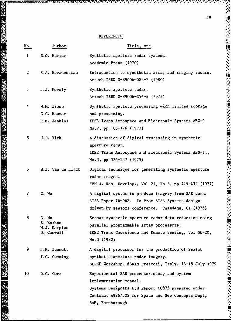
59
REFERENCES
No. Author Title, etc
I R.O. Harger Synthetic aperture radar systems.
Academic Press (1970)
2 S.A. Hovanessian Introduction to synethetic array and imaging radars.
Artech ISBN 0-89006-082-7 (1980)
3 J.J. Kovaly Synthetic aperture radar.
Artech ISBN 0-89006-G56-8 ('976)
4 W.M. Brown Synthetic aperture processing wich limited storage
G.G. Houser and presumming.
R.E. Jenkins IEEE Trans Aerospace and Electronic Systems AES-9
No.2, pp 166-176 (1973)
5 J.C. Kirk A discussion of digital processing in synthetic
aperture radar.
IEEE Trans Aerospace and Electronic Systems AES-Il,
No.3, pp 326-337 (1975)
6 W.J. Van de Lindt Digital technique for generating synthetic aperture
radar images.
IBM J. Res. Develop., Vol 21, No.5, pp 415-432 (1977)
7 C. Wu A digital system to produce imagery from SAR data.
AIAA Paper 76-968. In Proc AIAA Systems design
driven by sensors conference. Pasadena, Ca (1976)
8 C. Wu Seasat synthetic aperture radar data reduction usingB. BarkanW.J. Karplus parallel programmable array processors.
D. Caswell IEEE Trans Geoscience and Remote Sensing, Vol GE-20,
No.3 (1982)
9 J.R. Bennett A digital processor for the production of Seasat
I.G. Cumming synthetic aperture radar imagery.
SURGE Workshop, ESRIN Frascoti, Italy, 16-18 July 1979
10 D.G. Corr Experimental SAR processor.study and system
implementation manual.
Systems Designers Ltd Report C0875 prepared under
Contract A926/502 for Space and New Concepts Dept,
RAE, Farnborough
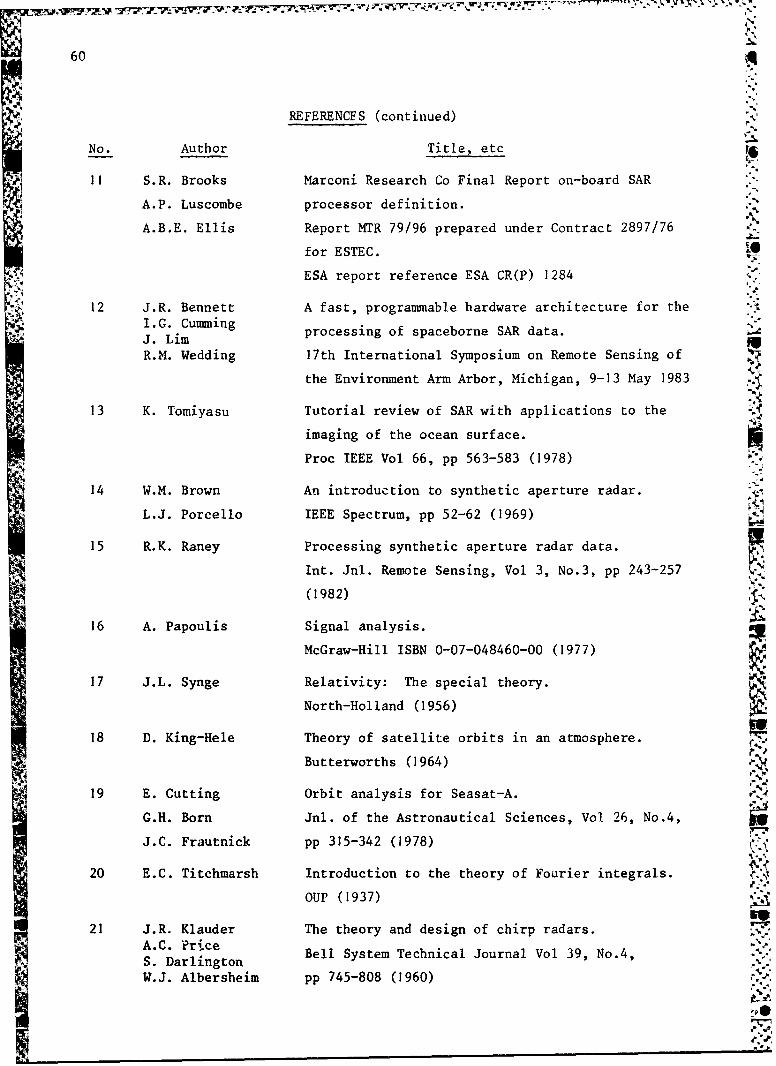
60
REFERENCFS (continued)vi•
No. Author Title, etc
11 S.R. Brooks Marconi Research Co Final Report on-board SAR
A.P. Luscombe processor definition.
A.B.E. Ellis Report MTR 79/96 prepared under Contract 2897/76
for ESTEC.
ESA report reference ESA CR(P) 1284
12 J.R. Bennett A fast, programmable hardware architecture for theI.G. Cumming processing of spaceborne SAR data.J. Lim f-R.M. Wedding 17th International Symposium on Remote Sensing of
the Environment Arm Arbor, Michigan, 9-13 May 1983
13 K. Tomiyasu Tutorial review of SAR with applications to the
imaging of the ocean surface.
Proc IEEE Vol 66, pp 563-583 (1978) 0
14 W.M. Brown An introduction to synthetic aperture radar.
L.J. Porcello IEEE Spectrum, pp 52-62 (1969)
15 R.K. Raney Processing synthetic aperture radar data.
Int. Jnl. Remote Sensing, Vol 3, No.3, pp 243-257
(1982)
16 A. Papoulis Signal analysis.
McGraw-Hill ISBN 0-07-048460-00 (1977)
17 J.L. Synge Relativity: The special theory.
North-Holland (1956)
18 D. King-Hele Theory of satellite orbits in an atmosphere.
Butterworths (1964) -
19 E. Cutting Orbit analysis for Seasat-A.
G.H. Born Jnl. of the Astronautical Sciences, Vol 26, No.4,
J.C. Frautnick pp 315-342 (1978)
20 E.C. Titchmarsh Introduction to the theory of Fourier integrals.
OUP (1937),Le
21 J.R. Klauder The theory and design of chirp radars.A.C. PrilceS.. Drligtoe Bell System Technical Journal Vol 39, No.4,S. Darlington
W.J. Albersheim pp 745-808 (1960)
:• 9*
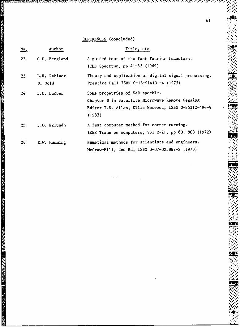
61
REFERENCES (concluded)
No. Author Title, etc
22 G.D. Bergland A guided tour of the fast Fourier transform.
IEEE Spectrum, pp 41-52 (1969)
23 L.R. Rabiner Theory and application of digital signal processing.
B. Gold Prentice-Hall ISBN 0-13-.914101-4 (1975)
24 B.C. Barber Some properties of SAR speckle.
Chapter 8 in Satellite Microwave Remote Sensing "__
Editor T.D. Allan, Ellis Horwood, ISBN 0-85312-494-9
(1983)
25 J.O. Eklundh A fast computer method for corner turning.IEEE Trans on computers, Vol C-21, pp 801-803 (1972)
26 R.W. Hamming Numerical methods for scientists and engineers.
McGraw-Hill, 2nd Ed, ISBN 0-07-025887-2 (1973)
Stp
'4 '. "
S:. ":'4%
*.- •'4
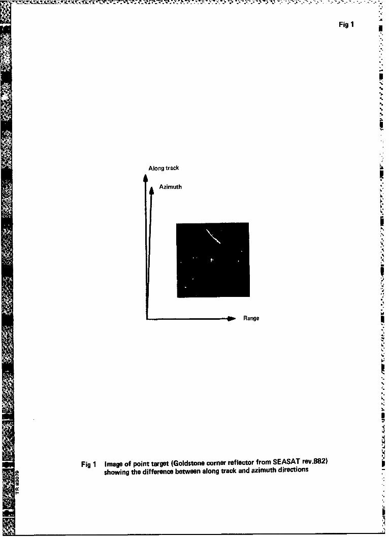
Fig 1
i.
Along track
Azimuth
OP Range
'I
Fig 1 Image of point target (Goldstone corner reflector from SEASAT rev.882)
showing the difference between along track and azimuth directionsCO40I..
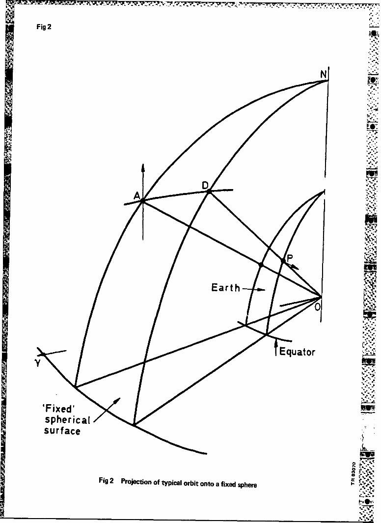
Fig 2
-- "~--F5
'Fixed'
NN
4-.•:
D4
A-
1-, "",
'Fixed'
spherical
Fig 2 Projection of typical orbit onto a fixed sphere .'-
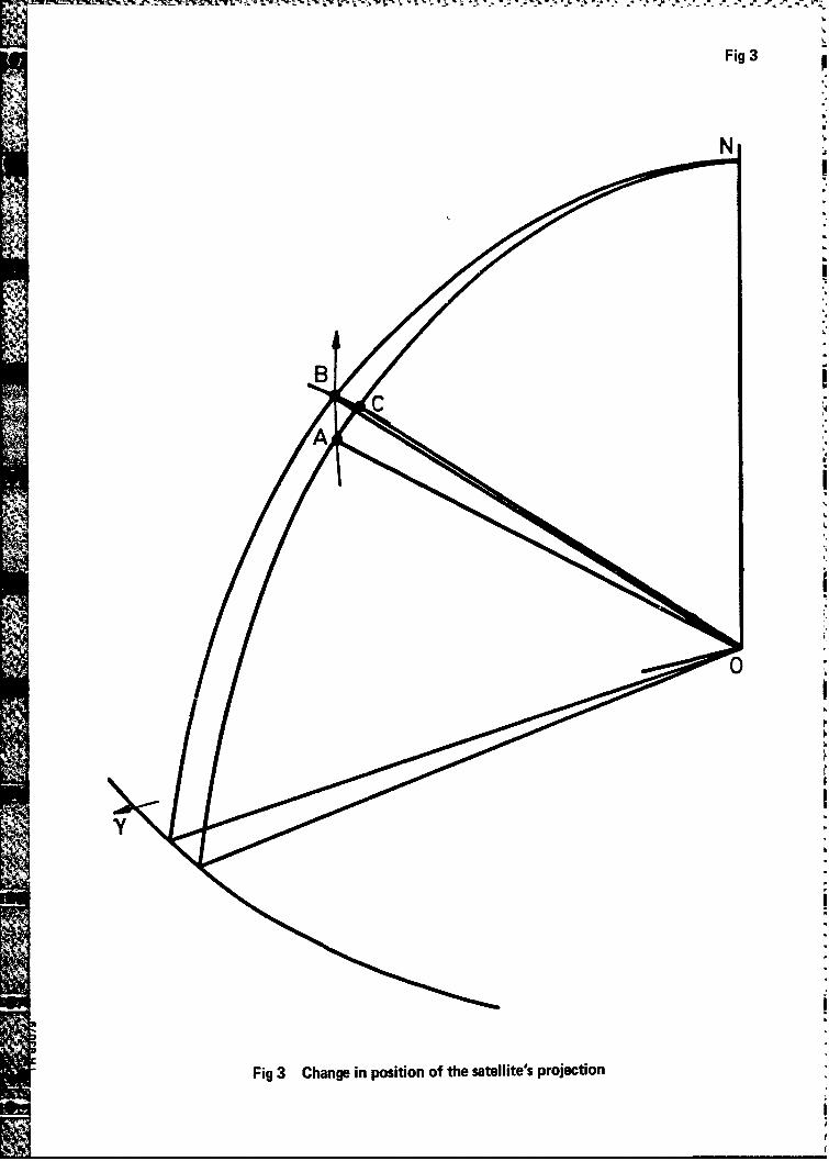
Fig 3
Fig 3 Change in position of the satellite's projection
IN
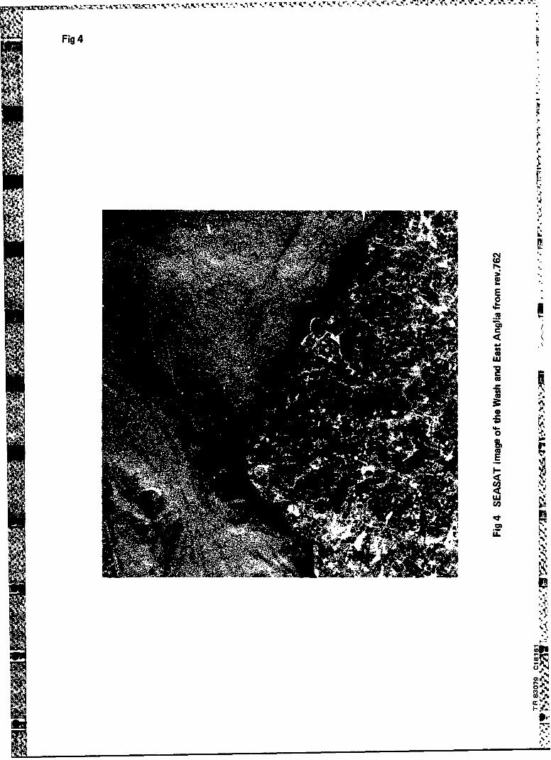
14 N
IL
Fig 4
LL.
1 0-
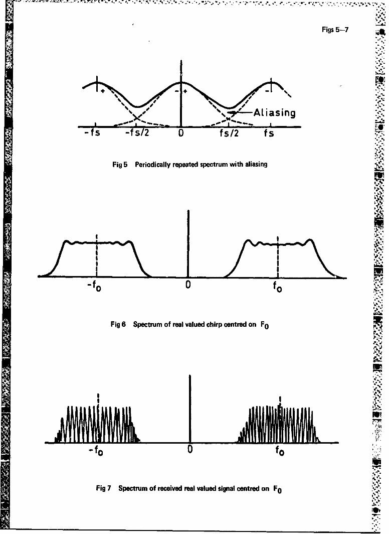
Figs 5-7 A
",Atiasing
-fs -f s/2 0fs/2 fS -
Fig 5 Periodically repeated spectrum with aliasing
Fig 6 Spectrum of real valued chirp centred on F0
'fo 0 fo
'4..
Fig 7 Spectrum of received real valued signal centred on F0
"414"
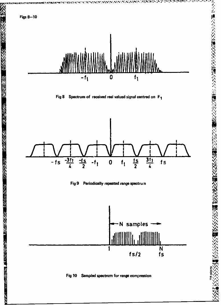
Figs 8-10
"UL
M,
tj•
Fig 8 Spectrum of received real valued signal centred on F1
M
-fs -3-f -f 0 s I fs2 2
Fig 9 Periodically repeated range spectruen
~.$
N samples -!
___________________________ ldllhllitlll.,i111111111111,
fs/2 fs
Fig 10 Sampled spectrum for range compression -'- .A ,
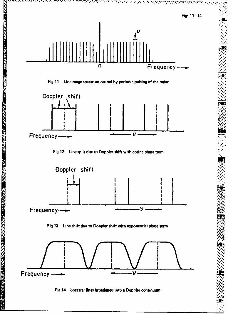
Figs 11- 14
n_ Frequency -...
Fig 11 Line range spectrum caused by periodic pulsing of the radar
Doppler shift t__
i 'i
II
Frequency- s. V -_
Fig 12 Line split due to Doppler shift with cosine phase term
Doppler shift,-,
\MT
Frequency-- - V
Fig 14 Spectral lines broadened into a Doppler continuum
-.4•
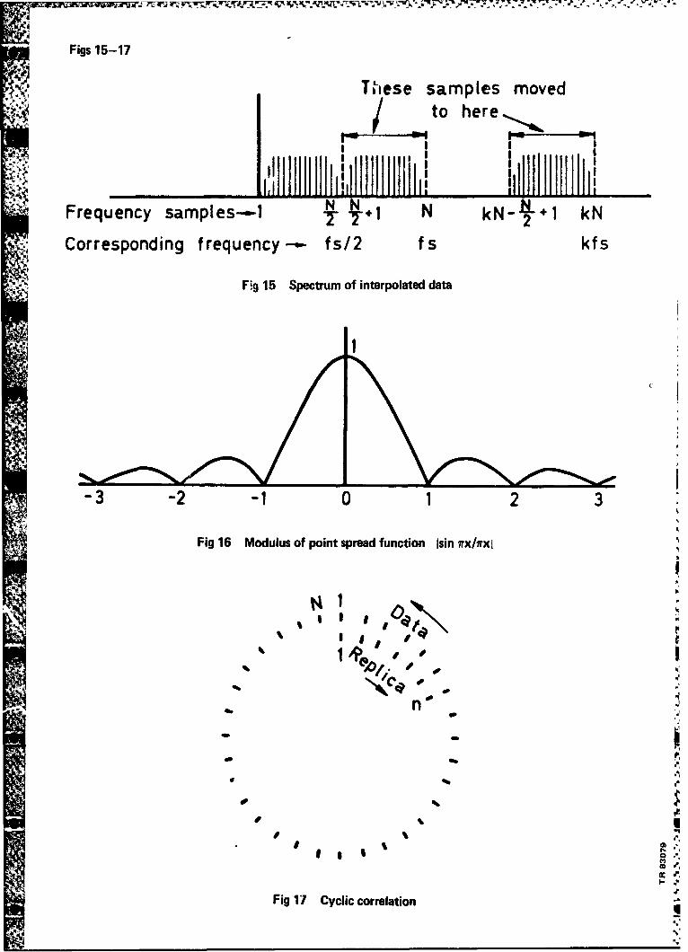
Figs 15-17
These samples moved-/ • to here
Frequency samples-e-1 N- N 1 N kN-4.l kN
Corresponding frequency-,- fs/2 fs kfs
Fig 15 Spectrum of interpolated data
-3 -2 -1 0 2 3
Fig 16 Modulus of point spread function Isin rx/wxl
Ii,', , ,o a
9.
%''
Fig 17 Cyclic correlation
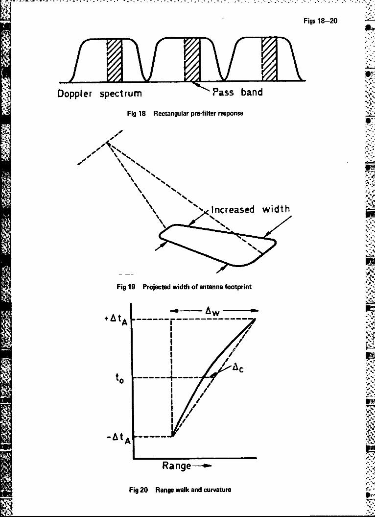
Figs 18-20
Doppler spectrum Pass band
Fig 18 Rectangular pre-filter response
+-A
A -- --
S\ %.
% %""x Increased width
4, ~AS~~~~Fig 20 PRangete walko andtennafoturen
IILw i k
II //'SIii/
I /
_AtAI ....---
S~~Range--
Fig 20 Range walk and curvature
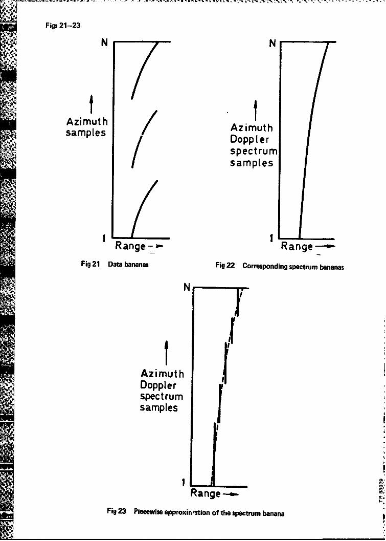
Figs 21-23
N N
- Azimuth
samples 7AzimuthDoppler/ cspectrumsamples
RaRange- x- R-a-nge -
Fig 21 Data bananas Fig 22 Corresponding spectrum bananas
Nr
Af AzimuthDopplerspectrumsamplesJ
Range-IFig 23 Piecewise approxini.,tion of the spectrum banana
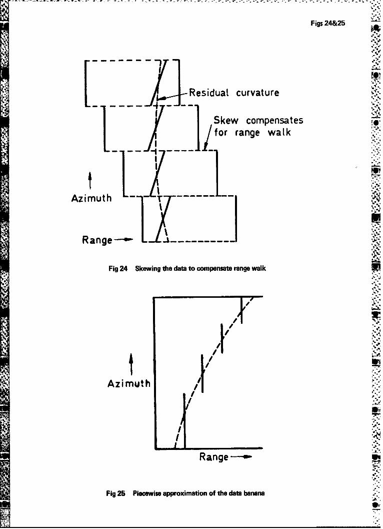
Figs 24&25
i• Residual curvature9%
"-1 '•--'-1 Skew compensates [9,SL-l --.....fo rag wl
_... ]. \... .....duaL
Range- L-L -,-
Fig 24 Skewing the data to compensate range walk
AzmuAzh uth
I I-
I IL I
RangeR
Fig 25 PSecewise approximation of the date banana
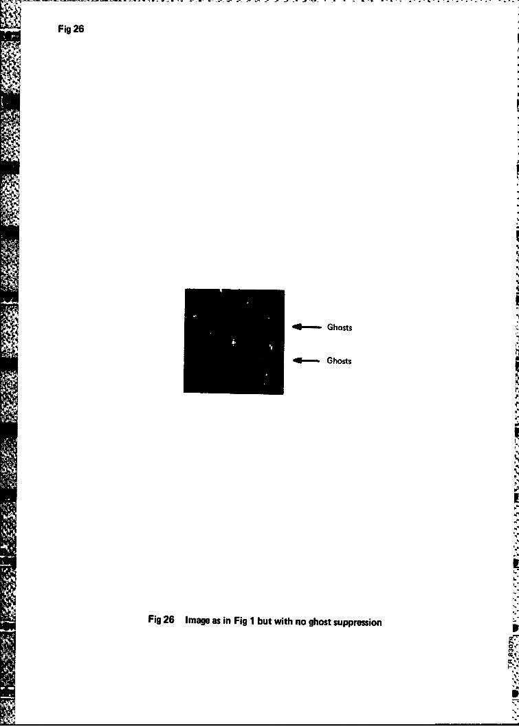
Fig 26N
44 - Ghosts
"41-- Ghosts
Fig 26 Image as in Fig 1 but with no ghost suppression
W*0"
ft.
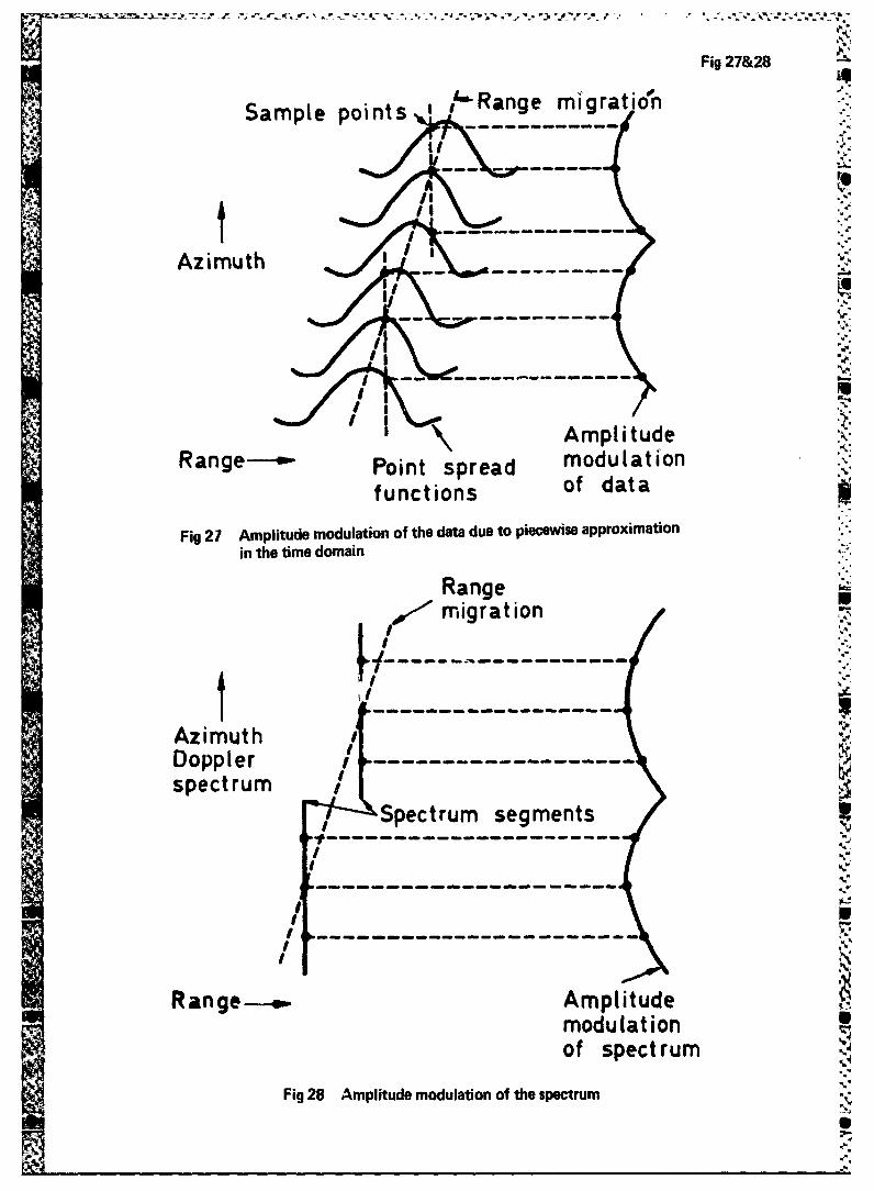
Fig 27&28
Sample points /-Range migrationS-----------
Azimuth-
-- - ---- n----
l 'I
AmplitudeRange---.-- Point spread modulationPit s r a of data
functions
Fig 27 Amplitude modulation of the data due to piecewise approximation
in the time domain
Range,/ ' migrat ion
Azimuth ........--------------
Doppler -------------------spectrum
sSpectrum segments
F I ~- --- ------------------
Range--. Amplitudemodulationof spect rum
Fig 28 Amplitude modulation of the spectrumI "
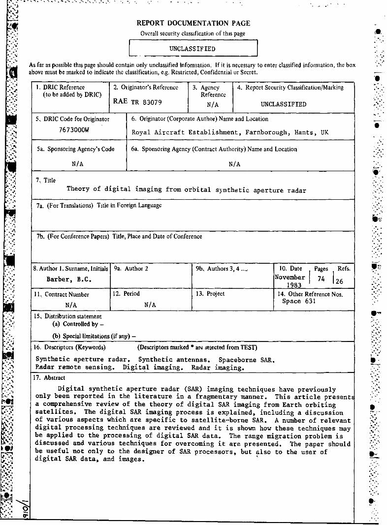
REPORT DOCUMENTATION PAGE
Overall security classification of this page
SLUNCLASSIFIEDI
As far as possible this page should contain only unclassified information. If it is necessary to enter classified information, the boxabove must be marked to indicate the classification, e.g. Restricted, Confidential or Secret.
1. DRIC Reference 2. Originator's Reference 3. Agency 4. Report Security Classification/Marking
(to be added by DRIC) ReferenceRAE TR 83079 NIA UNCLASSIFIED
5. DRIC Code for Originator 6. Originator (Corporate Author) Name and Location
7673000W Royal Aircraft Establishment, Farnborough, Hants, UK
5a. Sponsoring Agency's Code 6a. Sponsoring Agency (Contract Authority) Name and Location
N/A N/A
7, TitleTheory of digital imaging from orbital synthetic aperture radar
7a. (For Translations) Title in Foreign Language
7b. (For Conference Papers) Title, Place and Date of Conference
8. Author 1. Surname, Initials 9a. Author 2 9b, Authors 3,4 .......... 10. Date Pages Refs.
Barber, B.C. 1ueme 74 126___-__. " _1983
11. Contract Number 12. Period 13. Project 14. Other Reference Nos.SN/A N/A Space 631
15. Distribution statement(a) Controlled by -
(b) Special limitations (if any) -
16. Descriptors (Keywords) (Descriptors marked * ar% seiected from TEST)
Synthetic aperture radar. Synthetic antennas. Spaceborne SAR. SRadar remote sensing. Digital imaging. Radar imaging.
17. Abstract
Digital synthetic aperture radar (SAR) imaging techniques have previouslyC only been reported in the literature in a fragmentary manner. This article present '•'@1 a comprehensive review of the theory of digital SAR imaging from Earth orbiting
satellites. The digital SAR imaging process is explained, including a discussionof various aspects which are specific to satellite-borne SAR. A number of relevantdigital processing techniques are reviewed and it is shown how these techniques maybe applied to the processing of digital SAR data. The range migration problem isdiscussed and various techniques for overcoming it are presented. The paper shouldbe useful not only to the designer of SAR processors, but also to the user of
"'2 digital SAR data, and images.