8. L R OCAL ULES I E NFERRING NVIRONMENT … · approach was used with good results in modeling the housing market (Filatova ... complex markets such as the financial market (LeBaron

Romanian Journal of Economic Forecasting – 1/2012 128

LOCAL ENVIRONMENT ANALYSIS AND RULES INFERRING PROCEDURE IN AN AGENT-BASED MODEL – APPLICATIONS IN ECONOMICS

Andrei Silviu DOSPINESCU 1

Abstract

The use of agent-based modeling in economics is a step forward enabling a more realistic description of the complex interactions and behaviors occurring in the economic environment. Although it offers increased realism, especially in describing how local characteristics generate global patterns, it suffers from a simplistic approach to modeling local behaviors and rules. From this perspective the paper suggests possible solutions in two directions. First, the paper uses neural networks as an instrument for the agents to scan their local environment and infer possible behaviors. Second, the paper defines and applies an algorithm enabling the agents to understand a subset of rules that are not defined at the beginning of the application. The goal is to see how it is possible to generate new rules with structure and semantics. This would constitute “real” learning, namely defining new rules but not only quantitative variations of the initial rules. Keywords: agent-based modeling, neural networks, complex rules, algorithms JEL Classification: C15, C73, E37

1. Introduction

The structure and the modeling philosophy of the current macroeconomic models facilitate a rigorous statistical analysis, but they are not well equipped to analyze the effects of local behaviors of the economic agents, as well as the transition from local behavior to global patterns. These elements become fundamental, due to the complex propagation of the local behaviors in the current economy. In this context, there is a need for more realistic models capable of describing the complex structure and interactions in the economy (see Doney and Foley, 2009, for a convincing description of this issue). 1 Researcher at CISE, NIER, Romanian Academy, E-mail: [email protected].

This work was supported by the project "Post-Doctoral Studies in Economics: Training program for elite researchers - SPODE" co-funded from the European Social Fund through the Development of Human Resources Operational Programme 2007-2013, contract no. POSDRU/89/1.5/S/61755.

8.

Local Environment Analysis and Rules Inferring Procedure


The agent-based modeling approach seems to do a better job in this respect. The approach was used with good results in modeling the housing market (Filatova et al., 2007; Gilbert et al., 2008) and after 2008 the housing market crisis in the United States (Manhon and others, 2009), as well as the financial crisis (Thurner et al., 2009). More complex models were built for an in-depth description and analysis of complex markets such as the financial market (LeBaron, 2002). Currently, there is a rising interest in developing more ample models able to reflect in a more complex way the behaviors and evolution of the markets (see Doyne Farmer from Santa Fe Institute and Robert Axtell from George Mason University, http://www.santafe.edu/news/item/ could-better-models-foresee-economic-crises-farmer-axtell-geanakoplos/). The paper suggests two applications focusing on the autonomic behavior of agents in a simulation. From this perspective, it has two main objectives. The first one is to enable the agents to scan their local environment and infer their behavior on the basis of the data accumulated during the simulation. It must be stressed that in this case the decisions of the agents are not based on the inferences from the available information at the beginning of the simulation, for example, choosing the best strategies from a set of strategies (see de Araujo and Lamb 2008, Veit and Czernohous, 2003), but use “emergent” data, meaning data generated during the simulation. The second objective is to construct an algorithm that enables the agents to infer the characteristics of a subset of rules which are not defined by the modeler at the beginning of the application. The two objectives allows to build more flexible economic simulations in which the decisions of the economic agents are not based only on rules and information given at the beginning of the simulation, but also on information accumulated during the simulation of the economic model. In the second section we provide an overview of the model, focusing on the conceptual framework, the agents’ properties and behaviors and the model calibration. In the third section we focus on the way the agents scan their local environment and infer possible behaviors. An individual agent scans its local environment using a neural network and infers its behaviors in a new environment for which it has only partial information. Consequently, we present the building of the neural network and the results of the simulation. In the fourth section we present an algorithm that will enable the agents to infer the characteristics of rules unknown to them at the beginning of the simulation.

2. Overview of the model

The model describes a housing market with speculative and non-speculative agents2. The agents are placed on a lattice with 200 rows and 10 columns. There is an initial random distribution of the agents. The dynamics of the speculative and non-speculative behaviors is modeled using a neighborhood rule. Each agent has an initial price for the property which it intends to trade on the housing market. The dynamics of

2 The speculative agent is the agent whose price behavior is described by relation 2 and the

non-speculative agent is the agent whose price behavior is described by relation 1.

Institute for Economic Forecasting


prices is modeled using a specific function for speculative and non-speculative agents. The model does not have a complex structure, the housing market is used only as a framework for: 1) the analysis of the capacity of the agents to scan their local environment using neural network; and 2) proposing an algorithm that enables the agents to infer the characteristics of unknown rules. The paper focuses on the housing market due to previous work done by the author on modeling this market using agent-based models (Dospinescu, 2011). Consequently, the structure of the model reflects the objective of the paper; the focus is not on constructing an agent-based model and using it to analyze the housing market but on reflecting the capacity of the agents to use “emergent” information (information generated during the simulation) to infer their optimal behavior and on an algorithm which enables the agents to infer the characteristics of unknown rules. There is also not needed to replicate certain stylized facts, due to the objective of the paper, which is not focused on the analysis of the housing market, but on the behavior of the agents, as stressed above. The model is built and run using Visual Basic and Excel spreadsheets. Agent-based models use different platforms and programming languages. The same programming language was used by Macal and North (2007). Other platforms and programming languages are also used. For example, the model of Manhon and others (2009) runs on a NetLogo platform. LeBaron (2002) used a Swarm platform developed by the Santa Fe Institute. The agents In the simulation, the agents were placed on a lattice with 200 rows and 10 columns. Each element in the lattice has one of three states: s1, which corresponds to the non-speculative agents; s2, which corresponds to the speculative agents; and s3, which corresponds to an empty space. We define a probability space (S,F,P), where

{ }321 s,s,sS = . The probability of each state is given by p(s3)=c1, p(s3)=c2, p(s3)=c3, where the parameters c1, c2 and c3 reflect the probabilities of s1, s2 and s3 in the lattice. An initial population was generated with probabilities 0.35, 0.35 and 0.3, respectively (see Figure 1).

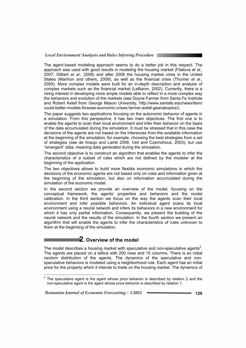
Figure 1 The initial distribution of agents on the lattice



Legend: The light colored (yellow spaces) represent the non-speculative agents, the darken colored (blue spaces) represent speculative agents and the white represent the empty spaces. The lattice is obtained based on the procedure outlined above (see “The agents”). Source: Own computations.

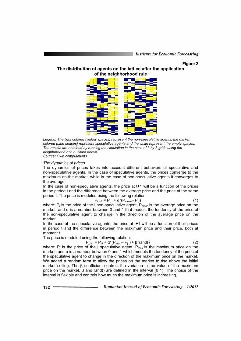
We have chosen these probabilities to underline the effect of the neighborhood rule. If one of the states was dominant; for example, the speculative agents were dominant, then it was intuitively clear that the application of the neighborhood rule would generate a simple pattern where the speculative agents would become the only type of agents (see the neighborhood rule for more details). The procedure populates a lattice with 200 rows and 10 columns with speculative agents, non-speculative agents and a number of empty spaces. The neighborhood rule The dynamics of the population of speculative and non-speculative agents can be modeled in different ways. In Dospinescu (2011) it was modeled using a game theory type of matrix and the transition of the population from one state to the other was based on the dynamic multiplayer proposed by Taylor and Jonker (1978). This approach allows for the analysis of the impact of incentives to speculate and not to speculate on the number of speculative and non-speculative agents. In this paper, we are interested in analyzing deeper the impact of local rules of interactions. This is why a neighborhood rule was chosen to model the dynamics in the population of agents. For each 3 by 3 and 6 by 6 grid the dominant behavior becomes the only behavior on that grid. This is similar to say that the dominant behavior is diffused in the local environment. This approach stresses the impact of limited local interactions on the dynamics of the global environment. The power of this approach is only partially used in this application, due to the different focus of this paper. Nonetheless, it is worth noticing that the complex global behaviors can be generated by simple local rules (see Gardner 1970 for a compelling argument in this respect). Running the simulation in the case of 3 by 3 grids we obtained a result that reflected the effect of the neighborhood rule, namely only one dominant behavior on each grid (see Figure 2). In the third and the fourth sections of the paper we applied the neighborhood rule to a 3 by 3 grid. We have chosen this approach due to the more complex patterns obtained in this case for the lattice of speculative and non-speculative agents. We also simulated for 6 by 6 grids in three different cases: 1) no common agents between grids; 2) six common agents; 3) twelve common agents. The simulation illustrated an intuitive result, namely the higher the number of common agents, the higher the diffusion of a behavior from region to region. For example, in the case of twelve common agents the dominant type of agents at the beginning of the simulation (from the higher region of the lattice) became the only type of agents in the lattice.



Figure 2 The distribution of agents on the lattice after the application

of the neighborhood rule

Legend: The light colored (yellow spaces) represent the non-speculative agents, the darken colored (blue spaces) represent speculative agents and the white represent the empty spaces. The results are obtained by running the simulation in the case of 3 by 3 grids using the neighborhood rule outlined above. Source: Own computations

The dynamics of prices The dynamics of prices takes into account different behaviors of speculative and non-speculative agents. In the case of speculative agents, the prices converge to the maximum on the market, while in the case of non-speculative agents it converges to the average. In the case of non-speculative agents, the price at t+1 will be a function of the prices in the period t and the difference between the average price and the price at the same period t. The price is modeled using the following relation: Pi,t+1 = Pi, t + α*(Pmean - Pi,t) (1) where: Pi is the price of the i non-speculative agent, Pmean is the average price on the market, and α is a number between 0 and 1 that models the tendency of the price of the non-speculative agent to change in the direction of the average price on the market. In the case of the speculative agents, the price at t+1 will be a function of their prices in period t and the difference between the maximum price and their price, both at moment t. The price is modeled using the following relation: Pj,t+1 = Pj,t + α*(Pmax – Pj,t) + β*rand() (2) where: Pj is the price of the j speculative agent, Pmax is the maximum price on the market, and α is a number between 0 and 1 which models the tendency of the price of the speculative agent to change in the direction of the maximum price on the market. We added a random term to allow the prices on the market to rise above the initial market ceiling. The β coefficient controls the variation in the value of the maximum price on the market. β and rand() are defined in the interval (0 1). The choice of the interval is flexible and controls how much the maximum price is increasing.



The migration rule

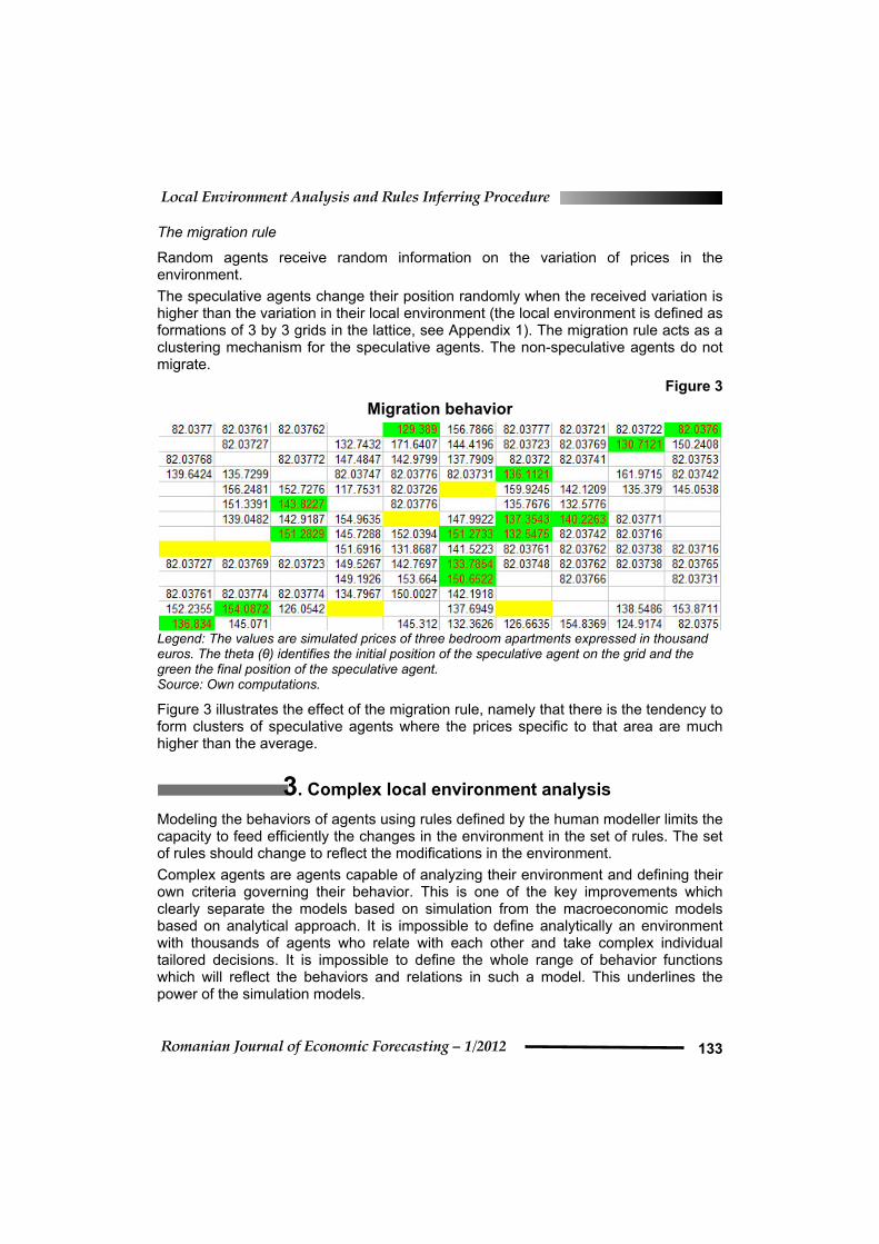
Random agents receive random information on the variation of prices in the environment. The speculative agents change their position randomly when the received variation is higher than the variation in their local environment (the local environment is defined as formations of 3 by 3 grids in the lattice, see Appendix 1). The migration rule acts as a clustering mechanism for the speculative agents. The non-speculative agents do not migrate.

Figure 3 Migration behavior

Legend: The values are simulated prices of three bedroom apartments expressed in thousand euros. The theta (θ) identifies the initial position of the speculative agent on the grid and the green the final position of the speculative agent. Source: Own computations.

Figure 3 illustrates the effect of the migration rule, namely that there is the tendency to form clusters of speculative agents where the prices specific to that area are much higher than the average.

3. Complex local environment analysis

Modeling the behaviors of agents using rules defined by the human modeller limits the capacity to feed efficiently the changes in the environment in the set of rules. The set of rules should change to reflect the modifications in the environment. Complex agents are agents capable of analyzing their environment and defining their own criteria governing their behavior. This is one of the key improvements which clearly separate the models based on simulation from the macroeconomic models based on analytical approach. It is impossible to define analytically an environment with thousands of agents who relate with each other and take complex individual tailored decisions. It is impossible to define the whole range of behavior functions which will reflect the behaviors and relations in such a model. This underlines the power of the simulation models.



The ample structure of interactions between the agents ensures the complex behavior of the global system of agents. Nonetheless, a more realistic model would incorporate agents capable of complex analysis of their environment. In this respect, there is a relevant point to stress out. Simple neighborhood rules are useful and enable, for example, the cellular automata to analyze complex contexts. Nonetheless, each component in the cellular automata is not capable to analyze the environment, and only by their collective behavior is such a property obtained. Consequently, each agent in an agent-based model is not able to analyze its environment by simple neighborhood rules. This is possible only if each agent acts as a cellular automaton. Agent-based models are starting to use complex algorithms which enable the agents to take decisions and improve their behavior. In this respect, LeBaron (2002) used genetic algorithms as a means to select the most fitted rules to improve the decisions made by the agents. Nonetheless, it is worth noticing that in this case the agents are not actually analyzing the environment, but are identifying the most fitted rules based on feed-back from the environment. Another promising approach is the neural network based agents (NNBA). Applications are mainly in informatics: Machado, V.; Neto, A.; de Melo, J.D. (2010), Ray Eberts and Shidan Habibi (1995), Charles C. Willow (2005), and engineering: Arefin, Alom and Saha (2009), Quirolgico, Camfield, Finin and Smith (1999). In economics this approach is still less used. This is mainly due to the mainstream macroeconomic modeling approaches deeply rooted in the economic analyses. In economics, the application of this approach is suited to environments with large quantities of data structured by different criteria, which are generated by the interactions of a large group of agents. From this respect, NNBA are used, for example in Veit and Czernohous (2003). The authors compare the results obtained from rule-based agents and NNBA in identifying the best possible strategies on the energy market. In this case, the neural network was used to select the best strategy from a set of possible strategies. The agents are not analyzing the environment, but they are selecting the best-fitted strategies. An approach related to the above one is that of de Araujo and Lamb (2008), which uses the neural networks to analyze the best possible strategies. The objective is to see if the choices lead to a Nash equilibrium strategy matrix. Neural networks are used to improve the agents’ strategies or to reflect the pattern of economic data. Nonetheless, the real economic agents define their strategies on the basis of the economic environment. The important point stressed here is the capacity to analyze the environment and define strategies based on that analysis. In comparison with Veit and Czernohous (2003) and de Araujo and Lamb (2008), our model is not based on the information available to the agents at the beginning of the simulation, but on the information that is generated during the simulation. This allows for a more flexible behavior of agents in an economic model. The modeling strategy proposed in this paper is based on the following steps: 1. The model runs the procedures for: 1) the interactions of agents based on the

neighborhood rule (see Figure 2); 2) the dynamics of prices based on the specific functions for the speculative and non-speculative agents; 3) the migration of speculative agents (see Ffigure 3);



2. An individual agent evaluates the environment using a neural network with nine inputs, three neurons in the hidden layer and one output neuron. The model is based on a supervised neural network, which is trained using as inputs the prices of the agents on 3 by 3 grids and as an output the number of speculative agents on 3 by 3 grids. The training data is represented by the prices and the number of speculative agents specific to a total of 25 three by three grids. This is equivalent with a training set described by a matrix with 10 rows and 25 columns. The training of the neural network simulates the inferences made by an agent using the known data available to him;

3. The individual agent moves to an unknown area in which it has information only about the prices on the local market;

4. The individual agent uses the neural network to infer if the unknown area is dominated by speculative or non-speculative agents. If the individual agent moves in an area compatible with it (for example, dominated by non-speculative agents if it is non-speculative) then it remains in that area, if not it moves to the other local areas until it finds a compatible one.

The important element to be stressed in this case is that the relation between the prices and the number of agents is inferred by the individual agent, and if the relation changes due to the evolution of the environment the individual agent adapts to the changes and takes different decisions. In training the neural network, we used a back propagation algorithm. The transfer function is a sigmoid function. We have chosen an algebraic function

xx)x(f

+=

1,

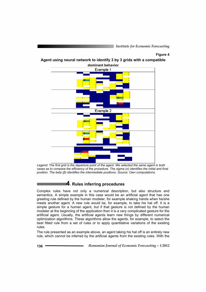
which enables a more clear distinction between the high and the low values of inputs than other sigmoid functions. We selected the same non-speculative agent in both cases (examples 1 and 2) to compare the efficiency and the stability of the procedure. The agent uses the trained neural network to move on different 3 by 3 grids and feed the prices from that grid to the neural network. The output of the neural network gives an estimate of the number of speculative agents. If the number of speculative agents is dominant, then the agent moves to a different grid, otherwise it remains in that grid. Figure 4 shows that the agent was able to move from grid to grid until he/she has found a grid dominated by non-speculative agents. As one may see in example 2, the agent left an intermediate grid (see the second row of the second table), which was dominated by non-speculative agents. The efficiency of the neural network depends on the differences in prices between the speculative and non-speculative agents. If the prices in a grid are higher than expected for non-speculative agents then the non-speculative agent leaves that grid. The procedure illustrated in Figure 4 demonstrates the use of neural network by agents, who take decisions based on the patterns occurring in their environment. The main advantage of this procedure is the capacity of agents to take complex decisions based not on the rules defined by the human modeller at the beginning of the application but on the simulated environment.



Figure 4 Agent using neural network to identify 3 by 3 grids with a compatible

dominant behavior

Legend: The first grid is the departure point of the agent. We selected the same agent in both cases as to compare the efficiency of the procedure. The sigma (σ) identifies the initial and final position. The beta (β) identifies the intermediate positions. Source: Own computations.

4. Rules inferring procedures

Complex rules have not only a numerical description, but also structure and semantics. A simple example in this case would be an artificial agent that has one greeting rule defined by the human modeler, for example shaking hands when he/she meets another agent. A new rule would be, for example, to take his hat off. It is a simple gesture for a human agent, but if that gesture is not defined by the human modeler at the beginning of the application then it is a very complicated gesture for the artificial agent. Usually, the artificial agents learn new things by different numerical optimization algorithms. These algorithms allow the agents, for example, to select the best fitted rule from a set of rules or to apply quantitative variations of the existing rules. The rule presented as an example above, an agent taking his hat off is an entirely new rule, which cannot be inferred by the artificial agents from the existing rules. With the



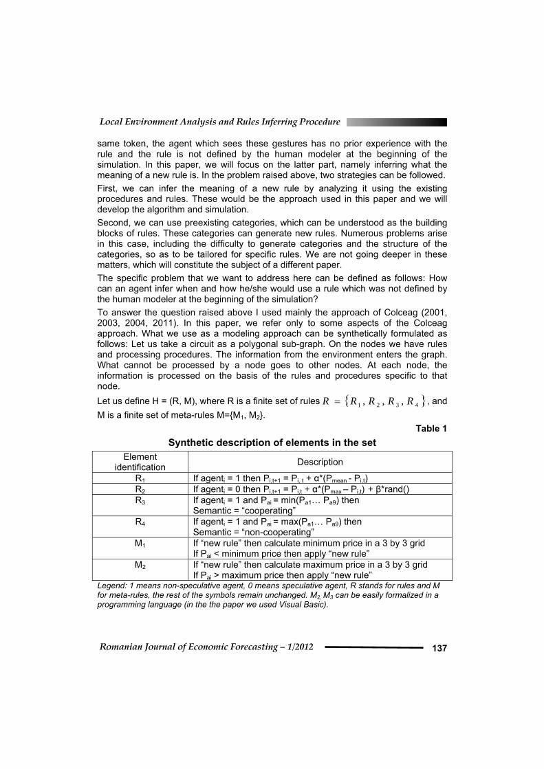
same token, the agent which sees these gestures has no prior experience with the rule and the rule is not defined by the human modeler at the beginning of the simulation. In this paper, we will focus on the latter part, namely inferring what the meaning of a new rule is. In the problem raised above, two strategies can be followed. First, we can infer the meaning of a new rule by analyzing it using the existing procedures and rules. These would be the approach used in this paper and we will develop the algorithm and simulation. Second, we can use preexisting categories, which can be understood as the building blocks of rules. These categories can generate new rules. Numerous problems arise in this case, including the difficulty to generate categories and the structure of the categories, so as to be tailored for specific rules. We are not going deeper in these matters, which will constitute the subject of a different paper. The specific problem that we want to address here can be defined as follows: How can an agent infer when and how he/she would use a rule which was not defined by the human modeler at the beginning of the simulation? To answer the question raised above I used mainly the approach of Colceag (2001, 2003, 2004, 2011). In this paper, we refer only to some aspects of the Colceag approach. What we use as a modeling approach can be synthetically formulated as follows: Let us take a circuit as a polygonal sub-graph. On the nodes we have rules and processing procedures. The information from the environment enters the graph. What cannot be processed by a node goes to other nodes. At each node, the information is processed on the basis of the rules and procedures specific to that node. Let us define H = (R, M), where R is a finite set of rules { }4321 ,,, RRRRR = , and M is a finite set of meta-rules M={M1, M2}.

Table 1 Synthetic description of elements in the set

Element identification Description

R1 If agenti = 1 then Pi,t+1 = Pi, t + α*(Pmean - Pi,t) R2 If agenti = 0 then Pi,t+1 = Pi,t + α*(Pmax – Pi,t) + β*rand() R3 If agenti = 1 and Pai = min(Pa1… Pa9) then

Semantic = “cooperating” R4 If agenti = 1 and Pai = max(Pa1… Pa9) then

Semantic = “non-cooperating” M1 If “new rule” then calculate minimum price in a 3 by 3 grid

If Pai < minimum price then apply “new rule” M2 If “new rule” then calculate maximum price in a 3 by 3 grid

If Pai > maximum price then apply “new rule” Legend: 1 means non-speculative agent, 0 means speculative agent, R stands for rules and M for meta-rules, the rest of the symbols remain unchanged. M2, M3 can be easily formalized in a programming language (in the the paper we used Visual Basic).



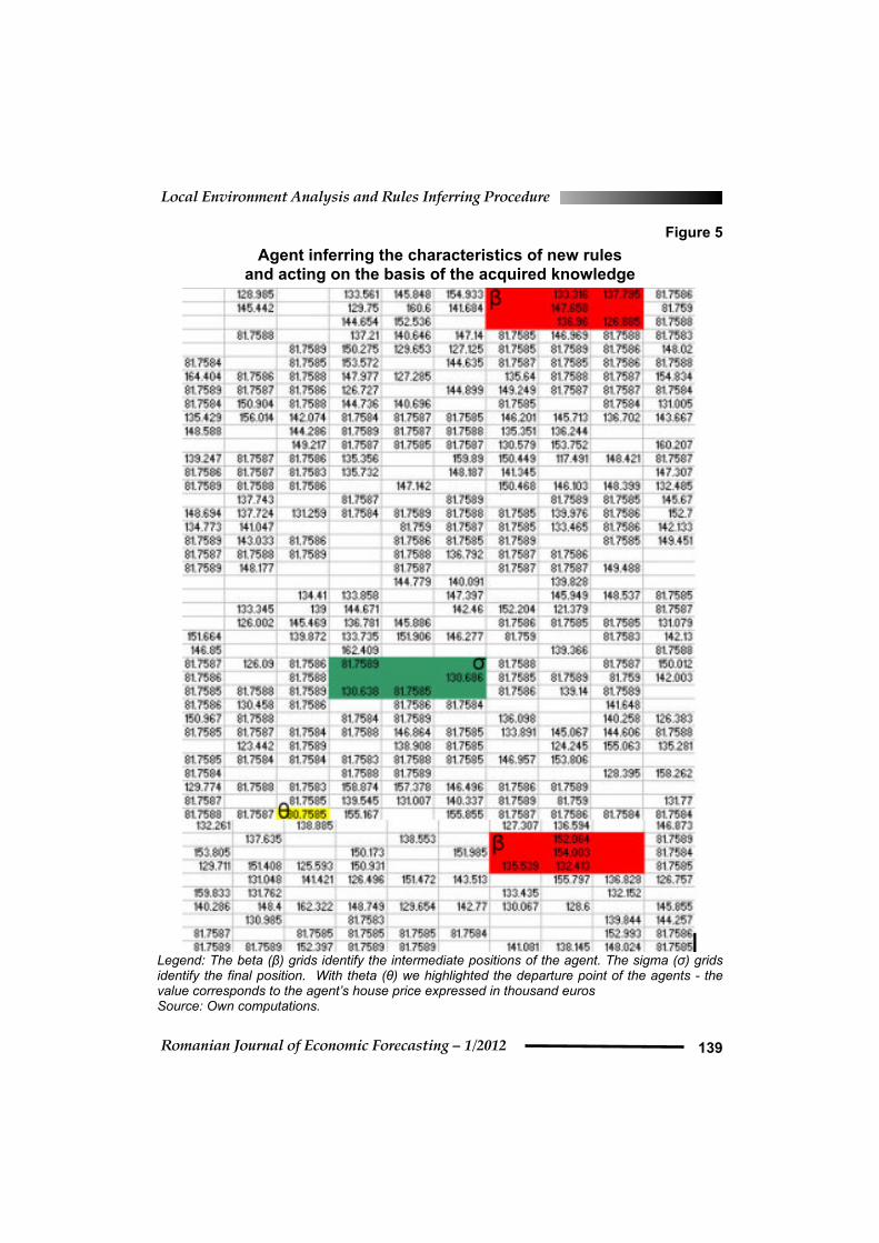
Let ai be a non-speculative agent who applies rules R1 and meta-rules M1 and M2 and does not apply R2, R3 and R4. Let agent ai be the only agent not applying rules R3 or R4. The agent knows from M1 and M2 that the application of a new rule can be inferred by calculating the minimum and the maximum of prices on 3 by 3 grids. He/she proceeds to analyze different grids and see if it has a smaller or a higher price than the minimum or the maximum price on that grid. If he/she finds such a grid, it stops and moves to that grid. He/she uses the new rule, which is applied by the agent with the minimum price on that grid if he/she has a price smaller than the minimum price on that grid or the new rule applied by the agent with a maximum price on that grid if he/she has a price higher than the maximum price on that grid. Ideally, it should apply R3 because it is a non-speculative agent. This suggests that learning a new rule is based on inferences from the environment in which the agent is immersed. The perspective is consistent with the attribution theory, which “deals with how the social perceiver uses information to arrive at causal explanations for events. It examines what information is gathered and how it is combined to form a causal judgment” (see Fiske and Taylor, 1991). This is also the case of agent ai, who gathers data from the environment and behaves according to the data available to him/her. The result of the simulation is shown in Figure 5. The agent whose behavior is analyzed is light colored (yellow spaces). The beta grids correspond to the grids analyzed by the agent. The sigma grid corresponds to the position to which the agent has moved. The agent tests if on the highlighted grids it has a price higher or lower than the maximum or minimum price on that grid. He/she moves to the sigma grid because he/she has the minimum price on that grid and applies R3, which is consistent with the behavior of a non-speculative agent. The application of relations (1) and (2) makes very difficult for a non-speculative agent to have the maximum price on a grid. If he/she would have had a maximum price on a highlighted grid, then he/she would have applied R4, which would have been inconsistent with him/her being a non-speculative agent.



Figure 5 Agent inferring the characteristics of new rules

and acting on the basis of the acquired knowledge

Legend: The beta (β) grids identify the intermediate positions of the agent. The sigma (σ) grids identify the final position. With theta (θ) we highlighted the departure point of the agents - the value corresponds to the agent’s house price expressed in thousand euros Source: Own computations.



5. Conclusions and further developments

In this paper I focused on two main ideas. First, I illustrated the capacity of agents to take complex decisions based not on the rules defined by the human modeller at the beginning of the application, but on the simulated environment. This was done by training a neural network to identify the relation between the level of prices and the number of speculative agents. The neural network was used by the agent to find the areas which are compatible with it. As I pointed out, the important advantage of this approach is that the relation between the prices and the number of agents is inferred by the individual agent. If the relation changes due to the evolution of the environment, the individual agent adapts to the changes and takes different decisions. Second, I suggested an algorithm that allowed the agent to infer the characteristics of the rules that were not defined by the modeler at the beginning of the application and acted on the basis of these inferred characteristics. The algorithm is tested and the results are illustrated in Figure 5. The agent is capable to learn successfully the new rule and act according to it. Further developments on this line will focus on the complex task of defining algorithms that allow the agents to define rules with structure and semantics. One possible direction would be to use preexisting categories that can be understood as the building blocks of rules. Another possible direction is algebraic fractals (see Colceag, 2001). We are slowly entering an area where scientific reasoning begins to be strongly connected with the sensibility of the modeler and his/her capacity to understand intimately the instruments used and the implications of his/her results on the environment under study.

References

Colceag, F., 2001. Cellular automata; algebraic fractals. Available at: <http://austega.com/florin/CellularAutomataAlgebraicFractals.htm> [Accessed on 24 February 2011].

Colceag, F., 2003. Informational fields, structural fractals. Available at: <http://austega.com/florin/INFORMATIONAL%20FIELDS.htm> [Accessed on 24 February 2011].

Colceag, F., 2004. The universal language. Available at: <http://austega.com/florin/univlang/THE%20UNIVERSAL%20LANGUAGE%20-%20engl.html> [Accessed on 24 February 2011].

Colceag, F., 2011. Fractal completeness philosophy of the alive universe, Lattice Automata. Available at <http://www.sustainability-modeling.eu/media/ Fractal_completeness_philosophy _of_the_alive_universe.pdf> [Accessed on 24 February 2011].

de Araujo, R.M. and Lamb, L.C., 2004. “Neural Evolutionary Learning in a Bounded Rationality Scenario”, in Proceedings of the 11th International Conference, ICONIP 2004, Calcutta, India.



Dospinescu, A.S., 2011. “Analyzing the dynamics of relative prices on a market with speculative and non-speculative agents based on an evolutionary model”. Romanian Journal of Economic Forecasting, 14(1), pp. 72-87.

Eberts, R. and Shidan, H.,1995. “Neural network-based agents for integrating information for production systems”, International Journal of Production Economics, 38 (1), pp. 73-84

Farmer, J Doney and Foley, D., 2009. “The economy needs agent-based modeling”. Nature, 460, pp. 685-686.

Filatova, T. van der Veen, A. and Parker, D. C., 2007. Modeling of a residential land market with a spatially explicit agent-based land market model (ALMA). The 2nd Workshop of Market Dynamics SIG.

Fiske, S.T. and Taylor, S.E., 1991. Social cognition. New York: McGraw-Hill. Gardner, M. 1970. “Game of life”. Scientific American, October, ISBN 0894540017. Gilbert, N. Hawksworth, J.C. and Sweeney, P., 2008. An Agent-based Model of the

UK Housing Market. Available at: <http://cress.soc.surrey.ac.uk/ housingmarket/ukhm.html> [Accessed on 10 February 2011].

Arefin, K.S. Emdad, A. and Zahangir, A., 2008. “Cross-Layer Design of Wireless Networking for Parallel Loading of Access Points and Mirrored Servers (APMS)”. in Proceedings of International Conference on Electronics, Computer and Communications (ICECC 2008), June 27-29, 2008, Rajshahi, Bangladesh.

Le Baron, B., 2002, Building the Santa Fe Artificial Stock Market. Available at <http://www2.econ.iastate.edu/tesfatsi/blake.sfisum.pdf> [Accessed on 11 February 2011]

Machado, V. Neto, A. and de Melo, J.D., 2010. “A Neural Network Multiagent Architecture Applied to Industrial Networks for Dynamic Allocation of Control Strategies Using Standard Function Blocks”. Industrial Electronics, 57(5), pp. 1823-1834.

McMahon, M., Berea, A. and Hoda O., 2009. An Agent-Based Model of the Housing Market. Available at <http://www.css.gmu.edu/images/ HousingMarket_revisited/Housing_Market_revisited.pdf> [Accessed on 10 February 2011].

Santa Fee Institute, 2010. Rethinking economics: Could better models foresee economic crises?. Available at <http://www.santafe.edu/news/item/could-better-models-foresee-economic-crises-farmer-axtell-geanakoplos/> [Accessed on 16 February 2011].

Taylor, P.D. and Jonker, L.B., 1978. “Evolutionary Stable Strategies and Game Dynamics”. Mathematical Biosciences, 40, pp. 145–156.

Thurner S., Farmer, J. D. and Geanakoplos, J., 2009. Leverage Causes Fat Tails and Clustered Volatility, available at: <http://www.santafe.edu/media/workingpapers/09-08-031.pdf> [Accessed on 10 February 2011].



Veit D., and Czernohous, C., 2003. “Automated Bidding Strategy Adaption using Learning Agents in Many-to-Many e-Markets”. in: Poster Proceedings of the Workshop on Agent Mediated Electronic Commerce V (AMEC-V), held at the Second International Joint Conference on Autonomous Agents and Multi-Agent Systems (AAMAS), Melbourne.

Quirolgico, Camfield, Finin and Smith, 1999. Merging Neural Networks in a Multi-Agent System. Available at: <http://www.cs.umbc.edu/courses/pub/finin/papers/drafts/aaai2000.pdf> [Accessed on 10 February 2011].

Willow, Charles C. 2005. “A Neural Network-Based Agent Framework for Mail Server Management”. International Journal of Intelligent Information Technologies 1(4), pp. 36-52



Appendix 1

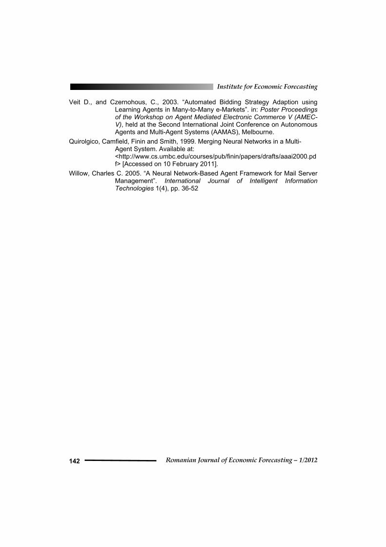
Table A.1 Synthetic presentation of the model

Agents Two types of agents, speculative and non-speculative. The distribution of the agents on the lattice is based on the probabilities c1 and c2 (see “The agents”)

Components of the model

Prices Each agent has an initial price for the property which he/she intends to trade on the housing market. Prices are generated using a uniform distribution (see Dospinescu, 2011). The dynamics of prices is modeled using specific function for speculative and non-speculative agents (see relations 1 and 2, respectively). Populating the lattice In the simulation, the agents were placed on a lattice with 200 rows and 10 columns. Each element in the lattice has one of three states: s1, which corresponds to the non-speculative agents, s2, which corresponds to the speculative agents and s3, which corresponds to an empty space. We define a probability space (S,F,P), where: { }321 ,, sssS = . The probability of each state is given by p(s3)=c1, p(s3)=c2, p(s3)=c3, where the parameters c1, c2 and c3 reflect the probabilities of s1, s2 and s3 in the lattice. Applying the neighborhood rule For each 3 by 3 grid in the lattice the dominant behavior becomes the only behavior on that grid. This is similar to say that the dominant behavior diffuses in the local environment (see Figures 1 and 2). The dynamics of prices In the case of the non-speculative agents the price is modeled using relation 1 In the case of the speculative agents, the price in modeled using relation 2.

Specifications

The migration rule Random agents receive random information on the variation in prices from the environment. The speculative agents migrate when the received variation is higher than the variation in their local environment. The migration rule acts as a clustering mechanism for the speculative agents. The non-speculative agents do not migrate.

Local environment

analysis

We build a neural network with nine inputs, three neurons in the hidden layer and one output neuron. The neural network is trained to identify the relation between the level of prices and the number of speculative agents in local environments which is described using 3 by 3 grids. An individual agent evaluates the environment using a neural network Then he/she moves to an unknown area in which he/she has information only about the prices on the local market. Using the neural network he/she infers if the unknown area is dominated by speculative or non-speculative agents. If the individual agent moves in an area compatible with him/her then he/she remains in that area, if not he/she moves to the other local areas until he/she finds one which is compatible.

Documents

8. L R OCAL ULES I E NFERRING NVIRONMENT … · approach was used with good results in modeling the housing market (Filatova ... complex markets such as the financial market (LeBaron