Transport processes

7. Semester

Chemical Engineering

Civil Engineering

Course plan

1. Elementary Fluid Dynamics2. Fluid Kinematics3. Finite Control Volume Analysis4. Differential Analysis of Fluid Flow5. Viscous Flow and Turbulence6. Turbulent Boundary Layer Flow7. Principles of Heat Transfer8. Internal Forces Convection9. Unsteady Heat Transfer10. Boiling and Condensation11. Mass Transfer12. Porous Media Flow13. Non-Newtonian Flow

Today's lecture

• Turbulent Boundary layer flow– Blasius solution

– Momentum Integral Analysis

– The regions of the turbulent boundary layer

Boundary layer characteristics

• Boundary layer thickness

( ) for 0.99y u y Uδ = =

5Re 2 10cr = ×

Boundary layer thickness

01 u dy

Uδ

∞∗ = − ∫

Standard boundary layer thickness

Displacement thickness Momentum thickness

01u u dy

U Uθ

∞ = − ∫( ) for 0.99y u y Uδ = =

Wall shear stress

• Given your knowledge of velocity profiles, explain the development of the wall shear stress

• Use two minutes to discuss with the person next to you

Boundary layer equations

• Simplified Navier-Stokes equations– Flow is parallel to the plate

– Flow is 2 dimensional

– Fluid is convected downstream more quickly then it diffuses across the streamlines

2

2

0u vx y

u u uu vx y y

µρ

∂ ∂+ =

∂ ∂

∂ ∂ ∂+ =

∂ ∂ ∂

From continuity

From x-,y-NS-equations, pressure eliminated

Only the largest terms are retained

Boundary conditions

• The boundary condition between the b.layer and the wall:

• The boundary condition between the b.layer and the free flow:

0 0u v for y= = =

0.99u U for y δ= =

‘no slip’ BC

Blasius solution

“The mathematical details of the solution are quite tedious and complex and will not be given here” - Geankoplis.

“In general, the solutions of nonlinear partial differential equations are extremely difficult to obtain.” - Munson et al.

Blasius solution – the result!

• The boundary thickness grows with the square root of the distance from the leading edge

• The wall shear stress decreases with increasing boundary layer thickness

5 xUµδρ

=

5Rexx

δ= 1.721

Rexxδ ∗

=0.664

Rexxθ=

3 20.332w Uxµρτ =

Momentum integral analysis

• Blasius– ‘exact’ result, but only for laminar boundary layers

• Momentum Integral analysis – approximate, you have to “guess” an velocity profile

– Works for turbulent boundary layers

Typical guesses for a laminar velocity profile

Momentum integral analysis

• No flow/stress across top streamline, steady flow

xF d Vt

ρ∂=∂

V∫ u dAρ+ ⋅∑ ∫ V n

(1) (2)wplatedA u dA u dAτ ρ ρ= ⋅ + ⋅∫ ∫ ∫V n V n

‘Drag’

Momentum integral analysis #2

( ) 2

(1) (2)Drag U U dA u dAρ ρ− = − +∫ ∫

2 2

0Drag U bh b u dy

δρ ρ= − ∫

1 2Flow rate Flow rate=

0Uhb b udy

δ= ∫

2

0U bh b uUdy

δρ ρ= ∫

( )0

b u U u dyδ

ρ= −∫

(1) (2)wplatedA u dA u dAτ ρ ρ= ⋅ + ⋅∫ ∫ ∫V n V n Conservation of mass:

Momentum integral analysis #3

( )0

Drag b u U u dyδ

ρ= −∫2Drag bUρ θ=

2dDrag dbUdx dx

θρ=

w w wplate plate

dDrag d ddA b dx bdx dx dx

τ τ τ= = =∫ ∫2w

dUdxθτ ρ=

The ‘Momentum integral equation’

( )2

0bU b u U u dyρ θ ρ

∞= −∫

Conservation of momentum:

1 2momentum rate momentum rate=

Example

• Derive the boundary layer growth δ=f(x) for laminar flow assuming a linear velocity profile:

The ‘assumed’ velocity profile:

For laminar flow applies:

linear profilew

du Udy

τ µ µδ

= →0 0

1 16

u u y ydy dyU U

δ δθδ δ

∞ = − = − = ∫ ∫

Definition of θ:

yu Uδ

= 2w

dUdxθτ ρ=

The ‘Momentum integral equation’:

Combining all of the above!:

2 66

U U d d dxdx U

µ ρ δ µδ δδ ρ

= ⇒ =

Integration from 0 to δ and 0 to x, rearranging:

3.46 xUµδρ

=

Even when starting with a poor approximation of the velocity profile

the momentum integral analysis gives us a good approximation of

the boundary layer growth

Example

• Derive the boundary layer growth δ=f(x) for turbulent flow assuming a 1/7th velocity profile:

The ‘assumed’ velocity profile:

For turbulent flow applies: (empirically)1 4

20.0225w UUµτ ρ

ρ δ

=

1 7 1 71

0 0

71 172

u u y ydy dyU U

θ δ δδ δ

∞ = − = − = ∫ ∫

Definition of θ:

1 7yu Uδ =

2w

dUdxθτ ρ=

The ‘Momentum integral equation’:

Combining all of the above!:1 4 1 4

2 2 1 47 0.23172

dU U d dxU dx Uµ δ µρ ρ δ δ

ρ δ δ = ⇒ =

Integration from 0 to δ and 0 to x, rearranging:

1 54 50.370 x x

Uµδ =

Structures of the turbulent b.layer• The Turbulent velocity profile

using one set of Non-dimensional units (Flipped!)

• The Turbulent velocity profile using another set of Non-dimensional units

www.iet.aau.dk

M.Mandø Aalborg University 201018

Wall bound

u vτ ρ ′ ′= −

xduu vdy

τ ρ µ′ ′= − +

xdudy

τ µ=

Turbulent stresses dominates

Laminar stresses dominates

Turbulent stresses + mean pressure gradient

An illustration

The viscous sublayer• Very close to the wall eddies can’t exists, thus the laminar

stress-strain relationship applies:

– Hence, the region very close to the wall is named “the viscous sub-layer”

• We introduce a new grouping of scalars:

– This has units of m/s, and is thus named ‘the friction velocity’

• If we combine we get:

– This is known as the ‘law of the wall’– Notice here the velocity varies linear with y

wdudy

τ µ=

wu τρ

∗ =

u y uu

ρµ

∗

∗ =

uuu

+∗=

y uy ρµ

∗+ =

‘inner coordinates’

The log law regime • Further out from the wall the turbulent shear stress

becomes dominant. If this is true the velocity should vary with the logarithm of y, the following empirical fit is given:

– This is known simply as ‘the log law’

– The region where it applies is named ‘the log law region’

2.5ln 5.0u y uu

ρµ

∗

∗

= +

The buffer layer

• Between the viscous sub-layer and the log law region both laminar and turbulent shear stresses are significant

– Hence, the name ‘Buffer layer’

• Spalding offers an empirical fit of the entire ‘inner’ layer:

– The inner layer is the region where inner coordinates applies, that is: ‘the viscous sublayer’, ‘the buffer layer’ and ‘the log law layer’

( ) ( )2 3

12 6

B Bu u

y u e e uκ κκ κ

κ+ +

+ + − − + = + − − − −

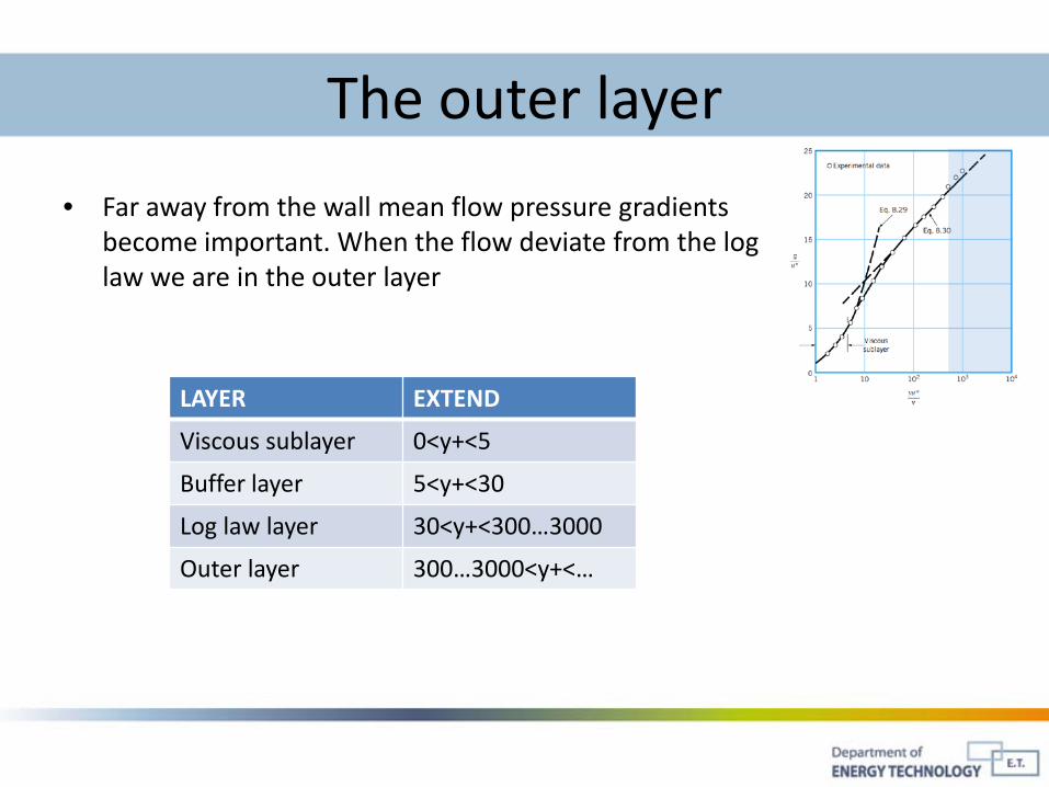
The outer layer

• Far away from the wall mean flow pressure gradients become important. When the flow deviate from the log law we are in the outer layer

LAYER EXTEND

Viscous sublayer 0<y+<5

Buffer layer 5<y+<30

Log law layer 30<y+<300…3000

Outer layer 300…3000<y+<…

Some measurement of the turbulent b.layer

• Universal?

Flow over a golf ball

Flow over a golf ball

• Boundary layer separation

Flow over a golf ball

• Tripping the boundary layer

Excercises