6 Interpolation and Approximation

6.0 Introduction

In this chapter we will discuss the problem of fitting data given in the form of dis-crete points (e.g., physical measurements, output from a differential equations solver,design points for CAD, etc.) with an appropriate function s taken from some (finite-dimensional) function space S of our choice. Throughout most of the chapter the datawill be univariate, i.e., of the form (xi, yi), i = 0, . . . , n, where the xi ∈ IR are referredto as data sites (or nodes), and the yi ∈ IR as values (or ordinates). Later on we willalso consider multivariate data where xi ∈ IRd, d > 1.

The data can be fitted either by interpolation, i.e., by satisfying

s(xi) = yi, i = 0, . . . , n, (1)

or by approximation, i.e., by satisfying

‖s− y‖ < ε,

where s and y have to be considered as vectors of function or data values, and ‖ · ‖ issome discrete norm on IRn+1.

We will focus our attention on interpolation as well as on least squares approxima-tion.

If b0, . . . , bm is some basis of the function space S, then we can express s as alinear combination in the form

s(x) =m∑

j=0

ajbj(x).

The interpolation conditions (1) then lead to

m∑j=0

ajbj(xi) = yi, i = 0, . . . , n.

This represents a linear system for the expansion coefficients aj of the form

Ba = y,

where the n ×m system matrix B has entries bj(xi). We are especially interested inthose function spaces and bases for which the case m = n yields a unique solution.

Remark: Note that for least squares approximation we will want m n. For certainsituations, e.g., when we wish to satisfy certain additional shape constraints (such asmonotonicity or convexity), we will want to choose m > n, and use the non-uniquenessof the resulting system to satisfy these additional constraints.

Function spaces studied below include polynomials, piecewise polynomials, trigono-metric polynomials, and radial basis functions.

1

6.1 Polynomial Interpolation

We will begin by studying polynomials. There are several motivating factors for doingthis:

• Everyone is familiar with polynomials.

• Polynomials can be easily and efficiently evaluated using Horner’s algorithm.

• We may have heard of the Weierstrass Approximation Theorem which states thatany continuous function can be approximated arbitrarily closely by a polynomial(of sufficiently high degree).

• A lot is known about polynomial interpolation, and serves as starting point forother methods.

Formally, we are interested in solving the following

Problem: Given data (xi, yi), i = 0, . . . , n, find a polynomial p of minimal degreewhich matches the data in the sense of (1), i.e., for which

p(xi) = yi, i = 0, . . . , n.

Remark: We illustrate this problem with some numerical examples in the Maple work-sheet 578 PolynomialInterpolation.mws.

The numerical experiments suggest that n + 1 data points can be interpolated bya polynomial of degree n. Indeed,

Theorem 6.1 Let n + 1 distinct real numbers x0, x1, . . . , xn and associated valuesy0, y1, . . . , yn be given. Then there exists a unique polynomial pn of degree at mostn such that

pn(xi) = yi, i = 0, 1, . . . , n.

Proof: Assumepn(x) = a0 + a1x + a2x

2 + . . . + anxn.

Then the interpolation conditions (1) lead to the linear system Ba = y with

B =

1 x0 x2

0 . . . xn0

1 x1 x21 . . . xn

1

1 x2 x22 . . . xn

2...

......

......

1 xn x2n . . . xn

n

, a =

a0

a1

a2...

an

and y =

y0

y1

y2

. . .yn

.

For general data y this is a nonhomogeneous system, and we know that such a systemhas a unique solution if and only if the associated homogeneous system has only thetrivial solution. This, however, implies

pn(xi) = 0, i = 0, 1, . . . , n.

2

Thus, pn has n + 1 zeros. Now, the Fundamental Theorem of Algebra states that anynontrivial polynomial of degree n has n (possibly complex) zeros. Therefore pn must bethe zero polynomial, i.e., the homogeneous linear system has only the trivial solutiona0 = a1 = . . . = an = 0, and by the above comment the general nonhomogeneousproblem has a unique solution. ♠

Remark: The matrix B in the proof of Theorem 6.1 is referred to as a Vandermondematrix.

Next, we illustrate how such a (low-degree) interpolating polynomial can be deter-mined. Let’s assume we have the following data:

x 0 1 3y 1 0 4

.

Now, since we want a square linear system, we pick the dimension of the approx-imation space to be m = 3, i.e., we use quadratic polynomials. As basis we takethe monomials b0(x) = 1, b1(x) = x, and b2(x) = x2. Therefore, the interpolatingpolynomial will be of the form

p(x) = a0 + a1x + a2x2.

In order to determine the coefficients a0, a1, and a2 we enforce the interpolation con-ditions (1), i.e., p(xi) = yi, i = 0, 1, 2. This leads to the linear system

(p(0) =) a0 = 1(p(1) =) a0 + a1 + a2 = 0(p(3) =) a0 + 3a1 + 9a2 = 4

whose solution is easily verified to be a0 = 1, a1 = −2, and a2 = 1. Thus,

p(x) = 1− 2x + x2.

Of course, this polynomial can also be written as

p(x) = (1− x)2.

So, had we chosen the basis of shifted monomials b0(x) = 1, b1(x) = 1 − x, andb2(x) = (1 − x)2, then the coefficients (for an expansion with respect to this basis)would have come out to be a0 = 0, a1 = 0, and a2 = 1.

In general, use of the monomial basis leads to a Vandermonde system as listed inthe proof above. This is a classical example of an ill-conditioned system, and thusshould be avoided. We will look at other bases later.

We now provide a second (constructive) proof of Theorem 6.1.

Constructive Proof: First we establish uniqueness. To this end we assume that pn

and qn both are n-th degree interpolating polynomials. Then

rn(x) = pn(x)− qn(x)

3

is also an n-th degree polynomial. Moreover, by the Fundamental Theorem of Algebrarn has n zeros (or is the zero polynomial). However, by the nature of pn and qn wehave

rn(xi) = pn(xi)− qn(xi) = yi − yi = 0, i = 0, 1, . . . , n.

Thus, rn has n + 1 zeros, and therefore must be identically equal to zero. This ensuresuniqueness.

Existence is constructed by induction. For n = 0 we take p0 ≡ y0. Obviously, thedegree of p0 is less than or equal to 0, and also p0(x0) = y0.

Now we assume pk−1 to be the unique polynomial of degree at most k − 1 thatinterpolates the data (xi, yi), i = 0, 1, . . . , k − 1. We will construct pk (of degree k)such that

pk(xi) = yi, i = 0, 1, . . . , k.

We letpk(x) = pk−1(x) + ck(x− x0)(x− x1) . . . (x− xk−1)

with ck yet to be determined. By construction, pk is a polynomial of degree k whichinterpolates the data (xi, yi), i = 0, 1, . . . , k − 1.

We now determine ck so that we also have pk(xk) = yk. Thus,

(pk(xk) =) pk−1(xk) + ck(xk − x0)(xk − x1) . . . (xk − xk−1) = yk

orck =

yk − pk−1(xk)(xk − x0)(xk − x1) . . . (xk − xk−1)

.

This is well defined since the denominator is nonzero due to the fact that we assumedistinct data sites. ♠

The construction used in this alternate proof provides the starting point for theNewton form of the interpolating polynomial.

Newton Form

From the proof we have

pk(x) = pk−1(x) + ck(x− x0)(x− x1) . . . (x− xk−1)= pk−2(x) + ck−1(x− x0)(x− x1) . . . (x− xk−2) + ck(x− x0)(x− x1) . . . (x− xk−1)...= c0 + c1(x− x0) + c2(x− x0)(x− x1) + . . . + ck(x− x0)(x− x1) . . . (x− xk−1).

Thus, the Newton form of the interpolating polynomial is given by

pn(x) =n∑

j=0

cj

j−1∏i=0

(x− xi). (2)

This notation implies that the empty product (when j − 1 < 0) is equal to 1.The earlier proof also provides a formula for the coefficients in the Newton form:

cj =yj − pj−1(xj)

(xj − x0)(xj − x1) . . . (xj − xj−1), p0 ≡ c0 = y0. (3)

4

So the Newton coefficients can be computed recursively. This leads to a first algorithmfor the solution of the interpolation problem.

Algorithm

Input n, x0, x1, . . . , xn, y0, y1, . . . , yn

c0 = y0

for k from 1 to n do

d = xk − xk−1

u = ck−1

for i from k − 2 by −1 to 0 do % build pk−1

u = u(xk − xi) + ci % Hornerd = d(xk − xi) % accumulate denominator

end

ck = yk−ud

end

Output c0, c1, . . . , cn

Remark: A more detailed derivation of this algorithm is provided in the textbookon page 310. However, the standard, more efficient, algorithm for computing thecoefficients of the Newton form (which is based on the use of divided differences) ispresented in the next section.

Example: We now compute the Newton form of the polynomial interpolating the data

x 0 1 3y 1 0 4

.

According to (2) and (3) we have

p2(x) =2∑

j=0

cj

j−1∏i=0

(x− xi) = c0 + c1(x− x0) + c2(x− x0)(x− x1)

with

c0 = y0 = 1, and cj =yj − pj−1(xj)

(xj − x0)(xj − x1) . . . (xj − xj−1), j = 1, 2.

Thus, we are representing the space of quadratic polynomials with the basis b0(x) = 1,b1(x) = x− x0 = x, and b2(x) = (x− x0)(x− x1) = x(x− 1).

We now determine the two remaining coefficients. First,

c1 =y1 − p0(x1)

x1 − x0=

y1 − y0

x1 − x0=

0− 11− 0

= −1.

5

This gives usp1(x) = c0 + c1(x− x0) = 1− x.

Next,

c2 =y2 − p1(x2)

(x2 − x0)(x2 − x1)=

4− (1− x2)3 · 2

= 1,

and sop2(x) = p1(x) + c2(x− x0)(x− x1) = 1− x + x(x− 1).

Lagrange Form

A third representation (after the monomial and Newton forms) of the same (unique)interpolating polynomial is of the general form

pn(x) =n∑

j=0

yj`j(x). (4)

Note that the coefficients here are the data values, and the polynomial basis functions`j are so-called cardinal (or Lagrange) functions. We want these functions to depend onthe data sites x0, x1, . . . , xn, but not the data values y0, y1, . . . , yn. In order to satisfythe interpolation conditions (1) we require

pn(xi) =n∑

j=0

yj`j(xi) = yi, i = 0, 1, . . . , n.

Clearly, this is ensured if`j(xi) = δij , (5)

which is called a cardinality (or Lagrange) condition.How do we determine the Lagrange functions `j?We want them to be polynomials of degree n and satisfy the cardinality conditions

(5). Let’s fix j, and assume

`j(x) = c(x− x0)(x− x1) . . . (x− xj−1)(x− xj+1) . . . (x− xn)

= cn∏

i=0i6=j

(x− xi).

Clearly, `j(xi) = 0 for j 6= i. Also, `j depends only on the data sites and is a polynomialof degree n. The last requirement is `j(xj) = 1. Thus,

1 = cn∏

i=0i6=j

(xj − xi)

orc =

1n∏

i=0i6=j

(xj − xi).

6

Again, the denominator is nonzero since the data sites are assumed to be distinct.Therefore, the Lagrange functions are given by

`j(x) =n∏

i=0i6=j

x− xi

xj − xi, j = 0, 1, . . . , n,

and the Lagrange form of the interpolating polynomial is

pn(x) =n∑

j=0

yj

n∏i=0i6=j

x− xi

xj − xi. (6)

Remarks:

1. We mentioned above that the monomial basis results in an interpolation matrix(a Vandermonde matrix) that is notoriously ill-conditioned. However, an advan-tage of the monomial basis representation is the fact that the interpolant can beevaluated efficiently using Horner’s method.

2. The interpolation matrix for the Lagrange form is the identity matrix and thecoefficients in the basis expansion are given by the data values. This makes theLagrange form ideal for situations in which many experiments with the same datasites, but different data values need to be performed. However, evaluation (aswell as differentiation or integration) is more expensive.

3. A major advantage of the Newton form is its efficiency in the case of adaptiveinterpolation, i.e., when an existing interpolant needs to be refined by addingmore data. Due to the recursive nature, the new interpolant can be determinedby updating the existing one (as we did in the example above). If we were toform the interpolation matrix for the Newton form we would get a triangularmatrix. Therefore, for the Newton form we have a balance between stability ofcomputation and ease of evaluation.

Example: Returning to our earlier example, we now compute the Lagrange form ofthe polynomial interpolating the data

x 0 1 3y 1 0 4

.

According to (4) we have

p2(x) =2∑

j=0

yj`j(x) = `0(x) + 4`2(x),

where (see (6))

`j(x) =2∏

i=0i6=j

x− xi

xj − xi.

7

Thus,

`0(x) =(x− x1)(x− x2)

(x0 − x1)(x0 − x2)=

(x− 1)(x− 3)(−1)(−3)

=13(x− 1)(x− 3),

and`2(x) =

(x− x0)(x− x1)(x2 − x0)(x2 − x1)

=x(x− 1)

(3− 0)(3− 1)=

16x(x− 1).

This gives us

p2(x) =13(x− 1)(x− 3) +

23x(x− 1).

Note that here we have represented the space of quadratic polynomials with the (cardi-nal) basis b0(x) = 1

3(x− 1)(x− 3), b2(x) = 16x(x− 1), and b1(x) = `1(x) = −1

2x(x− 3)(which we did not need to compute here).

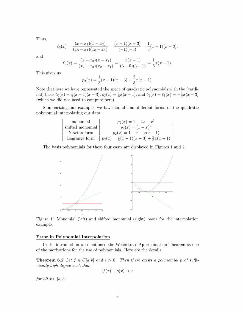
Summarizing our example, we have found four different forms of the quadraticpolynomial interpolating our data:

monomial p2(x) = 1− 2x + x2

shifted monomial p2(x) = (1− x)2

Newton form p2(x) = 1− x + x(x− 1)Lagrange form p2(x) = 1

3(x− 1)(x− 3) + 23x(x− 1)

The basis polynomials for these four cases are displayed in Figures 1 and 2.

0

2

4

6

8

0.5 1 1.5 2 2.5 3

x

–2

–1

0

1

2

3

4

0.5 1 1.5 2 2.5 3

x

Figure 1: Monomial (left) and shifted monomial (right) bases for the interpolationexample.

Error in Polynomial Interpolation

In the introduction we mentioned the Weierstrass Approximation Theorem as oneof the motivations for the use of polynomials. Here are the details.

Theorem 6.2 Let f ∈ C[a, b] and ε > 0. Then there exists a polynomial p of suffi-ciently high degree such that

|f(x)− p(x)| < ε

for all x ∈ [a, b].

8

0

1

2

3

4

5

6

0.5 1 1.5 2 2.5 3

x

–0.2

0

0.2

0.4

0.6

0.8

1

0.5 1 1.5 2 2.5 3

x

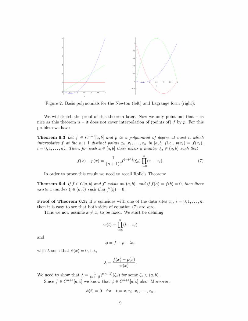
Figure 2: Basis polynomials for the Newton (left) and Lagrange form (right).

We will sketch the proof of this theorem later. Now we only point out that – asnice as this theorem is – it does not cover interpolation of (points of) f by p. For thisproblem we have

Theorem 6.3 Let f ∈ Cn+1[a, b] and p be a polynomial of degree at most n whichinterpolates f at the n + 1 distinct points x0, x1, . . . , xn in [a, b] (i.e., p(xi) = f(xi),i = 0, 1, . . . , n). Then, for each x ∈ [a, b] there exists a number ξx ∈ (a, b) such that

f(x)− p(x) =1

(n + 1)!f (n+1)(ξx)

n∏i=0

(x− xi). (7)

In order to prove this result we need to recall Rolle’s Theorem:

Theorem 6.4 If f ∈ C[a, b] and f ′ exists on (a, b), and if f(a) = f(b) = 0, then thereexists a number ξ ∈ (a, b) such that f ′(ξ) = 0.

Proof of Theorem 6.3: If x coincides with one of the data sites xi, i = 0, 1, . . . , n,then it is easy to see that both sides of equation (7) are zero.

Thus we now assume x 6= xi to be fixed. We start be defining

w(t) =n∏

i=0

(t− xi)

andφ = f − p− λw

with λ such that φ(x) = 0, i.e.,

λ =f(x)− p(x)

w(x).

We need to show that λ = 1(n+1)!f

(n+1)(ξx) for some ξx ∈ (a, b).Since f ∈ Cn+1[a, b] we know that φ ∈ Cn+1[a, b] also. Moreover,

φ(t) = 0 for t = x, x0, x1, . . . , xn.

9

The first of these equations holds by the definition of λ, the remainder by the definitionof w and the fact that p interpolates f at these points.

Now we apply Rolle’s Theorem to φ on each of the n + 1 subintervals generated bythe n + 2 points x, x0, x1, . . . , xn. Thus, φ′ has (at least) n + 1 distinct zeros in (a, b).

Next, by Rolle’s Theorem (applied to φ′ on n subintervals) we know that φ′′ has(at least) n zeros in (a, b).

Continuing this argument we deduce that φ(n+1) has (at least) one zero, ξx, in (a, b).On the other hand, since

φ(t) = f(t)− p(t)− λw(t)

we haveφ(n+1)(t) = f (n+1)(t)− p(n+1)(t)− λw(n+1)(t).

However, p is a polynomial of degree at most n, so p(n+1) ≡ 0. For w we have

w(n+1)(t) =dn+1

dtn+1

n∏i=0

(t− xi) = (n + 1)!.

Therefore,φ(n+1)(t) = f (n+1)(t)− λ(n + 1)!.

Combining this with the information about the zero of φ(n+1) we have

0 = φ(n+1)(ξx) = f (n+1)(ξx)− λ(n + 1)!

= f (n+1)(ξx)− f(x)− p(x)w(x)

(n + 1)!

orf(x)− p(x) = f (n+1)(ξx)

w(x)(n + 1)!

.

♠

Remarks:

1. The error formula (7) in Theorem 6.3 looks almost like the error formula forTaylor polynomials:

f(x)− Tn(x) =f (n+1)(ξx)(n + 1)!

(x− x0)n+1.

The difference lies in the fact that for Taylor polynomials the information is con-centrated at one point x0, whereas for interpolation the information is obtainedat the points x0, x1, . . . , xn.

2. The error formula (7) will be used later to derive (and judge the accuracy of)methods for solving differential equations as well as for numerical differentiationand integration.

10

If the data sites are equally spaced, i.e., ∆xi = xi − xi−1 = h, i = 1, 2, . . . , n, it ispossible to derive the bound

n∏i=0

|x− xi| ≤14hn+1n!

in the error formula (7). If we also assume that the derivatives of f are bounded, i.e.,|f (n+1)(x)| ≤ M for all x ∈ [a, b], then we get

|f(x)− p(x)| ≤ M

4(n + 1)hn+1.

Thus, the error for interpolation with degree-n polynomials is O(hn+1). We illustratethis formula for a fixed-degree polynomial in the Maple worksheet578 PolynomialInterpolationError.mws.

Formula (7) tells us that the interpolation error depends on the function we’reinterpolating as well as the data sites (interpolation nodes) we use. If we are interestedin minimizing the interpolation error, then we need to choose the data sites xi, i =0, 1, . . . , n, such that

w(t) =n∏

i=0

(t− xi)

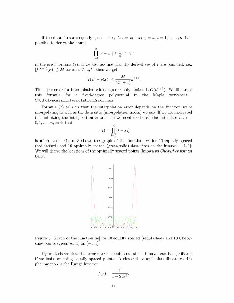
is minimized. Figure 3 shows the graph of the function |w| for 10 equally spaced(red,dashed) and 10 optimally spaced (green,solid) data sites on the interval [−1, 1].We will derive the locations of the optimally spaced points (known as Chebyshev points)below.

0

0.002

0.004

0.006

0.008

0.01

0.012

–1 –0.8 –0.6 –0.4 –0.2 0.2 0.4 0.6 0.8 1

x

Figure 3: Graph of the function |w| for 10 equally spaced (red,dashed) and 10 Cheby-shev points (green,solid) on [−1, 1].

Figure 3 shows that the error near the endpoints of the interval can be significantif we insist on using equally spaced points. A classical example that illustrates thisphenomenon is the Runge function

f(x) =1

1 + 25x2.

11

We present this example in the Maple worksheet 578 Runge.mws.In order to discuss Chebyshev points we need to introduce a certain family of

orthogonal polynomials called Chebyshev polynomials.

Chebyshev Polynomials

The Chebyshev polynomials (of the first kind) can be defined recursively. We have

T0(x) = 1, T1(x) = x,

andTn+1(x) = 2xTn(x)− Tn−1(x), n ≥ 1. (8)

An explicit formula for the n-th degree Chebyshev polynomial is

Tn(x) = cos(n arccos x), x ∈ [−1, 1], n = 0, 1, 2, . . . . (9)

We can verify this explicit formula by using the trigonometric identity

cos(A + B) = cos A cos B − sin A sinB.

This identity gives rise to the following two formulas:

cos(n + 1)θ = cos nθ cos θ − sinnθ sin θcos(n− 1)θ = cos nθ cos θ + sin nθ sin θ.

Addition of these two formulas yields

cos(n + 1)θ + cos(n− 1)θ = 2 cos nθ cos θ. (10)

Now, if we let x = cos θ (or θ = arccos x) then (10) becomes

cos [(n + 1) arccos x] + cos [(n− 1) arccos x] = 2 cos (n arccos x) cos (arccos x)

orcos [(n + 1) arccos x] = 2x cos (n arccos x)− cos [(n− 1) arccos x] ,

which is of the same form as the recursion (8) for the Chebyshev polynomials providedwe identify Tn with the explicit formula (9).

Some properties of Chebyshev polynomials are

1. |Tn(x)| ≤ 1, x ∈ [−1, 1].

2. Tn

(cos

iπ

n

)= (−1)i, i = 0, 1, . . . , n. These are the extrema of Tn.

3. Tn

(cos

2i− 12n

π

)= 0, i = 1, . . . , n. This gives the zeros of Tn.

4. The leading coefficient of Tn, n = 1, 2, . . ., is 2n−1, i.e.,

Tn(x) = 2n−1xn + lower order terms.

12

Items 1–3 follow immediately from (9). Item 4 is clear from the recursion formula(8). Therefore, 21−nTn is a monic polynomial, i.e., its leading coefficient is 1. We willneed the following property of monic polynomials below.

Theorem 6.5 For any monic polynomial p of degree n on [−1, 1] we have

‖p‖∞ = max−1≤x≤1

|p(x)| ≥ 21−n.

Proof: Textbook page 317. ♠

We are now ready to return to the formula for the interpolation error. From (7) weget on [−1, 1]

‖f − p‖∞ = max−1≤x≤1

|f(x)− p(x)|

≤ 1(n + 1)!

max−1≤x≤1

∣∣∣f (n+1)(x)∣∣∣ max−1≤x≤1

∣∣∣ n∏i=0

(x− xi)︸ ︷︷ ︸=w(x)

∣∣∣.

We note that w is a monic polynomial of degree n + 1, and therefore

max−1≤x≤1

|w(x)| ≥ 2−n.

From above we know that 2−nTn+1 is also a monic polynomial of degree n + 1 with

extrema Tn+1

(cos

iπ

n + 1

)=

(−1)i

2n, i = 0, 1, . . . , n + 1. By Theorem 6.5 the minimal

value of max−1≤x≤1

|w(x)| is 2−n. We just observed that this value is attained for Tn+1.

Thus, the zeros xi of the optimal w should coincide with the zeros of Tn+1, or

xi = cos(

2i + 12n + 2

π

), i = 0, 1, . . . , n. (11)

These are the Chebyshev points used in Figure 3 and in the Maple worksheet 578 Runge.mws.

If the data sites are taken to be the Chebyshev points on [−1, 1], then the interpo-lation error (7) becomes

|f(x)− p(x)| ≤ 12n(n + 1)!

max−1≤t≤1

∣∣∣f (n+1)(t)∣∣∣ , |x| ≤ 1.

Remark: The Chebyshev points (11) are for interpolation on [−1, 1]. If a differentinterval is used, the Chebyshev points need to be transformed accordingly.

We just observed that the Chebyshev nodes are ”optimal” interpolation points inthe sense that for any given f and fixed degree n of the interpolating polynomial, ifwe are free to choose the data sites, then the Chebyshev points will yield the mostaccurate approximation (measured in the maximum norm).

For equally spaced interpolation points, our numerical examples in the Maple work-sheets 578 PolynomialInterpolation.mws and 578 Runge.mws have shown that, con-trary to our intuition, the interpolation error (measured in the maximum norm) does

13

not tend to zero as we increase the number of interpolation points (or polynomialdegree).

The situation is even worse. There is also the following more general result provedby Faber in 1914.

Theorem 6.6 For any fixed system of interpolation nodes a ≤ x(n)0 < x

(n)1 < . . . <

x(n)n ≤ b there exists a function f ∈ C[a, b] such that the interpolating polynomial pn

does not uniformly converge to f , i.e.,

‖f − pn‖∞ 6→ 0, n →∞.

This, however, needs to be contrasted with the positive result (very much in thespirit of the Weierstrass Approximation Theorem) for the situation in which we arefree to choose the location of the interpolation points.

Theorem 6.7 Let f ∈ C[a, b]. Then there exists a system of interpolation nodes suchthat

‖f − pn‖∞ → 0, n →∞.

Proof: Uses the Weierstrass Approximation Theorem as well as the Chebyshev Alter-nation Theorem. ♠

Finally, if we insist on using the Chebyshev points as data sites, then we have thefollowing theorem due to Fejer.

Theorem 6.8 Let f ∈ C[−1, 1], and x0, x1, . . . , xn−1 be the first n Chebyshev points.Then there exists a polynomial p2n−1 of degree 2n−1 that interpolates f at x0, x1, . . . , xn−1,and for which

‖f − p2n−1‖∞ → 0, n →∞.

Remark: The polynomial p2n−1 also has zero derivatives at xi, i = 0, 1, . . . , n− 1.

We now outline the classical (constructive) proof of the Weierstrass ApproximationTheorem.

The main ingredient are the so-called Bernstein polynomials.

Definition 6.9 For any f ∈ C[0, 1]

(Bnf)(x) =n∑

k=0

f

(k

n

)(n

k

)xk(1− x)n−k, x ∈ [0, 1],

is called the n-th degree Bernstein polynomial associated with f .

Here (n

k

)=

n!k!(n− k)!

, 0 ≤ k ≤ n,

0 otherwise.The main steps of the proof of the Weierstrass Approximation Theorem (trans-

formed to the interval [0, 1]) are now

14

1. Prove the Bohman-Korovkin Theorem

Theorem 6.10 Let Ln (n ≥ 1) be a sequence of positive linear operators. If‖Lnf−f‖∞ → 0 for f(x) = 1, x, and x2, then ‖Lnf−f‖∞ → 0 for all f ∈ C[a, b].

2. Show that the Bernstein polynomials give rise to positive linear operators fromC[0, 1] to C[0, 1], i.e., show

(a) Bn is linear, i.e.,Bn(αf + βg) = αBnf + βBng,

(b) Bnf ≥ 0 provided f ≥ 0.

3. Show Bn1 = 1, Bnx = x, and Bnx2 → x2, n →∞.

Details are provided in the textbook on pages 321–323.

We illustrate the convergence behavior of the Weierstrass Approximation Theorembased on Bernstein polynomials in the Maple worksheet 578 Bezier.mws. It is generallyaccepted that the speed of convergence is too slow for practical purposes. In fact, onecan show that in order to have a maximum error smaller than 0.01 one needs at leasta degree of 1.6× 107.

Remark: The Bernstein basis polynomials (cf. Definition 6.9, and Figure 4)

Bnk (x) =

(n

k

)xk(1− x)n−k

play an important role in computer-aided geometric design (CAGD). There, so-calledBezier curves are parametric curves defined by

x(t) =n∑

k=0

bkBnk (t), t ∈ [0, 1].

Here the bk, k = 0, 1, . . . , n, are points in IR2 or IR3 referred to as control points. Thus,x can describe either a planar curve, or a curve in space. The Bezier representation ofa parametric curve has such nice properties as fast (recursive) evaluation and intuitiveshape control. 578 Bezier.mws contains examples of a 2D and 3D Bezier curve alongwith its control polygon formed by the control points bk, k = 0, . . . , n.

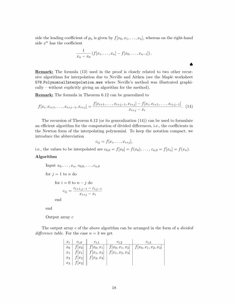
6.2 Divided Differences

Recall the Newton form of the interpolating polynomial (2)

pn(x) =n∑

j=0

cj

j−1∏k=0

(x− xk)︸ ︷︷ ︸=bj(x), (b0(x)=1)

=n∑

j=0

cjbj(x).

If we enforce the interpolation conditions

pn(xi) = f(xi), i = 0, 1, . . . , n,

15

0

0.2

0.4

0.6

0.8

1

0.2 0.4 0.6 0.8 1

x

Figure 4: Graph of the cubic Bernstein basis polynomials on [0, 1].

then we obtain a linear system of the form

Bc = f,

where Bij = bj(xi). As mentioned earlier, the matrix B is lower triangular. This isclear since

bj(xi) =j−1∏k=0

(xi − xk) = 0 if i < j.

In fact, in detail the linear system looks like

1 0 0 . . . 01 x1 − x0 0 . . . 01 x2 − x0 (x2 − x0)(x2 − x1) 0...

......

. . ....

1 xn − x0 (xn − x0)(xn − x1) . . .n−1∏k=0

(xn − xk)

c0

c1

c2...

cn

=

f(x0)f(x1)f(x2)

...f(xn)

.

We see that c0 = f(x0), and c1 depends on x0, x1, and f at those points. Similarly, cn

depends on all the points x0, x1, . . . , xn, as well as f at those points. We indicate thisdependence with the symbolic notation

cn = f [x0, x1, . . . , xn].

With this new notation the Newton form becomes

pn(x) =n∑

j=0

f [x0, x1, . . . , xj ]j−1∏k=0

(x− xk). (12)

Since the Newton form of the interpolating polynomial is constructed recursively, andsince each of the basis functions bj is a monic polynomial, we can define

16

Definition 6.11 The coefficient cn of the unique polynomial of degree n interpolatingf at the distinct points x0, x1, . . . , xn is denoted by

cn = f [x0, x1, . . . , xn],

and called the n-th order divided difference of f at x0, x1, . . . , xn.

How to Compute Divided Differences Efficiently

We begin with an example for the case n = 1, i.e., a linear polynomial. The recursiveconstruction of the Newton form suggests

p0(x) = c0 = f(x0) = f [x0]

and

p1(x) = p0(x) + c1(x− x0)= p0(x) + f [x0, x1](x− x0).

The interpolation condition at x1 suggests

p1(x1) = p0(x1)︸ ︷︷ ︸=f(x0)

+f [x0, x1](x1 − x0) = f(x1).

Solving this for the first order divided difference yields

f [x0, x1] =f(x1)− f(x0)

x1 − x0,

which explains the use of the term ”divided difference”.For the general case we have

Theorem 6.12 Let the distinct points x0, x1, . . . , xn and f be given. Then

f [x0, x1, . . . , xn−1, xn] =f [x1, . . . , xn−1, xn]− f [x0, x1, . . . , xn−1]

xn − x0.

Proof:Consider the following interpolating polynomials:

1. q (of degree n− 1) interpolating f at x1, . . . , xn,

2. pn−1 (of degree n− 1) interpolating f at x0, . . . , xn−1,

3. pn (of degree n) interpolating f at x0, . . . , xn,

Then we havepn(x) = q(x) +

x− xn

xn − x0(q(x)− pn−1(x)) . (13)

This identity was essentially proven in homework problem 6.1.9. To establish the claimof the theorem we compare the coefficients of xn on both sides of (13). For the left-hand

17

side the leading coefficient of pn is given by f [x0, x1, . . . , xn], whereas on the right-handside xn has the coefficient

1xn − x0

(f [x1, . . . , xn]− f [x0, . . . , xn−1]) .

♠

Remark: The formula (13) used in the proof is closely related to two other recur-sive algorithms for interpolation due to Neville and Aitken (see the Maple worksheet578 PolynomialInterpolation.mws where Neville’s method was illustrated graphi-cally – without explicitly giving an algorithm for the method).

Remark: The formula in Theorem 6.12 can be generalized to

f [xi, xi+1, . . . , xi+j−1, xi+j ] =f [xi+1, . . . , xi+j−1, xi+j ]− f [xi, xi+1, . . . , xi+j−1]

xi+j − xi. (14)

The recursion of Theorem 6.12 (or its generalization (14)) can be used to formulatean efficient algorithm for the computation of divided differences, i.e., the coefficients inthe Newton form of the interpolating polynomial. To keep the notation compact, weintroduce the abbreviation

cij = f [xi, . . . , xi+j ],

i.e., the values to be interpolated are c0,0 = f [x0] = f(x0), . . . , cn,0 = f [xn] = f(xn).

Algorithm

Input x0, . . . , xn, c0,0, . . . , cn,0

for j = 1 to n do

for i = 0 to n− j do

cij =ci+1,j−1 − ci,j−1

xi+j − xi

end

end

Output array c

The output array c of the above algorithm can be arranged in the form of a divideddifference table. For the case n = 3 we get

xi ci,0 ci,1 ci,2 ci,3

x0 f [x0] f [x0, x1] f [x0, x1, x2] f [x0, x1, x2, x3]x1 f [x1] f [x1, x2] f [x1, x2, x3]x2 f [x2] f [x2, x3]x3 f [x3]

18

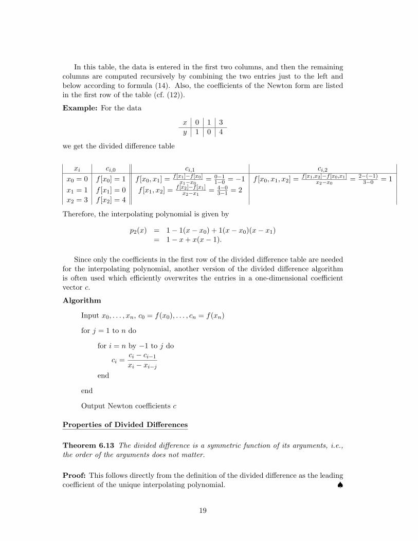
In this table, the data is entered in the first two columns, and then the remainingcolumns are computed recursively by combining the two entries just to the left andbelow according to formula (14). Also, the coefficients of the Newton form are listedin the first row of the table (cf. (12)).

Example: For the data

x 0 1 3y 1 0 4

we get the divided difference table

xi ci,0 ci,1 ci,2

x0 = 0 f [x0] = 1 f [x0, x1] = f [x1]−f [x0]x1−x0

= 0−11−0 = −1 f [x0, x1, x2] = f [x1,x2]−f [x0,x1]

x2−x0= 2−(−1)

3−0 = 1x1 = 1 f [x1] = 0 f [x1, x2] = f [x2]−f [x1]

x2−x1= 4−0

3−1 = 2x2 = 3 f [x2] = 4

Therefore, the interpolating polynomial is given by

p2(x) = 1− 1(x− x0) + 1(x− x0)(x− x1)= 1− x + x(x− 1).

Since only the coefficients in the first row of the divided difference table are neededfor the interpolating polynomial, another version of the divided difference algorithmis often used which efficiently overwrites the entries in a one-dimensional coefficientvector c.

Algorithm

Input x0, . . . , xn, c0 = f(x0), . . . , cn = f(xn)

for j = 1 to n do

for i = n by −1 to j do

ci =ci − ci−1

xi − xi−j

end

end

Output Newton coefficients c

Properties of Divided Differences

Theorem 6.13 The divided difference is a symmetric function of its arguments, i.e.,the order of the arguments does not matter.

Proof: This follows directly from the definition of the divided difference as the leadingcoefficient of the unique interpolating polynomial. ♠

19

Theorem 6.14 Let x0, x1, . . . , xn be distinct nodes, and let p be the unique polynomialinterpolating f at these nodes. If t is not a node, then

f(t)− p(t) = f [x0, x1, . . . , xn, t]n∏

i=0

(t− xi).

Proof: Let p be the degree n polynomial interpolating f at x0, x1, . . . , xn, and q thedegree n+1 interpolating polynomial to f at x0, x1, . . . , xn, t. By the recursive Newtonconstruction we have

q(x) = p(x) + f [x0, x1, . . . , xn, t]n∏

i=0

(x− xi). (15)

Now, since q(t) = f(t), the statement follows immediately by replacing x by t in (15).♠

If we compare the statement of Theorem 6.14 with that of Theorem 6.3 we get

Theorem 6.15 If f ∈ Cn[a, b] and x0, x1, . . . , xn are distinct points in [a, b], then thereexists a ξ ∈ (a, b) such that

f [x0, x1, . . . , xn] =1n!

f (n)(ξ).

Remark: Divided differences can be used to estimate derivatives. This idea is, e.g.,employed in the construction of so-called ENO (essentially non-oscillating) methods forsolving hyperbolic PDEs.

6.3 Hermite Interpolation

Now we consider the situation in which we also want to interpolate derivative informa-tion at the data sites. In order to be able to make a statement about the solvability ofthis kind of problem we will have to impose some restrictions.

To get an idea of the nature of those restrictions we begin with a few simple exam-ples.

Example 1: If the data is given by the following four pieces of information

f(0) = 1, f(1) = 0, f ′(0) = 0, f ′(1) = 0,

then we should attempt to interpolate with a polynomial of degree three, i.e.,

p3(x) = a0 + a1x + a2x2 + a3x

3.

Since we also need to match derivative information, we need the derivative of thepolynomial

p′3(x) = a1 + 2a2x + 3a3x2.

The four interpolation conditions

p3(0) = a0 = f(0) = 1

20

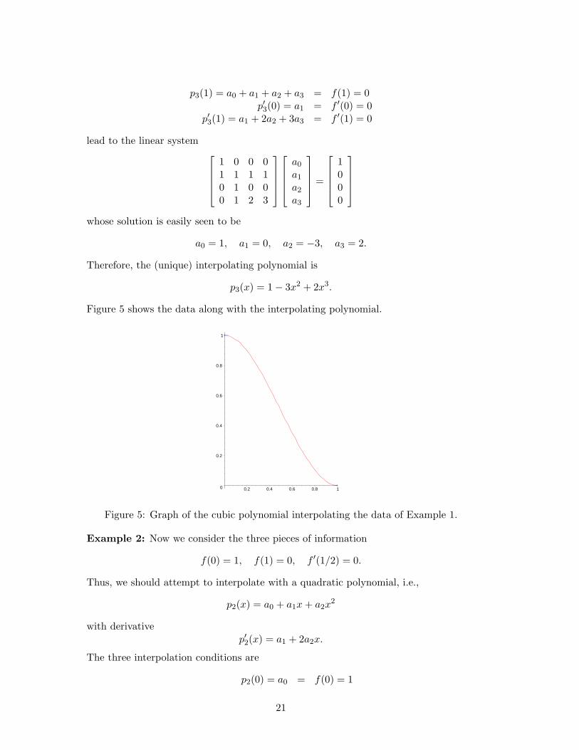
p3(1) = a0 + a1 + a2 + a3 = f(1) = 0p′3(0) = a1 = f ′(0) = 0

p′3(1) = a1 + 2a2 + 3a3 = f ′(1) = 0

lead to the linear system 1 0 0 01 1 1 10 1 0 00 1 2 3

a0

a1

a2

a3

=

1000

whose solution is easily seen to be

a0 = 1, a1 = 0, a2 = −3, a3 = 2.

Therefore, the (unique) interpolating polynomial is

p3(x) = 1− 3x2 + 2x3.

Figure 5 shows the data along with the interpolating polynomial.

0

0.2

0.4

0.6

0.8

1

0.2 0.4 0.6 0.8 1

Figure 5: Graph of the cubic polynomial interpolating the data of Example 1.

Example 2: Now we consider the three pieces of information

f(0) = 1, f(1) = 0, f ′(1/2) = 0.

Thus, we should attempt to interpolate with a quadratic polynomial, i.e.,

p2(x) = a0 + a1x + a2x2

with derivativep′2(x) = a1 + 2a2x.

The three interpolation conditions are

p2(0) = a0 = f(0) = 1

21

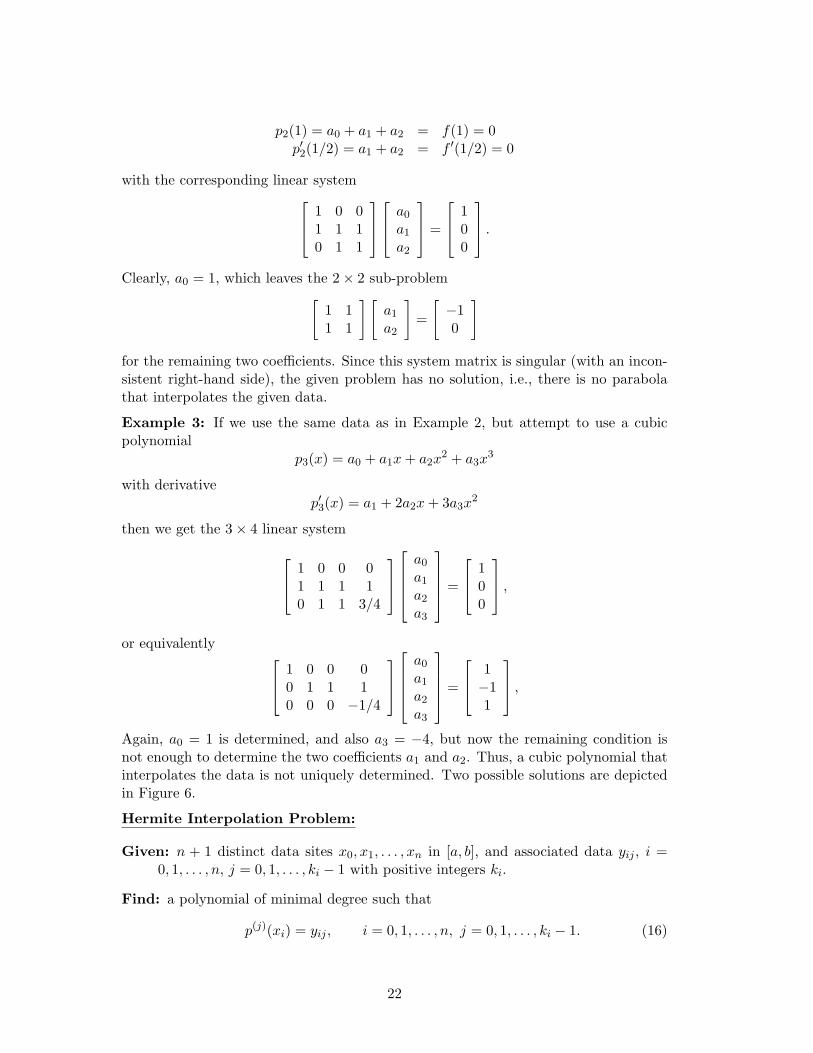
p2(1) = a0 + a1 + a2 = f(1) = 0p′2(1/2) = a1 + a2 = f ′(1/2) = 0

with the corresponding linear system 1 0 01 1 10 1 1

a0

a1

a2

=

100

.

Clearly, a0 = 1, which leaves the 2× 2 sub-problem[1 11 1

] [a1

a2

]=

[−10

]

for the remaining two coefficients. Since this system matrix is singular (with an incon-sistent right-hand side), the given problem has no solution, i.e., there is no parabolathat interpolates the given data.

Example 3: If we use the same data as in Example 2, but attempt to use a cubicpolynomial

p3(x) = a0 + a1x + a2x2 + a3x

3

with derivativep′3(x) = a1 + 2a2x + 3a3x

2

then we get the 3× 4 linear system

1 0 0 01 1 1 10 1 1 3/4

a0

a1

a2

a3

=

100

,

or equivalently 1 0 0 00 1 1 10 0 0 −1/4

a0

a1

a2

a3

=

1−11

,

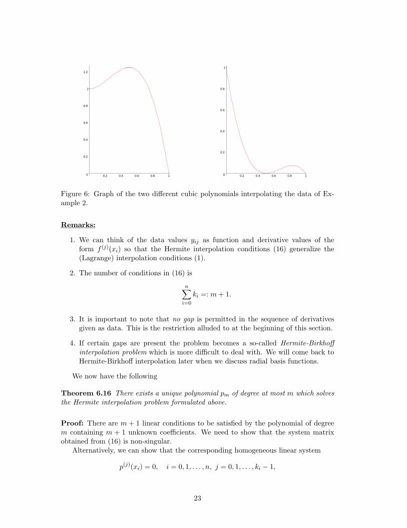
Again, a0 = 1 is determined, and also a3 = −4, but now the remaining condition isnot enough to determine the two coefficients a1 and a2. Thus, a cubic polynomial thatinterpolates the data is not uniquely determined. Two possible solutions are depictedin Figure 6.

Hermite Interpolation Problem:

Given: n + 1 distinct data sites x0, x1, . . . , xn in [a, b], and associated data yij , i =0, 1, . . . , n, j = 0, 1, . . . , ki − 1 with positive integers ki.

Find: a polynomial of minimal degree such that

p(j)(xi) = yij , i = 0, 1, . . . , n, j = 0, 1, . . . , ki − 1. (16)

22

0

0.2

0.4

0.6

0.8

1

1.2

0.2 0.4 0.6 0.8 1 0

0.2

0.4

0.6

0.8

1

0.2 0.4 0.6 0.8 1

Figure 6: Graph of the two different cubic polynomials interpolating the data of Ex-ample 2.

Remarks:

1. We can think of the data values yij as function and derivative values of theform f (j)(xi) so that the Hermite interpolation conditions (16) generalize the(Lagrange) interpolation conditions (1).

2. The number of conditions in (16) is

n∑i=0

ki =: m + 1.

3. It is important to note that no gap is permitted in the sequence of derivativesgiven as data. This is the restriction alluded to at the beginning of this section.

4. If certain gaps are present the problem becomes a so-called Hermite-Birkhoffinterpolation problem which is more difficult to deal with. We will come back toHermite-Birkhoff interpolation later when we discuss radial basis functions.

We now have the following

Theorem 6.16 There exists a unique polynomial pm of degree at most m which solvesthe Hermite interpolation problem formulated above.

Proof: There are m + 1 linear conditions to be satisfied by the polynomial of degreem containing m + 1 unknown coefficients. We need to show that the system matrixobtained from (16) is non-singular.

Alternatively, we can show that the corresponding homogeneous linear system

p(j)(xi) = 0, i = 0, 1, . . . , n, j = 0, 1, . . . , ki − 1,

23

has only the trivial solution p ≡ 0. If p and its derivatives have all the stated zeros,then it must be of the form

p(x) = c (x− x0)k0(x− x1)k1 . . . (x− xn)kn︸ ︷︷ ︸=:q(x)

, (17)

with some constant c.Now,

deg(q) =n∑

i=0

ki = m + 1,

and from (17) deg(p) = deg(q) = m + 1. However, p was assumed to be of degree m(with m + 1 unknown coefficients). The only possibility is that p ≡ 0. ♠

Newton Form:

We now need to discuss divided difference with repeated arguments. First, consider

limx→x0

f [x0, x] = limx→x0

f(x)− f(x0)x− x0

= f ′(x0).

This motivates the notationf [x0, x0] = f ′(x0).

Using the identity

f [x0, x1, . . . , xk] =1k!

f (k)(ξ), ξ ∈ (x0, xk),

listed earlier in Theorem 6.15 we are led to

f [x0, . . . , x0︸ ︷︷ ︸k+1

] =1k!

f (k)(x0). (18)

Example: Consider the data

x0 = 0x1 = 1

y00(= f(x0)) = −1,y01(= f ′(x0)) = −2,y10(= f(x1)) = 0,y11(= f ′(x1)) = 10,y12(= f ′′(x1)) = 40.

Using the divided difference notation introduced in (18) this corresponds to

f [x0] = −1,f [x0, x0] = −2,

f [x1] = 0,f [x1, x1] = 10,

f [x1, x1, x1] =402!

= 20.

24

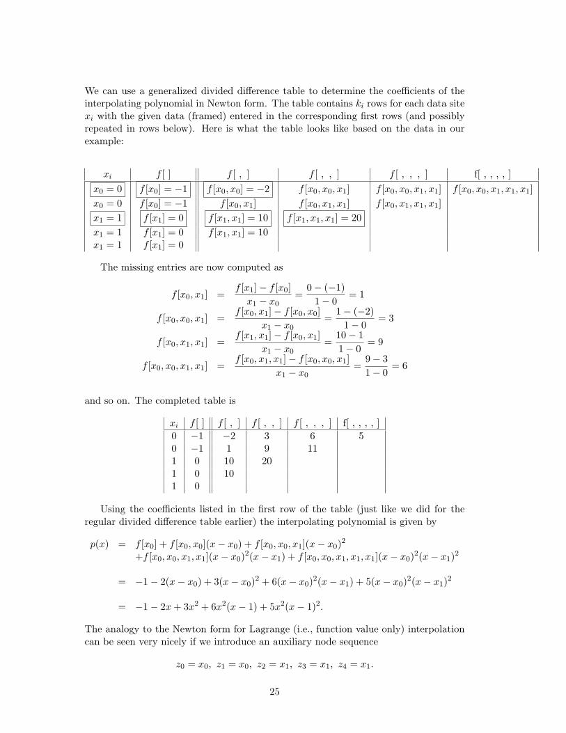
We can use a generalized divided difference table to determine the coefficients of theinterpolating polynomial in Newton form. The table contains ki rows for each data sitexi with the given data (framed) entered in the corresponding first rows (and possiblyrepeated in rows below). Here is what the table looks like based on the data in ourexample:

xi f [ ] f [ , ] f [ , , ] f [ , , , ] f[ , , , , ]x0 = 0 f [x0] = −1 f [x0, x0] = −2 f [x0, x0, x1] f [x0, x0, x1, x1] f [x0, x0, x1, x1, x1]x0 = 0 f [x0] = −1 f [x0, x1] f [x0, x1, x1] f [x0, x1, x1, x1]x1 = 1 f [x1] = 0 f [x1, x1] = 10 f [x1, x1, x1] = 20x1 = 1 f [x1] = 0 f [x1, x1] = 10x1 = 1 f [x1] = 0

The missing entries are now computed as

f [x0, x1] =f [x1]− f [x0]

x1 − x0=

0− (−1)1− 0

= 1

f [x0, x0, x1] =f [x0, x1]− f [x0, x0]

x1 − x0=

1− (−2)1− 0

= 3

f [x0, x1, x1] =f [x1, x1]− f [x0, x1]

x1 − x0=

10− 11− 0

= 9

f [x0, x0, x1, x1] =f [x0, x1, x1]− f [x0, x0, x1]

x1 − x0=

9− 31− 0

= 6

and so on. The completed table is

xi f [ ] f [ , ] f [ , , ] f [ , , , ] f[ , , , , ]0 −1 −2 3 6 50 −1 1 9 111 0 10 201 0 101 0

Using the coefficients listed in the first row of the table (just like we did for theregular divided difference table earlier) the interpolating polynomial is given by

p(x) = f [x0] + f [x0, x0](x− x0) + f [x0, x0, x1](x− x0)2

+f [x0, x0, x1, x1](x− x0)2(x− x1) + f [x0, x0, x1, x1, x1](x− x0)2(x− x1)2

= −1− 2(x− x0) + 3(x− x0)2 + 6(x− x0)2(x− x1) + 5(x− x0)2(x− x1)2

= −1− 2x + 3x2 + 6x2(x− 1) + 5x2(x− 1)2.

The analogy to the Newton form for Lagrange (i.e., function value only) interpolationcan be seen very nicely if we introduce an auxiliary node sequence

z0 = x0, z1 = x0, z2 = x1, z3 = x1, z4 = x1.

25

Then the interpolating polynomial is given by

p(x) =3∑

j=0

f [z0, . . . , zj ]j−1∏i=0

(x− zi).

Remark: The principles used in this examples can (with some notational efforts) beextended to the general Hermite interpolation problem.

The following error estimate is more general than the one provided in the textbookon page 344.

Theorem 6.17 Let x0, x1, . . . , xn be distinct data sites in [a, b], and let f ∈ Cm+1[a, b],

where m + 1 =n∑

i=0

ki. Then the unique polynomial p of degree at most m which solves

the Hermite interpolation problem satisfies

f(x)− p(x) =1

(m + 1)!f (m+1)(ξx)

n∏i=0

(x− xi)ki ,

where ξx is some point in (a, b).

Proof: Analogous to the proof of Theorem 6.3. See the textbook for the case ki = 2,i = 0, 1, . . . , n. ♠

Cardinal Hermite Interpolation

It is also possible to derive cardinal basis functions, but due to their complexitythis is rarely done. For first order Hermite interpolation, i.e., data of the form

(xi, f(xi)), (xi, f′(xi)), i = 0, 1, . . . , n,

we make the assumption that p (of degree m, since we have m+1 = 2n+2 conditions)is of the form

p(x) =n∑

j=0

f(xj)Lj(x) +n∑

j=0

f ′(xj)Mj(x).

The cardinality conditions for the basis functions are nowLj(xi) = δij

L′j(xi) = 0

Mj(xi) = 0M ′

j(xi) = δij

which can be shown to lead to

Lj(x) =(1− 2(x− xj)`′j(xj)

)`2j (x), j = 0, 1, . . . , n,

Mj(x) = (x− xj)`2j (x), j = 0, 1, . . . , n,

where

`j(x) =n∏

i=0i6=j

x− xi

xj − xi, j = 0, 1, . . . , n,

are the Lagrange basis functions of (6). Since the `j are of degree n it is easily verifiedthat Lj and Mj are of degree m = 2n + 1.

26

6.4 Spline Interpolation

One of the main disadvantages associated with polynomial interpolation were the os-cillations resulting from the use high-degree polynomials. If we want to maintain suchadvantages as simplicity, ease and speed of evaluation, as well as similar approximationproperties, we are naturally led to consider piecewise polynomial interpolation or splineinterpolation.

Definition 6.18 A spline function S of degree k is a function such that

a) S is defined on an interval [a, b],

b) S ∈ Ck−1[a, b],

c) there are points a = t0 < t1 < . . . < tn = b (called knots) such that S is apolynomial of degree at most k on each subinterval [ti, ti+1).

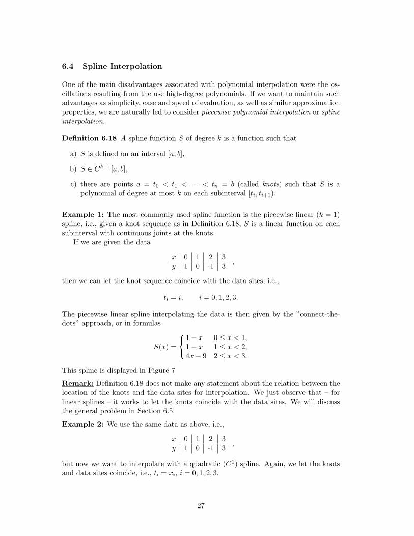
Example 1: The most commonly used spline function is the piecewise linear (k = 1)spline, i.e., given a knot sequence as in Definition 6.18, S is a linear function on eachsubinterval with continuous joints at the knots.

If we are given the data

x 0 1 2 3y 1 0 -1 3

,

then we can let the knot sequence coincide with the data sites, i.e.,

ti = i, i = 0, 1, 2, 3.

The piecewise linear spline interpolating the data is then given by the ”connect-the-dots” approach, or in formulas

S(x) =

1− x 0 ≤ x < 1,1− x 1 ≤ x < 2,4x− 9 2 ≤ x < 3.

This spline is displayed in Figure 7

Remark: Definition 6.18 does not make any statement about the relation between thelocation of the knots and the data sites for interpolation. We just observe that – forlinear splines – it works to let the knots coincide with the data sites. We will discussthe general problem in Section 6.5.

Example 2: We use the same data as above, i.e.,

x 0 1 2 3y 1 0 -1 3

,

but now we want to interpolate with a quadratic (C1) spline. Again, we let the knotsand data sites coincide, i.e., ti = xi, i = 0, 1, 2, 3.

27

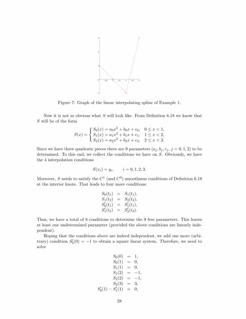
–1

0

1

2

3

0.5 1 1.5 2 2.5 3

Figure 7: Graph of the linear interpolating spline of Example 1.

Now it is not so obvious what S will look like. From Definition 6.18 we know thatS will be of the form

S(x) =

S0(x) = a0x

2 + b0x + c0, 0 ≤ x < 1,S1(x) = a1x

2 + b1x + c1, 1 ≤ x < 2,S2(x) = a2x

2 + b2x + c2, 2 ≤ x < 3.

Since we have three quadratic pieces there are 9 parameters (aj , bj , cj , j = 0, 1, 2) to bedetermined. To this end, we collect the conditions we have on S. Obviously, we havethe 4 interpolation conditions

S(xi) = yi, i = 0, 1, 2, 3.

Moreover, S needs to satisfy the C1 (and C0) smoothness conditions of Definition 6.18at the interior knots. That leads to four more conditions:

S0(t1) = S1(t1),S1(t2) = S2(t2),S′0(t1) = S′1(t1),S′1(t2) = S′2(t2).

Thus, we have a total of 8 conditions to determine the 9 free parameters. This leavesat least one undetermined parameter (provided the above conditions are linearly inde-pendent).

Hoping that the conditions above are indeed independent, we add one more (arbi-trary) condition S′0(0) = −1 to obtain a square linear system. Therefore, we need tosolve

S0(0) = 1,S0(1) = 0,S1(1) = 0,S1(2) = −1,S2(2) = −1,S2(3) = 3,

S′0(1)− S′1(1) = 0,

28

S′1(2)− S′2(2) = 0,S′0(0) = −1.

Note that we have implemented the C0 conditions at the two interior knots by statingthe interpolation conditions for both adjoining pieces. In matrix form, the resultinglinear system is

0 0 1 0 0 0 0 0 01 1 1 0 0 0 0 0 00 0 0 1 1 1 0 0 00 0 0 4 2 1 0 0 00 0 0 0 0 0 4 2 10 0 0 0 0 0 9 3 12 1 0 −2 −1 0 0 0 00 0 0 4 1 0 −4 −1 00 1 0 0 0 0 0 0 0

a0

b0

c0

a1

b1

c1

a2

b2

c2

=

100−1−1300−1

.

The solution of this linear system is given by

a0 = 0, b0 = −1, c0 = 1,a1 = 0, b1 = −1, c1 = 1,

a2 = 5, b2 = −21, c2 = 21,

or

S(x) =

1− x, 0 ≤ x < 1,1− x, 1 ≤ x < 2,5x2 − 21x + 21, 2 ≤ x < 3.

This example is illustrated in the Maple worksheet 578 SplineInterpolation.mwsand a plot of the quadratic spline computed in Example 2 is also provided in Figure 8.

–1

0

1

2

3

0.5 1 1.5 2 2.5 3

x

Figure 8: Graph of the quadratic interpolating spline of Example 2.

Remark: In order to efficiently evaluate a piecewise defined spline S at some pointx ∈ [t0, tn] one needs to be able to identify which polynomial piece to evaluate, i.e.,determine in which subinterval [ti, ti+1) the evaluation point x lies. An algorithm (forlinear splines) is given in the textbook on page 350.

29

Cubic Splines

Another very popular spline is the (C2) cubic spline. Assume we are given n + 1pieces of data (xi, yi), i = 0, 1, . . . , n to interpolate. Again, we let the knot sequenceti coincide with the data sites. According to Definition 6.18 the spline S will consistof n cubic polynomial pieces with a total of 4n parameters.

The conditions prescribed in Definition 6.18 are

n + 1 interpolation conditions,

n− 1 C0 continuity conditions at interior knots,

n− 1 C1 continuity conditions at interior knots,

n− 1 C2 continuity conditions at interior knots,

for a total of 4n− 2 conditions. Assuming linear independence of these conditions, wewill be able to impose two additional conditions on S.

There are many possible ways of doing this. We will discuss:

1. S′′(t0) = S′′(tn) = 0, (so-called natural end conditions).

2. Other boundary conditions, such as

S′(t0) = f ′(t0), S′(tn) = f ′(tn)

which lead to complete splines, or

S′′(t0) = f ′′(t0), S′′(tn) = f ′′(tn).

In either case, f ′ or f ′′ needs to be provided (or estimated) as additional data.

3. The so-called ”not-a-knot” condition.

Cubic Natural Spline Interpolation

To simplify the notation we introduce the abbreviation

zi = S′′(ti), i = 0, 1, . . . , n,

for the value of the second derivative at the knots. We point out that these values arenot given as data, but are parameters to be determined.

Since S is cubic S′′ will be linear. If we write this linear polynomial on the subin-terval [ti, ti+1) in its Lagrange form we have

S′′i (x) = ziti+1 − x

ti+1 − ti+ zi+1

x− titi+1 − ti

.

With another abbreviation hi = ti+1 − ti this becomes

S′′i (x) =zi

hi(ti+1 − x) +

zi+1

hi(x− ti). (19)

30

Remark: By assigning the value zi to both pieces joining together at ti we will auto-matically enforce continuity of the second derivative of S.

Now, we obtain a representation for the piece Si by integrating (19) twice:

Si(x) =zi

6hi(ti+1 − x)3 +

zi+1

6hi(x− ti)3 + C(x− ti) + D(ti+1 − x). (20)

The interpolation conditions (for the piece Si)

Si(ti) = yi, Si(ti+1) = yi+1

yield a 2× 2 linear system for the constants C and D. This leads to

Si(x) =zi

6hi(ti+1−x)3+

zi+1

6hi(x−ti)3+

(yi+1

hi− zi+1hi

6

)(x−ti)+

(yi

hi− zihi

6

)(ti+1−x).

(21)(Note that it is easily verified that (21) satisfies the interpolation conditions.)

Once we have determined the unknowns zi each piece of the spline S can be evalu-ated via (21). We have not yet employed the C1 continuity conditions at the interiorknots, i.e.,

S′i−1(ti) = S′i(ti), i = 1, 2, . . . , n− 1. (22)

Thus, we have n − 1 additional conditions. Since there are n + 1 unknowns zi, i =0, 1, . . . , n, we fix the second derivative at the endpoints to be zero, i.e.,

z0 = zn = 0.

These are the so-called natural end conditions. Differentiation of (21) leads to

S′i(x) = − zi

2hi(ti+1 − x)2 +

zi+1

2hi(x− ti)2 +

(yi+1

hi− zi+1hi

6

)−(

yi

hi− zihi

6

).

Using this expression in (22) results in

zi−1hi−1 +2(hi−1 +hi)zi +zi+1hi =6hi

(yi+1−yi)−6

hi−1(yi−yi−1), i = 1, 2, . . . , n−1.

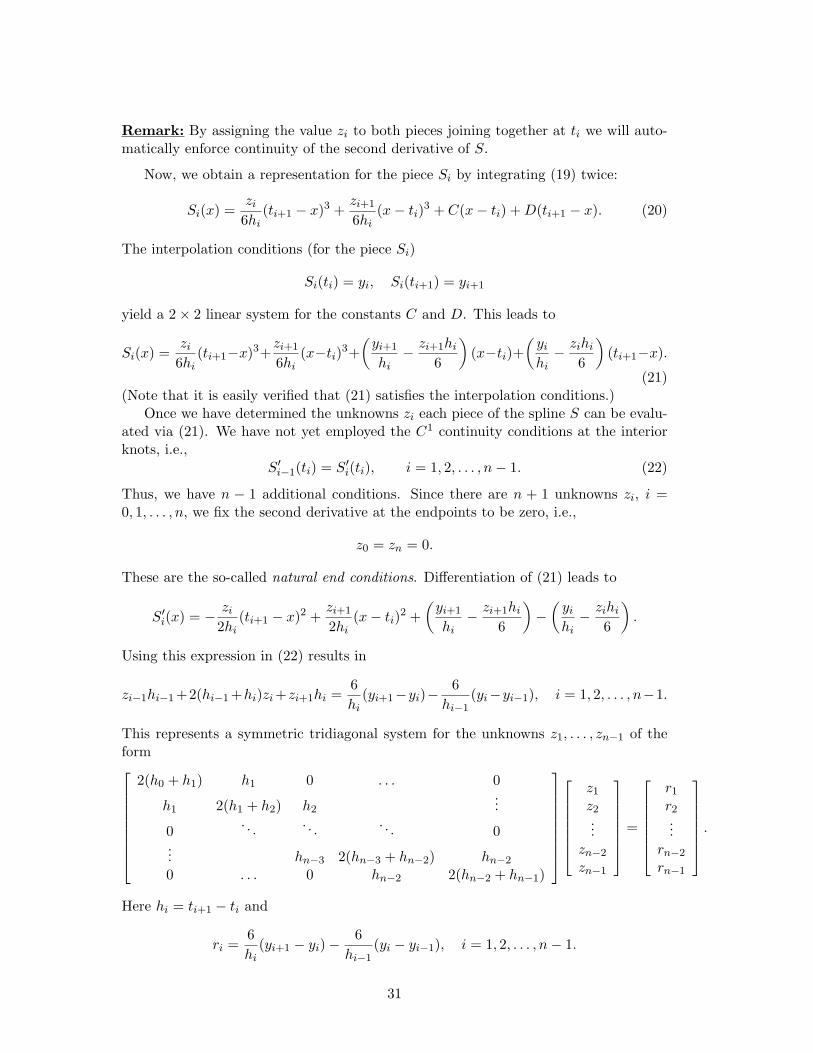
This represents a symmetric tridiagonal system for the unknowns z1, . . . , zn−1 of theform

2(h0 + h1) h1 0 . . . 0

h1 2(h1 + h2) h2...

0. . . . . . . . . 0

... hn−3 2(hn−3 + hn−2) hn−2

0 . . . 0 hn−2 2(hn−2 + hn−1)

z1

z2...

zn−2

zn−1

=

r1

r2...

rn−2

rn−1

.

Here hi = ti+1 − ti and

ri =6hi

(yi+1 − yi)−6

hi−1(yi − yi−1), i = 1, 2, . . . , n− 1.

31

Remark: The system matrix is even diagonally dominant since

2(hi−1 + hi) > hi−1 + hi

since all hi > 0 due to the fact that the knots ti are distinct and form an increasingsequence. Thus, a very efficient tridiagonal version of Gauss elimination without piv-oting can be employed to solve for the missing zi (see the textbook on page 353 forsuch an algorithm).

”Optimality” of Natural Splines

Among all smooth functions which interpolate a given function f at the knotst0, t1, . . . , tn, the natural spline is the smoothest, i.e.,

Theorem 6.19 Let f ∈ C2[a, b] and a = t0 < t1 < . . . < tn = b. If S is the cubicnatural spline interpolating f at ti, i = 0, 1, . . . , n, then∫ b

a

[S′′(x)

]2dx ≤

∫ b

a

[f ′′(x)

]2dx.

Remark: The integrals in Theorem 6.19 can be interpreted as bending energies of athin rod, or as ”total curvatures” (since for small defections the curvature κ ≈ f ′′).This optimality result is what gave rise to the name spline, since early ship designersused a piece of wood (called a spline) fixed at certain (interpolation) points to describethe shape of the ship’s hull.

Proof: Define an auxiliary function g = f − S. Then f = S + g and f ′′ = S′′ + g′′ or(f ′′)2 =

(S′′)2 +

(g′′)2 + 2S′′g′′.

Therefore,∫ b

a

(f ′′(x)

)2dx =

∫ b

a

(S′′(x)

)2dx +

∫ b

a

(g′′(x)

)2dx +

∫ b

a2S′′(x)g′′(x)dx.

Obviously, ∫ b

a

(g′′(x)

)2dx ≥ 0,

so that we are done is we can show that also∫ b

a2S′′(x)g′′(x)dx ≥ 0.

To this end we break the interval [a, b] into the subintervals [ti−1, ti], and get∫ b

aS′′(x)g′′(x)dx =

n∑i=1

∫ ti

ti−1

S′′(x)g′′(x)dx.

Now we can integrate by parts (with u = S′′(x), dv = g′′(x)dx) to obtain

n∑i=1

[S′′(x)g′(x)

]titi−1

−∫ ti

ti−1

S′′′(x)g′(x)dx

.

32

The first term is a telescoping sum so that

n∑i=1

[S′′(x)g′(x)

]titi−1

= S′′(tn)g′(tn)− S′′(t0)g′(t0) = 0

due to the natural end conditions of the spline S.This leaves ∫ b

aS′′(x)g′′(x)dx = −

n∑i=1

∫ ti

ti−1

S′′′(x)g′(x)dx.

However, since Si is a cubic polynomial we know that S′′′(x) ≡ ci on [ti−1, ti). Thus,∫ b

aS′′(x)g′′(x)dx = −

n∑i=1

ci

∫ ti

ti−1

g′(x)dx

= −n∑

i=1

ci [g(x)]titi−1= 0.

The last equation holds since g(ti) = f(ti)−S(ti), i = 0, 1, . . . , n, and S interpolates fat the knots ti. ♠

Remark: Cubic natural splines should not be considered the natural choice for cubicspline interpolation. This is due to the fact that one can show that the (rather arbitrary)choice of natural end conditions yields an interpolation error estimate of only O(h2),where h = max

i=1,...,n∆ti and ∆ti = ti − ti−1. This needs to be compared to the estimate

of O(h4) obtainable by cubic polynomials as well as other cubic spline methods.

Cubic Complete Spline Interpolation

The derivation of cubic complete splines is similar to that of the cubic naturalsplines. However, we impose the additional end constraints

S′(t0) = f ′(t0), S′(tn) = f ′(tn).

This requires additional data (f ′ at the endpoints), but can be shown to yields anO(h4) interpolation error estimate.

Moreover, an energy minimization theorem analogous to Theorem 6.19 also holdssince

n∑i=1

[S′′(x)g′(x)

]titi−1

= S′′(tn)g′(tn)− S′′(t0)g′(t0)

= S′′(tn)(f ′(tn)− S′(tn)

)− S′′(t0)

(f ′(t0)− S′(t0)

)= 0

by the end conditions.

Not-a-Knot Spline Interpolation

One of the most effective cubic spline interpolation methods is obtained by choosingthe knots different from the data sites. In particular, if the data is of the form

x0 x1 x2 . . . xn−1 xn

y0 y1 y2 . . . yn−1 yn,

33

then we take the n− 1 knots as

x0 x2 x3 . . . xn−2 xn

t0 t1 t2 . . . tn−3 tn−2,

i.e., the data sites x1 and xn−1 are ”not-a-knot”.The knots now define n−2 cubic polynomial pieces with a total of 4n−8 coefficients.

On the other hand, there are n + 1 interpolation conditions together with three sets of(n− 3) smoothness conditions at the interior knots. Thus, the number of conditions isequal to the number of unknown coefficients, and no additional (arbitrary) conditionsneed to be imposed to solve the interpolation problem.

One can interpret this approach as using only one cubic polynomial piece to repre-sent the first two (last two) data segments.

The cubic not-a-knot spline has an O(h4) interpolation error, and requires no ad-ditional data. More details can be found in the book ”A Practical Guide to Splines”by Carl de Boor.

Remarks:

1. If we are given also derivative information at the data sites xi, i = 0, 1, . . . , n,then we can perform piecewise cubic Hermite interpolation (see Section 6.3). Theresulting function will be C1 continuous, and one can show that the interpolationerror is O(h4). However, this function is not considered a spline function since itdoes not have the required smoothness.

2. There are also piecewise cubic interpolation methods that estimate derivativeinformation at the data sites, i.e., no derivative information is provided as data.Two such (local) methods are named after Bessel (yielding an O(h3) interpolationerror) and Akima (with an O(h2) error). Again, they are not spline functions asthey are only C1 smooth.

6.5 B-Splines

B-splines will generate local bases for the spaces of spline functions defined in theprevious section in Definition 6.18. Local bases are important for reasons of efficiency.Moreover, we will see that there are efficient recurrence relations for the coefficients ofthese basis functions.

B-splines were first introduced to approximation theory by Iso Schoenberg in 1946.The name ”B-spline”, however, was not used until 1967. On the other hand, thefunctions known as B-splines today came up as early as 1800 in work by Laplace andLobachevsky as convolutions of probability density functions.

The main books on B-splines are ”A Practical Guide to Splines” by Carl de Boor(1978) and ”Spline Functions: Basic Theory” by Larry Schumaker (1980). The develop-ment presented in our textbook (which we follow here) is not the traditional one (basedon the use of divided differences) given in the two main monographs, but rather basedon the paper ”B-splines without divided differences” by Carl de Boor and Klaus Hollig(1987). There are alternate derivations based on the idea of knot insertion (mostly for

34

CAGD purposes) by Wolfgang Boehm (1980), and on a method called ”blossoming”by Lyle Ramshaw (1987).

According to Definition 6.18 the space of piecewise polynomial spline functions isdetermined by the polynomial degree and a (bi-infinite) knot sequence

. . . < t−2 < t−1 < t0 < t1 < t2 < . . . .

In practice, the knot sequence is usually finite, and later on knots with varying multi-plicities will be allowed.

B-Splines of Degree 0

Definition 6.20 Given an interval [ti, ti+1), the B-spline of degree 0 is defined as

B0i (x) =

1 x ∈ [ti, ti+1),0 otherwise.

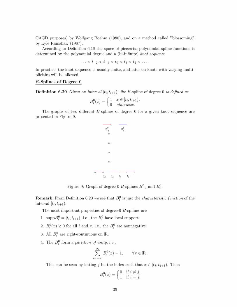
The graphs of two different B-splines of degree 0 for a given knot sequence arepresented in Figure 9.

00

B0

–2B

1t

0t

–1t

–2t

0.2

0.4

0.6

0.8

1

–2 –1 1 2 3

Figure 9: Graph of degree 0 B-splines B0−2 and B0

0 .

Remark: From Definition 6.20 we see that B0i is just the characteristic function of the

interval [ti, ti+1).

The most important properties of degree-0 B-splines are

1. suppB0i = [ti, ti+1), i.e., the B0

i have local support.

2. B0i (x) ≥ 0 for all i and x, i.e., the B0

i are nonnegative.

3. All B0i are right-continuous on IR.

4. The B0i form a partition of unity, i.e.,

∞∑i=−∞

B0i (x) = 1, ∀x ∈ IR .

This can be seen by letting j be the index such that x ∈ [tj , tj+1). Then

B0i (x) =

0 if i 6= j,1 if i = j.

35

5. B0i form a basis for the space of piecewise constant spline functions based on

the knot sequence ti, i.e., if

S(x) = ci, i ∈ [ti, ti+1),

then

S(x) =∞∑

i=−∞ciB

0i (x).

Remark: If the knot sequence is finite, then the spline function S will have a finite-sumrepresentation due to the local support of the B-splines.

Higher-Degree B-Splines

Higher-degree B-splines are defined recursively.

Definition 6.21 Given a knot sequence ti, B-splines of degree k, k = 1, 2, 3, . . ., aredefined as

Bki (x) =

x− titi+k − ti

Bk−1i (x) +

ti+k+1 − x

ti+k+1 − ti+1Bk−1

i+1 (x).

Remark: The traditional way to define B-splines is as divided differences of the trun-cated power function, and then the recurrence relation follows as a theorem from therecurrence relation for divided differences.

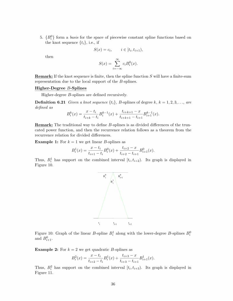
Example 1: For k = 1 we get linear B-splines as

B1i (x) =

x− titi+1 − ti

B0i (x) +

ti+2 − x

ti+2 − ti+1B0

i+1(x).

Thus, B1i has support on the combined interval [ti, ti+2). Its graph is displayed in

Figure 10.

i+2t

i+1t

it

1i

B

0i+1

B0i

B

Figure 10: Graph of the linear B-spline B1i along with the lower-degree B-splines B0

i

and B0i+1.

Example 2: For k = 2 we get quadratic B-splines as

B2i (x) =

x− titi+2 − ti

B1i (x) +

ti+3 − x

ti+3 − ti+1B1

i+1(x).

Thus, B2i has support on the combined interval [ti, ti+3). Its graph is displayed in

Figure 11.

36

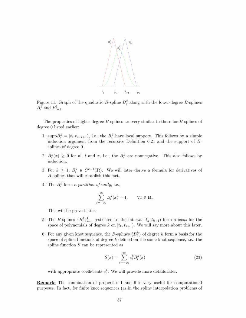
i+3t

i+2t

i+1t

it

2i

B

1i+1

B1i

B

Figure 11: Graph of the quadratic B-spline B2i along with the lower-degree B-splines

B1i and B1

i+1.

The properties of higher-degree B-splines are very similar to those for B-splines ofdegree 0 listed earlier:

1. suppBki = [ti, ti+k+1), i.e., the Bk

i have local support. This follows by a simpleinduction argument from the recursive Definition 6.21 and the support of B-splines of degree 0.

2. Bki (x) ≥ 0 for all i and x, i.e., the Bk

i are nonnegative. This also follows byinduction.

3. For k ≥ 1, Bki ∈ Ck−1(IR). We will later derive a formula for derivatives of

B-splines that will establish this fact.

4. The Bki form a partition of unity, i.e.,

∞∑i=−∞

Bki (x) = 1, ∀x ∈ IR .

This will be proved later.

5. The B-splines Bki k

i=0 restricted to the interval [tk, tk+1) form a basis for thespace of polynomials of degree k on [tk, tk+1). We will say more about this later.

6. For any given knot sequence, the B-splines Bki of degree k form a basis for the

space of spline functions of degree k defined on the same knot sequence, i.e., thespline function S can be represented as

S(x) =∞∑

i=−∞cki B

ki (x) (23)

with appropriate coefficients cki . We will provide more details later.

Remark: The combination of properties 1 and 6 is very useful for computationalpurposes. In fact, for finite knot sequences (as in the spline interpolation problems of

37

the previous section), the B-splines will form a finite-dimensional basis for the splinefunctions of degree k, and due to property 1 the linear system obtained by applyingthe interpolation conditions (1) to a (finite) B-spline expansion of the form (23) willbe banded and non-singular. Moreover, changing the data locally will only have a localeffect on the B-spline coefficients, i.e., only a few of the coefficients will change.

Evaluation of Spline Functions via B-Splines

We now fix k, and assume the coefficients cki are given. Then, using the recursion

of Definition 6.21 and an index transformation on the bi-infinite sum,

∞∑i=−∞

cki B

ki (x) =

∞∑i=−∞

cki

[x− ti

ti+k − tiBk−1

i (x) +ti+k+1 − x

ti+k+1 − ti+1Bk−1

i+1 (x)]

=∞∑

i=−∞cki

x− titi+k − ti

Bk−1i (x) +

∞∑i=−∞

cki

ti+k+1 − x

ti+k+1 − ti+1Bk−1

i+1 (x)︸ ︷︷ ︸=

∞∑i=−∞

cki−1

ti+k − x

ti+k − tiBk−1

i (x)

=∞∑

i=−∞

[cki

x− titi+k − ti

+ cki−1

ti+k − x

ti+k − ti

]︸ ︷︷ ︸

=: ck−1i

Bk−1i (x).

This gives us a recursion formula for the coefficients cki . We now continue the

recursion until the degree of the B-splines has been reduced to zero. Thus,

∞∑i=−∞

cki B

ki (x) =

∞∑i=−∞

ck−1i Bk−1

i (x)

= . . . =∞∑

i=−∞c0i B

0i (x) = c0

j ,

where j is the index such that x ∈ [tj , tj+1).The recursive procedure just described is known as deBoor algorithm. It is used to

evaluate a spline function S at the point x. In fact,

Theorem 6.22 Let

S(x) =∞∑

i=−∞cki B

ki (x)

with known coefficients cki . Then S(x) = c0

j , where j is such that x ∈ [tj , tj+1), and thecoefficients are computed recursively via

ck−1i = ck

i

x− titi+k − ti

+ cki−1

ti+k − x

ti+k − ti. (24)

Remark: The computation of the coefficients can be arranged in a triangular tableauwhere each coefficient is a convex combination of the two coefficients to its left (in the

38

same row, and the row below) as stated in (24):

ckj ck−1

j ck−2j · · · c1

j c0j

ckj−1 ck−1

j−1 ck−2j−1 · · · c1

j−1...

......

ckj−k+2 ck−1

j−k+2 ck−2j−k+2

ckj−k+1 ck−1

j−k+1

ckj−k

Now we are able to show the partition of unity property. Consider

S(x) =∞∑

i=−∞cki B

ki (x)

with all coefficients cki = 1. Then, from (24),

ck−1i = ck

i

x− titi+k − ti

+ cki−1

ti+k − x

ti+k − ti

=(x− ti) + (ti+k − x)

ti+k − ti= 1.

This relation holds throughout the entire de Boor algorithm so that

S(x) =∞∑

i=−∞Bk

i (x) = c0j = 1.

Derivatives of B-splines

Theorem 6.23 For any k ≥ 2

d

dxBk

i (x) =k

ti+k − tiBk−1

i (x)− k

ti+k+1 − ti+1Bk−1

i+1 (x). (25)

Remark: The derivative formula (25) also holds for k = 1 except at the knots x =ti, ti+1, ti+2, where B1

i is not differentiable.

Proof: By induction. The cases k = 1, 2 are done in homework problem 6.5.14. ♠

We are now able to establish the smoothness of B-splines.

Theorem 6.24 For k ≥ 1, Bki ∈ Ck−1(IR).

Proof: We use induction on k. The case k = 1 is clear. Now we assume the statementholds for k, and show it is also true for k + 1, i.e., we show Bk+1

i ∈ Ck(IR).From (25) we know d

dxBk+1i is a linear combination of Bk

i and Bki+1 which, by the

induction hypothesis are both in Ck−1(IR). Therefore, ddxBk+1

i ∈ Ck−1(IR), and thusBk+1

i ∈ Ck(IR). ♠

39

Remark: Simple integration formulas for B-splines also exist. See, e.g., page 373 ofthe textbook.

Linear Independence

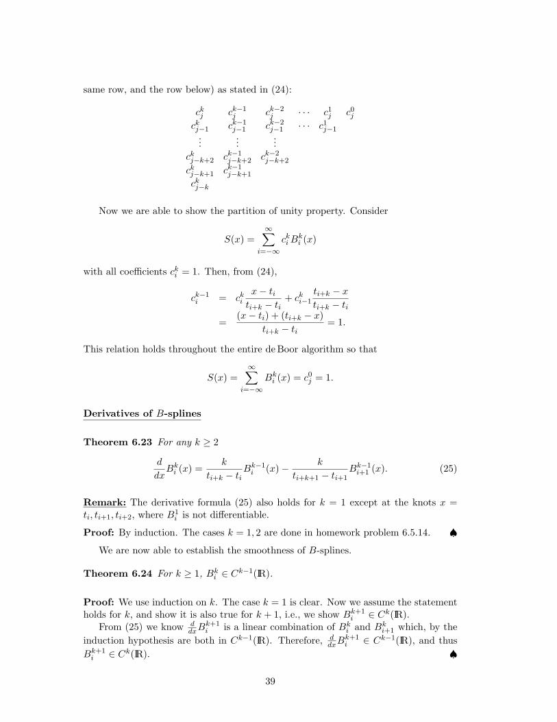
We now return to property 5 listed earlier. We will be slightly more general andconsider the set Bk

j , Bkj+1, . . . , B

kj+k of k + 1 B-splines of degree k.

Example 1: Figure 12 shows the two linear B-splines B1j and B1

j+1. From the figureit is clear that they are linearly independent on the intersection of their supports[tj+1, tj+2). Since the dimension of the space of linear polynomials (restricted to thisinterval) is two, and the two B-splines are linearly independent they form a basis forthe space of linear polynomials restricted to [tj+1, tj+2).

j+3t

j+2t

j+1t

jt

1j+1

B1j

B

Figure 12: Graph of the linear B-splines B1j and B1

j+1.

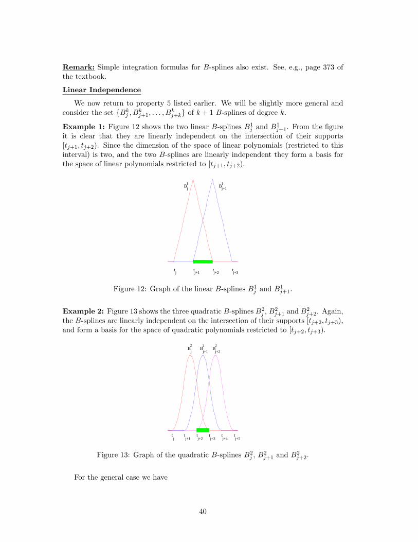
Example 2: Figure 13 shows the three quadratic B-splines B2j , B2

j+1 and B2j+2. Again,

the B-splines are linearly independent on the intersection of their supports [tj+2, tj+3),and form a basis for the space of quadratic polynomials restricted to [tj+2, tj+3).

j+5t

j+4t

j+3t

j+2t

j+1t

jt

2

j+2B

2

j+1B

2

jB

Figure 13: Graph of the quadratic B-splines B2j , B2

j+1 and B2j+2.

For the general case we have

40

Lemma 6.25 The set Bkj , Bk

j+1, . . . , Bkj+k of k + 1 B-splines of degree k is linearly

independent on the interval [tj+k, tj+k+1) and forms a basis for the space of polynomialsof degree k there.

Proof: By induction. See the textbook on page 373. ♠

Now we assume that we have a finite knot sequence t0, t1, . . . , tn (as we had inthe previous section on spline interpolation). Then we can find a finite-dimensionalbasis of B-splines of degree k for the space of spline functions of degree k defined onthe given knot sequence. As a first step in this direction we have

Lemma 6.26 Given a knot sequence t0, t1, . . . , tn, the set Bk−k, B

k−k+1, . . . , B

kn−1

of n + k B-splines of degree k is linearly independent on [t0, tn).

Proof: According to the definition of linear independence, we define a spline function

S(x) =n−1∑i=−k

ciBki (x),

and show that, for any x ∈ [t0, tn), S(x) = 0 is only possible if all coefficients ci,i = −k, . . . , n− 1, are zero.

The main idea is to break the interval [t0, tn) into smaller pieces [tj , tj+1) and showlinear independence on each of the smaller intervals.

If we consider the interval [t0, t1), then by Lemma 6.25 only the k + 1 B-splinesBk

−k, . . . , Bk0 are ”active” on this interval, and linearly independent there.

Therefore, restricted to [t0, t1) we have

S|[t0,t1) =0∑

i=−k

ciBki = 0 =⇒ ci = 0, i = −k, . . . , 0.

Similarly, we can argue that

S|[tj ,tj+1) =j∑

i=j−k

ciBki = 0 =⇒ ci = 0, i = j − k, . . . , j.

Now, for any x ∈ [tj , tj+1) the coefficients of all B-splines whose supports intersectthe interval are zero. Finally, since x is arbitrary, all coefficients must be zero. ♠

Remark: The representation of polynomials in terms of B-splines is given by Marsden’sidentity

∞∑i=−∞

k∏j=1

(ti+j − s)Bki (x) = (x− s)k.

This is covered in homework problems 6.5.9–12.

41

6.6 More B-Splines

We introduce the notation Skn for the space of spline functions of degree k defined on

the knot sequence t0, t1, . . . , tn. Our goal is to find a basis for Skn.

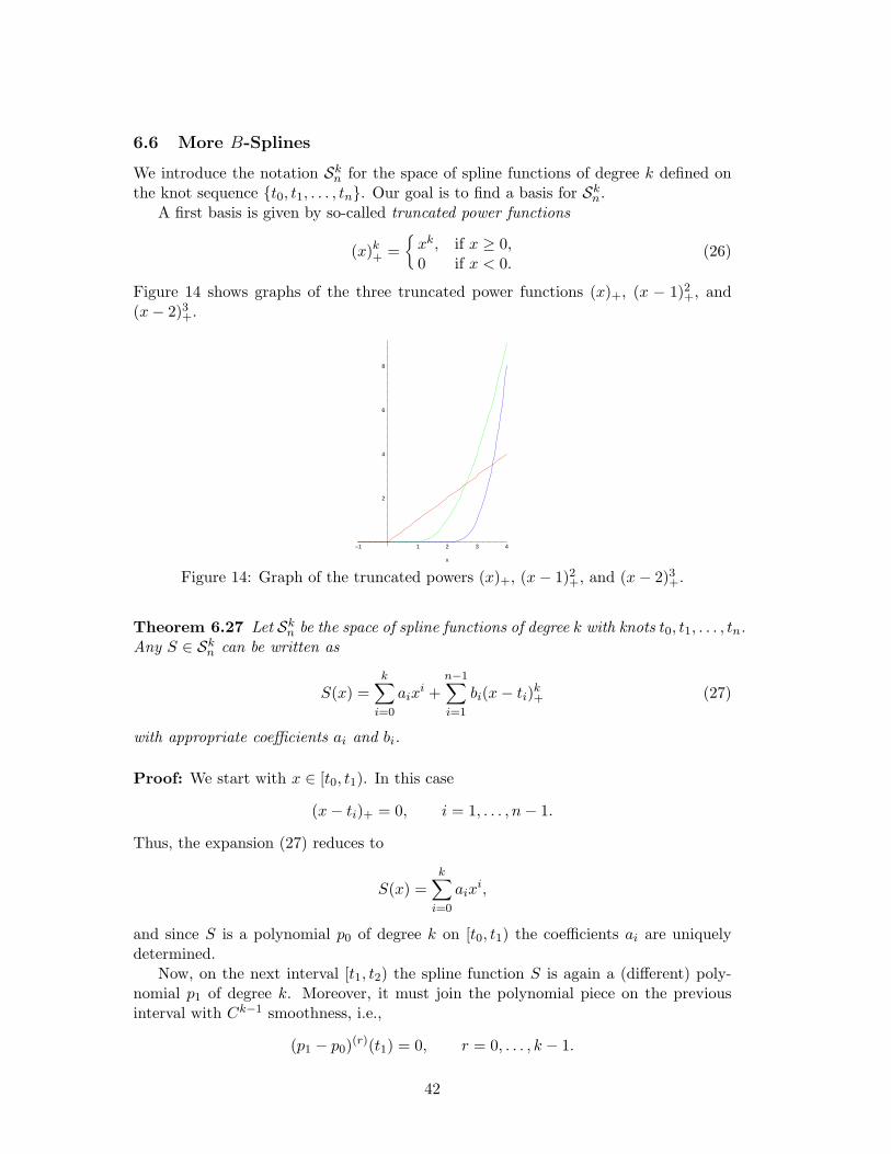
A first basis is given by so-called truncated power functions

(x)k+ =

xk, if x ≥ 0,0 if x < 0.

(26)

Figure 14 shows graphs of the three truncated power functions (x)+, (x − 1)2+, and(x− 2)3+.

2

4

6

8

–1 1 2 3 4

x

Figure 14: Graph of the truncated powers (x)+, (x− 1)2+, and (x− 2)3+.

Theorem 6.27 Let Skn be the space of spline functions of degree k with knots t0, t1, . . . , tn.

Any S ∈ Skn can be written as

S(x) =k∑

i=0

aixi +

n−1∑i=1

bi(x− ti)k+ (27)

with appropriate coefficients ai and bi.

Proof: We start with x ∈ [t0, t1). In this case

(x− ti)+ = 0, i = 1, . . . , n− 1.

Thus, the expansion (27) reduces to

S(x) =k∑

i=0

aixi,

and since S is a polynomial p0 of degree k on [t0, t1) the coefficients ai are uniquelydetermined.

Now, on the next interval [t1, t2) the spline function S is again a (different) poly-nomial p1 of degree k. Moreover, it must join the polynomial piece on the previousinterval with Ck−1 smoothness, i.e.,

(p1 − p0)(r)(t1) = 0, r = 0, . . . , k − 1.

42

Therefore, deg(p1 − p0) ≤ k, and we have the representation

(p1 − p0)(x) = b1(x− t1)k,

and

S(x) =k∑

i=0

aixi + b1(x− t1)k

+, x ∈ [t0, t2).

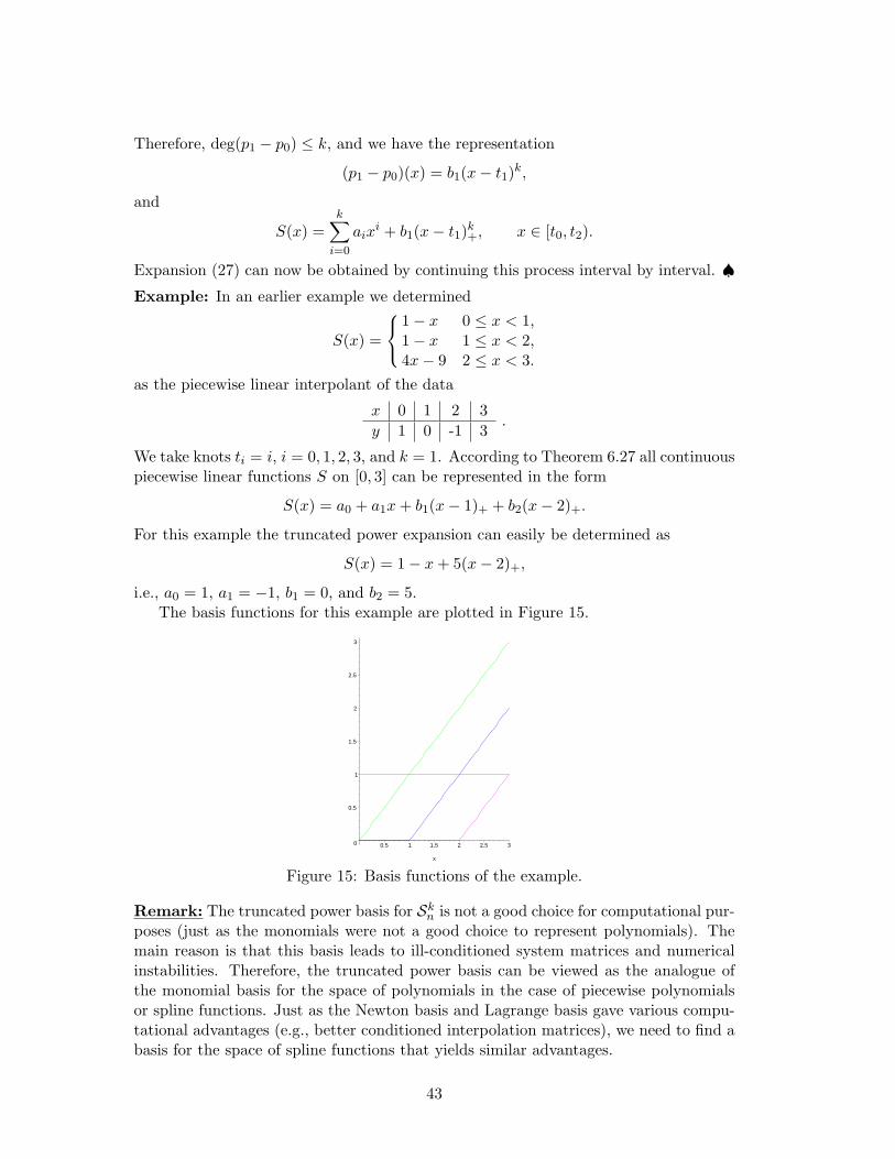
Expansion (27) can now be obtained by continuing this process interval by interval. ♠Example: In an earlier example we determined

S(x) =

1− x 0 ≤ x < 1,1− x 1 ≤ x < 2,4x− 9 2 ≤ x < 3.

as the piecewise linear interpolant of the data

x 0 1 2 3y 1 0 -1 3

.

We take knots ti = i, i = 0, 1, 2, 3, and k = 1. According to Theorem 6.27 all continuouspiecewise linear functions S on [0, 3] can be represented in the form

S(x) = a0 + a1x + b1(x− 1)+ + b2(x− 2)+.

For this example the truncated power expansion can easily be determined as

S(x) = 1− x + 5(x− 2)+,

i.e., a0 = 1, a1 = −1, b1 = 0, and b2 = 5.The basis functions for this example are plotted in Figure 15.

0

0.5

1

1.5

2

2.5

3

0.5 1 1.5 2 2.5 3

x

Figure 15: Basis functions of the example.

Remark: The truncated power basis for Skn is not a good choice for computational pur-

poses (just as the monomials were not a good choice to represent polynomials). Themain reason is that this basis leads to ill-conditioned system matrices and numericalinstabilities. Therefore, the truncated power basis can be viewed as the analogue ofthe monomial basis for the space of polynomials in the case of piecewise polynomialsor spline functions. Just as the Newton basis and Lagrange basis gave various compu-tational advantages (e.g., better conditioned interpolation matrices), we need to find abasis for the space of spline functions that yields similar advantages.

43

Corollary 6.28 The dimension of the space Skn of spline functions of degree k with

knots t0, t1, . . . , tn isdim Sk

n = n + k.

Proof: There are (k + 1) + (n− 1) = n + k basis functions in (27). ♠A Better Basis for Sk

n

Theorem 6.29 Any spline function S ∈ Skn can be represented with respect to the

B-spline basis Bk

i |[t0,tn] : i = −k, . . . , n− 1

. (28)

Proof: According to Corollary 6.28 we need n+k basis functions. The set (28) containsn + k functions in Sk

n, and according to Lemma 6.26 they are linearly independent on[t0, tn]. ♠

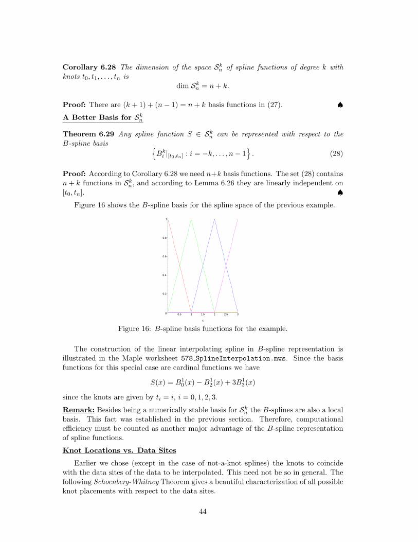
Figure 16 shows the B-spline basis for the spline space of the previous example.

0

0.2

0.4

0.6

0.8

1

0.5 1 1.5 2 2.5 3

x

Figure 16: B-spline basis functions for the example.

The construction of the linear interpolating spline in B-spline representation isillustrated in the Maple worksheet 578 SplineInterpolation.mws. Since the basisfunctions for this special case are cardinal functions we have

S(x) = B10(x)−B1

2(x) + 3B13(x)

since the knots are given by ti = i, i = 0, 1, 2, 3.

Remark: Besides being a numerically stable basis for Skn the B-splines are also a local

basis. This fact was established in the previous section. Therefore, computationalefficiency must be counted as another major advantage of the B-spline representationof spline functions.

Knot Locations vs. Data Sites

Earlier we chose (except in the case of not-a-knot splines) the knots to coincidewith the data sites of the data to be interpolated. This need not be so in general. Thefollowing Schoenberg-Whitney Theorem gives a beautiful characterization of all possibleknot placements with respect to the data sites.

44

Theorem 6.30 Assume x1 < x2 < . . . < xn and

S(x) =n∑

j=1

cjBkj (x),

We can use S to interpolate arbitrary data given at the points xi, i = 1, . . . , n, if andonly if the knots ti are chosen so that there is at least one data site xi in the supportof every B-spline.

Proof: The proof of this theorem is fairly complicated and long and presented in theform of Lemmas 1, 2 and Theorems 2 and 3 on pages 378–383 of the textbook. ♠

Remarks:

1. From an algebraic point of view, the Schoenberg-Whitney Theorem says that theinterpolation matrix B with entries Bk

j (xi) (cf. Section 6.0) should not have anyzeros on its diagonal.

2. Theorem 6.30 does not guarantee a unique interpolant. In fact, as we saw in theexamples for quadratic and cubic spline interpolation in Section 6.4, additionalconditions may be required to ensure uniqueness.

3. Common choices for the knot locations are

• For linear splines, choose ti = xi, i = 1, . . . , n.

• For k > 1, choose

– the knots at the node averages,– the nodes at the knot averages.

Example: We illustrate some possible relative knot placements in the Maple worksheet578 SplineInterpolation.mws.

Approximation by Splines

Recall that the Weierstrass Approximation Theorem states that any continuousfunction can be approximated arbitrarily closely by a polynomial (of sufficiently highdegree) on [a, b].

We will now show that splines (of fixed degree k, but with sufficiently many knots)do the same.

Definition 6.31 Let f be defined on [a, b].

ω(f ;h) = max|s−t|≤h

|f(s)− f(t)|

is called the modulus of continuity of f .

45

Remarks:

1. If f is continuous on [a, b], then it is also uniformly continuous there, i.e., for anyε > 0 there exists a δ > 0 such that for all s, t ∈ [a, b]

|s− t| < δ =⇒ |f(s)− f(t)| < ε.

Therefore, ω(f ; δ) = max|s−t|≤δ

|f(s)− f(t)| ≤ ε, and for any continuous f we have

ω(f ;h) → 0 as h → 0.

2. If f is Lipschitz continuous with Lipschitz constant λ on [a, b], i.e.,

|f(s)− f(t)| ≤ λ|s− t|,

then ω(f ;h) ≤ λh.

3. If f is differentiable with |f ′(t)| ≤ M on [a, b], then we also have ω(f ;h) ≤ Mh,but its rate of decay to zero as h → 0 depends on the maximum of the derivativeof f .

4. By comparing how fast ω(f ;h) tends to zero for h → 0 the modulus of continuityenables us to measure varying degrees of continuity.

An important property of the modulus of continuity is its so-called subadditivity,i.e.,

ω(f ; kh) ≤ kω(f ;h).

We will use this property below, and you will prove it in homework problem 6.6.20.

The approximation power of splines can be obtained from the following Whitney-type theorem.

Theorem 6.32 Let f be a function defined on [t0, tn], and assume knots . . . < t−2 <t−1 < t0 < t1 < t2 < . . . are given, such that

h = max−k≤i≤n+1

|ti − ti−1|

denotes the meshsize. Then the spline function

s(x) =∞∑

i=−∞f(ti+2)Bk

i (x)

satisfiesmax

t0≤x≤tn|f(x)− s(x)| ≤ kω(f ;h).

46

Remark: If k is fixed, then for a continuous f we have

ω(f ;h) → 0 as h → 0,

and therefore the Weierstrass-like approximation property of splines is established pro-vided we add sufficiently many knots to let the meshsize h go to zero.

Proof: Using the partition of unity property and nonnegativity of B-splines of degreek we have

|f(x)− s(x)| =∣∣∣f(x)

∞∑i=−∞

Bki (x)︸ ︷︷ ︸

=1

−∞∑

i=−∞f(ti+2)Bk

i (x)∣∣∣

≤∞∑

i=−∞|f(x)− f(ti+2)|Bk

i (x)︸ ︷︷ ︸≥0

.

Next we take j to be an index such that x ∈ [tj , tj+1). Then the bi-infinite sum can bereplaced by a finite sum over the active B-splines

|f(x)− s(x)| ≤j∑

i=j−k

|f(x)− f(ti+2)|Bki (x)

≤ maxj−k≤i≤j

|f(x)− f(ti+2)|j∑

i=j−k

Bki (x)

︸ ︷︷ ︸=1

.

Now, by the special choice of j we have x ≥ tj , as well as i ≤ j, and therefore

ti+2 − x ≤ tj+2 − tj ≤ 2h.

On the other hand, since x < tj+1 and i ≥ j − k

x− ti+2 ≤ tj+1 − tj−k+2 ≤ kh.

Summarizing, we have

maxj−k≤i≤j

|f(x)− f(ti+2)| ≤ max|x−ti+2|≤kh

|f(x)− f(ti+2)| = ω(f, kh),

and therefore, by the subadditivity of ω,

|f(x)− s(x)| ≤ ω(f ; kh) ≤ kω(f ;h).

♠

Remarks:

1. The error bound in Theorem 6.32 does not say anything about interpolatingsplines. However, similar results hold for that case also.

47

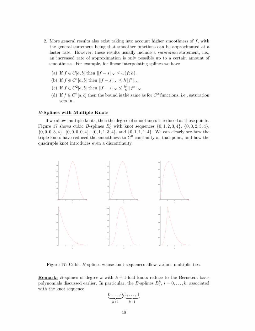
2. More general results also exist taking into account higher smoothness of f , withthe general statement being that smoother functions can be approximated at afaster rate. However, these results usually include a saturation statement, i.e.,an increased rate of approximation is only possible up to a certain amount ofsmoothness. For example, for linear interpolating splines we have

(a) If f ∈ C[a, b] then ‖f − s‖∞ ≤ ω(f ;h).

(b) If f ∈ C1[a, b] then ‖f − s‖∞ ≤ h‖f ′‖∞.

(c) If f ∈ C2[a, b] then ‖f − s‖∞ ≤ h2

8 ‖f′′‖∞.

(d) If f ∈ C3[a, b] then the bound is the same as for C2 functions, i.e., saturationsets in.

B-Splines with Multiple Knots

If we allow multiple knots, then the degree of smoothness is reduced at those points.Figure 17 shows cubic B-splines B3

0 with knot sequences 0, 1, 2, 3, 4, 0, 0, 2, 3, 4,0, 0, 0, 3, 4, 0, 0, 0, 0, 4, 0, 1, 1, 3, 4, and 0, 1, 1, 1, 4. We can clearly see how thetriple knots have reduced the smoothness to C0 continuity at that point, and how thequadruple knot introduces even a discontinuity.

0

0.1

0.2

0.3

0.4

0.5

0.6

1 2 3 4

x

0

0.1

0.2

0.3

0.4

0.5

1 2 3 4

x

0

0.1

0.2

0.3

0.4

0.5

1 2 3 4

x

0

0.2

0.4

0.6

0.8

1

1 2 3 4

x

0

0.1

0.2

0.3

0.4

0.5

0.6

1 2 3 4

x

0

0.2

0.4

0.6

0.8

1

1 2 3 4

x

Figure 17: Cubic B-splines whose knot sequences allow various multiplicities.

Remark: B-splines of degree k with k + 1-fold knots reduce to the Bernstein basispolynomials discussed earlier. In particular, the B-splines Bk

i , i = 0, . . . , k, associatedwith the knot sequence

0, . . . , 0︸ ︷︷ ︸k+1

, 1, . . . , 1︸ ︷︷ ︸k+1

48

are exactly the Bernstein basis polynomials(k

i

)xi(1− x)k−i (see, e.g., Figure 4 for the

case k = 3). This connection is heavily exploited in CAGD where Bezier curves canthereby be expressed in terms of B-splines (with multiple knots). More details aregiven, e.g., in the books by Farin, Hoschek and Lasser, and the new book ”Bezier andB-Spline Techniques” by Prautzsch, Boehm and Paluszny.

6.8 Best Approximation: Least Squares Theory

Given a normed linear space E and some function f ∈ E, as well as a subspace G ⊂ E(the so-called approximation space) the best approximation problem is to find a functiong ∈ G such that

‖f − g‖ → min.

A function g which minimizes this quantity is called the best approximation of f fromG.

We will consider E to be an inner product space with one of the following two innerproducts:

1. For f, g ∈ E with E = C[a, b] or E = L2[a, b]

〈f, g〉 =∫ b

af(x)g(x)w(x)dx

with w > 0 a continuous weight function.

2. For x, y ∈ E = IRn

〈x, y〉 =n∑

i=1

xiyi.

We restrict our attention to inner product spaces because it is easy to characterizebest approximation in those spaces.

Theorem 6.33 Let E be an inner product space. Then g ∈ G ⊂ E is a best approxi-mation to f ∈ E from G if and only if f − g ⊥ G.

Remark: The notation used in Theorem 6.33 is to be interpreted as

f − g ⊥ G ⇐⇒ 〈f − g, h〉 = 0 for all h ∈ G.

Proof: We recall the Pythagorean Theorem in an inner product space (see, e.g.,Lemma 5.6 in the Math 577 class notes, or page 274 of the textbook):

If f ⊥ g then ‖f + g‖2 = ‖f‖2 + ‖g‖2.

(a) ”⇐=”: We assume f − g ⊥ G, i.e., f − g ⊥ h for all h ∈ G. Let’s take an arbitraryh ∈ G. Then, using the Pythagorean Theorem,

‖f − h‖2 = ‖ f − g︸ ︷︷ ︸⊥G

+ g − h︸ ︷︷ ︸∈G

‖2

49

= ‖f − g‖2 + ‖g − h‖2︸ ︷︷ ︸≥0

≥ ‖f − g‖2,

and so g is a best approximation.(b) ”=⇒”: Now we assume g ∈ G is a best approximation to f . Then

‖f − g‖2 ≤ ‖f − (g + λh︸ ︷︷ ︸∈G

)‖2, λ > 0, h ∈ G

or‖f − g‖2 ≤ ‖f − g‖2 − 2λ〈f − g, h〉+ λ2‖h‖2.

This statement is equivalent to

0 ≤ λ2‖h‖2 − 2λ〈f − g, h〉= λ

(λ‖h‖2 − 2〈f − g, h〉

).

Thus, if λ → 0+, then we need to have 〈f − g, h〉 ≤ 0.Similarly – using −h instead of h – we can argue that 〈f − g, h〉 ≥ 0. Together we

have 〈f − g, h〉 = 0, and since h was arbitrary we have f − g ⊥ G. ♠

Remarks:

1. In an inner product space the best approximation is unique. This follows fromthe proof of Theorem 6.33.

2. If we take E = IR3 and G = IR2, then the best approximation g is given by theorthogonal projection of f onto G.

If we can obtain an orthonormal basis for G then

Theorem 6.34 Let g1, . . . , gn be an orthonormal basis of G ⊂ E. The best approx-imation g of f from G is a generalized Fourier series of the form

g =n∑

i=1

cigi

with generalized Fourier coefficients

ci = 〈f, gi〉.

Remark: The best approximation can be interpreted as the sum of the projections off onto the basis elements gi of G.

Proof: By the previous theorem the best approximation g is characterized by

f −n∑

i=1

cigi︸ ︷︷ ︸=g

⊥ G. (29)

50

We need to show that (29) is equivalent to the expression ci = 〈f, gi〉 for the Fouriercoefficients.

(29) implies that

f −n∑

i=1

cigi ⊥ gj , j = 1, . . . , n.

Therefore, taking the inner product with gj we have

〈f, gj〉 − 〈n∑

i=1

cigi, gj〉 = 0.

However,

〈n∑

i=1

cigi, gj〉 =n∑

i=1

ci 〈gi, gj〉︸ ︷︷ ︸δij

= cj ,

and therefore〈f, gj〉 − cj = 0.

♠

Theorem 6.35 (Parseval’s Identity) Let g1, . . . , gn be an orthonormal basis of G,and let g be the best approximation of f from G. Then

‖g‖2 =n∑

i=1

〈f, gi〉2.

Proof: By induction. First, note that the best approximation is given by the Fourierseries

g =n∑

i=1

〈f, gi〉gi.

For n = 1 this implies g = 〈f, g1〉g1. Therefore, since g1 is normalized,

‖g‖2 = ‖〈f, g1〉g1‖2 = 〈f, g1〉2 ‖g1‖2︸ ︷︷ ︸=1

.

Now, assume the statement holds for arbitrary n, show it is also true for n + 1.

‖g‖2 = ‖n+1∑i=1

〈f, gi〉gi‖2

= ‖n∑

i=1

〈f, gi〉gi + 〈f, gn+1〉gn+1‖2.

Since gn+1 is orthogonal to all of g1, . . . , gn, we can apply the Pythagorean Theoremand get

‖g‖2 = ‖n∑

i=1

〈f, gi〉gi‖2 + ‖〈f, gn+1〉gn+1‖2

51

=n∑

i=1

〈f, gi〉2 + 〈f, gn+1〉2 ‖gn+1‖2︸ ︷︷ ︸=1

=n+1∑i=1

〈f, gi〉2,

where we have used the induction hypothesis and the normalization of gn+1. ♠

Theorem 6.36 (Bessel’s Inequality) Let g1, . . . , gn be an orthonormal basis of G.Then

n∑i=1

〈f, gi〉2 ≤ ‖f‖2.

Proof: Consider the best approximation g to f . Now, by the Pythagorean Theorem,

‖f‖2 = ‖ f − g︸ ︷︷ ︸⊥G

+ g︸︷︷︸∈G

‖2

= ‖f − g‖2︸ ︷︷ ︸≥0

+‖g‖2

≥ ‖g‖2.

The proof is completed by applying Parseval’s identity. ♠

Remark: Given a linearly independent set h1, . . . , hn we can always obtain an or-thonormal set by applying the Gram-Schmidt method.

Best Approximation with Orthogonal Polynomials

We now take the approximation space G to be the space of polynomials of degree n,and show how one can find orthogonal bases for this approximation space (with respectto a specific inner product).

Theorem 6.37 Let 〈 , 〉 be an inner product. Any sequence of polynomials definedrecursively via

p0(x) = 1, p1(x) = x− a1,pn(x) = (x− an)pn−1(x)− bnpn−2(x), n ≥ 2

withan =

〈xpn−1, pn−1〉〈pn−1, pn−1〉

, bn =〈xpn−1, pn−2〉〈pn−2, pn−2〉

is orthogonal with respect to the inner product 〈 , 〉.

Proof: First note that all formulas are well-defined since all polynomials pn, n =0, 1, 2, . . . , are monic (and thus all denominators are nonzero). We use induction toshow that

〈pn, pi〉 = 0, i = 0, 1, . . . , n− 1. (30)

52

For the case n = 1 we use the definition of p0, p1 and a1 to get

〈p1, p0〉 = 〈x− a1, 1〉

= 〈x− 〈x, 1〉〈1, 1〉

, 1〉

= 〈x, 1〉 − 〈〈x, 1〉, 1〉〈1, 1〉

= 〈x, 1〉 − 〈x, 1〉 〈1, 1〉〈1, 1〉︸ ︷︷ ︸

=1= 0.

Now we assume that (30) holds for n, and show that it is also true for n+1. Using therecurrence relation we have

〈pn+1, pi〉 = 〈(x− an+1)pn − bn+1pn−1, pi〉= 〈xpn, pi〉 − an+1 〈pn, pi〉︸ ︷︷ ︸

=0

−bn+1 〈pn−1, pi〉︸ ︷︷ ︸=0

= 〈xpn, pi〉.

For any real inner product the last expression is equal to 〈pn, xpi〉. Next, the recurrencerelation (for n = i + 1) implies

pi+1(x) = (x− ai+1)pi(x)− bi+1pi−1(x)⇐⇒ xpi(x) = pi+1(x) + ai+1pi(x) + bi+1pi−1(x)

Therefore, we get

〈pn+1, pi〉 = 〈pn, pi+1 + ai+1pi + bi+1pi−1〉= 〈pn, pi+1〉︸ ︷︷ ︸

=0, i=0,1,...,n−2

+ai+1 〈pn, pi〉︸ ︷︷ ︸=0, i=0,1,...,n−1

+bi+1 〈pn, pi−1〉︸ ︷︷ ︸=0, i=0,1,...,n

= 0

for i = 0, 1, . . . , n− 2, and we still need to show

〈pn+1, pi〉 = 0 for i = n− 1, n.

For these two cases we apply the recurrence relation directly:

〈pn+1, pn−1〉 = 〈xpn, pn−1〉 − an+1 〈pn, pn−1〉︸ ︷︷ ︸=0

−bn+1〈pn−1, pn−1〉

= 〈xpn, pn−1〉 −〈xpn, pn−1〉〈pn−1, pn−1〉︸ ︷︷ ︸

=bn+1

〈pn−1, pn−1〉

= 0,

53

and

〈pn+1, pn〉 = 〈xpn, pn〉 − an+1〈pn, pn〉 − bn+1 〈pn−1, pn〉︸ ︷︷ ︸=0

= 〈xpn, pn〉 −〈xpn, pn〉〈pn, pn〉︸ ︷︷ ︸=an+1

〈pn, pn〉

= 0.

♠

Different families of orthogonal polynomials are now obtained by choosing an innerproduct, and then applying the recurrence relation. We now discuss the ”classical”orthogonal polynomials.

Example 1: Legendre polynomials. We take the inner product

〈f, g〉 =∫ 1

−1f(x)g(x)dx

We always start with p0(x) = 1. According to Theorem 6.37 we then have

p1(x) = x− a1

with

a1 =〈xp0, p0〉〈p0, p0〉

=

∫ 1

−1xdx∫ 1

−1dx

= 0,

so that p1(x) = x. Next,

p2(x) = (x− a2)p1(x)− b2p0(x),

with

a2 =〈xp1, p1〉〈p1, p1〉

=

∫ 1

−1x3dx∫ 1

−1x2dx

= 0

and

b2 =〈xp1, p0〉〈p0, p0〉

=

∫ 1

−1x2dx∫ 1

−1dx

=13,

so that p2(x) = x2 − 13 . Similarly, one can obtain

p3(x) = x3 − 35x,

p4(x) = x4 − 67x2 +

335

,

p5(x) = x5 − 109

x3 +521

x.

54

Example 2: The Chebyshev polynomials of the first kind are obtained via the innerproduct

〈f, g〉 =∫ 1

−1f(x)g(x)

1√1− x2

dx.

Remark: Recall that we encountered these polynomials when discussing optimal place-ment of data sites for polynomial interpolation.

Example 3: The Jacobi polynomials are obtained via the inner product

〈f, g〉 =∫ 1

−1f(x)g(x)(1− x)α(1 + x)βdx, α, β > −1.

Example 4: The Hermite polynomials are obtained via the inner product

〈f, g〉 =∫ ∞

−∞f(x)g(x)e−x2

dx.

Example 5: The Chebyshev polynomials of the second kind are obtained via the innerproduct

〈f, g〉 =∫ 1

−1f(x)g(x)

√1− x2dx.

Example 6: The Laguerre polynomials are obtained via the inner product

〈f, g〉 =∫ ∞

0f(x)g(x)xαe−xdx, α > −1.

Remarks:

1. The Maple worksheet 578 OrthogonalPolynomials.mws lists the first few (monic)polynomials of each type listed above.

2. Of course, the definition of Jacobi polynomials includes that of Legendre poly-nomials (for α = β = 0, Chebyshev polynomials of the first kind (α = β = −1

2),and Chebyshev polynomials of the second kind (α = β = 1

2).

Normal Equations and Gram Matrix

From above we know that the best approximation g to f from G is characterizedby f − g ⊥ G. In particular, if G has a basis g1, . . . , gn (orthogonal or not), then thebest approximation is characterized by

〈f − g, gi〉 = 0, i = 1, . . . , n.

Now g ∈ G, so

g =n∑

j=1

cjgj ,

and we have

〈f −n∑

j=1

cjgj , gi〉 = 0, i = 1, . . . , n.

55

By linearity we have

n∑j=1

cj〈gj , gi〉 = 〈f, gi〉, i = 1, . . . , n.

This is a system of linear equations of the form 〈g1, g1〉 . . . 〈gn, g1〉...

...〈g1, gn〉 . . . 〈gn, gn〉

︸ ︷︷ ︸

=G

c1...

cn

=

〈f, g1〉...

〈f, gn〉

, (31)

where G is a so-called Gram matrix. The system (31) is referred to as the normalequations of the least squares problem (cf. the earlier discussion in Sect.5.1).

Remarks:

1. If the set g1, . . . , gn is linearly independent, then the matrix G is nonsingular.This follows from the fact that g is the unique best least squares approxima-tion, and the fact that g has a unique representation with respect to the basisg1, . . . , gn.

2. If the set g1, . . . , gn is orthogonal, then G is diagonal. For an orthonormal basisG is even the identity matrix.

According to these remarks any basis of G can be used to compute g. However, anorthogonal basis leads to a trivial linear system. Other bases may lead to ill-conditionedGram matrices.

Example: Find the best least squares approximation from the space of quadraticpolynomials to f(x) = ex on [−1, 1].

First we use the monomial basis 1, x, x2, so that

g(x) =2∑

i=0

cixi.

The normal equations become 〈1, 1〉 〈x, 1〉 〈x2, 1〉〈1, x〉 〈x, x〉 〈x2, x〉〈1, x2〉 〈x, x2〉 〈x2, x2〉

c0

c1

c2

=

〈ex, 1〉〈ex, x〉〈ex, x2〉

.

Using the inner product

〈f, g〉 =∫ 1

−1f(x)g(x)dx

the system can be evaluated to 2 0 23

0 23 0

23 0 2

5

c0

c1

c2

=

e− 1e

2e

e− 5e

.

56

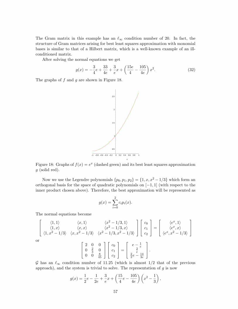
The Gram matrix in this example has an `∞ condition number of 20. In fact, thestructure of Gram matrices arising for best least squares approximation with monomialbases is similar to that of a Hilbert matrix, which is a well-known example of an ill-conditioned matrix.

After solving the normal equations we get

g(x) = −34e +

334e

+3ex +

(15e

4− 105

4e

)x2. (32)

The graphs of f and g are shown in Figure 18.

0.5

1

1.5

2

2.5

–1 –0.8 –0.6 –0.4 –0.2 0 0.2 0.4 0.6 0.8 1

x

Figure 18: Graphs of f(x) = ex (dashed green) and its best least squares approximationg (solid red).

Now we use the Legendre polynomials p0, p1, p2 = 1, x, x2− 1/3 which form anorthogonal basis for the space of quadratic polynomials on [−1, 1] (with respect to theinner product chosen above). Therefore, the best approximation will be represented as

g(x) =2∑

i=0

cipi(x).

The normal equations become 〈1, 1〉 〈x, 1〉 〈x2 − 1/3, 1〉〈1, x〉 〈x, x〉 〈x2 − 1/3, x〉

〈1, x2 − 1/3〉 〈x, x2 − 1/3〉 〈x2 − 1/3, x2 − 1/3〉

c0

c1

c2

=

〈ex, 1〉〈ex, x〉

〈ex, x2 − 1/3〉

or 2 0 0

0 23 0

0 0 845

c0

c1

c2

=

e− 1e

2e

23e− 14

3e

.

G has an `∞ condition number of 11.25 (which is almost 1/2 that of the previousapproach), and the system is trivial to solve. The representation of g is now

g(x) =12e− 1

2e+

3ex +

(154

e− 1054e

)(x2 − 1

3

),

57

which of course is equivalent to (32).

An alternative to continuous least squares approximation is

Discrete Least Squares Approximation

This method is useful when the data is given as a set of discrete points (xi, yi),i = 1, . . . , N , instead of as a function f . Now we want the best `2 approximation fromG.

Assuming that G has a basis g1, . . . , gn (usually with n N) we represent thebest approximation in the form

g =n∑

j=1

cjgj ,

and determine the unknown coefficients cj , j = 1, . . . , n, by minimizing the discrete `2

norm of the difference between the data and the best approximation, i.e.

N∑i=1

(yi − g(xi))2 =

N∑i=1

yi −n∑

j=1

cjgj(xi)

2

→ min.

Remarks:

1. A solution of this problem can be found (cf. Sect. 5.4.3 or Sect. 5.5.5) by comput-ing the QR or singular value decomposition of the Gram matrix G with entries

Gij = gj(xi), i = 1, . . . , N, j = 1, . . . , n.

An example involving polynomial discrete least squares approximation was pre-sented in Sect. 5.1.3 and the Matlab demo PolynomialDemo.m.

2. If n = N then we are back to the case of interpolation to the values yi at xi,i = 1, . . . , N .

3. If a set of linear constraints is added to the quadratic minimization problem thenthe Lagrange multiplier technique is used to convert the entire problem to a linearsystem.

4. We will return to discrete least squares approximation (with linear constraints)when we discuss the moving least squares method for approximation of multi-variate data.

6.9 Trigonometric Interpolation

This section can be found as Section 6.12 in the textbook.If we need to interpolate or approximate periodic functions or periodic data, then

it is more natural to use an approximation space consisting of periodic functions. Inthe case of continuous least squares approximation on [−π, π] this leads to classicalFourier series. The following theorem is proved in any standard undergraduate classon Fourier series.

58

Theorem 6.38 If f ∈ C1[−π, π] and f is 2π-periodic then its best approximation from

G = span1, cos x, cos 2x, . . . , sinx, sin 2x, . . .

is given by

f(x) ∼ g(x) =a0

2+

∞∑k=1

(ak cos kx + bk sin kx)

with

ak =1π

∫ π

−πf(t) cos ktdt,

bk =1π

∫ π

−πf(t) sin ktdt.

Moreover, g converges uniformly to f .

Complex Fourier Series

By employing Euler’s formula

eiφ = cos φ + i sinφ

the Fourier series approach can be unified. Then

f(x) ∼∞∑

k=−∞cke

ikx

withck =

12(ak − ibk) (a−k = ak, b−k = bk, b0 = 0).

This implies

ck =12π

∫ π

−πf(t) (cos kt− i sin kt) dt

=12π

∫ π

−πf(t)eiktdt = f(k)

and the coefficients ck = f(k) are referred to as the Fourier transform of f .

Remark: Just as 1, cos x, cos 2x, . . . , sinx, sin 2x, . . . are orthonormal with respect tothe inner product

〈f, g〉 =1π

∫ π

−πf(x)g(x)dx,

the functions eikx∞k=−∞ are orthonormal with respect to the (complex) inner product

〈f, g〉 =12π

∫ π

−πf(x)g(x)dx.

Let’s verify the statement just made. Let Ek be defined by

Ek(x) := eikx.

59

Then〈Ek, Ek〉 =

12π

∫ π

−πeikxe−ikx︸ ︷︷ ︸

=1

dx = 1.

For k 6= ` we have

〈Ek, E`〉 =12π

∫ π

−πeikxe−i`xdx

=12π

∫ π

−πei(k−`)xdx

=12π

ei(k−`)x

i(k − `)

∣∣∣∣∣π

−π

=1

2πi(k − `)

[ei(k−`)π − e−i(k−`)π

]=

12πi(k − `)

ei(k−`)π

1− e2π(`−k)i︸ ︷︷ ︸=1

= 0.

In order to discuss discrete least squares approximation or interpolation with trigono-metric functions we introduce

Exponential Polynomials

Let

P (x) =n∑

k=0

ckEk(x).

Since we can write

P (x) =n∑

k=0

ckeikx =

n∑k=0

ck

(eix)k

P is a polynomial of degree k in the complex exponential eix.For discrete least squares approximation we now consider equally spaced data on

the interval [0, 2π), i.e.,

(xj , f(xj)) with xj =2πj

N, j = 0, 1, . . . , N − 1, (33)

and introduce a discrete (pseudo-)inner product

〈f, g〉N =1N

N−1∑j=0

f

(2πj

N

)g

(2πj

N

). (34)

Remark: This is only a pseudo-inner product since 〈f, f〉N = 0 implies f = 0 only atthe discrete nodes 2πj

N , j = 0, 1, . . . , N − 1.

Theorem 6.39 The set EkN−1k=0 of complex exponentials is orthonormal with respect

to the inner product 〈 , 〉N defined in (34).

60

Proof: First,

〈Ek, Ek〉N =1N

N−1∑j=0

Ek

(2πj

N

)Ek

(2πj

N

)

=1N

N−1∑j=0

eik2πj/Ne−ik2πj/N︸ ︷︷ ︸=1

= 1.

Next, for k 6= ` we have

〈Ek, E`〉N =1N

N−1∑j=0

Ek

(2πj

N

)E`

(2πj

N

)

=1N

N−1∑j=0

eik2πj/Ne−i`2πj/N

=1N

N−1∑j=0

(ei

2π(k−`)N

)j

.

Now, since k 6= `,ei

2π(k−`)N 6= 1

we can apply the formula for the sum of a finite geometric series to get

〈Ek, E`〉N =1N

(ei

2π(k−`)N

)N

− 1

ei2π(k−`)

N − 1.

Finally, since (ei

2π(k−`)N

)N

= 1

the orthogonality result follows. ♠

Corollary 6.40 Let data be given as in (33) and consider G = spanEknk=0 with

n < N . Then the best least squares approximation to the data from G (with respect tothe inner product (34)) is given by the discrete Fourier series

g(x) =n∑

k=0

ckEk(x)

with

ck = 〈f,Ek〉N =1N

N−1∑j=0

f

(2πj

N

)e−ik 2πj

N , k = 0, 1, . . . , n.

Proof: This follows immediately from the orthonormality of Eknk=0 and from Theo-

rem 6.34 on generalized Fourier series. ♠

61

Remarks:

1. The coefficients ck of the discrete Fourier series are called the discrete Fouriertransform (DFT) of f .

2. In the next section we will compute the DFT (and also evaluate g) via the fastFourier transform (FFT).

3. Note that, even if the data is real, the DFT will in general be complex. If, e.g.,N = 4, and the values f

(2πjN

), j = 0, 1, 2, 3 are 4, 0, 3, 6 respectively, then the

coefficients ck are

c0 = 13c1 = 1 + 6ic2 = 1c3 = 1− 6i.

Corollary 6.41 Let data be given as in (33), then the exponential polynomial

P (x) =N−1∑k=0

〈f,Ek〉NEk(x)

is the unique interpolant to the data from G = spanEkN−1k=0 .

Proof: Apply Corollary 6.40 with n = N − 1. ♠

Remark: The DFT can be interpreted as a matrix-vector product with matrix E whoseentries are given by

Ejk = e−ik 2πjN ,

which can be computed in O(N2) operations. On the other hand, the DFT yields aninterpolant to the given data, and interpolation problems usually require solution of alinear system (at O(N3) cost). Thus, the DFT (even if implemented naively) yields animprovement of one order of magnitude.

Example: Consider the data

x 0 π

y f(0) f(π).

We therefore have N = 2, and according to Corollary 6.41 the unique interpolant fromspanE0, E1 is given by

P (x) =1∑

k=0

ckEk(x)

= 〈f,E0〉2E0(x) + 〈f,E1〉2E1(x)

=12

1∑j=0

f

(2πj

2

)e−i0 2πj

2︸ ︷︷ ︸=1

ei0x︸︷︷︸=1

+12

1∑j=0

f

(2πj

2

)e−i 2πj

2

eix

62

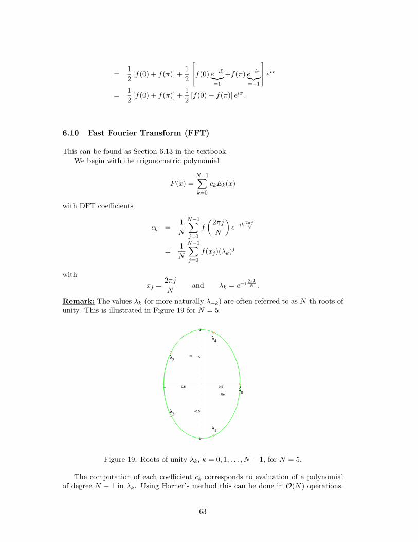
=12

[f(0) + f(π)] +12

f(0) e−i0︸︷︷︸=1

+f(π) e−iπ︸︷︷︸=−1

eix

=12

[f(0) + f(π)] +12

[f(0)− f(π)] eix.

6.10 Fast Fourier Transform (FFT)

This can be found as Section 6.13 in the textbook.We begin with the trigonometric polynomial

P (x) =N−1∑k=0

ckEk(x)

with DFT coefficients

ck =1N

N−1∑j=0

f

(2πj

N

)e−ik 2πj

N

=1N

N−1∑j=0

f(xj)(λk)j

withxj =

2πj

Nand λk = e−i 2πk

N .

Remark: The values λk (or more naturally λ−k) are often referred to as N -th roots ofunity. This is illustrated in Figure 19 for N = 5.

4λ

3λ

2λ

1λ

0λ

–1

–0.5

0.5

1

Im

–1 –0.5 0.5 1

Re

Figure 19: Roots of unity λk, k = 0, 1, . . . , N − 1, for N = 5.

The computation of each coefficient ck corresponds to evaluation of a polynomialof degree N − 1 in λk. Using Horner’s method this can be done in O(N) operations.

63

Since we have N coefficients, the polynomial P can be constructed inO(N2) operations.(Earlier we saw a matrix-vector multiplication argument to the same effect.)

The major benefit of the fast Fourier transform is that it reduces the amount ofwork to O(N log2 N) operations.

The FFT was discovered by Cooley and Tukey in 1965. However, Gauss seemed toalready be aware of similar ideas. One of the most popular modern references is the”DFT Owners Manual” by Briggs and Henson (published by SIAM in 1995). It is thedramatic reduction in computational complexity that earned the FFT a spot on thelist of ”Top 10 Algorithms of the 20th Century” (see handout).

The FFT is based on the following observation:

Theorem 6.42 Let data (xk, f(xk)), xk = kπn , k = 0, 1, . . . , 2n − 1, be given, and

assume that p and q are exponential polynomials of degree at most n−1 which interpolatepart of the data according to

p(x2j) = f(x2j), q(x2j) = f(x2j+1), j = 0, 1, . . . , n− 1,

then the exponential polynomial of degree at most 2n−1 which interpolates all the givendata is

P (x) =12

(1 + einx

)p(x) +

12

(1− einx

)q

(x− π

n

). (35)

Proof: Since einx =(eix)n has degree n, and p and q have degree at most n − 1 it is

clear that P has degree at most 2n− 1.We need to verify the interpolation claim, i.e., show that

P (xk) = f(xk), k = 0, 1, . . . , 2n− 1.

By assumption we have

P (xk) =12

(1 + einxk

)p(xk) +

12

(1− einxk

)q

(xk −

π

n

)where

einxk = ein kπn =

(eiπ)k

= (−1)k.

ThereforeP (xk) =

p(xk) if k even,q(xk − π

n

)if k odd.

Let k be even, i.e., k = 2j. Then, by the assumption on p

P (x2j) = p(x2j) = f(x2j), j = 0, 1, . . . , n− 1.

On the other hand, for k = 2j + 1 (odd), we have (using the assumption on q)

P (x2j+1) = q

(x2j+1 −

π

n

)= q(x2j) = f(x2j+1), j = 0, 1, . . . , n− 1.

This is true sincex2j+1 −

π

n=

(2j + 1)πn

− π

n=

2jπ

n= x2j .

♠The second useful fact tells us how to obtain the coefficients of P from those of p

and q.

64

Theorem 6.43 Let

p =n−1∑j=0

αjEj , q =n−1∑j=0

βjEj , and P =2n−1∑j=0

γjEj .

Then, for j = 0, 1, . . . , n− 1,

γj =12αj +

12e−ijπ/nβj

γj+n =12αj −

12e−ijπ/nβj .

Proof: In order to use (35) we need to rewrite

q

(x− π

n

)=

n−1∑j=0

βjEj

(x− π

n

)

=n−1∑j=0

βjeij(x−π

n)

=n−1∑j=0

βjeijxe−ijπ/n.

Therefore

P (x) =12

(1 + einx

)p(x) +

12

(1− einx

)q

(x− π

n

)=

12

n−1∑j=0

(1 + einx

)αje

ijx +12

n−1∑j=0

(1− einx

)βje

ijxe−ijπ/n

=12

n−1∑j=0

[(αj + βje

−ijπ/n)

eijx +(αj − βje

−ijπ/n)

ei(n+j)x].

However, the terms in parentheses (together with the factor 1/2) lead precisely to theformulæ for the coefficients γ. ♠

Example 1: As in the previous example, we consider the data

x 0 π

y f(0) f(π).

Now we apply the DFT to find the interpolating polynomial P . We have n = 1 and

P (x) =1∑

j=0

γjEj(x) = γ0e0 + γ1e

ix.

According to Theorem 6.43 the coefficients are given by

γ0 =12

(α0 + β0e

0)

,

γ1 =12

(α0 − β0e

0)

.

65

Therefore, we still need to determine α0 and β0. They are found via interpolation atonly one point (cf. Theorem 6.42):

p(x) =0∑

j=0

αjEj(x) = α0 such that p(x0) = f(x0) =⇒ α0 = f(x0)

q(x) =0∑

j=0

βjEj(x) = β0 such that q(x0) = f(x1) =⇒ β0 = f(x1).

With x0 = 0 and x1 = π we obtain

P (x) =12

(f(0) + f(π)) +12

(f(0)− f(π)) eix

which is the same as we computed earlier.

Example 2: We now refine the previous example, i.e., we consider the data

x 0 π2 π 3π

2

y f(0) f(

π2

)f(π) f

(3π2

) .

Now n = 2, and P is of the form

P (x) =3∑

j=0

γjEj(x).

According to Theorem 6.43 the coefficients are given by

γ0 =12

(α0 + β0) ,

γ1 =12

(α1 + β1 e−iπ/2︸ ︷︷ ︸

=−i

),

γ2 =12

(α0 − β0) ,

γ3 =12

(α1 − β1 e−iπ/2︸ ︷︷ ︸

=−i

).

This leaves the coefficients α0, β0 and α1, β1 to be determined. They are found viainterpolation at two points (cf. Theorem 6.42):

p(x) =1∑

j=0

αjEj(x) such that p(x0) = f(x0), p(x2) = f(x2),

q(x) =1∑

j=0

βjEj(x) such that q(x0) = f(x1), q(x2) = f(x3).

These are both problems of the form dealt with in the previous example, so a recursivestrategy is suggested.

A general recursive algorithm for the FFT is given in the textbook on pages 455and 456.

66

Computational Complexity

Assume N(= 2n) = 2m so that the recursive strategy for the FFT can be directlyapplied. (If N is not a power of 2, then the data can be padded appropriately withzeros). In order to evaluate the interpolating exponential polynomial

P (x) =N−1∑k=0

ckEk(x) =2n−1∑j=0

γjEj(x)

we can use the FFT to compute the coefficients ck (or γj).Instead of giving an exact count of the arithmetic operations involved in this task, we

estimate the minimum number of multiplications required to compute the coefficientsof an exponential polynomial with N terms.

Lemma 6.44 Let R(N) be the minimum number of multiplications required to computethe coefficients of an exponential polynomial with N = 2n terms. Then

R(N) ≤ 2R(n) + 2n.

Proof: There are N coefficients γj computed recursively via the formulas

γj =12αj +

12e−ijπ/nβj

γj+n =12αj −

12e−ijπ/nβj

listed in Theorem 6.43. If the factors 12e−ijπ/n, n = 0, 1, . . . , n − 1, are pre-computed,

then each of these formulas involves 2 multiplications for a total of 2n multiplications.Moreover, the coefficients αj and βj are determined recursively using R(n) multiplica-tions each. ♠

Theorem 6.45 Under the same assumptions as in Lemma 6.44 we have

R(2m) ≤ m2m.

Proof: We use induction on m. For m = 0 there are no multiplications since P (x) = c0.Now, assume the inequality holds for m. Then, by Lemma 6.44 (with n = 2m)

R(2m+1

)= R (2 · 2m) ≤ 2R (2m) + 2 · 2m.

By the induction hypothesis this is less than or equal to

2m2m + 2 · 2m = (m + 1)2m+1.

♠Setting N = 2m ⇔ m = log2 N in Theorem 6.45 implies

R(N) ≤ N log2 N,

i.e., the fast Fourier transform reduces the amount of computation required to evaluatean exponential polynomial fromO(N2) (if done directly) toO(N log2 N). For N = 1000this means roughly 104 instead of 106 operations.

67

Remarks:

1. Application of the classical fast Fourier transform is limited to the case where thedata is equally spaced, periodic, and of length 2m. The often suggested strategyof padding with zeros (to get a data vector of length 2m) or the application ofthe FFT to non-periodic data may produce unwanted noise.

2. Very recently, a version of the FFT for non-equally spaced data has been proposedby Daniel Potts, Gabriele Steidl and Manfred Tasche.

Remark: Given a vector a = [a0, a1, . . . , aN−1]T of discrete data, Corollary 6.40 tellsus that the discrete Fourier transform a of a is computed componentwise as

ak =1N

N−1∑j=0

aje−ik 2πj

N , k = 0, 1, . . . , N − 1.

Of course, the FFT can be used to compute these coefficients. There is an analogousformula for the inverse DFT, i.e.,

aj =N−1∑k=0

akeik 2πj

N , j = 0, 1, . . . , N − 1.

We close with a few applications of the FFT. Use of the FFT for many applica-tions benefits from the fact that convolution in the function domain corresponds tomultiplication in the transform domain, i.e.,

f ∗ g = f g

so that we havef ∗ g =

(f g)

.

Some applications are now

• Filters in signal or image processing.

• Compression of audio of video signals. E.g., the MP3 file format makes use ofthe discrete cosine transform.

• De-noising of data contaminated with measurement error (see, e.g., the Mapleworksheet 578 FFT.mws).

• Multiplication with cyclic matrices. A cyclic matrix is of the form

C =

a0 a1 . . . an−1 an

an a0 a1 . . . an−1

an−1 an a0 a1 . . .. . . . . . . . . . . . . . .a1 . . . an−1 an a0

68

and multiplication by C corresponds to a discrete convolution, i.e.,

(Cy)i =n∑

j=0

Cijyj =n∑

j=0

aj−iyj , i = 0, . . . , n,

where the subscript on a is to be interpreted cyclically, i.e., an+1+i ≡ ai ora−i ≡ an+1−i. Thus, a coupled system of linear equations with cyclic systemmatrix can be decoupled (and thus trivially solved) by applying the discreteFourier transform.

• High precision integer arithmetic also makes use of the FFT.

• Numerical solution of differential equations.

Remark: Another transform technique that has some similarities to (but also somesignificant differences from) the FFT is the fast wavelet transform. Using so-calledscaling functions and associated wavelets as orthogonal basis functions one can alsoperform best approximation of functions (or data). An advantage of wavelets over thetrigonometric basis used for the FFT is the fact that not only do we have localizationin the transform domain, but also in the function domain.

6.11 Multivariate Interpolation and Approximation

We now briefly turn our attention to some methods that can be used to interpolate orapproximate multivariate data, i.e., data of the form

(xi, f(xi)), i = 1, . . . , n, where xi ∈ Ω ⊂ IRd, and f(xi) ∈ IR .

Some of the methods discussed will be for the case d = 2 only, others will work forarbitrary d. The corresponding section in the textbook is 6.10.

Multivariate interpolation and approximation is still an active research area, andonly very few books on the subject are available:

1. C. K. Chui, Multivariate Splines, SIAM 1988,

2. P. Lancaster & K. Salkauskas, Curve and Surface Fitting, 1986,

3. W. Cheney & W. Light, A Course in Approximation Theory, 1999,

4. K. Hollig, Finite Element Methods with B-Splines, SIAM 2002,

5. G. R. Liu, Mesh Free Methods, 2003,

6. manuscripts by M. J. Lai & L. L. Schumaker on bivariate splines, and H. Wend-land on radial basis functions,

7. as well as several books in the CAGD literature, e.g., by Farin, Hoschek & Lasser.

69

As in the univariate case, we want to fit the given data with a function s from someapproximation space S with basis B1, . . . , Bm, i.e., s will be of the form

s(x) =m∑

j=1

cjBj(x), x ∈ IRd .

Depending on whether m = n or m < n, the coefficients cj (∈ IR) are then determinedby interpolation or some form of least squares approximation.

The fundamental difference between univariate and multivariate interpolation is thefollowing theorem on non-interpolation due to Mairhuber and Curtis (1956).

Theorem 6.46 If Ω ⊂ IRd, d ≥ 2, contains an interior point, then there exist no Haarspaces of continuous functions except for one-dimensional ones.

In order to understand this theorem we need

Definition 6.47 Let u1, . . . , un be a basis of the function space U . Then U is a Haarspace if

det (uj(xi)) 6= 0

for any set of distinct x1, . . . ,xn in Ω.

Remarks:

1. Note that existence of a Haar space guarantees invertibility of the interpolationmatrix (uj(xi)), i.e., existence and uniqueness of an interpolant to data specifiedat x1, . . . ,xn, from the space U .

2. In the univariate setting we know that polynomials of degree n − 1 form ann-dimensional Haar space for data given at x1, . . . , xn.

3. The Mairhuber-Curtis Theorem implies that in the multivariate setting we canno longer expect this to be the case. E.g., it is not possible to perform unique in-terpolation with (multivariate) polynomials of degree n to data given at arbitrarylocations in IR2.

4. Below we will look at a few constellations of data sites for which unique interpo-lation with bivariate polynomials is possible.

Proof of Theorem 6.46: Let d ≥ 2 and suppose U is a Haar space with basisu1, . . . , un with n ≥ 2. Then, by the definition of a Haar space

det (uj(xi)) 6= 0 (36)

for any distinct x1, . . . ,xn.Now consider a closed path P in Ω connecting only x1 and x2. This is possible

since – by assumption – Ω contains an interior point. We can exchange the positionsof x1 and x2 by moving them continuously along the path P (without interfering withany of the other xj). This means, however, that rows 1 and 2 of the determinant (36)have been exchanged, and so the determinant has changed sign.

Since the determinant is a continuous function of x1 and x2 we must have haddet = 0 at some point along P . This is a contradiction. ♠

70

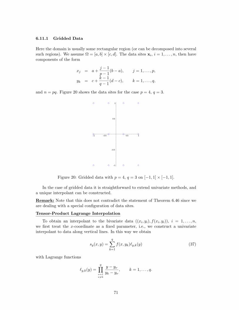
6.11.1 Gridded Data

Here the domain is usually some rectangular region (or can be decomposed into severalsuch regions). We assume Ω = [a, b]× [c, d]. The data sites xi, i = 1, . . . , n, then havecomponents of the form

xj = a +j − 1p− 1

(b− a), j = 1, . . . , p,

yk = c +k − 1q − 1

(d− c), k = 1, . . . , q,

and n = pq. Figure 20 shows the data sites for the case p = 4, q = 3.

–1

–0.5

0.5

1

–1 –0.5 0.5 1

Figure 20: Gridded data with p = 4, q = 3 on [−1, 1]× [−1, 1].

In the case of gridded data it is straightforward to extend univariate methods, anda unique interpolant can be constructed.

Remark: Note that this does not contradict the statement of Theorem 6.46 since weare dealing with a special configuration of data sites.

Tensor-Product Lagrange Interpolation

To obtain an interpolant to the bivariate data ((xi, yi), f(xi, yi)), i = 1, . . . , n,we first treat the x-coordinate as a fixed parameter, i.e., we construct a univariateinterpolant to data along vertical lines. In this way we obtain

sy(x, y) =q∑

k=1

f(x, yk)`y,k(y) (37)

with Lagrange functions

`y,k(y) =q∏

ν=1ν 6=k

y − yν

yk − yν, k = 1, . . . , q.

71

Note that due to the cardinality property of the Lagrange functions, sy interpolatesdata of the type

f(x, yk), k = 1, . . . , q.

Now we vary x and sample the (partial) interpolant sy to get the remaining data for a(nested) Lagrange interpolant to all of our data of the form

s(x, y) =p∑

j=1

sy(xj , y)`x,j(x) (38)

with Lagrange functions

`x,j(x) =p∏

ν=1ν 6=j

x− xν

xj − xν, j = 1, . . . , p.

Inserting (37) into (38) we obtain

s(x, y) =p∑

j=1

q∑k=1

f(xj , yk)`x,j(x)`y,k(y),

which is one representation of the tensor-product polynomial interpolant to the givendata.

Remarks:

1. Of course, we could have first constructed an interpolant sx to horizontal linedata, and then interpolated sx at the vertical locations – with the same endresult.

2. This method is illustrated in the Maple worksheet 578 TP Lagrange.mws.

3. Any univariate interpolation (or approximation) method of the form

s(x) =p∑

j=1

cjBj(x)

can be used to construct a tensor-product fit

s(x, y) =p∑

j=1

q∑k=1

cjkBj(x)Bk(y).

For example, if the data sets are large, then tensor-products of splines are pre-ferred over tensor-products of polynomials.

Boolean Sum Lagrange Interpolation

In the Boolean sum approach we need data given along curves x = const. andy = const. (or we have to generate that data from the given point data). We thencreate two independent univariate interpolants of the form

sx(x, y) =p∑

j=1

f(xj , y)`x,j(x),

72

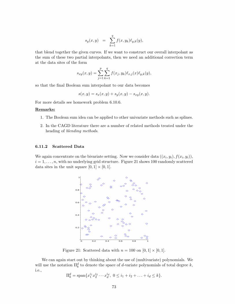
sy(x, y) =q∑

k=1

f(x, yk)`y,k(y),

that blend together the given curves. If we want to construct our overall interpolant asthe sum of these two partial interpolants, then we need an additional correction termat the data sites of the form

sxy(x, y) =p∑

j=1

q∑k=1

f(xj , yk)`x,j(x)`y,k(y),

so that the final Boolean sum interpolant to our data becomes

s(x, y) = sx(x, y) + sy(x, y)− sxy(x, y).

For more details see homework problem 6.10.6.

Remarks:

1. The Boolean sum idea can be applied to other univariate methods such as splines.

2. In the CAGD literature there are a number of related methods treated under theheading of blending methods.

6.11.2 Scattered Data

We again concentrate on the bivariate setting. Now we consider data ((xi, yi), f(xi, yi)),i = 1, . . . , n, with no underlying grid structure. Figure 21 shows 100 randomly scattereddata sites in the unit square [0, 1]× [0, 1].

0.2

0.4

0.6

0.8

1

0 0.2 0.4 0.6 0.8 1

Figure 21: Scattered data with n = 100 on [0, 1]× [0, 1].

We can again start out by thinking about the use of (multivariate) polynomials. Wewill use the notation Πd

k to denote the space of d-variate polynomials of total degree k,i.e.,

Πdk = spanxi1

1 xi22 · · ·x

idd , 0 ≤ i1 + i2 + . . . + id ≤ k.

73

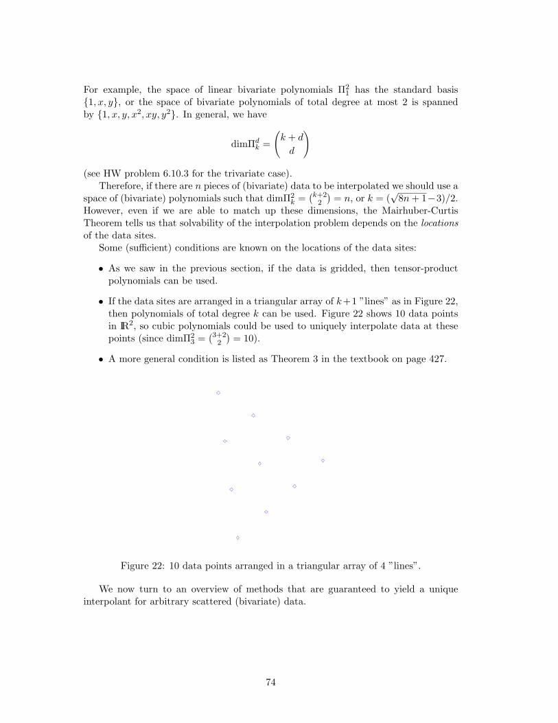
For example, the space of linear bivariate polynomials Π21 has the standard basis

1, x, y, or the space of bivariate polynomials of total degree at most 2 is spannedby 1, x, y, x2, xy, y2. In general, we have

dimΠdk =

(k + d

d

)

(see HW problem 6.10.3 for the trivariate case).Therefore, if there are n pieces of (bivariate) data to be interpolated we should use a

space of (bivariate) polynomials such that dimΠ2k =

(k+22

)= n, or k = (

√8n + 1−3)/2.

However, even if we are able to match up these dimensions, the Mairhuber-CurtisTheorem tells us that solvability of the interpolation problem depends on the locationsof the data sites.

Some (sufficient) conditions are known on the locations of the data sites:

• As we saw in the previous section, if the data is gridded, then tensor-productpolynomials can be used.

• If the data sites are arranged in a triangular array of k+1 ”lines” as in Figure 22,then polynomials of total degree k can be used. Figure 22 shows 10 data pointsin IR2, so cubic polynomials could be used to uniquely interpolate data at thesepoints (since dimΠ2

3 =(3+2

2

)= 10).

• A more general condition is listed as Theorem 3 in the textbook on page 427.

Figure 22: 10 data points arranged in a triangular array of 4 ”lines”.

We now turn to an overview of methods that are guaranteed to yield a uniqueinterpolant for arbitrary scattered (bivariate) data.

74

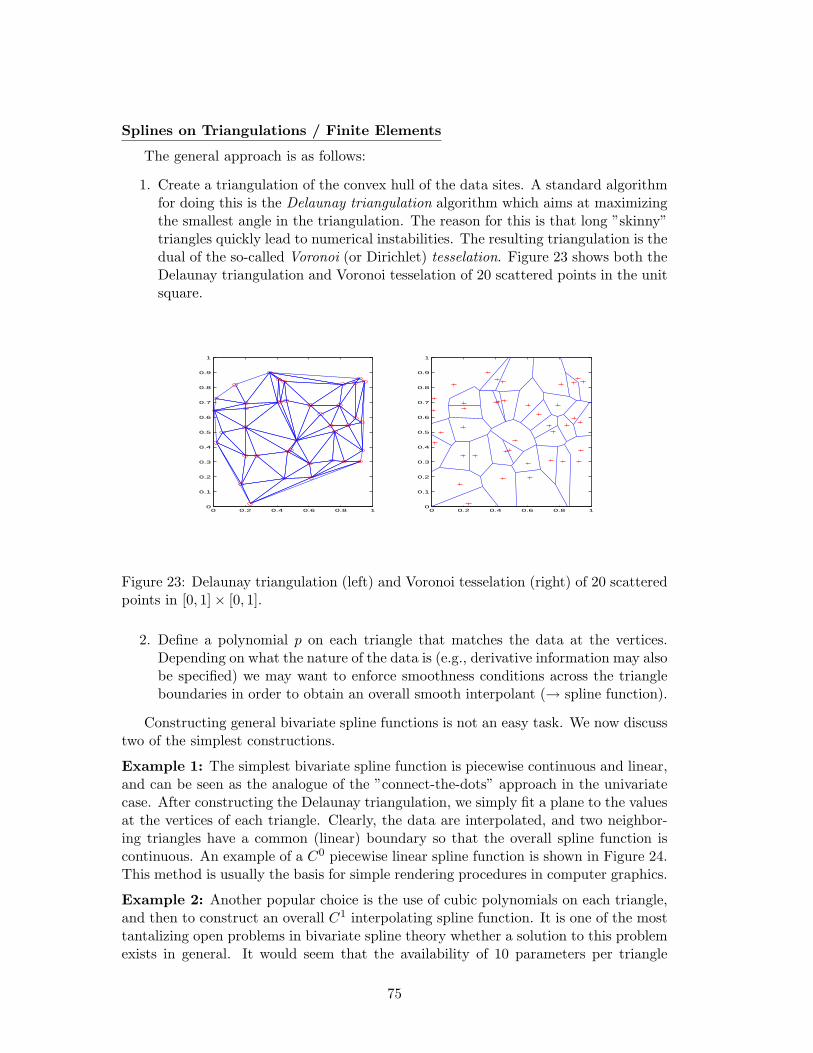
Splines on Triangulations / Finite Elements

The general approach is as follows:

1. Create a triangulation of the convex hull of the data sites. A standard algorithmfor doing this is the Delaunay triangulation algorithm which aims at maximizingthe smallest angle in the triangulation. The reason for this is that long ”skinny”triangles quickly lead to numerical instabilities. The resulting triangulation is thedual of the so-called Voronoi (or Dirichlet) tesselation. Figure 23 shows both theDelaunay triangulation and Voronoi tesselation of 20 scattered points in the unitsquare.

0 0.2 0.4 0.6 0.8 10

0.1

0.2

0.3

0.4

0.5

0.6

0.7

0.8

0.9

1

0 0.2 0.4 0.6 0.8 10

0.1

0.2

0.3

0.4

0.5

0.6

0.7

0.8

0.9

1

Figure 23: Delaunay triangulation (left) and Voronoi tesselation (right) of 20 scatteredpoints in [0, 1]× [0, 1].

2. Define a polynomial p on each triangle that matches the data at the vertices.Depending on what the nature of the data is (e.g., derivative information may alsobe specified) we may want to enforce smoothness conditions across the triangleboundaries in order to obtain an overall smooth interpolant (→ spline function).

Constructing general bivariate spline functions is not an easy task. We now discusstwo of the simplest constructions.

Example 1: The simplest bivariate spline function is piecewise continuous and linear,and can be seen as the analogue of the ”connect-the-dots” approach in the univariatecase. After constructing the Delaunay triangulation, we simply fit a plane to the valuesat the vertices of each triangle. Clearly, the data are interpolated, and two neighbor-ing triangles have a common (linear) boundary so that the overall spline function iscontinuous. An example of a C0 piecewise linear spline function is shown in Figure 24.This method is usually the basis for simple rendering procedures in computer graphics.

Example 2: Another popular choice is the use of cubic polynomials on each triangle,and then to construct an overall C1 interpolating spline function. It is one of the mosttantalizing open problems in bivariate spline theory whether a solution to this problemexists in general. It would seem that the availability of 10 parameters per triangle

75

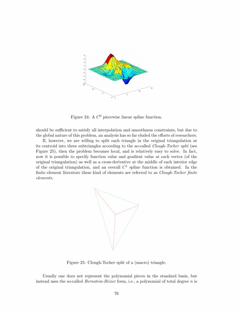
0

5

10

15

0

5

10

15−8

−6

−4

−2

0

2

4

6

8

Figure 24: A C0 piecewise linear spline function.

should be sufficient to satisfy all interpolation and smoothness constraints, but due tothe global nature of this problem, an analysis has so far eluded the efforts of researchers.

If, however, we are willing to split each triangle in the original triangulation atits centroid into three subtriangles according to the so-called Clough-Tocher split (seeFigure 25), then the problem becomes local, and is relatively easy to solve. In fact,now it is possible to specify function value and gradient value at each vertex (of theoriginal triangulation) as well as a cross-derivative at the middle of each interior edgeof the original triangulation, and an overall C1 spline function is obtained. In thefinite element literature these kind of elements are referred to as Clough-Tocher finiteelements.

Figure 25: Clough-Tocher split of a (macro) triangle.

Usually one does not represent the polynomial pieces in the standard basis, butinstead uses the so-called Bernstein-Bezier form, i.e., a polynomial of total degree n is

76

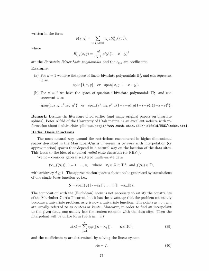
written in the formp(x, y) =

∑i+j+k=n

cijkBnijk(x, y),

whereBn

ijk(x, y) =n!

i!j!k!xiyj(1− x− y)k

are the Bernstein-Bezier basis polynomials, and the cijk are coefficients.

Example:

(a) For n = 1 we have the space of linear bivariate polynomials Π21, and can represent

it asspan1, x, y or spanx, y, 1− x− y.

(b) For n = 2 we have the space of quadratic bivariate polynomials Π22, and can

represent it as

span1, x, y, x2, xy, y2 or spanx2, xy, y2, x(1−x−y), y(1−x−y), (1−x−y)2.

Remark: Besides the literature cited earlier (and many original papers on bivariatesplines), Peter Alfeld of the University of Utah maintains an excellent website with in-formation about multivariate splines at http://www.math.utah.edu/∼alfeld/MDS/index.html.

Radial Basis Functions

The most natural way around the restrictions encountered in higher-dimensionalspaces described in the Mairhuber-Curtis Theorem, is to work with interpolation (orapproximation) spaces that depend in a natural way on the location of the data sites.This leads to the idea of so-called radial basis functions (or RBFs).

We now consider general scattered multivariate data

(xi, f(xi)), i = 1, . . . , n, where xi ∈ Ω ⊂ IRd, and f(xi) ∈ IR,

with arbitrary d ≥ 1. The approximation space is chosen to be generated by translationsof one single basic function ϕ, i.e.,

S = spanϕ(‖ · −z1‖), . . . , ϕ(‖ · −zm‖).

The composition with the (Euclidean) norm is not necessary to satisfy the constraintsof the Mairhuber-Curtis Theorem, but it has the advantage that the problem essentiallybecomes a univariate problem, as ϕ is now a univariate function. The points z1, . . . , zm,are usually referred to as centers or knots. Moreover, in order to find an interpolantto the given data, one usually lets the centers coincide with the data sites. Then theinterpolant will be of the form (with m = n)

s(x) =n∑

j=1

cjϕ(‖x− xj‖), x ∈ IRd, (39)

and the coefficients cj are determined by solving the linear system

Ac = f, (40)

77

that arises from the interpolation conditions

s(xi) = f(xi), i = 1, . . . , n.

Here the matrix A has entries ϕ(‖xi − xj‖).

Theorem 6.48 The interpolation matrix A in (40) is nonsingular for any set of dis-tinct data sites x1, . . . ,xn provided the d-variate function Φ defined by Φ(x) = ϕ(‖x‖)is strictly positive definite.

Proof: Next semester. ♠

In order to understand this theorem we need

Definition 6.49 A function f : IRd → IR is positive definite if for all n, all sets ofpairwise distinct x1, . . . ,xn ⊂ IRd, and all c ∈ IRn we have

n∑i=1

n∑j=1

cicjf(xi − xj) ≥ 0. (41)

If equality in (41) implies c1 = . . . = cn = 0, then f is called strictly positive definite.

Remarks:

1. The terminology in Definition 6.49 is somewhat ”nonstandard” as it does notmatch the one from linear algebra. However, positive definite functions werefirst defined in the 1920s by Bochner and others, and at that time there seemedto be no need for the ”strict” case. This part of the definition was only addedin the 1980s when Charles Micchelli discovered the connection between radialbasis functions and positive definite functions and proved (a stronger form of)Theorem 6.48.

2. The generalization of Theorem 6.48 involves so-called strictly conditionally posi-tive definite functions.

3. Of course, any kind of function ϕ that makes A nonsingular will work, but thecomplete characterization of such functions is still open.

Examples of RBFs

We use the abbreviation r = ‖x−xj‖. Then some of the most popular radial basicfunctions are:

1. Multiquadrics:ϕ(r) =

√r2 + α2, α > 0,

with parameter α. These functions have an associated function Φ that is strictlyconditionally negative definite of order one.

78

2. Inverse multiquadrics:

ϕ(r) =1√

r2 + α2, α > 0,

with parameter α. These functions give rise to strictly positive definite functions.

3. Gaussians:ϕ(r) = e−α2r2

, α > 0,

with parameter α. These functions give rise to strictly positive definite functions.

4. Thin plate splines (in IR2):ϕ(r) = r2 ln r.

These functions give rise to strictly conditionally positive definite functions oforder two.

5. Wendland’s compactly supported RBFs. There is a whole family of these func-tions. E.g.,

ϕ(r) = (1− r)4+(4r + 1)

gives rise to strictly positive definite functions as long as d ≤ 3.

To find a scattered data interpolant using RBFs one needs to solve the linear system(40). This system will be a dense system for RBFs 1–4, and sparse for those listed in5. Presently, one of the major research focusses is efficient solution of the system (40)and fast evaluation of the expansion (39).

Remarks:

1. The functions listed under 1–3 have spectral approximation order, i.e., they canapproximate a sufficiently smooth function arbitrarily closely. This approxima-tion is achieved by varying the parameter α. However, there is a trade-off principleinvolved, i.e., as the approximation quality is improved, the linear system (40)becomes more and more ill-conditioned.

2. RBF interpolation is illustrated in the Maple worksheet 578 RBF.mws.

Moving Least Squares Approximation

We begin by discussing discrete weighted least squares approximation from thespace of multivariate polynomials. Thus, we consider data

(xi, f(xi)), i = 1, . . . , n, where xi ∈ Ω ⊂ IRd, and f(xi) ∈ IR,

with arbitrary d ≥ 1. The approximation space is of the form

S = spanp1, . . . , pm, m < n,

with multivariate polynomials pm.

79

We intend to find the best discrete weighted least squares approximation from S tosome given function f , i.e., we need to determine the coefficients cj in

s(x) =m∑

j=1

cjpj(x), x ∈ IRd,

such that‖f − s‖2,w → min.

Here the norm is defined via the discrete (pseudo) inner product

〈f, g〉w =n∑

i=1

f(xi)g(xi)wi

with scalar weights wi, i = 1, . . . , n. The norm is then

‖f‖22,w =

n∑i=1

[f(xi)]2 wi.

From Section 6.8 we know that the best approximation s is characterized by

f − s ⊥ S ⇐⇒ 〈f − s, pk〉w = 0, k = 1, . . . ,m,

⇐⇒ 〈f −m∑

j=1

cjpj , pk〉w = 0

⇐⇒m∑

j=1

cj〈pj , pk〉w = 〈f, pk〉w, k = 1, . . . ,m.

These are of course the normal equations associated with this problem.

Now we discuss moving least squares approximation. The difference to the previouscase is that now the weights wi move with the evaluation point x, i.e., we have a newinner product

〈f, g〉w(x) =n∑

i=1

f(xi)g(xi)wi(x).

Therefore, the normal equations become

m∑j=1

cj〈pj , pk〉w(x) = 〈f, pk〉w(x), k = 1, . . . ,m.

Note that now the coefficients cj have an implicit dependence on the evaluation pointx. Therefore, the moving least squares best approximation from S is given by

s(x) =m∑

j=1

cj(x)pj(x).

Remark: This means that for every evaluation of s at a different point x the system ofnormal equations needs to be solved anew. This (seemingly) high computational cost

80

was one of the main reasons the moving least squares method was largely ignored afterit discovery in the early 1980s.

Example 1: We take S = span1 with d arbitrary. Then m = 1, and there is onlyone normal equation

c1〈p1, p1〉w(x) = 〈f, p1〉w(x)

which we can easily solve for the unknown expansion coefficient, so that

c1 =〈f, 1〉w(x)

〈1, 1〉w(x).

Thus,s(x) = c1(x)p1(x) = c1(x).

It is also easy to determine an explicit formula for c1(x). Since

〈f, 1〉w(x) =n∑

i=1

f(xi)1wi(x),

〈1, 1〉w(x) =n∑

i=1

1 · 1wi(x),

we have

s(x) = c1(x) =n∑

i=1

f(xi)wi(x)

n∑`=1

w`(x)

=n∑

i=1

f(xi)vi(x), (42)

wherevi(x) =

wi(x)n∑

`=1

w`(x).

This method is known as Shepard’s method (see Computer homework problem 6.10#1).

Remarks:

1. First, notice that the expansion (42) is an explicit formula for the best movingleast squares approximation – valid for any evaluation point x. Repeated solutionof the normal equations is not required, since we solved the one normal equationonce and for all analytically.

2. The functions vi, i = 1, . . . , n, can be seen as (approximate) cardinal basis func-tions. They are true cardinal functions if the weight functions are chosen ap-propriately (see the remarks regarding the choice of weight functions below).Expansion (42) can be viewed as a quasi-interpolation formula for the data givenby the function f .

81

3. Note that the functions vi, i = 1, . . . , n, form a partition of unity, i.e.,

n∑i=1

vi(x) = 1, x ∈ IRd .

Therefore, if the data comes from a constant function, i.e., f(xi) = C, then

s(x) =n∑

i=1

f(xi)vi(x) = Cn∑

i=1

vi(x) = C,

and Shepard’s method reproduces constants. This can be used to show that,if h denotes the ”meshsize” of the scattered data, then Shepard’s method hasapproximation order O(h).

4. By reproducing higher-degree polynomials (and thus solving non-trivial systemsof normal equations) one can achieve higher order of approximation with themoving least squares method.

5. We emphasize that the moving least squares method in general does not producea function that interpolates the given data – only an approximation.

6. The moving least squares method can be generalized by choosing a differentapproximation space S.

7. The smoothness of the overall approximation is governed by the smoothness ofthe functions in S as well as the smoothness of the weight functions.

Example 2:

If we take S = span1, x with d = 1, then m = 2, and the system of normalequations is

2∑j=1

cj〈pj , pk〉w(x) = 〈f, pk〉w(x), k = 1, 2,

or [〈p1, p1〉w(x) 〈p2, p1〉w(x)

〈p1, p2〉w(x) 〈p2, p2〉w(x)

] [c1

c2

]=

[〈f, p1〉w(x)

〈f, p2〉w(x)

]

⇐⇒

n∑

i=1

wi(x)n∑

i=1

xiwi(x)

n∑i=1

xiwi(x)n∑

i=1

x2i wi(x)

[

c1

c2

]=

n∑

i=1

f(xi)wi(x)

n∑i=1

f(xi)xiwi(x)

.

As mentioned above, this system has to be solved for every evaluation at a differentvalue x. For a fixed value x we have

s(x) =2∑

j=1

cj(x)pj(x) = c1(x) + xc2(x). (43)

82

Remarks:

1. We can see that (43) represents the equation of a line. However, depending onthe point of evaluation, a different line is chosen.

2. In the statistics literature this idea is known as local polynomial regression.

Choice of Weight Functions

1. In the early discussions of the moving least squares method (in the early 1980s byLancaster & Salkauskas) so-called inverse distance weight functions of the form

wi(x) = ‖x− xi‖−α, α > 0,

were suggested. Note that wi(x) → ∞ as x → xi. Therefore, using this kind ofweight function leads to interpolation of the given data.

2. The RBFs of the previous section can be used as weight functions.

3. B-splines (composed with the Euclidean norm if d > 1) have also been suggestedas (radial) weight functions.

4. Recent work by Fasshauer suggests that certain polynomials with a radial ar-gument can be used to construct Shepard-like functions with arbitrarily highapproximation orders.

Remark: If n is large, then it is more efficient to have local weight functions since not

all terms inn∑

i=1

. . . wi(x) coming from the inner product will be ”active” – only those

for which xi is close to x.

83