incorporating adjustments for the nonresponse and poststratification. But such

weights usually are not included in many survey data sets, nor is there the

appropriate information for creating such replicate weights.

Searching for Appropriate Models for Survey Data Analysis*

It has been said that many statistical analyses are carried out with no clear

idea of the objective. Before analyzing the data, it is essential to think

around the research question and formulate a clear analytic plan. As discussed

in a previous section, a preliminary analysis and exploration of data are very

important in survey analysis. In a model-based analysis, this task is much

more formidable than in a design-based analysis.

Problem formulation may involve asking questions or carrying out appro-

priate background research in order to get the necessary information for

choosing an appropriate model. Survey analysts often are not involved in col-

lecting the survey data, and it is often difficult to comprehend the data collec-

tion design. Asking questions about the initial design may not be sufficient, but

it is necessary to ask questions about how the design was executed in the field.

Often, relevant design-related information is neither documented nor included

in the data set. Moreover, some surveys have overly ambitious objectives

given the possible sample size. So-called general purpose surveys cannot pos-

sibly include all the questions that are relevant to all future analysts. Building

an appropriate model including all the relevant variables is a real challenge.

There should also be a check on any prior knowledge, particularly when

similar sets of data have been analyzed before. It is advisable not to fit a

model from scratch but to see if the new data are compatible with earlier

results. Unfortunately, it is not easy to find model-based analyses using com-

plex survey data in social and health science research. Many articles dealing

with the model-based analysis tend to concentrate on optimal procedures for

analyzing survey data under somewhat idealized conditions. For example,

most public use survey data sets contain only strata and PSUs, and opportu-

nities for defining additional target parameters for multilevel or hierarchical

linear models (Bryk & Raudenbush, 1992; Goldstein & Silver, 1989; Korn &

Graubard, 2003) are limited. The use of mixed linear models for complex

survey data analysis would require further research and, we hope, stimulate

survey designers to bring design and analysis into closer alignment.

6. CONDUCTING SURVEY DATA ANALYSIS

This chapter presents various illustrations of survey data analysis. The

emphasis is on the demonstration of the effects of incorporating the weights

and the data structure on the analysis. We begin with a strategy for conducting

49

a preliminary analysis of a large-scale, complex survey. Data from Phase II of

NHANES III (refer to Note 4) will be used to illustrate various analyses,

including descriptive analysis, linear regression analysis, contingency table

analysis, and logistic regression analyses. For each analysis, some theoretical

and practical considerations required for the survey data will be discussed.

The variables used in each analysis are selected to illustrate the methods

rather than to present substantive findings. Finally, the model-based perspec-

tive is discussed as it relates to analytic examples presented in this chapter.

A Strategy for Conducting Preliminary Analysis

Sample weights can play havoc in the preliminary analysis of complex

survey data, but exploring the data ignoring the weights is not a satisfactory

solution. On the other hand, programs for survey data analysis are not well

suited for basic data exploration. In particular, graphic methods were

not designed with complex surveys in mind. In this section, we present a

strategy for conducting preliminary analyses taking the weights into account.

Prior to the advent of the computer, the weight was handled in various ways

in data analysis. When IBM sorting machines were used for data tabulations,

it was common practice to duplicate the data cards to match the weight value

to obtain reasonable estimates. To expedite the tabulations of large-scale sur-

veys, the PPS procedure was adopted in some surveys (Murthy & Sethi,

1965). Recognizing the difficulty of analyzing complex survey data, Hinkins,

Oh, and Scheuren (1994) advocated an ‘‘inverse sampling design algorithm’’

that would generate a simple random subsample from the existing complex

survey data, so that users could apply their conventional statistical methods

directly to the subsample. These approaches are no longer attractive to survey

data analysis because programs for survey analysis are now readily available.

However, because there is no need to use entire data file for preliminary

analysis, the idea of subsampling by the PPS procedure is a very attractive

solution for developing data for preliminary analysis.

The PPS subsample can be explored by the regular descriptive and graphic

methods, because the weights are already reflected in the selection of the sub-

sample. For example, the scatterplot is one of the essential graphic methods

for preliminary data exploration. One way to incorporate the weight in the

scatterplot is the use of bubbles that represent the magnitude of the weight.

Recently, Korn and Graubard (1998) examined alternative procedures to

scatterplot bivariate data and showed advantages of using the PPS subsam-

ple. In fact, they found that ‘‘sampled scatterplots’’ are a preferred procedure

to ‘‘bubble scatterplots.’’

For a preliminary analysis, we generated a PPS sample of 1,000 from the

adult file of Phase II (1991–1994) of NHANES III (refer to Note 4), which

50

consisted of 9,920 adults. We first sorted the total sample by stratum and PSU

and then selected a PPS subsample systematically using a skipping interval of

9.92 on the scale of cumulated relative weights. The sorting by stratum and

PSU preserved in essence the integrity of the original sample design.

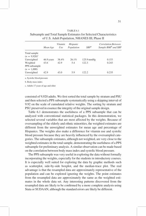
Table 6.1 demonstrates the usefulness of a PPS subsample that can be

analyzed with conventional statistical packages. In this demonstration, we

selected several variables that are most affected by the weights. Because of

oversampling of the elderly and ethnic minorities, the weighted estimates are

different from the unweighted estimates for mean age and percentage of

Hispanics. The weights also make a difference for vitamin use and systolic

blood pressure because they are heavily influenced by the oversampled cate-

gories. The subsample estimates, although not weighted, are very close to the

weighted estimates in the total sample, demonstrating the usefulness of a PPS

subsample for preliminary analysis. A similar observation can be made based

on the correlation between body mass index and systolic blood pressure.

The PPS subsample was very useful in exploring the data without formally

incorporating the weights, especially for the students in introductory courses.

It is especially well suited for exploring the data by graphic methods such

as scatterplot, side-by-side boxplot, and the median-trace plot. The real

advantage is that the resampled data are approximately representative of the

population and can be explored ignoring the weights. The point estimates

from the resampled data are approximately the same as the weighted esti-

mates in the whole data set. Any interesting patterns discovered from the

resampled data are likely to be confirmed by a more complete analysis using

Stata or SUDAAN, although the standard errors are likely be different.

TABLE 6.1

Subsample and Total Sample Estimates for Selected Characteristics

of U.S. Adult Population, NHANES III, Phase II

Mean Age

Vitamin

Use

Hispanic

Population SBPa

Correlation Between

Sample BMIb and SBP

Total sample

(n = 9,920)c

Unweighted 46.9 years 38.4% 26.1% 125.9 mmHg 0.153

Weighted 43.6 42.9 5.4 122.3 0.243

PPS subsample

(n = 1,000)

Unweighted 42.9 43.0 5.9 122.2 0.235

a. Systolic blood pressure

b. Body mass index

c. Adults 17 years of age and older

51

Conducting Descriptive Analysis

For a descriptive analysis, we used the adult sample (17 years of age or

older) from Phase II of NHANES III. It included 9,920 observations that

are arranged in 23 pseudo-strata, with 2 pseudo-PSUs in each stratum. The

identifications for the pseudo-strata (stra) and PSUs (psu) are included in

our working data file. The expansion weights in the data file were converted

to relative weights (wgt). To determine whether there were any problems in

the distribution of the observations across the PSUs, an unweighted tabula-

tion was performed. It showed that the numbers of observations available in

the PSUs ranged from 82 to 286. These PSU sample sizes seem sufficiently

large for further analysis.

We chose to examine the body mass index (BMI), age, race, poverty

index, education, systolic blood pressure, use of vitamin supplements, and

smoking status. BMI was calculated by dividing the body weight (in kilo-

grams) by the square of the height (in meters). Age was measured in years,

education (educat) was measured as the number of years of schooling, the

poverty index (pir) was calculated as a ratio of the family income to the

poverty level, and systolic blood pressure (sbp) was measured in mmHg.

In addition, the following binary variables are selected: Black (1 = black;

0 = nonblack), Hispanic (1 = Hispanic; 0 = non-Hispanic), use of vita-

min supplements (vituse) (1 = yes; 0 = no), and smoking status (smoker)

(1 = ever smoked; 0 = never smoked).

We imputed missing values for the variables selected for this analysis to

illustrate the steps of survey data analysis. Various imputation methods have

been developed to compensate for missing survey data (Brick & Kalton,

1996; Heitjan, 1997; Horton & Lipsitz, 2001; Kalton & Kasprszky, 1986;

Little & Rubin, 2002; Nielsen, 2003; Zhang, 2003). Several software packages

are available (e.g., proc mi & proc mianalyze in SAS/STAT; SOLAS;

MICE; S-Plus Missing Data Library). There are many ways to apply them

to a specific data set. Choosing appropriate methods and their course of

application ultimately depend on the number of missing values, the

mechanism that led to missing values (ignorable or nonignorable), and the

pattern of missing values (monotone or general). It is tempting to apply

sophisticated statistical procedures, but that may do more harm than good.

It will be more helpful to look at concrete examples (Kalton & Kasprszky,

1986; Korn & Graubard, 1999, sec. 4.7 and chap. 9) rather than reading tech-

nical manuals. Detailed discussions of these issues are beyond the scope of

this book. The following brief description is for illustrative purposes only.

There were no missing values for age and ethnicity in our data. We first

imputed values for variables with the fewest missing values. There were

fewer than 10 missing values for vituse and smoker and about 1% of values

52

missing for educat and height. We used a hot deck5 procedure to impute

values for these four variables by selecting donor observations randomly with

probability proportional to the sample weights within 5-year age categories

by gender. The same donor was used to impute values when there were miss-

ing values in one or more variables for an observation. Regression

imputation was used for height (3.7% missing; 2.8% based on weight, age,

gender, and ethnicity, and 0.9%, based on age, gender, and ethnicity), weight

(2.8% missing, based on height, age, gender, and ethnicity), sbp (2.5% miss-

ing, based on height, weight, age, gender and ethnicity), and pir (10% miss-

ing, based on family size, educat, and ethnicity). About 0.5% of imputed pir

values were negative, and these were set to 0.001 (the smallest pir value in

the data). Parenthetically, we could have brought other anthropometric mea-

sures into the regression imputation, but our demonstration was based simply

on the variables selected for this analysis. Finally, the bmi values (5.5%

missing) were recalculated based on updated weight and height information.

To demonstrate that the sample weight and design effect make a difference,

the analysis was performed under three different options: (a) unweighted,

ignoring the data structure; (b) weighted, ignoring the data structure; and

(c) survey analysis, incorporating the weights and sampling features. The first

option assumes simple random sampling, and the second recognizes the

weight but ignores the design effect. The third option provides an appropriate

analysis for the given sample design.

First, we examined the weighted means and proportions and their standard

errors with and without the imputed values. The imputation had inconsequen-

tial impact on point estimates and a slight reduction in estimated standard

errors under the third analytic option. The weighted mean pir without

imputed values was 3.198 (standard error = 0.114) compared with 3.168

(s:e: = 0.108) with imputed values. For bmi, the weighted mean was 25.948

(s:e: = 0.122) without imputation and 25.940 (s:e: = 0.118) with imputa-

tion. For other variables, the point estimates and their standard errors were

identical to the third decimal point because there were so few missing values.

The estimated descriptive statistics (using imputed values) are shown

in Table 6.2. The calculation was performed using Stata. The unweighted

statistics in the top panel were produced by the nonsurvey commands

summarize for point estimates and ci for standard errors. The weighted

analysis (second option) in the top panel was obtained by the same nonsur-

vey command with the use of [w�wgt]. The third analysis, incorporating

the weights and the design features, is shown in the bottom panel. It was

conducted using svyset [pweight�wgt], strata (stra), and psu (psu) for

setting complex survey features and svymean for estimating the means or

proportions of specified variables.

53

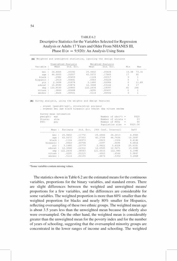
The statistics shown in Table 6.2 are the estimated means for the continuous

variables, proportions for the binary variables, and standard errors. There

are slight differences between the weighted and unweighted means/

proportions for a few variables, and the differences are considerable for

some variables. The weighted proportion is more than 60% smaller than the

weighted proportion for blacks and nearly 80% smaller for Hispanics,

reflecting oversampling of these two ethnic groups. The weighted mean age

is about 3.5 years less than the unweighted mean because the elderly also

were oversampled. On the other hand, the weighted mean is considerably

greater than the unweighted mean for the poverty index and for the number

of years of schooling, suggesting that the oversampled minority groups are

concentrated in the lower ranges of income and schooling. The weighted

(A) Weighted and unweighted statistics, ignoring the design features

Unweighted Analysis Weighted Analysis Variable | Mean Std. Err. Mean Std. Err. Min Max------------+---------------------------------------------------------------------- bmi | 26.4465 .05392 25.9402 .05428 10.98 73.16 age | 46.9005 .20557 43.5572 .17865 17 90 black | .2982 .00459 .1124 .00317 0 1 hispanic | .2614 .00441 .0543 .00228 0 1 pir | 2.3698 .01878 3.1680 .02086 0 11.89 educat | 10.8590 .03876 12.3068 .03162 0 17 sbp | 125.8530 .20883 122.2634 .18397 81 244 vituse | .3844 .00488 .4295 .00497 0 1 smoker | .4624 .00501 .5114 .00502 0 1-----------------------------------------------------------------------------------

(B) Survey analysis, using the weights and design features

. svyset [pweight=wgt], strata(stra) psu(psu)

. svymean bmi age black hispanic pir educat sbp vituse smoker

Survey mean estimationpweight: wgt Number of obs(*) = 9920Strata: stra Number of strata = 23PSU: psu Number of PSUs = 46 Population size = 9920.06------------------------------------------------------------------------ Mean | Estimate Std. Err. [95% Conf. Interval] Deff---------+-------------------------------------------------------------- bmi | 25.9402 .11772 25.6946 26.2013 4.9903 age | 43.5572 .57353 42.3708 44.7436 10.3067 black | .1124 .00973 .0923 .1326 9.4165 hispanic | .0543 .00708 .0397 .0690 9.6814 pir | 3.1680 .10779 2.9622 3.4328 25.6331 educat | 12.3068 .12312 12.0565 12.5671 15.0083 sbp | 122.2634 .38543 121.4010 122.980 4.1995 vituse | .4295 .01215 .4043 .4546 5.9847 smoker | .5114 .01155 .4874 .5352 5.2829------------------------------------------------------------------------

TABLE 6.2

Descriptive Statistics for the Variables Selected for Regression

Analysis or Adults 17 Years and Older From NHANES III,

Phase II (n = 9,920): An Analysis Using Stata

*Some variables contain missing values.

54

estimate for vitamin use is also somewhat greater than the unweighted

estimate. This lower estimate may reflect a lower use by minority groups.

The bottom panel presents the survey estimates that reflect both the

weights and design features. Although the estimated means and proportions

are exactly same as the weighed statistics in the top panel, the standard errors

increased substantially for all variables. This difference is reflected in the

design effect in the table (the square of the ratio of standard error in the

bottom panel to that for the weighted statistic in the top panel). The large

design effects for poverty index, education, and age partially reflect the resi-

dential homogeneity with respect to these characteristics. The design effects

of these socioeconomic variables and age are larger than those for the pro-

portion of blacks and Hispanics. The opposite was true in the NHANES II

conducted in late 1976–1980 (data presented in the first edition of this

book), suggesting that residential areas now increasingly becoming more

homogeneous with respect to socioeconomic status than by ethnic status.

The bottom panel also shows the 95% confidence intervals for the means

and proportions. The t value used for the confidence limits is not the familiar

value of 1.96 that might be expected from the sample of 9,920 (the sum of the

relative weights). The reason for this is that in a multistage cluster sampling

design, the degrees of freedom are based on the number of PSUs and strata,

rather than the sample size, as in SRS. Typically, the degrees of freedom in

complex surveys are determined as the number of PSUs sampled minus the

number of strata used. In our example, the degrees of freedom are 23

(= 46− 23) and t23, 0:975 = 2.0687; and this t value is used in all confidence

intervals in Table 6.2. In certain circumstances, the degrees of freedom may

be determined somewhat differently from the above general rule (see Korn &

Graubard, 1999, sec. 5.2).

In Table 6.3, we illustrate examples of conducting subgroup analysis. As

mentioned in the previous chapter, any subgroup analysis using complex

survey data should be done using the entire data set without selecting out

the data in the analytic domain. There are two options for conducting proper

subgroup analysis in Stata: the use of by or subpop. Examples of conduct-

ing a subgroup analysis for blacks are shown in Table 6.3. In the top panel,

the mean BMI is estimated separately for nonblacks and Blacks by using

the by option. The mean BMI for blacks is greater than for nonblacks.

Although the design effect of BMI among nonblacks (5.5) is similar to the

overall design effect (5.0 in Table 6.2), it is only 1.1 among blacks.

Stata also can be used to test linear combinations of parameters. The

equality of the two population subgroup means can be tested using the

lincom command ([bmi]1—[bmi]0, testing the hypothesis of the difference

between the population mean BMI for black = 1 and the mean BMI for

nonblack = 0), and the difference is statistically significant based on the

55

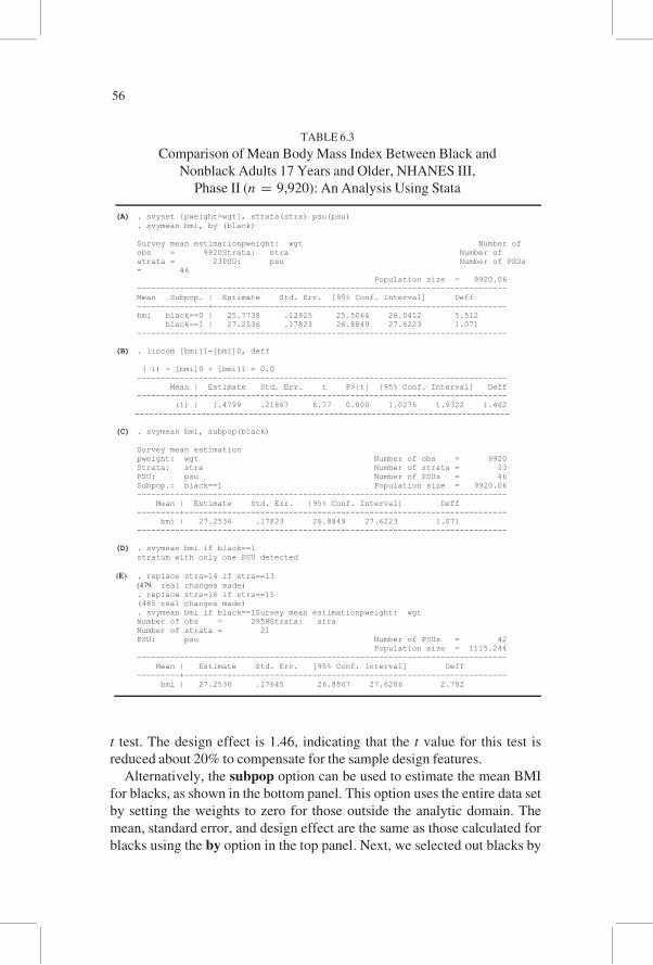
t test. The design effect is 1.46, indicating that the t value for this test is

reduced about 20% to compensate for the sample design features.

Alternatively, the subpop option can be used to estimate the mean BMI

for blacks, as shown in the bottom panel. This option uses the entire data set

by setting the weights to zero for those outside the analytic domain. The

mean, standard error, and design effect are the same as those calculated for

blacks using the by option in the top panel. Next, we selected out blacks by

(A) . svyset [pweight=wgt], strata(stra) psu(psu) . svymean bmi, by (black) Survey mean estimationpweight: wgt Number of obs = 9920Strata: stra Number of strata = 23PSU: psu Number of PSUs = 46 Population size = 9920.06 ------------------------------------------------------------------------------ Mean Subpop. | Estimate Std. Err. [95% Conf. Interval] Deff ---------------+-------------------------------------------------------------- bmi black==0 | 25.7738 .12925 25.5064 26.0412 5.512 black==1 | 27.2536 .17823 26.8849 27.6223 1.071 ------------------------------------------------------------------------------

(B) . lincom [bmi]1-[bmi]0, deff ( 1) - [bmi]0 + [bmi]1 = 0.0 ------------------------------------------------------------------------------ Mean | Estimate Std. Err. t P>|t| [95% Conf. Interval] Deff ------------+----------------------------------------------------------------- (1) | 1.4799 .21867 6.77 0.000 1.0275 1.9322 1.462

-------------------------------------------------------------------------------

(C) . svymean bmi, subpop(black)

Survey mean estimation pweight: wgt Number of obs = 9920 Strata: stra Number of strata = 23 PSU: psu Number of PSUs = 46 Subpop.: black==1 Population size = 9920.06 ------------------------------------------------------------------------------ Mean | Estimate Std. Err. [95% Conf. Interval] Deff ---------+-------------------------------------------------------------------- bmi | 27.2536 .17823 26.8849 27.6223 1.071 ------------------------------------------------------------------------------

(D) . svymean bmi if black==1 stratum with only one PSU detected

(E) . replace stra=14 if stra==13

(479 real changes made) . replace stra=16 if stra==15 (485 real changes made) . svymean bmi if black==1Survey mean estimationpweight: wgt Number of obs = 2958Strata: stra Number of strata = 21 PSU: psu Number of PSUs = 42 Population size = 1115.244 ------------------------------------------------------------------------------ Mean | Estimate Std. Err. [95% Conf. Interval] Deff ---------+--------------------------------------------------------------------

bmi | 27.2536 .17645 26.8867 27.6206 2.782

TABLE 6.3

Comparison of Mean Body Mass Index Between Black and

Nonblack Adults 17 Years and Older, NHANES III,

Phase II (n = 9,920): An Analysis Using Stata

56

specifying the domain (if black = = 1) to estimate the mean BMI. This

approach did not work because there were no blacks in some of the PSUs.

The tabulation of blacks by stratum and PSU showed that only one PSU

remained in the 13th and 15th strata. When these two strata are collapsed

with adjacent strata, Stata produced a result. Although the point estimate is

the same as before, the standard error and design effect are different. As a

general rule, subgroup analysis with survey data should avoid selecting out

a subset, unlike in the analysis of SRS data.

Besides the svymean command for descriptive analysis, Stata supports the

following descriptive analyses: svytotal (for the estimation of population

total), svyratio (for the ratio estimation), and svyprop (for the estimation of

proportions). In SUDAAN, these descriptive statistics can be estimated by

the DESCRIPT procedure, and subdomain analysis can be accommodated by

the use of the SUBPOPN statement.

Conducting Linear Regression Analysis

Both regression analysis and ANOVA examine the linear relation

between a continuous dependent variable and a set of independent vari-

ables. To test hypotheses, it is assumed that the dependent variable follows

a normal distribution. The following equation shows the type of relation

being considered by these methods for i = 1, 2, . . . , n:

Yi= β0 + β1X1i+β2X2i+ � � � + βpXpi+ εi (6:1)

This is a linear model in the sense that the dependent variable (Yi) is

represented by a linear combination of the βj’s plus εi: The βj is the coef-

ficient of the independent variable (Xj) in the equation, and εi is the ran-

dom error term in the model that is assumed to follow a normal distribution

with a mean of 0 and a constant variance and to be independent of the other

error terms.

In regression analysis, the independent variables are either continuous or

discrete variables, and the βj’s are the corresponding coefficients. In the

ANOVA, the independent variables (Xj’s) are indicator variables (under

effect coding, each category of a factor has a separate indicator variable

coded 1 or 0) that show which effects are added to the model, and the βj’s

are the effects.

Ordinary least squares (OLS) estimation is used to obtain estimates of the

regression coefficients or the effects in the linear model when the data result

from a SRS. However, several changes in the methodology are required to

deal with data from a complex sample. The data now consist of the individual

observations plus the sample weights and the design descriptors. As was

discussed in Chapter 3, the subjects from a complex sample usually have

57

different probabilities of selection. In addition, in a complex survey the

random error terms often are no longer independent of one another because

of features of the sample design. Because of these departures from SRS, the

OLS estimates of the model parameters and their variances are biased. Thus,

confidence intervals and tests of hypotheses may be misleading.

A number of authors have addressed these issues (Binder, 1983; Fuller,

1975; Holt, Smith, & Winter, 1980; Konijn, 1962; Nathan & Holt, 1980;

Pfeffermann & Nathan, 1981; Shah, Holt, & Folsom, 1977). They do not

concur on a single approach to the analysis, but they all agree that the use of

OLS as the estimation methodology can be inappropriate. Rather than

providing a review of all these works, we focus here on an approach that

covers the widest range of situations and that also has software available

and widely disseminated. This approach to the estimation of the model

parameters is the design-weighted least squares (DWLS), and its use is sup-

ported in SUDAAN, Stata, and other software for complex survey data

analysis.

The weight in the DWLS method is the sample weight discussed in

Chapter 3. DWLS is slightly different from the weighted least squares

(WLS) method for unequal variances, which derives the weight from an

assumed covariance structure (see Lohr, 1999, chap. 12). To account for the

complexities introduced by the sample design and other adjustments to the

weights, one of the methods discussed in Chapter 4 may be used in the esti-

mation of the variance-covariance matrix of the estimates of the model

parameters. Because these methods use the PSU total rather than the indivi-

dual value as the basis for the variance computation, the degrees of freedom

for this design equal the number of PSUs minus the number of strata,

instead of the sample size. The degrees of freedom associated with the sum

of squares for error are then the number of PSUsz minus the number of

strata, minus the number of terms in the model.

Table 6.4 presents the results of the multiple regression analysis of BMI on

the selected independent variables under the three options of analysis. For

independent variables, we used the same variables used for descriptive analy-

sis. In addition, age squared is included to account for a possible nonlinear

age effect on BMI. For simplicity, the interaction terms are not considered

in this example, although their inclusion undoubtedly would have increased

the R-squared, apart from a heightened multicollinearity problem. Imputed

values were used in this analysis. The regression coefficients were almost the

same as those obtained from the same analysis without using imputed values.

The standard errors of the coefficients were also similar between the analyses

with and without imputed values.

The top panel shows the results of unweighted and weighted analyses

ignoring the design features. The regress command is used for both the

58

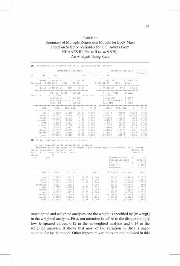
unweighted and weighted analyses and the weight is specified by [w�wgt]

in the weighted analysis. First, our attention is called to the disappointingly

low R-squared values, 0.12 in the unweighted analysis and 0.14 in the

weighted analysis. It shows that most of the variation in BMI is unac-

counted for by the model. Other important variables are not included in this

(A) Unweighted and weighted analysis, ignoring design features

Unweighted analysis Weighted analysis ------------------------------------------- ------------------------------------- Source | SS df MS | SS df MS ----------+------------------------------ -+------------------------------ Model | 33934.57 9 3770.48 | 37811.46 9 4201.27 Residual | 252106.39 9910 25.44 | 236212.35 9910 23.84 ----------+------------------------------ -+------------------------------ Total | 286040.68 9919 28.84 | 274023.81 9919 27.63 ----------------------------------------- -------------------------------- F( 9, 9910) = 148.21 F( 9, 9910) = 176.26 Prob > F = 0.0000 Prob > F = 0.0000 R-squared = 0.1186 R-squared = 0.1380 Adj R-squared = 0.1178 Adj R-squared = 0.1372

Root MSE = 5.0438 Root MSE = 4.8822 ------------------------------------------------ ------------------------------------- bmi | Coef. Std. Err. t P>|t| Coef. Std. Err. t P>|t| -----------+------------------------------------ ------------------------------------- age | .38422 .01462 26.27 0.000 .39778 .01528 26.03 0.000 agesq | -.00391 .00014 -27.61 0.000 -.00421 .00016 -27.06 0.000 black | 1.15938 .13178 8.80 0.000 .96291 .16108 5.98 0.000 hispanic | .70375 .14604 4.82 0.000 .64825 .22761 2.85 0.004 pir | -.14829 .03271 -4.53 0.000 -.12751 .02758 -4.62 0.000 educat | -.00913 .01680 -0.54 0.587 -.11120 .01865 -5.96 0.000 sbp | .05066 .00313 16.18 0.000 .07892 .00338 23.35 0.000 vituse | -.72097 .10752 -6.71 0.000 -.64256 .10176 -6.31 0.000 smoker | -.47851 .10456 -4.58 0.000 -.34981 .10033 -3.49 0.001 _cons | 12.70443 .49020 25.92 0.000 10.36452 .52213 19.85 0.000 ------------------------------------------------ ------------------------------------ (B) Survey analysis using the data features

. svyset [pweight=wgt], strata(stra) psu(psu) . svyregress bmi age agesq black hispanic pir educat sbp vituse smoker, deff Survey linear regression pweight: wgt Number of obs = 9920 Strata: stra Number of strata = 23 PSU: psu Number of PSUs = 46 Population size = 9920.06 F( 9, 15) = 71.84 Prob > F = 0.0000 R-squared = 0.1380 --------------------------------------------------------------------------------------- bmi | Coef. Std. Err. t P>|t| [95% Conf. Interval] Deff -----------+--------------------------------------------------------------------------- age | .39778 .02110 18.85 0.000 .35412 .44143 2.0539 agesq | -.00421 .00023 -18.02 0.000 -.00469 -.00373 2.3647 black | .96291 .22418 4.30 0.000 .49916 1.42666 1.5778 hispanic | .64825 .20430 3.17 0.004 .22562 1.07087 .8897 pir | -.12751 .05624 -2.27 0.033 -.24855 -.01117 4.5323 educat | -.11203 .02703 -4.11 0.000 -.16712 -.05529 2.1457 sbp | .07892 .00514 15.35 0.000 .06828 .08956 1.8798 vituse | -.64256 .17793 -3.61 0.001 -1.01063 -.27449 3.0546 smoker | -.34982 .20405 -1.71 0.100 -.77192 .07229 4.0343 _cons | 10.36452 .80124 12.94 0.000 8.70704 12.02201 2.3041 ---------------------------------------------------------------------------------------

TABLE 6.4

Summary of Multiple Regression Models for Body Mass

Index on Selected Variables for U.S. Adults From

NHANES III, Phase II (n = 9,920):

An Analysis Using Stata

59

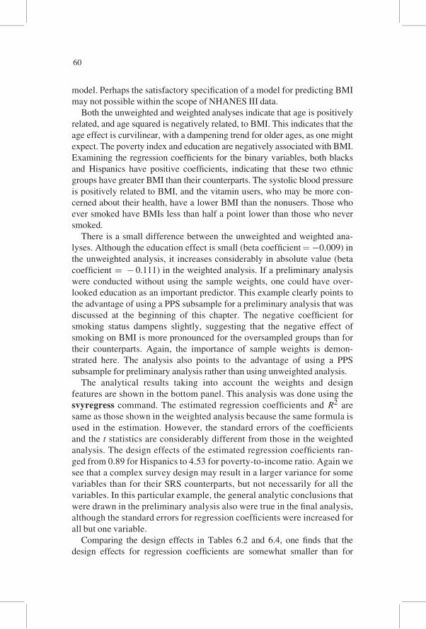
model. Perhaps the satisfactory specification of a model for predicting BMI

may not possible within the scope of NHANES III data.

Both the unweighted and weighted analyses indicate that age is positively

related, and age squared is negatively related, to BMI. This indicates that the

age effect is curvilinear, with a dampening trend for older ages, as one might

expect. The poverty index and education are negatively associated with BMI.

Examining the regression coefficients for the binary variables, both blacks

and Hispanics have positive coefficients, indicating that these two ethnic

groups have greater BMI than their counterparts. The systolic blood pressure

is positively related to BMI, and the vitamin users, who may be more con-

cerned about their health, have a lower BMI than the nonusers. Those who

ever smoked have BMIs less than half a point lower than those who never

smoked.

There is a small difference between the unweighted and weighted ana-

lyses. Although the education effect is small (beta coefficient¼−0.009) in

the unweighted analysis, it increases considerably in absolute value (beta

coefficient = − 0.111) in the weighted analysis. If a preliminary analysis

were conducted without using the sample weights, one could have over-

looked education as an important predictor. This example clearly points to

the advantage of using a PPS subsample for a preliminary analysis that was

discussed at the beginning of this chapter. The negative coefficient for

smoking status dampens slightly, suggesting that the negative effect of

smoking on BMI is more pronounced for the oversampled groups than for

their counterparts. Again, the importance of sample weights is demon-

strated here. The analysis also points to the advantage of using a PPS

subsample for preliminary analysis rather than using unweighted analysis.

The analytical results taking into account the weights and design

features are shown in the bottom panel. This analysis was done using the

svyregress command. The estimated regression coefficients and R2 are

same as those shown in the weighted analysis because the same formula is

used in the estimation. However, the standard errors of the coefficients

and the t statistics are considerably different from those in the weighted

analysis. The design effects of the estimated regression coefficients ran-

ged from 0.89 for Hispanics to 4.53 for poverty-to-income ratio. Again we

see that a complex survey design may result in a larger variance for some

variables than for their SRS counterparts, but not necessarily for all the

variables. In this particular example, the general analytic conclusions that

were drawn in the preliminary analysis also were true in the final analysis,

although the standard errors for regression coefficients were increased for

all but one variable.

Comparing the design effects in Tables 6.2 and 6.4, one finds that the

design effects for regression coefficients are somewhat smaller than for

60

the means and proportions. So, applying the design effect estimated from the

means and totals to regression coefficients (when the clustering information

is not available from the data) would lead to conclusions that are too conser-

vative. Smaller design effects may be possible in a regression analysis if the

regression model controls for some of the cluster-to-cluster variability. For

example, if part of the reason for people in the same cluster having similar

BMI is similar age and education, then one would expect that adjusting for

age and education in the regression model might account for some of cluster-

to-cluster variability. The clustering effect would then have less impact on

the residuals from the model.

Regression analysis can also be conducted by using the REGRESS

procedure in SUDAAN, as follows:

PROC REGRESS DESIGN = wr;

NEST stra psu;

WEIGHT wgt;

MODEL = bmi age agesq black hispanic pir educat sbs

vituse smoker;

RUN;

Conducting Contingency Table Analysis

The simplest form of studying the association of two discrete variables is

the two-way table. If data came from an SRS, we could use the Pearson chi-

square statistic to test the null hypothesis of independence. For the analysis of

a two-way table based on complex survey data, the test procedure needs to be

changed to account for the survey design. Several different test statistics have

been proposed. Koch, Freeman, and Freedman (1975) proposed using the

Wald statistic,6 and it has been used widely. The Wald statistic usually is

converted to an F statistic to determine the p value. In the F statistic, the

numerator degrees of freedom are tied to the dimension of the table, and the

denominator degrees of freedom reflect the survey design. Later, Rao and

Scott (1984) proposed correction procedures for the log-likelihood statistic,

using an F statistic with non-integer degrees of freedom. Based on a simula-

tion study (Sribney, 1998), Stata implemented the Rao-Scott corrected statis-

tic as the default procedure, but the Wald chi-square and the log- linear Wald

statistic are still available as option. On the other hand, SUDAAN uses the

Wald statistic in its CROSSTAB procedure. In most situations, these two

statistics lead to the same conclusion.

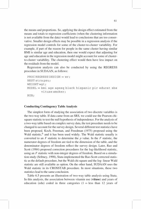
Table 6.5 presents an illustration of two-way table analysis using Stata.

In this analysis, the association between vitamin use (vituse) and years of

education (edu) coded in three categories (1 = less than 12 years of

61

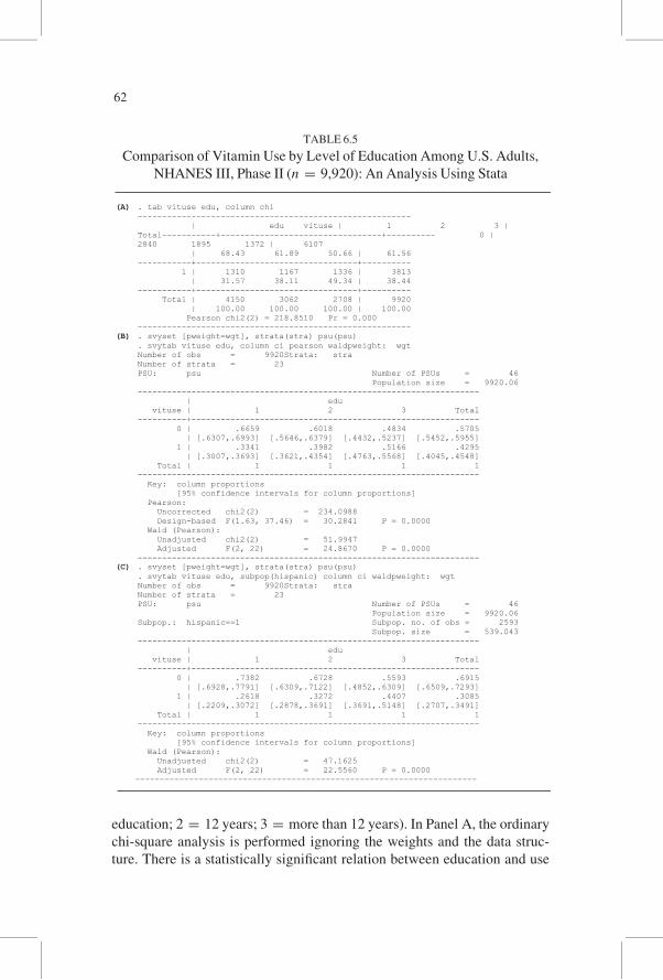
education; 2 = 12 years; 3 = more than 12 years). In Panel A, the ordinary

chi-square analysis is performed ignoring the weights and the data struc-

ture. There is a statistically significant relation between education and use

(A) . tab vituse edu, column chi -------------------------------------------------------- | edu vituse | 1 2 3 | Total-----------+---------------------------------+---------- 0 | 2840 1895 1372 | 6107 | 68.43 61.89 50.66 | 61.56 -----------+---------------------------------+---------- 1 | 1310 1167 1336 | 3813 | 31.57 38.11 49.34 | 38.44 -----------+---------------------------------+---------- Total | 4150 3062 2708 | 9920 | 100.00 100.00 100.00 | 100.00 Pearson chi2(2) = 218.8510 Pr = 0.000 --------------------------------------------------------

(B) . svyset [pweight=wgt], strata(stra) psu(psu) . svytab vituse edu, column ci pearson waldpweight: wgt Number of obs = 9920Strata: stra Number of strata = 23 PSU: psu Number of PSUs = 46 Population size = 9920.06 ---------------------------------------------------------------------- | edu vituse | 1 2 3 Total ----------+----------------------------------------------------------- 0 | .6659 .6018 .4834 .5705 | [.6307,.6993] [.5646,.6379] [.4432,.5237] [.5452,.5955] 1 | .3341 .3982 .5166 .4295 | [.3007,.3693] [.3621,.4354] [.4763,.5568] [.4045,.4548] Total | 1 1 1 1 ---------------------------------------------------------------------- Key: column proportions [95% confidence intervals for column proportions] Pearson: Uncorrected chi2(2) = 234.0988 Design-based F(1.63, 37.46) = 30.2841 P = 0.0000 Wald (Pearson): Unadjusted chi2(2) = 51.9947 Adjusted F(2, 22) = 24.8670 P = 0.0000 ----------------------------------------------------------------------

(C) . svyset [pweight=wgt], strata(stra) psu(psu) . svytab vituse edu, subpop(hispanic) column ci waldpweight: wgt Number of obs = 9920Strata: stra Number of strata = 23 PSU: psu Number of PSUs = 46 Population size = 9920.06 Subpop.: hispanic==1 Subpop. no. of obs = 2593 Subpop. size = 539.043 ---------------------------------------------------------------------- | edu vituse | 1 2 3 Total ----------+----------------------------------------------------------- 0 | .7382 .6728 .5593 .6915 | [.6928,.7791] [.6309,.7122] [.4852,.6309] [.6509,.7293] 1 | .2618 .3272 .4407 .3085 | [.2209,.3072] [.2878,.3691] [.3691,.5148] [.2707,.3491] Total | 1 1 1 1 ---------------------------------------------------------------------- Key: column proportions [95% confidence intervals for column proportions] Wald (Pearson): Unadjusted chi2(2) = 47.1625 Adjusted F(2, 22) = 22.5560 P = 0.0000

----------------------------------------------------------------------

TABLE 6.5

Comparison of Vitamin Use by Level of Education Among U.S. Adults,

NHANES III, Phase II (n = 9,920): An Analysis Using Stata

62

of vitamins, with those having a higher education being more inclined to

use vitamins. The percentage of vitamin users varies from 32% in the

lowest level of education to 49% in the highest level. Panel B shows the ana-

lysis of the same data taking the survey design into account. The weighted

percentage of vitamin users by the level of education varies slightly more

than in the unweighted percentages, ranging from 33% in the first level of

education to 52% in the third level of education. Note that with the request

of ci, Stata can compute confidence intervals for the cell proportions.

In this analysis, both Pearson and Wald chi-square statistics are requested.

The uncorrected Pearson chi-square, based on the weighed frequencies, is

slightly larger than the chi-square value in Panel A, reflecting the slightly

greater variation in the weighted percentages. However, a proper p value

reflecting the complex design cannot be evaluated based on the uncorrected

Pearson chi-square statistic. A proper p value can be evaluated from the

design-based F statistic of 30.28 with 1.63 and 37.46 degrees of freedom,

which is based on the test procedure as a result of the Rao-Scott correction.

The unadjusted Wald chi-square test statistic is 51.99, but a proper p value

must be determined based on the adjusted F statistic. The denominator

degrees of freedom in both F statistics reflect the number of PSUs and strata

in the sample design. The adjusted F statistic is only slightly smaller than the

Rao-Scott F statistic. Either one of these test statistics would lead to the same

conclusion.

In Panel C, the subpopulation analysis is performed for the Hispanic

population. Note that the entire data file is used in this analysis. The analysis

is based on 2,593 observations, but it represents only 539 people when

the sample weights are considered. The proportion of vitamin users among

Hispanics (31%) is considerably lower than the overall proportion of vitamin

users (43%). Again, there is a statistically significant relation between educa-

tion and use of vitamins among Hispanics, as the adjusted F statistic indicates.

Let us now look at a three-way table. Using the NHANES III, Phase II

adult sample data, we will examine gender difference in vitamin use across

the levels of education. This will be a 2× 2× 3 table, and we can perform a

two-way table analysis at each level of education. Table 6.6 shows the ana-

lysis of three 2× 2 tables using SAS and SUDAAN. The analysis ignoring

the survey design is shown in the top panel of the table. At the lowest level

of education, the percentage of vitamin use for males is lower than for

females, and the chi-square statistic suggests the difference is statistically

significant. Another way of examining the association in a 2× 2 table is the

calculation of the odds ratio.

In this table, the odds of using vitamins for males is 0.358 [¼ 0.2634/

(1− 0.2634)], and for females it is 0.567 [¼ 0.3617/(1− 0.3617)]. The

ratio of male odds over female odds is 0.63 (¼ 0.358/0.567), indicating that

63

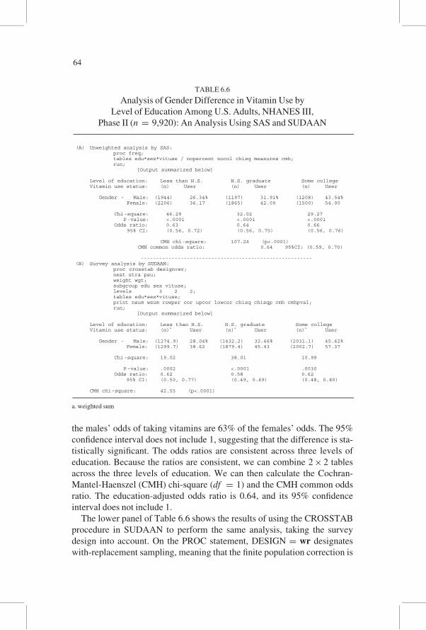
the males’ odds of taking vitamins are 63% of the females’ odds. The 95%

confidence interval does not include 1, suggesting that the difference is sta-

tistically significant. The odds ratios are consistent across three levels of

education. Because the ratios are consistent, we can combine 2× 2 tables

across the three levels of education. We can then calculate the Cochran-

Mantel-Haenszel (CMH) chi-square (df = 1) and the CMH common odds

ratio. The education-adjusted odds ratio is 0.64, and its 95% confidence

interval does not include 1.

The lower panel of Table 6.6 shows the results of using the CROSSTAB

procedure in SUDAAN to perform the same analysis, taking the survey

design into account. On the PROC statement, DESIGN = wr designates

with-replacement sampling, meaning that the finite population correction is

TABLE 6.6

Analysis of Gender Difference in Vitamin Use by

Level of Education Among U.S. Adults, NHANES III,

Phase II (n = 9,920): An Analysis Using SAS and SUDAAN

(A) Unweighted analysis by SAS: proc freq; tables edu*sex*vituse / nopercent nocol chisq measures cmh; run; [Output summarized below] Level of education: Less than H.S. H.S. graduate Some college Vitamin use status: (n) User (n) User (n) User Gender - Male: (1944) 26.34% (1197) 31.91% (1208) 43.54%

Female: (2206) 36.17 (1865) 42.09 (1500) 54.00 Chi-square: 46.29 32.02 29.27 P-value: <.0001 <.0001 <.0001 Odds ratio: 0.63 0.64 0.66 95% CI: (0.56, 0.72) (0.56, 0.75) (0.56, 0.76) CMH chi-square: 107.26 (p<.0001) CMH common odds ratio: 0.64 95%CI: (0.59, 0.70)

-------------------------------------------------------- (B) Survey analysis by SUDAAN:

proc crosstab design=wr; nest stra psu; weight wgt; subgroup edu sex vituse; levels 3 2 2; tables edu*sex*vituse; print nsum wsum rowper cor upcor lowcor chisq chisqp cmh cmhpval; run; [Output summarized below] Level of education: Less than H.S. H.S. graduate Some college Vitamin use status: (n)

a User (n)

a User (n)

a User

Gender - Male: (1274.9) 28.04% (1432.2) 32.66% (2031.1) 45.62% Female: (1299.7) 38.62 (1879.4) 45.43 (2002.7) 57.37 Chi-square: 19.02 38.01 10.99 P-value: .0002 <.0001 .0030 Odds ratio: 0.62 0.58 0.62 95% CI: (0.50, 0.77) (0.49, 0.69) (0.48, 0.80) CMH chi-square: 42.55 (p<.0001)

a. weighted sum

64

not used. The NEST statement designates the stratum and PSU variables.

The WEIGHT statement gives the weight variable. The SUBGROUP state-

ment declares three discrete variables, and the LEVELS statement specifies

the number of levels in each discrete variable. The TABLES statement

defines the form of contingency table. The PRINT statement requests nsum

(frequencies), wsum (weighted frequencies), rowper (row percent), cor

(crude odds ratio), upcor (upper limit of cor), lowcor (lower limit of cor),

chisq (chi-square statistic), chisqp (p value for chi-square statistic), cmh

(CMH statistic), and cmhpval (p value for CMH).

The weighted percentages of vitamin use are slightly different from the

unweighted percentages. The Wald chi-square values in three separate

analyses are smaller than the Pearson chi-square values in the upper panel

except for the middle level of education. Although the odds ratio

remained almost the same at the lower level of education, it decreased

somewhat at the middle and higher levels of education. The CROSSTAB

procedure in SUDAAN did not compute the common odds ratio, but it can

be obtained from a logistic regression analysis to be discussed in the next

section.

Conducting Logistic Regression Analysis

The linear regression analysis presented earlier may not be useful to

many social scientists because many of the variables in social science

research generally are measured in categories (nominal or ordinal). A number

of statistical methods are available for analyzing categorical data, ranging

from basic cross-tabulation analysis, shown in the previous section, to gener-

alized linear models with various link functions. As Knoke and Burke (1980)

observed, the modeling approach revolutionized contingency table analysis

in the social sciences, casting aside most of the older methods for deter-

mining relationships among variables measured at discrete levels. Two

approaches have been widely used by social scientists: log-linear models

using the maximum likelihood approach (Bishop et al.; Knoke & Burke,

1980; Swafford, 1980) and the weighted least square approach (Forthofer &

Lehnen, 1981; Grizzle, Starmer, & Koch, 1969). The use of these two meth-

ods for analyzing complex survey data was illustrated in the first edition of

this book. In these models, the cell proportions or functions of them (e.g., nat-

ural logarithm in the log-linear model) are expressed as a linear combination

of effects that make up the contingency table. Because these methods are

restricted to contingency tables, continuous independent variables cannot

be included in the analysis.

In the past decade, social scientists have begun to use logistic regression

analysis more frequently because of its ability to incorporate a larger

65

number of explanatory variables, including continuous variables (Aldrich

& Nelson, 1984; DeMaris, 1992; Hosmer & Lemeshow, 1989; Liao, 1994).

Logistic regression and other generalized linear models with different link

functions are now implemented in software packages for complex survey

data analysis. Survey analysts can choose the most appropriate model from

an array of models. The application of the logit model is illustrated below,

using Stata and SUDAAN.

The ordinary linear regression analysis represented by Equation 6.1

examines the relationship between a continuous dependent variable and

one or more independent variables. The logistic regression is a method to

examine the association of a categorical outcome with a number of inde-

pendent variables. The following equation shows the type of modeling a

binary outcome variable Y for i = 1, 2, . . . , n:

log[πi/(1−πi)]= β0 + β1x1i+ β2x2i+ � � � + βp−1xp−1, i: (6:2)

In Equation 6.2, πi is the probability that yi= 1. This is a generalized

linear model with a link function of the log odds or logit. Instead of least

square estimation, the maximum likelihood approach (see Eliason, 1993) is

used to estimate the parameters. Because the simultaneous equations to be

solved are nonlinear with respect to the parameters, iterative techniques are

used. Maximum likelihood theory also offers an estimator of the covariance

matrix of the estimated β’s, assuming individual observations are random

and independent.

Just as in the analysis of variance model, if a variable has l levels, we only

use l− 1 levels in the model. We shall measure the effects of the l− 1 levels

from the effect of the omitted or reference level of the variable. The esti-

mated β(β̂) is the difference in logit between the level in the model and the

omitted level, that is, the natural log of odds ratio of the level in the model

over the level omitted. Thus, taking eβ̂ gives the odds ratio adjusted for

other variables in the model. The results of logistic regression usually are

summarized and interpreted as odds ratios (see Liao, 1994, chap. 3).

With complex survey data, the maximum likelihood estimation needs to

be modified, because each observation has a sample weight. The maximum

likelihood solution incorporating the weights is generally known as pseudo

or weighted maximum likelihood estimation (Chambless & Boyle, 1985;

Roberts, Rao, & Kumar, 1987). Whereas the point estimates are calculated

by the pseudo likelihood procedure, the covariance matrix of the estimated

β̂’s is calculated by one of the methods discussed in Chapter 4. As discussed

earlier, the approximate degrees of freedom associated with this covariance

matrix are the number of PSUs minus the number of strata. Therefore, the

66

standard likelihood-ratio test for model fit should not be used with the

survey logistic regression analysis. Instead of the likelihood-ratio test,

the adjusted Wald test statistic is used.

The selection and inclusion of appropriate predictor variables for a logistic

regression model can be done similarly to the process for linear regression.

When analyzing a large survey data set, the preliminary analysis strategy

described in the earlier section is very useful in preparing for a logistic regres-

sion analysis.

To illustrate logistic regression analysis, the same data used in Table 6.6

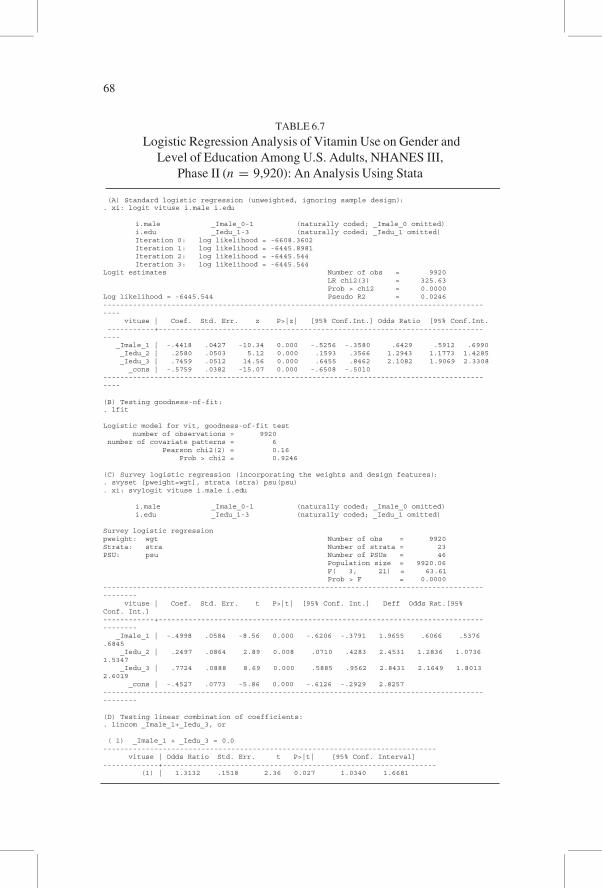
are analyzed using Stata. The analytical results are shown in Table 6.7. The

Stata output is edited somewhat to fit into a table. The outcome variable

is vitamin use (vituse), and explanatory variables are gender (1 = male;

0 = female) and level of education (edu). The interaction term is not

included in this model, based on the CMH statistic shown in Table 6.6.

First, we performed standard logistic regression analysis, ignoring the

weight and design features. The results are shown in Panel A. Stata automa-

tically performs the effect (or dummy) coding for discrete variables with

the use of the xi option preceding the logit statement and adding i. in front

of variable name.

The output shows the omitted level of each discrete variable. In this case,

the level ‘‘male’’ is in the model, and its effect is measured from the effect of

‘‘female,’’ the reference level. For education, being less than a high school

graduate is the reference level. The likelihood ratio chi-square value is 325.63

(df = 3) with p value of < 0.00001, and we reject the hypothesis that gender

and education together have no effect on vitamin usage, suggesting that there

is a significant effect. However, the pseudoR2 suggests that most of the varia-

tion in vitamin use is unaccounted for by these two variables. The parameter

estimates for gender and education and their estimated standard errors are

shown, as well as the corresponding test statistics. All factors are significant.

Including or in the model statement produces the odds ratios instead of

beta coefficients. The estimated odds ratio for males is 0.64, meaning that

the odds of taking vitamins for a male is 64% of the odds that a female uses

vitamins after adjusting for education. This odd ratio is the same as the

CMH common odds ratio shown in Table 6.6. The significance of the odds

ratio can be tested using either a z test or a confidence interval. The odds

ratio for the third level of education suggests that persons with some college

education are twice likely to take vitamins than those with less than

12 years of education, for the same gender. None of the confidence intervals

includes 1, suggesting that all effects are significant.

Panel B of Table 6.7 shows the goodness-of-fit statistic (chi-square with

df = 2). The large p value suggests that the main effects model fits the data

67

(A) Standard logistic regression (unweighted, ignoring sample design):. xi: logit vituse i.male i.edu

i.male _Imale_0-1 (naturally coded; _Imale_0 omitted)i.edu _Iedu_1-3 (naturally coded; _Iedu_1 omitted)Iteration 0: log likelihood = -6608.3602Iteration 1: log likelihood = -6445.8981Iteration 2: log likelihood = -6445.544Iteration 3: log likelihood = -6445.544

Logit estimates Number of obs = 9920 LR chi2(3) = 325.63 Prob > chi2 = 0.0000Log likelihood = -6445.544 Pseudo R2 = 0.0246--------------------------------------------------------------------------------------------- vituse | Coef. Std. Err. z P>|z| [95% Conf.Int.] Odds Ratio [95% Conf.Int. -----------+-------------------------------------------------------------------------------- _Imale_1 | -.4418 .0427 -10.34 0.000 -.5256 -.3580 .6429 .5912 .6990 _Iedu_2 | .2580 .0503 5.12 0.000 .1593 .3566 1.2943 1.1773 1.4285 _Iedu_3 | .7459 .0512 14.56 0.000 .6455 .8462 2.1082 1.9069 2.3308 _cons | -.5759 .0382 -15.07 0.000 -.6508 -.5010---------------------------------------------------------------------------------------------

(B) Testing goodness-of-fit:. lfit

Logistic model for vit, goodness-of-fit test number of observations = 9920 number of covariate patterns = 6 Pearson chi2(2) = 0.16 Prob > chi2 = 0.9246

(C) Survey logistic regression (incorporating the weights and design features):. svyset [pweight=wgt], strata (stra) psu(psu). xi: svylogit vituse i.male i.edu

i.male _Imale_0-1 (naturally coded; _Imale_0 omitted)i.edu _Iedu_1-3 (naturally coded; _Iedu_1 omitted)

Survey logistic regressionpweight: wgt Number of obs = 9920Strata: stra Number of strata = 23PSU: psu Number of PSUs = 46 Population size = 9920.06 F( 3, 21) = 63.61 Prob > F = 0.0000------------------------------------------------------------------------------------------------- vituse | Coef. Std. Err. t P>|t| [95% Conf. Int.] Deff Odds Rat.[95%Conf. Int.]------------+------------------------------------------------------------------------------------ _Imale_1 | -.4998 .0584 -8.56 0.000 -.6206 -.3791 1.9655 .6066 .5376.6845 _Iedu_2 | .2497 .0864 2.89 0.008 .0710 .4283 2.4531 1.2836 1.07361.5347 _Iedu_3 | .7724 .0888 8.69 0.000 .5885 .9562 2.8431 2.1649 1.80132.6019 _cons | -.4527 .0773 -5.86 0.000 -.6126 -.2929 2.8257-------------------------------------------------------------------------------------------------

(D) Testing linear combination of coefficients:. lincom _Imale_1+_Iedu_3, or

( 1) _Imale_1 + _Iedu_3 = 0.0------------------------------------------------------------------------------ vituse | Odds Ratio Std. Err. t P>|t| [95% Conf. Interval]-------------+---------------------------------------------------------------- (1) | 1.3132 .1518 2.36 0.027 1.0340 1.6681

TABLE 6.7

Logistic Regression Analysis of Vitamin Use on Gender and

Level of Education Among U.S. Adults, NHANES III,

Phase II (n = 9,920): An Analysis Using Stata

68

(not significantly different from the saturated model). In this simple situation,

the two degrees of freedom associated with the goodness of fit of the model

can also be interpreted as the two degrees of freedom associated with the

gender-by-education interaction. Hence, there is no interaction of gender and

education in relation to the proportion using vitamin supplements, confirming

the CMH analysis shown in Table 6.6.

Panel C of Table 6.7 shows the results of logistic regression analysis for

the same data, with the survey design taken into account. The log likelihood

is not shown because the pseudo likelihood is used. Instead of likelihood

ratio statistic, the F statistic is used. Again, the p value suggests that

the main effects model is a significant improvement over the null model.

The estimated parameters and odds ratios changed slightly because of the

sample weights, and the estimated standard errors of beta coefficients

increased, as reflected in the design effects. Despite the increased standard

errors, the beta coefficients for gender and education levels are significantly

different from 0. The odds ratio for males adjusted for education decreased

to 0.61 from 0.64. Although the odds ratio remained about the same for

the second level of education, its p value increased considerably, to 0.008

from< 0.0001, because of taking the design into account.

After the logistic regression model was run, the effect of linear combination

of parameters was tested as shown in Panel D. We wanted to test the hypoth-

esis that the sum of parameters for male and the third level of education is zero.

Because there is no interaction effect, the resulting odds ratio of 1.3 can be

interpreted as indicating that the odds of taking vitamin for males with some

college education are 30% higher than the odds for the reference (females with

less than 12 years of education). SUDAAN also can be used to perform a logis-

tic regression analysis, using its LOGISTIC procedure in the stand-alone ver-

sion or the RLOGIST procedure in the SAS callable version (a different name

used to distinguish it from the standard logistic procedure in SAS).

Finally, the logistic regression model also can be used to build a prediction

model for a synthetic estimation. Because most health surveys are designed to

estimate the national statistics, it is difficult to estimate health characteristics

for small areas. One approach to obtain estimates for small areas is the syn-

thetic estimation utilizing the national health survey and demographic infor-

mation of local areas. LaVange, Lafata, Koch, and Shah (1996) estimated the

prevalence of activity limitation among the elderly for U.S. states and counties

using a logistic regression model fit to the National Health Interview Survey

(NHIS) and Area Resource File (ARF). Because the NHIS is based on a com-

plex survey design, they used SUDAAN to fit a logistic regression model to

activity limitation indicators on the NHIS, supplemented with county-level

variables from ARF. The model-based predicted probabilities were then

extrapolated to calculate estimates of activity limitation for small areas.

69

Other Logistic Regression Models

The binary logistic regression model discussed above can be extended to

deal with more than two response categories. Some such response cate-

gories are ordinal, as in perceived health status: excellent, good, fair, and

poor. Other response categories may be nominal, as in religious prefer-

ences. These ordinal and nominal outcomes can be examined as function of

a set of discrete and continuous independent variables. Such modeling can

be applied to complex survey data, using Stata or SUDAAN. In this section,

we present two examples of such analyses without detailed discussion and

interpretation. For details of the models and their interpretation, see Liao

(1994).

To illustrate the ordered logistic regression model, we examined obesity

categories based on BMI. Public health nutritionists use the following criteria

to categorize BMI for levels of obesity: obese (BMI ≥ 30), overweight

(25≤BMI< 30), normal (18.5≤BMI< 25), and underweight (BMI< 18.5).

Based on NHANES III, Phase II data, 18% of U.S. adults are obese, 34%

overweight, 45% normal, and 3% underweight. We want to examine the rela-

tionship between four levels of obesity (bmi2: 1 = obese, 2 = overweight,

3 = normal, and 4 = underweight) and a set of explanatory variables includ-

ing age (continuous), education (edu), black, and Hispanic.

For the four ordered categories of obesity, the following three sets of

probabilities are modeled as functions of explanatory variables:

Prfobeseg versus Prfall other levelsgPrfobese plus overweightg versus Prfnormal plus underweightgPrfobese plus overweight plus normalg versus Prfunderweightg

Then three binary logistic regression models could be used to fit a separate

model to each of three comparisons. Recognizing the natural ordering of obe-

sity categories, however, we could estimate the ‘‘average’’ effect of explana-

tory variables by considering the three binary models simultaneously, based

on the proportional odds assumption. What is assumed here are that the

regression lines for the different outcome levels are parallel to each other and

that they are allowed to have different intercepts (this assumption needs to be

tested using the chi-square statistic; the test result is not shown in the table).

The following represents the model for j = 1, 2, . . . , c− 1 (c is the number

of categories in the dependent variable):

logPr(category≤j)

Pr(category≥ j+1ð Þ)

!

=αj +Xp

i=1

βixi (6:3)

From this model, we estimate (c− 1) intercepts and a set of β̂’s.

70

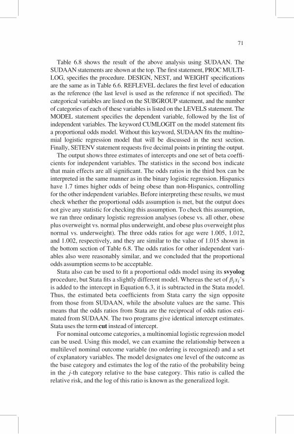
Table 6.8 shows the result of the above analysis using SUDAAN. The

SUDAAN statements are shown at the top. The first statement, PROC MULTI-

LOG, specifies the procedure. DESIGN, NEST, and WEIGHT specifications

are the same as in Table 6.6. REFLEVEL declares the first level of education

as the reference (the last level is used as the reference if not specified). The

categorical variables are listed on the SUBGROUP statement, and the number

of categories of each of these variables is listed on the LEVELS statement. The

MODEL statement specifies the dependent variable, followed by the list of

independent variables. The keyword CUMLOGIT on the model statement fits

a proportional odds model. Without this keyword, SUDAAN fits the multino-

mial logistic regression model that will be discussed in the next section.

Finally, SETENV statement requests five decimal points in printing the output.

The output shows three estimates of intercepts and one set of beta coeffi-

cients for independent variables. The statistics in the second box indicate

that main effects are all significant. The odds ratios in the third box can be

interpreted in the same manner as in the binary logistic regression. Hispanics

have 1.7 times higher odds of being obese than non-Hispanics, controlling

for the other independent variables. Before interpreting these results, we must

check whether the proportional odds assumption is met, but the output does

not give any statistic for checking this assumption. To check this assumption,

we ran three ordinary logistic regression analyses (obese vs. all other, obese

plus overweight vs. normal plus underweight, and obese plus overweight plus

normal vs. underweight). The three odds ratios for age were 1.005, 1.012,

and 1.002, respectively, and they are similar to the value of 1.015 shown in

the bottom section of Table 6.8. The odds ratios for other independent vari-

ables also were reasonably similar, and we concluded that the proportional

odds assumption seems to be acceptable.

Stata also can be used to fit a proportional odds model using its svyolog

procedure, but Stata fits a slightly different model. Whereas the set of βixi’s

is added to the intercept in Equation 6.3, it is subtracted in the Stata model.

Thus, the estimated beta coefficients from Stata carry the sign opposite

from those from SUDAAN, while the absolute values are the same. This

means that the odds ratios from Stata are the reciprocal of odds ratios esti-

mated from SUDAAN. The two programs give identical intercept estimates.

Stata uses the term cut instead of intercept.

For nominal outcome categories, a multinomial logistic regression model

can be used. Using this model, we can examine the relationship between a

multilevel nominal outcome variable (no ordering is recognized) and a set

of explanatory variables. The model designates one level of the outcome as

the base category and estimates the log of the ratio of the probability being

in the j-th category relative to the base category. This ratio is called the

relative risk, and the log of this ratio is known as the generalized logit.

71

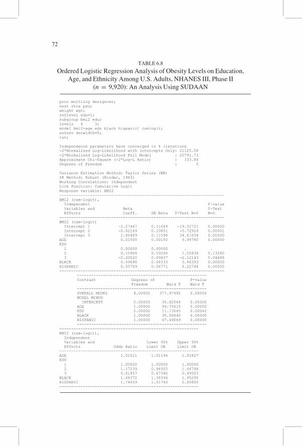
TABLE 6.8

Ordered Logistic Regression Analysis of Obesity Levels on Education,

Age, and Ethnicity Among U.S. Adults, NHANES III, Phase II

(n = 9,920): An Analysis Using SUDAAN

proc multilog design=wr; nest stra psu; weight wgt; reflevel edu=1; subgroup bmi2 edu; levels 4 3; model bmi2=age edu black hispanic/ cumlogit; setenv decwidth=5; run;

Independence parameters have converged in 4 iterations -2*Normalized Log-Likelihood with Intercepts Only: 21125.58 -2*Normalized Log-Likelihood Full Model : 20791.73 Approximate Chi-Square (-2*Log-L Ratio) : 333.86 Degrees of Freedom : 5 Variance Estimation Method: Taylor Series (WR) SE Method: Robust (Binder, 1983) Working Correlations: Independent Link Function: Cumulative Logit Response variable: BMI2 ---------------------------------------------------------------------- BMI2 (cum-logit), Independent P-value Variables and Beta T-Test Effects Coeff. SE Beta T-Test B=0 B=0 ---------------------------------------------------------------------- BMI2 (cum-logit) Intercept 1 -2.27467 0.11649 -19.52721 0.00000 Intercept 2 -0.62169 0.10851 -5.72914 0.00001 Intercept 3 2.85489 0.11598 24.61634 0.00000 AGE 0.01500 0.00150 9.98780 0.00000 EDU 1 0.00000 0.00000 . . 2 0.15904 0.10206 1.55836 0.13280 3 -0.20020 0.09437 -2.12143 0.04488 BLACK 0.49696 0.08333 5.96393 0.00000 HISPANIC 0.55709 0.06771 8.22744 0.00000 ----------------------------------------------------------------------

------------------------------------------------------- Contrast Degrees of P-value Freedom Wald F Wald F ------------------------------------------------------- OVERALL MODEL 8.00000 377.97992 0.00000 MODEL MINUS INTERCEPT 5.00000 36.82064 0.00000 AGE 1.00000 99.75615 0.00000 EDU 2.00000 11.13045 0.00042 BLACK 1.00000 35.56845 0.00000 HISPANIC 1.00000 67.69069 0.00000 -------------------------------------------------------

----------------------------------------------------------- BMI2 (cum-logit), Independent Variables and Lower 95% Upper 95% Effects Odds Ratio Limit OR Limit OR ----------------------------------------------------------- AGE 1.01511 1.01196 1.01827 EDU 1 1.00000 1.00000 1.00000 2 1.17239 0.94925 1.44798 3 0.81857 0.67340 0.99503 BLACK 1.64372 1.38346 1.95295 HISPANIC 1.74559 1.51743 2.00805 -----------------------------------------------------------

72

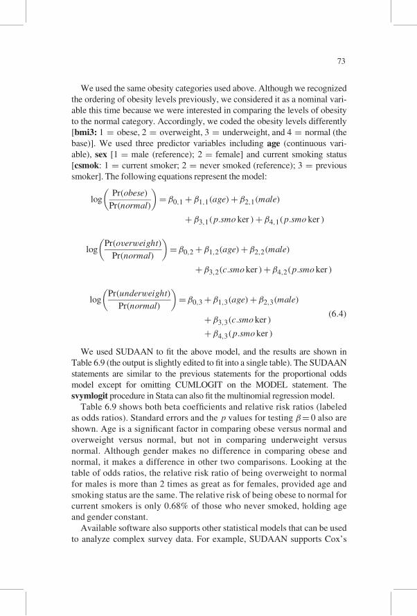
We used the same obesity categories used above. Although we recognized

the ordering of obesity levels previously, we considered it as a nominal vari-

able this time because we were interested in comparing the levels of obesity

to the normal category. Accordingly, we coded the obesity levels differently

[bmi3: 1 = obese, 2 = overweight, 3 = underweight, and 4 = normal (the

base)]. We used three predictor variables including age (continuous vari-

able), sex [1 = male (reference); 2 = female] and current smoking status

[csmok: 1 = current smoker; 2 = never smoked (reference); 3 = previous

smoker]. The following equations represent the model:

logPr(obese)

Pr(normal)

� �

= β0,1 + β1,1(age)+ β2,1(male)

+ β3,1(p:smo ker )+ β4,1(p:smo ker )

logPr(overweight)

Pr(normal)

� �

=β0,2 +β1,2(age)+β2,2(male)

+β3,2(c:smoker )+β4,2(p:smo ker )

logPr(underweight)

Pr(normal)

� �

=β0,3 +β1,3(age)+β2,3(male)

+β3,3(c:smoker )

+β4,3(p:smoker )

(6:4)

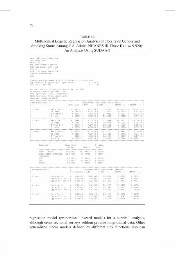
We used SUDAAN to fit the above model, and the results are shown in

Table 6.9 (the output is slightly edited to fit into a single table). The SUDAAN

statements are similar to the previous statements for the proportional odds

model except for omitting CUMLOGIT on the MODEL statement. The

svymlogit procedure in Stata can also fit the multinomial regression model.

Table 6.9 shows both beta coefficients and relative risk ratios (labeled

as odds ratios). Standard errors and the p values for testing β= 0 also are

shown. Age is a significant factor in comparing obese versus normal and

overweight versus normal, but not in comparing underweight versus

normal. Although gender makes no difference in comparing obese and

normal, it makes a difference in other two comparisons. Looking at the

table of odds ratios, the relative risk ratio of being overweight to normal

for males is more than 2 times as great as for females, provided age and

smoking status are the same. The relative risk of being obese to normal for

current smokers is only 0.68% of those who never smoked, holding age

and gender constant.

Available software also supports other statistical models that can be used

to analyze complex survey data. For example, SUDAAN supports Cox’s

73

regression model (proportional hazard model) for a survival analysis,

although cross-sectional surveys seldom provide longitudinal data. Other

generalized linear models defined by different link functions also can

TABLE 6.9

Multinomial Logistic Regression Analysis of Obesity on Gender and

Smoking Status Among U.S. Adults, NHANES III, Phase II (n = 9,920):

An Analysis Using SUDAAN

proc multilog design=wr; nest stra psu; weight wgt; reflevel csmok=2 sex=2; subgroup bmi2 csmok sex; levels 4 3 2; model bmi3=age sex csmok; setenv decwidth=5; run; Independence parameters have converged in 6 iterations Approximate ChiSquare (-2*Log-L Ration) : 587.42 Degrees of Freedom : 12 Variance Estimation Method: Taylor Series (WR) SE Method: Robust (Binder, 1983) Working Correlations: Independent Link Function: Generalized Logit Response variable: BMI3 ------------------------------------------------------------------------------------------------- | BMI3 log-odds)| | Independent Variables and Effects | | | | Intercept | AGE | SEX = 1 | CSMOK = 1 | CSMOK = 3 | ------------------------------------------------------------------------------------------------- | 1 vs 4 | Beta Coeff. | -1.33334 | 0.01380 | 0.08788 | -0.39015 | -0.27372 | | | SE Beta | 0.14439 | 0.00214 | 0.12509 | 0.07203 | 0.13206 | | | T-Test B=0 | -9.23436 | 6.43935 | 0.70251 | -5.41617 | 2.07277 | | | P-value | 0.00000 | 0.00000 | 0.48941 | 0.00002 | 0.04958 | ------------------------------------------------------------------------------------------------- | 2 vs 4 | Beta Coeff. | -1.25883 | 0.01527 | 0.76668 | -0.24271 | -0.02006 | | | SE Beta | 0.13437 | 0.00200 | 0.08275 | 0.11067 | 0.09403 | | | T-Test B=0 | -9.36835 | 7.64830 | 9.26512 | -2.19307 | -0.21335 | | | P-value | 0.00000 | 0.00000 | 0.00000 | 0.03868 | 0.83293 | ------------------------------------------------------------------------------------------------- | 3 vs 4 | Beta Coeff. | -2.07305 | -0.01090 | -1.16777 | 0.33434 | 0.04694 | | | SE Beta | 0.48136 | 0.00742 | 0.25280 | 0.30495 | 0.26168 | | | T-Test B=0 | -4.30663 | -1.46824 | -4.61937 | 1.09637 | 0.17936 | | | P-value | 0.00026 | 0.15558 | 0.00012 | 0.28427 | 0.85923| -------------------------------------------------------------------------------------------------

------------------------------------------------------- Contrast Degrees of P-value Freedom Wald F Wald F ------------------------------------------------------- OVERALL MODEL 15.00000 191.94379 0.00000 MODEL MINUS INTERCEP 12.00000 68.70758 0.00000 INTERCEPT . . . AGE 3.00000 22.97518 0.00000 SEX 3.00000 64.83438 0.00000 CSMOK 6.00000 6.08630 0.00063 -------------------------------------------------------

----------------------------------------------------------------------------------------------- | BMI3(log-odds)| | Independent Variables and Effects | | | | Intercept | AGE | SEX = 1 | CSMOK = 1 | CSMOK = 3 | ----------------------------------------------------------------------------------------------- | 1 vs 4 | Odds Ratio | 0.26360 | 1.01390 | 1.09186 | 0.67695 | 0.76054 | | | Lower 95% Limit | 0.19553 | 1.00941 | 0.84291 | 0.58323 | 0.57874 | | | Upper 95% Limit | 0.35535 | 1.01840 | 1.41433 | 0.78573 | 0.99946 | ----------------------------------------------------------------------------------------------- | 2 vs 4 | Odds Ratio | 0.28399 | 1.01539 | 2.15260 | 0.78450 | 0.98014 | | | Lower 95% Limit | 0.21507 | 1.01120 | 1.81393 | 0.62397 | 0.80689 | | | Upper 95% Limit | 0.37499 | 1.01959 | 2.55450 | 0.98633 | 1.19059 | ----------------------------------------------------------------------------------------------- | 3 vs 4 | Odds Ratio | 0.12580 | 0.98916 | 0.31106 | 1.39702 | 1.04805 | | | Lower 95% Limit | 0.04648 | 0.97408 | 0.18439 | 0.74341 | 0.60994 | | | Upper 95% Limit | 0.34052 | 1.00447 | 0.52476 | 2.62526 | 1.80086 | -----------------------------------------------------------------------------------------------

74

be applied to complex survey data, using the procedures supported by

SUDAAN, Stata, and other programs.

Design-Based and Model-Based Analysis*

All the analyses presented so far relied on the design-based approach, as

sample weights and design features were incorporated in the analysis.

Before relating these analyses to the model-based approach, let us briefly

consider the survey data used for these analyses. For NHANES III, 2,812

PSUs were formed, covering the United States. These PSUs consisted of

individual counties, but sometimes they included two or more adjacent

counties. These are administrative units, and the survey was not designed to

produce separate estimates for these units. From these units, 81 PSUs were

sampled, with selection probability proportional to the sizes of PSUs—13

from certainty strata and 2 from each of 34 strata formed according to these

demographic characteristics rather than geographic location. Again, strata

are not designed to define population parameters. The second stage of

sampling involved area segments consisting of city or suburban blocks or

other contiguous geographic areas. Segments with larger minority popula-

tion were sampled with a higher probability. The third stage of sampling

involved the listing of all the households within the sampled area segments

and then sampling them at a rate that depended on the segment characteris-

tics. The fourth stage of sampling was to sample individuals within sampled

households to be interviewed. These secondary units were used to facilitate

sampling rather than to define population parameters. The public-use data

file included only strata and PSUs; identification of seconding sampling

units was not included. Sample weights were calculated based on the selec-

tion probabilities of interviewed persons, with weighting adjustments for

nonresponse and poststratification. Many of the analytic issues discussed in

the previous chapters arise because of the way large-scale social and health

surveys are conducted. Available data are not prepared to support the use

of hierarchical linear models for incorporating the multistage selection

design.

Because of the unequal selection probabilities of interviewed indivi-

duals, coupled with adjustments for nonresponse and poststratification, it

is unconvincing to ignore the sample weights in descriptive analysis of

NHANES III data. The rationale for weighting in descriptive analysis has

been quite clear. As shown in Table 6.2, the bias in the unweighted estimate

is quite high for age and race-related variables. The standard error of the

weighted estimate is quite similar to that of the unweighted estimate for all

variables, suggesting that the variability in sample weights does not increase

the variance. However, the standard error for the weighted estimates taking

75

into account PSUs and strata is quite high, as reflected by the design effects.

One way to reduce the variance is the use of a model using auxiliary informa-

tion. Classical examples are the familiar ratio and regression estimators

(Cochran, 1977, chap. 6). In these estimators, the auxiliary information is in

the form of known population means of concomitant variables that are related

to the target variables. The use of auxiliary information can be extended to

the estimation of distribution functions (Rao, Kovar, & Mantel, 1990); how-

ever, the use of auxiliary information in routine descriptive analysis is limited

because finding suitable auxiliary information is difficult.

The use of a model in regression analysis is quite obvious. The

unweighted estimates in Table 6.4 are based strictly on a model-based

approach. It ignored the sample weights and the design features, but much

of the relevant design information is included among the independent vari-

ables, for example, age (oversampling of elderly persons) and black and

Hispanic (oversampling of minority populations). Indeed, the model-based

estimates of coefficients are similar to the weighted estimates, suggesting

that the model-based analysis is quite reasonable in this case. The one nota-

ble exception is the coefficient of education, which is very different under

the two estimation procedures. Education is highly insignificant in the

model-based analysis but highly significant in the weighted analysis. The

education effect could not be detected by the model-based analysis because

of the diminishing education effect for older ages. Age is included in the

model, but the interaction effect between age and education is not included

in the model. This example suggests that the use of the sample weights

protects against misspecification of the model.

Korn and Graubard (1995b) illustrate further the advantage of using

sample weights in a regression analysis, using data from the 1988 National

Maternal and Infant Health Survey. This survey oversampled low-

birthweight infants. The estimated regression lines of gestational age on

birthweight from the unweighted and weighted analysis turn out to be very

different. Although the unweighted fitting reflects sample observations

equally and does not describe the population, the weighted fitting pulls the

regression line to where the population is estimated to be. The relationship

between the two variables actually is curvilinear. If a quadratic regression

were fit instead, then the unweighted and weighted regressions would show

greater agreement.

As discussed above concerning the analytic results in Table 6.4, a careful

examination of the differences between the weighted and unweighted

regressions can sometimes identify important variables or interactions that

should be added to the model. The differences between the unweighted and

weighted estimates suggest that incorporating the sample design provides

protection against the possible misspecification of the population model.

76

Several statistics for testing the differences between the weighted and

unweighted estimates have been proposed in the literature (DuMouchel &

Duncan, 1983; Fuller, 1984; Nordberg, 1989). Korn and Graubard (1995a)

apply these test statistics to the NHANES I and II data using design-based

variances. They recommend the design-based analysis when the inefficiency

is small. Otherwise, additional modeling assumptions can be incorporated

into the analysis. They noted that secondary sampling units are not available

to the public and point to the need to increase the number of PSUs in the

design of large health surveys. These tests are limited to point estimation,

and therefore their conclusions may not apply to all circumstances. More

detailed discussion of these and related issues is provided by Pfeffermann

(1993, 1996).

The fact that the design-based analysis provides protection against possi-

ble misspecification of the model suggests that the analysis illustrated using

SUDAAN, Stata, other software for complex survey analysis is appropriate

for NHANES data. Even in the design-based analysis, a regression model is

used to specify the parameters of interest, but inference takes the sample

design into account. The design-based analysis in this case may be called

a model-assisted approach (Sarndal, Swensson, & Wretman, 1992). The

design-based theory relies on large sample sizes to make inferences about

the parameters. The model-based analysis may be a better option for a small

sample. When probability sampling is not used in data collection, there

is no basis for applying the design-based inference. The model-based

approach would make more sense where substantive theory and previous

empirical investigations support the proposed model.

The idea of model is less obvious in a contingency table analysis than in

a regression analysis. The rationale for design-based analysis taking into

account the sampling scheme already has been discussed. As in the regres-

sion analysis, it is wise to pay attention to the differences between the

weighted proportions and the unweighted proportions. If there is a sub-

stantial difference, one should explore why they differ. In Table 6.6, the

unweighted and weighted proportions are similar, but the weighted odds

ratios for vitamin use and gender are slightly lower than the unweighted

odds ratios for high school graduates and those with some college educa-

tion, while the weighted and unweighted odds ratios are about the same

for those with less than high school graduation. The small difference for

the two higher levels of education may be due to race or some other factor.

If the difference between the unweighted and weighted odds ratios is

much larger and it is due to race, one should examine the association sepa-

rately for different racial groups. The consideration of additional factors

in the contingency table analysis can be done using a logistic regression

model.

77

The uses of model and associated issues in a logistic regression are exactly

same as in a linear regression. A careful examination of the weighted and

unweighted analysis provides useful information. In Table 6.7, the weighted

and unweighted estimates of coefficients are similar. It appears that the

weighting affects the intercept more than the coefficients. The analysis shown

in Table 6.7 is a simple demonstration of analyzing data using logistic reg-

ression, and no careful consideration was given to choosing an appropriate

model. Comparable model-based analyses without using the weights and

sample design were not performed for the ordered logistic regression model

in Table 6.8 and multinomial logistic regression model in Table 6.9, because

we feel that an appropriate model including all relevant independent variables

is not specified.

In summary, analysis of complex survey data would require both the

model-based and design-based analysis. Design-based methods yield app-

roximately unbiased estimators or associations, but standard errors can be

ineffective. Model-based methods require assumptions in choosing the

model, and wrong assumptions can lead to biased estimators of associations

and standard errors.

7. CONCLUDING REMARKS

In this book, we have discussed the problematic aspects of survey data

analysis and methods for dealing with the problems caused by the use of

complex sample designs. The focus has been on understanding the problems

and the logic of the methods, rather than on providing a technical manual.

We also have presented a practical guide for preparing for an analysis of

complex survey data and demonstrated the use of some of the software avail-

able for performing various analyses. Software for complex survey analysis

is now readily available, and with the increasing computing power of perso-

nal computers, many sophisticated analytical methods can be implemented

easily. Nevertheless, data analysts need to specify the design, to create repli-

cate weights for certain analysis, and to choose appropriate test statistics for

survey analysis. Therefore, the user should have a good understanding of the

sample design and related analytical issues.

Although the material presented on these issues has been addressed

mainly to survey data analysts, we hope that this introduction also stimu-

lates survey designers and data producers to pay more attention to the needs

of the users of survey data. As more analytic uses are made of the survey

data that were initially collected for enumerative purposes, the survey

designers must consider including certain design-related information that

allow more appropriate analysis to be performed, as well as easing the

78