Embed Size (px)
Citation preview
5 Orbit and Ground Track of a Satellite
5.1 Position of the Satellite on its Orbit
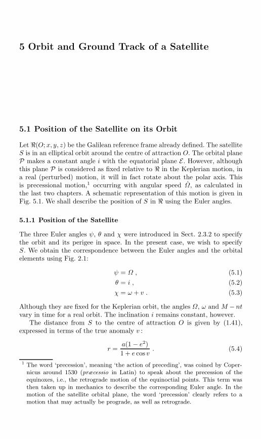
Let (O; x, y, z) be the Galilean reference frame already defined. The satelliteS is in an elliptical orbit around the centre of attraction O. The orbital planeP makes a constant angle i with the equatorial plane E . However, althoughthis plane P is considered as fixed relative to in the Keplerian motion, ina real (perturbed) motion, it will in fact rotate about the polar axis. Thisis precessional motion,1 occurring with angular speed Ω, as calculated inthe last two chapters. A schematic representation of this motion is given inFig. 5.1. We shall describe the position of S in using the Euler angles.
5.1.1 Position of the Satellite
The three Euler angles ψ, θ and χ were introduced in Sect. 2.3.2 to specifythe orbit and its perigee in space. In the present case, we wish to specifyS. We obtain the correspondence between the Euler angles and the orbitalelements using Fig. 2.1:
ψ = Ω , (5.1)θ = i , (5.2)χ = ω + v . (5.3)
Although they are fixed for the Keplerian orbit, the angles Ω, ω and M − ntvary in time for a real orbit. The inclination i remains constant, however.
The distance from S to the centre of attraction O is given by (1.41),expressed in terms of the true anomaly v :
r =a(1 − e2)1 + e cos v
. (5.4)
1 The word ‘precession’, meaning ‘the action of preceding’, was coined by Coper-nicus around 1530 (præcessio in Latin) to speak about the precession of theequinoxes, i.e., the retrograde motion of the equinoctial points. This term wasthen taken up in mechanics to describe the corresponding Euler angle. In themotion of the satellite orbital plane, the word ‘precession’ clearly refers to amotion that may actually be prograde, as well as retrograde.
176 5 Orbit and Ground Track of a Satellite
Figure 5.1. Precessional motion of the orbit in the frame . The orbital plane ro-tates about the polar axis, maintaining a fixed inclination relative to the equatorialplane (xOy). Its projection onto the equatorial plane can be used to measure Ω,the longitude of the ascending node, whose variation is given by Ω. If the satellitehas a prograde orbit (as here, where the ascending node has been indicated by asmall black circle, the descending node by a small white circle and the latest groundtrack by a dash-dotted curve), the precessional motion is retrograde, i.e., Ω < 0
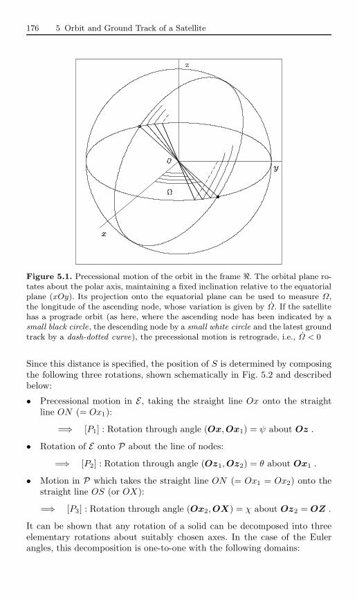
Since this distance is specified, the position of S is determined by composingthe following three rotations, shown schematically in Fig. 5.2 and describedbelow:
• Precessional motion in E , taking the straight line Ox onto the straightline ON (= Ox1):
=⇒ [P1] : Rotation through angle (Ox, Ox1) = ψ about Oz .
• Rotation of E onto P about the line of nodes:
=⇒ [P2] : Rotation through angle (Oz1, Oz2) = θ about Ox1 .
• Motion in P which takes the straight line ON (= Ox1 = Ox2) onto thestraight line OS (or OX):
=⇒ [P3] : Rotation through angle (Ox2, OX) = χ about Oz2 = OZ .
It can be shown that any rotation of a solid can be decomposed into threeelementary rotations about suitably chosen axes. In the case of the Eulerangles, this decomposition is one-to-one with the following domains:
5.1 Position of the Satellite on its Orbit 177
Figure 5.2. The three rotations taking a given point on a sphere to another ar-bitrary point, using the three Euler angles. Black circles indicate the three axes ofrotation: Oz = Oz1 for [P1], Ox1 = Ox2 for [P2], and Oz2 = OZ for [P3]
ψ ∈ [0, 2π) , θ ∈ [0, π) χ ∈ [0, 2π) .
The axes and angles of rotation are summarised here:
(Ox, Oy, Oz) P1−→ (Ox1, Oy1, Oz1 = Oz) ,
(Ox1, Oy1, Oz1)P2−→ (Ox2 = Ox1, Oy2, Oz2) ,
(Ox2, Oy2, Oz2)P3−→ (OX , OY , OZ = Oz2) .
We then have the three rotation matrices:
P1 =
⎛⎝ cosψ − sinψ 0sin ψ cosψ 0
0 0 1
⎞⎠ , (5.5)
P2 =
⎛⎝1 0 00 cos θ − sin θ0 sin θ cos θ
⎞⎠ , (5.6)
P3 =
⎛⎝ cosχ − sinχ 0sin χ cosχ 0
0 0 1
⎞⎠ . (5.7)
178 5 Orbit and Ground Track of a Satellite
The matrix product of these three matrices gives the matrix P calculatedbelow.
We consider without loss of generality that N is on the axis Ox at thetime origin. Its coordinates are thus (r, 0, 0). The coordinates of S(X, Y, Z)are obtained from those of N(x, y, z) via application of P :⎛⎝X
YZ
⎞⎠ = P
⎛⎝xyz
⎞⎠ = P
⎛⎝ r00
⎞⎠ .
We see that only the first column of the matrix P will be required for thiscalculation. We shall therefore calculate the matrix product P = P1P2P3 andwrite it in the form
P =
⎛⎝ cosψ cosχ − sin ψ sinχ cos θ P12 P13
sin ψ cosχ + cosψ sinχ cos θ P22 P23
sin χ sin θ P32 P33
⎞⎠ , (5.8)
which gives ⎛⎝XYZ
⎞⎠ = r
⎛⎝ cosψ cosχ − sin ψ sin χ cos θsinψ cosχ + cosψ sin χ cos θ
sinχ sin θ
⎞⎠ . (5.9)
Using the orbital parameters given by (5.1)–(5.4), we obtain⎛⎝XYZ
⎞⎠ =a(1 − e2)1 + e cos v
⎛⎝ cosΩ cos(ω + v) − sin Ω sin(ω + v) cos isinΩ cos(ω + v) + cosΩ sin(ω + v) cos i
sin(ω + v) sin i
⎞⎠ . (5.10)
Consider a spherical coordinate system in the Galilean frame . The planeof reference is the equatorial plane xOy of the Earth, Oz is the polar axisand the position of Ox is fixed in space.
The point S can be specified in by its spherical coordinates, the lon-gitude λ and the latitude φ, measured with the usual convention followingfrom the right-handed trigonometric system. The longitude of Ox (positionof N at the time origin) is denoted by λ0. Hence,⎛⎝X
YZ
⎞⎠ = r
⎛⎝ cosφ cos(λ − λ0)cosφ sin(λ − λ0)
sin φ
⎞⎠ . (5.11)
We thus obtain the position of S(λ, φ) as a function of time and the otherorbital parameters via X, Y, Z :
φ = arcsinZ
r, λ = λ0 + arccos
X
r cosφ, (5.12)
λ − λ0 from the sign of Y , λ − λ0 ∈ (−π, +π] . (5.13)
If |φ| = π/2, λ is not determined (and its determination would be pointless).
5.2 Ground Track of Satellite in Circular Orbit 179
5.1.2 Equation for the Ground Track
In many circumstances, one needs to know the position of the satellite relativeto the Earth. One must therefore represent S in the frame T, whose axesin the equatorial frame rotate with the Earth. The transformation from thisframe to the Galilean frame is obtained by a simple rotation about thepolar axis Oz with angular speed (−ΩT), since T rotates in with angularspeed ΩT. Bear in mind that these calculations are carried out in the Galileanframe , whilst the results may be expressed in the frame of our choice.
Recalling the above definition of λ0, the equations of motion of S are thesame in T as in , provided that we replace the value of ψ in (5.1) by
ψ = λ0 + (Ω − ΩT)(t − tAN) , (5.14)
where the time origin, the crossing time at the ascending node N , is writtent = tAN.
The satellite ground track is defined as the intersection of the straightline segment OS with the Earth’s surface. Its equation is thus obtained byreplacing r by R in the above equations. (For this application, we may treatthe Earth as a sphere of radius R.)
5.2 Ground Track of Satellite in Circular Orbit
Near-circular orbits, which may be considered as circular in a first approxi-mation, constitute a very important and frequently encountered case. Let usnow study some notions developed specifically for these orbits, such as theequatorial shift or the apparent inclination.
The velocity of the satellite will be calculated in Sect. 5.5.
5.2.1 Equation for Satellite Ground Track
When the orbit is circular, the motion is uniform with angular frequency n,the mean motion. Using the notation introduced above, the value of χ in(5.3) can be replaced by
χ = n(t − tAN) . (5.15)
We thus obtain the equation for the ground track, with (5.14), (5.2) and(5.15) substituted into (5.9) and (5.11), where r has been changed to R.
In this case, the ground track of the satellite is determined by two quan-tities relating to the ascending node taken as origin, namely, its longitudeλ0 and the crossing time tAN, which constitute the initial conditions of theuniform motion.
180 5 Orbit and Ground Track of a Satellite
Sun-Synchronous Satellites
For Sun-synchronous satellites, the angle ψ takes a specific value since Ω =ΩS. We have seen that the two angular frequencies characterising the Earth’s(annual and daily) motion are related by (4.24). Hence, according to (5.14),
ψ = ΩS − ΩT = − 2π
JM. (5.16)
Using the daily orbital frequency as given by (4.25), we obtain, for Sun-synchronous satellites, the very simple relation
ψ = −n
ν. (5.17)
We shall see the very important consequences of this relation in the followingchapters, in particular, when studying the crossing time of the satellite andthe question of recurrent orbits.
5.2.2 Maximum Latitude Attained
The ground track moves between two bounding latitudes, φ = +φm in thenorthern hemisphere and φ = −φm in the southern hemisphere. Consideringthe maximum positive value of Z, obtained for sinn(t− tAN) = 1, we obtain
sin φm = sin i , (5.18)
which implies that:
• for prograde satellites (0 i π/2), φm = i,• for retrograde satellites (π/2 i π), φm = π − i .
This value φm (φm 0) is called the maximum attained latitude.
Example 5.1. Calculate the maximal latitude attained by the Chinese satellite FY-1A, in Sun-synchronous orbit at an altitude of h = 901 km.
Given the altitude, we determine the inclination using (4.67). In the present exam-ple, we can use the simplified formula (4.74):
∆i = (901 − 800) × 4.17 × 10−3 ≈ 0.4 , i = i0 + ∆i = 98.6 + 0.4 = 99.0 ,
which yields the maximal attained latitude φm = 180− i = 81.0. Note that this is
the latitude reached by the ground track, not by oblique sightings by instruments
carried aboard. The ground track of the satellite thus remains within the bounding
latitudes 81N and 81S.
5.2 Ground Track of Satellite in Circular Orbit 181
5.2.3 Equatorial Shift
The difference in longitude between two consecutive ascending nodes λ1 andλ2 is called the equatorial shift and denoted by ∆λE, i.e.,
∆λE = λ2 − λ1 .
Rough Calculation
It is often sufficient to carry out a quick calculation of the equatorial shift,which is then denoted by ∆0λE. Indeed we may say to a first approximationthat, during one revolution of period T (and we may take the Keplerian periodhere), the orbit of the satellite will not have moved relative to , whilst theEarth makes one complete turn every day, i.e., it rotates through 15 perhour, or 1 every 4 min relative to this same frame. In this context, we donot bother with the precession of the orbit, or the Earth’s motion relative tothe Sun over the time taken for the satellite to complete one revolution. Thisamounts to using the relations ψ ≈ −ΩT and ΩT ≈ 2π/JM.
We have the simplified relation
∆0λE [degrees] = −T [min]4
, (5.19)
where the minus sign indicates a shift westwards. Observing that the valueof one degree of longitude is 111.3 km on the equator, we can also write
∆0λE [km] = −27.82T [min] . (5.20)
Using the daily orbital frequency ν (number of round trips per day), weobtain ∆0λE [degrees] = −360/ν and ∆0λE [km] ≈ −4 × 10⁴/ν.
Exact Calculation
During one revolution lasting T = Td, the orbital plane will have rotatedthrough an angle ψ with respect to T. The exact value of the equatorialshift as given by (5.14) with t − tAN = T is therefore
∆λE = ψT = −(ΩT − Ω)T . (5.21)
We note the following points, which follow from (5.21):
• The equatorial shift is always negative, since ΩT is greater than Ω. Theshift is westward for a satellite below the geosynchronous orbit.
• For satellites in Sun-synchronous orbit, we saw the specific value of ψ,according to (5.16). Over one nodal period T , we have
∆λE = ψT = − 2π
JMT . (5.22)
182 5 Orbit and Ground Track of a Satellite
Writing the angles in degrees and the time in minutes, we obtain (5.19).For a Sun-synchronous satellite, the approximate formula is identical tothe exact one. This is because the two approximations we made in therough calculation (neglecting precession and the annual motion of theEarth) exactly balance for this type of satellite.
• For satellites in geosynchronous orbit, T = 2π/ΩT and Ω is negligible.(In any case, it is not the leading term in the perturbation treatment forthis type of satellite.) In this case, we thus have
∆λE = −ΩTT = −2π = 0 mod (2π) . (5.23)
There is no equatorial shift for such a satellite. The projection of twoconsecutive ascending nodes does not move on the Earth. (If the satelliteis geostationary, we cannot even speak of an ascending node.)
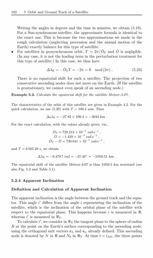
Example 5.2. Calculate the equatorial shift for the satellite Meteor-3-07.
The characteristics of the orbit of this satellite are given in Example 4.2. For thequick calculation, we use (5.20) with T = 109.4 min. Then
∆0λE = −27.82 × 109.4 = −3044 km .
For the exact calculation, with the values already given, viz.,
ΩT = 729.212 × 10⁻⁷ rad s−1 ,
Ω = −1.429 × 10⁻⁷ rad s−1 ,
ΩT − Ω = 730.641 × 10⁻⁷ rad s−1 ,
and T = 6565.28 s, we obtain
∆λE = −0.479 7 rad = −27.48 = −3 059.51 km .
The equatorial shift of the satellite Meteor-3-07 is thus 3 059.5 km westward (see
also Fig. 5.3 and Table 5.1).
5.2.4 Apparent Inclination
Definition and Calculation of Apparent Inclination
The apparent inclination is the angle between the ground track and the equa-tor. This angle i′ differs from the angle i representing the inclination of thesatellite, which is the inclination of the orbital plane of the satellite withrespect to the equatorial plane. This happens because i is measured in ,whereas i′ is measured in T.
To calculate i′, we consider in T the tangent plane to the sphere of radiusR at the point on the Earth’s surface corresponding to the ascending node,using the orthogonal unit vectors eλ and eφ already defined. This ascendingnode is denoted by N in and N0 in T. At time t = tAN, the three points
5.2 Ground Track of Satellite in Circular Orbit 183
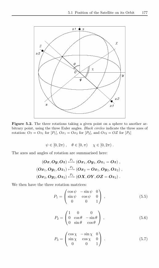
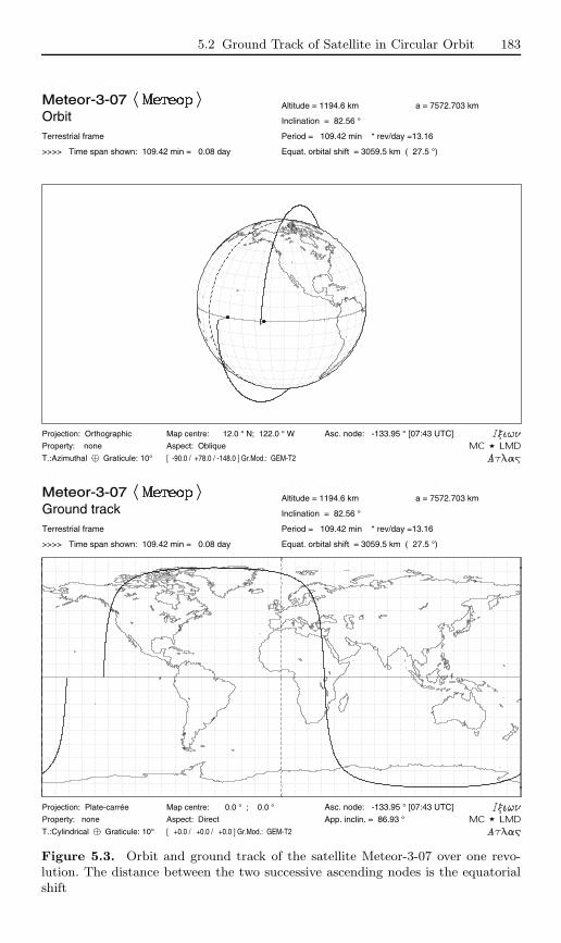
Meteor-3-07OrbitTerrestrial frame
>>>> Time span shown: 109.42 min = 0.08 day
Altitude = 1194.6 km a = 7572.703 km
Inclination = 82.56 °
Period = 109.42 min * rev/day =13.16
Equat. orbital shift = 3059.5 km ( 27.5 °)
Asc. node: -133.95 ° [07:43 UTC]Projection: Orthographic
Property: none
T.:Azimuthal Graticule: 10°
Map centre: 12.0 ° N; 122.0 ° W
Aspect: Oblique
[ -90.0 / +78.0 / -148.0 ] Gr.Mod.: GEM-T2
Meteor-3-07Ground trackTerrestrial frame
>>>> Time span shown: 109.42 min = 0.08 day
Altitude = 1194.6 km a = 7572.703 km
Inclination = 82.56 °
Period = 109.42 min * rev/day =13.16
Equat. orbital shift = 3059.5 km ( 27.5 °)
Asc. node: -133.95 ° [07:43 UTC]
App. inclin. = 86.93 °
Projection: Plate-carrée
Property: none
T.:Cylindrical Graticule: 10°
Map centre: 0.0 ° ; 0.0 °
Aspect: Direct
[ +0.0 / +0.0 / +0.0 ] Gr.Mod.: GEM-T2
Figure 5.3. Orbit and ground track of the satellite Meteor-3-07 over one revo-lution. The distance between the two successive ascending nodes is the equatorialshift

184 5 Orbit and Ground Track of a Satellite
Figure 5.4. Diagrams for the description of apparent inclination. (a) Inclination iand apparent inclination i′. The subsatellite point S0 and the point on the groundtrack corresponding to the ascending node have been represented in T. (b) Com-ponents of the satellite velocity in the frame T. The velocity vector v and itsprojection vxy onto the equatorial plane have been represented in the frame mov-ing with the Earth
S0 (the subsatellite point), N and N0 coincide. An infinitesimal time dt later,N and S0 have moved away from N0, as shown in Fig. 5.4a. In the frame T(N0, eλ, eφ), the components of the vectors N0N and NS0 are, settingdt = 1,
N 0N =(−(ΩT − Ω)
0
), NS0 =
(n cos in sin i
).
We thus deduce the components of N0S :
N0S =(
n cos i − (ΩT − Ω)n sin i
),
and the apparent inclination is given by
tan i′ =n sin i
n cos i − (ΩT − Ω). (5.24)
In terms of the daily recurrence frequency κ defined by (4.32), we may write
5.2 Ground Track of Satellite in Circular Orbit 185
tan i′ =sin i
cos i − (1/κ). (5.25)
Note that we always have i′ i.For a Sun-synchronous satellite, we may replace κ by ν, since according
to (4.33), these two daily frequencies are equal.
Example 5.3. Calculate the angle between the ground track of the TRMM satelliteand the equator when the satellite crosses the ascending node.
For TRMM (i = 34.98), we calculated the nodal precession rate in Example 4.1.We obtain
tan i′ =sin 34.98
cos 34.98 − 0.0649= 0.7604 ,
i′ = 37.25 , i′ − i = 2.27 .
Example 5.4. Calculate the apparent inclination for the ground track of a geosyn-chronous satellite.
For a geosynchronous satellite, we have ΩT/n = 1 and the term Ω is negligible.Equation (5.24) becomes
tan i′ =sin i
cos i − 1= − cos(i/2)
sin(i/2)= tan
„π
2+
i
2
«,
i′ = 90 +i
2, i′ − i = 90 − i
2.
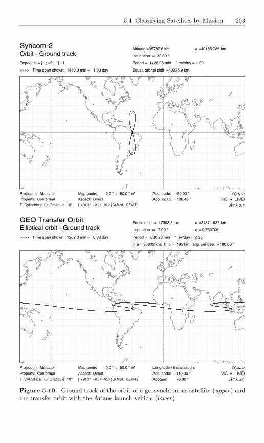
When i is very small, e.g., i = 1, we have i′ = 90.5: the ground track is not a point
but a small line segment almost perpendicular to the equator, between latitudes
1N and 1S, which transforms into a figure of 8 (lemniscate) when i increases,
growing larger with i. The first operational geosynchronous satellite, Syncom-2,
had inclination 32.8. Its ground track made an angle of 106.4 with the equator,
or an angle of 16.4 with the nodal meridian, as can be seen from the upper part
of Fig. 5.10.
Calculating the Inclination from the Apparent Inclination
We have obtained i′ as a function of i (and a). It is sometimes useful to do theopposite calculation, obtaining i as a function of i′ (and a). Using (4.1) andexpressing Ω/n by means of J2 and i, (5.24) can be replaced by the followingequation:
A cos i − B = C sin i , (5.26)
186 5 Orbit and Ground Track of a Satellite
where
A = 1 − 32J2
(R
a
)2
, B =ΩT
n, C =
1tan i′
. (5.27)
The aim now is to solve this for i. To begin with, we take n = n(a, i) = n0
in B so that this term does not depend on i. In a second step, we substituteinto B the value of n obtained using the previous value of i. The methodconverges very quickly.
Equation (5.26) transforms to a second order equation in tan(i/2). Thesolution, which is unique since the angle i lies in the interval [0, π], is givenby
tani
2=
−C +√
C2 + A2 − B2
A + B. (5.28)
We note that we have A ≈ 1, B ≈ 1/ν and hence B < A, except for satellitesin geosynchronous orbit or higher. This method allows one to find the incli-nation of a satellite of known altitude by measuring the apparent inclination,on a map of the ground track, for example. As we shall see below, it alsoallows one to calculate the inclination from the components of the velocityvector of the satellite.
Calculating the Inclination from the Satellite Velocity
The position and velocity of a satellite can be found either from the orbitbulletin or from remote-sensing data from the instruments aboard. The po-sition and velocity are given relative to the Earth. Let vX , vY , vZ be thevelocity components in T. At the ascending node, the angle between thevelocity vector, and hence the satellite trajectory, and the equatorial plane isthe apparent inclination.
Using Fig. 5.4b, we obtain the relation between i and the velocity atthe node (using the absolute value for the velocity components if the nodescannot be distinguished):
tan i′ =vZ√
v2X + v2
Y
. (5.29)
From the value for a and the value for i′ obtained in this way, we find i using(5.28).
Example 5.5. Calculate the inclination of the satellite Meteor-3-07 using the com-ponents of the velocity vector.
The values in Table 5.1 were obtained by interpolation of the raw remote-sensingdata collected during the first revolution in which the instrument ScaRaB was
5.2 Ground Track of Satellite in Circular Orbit 187
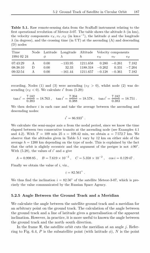
Table 5.1. Raw remote-sensing data from the ScaRaB instrument relating to thefirst operational revolution of Meteor-3-07. The table shows the altitude h (in km),the velocity components vX , vY , vZ (in km s−1), the latitude φ and the longitudeλ (in degrees), and the crossing time (in UT) at the ascending (A) and descending(D) nodes
Time Node Latitude Longitude Altitude Velocity components1994 02 24 φ λ h vX vY vZ
07:43:29 A 0.00 −133.95 1211.658 0.280 −0.261 7.18208:38:10 D 0.00 32.33 1188.318 −0.202 0.331 −7.20409:32:54 A 0.00 −161.44 1211.657 −0.128 −0.361 7.182
recording. Nodes (1) and (3) were ascending (vZ > 0), whilst node (2) was de-scending (vZ < 0). We calculate i′ from (5.29):
tan i′ =7.182
0.383= 18.763 , tan i′ =
7.204
0.388= 18.578 , tan i′ =
7.182
0.383= 18.751 .
We then deduce i in each case and take the average between the ascending anddescending nodes:
i′ = 86.933 .
We calculate the semi-major axis a from the nodal period, since we know the timeelapsed between two consecutive transits at the ascending node (see Examples 4.1and 4.2). With T = 109 min 25 s = 109.42 min, we obtain a = 7572.7 km. Weobserve that the altitudes given in Table 5.1 vary by 12 km on either side of theaverage h = 1200 km depending on the type of node. This is explained by the factthat the orbit is slightly eccentric and the argument of the perigee is not ±90.With (5.28), the values of i′ and a give
A = 0.998 85 , B = 7.619 × 10⁻² , C = 5.358 × 10⁻² , cos i = 0.129 47 .
Finally we obtain the value of i, viz.,
i = 82.561 .
We thus find the inclination i = 82.56 of the satellite Meteor-3-07, which is pre-
cisely the value communicated by the Russian Space Agency.
5.2.5 Angle Between the Ground Track and a Meridian
We calculate the angle between the satellite ground track and a meridian foran arbitrary point on the ground track. The calculation of the angle betweenthe ground track and a line of latitude gives a generalisation of the apparentinclination. However, in practice, it is more useful to known the angle betweenthe ground track and the north–south direction.
In the frame , the satellite orbit cuts the meridian at an angle j. Refer-ring to Fig. 6.4, P is the subsatellite point (with latitude φ), N is the point
188 5 Orbit and Ground Track of a Satellite
on the ground track corresponding to the ascending node (the dihedral angleat N gives the inclination i), and PQ is the meridian through P , where Qis on the equator. The dihedral angle at P is the angle j that we wish todetermine. Using the relation (ST V) with PQN for CAB, we obtain
sin j =cos i
cosφ. (5.30)
To calculate j′, we consider in T the plane tangent to the sphere of radiusR at the relevant point, with latitude φ, and orthogonal unit vectors eλ andeφ as already defined. As in the calculation of the apparent inclination, therelevant point is denoted by P in and P0 in T. At time t = tAN, the threepoints S0 (the subsatellite point), P and P0 coincide. After an infinitesimaltime dt (dt = 1), we obtain
P 0P =(−(ΩT − Ω) cosφ
0
), PS0 =
(n sin jn cos j
).
We deduce the components of P 0S :
P 0S =(
n sin j − (ΩT − Ω) cosφn cos j
).
This should be compared with (5.24).Using the daily frequency κ, we thus obtain
tan j′ =sin j − (1/κ) cosφ
cos j, (5.31)
and rewriting j,
tan j′ =cos i − (1/κ) cos2 φ√
cos2 φ − cos2 i. (5.32)
When the latitude of the point P equals the maximal attained latitude, onecan check that the ground track is in fact normal to the meridian.
5.3 Classifying Orbit Types
Satellite orbits can be classified according to various criteria: the inclination,the altitude, the eccentricity, or various properties.
Classification by Inclination
We have seen that the angle of inclination i of the orbit (angle of nutation θfor the Euler angles) is defined to lie between 0 and 180. If i is less than

5.3 Classifying Orbit Types 189
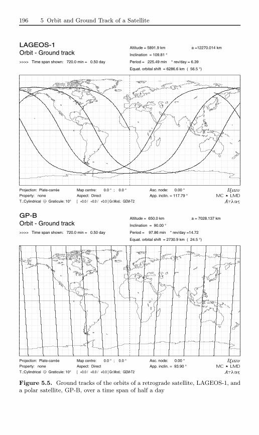
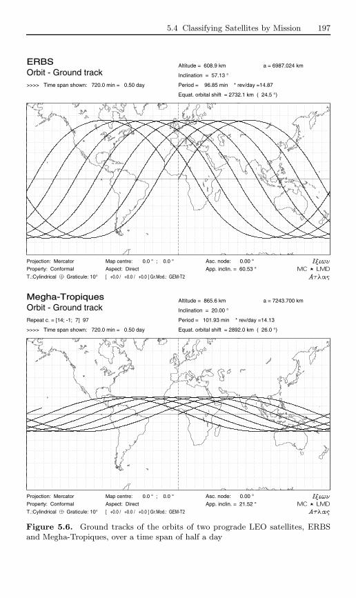
90, the orbit is prograde, whereas if i is greater than 90, it is retrograde.When i = 90, the orbit is polar. One may say strictly polar, because wheni lies between 80 and 100, one often describes it as a polar orbit, whereasnear-polar would be more appropriate. Figures 5.5 and 5.6 show the groundtracks of these orbits.
If i = 0 (or i = 180, although this has never happened), the orbit isequatorial, and for i less than 10, it is near-equatorial.
Classification by Altitude
Satellites in near-circular orbit are classified according to their mean altitude.We speak of a Low Earth Orbit (LEO) when the satellite flies at an altitudebelow 1 500 km, a Medium Earth Orbit (MEO) for GPS satellites at analtitude of around 20 000 km, and a Geostationary Earth Orbit (GEO) (alsosometimes called the Clarke orbit) for geostationary satellites at an altitudeof 36 000 km. We shall often use these abbreviations, which are concise andconsistent.2 Almost all satellites in orbits with low eccentricity fall into oneof these three categories. (For example, it is very rare, to find a satellite atan altitude of 8 000 km.)
For highly elliptical orbits,3 such as the Molniya or Tundra orbits, we usethe abbreviation HEO (Highly Eccentric Orbit). The name GTO (Geosta-tionary Transfer Orbit) is usually a temporary one, because the satellite hasbeen placed on this highly eccentric orbit for transfer towards a GEO orbit.Some satellites can be found in such orbits, some deliberately placed there,others because the apogee thrust used to make the orbit circular has beenunsuccessful. Finally, if a satellite has not been correctly placed in orbit, itis sometimes given the title FTO (Failed Transfer Orbit)!
The orbits L1LO and L2LO refer to halo orbits around the Lagrangepoints, which were discussed in Sect. 3.14.
Classification by Properties
When one needs to specify that a satellite is not geostationary, the termnon-geostationary satellite is used. Likewise a Sun-synchronous satellite iscontrasted with a non-Sun-synchronous satellite. We shall see other propertieslater, such as recurrent and frozen orbits.2 When we are referring to the satellite as LEO rather than the orbit, we un-
derstand of course ‘low Earth orbiting’ satellite. One does occasionally find theterm GEO meaning Geosynchronous Earth Orbit, as opposed to GSO for Geo-Stationary Orbit. In addition, and somewhat unnecessarily, one finds the termIGSO meaning Inclined GeoSynchronous Orbit for geosynchronous orbits thatare tilted and therefore not geostationary.
3 For Molniya-type orbits, the term THEO (Twelve Hour Eccentric Orbit) is some-times used. For very high orbits, like the orbit of Geotail, we use the term VHO(Very High Orbit).
190 5 Orbit and Ground Track of a Satellite
Orbit and Revolution
Since all scientific enterprise is based on a precise use of language, one mustmention a very common error which consists in saying ‘orbit’ instead of ‘rev-olution’ or ‘round trip’, an error which occurs in English, French and verylikely in other languages too. For example, we may read: the satellite Terra,during orbit 7778 . . . . This confusion is unjustified, and indeed, it is neverencountered in astronomy: one never says that the Moon makes one orbitaround the Earth every month.
5.4 Classifying Satellites by Mission
Our classification of satellites according to mission, which is of course ratherarbitrary, aims to illustrate the various types of orbit. We begin with satellitesdesigned for geophysics and Earth observation, then for navigation and com-munications, astronomy, technological development, and others that eludestraightforward classification. We shall touch briefly upon military satellitesand their specific missions, and satellites carrying humans.
The mission of a satellite often covers a range of different areas, e.g., anoceanographic satellite may also take part in a geodesy mission or a missionto develop altimetric techniques, and there has often been a large measureof ideology in satellite missions, especially at the beginning of the space age.However, we shall not be making a special entry for ideology!
With regard to military (or partly military) satellites the nomenclature isoften somewhat vague (even confused). From 1984, the United States calledsome of its satellites USA followed by a number specifying order of launch.Previously, these satellites had been called OPS followed by a four-figurenumber, without chronological ordering. (Between 1963 and 1984, close on500 OPS satellites were launched.) The USSR, then Russia, also created con-fusion with the Kosmos satellites: this name (from the Russian word kocmoc,originating itself from the Greek word , meaning ‘order’ or ‘wellordered’, hence ‘universe’) groups a whole multitude4 of satellites (not al-ways military), on every type of orbit and for every available type of mission.The People’s Republic of China did likewise with the appellation DFH (DongFang Hong, where ‘dong fang’ means ‘Orient’ and ‘hong’ means ‘red’), whichcovers the great majority of Chinese satellites. Without doing anything to4 The launch dates were as follows: Kosmos-1 on 16 March 1962, Kosmos-1001 on
4 April 1978, Kosmos-2001 on 14 February 1989. The launch rate then subsidedsomewhat. We give here the last Kosmos launched in the year: Kosmos-2054(1989), Kosmos-2120 (1990), Kosmos-2174 (1991), Kosmos-2229 (1992), Kosmos-2267 (1993), Kosmos-2305 (1994), Kosmos-2325 (1995), Kosmos-2336 (1996),Kosmos-2348 (1997), Kosmos-2364 (1998), Kosmos-2368 (1999), Kosmos-2376(2000), Kosmos-2386 (2001), Kosmos-2396 (2002), Kosmos-2404 (2003).
5.4 Classifying Satellites by Mission 191
simplify the situation, these satellites are also recorded by Western organisa-tions under the appellation PRC (People’s Republic of China), with anothernumbering system.
Satellites placed in orbit by the US Space Shuttle are noted: launched bySTS-(number). A satellite that is not specified in a series is denoted by -n(e.g., Molniya-n).
Launch dates are given up to 1 November 2004.
5.4.1 Geophysical Satellites
Geodesy
We have already mentioned these satellites in Chap. 3, where we gave acomplete list of the satellites used for the geopotential models EGM96S andGRIM5-S1.
The satellite Sputnik-1, the very first of all satellites, can be considered asa geodesy satellite. At the beginning of space geodesy, many satellites wereplaced above the LEO altitude so as to reduce atmospheric drag. Examplesare PAGEOS, launched in 1966, between 3 000 and 5 200 km, with i = 84.4,the two LAGEOS (Laser Geodynamics Satellite), with h = 5 900 km andinclinations i = 109.8 for LAGEOS-1, launched in 1976 and i = 52.6 forLAGEOS-2, launched in 1992 by STS-52. The ground track of the orbit ofLAGEOS-1 is shown in Fig. 5.5 (upper).
The satellites SECOR-7, -8, -9 orbit at 3 700 km altitude and the Sovietsatellites Etalon-1 and -2 (Kosmos-1989 and -2024), launched in 1989 withGLONASS, are in a circular MEO orbit, h = 19 130 km, i = 64.8. Othersare at altitudes between 1500 and 1000 km: the fifteen Soviet satellites Geo-1K, such as Kosmos-2226, the French satellite Starlette and the US pioneerAnna-1B, launched in 1962, h = 1 120 km, i = 50.1.
The Japanese satellite LRE (Laser Ranging Experiment), launched intoeccentric orbit in 2001, hp = 271 km, ha = 36 214 km, i = 28, is equippedwith 126 laser reflectors.
There are some Sun-synchronous satellites between 800 and 1 000 km,such as TOPO-1 and those launched after 1993, Stella and Westpac-1 (Sun-synchronous because they are microsatellites that were themselves launchedby Sun-synchronous satellites). Since then, geodesy satellites have beenplaced in lower orbits. An example is GFZ-1 (Geo Forschungs Zentrum),launched in 1995, h = 380 km, i = 51.6.
Our knowledge of the geopotential has become so precise that a wholenew generation of geodesy satellites5 was put in operation in 2000. Theycarry ultra-sensitive accelerometers. Their altitudes must be as low as pos-sible for better detection of gravitational anomalies, whilst a continuousthrust compensates for the higher level of atmospheric drag. The German5 Launch dates: CHAMP on 15 June 2000, GRACE-A and -B on 17 March 2002.
192 5 Orbit and Ground Track of a Satellite
satellite CHAMP (Challenging Minisatellite Payload for geophysical researchand applications) is on a near-polar orbit i = 87.3 with an initial altitudeh = 454 km (h = 300 km after 5 years, mission lifetime). The US–Germansystem GRACE (Gravity Recovery And Climate Experiment) comprises twosatellites, GRACE-A and GRACE-B, 220 km apart on the same orbit ath = 485 km, i = 89.5. The altitude should drop down to 250 km over thefive-year lifetime of the two satellites. The experiment involves measuring therelative speed of the two satellites to an accuracy of 1 µm s−1. This allowsone to detect very weak fluctuations in the Earth’s gravitational field andhence to follow the movement of water in the Earth’s hydrological cycle.
The European project GOCE (Gravity field and steady state Ocean Cir-culation Experiment) uses a Sun-synchronous satellite at very low altitude,6
i.e., h ≈ 250 km.
Earth Environment: Ionosphere and Magnetosphere
To study the Earth’s magnetic field, two satellites are in Sun-synchronousLEO, but elliptical orbit, namely MAGSAT (Magnetic field Satellite, AEM-3), launched in 1979, hp = 352 km, ha = 561 km, i = 96.8, and the DanishØrsted, launched in 1999, hp = 450 km, ha = 850 km, i = 96.5. To studythe radiation belts, the Chinese satellite SJ-5 (Shi Jian-5, DFH-47, where ‘shijian’ means ‘achievement’), launched in 1999, at the same time as FY-1C, isin a circular Sun-synchronous orbit with h = 855 km. SJ-6A and SJ-6B,launched in 2004, are in a lower orbit, h = 602 km.
In near-polar LEO orbit, between 800 and 1000 km, are the even-numbered OGO satellites (Orbiting Geophysical Observatory), OGO-2, -4,-6, called POGO (Polar OGO), launched between 1965 and 1969, the Swedishsatellites Astrid-1 and -2, launched in 1995 and 1998, and the strictly polarsatellite Polar BEAR (Beacon Experiments and Auroral Research).
To study the magnetosphere, that is, the zone of interaction betweenparticles excited by the solar wind and the Earth’s magnetic field, satelliteorbits have to be very high and highly elliptical. The first US satellite7 to beplaced in orbit, Explorer-1, launched on 11 February 1958, with hp = 347 km,ha = 1 859 km, i = 33.2, already had some of these features. Its masswas only 5 kg, but it discovered two radiation belts around the Earth, since6 At this altitude, and for this 800 kg satellite, the acceleration due to atmospheric
drag is 1.5 × 10⁻⁵ m s−2, whilst the acceleration due to radiation pressure is6.1× 10−8 m s−2. As a comparison, these values are respectively 6.0× 10⁻⁸ and3.7×10−8 for µSCOPE, a 120kg satellite planned for circular orbit at an altitudeof 700 km.
7 Following the Soviet launch of the two Sputniks, the United States wished toreact very quickly. The first US satellite was to be a Vanguard, prepared by theUS Navy, but in the end it was an Explorer of the US Army that was first placedin orbit. This competition between the two branches of the armed forces cameto an end when NASA was created on 1 October 1958.
5.4 Classifying Satellites by Mission 193
referred to as the Van Allen belts. This radiation was studied by the SovietElektron programme for which four satellites were launched in two pairs in1964: Elektron-1 and -2, Elektron-3 and -4. They all followed eccentric orbits,with inclination i ≈ 61, and with ha ≈ 6 500 km for the odd numbers,ha ≈ 65 000 km for the even numbers.
Magnetospheric studies continued with a great many satellites launchedbetween 1964 and 1968, such as the odd-numbered OGO satellites, OGO-1,-3, -5, known as EOGO (Eccentric OGO), Explorer-34 (IMP-F or IMP-5,Interplanetary Monitoring Platform), launched in 1967 with hp = 242 km,ha = 214 400 km, i = 67.1, or Explorer-50 (IMP-J or IMP-8), launched intoa very high orbit in 1973 with variable inclination between 32 and 55 (andafter thirty years, this satellite is still operational).
For the ISEE experiment (International Sun–Earth Explorer), the twosatellites ISEE-1 and -2 were launched in 1977, on highly eccentric orbits:hp ≈ 400 km, ha ≈ 138 000 km, i = 12.7 and 13.5. Then in 1978, ISEE-3was the first satellite placed in a halo orbit8 around the Lagrange point L1,i.e., the halo orbit known as L1LO (see Sect. 3.14).
The satellite Wind, launched in 1994, was also placed in an L1LO orbitaround the point L1, where it remained from May 1997 until April 1998.From this location, it was able to observe the solar wind before it becameperturbed by the Earth’s magnetosphere. It was subsequently placed on ahighly complex orbit known as a petal orbit from November 1998 to April1999.9 The satellite ACE (Advanced Composition Explorer), launched in1997, is also in an L1LO orbit.
We should also mention the highly eccentric orbits of the followingsatellites: Geotail, a Japanese satellite launched in 1992, hp = 41 360 km,ha = 508 500 km, i = 22.4; Polar, launched in 1996, on an orbit with vari-able parameters,10 a ≈ 60 000 km, e ≈ 0.7, i ≈ 80 (several revolutions are
8 When it had accomplished its mission, the satellite was withdrawn from the pointL1 in June 1982. Using a lunar flyby as a gravity-assist maneuver, it was removedfrom the Earth’s gravitational attraction and sent into heliocentric orbit for theICE mission (International Cometary Explorer), in an encounter with a comet(perihelion 0.93 a.u., aphelion 1.03 a.u., inclination 0.1, period 355 day).
9 The satellite left the point L1 in the Earthward direction, roughly in the planeof the lunar orbit, before moving into the petal orbit. In this configuration, thesatellite moves alternately behind the Earth and the Moon. In this plane andin a frame moving with the Earth, the trajectory sketches out a daisy with theEarth at the centre. The tips of the petals represent the different positions of theMoon in its rotation about the Earth. It has period 17.5 day, radius of ellipserp ≈ 6 to 10R, ra ≈ 80R (where the Earth–Moon distance is 60R).
10 The orbit shown in the figure is that of 13 February 2002. This satellite, the PolarPlasma Laboratory, is part of the GGS mission (Global Geospace Science) withWind and Geotail, and this is itself just one component of the ISTP programme(International Solar Terrestrial Physics), which includes the European missionsSOHO and Cluster and the Russian mission Interball.
194 5 Orbit and Ground Track of a Satellite
shown in the lower part of Fig. 5.22); FAST (Fast Auroral Snapshot Ex-plorer, SMEX-2), launched in 1996, hp = 353 km, ha = 4 163 km, i = 83.0
(see lower part of Fig. 5.21 for orbit in November 2004); Equator-S, launchedin 1997, hp = 496 km, ha = 67 230 km, i = 7.0 (orbit obtained by transfervia a GTO orbit); IMAGE (Imager for Magnetopause-to-Aurora Global Ex-ploration, MIDEX-1), launched in 2000, on a polar orbit with hp ≈ 1000 kmand ha of the order of 7 Earth radii.
The Russian Interball experiment is based on Interball Tail (or Interbol-1,Prognoz-11), launched in 1995 on a highly elliptical orbit with period T =91 hr, and Interball Aurora (or Interbol-2, Prognoz-12), launched in 1996 ona Molniya orbit. In each case, the Czech satellites Magion (Magnetosphere–Ionosphere), Magion-4, then Magion-5, were launched jointly with an In-terball satellite. The orbit of the forthcoming Interbol-3 is planned forha = 400 000 km. We also mention the Chinese satellite KF1-SJ-4 (Shi Jian-4,DFH-38), launched in 1994, on a GTO orbit, with i = 28.6.
To study the magnetosphere and phenomena related to the aurora bo-realis, Japan sent four satellites EXOS (Exospheric Observations) between1978 and 1989, in alternately low and high eccentric orbits, with i = 69 forEXOS-A (Kyokko), i = 31 for EXOS-B (Jikiken), and i = 75 for EXOS-C(Ohzora) and EXOS-D (Akebono).
The European experiment Cluster-2 comprises four satellites in forma-tion.11 They have a very high orbit, with hp = 17 200 km, ha = 120 600 km,i = 65, T = 57 hr.
The Double Star programme comprises two Chinese satellites carryingEuropean satellites similar to those designed for Cluster, in eccentric orbits,12
with perigee at 600 km altitude. The first, DSP-1, ha = 79 000 km, is in anequatorial orbit, and the second, DSP-2, ha = 39 000 km, is in polar orbit.
To study the ionosphere,13 there are the US satellites UARS (Upper At-mosphere Research Satellite), h = 570 km, i = 56.9, and TIMED (Thermo-Iono-Mesosphere Energetics and Dynamics), h = 625 km, i = 74.0. In addi-tion, there is the Taiwanese satellite Rocsat-1 (Republic of China Satellite),with a slightly inclined orbit, h = 630 km, i = 35 (for oceanographic pur-poses) and many Interkosmos, such as Interkosmos-12, several Kosmos, suchas Kosmos-196, and the Chinese satellites Atmosphere-1 and -2 (DFH-31
11 These satellites, Rumba, Salsa, Samba and Tango, fly a few hundred kilometresapart. They were launched in two stages, on 16 June and 19 August 2000, toavoid repetition of the disaster when Cluster was launched together on 4 June1996.
12 DSP-1 (also called Tan Ce-1 – Explorer-1 in Chinese – or TC-1), a = 46 148.1 km,e = 0.8494, i = 28.5, launched on 29 December 2003. DSP-2 (Tan Ce-2 or TC-2), a = 26 228.1 km, e = 0.7301, i = 90, launched on 25 July 2004.
13 Launch dates: UARS on 12 September 1991 (STS-48), TIMED 7 on Decem-ber 2001 (with Jason-1 but in a different orbit), Rocsat-1 on 27 January 1999,Interkosmos-12 on 30 October 1974, Atmosphere-1 and -2 (DFH-31 and -32) on3 September 1990, SAMPEX on 3 July 1992, TERRIERS on 18 May 1999.
5.4 Classifying Satellites by Mission 195
and -32), which are Sun-synchronous with h = 800 km and h = 610 km. Thesatellite SAMPEX (Solar Anomalous and Magnetospheric Particle Explorer,SMEX-1) is near-polar, with hp = 506 km, ha = 670 km, i = 81.7. TheUS satellite TERRIERS, is Sun-synchronous with h = 550 km, but did notfunction as planned.
5.4.2 Earth-Observation Satellites
Atmosphere and Meteorology
The possibility of observation from space aroused the interest of meteorol-ogists from an early stage. It was their dream to know the global state ofthe atmosphere at a glance. In order to do so, the orbits used have alwaysbeen Sun-synchronous LEO orbits (see Fig. 5.7) or GEO orbits (see Fig. 5.8),apart from the first satellites and the Meteor satellites.
LEO Meteorological Satellites. For NASA’s Nimbus programme14 allseven satellites were Sun-synchronous: from Nimbus-1 to Nimbus-6, on arather high LEO orbit, h = 1 100 km, i = 99.9, whilst Nimbus-7 followed aslightly lower orbit, h = 950 km, i = 99.1.
The programme which is known today as the NOAA programme (Na-tional Oceanic and Atmospheric Administration), the US meteorological or-ganisation, can be divided into five series: TIROS (Television and InfraRedObservation Satellite), TOS (TIROS Operational System), ITOS (ImprovedTOS), TIROS-N and ATN (Advanced TIROS-N). The first comprises twelvesatellites and began on 1 April 1960 with the launch of the first meteorologicalsatellite,15 TIROS-1. Up to TIROS-8, launched in 1963, the orbits were sim-ilar, h ≈ 680 km, i between 48 and 58. Subsequently, all further satelliteswere Sun-synchronous: TIROS-9 and -10, launched in 1964, and ESSA-1 and-2 (Environmental Science Service Administration), launched in 1966. TheTOS series comprised seven satellites, from ESSA-3 to ESSA-9, launched be-tween 1966 and 1969, on the orbit h = 1 450 km, i = 102. The ITOS seriesused exactly the same orbit for six satellites, ITOS-1, NOAA-1, -2, -3, -4,-5, launched between 1970 and 1976. The last two series16 adopted a lowerorbit: h = 800 km, i = 98.8 for TIROS-N, with the satellites TIROS-N and14 Launch dates: Nimbus-1 on 28 August 1964, Nimbus-2 on 15 May 1966, Nimbus-
3 on 14 April 1969, Nimbus-4 on 8 April 1970, Nimbus-5 on 11 December 1972,Nimbus-6 on 12 June 1975, Nimbus-7 on 24 October 1978.
15 The three US satellites launched in 1959 had provided useful meteorologicaldata. These were Vanguard-2, Explorer-6 (first photograph of the Earth) andExplorer-7 (first data concerning the Earth radiation budget). However, the firstdevoted entirely to meteorology was TIROS-1.
16 Launch dates: TIROS-N on 13 October 1978, NOAA-6 on 27 June 1979, NOAA-7 on 23 June 1981, NOAA-8 on 28 March 1983, NOAA-9 on 12 December 1984,NOAA-10 on 17 December 1986, NOAA-11 on 24 September 1988, NOAA-12 on
196 5 Orbit and Ground Track of a Satellite
LAGEOS-1Orbit - Ground track>>>> Time span shown: 720.0 min = 0.50 day
Altitude = 5891.9 km a =12270.014 km
Inclination = 109.81 °
Period = 225.49 min * rev/day = 6.39
Equat. orbital shift = 6286.6 km ( 56.5 °)
Asc. node: 0.00 °
App. inclin. = 117.79 °
Projection: Plate-carrée
Property: none
T.:Cylindrical Graticule: 10°
Map centre: 0.0 ° ; 0.0 °
Aspect: Direct
[ +0.0 / +0.0 / +0.0 ] Gr.Mod.: GEM-T2
GP-BOrbit - Ground track>>>> Time span shown: 720.0 min = 0.50 day
Altitude = 650.0 km a = 7028.137 km
Inclination = 90.00 °
Period = 97.86 min * rev/day =14.72
Equat. orbital shift = 2730.9 km ( 24.5 °)
Asc. node: 0.00 °
App. inclin. = 93.90 °
Projection: Plate-carrée
Property: none
T.:Cylindrical Graticule: 10°
Map centre: 0.0 ° ; 0.0 °
Aspect: Direct
[ +0.0 / +0.0 / +0.0 ] Gr.Mod.: GEM-T2
Figure 5.5. Ground tracks of the orbits of a retrograde satellite, LAGEOS-1, anda polar satellite, GP-B, over a time span of half a day
5.4 Classifying Satellites by Mission 197
ERBSOrbit - Ground track>>>> Time span shown: 720.0 min = 0.50 day
Altitude = 608.9 km a = 6987.024 km
Inclination = 57.13 °
Period = 96.85 min * rev/day =14.87
Equat. orbital shift = 2732.1 km ( 24.5 °)
Asc. node: 0.00 °
App. inclin. = 60.53 °
Projection: Mercator
Property: Conformal
T.:Cylindrical Graticule: 10°
Map centre: 0.0 ° ; 0.0 °
Aspect: Direct
[ +0.0 / +0.0 / +0.0 ] Gr.Mod.: GEM-T2
Megha-TropiquesOrbit - Ground trackRepeat c. = [14; -1; 7] 97
>>>> Time span shown: 720.0 min = 0.50 day
Altitude = 865.6 km a = 7243.700 km
Inclination = 20.00 °
Period = 101.93 min * rev/day =14.13
Equat. orbital shift = 2892.0 km ( 26.0 °)
Asc. node: 0.00 °
App. inclin. = 21.52 °
Projection: Mercator
Property: Conformal
T.:Cylindrical Graticule: 10°
Map centre: 0.0 ° ; 0.0 °
Aspect: Direct
[ +0.0 / +0.0 / +0.0 ] Gr.Mod.: GEM-T2
Figure 5.6. Ground tracks of the orbits of two prograde LEO satellites, ERBSand Megha-Tropiques, over a time span of half a day

198 5 Orbit and Ground Track of a Satellite
NOAA-6 and -7; h = 850 km, i = 98.9 for ATN, with the satellites NOAA-8 to -16, h = 812 km, i = 98.8 for NOAA-17. The programme known asPOES (Polar-orbiting Operational Environmental Satellites), comprising thelast two series, should be replaced around 2010 by the programme NPOESS(National POES System), a joint project of NOAA and NASA. The pro-grammes will be linked by the satellite NPP (NPOESS Preparatory Project),h = 824 km.
The military satellites DMSP (Defense Meteorological Satellite Program)supply some data to the civilian sector. They are all Sun-synchronous, follow-ing slightly elliptical orbits, with h between 750 and 850 km, and i between98.6 and 99.2. Thirteen satellites were launched between 1965 and 1969 tomake up the first block (known as Block 4), from DMSP-4A F-1 (OPS/6026)to DMSP-4A F-13 (also called DMSP-4B F-3, or OPS/1127). The secondblock (known as Block 5) began in 1970 with DMSP-5A F-1 (OPS/0054)and is still running,17 with the extension Block 5D3.
Soviet then Russian meteorological satellites18 were not Sun-synchronousuntil 2001. They are divided into three Meteor series with near-polar LEOorbits. The first two series involved 48 satellites: Meteor-1, from Meteor-1-01in 1969 to Meteor-1-27 in 1977, with h = 870 km, i = 81.2; Meteor-2, fromMeteor-2-01 in 1975 to Meteor-2-21 in 1993, with h = 940 km, i = 82.5. Thethird series involved 6 satellites in slightly higher orbits, with h = 1 200 km,i = 82.6. The new generation, known as Meteor-3M, is Sun-synchronous.The first of the series is Meteor-3M-1, h = 1 005 km, i = 99.7.
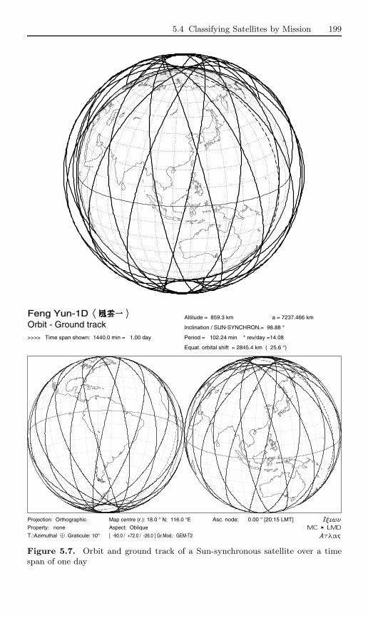
The Chinese satellites19 in the FY-1 series (or Feng Yun-1, where ‘fengyun’ means ‘wind and cloud’) are Sun-synchronous, with h = 858 km, i =98.9.
The European Space Agency has a programme of (Sun-synchronous) polarplatforms. The initial programme POEM (Polar Orbiting Earth Mission)
14 May 1991, NOAA-13 on 9 August 1993, but only operated for a few days,NOAA-14 on 30 December 1994, NOAA-15 on 13 May 1998, NOAA-16 on 21September 2000, NOAA-17 on 24 June 2002.
17 Launch dates: DMSP-5D2 F-8 (also called USA-26) on 20 June 1987, DMSP-5D2 F-9 (USA-29) on 3 February 1988, DMSP-5D2 F-10 (USA-68) on 1 Decem-ber 1990, DMSP-5D2 F-11 (USA-73) on 28 November 1991, DMSP-5D2 F-12(USA-106) on 29 August 1994, DMSP-5D2 F-13 (USA-109) on 24 March 1995,DMSP-5D2 F-14 (USA-131) on 4 April 1997, DMSP-5D3 F-15 (USA-147) on 12December 1999, and DMSP-5D3 F-16 (USA-172) on 18 October 2003.
18 Launch dates: Meteor-3-01 on 24 October 1985, Meteor-3-03 on 26 July 1988,Meteor-3-04 on 25 October 1989, Meteor-3-05 on 24 April 1991, Meteor-3-06 on15 August 1991, Meteor-3-07 on 25 January 1994, Meteor-3M-1 on 10 December2001.
19 Launch dates: FY-1A (DFH-24) on 6 September 1988, FY-1B (DFH-30) on 3September 1990, FY-1C (DFH-46) on 10 May 1999, FY-1D (DFH-53) on 15 May2002. The next series of Sun-synchronous LEO satellites is FY-3, from FY-3Ato FY-3D.
5.4 Classifying Satellites by Mission 199
Feng Yun-1DOrbit - Ground track>>>> Time span shown: 1440.0 min = 1.00 day
Altitude = 859.3 km a = 7237.466 km
Inclination / SUN-SYNCHRON.= 98.88 °
Period = 102.24 min * rev/day =14.08
Equat. orbital shift = 2845.4 km ( 25.6 °)
Asc. node: 0.00 ° [20:15 LMT]Projection: Orthographic
Property: none
T.:Azimuthal Graticule: 10°
Map centre (r.): 18.0 ° N; 116.0 °E
Aspect: Oblique
[ -90.0 / +72.0 / -26.0 ] Gr.Mod.: GEM-T2
Figure 5.7. Orbit and ground track of a Sun-synchronous satellite over a timespan of one day
200 5 Orbit and Ground Track of a Satellite
0°
30°E
60°E
90°E
120°E
150°E
180°
150°W
120°W
90°W
60°W
30°W
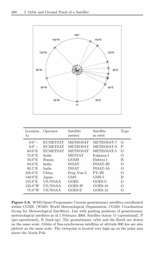
Location Operator Satellite Satellite TypeλS (series) in orbit
0.0− EUMETSAT METEOSAT METEOSAT-7 O0.0− EUMETSAT METEOSAT METEOSAT-8 P
63.0E EUMETSAT METEOSAT METEOSAT-5 O74.0E India METSAT Kalpana-1 O76.0E Russia GOMS Elektro-1 B83.0E India INSAT INSAT-2E O93.5E India INSAT INSAT-3A O
105.0E China Feng Yun-2 FY-2B O140.0E Japan GMS GMS-5 B155.0E US/NOAA GOES GOES-9 O135.0W US/NOAA GOES-W GOES-10 O75.0W US/NOAA GOES-E GOES-12 O
Figure 5.8. WMO Space Programme: Current geostationary satellites coordinatedwithin CGMS. (WMO: World Meteorological Organization; CGMS: CoordinationGroup for Meteorological Satellites). List with parking positions of geostationarymeteorological satellites as of 1 February 2004. Satellite status: O (operational), P(pre-operational), B (back-up). The geostationary orbit and the Earth are drawnon the same scale. Orbits of Sun-synchronous satellites at altitude 800 km are alsoplotted on the same scale. The viewpoint is located very high up on the polar axisabove the North Pole
5.4 Classifying Satellites by Mission 201
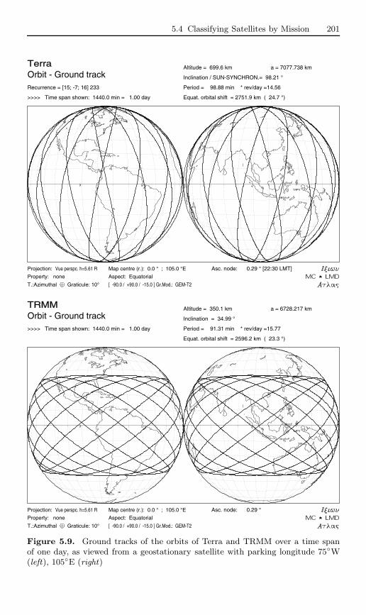
TerraOrbit - Ground trackRecurrence = [15; -7; 16] 233
>>>> Time span shown: 1440.0 min = 1.00 day
Altitude = 699.6 km a = 7077.738 km
Inclination / SUN-SYNCHRON.= 98.21 °
Period = 98.88 min * rev/day =14.56
Equat. orbital shift = 2751.9 km ( 24.7 °)
Asc. node: 0.29 ° [22:30 LMT]Projection: Vue perspc. h=5.61 R
Property: none
T.:Azimuthal Graticule: 10°
Map centre (r.): 0.0 ° ; 105.0 °E
Aspect: Equatorial
[ -90.0 / +90.0 / -15.0 ] Gr.Mod.: GEM-T2
TRMMOrbit - Ground track>>>> Time span shown: 1440.0 min = 1.00 day
Altitude = 350.1 km a = 6728.217 km
Inclination = 34.99 °
Period = 91.31 min * rev/day =15.77
Equat. orbital shift = 2596.2 km ( 23.3 °)
Asc. node: 0.29 °Projection: Vue perspc. h=5.61 R
Property: none
T.:Azimuthal Graticule: 10°
Map centre (r.): 0.0 ° ; 105.0 °E
Aspect: Equatorial
[ -90.0 / +90.0 / -15.0 ] Gr.Mod.: GEM-T2
Figure 5.9. Ground tracks of the orbits of Terra and TRMM over a time spanof one day, as viewed from a geostationary satellite with parking longitude 75W(left), 105E (right)
202 5 Orbit and Ground Track of a Satellite
was divided into two parts, one for the environment with Envisat, the otherfor operational meteorology (EUMETSAT) with MetOp-1, -2 and -3. TheMetOp satellites (Meteorological Operational satellites) are planned for amean altitude of h = 830 km.
The project known as Rocsat-3/COSMIC (Constellation Observing Sys-tem for Meteorology, Ionosphere and Climate), a collaboration between Tai-wan and the United States, comprises a constellation of microsatellites,h = 700 km, i = 72, with 3 planes containing 2 satellites each.
GEO Meteorological Satellites. The geostationary programme has beenvery widely developed for the purposes of operational meteorology. In orderto avoid large distortions due to the viewing angle, the various meteorologi-cal institutions have sought to distribute their satellites as harmoniously aspossible around the geostationary orbit, under the coordination of the WorldMeteorological Organization (WMO).
In the United States, these satellites are placed alternately on the lon-gitudes of the east and west coasts. This approach was already in use forthe SMS satellites (SMS-1 with λS = 75W, SMS-2 with λS = 115W) andwas continued with the GOES series20 (Geostationary Operational Environ-mental Satellite) and GOES-Next, the satellites being designated GOES-East or GOES-West depending on the case. The satellite GIFTS (Geosyn-chronous Imaging Fourier Transform Spectrometer, or EO-3 NMP/NASA)will be placed over the Indian Ocean.
For Europe, the geostationary programme is run by EUMETSAT with theMETEOSAT satellites. The various operational METEOSAT spacecraft21
have all been placed at longitude λS = 0. Some of them can be reserved,or loaned (like METEOSAT-3 to replace GOES-E from February 1993 toMay 1995), or sent on missions (such as METEOSAT-5 for the INDOEXexperiment, see Example 4.6).
Although Russia generally prefers Molniya orbits to equatorial orbits,it nevertheless launched the GOMS programme (Geostationary Operational
20 Launch dates: SMS-1 on 17 May 1974, SMS-2 on 6 February 1975, GOES-1(SMS-3) on 16 October 1975, GOES-2 on 16 June 1977, GOES-3 on 16 June1978, GOES-4 on 9 September 1980, GOES-5 on 22 May 1981, GOES-6 on 28April 1983, GOES-7 on 26 February 1987, GOES-8 on 13 April 1994, GOES-9on 23 May 1995, GOES-10 on 25 April 1997, GOES-11 on 3 May 2000, GOES-12on 23 July 2001.
21 Launch dates: METEOSAT-1 on 23 November 1977, METEOSAT-2 on 19June 1981, METEOSAT-3 on 15 June 1988, METEOSAT-4 on 6 March1989, METEOSAT-5 on 2 March 1991, METEOSAT-6 on 20 November 1993,METEOSAT-7 on 2 September 1997, MGS-1 (METEOSAT-8) on 28 August2002. The satellite MSG-1, the first in the MSG series (METEOSAT Second Gen-eration), was renamed METEOSAT-8 when it became operational. The satellitesMSG-2, -3 and -4 are programmed, and MTG-1 (METEOSAT Third Generation)is planned for 2015.
5.4 Classifying Satellites by Mission 203
Syncom-2Orbit - Ground trackRepeat c. = [ 1; +0; 1] 1
>>>> Time span shown: 1440.0 min = 1.00 day
Altitude =35787.6 km a =42165.785 km
Inclination = 32.80 °
Period = 1436.05 min * rev/day = 1.00
Equat. orbital shift =40075.9 km
Asc. node: -50.00 °
App. inclin. = 106.40 °
Projection: Mercator
Property: Conformal
T.:Cylindrical Graticule: 10°
Map centre: 0.0 ° ; 50.0 ° W
Aspect: Direct
[ +90.0 / +0.0 / -40.0 ] Gr.Mod.: GEM-T2
GEO Transfer OrbitElliptical orbit - Ground track>>>> Time span shown: 1262.0 min = 0.88 day
Equiv. altit. = 17993.5 km
e = 0.730706
a =24371.637 km
Inclination = 7.00 °
Period = 630.23 min * rev/day = 2.28
h_a = 35802 km; h_p = 185 km; arg. perigee: +180.00 °
Longitude / Initialisation:
Asc. node: -110.00 °
Apogee: 70.00 °
Projection: Mercator
Property: Conformal
T.:Cylindrical Graticule: 10°
Map centre: 0.0 ° ; 50.0 ° W
Aspect: Direct
[ +90.0 / +0.0 / -40.0 ] Gr.Mod.: GEM-T2
Figure 5.10. Ground track of the orbit of a geosynchronous satellite (upper) andthe transfer orbit with the Ariane launch vehicle (lower)
204 5 Orbit and Ground Track of a Satellite
Meteorological Satellite) of geostationary satellites.22 For India, the INSATseries (Indian Satellite) contains satellites for the purposes of meteorology23
and communications. China has launched satellites24 in the FY-2 series (FengYun-2, not to be confused with the LEO satellite series FY-1 and FY-3 al-ready mentioned) since 1997. Since 1977, Japan has been launching its geosta-tionary GMS satellites25 (Geostationary Meteorological Satellite), also knownas Himawari (‘himawari’ means ‘sunflower’).
Figure 5.8 shows the (official) positions of the operational satellites asof 1 February 2004. In this distribution, one observes a large ‘hole’ abovethe Pacific, and very closely spaced satellites at Asian longitudes. China andIndia prefer to control their own data.
Satellites for Atmospheric Studies. Satellites devoted to atmosphericresearch fly in low orbits, that may be Sun-synchronous or otherwise.26 Thefollowing are Sun-synchronous: HCMM (Heat Capacity Mapping Mission,also called AEM-1, Application Explorer Mission), h = 600 km, ADEOS-1and ADEOS-2, and the Swedish satellite Odin (atmosphere and astrophysics),h = 622 km. Satellites for ozone studies are Sun-synchronous: TOMS-EP(Total Ozone Mapping Spectrometer and Earth Probe), h = 750 km, wasSun-synchronous, and its successor27 QuikTOMS should have been.
Non-Sun-synchronous satellites include the US satellites SAGE (Strato-spheric Aerosols and Gas Experiment or AEM-2), h ≈ 600 km, i = 55,ERBS (Earth Radiation Budget Satellite), launched by STS-17 (STS-41-G), h = 600 km, i = 57, TRMM, h = 350 km, i = 35, and the Cana-22 Launch date: GOMS-1 on 31 October 1994. The series is also called Elektro, and
this satellite thus carries the names Elektro-1 and GOMS-Elektro-1 as well asGOMS-1.
23 Launch dates: INSAT-1A on 10 April 1982, INSAT-1B on 30 August 1983 (STS-8), INSAT-1C on 21 July 1988, INSAT-1D on 12 June 1990, INSAT-2A on 10July 1992, INSAT-2B on 23 July 1993, INSAT-2E on 3 April 1999, METSAT-1(subsequently called Kalpana-1) on 12 September 2002, INSAT-3A on 9 April2003, INSAT-3E on 27 September 2003.
24 Launch dates: FY-2A (DFH-45) on 10 June 1997, FY-2B (DFH-49) on 25 June2000, FY-2C on 19 October 2004.
25 Launch dates: GMS-1 on 14 July 1977, GMS-2 on 10 August 1981, GMS-3 on2 August 1984, GMS-4 on 5 September 1989, GMS-5 on 18 March 1995. Thenext satellites will belong to the MTSAT generation (Multi-functional TransportSatellite). The first will be MTSAT-1R (to replace MTSAT-1, destroyed duringlaunch on 15 November 1999), followed by MTSAT-2.
26 Launch dates: HCMM on 26 April 1978, ADEOS-1 on 27 August 1996, TOMS-EP on 2 July 1996, Odin on 20 February 2001, QuikTOMS on 21 September2001 (failed), SAGE on 18 February 1979, ERBS on 5 October 1984, TRMMon 28 November 1997, ADEOS-2 on 14 December 2002, SciSat-1 on 13 August2003.
27 Depending on how fast one writes it! The NASA satellites QuikTOMS andQuikScat are spelt like this, whereas those of DigitalGlobe are written QuickBird.

5.4 Classifying Satellites by Mission 205
dian satellite SciSat-1, h = 650 km, i = 73.9. The Italian satellites SanMarco-2, -3, -4 and -5, launched between 1967 and 1988, are in equato-rial LEO orbit (i = 3), as will be FBM (French–Brazilian Microsatellite),h = 750 km, i = 6. The French–Indian satellite belonging to the Megha-Tropiques project, h = 866 km, will be in a slightly inclined LEO orbit(i = 20), devoted to study of the tropical regions.
Figure 5.6 (upper) shows the ground track of ERBS, and Fig. 5.9 (upper),the ground track of TRMM. For Megha-Tropiques, as well as the ground trackshown in Fig. 5.6 (lower), the orbit is represented in Colour Plate X.
The joint project (United States, Japan, Europe) GPM (Global Precipi-tation Mission) continues and expands the TRMM mission to study rainfall.It includes a core satellite called GPM-core, h = 450 km, i = 70 and a con-stellation of 6 to 8 Sun-synchronous satellites. Some of these, such as EGPM(European GPM), h = 666 km, are specialised in this field. Others, suchas MetOp-1, the two GCOM and the two NPOESS, have a wider field ofinvestigation.
Earth Resources, Remote-Sensing, and Environment
This category contains satellites carrying instruments whose resolution atground level is between 50 and 5 m. Colour Plates IV and V show imagesobtained by the MISR and MODIS imagers aboard Terra. These satellitesare all LEO and, apart from those in the Resurs-F series and a few specialcases, they are all Sun-synchronous. Recurrent and frozen orbits are requiredfor these satellites.
The first programme, Landsat, dates from 1972, and its first three satel-lites had the same orbit characteristics: h = 910 km, i = 99.1. From Landsat-4, the altitude was reduced to h = 700 km, i = 98.2, and this orbit has beenused ever since, not only for all the Landsat satellites,28 but by other NASAsatellites, such as EO-1 (Earth Observing) in the NMP programme (New Mil-lenium Program) and the majority of the EOS satellites (Earth ObservationSatellite) in the ESE programme (Earth Science Enterprise), formerly MTPE(Mission To Planet Earth). Several of these satellites are already on this or-bit, and others are planned: EOS-AM-1 and EOS-AM-2 (EOS Morning, AM= ante meridiem), EOS-PM-1 and EOS-PM-2 (EOS Afternoon, PM = postmeridiem), EOS-Chem-1 (to study atmospheric chemistry), OCO (OrbitingCarbon Observatory), LDCM (Landsat Data Continuity Mission). Three of
28 Launch dates: ERTS-1 (Earth Resources Technology Satellite) on 23 July 1972,renamed Landsat-1 on 13 January 1975, Landsat-2 on 22 January 1975, Landsat-3 on 5 March 1978, Landsat-4 on 16 July 1982, Landsat-5 on 1 March 1985,Landsat-6 on 5 October 1993 (lost in a launch failure), Landsat-7 on 15 April1999, Terra (EOS-AM-1) on 18 December 1999, MTI on 12 March 2000, EO-1and SAC-C on 21 November 2000, EO-2 (lidar aboard the Shuttle) cancelled,Aqua (EOS-PM-1) on 4 May 2002, Aura (EOS-Chem-1) on 15 July 2004.
206 5 Orbit and Ground Track of a Satellite
them have been attributed new and less technical names: Terra for EOS-AM-1, Aqua for EOS-PM-1, Aura for EOS-Chem-1.
The satellite Aqua should be followed on the same orbit, from a few tensof kilometres, by the two satellites29 CloudSat and Calipso (Cloud AerosolLidar and Infrared Pathfinder Satellite Observation), which should observethe same fields of view. The French microsatellite PARASOL (Polarizationand Anisotropy of Reflectances for Atmospheric Science coupled with Obser-vations from a Lidar) is also planned as part of the convoy, which will bebrought to a close by Aura. This sequence of five satellites on the same orbit,called the A-train, with Aqua at the head and Aura bringing up the rear, isa novel project. A sixth satellite, OCO, is now planned for this space train(see Fig. 6.8).
The satellite EO-1 follows Landsat-7 at an interval of just one minute (oftime). In the following, we shall call this orbit, first used by Landsat-4, theTerra orbit. It can be defined to great accuracy by its recurrence.
As part of the ESE programme, the Sun-synchronous satellite Aquarius,h = 600 km, will measure the salinity of the sea surface.
The satellite MTI (Multispectral Thermal Imager or P97-3) is on a lowerSun-synchronous orbit, h = 585 km, to observe both night and day, like thetwo satellites, currently under development, NEMO (Navy Earth Map Obser-vation), h = 606 km, for observations in hyperspectral mode, and HYDROS(Hydrosphere State Mission), h = 670 km.
The SSTI mission (Small Spacecraft Technology Initiative), built aroundthe Sun-synchronous satellites30 Lewis and Clark, did not live up to expec-tations.
The French programme of commercial remote-sensing has been carried outby the SPOT family of satellites31 (Satellites Pour l’Observation de la Terre),all on strictly the same orbit (h = 822 km), from SPOT-1 to -5. One maytherefore speak of the SPOT orbit. The images produced by these satellitesare used by the military (during the Gulf War, for example), who also have
29 These two satellites, also called ESSP-4 and ESSP-3, respectively, belong toNASA’s ESSP programme (Earth System Science Pathfinder) which also in-cludes the two satellites -A and -B of the GRACE mission (ESSP-2), for geodesy,and VCL (Vegetation Canopy Lidar, ESSP-1), h = 400 km, i = 67, for environ-mental studies. The US satellite with French collaboration ESSP-3 was originallycalled Picasso–Cena (Pathfinder Instruments for Cloud and Aerosol SpaceborneObservations – Climatologie Etendue des Nuages et des Aerosols). However, theartist’s family was opposed to free use of the name and it was renamed Calipso.
30 Lewis, h = 523 km, and Clark, h = 479 km: the first launched on 23 June 1997,whilst the second was cancelled in February 1998. Meriwether Lewis and WilliamClark were two American officers who explored Louisiana just after the Frenchceded it to the United States in 1803, eventually descending the Columbia riverto the Pacific.
31 Launch dates: SPOT-1 on 22 February 1986, SPOT-2 on 11 January 1990, SPOT-3 on 26 September 1993, SPOT-4 on 24 March 1998, SPOT-5 on 4 May 2002.

5.4 Classifying Satellites by Mission 207
their own specific satellites of SPOT type, namely, the Helios satellites,32
which are Sun-synchronous but at lower altitude (h = 680 km). The spatialresolution of the SPOT satellites (5 m for SPOT-4, 2.5 m for SPOT-5) willbe further improved (1 m) with the next generation of satellites known asPleiades (Pleiades-1 and -2), at even lower altitude, h = 695 km. Linked withPleiades, Italy has launched the COSMO-SkyMed project (Constellation ofSmall Satellites for Mediterranean Basin Observation), a constellation of 4satellites equipped with radar, h = 620 km. The same orbit is planned forHypSEO (HyperSpectral Earth Observer).
The two German projects in this field also used Sun-synchronous satel-lites: RapidEye, a constellation of 4 satellites, h = 600 km, and the satellitesDiamant-1, -2 and -3, h = 670 km. The TerraSAR mission arose from acommon project between ESA and a private organisation InfoTerra. It in-volves two satellites equipped with SAR radar, TerraSAR-X1 (X-band) andTerraSAR-L1 (L band).
The Soviet then Russian programme began in 1979 with the series Resurs-F1 then -F2, using 6 tonne satellites in very low near-polar orbits, whichoperated for 14 days, then 30 days for the later version. Dozens of thesewere launched,33 in near-polar orbit, i = 82.3, with altitude h = 275 km forResurs-F1, h = 240 km for Resurs-F2. Satellites in the series34 Resurs-O mostresemble other remote-sensing satellites: they are in Sun-synchronous orbits,h = 600 km, i = 97.9, for Resurs-O1-1 to -O1-3, h = 820 km, i = 98.8 forResurs-O1-4 (‘resurs’ means ‘resource’, while F stands for film and O pouroperational). The Resurs programme is the follow-on of the Meteor–Prirodaprogramme.
Large remote-sensing and environmental satellites weighing several tonnesrequire powerful launch vehicles which may be able to offer several piggy-back positions for very light passenger satellites. Such satellites, with variousmissions (although usually technological) also follow Sun-synchronous orbits,very close to the orbit of the main satellite. These grouped launches35 provide32 Launch dates: Helios-1A on 7 July 1995, Helios-1B on 3 December 1999. Helios-
2A and -2B are currently under development.33 The first 39 are recorded as Kosmos, from Kosmos-1127 in 1979 to Kosmos-1990
in 1989. There were then 20 more under the name of Resurs-F, Resurs-F-1 (typeF1) in 1989 to Resurs-F-20 (type F2) in 1995, followed by the modified version,Resurs-F1M-1 in 1997 and Resurs-F1M-2 in 1999 (type F1M).
34 Launch dates: Resurs-O1-1 (Kosmos-1689) on 3 October 1985, Resurs-O1-2(Kosmos-1939) on 20 November 1988, Resurs-O1-3 on 4 November 1994, Resurs-O1-4 on 10 July 1998.
35 Here, in chronological order, are four examples of grouped launches where themain satellite is a large Sun-synchronous remote-sensing satellite. For the firsttwo, ERS-1 and SPOT-3, launched by Ariane, the passenger satellites werecalled ASAP (Ariane Structure for Auxiliary Payload). With ERS-1 (Europe):UoSAT-5 (or OSCAR-22) (UK), Orbcomm-X (USA), Tubsat-A (Germany),SARA (France). With SPOT-3 (France): Kitsat-2 (South Korea), PoSAT-1 (Por-
208 5 Orbit and Ground Track of a Satellite
an opportunity for countries with little experience in space to get their ownsatellite into orbit.
Countries occupying a very large territory use Sun-synchronous remote-sensing satellites. For India, in its IRS programme36 (Indian Remote Sensing),the first satellites, IRS-1A and -1B, are on a rather high orbit, h = 910 km,whilst the rest, IRS-P2, -P3 and -P6 (Resourcesat-1) are on a lower orbit,h = 817 km. The future satellites Cartosat-1 (IRS-P5) and Cartosat-2 areplanned for orbits at h = 617 km and h = 630 km, respectively. The experi-mental satellite TES (Technology Experiment Satellite) was launched on aneven lower orbit, at h = 565 km. The IRS-2 series (Oceansat-2, Climatsat-1,Atmos-1) will be integrated mission that will cater to global observations ofclimate, ocean and atmosphere.
China and Brazil have a joint programme37 called CBERS (China–BrazilEarth Resources Satellite), or Zi Yuan (meaning ‘resources’ in Chinese), withthe satellites CBERS-1 and -2, h = 774 km and the following ZY-1 series.Independently, China has also launched38 two satellites ZY-2 and -2B (se-ries ZY-2) in a low orbit, h = 495 km and h = 476 km, then Tan Suo-1,h = 610 km. Australia intends to launch its satellite ARIES-1 (AustralianResource Information and Environment Satellite). The US private companyResource21 (21 indicates the 21st century) should launch five satellites, RS21-1 to RS21-5, around h = 480 km, with a resolution of 10 m.
Japan has launched JERS-1, already mentioned, and plans to send ALOS(Advanced Land Observation Satellite), which should be followed by GCOM-
tugal), Stella (France), HealthSat-2 (UK), ItamSat (Italy), EyeSat-1 (USA).With Resurs-O1-4 (Russia): FaSat-1 (Chile), TMSat (or Thai-Phutt) (Thailand),TechSat-1B (Israel), Westpac-1 (Australia), Safir-2 (Germany). With Meteor-3M-1 (Russia): Badr-B (Pakistan), Maroc-Tubsat (Morocco/Germany), Kom-pass and Reflektor (Russia).To complete this note on passenger satellites, we give a few examplesof grouped launches with oceanographic or technological satellites. Orbitsare Sun-synchronous, except for TOPEX/Poseidon and its passengers. WithTOPEX/Poseidon (USA/France): Uribyol (‘our star’ in Korean, Kitsat-1),S80/T (France). With ARGOS (USA): Ørsted (Denmark), SunSat (SouthAfrica). The orbit remained circular for the main satellite, but was made elliptical(e = 0.01545) for Ørsted and its companion. With Oceansat-1 (India): Kitsat-3,DLR-Tubsat. With TES (India): BIRD (Germany), PROBA (Belgium/Europe).
36 Launch dates: IRS-1A on 17 March 1988, IRS-1B on 29 August 1991, IRS-1C on28 December 1995, IRS-1D on 4 June 1997, IRS-1E (IRS-P1) on 20 September1993 (before IRS-1C), failed, IRS-P2 on 15 October 1994, IRS-P3 on 21 March1996, TES on 22 October 2001, IRS-P6 on 17 October 2003.
37 Launch dates: CBERS-1 (ZY-1, Zi Yuan-1) on 14 October 1999, CBERS-2 (ZY-1B, Zi Yuan-1B) on 21 October 2003, CBERS-3 and -4 are planned to follow.
38 Launch dates: ZY-2 (Zi Yuan-2, DFH-50, Jian Bing-3, JB-3) on 1 September2000, ZY-2B (Zi Yuan-2B, DFH-55, Jian Bing-3B, JB-3B) on 27 October 2002,(the satellites ZY-2 use a CBERS platform), Tan Suo-1 (ExperimentSat-1) on18 April 2004.

5.4 Classifying Satellites by Mission 209
A1 and -B1 (Global Change Observing Mission), then later by GCOM-A2and -B2. The European Space Agency has many projects in this field.39
Satellite-based environmental studies are now very varied. Amongst these,we mention the detection of forest fires, where instruments have a groundresolution of about 100 m, as in the case of the Sun-synchronous Germansatellite BIRD (Bi-spectral InfraRed Detection), h = 575 km. The projectedSpanish satellite FuegoSat, h = 700 km, i = 47.5, will be the precursor ofa constellation of 12 satellites, FuegoFOC (Fire Observation Constellation).For surveillance of the Amazonian forest, Brazil is developing a project fortwo satellites in equatorial orbit, h = 900 km, i = 0, SSR-1 and -2 (Sateletede Sensoriamento Remoto).
Satellites designed for general environmental studies are rather large,40
equipped with radar, at altitudes h ≈ 780 km: for Canada, Radarsat-1, forEurope, ERS-1, -2 (European Remote Sensing Satellite) and Envisat (Envi-ronmental Satellite) [see Fig. 5.26 (upper)].
To study the polar ice caps and make precise measurements of variationsin their thickness, a novel orbit (near-polar non-Sun-synchronous LEO) hasbeen chosen for two missions,41 respectively American and European: ICE-Sat (Ice, Clouds, and Land Elevation, formerly EOS-LAM), h = 592 km,i = 94.0 and CryoSat (Cryosphere Satellite), h = 716 km, i = 92.0. Atthese altitudes, the Sun-synchronous inclinations would be 97.8 and 98.3,respectively.
The British project DMC (Disaster Monitoring Constellation), with in-ternational cooperation, is currently underway.42 It comprises a constellationof Sun-synchronous microsatellites, h = 686 km.39 The satellite ADM (Atmospheric Dynamics Mission), renamed Aeolus-ADM,
will carry a lidar to study the winds. The satellite SMOS (Soil Moisture andOcean Salinity), comprising a large Y-shaped antenna, will analyse water emis-sions in the centimetre band. In the more distant future, ESA has opted forsix missions: the Sun-synchronous satellites SPECTRA (Surface Processes andEcosystem Changes Through Response Analysis) which takes over from LSPIM(Land-Surface Processes and Interactions Mission), EarthCARE, which takesover from ERM and the Japanese mission Atmos-B1, WALES (Water vapourand Lidar Experiment in Space), EGPM (European contribution to the GlobalPrecipitation Monitoring mission), and the constellations ACE+ (Atmosphereand Climate Explorer), and Swarm, a constellation of small satellites to studythe dynamics of the Earth’s magnetic field.
40 Launch dates: Radarsat-1 on 4 November 1995, ERS-1 on 17 July 1991, ERS-2on 21 April 1995, Envisat on 1 March 2002.
41 Launch date: ICESat on 13 January 2003.42 Launch dates: AlSat-1 (Algeria) on 28 November 2002, BilSat-1 (Turkey),
NigeriaSat-1 (Nigeria) and BNSCSat (UK) with a grouped launch on 27 Septem-ber 2003.
210 5 Orbit and Ground Track of a Satellite
Demeter (Detection of Electro-Magnetic Emissions Transmitted fromEarthquake Regions)43 is a French scientific microsatellite, h = 695 km,Sun-synchronous, which will measure electrical effects generated by seismicevents.
We end this category of Earth-observation satellites with Triana,44 a USproject with an unusual orbit for this type of mission. After a 3.5 month jour-ney, this satellite will be placed in a halo orbit around the Lagrange point L1
(orbit type L1LO, period 6 months). Its instruments will have a view of theEarth which is permanently illuminated, but from a very great distance (234Earth radii, or four times the distance from the Earth to the Moon). Theprojected pixel size (resolution) is 8 km (1 arcsec). Due to the large dimen-sions of the halo orbit, it will be possible to observe alternately the Northand South Poles of the Earth, with a special concern for the stratosphericozone. The project has been resumed under the name DSCO (Deep SpaceClimate Observatory) or DSCOVR.
Remote-Sensing, Surveillance
Satellites in this category have a resolution of the order of 1 m in the visiblefrequency range (and a few metres if they carry out infrared observations),which was a level reserved for military satellites until 1994. Unless otherwisespecified, these are US commercial satellites. (OrbView-1 was the first remote-sensing satellite to belong to a private organisation, in 1995.)
Almost all of these satellites, launched45 or under development, are Sun-synchronous. We give the satellite series (and their resolutions46) in order ofdecreasing altitude:
• Ikonos47 (resolution 0.8 m), h = 680 km.
43 Launch date: Demeter on 29 June 2004, with eight other microsatellites.44 Rodrigo Triana was the first person to see the New World, in 1492, among the
sailors aboard Christopher Columbus’ caravels.45 Launch dates: OrbView-1 (Microlab-1) on 3 April 1995 (with Orbcomm-FM-1
and -2, non-Sun-synchronous), EarlyBird/EarthWatch-1 on 24 December 1997,Ikonos-1 on 27 April 1999, failed, Ikonos-2 on 24 September 1999, EROS-A1 on5 December 2000, OrbView-4 (before OrbView-3) on 21 September 2001, failed,QuickBird-1 on 20 November 2000, failed, QuickBird-2 on 18 October 2001,OrbView-3 on 26 June 2003.
46 The resolution in panchromatic mode corresponds to black and white images,and in multispectral mode, to colour images, generally composed of blue, green,red and near-infrared.
47 The satellite Ikonos-1, lost in launch, was quickly replaced by Ikonos-2, launchedfive months later, and renamed Ikonos to exorcise the failure of the first launch.The resolution planned for Ikonos-3 is 0.5 m. The Greek name
means ‘image’. But why choose the genitive, ikonos?
5.4 Classifying Satellites by Mission 211
• EarlyBird48 (resolution 3 m), h = 528 km.• EROS49 (resolution 1.8 m for EROS-A, 0.8 m for -B), h = 474 km.• OrbView (resolution 1 m in black and white, 4 m in colour), h = 451 km.• QuickBird50 (resolution 0.6 m in black and white, 2.5 m in colour), h =
443 km.
The SPIN-2 missions51 are carried out on a non-Sun-synchronous orbit withh = 260 km, i = 70.
For military applications, the main category of US surveillance satellites(or spy satellites, depending on one’s point of view) carry the suggestivename Key Hole (KH). They fall into several series, from KH-1 in 1959 to thecurrent KH-12. For the first few series up to KH-9, the basic principle wasalways the same: a camera took photos, the film was placed in a capsule,and as astonishing as it may seem, the capsule was then thrown back toEarth. A parachute opened at an altitude of 20 km and, all being well, anaircraft equipped with a net intercepted the prize in flight (although it couldalso be picked up by ship in the ocean). Now that the results of the firstfew series have been declassified, as they say in military circles, we mayobserve that the success rate was actually very low, with only two successfulmissions, Discoverer-14 and Discoverer-18, amongst the 27 satellites of theKH-1 and -2 series (satellites Discoverer-1 to -27). The subsequent seriesmet with more success. Concerning series KH-11 and -12, the results aretransmitted via SDS military satellites. It is claimed that the images providedby the latest satellites have a resolution of 15 cm. (However, one is led toraise several questions, such as the influence of atmospheric turbulence, theproblem of data accumulation, etc.) Satellites in the future series KH-13 areKH-12 satellites will be made undetectable to radar and IR sensors (stealthysatellites), and those in the series 8X will apparently be gigantic telescope
48 To avoid confusion with the satellite Early Bird in the Intelsat series,the name of the company operating the satellite is added to the nameEarlyBird-1 or 2. This private company, founded under the name World-View Imaging, was renamed EarthWatch, and then in 2000, DigitalGlobe.The satellite EarlyBird/EarthWatch-1 never functioned correctly and theEarlyBird/EarthWatch-2 mission was cancelled. The company is now concen-trating its efforts on the QuickBird satellites.
49 The first part of the EROS programme (Earth Resources Observation Satellite,Israel), with EROS-A1, was considered to be so successful that EROS-A2 wascancelled. The second part includes six satellites, from EROS-B1 to -B6.
50 The QuickBird satellites were initially planned for the orbit h = 610 km, i = 52.The orbit of QB-1, never reached, should have been h = 590 km, i = 66. It waseventually decided, from QB-2, to adopt a Sun-synchronous orbit.
51 Launch date: SPIN-2 (Kosmos-2349) on 18 February 1998. A private US–Russianventure developed the SPIN-2 project (Space Information 2-meter), for com-mercial use of high-resolution images (2 m in panchromatic mode) obtained bysatellites in the Resurs-F series.

212 5 Orbit and Ground Track of a Satellite
satellites called Monstersats, with centimetre resolution,52 in Molniya orbit,refuelled by the Space Shuttle.
Missions were very short (a few days) for the first series, then longer (19days for KH-4B, 50 days and two capsules for KH-8). Orbits were generallylow, with h between 200 and 400 km, near-polar (e.g., Discoverer-35, h =260 km, i = 82) up to KH-3, then with lower inclination (e.g., KH-4A-14,or Orbis, OPS/3360, hp = 117 km, ha = 329 km, i = 70) up to KH-6,and subsequently Sun-synchronous or with high inclination (e.g., KH-7-27,hp = 139 km, ha = 375 km, i = 117) up to KH-11, where missions becomemuch longer (which can justify use of a Sun-synchronous orbit, as we haveseen). The first eleven series involved a total of 262 satellites.
For KH-12, the satellites, at 20 tonnes, are sent up for long periods. Thefirst, in 1990, USA-53, was launched by STS-36, with h = 200 km, i =62. The next two, in 1992 and 1996, USA-86 and USA-129, were placed inelliptical Sun-synchronous orbits with hp = 256 km, ha = 911 km, i = 97.7
and hp = 153 km, ha = 949 km, i = 97.9, respectively.‘All weather’ military observation is carried out by the Lacrosse radar
satellites, each with a mass of 20 tonnes. They have circular orbits withmedium inclination: Lacrosse-1 (USA-34), h = 440 km, i = 57, launched bySTS-27 in 1988; the three others, Lacrosse-2, -3 and -4 (USA-69, -133 and152), launched in 1991, 1997 and 2000, h ≈ 680 km with inclinations i = 68,i = 57, and i = 68, respectively.
Soviet military surveillance was carried out by a multitude of Kosmossatellites. The first, in the Zenit series, had very low altitude, h ≈ 150 kmand characteristic inclinations of i = 63, 73, 82. Missions lasted a few daysand the film was recovered with the satellite. The technique of recovering thecapsule in flight appeared with satellites in the Yantar series, in 1975. TheArkon series is the equivalent of KH-12. Radar observation is carried outby the Almaz series (‘almaz’ meaning ‘diamond’ in Russian, from the Arabicword al mas with the same meaning), 19 tonne satellites in low circular orbitsh = 300 km, i = 72, with Kosmos-1870 and Almaz-1, launched in 1987 and1991, and the Oblik series, equivalent to Lacrosse.
Chinese military surveillance and remote-sensing satellites belong to theFSW-2 and -3 series (Fanhui Shi Weixing), such as FSW-2-3, launchedin 1996, h = 125 km, i = 63, FSW-3 and FSW-3-2, launched in 2004,hp ≈ 170 km, i = 63. They return to Earth after two weeks (as their namesuggests: ‘fanhui shi’ means ‘return’ and ‘weixing’ means ‘satellite’).
In parallel with the EROS programme, Israel has developed its militaryprogramme Ofeq (‘horizon’ in Hebrew), with two operational satellites, Ofeq-
52 Resolutions announced by the US Air Force, which is in charge of the programme:KH-1 (begun in 1959) 12 m, KH-2 (1960) 9 m, KH-3 (1961) 7.6 m, KH-4A (1963)2.7 m, KH-6 (1963) 1.8 m, KH-8 (1966) 0.5 m. For KH-11 (1976) and KH-12(1992) 0.15 m with a telescope similar to the Hubble. Projects: KH-13 at 0.10 mand 8X at 0.05 m.
5.4 Classifying Satellites by Mission 213
3 and -5, launched in 1995 and 2002, on a highly inclined elliptical orbit: hp =370 km, ha = 750 km, i = 143.5. These satellites thus cover latitudes below37. Although there is no precise information available about this programme,we may imagine that one motivation for the retrograde orbit is to increasethe synodic frequency of the satellite (with ν ≈ 15, we have ν′ ≈ 16 ratherthan ν′ ≈ 14 for a prograde orbit), and hence the viewing frequency.
5.4.3 Oceanographic Satellites
The first oceanographic satellites had highly inclined orbits: GEOS-3 (Geody-namics Experimental Ocean Satellite), h = 847 km, i = 115.0, and SeaSat,h = 780 km, i = 108.1. The latter orbit was then taken over, to withina few kilometres, by Geosat and GFO-1 (Geosat Follow On). The orbit ofTOPEX/Poseidon is rather high, h = 1330 km, to avoid atmospheric dragas far as possible, and has a rather high inclination, i = 66, so as to overflyalmost the whole expanse of the oceans.53 To avoid any bias due to the in-fluence of the Sun on the tides, it was essential that the orbit should not beSun-synchronous. The satellite Jason-1 is placed on exactly the same orbitas TOPEX/Poseidon to guarantee the continuity of the French–US mission,for which Jason-2 is then planned (see the lower part of Fig. 5.26).
These satellites, together with the two Sun-synchronous, have carried outaltimetric measurements on the oceans (precise measurements of the sea leveland its evolution), with very good results.54
The satellites55 in the Okean series of Soviet, then Russian/Ukrainian,then Russian satellites (Ukraine having opted for the Sich series) are devotedto study of the polar region and oceans. The Okean-O1 series comprises foursatellites. The first three, Okean-O1-1, -2 and -3, have altitude h ≈ 650 kmand inclination i = 82.5, typical of many Meteor and hundreds of Kosmossatellites. The last in the series, Okean-O1-4, follows a Sun-synchronous orbitat the same altitude. It is on this orbit, h = 663 km, i = 98, that Okean-O-1was placed, the first satellite in the Okean-O series. The Ukrainian satelliteSich-1 follows a similar orbit to Okean-O1-3.
The Chinese programme is based on the Haiyang satellites56 (meaning‘ocean’), or HY, h = 798 km, i = 98.8.
53 Launch dates: GEOS-3 on 9 April 1975, Seasat on 28 June 1978, Geosat on 13March 1985, GFO-1 on 10 February 1998, TOPEX/Poseidon on 10 August 1992,Jason-1 on 7 December 2001.
54 Estimated measurement accuracy: GEOS-3: 25 cm; Seasat: 5 cm; Geosat: 4 cm;ERS-1 and -2: 3 cm; TOPEX/Poseidon: 2 cm.
55 Launch dates: Okean-O1-1 on 5 July 1988, Okean-O1-2 on 28 February 1990,Okean-O1-3 (generally called Okean-3) on 4 June 1991, Okean-O1-4 on 11 Oc-tober 1994, Sich-1 on 31 August 1995, Okean-O-1 (generally called Okean-O) on17 July 1999.
56 Launch date: HY-1 (Ocean-1 or DFH-54) on 12 May 2002 (with FY-1D). Inpreparation: HY-2 (Ocean-2).
214 5 Orbit and Ground Track of a Satellite
When their main mission is not altimetry, oceanographic satellites57 areSun-synchronous: the Japanese satellites MOS-1 and MOS-1B (Marine Ob-servation Satellite, also called Momo and Momo-1B, where ‘momo’ means‘peach flower’), h = 908 km, the Indian Oceansat-1 (IRS-P4), h = 720 km,the US SeaStar (OrbView-2), h = 700 km, the South Korean Kompsat-1(Korea Multi-purpose Satellite), to study the oceans and land masses. Satel-lites equipped with scatterometers to study the winds over the sea are alsoSun-synchronous, e.g., QuikScat (Quick Scatterometer), h = 805 km andCoriolis58 (also called WindSat or P98-2), h = 830 km.
5.4.4 Navigation Satellites
The first US navigation system was provided by the Transit satellites,59 inpolar (often strictly polar) LEO orbit, as discussed in Chap. 4. They playeda very important part at the inception of space geodesy.60 Several of thesesatellites were equipped with nuclear generators.61 A comparable Soviet then57 Launch dates: MOS-1 on 19 February 1987, MOS-1B on 7 February 1990, SeaStar
on 1 August 1997, Oceansat-1 on 26 May 1999, QuikScat on 20 June 1999,Kompsat-1 (with ACRIMSAT) on 21 December 1999, Coriolis on 6 January2003.
58 Gustave Gaspard Coriolis (1792–1843) was a French mathematician and engi-neer. In his first work, Du calcul de l’effet des machines (1829), he introduced theideas of work done by a force (force times displacement) and kinetic energy. Inhis paper Sur le principe des forces vives dans le mouvement relatif des machines(1831), he examined the various accelerations: absolute, relative, transport andcomplementary. The last was subsequently given the name of Coriolis accelera-tion. This is today a basic feature in the study of geophysical fluids in motion,such as marine and atmospheric currents on the surface of the globe.
59 This system, an integral part of the Polaris nuclear submarine programme, beganwith the successful launch of Transit-1B and Transit-2A in 1960, followed by thedoublet Transit-3B with Lofti-1.
60 In the geodesy literature, the satellites Transit-5B-1 and -5B-2 are often desig-nated by the simplified notation VBN-1 and VBN-2.
61 In 1961, Transit-4A was the first satellite to be equipped with a nuclear genera-tor for its electricity supply, the so-called SNAP (System for Nuclear AuxiliaryPower). These generators are also referred to by the acronym RTG (radioiso-tope thermoelectric generator). Other satellites in this series were equipped withRTG: Transit-4B in 1961, Transit-5B-1, -5B-2 and -5B-3 in 1963, Triad-1 in 1972.The fuel was polonium-210 for the Transit-4 satellites, and plutonium-238 for theTransit-5 satellites. In the other US series, satellites with RTG (plutonium-238)were OPS/4682 (or Snapshot, a pun on SNAP), Nimbus-B (launch failure) andNimbus-3 in LEO orbit, together with the two satellites LES-8 and -9 in GEOorbit. Concerning the Soviet satellites equipped with RTG, it is known that therewere accidents with Kosmos-954 and Kosmos-1402. Probes travelling far out intothe Solar System are also equipped with nuclear generators. (Cassini is carrying35 kg of plutonium-238 to produce a power output of 750 W.)
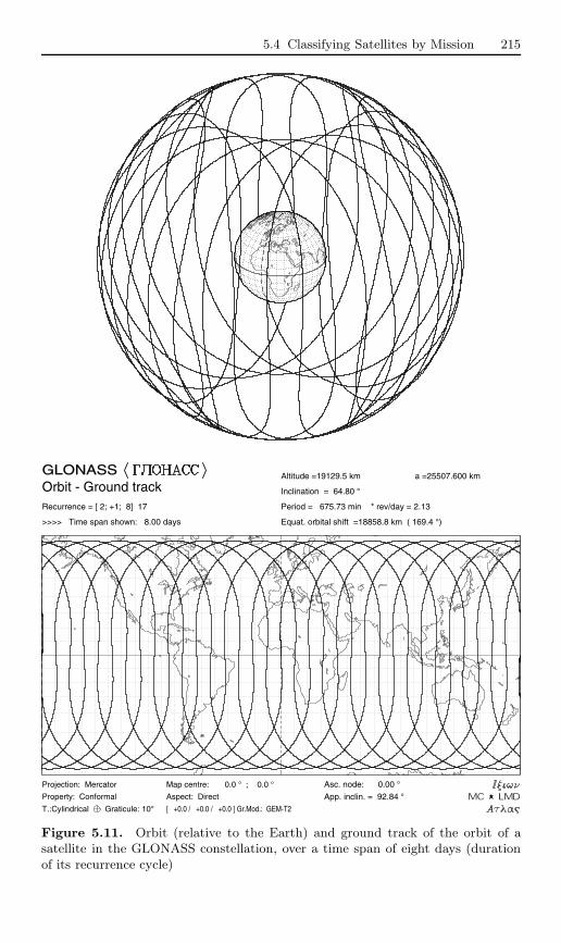
5.4 Classifying Satellites by Mission 215
GLONASSOrbit - Ground trackRecurrence = [ 2; +1; 8] 17
>>>> Time span shown: 8.00 days
Altitude =19129.5 km a =25507.600 km
Inclination = 64.80 °
Period = 675.73 min * rev/day = 2.13
Equat. orbital shift =18858.8 km ( 169.4 °)
Asc. node: 0.00 °
App. inclin. = 92.84 °
Projection: Mercator
Property: Conformal
T.:Cylindrical Graticule: 10°
Map centre: 0.0 ° ; 0.0 °
Aspect: Direct
[ +0.0 / +0.0 / +0.0 ] Gr.Mod.: GEM-T2
Figure 5.11. Orbit (relative to the Earth) and ground track of the orbit of asatellite in the GLONASS constellation, over a time span of eight days (durationof its recurrence cycle)
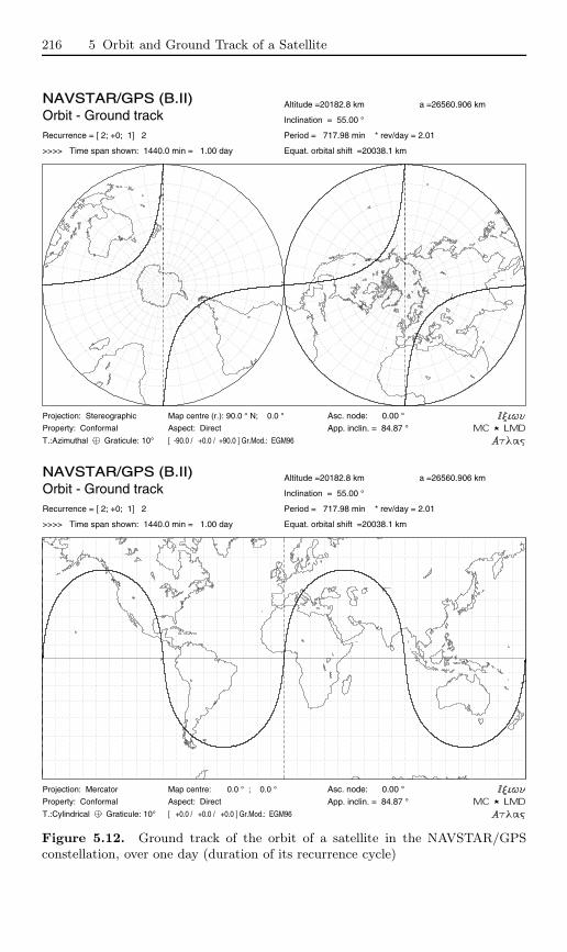
216 5 Orbit and Ground Track of a Satellite
NAVSTAR/GPS (B.II)Orbit - Ground trackRecurrence = [ 2; +0; 1] 2
>>>> Time span shown: 1440.0 min = 1.00 day
Altitude =20182.8 km a =26560.906 km
Inclination = 55.00 °
Period = 717.98 min * rev/day = 2.01
Equat. orbital shift =20038.1 km
Asc. node: 0.00 °
App. inclin. = 84.87 °
Projection: Stereographic
Property: Conformal
T.:Azimuthal Graticule: 10°
Map centre (r.): 90.0 ° N; 0.0 °
Aspect: Direct
[ -90.0 / +0.0 / +90.0 ] Gr.Mod.: EGM96
NAVSTAR/GPS (B.II)Orbit - Ground trackRecurrence = [ 2; +0; 1] 2
>>>> Time span shown: 1440.0 min = 1.00 day
Altitude =20182.8 km a =26560.906 km
Inclination = 55.00 °
Period = 717.98 min * rev/day = 2.01
Equat. orbital shift =20038.1 km
Asc. node: 0.00 °
App. inclin. = 84.87 °
Projection: Mercator
Property: Conformal
T.:Cylindrical Graticule: 10°
Map centre: 0.0 ° ; 0.0 °
Aspect: Direct
[ +0.0 / +0.0 / +0.0 ] Gr.Mod.: EGM96
Figure 5.12. Ground track of the orbit of a satellite in the NAVSTAR/GPSconstellation, over one day (duration of its recurrence cycle)
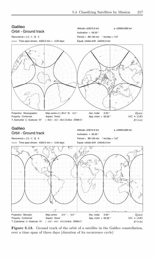
5.4 Classifying Satellites by Mission 217
GalileoOrbit - Ground trackRecurrence = [ 2; -1; 3] 5
>>>> Time span shown: 4320.0 min = 3.00 days
Altitude =23615.6 km a =29993.689 km
Inclination = 56.00 °
Period = 861.58 min * rev/day = 1.67
Equat. orbital shift =24045.0 km
Asc. node: 0.00 °
App. inclin. = 92.82 °
Projection: Stereographic
Property: Conformal
T.:Azimuthal Graticule: 10°
Map centre (r.): 90.0 ° N; 0.0 °
Aspect: Direct
[ -90.0 / +0.0 / +90.0 ] Gr.Mod.: GRIM5-C1
GalileoOrbit - Ground trackRecurrence = [ 2; -1; 3] 5
>>>> Time span shown: 4320.0 min = 3.00 days
Altitude =23615.6 km a =29993.689 km
Inclination = 56.00 °
Period = 861.58 min * rev/day = 1.67
Equat. orbital shift =24045.0 km
Asc. node: 0.00 °
App. inclin. = 92.82 °
Projection: Mercator
Property: Conformal
T.:Cylindrical Graticule: 10°
Map centre: 0.0 ° ; 0.0 °
Aspect: Direct
[ +0.0 / +0.0 / +0.0 ] Gr.Mod.: GRIM5-C1
Figure 5.13. Ground track of the orbit of a satellite in the Galileo constellation,over a time span of three days (duration of its recurrence cycle)

218 5 Orbit and Ground Track of a Satellite
Russian system was constructed using the Tsikada and Nadezhda constella-tions of satellites in polar orbit h = 1 000 km, i = 82.9, such as Kosmos-1383,launched in 1982 or Nadezhda-5 in 1998.
Results of astonishing accuracy (positioning to within a few metres)are currrently obtained with MEO satellite constellations. For the US sys-tem known as NAVSTAR/GPS (Navigation System with Timing and Rang-ing/Global Positioning System), the circular orbit at h = 20 200 km is suchthat the period is 12 hr, or more exactly, half a sidereal day. Satellites in BlockI were experimental, with i = 63, from NAVSTAR-1 (OPS/5111) in 1978 toNAVSTAR-11 (USA-10) in 1985. Block II comprises 24 satellites in 6 planesof 4 operational satellites, with i = 55 (see Figure 5.12), from NAVSTAR-13(USA-35) in 1989 to NAVSTAR-36 (USA-100), launched on 10 March 1994,at which date the system became operational. To replace defective satellites,so-called Block IIR satellites have been launched on a regular basis since1996, such as NAVSTAR-37 (USA-117). By the end of 2004, NAVSTAR-55(USA-178 or GPS-2R-12)) had been reached.
The underlying principle of GPS is simple. Each of the 24 satellites isequipped with a very accurate clock,62 synchronised from a ground station,and a transmitter which sends the clock signal and satellite position, calcu-lated to great accuracy and regularly adjusted. An arbitrary point, whichcan be on the Earth, an aircraft or a satellite, equipped with a receiver candetermine its distance from the emitting satellite by measuring the journeytime of the signal. Since the position of the emitting satellite is known, thistherefore determines a sphere, centred on the satellite, on which the givenpoint must be located. The intersection of this sphere with a second, centredon another satellite, specifies a circle, and the intersection of this circle withyet another sphere, centred on a third satellite, specifies two points. Oneof these two points is an impossible position. A fourth intersecting spherecan confirm this. But the real need for this fourth satellite is to correct thetime measurement made by the receiver clock. Indeed, this clock, paid for bythe user, is a much cheaper one and hence also much less accurate than thetransmitter clock.
The selective availability policy, introduced by the military to limit theaccuracy of the system for civilian activities, was abolished in May 2000. Po-sition determinations are constantly being refined by technological advances,such as more powerful signals and better correction for atmospheric pertur-62 Block II satellites each have caesium and rubidium clocks. Those in Block IIR
should each carry a hydrogen maser atomic clock, with deviation less than 10−14 severy three hours.
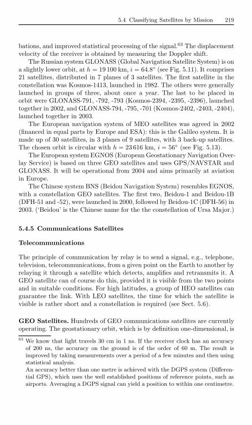
5.4 Classifying Satellites by Mission 219
bations, and improved statistical processing of the signal.63 The displacementvelocity of the receiver is obtained by measuring the Doppler shift.
The Russian system GLONASS (Global Navigation Satellite System) is ona slightly lower orbit, at h = 19 100 km, i = 64.8 (see Fig. 5.11). It comprises21 satellites, distributed in 7 planes of 3 satellites. The first satellite in theconstellation was Kosmos-1413, launched in 1982. The others were generallylaunched in groups of three, about once a year. The last to be placed inorbit were GLONASS-791, -792, -793 (Kosmos-2394, -2395, -2396), launchedtogether in 2002, and GLONASS-794, -795, -701 (Kosmos-2402, -2403, -2404),launched together in 2003.
The European navigation system of MEO satellites was agreed in 2002(financed in equal parts by Europe and ESA): this is the Galileo system. It ismade up of 30 satellites, in 3 planes of 9 satellites, with 3 back-up satellites.The chosen orbit is circular with h = 23 616 km, i = 56 (see Fig. 5.13).
The European system EGNOS (European Geostationary Navigation Over-lay Service) is based on three GEO satellites and uses GPS/NAVSTAR andGLONASS. It will be operational from 2004 and aims primarily at aviationin Europe.
The Chinese system BNS (Beidou Navigation System) resembles EGNOS,with a constellation GEO satellites. The first two, Beidou-1 and Beidou-1B(DFH-51 and -52), were launched in 2000, followed by Beidou-1C (DFH-56) in2003. (‘Beidou’ is the Chinese name for the the constellation of Ursa Major.)
5.4.5 Communications Satellites
Telecommunications
The principle of communication by relay is to send a signal, e.g., telephone,television, telecommunications, from a given point on the Earth to another byrelaying it through a satellite which detects, amplifies and retransmits it. AGEO satellite can of course do this, provided it is visible from the two pointsand in suitable conditions. For high latitudes, a group of HEO satellites canguarantee the link. With LEO satellites, the time for which the satellite isvisible is rather short and a constellation is required (see Sect. 5.6).
GEO Satellites. Hundreds of GEO communications satellites are currentlyoperating. The geostationary orbit, which is by definition one-dimensional, is63 We know that light travels 30 cm in 1 ns. If the receiver clock has an accuracy
of 200 ns, the accuracy on the ground is of the order of 60 m. The result isimproved by taking measurements over a period of a few minutes and then usingstatistical analysis.An accuracy better than one metre is achieved with the DGPS system (Differen-tial GPS), which uses the well established positions of reference points, such asairports. Averaging a DGPS signal can yield a position to within one centimetre.
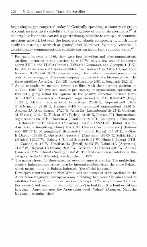
220 5 Orbit and Ground Track of a Satellite
beginning to get congested today.64 Generally speaking, a country or groupof countries sets up its satellite at the longitude of one of its meridians.65 Acountry like Indonesia can use a geostationary satellite to set up a telecommu-nications network between the hundreds of islands composing it, much moreeasily than using a network at ground level. Moreover, for many countries, ageostationary communications satellite has an important symbolic value.66
64 For example, even in 1989, there were four television and telecommunicationssatellites operating at the position λS = 19W, only a few tens of kilometresapart: TDF-1 and TDF-2 (France), TVSat-2 (Germany), and Olympus-1 (UK).In 1999, there were eight Astra satellites, from Astra-1A to Astra-1H, operatingbetween 19.2E and 19.3E, dispensing eight bouquets of television programmesover the same regions. The same company duplicates this achievement with thethree satellites Astra-2A, -2B, -2D, operating since 2001 at longitude 28.2E.
65 As an example, we mention several satellites with their parking position on30 June 1999. We give one satellite per country or organisation, operating atthis date, going round the equator in the positive direction: Sirius-2 (Swe-den) 4.83E, Eutelsat-W3 (European organisation) 7.01E, Italsat-F2 (Italy)16.24E, AfriStar (international foundation) 20.98E, Kopernikus-3 [DFS-3] (Germany) 23.50E, Inmarsat-3-F5 (international organisation) 25.07E,Arabsat-3A (Arab League) 27.20E, Astra-2A (Luxembourg) 28.23E, Gorizont-31 (Russia) 39.91E, Turksat-1C (Turkey) 41.99E, Intelsat-704 (internationalorganisation) 66.04E, Thaicom-3 (Thailand) 78.50E, Zhongwei-1 [Chinastar-1] (China) 87.53E, Measat-1 (Malaysia) 91.49E, INSAT-2C (India) 93.49E,AsiaSat-3S (Hong-Kong/China) 105.50E, Cakrawarta-1 [Indostar-1] (Indone-sia) 107.65E, Mugunghwa-2 [Koreasat-2] (South Korea) 115.89E, N-Star-B (Japan) 133.98E, Optus-A3 [AusSat-3] (Australia) 164.05E, Solidaridad-2(Mexico) 113.00W, Galaxy-8 (United States) 94.94W, Nimiq-1 [Telesat-DTH-1] (Canada) 91.16W, Brasilsat-B3 (Brazil) 84.05W, Nahuel-1A (Argentina)71.87W, Hispasat-1B (Spain) 29.99W, Telecom-2D (France) 5.03W, Amos-1(Israel) 4.03W, Thor-3 (Norway) 0.84W. The first commercial satellite in thiscategory, Anik-A1 (Canada), was launched in 1972.
66 The names chosen for these satellites serve to demonstrate this. The multiethniccountry Indonesia, sometimes torn by internal conflict, chose the name Palapa,which means ‘unity’ in Bahasa Indonesia (the official language).Developed countries in the New World seek the names of their satellites in theAmerindian languages, perhaps as a way of finding their roots. Canada named itssatellites Anik (, in Inuit writing) and Nimiq (ς), which means ‘brother’(for a sister) and ‘union’ (or ‘bond that unites’) in Inuktitut (the Inuit or Eskimolanguage). Argentina uses the Araucanian word ‘Nahuel’ (Araucan, Mapuchelanguage), meaning ‘tiger’.
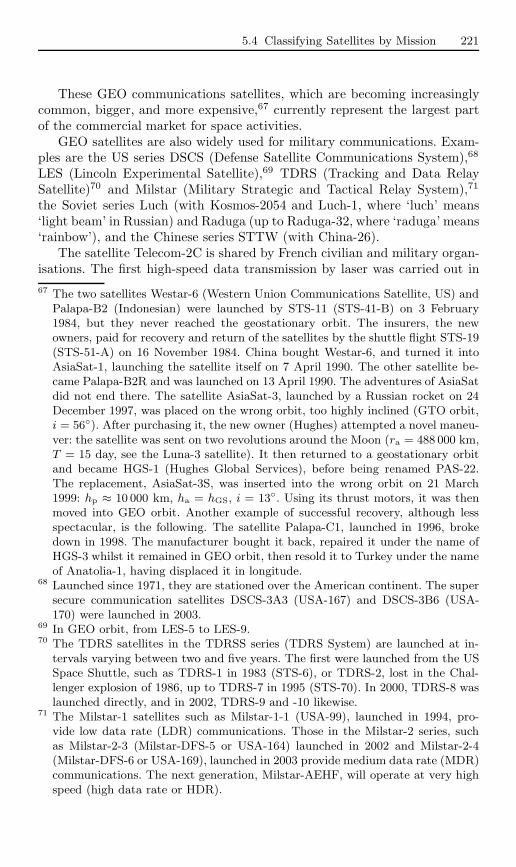
5.4 Classifying Satellites by Mission 221
These GEO communications satellites, which are becoming increasinglycommon, bigger, and more expensive,67 currently represent the largest partof the commercial market for space activities.
GEO satellites are also widely used for military communications. Exam-ples are the US series DSCS (Defense Satellite Communications System),68
LES (Lincoln Experimental Satellite),69 TDRS (Tracking and Data RelaySatellite)70 and Milstar (Military Strategic and Tactical Relay System),71
the Soviet series Luch (with Kosmos-2054 and Luch-1, where ‘luch’ means‘light beam’ in Russian) and Raduga (up to Raduga-32, where ‘raduga’ means‘rainbow’), and the Chinese series STTW (with China-26).
The satellite Telecom-2C is shared by French civilian and military organ-isations. The first high-speed data transmission by laser was carried out in67 The two satellites Westar-6 (Western Union Communications Satellite, US) and
Palapa-B2 (Indonesian) were launched by STS-11 (STS-41-B) on 3 February1984, but they never reached the geostationary orbit. The insurers, the newowners, paid for recovery and return of the satellites by the shuttle flight STS-19(STS-51-A) on 16 November 1984. China bought Westar-6, and turned it intoAsiaSat-1, launching the satellite itself on 7 April 1990. The other satellite be-came Palapa-B2R and was launched on 13 April 1990. The adventures of AsiaSatdid not end there. The satellite AsiaSat-3, launched by a Russian rocket on 24December 1997, was placed on the wrong orbit, too highly inclined (GTO orbit,i = 56). After purchasing it, the new owner (Hughes) attempted a novel maneu-ver: the satellite was sent on two revolutions around the Moon (ra = 488 000 km,T = 15 day, see the Luna-3 satellite). It then returned to a geostationary orbitand became HGS-1 (Hughes Global Services), before being renamed PAS-22.The replacement, AsiaSat-3S, was inserted into the wrong orbit on 21 March1999: hp ≈ 10 000 km, ha = hGS, i = 13. Using its thrust motors, it was thenmoved into GEO orbit. Another example of successful recovery, although lessspectacular, is the following. The satellite Palapa-C1, launched in 1996, brokedown in 1998. The manufacturer bought it back, repaired it under the name ofHGS-3 whilst it remained in GEO orbit, then resold it to Turkey under the nameof Anatolia-1, having displaced it in longitude.
68 Launched since 1971, they are stationed over the American continent. The supersecure communication satellites DSCS-3A3 (USA-167) and DSCS-3B6 (USA-170) were launched in 2003.
69 In GEO orbit, from LES-5 to LES-9.70 The TDRS satellites in the TDRSS series (TDRS System) are launched at in-
tervals varying between two and five years. The first were launched from the USSpace Shuttle, such as TDRS-1 in 1983 (STS-6), or TDRS-2, lost in the Chal-lenger explosion of 1986, up to TDRS-7 in 1995 (STS-70). In 2000, TDRS-8 waslaunched directly, and in 2002, TDRS-9 and -10 likewise.
71 The Milstar-1 satellites such as Milstar-1-1 (USA-99), launched in 1994, pro-vide low data rate (LDR) communications. Those in the Milstar-2 series, suchas Milstar-2-3 (Milstar-DFS-5 or USA-164) launched in 2002 and Milstar-2-4(Milstar-DFS-6 or USA-169), launched in 2003 provide medium data rate (MDR)communications. The next generation, Milstar-AEHF, will operate at very highspeed (high data rate or HDR).
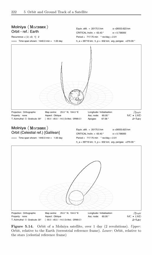
222 5 Orbit and Ground Track of a Satellite
MolniyaOrbit - ref.: EarthRecurrence = [ 2; +0; 1] 2
>>>> Time span shown: 1440.0 min = 1.00 day
Equiv. altit. = 20175.5 km
e = 0.736000
a =26553.623 km
CRITICAL Inclin. = 63.43 °
Period = 717.75 min * rev/day = 2.01
h_a = 39719 km; h_p = 632 km; arg. perigee: +270.00 °
Longitude / Initialisation:
Asc. node: 60.00 °
Apogee: 67.06 °
Projection: Orthographic
Property: none
T.:Azimuthal Graticule: 30°
Map centre: 25.0 ° N; 104.0 °E
Aspect: Oblique
[ -90.0 / +65.0 / -14.0 ] Gr.Mod.: GRIM5-C1
MolniyaOrbit (Celestial ref.) [Galilean]>>>> Time span shown: 1440.0 min = 1.00 day
Equiv. altit. = 20175.5 km
e = 0.736000
a =26553.623 km
CRITICAL Inclin. = 63.43 °
Period = 717.75 min * rev/day = 2.01
h_a = 39719 km; h_p = 632 km; arg. perigee: +270.00 °
Longitude / Initialisation:
Asc. node: 60.00 °
Projection: Orthographic
Property: none
T.:Azimuthal Graticule: 30°
Map centre: 25.0 ° N; 104.0 °E
Aspect: Oblique
[ -90.0 / +65.0 / -14.0 ] Gr.Mod.: GRIM5-C1
Figure 5.14. Orbit of a Molniya satellite, over 1 day (2 revolutions). Upper :Orbit, relative to the Earth (terrestrial reference frame). Lower : Orbit, relative tothe stars (celestial reference frame)
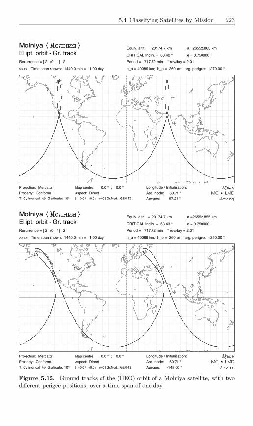
5.4 Classifying Satellites by Mission 223
MolniyaEllipt. orbit - Gr. trackRecurrence = [ 2; +0; 1] 2
>>>> Time span shown: 1440.0 min = 1.00 day
Equiv. altit. = 20174.7 km
e = 0.750000
a =26552.863 km
CRITICAL Inclin. = 63.42 °
Period = 717.72 min * rev/day = 2.01
h_a = 40089 km; h_p = 260 km; arg. perigee: +270.00 °
Longitude / Initialisation:
Asc. node: 60.71 °
Apogee: 67.24 °
Projection: Mercator
Property: Conformal
T.:Cylindrical Graticule: 10°
Map centre: 0.0 ° ; 0.0 °
Aspect: Direct
[ +0.0 / +0.0 / +0.0 ] Gr.Mod.: GEM-T2
MolniyaEllipt. orbit - Gr. trackRecurrence = [ 2; +0; 1] 2
>>>> Time span shown: 1440.0 min = 1.00 day
Equiv. altit. = 20174.7 km
e = 0.750000
a =26552.855 km
CRITICAL Inclin. = 63.43 °
Period = 717.72 min * rev/day = 2.01
h_a = 40089 km; h_p = 260 km; arg. perigee: +250.00 °
Longitude / Initialisation:
Asc. node: 60.71 °
Apogee: -148.00 °
Projection: Mercator
Property: Conformal
T.:Cylindrical Graticule: 10°
Map centre: 0.0 ° ; 0.0 °
Aspect: Direct
[ +0.0 / +0.0 / +0.0 ] Gr.Mod.: GEM-T2
Figure 5.15. Ground tracks of the (HEO) orbit of a Molniya satellite, with twodifferent perigee positions, over a time span of one day

224 5 Orbit and Ground Track of a Satellite
TundraEllipt. orbit - Gr. trackRecurrence = [ 1; +0; 1] 1
>>>> Time span shown: 1440.0 min = 1.00 day
Equiv. altit. = 35785.2 km
e = 0.266800
a =42163.383 km
CRITICAL Inclin. = 63.43 °
Period = 1436.04 min * rev/day = 1.00
h_a = 47034 km; h_p =24536 km; arg. perigee: +270.00 °
Longitude / Initialisation:
Asc. node: -69.80 °
Apogee: -100.00 °
Projection: Orthographic
Property: none
T.:Azimuthal Graticule: 10°
Map centre: 15.0 ° N; 95.0 ° W
Aspect: Oblique
[ -90.0 / +75.0 / -175.0 ] Gr.Mod.: GEM-T2
SupertundraEllipt. orbit - Gr. trackRecurrence = [ 1; +0; 1] 1
>>>> Time span shown: 1440.0 min = 1.00 day
Equiv. altit. = 35785.1 km
e = 0.423000
a =42163.191 km
CRITICAL Inclin. = 63.43 °
Period = 1436.03 min * rev/day = 1.00
h_a = 53620 km; h_p =17950 km; arg. perigee: +270.00 °
Longitude / Initialisation:
Asc. node: -63.02 °
Apogee: -110.00 °
Projection: Orthographic
Property: none
T.:Azimuthal Graticule: 10°
Map centre: 15.0 ° N; 105.0 ° W
Aspect: Oblique
[ -90.0 / +75.0 / -165.0 ] Gr.Mod.: GEM-T2
Figure 5.16. Ground tracks of satellites in (HEO) Tundra and Supertundra orbits,over a time span of one day

5.4 Classifying Satellites by Mission 225
LoopusEllipt. orbit - Gr. trackRecurrence = [ 2; -1; 3] 5
>>>> Time span shown: 4320.0 min = 3.00 days
Equiv. altit. = 23613.3 km
e = 0.600000
a =29991.445 km
CRITICAL Inclin. = 63.43 °
Period = 861.53 min * rev/day = 1.67
h_a = 41608 km; h_p = 5618 km; arg. perigee: +270.00 °
Longitude / Initialisation:
Asc. node: 2.61 °
Apogee: 0.00 °
Projection: Orthographic
Property: none
T.:Azimuthal Graticule: 10°
Map centre (r.): 45.0 ° N; 36.0 °E
Aspect: Oblique
[ -90.0 / +45.0 / +54.0 ] Gr.Mod.: GEM-T2
LoopusEllipt. orbit - Gr. trackRecurrence = [ 2; -1; 3] 5
>>>> Time span shown: 4320.0 min = 3.00 days
Equiv. altit. = 23613.3 km
e = 0.600000
a =29991.445 km
CRITICAL Inclin. = 63.43 °
Period = 861.53 min * rev/day = 1.67
h_a = 41608 km; h_p = 5618 km; arg. perigee: +270.00 °
Longitude / Initialisation:
Asc. node: 2.61 °
Apogee: 0.00 °
Projection: Mercator
Property: Conformal
T.:Cylindrical Graticule: 10°
Map centre: 0.0 ° ; 0.0 °
Aspect: Direct
[ +0.0 / +0.0 / +0.0 ] Gr.Mod.: GEM-T2
Figure 5.17. Ground track of the (HEO) orbit of a satellite in the Loopus con-stellation, over a time span of three days
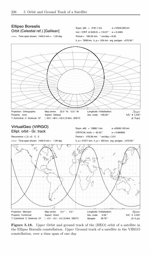
226 5 Orbit and Ground Track of a Satellite
Ellipso BorealisOrbit (Celestial ref.) [Galilean]>>>> Time span shown: 1440.0 min = 1.00 day
Equiv. altit. = 4181.1 km
e = 0.3463
a =10559.260 km
Incl. / CRIT. & SUN-S. = 116.57 °
Period = 180.00 min * rev/day = 8.00
h_a = 7838 km; h_p = 524 km; arg. perigee: +270.00 °
Longitude / Initialisation:
Asc. node: -100.00 °
Projection: Orthographic
Property: none
T.:Azimuthal Graticule: 10°
Map centre: 22.0 ° N; 12.0 ° W
Aspect: Oblique
[ -90.0 / +68.0 / +102.0 ] Gr.Mod.: GEM-T2
VirtualGeo (VIRGO)Ellipt. orbit - Gr. trackRecurrence = [ 3; +0; 1] 3
>>>> Time span shown: 1440.0 min = 1.00 day
Equiv. altit. = 13882.1 km
e = 0.660850
a =20260.193 km
CRITICAL Inclin. = 63.42 °
Period = 478.36 min * rev/day = 3.01
h_a = 27271 km; h_p = 493 km; arg. perigee: +270.00 °
Longitude / Initialisation:
Asc. node: 0.00 °
Apogee: 36.78 °
Projection: Mercator
Property: Conformal
T.:Cylindrical Graticule: 10°
Map centre: 0.0 ° ; 0.0 °
Aspect: Direct
[ +0.0 / +0.0 / +0.0 ] Gr.Mod.: GEM-T2
Figure 5.18. Upper Orbit and ground track of the (HEO) orbit of a satellite inthe Ellipso Borealis constellation. Upper Ground track of a satellite in the VIRGOconstellation, over a time span of one day
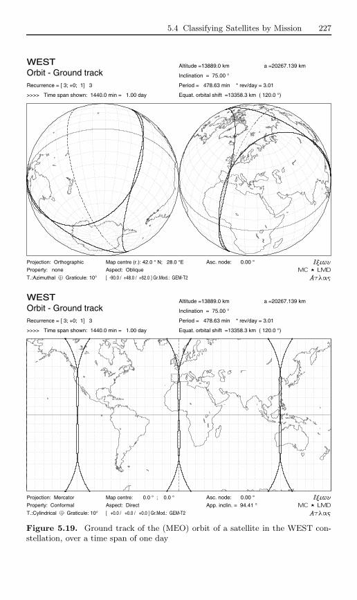
5.4 Classifying Satellites by Mission 227
WESTOrbit - Ground trackRecurrence = [ 3; +0; 1] 3
>>>> Time span shown: 1440.0 min = 1.00 day
Altitude =13889.0 km a =20267.139 km
Inclination = 75.00 °
Period = 478.63 min * rev/day = 3.01
Equat. orbital shift =13358.3 km ( 120.0 °)
Asc. node: 0.00 °Projection: Orthographic
Property: none
T.:Azimuthal Graticule: 10°
Map centre (r.): 42.0 ° N; 28.0 °E
Aspect: Oblique
[ -90.0 / +48.0 / +62.0 ] Gr.Mod.: GEM-T2
WESTOrbit - Ground trackRecurrence = [ 3; +0; 1] 3
>>>> Time span shown: 1440.0 min = 1.00 day
Altitude =13889.0 km a =20267.139 km
Inclination = 75.00 °
Period = 478.63 min * rev/day = 3.01
Equat. orbital shift =13358.3 km ( 120.0 °)
Asc. node: 0.00 °
App. inclin. = 94.41 °
Projection: Mercator
Property: Conformal
T.:Cylindrical Graticule: 10°
Map centre: 0.0 ° ; 0.0 °
Aspect: Direct
[ +0.0 / +0.0 / +0.0 ] Gr.Mod.: GEM-T2
Figure 5.19. Ground track of the (MEO) orbit of a satellite in the WEST con-stellation, over a time span of one day
228 5 Orbit and Ground Track of a Satellite
2001 between the European GEO satellite Artemis, launched just before forthis purpose, and the French LEO satellite SPOT-4. This prefigured trans-missions between LEO satellites via a GEO satellite as intermediary.
HEO Satellites. The most common HEO orbit is the one used by So-viet then Russian satellites, the Molniya orbit (meaning ‘lightning’), sinceKosmos-41 in 1964. The number of satellites launched in these orbits is stag-gering: 93 for Molniya-1, from Molniya-1-01 in 1965 to Molniya-1-91 in 1998,then Molniya-1-92 in 2003 and Molniya-1-93 (Kosmos-2405) in 2004, 17 forMolniya-2, from Molniya-2-01 in 1971 to Molniya-2-17 in 1977, 53 for thepresent series Molniya-3, from Molniya-3-01 in 1974 to Molniya-3-53 in 2003.
The satellites in these three series have the same orbit, to within a few tensof kilometres:72 hp ≈ 500 km, ha ≈ 40 000 km, i = 63 (critical inclination).The period is 12 hr (half a sidereal day): T = 717.7 min, a = 26 553 km,e between 0.72 and 0.75. The argument of the perigee is ω = −90, whichmeans that the perigee is located in the southern hemisphere, region of theEarth that the satellite overflies very quickly (see Example 1.3). On the otherhand, at the apogee, the satellite is almost stationary for 8 hr, when aboveRussia (see Example 5.7). The orbit and the ground track of this orbit areshown in Fig. 5.14 and 5.15.
This orbit is at the critical inclination, which fixes the position of theperigee (and the apogee). Furthermore, the orbit is recurrent with a cycle ofone day: the ground track passes through the same point every day. Withthree regularly spaced satellites on the same orbit, one almost achieves theequivalent of a geostationary satellite for the regions close to the ground trackat apogee. This is a judicious method for solving the problem of geosyn-chronicity at high latitudes.
The US military satellites SDS (Space Defense System), from SDS-1 in1976 to SDS-7 (USA-21) in 1987, are in Molniya orbit.
The Tundra and Supertundra orbits, shown in Fig. 5.16 and discussedin Chap. 4, are far less commonly used. The constellation SD-Radio, whichprovides radio transmissions for American road users, is in a Tundra orbit.The perigee of these two orbits is high, well above the Van Allen radiationbelt. This is not so for the Molniya orbits, where satellites cross this belt onevery revolution, an ordeal for electronic equipment.72 As an example, here are the characteristics of several Molniya orbits with the
launch date of the satellite, using the notation [hp/ha/i] (altitudes in km,angle in degrees): Molniya-1-01 (23 April 1965) [538/39300/65.5], Molniya-2-01 (25 November 1971) [516/39553/65.0], Molniya-3-01 (21 March 1974)[250/40095/64.1], Molniya-3-50 (8 July 1999) [464/39889/62.8], Molniya-3-51 (20July 2001) [407/40831/62.9], Molniya-3-52 (25 October 2001) [615/40658/62.9],Molniya-3-53 (19 June 2003) [637/39709/62.8], Molniya-1-93 (18 February 2004)[634/39729/62.8].

5.4 Classifying Satellites by Mission 229
The Loopus orbit, a = 30 000 km, e = 0.6, Fig. 5.17, lies outside theradiation belts. The period of the satellite is 3/5 of a day (T = 861.526 min,see Galileo orbital characteristics).
The Ellipso Borealis orbit is highly original, as we have already seen:it is Sun-synchronous and has the critical inclination. The parameters are:hp = 524 km, ha = 7 838 km, i = 116.57, ω = −90, with a period of 3 hr[see Fig. 5.18 (upper) and Colour Plate VII]. The Ellipso project includes aHEO constellation, Borealis, with 10 satellites in 2 planes, and a constellation,Concordia, with 4 (or perhaps 7) satellites in equatorial orbit, h = 8 050 km,i = 0.0.
The US projects COBRA (Communications Orbiting Broadband Re-peating Arrays) and VIRGO (or VirtualGEO, Virtual Geostationary) useHEO orbits with a period of 8 hr, precisely one third of a sidereal day:a = 20 261 km, e = 0.6458, i = 63.4 (see the lower part of Fig. 5.18). As inthe Molniya case, the VIRGO constellation is effectively playing the role ofa geostationary satellite.
MEO Satellites. The WEST orbit is circular with h = 13 900 km, i = 75
and a period of 8 hr (one third of a sidereal day), Fig. 5.19. The WESTconstellation project (Wideband European Satellite Telecommunication) in-cludes 9 satellites on this MEO orbit, together with 2 GEO satellites.
Satellites Between LEO and MEO. The Odyssey project, abandoned in2000, consisted of a constellation of 3 planes of 4 satellites, h = 10 354 km,i = 50. The ICO constellation (Intermediate Circular Orbit)73 comprises 2planes of 5 satellites, h = 10 390 km, i = 45.
LEO Satellites. Communications using LEO satellites always require a con-stellation. For telephone communications, the advantage of LEO constella-tions is the very short response time: the journey time of the signal transitingvia a GEO satellite is about 250 ms, and this quarter of a second is sometimesconsidered to be a nuisance. However, this is not a big enough advantage toensure the success of a commercial venture. The failure of Iridium74 in 2000and GlobalStar in 2002 clearly demonstrates this. The following satellite con-stellations were operating or under construction (or had failed) in 2004:
• Orbcomm, 35 satellites (3 planes of 8), h = 810 km, i = 45.0,• Iridium, 88 satellites (6 planes of 11), h = 780 km, i = 86.4,• GlobalStar, 52 satellites (8 planes of 6), h = 1 410 km, i = 52.0,
73 Launch date: ICO-F2 on 19 June 2001.74 Faced with commercial failure, the first reaction was to remove all the satellites
from orbit. However, in the end, the system was taken over by the US Departmentof Defense. Originally, the constellation was to include 77 satellites, whence thename Iridium, which is the chemical element (Ir) with atomic number 77.
230 5 Orbit and Ground Track of a Satellite
• Teledesic,75 288 satellites (12 planes of 24), h = 550 km, i = 97.7.
The total number of satellites in each constellation76 includes all spare satel-lites.
The Russian system Gonets-D1 (‘gonets’ means ‘messenger’) is the com-mercial version of the military system Strela-3 (‘strela’ means ‘arrow’). Theconstellation was set up77 with the following characteristics:
• Gonets-D1, 48 satellites (6 planes of 8), h = 1400 km, i = 82.5.
The OSCAR satellites (Orbiting Satellite Carrying Amateur Radio), notto be confused with Transit-Oscar, are launched on a regular basis foramateur radio transmissions. Orbits are often near-polar and LEO, as forOSCAR-1 in 1961 or OSCAR-30 in 1996.
Passive Communication
As their name suggests, the satellites Echo-1 and -2 were launched as passivetelecommunications relays. As one might imagine, the results were not veryconvincing and this experimental system was dropped. However, these twosatellites were originally intended for space geodesy.
We should also mention another attempt to create a passive space com-munications system. The idea was to place a ring in orbit around the Earthto reflect radio waves. This was the US experiment called Westford Needles.Two packages (Westford-1 and -2) were inserted into orbit. Once opened, theydistributed 350 then 475 million small copper needles (1.7 cm long, 0.1 mmin diameter) along their trajectory. These military experiments were carried
75 The original project, in 1994, was to launch 840 active satellites (21 planes of40).
76 Launch dates of the first and last satellite in each constellation: Orbcomm con-stellation: Orbcomm-FM-1 and -FM-2 on 3 April 1995, launched with Microlab-1, h = 740 km, i = 69.9, Orbcomm-FM-3 and -FM-4 on 10 February 1998,launched with GFO-1, h = 830 km, i = 108.0, the other Orbcomm satelliteswere launched with inclination i = 45.0, in clusters of 8, (beginning) Orbcomm-FM-5 to -FM-12 on 23 December 1997, (end) Orbcomm-FM-30 to -FM-36 on4 December 1999. Iridium constellation: (beginning) Iridium-4 to -8 on 5 May1997, (end of initial programme) Iridium-83 to -86 on 6 November 1998, (restart)Iridium-90 to -96 on 11 February 2002, Iridium-97 and -98 on 20 June 2002. Glob-alStar constellation: (beginning) GlobalStar-M001 to -M004 on 14 February 1998,(end) GlobalStar-M061 to -M064 on 4 December 1999. Teledesic constellation:(demonstration satellite) Teledesic-1 on 26 February 1998.
77 The Strela-3 satellites were launched in clusters of 6. With the establishment ofthe Gonets-D1 constellation, each cluster of 6 satellites has included 3 militaryand 3 civilian. Launch dates: Gonets-D1-1, -2 and -3 (with the Strela-3 satellites,Kosmos-2328, -2329, -2330) on 19 February 1996, Gonets-D1-4 and the followingon 14 February 1997, Gonets-D1-7 and the following on 17 December 2001.
5.4 Classifying Satellites by Mission 231
out between 1961 and 1963, from the satellites MIDAS-4, -5 and -7, in cir-cular near-polar orbit h = 3 600 km. They were called Westford-1, WestfordDrag, and Westford-2, respectively. The experiment was severely criticisedby astronomers who saw in this a source of optical and radio pollution. Inthe end, the needles constituted neither a reflector nor a pollutant.
5.4.6 Satellites for Fundamental Physics
The satellite Gravity Probe-B (GP-B), launched on 20 April 2004, has astrictly polar LEO orbit, already mentioned in the last chapter. Its groundtrack is illustrated in the lower part of Fig. 5.5. The aim of the mission is tomeasure, using gyroscopes, the extent to which space and time are distortedby the presence of the Earth, within the framework of the general theory ofrelativity. The preliminary experiment GP-A, in June 1976, sent a hydrogenmaser clock into space in a sub-orbital flight up to an altitude of 10 000 km.
Two missions are being planned to provide experimental corroboration forthe principle of equivalence.78 The French project µSCOPE (Micro-Satellitea Compensation de Traınee pour l’Observation du Principe d’Equivalence),or Microscope, is designed to check the universality of free fall. The satellitewill have a circular, Sun-synchronous LEO orbit at h ≈ 700 km. Drag ef-fects on the satellite will be compensated by electric thrusters to ensure thatthe two test masses carried aboard undergo perfect free-fall conditions overthousands of kilometers (rather than just a few tens of meters, and with-out compensation for air resistance, if one drops the objects from the leaningtower of Pisa). The US satellite STEP (Satellite Test of the Equivalence Prin-ciple) will be much bigger, with cooled instruments to increase measurementaccuracy.79 It will also follow a circular LEO orbit, with h = 400 km.
The LISA project (Laser Interferometer Space Antenna), a joint venturebetween NASA and ESA, will attempt to detect gravitational waves usingthree satellites in formation on a heliocentric orbit.80
78 The principle of equivalence postulated by Einstein is based on the observationthat all bodies, independently of their mass, have the same acceleration in agravitational field for identical initial conditions. This is the universal principleof free fall: the passive gravitational mass of a body (m = mg in the expressionfor the gravitational force, involving G) is equal to the inertial mass (m = mi inNewton’s second law).
79 The relation mg/mi = 1 has been checked on Earth to an accuracy of 10−12.The µSCOPE experiment aims to achieve 10−14 and STEP 10−17.
80 The three satellites will be placed at the corners of an equilateral triangle withside 5 million kilometres. The centre of the triangle will lie in the plane of theecliptic at a distance of 1 a.u. from the Sun. The angle between the centre of thetriangle, the Sun and the Earth will be equal to 20 (measured positively). Thethree satellites, linked by laser, will constitute a gigantic Michelson interferom-eter.
232 5 Orbit and Ground Track of a Satellite
5.4.7 Satellites for Astronomy and Astrophysics
Astronomy and Astrometry
In most cases, astronomical missions are one-off experiments and the satellitesare not systematically placed on the same orbits, as they might be for remote-sensing, for example. We shall discuss here several satellites for each region ofthe electromagnetic spectrum used in astronomy. Most of them are Americanand the remainder are mainly European. NASA launched a programme oflarge orbiting observatories (Great Observatories Program): GRO (GammaRay Observer), renamed Compton,81 for γ rays, AXAF (Advanced X-rayAstrophysics Facility), renamed Chandra,82 for X rays, HST (Hubble SpaceTelescope) often called Hubble83 for the visible, and SIRTF (Space InfraRedTelescope Facility) renamed84 Spitzer or SST (Spitzer Space Telescope) afterlaunch, for the infrared.
Concerning more modest missions, the Explorer programme is NASA’scontinuing programme for orbital astronomy and space physics packages.Explorers come in three sizes defined by budget considerations: MediumExplorer (MIDEX), Small Explorer (SMEX), and University-class Explorer(UNEX).
Cosmic Rays, Gamma Rays. Gamma astronomy began in 1961 withExplorer-11, hp = 480 km, ha = 1 460 km, i = 29, which provided thefirst detection of gamma rays from space. This was followed by OSO-3 andOSO-7, both on the orbit h = 550 km, i = 33, then Explorer-48 (SAS-2),h = 526 km, i = 1, not forgetting the Vela satellites mentioned again below.
In this field of investigation, orbits are generally low and not highly in-clined, as for the HEAO satellites (High Energy Astrophysical Observatory),HEAO-1, -2 (renamed Einstein), -3, h ≈ 500 km, i = 23, 23 and 44,81 Arthur Holly Compton (1892–1962) was an American physicist. His work on X
rays led him to discover in 1923 the effect which now carries his name (interactionbetween matter and X rays). He also studied cosmic rays.
82 Subrahmanyan Chandrasekhar (1910–1995) was an American astrophysicist ofIndian birth. He carried out a great many theoretical studies on the internalstructure of stars. He studied radiative transfer in stellar atmospheres. The root‘chand’ means ‘Moon’ or ‘bright’ in Sanskrit.
83 Edwin Powell Hubble (1889–1953) was an American astronomer. He produced aclassification of extragalactic nebulas and, in 1928, established the law of spectralshifts now known as the Hubble law, which says that the spectral shift of a galaxy(redshift) is proportional to its distance, thus confirming the hypothesis that theUniverse is expanding. The constant of proportionality H0, called the Hubbleconstant, is not precisely known and may even vary in time. It is measured inkms−1 per megaparsec. Its reciprocal, which has units of time, gives the age ofthe Universe to within an order of magnitude: 1/H0 ≈ 10 billion years.
84 In honour of Lyman Spitzer Jr. (1914–1957), the American astrophysicist whowas the first to suggest placing a large telescope in space.
5.4 Classifying Satellites by Mission 233
or the HETE satellites (High Energy Transient Experiment), HETE-1, -2,h ≈ 500 km, i = 38 and 2. The Compton satellite (also called CGRO),launched on 5 April 1991 by STS-37, h = 450 km, i = 28.5, had a massof 15 tonnes, of which 7 tonnes represented instrumentation. Great precau-tions were taken when it was de-orbited on 3 June 2000. The internationalproject GLAST (Gamma-ray Large Area Space Telescope) will use a simi-lar orbit: h = 550 km, i = 28.5, and the Italian Agile satellite will be inequatorial orbit, h = 550 km, i ≈ 0. The US project Swift (MIDEX-3)for detection of gamma-ray bursts will follow a similar orbit, h = 600 km,i = 19. The European satellite Integral (International Gamma-Ray Astro-physics Laboratory), launched on 17 October 2002, is on an HEO orbit:a = 87 698.656 km, e = 0.8204 (i.e., hp = 9 400 km, ha = 153 300 km),i = 57.1, T = 71.8 hr = 3Jsid,see Fig.5.20 and 5.21 (upper).
X Rays. Certain orbits are like those seen above, i.e., low, with h ≈ 550 km,and with low inclination: i = 53 for ROSAT, i = 4 for BeppoSAX (Satelliteper Astronomia a raggi X ), i = 23 for XTE (X-ray Timing Explorer), i =38 for HESSI (High-Energy Solar Spectroscopic Imager, SMEX-6), renamedRHESSI (Reuven Ramaty HESSI).
The rest are very high and highly eccentric, as in the case of the Sovietsatellites Astron and Granat, or the European satellite Exosat, launched in1983 (one revolution is shown in the upper part of Fig. 5.22). In 1999, twolarge satellites, one American and the other European, used this type oforbit: Chandra (also called CXO, Chandra X-ray Observatory), launched on23 July by STS-93, hp = 10 157 km, ha = 138 672 km, i = 29.0, T = 63.5 hr,and XMM (ESA’s X-ray Multi-Mirror Space Observatory, renamed XMM-Newton), launched on 10 December, hp = 7 417 km, ha = 113 678 km, i =38.8, T = 47.9 hr.
Ultraviolet (UV). These satellites use slightly inclined LEO orbits. Thesatellites OAO-1, -2, -3 (Orbiting Astronomical Observatory), launched be-tween 1966 and 1972, were on the orbit h = 750 km, i = 35. OAO-3was renamed Copernicus to mark the 500th anniversary of the birth of thegreat man. The US satellites EUVE (Extreme UV Explorer), h = 515 km,i = 28.4, FUSE (Far UV Spectroscopic Explorer, MIDEX-0), h = 760 km,i = 25.0, and GALEX (Galaxy Evolution Experiment, SMEX-7), h =690 km, i = 28.0 were launched in 1992, 1999 and 2003, respectively. Theorbit of the Spanish Minisat-01, launched in 1997, h = 570 km, is also tiltedby about thirty degrees to the equator, since i = 151 (which is the highestvalue yet encountered, to our knowledge).
The satellite CHIPSat (Cosmic Hot Interstellar Plasma SpectrometerSatellite, UNEX-1) is on a near-polar orbit since it was launched as a passen-ger of ICESat. CHIPSat was the first US mission to use end-to-end satelliteoperations with TCP/IP and FTP.
234 5 Orbit and Ground Track of a Satellite
Visible. In the visible region of the electromagnetic spectrum, the two largestmissions have been the European Hipparcos and the American Hubble (withESA participation). Both have provided excellent results, despite a difficultstart.
The Hipparcos satellite (High Precision Parallax Collecting Satellite, com-bined with the name of the great Greek astronomer Hipparchos) was devotedto astrometry85 (accurate measurement of stellar positions). Launched on 8August 1989, the satellite did not reach the planned geostationary orbit butinstead remained in the highly eccentric transfer orbit (GTO): hp = 542 km,ha = 35 840 km, i = 6.7. Rewriting the computer programs and redis-tributing the ground receiving stations, the mission was nevertheless carriedsuccessfully to completion.
The Hubble observatory was correctly launched by STS-31 on 24 April1990. The problems began as soon as the first image came through, clearlyshowing that the telescope was shortsighted due to an inexcusable mirrordefect. The intention had been to carry out maintenance via the Shuttle,and this possibility was used primarily to correct the optics. The results didindeed come up to expectations and astronomy was revolutionised in theprocess.
In contrast, Hubble’s successor must be beyond reproach from the mo-ment of launch: NGST (New Generation Space Telescope), renamed86 JWST(James Webb Space Telescope), should be placed at the Lagrange point L2
of the Sun–Earth system (see Sect. 3.14), and it will be quite impossible togo out there and repair it! In addition to the visible region, JWST will alsoobserve in the infrared and for this reason will be equipped with cryogenicsystems. The successor to Hipparcos, named GAIA (Global Astrometric In-terferometer for Astrophysics, with reference to , Gæe or Gaia, thepersonification of the Earth according to the Ancient Greeks) will also beplaced there.87 The main advantage of the halo orbit (L2LO) around thepoint L2 for stellar observation is that the Sun, the Earth and the Moon areall located behind the line of sight of the telescope. The whole of the celestialsphere can then be observed as the year goes by, without blind spots. Thisregion is also very stable as regards the thermal and particle environment.85 The satellite determined the position, luminosity, and distance of 118 218 stars.
The accuracy of the measurements (2 milliarcsec), was 100 times better thanground-based measurements of the day.
86 In honour of James E. Webb (1906–1992), NASA’s second administrator. Hedirected the Apollo programme and was one of the instigators of the first inter-planetary exploration.
87 GAIA’s mission is to observe and record a billion stars with an accuracy of10 µarcsec. For stars within 500 light-years, the distance will then be calculableto within a few light-years.
5.4 Classifying Satellites by Mission 235
Infrared (IR). The detection of IR radiation involves cooling the opticalsystem and associated instrumentation in the satellite. The satellite ceasesto function once its reserves of cryogenic fluid have been exhausted.
Certain satellites have used Sun-synchronous orbits, such as the helium-cooled IRAS (IR All-sky Survey), h = 890 km, launched in 1983, and WIRE(Wide field IR Explorer, SMEX-5), launched in 1999 with h = 560 km, whoseoptical system is cooled by 3 kg of solid hydrogen. The satellite WISE (Widefield IR Survey Explorer, MIDEX-5), h = 600 km, will also be in this typeof orbit.
The European satellite ISO (Infrared Space Observatory), with Americanand Japanese participation, was equipped with a cryostat filled with super-fluid helium. It operated between November 1995 and May 1998 on a highlyeccentric orbit, with a period of revolution of one day.88 Its successor Her-schel89 (or HSO, Herschel Space Observatory), taking over from the FIRSTproject (Far IR and Submillimeter Telescope), will be placed in orbit aroundthe Lagrange point L2, for three years. JASMINE (Japan Astrometry Satel-lite Mission for Infrared Exploration) will measure parallaxes, positions withthe accuracy of 10µarcsec (Lissajous Orbit around the Sun-Earth L2 point)in 2014.
The US satellite Spitzer, launched on 25 August 2003 under the name ofSIRTF, is on a different orbit. It follows the Earth at a distance of 0.1 a.u. or15 million kilometres. This heliocentric orbit, known as ETHO (Earth-trailingheliocentric orbit), maintains the satellite in an extremely cold environment,propitious for technological innovation.90
88 Launched on 17 November 1995. Orbital characteristics: hp = 1110 km, ha =70 504 km, i = 5.1, a = 42 185 km, e = 0.822, Td = 1436 min = 1 sidereal day.Cryostat: 2 200 litres of superfluid helium. Temperatures of the various compo-nents: detector 2 K, optical system 3–4 K, instruments 8 K.
89 The life of William Herschel (1738–1822), British astronomer of German origin,attests to an unusual intellectual development, revealing an exceptionally curi-ous nature. He was led to mathematics by music, and from there moved on toastronomy. He made his own telescopes and they were the best of his day. Hediscovered Uranus in 1781 and then later, two of its moons, followed by two ofthe moons of Saturn. He demonstrated the displacement of the Solar Systemthrough the Galaxy and gave the coordinates of the apparent convergence point(the so-called apex) in 1783. In 1801, he discovered infrared radiation.
90 Unlike IRAS and ISO, however, Spitzer adopts an innovative ‘warm-launch’ cryo-genic architecture. The observatory is launched at ambient temperature andradiatively (or passively) cooled in the deep recesses of space. Only the focal-plane instruments and the liquid helium cryostat are enclosed in a vacuum shellcontaining the cryostat. It is important to recognize that the warm-launch ar-chitecture is enabled by the choice of orbit. This innovative launch architecture,combined with 360 liters of liquid helium, yields an estimated mission lifetimeof about five years. For the sake of comparison, IRAS used 520 liters of cryogenduring its 10-month mission.
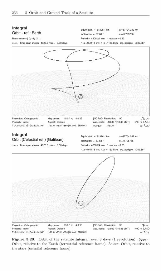
236 5 Orbit and Ground Track of a Satellite
IntegralOrbit - ref.: EarthRecurrence = [ 0; +1; 3] 1
>>>> Time span shown: 4320.0 min = 3.00 days
Equiv. altit. = 81326.1 km
e = 0.795766
a =87704.242 km
Inclination = 67.68 °
Period = 4308.24 min * rev/day = 0.33
h_a =151118 km; h_p =11534 km; arg. perigee: +302.88 °
[NORAD] Revolution: 90
Asc. node: -33.09 ° [10:48 LMT]
Apogee: -49.70 °
Projection: Orthographic
Property: none
T.:Azimuthal Graticule: 30°
Map centre: 15.0 ° N; 4.0 °E
Aspect: Oblique
[ -90.0 / +75.0 / +86.0 ] Gr.Mod.: GRIM5-C1
IntegralOrbit (Celestial ref.) [Galilean]>>>> Time span shown: 4320.0 min = 3.00 days
Equiv. altit. = 81326.1 km
e = 0.795766
a =87704.242 km
Inclination = 67.68 °
Period = 4308.24 min * rev/day = 0.33
h_a =151118 km; h_p =11534 km; arg. perigee: +302.88 °
[NORAD] Revolution: 90
Asc. node: -33.09 ° [10:48 LMT]
Projection: Orthographic
Property: none
T.:Azimuthal Graticule: 30°
Map centre: 15.0 ° N; 4.0 °E
Aspect: Oblique
[ -90.0 / +75.0 / +86.0 ] Gr.Mod.: GRIM5-C1
Figure 5.20. Orbit of the satellite Integral, over 3 days (1 revolution). Upper :Orbit, relative to the Earth (terrestrial reference frame). Lower : Orbit, relative tothe stars (celestial reference frame)

5.4 Classifying Satellites by Mission 237
IntegralElliptical orbit - Ground trackRecurrence = [ 0; +1; 3] 1
>>>> Time span shown: 4320.0 min = 3.00 days
Equiv. altit. = 81326.1 km
e = 0.795766
a =87704.242 km
Inclination = 67.68 °
Period = 4308.24 min * rev/day = 0.33
h_a =151118 km; h_p =11534 km; arg. perigee: +302.88 °
[NORAD] Revolution: 90
Asc. node: -33.09 ° [10:48 LMT]
Apogee: -49.70 °
Projection: Sanson-Flamsteed
Property: Equal area
T.:Pseudocylindr. Gratic.:10°
Map centre: 90.0 ° N; 0.0 °
Aspect: Polar
[ +90.0 / +90.0 / -90.0 ] Gr.Mod.: GRIM5-C1
FASTOrbit - ref.: EarthRecurrence = [11;+11; 71] 792
>>>> Time span shown: 4320.0 min = 3.00 days
Equiv. altit. = 2054.5 km
e = 0.202505
a = 8432.587 km
Inclination = 82.97 °
Period = 128.56 min * rev/day =11.20
h_a = 3762 km; h_p = 347 km; arg. perigee: +95.00 °
[NORAD] Revolution: 33065
Asc. node: 139.56 ° [07:54 LMT]
Apogee: -85.19 °
Projection: Orthographic
Property: none
T.:Azimuthal Graticule: 10°
Map centre: 28.0 ° N; 84.0 ° W
Aspect: Oblique
[ -90.0 / +62.0 / +174.0 ] Gr.Mod.: EGM96
Figure 5.21. Upper : Ground track of the satellite Integral, over 3 days (1 revolu-tion, recurrence cycle). Lower : Orbit of the satellite FAST, relative to the Earth

238 5 Orbit and Ground Track of a Satellite
ExosatEllipt. orbit - Gr. track>>>> Time span shown: 5760.0 min = 4.00 days
Equiv. altit. = 96109 km
e = 0.934449
a = 102487.1 km
Inclination = 72.50 °
Period = 5442.93 min * rev/day = 0.26
h_a =191878 km; h_p = 340 km; arg. perigee: +270.00 °
Longitude / Initialisation:
Asc. node: 90.00 °
Apogee: -135.42 °
Projection: Orthographic
Property: none
T.:Azimuthal Graticule: 10°
Map centre (r.): 52.0 ° N; 12.0 °E
Aspect: Oblique
[ -90.0 / +38.0 / +78.0 ] Gr.Mod.: GEM-T2
PolarEllipt. orbit - Gr. track>>>> Time span shown: 6.80 days
Equiv. altit. = 49802.9 km
e = 0.701000
a =56181.000 km
Inclination = 84.20 °
Period = 2208.88 min * rev/day = 0.65
h_a = 89186 km; h_p =10420 km; arg. perigee: +216.20 °
Longitude / Initialisation:
Asc. node: 20.00 °
Apogee: 27.60 °
Projection: Lorgna
Property: Equal area
T.:Azimuthal Graticule: 10°
Map centre (r.): 90.0 ° N; 10.0 °E
Aspect: Direct
[ -90.0 / +0.0 / +80.0 ] Gr.Mod.: GEM-T2
Figure 5.22. Ground tracks of HEO satellite orbits. Upper : Exosat over 4 days(1 revolution). Lower : Polar over 7 days (4 revolutions)

5.4 Classifying Satellites by Mission 239
Microwave. The US satellite COBE (Cosmic Background Explorer),launched in 1989 on a Sun-synchronous orbit at h = 880 km, i = 99.0,explored the millimetre radiation in space in order to study temperature fluc-tuations in the diffuse cosmological background via extremely precise mea-surements. (The temperature varies from 2.722 49 K to 2.722 51 K dependingon the observed region.) This informs us about fluctuations in the matter den-sity of the early universe. Its successor MAP (Microwave Anisotropy Probe,MIDEX-2), with angular resolution 0.2 as compared with 7 for COBE,is placed91 in L2LO orbit. The European satellite Planck92 (formerly CO-BRAS/SAMBA) launched slightly later, should further improve these results.It will also be placed at the point L2.
For the study of galactic molecular clouds, SWAS (Submillimeter WaveAstronomy Satellite, SMEX-3) was launched in 1998, and now follows a lowprograde orbit, with h = 640 km, i = 69.9.
Radio. The first satellites to study radio sources were RAE-A and -B (RadioAstronomy Explorer, Explorer-38 and -49), launched in 1968 and 1973 on ahighly inclined circular orbit with h = 5850 km and i = 120.9. The Japanesesatellite Haruka (Muses-B, ‘haruka’ means ‘remote’), launched in 1997, is onan HEO orbit, with hp = 569 km, ha = 21 415 km, i = 31.4. The Russianproject with European participation KRT-25 (a 25 m radio telescope) willbe placed in an orbit which, over seven years, will become more and moreeccentric: hp ≈ 5000 km, ha from 20 000 to 150 000 km, i = 63
Solar Astrophysics
Solar radiation is studied across the whole range of wavelengths. The Sun hasbeen the subject of investigation since the very beginning of the Space Age,from 1962 to 1976, with LEO satellites at altitudes between 500 and 600 km,such as the eight observatories OSO-1 to -8 (Orbiting Solar Observatory),i = 33 and three Explorers, IQSY (International Quiet Sun Year, Explorer-
91 Launched on 30 June 2001, the MAP probe made four revolutions around theEarth on ever more eccentric orbits, reaching the vicinity of the Moon a monthlater. Using a lunar swing-by, it took another two months to arrive at the pointL2 of the Sun–Earth system on 1 October 2001 and go into the halo orbit. MAPwas re-christened Wilkinson MAP (or WMAP) in February 2003, in honour ofDavid T. Wilkinson of Princeton University, a world-famous cosmologist andMAP team member who died in September 2002 at the age of 67.
92 Max Planck (1858–1947) was a German physicist. He studied blackbody ra-diation and found an expression for the blackbody spectrum as a function oftemperature and frequency. This problem had stumped many physicists beforehim. Planck solved it in 1900 by introducing the idea of the energy quantum.The theory of these quanta then became the basis for much of modern physics.
240 5 Orbit and Ground Track of a Satellite
30), Solrad-9 and -10 (Solar Radiation,93 Explorer-37 and -44), i ≈ 55, orwith slightly inclined HEO orbits, such as the EPE programme (EnergeticParticles Explorer), with EPE-A, -B, -C and -D (Explorer-12, -14, -15, -26).The German satellites Helios-1 and -2 are in heliocentric orbit (perihelion0.309 a.u., aphelion 0.985 a.u., i = 0, ecliptic plane, T = 190 day).
Launched in 1980, the US satellite SMM (Solar Maximum Mission) wasthe first satellite to be repaired in flight by the Shuttle STS-13 (STS-41-C),in 1984. It operated until 1989 on the orbit h = 405 km, i = 26.5.
Recent LEO satellites are in near-polar orbits. Some are Sun-synchronouslike the US satellites TRACE (Transition Region and Coronal Explorer,SMEX-4), with altitude h = 620 km, ACRIMSAT (Active Cavity Radiome-ter Irradiance Monitor Satellite), h = 700 km (launched in 1998 and 1999,respectively), or the French project Picard (see note on Picard), h = 700 km.Others are prograde, such as the Russian–Ukrainian satellites Koronas-I andKoronas-F (AUDS-SM-KI and -KF), h = 520 km, i = 82.5 (launched in1994 and 2001).94 The US satellite SORCE (Solar Radiation and ClimateExperiment) was launched in 2003 on the orbit h = 641 km, i = 40.0. Thesatellite Solar-B, currently in the planning stages for a Sun-synchronous or-bit, should take over from the Japanese Solar-A (or Yohkoh, ‘Sun’), whichwas launched in 1991 with hp = 526 km, ha = 795 km, i = 31.3.
Two large projects have inspired a collaboration between ESA and NASAin this area: Ulysses and SOHO. The Ulysses probe, launched on 6 October1990 from STS-41, set off first in the direction of Jupiter, to use it for agravity-assist maneuver (see Chap. 11) that would take it out of the plane ofthe ecliptic. On 1 November 1994 it overflew the south pole of the Sun and on1 October 1995, the north pole. The satellite SOHO (Solar and HeliosphericObservatory), launched on 2 December 1995, went to Lagrange point L1 toacquire a halo orbit. It subsequently discovered a great many comets.
Two projects should use the stable Lagrange points. The Japanese satel-lite L5-Mission will observe the Sun in order to provide a regular space‘weather’ forecast, and ensure better protection for space activities. The twoUS satellites STEREO (Solar-Terrestrial Relation Observatory) are plannedfor the Lagrange points, with STEREO-Ahead at L4, and STEREO-Behindat L5, thus providing a 3D observation of the Sun.93 It later transpired that the first Solrad missions, from Solrad-1 to -7B, between
1960 and 1965, were primarily spy satellites (ELINT). To give the Solrad pro-gramme a more scientific countenance, it was also referred to as GREB (GalacticRadiation Experimental Background) or GRAB (Galactic Radiation And Back-ground).
94 The letters I and F are the initials of IZMIRAN and FIRAS, the names of theinstitutes which designed the project.
5.4 Classifying Satellites by Mission 241
Stellar Seismology and the Search for Exoplanets
Three satellites, each carrying a small telescope, have been designed to studythe seismology of stars. They follow three very different orbits. The Cana-dian satellite MOST (Microvariability and Oscillations of Stars, jokingly nick-named the Humble Space Telescope by its developers), launched on 30 June2003, follows a Sun-synchronous orbit at h = 625 km, i = 98.7. The Danishsatellite MONS (Measuring Oscillations in Nearby Stars) is on a Molniya or-bit. The French satellite Corot (Convection, rotation et transits planetaires)is looking for planets in orbit around stars other than the Sun by detectingthe transit (when the planet passes in front of its star and thereby diminishesits luminosity), as well as studying stellar seismology. It has a circular, strictlypolar orbit with h = 827 km. These three satellites are a preparatory stage forthe European project Eddington,95 which will study the internal structure ofstars and seek to detect extra-solar planets. This satellite will be in an L2LOorbit. In November 2003, ESA postponed the mission indefinitely. Anotherproject, a forerunner of Eddington that has since been abandoned, wouldhave sent the satellite STARS to the Lagrange point L5 of the Earth–Moonsystem.
The European mission Darwin,96 will be devoted to astrobiology, but itis a long-term project. (One also uses the term ‘exobiology’ to remove allpossible confusion with ‘astrology’.) The Darwin ‘flotilla’97 will also be in
95 Arthur Stanley Eddington (1882–1944) was a British astronomer and physicist.He did much to promote the theory of relativity (see the note on Einstein),through the publication of his book Space, Time and Gravitation (1920), whichis still being reprinted. He also laid the foundations for a new discipline, stellardynamics, with The Internal Constitution of the Stars (1926), in which he showsthat a star is subject to two opposing effects: it tends to contract under the effectof gravity, whilst the release of energy tends to push it apart.
96 Charles Darwin (1809–1882) was an English naturalist. From 1831 to 1836, hetook part in an expedition to South America (and in particular, to the Galapa-gos islands) and Oceanica, aboard the HMS Beagle. As a geologist and botanist,he elaborated his theory of evolution on the basis of notes taken and collec-tions brought back from this expedition. He concluded that the variability of thespecies is due to the effects of their environment and to sudden variations. Thesevariations are only favoured by natural selection if they give the individual or-ganism an advantage in its struggle for survival (subsistence and reproduction).His famous book The Origin of Species was published in 1859. Darwin’s theory,supported and developed by a great many intellectuals, was attacked withoutscientific argument by the conservative-minded and religious classes. Here wasanother problem of divine order!
97 The Darwin flotilla comprises six satellites in formation. They lie strictly in thesame plane and each is equipped with a telescope in such a way as to form aninfrared interferometer. One master satellite, a short distance from the others,oversees the satellite positions and provides the link with the Earth. The aim is
242 5 Orbit and Ground Track of a Satellite
an L2LO orbit. The US project Kepler will follow a heliocentric orbit witha = 1.013 19 a.u., e = 0.03188, and T = 372.5 day.
Space Exploration
Probes sent out to observe other planets in the Solar System or their moonswill be studied in Chaps. 10 and 11, along with satellites in orbit aroundthese celestial bodies.
We restrict ourselves here to probes involved in the study of comets. Hal-ley’s comet,98 the most famous of all comets, was approached by six probesin March 1986: ISEE-3 renamed ICE for the mission, Vega-1 and -2 (So-viet probes, ‘Ve’ for ‘Venera’, ‘Ga’ for ‘Galleia’, ‘Venus’ and ‘Halley’ in Rus-sian), Giotto (a European probe, which flew by the cometary nucleus at only600 km), Sakigake and Suisei (Japanese probes, ‘scout’ and ‘comet’, respec-tively, in Japanese).
The CONTOUR probe (Comet Nucleus Tour) was launched on 3 July2002 and failed shortly afterwards. It was to investigate short period cometssuch as P/Encke, whose orbit never extends beyond that of Jupiter.
The Rosetta mission99 is one of ESA’s cornerstone missions. The probe,launched on 2 March 2004, should follow a complex path100 in order to ac-quire an orbit around comet101 67P/Churyumov-Gerasimenko in May 2114.In November 2114, the Philae module should land on the cometary nucleusand ride with it to its perihelion.
NASA’s Stardust and Genesis missions involve in situ exploration withsample-return.102
to detect planets orbiting other stars and to spy out possible signatures of lifebeyond our own Solar System.
98 Edmond Halley (1656–1742) was a British astronomer. In 1682, he observed avery bright comet near its perihelion. He calculated the orbital elements andpredicted that the comet would return in 1758. Once the period of 76 years hadbeen established, it was realised that this comet had been known since ancienttimes. The first pictorial representation was due to the Italian painter Giotto in1304. In 1716, Halley published a method using the transit of Venus, predictedfor 1761, to measure the distance from the Earth to the Sun.
99 The Rosetta stone carries a bilingual inscription in three scripts, which allowedthe French linguist Champollion to decipher the hieroglyphs of Ancient Egyptin 1822. The name Rosetta comes from ‘Rachid’, the Arabic name for the villagein the Nile delta where the stone was found. ESA chose this appellation for itscornerstone project because it expects the results to throw light upon some ofthe mysteries of the formation of the Solar System.
100 EMEEGA: Earth (March 2005) Mars (March 2007) Earth (November 2007)Earth (November 2009) Gravity Assist.
101 For the initially planned launch in January 2003, Rosetta was to meet up withcomet 46P/Wirtanen ten years on.
102 Stardust, launched on 7 February 1999, collected interstellar dust in 2002 andparticles from comet Wild-2 on 2 January 2004. The capsule should be returned
5.4 Classifying Satellites by Mission 243
5.4.8 Technological Satellites
This is the category of satellites whose mission it is to assist in various kindsof technological development. The very first satellites fit well in this class.Technological satellites are used to test instruments, orbital maneuvers, com-munication techniques, and reentry vehicles (RV technology). They are alsoused to test the design of electric or ion propulsion motors.
The satellite DODGE (Department Of Defense Gravity Experiment), h =33 400 km, i = 12, was sent into space in 1967 to further the development ofgeostationary satellites, although the first had already been launched someyears previously. A camera aboard this satellite took the very first colourpictures of the Earth’s disk.
The military satellite ARGOS (Advanced Research Global ObservationSatellite or P91-1) was launched into a Sun-synchronous LEO orbit in 1999to test electric propulsion systems and detect X rays.
To study the effect of radiation on various types of equipment, severalsmall technological satellites have been placed in highly elliptical orbits.These are in fact the geostationary transfer orbits (GTO) of the main satel-lites with which they were launched (see the lower part of Fig. 5.10). SuchGTO orbits expose the satellites to an extremely testing environment, sincethey cross the Van Allen radiation belts on each revolution. With this mis-sion, we find the British microsatellites STRV (Space Technology ResearchVehicle), hp = 300 km, ha = 36 000 km, i = 7, STRV-1A and -1B launchedin 1994 as passengers with Intelsat-702, and STRV-1C and -1D in 2000, pas-sengers with PAS-1R (PanAmSat-1R). Likewise for Teamsat, launched withthe geostationary satellite Maqsat. The Japanese satellite MDS-1 (MissionDemonstration Satellite) will go into a more highly inclined GTO orbit, withi = 28.5.
This category also covers calibration satellites, such as Radcal, h ≈800 km, i = 89.5, for radar calibrations, Reflektor, launched with Meteor-3M-1, for laser calibrations, and the twelve nanosatellites (a few kg) launchedby STS-60 and -63, ODERACS-A to -F, and ODERACS-2A to -2F (OrbitalDebris Radar Calibration Sphere), to calibrate spacecraft debris.
One type of experiment, called a tether experiment, involves connectingthe satellite to a secondary body once it is already in orbit, using cables ofdifferent lengths. These cables may or may not be conducting. The first testswere carried out on the manned flights Gemini-11 and -12 (with a cable of
to the Utah desert on 15 January 2006. Stardust’s heliocentric orbit involves onetrip beyond the orbit of Mars.Genesis, launched on 8 August 2001, reached LOI (Lissajous Orbit Insertion) on16 November 2001. After two years at Lagrange point L1 (halo orbit), it collectedparticles from the solar wind and returned the sample. The capsule was to havebeen ejected and recovered by helicopter in the Utah desert, on 8 September2004. However, the parachutes failed to deploy, resulting in a hard-landing, andthe samples are considered to be virtally unusable.
244 5 Orbit and Ground Track of a Satellite
30 m). Also worth mentioning, launched into LEO orbit between 1993 and1996, are the satellites SEDS-1 then -2 (Small Expendable Deployer System),with cables 20 km long, and TiPS (Tether Physics and Survivability), witha 4 km cable. The orbit of the TiPS central satellite had the characteristics:h = 1 022 km, i = 63.4, e = 0.000.
Among planned missions, we note the BOLAS experiment (Bistatic Ob-servations with Low Altitude Satellites), devoted to the study of the iono-sphere with a view to improving communications for GPS. It consists of twosatellites, BOLAS-1 and -2, connected by a non-conducting cable 100 m longand rotating about their centre of gravity. They will be launched at the sametime as Radarsat-2, on a Sun-synchronous orbit, and will then acquire anelliptical orbit with hp = 350 km, ha = 800 km, i = 102.81.
In the United States, the universities carry out missions with small tech-nological satellites, such as TERRIERS or SNOE (Student Nitric Oxide Ex-plorer). In Europe, this policy is mainly applied in the United Kingdom, withthe UoSAT (University of Surrey Satellites), and in Germany with the Tubsat(Technische Universitat Berlin Satellites). These satellites, which can gener-ally be subsumed under the heading of technological satellites, are almostalways placed in Sun-synchronous orbits as passengers.
In this category we may also include satellites with biology missions. Thesatellite Sputnik-2 carried a female dog aboard. Animals were sent in theRussian Bion satellites to study the effects of radiation. For example, in 1996,two monkeys flew in Bion-11, h = 300 km, i = 63. We may also mentionthe US LEO satellite OFO-1 (Orbital Frog Otolith), occupied by two toads.The aim was to study their inner ear, seat of the vestibular organ (balancesystem).
5.4.9 Satellites with Specific Military Missions
Many programmes have been developed by the military and civilian sectors,either jointly or in parallel, with similar areas of interest, such as remote-sensing, surveillance and communications. However, certain programmes arespecifically military, such as the detection of nuclear explosions. Here is abrief review.
Early Warning
These satellites are designed to detect enemy missiles as soon as possibleduring or after their launch. In the United States, the first programme wasMIDAS (Missile Defense Alarm System), with near-polar LEO satellites, h ≈3000 km, from MIDAS-3 in 1962 to MIDAS-12 in 1966. Satellites in thefollowing programme, IMEWS (Integrated Missile Early Warning Satellites),extended by DSP (Defense Support Program), have been geostationary, i ≈0, from IMEWS-2 in 1971 to DSP-F-21 (USA-159) in 2001, and DSP-F-22

5.4 Classifying Satellites by Mission 245
(USA-176) in 2004. The NMD project (National Missile Defense), currentlyunder discussion, is based on the SBIRS satellites (Space-Based IR System).As soon as a missile is fired, it is detected by SBIRS-High (a system of 4 GEOsatellites and 2 HEO satellites). The missile is then tracked by SBIRS-Low(a constellation of 24 satellites in 6 orbital planes).
The Soviet programme SPRN was equivalent to IMEWS, with a fleet ofGEO satellites. Satellites in the Oko series (‘eye’) are in Molniya orbit, fromKosmos-520 in 1972 to Kosmos-2368 in 1999.
Nuclear Surveillance
In order to keep an eye on nuclear testing, the various space powers havelaunched satellites that can detect explosion by their gamma-ray emissions.The US satellites Vela had novel circular orbits, at very high altitudes h ≈110 000 km, and with inclinations varying between 34 and 61. They werelaunched in pairs, diametrically opposed with respect to the centre of theEarth, from Vela-1 and -2 in 1963 to Vela-11 and -12 in 1970, and remainedoperational until 1984. (‘Vela’ means ‘lookout’ in Spanish. These satelliteswere also called Watchdogs or Vela Hotel.) They fullfilled a scientific missionthat had not been planned at all at the outset: between 1969 and 1979,the satellites Vela-9 and -10 (OPS/6909 and OPS/6911), Vela-11 and -12(OPS/7033 and OPS/7044) mapped gamma-ray sources in space. They werethe first to observe what have since become known as gamma-ray bursts(GRB).
Destruction of Satellites, Star Wars
It is of little interest in this context to dwell upon satellite destruction pro-grammes like ASAT (Air-Launched Anti-Satellite Missile), FOBS (FractionalOrbital Bombardment System), or what is popularly referred to as ‘star wars’,i.e., the US programme SDI (Space Defense Initiative).
Intelligence
Satellite interception of all kinds of electronic signal is considered to be ofgreat importance by the military. This is SIGINT (signal intelligence) orELINT (electronic intelligence). Military photographic surveillance is IMINT(image intelligence). The US–British (and Commonwealth) project Echelonis planning a constellation of 120 satellites.
The US SIGINT missions began with the GREB (or GRAB) series andFerret (beginning in 1962 with Ferret-2), on LEO orbits. Subsequently, thewhole range of different orbits was used. Each programme lasted for roughlya decade. We note the following programmes, from the second generation(the 1970s) to the fifth (the 2000s):
246 5 Orbit and Ground Track of a Satellite
• LEO: SSF (Subsatellite Ferrets), NOSS (Navy Ocean Surveillance Satel-lite, also called White Cloud) and NOSS-Sub-sats (satellites in formation),SB-WASS (Space-Based Wide Area Surveillance System), SB-WASS NextGeneration (with planned orbits inclined at 155).
• HEO: Jumpseat, Trumpet,103 Prowler.• GEO: Canyon, Rhyolite/Aquacade, Chalet/Vortex, Magnum/Orion, Mer-
cury,104 Mentor, Intruder.
There have been similar Soviet then Russian programmes, beginning in 1970with Kosmos-389. The Tselina programme, in LEO orbit, is the equivalentof NOSS, with i = 82.6 for the Tselina-D series and i = 71.0 for the mostrecent Tselina-2 series.
5.4.10 Satellites with Human Occupation
We give here a few dates marking out the history of manned spaceflight,i.e., satellites in orbit with humans aboard: Vostok-1 (‘Orient’ in Russian),launched on 12 April 1961, for the first man in orbit (one revolution); Apollo-11, launched on 16 July 1969, for the first man on the Moon.
The idea of an orbital space station was first put into practice with theSoviet Salyut (‘salvation’) from 1971 to 1986, followed by Mir (‘mir’ meansboth ‘world’ and ‘peace’ in Russian) from 1986 to 2000, on a near-circularorbit, h ∼ 300 km, i = 51.6. The United States used Skylab, in 1973, onan equivalent orbit, h ∼ 400 km, i = 50.0. They then began to develop theISS (International Space Station), from 1998, in collaboration with Russiaand other nations. The orbit is circular, with h between 355 and 400 km,i = 51.6.
The space shuttle idea is based on the possibility of a reusable space-craft, a satellite becoming a plane in the landing stage. The five AmericanSpace Shuttles are Columbia (1981–2003), Challenger (1983–1986), Discov-ery (since 1984), Atlantis (since 1985), Endeavour (since 1992). Their flightsare numbered with the prefix STS (Space Transportation System). At theend of 2003, there had been 113 shuttle flights: 111 successes, 2 failures, withChallenger STS-33 (STS-51-L) and Columbia STS-107.
The shuttle has two configurations: a payload of 24.4 tonnes for a loworbit, h = 204 km, i = 28.5, and a payload of 12.5 tonnes for a higherorbit, h = 407 km, i = 51.6. It is the latter configuration that is used
103 The three satellites in the series Trumpet-1 (USA-103), Trumpet-2 (USA-112)and Trumpet-3 (USA-136) were launched between 1994 and 1997. They followMolniya orbits with apogee over Russia. Their antennas have diameters of severaltens of metres, and between 100 and 150 m apparently for Trumpet-3. Data iscollected by the SDS satellites, also in Molniya orbit.
104 Mercury-1 (USA-105 or Jeroboam) and Mercury-2 (USA-118) were launched in1994 and 1996. This programme is sometimes called Mercury ELINT to distin-guish it from the Mercury programme of manned flights.
5.5 Appendix: Velocity of Satellite and Ground Track in Circular Orbit 247
for rendezvous with ISS. For maintenance of Hubble, the shuttle goes into ahigher orbit. A great many satellites have been placed in orbit by the shuttle.Once in orbit, the satellite leaves the cargo bay of the shuttle and moves toits destination under its own power (a nearby orbit, either geostationary orheliocentric).
5.4.11 Non-Scientific Satellites
The Celestis satellites are placed under the ‘others’ heading of the miscella-neous category in the otherwise rather detailed sample listed in the Celestrakdirectory. Furthermore, they are the only representatives of this category.Other US organisations classify them as burial satellites.105 Without wishingto carry out unnecessary advertising for the Celestis company, we merely notethat the orbit of Celestis-1 has the high inclination of 151 (because launchedwith Minisat-01). Celestis-2 has an inclination of 108 (because launched withGFO-1) and Celestis-3 is Sun-synchronous (launched with ACRIMSAT andKompsat). They have altitude h ∼ 700 km. Celestis-4 burnt up in space fol-lowing launch failure (grouped with OrbView-4 and QuikTOMS). Note thatthese satellites have been renamed Earthview-01, -02, -03 and -04, whichmight lead to some surprises in a remote-sensing bibliography.
5.5 Appendix: Velocity of Satellite and Ground Trackin Circular Orbit
Accurate calculation of the satellite velocity can be achieved using the equa-tions of motion discussed in Chap. 3. Here we shall calculate the velocityof the satellite and its ground track to very high accuracy, considering thecase of circular and Keplerian motion. This discussion could well have beenincluded in Chap. 2. However, we prefer to present it here, now that we havedefined the angular velocity of the Earth’s rotation and the different types ofsatellite, especially geosynchronous satellites.
5.5.1 Definitions of the Different Velocities
The velocity of the satellite S and that of its ground track S0, in , can beexpressed in a simple manner in terms of the mean motion n :
105 Taking a closer look, one may read in the informative note of the Celestis com-pany: ‘Celestis offers to launch a symbolic portion of the cremated remains ofthe individuals into space.’ Business is clearly booming: several satellites havebeen placed in orbit since 1997, not to mention a lunar impact with Lunar-01(in fact, a capsule carried by Lunar Prospector) in 1998, following the same idea.There is a project to send such spacecraft into deep space and out of the SolarSystem.

248 5 Orbit and Ground Track of a Satellite
Table 5.2. Velocity of satellite and ground track, and relative velocity of the groundtrack for various satellites, in circular (Keplerian) orbit. For each satellite, we givethe altitude h (in km) and the length of the semi-major axis a, or distance from thecentre of the Earth (in km), the daily frequency ν (in revs per day), the Keplerianperiod T0 (in hours and minutes), the speeds V , V0, wE (for the three values of theangle i, 0, 90, 180), defined in the present section (in kms−1). Also given is thecorresponding type of satellite T : GL (ground level), E (espionage, surveillance), SS(space shuttle, manned flights and Earth observation), O (Earth observation fromLEO orbit), G (geodesy), I (communications with ICO-type orbit, between LEOand MEO), P (positioning by GPS from MEO orbit), S (geostationary, GEO), V(Vela-type), M (Moon)
h a ν T0 V V0 wE wE wE T[km] [km] [rev/day] [d h m] 0 90 180
0 6378 17.04 1h24 7.91 7.91 7.44 7.92 8.37 GL100 6478 16.65 1h26 7.84 7.72 7.26 7.74 8.19 E200 6578 16.27 1h28 7.78 7.55 7.08 7.56 8.01 E300 6678 15.91 1h31 7.73 7.38 6.91 7.39 7.84 SS400 6778 15.56 1h33 7.67 7.22 6.75 7.23 7.68 SS500 6878 15.22 1h35 7.61 7.06 6.60 7.07 7.52 O600 6978 14.89 1h37 7.56 6.91 6.44 6.92 7.37 O700 7078 14.58 1h39 7.50 6.76 6.30 6.78 7.23 O800 7178 14.28 1h41 7.45 6.62 6.16 6.64 7.09 O900 7278 13.98 1h43 7.40 6.49 6.02 6.50 6.95 O
1000 7378 13.70 1h45 7.35 6.35 5.89 6.37 6.82 O1100 7478 13.42 1h47 7.30 6.23 5.76 6.24 6.69 O1200 7578 13.16 1h49 7.25 6.10 5.64 6.12 6.57 O1300 7678 12.90 1h52 7.21 5.99 5.52 6.00 6.45 O1400 7778 12.66 1h54 7.16 5.87 5.41 5.89 6.33 O1500 7878 12.42 1h56 7.11 5.76 5.29 5.78 6.22 O1600 7978 12.18 1h58 7.07 5.65 5.19 5.67 6.11
2000 8378 11.32 2h07 6.90 5.25 4.79 5.27 5.713000 9378 9.56 2h31 6.52 4.43 3.97 4.46 4.904000 10378 8.21 2h55 6.20 3.81 3.34 3.84 4.275000 11378 7.15 3h21 5.92 3.32 2.85 3.35 3.78 G6000 12378 6.30 3h48 5.67 2.92 2.46 2.96 3.39 G
10390 16768 4.00 6h00 4.88 1.85 1.39 1.91 I20183 26561 2.01 11h58 3.87 0.93 0.47 1.04 P35786 42164 1.00 23h56 3.07 0.47 0.00 S
110000 116378 0.22 4d13h45 1.85 0.10 −0.36 0.47 V
376805 383183 0.04 27d07h43 1.02 0.02 M
5.5 Appendix: Velocity of Satellite and Ground Track in Circular Orbit 249
V =d(OS)
dt, V = an =
õ
a, (5.33)
V 0 =d(OS0)
dt, V0 = Rn =
R
aV =
R
a
õ
a. (5.34)
In the terrestrial frame T, consider a point on the surface of the Earth,e.g., S0, and the right-handed triple of unit vectors associated with sphericalcoordinates (er, eλ, eφ). In a plane tangent to the Earth (local horizontalplane), the plane (eλ, eφ), the vector eλ lies along a line of latitude and thevector eφ lies along a meridian. In this frame, the velocity of the groundtrack, which we shall denote by w, is equal to
w = V 0 − R cosφ ΩTeλ .
If eu is the unit vector along V 0, we obtain the expression for w, whichcan be called the relative velocity of the ground track, or the velocity of theground track relative to the ground:
w = R(neu − ΩT cosφeλ
). (5.35)
5.5.2 Velocity at the Equator
To compare values obtained for various satellites, we consider the relativevelocity w and the ascending (or descending) node, i.e., at the equator, whereit will be written wE :
wE
R= neu − ΩTeλ .
It can be written in terms of the inclination i of the satellite aswE
R=(n cos i − ΩT
)eλ + n sin i eφ . (5.36)
Let wE be the magnitude of wE taken in the direction of the velocity. Weobtain the results for three values of the inclination, namely, i = 0, i = 90
and i = 180, respectively:
wE
R= n − ΩT ,
wE
R=√
n2 + Ω2T ,
wE
R= n + ΩT . (5.37)
Table 5.2 shows for various satellites the velocity of the satellite and itsground track, V and V0, in , and the relative velocities of the ground trackwE, in T for these three values of i. Satellites are represented for a wholerange of altitudes between 0 and 1600 km, in steps of 100 km, and then fora few altitudes characteristic of various types of mission.
250 5 Orbit and Ground Track of a Satellite
The maximal velocity of the ground track relative to the ground is8.4 kms−1, obtained for a retrograde satellite moving at ground level. Morerealistically, the velocity of the ground track at the equator for an operationalSun-synchronous satellite is 6.6 km s−1. For a geosynchronous satellite withi = 0, hence geostationary, we may check that wE = wE(i = 0) = 0.00.
The last satellite in the table is not as artificial as it may look. It is in facta simplified model of the Moon, in circular, Keplerian orbit at a distance of380 000 km, with period about 27 day. Note that, in , the sidereal period isequal to 27.32 day, whilst in T, the synodic period106 which takes the Earth’smotion into account, is equal to 29.53 day, a lunar month.107 The synodicperiod T ′ (in days) is calculated using the relation (2.23), with T = 27.32and T1 = Nsid.
5.6 Appendix: Satellite Visibility Time
The span of time over which a satellite S is visible from a given point P onthe Earth is called the visibility time of S from P . This idea arises mainly inthe study of satellite constellations.
5.6.1 Satellite in Circular Orbit
Consider an arbitrary point P on the (spherical) surface of the Earth anda satellite S whose orbital plane passes through P at a given time. This isshown schematically in Fig. 5.23 (upper). The satellite S can be seen from Pas long as it remains above the local horizon for P , represented by the straightline S1PS2, i.e., on the circular arc S1AS2. The angle α = (OP , OS1) canbe found immediately (reduced distance η):
cosα =R
R + h=
R
a=
1η
. (5.38)
The period of the satellite is taken equal to the Keplerian period T0. Thevisibility time ∆tv is therefore
106 The noun , ‘synod’, is composed from , ‘with, together’ and
, ‘way, journey’. In Ancient Greek, it already had the two meanings of‘meeting’ and ‘conjunction of heavenly bodies’, both of which illustrate the ideaof arriving at the same time.
107 In English it is no accident that the word ‘month’ should be so similar to the word‘Moon’. This similarity can be found in German and other related languages. TheIndo-European root ∗men, ∗mes refers to the Moon, to lunation (= month), andto measurement (of time). Many languages in this family have held on to thisproximity of meaning, although this has not happened in Greek or Latin. Thesetwo languages referred to the Moon as ‘the shining one’ ( and luna,æ). See also the note on Chandrasekhar.

5.6 Appendix: Satellite Visibility Time 251
∆tv =α
πT0 . (5.39)
Expressing α and T0 as functions of the semi-major axis a (here the radius)of the orbit, we obtain
∆tv = 2
√a3
µarccos
R
a. (5.40)
Using the altitude h and the value of the period T0(h=0) defined by (2.17),we have (for time in minutes and angles in radians)
∆tv (min) = 84.5(
1 +h
R
)3/2 1π
arccosR
R + h. (5.41)
One may also consider the question by fixing a minimal zenithal angle of sightζ, with ζ = (PA, PS′
1). The visibility time then corresponds to the timetaken by the satellite to travel along the arc S′
1AS′2. In this case, the angle
α = (OP , OS′1) depends on η and ζ. Simple trigonometric considerations
(projecting S′1 on PA) show that this angle is the solution of the equation
cosα − 1tan ζ
sin α =1η
.
Hence,
α = 2 arctan√
1 + Z2 − H2 − Z
1 + H. (5.42)
with H = 1/η , Z = 1/ tan ζ ,
and we obtain the visibility time from (5.39).When the satellite does not pass through the vertical at the relevant point,
the visibility time is obviously shorter.
Example 5.6. Calculate the visibility time for LEO and MEO satellites.
For a (SPOT-type) LEO satellite with h = 800 km, we find η = 1.125 and T0 =101 min. Using (5.38), we obtain α = 27 and hence, by (5.39),
∆tv = (27/180) × 101 = 15 min .
If the visibility condition consists in requiring that the satellite should be at least15 above the horizon, i.e., ζ = 75, the calculation with (5.42) gives α = 16 andwe deduce that ∆tv = 9 min. These visibility times are maximal values, assumingthat the satellite passes through the local vertical.For a (NAVSTAR/GPS-type) MEO satellite with h = 20 200 km, we find η = 4.167and T0 = 718 min. It follows that α = 76 and hence,
∆tv = (76/180) × 718 = 304 min ≈ 5 hr .
With ζ = 60 (visibility if the satellite is more than 30 above the horizon), we
have α = 48 and ∆tv = 192 min ≈ 3 hr.
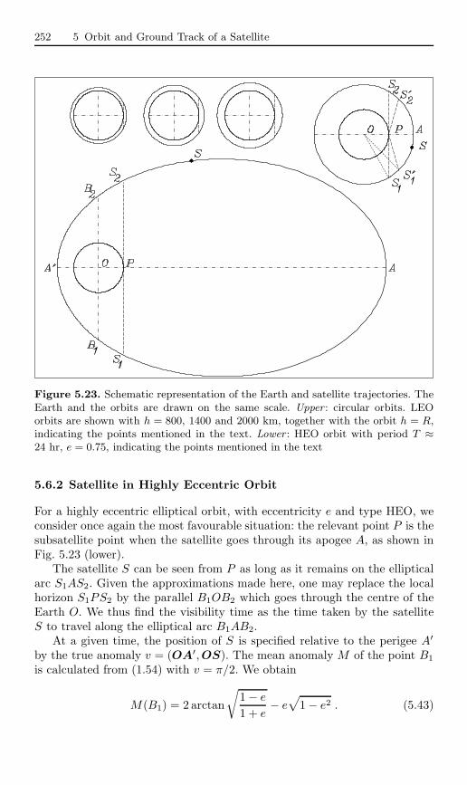
252 5 Orbit and Ground Track of a Satellite
Figure 5.23. Schematic representation of the Earth and satellite trajectories. TheEarth and the orbits are drawn on the same scale. Upper : circular orbits. LEOorbits are shown with h = 800, 1400 and 2000 km, together with the orbit h = R,indicating the points mentioned in the text. Lower : HEO orbit with period T ≈24 hr, e = 0.75, indicating the points mentioned in the text
5.6.2 Satellite in Highly Eccentric Orbit
For a highly eccentric elliptical orbit, with eccentricity e and type HEO, weconsider once again the most favourable situation: the relevant point P is thesubsatellite point when the satellite goes through its apogee A, as shown inFig. 5.23 (lower).
The satellite S can be seen from P as long as it remains on the ellipticalarc S1AS2. Given the approximations made here, one may replace the localhorizon S1PS2 by the parallel B1OB2 which goes through the centre of theEarth O. We thus find the visibility time as the time taken by the satelliteS to travel along the elliptical arc B1AB2.
At a given time, the position of S is specified relative to the perigee A′
by the true anomaly v = (OA′, OS). The mean anomaly M of the point B1
is calculated from (1.54) with v = π/2. We obtain
M(B1) = 2 arctan
√1 − e
1 + e− e√
1 − e2 . (5.43)
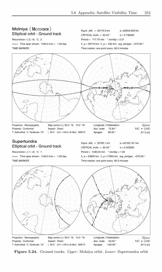
5.6 Appendix: Satellite Visibility Time 253
MolniyaElliptical orbit - Ground trackRecurrence = [ 2; +0; 1] 2
>>>> Time span shown: 1440.0 min = 1.00 day
TIME MARKER
Equiv. altit. = 20175.5 km
e = 0.736000
a =26553.629 km
CRITICAL Inclin. = 63.42 °
Period = 717.75 min * rev/day = 2.01
h_a = 39719 km; h_p = 632 km; arg. perigee: +270.00 °
Time marker: one point every 60.0 minutes
Longitude / Initialisation:
Asc. node: 72.94 °
Apogee: 80.00 °
Projection: Stereographic
Property: Conformal
T.:Azimuthal Graticule: 10°
Map centre (r.): 90.0 ° N; 10.0 ° W
Aspect: Direct
[ -90.0 / +0.0 / +100.0 ] Gr.Mod.: GEM-T2
SupertundraElliptical orbit - Ground trackRecurrence = [ 1; +0; 1] 1
>>>> Time span shown: 1440.0 min = 1.00 day
TIME MARKER
Equiv. altit. = 35785.1 km
e = 0.423000
a =42163.191 km
CRITICAL Inclin. = 63.43 °
Period = 1436.03 min * rev/day = 1.00
h_a = 53620 km; h_p =17950 km; arg. perigee: +270.00 °
Time marker: one point every 60.0 minutes
Longitude / Initialisation:
Asc. node: -53.02 °
Apogee: -100.00 °
Projection: Stereographic
Property: Conformal
T.:Azimuthal Graticule: 10°
Map centre (r.): 90.0 ° N; 10.0 ° W
Aspect: Direct
[ -90.0 / +0.0 / +100.0 ] Gr.Mod.: GEM-T2
Figure 5.24. Ground tracks. Upper : Molniya orbit. Lower : Supertundra orbit

254 5 Orbit and Ground Track of a Satellite
We deduce the visibility time as a function of the period:
∆tv =[1 − M(B1)
π
]T0 . (5.44)
Example 5.7. Calculate the visibility time for HEO satellites.
For a (Molniya-type) HEO satellite, we have e = 0.736 and T0 = 718 min. From(5.43) and (5.44), we obtain
M(B1) = 0.744 − 0.498 = 0.245 rad = 14 , 1 − 14/180 = 0.92 .
During one revolution, the satellite thus spends 92% of its time in going from B1 toB2 via A (and 8% in going from B2 to B1 via A′), which corresponds to ∆tv = 11 hrfor a period of 12 hr.108 This result appears clearly in Fig. 5.24 (upper), where thetime interval between two consecutive points marked on the ground track of theorbit is one hour. If we impose a minimal zenithal angle of sight ζ ∼ 70 and if P isnot exactly at the subsatellite point of A, we obtain a visibility span of about 8 hr.For a (Supertundra-type) HEO satellite, we have e = 0.423 and T0 = 1436 min. Weobtain
M(B1) = 0.751 rad = 43 , 1 − 43/180 = 0.76 ,
which represents a visibility time of 18 hr, illustrated in Fig. 5.24 (lower). Imposing
the above restrictions, a time of more than 12 hr is nevertheless obtained.
5.7 Appendix: NORAD Orbital Elements
The organisation known as NORAD (North American Aerospace DefenceCommand), founded in 1962, provides an inventory of all orbiting objects(satellites, whether active or otherwise, rocket debris, etc.). The position ofthe object on its orbit and the position of the orbit relative to the ECIGalilean frame109 are defined by the orbital elements. The calculated posi-tions are adjusted by radar measurements.
This data, referred to as the NORAD Two-Line Element Set Format, isupdated twice a day and can be accessed by Internet. Data for each satelliteconsists of three lines in the following format:
AAAAAAAAAAAAAAAAAAAAAAAA
1 NNNNNU NNNNNAAA NNNNN.NNNNNNNN +.NNNNNNNN +NNNNN-N +NNNNN-N N NNNNN
2 NNNNN NNN.NNNN NNN.NNNN NNNNNNN NNN.NNNN NNN.NNNN NN.NNNNNNNNNNNNNN
108 We observe that, although the name Molniya, lightning, suggests speed, it iswhen the satellite is at its slowest that it is actually used.
109 Earth-Centered Inertial (ECI) coordinate system: the z axis runs along theEarth’s rotational axis pointing North, the x axis points in the direction of thevernal equinox, and the y axis completes the direct orthogonal system.
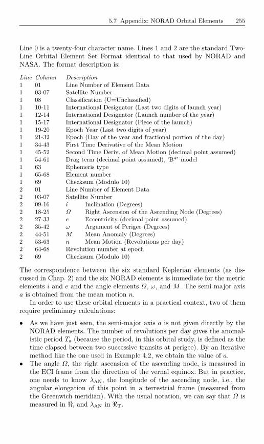
5.7 Appendix: NORAD Orbital Elements 255
Line 0 is a twenty-four character name. Lines 1 and 2 are the standard Two-Line Orbital Element Set Format identical to that used by NORAD andNASA. The format description is:
Line Column Description1 01 Line Number of Element Data1 03-07 Satellite Number1 08 Classification (U=Unclassified)1 10-11 International Designator (Last two digits of launch year)1 12-14 International Designator (Launch number of the year)1 15-17 International Designator (Piece of the launch)1 19-20 Epoch Year (Last two digits of year)1 21-32 Epoch (Day of the year and fractional portion of the day)1 34-43 First Time Derivative of the Mean Motion1 45-52 Second Time Deriv. of Mean Motion (decimal point assumed)1 54-61 Drag term (decimal point assumed), ‘B*’ model1 63 Ephemeris type1 65-68 Element number1 69 Checksum (Modulo 10)2 01 Line Number of Element Data2 03-07 Satellite Number2 09-16 i Inclination (Degrees)2 18-25 Ω Right Ascension of the Ascending Node (Degrees)2 27-33 e Eccentricity (decimal point assumed)2 35-42 ω Argument of Perigee (Degrees)2 44-51 M Mean Anomaly (Degrees)2 53-63 n Mean Motion (Revolutions per day)2 64-68 Revolution number at epoch2 69 Checksum (Modulo 10)
The correspondence between the six standard Keplerian elements (as dis-cussed in Chap. 2) and the six NORAD elements is immediate for the metricelements i and e and the angle elements Ω, ω, and M . The semi-major axisa is obtained from the mean motion n.
In order to use these orbital elements in a practical context, two of themrequire preliminary calculations:
• As we have just seen, the semi-major axis a is not given directly by theNORAD elements. The number of revolutions per day gives the anomal-istic period Ta (because the period, in this orbital study, is defined as thetime elapsed between two successive transits at perigee). By an iterativemethod like the one used in Example 4.2, we obtain the value of a.
• The angle Ω, the right ascension of the ascending node, is measured inthe ECI frame from the direction of the vernal equinox. But in practice,one needs to know λAN, the longitude of the ascending node, i.e., theangular elongation of this point in a terrestrial frame (measured fromthe Greenwich meridian). With the usual notation, we can say that Ω ismeasured in , and λAN in T.
256 5 Orbit and Ground Track of a Satellite
We first calculate the angle ΩG00 between the Greenwich meridian and thevernal equinox at 0 h UTC, on the relevant day. This angle corresponds to themean sidereal time GMST (Greenwich Mean Sidereal Time), at 0 h, writtenqG00 and measured in seconds. It is obtained from the relation
qG00 = 24110.54841 + 8640184.812866Tu + 9.3 × 10⁻²T 2u − 6.2 × 10⁻⁶T 3
u ,(5.45)
where Tu = du/36525 and du is the number of days elapsed since 1 January2000 at 12 h, which corresponds to the Julian date JD 2 451 545.0.
With the equivalence between days and round trips (1 day – 360), weobtain ΩG00 in degrees from qG00 in seconds:
ΩG00 =qG00
240. (5.46)
We then calculate ΩGt, the angle between the Greenwich meridian and thevernal equinox at the relevant UT time:
ΩGt = ΩG00 + ΩT∆t , (5.47)
where ΩT is the angular speed of rotation of the Earth, in degrees/day, givenby (4.22), and ∆t is the fraction of the day elapsed at the relevant UT timesince 0 hr UT.
The positions of the ascending node and the Greenwich meridian, Ω andΩGt, respectively, are measured from the same origin at the same time. Wethus obtain the longitude λAN of the ascending node in a terrestrial frame:
λAN = Ω − ΩGt . (5.48)
The longitude and the UT time then give the LMT crossing time at theascending node.
Example 5.8. Calculate the orbital elements of the ICESat satellite from theNORAD elements.
During the first few months of its mission, the satellite ICESat followed a so-calledcalibration orbit. Its ground track had to repeat every 8 days (we return to thenotion of recurrence in Chap. 7). The calibration orbit overflew the White Sandsground station calibration site every 8 days. Once the satellite and its instrumentshad been commissioned, burns were performed to attain ICESat’s 183-day repeatground track, mission orbit. The NORAD elements for the given day during thiscalibration phase were as follows:
ICESAT
1 27642U 03002A 03175.25018279 .00000722 00000-0 75456-4 0 1631
2 27642 94.0031 263.4514 0002250 85.5696 274.5785 14.90462832 24163
We obtain the date from
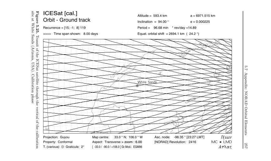
5.7
Appen
dix
:N
OR
AD
Orb
italE
lemen
ts257
ICESat [cal.]Orbit - Ground trackRecurrence = [15; -1; 8] 119
>>>> Time span shown: 8.00 days
Altitude = 593.4 km
e = 0.000225
a = 6971.515 km
Inclination = 94.00 °
Period = 96.68 min * rev/day =14.89
Equat. orbital shift = 2694.1 km ( 24.2 °)
Asc. node: -98.35 ° [23:27 LMT]
[NORAD] Revolution: 2416
Projection: Guyou
Property: Conformal
T.:(various) Graticule: 2°
Map centre: 33.0 ° N; 106.0 ° W
Aspect: Transverse > zoom : 6.00
[ -33.0 / -90.0 / +106.0 ] Gr.Mod.: EGM96
Fig
ure
5.2
5.Tra
nsit
ofth
eIC
ESat
satellite
thro
ugh
the
vertica
lofth
eca
libra
tion
siteat
White
Sands
(Arizo
na,U
SA
).C
alib
ratio
nphase
258 5 Orbit and Ground Track of a Satellite
03175.25018279: year = 03, day = 175, hour = 0.25018279/24 ,
which gives 24 June 2003, at 06:00:15.79 UTC. Just for information, this was revo-lution number 2416, counting from the satellite’s first transit at the ascending node.The following elements are obtained immediately:
n = 14.904 628 32 rev/day , e = 0.000 225 0 , i = 94.003 1 ,
Ω = 263.451 4 , ω = 85.569 6 , M = 274.578 5 .
With the mean anomaly M , we can calculate the eccentric and true anomalies, veryclose to M since the eccentricity is extremely small: E = 274.566 and v = 274.553.With n, we find the anomalistic period Ta (min) = 1440/n, or Ta = 96.614 28 min.To begin with, we set T0 = Ta, and with this Keplerian period, we obtain thevalue of the semi-major axis of the Keplerian orbit: a0 = 6974.6 km. We calculatethe secular variation related to the mean motion, ∆n/n = −0.6695 × 10⁻³, thenrecalculate a. After several iterations, this yields a = 6971.515 km, that is, analtitude of h = a − R = 593 km. With the values of a and i, we can calculate theprecession rates and periods. This yields:
nodal precession Ω = +0.5079/day ,
apsidal precession ω = −3.5508/day ,
anomalistic period Ta = 96.6143 min ,
draconitic period Td = 96.6782 min.
To calculate the longitude of the ascending node, we determine the Julian dateof the relevant time, JD 2 452 814.750, which gives JD-JD2000 = 1 269.750 andhence du = 1269.5. Using (5.45), we obtain qG00 = 65 217.588 (mod 86 400), orΩG00 = 271.740 . Given the fraction of the day elapsed, we obtain from (5.47),ΩGt = 1.806 whence, by (5.48),
λAN = 263.451 − 1.806 = 261.646 .
For a transit at the ascending node at longitude 261.646 (i.e., 98.354W), the time
06:00 UT corresponds to 23:27 LMT. These elements suffice to represent the ground
track of the ICESat satellite over 8 days. During this time, the satellite should pass
through the vertical at the calibration site in White Sands (Arizona). Figure 5.25
shows that this constraint was respected.
5.8 Appendix: Cartographic Projections
A cartographic projection is a transformation mapping a point of the sphere(or an ellipsoid), specified by its spherical coordinates λ, φ (longitude, lati-tude), in a bijective manner onto its coordinates x, y on the map:
cartographic projection f = f1, f2
x = f1(λ, φ) ,y = f2(λ, φ) .
5.8 Appendix: Cartographic Projections 259
There exist infinitely many such projections.The main problem to be solved by a cartographic projection can be put
succinctly as follows: the sphere is not developable. This means that the sur-face of a sphere cannot be mapped onto a plane without distorting or tearingit.110 Theoretical study of this question was carried out contemporaneouslyby Lambert111 (1772), Euler (1777) and Lagrange (1779). It was definitivelysolved by Gauss (1822), who studied the conditions under which an arbitrarysurface could be mapped onto another arbitrary surface.
A cartographic projection can have (exclusively) one or other of the fol-lowing two properties:
• angles are conserved, and the projection is said to be conformal,• areas are conserved, and the projection is said to be equal area or equiv-
alent.
It may be that it has neither of these properties,112 but it can never haveboth. In fact, the map can conserve the angles or the area of a figure, butit can never conserve the perimeter. No map can conserve distances in alldirections. In other words, no projection can have constant scale over thewhole field of projection.
In a conformal projection, the parallels and the meridians on the mapintersect at right-angles, since the same is true on the sphere, where they formtwo sets of orthogonal curves. In an equal area projection, a country twice asbig as another is represented on the map by an area twice as big. When thewhole Earth is represented, it can be considered as spherical since projectingthe terrestrial sphere or ellipsoid on a plane leads to quite imperceptibledifferences in the resulting maps, whatever projection may be used. The sameis not true for accurate regional maps, however.
Projections can be classified by type or by aspect. The type tells us howthe sphere appears when projected onto the map, i.e., cylindrical, conical,
110 Unlike the sphere, a cylinder is developable. If the body of a big cat could beassimilated to a cylinder, one could understand how the tiger might change intoa bedside rug without deformation.
111 Jean Henri Lambert (1728–1777) was a Swiss and German astronomer, math-ematician and physicist, with French ancestry. In astronomy, he calculated thetrajectories of comets and understood that the Milky Way was just a modestgalaxy in the Universe. In physics, he discovered the fundamental law of pho-tometry. In his many mathematical works, among which he demonstrated theirrationality of π (1766), he assigned great importance to problems of perspec-tive and cartographic projections. He defined a great many projections, several ofwhich bear his name today. The best known is the conformal conical projection,used in France for the map of France since 1922 and the cadastral survey since1938.
112 The older literature is full of different adjectives describing these properties: au-togonal and orthomorphic for conformal; authalic, homolographic for equivalent;aphylactic, in the absence of these properties. Such terms have now gone intodisuse.

260 5 Orbit and Ground Track of a Satellite
EnvisatOrbit - Ground trackRecurrence = [14;+11; 35] 501
>>>> Time span shown: 5760.0 min = 4.00 days
Altitude = 781.4 km a = 7159.497 km
Inclination / SUN-SYNCHRON.= 98.55 °
Period = 100.60 min * rev/day =14.31
Equat. orbital shift = 2799.7 km ( 25.1 °)
Asc. node: 0.13 ° [22:00 LMT]
App. inclin. = 102.46 °
Projection: Snyder-Satel.Track/55°
Property: none
T.:Cylindrical Graticule: 10°
Map centre: 0.0 ° ; 0.0 °
Aspect: Direct
[ +0.0 / +0.0 / +0.0 ] Gr.Mod.: GEM-T2
Jason-1Orbit - Ground trackRecurrence = [13; -3; 10] 127
>>>> Time span shown: 10.00 days
Altitude = 1336.3 km a = 7714.434 km
Inclination = 66.04 °
Period = 112.43 min * rev/day =12.81
Equat. orbital shift = 3155.5 km ( 28.3 °)
Asc. node: 99.92 °
App. inclin. = 70.29 °
Projection: Snyder-Satel.Track/35°
Property: none
T.:Cylindrical Graticule: 10°
Map centre: 0.0 ° ; 0.0 °
Aspect: Direct
[ +0.0 / +0.0 / +0.0 ] Gr.Mod.: GEM-T2
Figure 5.26. Ground tracks of two Sun-synchronous and prograde satellites. Sny-der projection, with different standard parallels. Upper : 55. Lower : 35
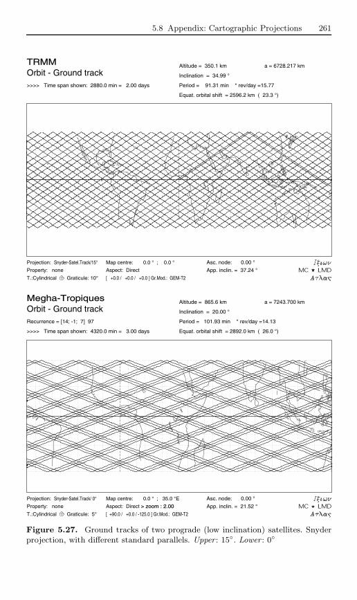
5.8 Appendix: Cartographic Projections 261
TRMMOrbit - Ground track>>>> Time span shown: 2880.0 min = 2.00 days
Altitude = 350.1 km a = 6728.217 km
Inclination = 34.99 °
Period = 91.31 min * rev/day =15.77
Equat. orbital shift = 2596.2 km ( 23.3 °)
Asc. node: 0.00 °
App. inclin. = 37.24 °
Projection: Snyder-Satel.Track/15°
Property: none
T.:Cylindrical Graticule: 10°
Map centre: 0.0 ° ; 0.0 °
Aspect: Direct
[ +0.0 / +0.0 / +0.0 ] Gr.Mod.: GEM-T2
Megha-TropiquesOrbit - Ground trackRecurrence = [14; -1; 7] 97
>>>> Time span shown: 4320.0 min = 3.00 days
Altitude = 865.6 km a = 7243.700 km
Inclination = 20.00 °
Period = 101.93 min * rev/day =14.13
Equat. orbital shift = 2892.0 km ( 26.0 °)
Asc. node: 0.00 °
App. inclin. = 21.52 °
Projection: Snyder-Satel.Track/ 0°
Property: none
T.:Cylindrical Graticule: 5°
Map centre: 0.0 ° ; 35.0 °E
Aspect: Direct > zoom : 2.00
[ +90.0 / +0.0 / -125.0 ] Gr.Mod.: GEM-T2
Figure 5.27. Ground tracks of two prograde (low inclination) satellites. Snyderprojection, with different standard parallels. Upper : 15. Lower : 0
262 5 Orbit and Ground Track of a Satellite
azimuthal, and so on. We use the word ‘appears’ because a cartographicprojection is not usually (and the exceptions are very rare) a projection inthe sense of an intersection between a straight line and a plane. For example,the Mercator projection is said to be cylindrical, but it is not the ‘projection’of this sphere from its centre onto a cylinder that is tangent to it at theequator (as one often reads).
The aspect of a projection can be direct (or normal), transverse, oroblique. For example, for a stereographic projection (of azimuthal type) withdirect aspect (also called polar in this case), the point of contact of the planeof projection with the sphere occurs at the pole, whilst it occurs on the equa-tor for a transverse projection (also called equatorial in this case). For anarbitrary point of contact, the projection is said to be oblique.
The computer software Atlas, which we have devised, is coupled with theorbitography part of our program Ixion. Any satellite ground track can thusbe mapped out with the chosen projection. In each representation, everyeffort is made to apply the most suitable cartographic projection. On all themaps presented here, plotted using Atlas, we indicate the main features ofthe projection: name, properties, type and aspect. Also given in the key arethe coordinates (longitude and latitude) of the centre of the map, togetherwith the three Euler angles which define the rotation of the globe for thisprojection from the standard initial position.
The projections used in the present book can be grouped as follows:
• Conformal Projections. The angle between the ground track (of thesatellite or its swath) and the given meridian is conserved. The mainprojections here are:– the Mercator projection,– the stereographic projection,– the projections due to Guyou and Adams, based on elliptic integrals
of the first kind.• Equal Area Projections. These projections are used when it is im-
portant to respect surface areas. The main projections used in this bookare:– the Behrmann projection (dilated Lambert equal area cylindrical pro-
jection) and the Lorgna projection,– the Mollweide and Sanson projections,– the Goode homolosine projection (in interrupted form),– the Hammer–Aitoff projection.
• Perspective Projections. Although they have no special properties,these projections are rather visual, representing the planet as if it wereseen from space, viewed from various distances. The main projectionsused are:– the perspective view projection, where the viewing point is at a finite
distance (expressed as a number of planetary radii),– the orthographic projection, where the viewing point is at infinity,
5.8 Appendix: Cartographic Projections 263
– the Armadillo projection, due to Raisz, which represents the sphere ina rather picturesque manner projected on a torus.
• Specific Projections. In 1977, the American cartographer John P. Sny-der invented a specific projection to represent satellite ground tracks forthe satellite ERTS-1 (Landsat-1) and the following satellites in the Land-sat programme. This projection, Satellite Tracking, keeps the meridiansregularly spaced and modifies the spacing of the parallels in such a waythat the satellite ground track is a straight line. We have adapted thisto any type of satellite. It is presented in the two parts of Fig. 5.26 andFig. 5.27, with four different dilatations of the latitudes.
• Archaic Projection. The so-called plate-carree projection is very fre-quently used (if not exclusively) in books and documents concerned withsatellite ground tracks. It represents longitudes and latitudes linearlyalong the abscissa and ordinate, respectively. This projection is some-what simple-minded (x = λ, y = φ), even primitive (it was fashionable. . . in the Middle Ages). It has no particular properties (it is neither con-formal, nor equivalent) and its only mathematical value is its simplicity.This is no longer an argument with the advent of computer programming.It has not been used here, except for the first three maps in the book, atthe beginning of the chapter. (We did not wish to upset habits too earlyon.)


SpringerParisBerlinHeidelbergNew YorkHong KongLondresMilanTokyo
Michel Capderou
SatellitesOrbits and Missions
Translated from French by Stephen Lyle
Michel CapderouL.M.D.École Polytechnique91128 [email protected]
TranslatorStephen LyleAndebu09240 [email protected]
Ouvrage publié avec le concours du Ministère français chargé de la culture- Centre national du livrePublication supported by the French Ministry of Culture - National Book Centre
ISBN : 2-287-21317-1
© Springer-Verlag France 2005Imprimé en FranceSpringer-Verlag France est membre du groupe Springer Science + Business Media
© Springer-Verlag France 2003, for the original publication in French
Apart from any fair dealing for the purposes of the research or private study, or criticism or review, as permitted underthe Copyright, Designs and Patents Act 1998, this publication may only be reproduced, stored or transmitted, in anyform or by any means, with the prior permission in writing of the publishers, or in the case of reprographic reproduc-tion in accordance with the terms of licenses issued by the copyright. Enquiry concerning reproduction outside thoseterms should be sent to the publishers.The use of registered names, trademarks, etc, in this publication does not imply, even in the absence of a specific state-ment, that such names are exempt from the relevant laws and regulations and therefore free for general use.
SPIN: 10994245
Cover design : Nadia OUDDANE
This eBook does not include ancillary media that was packaged with the printed version of the book.

Foreword
In all, the European Space Agency (ESA) has developed 60 spacecrafts overthe last few decades. Some of these, such as the ERS satellites and Envisat,are dedicated to monitoring the Earth and providing vital data on the healthstatus of our planet. Other spacecraft have helped to improve the accuracyof weather forecasting. Galileo, the joint ESA/EU satellite navigation pro-gramme, demonstrates the political dimension of space as service-providerfor the benefit of European citizens. While these missions involve utilitarianspace activities, others are devoted to either exploring the solar system, in-cluding the Sun, or achieving a better understanding of the Universe and thecosmic beginnings.
The orbits of these satellites cover a wide range (Sun-synchronous, geosta-tionary, highly eccentric, at Lagrange points, etc.) so that a complete novicemay be astonished when tackling the space technology field. The main creditof Michel Capderou’s book is to take the reader (whether it be a student,an engineer or a research scientist) progressively from the basic Kepler lawsto the most complex equations of space mechanics. His educational concernhas led him to propose many examples and graphical illustrations from ESA,but also from the American, Russian, Indian, Japanese or even Chinese spaceagencies. These programmes provide scientific insights and moreover appearto fascinate the general public, in particular the younger generation. Thosewishing to understand the orbital mechanisms behind these programmes willfind the explanations they seek in this book.
Paris, France
Jean-Jacques Dordain, ESA Director General
December 2004
Foreword to the French Edition
For more than forty years now, space science has revolutionised a wholerange of fields including telecommunications, data transmission, meteorology,geodesy, precise positioning on the Earth’s surface, and Earth observation forboth civilian and military purposes. Within science itself, it has added a newdimension to astronomy and astrophysics, to the study of the Solar Systemand planets, and to our understanding of the mechanisms underlying thebehaviour of the various subsystems making up the Earth environment, i.e.,the atmosphere, the oceans, the biosphere, the continental surfaces, and thecryosphere. Space is now opening up to biology and medecine, and is used asa laboratory for fundamental physics.
These advances are of course due to the invention and development ofever more sophisticated methods of communication and observation, mak-ing either active or passive use of the whole range of the electromagneticspectrum, from the shortest wavelengths associated with X and gamma rays,to microwaves and centimetre waves. However, they also owe much to thecapability developed by research teams and engineers in the world’s spaceagencies to position satellites and space probes with greater and greater ac-curacy on orbits selected to fulfill the commercial, operational or scientificaims of today’s missions. Indeed, an Earth-observation system, no matterhow advanced it may be, will never yield the results required of it unless it isplaced on an appropriate orbit and with suitable orientation, so that it candeliver the predefined spatial and temporal resolutions. Likewise, a communi-cations or positioning system, based for example on a satellite constellation,will not achieve its objectives unless the orbits are correctly chosen to guaran-tee full temporal coverage. Finally, space probes and large space observatoriesin different ranges of the electromagnetic spectrum will only lead us to a bet-ter understanding of the origin and evolution of our Universe and the SolarSystem if they are adequately placed to observe the relevant objects.
With this in mind, Michel Capderou’s book makes an essential contribu-tion to our understanding of the problems raised by the precise determinationof satellite and space probe orbits. His approach, based on physics and me-chanics, reminds us that the underlying principles of celestial mechanics basedon the theory of gravitation were brought to light by the great names of sci-ence, from Tycho Brahe and Copernicus to Newton, from Kepler and Galileo
VIII Foreword
to Laplace, from Lagrange to Poincare and Einstein. But this does not meanthat orbital calculations are any the simpler, and they appear in their fullcomplexity as soon as the relevant problem involves the mutual attractions ofseveral interacting bodies, or requires some consideration of perturbations tothe system, due for example to spatial and temporal anomalies in the Earth’sgravitational field. But it is to Michel Capderou’s credit that he manages toinitiate us in the mathematical and physical techniques of orbit calculationswhilst nevertheless bringing out the full scope of the problem. Basing hispresentation on concrete examples which refer to real missions under devel-opment or already launched, we are brought to a better understanding of therelative advantages of the different types of satellite orbit and positioningcurrently used. The completeness of this treatise guarantees its success as atextbook, just as the accompanying software, developed and perfected by theauthor himself, will help the reader to build up the kind of three-dimensionalvision that is a prerequisite to space observation, so that he or she may thenbe able to design the orbit and mission appropriate to the problem at hand.Michel Capderou’s book is an essential element for any student, engineer orresearch scientist involved in space science.
Paris, France Gerard Megie, President CNRSJuly 2002 Professor, Pierre & Marie Curie University
Preface
Space mechanics is one thing, but space missions are many and varied. Indeed,they are involved in the detection of forest fires and cyclones, television relay,positioning on the globe to within a metre, measurement of sea level, and thesearch for water on Mars, to mention but a few. Since 1957, several thousandsatellites have been launched and 1 200 satellite names appear in the indexto this book.
It is in this spirit of duality that the book was written: on the one side,the ‘eternal’ laws of mechanics, and on the other, the rationale behind eachtype of orbit, given the temporal constraints laid down by the nature of itsmission. The text is divided into four parts.
In the first part (Chaps. 1–3), which deals with the motion of the satellite,it is difficult to be innovative with the fundamental laws of dynamics and thetheory of perturbations. We have introduced a great many figures in the hopeof making this part appear less theoretical.
In the second part (Chaps. 4–7), which is devoted to the orbit and itsground track, we begin to present new tools that we have developed to providea clearer presentation of these key notions, such as the use of the constantof Sun-synchronicity kh, or the frequency κ and the index Φ for the studyof recurrence. The theory is abundantly illustrated by examples relating to awide range of satellite trajectories, be they circular or elliptical, low or high,or characterised in some other way.
In the next part (Chaps. 8–9), which treats the questions of spatial andtemporal sampling, we begin to examine the instruments carried aboard insuch a way as to describe what they will see from this vantage point. We studythe geometry of the satellite–target and satellite–target–Sun configurations.This part is particularly concerned with Earth-observation satellites.
The results of these three parts are all taken up again in the last part ofthe book, comprising Chaps. 10 and 11, where we consider a satellite aroundMars or some other celestial body.
Ixion, our orbitography and sampling software, provides the backbone ofthis book. It originated in preparations for the ScaRaB project, a radiometerdesigned by the LMD. Two models were carried aboard the Russian satellitesMeteor-3-07 in 1994 and Resurs-O1-4 in 1998. The software was originally
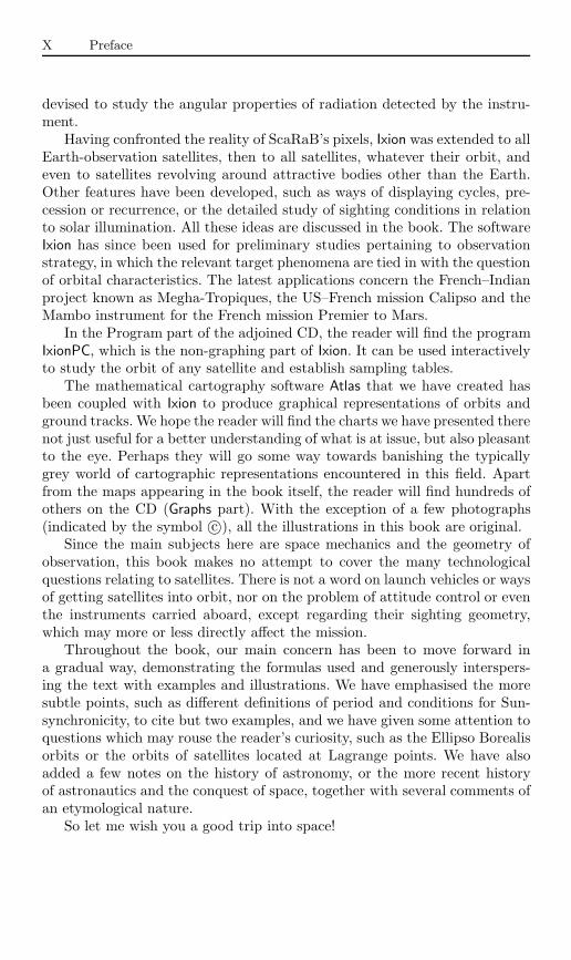
X Preface
devised to study the angular properties of radiation detected by the instru-ment.
Having confronted the reality of ScaRaB’s pixels, Ixion was extended to allEarth-observation satellites, then to all satellites, whatever their orbit, andeven to satellites revolving around attractive bodies other than the Earth.Other features have been developed, such as ways of displaying cycles, pre-cession or recurrence, or the detailed study of sighting conditions in relationto solar illumination. All these ideas are discussed in the book. The softwareIxion has since been used for preliminary studies pertaining to observationstrategy, in which the relevant target phenomena are tied in with the questionof orbital characteristics. The latest applications concern the French–Indianproject known as Megha-Tropiques, the US–French mission Calipso and theMambo instrument for the French mission Premier to Mars.
In the Program part of the adjoined CD, the reader will find the programIxionPC, which is the non-graphing part of Ixion. It can be used interactivelyto study the orbit of any satellite and establish sampling tables.
The mathematical cartography software Atlas that we have created hasbeen coupled with Ixion to produce graphical representations of orbits andground tracks. We hope the reader will find the charts we have presented therenot just useful for a better understanding of what is at issue, but also pleasantto the eye. Perhaps they will go some way towards banishing the typicallygrey world of cartographic representations encountered in this field. Apartfrom the maps appearing in the book itself, the reader will find hundreds ofothers on the CD (Graphs part). With the exception of a few photographs(indicated by the symbol c©), all the illustrations in this book are original.
Since the main subjects here are space mechanics and the geometry ofobservation, this book makes no attempt to cover the many technologicalquestions relating to satellites. There is not a word on launch vehicles or waysof getting satellites into orbit, nor on the problem of attitude control or eventhe instruments carried aboard, except regarding their sighting geometry,which may more or less directly affect the mission.
Throughout the book, our main concern has been to move forward ina gradual way, demonstrating the formulas used and generously interspers-ing the text with examples and illustrations. We have emphasised the moresubtle points, such as different definitions of period and conditions for Sun-synchronicity, to cite but two examples, and we have given some attention toquestions which may rouse the reader’s curiosity, such as the Ellipso Borealisorbits or the orbits of satellites located at Lagrange points. We have alsoadded a few notes on the history of astronomy, or the more recent historyof astronautics and the conquest of space, together with several comments ofan etymological nature.
So let me wish you a good trip into space!
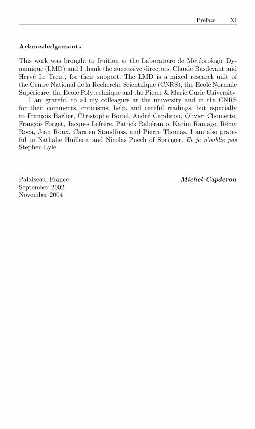
Preface XI
Acknowledgements
This work was brought to fruition at the Laboratoire de Meteorologie Dy-namique (LMD) and I thank the successive directors, Claude Basdevant andHerve Le Treut, for their support. The LMD is a mixed research unit ofthe Centre National de la Recherche Scientifique (CNRS), the Ecole NormaleSuperieure, the Ecole Polytechnique and the Pierre & Marie Curie University.
I am grateful to all my colleagues at the university and in the CNRSfor their comments, criticisms, help, and careful readings, but especiallyto Francois Barlier, Christophe Boitel, Andre Capderou, Olivier Chomette,Francois Forget, Jacques Lefrere, Patrick Raberanto, Karim Ramage, RemyRoca, Jean Roux, Carsten Standfuss, and Pierre Thomas. I am also grate-ful to Nathalie Huilleret and Nicolas Puech of Springer. Et je n’oublie pasStephen Lyle.
Palaiseau, France Michel CapderouSeptember 2002November 2004
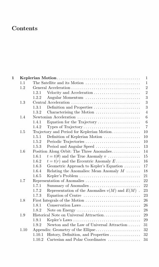
Contents
1 Keplerian Motion . . . . . . . . . . . . . . . . . . . . . . . . . . . . . . . . . . . . . . . . . 11.1 The Satellite and its Motion . . . . . . . . . . . . . . . . . . . . . . . . . . . 11.2 General Acceleration . . . . . . . . . . . . . . . . . . . . . . . . . . . . . . . . . . 2
1.2.1 Velocity and Acceleration . . . . . . . . . . . . . . . . . . . . . . . 21.2.2 Angular Momentum . . . . . . . . . . . . . . . . . . . . . . . . . . . 3
1.3 Central Acceleration . . . . . . . . . . . . . . . . . . . . . . . . . . . . . . . . . . 31.3.1 Definition and Properties . . . . . . . . . . . . . . . . . . . . . . . 31.3.2 Characterising the Motion . . . . . . . . . . . . . . . . . . . . . . 4
1.4 Newtonian Acceleration . . . . . . . . . . . . . . . . . . . . . . . . . . . . . . . 61.4.1 Equation for the Trajectory . . . . . . . . . . . . . . . . . . . . . 61.4.2 Types of Trajectory . . . . . . . . . . . . . . . . . . . . . . . . . . . . 7
1.5 Trajectory and Period for Keplerian Motion . . . . . . . . . . . . . . 101.5.1 Definition of Keplerian Motion . . . . . . . . . . . . . . . . . . 101.5.2 Periodic Trajectories . . . . . . . . . . . . . . . . . . . . . . . . . . . 101.5.3 Period and Angular Speed . . . . . . . . . . . . . . . . . . . . . . 13
1.6 Position Along Orbit: The Three Anomalies . . . . . . . . . . . . . . 141.6.1 t = t(θ) and the True Anomaly v . . . . . . . . . . . . . . . . 151.6.2 t = t(r) and the Eccentric Anomaly E . . . . . . . . . . . . 161.6.3 Geometric Approach to Kepler’s Equation . . . . . . . . 171.6.4 Relating the Anomalies: Mean Anomaly M . . . . . . . 181.6.5 Kepler’s Problem . . . . . . . . . . . . . . . . . . . . . . . . . . . . . . 21
1.7 Representation of Anomalies . . . . . . . . . . . . . . . . . . . . . . . . . . . 221.7.1 Summary of Anomalies . . . . . . . . . . . . . . . . . . . . . . . . . 221.7.2 Representation of the Anomalies v(M) and E(M) . 231.7.3 Equation of Centre . . . . . . . . . . . . . . . . . . . . . . . . . . . . 23
1.8 First Integrals of the Motion . . . . . . . . . . . . . . . . . . . . . . . . . . . 261.8.1 Conservation Laws . . . . . . . . . . . . . . . . . . . . . . . . . . . . . 261.8.2 Note on Energy . . . . . . . . . . . . . . . . . . . . . . . . . . . . . . . 28
1.9 Historical Note on Universal Attraction. . . . . . . . . . . . . . . . . . 291.9.1 Kepler’s Laws . . . . . . . . . . . . . . . . . . . . . . . . . . . . . . . . . 291.9.2 Newton and the Law of Universal Attraction . . . . . . 31
1.10 Appendix: Geometry of the Ellipse . . . . . . . . . . . . . . . . . . . . . . 321.10.1 History, Definition, and Properties . . . . . . . . . . . . . . . 321.10.2 Cartesian and Polar Coordinates . . . . . . . . . . . . . . . . 34
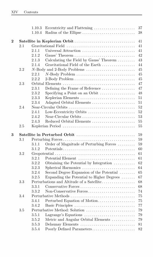
XIV Contents
1.10.3 Eccentricity and Flattening . . . . . . . . . . . . . . . . . . . . . 371.10.4 Radius of the Ellipse . . . . . . . . . . . . . . . . . . . . . . . . . . . 38
2 Satellite in Keplerian Orbit . . . . . . . . . . . . . . . . . . . . . . . . . . . . . . . 412.1 Gravitational Field . . . . . . . . . . . . . . . . . . . . . . . . . . . . . . . . . . . 41
2.1.1 Universal Attraction . . . . . . . . . . . . . . . . . . . . . . . . . . . 412.1.2 Gauss’ Theorem . . . . . . . . . . . . . . . . . . . . . . . . . . . . . . . 422.1.3 Calculating the Field by Gauss’ Theorem . . . . . . . . . 432.1.4 Gravitational Field of the Earth . . . . . . . . . . . . . . . . . 44
2.2 N -Body and 2-Body Problems . . . . . . . . . . . . . . . . . . . . . . . . . 452.2.1 N -Body Problem . . . . . . . . . . . . . . . . . . . . . . . . . . . . . . 452.2.2 2-Body Problem . . . . . . . . . . . . . . . . . . . . . . . . . . . . . . . 45
2.3 Orbital Elements . . . . . . . . . . . . . . . . . . . . . . . . . . . . . . . . . . . . . 472.3.1 Defining the Frame of Reference . . . . . . . . . . . . . . . . . 472.3.2 Specifying a Point on an Orbit . . . . . . . . . . . . . . . . . . 482.3.3 Keplerian Elements . . . . . . . . . . . . . . . . . . . . . . . . . . . . 512.3.4 Adapted Orbital Elements . . . . . . . . . . . . . . . . . . . . . . 51
2.4 Near-Circular Orbits . . . . . . . . . . . . . . . . . . . . . . . . . . . . . . . . . . 522.4.1 Low-Eccentricity Orbits . . . . . . . . . . . . . . . . . . . . . . . . 522.4.2 Near-Circular Orbits . . . . . . . . . . . . . . . . . . . . . . . . . . . 532.4.3 Reduced Orbital Elements . . . . . . . . . . . . . . . . . . . . . . 55
2.5 Keplerian Period . . . . . . . . . . . . . . . . . . . . . . . . . . . . . . . . . . . . . 55
3 Satellite in Perturbed Orbit . . . . . . . . . . . . . . . . . . . . . . . . . . . . . . 593.1 Perturbing Forces . . . . . . . . . . . . . . . . . . . . . . . . . . . . . . . . . . . . . 59
3.1.1 Order of Magnitude of Perturbing Forces . . . . . . . . . 593.1.2 Potentials . . . . . . . . . . . . . . . . . . . . . . . . . . . . . . . . . . . . . 60
3.2 Geopotential . . . . . . . . . . . . . . . . . . . . . . . . . . . . . . . . . . . . . . . . . 613.2.1 Potential Element . . . . . . . . . . . . . . . . . . . . . . . . . . . . . 613.2.2 Obtaining the Potential by Integration . . . . . . . . . . . 623.2.3 Spherical Harmonics . . . . . . . . . . . . . . . . . . . . . . . . . . . 643.2.4 Second Degree Expansion of the Potential . . . . . . . . 653.2.5 Expanding the Potential to Higher Degrees . . . . . . . 67
3.3 Perturbations and Altitude of a Satellite . . . . . . . . . . . . . . . . . 683.3.1 Conservative Forces . . . . . . . . . . . . . . . . . . . . . . . . . . . . 683.3.2 Non-Conservative Forces . . . . . . . . . . . . . . . . . . . . . . . . 74
3.4 Perturbative Methods . . . . . . . . . . . . . . . . . . . . . . . . . . . . . . . . . 753.4.1 Perturbed Equation of Motion . . . . . . . . . . . . . . . . . . . 753.4.2 Basic Principles . . . . . . . . . . . . . . . . . . . . . . . . . . . . . . . 77
3.5 Perturbative Method: Solution . . . . . . . . . . . . . . . . . . . . . . . . . 793.5.1 Lagrange’s Equations . . . . . . . . . . . . . . . . . . . . . . . . . . 793.5.2 Metric and Angular Orbital Elements . . . . . . . . . . . . 793.5.3 Delaunay Elements . . . . . . . . . . . . . . . . . . . . . . . . . . . . 813.5.4 Poorly Defined Parameters . . . . . . . . . . . . . . . . . . . . . . 82

Contents XV
3.5.5 Perturbative Accelerationsnot Derived from a Potential . . . . . . . . . . . . . . . . . . . . 83
3.6 Perturbative Method: Results for the Geopotential up to J2 833.6.1 Expression for Perturbative Potential up to J2 . . . . 833.6.2 Variation of the Orbital Elements . . . . . . . . . . . . . . . . 86
3.7 Perturbative Method: Results for General Case . . . . . . . . . . . 893.7.1 Geopotential up to Jn . . . . . . . . . . . . . . . . . . . . . . . . . . 893.7.2 Full Geopotential . . . . . . . . . . . . . . . . . . . . . . . . . . . . . . 943.7.3 Terrestrial and Non-Terrestrial Perturbations . . . . . . 95
3.8 Different Definitions of Period . . . . . . . . . . . . . . . . . . . . . . . . . . 963.9 Precessional Motion . . . . . . . . . . . . . . . . . . . . . . . . . . . . . . . . . . . 98
3.9.1 Precession of the Equinoxes . . . . . . . . . . . . . . . . . . . . . 983.9.2 Precession of the Line of Nodes of a Satellite . . . . . . 993.9.3 The Earth as a Satellite . . . . . . . . . . . . . . . . . . . . . . . . 100
3.10 Historical Note on Geodesy . . . . . . . . . . . . . . . . . . . . . . . . . . . . 1013.10.1 Calculating the J2 Term Using Geodesy . . . . . . . . . . 1013.10.2 Clairaut’s Formula . . . . . . . . . . . . . . . . . . . . . . . . . . . . . 1033.10.3 Terrestrial Ellipsoid . . . . . . . . . . . . . . . . . . . . . . . . . . . . 105
3.11 Geoid . . . . . . . . . . . . . . . . . . . . . . . . . . . . . . . . . . . . . . . . . . . . . . . 1073.11.1 Satellites and Geodesy . . . . . . . . . . . . . . . . . . . . . . . . . 1073.11.2 Development of Geopotential Models . . . . . . . . . . . . . 1093.11.3 Evaluation of the Geocentric Gravitational Constant112
3.12 Appendix: Astronomical Constants . . . . . . . . . . . . . . . . . . . . . 1123.13 Appendix: Gravitational Sphere of Influence . . . . . . . . . . . . . 114
3.13.1 Attraction of the Sun and Earth . . . . . . . . . . . . . . . . . 1143.13.2 Sphere of Influence . . . . . . . . . . . . . . . . . . . . . . . . . . . . . 116
3.14 Appendix: Lagrange Points . . . . . . . . . . . . . . . . . . . . . . . . . . . . 1173.14.1 Restricted Three-Body Problem . . . . . . . . . . . . . . . . . 1173.14.2 Simplified Study of Points L1 and L2 . . . . . . . . . . . . . 1183.14.3 The Five Lagrange Points . . . . . . . . . . . . . . . . . . . . . . 1203.14.4 Lagrange Points in Astronomy . . . . . . . . . . . . . . . . . . 1203.14.5 Artificial Satellites at Lagrange Points . . . . . . . . . . . . 122
3.15 Appendix: Summary of Legendre Functions . . . . . . . . . . . . . . 1243.16 Appendix: Spherical Trigonometry . . . . . . . . . . . . . . . . . . . . . . 125
3.16.1 Gauss’ Relations . . . . . . . . . . . . . . . . . . . . . . . . . . . . . . . 1253.16.2 Fifteen Relations for the Spherical Triangle . . . . . . . 125
4 Motion of Orbit, Earth and Sun . . . . . . . . . . . . . . . . . . . . . . . . . . 1294.1 Motion of the Orbit . . . . . . . . . . . . . . . . . . . . . . . . . . . . . . . . . . . 129
4.1.1 Secular Variations. Simplified Case . . . . . . . . . . . . . . . 1294.1.2 Secular Variations up to J4 . . . . . . . . . . . . . . . . . . . . . 1354.1.3 Applications: Period and Altitude . . . . . . . . . . . . . . . 1374.1.4 Strictly Polar Satellites . . . . . . . . . . . . . . . . . . . . . . . . . 141
4.2 Motion of the Earth . . . . . . . . . . . . . . . . . . . . . . . . . . . . . . . . . . 1424.2.1 Motion of the Earth about the Sun . . . . . . . . . . . . . . 143
XVI Contents
4.2.2 Motion of the Earth about the Polar Axis . . . . . . . . 1444.2.3 Motion of the Orbit and Earth . . . . . . . . . . . . . . . . . . 145
4.3 Apparent Motion of the Sun . . . . . . . . . . . . . . . . . . . . . . . . . . . 1464.3.1 Celestial Sphere and Coordinates . . . . . . . . . . . . . . . . 1464.3.2 Hour Angle . . . . . . . . . . . . . . . . . . . . . . . . . . . . . . . . . . . 1484.3.3 Equation of Time . . . . . . . . . . . . . . . . . . . . . . . . . . . . . . 1484.3.4 Solar Times . . . . . . . . . . . . . . . . . . . . . . . . . . . . . . . . . . . 1534.3.5 Historical Note on Time Scales . . . . . . . . . . . . . . . . . . 1544.3.6 Julian Day, Julian Date . . . . . . . . . . . . . . . . . . . . . . . . 1554.3.7 Declination . . . . . . . . . . . . . . . . . . . . . . . . . . . . . . . . . . . 157
4.4 Geosynchronicity . . . . . . . . . . . . . . . . . . . . . . . . . . . . . . . . . . . . . 1584.4.1 Definition . . . . . . . . . . . . . . . . . . . . . . . . . . . . . . . . . . . . . 1584.4.2 Calculating the Orbit . . . . . . . . . . . . . . . . . . . . . . . . . . 1584.4.3 Geostationary Satellites . . . . . . . . . . . . . . . . . . . . . . . . 1594.4.4 Drift of the Geostationary Orbit . . . . . . . . . . . . . . . . . 1614.4.5 Stationkeeping . . . . . . . . . . . . . . . . . . . . . . . . . . . . . . . . 1644.4.6 Geosynchronous Satellites
with Highly Eccentric Orbit . . . . . . . . . . . . . . . . . . . . . 1644.5 Sun-Synchronicity . . . . . . . . . . . . . . . . . . . . . . . . . . . . . . . . . . . . 165
4.5.1 Definition . . . . . . . . . . . . . . . . . . . . . . . . . . . . . . . . . . . . . 1654.5.2 Constant of Sun-Synchronicity . . . . . . . . . . . . . . . . . . 1664.5.3 Calculating the Orbit . . . . . . . . . . . . . . . . . . . . . . . . . . 1674.5.4 Sun-Synchronous Satellites . . . . . . . . . . . . . . . . . . . . . . 1694.5.5 Drift and Stationkeeping. . . . . . . . . . . . . . . . . . . . . . . . 1714.5.6 Sun-Synchronous Satellites
with Highly Eccentric Orbit . . . . . . . . . . . . . . . . . . . . . 173
5 Orbit and Ground Track of a Satellite . . . . . . . . . . . . . . . . . . . . 1755.1 Position of the Satellite on its Orbit . . . . . . . . . . . . . . . . . . . . . 175
5.1.1 Position of the Satellite . . . . . . . . . . . . . . . . . . . . . . . . . 1755.1.2 Equation for the Ground Track . . . . . . . . . . . . . . . . . . 179
5.2 Ground Track of Satellite in Circular Orbit . . . . . . . . . . . . . . 1795.2.1 Equation for Satellite Ground Track . . . . . . . . . . . . . 1795.2.2 Maximum Latitude Attained . . . . . . . . . . . . . . . . . . . . 1805.2.3 Equatorial Shift . . . . . . . . . . . . . . . . . . . . . . . . . . . . . . . 1815.2.4 Apparent Inclination . . . . . . . . . . . . . . . . . . . . . . . . . . . 1825.2.5 Angle Between the Ground Track and a Meridian . . 187
5.3 Classifying Orbit Types . . . . . . . . . . . . . . . . . . . . . . . . . . . . . . . 1885.4 Classifying Satellites by Mission . . . . . . . . . . . . . . . . . . . . . . . . 190
5.4.1 Geophysical Satellites . . . . . . . . . . . . . . . . . . . . . . . . . . 1915.4.2 Earth-Observation Satellites . . . . . . . . . . . . . . . . . . . . 1955.4.3 Oceanographic Satellites . . . . . . . . . . . . . . . . . . . . . . . . 2135.4.4 Navigation Satellites . . . . . . . . . . . . . . . . . . . . . . . . . . . 2145.4.5 Communications Satellites . . . . . . . . . . . . . . . . . . . . . . 2195.4.6 Satellites for Fundamental Physics . . . . . . . . . . . . . . . 231

Contents XVII
5.4.7 Satellites for Astronomy and Astrophysics . . . . . . . . 2325.4.8 Technological Satellites . . . . . . . . . . . . . . . . . . . . . . . . . 2435.4.9 Satellites with Specific Military Missions . . . . . . . . . . 2445.4.10 Satellites with Human Occupation . . . . . . . . . . . . . . . 2465.4.11 Non-Scientific Satellites . . . . . . . . . . . . . . . . . . . . . . . . . 247
5.5 Appendix: Velocity of Satellite and Ground Trackin Circular Orbit . . . . . . . . . . . . . . . . . . . . . . . . . . . . . . . . . . . . . 2475.5.1 Definitions of the Different Velocities . . . . . . . . . . . . . 2475.5.2 Velocity at the Equator . . . . . . . . . . . . . . . . . . . . . . . . . 249
5.6 Appendix: Satellite Visibility Time . . . . . . . . . . . . . . . . . . . . . 2505.6.1 Satellite in Circular Orbit . . . . . . . . . . . . . . . . . . . . . . . 2505.6.2 Satellite in Highly Eccentric Orbit . . . . . . . . . . . . . . . 252
5.7 Appendix: NORAD Orbital Elements . . . . . . . . . . . . . . . . . . . 2545.8 Appendix: Cartographic Projections . . . . . . . . . . . . . . . . . . . . 258
6 Orbit Relative to the Sun. Crossing Times . . . . . . . . . . . . . . . . 2656.1 Cycle with Respect to the Sun . . . . . . . . . . . . . . . . . . . . . . . . . 265
6.1.1 Crossing Time. . . . . . . . . . . . . . . . . . . . . . . . . . . . . . . . . 2656.1.2 Calculating the Cycle CS . . . . . . . . . . . . . . . . . . . . . . . 2666.1.3 Cycle CS and Orbital Characteristics . . . . . . . . . . . . . 2686.1.4 Cycle and Ascending Node Crossing Time . . . . . . . . 272
6.2 Crossing Time for a Sun-Synchronous Satellite . . . . . . . . . . . 2736.2.1 Passage at a Given Latitude . . . . . . . . . . . . . . . . . . . . 2736.2.2 Choice of Local Time at the Ascending Node . . . . . . 277
6.3 Appendix: Duration of Solar Eclipse . . . . . . . . . . . . . . . . . . . . 2846.3.1 Dawn–Dusk LEO Orbit . . . . . . . . . . . . . . . . . . . . . . . . 2846.3.2 GEO Orbit . . . . . . . . . . . . . . . . . . . . . . . . . . . . . . . . . . . 290
7 Orbit Relative to the Earth. Recurrence and Altitude . . . . 2937.1 The Recurrence Constraint . . . . . . . . . . . . . . . . . . . . . . . . . . . . 293
7.1.1 Definition of Recurrence . . . . . . . . . . . . . . . . . . . . . . . . 2937.1.2 Calculating the Recurrence Cycle CT . . . . . . . . . . . . . 2947.1.3 Recurrence Triple . . . . . . . . . . . . . . . . . . . . . . . . . . . . . . 296
7.2 Recurrence for a Sun-Synchronous Satellite . . . . . . . . . . . . . . 2977.2.1 Method for Obtaining Recurrence . . . . . . . . . . . . . . . . 2977.2.2 Recurrence Diagram . . . . . . . . . . . . . . . . . . . . . . . . . . . 2977.2.3 Recurrence Defined by the Recurrence Triple . . . . . . 3037.2.4 One-Day Recurrence Cycle . . . . . . . . . . . . . . . . . . . . . . 308
7.3 Recurrence for a Non-Sun-Synchronous LEO Satellite . . . . . 3087.3.1 Obtaining the Recurrence Triple . . . . . . . . . . . . . . . . . 3087.3.2 Recurrence, Altitude, and Inclination. . . . . . . . . . . . . 310
7.4 Recurrence for MEO and HEO Satellites . . . . . . . . . . . . . . . . 3137.5 Recurrence Grid . . . . . . . . . . . . . . . . . . . . . . . . . . . . . . . . . . . . . . 314
7.5.1 Constructing the Recurrence Grid . . . . . . . . . . . . . . . 3147.5.2 Using the Recurrence Grid . . . . . . . . . . . . . . . . . . . . . . 318

XVIII Contents
7.5.3 Reference Grids . . . . . . . . . . . . . . . . . . . . . . . . . . . . . . . 3197.5.4 Recurrence Subcycle . . . . . . . . . . . . . . . . . . . . . . . . . . . 326
7.6 Recurrence Index . . . . . . . . . . . . . . . . . . . . . . . . . . . . . . . . . . . . . 3297.6.1 Definition of Recurrence Index . . . . . . . . . . . . . . . . . . 3297.6.2 Perfect or Imperfect Recurrence . . . . . . . . . . . . . . . . . 3317.6.3 Applications of the Recurrence Index . . . . . . . . . . . . . 3337.6.4 Recurrence Index and Orbital Characteristics . . . . . 334
7.7 Altitude Variations . . . . . . . . . . . . . . . . . . . . . . . . . . . . . . . . . . . 3357.7.1 Altitude and Orbital Parameters . . . . . . . . . . . . . . . . 3367.7.2 Altitude During One Revolution . . . . . . . . . . . . . . . . . 3407.7.3 Variation of the Altitude over a Long Period . . . . . . 342
7.8 Frozen Orbit . . . . . . . . . . . . . . . . . . . . . . . . . . . . . . . . . . . . . . . . . 3427.8.1 Definition of a Frozen Orbit . . . . . . . . . . . . . . . . . . . . . 3427.8.2 Determining the Frozen Parameters . . . . . . . . . . . . . . 3437.8.3 Altitude of a Satellite on a Frozen Orbit . . . . . . . . . . 345
7.9 Appendix: Grid Points for Recurrent Satellites . . . . . . . . . . . 348
8 View from the Satellite . . . . . . . . . . . . . . . . . . . . . . . . . . . . . . . . . . . 3518.1 Swath of an Instrument . . . . . . . . . . . . . . . . . . . . . . . . . . . . . . . 351
8.1.1 Local Orbital Frame . . . . . . . . . . . . . . . . . . . . . . . . . . . 3518.1.2 Scanning Modes . . . . . . . . . . . . . . . . . . . . . . . . . . . . . . . 352
8.2 Swath Viewing Geometry . . . . . . . . . . . . . . . . . . . . . . . . . . . . . . 3548.2.1 Definition of Angles . . . . . . . . . . . . . . . . . . . . . . . . . . . . 3548.2.2 Relations Between Angles . . . . . . . . . . . . . . . . . . . . . . . 3568.2.3 Ground Swath . . . . . . . . . . . . . . . . . . . . . . . . . . . . . . . . 3578.2.4 Latitudes Viewed and Latitude Overlap . . . . . . . . . . 357
8.3 Pixel Distortion . . . . . . . . . . . . . . . . . . . . . . . . . . . . . . . . . . . . . . 3598.3.1 Calculating the Distortion Index . . . . . . . . . . . . . . . . . 3598.3.2 Pixel Distortion for LEO Satellites . . . . . . . . . . . . . . . 3628.3.3 Pixel Distortion for GEO Satellites . . . . . . . . . . . . . . 362
8.4 Swath Track for an LEO Satellite . . . . . . . . . . . . . . . . . . . . . . . 3638.4.1 Across-Track Swath . . . . . . . . . . . . . . . . . . . . . . . . . . . . 3638.4.2 Variable-Yaw Swath . . . . . . . . . . . . . . . . . . . . . . . . . . . . 3698.4.3 Conical Swath . . . . . . . . . . . . . . . . . . . . . . . . . . . . . . . . . 373
8.5 View from a GEO Satellite . . . . . . . . . . . . . . . . . . . . . . . . . . . . 373
9 Temporal and Angular Sampling . . . . . . . . . . . . . . . . . . . . . . . . . . 3799.1 Basic Principles of Sampling . . . . . . . . . . . . . . . . . . . . . . . . . . . 3799.2 Satellite–Target Direction . . . . . . . . . . . . . . . . . . . . . . . . . . . . . . 380
9.2.1 Line-of-Sight Direction of the Satellite . . . . . . . . . . . . 3809.2.2 Geostationary Satellites . . . . . . . . . . . . . . . . . . . . . . . . 383
9.3 Target–Sun Direction . . . . . . . . . . . . . . . . . . . . . . . . . . . . . . . . . 3859.3.1 Solar Line-of-Sight Direction . . . . . . . . . . . . . . . . . . . . 3859.3.2 Sunrise, Sunset and Apparent Noon . . . . . . . . . . . . . . 387
9.4 Sun–Target–Satellite Configuration . . . . . . . . . . . . . . . . . . . . . 389
Contents XIX
9.5 Monthly Sampling Tables . . . . . . . . . . . . . . . . . . . . . . . . . . . . . . 390
10 Satellites of Mars . . . . . . . . . . . . . . . . . . . . . . . . . . . . . . . . . . . . . . . . . 40310.1 Presenting the Planet Mars . . . . . . . . . . . . . . . . . . . . . . . . . . . . 403
10.1.1 Mars and Space Exploration . . . . . . . . . . . . . . . . . . . . 40310.1.2 Geography of Mars . . . . . . . . . . . . . . . . . . . . . . . . . . . . 406
10.2 Geodetic and Astronomical Quantities . . . . . . . . . . . . . . . . . . . 40910.2.1 Satellite in Keplerian Orbit . . . . . . . . . . . . . . . . . . . . . 40910.2.2 Geodetic and Astronomical Data . . . . . . . . . . . . . . . . 41010.2.3 Areocentric Longitude and Martian Day . . . . . . . . . . 41210.2.4 Declination . . . . . . . . . . . . . . . . . . . . . . . . . . . . . . . . . . . 41810.2.5 Equation of Time . . . . . . . . . . . . . . . . . . . . . . . . . . . . . . 418
10.3 Satellite in Real Orbit . . . . . . . . . . . . . . . . . . . . . . . . . . . . . . . . . 41910.3.1 Perturbative Accelerations . . . . . . . . . . . . . . . . . . . . . . 41910.3.2 Secular Variation of Orbital Elements . . . . . . . . . . . . 42110.3.3 Classification of Satellites . . . . . . . . . . . . . . . . . . . . . . . 422
10.4 Representing the Ground Track . . . . . . . . . . . . . . . . . . . . . . . . 42910.5 Orbit Relative to the Sun. Crossing Times . . . . . . . . . . . . . . . 43110.6 Orbit Relative to Mars. Recurrence and Altitude . . . . . . . . . 431
10.6.1 Recurrence. . . . . . . . . . . . . . . . . . . . . . . . . . . . . . . . . . . . 43110.6.2 Altitude . . . . . . . . . . . . . . . . . . . . . . . . . . . . . . . . . . . . . . 438
10.7 View from the Satellite . . . . . . . . . . . . . . . . . . . . . . . . . . . . . . . . 44010.8 Temporal and Angular Sampling . . . . . . . . . . . . . . . . . . . . . . . 44310.9 Appendix: Further Aspects of Martian Satellites . . . . . . . . . . 446
10.9.1 Velocity of Satellite and Ground Track . . . . . . . . . . . 44610.9.2 Duration of Solar Eclipse . . . . . . . . . . . . . . . . . . . . . . . 44710.9.3 Natural Satellites . . . . . . . . . . . . . . . . . . . . . . . . . . . . . . 450
11 Satellites of Other Celestial Bodies . . . . . . . . . . . . . . . . . . . . . . . 45311.1 Planets of the Solar System . . . . . . . . . . . . . . . . . . . . . . . . . . . . 453
11.1.1 Presenting the Planets . . . . . . . . . . . . . . . . . . . . . . . . . 45311.1.2 Space Exploration of the Planets . . . . . . . . . . . . . . . . 456
11.2 Geodetic and Astronomical Quantities for Planets . . . . . . . . 46211.3 Satellite of Planet in Real Orbit . . . . . . . . . . . . . . . . . . . . . . . . 465
11.3.1 Perturbative Accelerations . . . . . . . . . . . . . . . . . . . . . . 46511.3.2 Classification of Satellites . . . . . . . . . . . . . . . . . . . . . . . 466
11.4 Ground Track for a Satellite of a Planet . . . . . . . . . . . . . . . . . 46811.4.1 Satellite of Mercury . . . . . . . . . . . . . . . . . . . . . . . . . . . . 46811.4.2 Satellite of Venus . . . . . . . . . . . . . . . . . . . . . . . . . . . . . . 46911.4.3 Satellite of the Asteroid Eros . . . . . . . . . . . . . . . . . . . . 475
11.5 Natural Satellites in the Solar System . . . . . . . . . . . . . . . . . . . 47711.6 Geodetic and Astronomical Quantities
for Natural Satellites . . . . . . . . . . . . . . . . . . . . . . . . . . . . . . . . . . 47911.7 Satellite of a Natural Satellite in Real Orbit . . . . . . . . . . . . . . 480
11.7.1 Perturbative Accelerations . . . . . . . . . . . . . . . . . . . . . . 480

XX Contents
11.7.2 Classification of Satellites . . . . . . . . . . . . . . . . . . . . . . . 48011.8 Ground Track of a Satellite of a Natural Satellite . . . . . . . . . 485
11.8.1 Satellite of the Moon . . . . . . . . . . . . . . . . . . . . . . . . . . . 48511.8.2 Satellite of Europa . . . . . . . . . . . . . . . . . . . . . . . . . . . . . 49211.8.3 Satellite of Titan . . . . . . . . . . . . . . . . . . . . . . . . . . . . . . 49311.8.4 Satellite of Triton . . . . . . . . . . . . . . . . . . . . . . . . . . . . . . 493
References . . . . . . . . . . . . . . . . . . . . . . . . . . . . . . . . . . . . . . . . . . . . . . . . . . . . 495
Index . . . . . . . . . . . . . . . . . . . . . . . . . . . . . . . . . . . . . . . . . . . . . . . . . . . . . . . . . 499