Satellite Orbit Determination Using a Single-Channel Global Positioning System Receiver

by Mark L. Psiaki∗

Cornell University, Ithaca, N.Y. 14853-7501

Abstract

A proposed satellite orbit determination system has been analyzed, one that uses

measurements from a single-channel Global Positioning System (GPS) receiver. The purpose of

this study is to predict the likely efficacy of a low-power autonomous orbit determination system.

The system processes the pseudo range outputs of the receiver using an extended Kalman filter.

The receiver cycles through different GPS satellites, tracking a new one every 75 seconds, in

order to achieve observability and reasonable accuracy. The Kalman filter uses a dynamic model

of the spacecraft orbit and of the receiver clock's drift. Simulation results predict that the system

can achieve peak per-axis position errors that range from 78 m to 144 m when in low Earth orbit.

The accuracy depends on the level of uncertainty in the orbital dynamics model. The system can

also operate in a geosynchronous orbit, but its peak per-axis error degrades to 7 km if the filter

neglects Solar and Lunar gravity terms, and the geosynchronous receiver must use an ovenized

crystal oscillator as its clock.

Introduction

The Global Positioning System (GPS) offers an attractive alternative to ground-based

tracking systems for use in many Earth satellite orbit determination applications. Many missions

require an accuracy on the order of 100-200 m. The current civilian version of GPS can determine

∗ Associate Professor, Sibley School of Mechanical and Aerospace Engineering. Associate

Fellow, AIAA.

2

instantaneous position with an accuracy on the order of 10 meters when operating in stand-alone

mode. This performance is available for virtually all users up to an altitude of 3,200 km. These

facts give rise to the possibility of doing autonomous GPS-based satellite navigation for many

Earth orbiting missions. Such a system could yield significant cost savings through the elimination

of ground-based tracking.

An impediment to the use of GPS on Earth-orbiting nano-satellites is the electrical power

that is required to run the receiver hardware. Instantaneous point positioning requires a receiver

with at least 4 channels 1, and most modern terrestrial receivers have 10 or more channels. Such

receivers incorporate a general purpose microprocessor. The average solar power available to a

10×10×10 cm cubic nano-satellite is about 1.5 watts 2. If one were to implement a typical 10-

channel GPS receiver using a currently available space-qualified microprocessor, then the

processor power requirements would be on the order of 1 watt. Unless the nano-satellite's

primary mission were to fly a GPS receiver, this level of power consumption would break the

satellite's power budget. The problem only gets worse if one imagines making nano-satellites that

are even smaller than 10 cm on a side.

This paper’s concept exploits the fact that a savings in the rate of computation can be

translated into a savings in electrical power. The electrical power required to operate a typical

space-qualified processor scales linearly with clock speed as does the computation rate (private

communication from Bert Schmidt of Synova, Inc.). Therefore, electrical power scales linearly

with computation rate if one is willing to reduce the computer clock speed. Most space-qualified

microprocessors are fully static devices, which allow arbitrary reductions in their clock speeds.

The goal of the present study is to analyze a GPS orbit determination system that requires

much less computing power than a typical multi-channel receiver, as much as 90% less. This

3

translates into a 90% savings in electrical power consumption. The method of reducing the

computation load is to scale the system back to just one receiver channel. In order to achieve

observability and allow the determination of spacecraft position and velocity, the system will have

to switch its one channel to track different GPS satellites over the course of time. Normally such

an approach would present serious problems to a dynamic user vehicle. In the case of orbit

determination, however, there is hope that such a system could be made to work because there

exist accurate models of orbital dynamics.

An added benefit of the proposed system is that it could enable near-term use of a real-time

software GPS receiver for autonomous orbit determination. The first real-time software receiver

has been successfully tested only recently 3. Software receivers offer benefits such as design

flexibility, reconfigurability, and a reduction in the number of special-purpose chips that are

needed in the receiver. They also require much more computing power in the system’s general-

purpose microprocessor. Currently available space-qualified microprocessors would be hard-

pressed to perform all of the functions of a multi-channel software receiver, but some of them

would be capable of implementing a single-channel software receiver because the computing

requirements scale linearly with the number of channels.

This study considers a Kalman-filter-based system and evaluates its performance using a

truth model simulation. The Kalman filter estimates the satellite orbit from a time series of

tracking data from the single receiver channel. The investigation considers the following aspects

of performance: the accuracy in typical Low-Earth Orbits (LEO), the ability to converge from

large initial errors, the required level of receiver clock stability (which also impacts power), the

effects of various changes of system configuration, and the effects of differing orbits, including

Geosynchronous Earth Orbits (GEO). The truth model includes the following error sources in its

4

dynamics and measurement models: higher-order Earth gravity terms, Solar and Lunar gravity,

solar radiation pressure, drag model error, receiver clock drift, ionospheric delay, carrier phase

multi-path, receiver thermal noise, and small GPS constellation ephemeris and clock errors.

Numerous studies of GPS-based orbit determination have been carried out. See, for

example, Refs. 4-8. Some of these studies have used actual flight data 5,7. Simulation has been

used as a way to evaluate proposed system designs 6-8. A number of these studies have

concentrated on "Cadillac" systems that achieve very precise orbit determination accuracy (on the

order of centimeters) through the use of multi-channel flight receivers, carrier phase measurements,

and differential corrections from ground-based receivers 4,5. Systems that employ a single on-

board receiver have also been studied 6-8. References 6 and 8 considered performance when the

system does not always simultaneously track the required minimum of 4 GPS satellites – their

consideration of high altitude cases forced them to consider this situation, as will be discussed

later in this paper. The study of Ref. 7 envisions a low-power receiver, in the spirit of the present

study. Its accuracy is in the 100 m range, but it is not fully autonomous nor does it operate in real

time. Instead, it requires that a very sparse data set be telemetered to the ground for extensive

post-processing in order to deduce orbit.

The present study makes several new contributions to the field of GPS-based orbit

determination. First, it considers the performance of a single-channel system for a range of Earth

orbits varying from LEO to GEO. Second, it explores whether the use of carrier phase

measurements offers any performance improvements for this stand-alone system. Third, it makes

an improvement in the mathematical technique for shuffling the carrier phase ambiguity into and out

of the Kalman filter state vector at the beginning and end of the tracking interval of a particular

GPS satellite.

5

The remainder of this paper consists of 3 main sections plus conclusions. Section 2

describes the hardware, software, and Kalman filter of the system that is being proposed. Section

3 presents the truth-model simulation that has been used to evaluate the system. Section 4 presents

the results of the simulation study. Section 5 summarizes the paper's developments and results.

II. Orbit Determination System Design

Hardware and Software Functions and Interactions

The proposed system consists of several interacting pieces of hardware and software. The

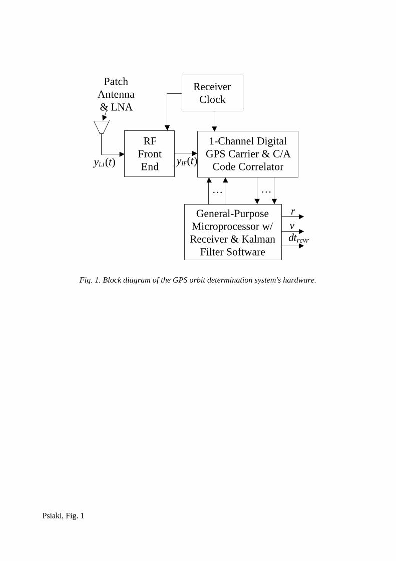
basic hardware components and their interactions are shown in Fig. 1. The signal yL1(t) is the GPS

L1 signal, and yIF(t) is a down-converted version of this signal that has been band-pass filtered, re-

scaled, and digitized.

The microprocessor must multi-task a number of different software processes. It uses three

broad categories of software: the signal acquisition, tracking, and data demodulation software, the

software that schedules which satellite to track, and the orbit determination Kalman filter software.

The acquisition, tracking and demodulation software operates much like that of a normal

receiver except for one significant difference: The signal acquisition process is assumed to be

aided by the Kalman filter. Aiding gives the acquisition a good estimate of a signal's Doppler

shift, which reduces the required time to lock onto a signal. The overall system's success is

dependent on its ability to acquire and lock onto a signal quickly. Throughout this study, it has

been assumed that signal lock can be achieved in 30 sec.

In LEO there will normally be a number of satellites in view, which is why it is necessary to

have a scheduling module that picks which satellite to track at any given time. A simple algorithm

has been used to accomplish this task. It uses three principal inputs. One input is the rough

ephemeris data for the entire GPS constellation, which is located in an almanac that is resident in

6

the microprocessor's memory. Another input is the Kalman filter's estimate of the satellite

position. The third input is the target nominal tracking interval for a single satellite.

The tracking selection algorithm operates as follows. It allows the receiver to track a

particular GPS satellite's signal until the target tracking duration has been achieved or until the

signal's SNR becomes too low to maintain lock. It then cycles through the list of satellite pseudo-

random number (PRN) codes in the order of ascending PRN identifier (ID) numbers. It selects the

next available satellite that, according to the constellation almanac and the estimated user

spacecraft location, should be in view with sufficiently high SNR to allow tracking (≥ 37 dB Hz).

This SNR calculation takes into account the gain pattern of each GPS satellite's L1 antenna,

occultation of the signal by the Earth, the gain pattern of the user antenna, and an estimate of the

user spacecraft attitude. The list of PRN ID numbers is repeated cyclically in the scheduler. After

the visible GPS satellite with the highest PRN ID number has been tracked, the algorithm starts

over again at the bottom of the list. If the only visible satellite is the one that is already being

tracked, then the scheduling algorithm will re-select the currently tracked satellite. In this case, the

receiver will continue to track the current satellite for longer than the target interval.

The Kalman filter estimates the spacecraft's position and velocity and corrections to the

receiver clock. It operates on pseudo-range data, time data, and possibly carrier phase data. This

data is provided by the digital correlator. The filter also needs to know the ephemeris and the

clock corrections for the tracked GPS satellite. This data is provided by the demodulation

software, which decodes the GPS signal's navigation message. Each signal must be tracked for at

least 30 seconds so that the full navigation message can be decoded.

Kalman Filter Design

The Kalman filter that is used in this system is a sampled-data extended Kalman filter that

7

stores its state estimate and state error covariance in the Square-Root Information Filter (SRIF)

format. The SRIF for linear discrete-time systems is described in Ref. 9, and an extension to

handle nonlinear sampled-data systems is described in Ref. 10.

Two modifications of the basic filter algorithm have been used for the problem at hand. One

allows it to append the carrier phase ambiguity state for the tracked satellite onto the state vector

at the start of a tracking interval and to delete it from the state vector at the end of the interval. The

other modification is to include the option to use a nonlinear iteration in the measurement update in

order to aid convergence from large initial errors. Both of these modifications are described later

in this section.

State Vector and Dynamic Model. The filter operates on a state vector, alternatively

propagating it between measurement sample times based on a dynamic model and then updating it

using the measured data in conjunction with a measurement model. This filter's state vector is:

x =

jNftvr

rcvr

rcvrδδ (1)

where x is the 9×1 state vector, r is the 3×1 Cartesian position vector of the user spacecraft in

Earth-Centered Inertial coordinates (ECI), v is the 3×1 Cartesian velocity vector of the user

spacecraft in ECI coordinates, δtrcvr is the receiver clock error, δfrcvr is the receiver frequency error

expressed as a fraction of its nominal frequency, and N j is the carrier phase ambiguity for GPS

satellite j, which is the currently tracked satellite. The state vector gets shortened to an 8×1 vector

by deletion of N j whenever the receiver is not tracking a GPS signal.

Before developing a dynamic model of the system, one needs to know the relationship

8

between the receiver clock's time and true GPS time, which is Universal time plus a few leap

seconds. Suppose that t is the true GPS time and that trcvr is the receiver clock's estimate of t. Then

the relationship between these two times and the receiver clock error is

t = trcvr - δtrcvr (2)

The filter uses a nonlinear differential equation to model the system's dynamics. It

numerically integrates this equation between sample intervals in order to develop an equivalent

nonlinear discrete-time difference equation of the system. The differential equation model of this

system is expressed using trcvr as its independent variable. This is necessary because the system

keeps track of events using trcvr. If one uses the prime notation (') to denote differentiation with

respect to trcvr, then the system's differential equation model is:

r' = v [1 – (δfrcvr + wt)] (3a)

v' = [g(r) + adrag(r,v;CDS/m) + wv] [1 – (δfrcvr + wt)] (3b)

(δtrcvr)' = δfrcvr + wt (3c)

(δfrcvr)' = wf (3d)

(N j)' = 0 for any j (3e)

The function g(r) is the gravitational acceleration, and the function adrag(r,v;CDS/m) is the

aerodynamic drag acceleration. The parameters CD, S, and m are, respectively, the drag

coefficient, the aerodynamic reference area, and the mass of the user spacecraft. The 3×1 vector

wv(t) is a white-noise process disturbance; it is the unmodeled component of the user spacecraft's

acceleration. The first two equations model the user spacecraft's point-mass translational

kinematics and its F=ma dynamics. The third and fourth equations model the receiver clock's

drift 11. The scalars wt(t) and wf(t) are white-noise process disturbances that drive the drift model.

9

The last equation expresses the fact that the carrier phase ambiguity is constant during a given

tracking interval.

The white noise inputs are uncorrelated with each other, and their statistics are given by:

E{wv(t)} = 0, E{wv(t)wvT(τ)} = Qvδ(t - τ) (4a)

E{wt(t)} = 0, E{wt(t)wt(τ)} = 0.5h0δ(t - τ) (4b)

E{wf(t)} = 0, E{wf(t)wf(τ)} = 2π2h-2δ(t - τ) (4c)

where Qv is a 3×3 positive definite matrix and h0 and h-2 are positive scalars that Ref. 11 uses to

quantify oscillator stability.

The gravity model g(r) only includes the 1/||r||2 central force and the J2 oblateness effect.

This simplification reduces the computational load of the filter, but it also impacts the filter’s

performance. The philosophy of this design is to minimize the computational load while still

maintaining a certain level of estimation accuracy. As will be seen in the results section, this

modeling simplification can be tolerated in LEO, but it causes serious problems at higher altitudes,

when there are long data gaps during which no GPS satellites are visible. A more accurate gravity

model could improve the performance in such cases, but no such model is considered for use in

this Kalman filter because the goal is to design a relatively simple estimation system.

The drag model adrag(r,v;CDS/m) uses a logarithmic interpolation of the 1976 U.S. Standard

Atmosphere 12 to derive density. It computes the drag based on the assumption that the atmosphere

is at rest with respect to the Earth. An a priori modeled value is used for the inverse ballistic

coefficient, CDS/m.

Measurement Model. Two types of position measurements are available from a typical

GPS receiver. One is pseudo range, ρ j. It is the distance from the user spacecraft to tracked GPS

spacecraft j as determined by the time of flight of the radio signal. The time of flight is based both

10

on the receiver clock, which is inaccurate, and on GPS satellite j's clock, which is very accurate.

A mathematical model for this measurement is

ρ j = )()( jj rrrr T −− + cδtrcvr + nρ (5)

where rj is the position of GPS satellite j in ECI coordinates at the time that the signal left the

satellite, c is the speed of light in vacuum, and nρ is the pseudo range measurement error. The

vector rj can be derived from the decoded navigation message. The measurement error is

composed of several constituents: ionospheric delay, GPS satellite ephemeris and clock errors,

and receiver generated noise 13. Multi-path error, although significant in terrestrial pseudo-range

measurements, is probably not a significant error source for spacecraft. The filter assumes that the

pseudo range measurement error is a discrete-time white-noise process with zero mean and a

standard deviation of σρ.

The other available measurement is the phase of the carrier signal, φ j. If the phase is

measured in cycles, then its mathematical measurement model is

λL1φ j = )()( jj rrrr T −− + cδtrcvr - N j + nφ (6)

where λL1 = 19.03 cm is the carrier wavelength of the L1 signal and nφ is the carrier phase

measurement error. The significant components of the carrier phase measurement error are

ionospheric phase advance, user-spacecraft-generated multi-path reflections, and receiver

generated noise. Similar to the pseudo range error, this error source is assumed to be a discrete-

time white-noise process with zero mean and a standard deviation of σφ. This filter assumes that

nρ and nφ are uncorrelated. Strictly speaking, this is not true; the ionospheric components of the

two measurement errors are negatively correlated with a correlation coefficient of -1.

11

Comments About the Use of the Carrier Phase Measurement. It should be noted that the

consideration of carrier phase measurements in this study is unusual. Carrier phase is normally

used only in precise orbit determination systems that often can track 4 or more GPS satellites

simultaneously and that use differential corrections from ground-based receivers 4,14. The use of

carrier phase for stand-alone civilian systems was considered to be pointless when Selective

Availability (SA) was in effect because SA dominated both σρ and σφ and made them equivalent

for long tracking intervals. Now that SA has been turned off, σφ is likely to be much smaller than

σρ (except for the constant average of its ionospheric component, which can be treated as part of N

j). This opens up the possibility that carrier phase may improve the accuracy of a stand-alone

civilian system. For example, carrier phase may improve the velocity estimation accuracy.

Two versions of the filter have been developed in order to evaluate whether carrier phase

measurements provide any benefit. One version uses carrier phase, as already described, and the

other does not. This second filter provides a benchmark for assessing the benefits of carrier data.

There are a few fine points about how best to fold the carrier phase ambiguity into and out of

the state vector at the beginning and end of a tracking interval. Reference 4 appends the ambiguity

to the state vector and initializes its variance to an artificially high value. There is a more exact

way to do this in the context of an SRIF. The procedure of Ref. 4 is optimal in the limit as the

initial variance of the phase ambiguity approaches infinity. Unfortunately, in the context of a

Kalman filter that stores the state estimation error covariance matrix or its square root, it is not

possible to let the initial phase ambiguity variance actually go to infinity.

An SRIF allows one to exactly achieve an infinite initial variance for the carrier phase

ambiguity. The SRIF simply appends N j to the state vector and appends a column of zeros to its a

priori square root state information matrix. This operation exactly achieves an infinite initial

12

variance because an SRIF stores square roots of information matrices instead of covariance

matrices, and a covariance of infinity corresponds to an information value of 0. The appended

column of zeros poses no problem to the SRIF because, after a measurement update has been

performed, the a posteriori square root information matrix becomes nonsingular.

The SRIF design makes it slightly more difficult to delete the ambiguity at the end of a given

satellite’s tracking interval. A standard covariance representation can simply delete the ambiguity

from the state vector while simultaneously deleting the corresponding rows and columns from the

state estimation error covariance matrix. The SRIF algorithm must first isolate the phase

ambiguity in its state information equation. Suppose that the state information equation takes the

form:

R x = z - n (7)

where R is the square root information matrix, z is a vector that stores an equivalent of the current

state estimate, and n is a zero-mean, unit-variance, uncorrelated random error vector. Note that R-

1z is the state estimate and that R-1(R-1)T is the state estimation error covariance matrix. Orthogonal

factorization must be used to isolate the phase ambiguity in the R matrix. This is accomplished by

using a Householder orthonormal transformation, H, to transform R so that the last column of Rtr =

HR, the column associated with N j, has zeros in all of its entries below the first row. If the vector

z also gets transformed, ztr = Hz, then the correct square root information matrix after the deletion

of Nj is Rtr with its first row and last column deleted, and the corresponding vector is ztr with its

first row deleted.

Note that there are other possible ways to make use of carrier phase data. For example, one

could implement carrier smoothing of the pseudo-range measurements. The philosophy of this

13

design is to make optimal use of both the carrier phase measurements and the filter’s dynamic

model. This is the same philosophy as has been adopted in Ref. 4.

System Observability. The observability of this system has been checked. The

observability analysis calculates the system's observability Gramian for a linearization of the

dynamics and measurement equations about the estimated state time history. The Gramian has been

calculated for an observation vector that includes all of the carrier phase ambiguities for all of the

GPS satellites that get tracked during the interval of interest. The Gramian must be nonsingular in

order for observability to hold 15.

The system has been found to be observable for representative LEO cases. The Gramian

starts out being singular because the system initially tracks only one GPS spacecraft, but by the

time it has locked on to the fourth spacecraft, the Gramian is clearly nonsingular.

Iterated Nonlinear Measurement Update. It is sometimes useful to use a special form of

the SRIF measurement update that employs nonlinear least squares methods. This procedure

amounts to an SRIF implementation of what is commonly known as an iterated extended Kalman

filter. Suppose that the a priori state error information equation is R~ x = z~ - n~ . Then the

solution of the following nonlinear least-squares problem constitutes the nonlinear measurement

update:

14

find: x (8a)

to minimize: JLS = 0.5 ( R~ x - z~ )T( R~ x - z~ )

+ 221

ρσ[ )()( jj rrrr T −− + cδtrcvr - ρ j]2

+ 22

1

φσ[ )()( jj rrrr T −− + cδtrcvr - N j - λL1φ j]2 (8b)

This nonlinear least squares problem can be solved using an iterative numerical optimization

procedure such as the Gauss-Newton method 16. As a point of reference, the standard (i.e., non-

iterated) measurement update of an extended Kalman filter can be viewed as being a single Gauss-

Newton step starting from an initial guess equal to the a priori state estimate. Two Gauss-Newton

steps are used in this paper's iterated filter, and the first step starts from the a priori state estimate.

The iterated update uses an adaptive step size algorithm that approximately minimizes the

least-squares function along each Gauss-Newton search direction 16. Adaptive step size methods

are known to improve convergence robustness in the general field of nonlinear optimization. The

same holds true in the case of iterated extended Kalman filtering. The improved ability to

converge can be significant when the filter starts with a poor initial state estimate.

Filter Tuning. Proper tuning of the filter is necessary in order to achieve reasonable

accuracy. The filter gets tuned by selection of its initial a priori state estimation error square root

information matrix and by selection of its process and measurement noise intensities, Qv, h0, h-2, σρ

and σφ.

The initial state estimation error variances, whose inverse square roots are the diagonal

elements of the initial square root information matrix, have been sized to reflect the statistics of the

actual errors between the filter's initial state estimate and the initial state of the truth model. This

assumes that the user has a good idea of the accuracy of the initial state estimate.

15

Similarly, the clock drift intensities, h0 and h-2, have been selected to be the same as are used

in the truth model. This assumes that the user has tested the receiver clock and characterized its

stability by selecting appropriate values of these two parameters.

The intensity of the acceleration process noise, Qv, has been sized based on the expected

level of the acceleration error in the filter’s models and based on the expected average time

interval that the receiver needs in order to have tracked 4 different GPS satellites. This time

interval has been chosen for the heuristic reason that 4 is the minimum number of GPS signals

needed for standard point positioning. This method of tuning effectively tells the filter to wait until

it sees 4 GPS satellites before it decides to attribute a measurement anomaly to the effects of

unmodeled accelerations.

These considerations lead to the following method of picking Qv. Suppose that the average

interval for tracking a total of 4 GPS satellites is ∆t4 and that the expected level of acceleration

uncertainty in the filter model is aerr. Then the matrix Qv is set equal to the identity matrix times the

constant 0.25(aerr)2∆t4. In low Earth orbits the acceleration errors are dominated by uncertainty in

the Earth gravity model, and the value aerr = 10-4 m/sec2 is a reasonable measure of this uncertainty.

If ∆t4 = 300 sec, then Qv = 7.5×10-7×I in units of m2/sec3. In practice, values within a factor of 3 of

this value have all yielded fairly similar performance for LEO cases. This tuning value is

reasonable for any orbit in the altitude range from 350 km up to 3200 km.

For altitudes above 3,200 km the tuning becomes more difficult because ∆t4 can become very

large due to gaps in the coverage of the GPS constellation. There do not seem to be any good rules

of thumb for such cases. Values on the order of Qv = 3×10-8×I m2/sec3 have given the best results

in GEO, and values on the order of 10-7×I m2/sec3 have worked reasonably well in highly elliptical

orbits that spend some time below 3,200 km altitude and much more time above that altitude.

16

The last two tuning parameters are the measurement noise intensities, σρ and σφ. These

quantities are tuned partly based on a priori measurement error estimates and partly based on the

receiver's measured SNR and known tracking loop bandwidths. The receiver can monitor the

SNR of the 1000 Hz accumulations that its digital correlator chip produces, and it can use this

SNR to predict the noise contributions to the pseudo range and carrier phase measurement errors.

These noise contributions are then RSS'd (root-sum-squared) with a priori measurement error

standard deviations to produce σρ and σφ.

In the case of σρ, the largest contributor to its a priori component is the anticipated

ionospheric error. Estimates for this error range from a root-mean-square (RMS) value of about 3

or 4 m at a 350 km altitude down to less than 1 m at a 1000 km altitude. In GEO, the RMS

ionospheric error is likely to be large, perhaps as much as 10 m, because a given GPS satellite is

visible to the user satellite only when the line of sight vector between them passes near the Earth,

and therefore, through a significant portion of the ionosphere. For an elliptical orbit, the expected

ionospheric error component at its lowest altitude is used to tune σρ. Note that the numbers quoted

here come from an approximate ionospheric model that will be described later in this paper.

These values assume that the receiver does not compensate for ionospheric effects.

The a priori component of σφ has been sized based on the expected levels of carrier phase

multi-path error from reflections off of the user spacecraft. These have been sized conservatively

at 0.010 m based on information given in Ref. 17.

III. Truth Model Simulation for Use in Filter Evaluation

Philosophy of Truth Model Filter Evaluation. The truth model generates data for use in

evaluating the filter. It simulates GPS tracking data, the truth position and velocity states of the

user spacecraft, and the truth states of the GPS receiver's clock error. Its dynamics and

17

measurement models incorporate effects that are not included in the filter. The filter processes the

simulated tracking data and produces estimates of the position, velocity, and clock error states.

The filter performance can be measured by comparison of these estimates to their truth-model

counterparts. In addition, the filter's tuning can be evaluated for rough consistency by comparing

the statistics of the “actual” errors to the predicted error variances that the filter computes in its

normal course of operation.

Dynamics Truth Model. The truth dynamic model is like that given in eqs. (3a)-(3e), but

with 4 differences: First, the gravity model includes a 30×30 spherical harmonic expansion of the

Earth’s gravity field and Solar and Lunar point-mass effects. The coefficients of the Earth gravity

model are those of NASA’s EGM 96 model 18. Second, an acceleration due to solar radiation

pressure is included. It produces accelerations on the order of 10-7 m/sec2 during orbit day. Third,

the truth drag model uses different values of (CDS)/m than are used by the filter. The filter's

(CDS)/m values have errors that range from –40% to +67% of the truth model values. Fourth, the

random white-noise acceleration error in eq. (3b), wv, is eliminated.

The dominant discrepancy between the truth orbital dynamics model and the filter’s orbital

dynamics model is the difference in their gravity fields. This is true at all altitudes down to the

lowest altitude of interest, 350 km. In LEO orbits the resulting acceleration differences are on the

order of 10-4 m/sec2 and are due to non-spherical Earth effects. In GEO orbits the differences are

mainly due to Solar and Lunar gravity effects and are on the order of 10-5 m/sec2.

The simulation uses a discrete-time random sequence from a random number generator in

order to simulate the effects of the process noise terms that drive the receiver clock drift, wt and wf.

Two different clock stability truth models have been used in this study. One has drift parameters

representative of a temperature-compensated crystal oscillator: h0 = 2×10-19 sec and

18

h-2 = 2×10-20 /sec 11. Throughout the remainder of this paper, this clock model is referred to as the

TCXO. The drift parameters of the other model roughly correspond to those of an ovenized crystal

oscillator that is currently in use in a space-based GPS receiver: h0 = 2×10-22 sec and h-2 = 6.1×10-

22 /sec. This more stable receiver clock model is referred to as the OXO throughout the remainder

of this paper.

Measurement Truth Model. The simulation's measurement model is based on eqs. (5) and

(6). It uses the dynamic model's truth values for r and δtrcvr in these equations. The value of N j is

chosen arbitrarily so that the measured φ j = 0 at the start of a tracking interval. The complicated

parts of the measurement truth model lie in its calculation of the GPS satellite position, r j, the

pseudo range error, nρ, and carrier phase measurement error, nφ.

The truth model simulation actually computes two values of the GPS satellite position. One

is the truth value that it uses in the measurement equations, and the other is a reported value that it

sends to the receiver via its navigation message. The truth value of r j is obtained using the Yuma

almanac for week 9 19. The reported value is produced using ephemerides that are slightly

perturbed from the truth ephemerides. These perturbations produce RMS position errors for the

GPS satellites on the order of 3 m over a 12 hour period, which is consistent with experimentally

obtained results 20.

The simulated measurement errors are sums of several components. One is a random

component that is based on the SNR of the received signal and on the receiver's tracking loop

bandwidth. The bandwidths of the carrier and code tracking loops have both been fixed at 1 Hz.

The received SNR is computed by taking actual experimental data from a typical roof top patch

antenna and scaling it based on the differing distance from the user satellite to the GPS satellite

and based on the location of the user satellite in the GPS satellite's antenna gain pattern. The user

19

satellite's antenna gain pattern also is considered, but only as a go/no-go criterion that checks

whether the GPS satellite is within the presumed 65 deg half width of the gain pattern's conical

FOV. The noise-induced pseudo-range measurement errors are no more than 2 m RMS in GEO,

and they get as low as 0.5 m RMS in LEO. The noise component of the carrier phase error is

extremely low, ranging from 1×10-4 m RMS in LEO to 4×10-4 m RMS in GEO.

Another component of the measurement error truth model is an ionospheric model. This

model is a modified version of the ionospheric correction model that is commonly used in single-

frequency receivers 21. It incorporates an altitude dependence of the electron density that has a

scale height of 120 km below 1000 km of altitude, and a scale height of 2000 km above this

altitude. The ionospheric delay is computed from this model by integrating along the line of sight

from the user spacecraft to the tracked GPS satellite. This ionospheric delay is then multiplied by

the speed of light. The resultant distance is added to nρ to model the code delay and subtracted

from nφ to model the carrier phase advance.

Another component of both measurement errors is the residual clock error of the tracked

GPS satellite. This has been modeled as a second-order polynomial that varies slowly. The range

equivalent error can have a magnitude as large as 4 m, and each satellite's clock error can vary by

as much as 1.5 range-equivalent meters in a day.

The final simulated measurement error is the carrier phase multi-path error. This error is

modeled as being a function of the orientation in user spacecraft coordinates of the line of sight

vector to the tracked GPS satellite. The attitude of the user satellite is assumed to be nadir-

pointing. The multi-path error function is defined by a random, but constant, spherical harmonic

expansion of up to 7th degree. Two different multi-path models have been used. They both have

20

maximum carrier phase multi-path errors of 0.01 m, which is consistent with results reported in

Ref. 17.

IV. Simulation-Based Performance Evaluation of the System

A Typical LEO Case. The following example is representative of many LEO cases. The

spacecraft orbit has an apogee altitude of 656 km, a perigee altitude of 607 km, and an inclination

of 58 deg. The receiver clock is the TCXO. The Kalman filter processes one measurement

sample every 15 seconds. The receiver nominally tracks one new GPS satellite every 75 sec. The

first 45 seconds of this period are spent acquiring the signal, and the last 30 seconds are spent

tracking it, which yields 3 actual measurements per satellite. If the SNR becomes too low to

maintain lock before the signal has been tracked for 30 seconds, then the data are discarded under

the assumption that the receiver may have failed to decode the full navigation message. The

Kalman filter uses the carrier phase data, but does not use the iterated measurement update.

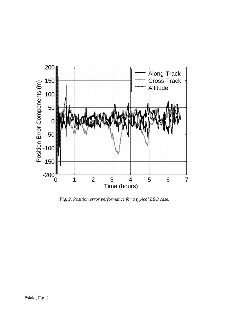
Figure 2 shows the position error time history for this case broken into its three components,

along-track (the solid curve), cross-track (the dash-dotted curve), and altitude (the dotted curve).

The initial position error is 15 km, and the initial velocity error is 17 m/sec. As shown in the

figure, the filter quickly converges from these initial errors to reach an accuracy of better than 200

meters in the first tenth of an hour. This is the time that is required to finish tracking 4 GPS

satellite signals and to start on the 5th. This rapid convergence illustrates the fact that the system’s

observability has mostly to do with how many GPS satellites the receiver tracks in a given time

period. The filter takes about half an hour to settle into steady-state operation. The peak steady-

state errors for this case are 64 m along-track, 128 m across-track, and 72 m in altitude. The

corresponding RMS component errors are 19 m, 42 m, and 23 m.

21

This represents a significant performance degradation in comparison to a multi-channel

receiver. A benchmark simulation of a 12-channel receiver operating in point-solution mode has

been run for all cases that have been considered in this paper. In the case that corresponds to Fig.

2, the point solution achieves peak position errors of 5 m along-track, 5 m across-track, and 13 m

in altitude. The corresponding RMS position errors are, respectively, 1.4 m, 1.7 m, and 3.5 m.

Thus, the proposed system’s accuracy is about an order of magnitude worse than that of the

standard multi-channel point solution. This level of performance differential between the two

systems is typical of many LEO cases.

The proposed system would be useful for many missions despite this degraded performance.

Many spacecraft require orbit determination accuracy on the order of 100 to 200 m. This paper’s

system would serve the needs of such spacecraft at a reduced level of power consumption.

The present system compares favorably with the microGPS receiver of Ref. 7. The position

accuracies of the two systems are similar, but the time transfer accuracy of the present system is

much better, on the order of 10-6 sec vs. 0.05 sec for the microGPS system.

The position errors for this case have been compared to the filter’s predicted standard

deviations for these quantities. On average, the statistics of the along-track and altitude errors

agree fairly well with the filter’s modeled statistics, but the RMS cross-track error is almost 3

times larger than its predicted value. Although obviously sub-optimal, this is a tolerable level of

statistical mis-match, which is why the filter performs reasonably well.

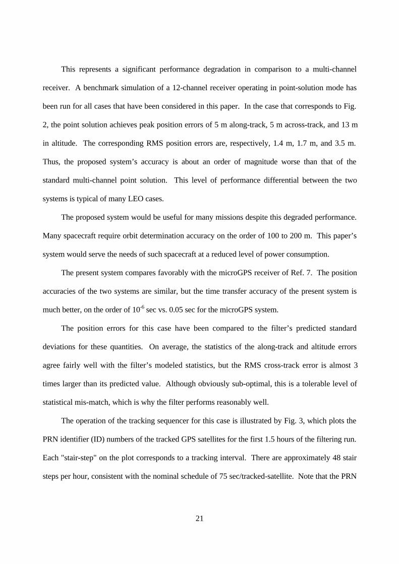
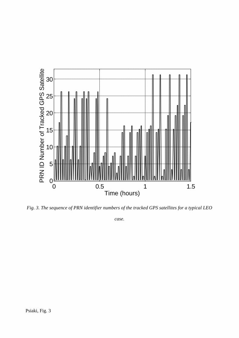
The operation of the tracking sequencer for this case is illustrated by Fig. 3, which plots the

PRN identifier (ID) numbers of the tracked GPS satellites for the first 1.5 hours of the filtering run.

Each "stair-step" on the plot corresponds to a tracking interval. There are approximately 48 stair

steps per hour, consistent with the nominal schedule of 75 sec/tracked-satellite. Note that the PRN

22

ID sequence follows a cyclical pattern: the numbers increase monotonically for sub-sequence

lengths of between 2 and 6 tracking intervals until they approach the highest available PRN ID

number, 31. Then the sequence drops down to a low PRN ID number to start a new cycle. Two

important points to notice are the lack of data gaps and the fact that most of the adjacent groups of

4 ID numbers correspond to 4 different GPS satellites. These two characteristics are important to

achieving good observability of the system and, therefore, good accuracy. These characteristics

are typical for LEO.

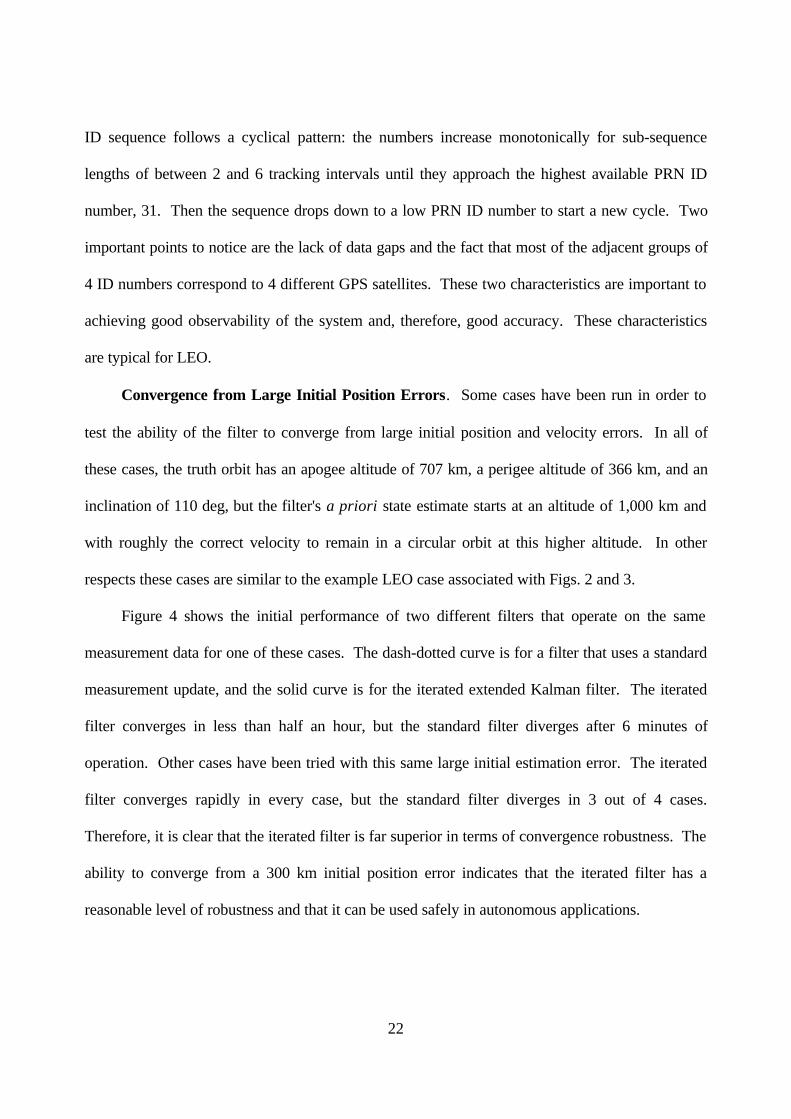
Convergence from Large Initial Position Errors. Some cases have been run in order to

test the ability of the filter to converge from large initial position and velocity errors. In all of

these cases, the truth orbit has an apogee altitude of 707 km, a perigee altitude of 366 km, and an

inclination of 110 deg, but the filter's a priori state estimate starts at an altitude of 1,000 km and

with roughly the correct velocity to remain in a circular orbit at this higher altitude. In other

respects these cases are similar to the example LEO case associated with Figs. 2 and 3.

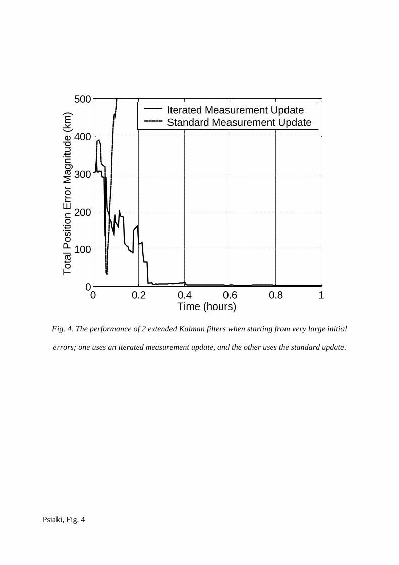
Figure 4 shows the initial performance of two different filters that operate on the same

measurement data for one of these cases. The dash-dotted curve is for a filter that uses a standard

measurement update, and the solid curve is for the iterated extended Kalman filter. The iterated

filter converges in less than half an hour, but the standard filter diverges after 6 minutes of

operation. Other cases have been tried with this same large initial estimation error. The iterated

filter converges rapidly in every case, but the standard filter diverges in 3 out of 4 cases.

Therefore, it is clear that the iterated filter is far superior in terms of convergence robustness. The

ability to converge from a 300 km initial position error indicates that the iterated filter has a

reasonable level of robustness and that it can be used safely in autonomous applications.

23

Performance as a Function of Orbit. A number of orbital inclinations, eccentricities, and

altitudes have been investigated. The only orbital parameter that has a significant impact on

system performance is altitude. The dominant altitude impact comes if the orbit extends above the

altitude 3,200 km, at which point there start to be long gaps when there are no GPS signals

available because the user spacecraft passes outside of the primary gain pattern of the GPS

satellites’ broadcast antennas.

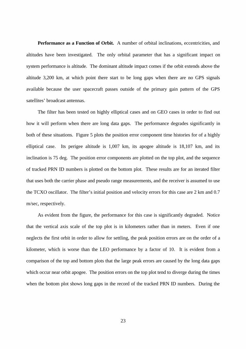
The filter has been tested on highly elliptical cases and on GEO cases in order to find out

how it will perform when there are long data gaps. The performance degrades significantly in

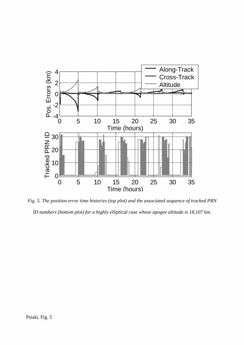
both of these situations. Figure 5 plots the position error component time histories for of a highly

elliptical case. Its perigee altitude is 1,007 km, its apogee altitude is 18,107 km, and its

inclination is 75 deg. The position error components are plotted on the top plot, and the sequence

of tracked PRN ID numbers is plotted on the bottom plot. These results are for an iterated filter

that uses both the carrier phase and pseudo range measurements, and the receiver is assumed to use

the TCXO oscillator. The filter’s initial position and velocity errors for this case are 2 km and 0.7

m/sec, respectively.

As evident from the figure, the performance for this case is significantly degraded. Notice

that the vertical axis scale of the top plot is in kilometers rather than in meters. Even if one

neglects the first orbit in order to allow for settling, the peak position errors are on the order of a

kilometer, which is worse than the LEO performance by a factor of 10. It is evident from a

comparison of the top and bottom plots that the large peak errors are caused by the long data gaps

which occur near orbit apogee. The position errors on the top plot tend to diverge during the times

when the bottom plot shows long gaps in the record of the tracked PRN ID numbers. During the

24

low-altitude portions of the orbit, however, the accuracy of this case is comparable to that of the

LEO cases.

The system performance is even further degraded in GEO. The best GEO results that have

been achieved exhibit peak errors on the order of 7 km. The OXO had to be used for the

receiver’s oscillator in order to achieve even this poor level of performance – the filter has a

tendency to diverge if the TCXO is used in GEO. The poorer GEO performance is the result of the

very long data gaps that occur regularly at these high altitudes. The average time that is required in

order to see 4 different GPS signals is on the order of 4 hours. It is difficult to improve the GEO

performance by going to a multi-channel receiver because there are very few times when more

than one GPS satellite signal is available with sufficient strength to be tracked by a conventional

receiver 22.

It should be noted that the GEO case is the only one for which a large performance

improvement has been realized through use of the OXO as the receiver clock. The LEO cases and

the elliptical case show only moderate improvements from using the OXO.

A secondary altitude effect is present for LEO cases. For altitudes below 3,200 km there is

a slight degradation in accuracy with a decrease in altitude. For example, a case with a perigee

altitude of 985 km and an apogee altitude of 1007 km experienced a peak altitude error of 100 m.

The peak altitude error increased to 144 m when the perigee and apogee altitudes decreased to

357 km and 375 km, respectively. This modest performance degradation with decreases in

altitude is probably the result of errors in the filter’s orbital dynamics model. The model neglects

Earth gravity terms above J2, and the strength of these terms increases as altitude decreases.

The Effect of Inaccuracy in the Filter’s Orbital Dynamics Model. An improvement in the

accuracy of the filter’s dynamics model can significantly improve its performance. This has been

25

demonstrated by tests in which the dynamic modeling mis-match between the truth model and the

filter has been reduced to about 10-7 m/sec2. In GEO this reduces the peak steady-state position

error from 7 km to about 400 m. The peak errors are reduced from about 100 m to about 20 m in

LEO. In order to achieve these improvements in the LEO cases, one would have to add a

significant number of terms to the filter’s spherical harmonic expansion of the Earth’s gravitational

field. In GEO one would have to include Solar and Lunar gravity models.

These approaches run counter to this system’s philosophy of reducing computational load. If

one needs more accuracy in LEO, then perhaps one should go to a multi-channel receiver. In GEO,

however, a conventional multi-channel receiver will not be of much help, and one may be forced

to make the requisite improvements in the dynamics model.

The Usefulness of Carrier Phase Measurements. This study has considered whether the

use of carrier phase measurements in the Kalman filter improves this system's performance. The

answer is: definitely not. The use of carrier phase data has not yielded consistent accuracy

improvements in the cases that have been considered. In fact, the filter that does not use carrier

phase sometimes performs better than the one that uses it.

Dependence of Performance on Miscellaneous Filter/Receiver Properties. There are

additional system design parameters that affect accuracy. The use of longer tracking intervals for

individual GPS signals leads to a degradation of accuracy in LEO cases. For example, if one uses

300 sec per tracked signal as opposed to this study's nominal value of 75 sec, then the LEO

accuracy degrades by a factor of about 2 to yield peak per-axis errors on the order of 230 m and

per-axis RMS errors on the order of 60-70 m. This fact suggests that it would be a good idea to

shorten the nominal tracking interval to something less than 75 sec. Unfortunately, there is a limit

26

to how much one can shorten this interval due to the need to allow adequate time for acquisition

and due to the need to decode the 30 sec navigation message.

There is some evidence that use of a shorter sample interval, 5 sec as opposed to 15

seconds, may slightly improve performance. This change also triples the computational cost of the

filter. The possibility of modest improvements is probably not worth the cost of switching to the

shorter sampling period.

Computational Burden of Kalman Filter. In most cases considered, the Kalman filter

requires an average computation rate of less than 3,000 floating point operations per second

(flops/sec). This figure encompasses all propagation and measurement update operations,

including numerical integration of the equations of motion. It corresponds to a 15 second

measurement sample period with one 4th/5th-order Runge-Kutta numerical integration step per

sample interval. If carrier phase measurements are not used, then the computational cost gets

reduced by 5% to 10%. If the iterated nonlinear measurement update is used, then the

computational cost increases by about 10% and may be slightly more than 3,000 flops/sec. If the

sample interval gets reduced, then the computational cost increases in inverse proportion to the

interval's length. Note that the 3,000 flops/sec figure does not include the cost of the calculation of

GPS satellite locations from the ephemeris data.

Use of this system will provide tremendous savings in terms of computational cost. The

3,000 flops/sec figure is probably less than the cost of running the 1,000 Hz signal tracking loop

for a single channel of a normal receiver. Thus, if one reduces from a 10 channel receiver to a one

channel receiver, then the savings in carrier tracking alone will be on the order of 80% or more

even after one accounts for the added cost of running the Kalman filter. Furthermore, the reduction

from 10 channels to 1 channel implies that most other computations, such as the calculation of GPS

27

satellite locations, will be reduced by a factor of 10. Thus, the present system is expected to save

more than 80% of the total computational load. This savings will allow the use of a much slower

clock speed for the receiver’s microprocessor, which will translate proportionally into reduced

power consumption.

V. Summary and Conclusions

A new system has been proposed for doing autonomous orbit determination for Earth orbiting

spacecraft. It consists of a single channel GPS receiver coupled to an extended Kalman filter. The

receiver tracks a different GPS satellite once every 75 seconds and sends pseudo range

measurements to the Kalman filter along with the location of the tracked GPS satellite. The

Kalman filter processes these measurements sequentially to estimate the user spacecraft's position

and velocity along with the receiver clock's offset and drift rate. The Kalman filter relies on

dynamical models of the orbital motion and of the receiver clock drift in order to propagate its

estimates between samples. The filter uses a simple gravity model in its orbit propagation, one

that includes only the 1/r2 and J2 terms. One version of the filter uses an iterated nonlinear

measurement update in order to increase its domain of convergence.

The motivation for examining this system has been to try to develop a low-power solution to

the autonomous orbit determination problem. A single-channel receiver can use a slower

microprocessor clock speed, which reduces its power consumption proportionally.

This system has been evaluated using a simulation study. The results are as follows: In low

Earth orbit the system can operate successfully using a low-power temperature-compensated

crystal oscillator for its receiver clock. The iterated version of the filter can reliably converge

from initial position errors as large as 300 km. Peak steady-state per-axis position errors ranging

from 78 m to 144 m can be achieved in low-Earth orbit. At geosynchronous altitudes the system

28

works poorly even when it incorporates an ovenized crystal oscillator. Its peak per-axis position

error can be as large as 7 km in this case. This poor performance is caused by two factors: the

limited availability of strong GPS signals at geosynchronous altitudes and the filter’s neglect of

Solar and Lunar gravity terms in its orbital dynamics model.

Acknowledgments

This work was supported in part by NASA through Grant Number NAG5-8788. Seymor

Kant was the NASA grant monitor. Hee Jung, a graduate student at Cornell, helped to develop the

code for the truth-model simulation’s spherical harmonic expansion of the Earth’s gravitational

field.

References

1. Hofmann-Wellenhof, B., Lichtenegger, H., and Collins, J., GPS, Theory and Practice,

Springer-Verlag, (New York, 1997), pp. 181-183.

2. Wertz, J.R., and Larson, W.J., eds., Space Mission Analysis and Design, Kluwer, (Boston,

1999), pp. 409-418.

3. Akos, D.M., Normark, P.-L., Enge, P., Hansson, A., and Rosenlind, A., “Real-Time GPS

Software Radio Receiver,” Proceedings of the ION National Technical Meeting, Institute of

Navigation (Alexandria, Virginia, 2001), pp. unnumbered.

4. Wu., S.C., Yunck, T.P., and Thornton, C.L., “Reduced-Dynamic Technique for Precise Orbit

Determination of Low Earth Satellites,” Journal of Guidance, Control, and Dynamics, Vol.

14., No. 1, 1991, pp. 24-30.

5. Yunck, T.P., Bertiger, W.I., Wu, S.C., Barsever, Y.E., Christensen, E.J., Haines, B.J., Lichten,

S.M., Muellerschoen, R.J., Vigue. Y., and Willis, P., “1st Assessment of GPS-Based Reduced

Dynamic Orbit Determination on TOPEX POSEIDON,” Geophysical Research Letters, Vol.

29

21, No. 7, 1994, pp. 541-544.

6. Chao, C.C. and Bernstein, H., “Onboard Stationkeeping of Geosynchronous Satellites Using a

Global Positioning System Receiver,” Journal of Guidance, Control, and Dynamics, Vol. 17.,

No. 4, 1994, pp. 778-786.

7. Reichert, A., Axelrad, P., Wu, S.C., Bertiger, W., and Srinivasan, J., "Initial Demonstration of

a Point Solution Algorithm for Orbit Determination Using the MicroGPS Receiver,"

Proceedings of the National Technical Meeting, Institute of Navigation, Jan. 14-16, 1997,

pp. 377-386.

8. Moreau, M., Axelrad, P., Garrison, J.L., Kelbel, D., and Long, A., "GPS Receiver Architecture

and Expected Performance for Autonomous GPS Navigation in Highly Eccentric Orbits,"

Proceedings of the ION 55th Annual Meeting, June 28-30, 1999, Cambridge, MA, pp. 653-

665.

9. Bierman, G.J., Factorization Methods for Discrete Sequential Estimation, Academic Press,

(New York, 1977), pp. 69-76, 115-122.

10. Psiaki, M.L., Theiler, J., Bloch, J., Ryan, S., Dill, R.W., and Warner, R.E. “ALEXIS

Spacecraft Attitude Reconstruction with Thermal/Flexible Motions Due to Launch Damage”,

Journal of Guidance, Control, and Dynamics, Vol. 20, No. 5, 1997, pp. 1033-1041.

11. Brown, R.G. and Hwang, P.Y.C., Introduction to Random Signals and Applied Kalman

Filtering, 3rd Edition, J. Wiley & Sons, (New York, 1997), pp. 428-432.

12. Anon., U.S. Standard Atmosphere, 1976, National Oceanic and Atmospheric Administration,

1976.

13. Parkinson, B.W., "GPS Error Analysis," in Global Positioning System: Theory and

Applications, Vol. I, Parkinson, B.W. and Spilker, J.J. Jr., eds., American Institute of

30

Aeronautics and Astronautics, (Washington, 1996), pp. 469-483.

14. Yunck, T.P., "Orbit Determination," in Global Positioning System: Theory and Applications,

Vol. II, Parkinson, B.W. and Spilker, J.J. Jr., eds., American Institute of Aeronautics and

Astronautics, (Washington, 1996), pp. 559-592.

15. Kailath, T., Linear Systems, Prentice-Hall, (Englewood Cliffs, N.J., 1980), pp. 615-618.

16. Gill, P.E., Murray, W., and Wright, M.H., Practical Optimization, Academic Press, (New

York, 1981), pp. 88-93, 134-136.

17. Cohen, C.E., "Attitude Determination," in Global Positioning System: Theory and

Applications, Vol. II, Parkinson, B.W. and Spilker, J.J. Jr., eds., American Institute of

Aeronautics and Astronautics, (Washington, 1996), pp. 519-538.

18. Anon., “EGM96, The NASA GSFC and NIMA Joint Geopotential Model,”

http://cddisa.gsfc.nasa.gov/926/egm96/egm96.html, NASA Goddard Space Flight Center,

Greenbelt, Maryland, 2001.

19. Anon., "GPS Almanacs," U.S. Coast Guard Navigation Center, http://www.navcen.uscg.mil/

gps/almanacs, May 2000.

20. Zumberge, J.F. and Bertiger, W.I., "Ephemeris and Clock Navigation Message Accuracy," in

Global Positioning System: Theory and Applications, Vol. I, Parkinson, B.W. and Spilker,

J.J. Jr., eds., American Institute of Aeronautics and Astronautics, (Washington, 1996), pp. 585-

599.

21. Klobuchar, J.A., "Ionospheric Effects on GPS," in Global Positioning System: Theory and

Applications, Vol. I, Parkinson, B.W. and Spilker, J.J. Jr., eds., American Institute of

Aeronautics and Astronautics, (Washington, 1996), pp. 485-515.

31

22. Long, A., Kelbel, D., Lee, T., Garrison, J., and Carpenter, J.R., "Autonomous Navigation

Improvements for High-Earth Orbiters Using GPS," Paper no. MS00/13, Proceedings of the

15th International Symposium on Spaceflight Dynamics, CNES, June 26-30, 2000, Biarritz,

France, pp. unnumbered.

Figure captions.

Fig. 1. Block diagram of the GPS orbit determination system's hardware.

Fig. 2. Position error performance for a typical LEO case.

Fig. 3. The sequence of PRN identifier numbers of the tracked GPS satellites for a typical LEO

case.

Fig. 4. The performance of 2 extended Kalman filters when starting from very large initial errors;

one uses an iterated measurement update, and the other uses the standard update.

Fig. 5. The position error time histories (top plot) and the associated sequence of tracked PRN ID

numbers (bottom plot) for a highly elliptical case whose apogee altitude is 18,107 km.

Psiaki, Fig. 1

Fig. 1. Block diagram of the GPS orbit determination system's hardware.

vδtrcvr

yL1(t)

PatchAntenna& LNA

RFFrontEnd

1-Channel DigitalGPS Carrier & C/A

Code CorrelatoryIF(t)

General-PurposeMicroprocessor w/Receiver & Kalman

Filter Software

…

ReceiverClock

r

…

Psiaki, Fig. 2

Fig. 2. Position error performance for a typical LEO case.

0 1 2 3 4 5 6 7-200

-150

-100

-50

0

50

100

150

200

Time (hours)

Pos

ition

Err

or C

ompo

nent

s (m

)

Along-TrackCross-TrackAltitude

Psiaki, Fig. 3

Fig. 3. The sequence of PRN identifier numbers of the tracked GPS satellites for a typical LEO

case.

0 0.5 1 1.50

5

10

15

20

25

30

Time (hours)

PR

N ID

Num

ber o

f Tra

cked

GP

S S

atel

lite

Psiaki, Fig. 4

Fig. 4. The performance of 2 extended Kalman filters when starting from very large initial

errors; one uses an iterated measurement update, and the other uses the standard update.

0 0.2 0.4 0.6 0.8 10

100

200

300

400

500

Time (hours)

Tot

al P

ositi

on E

rror

Mag

nitu

de (k

m) Iterated Measurement Update

Standard Measurement Update

Psiaki, Fig. 5

Fig. 5. The position error time histories (top plot) and the associated sequence of tracked PRN

ID numbers (bottom plot) for a highly elliptical case whose apogee altitude is 18,107 km.

0 5 10 15 20 25 30 35-4

-2

0

2

4

Time (hours)

Pos

. Err

ors

(km

) Along-TrackCross-TrackAltitude

0 5 10 15 20 25 30 350

10

20

30

Time (hours)

Tra

cked

PR

N ID