shodhganga.inflibnet.ac.inshodhganga.inflibnet.ac.in/bitstream/10603/7499/14/14_chapter 4.pdf · C or ec t md lf ps a ynbv ix w h unacceptable assumptions. The classical modeling

�

�

�

�

� �

��

��

Chapter 4 Soft Computing: Techniques and Development Tools

67

Chapter gives a brief overview of the computing techniques such as Fuzzy logic, Neural

Network, Neuro-Fuzzy networks and GA. The most popular tools used by the researchers for

development and simulation study of the system under test such as MATLAB, SIMULINK and

associated tool boxes for software development and testing are also described.

4.1 Soft Computing Traits

• Fuzzy logic [1] is derived from fuzzy set theory dealing with reasoning that is approximate rather

than precisely deduced from classical predicate logic. It can be thought of as the application side of

fuzzy set theory dealing with well thought out real world expert values for a complex problem In

this context, FL is a problem-solving control system methodology that lends itself to

implementation in systems ranging from simple, small, embedded micro-controllers to large,

networked, multi-channel PC or workstation-based data acquisition and control systems.

• Neural Network [2] almost all information-processing needs of today are met by digital

computers. So we can consider their possibility of information processing techniques that are

different from those used in conventional digital computers. Neural networks are constructed with

neurons that connected to each other. There are many types of neural networks for various

applications in the literature. A common used one of these is multilayered perceptrons (MLP)

• Genetic Algorithm (GAs) [3], which uses the concept of Darwin’s theory, have been widely

introduced to deal with nonlinear control difficulties and to solve complicated optimization

problems. Darwin’s theory basically stressed the fact that the existence of all living things is based

on the rule of ’survival of the fittest’. In the theory of evolution, different possible solutions to a

problem are selected first to a population of binary strings encoding the parameter space. The

selected solutions undergo a parallel global search process of reproduction, crossover and mutation

to create a new generation with the highest fitness function

• Neuro-Fuzzy [4] ANFIS uses a hybrid learning algorithm to identify the membership function

parameters of single-output, Sugeno type fuzzy inference systems (FIS). A combination of least-

squares and back-propagation gradient descent methods are used for training FIS membership

function parameters to model a given set of input/output data. This is the major training routine for

Sugeno-type fuzzy inference systems.

• Genetic Algorithms (GAs) are robust, numerical search methods that mimic the process of

natural selection. Although not guaranteed to absolutely find the true global optima in a defined

search space, GAs are renowned for finding relatively suitable solutions within acceptable time

frames and for applicability to many problem domains [5]. During the last decade, GAs has been


68

applied in a variety of areas, with varying degrees of success within each. A significant

contribution has been made within control systems engineering. GA exhibit considerable

robustness in problem domains that are not conducive to formal, rigorous, classical analysis

• Evolutionary computation (EC) [6] is field of methods of problem-solving developed by

computer scientists which tries to emulate the process of biological evolution to generate fitter

solutions from the available ones. Evolution can be viewed as a two-step iterative process,

consisting of random variation followed by selection. EC is a broad category, which includes

mainly Genetic Algorithms (GAs) [7], Evolution strategies and some non-genetic approaches.

When applied to problem-solving evolutionary algorithms result in extremely optimization

procedures which are relatively free from some of the most cumbersome problems of traditional

optimization – especially the necessity to make definite assumptions about how to evaluate the

fitness of a solution. For example, for applying Linear Programming, the cost function should be

linear, or, for gradient based methods it should be smooth and differentiable. EC can be applied

without such constraints. Hence, a broad range of problems which are outside the range of

conventional engineering and numerical techniques, become amenable to EC. EC is also yielding

some exiting results in generating intelligence in the form of learning systems. The learning, which

can be accomplished by the conventional well-established AI techniques like Expert Systems, is

limited by the knowledge of the designer. In other words the ES can’t become smarter than its

creator can’t. Whereas EC in conjunction with ANN and Fuzzy logic based approaches have

resulted in the creation of systems, which could become more intelligent than their designers by

learning from experience.

4.2 Soft Computing: Introduction Correct model of process may not be available or mode may be complex with too many

unacceptable assumptions. The classical modeling algorithm may not respond well to the measurement

noise in sensors or performance through classical algorithms may not be adequate. The FUZZY LOGIC based systems may be developed to overcome classical algorithm problems.

The fuzzy logic frees us from the true/false reasoning of logical system of type that is used in symbolic

languages.

Fuzzy linguistic models [8] hold the promise of providing a finite qualitative partition of a

quantitative dynamic system while being applicable to any system that can be described in linguistic

terms. Fuzzy models provide a succinct and robust representation of systems that lack a complete

quantitative model or have uncertain system perturbations. Consistency in reasoning, however, has not yet

been proven for a fuzzy linguistic representation of a quantitative system.


69

Fuzzy linguistic models use fuzzy sets to create a finite number of partitions MBF of the inputs,

outputs and states of a quantitative system. Currently most fuzzy models are implemented as a set of if-

then rules, where the system input is used to evaluate the rules’ antecedents and the model’s output is the

combined output of all the rules evaluated in parallel. This simple logical system, a Fuzzy Inference

System (FIS), does not implement inference chaining and can only evaluate a simplified qualitative

model of a plant. Recent work has expanded the usefulness of this structure by providing machine

learning methodologies to adapt and tune fuzzy linguistic models and to automatically generate new

models through self-organization [8].

Input output relations (mapping) in the form of traditional mathematical modeling is replaced by

ANN learning the synaptic weights by undergoing a training process. ANN has built in adaptability or can

be trained to modify the weights with the change in environment [9]. The ANN can deal naturally with

contextual information. Since knowledge is represented by the regular structure and activation state of

network. Every neuron is potentially affected by the global activity of all other neurons. ANN can be

trained to make decisions and they are also fault tolerant in the sense that if a neuron or connecting link is

damaged, recalling a pattern will be impaired in quality but due to distribution of information in the

network damage has to be extensive for overall degradation. Since neurons are the common ingredients

for all ANN, it is possible to Share the algorithm and structures in different applications. So it is possible

to have a seamless integration of modules. The ANN is suitable in the following situation….

Learning or tuning allows the initial linguistic fuzzy model developed from heuristic domain

knowledge to be optimized. Learning is achieved by using a Neuro-Fuzzy structure and exploiting the

supervised learning strategies originally developed for neural networks.

These strategies include gradient descent back-propagation, least-mean-squares, and a hybrid

methodology that combines least-squares to optimize linear parameters and back-propagation to optimize

the nonlinear parameters. These same supervised learning methodologies can automatically learn any

arbitrary nonlinear mapping between input and output without an initial linguistic fuzzy model. The

resulting self-organized fuzzy models do not necessarily have a linguistic interpretation that would be

recognized by a human expert. Often systems developed through self-organization are never interpreted

linguistically, but are utilized effectively for pattern matching and curve fitting. Fuzzy networks are often

preferred for curve fitting because the fuzzy rules used by the network have only a local effect, in effect

providing an adaptive mechanism for implementing B-splines.

It is possible to integrate the fuzzy logic controller with ANN so that the expression for the

knowledge used in the systems is understood by humans. This reduces difficulties in describing the ANN.

Fuzzy controller learns to improve its performance using ANN structure & thus learns by Experience.

Neuro-computing is fast compared to conventional computing because of massive parallel computation.


70

Besides, it has the properties of fault tolerance and noise filtering. Here neural network is used as if

estimator. Neural network-based control strictly does not need a mathematical model of a plant like a

conventional control method does with the required precision.

4.3 Fuzzy Logic Fuzzy logic has rapidly become one of the most successful of today's technologies for developing

sophisticated control system. Fuzzy logic is nothing but the extension of binary logic. The main

difference between the Fuzzy logic and binary logic is that in binary logic we take only two cases,

either 0 or 1, that means low or high states. In Fuzzy Logic we take each & every state into

consideration. Fuzzy logic is a method for represent ting information in a way that resembles natural

human communication. It then manipulates that information similar to human reasoning. Fuzzy logic

has been applied to problems that are either difficult to tackle mathematically or where the use of fuzzy

logic provides improved performance. The development of fuzzy logic traces back to 1965 when Dr.

Lotfi Zadeh presented a paper on Fuzzy sets. Since, then this Fuzzy logic as a tool has come in long

way [10].

4.3.1 Keywords, Terminology

• Definition

Fuzzy Logic is the logic using fuzzy set defined by membership functions in the logical

expression corresponding to the rule base.

• Linguistic Variables

The primary building block of any fuzzy system is linguistic variable while the linguistic

term indicate / represent possible values of a linguistic variable. The linguistic variables

translate crisp value into a linguistic description.

• Fuzzy Set

A set obtained by assigning fuzzy values to the linguistic variable using

membership function.

• Premise

It is the fuzzy specification of linguistic variable.

• Conclusion

Fuzzy output in terms of linguistic variable is called conclusion.


71

• Fuzzy Rule A linguistic rule derived from the expert’s behavior to control process under

study. It contains premise as first part and conclusion as second part.

• Universe Of Discourse Universe of discourse is defined as the total range of all available information in a given

problem. Once this universe of discourse is known, we can define certain events on this

information space.

• Crisp And Fuzzy sets Crisp sets or classical sets contain information whether it belongs to the set or not. It is

very much same as digital logic or Boolean logic. Fuzzy sets on the other hand contain

information for which belongings varies from [0,1].This is therefore multi-valued logic.

• Membership Functions A membership function (MBF) is a curve that defines how each point in input space is

mapped to a membership value (or degree of membership) between 0 and 1. The simplest MF

is formed using straight lines. Simplest is the triangular MBF, a collection of three points

forming a triangle. Other types include the Trapezoidal, Sigmoidal, pi, Bell shape MBF.

• Fuzzification It is the process of assigning fuzzy values to linguistic variables using fuzzy set. In

the real world, hardware such as a digital voltmeter generates crisp data, but these data are

subjected to experimental error. We want to compare a crisp voltage reading to fuzzy sets

say as 'low voltage' or 'high voltage'. The range of the output voltage becomes the universe

of discourse and the process of identifying a crisp quantity as a fuzzy is called Fuzzification.

Assigning of range of membership to the transferred fuzzy quantity in this way is termed as

"Fuzzy Measures'. The assignment process can be intuitive, heuristic or it can be based upon

the algorithms or logical operations. Fuzzification is the first step where a crisp input is

fuzzified.

• Rule Base Creation Perhaps the most common way to represent knowledge is to form it into natural

language expression of the type.

If premise (antecedent), Then conclusion (consequent)

An inference such that if we know a fact (premise, hypothesis, and antecedent) then we

can either infer or derive another fact called conclusion (consequent). This form of knowledge is

quite appropriate in the content of linguistics as it expresses human empirical and heuristic

knowledge in our own language of communication. Collection of such rules forms a rule base.


72

The dimensions of rule base are dependent upon the fuzzification level of inputs. It is important

to note that all the inputs need not condition the output. One input may have an influence on the

output independent of other input. The formation of rule is a copyright process of the designer.

The process of combining the effect of these rules to produce an output is called as the process of

inference.

• Fuzzy Inference The fuzzy inference process consists of two phases:

1. The composition of rules applied.

2. Obtaining crisp output from fuzzy inference.

Task of meaningful combination of control actions prescribed by different rules

activation or firing is called as composition.

• Defuzzification

It is a process of rounding off from multi-valued output to a single value output.

The output of a fuzzy process can be the logical union of two or more fuzzy

Membership function defined on the universe of discourse of output variable. The

Choice of methods is again context dependent. The general criteria are that the method

must have continuity, unambiguity and computational simplicity. The centroid method

correctly fits into these requirements and almost invariably used.

4.3.2 Architecture of Fuzzy Inference System

The architecture of FIS is shown in Figure 4.1.

Figure 4.1: The Architecture of Fuzzy Inference System


73

The knowledge base contains information about the boundaries of the linguistic

variables data base. Fuzzification interface receives the current I/P value, maps it to a

suitable domain i.e. it converts the value to a linguistic term /Fuzzy set. Decision logic

determines the O/P value from the measured I/P according to the knowledge base. De-

fuzzification interface has the task of determining the crisp value. The design steps [11]

are as follows:

I. Create linguistic variables and vocabulary for the I/P-O/P variables in

which the rules of operation are specified.

II. With reference to the I/P-O/P and control variables, define the structure of

the system to represent the flow within a system.

III. Formulate the strategy as fuzzy rules, based on sound Egg. Judgment.

IV. Evaluate rule for current situation to obtain fuzzy output.

V. Use any of the Defuzzification technique to obtain crisp value.

4.4 Artificial Neural Network Almost all information-processing needs of today are met by digital computers. So we can

consider their possibility of information processing techniques that are different from those used in

conventional digital computers. Research is being vigorously pursued concerns the possibility of building

information processing devices that mimic the structures and operation principles commonly found in

humans and other living creatures, which has produced a new breed of computers called Neuro-

computers.

Neural computing is a new approach to information processing. It is the fast, vital alternative to

normal sequential processing. The large computing power lies in parallel processing architecture. It is

capable of imitating brain’s ability to make decisions and draw conclusions when presented with

complex, noisy, irrelevant or partial information. Thus it is the domain in which an attempt is made to

make compute think, react and compute.

Neurons are nerve cells and neural networks are networks of these cells. Thus they are one of a

group of intelligent technologies for data analysis that differ from other classical analysis techniques by

learning about user’s chosen subject from the data user provides them, rather than being programmed by

the user in a traditional sense. Neural networks gather their knowledge by detecting the patterns and

relationships in user’s data, learning from relationships and adapting to change.


74

“A neural network is a massively parallel distributed processor that has a natural propensity for

storing experiential knowledge and making it available for use. It resembles the brain in two respects:

• Knowledge is acquired by the network through a learning process.

• Interneuron connections strengths known as synaptic weights are used to store knowledge.

The interconnection architecture can be very different for different networks. Architectures can

vary from feed forward and recurrent structures to latticed structures.

An artificial neuron is a concept whose components have a direct analogy with the biological

neuron [12]. The structure of an artificial neuron is like an analog summer-like computation. It is also

called a neuron, PE (processing element), neuron, node, or cell. The input signals X1, X2, X3, … Xn are

normally continuous variables but can also be discrete pulses. Each input signal flows through a gin or

weight, called a synaptic weight or connection strength, whose function is analogous to that of the

synaptic junction in a biological neuron. The weights can be positive (excitory) or negative (inhibitory),

corresponding to “acceleration” or “inhibition,” respectively, of the flow of electrical signals in a

biological cell. The summing node accumulates all the input weighted signals, adds the bias signal b,

and then passes to the output through the activation function, which is usually nonlinear in nature.

Mathematically, the output expression can be given as,

� � �� (4.1)

Where Xi = inputs

Wi = weights b = bias

4.4.1 The Basic Artificial Model An artificial neuron is defined as follows:

It receives a number of inputs either from original data, or from the output of other neurons in the

neural network. Each input comes via a connection that has strength (weight); these weights correspond

to synaptic efficacy in a biological neuron. Each neuron also has a single threshold value. The weighted

sum of the inputs is formed, and the threshold subtracted, to compose the activation of the neuron (also

known as the post-synaptic potential, or PSP, of the neuron) [13].

The activation signal is passed through an activation function (also known as a transfer function)

to produce the output of the neuron. Inputs and outputs correspond to sensory and motor nerves such as


75

those coming from the eyes and leading to the hands. There can be hidden neurons that play an internal

role in the network. The input, hidden and output neurons need to be connected together.

Figure 4.2 shows the basic and simple model of an Artificial Neuron present in the layers of the

Artificial Neural Network.

Figure 4.2: Simple model of an Artificial Neuron

A simple network has a feed forward structure; signals flow from inputs, forwards through any

hidden units, eventually reaching the output units. Such a structure has stable behavior. However, if the

network is recurrent (contains connections back from later to earlier neurons) it can be unstable, and has

very complex dynamics.

When the network is executed (used), the input variable values are placed in the input units, and

then the hidden and output layer units are progressively executed. Each of them calculates its activation

value by taking the weighted sum of the outputs of the units in the preceding layer, and subtracting the

threshold. The activation value is passed through the activation function to produce the output of the

neuron. When the entire network has been executed, the outputs of the output layer act as the output of

the entire network.

4.4.2 Implementation of Artificial Neural Network The specification and design of an ANN application should aim to produce the best system and

performance overall. This means that conventional methods should be used if and where possible and

ANNs are used to supplement them or only if they can add some benefit. A neural network design

involves at least five main tasks: � Data collection.

� Raw data preprocessing.

� Feature extraction from preprocessed data.


76

� Selection of an ANN type and topology (architecture).

� ANN training, testing and validation.

4.4.3 Single layer and multi-layer networks

For single layer neural network, the output signals of the neurons in the first layer are the output

signals of the network. Here each neuron adjusts its weights according to what output was expected of it,

and the output it gave. The Perceptron Delta Rule can mathematically express this:

∆wi = xiδ (4.2)

Where, δ = (desired output) - (actual output).

This is of no use though when you extend the network to multiple layers to account for non-

linearly separable problems. When adjusting a weight anywhere in the network, we have to be able to tell

what effect this will have on the overall effect of the network. To do this, we have to look at the

derivative of the error function with respect to that weight.

Multi layer perceptrons are feed forward nets with one or more layers of nodes between the input

and output nodes. Multilayer feed forward networks normally consist of three or four layers; there is

always one input layer and one output layer and usually one or more hidden layers. The term input layer

neurons are a misnomer; no sigmoid unit is applied to the value of each of these neurons. Their raw

values are fed into the layer downstream the input layer (the hidden layer). Once the neurons for the

hidden layer are computed, their activations are then fed downstream to the next layer, until all the

activations eventually reach the output layer, in which each output layer neuron is associated with a

specific classification category. In a fully connected multilayer feed forward network, each neuron in one

layer is connected by a weight to every neuron in the layer downstream it. Thus in computing the value of

each neuron in the hidden and output layers one must first take the sum of the weighted sums and the

bias(if any) and then apply f(sum)(the sigmoid function) to calculate the neuron’s activation[14].

The capabilities of multi layer perceptrons stem from the nonlinearities used within nodes. The

number of nodes must be large enough to form a decision region that is as complex as is required by a

given problem. It must not, however, be so large that the many weights required cannot be reliably

estimated from the available training data. For example, two nodes are sufficient to solve the exclusive

OR problem.


77

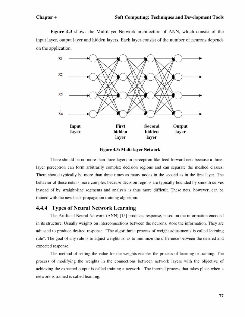
Figure 4.3 shows the Multilayer Network architecture of ANN, which consist of the

input layer, output layer and hidden layers. Each layer consist of the number of neurons depends

on the application.

Figure 4.3: Multi-layer Network

There should be no more than three layers in perceptron like feed forward nets because a three-

layer perceptron can form arbitrarily complex decision regions and can separate the meshed classes.

There should typically be more than three times as many nodes in the second as in the first layer. The

behavior of these nets is more complex because decision regions are typically bounded by smooth curves

instead of by straight-line segments and analysis is thus more difficult. These nets, however, can be

trained with the new back-propagation training algorithm.

4.4.4 Types of Neural Network Learning The Artificial Neural Network (ANN) [15] produces response, based on the information encoded

in its structure. Usually weights on interconnections between the neurons, store the information. They are

adjusted to produce desired response. “The algorithmic process of weight adjustments is called learning

rule”. The goal of any rule is to adjust weights so as to minimize the difference between the desired and

expected response.

The method of setting the value for the weights enables the process of learning or training. The

process of modifying the weights in the connections between network layers with the objective of

achieving the expected output is called training a network. The internal process that takes place when a

network is trained is called learning.


78

�� Supervised learning

Supervised learning is a process of training a neural network by giving it examples of the task we

want it to learn. i.e. it is a learning with a teacher. The way this is done is by providing a set of pairs of

vectors (patterns), where the first pattern of each pair is an example of an input pattern that the network

might have to process and the second pattern is the output pattern that the network should produce for that

input which is known as a target output pattern for whatever input pattern.

Thus, supervised leaning means “a learning process in which, change in a network's weights and

biases are due to the intervention of any external teacher. The teacher typically provides output targets.”

This technique is mostly applied to feed forward type of neural networks

During each learning or training iteration the magnitude of the error between the desired and

actual network response is computed and used to make adjustments to the internal network parameters or

weights according to some learning algorithm. As the learning proceeds, the error is gradually reduced

until it achieves a minimum or at least and acceptably small value.

Sometimes if it is not require computing exact error between the desired and the actual network

response, and for each training example the network is given a pass/fail signal by the teacher, then it is

called Reinforcement learning which is a special type of supervised learning. If a fail is assigned, the

network continues to readjust its parameters until it achieves a pass or continues for a predetermined

number of tries, whichever comes first.

�� Unsupervised learning

It is the learning process in which changes in a network's weights and biases are not due to the

intervention of any external teacher. Commonly changes are a function of the current network input

vectors, output vectors, and previous weights and biases.

The network is able to discover statistical regularities in its input space and automatically

develops different modes of behavior to represent different classes of inputs (in practical applications

some labeling is required after training, since it is not known at the outset which mode of behavior will be

associated with a given input class). In this type of learning due to absence of desired output it is difficult

to predict what type of features network will extract. Although learning in these nets can be slow, running

the trained net is very fast - even on a computer simulation of a neural net. Table gives comprehensive

summary of techniques.


79

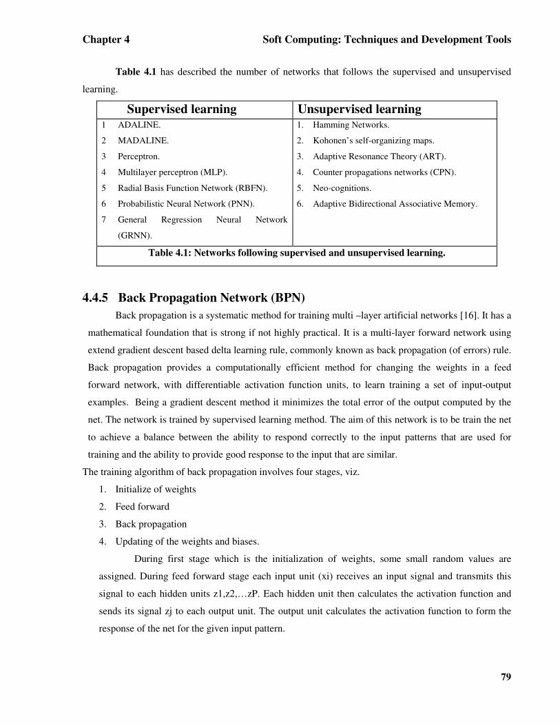
Table 4.1 has described the number of networks that follows the supervised and unsupervised

learning.

Supervised learning Unsupervised learning 1 ADALINE.

2 MADALINE.

3 Perceptron.

4 Multilayer perceptron (MLP).

5 Radial Basis Function Network (RBFN).

6 Probabilistic Neural Network (PNN).

7 General Regression Neural Network

(GRNN).

1. Hamming Networks.

2. Kohonen’s self-organizing maps.

3. Adaptive Resonance Theory (ART).

4. Counter propagations networks (CPN).

5. Neo-cognitions.

6. Adaptive Bidirectional Associative Memory.

Table 4.1: Networks following supervised and unsupervised learning.

4.4.5 Back Propagation Network (BPN) Back propagation is a systematic method for training multi –layer artificial networks [16]. It has a

mathematical foundation that is strong if not highly practical. It is a multi-layer forward network using

extend gradient descent based delta learning rule, commonly known as back propagation (of errors) rule.

Back propagation provides a computationally efficient method for changing the weights in a feed

forward network, with differentiable activation function units, to learn training a set of input-output

examples. Being a gradient descent method it minimizes the total error of the output computed by the

net. The network is trained by supervised learning method. The aim of this network is to be train the net

to achieve a balance between the ability to respond correctly to the input patterns that are used for

training and the ability to provide good response to the input that are similar.

The training algorithm of back propagation involves four stages, viz.

1. Initialize of weights

2. Feed forward

3. Back propagation

4. Updating of the weights and biases.

During first stage which is the initialization of weights, some small random values are

assigned. During feed forward stage each input unit (xi) receives an input signal and transmits this

signal to each hidden units z1,z2,…zP. Each hidden unit then calculates the activation function and

sends its signal zj to each output unit. The output unit calculates the activation function to form the

response of the net for the given input pattern.


80

During back propagation of errors, each output unit compares its computed activation yk with

its target value tk to determine the associated error for that pattern with that unit. Based on the error,

the factor δk (k= 1,…m) is computed and is used to distribute the error at output unit yk back to all

units in the previous layer. Similarly, the factor δj (j=1,..p) is computed for each hidden unit zj.

During the final stage, the weight and biases are updated using the δ factor and the activation. During

final stage, the weight and biases are updated using δ factor and the activation.

�� Parameter x: Input training vector. t: output target vector

δk : error at output unit yk δj : error at hidden unit zj

α = learning rule Voj = bias on hidden unit j

zj= hidden unit j wok = bias output unit k

y = output unit k.

�� Initialization of weights Step: 1 Initialize weight to small random values.

Step: 2 while stopping condition is false, do steps 3-10

Step: 3 for each training pair do steps 4-9

�� Feed forward Step 4: Each input unit receives the input signal xi and transmits this signals to all units in the

layer above i.e. hidden units.

Step 5: Each hidden unit (zj, j = 1,..p) sums its weighted input signals

�=

− +=n

1iinj xivijvojz (4.3)

Applying activation function

)z(fZj inj= (4.4)

and sends this signal to all units in the layer above i.e. output units.

Step 6: Each output unit (yk, k = 1,..m) sums its weighted input signals

�=

− +=p

1jink zjwjkwoky (4.5)

And applies its activation function to calculate the output signals

)inky(fYk −= (4.6)


81

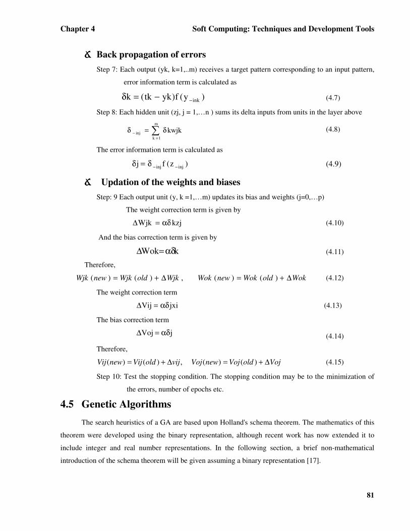
�� Back propagation of errors Step 7: Each output (yk, k=1,..m) receives a target pattern corresponding to an input pattern,

error information term is calculated as

)y(f)yktk(k ink−−=δ (4.7)

Step 8: Each hidden unit (zj, j = 1,…n ) sums its delta inputs from units in the layer above

�=

− δ=δm

1kinj kwjk (4.8)

The error information term is calculated as

)z(fj injinj −−δ=δ

(4.9)

�� Updation of the weights and biases Step: 9 Each output unit (y, k =1,…m) updates its bias and weights (j=0,…p)

The weight correction term is given by

kzjWjk αδ=∆ (4.10)

And the bias correction term is given by

kWok αδ=∆ (4.11)

Therefore,

WokoldWoknewWokWjkoldWjknewWjk ∆+=∆+= )()( ,)()( (4.12)

The weight correction term

jxiVij αδ=∆ (4.13)

The bias correction term

jVoj αδ=∆ (4.14)

Therefore,

VojoldVojnewVojvijoldVijnewVij ∆+=∆+= )()( ,)()( (4.15)

Step 10: Test the stopping condition. The stopping condition may be to the minimization of

the errors, number of epochs etc.

4.5 Genetic Algorithms The search heuristics of a GA are based upon Holland's schema theorem. The mathematics of this

theorem were developed using the binary representation, although recent work has now extended it to

include integer and real number representations. In the following section, a brief non-mathematical

introduction of the schema theorem will be given assuming a binary representation [17].


82

A schema (H) is defined as a template for describing a subset of chromosomes with similar

sections. The template consists of multiple 0's, 1's, and meta-characters or "don't care" symbols (#). The

meta-character is simply a notational device used to signify that either a 1 or 0 will match that pattern. For

example, consider a schema such as, #0000. This schema matches two chromosomes, 10000 and 00000.

The template is a powerful way of describing similarities among patterns in the chromosomes. The total

number of schemata present in a chromosome of length L is equal to 3L. According to Holland, the order

of a schema (o(H)) is equal to the number of fixed positions (i.e., non-meta-characters) and the defining

length of a schema (L(H)) is the total number of characters. Thus, the schema #00#0 is an order 3 schema

(o (H) = 3) and has a length of 5 (L(H) = 5). Holland derived an expression that predicts the number of

copies a particular schema, H, would have in the next generation after undergoing exploitation,

recombination and mutation. This expression is shown below

m(H,t+1) >= m(H,t) - f(H)/f [1 - (Pr(L(H)/(t-1))-o(H)Pm] (4.16)

where H is a particular schema, t is the generation, m(H,t+1) is the number of times a particular

schema is expected in the next generation, m(H,t) is the number of times the schema is in the current

generation, f(H) is the average fitness of all chromosomes that contain schema H, f is the average fitness

for all chromosomes, Pr is the probability of recombination occurring, and Pm is the mutation probability.

The primary conclusion that can be drawn from inspection of this equation is that as the ratio of f(H) to f

becomes larger, the number of the times H is expected in the next generation increases. Thus, particularly

good schemata will propagate in future generations.

Two more points need to be made concerning Holland's schema theorem. Although both mutation

and recombination destroy existing schemata, they are necessary for building better ones. The degree to

which they are destroyed is dependent upon the order (o(H)) and the length (L(H)) of the schemata. Thus,

schemata that are low-order, well-defined, and have above average fitness are preferred and are termed

"building blocks". This definition leads to the building block principle of GAs which states that “there is

a high probability that low-order; well-defined, average fitness schemata will combine through

recombination to form higher order, above average fitness schemata”. Recombination is critical

because it is the only procedure by which building blocks located on different sections of a chromosome

can be combined onto the same chromosome. By employing the concept of building blocks, the

complexity of the problem is reduced. Instead of trying to find a few large-order schemata by chance,

small pieces of the chromosome that are important (i.e., building blocks) are combined with other

important small pieces to produce over many generations an optimized chromosome. Because the GA has

the ability to process many schemata in a given generation, GAs are said to have the property of "implicit

parallelism", thereby making them an efficient optimization algorithm.


83

4.5.1 When to use genetic algorithms? When not much is known about the response surface and computing the gradient is either

computationally intensive or numerically unstable many scientists prefer to use optimization methods

such as genetic algorithms, simulated annealing, and Simplex optimization which do not require gradient

information. One of the reasons to use genetic algorithms is their versatility. Using the knowledge about

the system one can tailor the algorithm for a particular application. If the application calls for an

optimization method with hill-climbing characteristics the algorithm can be modified by using an elitist

strategy. If becoming trapped in local optima is a problem, mutation can be increased. Thus, while there is

no guarantee that GAs will perform the best for a particular application one can usually change some

aspect of the genetic configuration or use different genetic operator to achieve adequate search

performance.

Another feature about GAs that one can take advantage of is that GAs do not optimize directly on

the variables but on their representations.

For applications where the variables being optimized are very different from each other (i.e. a

mixture of integers, binary values, and floating points numbers).The GAs are an excellent choice for these

types of applications. The GA configuration can be modified to include different mutation operators for

different sections of the chromosome.

Genetic algorithms (GAs) are optimization techniques based on the concepts of natural selection

and genetics. In this approach, the variables are represented as genes on a chromosome. GAs features a

group of candidate solutions (population) on the response surface. Through natural selection and the

genetic operators, mutation and recombination, chromosomes with better fitness are found. Natural

selection guarantees that chromosomes with the best fitness will propagate in future populations. Using

the recombination operator, the GA combines genes from two parent chromosomes to form two new

chromosomes (children) that have a high probability of having better fitness than their parents. Mutation

allows new areas of the response surface to be explored. GAs offer a generational improvement in the

fitness of the chromosomes and after many generations will create chromosomes containing the optimized

variable settings. Genetic algorithms (GAs) are stochastic global search and optimization methods that

mimic the metaphor of natural biological evolution. GAs operates on a population of potential solutions

applying the principle of survival of the fittest to produce successively better approximations to a

solution. In this approach, the variables are represented as genes on a chromosome.

Through natural selection and the genetic operators, mutation and recombination, chromosomes

with better fitness are found.


84

At each generation of a GA, a new set of approximations is created by the process of selecting

individuals according to their level of fitness in the problem domain and reproducing them using

operators borrowed from natural genetics. This process leads to the evolution of populations of

individuals that are better suited to their environment than the individuals from which they were created,

just as in natural adaptation.

Natural selection guarantees that chromosomes with the best fitness will propagate in future

populations. Using the recombination operator, the GA combines genes from two parent chromosomes to

form two new chromosomes (children) that have a high probability of having better fitness than their

parents. Mutation allows new areas of the response surface to be explored. GAs offer a generational

improvement in the fitness of the chromosomes and after many generations will create chromosomes

containing the optimized variable settings.

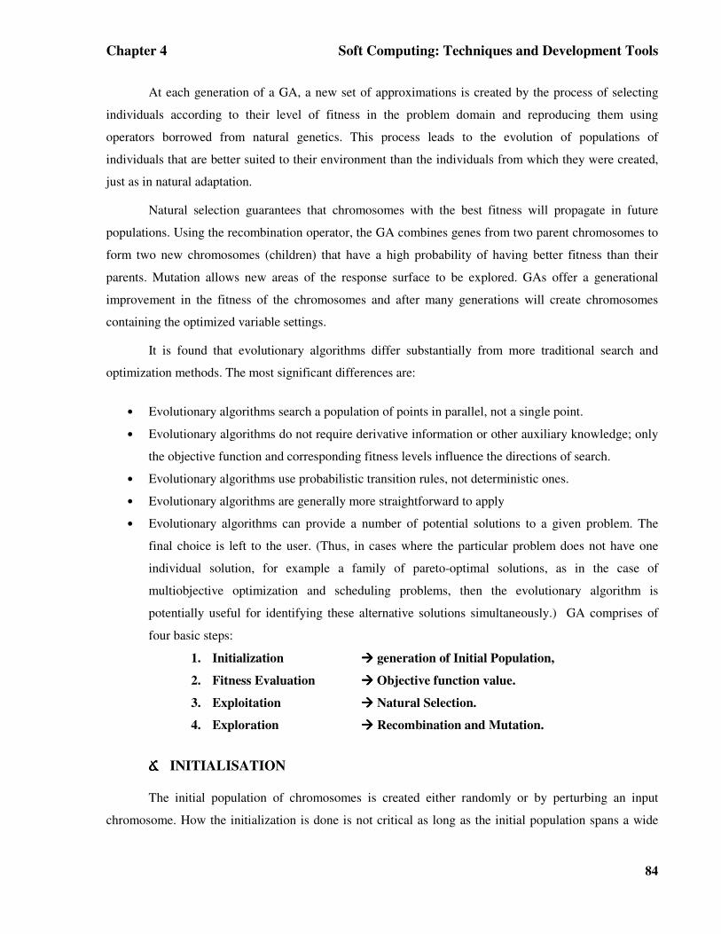
It is found that evolutionary algorithms differ substantially from more traditional search and

optimization methods. The most significant differences are:

• Evolutionary algorithms search a population of points in parallel, not a single point.

• Evolutionary algorithms do not require derivative information or other auxiliary knowledge; only

the objective function and corresponding fitness levels influence the directions of search.

• Evolutionary algorithms use probabilistic transition rules, not deterministic ones.

• Evolutionary algorithms are generally more straightforward to apply

• Evolutionary algorithms can provide a number of potential solutions to a given problem. The

final choice is left to the user. (Thus, in cases where the particular problem does not have one

individual solution, for example a family of pareto-optimal solutions, as in the case of

multiobjective optimization and scheduling problems, then the evolutionary algorithm is

potentially useful for identifying these alternative solutions simultaneously.) GA comprises of

four basic steps:

1. Initialization �� generation of Initial Population,

2. Fitness Evaluation �� Objective function value.

3. Exploitation �� Natural Selection.

4. Exploration �� Recombination and Mutation.

�� INITIALISATION

The initial population of chromosomes is created either randomly or by perturbing an input

chromosome. How the initialization is done is not critical as long as the initial population spans a wide


85

range of variable settings (i.e., has a diverse population). Thus, if we have explicit knowledge about the

system being optimized that information can be included in the initial population.

At the beginning of the computation a number of individuals (the population) are randomly

initialised. The first/initial generation is produced.

If the optimization criteria are not met the creation of a new generation starts. Individuals are

selected according to their fitness for the production of offspring. Parents are recombined to produce

offspring. All offspring will be mutated with a certain probability. The fitness of the offspring is then

computed. The offspring are inserted into the population replacing the parents, producing a new

generation. This cycle is performed until the optimization criteria are reached.

Such a single population evolutionary algorithm is powerful and performs well on a broad class

of problems. However, better results can be obtained by introducing many populations, called

subpopulations. Every subpopulation evolves for a few generations isolated (like the single population

evolutionary algorithm) before one or more individuals are exchanged between the subpopulations. The

Multipopulation evolutionary algorithm models the evolution of a species in a way more similar to nature

than the single population evolutionary algorithm.

�� FITNESS EVALUATION

In the second step, evaluation, the fitness is computed. It consists of the determination of the

objective function value of a particular chromosome. The goal of the fitness function is to numerically

encode the performance of the chromosome. For real-world applications of optimization methods such as

GAs the choice of the fitness function is the most critical step.

�� EXPLOITATION

The third step is the exploitation or natural selection step. In selection the individuals producing

offspring are chosen .Each individual in the selection pool receives a reproduction probability depending

on the own objective value and the objective value of all other individuals in the selection pool. In this

step, the chromosomes with the largest fitness scores are placed one or more times into a mating subset in

a semi-random fashion. Chromosomes with low fitness scores are removed from the population. There are

several methods for performing exploitation such as: Rank-based fitness assignment; Roulette wheel

selection ; Stochastic universal sampling; Local selection; Truncation selection and Tournament selection


86

�� EXPLORATION

It consists of the recombination and mutation operators.

Recombination: There are basically two types of recombination techniques.

• Real valued recombination

1 Discrete recombination

2 Intermediate recombination

3 Line recombination

4 Extended line recombination

• Binary valued recombination (crossover)

1 Single-point crossover

2 Multi-point crossover

3 Uniform crossover

4 Shuffle crossover

5 Crossover with reduced surrogate

Mutation: After recombination offspring undergo mutation. Offspring variables are mutated by the

addition of small random values (size of the mutation step), with low probability. The probability of

mutating a variable is set to be inversely proportional to the number of variables (dimensions). The

more dimensions one individual has as smaller is the mutation probability. There are different

reported results for the optimal mutation rate. According to one theory, the mutation rate of 1/n (n=

number of variables) produce good results for a broad class of test function. However, the mutation

rate was independent of the size of the population. For unimodal functions a mutation rate of 1/n is

the best choice. An increase of the mutation rate at the beginning connected with a decrease of the

mutation rate to 1/n at the end gives only an insignificant acceleration of the search. However, for

multimodal functions a self adaptation of the mutation rate could be useful.

Real valued mutation: The size of the mutation step is usually difficult to choose. The optimal step size depends

on the problem considered and may even vary during the optimization process. Small steps are often

successful, but sometimes bigger steps are quicker.

A proposed mutation operator (the mutation operator of the Breeder Genetic Algorithm):

• mutated variable = variable ± range·delta; (+ or - with equal probability)


87

• range = 0.5·domain of variable; (search interval),

• delta = sum(a(i) 2^-i), a(i) = 1 with probability 1/m, else a(i) = 0; m = 20.

This mutation algorithm is able to generate most points in the hypercube defined by the

variables of the individual and range of the mutation. However, it tests more often near the variable,

that is, the probability of small step sizes is greater than that of bigger steps With m=20, the mutation

algorithm is able to locate the optimum up to a precision of .(range·2^-19) .

Binary mutation: For binary valued individuals mutation means flipping of variable values. For every

individual the variable value to change is chosen uniform at random. Table 4.2 shows an example of

a binary mutation for an individual with 11 variables, variable 4 is mutated.

before mutation 0 1 1 1 0 0 1 1 0 1 0

after mutation 0 1 1 0 0 0 1 1 0 1 0

Table 4.2: Individuals before and after binary mutation

After the exploration step, the population is full of newly created chromosomes (children)

and steps two through four are repeated. This process continues for a fixed number of

generations.

4.5.2 GA Terminology

1. Chromosome Length is the number of genes present on the chromosome. The chromosome

length is an important consideration when optimizing a real variable problem. Longer

chromosomes allow better conversion from the binary chromosome to the real number variable.

However, the longer chromosome is computationally more inefficient and generally takes longer

to find the optimal region. This concept can be studied by changing the fitness function to the

bohachevsky function.

2. Population Size is the number of chromosomes in the population. Larger population sizes

increase the amount of variation present in the population at the expense of requiring more fitness

function evaluations. The best population size is dependent upon both the application and the

length of the chromosome. For longer chromosomes or more challenging the optimization

problems, I usually use of population size greater than 100, while for simpler problems a

population size of 20 will lead to good results.

3. Number of Generations is the maximum number of generations that will be performed.


88

4. Mutation Rate is the probability of mutation occurring. Mutation is the random flipping of one

of the bits or genes (i.e., change a 0 to 1). Mutation is employed to give new information to the

population. It also prevents the population from becoming saturated with chromosomes that all

look alike (premature convergence). Large mutation rates increase the probability of destroying a

good chromosome, but prevent premature convergence. The best mutation rate is application

dependent and related to both the length of the chromosome and the size of the population. For

most applications a mutation rate of 0.1 to 0.01 is employed.

5. Crossover Rate is the probability of crossover reproduction being performed. A high crossover is

used to encourage good mixing of the chromosomes. For most applications a crossover rate of

0.75 to 0.95 is employed.

6. Crossover Type is the type of crossover reproduction that is employed. The GA demo allows

three different types of crossover: single, double, and uniform. The choice of crossover type is

primarily application dependent.

7. Elitist Operator determines whether the best chromosome for each population is placed into the

next generation unchanged. Most applications that I have seen use some form of elitist operator.

If the elitist operator is turned on, the best fitness score from one population to the next will never

decrease.

8. Fitness Function allows the user to decide which fitness function the GA should employ. The

first fitness function is called the simple function and consists of the summation of the

chromosome. The second fitness function finds chromosomes which optimize the Bohachevsky

function. The third fitness function finds chromosomes which optimize the Rosenbrock function

Genetic Algorithms.

4.5.3 General Rules to Set Parameters of Genetic Algorithm 1. Population size: -

It influences amount of search points in every generation. There is always a trade-off

between diversity of population and computation time. The more population size in the Gas will

increase the efficiency of searching, but it will time consuming. When the population is less GA

may converge in too few generations to ensure a good solution. The population size usually

ranges from five to ten times the number of searched variables. [20]

2. Crossover Probability: -

The crossover probability controls the rate at which solutions are subjected to crossover

i.e. influences the efficiency of exchanging information. The higher the crossover probability the

quicker the new solutions are generated & lower crossover rate may stagnate the search due to

loss of exploration power. Typical values of the crossover probability are in the range 0.5-1.0.


89

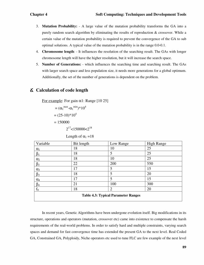
3. Mutation Probability: - A large value of the mutation probability transforms the GA into a

purely random search algorithm by eliminating the results of reproduction & crossover. While a

certain value of the mutation probability is required to prevent the convergence of the GA to sub

optimal solutions. A typical value of the mutation probability is in the range 0.0-0.1.

4. Chromosome length: - It influences the resolution of the searching result. The GAs with longer

chromosome length will have the higher resolution, but it will increase the search space.

5. Number of Generations: - which influences the searching time and searching result. The GAs

with larger search space and less population size, it needs more generations for a global optimum.

Additionally, the set of the number of generations is dependent on the problem.

�� Calculation of code length

For example: For gain α1: Range [10 25]

= (α1max-α1

min)*104

= (25-10)*104

= 150000

217<150000<218

Length of α1 =18

Variable Bit length Low Range High Range α1 18 10 25 β1 18 5 25 α2 18 10 25 β2 22 200 550 α3 17 5 15 β3 18 5 20 α4 17 5 15 β4 21 100 300 f0 18 2 20

Table 4.3: Typical Parameter Ranges

In recent years, Genetic Algorithms have been undergone evolution itself. Big modifications in its

structure, operations and operators (mutation, crossover etc) came into existence to compensate the harsh

requirements of the real-world problems. In order to satisfy hard and multiple constraints, varying search

spaces and demand for fast convergence time has extended the present GA to the next level. Real Coded

GA, Constrained GA, Polyploidy, Niche operators etc used to tune FLC are few example of the next level


90

GA [18 ,19]. Other new possibilities are also emerging by hybridization of other classical & evolutionary

methods with GA, for example amalgamation of Fuzzy Logic, Neural Networks, Particle Swarm,

Simulated Annealing with GA are used to tune the FLC for robot navigations.

In addition to choice of population strategy and all other GA parameters previously outlined, the

form of objective function used in evaluating GA-population members is an essential factor of the

optimization task [20]. In the realm of FLC optimization, numerous objective functions have been

adopted based on minimizing particular attributes of the system response such as the Mean Square Error

(MSE) [21], cost equations based on response rise and settling times and integral of absolute error (IAE)

[22]. Irrespective of definition, the suitability of the objective function as a system performance indicator

is critical to the successful application of a Genetic Algorithm and thus requires careful selection. Once

constructed around a suitable objective function, the GA proceeds to evaluate candidate solutions using

the objective function in order to gauge the performance of each potential solution when applied to the

problem domain [23]. Successful, and partially successful, solutions are rewarded by having “their

genetic information” perpetuated to successive generations in the search for the optimal solution, while

those potential solutions exhibiting poor performance are removed from “the genepool.”

4.6 Adaptive Neuro Fuzzy Inference System (ANFIS)

We can bring the low level learning & computational power of Neural Networks into

fuzzy systems and also high level humanlike IF- THEN rule thinking and reasoning of Fuzzy

system into neural networks ANFIS is a multi layer Neural Networks[24].

The acronym ANFIS derives its name from adaptive Neuro-fuzzy inference system. Using a given

input/output data set, the toolbox function ANFIS constructs a fuzzy inference system (FIS) whose

membership function parameters are tuned (adjusted) using either a backpropagation algorithm alone, or

in combination with a least squares type of method. This allows your fuzzy systems to learn from the data

they are modeling.

The basic idea behind these Neuro-adaptive learning techniques is very simple. These

techniques provide a method for the fuzzy modeling procedure to learn information about a data

set, in order to compute the membership function parameters that best allow the associated fuzzy

inference system to track the given input/output data. This learning method works similarly to

that of neural networks. Figure 4.4 shows the ANFIS architecture. The Fuzzy Logic Toolbox

function that accomplishes this membership function parameter adjustment is called ANFIS. The

ANFIS function can be accessed either from the command line, or through the ANFIS Editor


91

GUI. Since the functionality of the command line function ANFIS and the ANFIS Editor GUI is

similar.

Figure 4.4: ANFIS Architecture

There are FIVE layers in ANFIS MATLAB User Guide [25]:

Layer 1: Adaptive Layer [Premise]

Each node (i) is an adaptive node with a node function: O1,i = U Ai (x) for i = 1,2 O1,i = U B(i-2) (y) for i = 3,4 Where; x,y,… : Input to the node (i) Ai and B(i-2) : Linguistic Variables Parameters in this layer are called: Premise Parameters

Layer 2: Operator Layer [Fuzzy Operation]

This is a fixed node, whose output is product of all incoming signals. Each node represents firing strength of a rule (Any operator: min algebraic product, bounded product or drastic product ….. Can be used)

Layer 3: Normalizing Layer [Rule Strength]

The (i)th node calculates normalizes value of the weights using formulae


92

O3 = [ wi / (w1 + w2) ] for i=1,2... The output of the node is called Normalized strength.

Layer 4: Adaptive Layer [Consequence]

Each (i)th node is adaptive node with the function: O4= O3 *fi = O3 ( pi.x + qi.y + ri ) Where: O3 : Output of layer 3 ( pi., qi., ri ) : Consequent parameter set

Layer 5: Output Layer

The node computes overall output as sum of all incoming signals: O5,I = Σi [ O3,1* * fi ] = Σi O3,I / Σi wi

4.7 Software Development Tools The developments tools such as MATLAB, SIMULINK, and tools boxes are described in the

section. Their use is illustrated by applications.

4.7.1 MATLAB 7 MATLAB [26] is a high-performance language for technical computing. The name MATLAB

stands for MATrix LABoratory. A numerical analyst called Cleve Moler wrote the first version of

MATLAB in the 1970s. It has since evolved into a successful commercial software package. The

MATLAB system consists of five main parts:

�� Development Environment: -

This is the set of tools and facilities that help to use MATLAB functions and files. Many of these

tools are graphical user interfaces. It includes the MATLAB desktop and Command Window, a command

history, an editor and debugger, and browsers for viewing help, the workspace, files, and the search path.

The main features available in MATLAB are shown in Figure 4.5(a) and Main window of

MATLAB is as shown in Figure 4.5 (b).


93

Figure 4.5(a): a schematic diagram of Main features: MATLAB


94

Figure 4.5(b): MATLAB command window

The MATLAB Mathematical Function Library: - This is a vast collection of

computational algorithms ranging from elementary functions, like sum, sine, cosine, and

complex arithmetic.

The MATLAB Language: - This is a high-level matrix/array language with control flow

statements, functions, data structures, input/output, and object-oriented programming features.

The MATLAB Application Program Interface (API): - This is a library that allows

you to write C and FORTRAN programs that interact with MATLAB. It includes facilities for

calling routines from MATLAB (dynamic linking), calling MATLAB as a computational engine,

and for reading and writing MAT-files. Toolboxes available in MATLAB 7.0 and used in the

thesis are listed in Table 4.4.

Control System Toolbox Model Predictive Control Toolbox

Optimization Toolbox Robust Control

Neural Network Fuzzy Logic

Table 4.4: TOOL BOXES used from MATLAB 7


95

4.7.2 SIMULINK 6 Simulink [27] is a software package for modeling, simulating, and analyzing dynamic

systems. It supports linear and nonlinear systems, modeled in continuous time, sampled time, or

a hybrid of the two. Systems can also be multi rate, i.e., have different parts that are sampled or

updated at different rates. SIMULINK window is shown in Figure 4.6.

Figure 4.6: SIMULINK library browser window

Block set used from the SIMULINK 6.0 library are listed in Table 4.5.

Simulink Simulink Fixed Point

Simulink Accelerator Neural Network Block Set

Simulink Performance Tools Fuzzy Logic Block set

Simulink Response Optimization Fixed-Point Blockset

Table 4.5: Block sets used from SIMULINK 6

4.7.3 FUZZY Logic toolbox It is a collection of functions built on MATLAB. It provides tools to create and edit Fuzzy

Inference System. Fuzzy system can interact to SIMULINK model. Functions used to create fuzzy system

and their descriptions are given in Table 4.6 [28].


96

Functions description Addmf Add a membership function to an FIS Addrule Add a rule to an FIS Addvar Add a variable to an FIS Evalfis Perform fuzzy inference calculations Newfis Create new FIS Trimf Triangular membership function

Table 4.6: functions used to create fuzzy system

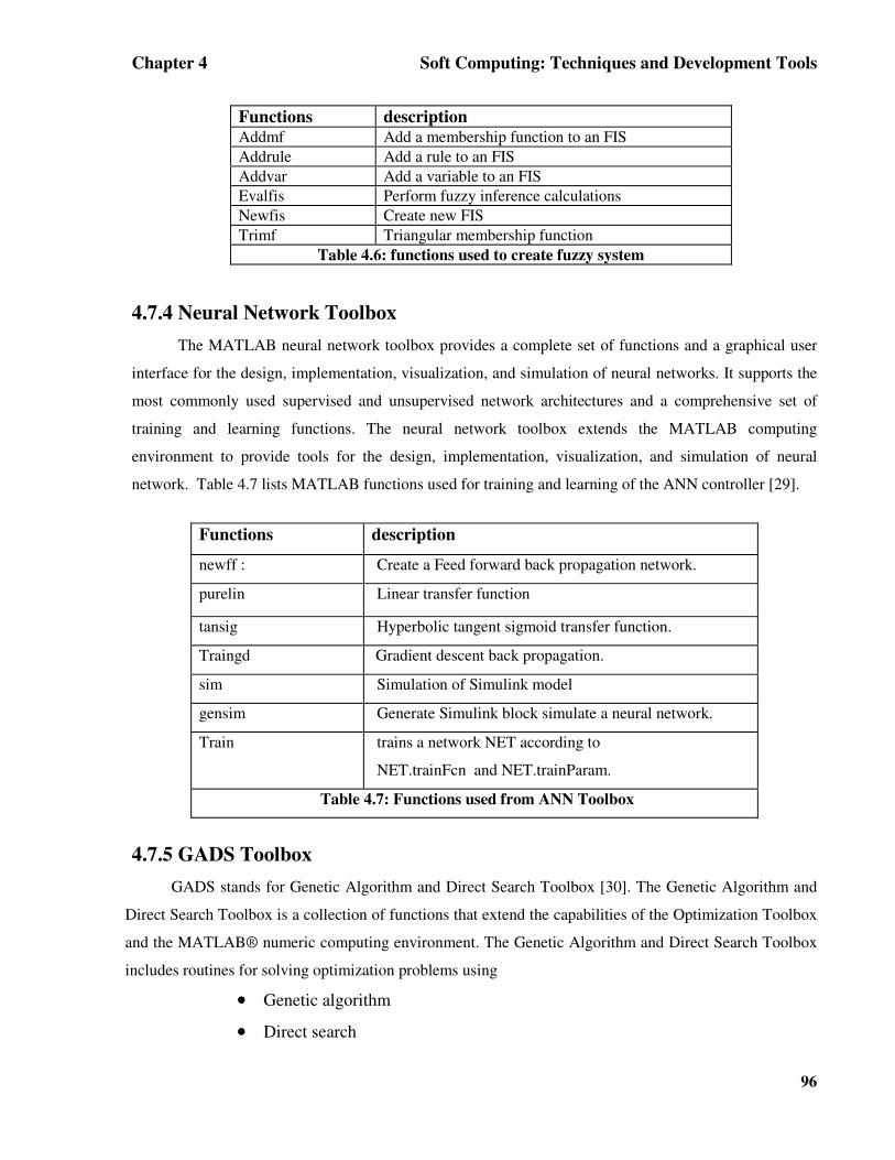
4.7.4 Neural Network Toolbox The MATLAB neural network toolbox provides a complete set of functions and a graphical user

interface for the design, implementation, visualization, and simulation of neural networks. It supports the

most commonly used supervised and unsupervised network architectures and a comprehensive set of

training and learning functions. The neural network toolbox extends the MATLAB computing

environment to provide tools for the design, implementation, visualization, and simulation of neural

network. Table 4.7 lists MATLAB functions used for training and learning of the ANN controller [29].

Functions description

newff : Create a Feed forward back propagation network.

purelin Linear transfer function

tansig Hyperbolic tangent sigmoid transfer function.

Traingd Gradient descent back propagation.

sim Simulation of Simulink model

gensim Generate Simulink block simulate a neural network.

Train trains a network NET according to

NET.trainFcn and NET.trainParam.

Table 4.7: Functions used from ANN Toolbox

4.7.5 GADS Toolbox GADS stands for Genetic Algorithm and Direct Search Toolbox [30]. The Genetic Algorithm and

Direct Search Toolbox is a collection of functions that extend the capabilities of the Optimization Toolbox

and the MATLAB® numeric computing environment. The Genetic Algorithm and Direct Search Toolbox

includes routines for solving optimization problems using

•••• Genetic algorithm

•••• Direct search


97

These algorithms enable you to solve a variety of optimization problems that lie outside

the scope of the standard Optimization Toolbox.

There are main four functions related to Genetic Algorithms available to the user in

Genetic Algorithm and Direct Search Toolbox as tabulated in Table 4.8.

ga Find the minimum of a function using the genetic algorithm

gaoptimget Get values of a genetic algorithm options structure

gaoptimset Create a genetic algorithm options structure

gatool Open the Genetic Algorithm Tool

Table 4.8:Function Description

4.7.6 ANFIS Editor To start ANFIS editor [26] GUI, on the MATLAB command prompt type the following….

>>anfisedit

Figure 4.7: ANFIS Editor GUI

The ANFIS Editor GUI is shown in Figure 4.7. The main functions in the anfisedit are

the loading of the training data from the work space. Then after by loading the training data into

the anfiseditor select the sub clustering button to generate the FIS model. After doing these steps


98

now select the training algorithm and error tolerance and number of epochs. Now press the train

button which will train the Neuro-fuzzy controller and it generates the training rules itself.

�� GENERAL DESIGN METHODOLOGY

1. Analyze the problem and find whether it has sufficient elements for a neural network solution.

Consider alternative approaches. A simple DSP/ASIC based direct solution may be satisfactory.

2. If the ANN is to represent a static function, then a three-layer feedforward network should be

sufficient. For a dynamic function select either a recurrent network or a time delayed network.

Information about the structure and order of the dynamic system is required.

3. Select input nodes equal to the number of input signals and output nodes equal to the number of

output signals and a bias source. For a feedforward network, select the initially hidden layer

neurons typically mean of input and output nodes.

4. Create an input/output training data table. Capture the data from an experimental plant or

simulation results, if possible.

5. Select input scale factor to normalize the input signals and the corresponding output scale factor

for denormalization.

6. Select generally a sigmoidal transfer function for unipolar output and a hyperbolic tan function for

bipolar output.

7. Select a development system, such an s Neural Network Toolbox in MATLAB.

8. Select appropriate learning coefficients (η) and momentum factor (µ).

9. Select an acceptable training error ξ and a number of epochs. The training will stop whichever

criterion was met earlier.

10. After the training is complete with all the patterns, test the network performance with some

intermediate data points.

11. Finally, download the weights and implement the network by hardware or software.

Summary The theoretical background of soft computing techniques such as fuzzy logic, ANN, GA and

ANFIS is summarized and described. Toolboxes available for deploying soft computing techniques in

MATLAB and used in our research work for the design and testing of proposed techniques are described

in detail. Procedural steps to be followed in each traits are discussed in detail.

Documents

shodhganga.inflibnet.ac.inshodhganga.inflibnet.ac.in/bitstream/10603/7499/14/14_chapter 4.pdf · C or ec t md lf ps a ynbv ix w h unacceptable assumptions. The classical modeling