4D Printing as a New Paradigm for Advanced Manufacturing

4D Printing as a New Paradigm for Advanced Manufacturing

by

Farhang Momeni

A dissertation submitted in partial fulfillment of the requirements for the degree of

Doctor of Philosophy (Mechanical Engineering)

in The University of Michigan 2018

Doctoral Committee:

Professor Jun Ni, Chair Associate Professor Kira Barton Professor Jinsang Kim Professor Jyoti Mazumder

Farhang Momeni

[email protected]

ORCID iD: 0000-0001-9596-3026

© Farhang Momeni 2018

All Rights Reserved

ii

ACKNOWLEDGEMENTS

I would like to thank:

• My parents.

• My advisor Prof. Jun Ni for his advice and support during this scientific journey.

• My committee members Prof. Jyoti Mazumder, Prof. Jinsang Kim, and Prof. Kira

Barton for their valuable comments and encouragements.

• My co-authors in the article related to chapter 1: Prof. Xun Liu that reviewed the

manuscript and provided feedback and Dr. Seyed M. Mehdi Hassani that helped me

in drawing some of the figures and checking the figure and citation numbering in the

related article.

• My co-authors in the article related to chapter 4: Reza Valizadeh; that I conceived the

related study with his input; Seyedali Sabzpoushan for CFD analysis; Seyedali

Sabzpoushan, Prof. Mohammad Reza Morad, and Reza Valizadeh for performance

analysis and useful discussions on other parts of the article related to this chapter, and

Prof. Xun Liu for useful discussions on various elements of the article related to this

chapter.

• The Mechanical Engineering Department at the University of Michigan for preparing

full funding for the whole duration of my direct Ph.D. program.

• S.M. Wu Manufacturing Research Center in the Mechanical Engineering Department

at the University of Michigan.

• Prof. Albert Shih for permission to use the printers in the S.M. Wu Manufacturing

Research Center.

• The Mechanical Engineering Department at the University of Michigan for use of the

Wind Tunnel facility in Lab I (ME 395), for which I served as a GSI (Graduate

iii

Student Instructor); Mr. Todd Wilber and Mr. John Laidlaw for assistance in setup

and usage.

• Mr. Andrea Poli for assistance in DMA tests in the Mechanical Testing Core directed

by Prof. Ellen Arruda in the ME Department at the University of Michigan.

• The course “Heat Transfer (ME 335)” taught by Prof. Massoud Kaviany at the

University of Michigan, for which I served as a GSI (Graduate Student Instructor).

• The courses “Assembly Modeling for Design and Manufacturing (ME 588)” and

“Design for Manufacturability (ME 452)” taught by Prof. Kazuhiro Saitou at the

University of Michigan, for which I served as a GSI (Graduate Student Instructor).

• The unlimited meal plan of the University of Michigan that saved my time.

• The Blue buses of the University of Michigan that even work after 11 PM and are

free.

iv

TABLE OF CONTENTS

ACKNOWLEDGEMENTS ................................................................................................... ii

LIST OF TABLES................................................................................................................ vi

LIST OF FIGURES ............................................................................................................. vii

ABSTRACT........................................................................................................................ xiv

CHAPTER 1 INTRODUCTION AND A REVIEW OF 4D PRINTING .............................. 1

1.1 Introduction........................................................................................................... 1 1.1.1 Definition........................................................................................................ 2 1.1.2 Motivations ..................................................................................................... 5

1.1.3 Various shape-shifting types and dimensions .................................................... 7 1.2 Material structures ................................................................................................. 7

1.2.1 Multi-material structures.................................................................................. 8 1.2.2 Digital materials .............................................................................................. 8

1.3 Materials ..............................................................................................................12 1.4 Shape-shifting mechanisms and Stimuli.................................................................17 1.5 Mathematics .........................................................................................................26 1.6 Conclusions..........................................................................................................33

1.7 Problem statement and dissertation structure ..........................................................33

CHAPTER 2 LAWS OF SHAPE-SHIFTING IN 4D PRINTING....................................... 35

2.1 Introduction..........................................................................................................36 2.2 Definitions, derivations, and discussions................................................................37

2.2.1 First law.........................................................................................................38 2.2.2 Second law.....................................................................................................38 2.2.3 Third law .......................................................................................................43

2.3 Conclusions..........................................................................................................62

CHAPTER 3 4D PRINTING AS A NEW PARADIGM FOR MANUFACTURING WITH

MINIMUM ENERGY CONSUMPTION............................................................................ 64

3.1 Introduction..........................................................................................................64 3.2 4D printing as a new manufacturing process with unique attributes ........................65

3.3 Energy aspect of 4D printing as a new process for self-assembly at manufacturing scale ...................................................................................................................................69

3.4 Conclusions..........................................................................................................72

v

CHAPTER 4 PLANT LEAF-MIMETIC SMART WIND TURBINE BLADES BY 4D

PRINTING .......................................................................................................................... 74

4.1 Introduction..........................................................................................................75 4.1.1 Adaptive wind turbine blades..........................................................................75 4.1.2 Bend-twist coupling in wind turbine blades .....................................................77

4.1.3 Flexible wind turbine blades ...........................................................................77 4.1.4 Plant leaf-mimetic wind turbine blades............................................................79

4.2 Mathematical modeling of the proposed blade .......................................................81 4.3 Fabrications and shape-shifting demonstrations .....................................................92

4.3.1 Results and discussions...................................................................................93 4.4 Wind tunnel tests ..................................................................................................98

4.4.1 Results and discussions...................................................................................99 4.5 CFD simulations and performance analysis ......................................................... 107

4.6 Dynamic Mechanical Analysis (DMA) tests ........................................................ 119 4.7 Discussions ........................................................................................................ 121

4.7.1 Mechanisms for applying stimulus ................................................................ 121 4.7.2 Small-scale and large-scale applications ........................................................ 122

4.7.3 Materials considerations ............................................................................... 123 4.7.4 Other plant-mimetic approaches useful for wind turbines ............................... 123

4.8 Conclusions........................................................................................................ 124

CHAPTER 5 NATURE-INSPIRED SMART SOLAR CONCENTRATORS BY 4D

PRINTING ........................................................................................................................ 125

5.1 Introduction........................................................................................................ 126 5.2 Design concept ................................................................................................... 127 5.3 Simulation .......................................................................................................... 130

5.4 Experiment ......................................................................................................... 139 5.5 Conclusions........................................................................................................ 143

CHAPTER 6 CONCLUSIONS AND FUTURE WORKS ................................................. 145

6.1 Conclusions........................................................................................................ 145

6.2 Future works ...................................................................................................... 146

APPENDIX A .................................................................................................................... 148

BIBLIOGRAPHY.............................................................................................................. 175

vi

LIST OF TABLES

Table 4-1. Designed veins dimensions and the angle between the main and lateral veins for

printing. ...............................................................................................................86

Table 4-2. Dimensions of PLA/paper composite in the blade structure demonstrated in

Figure 4-12. ..........................................................................................................87 Table 4-3. Values of parameters of our biexponential formula for a bilayer of PLA/paper

composite. Number 1 indicates the passive layer (paper) and number 2 indicates

the active layer (PLA). .........................................................................................90

Table 4-4. Values of parameters for calculating 𝐂𝐃, 𝐂𝐋 and 𝐑𝐞. ....................................... 105

vii

LIST OF FIGURES Figure 1-1. A simple illustration of the concept of 4D printing (Young, 2016)...................... 2 Figure 1-2. The differences between 3D printing and 4D printing processes. ....................... 3

Figure 1-3. 4D printing bases................................................................................................. 4 Figure 1-4. Stimulus-responsive materials (Sun et al., 2012). ................................................ 5 Figure 1-5. Shape-shifting types and dimensions in 4D printing. .......................................... 7 Figure 1-6. 4D-printed material structures (Digital Materials) (a) Uniform distribution with

different concentrations, (b) Gradient distribution, and (c) Special patterns. ..... 9 Figure 1-7. The simulation related to gradient distribution of material structure (red

indicates the passive material and purple indicates the active material) and the

results of its immersion in water over time (left to right) (Tibbits et al., 2014). ..10

Figure 1-8. Multi-material structures that have been used in 4D printing...........................10 Figure 1-9. Multi-material additive manufacturing system (Ge et al., 2016). ......................11 Figure 1-10. Illustration of structures with a smart hinge (Ge et al. 2014)...........................12 Figure 1-11. Structures with hinges vs. structures without hinges in 4D printing. ..............12

Figure 1-12. 4D printing materials. ......................................................................................17 Figure 1-13. Schematic illustration of the unconstrained-hydro-mechanics mechanism in 4D

printing. The green parts represent expandable materials. ................................18 Figure 1-14. Constrained-thermo-mechanics mechanism in 4D printing.............................20

Figure 1-15. Unconstrained-thermo-mechanics mechanism in 4D printing. ........................21 Figure 1-16. Unconstrained-hydro-thermo-mechanics mechanism in 4D printing. .............22 Figure 1-17. Unconstrained-pH-mechanics mechanism in 4D printing. ..............................23 Figure 1-18. Illustration of the unconstrained-thermo-photo-mechanics mechanism..........24

Figure 1-19 (a) Osmosis effect between two droplets, (b) Macroscopic deformation arising

from osmosis effect (Villar et al. 2013). ...............................................................25 Figure 1-20. Shape-shifting mechanisms and stimuli which were used in 4D printing. .......26 Figure 1-21. Repeated tests to identify the appropriate material structure to reach the precise

desired shape (Tibbits et al., 2014). .....................................................................27 Figure 1-22. Mathematical modeling of the 4D-printed hinge that was introduced earlier by

Tibbits et al. (2014) with the spring-mass concept (Raviv al. 2014).....................28 Figure 1-23. Standard linear solid (SLS) model to explain the mechanism of the shape

memory effect in a shape memory polymer (Yu et al. 2012). ..............................28 Figure 1-24. Four-element modeling of shape memory effect (Tobushi et al. 1997).............28 Figure 1-25. 4D printing mathematics allows theoretical models to connect the final desired

shape, material structure (or equivalently the size, shape and spatial arrangement

of the voxels or equivalently print paths and nozzle sizes), material properties, and

stimulus properties. .............................................................................................30 Figure 1-26. Mathematical modeling can make a connection between (a) print paths

quantified by the angle 𝜽 between the two layers, and (b) final desired shape

viii

quantified by curvature tensor 𝜿 , mean curvature 𝑯 , and Gaussian

curvature 𝑲(Gladman et al., 2016). .....................................................................31

Figure 1-27. Longitudinal and transverse swelling strains (𝜶 ∥ and 𝜶 ⊥) (Gladman et al.,

2016). ...................................................................................................................31 Figure 1-28. Print paths and final shapes (a) positive Gaussian curvature (b) negative

Gaussian curvature (c) and varying Gaussian curvature (Gladman et al., 2016).

.............................................................................................................................32 Figure 1-29. Using the concepts of the mean curvature, 𝑯, and Gaussian curvature, 𝑲 ,

generates the print paths by knowing the final desired morphologies (Gladman et

al., 2016)...............................................................................................................32 Figure 2-1. Toward the laws of shape-shifting in 4D printing. .............................................37 Figure 2-2. Toward the third law by analyzing the most fundamental multi-material 4D

structure. .............................................................................................................44

Figure 2-3. The general graph that exhibits the time-dependent behavior of almost all the

multi-material 4D printed structures (photochemical-, photothermal-, solvent-,

pH-, moisture-, electrochemical-, electrothermal-, ultrasound-, enzyme-, hydro-,

etc.-responsive). ...................................................................................................49

Figure 2-4. Analysis of the proposed model by experimental data from separate studies in

the literature (Le Duigou et al., 2016; Alipour et al., 2016; Nath et al., 2014; Zhou

et al., 2016; Li et al., 2015; Zhang et al., 2016), for both the on and off regions and

various stimuli such as moisture (Le Duigou et al., 2016), solvent (Alipour et al.,

2016), photochemical (Nath et al., 2014), photothermal (Zhou et al., 2016),

ultrasound (Li et al., 2015), and heat (Zhang et al., 2016). ..................................51

Figure 2-5. Depending on the relative values of 𝒂𝟏, 𝒂𝟐, 𝑬𝟏, and 𝑬𝟐, the relationship between

curvature and layers thicknesses would be different (it can be decreasing,

increasing, or a mixed behavior). This figure is based on equation (2-27). .........53 Figure 2-6. (a) The general effect of stimulus power (e.g., light intensity, pH value,

temperature magnitude, and so on) on time -dependent behavior. This plot is

based on equation (2-30). (b) Tuning the response speed, without changing the

final shape. This plot is based on equation (2-31). ...............................................56 Figure 2-7. A 4D structure with more than two types of materials. .....................................57 Figure 2-8. The simplified version of Figure 3-1, illustrating 4D printing process...............60

Figure 2-9. A summary of our laws. (the galactic shape of this figure has been inspired by a

display designed by Rod Hill, showing advancements in Reconfigurable

Manufacturing Systems, and installed on the wall of the ERC-RMS Center at the

University of Michigan.) ......................................................................................62

Figure 3-1. 4D printing process. ...........................................................................................67 Figure 3-2. “3S of 4D printing applications” and 4D printing attributes. ............................68 Figure 3-3. Future 4D printers. To achieve a 4D printer, an “intelligent head” (i.e., an

integrated software/hardware that incorporate s inverse mathematical problems

of Figure 3-1) should be developed and added to the current multi-material 3D

printers. ...............................................................................................................69 Figure 3-4. A manufacturing process in the most general thermodynamic model (this figure

has been drawn based on the concepts in (Gyftopoulos & Beretta, 2005; Gutowski

et al., 2006; 2007; 2009; Branham et al., 2008). The energy and entropy flows have

also been illustrated. ............................................................................................72

ix

Figure 4-1. Adaptability in wind turbine blades. (a) Bend-twist coupling adaptability (Hayat

et al., 2016) and (b) Sweeping adaptability (Sandia lab presentations, 2012)......76 Figure 4-2. Pre-bending deformation in flexible wind turbine blades to ensure tower

clearance (Bazilevs et al., 2012). ..........................................................................79 Figure 4-3. Pitch-angle change in flexible wind turbine blades. (a) airfoil with variable

camber (Hoogedoorn et al., 2010). (b) airfoil with constant fixed camber (Cognet

et al., 2017). ..........................................................................................................79

Figure 4-4. The simulations such as geometry optimizations performed by Liu et al. (2006;

2009; 2010; 2011) , demonstrated that wind blades based on the plant leaf

structure had better mechanical and structural properties such as the stiffness,

static strength, and fatigue life compared to the conventional structures (Liu et al.,

2006; 2009; 2010; 2011). ......................................................................................80 Figure 4-5. Various shape-shifting behaviors in wind turbine blades, and their advantages.

.............................................................................................................................81

Figure 4-6. Schematic illustrations of the desired bend-twist coupling in the proposed 4D

printed wind turbine blade based on the leaf structure: (a) Original flat blade, (b)

Desired deformed blade, and (c) bend angle (β) and twist angle (α) in the deformed

blade. ...................................................................................................................82

Figure 4-7. Illustration of the veins dimensions and the angle between the main and lateral

veins. ....................................................................................................................84 Figure 4-8. The behavior of the loss modulus of the PLA from DMA test (with the same

conditions considered for storage modulus in Figure 4-31). ................................90

Figure 4-9. The generated behavior of our biexponential formula for one strip and the real

behavior for multiple strips from Zhang et al. (2016). The exact number of strips

was not given in that experimental study (Zhang et al., 2016).............................91 Figure 4-10. Any deviation from the generated parameters in the step-by-step example,

cannot give the correct behavior. The experimental data are from Zhang et al.

(2016). ..................................................................................................................92 Figure 4-11. Printer TAZ 5 test setup for printing the plant-leaf mimetic architectures. ....93 Figure 4-12. (a) Originally printed flat blade without heat treatment (b) Bend-twist coupling

after heat treatment. ............................................................................................94 Figure 4-13. The technical advantages of the proposed wind turbine blade. .......................96 Figure 4-14. From purely rigid ancient wind turbines (such as Persian panemone (Dodge,

2006)) toward the future plant leaf-mimetic, smart, and eco-friendly wind

turbines. ...............................................................................................................97 Figure 4-15. Wind tunnel test setup......................................................................................99 Figure 4-16. (a) Drag load cell calibration, only for one horizontal direction. (b) Lift load cell

calibration, for both upward and downward vertical directions....................... 101

Figure 4-17. (a) Wind tunnel test on the samples installed on the sting, (b) flat sample

attached to the sting, (c) deformed sample connected to the sting and (d) wind

tunnel test on the pure sting. ............................................................................. 103 Figure 4-18. (a) Comparison of the lift force for the flat and deformed blades. (b) Comparison

of the drag force for the flat and deformed blades. ........................................... 104 Figure 4-19. (a) Comparison of the lift coefficient for the flat and deformed blades. (b)

Comparison of the drag coefficient for the flat and deformed blades. .............. 106 Figure 4-20. The top, frontal and lateral projections of the deflected 4D-printed blade.... 108

x

Figure 4-21. Comparison of lift force on a fixed deformed blade as a function of wind speed

between results of the wind tunnel tests and CFD simulations.......................... 109 Figure 4-22. Comparison of drag force on a fixed deformed blade as a function of wind speed

between results of the wind tunnel tests and CFD simulations.......................... 109 Figure 4-23. The increment of deformed blade RPM as the wind blows in higher speeds. 110 Figure 4-24. Generated lift on deflected shape of the proposed 4D-printed blade and its flat

shape at different wind speeds. .......................................................................... 111

Figure 4-25. The sliced-periodic domain used for simulation of a rotor disk with 6 blades,

containing only a couple of those blades. ........................................................... 112 Figure 4-26. Variation of generated torque per blade as a function of the total number of

blades in a full rotor disk (at the wind speed of 9.4 m/s). .................................. 113

Figure 4-27. Performance curve of the 6-bladed rotor disk power coefficient vs. tip speed

ratio in five different wind speeds...................................................................... 115 Figure 4-28. Velocity contours in 4 different chord-wise cross sections along the blade span

(0.01, 0.3, 0.6 and 0.9 of span). ........................................................................... 116

Figure 4-29. Air streamlines passing around the stationary 4D-printed blade in four different

chord-wise cross sections along the blade span. (a) 0.01, (b) 0.3, (c) 0.6 and (d) 0.9

of span................................................................................................................ 117 Figure 4-30. Static pressure (gauge) contours in 4 different chord-wise cross sections along

the blade span. (a) 0.01, (b) 0.3, (c) 0.6 and (d) 0.9 of span. ............................... 118 Figure 4-31. The behavior of the elastic (storage) modulus of the “treated printed” PLA from

DMA test............................................................................................................ 121 Figure 4-32. The behavior of the elastic (storage) modulus of the “molded” and “annealed”

PLA from DMA test (Cock et al., 2013)............................................................. 121 Figure 5-1. Comparing the configurations of petals in diurnal and nocturnal flowers.

Category (a) shows some popular nocturnal flowers. They are closed around noon

and are open far from noon. Category (b) illustrates some popular diurnal flowers.

They are open around noon and are closed far from noon (Palermo, 2013; Villazon,

2009; Taylor, 2017; Wikipedia. Mirabilis jalapa, accessed 2017; Waluyo, 2015; Wikipedia. Nicotiana tabacum, accessed 2017; Taylor, 2017; Wooden Shoe Tulip

Farm, accessed 2017; Gardenia, accessed 2017). ............................................... 129

Figure 5-2. The specular reflection in flowers` petals. The flower photo of this figure was

taken by Dekker (accessed 2017). ...................................................................... 130 Figure 5-3. Concepts and procedures of Ray tracing simulations and optical analysis using

TracePro. ........................................................................................................... 132

Figure 5-4. Comparison of the optical efficiency in four well-known concentrators, i.e.,

elliptic, parabolic, V-shape, and hyperbolic. All the four concentrators have equal

heights and concentration ratios (H=10 mm and CR=2.35). (a) shows CAD

(Computer-Aided Design) models of the four concentrators that were simulated

in ray tracing software. (b) exhibits the optical efficiency of the four shapes

illustrated in part (a), over various irradiation angles. ..................................... 133 Figure 5-5. Overall optical efficiency in three different cases. ........................................... 134 Figure 5-6. The effect of concentrator`s height on the optical efficiency of CHC at various

solar irradiance angles. H= 10 mm is the reference value that was used in Figure

5-4. The concentration ratio and head configuration are kept constant at all

xi

various heights. This result indicates that higher height usually leads to lower

optical efficiency at all incidence angles. ........................................................... 136 Figure 5-7. The reason of less optical efficiency in concentrators with higher heights by flux-

based ray color analysis. The concentration ratio and head configuration are the

same in both cases.............................................................................................. 137 Figure 5-8. The effect of concentration ratio (CR) on the optical efficiency of CHC at various

solar irradiance angles. The height is similar in all cases. This result indicates that

higher CR leads to lower optical efficiency at all incidence angles.................... 137 Figure 5-9. The effect of our so-called Trapping Zone on the optical efficiency of CHC at

various solar irradiance angles . The concentration ratio, height, and head

configuration are kept constant in both of the cases.......................................... 138

Figure 5-10. The effect of our so-called Entry Curvature on the optical efficiency of CHC at

various solar irradiance angles. The concentration ratio and height are kept

constant in both the cases. ................................................................................. 139 Figure 5-11. Design, manufacturing, and desired shape -shifting. (a) illustrates the design

process. (b) exhibits the fabrication steps that consis t of three processes. Process

1 shows one example of the PLA printing on a paper sheet. (c) shows the desired

reversible shape-shifting between hyperbola at low temperatures (consistent with

the weather conditions far from noon) and parabola at high temperatures

(consistent with the weather conditions around noon). Scale bars are 3.5 cm. . 141 Figure A-1. Illustration of the difference between one -way and two-way shape memory

materials (Hager et al., 2015)............................................................................. 149 Figure A-2. Illustration of dual and triple SME (Hager et al., 2015), where A is the permanent

shape. ................................................................................................................. 149 Figure A-3. The difference between folding and bending (Liu et al., 2016)........................ 150 Figure A-4. Surface topography: wrinkling, creasing, and buckling (Wang & Zhao, 2014).

........................................................................................................................... 150

Figure A-5. The illustration of 1D-to-1D shape-shifting by linear expansion/contraction

adapted from (Raviv et al., 2014)....................................................................... 151 Figure A-6. The illustration of 1D-to-1D shape-shifting by linear expansion/contraction

adapted from (Yu et al., 2015). .......................................................................... 151

Figure A-7. The illustration of 1D-to-2D shape-shifting by self-folding (Tibbits, 2014). .... 152 Figure A-8. An illustration of 1D-to-2D sinusoidal shape-shifting by self-bending (Tibbits et

al., 2014)............................................................................................................. 152 Figure A-9. The self-folding of 1D strand to 3D wireframe cube (Tibbits, 2014). .............. 153

Figure A-10. Two passive discs to tune the final folding angle (Tibbits, 2014)................... 153 Figure A-11. Shape-shifting from a 1D strand to a 3D structure of Crambin protein based

on self-folding (Tibbits et al., 2014). .................................................................. 153 Figure A-12. 2D-to-2D self-bending in which a rectangular network transforms into a circle.

Scale bar, 200 µ𝐦 (Villar et al., 2013)................................................................ 153 Figure A-13. Multi-shape memory effect from 2D to 3D by self-bending in a smart trestle

(Wu et al., 2016). ................................................................................................ 154 Figure A-14. Multi-shape memory effect from 2D to 3D by self-bending in an active helix

shape (Wu et al., 2016)....................................................................................... 154 Figure A-15. Multi-shape memory effect from 2D to 3D by self-bending in an active wave

shape (Wu et al., 2016)....................................................................................... 154

xii

Figure A-16. Multi-shape memory effect from 2D to 3D by self-bending in a smart insect-

like structure (Wu et al., 2016). ......................................................................... 155 Figure A-17. Multi-shape memory effect from 2D to 3D by self-bending in a smart hook (Wu

et al., 2016). ........................................................................................................ 155 Figure A-18. Flower-like 4D structure. (a) The original flat sheet. (b) The final flower-like

structure. (c) A complex structure created by tearing paper off the flower-like 3D

structure (Zhang et al. 2016). ............................................................................ 155

Figure A-19. A 3D periodic structure created from a 2D sheet by self-bending (Zhang et al.,

2016). ................................................................................................................. 156 Figure A-20. A bio-origami 2D pattern transforms into a 3D pattern by self-bending: (a)

Schematic illustration of the self-bending of PEG bilayer. (b) A fluorescent

micrograph of a self-bended bilayer (Jamal et al., 2013)................................... 156 Figure A-21. (a) The experiment related to 2D-to-3D self-bending in which a flower-shaped

network transforms into a hollow sphere. Scale bar, 200 µm (b) Simulation of (a)

(Villar et al., 2013). ............................................................................................ 157 Figure A-22. An illustration of 2D to 3D shape-shifting by self-folding to make a cube (Tibbits,

2014). ................................................................................................................. 157

Figure A-23. 2D-to-3D self-folding to make a truncated octahedron (Tibbits et al., 2014).

........................................................................................................................... 158 Figure A-24. An illustration of a 2D-to-3D alteration in which some origami shapes, such as

an origami box, pyramid, and airplane can be generated by self-folding (Ge et al.,

2014). ................................................................................................................. 158 Figure A-25. Sequential self-folding from 2D to 3D (Mao et al., 2015)............................... 159 Figure A-26. Helical structures with different degrees of spiral by 2D-to-3D twisting (Zhang

et al., 2016). ........................................................................................................ 159

Figure A-27. 2D-to-3D sinusoidal shape-shifting by surface curling (Tibbits et al., 2014). 160 Figure A-28. An illustration of 2D-to-3D hair-like shape-shifting by surface curling (Tibbits

et al., 2014). ........................................................................................................ 160 Figure A-29. 2D-to-3D surface curling (Raviv et al., 2014). ............................................... 160

Figure A-30. An illustration of 2D-to-3D alteration in which a complex, non-uniform

curvature sculpture is achieved: (a) Schematic of the flat laminate. (b) The final

desired shape after the thermo-mechanical experiment (Ge et al., 2013). ......... 161 Figure A-31. An illustration of 2D-to-3D surface topographical changes where mountains

and valleys are created on a flat surface (Tibbits et al., 2014). .......................... 161 Figure A-32. 2D-to-3D shape-shifting with surface topography (Tibbits et al., 2014). ....... 162 Figure A-33. 2D-to-3D shape-shifting by the combination of bending and twisting with

complex flower morphologies (Gladman et al., 2016)........................................ 162

Figure A-34. Various 2D-to-3D shape-shifting behaviors (Ge et al., 2013)......................... 163 Figure A-35. An illustration of 3D-to-3D self-bending in a bio-printed structure (Kokkinis et

al., 2015)............................................................................................................. 163 Figure A-36. 3D to 3D self-bending in a prosthetic finger (Mutlu et al., 2015)................... 164

Figure A-37. 3D-to-3D shape-shifting by expansion and contraction (Bakarich et al., 2015).

........................................................................................................................... 164 Figure A-38. Illustration of global and local shrinkage and bending for 3D-to-3D alterations

by using two different stimuli (Kuksenok et al., 2016). ..................................... 164

xiii

Figure A-39. Smart key–lock connectors that can be employed for various purposes

(Kokkinis et al., 2015). ....................................................................................... 166 Figure A-40. (a) Computer-aided design of the smart valve, (b) Printing of the valve, (c) 4D

printed valve in cold water, and (d) hot water (Bakarich et al., 2015). ............. 166 Figure A-41. pH-responsive flow regulating smart valve (Nadgorny et al., 2016).............. 167 Figure A-42. Thermo-responsive adaptive metamaterials with tunable bandgaps (Zhang et

al., 2016)............................................................................................................. 167

Figure A-43. Thermo-responsive adaptive metamaterials with tunable structures (Bodaghi

et al., 2016). ........................................................................................................ 168 Figure A-44. Elastomer metamaterials (Jiang & Wang, 2016)........................................... 168 Figure A-45. A 4D-printed, thermo-responsive stent which is able to reversibly change its

diameter and height (Ge et al., 2016). ................................................................ 170 Figure A-46. A 4D-printed, thermo-responsive stent which is able to reversibly change its

diameter (Bodaghi et al., 2016). ......................................................................... 170 Figure A-47. 4D printed thermo-responsive tracheal stent (Zarek et al., 2016). ................ 171

Figure A-48. 4D-printed shape memory gripper that can reversibly grab and release the

objects by heat (Ge et al., 2016). ........................................................................ 171 Figure A-49. Adaptability of textiles made of SMP vs. the textiles made of elastic fibers (Hu

et al., 2012). ........................................................................................................ 172

Figure A-50. Automated construction of a building in a single run using contour crafting

technology (Khoshnevis, 2004)........................................................................... 173 Figure A-51. Applications of the 4D printing process. ....................................................... 174

xiv

ABSTRACT

4D printing is a new manufacturing paradigm that combines stimuli-responsive materials,

mathematics, and multi-material additive manufacturing to yield encoded 3D structures with

intelligent behavior over time. This field has received growing interests from various disciplines

such as space exploration, renewable energy, bioengineering, textile industry, infrastructures, soft

robotics, etc. Here, after a review of 4D printing, three substantial gaps are identified. First, the

main difference between 3D and 4D printed structures is one extra dimension that is smart

evolution over “time”. However, currently, there is no general formula to model and predict this

extra dimension. This gap pertains to the design aspect of 4D printing. Second, 3D printing is a

well-known manufacturing process with its unique attributes. Now, 4D printing needs to be

underpinned as a manufacturing process and its unique attributes should also be proved. This gap

pertains to the manufacturing aspect of 4D printing. Third, various shape-morphing 4D printed

structures have been illustrated in the literature. However, real applications and products, where

4D printing can provide unique features still need to be demonstrated. This gap pertains to the

product development aspect of 4D printing.

To address the first gap (design), we delve into the fourth dimension and reveal three general

laws that govern the shape-shifting behaviors of almost all (photochemical-, photothermal-,

solvent-, pH-, moisture-, electrochemical-, electrothermal-, ultrasound-, etc.-responsive) multi-

material 4D structures. By starting from fundamental concepts, we derive and validate a universal

bi-exponential formula that is required to model and predict the fourth dimension of 4D multi-

materials. Our results, starting from the most fundamental concepts and ending with governing

equations, can serve as general design principles for future research in 4D printing, where the time -

dependent behaviors should be understood, modeled, and predicted correctly. Future 4D printing

software and hardware developments can also benefit from these results.

xv

To address the second gap (manufacturing), first, we underpin 4D printing as a new

manufacturing process and identify its unique attributes. Then, we specifically focus on the energy-

saving attribute of 4D printing. We obtain the theoretical limit of energy consumption in 4D

printing and prove that 4D printing can be the most energy-efficient manufacturing process.

To address the third gap (product development), we demonstrate two real applications, where

4D printed products can provide unique features. First, we demonstrate a novel wind turbine blade

based on 4D printing that provides several advantages in one blade, simultaneously. Scientists

reported that leaf veins grow in a manner not only to facilitate their biological and physiological

functions but also to sustain the environmental loads. Researchers showed that plant-leaf-mimet ic

blades could always have better structural properties compared with the conventional structures.

However, the plant-leaf-mimetic blade has remained at the level of simulations. We demonstrate

the plant-leaf-mimetic blade in practice that simultaneously has the capability of bend-twist-

coupling. Second, we introduce the concept of smart solar concentrators inspired by nature and

enabled by 4D printing. We found that diurnal flowers mainly have parabolic and nocturnal

flowers mainly have hyperbolic petals. Based on this inspiration, we propose a smart solar

concentrator that can increase the overall optical efficiency more than 25% compared with its non-

smart counterparts.

1

CHAPTER 1

INTRODUCTION AND A REVIEW OF 4D PRINTING

Research into 4D printing has attracted unprecedented interest since 2013 when the idea was

first introduced. It is based on 3D printing technology, but requires additional stimulus and

stimulus-responsive materials. Based on certain interaction mechanisms between the stimulus and

smart materials, as well as appropriate design of multi-material structures from mathematical

modeling, 4D printed structures evolve as a function of time and exhibit intelligent behavior. 4D

printing targets a time-dependent and predictable shape/property/functionality evolution. This

allows for self-assembly, self-adaptability, and self-repair. This chapter presents a comprehensive

review of the 4D printing process and summarizes the practical concepts and related tools that

have a prominent role in this field. Unsought aspects of 4D printing are also studied and organized

for future research.1

1.1 Introduction

3D printing was invented in the 1980s and has been applied in various fields, ranging from

biomedical science to space science. 4D printing, a recently developed field originating from 3D

printing, shows promising capabilities and broad potential applications. 4D printing was initiated

and termed by a research group at MIT (Tibbits, 2013). It relies on the fast growth of smart

materials, 3D printers, design (Choi et al., 2015), and mathematical modeling. 4D printing shows

advantages over 3D printing in several aspects (Jacobsen, 2016).

In this review, a general guideline is provided by deconstructing the 4D printing into several

sections. These sections include definition, motivations, shape-shifting behaviors, material

structures, materials, shape-shifting mechanisms and stimuli, mathematics, and applications.

1 This chapter is based on our journal article published in Materials & Design 122 (2017), entitled “A review of 4D

printing”, by Farhang Momeni, Seyed M.Mehdi Hassani, Xun Liu, and Jun Ni.

2

1.1.1 Definition

4D printing was initially defined as 4D printing = 3D printing + time (Figure 1-1), where the

shape, property, or functionality of a 3D printed structure can change as a function of time (Tibbits,

2013; 2014; Tibbits et al., 2014; Ge et al., 2013; Pei, 2014; Khoo et al., 2015). As the number of

studies conducted on this technology increases, a more comprehensive definition of 4D printing is

necessary and presented here. 4D printing is a targeted evolution of the 3D printed structure, in

terms of shape, property (other than shape), or functionality. It is capable of achieving self-

assembly, self-adaptability, and self-repair. It is time-dependent, printer-independent, and

predictable.

Figure 1-1. A simple illustration of the concept of 4D printing (Young, 2016).

As mentioned above, 4D printing can fabricate dynamic structures with adjustable shapes,

properties, or functionality (Tibbits et al., 2014; Pei, 2014; Gladman et al., 2016). This capability

mainly relies on an appropriate combination of smart materials in the three-dimensional space

(Gladman et al., 2016). Mathematical modeling is required for the design of the distribution of

multiple materials in the printed structure. There are at least two stable states in a 4D printed

structure, and the structure can shift from one state to another under the corresponding stimulus

(Zhou et al., 2015). The differences between 3D printing and 4D printing processes are illustrated

in Figure 1-2.

3

Figure 1-2. The differences between 3D printing and 4D printing processes.

As illustrated in Figure 1-3, the fundamental building blocks of 4D printing are 3D printing

facility, stimulus, stimulus-responsive material, interaction mechanism, and mathematical

modeling. These elements enable targeted and predictable evolution of 4D printed structures over

time and are discussed in further detail below:

⚫ 3D printing facility: Usually, a 4D printed structure is created by combining several materials

in the appropriate distribution into a single, one-time printed structure (Raviv et al., 2014).

The differences in material properties, such as swelling ratio and thermal expansion

coefficient, will lead to the desired shape-shifting behavior. Therefore, 3D printing is

necessary for the fabrication of multi-material structures.

⚫ Stimulus: Stimulus is required to trigger the alterations of shape/property/functionality of a

4D printed structure. The selection of the stimuli depends on the requirements of the specific

application, which also determines the types of smart materials.

⚫ Smart or stimulus-responsive material: Stimulus-responsive material is one of the most critical

components of 4D printing. Stimulus-responsive materials can be classified into several sub-

categories, as shown in Figure 1-4. The capability of this group of materials is defined by the

following characteristics: self-sensing, decision making, responsiveness, shape memory, self-

adaptability, multi-functionality (Khoo et al., 2015), and self-repair. Several review studies on

MaterialsStatic

structure

Smart and

passive

materials

Static

smart

structure

Dynamic

smart

structure

3D

printing

4D

printing

3D printer

Mathematics:

Usually an inverse

problem

Stimulus

Multi-material

3D printer

Interaction

mechanism

4

stimulus-responsive materials have been provided by Roy et al. (2010), Stuart et al. (2010),

Sun et al. (2012), and Meng et al. (2013).

⚫ Interaction mechanism: In some cases, the desired shape of a 4D printed structure is not

directly achieved by simply exposing the smart materials to the stimulus. The stimulus needs

to be applied in a certain sequence under an appropriate amount of time, which is referred to

as the interaction mechanism in this review study. For example, one of the main interaction

mechanisms is constrained-thermo-mechanics. In this mechanism, the stimulus is heat and the

smart material has the shape memory effect. It contains a 4-step cycle. First, the structure is

deformed by an external load at a high temperature; second, the temperature is lowered while

the external load is maintained; third, the structure is unloaded at the low temperature and the

desired shape is achieved; fourth, the original shape can be recovered by reheating.

⚫ Mathematical modeling: Mathematics is necessary for 4D printing in order to design the

material distribution and structure needed to achieve the desired change in shape, property, or

functionality. Theoretical and numerical models need to be developed to establish the

connections between four core elements: material structure, desired shape, material properties,

and stimulus properties. These will be discussed in additional details later.

Figure 1-3. 4D printing bases.

3D Printing

FacilityStimulus

Smart (stimulus-

responsive) Material

4D Printing Bases

Interaction

Mechanism

Mathematical

Modeling

5

Figure 1-4. Stimulus-responsive materials (Sun et al., 2012).

A 4D printed structure can be regarded as a child born from the marriage between a 3D

printer and smart materials. It can walk by being exposed to the external stimulus through an

interaction mechanism, and it learns how to walk properly with the assistance of mathematics.

1.1.2 Motivations

4D printing opens new fields for application, in which a structure can be activated for self-

assembly, reconfiguration, and replication through environmental free energies (Tibbits, 2014).

This brings several advantages, such as significant volume reduction for storage, and

transformations that can be achieved with flat-pack 4D printed structures. The latter may include

transformations to 3D structures required during actual applications (Tibbits, 2014). Another

example is that instead of directly creating a complicated structure using the 3D printing process,

simple components from smart materials can be 3D printed first and then self-assembled to reach

6

that final complex shape (Zhou et al., 2015). In general, the applications of 4D printed structures

can be classified into three categories: self-assembly, self-adaptability, and self-repair.

• Self-assembly:

Self-assembly extends from the molecular scale to the planetary scale (Whitesides &

Grzybowski, 2002; Campbell et al., 2014). Currently, researchers are interested in macroscale

applications (Campbell et al., 2014). One example is the transfer of equipment parts to the inside

of a human body through a small hole. The parts can then self-assemble at the desired location for

medical purposes (Zhou et al., 2015). Another future application of self-assembly will be on a

large scale and in a harsh environment. Individual parts can be printed with small 3D printers and

then self-assembled into larger structures, such as space antennae and satellites (Tibbits et al.,

2014). This capability paves the way for the creation of transportation systems to the International

Space Station (Choi et al., 2015). Further applications include self-assembling buildings ,

especially in war zones or in outer space where the elements can come together to yield a finished

building with minimum human involvement (Campbell et al., 2014). Moreover, some limitations

in architectural research and experiments can be removed with the capabilities of 4D printing

(Čolić-Damjanovic & Gadjanski, 2016).

• Self-adaptability:

Adaptive infrastructures are another application of 4D printing (Campbell et al., 2014). 4D

printing can integrate sensing and actuation directly into a material so that external

electromechanical systems are not necessary (Tibbits et al., 2014). This would decrease the number

of parts in a structure, assembly time, material and energy costs, as well as the number of failure -

prone devices, which is usually utilized in current electromechanical systems (Tibbits et al. , 2014).

Multi-functional and self-adaptive 4D printed tissues (Khademhosseini & Langer, 2016; Jung et

al., 2016) and 4D-printed medical devices, such as tracheal stents (Zarek et al., 2017) and

cardiovascular devices (Robinson et al., 2018) are other fascinating applications of 4D printing.

• Self-repair:

The idea of self-assembly can be utilized for self-disassembly. The error-correct and self-

repairing capability of 4D manufactured products show tremendous advantages with regard to

reusability and recycling (Tibbits, 2014). Self-healing pipes (Campbell et al., 2014) and self-

healing hydrogels (Taylor, 2016) are some of the potential applications.

7

1.1.3 Various shape-shifting types and dimensions

Various shape-shifting types and dimensions that have been studied in 4D printing are

categorized in Figure 1-5 along with the related literature (details in Appendix A).

Figure 1-5. Shape-shifting types and dimensions in 4D printing.

In the following, we delve into the elements of 4D printing seen in Figure 1-2. The reader is

also invited to have a look at Appendix A for details of various shape-shifting behaviors and

applications of 4D printing.

1.2 Material structures

Details of material types are discussed in the next section. In this section, material structures

are classified and generally referred to as smart materials and conventional (non-smart) materials.

In additive manufacturing, material structures are divided into single-material and multi-materia l

structures. According to Vaezi et al. (2013), multi-material structures can be further classified into

• Ge et al. (2013)

•Jamal et al. (2013)

•Villar et al. (2013)

•Yu et al. (2015)

• Gladman et al. (2016)

• Wu et al. (2016)

•Zhang et al. (2016)

•Ge et al. (2016)

1D 3D 1D 2D

Shape Shifting Types and Dimensions

•Kuksenoket al. (2016)

Surface

Topography•Tibbits et al. (2014)

Surface

Curling

Nonlinear

shrinkage

Twisting

Folding

Folding

Bending

•Tibbits (2014)

•Raviv et al. (2014)

FoldingBending

• Mutlu et al. (2015)

• Kuksenoket al. (2016)

• Kokkinis et al. (2015)

• Yu et al. (2015)

• Ge et al. (2016)

Linear

shrinkage

•Ge et al. (2013)

•Gladman et al. (2016)

3D 3D

•Tibbits et al. (2014)


Bending

2D 2D 1D 1D

Linear

contraction/

expansion


•Yu et al. (2015)

•Villar et al. (2013)•Tibbits (2014)


•Ge et al. (2016)

2D 3D

Bending

Bending

and

Twisting


•Ge et al. (2013)


•Ge et al. (2013)



•Bakarich et al. (2015)

•Nadgorny et al. (2016)

•Tibbits (2014)




•Ge et al. (2014)

•Mao et al. (2015)

•Naficy et al. (2016)

8

discrete multiple materials, composite materials, and porous materials. For the 4D printing process,

a new classification is introduced in this review, and the multi-material structure can be categorized

as uniform distribution, gradient distribution, and special patterns. Based on different perspectives,

the material structure can also be classified as a structure with or without joints and hinges.

1.2.1 Multi-material structures

In 4D printing, multiple materials usually need to be inserted into a single and one-time

printed structure (Raviv et al., 2014). This multi-material structure can be a mixture of different

smart materials or a combination of smart materials and conventional materials. The single -

material structure in 4D printing should always be fabricated with a smart material. In addition, it

needs to be based on the structure with a gradient distribution of materials. The gradient

distribution of a single material means that the density of the structure is different at various

locations. This anisotropy can generate shape-shifting behaviors such as bending and twisting,

which is beyond linear expansion and contraction. Most of the previous studies on 4D printing

focused on multi-material structures. In this review, the concept of digital material is described for

4D printing. Based on this concept, all material structures involved in 4D printing can be

generalized into three categories.

1.2.2 Digital materials

The digital concept was first introduced in the fields of communication and computation.

This digital concept can be similarly expanded into material structures (Hiller et al., 2009). The

element that enables us to move from analog materials to digital materials is the physical voxel

(Hiller et al., 2009), which is defined as the fundamental and physical bit that occupies 3D physical

space. The physical voxel can be of any size and shape (Hiller & Lipson, 2009; 2010; Popescu et

al., 2006). In nature, biological structures usually consist of fundamental building blocks that can

be considered physical voxels, such as DNA and proteins (Hiller et al. 2009). In 4D printing and

associated multi-material structures, the physical voxel can be similarly defined.

Digital material is defined as an assembly of various physical voxels (Hiller & Lipson, 2009;

2010). The spatial arrangement of voxels plays a major role in determining the features of a 4D-

printed structure (Raviv et al., 2014). In digital materials, each voxel contains only one material.

Adjacent voxels can be composed of different materials. Each voxel has its own properties and the

collection of different voxels results in the multi-material structure. According to Hiller et al.

9

(2010), a negative Poisson’s ratio can be achieved with appropriate voxel arrangement in the

digital material structure.

The three most important categories of 4D-printed structures for digital materials are uniform

distribution (Figure 1-6 (a)), gradient distribution (Figure 1-6 (b)), and special patterns (Figure 1-6

(c)). One main category of special patterns is the fiber and matrix structure. Each structure in

Figure 1-6 shows only one single layer, but they can be combined to yield bi-layer or multi-layer

structures. In addition, the number of materials can be more than two. One example of a gradient

distribution material structure is shown in Figure 1-7 from Tibbits et al. (2014). In this example,

the concentration of active and passive materials varies from the center to the perimeter within one

layer. The disk can yield various sinusoidal shapes depending on the duration of immersion in

water.

Figure 1-6. 4D-printed material structures (Digital Materials) (a) Uniform distribution

with different concentrations, (b) Gradient distribution, and (c) Special patterns.

Multi-Material Structure in 4D printing

Uniform Distribution with Different Concentrations

Gradient Distribution

One Way Direction GradientFrom Center to Edge Gradient

Special Patterns

Voxel Type 1:

Voxel Type 2:a

b

c

10

Figure 1-7. The simulation related to gradient distribution of material structure (red

indicates the passive material and purple indicates the active material) and the results of its

immersion in water over time (left to right) (Tibbits et al., 2014).

In summary, all multi-material structures that have been studied in the 4D printing process

are summarized in the following figure, along with the related literature.

Figure 1-8. Multi-material structures that have been used in 4D printing.

To model the material structure in various length and time scales for digital materials, Myres

et al. (1999) developed a software called the Digital Material (Myers et al., 1998). Popescu et al.

(2006) proposed a new manufacturing process for digital materials that was reversible for

disassembly and could reuse the building blocks of the structure. Huang et al. (2016) demonstrated

an approach for ultrafast printing of shape-shifting materials. Zhou et al. (2013) reported that there

were several limitations to the current additive manufacturing processes. For example, printers

with inkjet nozzles could only print materials with certain viscosities and curing temperatures. The

fused deposition modeling (FDM) process was relatively slow and had limited options for its

minimum nozzle size. Zhou et al. (2013) investigated several new techniques for digital material

Uniform distribution with different concentrations Gradient distribution structure Special Patterns

Material structure in 4D printing

•Ge et al. (2013)

•Ge et al. (2014)

•Kuksenok et al. (2016)


•Wu et al. (2016)


•Duigou et al. (2016)

•Bodaghi et al. (2016)



•Kokkinis et al. (2015)



•Tibbits (2014)



•Mao et al. (2015)


•Zarek et al. (2016)


•Ge et al. (2016)

11

production using mask-image-projection-based stereolithography. Ge et al. (2016) provided an

approach for printing multi-material shape memory polymers (SMPs) with a high resolution (up

to a few microns). This approach is enabled by a high-resolution projection microstereolithography

(PμSL) additive manufacturing system with an automated material exchange mechanism (Figure

1-9). In order to enable 4D printing for biomedical applications, multi-material additive

manufacturing systems that can print from aqueous mediums needs to be developed (Loh, 2016) .

In this regard, the direct-write (DW) printing technique (Lewis, 2006; Gratson & Lewis, 2005;

Lebel et al., 2010), which is suitable for printing polymeric solutions (Guo et al., 2013), can be

engaged.

Figure 1-9. Multi-material additive manufacturing system (Ge et al., 2016).

In some studies on 4D printing, shape-shifting behavior is enabled by certain targeted smart

hinges embedded inside the structure. In this case, only the hinges are made from smart materials

and the other parts are made from conventional materials. A typical example is shown in Figure

1-10. 4D-printed structures with hinges are typically used for folding, wherein the structures can

deform through the hinges. In other cases, the structure itself has shape-shifting capability without

dependence on the hinges. In these hinge-less structures, the spatial arrangement of passive and

active materials is extremely crucial to precisely yield the desired shape-shifting behavior (Tibbits

et al. 2014). In general, structures with hinges can achieve local shape-shifting behavior, while the

structures without hinges can have both global and local shape-shifting behaviors.

12

Figure 1-10. Illustration of structures with a smart hinge (Ge et al. 2014).

In summary, structures with hinges vs. structures without hinges in 4D printing are

categorized in Figure 1-11, along with the related studies.

Figure 1-11. Structures with hinges vs. structures without hinges in 4D printing.

1.3 Materials

The development of smart materials should be pursued in parallel with the development of

printers. Currently, many 4D printing applications are limited because of unsatisfactory material

properties. For example, 4D printing can fabricate artificial muscles; however, the mechanical

Structures with hinge vs Structures without hinge

•Tibbits (2014)



•Ge et al. (2014)

•Mao et al. (2015)

•Ge et al. (2016)




•Ge et al. (2013)



•Kokkinis et al. (2015)


•Mutlu et al. (2015)

•Yu et al. (2015)


•Kuksenok et al. (2016)

•Wu et al. (2016)

• Zhang et al. (2016)

•Ge et al. (2016)


•Zarek et al. (2016)

4D printed structures with hinge 4D printed structures without hinge

13

properties of current materials are insufficient to yield the desired performance and functions of

actual biological muscles (Loh, 2016). Therefore, the development of advanced smart materials

with desirable properties that are also compatible with printers is crucial to advance the application

of 4D printing. Programmable materials, such as carbon fiber, wood, and textiles, have undeniable

influence in many applications, including aerospace, automotive, clothing, construction,

healthcare and utility (Loh, 2016).

Tibbits et al. (2014) applied passive plastic and active expandable polymer materials in their

experiments. They combined these two materials in various spatial arrangements, as shown in

Figures A-7, A-8, and A-9. The expandable material was a hydrophilic UV-curable polymer,

which could expand up to 150% of its original volume under water. Raviv et al. (2014) performed

a more precise experiment with two base materials similar to those used by Tibbits (2014) and

Tibbits et al. (2014). One of the base materials was passive plastic with an elastic modulus of 2

GPa and a Poisson s ratio of 0.4. The other base material was an expandable material with an

elastic modulus of 40 MPa in the dry condition and 5 MPa in water. Its Poisson’s ratio is 0.5. This

expandable material has a composition of vinyl caprolactam (50 %wt), polyethylene (30 %wt),

epoxy diacrylate oligomer (18 %wt), Irgacure 81 (1.9 %wt), and wetting agent (0.1 %w). It could

expand up to 200% of its original volume under water. Its material structure contains hydrophilic

acrylated monomers that build linear chains during the polymerization process with some

difunctional acrylate molecules. This kind of crosslink makes the polymer swell under water rather

than being dissolved (Raviv et al. 2014).

Ge et al. (2013) printed glassy shape memory polymer fibers in an elastomeric matrix. The

elastomeric matrix has no shape memory effect, i.e., the degree of fixity is 0%. The glass transition

temperature , 𝑇𝑔 of the matrix is approximately -5 °C. The matrix is in a rubbery state with a

modulus of approximately 0.7 MPa at 15 °C. The fiber has a glass transition temperature 𝑇𝑔

approximately 35 °C. Its modulus is 3.3 MPa at the lowest temperature of the thermomechanical

cycle (𝑇𝐿 = 15 °C) and 13.3 MPa at the highest temperature (𝑇𝐻 = 60 °C ).

Ge et al. (2014) used two base materials: Tangoblack as the elastomeric matrix with 𝑇𝑔~ −

5 ℃ and Verowhite (Gray 60) as the fiber with 𝑇𝑔~ 47 ℃. Tangoblack is in a rubbery state at room

temperature, which can be polymerized by an ink consisting of urethane acrylate oligomer, Exo-

1, 7, 7-trimethylbicyclo (2.2.1) hept-2-yl acrylate, methacrylate oligomer, polyurethane resin, and

photo initiator. Verowhite is a rigid plastic at room temperature and can be polymerized by an ink

14

consisting of isobornyl acrylate, acrylic monomer, urethane acrylate, epoxy acrylate, acrylic

monomer, acrylic oligomer, and photo initiator. Similarly, Bodaghi et al. (2016) used

TangoBlackPlus and VeroWhitePlus in a fiber and matrix structure. They also used Sup705a,

which is a hydrophilic gel, as a sacrificial material for the manufacturing of complex geometries.

This auxiliary material can be removed using a compressed water jet during the post-fabrication

process, based on the preferential interactions between the hydrophilic gel and water.

Jamal et al. (2013) (Figure A-20) used photopatterned poly (ethylene glycol) (PEG)-based

hydrogel bilayers. The two PEG bilayers contain two molecular weights with different swelling

ratios and are crosslinked with conventional photolithography.

Villar et al. (2013) printed aqueous droplets in oil, which were connected by lipid bilayers

and create a cohesive material.

Mao et al. (2015) used the same two base materials as Ge et al. (2014) did (Tangoblack and

Verowhite). They combined these two materials at varying compositions, which was different

from the conventional fiber and matrix structure in Ge et al. (2014). In fact, they fabricated seven

compositions with various combinations of these two materials for seven hinges, as shown in

Figure A-25.

Bakarich et al. (2015) used Alginate/PNIPAAm ionic covalent entanglement (ICE) gel with

various concentrations of NIPAAm. In their experiments, the thermo-responsive crosslinked

network of poly N-isopropylacrylamide (PNIPAAm) was utilized as the toughening agent and

could also achieve reversible volume changes. The Alginate/PNIPAAm ICE gel contained α-Keto

glutaric acid photoinitiator, acrylamide, alginic acid sodium salt, calcium chloride, ethylene glycol

(as a rheology modifier), N-isopropylacrylamide and N, N’-methylenebisacrylamide crosslinker,

and a commercial epoxy-based UV-curable adhesive (Emax 904 Gel-SC).

Kokkinis et al. (2015) used two cross-linked polymers with different swelling properties: a

soft, highly swellable polymer and a solid polymer. The ink for these two polymers consists of

PUA oligomers, which act as the base components of all inks. Two of them yield hard polymers,

such as BR 302 and BR 571, and one of them yields a soft polymer, such as BR 3641 AJ. The ink

for the two polymers also consists of reactive diluents to change the rheological and mechanical

properties, photoinitiator (either Irgacure 907 with ultraviolet light or Irgacure 819 with a longer

wavelength blue LED light), rheology modifier, and the alumina platelets. They used various

concentrations of components for different objectives.

15

Mutlu et al. (2015) (Figure A-36) printed a thermoplastic elastomer (TPE) material that had

viscoelastic behavior and was soft enough for the fabrication of a compliant finger.

Gladman et al. (2016) (Figure A-33) fabricated a composite hydrogel ink that mimicked the

structure of plant cell walls. It consisted of a soft acrylamide matrix reinforced with the cellulose

fibrils that had a high stiffness. The composite was printed using a viscoelastic ink that contained

an aqueous solution of N, N-dimethylacrylamide, Irgacure 2959 (BASF), nanoclay, glucose

oxidase, glucose, and nanofibrillated cellulose (NFC). Irgacure 2959 is the ultraviolet

photoinitiator. The clay particles were used as a modifier for appropriate rheology and

viscoelasticity, which was necessary for desirable ink printing. Larger amounts of clay lead to

higher crosslink densities and therefore lower swelling ratios. Glucose oxidase and glucose

scavenge the surrounding oxygen, which consequently can control oxygen during the UV curing

process. The shape-shifting behavior of the material with the composition described above was

irreversible. To achieve reversible shape-shifting behavior in hot and cold water, the poly(N, N-

dimethylacrylamide) needed to be replaced with thermo-responsive N-isopropylacrylamide.

Zhang et al. (2016) printed polylactic acid (PLA) strips as the fibers on a fixed sheet paper.

PLA strips have a glass transition temperature of 𝑇𝑔~ 60 ℃ and an elastic modulus of 3.5 GPa in

its glass state (Drumright et al., 2000; Cock et al., 2013). Zhang et al. (2016) assumed the elastic

modulus of PLA to be 50 MPa when the temperature was above its 𝑇𝑔. In addition, they assumed

the coefficient of thermal expansion of sheet paper to be negligible (Figure A-26).

Kuksenok et al. (2016) fabricated a composite that consisted of a thermo-responsive polymer

gel with poly (N-isopropylacrylamide) (PNIPAAm), which was the host gel, and photo-responsive

fibers functionalized with spirobenzopyran (SP) chromophores. The thermo-responsive gel has a

lower critical solution temperature (LCST) and undergoes contraction at high temperature. With

no light, the spirobenzopyran chromophores are in open ring form or in an equivalent protonated

merocyanine McH form. Under the blue light, they are reversibly converted to the closed ring form

or the equivalent spiro SP form (Kuksenok et al., 2016).

Wu et al. (2016) (Figures A-13, A-14, A-15, A-16, and A-17) used TangoBlack plus and

Verowhite, which is similar to what Ge et al. (2014) and Mao et al. (2015) used. However, their

composite contains two types of fibers. They used DM8530 (fiber 1) with 𝑇𝑔~ 57 ℃ and DM9895

(fiber 2) with 𝑇𝑔~ 38 ℃. These two fibers have SME in the temperature range between ~ 20 ℃

and ~ 70 ℃. The matrix is TangoBlack with 𝑇𝑔~ 2 ℃.

16

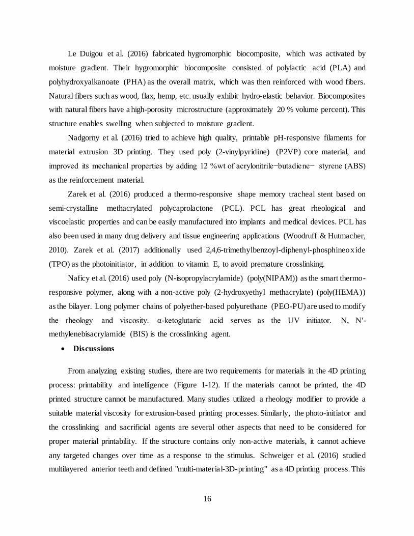
Le Duigou et al. (2016) fabricated hygromorphic biocomposite, which was activated by

moisture gradient. Their hygromorphic biocomposite consisted of polylactic acid (PLA) and

polyhydroxyalkanoate (PHA) as the overall matrix, which was then reinforced with wood fibers.

Natural fibers such as wood, flax, hemp, etc. usually exhibit hydro-elastic behavior. Biocomposites

with natural fibers have a high-porosity microstructure (approximately 20 % volume percent). This

structure enables swelling when subjected to moisture gradient.

Nadgorny et al. (2016) tried to achieve high quality, printable pH-responsive filaments for

material extrusion 3D printing. They used poly (2-vinylpyridine) (P2VP) core material, and

improved its mechanical properties by adding 12 %wt of acrylonitrile−butadiene− styrene (ABS)

as the reinforcement material.

Zarek et al. (2016) produced a thermo-responsive shape memory tracheal stent based on

semi-crystalline methacrylated polycaprolactone (PCL). PCL has great rheological and

viscoelastic properties and can be easily manufactured into implants and medical devices. PCL has

also been used in many drug delivery and tissue engineering applications (Woodruff & Hutmacher,

2010). Zarek et al. (2017) additionally used 2,4,6-trimethylbenzoyl-diphenyl-phosphineoxide

(TPO) as the photoinitiator, in addition to vitamin E, to avoid premature crosslinking.

Naficy et al. (2016) used poly (N-isopropylacrylamide) (poly(NIPAM)) as the smart thermo-

responsive polymer, along with a non-active poly (2-hydroxyethyl methacrylate) (poly(HEMA))

as the bilayer. Long polymer chains of polyether-based polyurethane (PEO-PU) are used to modify

the rheology and viscosity. α-ketoglutaric acid serves as the UV initiator. N, N′-

methylenebisacrylamide (BIS) is the crosslinking agent.

• Discussions

From analyzing existing studies, there are two requirements for materials in the 4D printing

process: printability and intelligence (Figure 1-12). If the materials cannot be printed, the 4D

printed structure cannot be manufactured. Many studies utilized a rheology modifier to provide a

suitable material viscosity for extrusion-based printing processes. Similarly, the photo-initiator and

the crosslinking and sacrificial agents are several other aspects that need to be considered for

proper material printability. If the structure contains only non-active materials, it cannot achieve

any targeted changes over time as a response to the stimulus. Schweiger et al. (2016) studied

multilayered anterior teeth and defined "multi-material-3D-printing" as a 4D printing process. This

17

is not the 4D printing process discussed in this study because the structure does not contain any

smart material.

Some applications require dual-responsive materials. For example, the shape-shifting

behavior of a material can be triggered by both water and heat. Triple and other multi-respons ive

materials have not been considered in the 4D printing process so far and can be studied in the

future. Another issue is the degree to which the smart materials can respond to stimulus. Some

smart materials can sense stimulus but only provide minimal actuation or respond after a very long

time. The responsivity of smart materials needs to be further studied as well.

Figure 1-12. 4D printing materials.

1.4 Shape-shifting mechanisms and Stimuli

A 4D-printed structure can alter its shape, properties, or functionality based on one or more

stimuli. However, an interaction mechanism needs to be identified, through which the printed

smart structure can respond to stimulus in an appropriate way. The mechanisms can be divided

into various categories. Campbell et al. (2014) explained two types of mechanisms in 4D printing:

hydro-mechanics and thermo-mechanics. In this section, other mechanisms from the literature are

organized and summarized, including unconstrained-hydro-mechanics, constrained-thermo-

mechanics, unconstrained-thermo-mechanics, unconstrained-hydro-thermo-mechanics,

unconstrained-pH-mechanics, unconstrained-thermo-photo-mechanics, osmosis-mechanics, and

dissolution-mechanics.

• Unconstrained-Hydro-Mechanics

4D printing materials

Smartness Printability

Rheology and

viscosity modifier

Requirements

Photo-initiator

agent

Crosslinking

agent

Sacrificial

agent

Considerations

Single-/ Dual-/ ...

responsiveness

Self-sensing

Decision

speed

Self-

actuating

18

In this mechanism, a smart printed structure consists of an expandable hydrophilic active

material and a passive material. Water is utilized as the external stimulus so that the structure can

undergo shape-shifting under water and so that it can return to its original shape after being dried.

This mechanism is driven by the different swelling ratios between the active and passive materials.

The expansion of the smart material generates a force that leads to the shape change. When the

expandable material is appropriately arranged with the passive material, complex shape-shifting

behavior can be achieved. The magnitude and direction of the shape change depends on the spatial

arrangements of the two materials (Tibbits et al. 2014). The mechanism is illustrated in Figure

1-13 and the entire cycle is unconstrained. Tibbits (2014), Tibbits et al. (2014), Raviv et al. (2014),

and Jamal et al. (2013) used this type of mechanism in their experiments.

It should be noted that this mechanism is naturally reversible, i.e., the original shape can be

recovered by drying the smart structure. However, the shape-shifting behavior can also be forced

to be irreversible by using a special arrangement of passive and active materials. For example,

Tibbits et al. (2014) reported that the structure in Figure A-31 will not unfold after being dried

because of geometrical constraints.

Figure 1-13. Schematic illustration of the unconstrained-hydro-mechanics mechanism in

4D printing. The green parts represent e xpandable materials.

• Constrained-Thermo-Mechanics

Drying out

of water

Wetting

under

water

Unconstrained-Hydro-Mechanics

Shape 2b

Swelling Deswelling

Shape 1a

19

Two levels of temperature and one external load are required in this mechanism, as

illustrated in Figure 1-14. One temperature is higher than the critical temperature of the smart

material, such as its glass transition temperature or crystal-melt transition temperature (𝑇𝐻 > 𝑇𝐶).

The other temperature should be lower than the critical temperature (𝑇𝐿 < 𝑇𝐶). In this mechanism,

the printed structure is heated to 𝑇𝐻 and the cycle starts at 𝑇𝐻 in the following order. First, the

original structure is stretched at 𝑇𝐻 with a certain amount of strain depending on specific

applications. Then, under external stress, the structure is cooled to 𝑇𝐿 while the strain remains

unchanged. Next, the external stress is removed at 𝑇𝐿, and the desired temporary shape is obtained

at the end of this step. Finally, the structure can be reheated to 𝑇𝐻 in a free stress condition to

recover its original shape.

In this mechanism, temperature is the external stimulus. Ge et al. applied this mechanism in

their experiments (Figures A-30 and A-24) (Ge et al., 2013; 2014). Wu et al. (2016) also employed

this mechanism (Figures A-13, A-14, A-15, A-16, and A-17). They used water with different

temperatures as a medium in order to transfer the heat to the printed structure. It should be noticed

that the temperature is still the only stimulus in this cycle to trigger the shape-shifting behavior.

Mao et al. (2015) applied this mechanism in their sequential self-folding multi-shape memory

structure (Figure A-25). Yu et al. (2015) showed the feasibility of controlling the multi-shape-

shifting sequence in a shape memory polymer based on this mechanism. Monzón et al. (2016)

experimentally studied the correlations between the amount of recovery force and the

mass/thickness/width of the printed shape memory polymers. These correlations can be effectively

applied in the 4D printing process and should be the focus of future studies on interaction

mechanisms.

20

Figure 1-14. Constrained-thermo-mechanics mechanism in 4D printing.

• Unconstrained-Thermo-Mechanics

Unlike the previous mechanism, the external load is not included in the cycle of this

mechanism. Only the two temperatures are required. One is higher than critical temperature of the

active material involved in the structure (𝑇𝐻 > 𝑇𝐶), and the other one is lower than the critical

temperature (𝑇𝐿 < 𝑇𝐶). As shown in Figure 1-15, the printed structure is first heated to 𝑇𝐻. The

cycle then starts at 𝑇𝐻 and proceeds in the following manner. First, the original structure is cooled

to 𝑇𝐿, where the desired shape is achieved at the end of this step. Then, the structure can be heated

to 𝑇𝐻 to recover its original shape. In this mechanism, the external stimulus is temperature. Zhang

et al. (2016) used this mechanism in their 4D printing studies (Figure A-26). They demonstrated

several kinds of shape-shifting behaviors in smart, lightweight, and thin composite structures, such

as transformation from a planar sheet to flower-like 3D structures, periodic 3D structures, and

adaptive metamaterials.

Heat to

TH

Unload

Original Shape at TH >TC

TH

TL

TL < TCDesired Shape at

a

b

c

d

Constrained-Thermo-Mechanics

Stretch

Cool to

TL

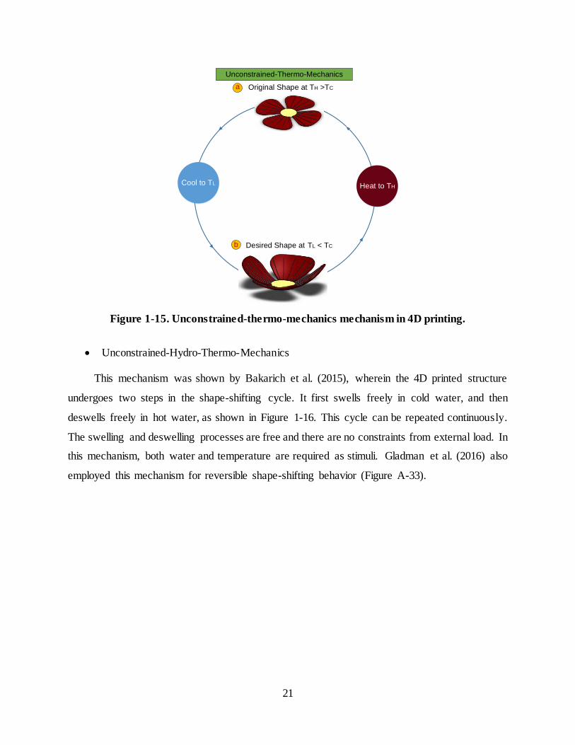
21

Figure 1-15. Unconstrained-thermo-mechanics mechanism in 4D printing.

• Unconstrained-Hydro-Thermo-Mechanics

This mechanism was shown by Bakarich et al. (2015), wherein the 4D printed structure

undergoes two steps in the shape-shifting cycle. It first swells freely in cold water, and then

deswells freely in hot water, as shown in Figure 1-16. This cycle can be repeated continuously.

The swelling and deswelling processes are free and there are no constraints from external load. In

this mechanism, both water and temperature are required as stimuli. Gladman et al. (2016) also

employed this mechanism for reversible shape-shifting behavior (Figure A-33).

Heat to THCool to TL

Original Shape at TH >TC

TL < TCDesired Shape at

a

b

Unconstrained-Thermo-Mechanics

22

Figure 1-16. Unconstrained-hydro-thermo-mechanics mechanism in 4D printing.

• Unconstrained-pH-Mechanics

This mechanism was demonstrated by Nadgorny et al. (2016). In this mechanism, a 4D-

printed, pH-responsive hydrogel can linearly swell at a specific pH level and then shrink at another

designed pH level (Figure 1-17). This cycle is mainly conducted in an aqueous environment and

is therefore suitable for the shape-shifting of hydrogels. Many studies on pH-responsive hydrogels

have been conducted in available literature (Puranik et al., 2016; Frohm et al., 2015; Krogsgaard

et al., 2013; Best et al., 2013; Gong et al., 2016). Nadgorny et al. (2016) provided pH-responsive

hydrogels with a composition appropriate for printing.

Hot

Water

Cold

Water

Shape 1a

Unconstrained-Hydro-Thermo-Mechanics

Shape 2b

Swelling Deswelling

23

Figure 1-17. Unconstrained-pH-mechanics mechanism in 4D printing.

• Unconstrained-Thermo-Photo-Mechanics

This mechanism has been demonstrated by Kuksenok et al. (2016). In this mechanism, fibers

were considered to be photo-responsive materials and the matrix was considered to be a thermo-

responsive material. They showed that the application of light, heat, or a combination of both

stimuli could yield printed structures with various morphologies. In their study, the gel has a lower

critical solution temperature and shrinks at a high temperature. The spiro benzopyran (SP)

chromophores functionalize elastic fibers, which can be converted into a hydrophobic form when

subjected to blue light, and recover its hydrophilic form in dark environments.

Different behavior under exposure to light or heat is a result of local and global response.

Light can be used to non-invasively enable local shape-shifting behavior in specific regions of the

structures (Kuksenok et al. 2016). The original composite (Figure 1-18 (a)) shrinks like an

accordion (Figure 1-18(b)) when heated freely (unconstrained) and bends like a caterpillar (Figure

1-18 (c)) when subjected to blue light. Figure 1-18(d) shows the behavior of the composite when

both heat and blue light are applied.

pH xpH < x

Unconstrained-pH-Mechanics

Shape 2b

Swelling Deswelling

Shape 1a

24

Figure 1-18. Illustration of the unconstrained-thermo-photo-mechanics mechanism.

• Osmosis-Mechanics

Villar et al. (2013) demonstrated this mechanism with a lipid interface bilayer, which joins

two picoliter aqueous droplets with two different osmolarities. Water is the stimulus in this

mechanism. The droplet with the higher osmolarity swells and the droplet with the lower

osmolarity shrinks until they reach the same osmolarity (Figure 1-19(a)), which enables self-

bending and is similar to the nastic movements of plants. At the macroscopic level, water flows

through a network of droplets and causes the network to bend in a predetermined way, as shown

in Figure 1-19(b). The final configuration of the network is determined based on the original

geometry, the spatial arrangement of the droplets, and the ratio between their osmolarities.

Hea

t & L

igh

t

Thermo-Responsive

Matrix with Photo-

Responsive Fibers

Local Response Global Response

Global and Local Responses

Unconstrained-Thermo-Photo-Mechanics

a

bc

d

25

Figure 1-19 (a) Osmosis effect between two droplets, (b) Macroscopic deformation arising

from osmosis effect (Villar et al. 2013).

• Dissolution-Mechanics

This mechanism was demonstrated by Kokkinis et al. (2015) in the field of bioprinting. In

this mechanism, a printed structure is immersed in an appropriate solvent (ethyl acetate), based on

the studied polymer structures. A change in shape occurs as a result of the loss of some non-

crosslinked polymers when the structure is immersed in the solvent. After complete drying, the

soft phase shrinks. This shape-shifting behavior is reversible by re-immersing the structure in the

solvent. In this mechanism, the appropriate solvent is the stimulus.

As a summary of this section, all the shape-shifting mechanisms and stimuli are categorized

in Figure 1-20, along with their related studies.

26

Figure 1-20. Shape-shifting mechanisms and stimuli which were used in 4D printing.

1.5 Mathematics

In this section, forward and inverse problems are defined for the 4D printing process, and

one example is provided for each category. In addition, some studies focused specifically on the

mathematics of 4D printing are discussed.

The development of the 4D printing process relies on appropriate mathematical modeling

(Gladman et al., 2016). In fact, mathematics is necessary in 4D printing for the following reasons:

• It is needed to predict the shape evolution over time after printing.

• It provides the theoretical models needed to avoid collisions between components of the

structure during the self-assembly operation.

• It reduces the number of trial-and-error experiments. Early experiments in 4D printing

involve many repetitions for a specific structure to achieve the desired shape. For example,

Tibbits et al. (2014) printed and repeated a series of experiments to identify the appropriate

• Tibbits (2014)

• Jamal et al. (2013)

• Tibbits et al. (2014)

• Raviv et a1. (2014)

• Ge et al. (2013)

• Ge et al. (2014)

• Mao et al. (2015)

•Yu et al. (2015)

• Wu et al. (2016)

• Ge et al. (2016)

•Bodaghi et al. (2016)


• Villar et al. (2013)


Shape Shifting Mechanisms and Stimuli

Unconstrained-Hydro-Mechanics

Constrained-Thermo-Mechanics

Unconstrained-Thermo-Mechanics

Unconstrained-Hydro-Thermo-Mechanics

• Bakarich et al. (2015)

• Gladman et al. (2016)

• Naficy et al. (2016)

Unconstrained-Photo-Thermo-Mechanics

Unconstrained-pH-Mechanics •Nadgorny et al. (2016)

• Kuksenok et al. (2016)

Dissolution-Mechanics

Osmosis-Mechanics

27

material structure needed to reach the desired shape. This is shown in Figure 1-21. With

mathematics and some theoretical models, the final shape can be predicted for a given

material structure, material properties, and stimulus properties. Consequently, the number

of test experiments can be reduced dramatically.

Several modeling experiments were conducted for 4D printing. The aforementioned

experimental study by Tibbits et al. (2014) was quantified with mathematical models developed

by Raviv et al. (2014), where the spring-mass concept was adopted, as shown in Figure 1-22. In

addition, this spring-mass system for shape-memory materials was also used by Sun et al. (2012)

and Yu et al. (2012). Sun et al. (2010) proposed a framework to illustrate the underlying physics

in the thermo-responsive multi-shape memory effect (multi-SME). Their study qualitative ly

investigated the energy storage and release process achieved during the shape memory cycle. Yu

et al. (2012) improved the previous qualitative study by proposing a quantitative analysis for multi-

SME, as shown in Figure 1-23. They verified their model with the experimental results for

perfluoro sulphonic acid ionomer (PFSA) from Xie (2010). Yu et al. (2012) employed the 1D

standard linear solid (SLS) model proposed by Qi et al. (2010) to illustrate the multiple relaxation

processes of the polymer chains in their multi-branch model. The SLS model has a parallel

arrangement consisting of one elastic spring and one Maxwell element. The Maxwell element

contains a serial arrangement of one spring and one dashpot. A previous study conducted on this

subject yielded a four-element model developed by Tobushi et al. (1997), in which the creep

phenomenon was incorporated through the fourth element , 𝜀𝑠 called the creep recovery strain

(Figure 1-24).

Figure 1-21. Repeated tests to identify the appropriate material structure to reach the

precise desired shape (Tibbits et al., 2014).

28

Figure 1-22. Mathematical modeling of the 4D-printed hinge that was introduced earlier by

Tibbits et al. (2014) with the spring-mass concept (Raviv al. 2014).

Figure 1-23. Standard linear solid (SLS) model to explain the mechanism of the shape

memory effect in a shape memory polymer (Yu et al. 2012).

Figure 1-24. Four-element modeling of shape memory effect (Tobushi et al. 1997).

29

An appropriate theoretical model for 4D printing consists of four major components. The

first is the final desired shape, which may include desired bending angle, twisting angle, length,

etc. The next is material structure, such as the volume fractions of fibers and the matrix, filament

size, orientation, spacing, anisotropy. Equivalently the material structure can be described by the

size, shape and spatial arrangement of the voxels. From the perspective of the printing process, the

material structure depends on print paths and nozzle sizes. Material properties makeup the third

component, and they include shear modulus, Young s modulus, and the interactive properties

associated with the stimulus, such as glass transition temperature and swelling ratio. The final

component is the stimulus properties, such as the temperature value and light intensity.

4D printing mathematics can be divided into two categories according to Gladman et al.

(2016): the forward problem and the inverse problem. The categories are defined below:

Forward problem: Determination of the final desired shape given material structures,

material properties, and stimulus properties.

Inverse problem: Determination of the material structure or the print paths and nozzle sizes

given the final desired shape, material properties, and stimulus properties.

The studies on 4D printing related to the inverse problem are application-oriented, meaning

that they are focused on achieving a desired functionality or shape. Studies related to the forward

problem are mainly fundamental research aimed toward discovering concepts, theories, and

relationships. These are illustrated in Figure 1-25.

30

Figure 1-25. 4D printing mathematics allows theoretical models to connect the final desired

shape, material structure (or equivalently the size, shape and spatial arrangement of the

voxels or equivalently print paths and nozzle sizes), material properties, and stimulus

properties.

The example with the spring-mass mathematical model shown above can be considered to

be a forward problem. Gladman et al. (2016) studied a bilayer structure and utilized the

mathematical relationships of coordinate system transformations to identify the print paths (Figure

1-29); this is an example of an inverse problem. As shown in Figure 1-26(a), the print path of the

first layer aligns along the 𝑒𝑥 direction (unit vector in x direction) and the print path of the second

layer aligns along the direction of cos(𝜃) 𝑒𝑥 + sin(𝜃)𝑒𝑦, where 𝜃 is the angle between the two

layers. The relationship between 𝜃 and the final desired shapes is then established, as given by the

following equations:

𝐻 = 𝑐1𝛼∥ −𝛼⊥ℎ

𝑠𝑖𝑛2(𝜃)

𝑐2 − 𝑐3 cos(2𝜃) + 𝑚4 cos(4𝜃)

𝐾 = −𝑐4(𝛼∥ − 𝛼⊥)

2

ℎ2𝑠𝑖𝑛2(𝜃)

𝑐5 − 𝑐6 cos(2𝜃) + 𝑚4 cos(4𝜃)

4D printing

Mathematics

Final Desired Shape

(such as desired bending

angle, desired twisting

angle, desired length,

desired volume, etc.)

Material Properties

(such as longitudinal

Young`s modulus,

transverse Young`s

modulus, swelling ratios,

glass transition

tempretaure etc.)

Stimulus Properties

(such as magnitude of

temperature, light

intensity, etc.)

Material Structure

or equivalently print paths and

nozzle sizes or equivalently the

size, shape and spatial

arrangement of the voxels

(such as volume fractions of fibers

and matrix, filament size, orientation,

and interfilament spacing, anisotropy,

etc.)

Forward problem: Final desired shape is unknown

Inverse problem: Material structure or equivalently print paths and nozzle sizes is unknown

31

where the final desired shapes are quantified by the curvature tensor 𝜿, mean curvature 𝐻 =

1

2𝑇𝑟(𝜿) =

1

2(𝜅𝑥𝑥 +𝜅𝑦𝑦) and Gaussian curvature 𝐾 = 𝐷𝑒𝑡 (𝜿) = 𝜅𝑥𝑥𝜅𝑦𝑦− 𝜅𝑥𝑦

2 , as shown in

Figure 1-26(b). 𝛼∥ and 𝛼⊥ are the longitudinal and transverse swelling strains, respectively, as

shown in Figure 1-26. 𝑚 =𝑎𝑏𝑜𝑡𝑡𝑜𝑚

𝑎𝑡𝑜𝑝 is the ratio of layer thicknesses, ℎ = 𝑎𝑡𝑜𝑝+ 𝑎𝑏𝑜𝑡𝑡𝑜𝑚 is total

thickness of the bilayer, and 𝑐𝑖 are functions of longitudinal Young s modulus , 𝐸∥ , transverse

Young s modulus, 𝐸⊥, Poisson s ratio, 𝜈 , and 𝑚. Based on final desired shape, the print paths can

be calculated accordingly. As shown in Figure 1-27 and Figure 1-28, surfaces with positive

Gaussian curvature can be produced with the concentric circles. Surfaces with negative Gaussian

curvature or saddle-like surfaces can be produced with an orthogonal bilayer lattice structure. The

combination of these two print paths can then yield a structure with varying Gaussian curvatures.

Figure 1-26. Mathematical modeling can make a connection between (a) print paths

quantified by the angle 𝜽 between the two layers, and (b) final desired shape quantified by

curvature tensor 𝜿, mean curvature 𝑯, and Gaussian curvature 𝑲(Gladman et al., 2016).

Figure 1-27. Longitudinal and transverse swelling strains (𝜶∥ and 𝜶⊥) (Gladman et al.,

2016).

32

Figure 1-28. Print paths and final shapes (a) positive Gaussian curvature (b) negative

Gaussian curvature (c) and varying Gaussian curvature (Gladman et al., 2016).

Figure 1-29. Using the concepts of the mean curvature, 𝑯, and Gaussian curvature, 𝑲,

generates the print paths by knowing the final desired morphologies (Gladman et al.,

2016).

Kowk et al. (2015) conducted design optimization of origami for freeform surfaces in 4D

printing. According to them, the 3D structure needs to be flattenable to achieve self-folding shape-

shifting. A flattenable 3D structure can be flattened into a 2D form without stretching. However,

many designed parts are not flattenable. To address this issue, they provided a geometry

optimization method, which can modify a non-flattenable pattern into a flattenable pattern. Wang

et al. (2017) studied the mathematics of the single-loop foldable 8R (revolute joint) with multiple

modes, which is also related to folding. They mathematically described that a self-folding structure

can be folded into the same pattern through different methods and can also be folded to different

patterns. These studies serve as the mathematical tools for the forward and inverse problems in 4D

printing processes.

33

1.6 Conclusions

4D printing is the art of combining science with engineering technology. The scientific

aspect of 4D printing is related to fundamental research into developing new smart materials,

stimuli, and mathematical modeling. From the engineering aspect, the 4D printing process enables

innovative and fascinating applications that can hardly be achieved with conventional

manufacturing processes. The foundation of the 4D printing process includes the 3D printing

process, stimulus, smart or stimulus-responsive materials, interaction mechanisms, and

mathematical modeling. These features enable changes in shape/property/functionality after

printing, as a function of time.

In addition, 4D printing has three main capabilities: self-assembly, self-adaptability, and

self-repair. More studies need to be performed in the area of self-repair compared with the other

two. Mathematical modeling is necessary in the 4D printing process primarily for three reasons:

the prediction of the shape-shifting as a function of time; the prevention of collisions between

components of the structure during self-assembly operations, and finally, the reduction of the

number of trial-and-error experiments. The mathematical models used in the 4D printing process

can be developed based on a desired shape, printing path, material properties, and stimulus

properties. 4D printing can be utilized in various scales in interesting applications. To gain the

potential applications of the 4D printing, a large amount of multidisciplinary research needs to be

conducted in the future.

1.7 Problem statement and dissertation structure

After a comprehensive review of the 4D printing and related areas, three substantial gaps are

identified in this emerging field. First, the main difference between 3D and 4D printed structures

is one extra dimension that is smart evolution over “time”. However, currently, there is no general

formula to model and predict this extra dimension. This gap is related to the design aspect of 4D

printing. Second, 3D printing (additive manufacturing) is a manufacturing process with its known

unique attributes. Now, 4D printing needs to be clearly underpinned as a new manufacturing

process. Unique attributes of 4D printing as a new manufacturing process should also be identified.

This gap is related to the manufacturing aspect of 4D printing. Third, various shape-morphing 4D

printed structures have been illustrated in the literature. However, real applications and products,

in which 4D printing can provide unique features still need to be demonstrated. 4D printing is not

34

just a concept, it is also a manufacturing paradigm that finally should lead to useful and applicable

products or structures. Thus, real applications that can benefit from 4D printed structures should

be addressed, continuously. This gap is related to the product development aspect of 4D printing.

To address the first gap (design), we have the second chapter, where we present general

design principles of 4D printing that are required for understanding, modeling, and predicting the

shape-shifting behaviors (the 4th D) of any multi-material 4D printed structure. To address the

second gap (manufacturing), we have the third chapter, where we clearly underpin 4D printing as

a new manufacturing process and specifically work on its energy-saving characteristic and obtain

its theoretical limit. To address the third gap (product development), we have the fourth and fifth

chapters, where we demonstrate two real applications (one in solar energy and one in wind energy),

in which 4D printed products can provide unique benefits. These three main gaps and their

corresponding chapters are related to design, manufacturing, and product development aspects of

4D printing.

35

CHAPTER 2

LAWS OF SHAPE-SHIFTING IN 4D PRINTING

The main difference between 3D and 4D printed structures is one extra dimension that is

smart evolution over “time”. However, currently, there is no general formula to model and predict

this extra dimension. Here, by starting from fundamental concepts, we derive and validate a

general bi-exponential formula that can model and predict the fourth D of 4D printed multi-

material structures. 4D printing is a new manufacturing paradigm that utilizes stimuli-respons ive

materials in multi-material structures for advanced manufacturing (and construction) of novel

products (and structures). It conserves the general attributes of 3D printing (such as the elimination

of molds, dies, and machining) and further enables the fourth dimension of products and structures

to provide intelligent behavior over time.

This intelligent behavior is encoded (usually by an inverse mathematical problem) into

stimuli-responsive multi-materials during printing and is enabled by stimuli after printing. Here,

we delve into the fourth dimension and reveal three general laws that govern the time-dependent

shape-shifting behaviors of almost “all” (photochemical-, photothermal-, solvent-, pH-, moisture-,

electrochemical-, electrothermal-, ultrasound-, enzyme-, etc.-responsive) multi-material 4D

structures. We demonstrate that two different types of time-constants govern the shape-shifting

behavior of almost all the multi-material 4D printed structures over time. Our results starting from

the most fundamental concepts and ending with governing equations can serve as general design

principles for future research in the 4D printing field, where the “time-dependent” behaviors

should be understood, modeled, and predicted correctly. Future software and hardware

developments in 4D printing can also benefit from these results.2

2 This chapter is based on our journal article (under review), entitled “Laws of 4D printing”, by Farhang Momeni and

Jun Ni.

36

2.1 Introduction

Although some studies demonstrated single-material 4D printed structures, the future of 4D

printing will lie in multi-material structures (Tibbits, 2014; Raviv et al., 2014; Ge et al., 2016; Pei

& Loh, 2018; Kwok & Chen, 2017; Lind et al., 2017; News Staff, accessed 2018; Major, accessed

2018; Saunders, accessed 2018). The quiddity of 4D printing usually needs multi-materia l

structures (Raviv et al., 2014). In the most fundamental case, the multi-material 4D printed

structure has one active and one passive layer (Kwok & Chen, 2017). Performance improvement

by allocating proper materials to related locations based on local necessities (Bandyopadhyay &

Heer, 2018), multi-functionality by embeddable functions such as electronics (MacDonald &

Wicker, 2016), combing rigid and flexible sections in an integrated structure (Lopes et al., 2018),

and providing lightweight structures (Demir & Previtali, 2017) are only some of the advantages of

multi-material structures.

In addition, to enable the shape memory effect (SME) (that is not an intrinsic property (Behl

& Lendlein, 2007) of shape memory polymers (SMPs), a mechanical force is required in addition

to heat (thermomechanical cycles). This force is usually provided externally. However, 4D printing

can help us to arrange active and passive materials in a multi-material structure and utilize their

internal mismatch-driven forces to enable the SME autonomously, with no need of external load

for training (Mao et al., 2016; Momeni et al., 2019). In this study, we focus on multi-material 4D

printed structures.

Aspects of 4D printing have been explored in the literature. Several studies worked on beam

and plate theories (e.g., refer to the supplementary information of ref. (Gladman et al., 2016).

However, the missing piece in the literature is modeling of “time-dependent” behaviors (the 4th D)

of 4D structures. Especially, the time-dependent behavior is the critical part of 4D (stimuli-

responsive) materials, whether fabricated by additive manufacturing and thus called 4D printed

structures or created by other manufacturing processes. More importantly, a huge number of

studies on 4D materials used the Timoshenko bimetal model (Timoshenko, 1925) (that is linear

with time) to analyze the time-dependent behaviors of their experiments. Here, we will see that, in

general, the Timoshenko bimetal model cannot capture the true time-dependent behaviors of 4D

materials (except for some special cases or selected linear regions), although it provides useful

insights on time-independent behaviors. In fact, the purpose of Timoshenko bimetal model was

37

not to model the time-dependent behavior (the 4th D) of 4D materials. Thus, there is an urgent need

for qualitative and quantitative analysis on the 4th D of 4D materials.

The main part of 4D printed structures is the 4th D; however, currently, there is no general

formula to model and predict this extra dimension. Here, by developing fundamental concepts and

from the equilibrium and compatibility conditions, we derive a bi-exponential formula that “is

needed” for modeling and predicting the 4th D of any multi-material 4D printed structure. We

further validate our bi-exponential formula by various experimental data from separate studies in

the literature and show that it is a general formula that is useful for any type of 4D multi-materia l

structure (photochemical-, photothermal-, solvent-, pH-, moisture-, electrochemical-,

electrothermal-, ultrasound-, enzyme-, etc.-responsive). This generality happens, because we build

the bases of our bi-exponential formula, comprehensively.

2.2 Definitions, derivations, and discussions

There are many materials and stimuli. Consequently, most of the ongoing studies in the 4D

printing field are case-specific. The time-dependent behavior (the 4th D) of any 4D printed structure

needs to be predicted. A detailed, but systematic, study on 4D printing and related areas helped us

to reveal three universal laws that govern the “shape-shifting” behaviors of almost all the multi-

material 4D printed structures, although there are many materials and stimuli (Figure 2-1).

Figure 2-1. Toward the laws of shape-shifting in 4D printing.

38

2.2.1 First law

Almost all the shape-shifting behaviors (photochemical-, photothermal-, solvent-, pH-,

moisture-, electrochemical-, electrothermal-, ultrasound-, enzyme-, hydro-, thermo-, etc.-

responsive) of the multi-material 4D printed structures originate from one fundamental

phenomenon that is “relative expansion” between active and passive materials.

This “relative expansion” is the origin of almost all the complicated 4D printing shape-

shifting behaviors such as twisting, coiling, curling, etc., that are enabled by encoding various

types of anisotropy between active and passive materials and fabricating different heterogeneous

structures.

2.2.2 Second law

The shape-shifting behaviors of almost all the multi-material 4D printed structures have four

different types of physics: mass diffusion, thermal expansion/contraction, molecular

transformation, and organic growth. They all (discussed and quantified below) lead to the relative

expansion between active and passive materials and consequent shape-shifting behaviors under

stimuli (the stimulus is usually provided externally, but it can be internal).

2.2.2.1 Quantifying the second law

Here, we describe and quantify the four underlying physical concepts that lead to relative

expansions between active and passive materials in multi-material 4D structures, resulting in

various shape-shifting behaviors, with or without shape memory effect.

2.2.2.1.1 Mass Diffusion

In this category, a matter transport leads to the relative expansion.

Mass change due to sorption (absorption or adsorption) of a guest matter (here is mainly a

stimulus such as water, ion, etc.) in a host matter can be modeled as below (Kim et al., 2003;

Berens & Hopfenberg, 1978; Czugala et al., 2014):

where 𝑡 is time and 𝑀 is mass. 𝐶 and 𝜏 are usually obtained by curve fitting to experimental

data and depend on host matter relaxation and guest matter diffusion. However, models can be

developed for these two parameters. The exponential model above captures the correct behavior

of mass diffusion for short- to long-time processes. There is also one other model called power

∆𝑀

𝑀(𝑡) = 𝐶 [1− exp (−

𝑡

𝜏)], (2-1)

39

function (𝑘𝑡𝑛), which is not accurate for long-time processes of mass diffusion (Kim et al., 2003).

However, we know that the main part of 4D printing is the intelligent behavior over “time” that

can be short or long.

The exponential model above has been mainly introduced for ∆𝑀

𝑀 and

∆𝑉

𝑉 (volumetric strain).

However, we have

where 𝑉 is volume, 𝐿 is length, 𝜀 is strain, and the second- and third-order differential

quantities are neglected.

For an isotropic material,

In addition, mass and volume have a linear relationship. Therefore,

where 𝐶1 and 𝜏1 are constants that depend on the previous parameters.

We quantify all the four categories in terms of strain. One reason is that for example, if we

want to quantify them in terms of mass, then we do not have any mass change in the next category

(Thermal Expansion/Contraction). Similarly, we do not have temperature change in this category,

while we have it in the next category.

In this category, several stimuli can be used such as hydro-, solvent-, moisture-, pH-,

enzyme-, photochemical-, and electrochemical-responsive mechanisms. All of these stimuli finally

cause a matter transport, leading to relative expansion in multi-material 4D structures, resulting in

various shape-shifting behaviors.

2.2.2.1.2 Thermal Expansion/Contraction

In this category, a temperature change will increase (or decrease) the average distance

between atoms and molecules (with constant mass), leading to the relative expansion in multi-

materials.

Strain due to temperature change is (Pytel & Kiusalaas, 2012):

∆𝑉

𝑉=𝑉2 − 𝑉1𝑉

=(𝐿𝑥 + ∆𝐿𝑥)(𝐿𝑦+∆𝐿𝑦)(𝐿𝑧+ ∆𝐿𝑧) − 𝐿𝑥𝐿𝑦𝐿𝑧

𝐿𝑥𝐿𝑦𝐿𝑧≅ 𝜀𝑥 + 𝜀𝑦+ 𝜀𝑧 , (2-2)

𝜀𝑥 = 𝜀𝑦 = 𝜀𝑧 = 𝜀 ⇒ 𝜀 =1

3

∆𝑉

𝑉. (2-3)

𝜀Mass Diffusion(𝑡) = 𝐶1 [1 − exp (−𝑡

𝜏1)], (2-4)

𝜀thermal = 𝛼∆𝑇, (2-5)

40

where 𝛼 is thermal expansion coefficient and 𝑇 is temperature. Because we need to predict

the behavior of 4D printed structures over time, we convert this temperature-based equation to

time-based form.

On the other hand, by applying a thermal stimulus with temperature 𝑇2 to a structure with

temperature 𝑇1 , and assuming a uniform temperature in the structure, the temperature of the

structure changes over time as below (Kaviany, 2011):

where 𝑡 is time, 𝑇1(𝑡 = 0) is the initial temperature of the structure, ��1 is energy conversion

in the structure, 𝑄1 is the heat transferred between the structure and environment (other than the

stimulus), and 𝑅 is thermal resistance. 𝜏 is a time-constant that depends on density, heat capacity,

volume of the structure, and thermal (and thermal contact) resistance, and can be modeled in a

specific application (Kaviany, 2011).

By working on the above equation, we have

𝑇1(𝑡) − 𝑇1(𝑡 = 0)

= [𝑇2 − 𝑇1(𝑡 = 0)] − [𝑇2 − 𝑇1(𝑡 = 0)]exp (−𝑡

𝜏) +𝑅(��1− 𝑄1) [1− exp (−

𝑡

𝜏)],

⇒ 𝑇1(𝑡) − 𝑇1(𝑡 = 0) = [𝑇2 −𝑇1(𝑡 = 0)][1 − exp (−𝑡

𝜏)] + 𝑅(��1 − 𝑄1) [1− exp (−

𝑡

𝜏)],

⇒ 𝑇1(𝑡) − 𝑇1(𝑡 = 0) = [𝑇2 −𝑇1(𝑡 = 0) +𝑅(��1 −𝑄1)][1 − exp (−𝑡

𝜏)],

By combining the above equation and the initial equation (i.e., 𝜀 = 𝛼∆𝑇), we will have


In this category, several stimuli can be used such as photothermal-, electrothermal-, and

ultrasound- responsive mechanisms. All of these stimuli finally raise the temperature of the

structure and consequently, increase the average distances between atoms and molecules. For

example, in electrothermal-responsive structures, the movement of a current through a resistance

provides heat (so-called Joule or Ohmic heating), this heat increases the temperature, and finally,

the expansion happens. Similarly, contraction is obtained by cooling. It should be noted that some

𝑇1(𝑡) = 𝑇2 + [𝑇1(𝑡 = 0) − 𝑇2]exp (−𝑡

𝜏) +𝑅(��1 − 𝑄1) [1− exp (−

𝑡

𝜏)], (2-6)

⇒ ∆𝑇1 = [𝑇2 − 𝑇1(𝑡 = 0) + 𝑅(��1 − 𝑄1)] [1− exp (−𝑡

𝜏)]. (2-7)

𝜀Thermal Expansion/Contraction(𝑡) = 𝐶2[1 − exp (−𝑡

𝜏2)], (2-8)

41

materials will shrink (contract) upon heating. In these cases, 𝛼 (the thermal expansion coefficient)

would be negative in the equations above and the final equation, i.e.,

𝜀Thermal Expansion/Contraction (𝑡) = 𝐶2 [1 − exp (−𝑡

𝜏2)] will remain intact. Nevertheless, the key

point is the “relative” thermal expansion/shrinkage in multi-materials to enable various shape-

shifting behaviors in this category.

2.2.2.1.3 Molecular Transformation

In this category, a molecular transformation (e.g., trans-to-cis change in azobenzene) with

constant mass and temperature leads to the relative expansion. The constant-temperature feature

of this category indicates that the relative expansion is not due to the thermal expansion/contraction ,

even though some thermal fluctuation may happen in the structure due to bond cleavage or

formation.

The molecular transformation is usually accomplished by photochemical responsivity

mechanism that is different from photothermal responsivity (Naumov et al., 2015). The kinetics of

photoinduced transformation is (Naumov et al., 2015):

where 𝑡 is time and 𝐷(𝑡) is the degree of transformation. 𝐷0 and 𝜏 are constants that depend

on the irradiation flux intensity, quantum yield of the transformation, etc., and can be modeled in

a specific application (Naumov et al., 2015).

On the other hand, subsequent volume change (expansion or contraction) is proportional to

the degree of transformation (Naumov et al., 2015). In addition, we have already seen that the

volumetric strain (∆𝑉

𝑉) and linear strain (𝜀 =

∆𝐿

𝐿) are proportional. Therefore,


The main stimulus for this category is the photochemical-responsive mechanism.

2.2.2.1.4 Organic Growth

In this category, there is a living layer (organism) and its growth over time can lead to the

relative expansion between active and passive materials. The organic growth can be defined as the

increase of an organic system in weight or length (Von Bertalanffy, 1938). This usually happens

𝐷(𝑡) = 𝐷0[1 − exp (−𝑡

𝜏)], (2-9)

𝜀Molecular Transformation(𝑡) = 𝐶3[1 − exp (−𝑡

𝜏3)], (2-10)

42

in bioscience and bioengineering dealing with cells, soft tissues, organs, scaffolds, and so on that

can be 4D printed and are generally called 4D bioprinting.

Kinetics of the organic growth is (Von Bertalanffy, 1938):

where 𝑡 is time, 𝐿(𝑡) is the length of the organic system, 𝐿∞ is the final length, and 𝐿0 is the

initial length. 𝜏 is usually a curve-fitting time-constant that depends on the metabolism of the living

organism, environment, and so on. Nevertheless, models can be developed for it. It should also be

noted that 𝜏 affects 𝐿∞ (Von Bertalanffy, 1938). This formula shows the growth of individual

organisms in a population that is different from population growth. The population growth is the

growth in the number of individuals in a population and is modeled by other formulas (Malthus,

1798; Verhulst, 1838).

On the other hand, based on the definition of strain, 𝜀 =𝐿(𝑡)−𝐿0

𝐿0, we have

Therefore,


In this category, one of the main stimuli that can trigger a living organism would be the

electrical signal (electrochemical mechanism). In addition, various stimuli such as pH, light, heat,

and enzyme can be used to tune the growth rate.

2.2.2.2 Unified model of the second law

By quantifying the second law, we found that

𝐿(𝑡) = 𝐿∞− (𝐿∞ − 𝐿0)exp (−𝑡

𝜏), (2-11)

𝜀 =𝐿(𝑡) − 𝐿0𝐿0

=(𝐿∞− 𝐿0) − (𝐿∞ −𝐿0) exp (−

𝑡𝜏)

𝐿0

= (𝐿∞ − 𝐿0𝐿0

)[1 − exp (−𝑡

𝜏)].

(2-12)

𝜀Organic Growth(𝑡) = 𝐶4[1 − exp (−𝑡

𝜏4)], (2-13)

43

where 𝐶𝑖 and 𝜏𝑖 (𝑖 = 1,2,3,4) all are constants. However, they depend on different factors as

described.

2.2.3 Third law

Time-dependent shape-shifting behavior of almost all the multi-material 4D printed

structures is governed by two “different types” of time-constants. For the most fundamental case

of a multi-material 4D printed structure having one active and one passive layer (Figure 2-2), the

time-dependent behavior (in terms of “curvature” that is a building block concept for shape-

shifting) is

𝜅(𝑡) =1

𝜌(𝑡) =

𝐻𝐼 (1 − 𝑒−𝑡𝜏𝐼)+ 𝐻𝐼𝐼 (1 − 𝑒

−𝑡𝜏𝐼𝐼)

ℎ2+ 2(𝐸1𝐼1 +𝐸2𝐼2)

ℎ(1𝐸1𝑎1

+ 1𝐸2𝑎2

)

= 𝐾𝐼 (1 − 𝑒−𝑡𝜏𝐼)+ 𝐾𝐼𝐼 (1 − 𝑒

−𝑡𝜏𝐼𝐼),

(2-15)

where 𝑡 is time, 𝜅(𝑡) is the curvature induced by the relative expansion, 𝜌 is the radius of

curvature, ℎ and 𝑎𝑖 are thicknesses identified in Figure 2-2, 𝐸𝑖 is Young s modulus, and 𝐼𝑖 is the

second moment of area. The passive and active layers are denoted by numbers 1 and 2, respectively.

𝐻𝐼 is a constant that depends on Young s moduli of the active and passive layers and the amount

of the mismatch-driven stress generated at the interface. 𝜏𝐼 is a time-constant that depends on the

viscosity induced at the interface and Young s moduli of the active and passive layers. The

viscosity induced at the interface needs to be measured or modeled for a specific active-passive

composite. The exact format of 𝐻𝐼 and 𝜏𝐼 can be developed in a specific application depending on

the active-passive composite and by using parallel and series rules of springs (elasticity elements)

{

𝜀Mass Diffusion(𝑡) = 𝐶1 (1 − 𝑒

−𝑡𝜏1)

𝜀Thermal Expansion/Contraction(𝑡) = 𝐶2(1 − 𝑒−𝑡𝜏2)

𝜀Molecular Transformation(𝑡) = 𝐶3 (1 − 𝑒−𝑡𝜏3)

𝜀Organic Growth(𝑡) = 𝐶4 (1 − 𝑒−𝑡𝜏4)

, (2-14)

44

and dashpots (viscosity elements). 𝐻𝐼𝐼 and 𝜏𝐼𝐼 are respectively equivalent to 𝐶𝑖 and 𝜏𝑖 (𝑖 = 1,2,3,4)

of the unified model in the previous section.

2.2.3.1 Proof of the third law

To derive equation (2-15), we start from the equilibrium and compatibility conditions that

are the starting point for any problem in mechanics of materials (Pytel & Kiusalaas, 2012). We

also consider the Timoshenko bimetal model (Timoshenko, 1925) (and its basic assumptions).

Figure 2-2. Toward the third law by analyzing the most fundamental multi-material 4D

structure.

Equilibrium:

First, we must have balances of forces and moments in Figure 2-2. Therefore (Timoshenko,

1925),

𝐵𝑎𝑙𝑎𝑛𝑐𝑒 𝑜𝑓 𝑓𝑜𝑟𝑐𝑒𝑠: ∑𝑭 = 0 ⇒ 𝑃1 = 𝑃2 = 𝑃 (2-16)

𝐵𝑎𝑙𝑎𝑛𝑐𝑒 𝑜𝑓 𝑚𝑜𝑚𝑒𝑛𝑡𝑠: ∑𝑴 = 0 ⇒ 𝑃1𝑎12+𝑃2𝑎22= 𝑀1 +𝑀2

𝑃1=𝑃2=𝑃𝑎1+𝑎2=ℎ⇒

𝑃ℎ

2

= 𝑀1 +𝑀2,

(2-17)

45

where 𝑃𝑖 and 𝑀𝑖 are forces and moments, respectively (shown in Figure 2-2).

Compatibility:

Second, at the interface of the two layers, the lengths of the two layers are the same after

applying the stimulus. Because their initial lengths are also the same, their strains must be equal

and thus (Timoshenko, 1925; Pytel & Kiusalaas, 2012),

𝐴𝑡 𝑡ℎ𝑒 𝑖𝑛𝑡𝑒𝑟𝑓𝑎𝑐𝑒: 𝜀1 = 𝜀2.

The strain in each of the two layers has three main contributors as below (Timoshenko, 1925;

Matsumoto, 2016).

(𝜀𝑐𝑢𝑟𝑣𝑎𝑡𝑢𝑟𝑒+ 𝜀𝑠𝑡𝑟𝑒𝑠𝑠 + 𝜀𝑒𝑥𝑝𝑎𝑛𝑠𝑖𝑜𝑛)1 =(𝜀𝑐𝑢𝑟𝑣𝑎𝑡𝑢𝑟𝑒 + 𝜀𝑠𝑡𝑟𝑒𝑠𝑠 + 𝜀𝑒𝑥𝑝𝑎𝑛𝑠𝑖𝑜𝑛)2. (2-18)

Strain from curvature: 𝜀𝑐𝑢𝑟𝑣𝑎𝑡𝑢𝑟𝑒

{(𝜀𝑐𝑢𝑟𝑣𝑎𝑡𝑢𝑟𝑒)1 =

𝑎1

2𝜌

(𝜀𝑐𝑢𝑟𝑣𝑎𝑡𝑢𝑟𝑒)2 = −𝑎2

2𝜌

(Timoshenko, 1925). (2-19)

Strain from stress: 𝜀 𝑠𝑡𝑟𝑒𝑠𝑠

{(𝜀 𝑠𝑡𝑟𝑒𝑠𝑠)1 =

𝑃1

𝐸1𝑎1

(𝜀 𝑠𝑡𝑟𝑒𝑠𝑠)2 = −𝑃2

𝐸2𝑎2

(Timoshenko, 1925). (2-20)

(2-18),(2-19),and (2-20)⇒

𝑎12𝜌+

𝑃1𝐸1𝑎1

+ (𝜀𝑒𝑥𝑝𝑎𝑛𝑠𝑖𝑜𝑛)1

= −𝑎22𝜌−

𝑃2𝐸2𝑎2

+ (𝜀𝑒𝑥𝑝𝑎𝑛𝑠𝑖𝑜𝑛)2.

(2-21)

Now, in the following, we develop 𝜀𝑠𝑡𝑟𝑒𝑠𝑠 and 𝜀𝑒𝑥𝑝𝑎𝑛𝑠𝑖𝑜𝑛 for 4D multi-materials and

incorporate them in the equilibrium and compatibility equations.

Here, we note that 𝜀 𝑠𝑡𝑟𝑒𝑠𝑠 is the strain due to the mismatch-driven stress at the interface of

the active and passive materials. The mismatch-driven stress naturally leads to opposing resistive

forces in the two layers (in general). We include the resistive effect by expanding the well-known

moment equation for each layer, 𝑀𝑖 . By considering Figure 2-2(c),

𝑀𝑖 = ∫𝒓𝒊 × 𝑑𝑭𝒊 = ∫𝒛𝒊𝜎𝑖𝑑𝐴𝑖

= (∫𝒛𝒊𝜎𝑖𝑑𝐴𝑖)𝑒𝑥𝑐𝑒𝑝𝑡 𝑖𝑛𝑡𝑒𝑟𝑓𝑎𝑐𝑒

+ (∫ 𝒛𝒊𝜎𝑖𝑑𝐴𝑖)𝑖𝑛𝑡𝑒𝑟𝑓𝑎𝑐𝑒

.

(2-22)

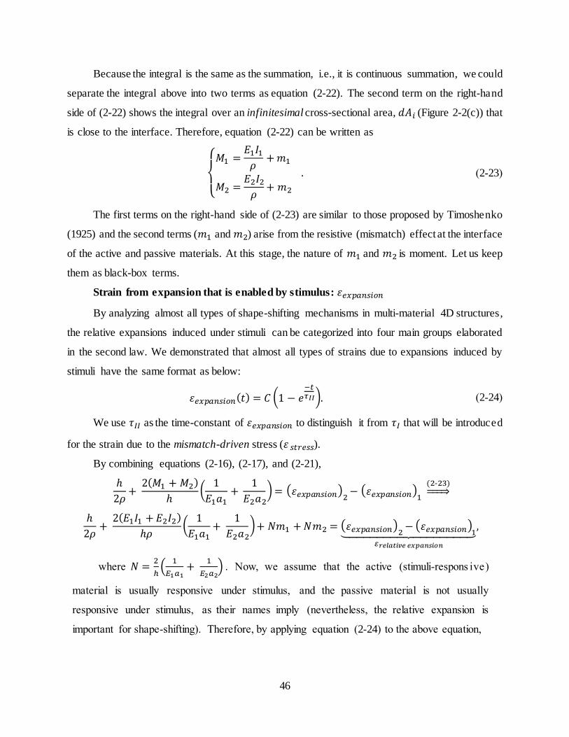
46

Because the integral is the same as the summation, i.e., it is continuous summation, we could

separate the integral above into two terms as equation (2-22). The second term on the right-hand

side of (2-22) shows the integral over an infinitesimal cross-sectional area, 𝑑𝐴𝑖 (Figure 2-2(c)) that

is close to the interface. Therefore, equation (2-22) can be written as

{

𝑀1 =𝐸1𝐼1𝜌+𝑚1

𝑀2 =𝐸2𝐼2𝜌+ 𝑚2

. (2-23)

The first terms on the right-hand side of (2-23) are similar to those proposed by Timoshenko

(1925) and the second terms (𝑚1 and 𝑚2) arise from the resistive (mismatch) effect at the interface

of the active and passive materials. At this stage, the nature of 𝑚1 and 𝑚2 is moment. Let us keep

them as black-box terms.

Strain from expansion that is enabled by stimulus: 𝜀𝑒𝑥𝑝𝑎𝑛𝑠𝑖𝑜𝑛

By analyzing almost all types of shape-shifting mechanisms in multi-material 4D structures,

the relative expansions induced under stimuli can be categorized into four main groups elaborated

in the second law. We demonstrated that almost all types of strains due to expansions induced by

stimuli have the same format as below:

𝜀𝑒𝑥𝑝𝑎𝑛𝑠𝑖𝑜𝑛(𝑡) = 𝐶 (1 − 𝑒−𝑡𝜏𝐼𝐼). (2-24)

We use 𝜏𝐼𝐼 as the time-constant of 𝜀𝑒𝑥𝑝𝑎𝑛𝑠𝑖𝑜𝑛 to distinguish it from 𝜏𝐼 that will be introduced

for the strain due to the mismatch-driven stress (𝜀 𝑠𝑡𝑟𝑒𝑠𝑠).

By combining equations (2-16), (2-17), and (2-21),

ℎ

2𝜌+ 2(𝑀1 + 𝑀2)

ℎ(1

𝐸1𝑎1+

1

𝐸2𝑎2)= (𝜀𝑒𝑥𝑝𝑎𝑛𝑠𝑖𝑜𝑛)2−

(𝜀𝑒𝑥𝑝𝑎𝑛𝑠𝑖𝑜𝑛)1 (2-23)⇒

ℎ

2𝜌+ 2(𝐸1𝐼1 +𝐸2𝐼2)

ℎ𝜌(1

𝐸1𝑎1+

1

𝐸2𝑎2)+ 𝑁𝑚1 +𝑁𝑚2 = (𝜀𝑒𝑥𝑝𝑎𝑛𝑠𝑖𝑜𝑛)2−

(𝜀𝑒𝑥𝑝𝑎𝑛𝑠𝑖𝑜𝑛)1⏟ 𝜀𝑟𝑒𝑙𝑎𝑡𝑖𝑣𝑒 𝑒𝑥𝑝𝑎𝑛𝑠𝑖𝑜𝑛

,

where 𝑁 =2

ℎ(1

𝐸1𝑎1+

1

𝐸2𝑎2) . Now, we assume that the active (stimuli-respons ive)

material is usually responsive under stimulus, and the passive material is not usually

responsive under stimulus, as their names imply (nevertheless, the relative expansion is

important for shape-shifting). Therefore, by applying equation (2-24) to the above equation,

47

ℎ

2𝜌+ 2(𝐸1𝐼1 +𝐸2𝐼2)

ℎ𝜌(1

𝐸1𝑎1+

1

𝐸2𝑎2)+ 𝑁𝑚1 +𝑁𝑚2 = 𝐶 (1 − 𝑒

−𝑡𝜏𝐼𝐼).

Now, each term in the above equation is strain. Therefore, the nature of 𝑁𝑚1 and 𝑁𝑚2

is strain. On the other hand, these two terms reflect the mismatch (viscosity) effect of the

interface into each layer. The viscoelastic strain over time can be modeled by an exponential

term as below (Duffy, 2010).

ℎ

2𝜌+ 2(𝐸1𝐼1 + 𝐸2𝐼2)

ℎ𝜌(1

𝐸1𝑎1+

1

𝐸2𝑎2)+𝐴1 (1 − 𝑒

−𝑡𝐵1 )+𝐴2 (1 − 𝑒

−𝑡𝐵2 ) = 𝐶 (1 − 𝑒


where 𝐴1 and 𝐴2 are constants that depend on Young s moduli of the active and passive

layers and the amount of the mismatch-driven stress generated at the interface. This stress is

affected by the stimulus power (such as light intensity, pH value, etc.). 𝐵1 and 𝐵2 are constants

that depend on the viscosity induced at the interface (that is related to the active-passive

composite) and Young s moduli of the active and passive layers. It should be noted that the

Young s modulus and viscosity are affected by the fabrication process (Momeni et al., 2019)

and its conditions (such as printing resolution).

On the other hand, because the two layers are attached at the interface during the shape-

shifting, 𝐵1 and 𝐵2 (time-constants of strains in each layer due to the mismatch-driven stress

at the interface) are equal (𝐵1 = 𝐵2 = 𝜏𝐼). Thus,

ℎ

2𝜌+ 2(𝐸1𝐼1 + 𝐸2𝐼2)

ℎ𝜌(1

𝐸1𝑎1+

1

𝐸2𝑎2)+𝐴1 (1 − 𝑒

−𝑡𝜏𝐼 )+𝐴2 (1 − 𝑒

−𝑡𝜏𝐼 ) = 𝐶 (1 − 𝑒


By using new uniform notations 𝐻𝐼 and 𝐻𝐼𝐼,

ℎ

2𝜌+ 2(𝐸1𝐼1 + 𝐸2𝐼2)

ℎ𝜌(1

𝐸1𝑎1+

1

𝐸2𝑎2) = 𝐻𝐼 (1 − 𝑒

−𝑡𝜏𝐼 )+𝐻𝐼𝐼 (1 − 𝑒


Finally, by re-arranging,

1

𝜌=

𝐻𝐼 (1 − 𝑒−𝑡𝜏𝐼)+ 𝐻𝐼𝐼 (1 − 𝑒

−𝑡𝜏𝐼𝐼)

ℎ2+ 2(𝐸1𝐼1 +𝐸2𝐼2)

ℎ(1𝐸1𝑎1

+ 1𝐸2𝑎2

)= 𝐾𝐼 (1 − 𝑒

−𝑡𝜏𝐼)+ 𝐾𝐼𝐼 (1 − 𝑒


which is the same as equation (2-15).

2.2.3.2 Stimulus-on versus stimulus-off

Equation (2-15) is used when the stimulus is “on”, and a curvature happens in the structure.

However, when the stimulus is “off”, the structure can return to its original shape by starting from

48

the final curvature of the previous part (i.e., the stimulus-on region). Therefore, the governing

equation for the second region can be found as below:

(1

𝜌)off

= { lim𝑡→∞

(or large 𝑡)

[𝐾𝐼 (1 − 𝑒−𝑡

𝜏𝐼)+𝐾𝐼𝐼 (1 − 𝑒−𝑡

𝜏𝐼𝐼)]} − [𝐾𝐼 (1 − 𝑒−𝑡


𝜏𝐼𝐼)]

= (𝐾𝐼 + 𝐾𝐼𝐼) − [𝐾𝐼 (1 − 𝑒−𝑡𝜏𝐼 )+𝐾𝐼𝐼 (1 − 𝑒

−𝑡𝜏𝐼𝐼)]

= 𝐾𝐼𝑒−𝑡𝜏𝐼 + 𝐾𝐼𝐼𝑒

−𝑡𝜏𝐼𝐼 . (2-25)

It should be noted that in some applications, a self-locking mechanism could be devised by

special arrangements of active and passive materials so that when the stimulus is off, the structure

does not return to its original shape.

2.2.3.3 General graph

Based on equations (2-15) and (2-25), the general graph is rendered in Figure 2-3. Some

applications need only one cycle, and some others require multiple cycles. In some applications,

only one of the two regions of the graph happens and in some other applications, both the regions

are present. In some cases, the shape-shifting behavior can occur with memory (SME), and in some

other cases, it can take place without memory.

49

Figure 2-3. The general graph that exhibits the time-dependent behavior of almost all the

multi-material 4D printed structures (photochemical-, photothermal-, solvent-, pH-,

moisture-, electrochemical-, electrothermal-, ultrasound-, enzyme-, hydro-, etc.-

responsive).

2.2.3.4 Analyzing the proposed formula by using real data

Here, we analyze our derived bi-exponential formula by using real data. For completeness,

we also consider the Timoshenko bimetal (Timoshenko, 1925) and mono-exponential models. As

seen in Figure 2-4, unlike the Timoshenko bimetal and mono-exponential models, the developed

bi-exponential model perfectly captures the correct time-dependent behavior of various

experimental data from separate studies in the literature. Therefore, in general, the time-dependent

behavior of 4D multi-materials is nonlinear (with time) and has the specific format as equation

𝜿(𝒕) = 𝑲𝑰𝐞𝐱𝐩(−𝒕/𝝉𝑰) +

𝑲𝑰𝑰𝐞𝐱𝐩(−𝒕/𝝉𝑰𝑰)

𝜿(𝒕) = 𝑲𝑰[𝟏 − 𝐞𝐱𝐩(−𝒕/𝝉𝑰)]

+𝑲𝑰𝑰[𝟏 − 𝐞𝐱𝐩(−𝒕/𝝉𝑰𝑰)]

50

(2-15). Some of the following studies presented experimental data for time-dependent curvature,

and some others provided experimental data for time-dependent angle of rotation (deflection

angle). However, the curvature and deflection angle have a linear relationship. Consequently, if

one of them has bi-exponential behavior, the other one will have bi-exponential behavior. All the

six items in Figure 2-4 have one active material and one passive material. The active component

has responsivity to the desired stimulus, whether with or without shape memory effect. We

performed the curve fitting by Levenberg-Marquardt (Levenberg, 1944; Marquardt, 1963) method.

We also tried other least-squares algorithms and obtained similar results. The axes units are

eliminated, as the absolute values are not essential to convey the idea.

51

Figure 2-4. Analysis of the proposed model by experimental data from separate studies in

the literature (Le Duigou et al., 2016; Alipour et al., 2016; Nath et al., 2014; Zhou et al.,

2016; Li et al., 2015; Zhang et al., 2016), for both the on and off regions and various stimuli

such as moisture (Le Duigou et al., 2016), solvent (Alipour et al., 2016), photochemical

(Nath et al., 2014), photothermal (Zhou et al., 2016), ultrasound (Li et al., 2015), and heat

(Zhang et al., 2016).

52

Remark 1. True time-dependent behavior of 4D printed multi-material structures. The

results show that generally speaking, two different time-constants govern the time-dependent

shape-shifting behaviors of multi-material 4D structures. Nevertheless, in some cases, the two

time-constants (𝜏𝐼 and 𝜏𝐼𝐼) may be approximately equal, and the time-dependent behavior can be

modeled by a mono-exponential equation. In some cases, the resistive (viscosity) effect at the

interface of the active and passive materials (that is reflected in 𝜏𝐼) is negligible, and the first

exponential term vanishes. In addition, sometimes, the two time-constants are large, and the

proposed bi-exponential formula tends to the linear (Timoshenko) model. That is, if 𝜏𝐼 and 𝜏𝐼𝐼 →

large values, then 𝐾𝐼 (1 − 𝑒−𝑡


𝜏𝐼𝐼) ≅ 𝑏𝑡, where 𝑏 is a constant. This point can be

realized by analyzing the related graph or by using Taylor series. Thus, in linear cases, both the

proposed bi-exponential model and Timoshenko bimetal model work.

It should be noted that in the heat- and ultrasound-responsive structures of Figure 2-4, the

mono- and bi-exponential models are relatively close to each other.

Remark 2. Final shape versus instantaneous shape. We found that the Timoshenko

bimetal model (Timoshenko, 1925), as well as the mono-exponential function, cannot capture the

correct time-dependent (instantaneous) behavior. However, when the final shape is achieved (𝑡 →

large values), both the Timoshenko bimetal model (Timoshenko, 1925) and our formula (equation

(2-15)) would be

𝜅𝑓𝑖𝑛𝑎𝑙 ∝1

ℎ2+ 2(𝐸1𝐼1 + 𝐸2𝐼2)

ℎ(1𝐸1𝑎1

+ 1𝐸2𝑎2

).

(2-26)

Two points should be discussed in this regard. First, the above outcome implies that both the

Timoshenko bimetal model and our formula provide similar analyses for time-independent

behaviors (such as the effect of thickness on curvature). Second, in the literature, some

experimental studies reported the decrease of maximum (final) curvature with an increase of layer

thickness, while some others reported the increase of maximum (final) curvature with an increase

of layer thickness. It is worth digging into this point by an analytical study as the following.

Equation (2-26) depends on two quantities, Young s moduli (𝐸𝑖) and layers thicknesses (𝑎𝑖),

as ℎ and 𝐼𝑖 are functions of layers thicknesses (ℎ = 𝑎1 + 𝑎2, 𝐼𝑖 =1

12𝑎𝑖3; based on the basic

assumptions of the Timoshenko bimetal model, the width of the strip was assumed to be small and

specifically was taken unity as seen in Figure 2-2). Therefore, we have

53

𝜅𝑓𝑖𝑛𝑎𝑙∝1

𝑎1 + 𝑎22

+ 2

𝑎1 + 𝑎2(𝐸112𝑎13 +

𝐸212𝑎23)(

1𝐸1𝑎1

+ 1𝐸2𝑎2

).

(2-27)

By analyzing equation (2-27), we can find that the curvature first increases and then

decreases with increase in 𝑎1. Because equation (2-27) is symmetric in terms of 𝑎1 and 𝑎2, the

curvature has a similar trend with respect to 𝑎2. The region, in which the increase or decrease of

the curvature happens, depends on relative values of 𝑎1 and 𝑎2, as well as 𝐸1 and 𝐸2. Here, we

generate some possible scenarios as shown in Figure 2-5. A similar result to scenario (c) in Figure

2-5 was proposed by Timoshenko (Timoshenko, 1925). Due to the symmetry of (2-27), the same

results as Figure 2-5(a)-(b) are valid if we switch 𝑎1 and 𝑎2 in these two plots.

Figure 2-5. Depending on the relative values of 𝒂𝟏, 𝒂𝟐, 𝑬𝟏, and 𝑬𝟐, the relationship between

curvature and layers thicknesses would be different (it can be decreasing, increasing, or a

mixed behavior). This figure is based on equation (2-27).

Remark 3. Shape-shifting speed. The shape-shifting speed is important almost in any

application performing dynamic intelligent behavior over time, and becomes more crucial in some

b

c

a

54

applications such as autonomous deployment in space missions, drug delivery systems, detection

devices, and so on. By taking derivatives of equations (2-15) and (2-25), the magnitude of the

shape-shifting speed for both the on and off regions would be

(𝑠ℎ𝑎𝑝𝑒 𝑠ℎ𝑖𝑓𝑡𝑖𝑛𝑔 𝑠𝑝𝑒𝑒𝑑)𝑜𝑛 = (𝑠ℎ𝑎𝑝𝑒 𝑠ℎ𝑖𝑓𝑡𝑖𝑛𝑔 𝑠𝑝𝑒𝑒𝑑)𝑜𝑓𝑓 =

𝑑𝜅(𝑡)

𝑑𝑡=

𝐻𝐼𝜏𝐼(𝑒−𝑡𝜏𝐼)+

𝐻𝐼𝐼𝜏𝐼𝐼(𝑒−𝑡𝜏𝐼𝐼)

ℎ2+ 2(𝐸1𝐼1 + 𝐸2𝐼2)

ℎ(1𝐸1𝑎1

+ 1𝐸2𝑎2

)=𝐾𝐼𝜏𝐼(𝑒−𝑡𝜏𝐼 )+

𝐾𝐼𝐼𝜏𝐼𝐼(𝑒−𝑡𝜏𝐼𝐼).

(2-28)

As seen in equation (2-28), the shape-shifting speed is time-dependent with the specific

format above. However, the Timoshenko bimetal model (Timoshenko, 1925) gives a constant

shape-shifting speed over time.

Based on equation (2-28), for a large amount of time (i.e., when the final shape is going to

be achieved), the shape-shifting speed tends to zero for both the on and off regions. This point can

also be captured from Figure 2-3 as both the on and off regions becomes flat (constant) for 𝑡 →

large values, and the derivative of a constant function is zero.

Remark 4. Stimulus power. Here, we analyze the effect of stimulus power on the time-

dependent behavior. By the expression “stimulus power”, we mean light intensity, temperature

magnitude, pH value, moisture (RH) content, enzyme concentration, current magnitude, solvent

concentration, and so on. By analyzing the various parameters of equation (2-15) (and considering

the concepts associated with the second and third laws), we can find that the stimulus power will

affect three parameters, 𝐻𝐼, 𝐻𝐼𝐼, and 𝜏𝐼𝐼. Therefore, the time-dependent behaviors of two different

stimulus powers would be

55

{

𝜅(1)(𝑡) =

𝐻𝐼(1) (1 − 𝑒

−𝑡𝜏𝐼 )+𝐻𝐼𝐼

(1)(1− 𝑒−𝑡

𝜏𝐼𝐼(1))

ℎ2+ 2(𝐸1𝐼1 + 𝐸2𝐼2)

ℎ(1𝐸1𝑎1

+ 1𝐸2𝑎2

)

= 𝐾𝐼(1) (1 − 𝑒

−𝑡𝜏𝐼)+ 𝐾𝐼𝐼

(1)(1 − 𝑒−𝑡

𝜏𝐼𝐼(1))

𝜅(2)(𝑡) =

𝐻𝐼(2) (1 − 𝑒

−𝑡𝜏𝐼 )+𝐻𝐼𝐼

(2)(1− 𝑒−𝑡

𝜏𝐼𝐼(2))

ℎ2+ 2(𝐸1𝐼1 + 𝐸2𝐼2)

ℎ(1𝐸1𝑎1

+ 1𝐸2𝑎2

)

= 𝐾𝐼(2) (1 − 𝑒

−𝑡𝜏𝐼)+ 𝐾𝐼𝐼

(2)(1 − 𝑒−𝑡

𝜏𝐼𝐼(2))

. (2-29)

To illustrate the effect of stimulus power on time-dependent behaviors, we consider five

different stimulus powers. The related formulas would be

{

𝜅(1)(𝑡) = 𝐾𝐼

(1) (1 − 𝑒−𝑡𝜏𝐼 )+𝐾𝐼𝐼

(1)(1− 𝑒−𝑡

𝜏𝐼𝐼(1))

𝜅(2)(𝑡) = 𝐾𝐼(2) (1 − 𝑒

−𝑡𝜏𝐼 )+𝐾𝐼𝐼

(2)(1− 𝑒−𝑡

𝜏𝐼𝐼(2))

𝜅(3)(𝑡) = 𝐾𝐼(3) (1 − 𝑒


(3)(1− 𝑒−𝑡

𝜏𝐼𝐼(3))

𝜅(4)(𝑡) = 𝐾𝐼(4) (1 − 𝑒


(4)(1− 𝑒−𝑡

𝜏𝐼𝐼(4))

𝜅(5)(𝑡) = 𝐾𝐼(5) (1 − 𝑒


(5)(1− 𝑒−𝑡

𝜏𝐼𝐼(5))

, (2-30)

and the general graph would be similar to Figure 2-6(a). The general trend observed in Figure

2-6(a) is consistent with the experimental data found in the literature (Zhang et al., 2014; Hirano

et al., 2017; Zhou et al., 2016; Nath et al., 2014).

There might be some applications, in which faster response without any change in the final

shape (unlike Figure 2-6(a)) is desirable. To this end, smaller time-constant (𝜏) with the same

coefficient (𝐾) is required. For five different scenarios, the related formulas would be

56

{

𝜅(1)(𝑡) = 𝐾𝐼 (1 − 𝑒

−𝑡𝜏𝐼 )+𝐾𝐼𝐼 (1 − 𝑒

−𝑡

𝜏𝐼𝐼(1))

𝜅(2)(𝑡) = 𝐾𝐼 (1 − 𝑒−𝑡𝜏𝐼 )+𝐾𝐼𝐼 (1 − 𝑒

−𝑡

𝜏𝐼𝐼(2))

𝜅(3)(𝑡) = 𝐾𝐼 (1 − 𝑒−𝑡𝜏𝐼 )+𝐾𝐼𝐼 (1 − 𝑒

−𝑡

𝜏𝐼𝐼(3))

𝜅(4)(𝑡) = 𝐾𝐼 (1 − 𝑒−𝑡𝜏𝐼 )+𝐾𝐼𝐼 (1 − 𝑒

−𝑡

𝜏𝐼𝐼(4))

𝜅(5)(𝑡) = 𝐾𝐼 (1 − 𝑒−𝑡𝜏𝐼 )+𝐾𝐼𝐼 (1 − 𝑒

−𝑡

𝜏𝐼𝐼(5))

, (2-31)

and the general graph would be similar to Figure 2-6(b). In order to tune the response speed

without interfering with the final shape, separate studies are needed. Carbon nanotubes (CNTs)

(De Volder et al., 2013) may be a possible solution, as they can be incorporated into stimuli-

responsive materials to tune their response speed (He et al., 2016).

Figure 2-6. (a) The general effect of stimulus power (e.g., light intensity, pH value,

temperature magnitude, and so on) on time -dependent behavior. This plot is based on

equation (2-30). (b) Tuning the response speed, without changing the final shape. This plot

is based on equation (2-31).

Remark 5. Extension of the developed concepts to complicated multi-material 4D

structures. Based on the concepts developed here, one can analyze, predict, and tune the time -

dependent behaviors of multi-material 4D structures almost at any level of complexity. Let us

consider one example exhibited in Figure 2-7. This case has four different types of materials, two

of which are active materials. For the top two layers, we have one exponential term of type I and

one exponential term of type II. Similarly, we can consider the middle two layers, and the bottom

a b

57

two layers. By superposing these terms, this multi-material structure has three exponential terms

of type I and three exponential terms of type II (nevertheless, some of these exponential terms can

be equal in a specific case, as discussed in Remark 1). In addition, this case will have the same

general graph shown in Figure 2-3, as its governing equation is a summation of exponential terms.

However, the slope of its graph would be different at various points (i.e., it will have steeper slopes

in some regions).

Figure 2-7. A 4D structure with more than two types of materials.

To realize the complicated 4D structures, in addition to the multi-material (rather than two-

material) structures discussed above, two more important points should be taken into consideration.

First, our model provides the time-dependent behavior of the “curvature” that is a fundamental

building block of shape-shifting in multi-material structures. Other higher-level shape-shifting

quantities such as curling, twisting, coiling, and their combinations originate from this quantity.

Second, we have discussed the time-dependent behavior of the curvature in one direction (narrow

strip). For a plate having the same materials as the original narrow strip, the curvature would be

the same in any direction (this point can be concluded by analyzing the discussions made by

Timoshenko, 1925), and can be modeled by the same two exponential terms of the original (parent)

narrow strip. For a plate that has different materials in different directions, the curvature would be

different in each direction. However, the same two types of time-constants and exponential terms

proposed in this study can be used to model the time-dependent curvature in a specific direction,

Active layer type 1

Passive layer type 1

Passive layer type 2

Active layer type 2

[𝐾𝐼(1− 𝑒−𝑡/𝜏𝐼)]

1


2


3

Exponential term type I:

Mismatch at the interface of active and passive materials

Exponential term type II:

Relative expansion between active and passive materials

𝜅(𝑡) =∑[𝐾𝐼(1− 𝑒−𝑡/𝜏𝐼)]

𝑖

3

𝑖=1

+∑[𝐾𝐼𝐼(1− 𝑒−𝑡/𝜏𝐼𝐼 )]

𝑗

3

𝑗=1

[𝐾𝐼𝐼(1− 𝑒−𝑡/𝜏𝐼𝐼 )]

1

[𝐾𝐼𝐼(1− 𝑒−𝑡/𝜏𝐼𝐼 )]

2

[𝐾𝐼𝐼(1− 𝑒−𝑡/𝜏𝐼𝐼)]

3

58

accordingly. Future studies may incorporate the proposed two time-constants in extensions to

plates and so on.

It should also be noted that the concepts have been developed for multi-material structures

that may not necessarily be multi-layer. In some cases, the boundary between active and passive

layers may not be as clear as Figure 2-2. However, in these cases, eventually, the active and passive

materials will have contact in some regions, and the same concepts developed here will be present.

Remark 6. Shape memory effect (SME). As we touched on earlier, SME is not an intrinsic

property (Behl & Lendlein, 2007). The readers are referred to ref. (Behl & Lendlein, 2007) for

more information on the SME and shape memory polymers. The four shape-shifting mechanisms

discussed and quantified in the second law can take place with or without SME. The key point is

that these four shape-shifting mechanisms are the underlying physical concepts for relative

expansion and subsequent shape-shifting in multi-material 4D structures. For example, the “heat-

responsive structure” of Figure 2-4 illustrates a typical shape memory polymer in a bilayer with a

passive material, and its shape-shifting in the multi-material structure is enabled by the relative

“thermal expansion” of the active and passive materials as mentioned by Zhang et al. (2016).

Because of the aforementioned discussion, we did not put SME as one category of

fundamental physical concepts in the second law. Nevertheless, the following discussion can be

useful.

Most of the shape memory polymers are thermo-responsive, and to enable their shape

memory effect, their temperature should go beyond a critical temperature, e.g., glass transition

temperature (whether by direct heat or other stimuli such as light, electricity, and electromagnetic

field to change the temperature, indirectly) (Behl & Lendlein, 2007). It is worth mentioning that

the researchers (Bonner et al., 2010) reported that the “strain-time” relationship of a shape memory

polymer above its glass transition temperature could be modeled by the exponential formula

𝜀(𝑡) = 𝐶 [1 − exp (−𝑡

𝜏)].

Remark 7. Other manufacturing processes. We distilled three laws that govern the shape-

shifting behaviors of almost all the 4D multi-materials, whether fabricated by additive

manufacturing (AM) and so-called 4D printed structures or made by other manufacturing

processes.

Stimuli-responsive multi-materials can be made by various manufacturing processes;

however, AM has some benefits. Two general advantages are discussed here. First, the same

59

reasons that motivate us to use AM for conventional (passive) materials, will be motive for

utilizing AM for stimuli-responsive (active) materials. In other words, 4D printing conserves the

general advantages of AM (such as material waste reduction, elimination of molds, dies, and

machining (Ligon et al., 2017), and providing complex geometries) that are not present in other

manufacturing processes. In addition, unlike other manufacturing processes, 4D printing provides

an encoded multi-material smart structure in a single run. Second, AM helps us to manipulate the

“structure” of multi-materials, precisely, to enable various shape-shifting behaviors. In other words,

4D “printing” enables encoding local anisotropy (Gladman et l., 2016) in multi-materials.

In fact, before the initiation of the 4D printing idea, researchers were not usually trying to

find a specific printing path by mathematics that could yield a predictable and desired shape-

shifting over time. 4D printing is a new manufacturing paradigm that combines smart materials,

mathematics, and multi-material additive manufacturing, as we organized it in a systematic way

in Chapter 3 (see the simplified version of Figure 3-1, in Figure 2-8).

60

Figure 2-8. The simplified version of Figure 3-1, illustrating 4D printing process.

Remark 8. Scope and exceptions. Throughout this work, we did not make any specific

assumption regarding the types of materials, stimuli, and length scales, for which these three laws

are valid.

However, three points should be mentioned about the scope of this study. First, these three

laws aimed at “shape-shifting” behaviors that are currently the focus of studies in the 4D printing

field. The evolutions of other properties such as color or thermal resistance have not been discussed

in this study, although they are of interest. Nevertheless, the shape-shifting behavior can provide

evolutions in other properties or functionality. As an example, the researchers (Athanasopoulos &

Siakavellas, 2018; 2017) demonstrated smart patterned surfaces that can alter their geometry in a

manner that leads to changes in their effective emissivity to eventually control the satellite

temperature, without using controllers and energy supplies. Second, these laws are associated with

Multi-material 3D printer

Active (stimuli-responsive)

and passive materials

Inverse mathematical

problem (to encode multi-

materials during printing)4D

Stimulus

Shape, property

(other than shape),

or functionality

evolution over

Time

4D printing process

Interaction

mechanism

61

“multi-material” structures having active and passive materials. Third, simple linear

expansion/contraction shape-shifting behaviors are excluded from this study, because in these

cases, there is no curvature (they may be considered as zero-curvature, for which the radius of

curvature is infinity).

In science and engineering, laws are flexible and can have exceptions. We have reviewed

more than 200 related published works, whether stimuli-responsive structures fabricated by

printing or made by other manufacturing processes. However, we could not find any exception

(counterexample) for our laws (considering the remarks and scope of this study). Nevertheless, we

put the expression “almost all” in our three laws for possible exceptions in the future . By the way,

our results are general and also important, as they target the 4th D of 4D multi-materials. Some of

the exiting works, at the first glance, may seem counterexample for these three laws. However, by

in-depth analysis and considering their fundamental physics, their compliance with these three

laws will be comprehended. For example, the built-in (direct) 4D printing proposed by some

researchers (Ding et al., 2017; van Manen et al., 2017) has the same “underlying physics” of

conventional shape memory polymers. As we touched on earlier, to enable the SME of SMPs a

mechanical force is required in addition to heat (the thermomechanical (thermo+mechanics) cycles

of SMPs indicate this point, as well). In the built-in (direct) shape memory effect (Ding et al., 2017;

van Manen et al., 2017), this mechanical force (that is used for programming) is provided during

the printing, i.e., the printing and programming steps are integrated. A similar concept has been

discussed in the introduction and has also been mentioned by some other studies (Mao et al., 2016;

Zhang et al., 2016). The underlying physics of shape-shifting of these examples in multi-materia l

structures is the same as “heat-responsive structure” of Figure 2-4 that has been discussed in

Remark 6.

Sometimes, a formula is derived and validated; however, it is valid and applicable only for

a specific range of cases. The bi-exponential formula derived and validated here is a universal

governing equation that can model and predict the 4th D of any 4D multi-material structure as seen

in Figure 2-4, this is because we built its bases, comprehensively. We use the word “law”, because

the related results are general and are also required for understanding, modeling, and predicting

the shape-shifting behaviors of multi-material 4D printed structures.

Remark 9. Closing. As a summary of the proposed three laws, Figure 2-9 is presented.

62

Figure 2-9. A summary of our laws. (the galactic shape of this figure has been inspired by a

display designed by Rod Hill, showing advancements in Reconfigurable Manufacturing

Systems, and installed on the wall of the ERC-RMS Center at the University of Michigan.)

2.3 Conclusions

Stimuli-responsive materials have demonstrated their promising applications. Any emerging

application that is enabled by functional and stimuli-responsive materials can be elaborated in the

field of 4D printing due to the unique attributes of the multi-material additive manufacturing

process. Here, by a detailed, but systematic, qualitative and quantitative study, we generated a bi-

exponential formula that governs the shape-shifting behavior of almost all the multi-material 4D

structures over time. We showed that two different types of time-constants are needed to capture

the correct time-dependent behavior of 4D multi-materials. The purpose of the first and second

laws was to understand the 4th D of 4D printed multi-material structures, and the purpose of the

second and third laws was to model and predict the 4th D. The results of this study can serve as a

guideline and general design principles for the future. They can also be incorporated into future

software and hardware developments. We should note that pure experimental study might not be

able to generate a general conclusion for the relationship between two quantities, as the

experimental study may not cover all the possible regions of the relationship in various cases.

1st

Law: Almost all the shape-shifting behaviors of the multi-material 4D printed structures originate from one fundamental phenomenon that is relative expansion between active and passive materials.

2nd

Law: The shape-shifting behaviors

of almost all the multi-material 4D

printed structures have four different

types of physics (4D printing Galaxy).

3rd

Law: Time-dependent shape-shifting

behavior of almost all the multi-material

4D printed structures is governed by two

different types of time-constants.

Extracted from the 2nd

lawIntroduced in the 3rd

law

1 2

𝜅(𝑡) = 𝐾𝐼 (1− 𝑒−𝑡𝜏𝐼 )+𝐾𝐼𝐼 (1− 𝑒

−𝑡𝜏𝐼𝐼 )

63

Drawing a systematic conclusion is the strength of analytical study (validated by experimental data)

as done here.

64

CHAPTER 3

4D PRINTING AS A NEW PARADIGM FOR MANUFACTURING

WITH MINIMUM ENERGY CONSUMPTION

In this chapter, as a first attempt, we consider the energy aspect of 4D printing. By a

thermodynamic analysis, we obtain the theoretical limit of energy consumption in 4D printing and

prove that 4D printing can be the most energy-efficient manufacturing process. Before that, we

clearly underpin 4D printing as a new manufacturing process and identify its unique attributes.3

3.1 Introduction

Manufacturing industries consume about one-third (31%) of the global energy and are also

responsible for approximately one-third (36%) of CO2 emissions (Bunse et al., 2011; IEA, 2007a;

ElMaraghy et al., 2017; Saygin et al., 2010). Energy availability and costs are the next issues in

addition to environmental impacts (Rahimifard et al., 2010; Seow & Rahimifard, 2011). Therefore,

energy efficiency has been the focus of many studies recently, and its eminence has been

highlighted more than ever (Nilakantan et al., 2015; Liu et al., 2014).

On the other hand, 4D printing provides a situation for using random (free) energy to make

non-random structures (Tibbits, 2013). As discussed and illustrated in various examples in

Appendix A, self-assembling components are first encoded and fabricated by the 4D printing

process. Then, the components are self-assembled by applying free environmental energy like heat

or water to get the desired complex shape.

3 This chapter is based on our journal article (under review), entitled “4D printing as a new paradigm for manufacturing

with minimum energy consumption”, by Farhang Momeni and Jun Ni.

65

In fact, rather than making the final complex desired structure thoroughly by 3D printing

(and spending more electrical energy), simpler components can be made that later transform into

the desired shape under free environmental energies (or stimuli). The initial self-assembling

components can be made as separate components or an integrated structure (like a flat sheet that

transforms into a cube), depending on a specific application. These goals are achieved by encoding

smart (stimuli-responsive) materials in multi-material structures. Thus, 4D printing may

revolutionize manufacturing and construction industries as said by Tibbits (2013).

In the following, first, we underpin 4D printing as a new manufacturing process and identify

its unique attributes. Then, we obtain the theoretical limit of minimum energy consumption in

manufacturing that can be approached by 4D printing.

3.2 4D printing as a new manufacturing process with unique attributes

3D printing (additive manufacturing) is a well-known manufacturing process with its unique

attributes. Now, 4D printing needs to be clearly defined and described as a new manufacturing

process and its unique attributes should also be proved.

By analyzing natural shape morphing materials and structures (Oliver et al., 2016), in

addition to stimuli and stimuli-responsive materials, one other thing is observed that is encoded

anisotropy (Oliver et al., 2016). To enable complicated shape-shifting behaviors required for

accomplishing various tasks in natural structures such as the pinecone, nature programs a specific

arrangement of active and passive elements (Oliver et al., 2016). This encoded anisotropy is

required to direct the response into the desired direction (Oliver et al., 2016). Now, 4D printing is

a good paradigm to meet this type of encoding in synthetic shape morphing structures. By

considering the aforementioned point in natural shape morphing structures and based on the 4D

printing concepts discussed in the first chapter, we underpin 4D printing as a new manufacturing

process as shown in Figure 3-1, and identify attributes of 4D printing as in Figure 3-2. As we have

seen in the first chapter, almost all applications enabled by 4D printing can be categorized into

self-assembly, self-adaptability, and self-repair that we call them here as “3S of 4D printing

applications”. 4D printing conserves the advantages of 3D printing and further adds new features.

The “complexity-free geometry” attribute was introduced as the unique feature of structures made

by 3D printing (Kruth et al., 1998; Mahajan et al., 2012; Jin et al., 2016; Costabile et al., 2017).

Here, we introduce “complexity-free geometry change” as the unique attribute of 4D printed

66

structures. One of the key goals of 3D printing is movement from form to functionality (Lewis,

2015). 4D printing goes further and provides multi-functionality. Furthermore, 4D printing

possesses the material-saving characteristic arising from the general advantages of 3D printing and

further adds the energy-saving trait (that is the focus of this study).

Proposal for future: it should be highlighted that future “4D printers” should possess an

integrated inverse mathematics (as a software/hardware added to the current multi-material 3D

printers) to predict the shape-shifting behaviors for various (or categories of) materials and stimuli.

The term “4D printer” has already been mentioned in various studies in the literature of 4D printing.

However, “4D printer” is not simply achieved by extending a single-material 3D printer to a multi-

material 3D printer, or by combining several printing techniques (e.g., FDM and inkjet) in one 3D

printer. “4D printer” should be able to analyze and predict the “4 th D”. To achieve a 4D printer,

an “intelligent head” should be developed and added to the current printers (Figure 3-3). This head

(as an integrated software/hardware added to the existing multi-material 3D printers) should be

able to analyze and predict the 4th D. It should be able to predict the appropriate arrangement of

active and passive materials (an encoded anisotropy) for the desired evolution after printing. As

we elaborated in the first chapter, 4D printing mathematics is a link between four main factors:

printing path (arrangement of active and passive voxels), desired shape after printing, stimulus

properties, and materials properties. 4D printing mathematics is required to predict the shape-

shifting behavior after printing over time, prevent internal collisions, and decrease or even

eliminate trial-and-error tests for getting the desired shape-shifting. Currently, 4D printing process

utilizes the inverse mathematical modeling in an offline manner (passively), as seen in Figure 3-1.

However, the inverse mathematical modeling can systematically be incorporated into current 3D

printers to yield 4D printers that can analyze and predict the 4th D. Our general bi-exponentia l

formula derived and validated in the second chapter can be used in future 4D printers. That

equation is the starting point and the proposed two time-constants can be further extended to

complicated cases.

67

Figure 3-1. 4D printing process.

Multi-material 3D printer

Inverse mathematics (to

encode multi-materials

during printing) 4D

Stimulus: can be a free

energy in the environment

Shape, property

(other than shape), or

functionality evolution

over Time

4D printing process

Interaction mechanism

Self-assembly to

reach the final

desired shape

Self-adaptability

between at least

two different

shapes

Self-repair (by

self-disassembly

and self-healing)

or or

68

Figure 3-2. “3S of 4D printing applications” and 4D printing attributes.

Self-adaptability

Self-assembly

Self-repair

3S

4D printing

Applications

1. Complexity-free geometry

Originates from 3D printing.

2. Complexity-free geometry change

Unique to 4D printing.

1. Self-sensing (embedded sensor)

By using stimuli-responsive materials during the printing.

2. Self-actuating (embedded actuator)

By combining active and passive materials in a special spatial

arrangement (mainly by an inverse problem) to guide the

mismatch-driven forces into the desired direction.

1. Functionality


2. Multi-functionality


Geometry

attributes

Functionality

attributes

Sensing and

actuating attributes

1. Material saving


2. Energy saving


Material and

energy attributes

69

Figure 3-3. Future 4D printers. To achieve a 4D printer, an “intelligent head” (i.e., an

integrated software/hardware that incorporates inverse mathematical problems of Figure

3-1) should be developed and added to the current multi-material 3D printers.

3.3 Energy aspect of 4D printing as a new process for self-assembly at manufacturing

scale

A manufacturing process, in the most general form, can be modeled as Figure 3-4

(Gyftopoulos & Beretta, 2005; Gutowski et al., 2006; 2007; 2009; Branham et al., 2008). There

are three types of energy transfer mechanisms between a system and its surroundings: heat, work,

and mass flow (in fact, mass is energy and mass flow is present in open thermodynamic systems)

(Cengel & Boles, 2015). The energy transfer between a system and its surroundings causes entropy

transfer between them so that ��ℎ𝑒𝑎𝑡=��

𝑇 , ��𝑤𝑜𝑟𝑘 = 0, and ��𝑚𝑎𝑠𝑠 = ��𝑠 (there is no entropy transfer

by work) (Cengel & Boles, 2015). Energy is conserved (i.e., it cannot be destroyed or generated),

while entropy can be generated (Cengel & Boles, 2015). The first and second laws of

Intelligent head:

an integrated software/

hardware that incorporates

inverse mathematical

problems and is added to

the current multi-material

printers to predict and

analyze

the 4th D.

Future 4D printers

3D printer

4D printer

70

thermodynamics deal with energy and entropy, respectively, and in the most general forms are

(Cengel & Boles, 2015):

{Energy balance: 𝐸𝑖𝑛− 𝐸𝑜𝑢𝑡 = ∆𝐸𝑠𝑦𝑠

rate form⇒ ��𝑖𝑛 − ��𝑜𝑢𝑡 =

𝑑𝐸𝑠𝑦𝑠

𝑑𝑡

Entropy balance: 𝑆𝑖𝑛 −𝑆𝑜𝑢𝑡+ 𝑆𝑔𝑒𝑛 = ∆𝑆𝑠𝑦𝑠 rate form⇒ ��𝑖𝑛− ��𝑜𝑢𝑡+ ��𝑔𝑒𝑛 =

𝑑𝑆𝑠𝑦𝑠

𝑑𝑡

. (3-1)

By ignoring kinetic and potential energies (and other macroscopic forms of energy), the two

thermodynamics laws are (Bejan, 2016):

{

Energy balance: ��𝑖𝑛− ��𝑜𝑢𝑡 + ��𝑖𝑛 − ��𝑜𝑢𝑡 +∑��ℎ

𝑖𝑛

−∑��ℎ

𝑜𝑢𝑡

=𝑑𝐸𝑠𝑦𝑠

𝑑𝑡

Entropy balance: ∑��𝑖𝑛𝑇𝐻

𝐻

−∑��𝑜𝑢𝑡𝑇𝐿

𝐿

+∑��𝑠

𝑖𝑛

−∑��𝑠

𝑜𝑢𝑡

+ ��𝑔𝑒𝑛 =𝑑𝑆𝑠𝑦𝑠

𝑑𝑡

. (3-2)

Here, we adopted subscripts 𝐻 and 𝐿 to indicate high and low temperatures, respectively

(Figure 3-4).

By applying equation (3-2) to a general manufacturing process (Figure 3-4) operating under

steady conditions (𝑑

𝑑𝑡= 0), we have

{

Energy balance: ��𝑖𝑛− ��𝑜𝑢𝑡+ ��𝑖𝑛 − ��𝑜𝑢𝑡 + (��ℎ)𝑖𝑛 − (��ℎ)𝑜𝑢𝑡 = 0

Entropy balance: ��𝑖𝑛𝑇𝐻−��𝑜𝑢𝑡𝑇𝐿

+ (��𝑠)𝑖𝑛− (��𝑠)𝑜𝑢𝑡 + ��𝑔𝑒𝑛 = 0 . (3-3)

By multiplying both sides of the entropy balance equation by 𝑇𝐿 and equating the left-hand

sides of the energy balance and the resulting entropy balance equation, we arrive at

��𝑖𝑛 = ��𝑜𝑢𝑡 + (𝑇𝐿𝑇𝐻−1) ��𝑖𝑛+ (��ℎ)𝑜𝑢𝑡 − (��ℎ)𝑖𝑛 −𝑇𝐿[(��𝑠)𝑜𝑢𝑡 − (��𝑠)𝑖𝑛]

+ 𝑇𝐿��𝑔𝑒𝑛.

(3-4)

Equation (3-4) is a more general form of the required input work than that obtained in the

literature (Branham et al., 2008; Gutowski et al., 2009), which further considers the output work.

Up to here, we followed the same approach devised by Gutowski et al. (2006; 2007; 2009) and

Branham et al. (2008) and further extended their input work equation.

Now, the required input power (energy rate) would be

��𝑖𝑛 = ��𝑖𝑛 + ��𝑖𝑛 ⇒

��𝑖𝑛 = ��𝑜𝑢𝑡 +𝑇𝐿𝑇𝐻��𝑖𝑛+ (��ℎ)𝑜𝑢𝑡 − (��ℎ)𝑖𝑛 − 𝑇𝐿[(��𝑠)𝑜𝑢𝑡 − (��𝑠)𝑖𝑛] + 𝑇𝐿��𝑔𝑒𝑛. (3-5)

71

This equation can also be written in non-rate form as

𝐸𝑖𝑛 = 𝑊𝑜𝑢𝑡 +𝑇𝐿𝑇𝐻𝑄𝑖𝑛+ (𝑚ℎ)𝑜𝑢𝑡 − (𝑚ℎ)𝑖𝑛 − 𝑇𝐿[(𝑚𝑠)𝑜𝑢𝑡 − (𝑚𝑠)𝑖𝑛] + 𝑇𝐿𝑆𝑔𝑒𝑛. (3-6)

Equation (3-6) is a general equation that gives the required input energy for any

manufacturing process.

Now, for 4D printing as a manufacturing process that enables self-assembly at

manufacturing scale, this equation can be further analyzed and simplified. Let us consider the

following key-points:

Key-point 1. Self-assembly is a spontaneous and reversible process (Bergström, 2011; Steed

et al., 2007; Frewer et al., 2011; Whitesides & Grzybowski, 2002; Bensaude-Vincent, 2006; 160.

Whitesides & Boncheva, 2002). For such a process, the central thermodynamic equation is

∆𝐺𝑝𝑟𝑜𝑐𝑒𝑠𝑠 = 0 (Bergström, 2011; Cengel & Boles, 2015).

Key-point 2. In a reversible process, the system is in thermodynamic equilibrium with its

surroundings. One of the necessities of thermodynamic equilibrium is thermal equilibrium. When

two bodies are in thermal equilibrium, their temperatures are the same. Therefore, during a

reversible process, 𝑇𝑠𝑦𝑠 ≈ 𝑇𝑠𝑢𝑟𝑟 (Sears & Salinger, 1975; Zumdahl & DeCoste, 2016; Cengel &

Boles, 2015) (“sys” and “surr” stand for system and surrounding, respectively).

Key-point 3. For a reversible process, 𝑆𝑔𝑒𝑛 = 0 (Cengel & Boles, 2015) (“gen” stands for

generation).

By considering Key-point 2, for any manufacturing process in the reversible condition,

equation (3-6) can be written as (we emphasize that from the first equation, the convention is

∆⦾ =⦾𝑖𝑛 −⦾𝑜𝑢𝑡):

𝐸𝑖𝑛 = 𝑊𝑜𝑢𝑡 +𝑇𝐿𝑇𝐻𝑄𝑖𝑛 −∆𝐺 +𝑇𝐿𝑆𝑔𝑒𝑛, (3-7)

where ∆𝐺 = ∆𝐻 − 𝑇∆𝑆 and 𝐺 is the Gibbs free energy. Then, by using key-points 1 and 3,

we have the following equation for 4D printing that enables self-assembly at manufacturing scale:

𝐸𝑖𝑛 = 𝑊𝑜𝑢𝑡 +𝑇𝐿𝑇𝐻𝑄𝑖𝑛. (3-8)

Equation (3-8) is the minimum theoretical limit of required input energy for 4D printing as

a new process that enables self-assembly at manufacturing scale. In addition, generally, ∆𝐺 ≤ 0

and 𝑆𝑔𝑒𝑛 ≥ 0 and thus both terms −∆𝐺 and 𝑇𝐿𝑆𝑔𝑒𝑛 are positive or zero (≥ 0). Therefore, by

72

comparing equations (3-7) and (3-8), it can be concluded that 4D printing can have the minimum

energy consumption among various manufacturing processes.

Figure 3-4. A manufacturing process in the most general thermodynamic model (this figure

has been drawn based on the concepts in (Gyftopoulos & Beretta, 2005; Gutowski et al.,

2006; 2007; 2009; Branham et al., 2008). The energy and entropy flows have also been

illustrated.

3.4 Conclusions

We derived the theoretical limit of minimum energy consumption in 4D printing as a

manufacturing process and proved that 4D printing could be the most energy-efficient process

among various manufacturing processes. This minimum energy consumption limit in

Manufacturing process

��𝑔𝑒𝑛

Input

materials

Output

materials

Input energy

Output

energy

• Environment

𝑇𝐿 , 𝑃𝐿

• Energy supply 𝑇𝐻 , 𝑃𝐻

• Working • Auxiliary

• Products • Wastes

��𝑖𝑛 (Associated entropy = ��𝑖𝑛/𝑇𝐻)

(Associated entropy = 0) ��𝑖𝑛

(Associated entropy = 0) ��𝑜𝑢𝑡 ��𝑜𝑢𝑡 (Associated entropy = ��𝑜𝑢𝑡/𝑇𝐿)

(Associated entropy = (��𝑠)𝑜𝑢𝑡)

: Energy Tracking (used in the first law of thermodynamics)

: Entropy Tracking (used in the second law of thermodynamics)

(Associated entropy = (��𝑠)𝑖𝑛)

(��ℎ)𝑖𝑛 (��ℎ)𝑜𝑢𝑡

73

manufacturing obtained here can be approached by 4D printing process and future 4D printers. It

does not necessarily mean that this limit is practically achieved in 4D printing processes. One of

the main reasons is that, currently, in 4D printing, although the self-assembly process can be

triggered by environmental free energy, fabrication of the initial self-assembling components

requires electrical energy for running the printers. Nevertheless, future 4D printers may somehow

incorporate environmental free energy for the whole manufacturing process (that is, fabrication of

the self-assembling components and then self-assembly of them). Sadi Carnot worked on the

energy efficiency of “heat engines” and the Carnot cycle gives the theoretical limit in heat engines .

Here, we worked on the energy efficiency of “manufacturing processes” and obtained the

theoretical limit of minimum energy consumption in manufacturing that can be approached by 4D

printing. In this study, we have also clearly underpinned 4D printing as a new manufacturing

process with unique attributes.

74

CHAPTER 4

PLANT LEAF-MIMETIC SMART WIND TURBINE BLADES BY

4D PRINTING

Scientists have reported that plant leaf veins grow into an optimized architecture not only to

accomplish their biological and physiological functions but also to sustain the environmental loads

(Steele, 2000; Somerville et al., 2004; Liu & Gong, 2011). Researchers showed that the wind blade

mimicking the leaf architecture could always have relatively lower internal strain energy, better

static strength and stiffness, smaller stress intensity, and higher fatigue life compared with the

conventional blade structures (Liu et al., 2006; 2009; 2010; 2011). However, the plant leaf-mimetic

wind blade has so far remained at the level of simulations. Here, a new paradigm for the design

and fabrication of wind blades is demonstrated by 4D printing process, which combines several

beneficial attributes in one blade. The proposed blade having the plant leaf structure can show

reversible bend-twist coupling (BTC). It does not rely on conventional electromechanical systems

such as sensors and actuators to determine proper deflection and change its shape. Additiona lly,

the existing blades capable of BTC through passive methods have inherent flutter instability since

they need to be flexible. The proposed blade may solve the flutter challenge. Lastly, this multi-

functional blade can lead to eco-friendly wind turbines. Wind-tunnel tests and performance

analysis are performed on the proposed blade to demonstrate its applicability.4

4 This chapter is based on our journal article published in Renewable Energy 130 (2019), entitled “Plant leaf-mimetic smart wind turbine blades by 4D printing”, by Farhang Momeni, Seyedali Sabzpoushan, Reza Valizadeh, Mohammad

Reza Morad, Xun Liu, and Jun Ni.

75

4.1 Introduction

Earth s winds have enough capacity to become a primary resource for near-zero-emission

electricity generation (Marvel et al., 2013). In 2016, MacDonald et al. (2016) mentioned that about

80% reduction of CO2 emissions could be achieved from the US electricity sector, compared with

1990 levels, by using the wind and solar energies with no penalty in the levelized cost. By assessing

the wind power costs, whether long-term (Zhang et al., 2016) or short-term (Girard et al., 2013),

it was drawn that the wind electricity had a promising future and market (Esteban et al., 2011).

Wind resources are free and carbon-free (Zhang et al., 2016).

One of the apparent challenges in the wind energy exploitation is saturation. The power

extraction from the wind increases linearly with increasing the number of wind turbines in the

beginning but then approaches saturation (Jacobson & Archer, 2012). Several studies analyzed the

limits that govern power extraction from wind kinetic energy (Marvel et al., 2013; Miller et al.,

2015; Jacobson & Archer, 2012; and Miller & Kleidon, 2016). In this regard, Marvel et al., 2013

mentioned that the Earth’s winds have enough capacity to become a primary resource for

electricity generation and wind power growth is limited by economic, political, environmental,

and technical constraints, instead of global geophysical limits.

Historically, wind turbines originate about 200 BC from Persia (Iran) and also the first

practical windmills (named the Sistan windmills) were designed and utilized by Persians in the 7th

century that were vertical axis (Tummala et al., 2016; Eriksson et al., 2008; Kaldellis & Zafirakis,

2011; Musgrove, 2010 and Dodge, 2006). One of the first endeavors to produce electricity from

the wind energy was made by Charles Brush in the US in 1888 (Eriksson et al., 2008).

Many studies are pursued in the renewable energy field to improve the current wind turbine

blades from various perspectives. To convey the whole relevant studies, we organize the important

concepts as the following sub-sections by considering four main advancements in wind turbine

blades, including adaptability, bend-twist coupling shape-shifting, flexibility and plant leaf-

mimetic wind blade.

4.1.1 Adaptive wind turbine blades

Two types of adaptability have been considered in wind turbine blades so far, bend-twist

coupling (Lobitz et al., 1996; Veers et al., 1998; De Goeij et al., 1999; Lobitz et al., 2001; Griffin,

2002; Veers & Lobitz, 2003; Bottasso et al., 2013; Nicholls-Lee et al., 2013; Fedorov & Berggreen,

76

2014; Hayat & Ha, 2015; Zhou et al., 2015; Hayat et al., 2016; Stäblein et al., 2017), and sweeping

(Liebst, 1986; Zuteck, 2002; Larwood & Zutek, 2006; Ashwill et al., 2010; Verelst & Larsen, 2010;

Hansen, 2011; Picot et al., 2011; Larwood et al., 2014; Pavese et al., 2017). The adaptive wind

turbine blade can be defined as a blade capable of shape-shifting between the original blade shape

and the final shape. In this regard, the bend-twist coupling and sweeping are two common

strategies that their final effect would be similar. Bend-twist coupling (BTC) has one flap-wise

(span-wise) out-of-plane bending coupled with one chord-wise out-of-plane twisting (Figure

4-1(a)). Sweeping shape-shifting is in the direction of rotation, edge-wise and in-plane (Riziotis et

al., 2010) as shown in Figure 4-1(b). Both types of these adaptabilities have been proven to be

effective in load reductions on the wind turbine blades and improved energy gain (Lobitz et al.,

1996; Veers et al., 1998; De Goeij et al., 1999; Lobitz et al., 2001; Griffin, 2002; Veers & Lobitz,

2003; Bottasso et al., 2013; Nicholls-Lee et al., 2013; Fedorov & Berggreen, 2014; Hayat & Ha,

2015; Zhou et al., 2015; Hayat et al., 2016; Stäblein et al., 2017; Liebst, 1986; Zuteck, 2002;

Larwood & Zutek, 2006; Ashwill et al., 2010; Verelst & Larsen, 2010; Hansen, 2011; Picot et al.,

2011; Larwood et al., 2014; Pavese et al., 2017).

Figure 4-1. Adaptability in wind turbine blades. (a) Bend-twist coupling adaptability

(Hayat et al., 2016) and (b) Sweeping adaptability (Sandia lab presentations, 2012).

77

4.1.2 Bend-twist coupling in wind turbine blades

The bend-twist coupling (BTC) was proven to be effective in fatigue and extreme loads

alleviation and energy conversion improvement (Lobitz et al., 1996; Veers et al., 1998; De Goeij

et al., 1999; Lobitz et al., 2001; Griffin, 2002; Veers & Lobitz, 2003; Bottasso et al., 2013;

Nicholls-Lee et al., 2013; Fedorov & Berggreen, 2014; Hayat & Ha, 2015; Zhou et al., 2015; Hayat

et al., 2016; Stäblein et al., 2017). Bend-twist coupling is also known as aero-elastic tailoring

(Veers et al., 1998; Veers & Lobitz, 2003 and Hayat & Ha, 2015). The BTC is currently achieved

in active and passive manners. In the active manner, controllers and electromechanical systems are

required to change the blade shape. In the passive manner, anisotropic mechanical properties of a

composite structure is utilized such that during operations (under wind loads), the wind blades

display the BTC shape-shifting. The passive way has attracted more interests, because it can be

more effective and economical and does not need sensors, actuators, and moving parts that may

fail (Lobitz et al., 1996; Veers et al., 1998; De Goeij et al., 1999; Lobitz et al., 2001; Griffin, 2002;

Veers & Lobitz, 2003; Bottasso et al., 2013; Nicholls-Lee et al., 2013; Fedorov & Berggreen, 2014;

Hayat & Ha, 2015; Zhou et al., 2015; Hayat et al., 2016; Stäblein et al., 2017). Thus, most of the

current works are focused on BTC through the passive manner. However, one related issue is the

flutter instability. This is because this type of blade needs to be flexible to achieve the BTC through

the passive manner under the wind loads. Higher flexibility leads to higher risk of flutter instability

(Hayat et al., 2016; Bir & Jonkman, 2007; Politakis et al., 2008 and Cognet et al., 2017).

4.1.3 Flexible wind turbine blades

Human being can always be inspired and benefit from nature and living things, even from

those that are apparently useless and harmful. Unexpected changes in wind turbines power have

been reported in California wind farms, in which the power declined to half after 26 July at the

same speeds compared with the days before 11 July (Corten & Veldkamp, 2001). The reason was

found to be contamination and roughness of the leading edge of blades caused by insects, resulting

in flow separation increase, sooner stall and lift lost. However, the insect wing s flexibility has

been inspired recently to increase the power generation of the wind turbine by expanding the

desired working zone, which is a narrow region in rigid blades (Shultz, 2017 and Cognet et al.,

2017).

78

Flexible wind blades are elastic and can be deformed in the direction of the wind. This

deformation falls into two categories, pre-bending deformation (Sartori et al., 2016; Bazilevs et al.,

2012; Riziotis et al., 2010) and pitch- angle change (Bongers et al., 1991; Hoogedoorn et al., 2010;

Krawczyk et al., 2013; MacPhee & Beyene, 2011; MacPhee et al., 2015; MacPhee & Beyene,

2016; Su & Song, 2015; Cognet et al., 2017). Pre-bend deformation is in the direction of the wind,

flap-wise (span-wise) and out-of-plane (Riziotis et al., 2010) as shown in Figure 4-2. Pitch-angle

change is in the direction of the wind, chord-wise, and out-of-plane (Cognet et al., 2017) as

illustrated in Figure 4-3. Moreover, the pitch- angle change can involve blade airfoil camber

change (Figure 4-3(a)) or can keep the camber constant and only adjust the pitch angle (Figure

4-3(b)).

Pre-bending deformation is one of the solutions for the tower clearance problem in wind

turbine blades to ensure enough distance between the blades and the tower during operations

(Bazilevs et al., 2012). Moreover, the pre-bending can reduce the blade loads during operations

and improve aero-structural efficiency (Riziotis et al., 2010; Sartori et al., 2016).

Pitch-angle change (whether with constant or adjustable airfoil camber) is one of the

solutions to increase the efficient working zone (envelope) of wind turbines (Krawczyk et al., 2013;

Hoogedoorn et al., 2010; Schubel & Crossley, 2012 and Cognet et al., 2017). This type of

flexibility can also delay the stall compared with the rigid counterparts (Hoogedoorn et al., 2010

and MacPhee & Beyene, 2011).

In the literature, the difference between the adaptive and flexible wind turbine blades was

ambiguous, and they were used interchangeably sometimes. These two phrases are distinguished

in this study. An adaptive blade has the capability to change its shape from shape 1 (the original

shape) to shape 2 (bend-twist coupled or swept form). However, both the original and final shapes

can be rigid or flexible. These will be further discussed in section 4.3.1.4.

79

Figure 4-2. Pre-bending deformation in flexible wind turbine blades to ensure tower

clearance (Bazilevs et al., 2012).

Figure 4-3. Pitch-angle change in flexible wind turbine blades . (a) airfoil with variable

camber (Hoogedoorn et al., 2010). (b) airfoil with constant fixed camber (Cognet et al.,

2017).

4.1.4 Plant leaf-mimetic wind turbine blades

Plant leaves grow in a manner not only to perform their physiological functions but also to

accommodate and adapt to the environmental stresses (Steele, 2000; Somerville et al., 2004 and

Liu & Gong, 2011). Veins of plant leaves grow into a steady architecture with global optimal

80

performance, and this self-optimization capability arises from their genes (Li et al., 2013). There

are several similarities between the wind turbine blade and plant leaf. Both of them have similar

working environment; both are cantilever (fixed-free beam) structures and both need to sustain the

environmental loads (Liu & Gong, 2011). Inspired by natural optimum laws of the plant leaf

growth, bionic design mimicking the plant leaf structure can be applied to wind turbine blades (Liu

et al., 2006; 2009; 2010; 2011). Liu et al. (2006; 2009; 2010; 2011) showed that the blade structures

based on the plant leaf network could always have relatively lower internal strain energy, better

static strength and stiffness, smaller stress intensity, and higher fatigue life (Liu et al., 2006; 2009;

2010; 2011).

However, most of the studies in wind turbine blades inspired by the plant leaf remained at

the level of simulations such as geometry optimization (Figure 4-4). One reason is that the vein

network has a complex and subtle geometry and its fabrication can hardly be achieved by the

conventional manufacturing processes. Especially, more difficulties are raised in traditional

manufacturing processes with fabrication of complex geometries by using smart (active) materials

such as shape memory polymers (Choong et al., 2017). This will be resolved in this study by 4D

printing process.

Figure 4-4. The simulations such as geometry optimizations performed by Liu et al. (2006;

2009; 2010; 2011) , demonstrated that wind blades based on the plant leaf structure had

better mechanical and structural properties such as the stiffness, static strength, and

fatigue life compared to the conventional structures (Liu et al., 2006; 2009; 2010; 2011).

81

By analyzing the related literature described so far, various shape-shifting behaviors in wind

turbine blades are organized and summarized in Figure 4-5.

Figure 4-5. Various shape-shifting behaviors in wind turbine blades, and their advantages.

The 3D printing presents unique characteristics regarding geometry complexity and specific

functionality in renewable energy applications (Ruiz-Morales, 2017). 4D printing conserves the

attributes of 3D printing and adds the fourth dimension to provide shape, property (other than

shape), or functionality evolution over “time” (Momeni et al. 2017; 2018). In this study, we explore

the 4D printing in the wind energy field and demonstrate its advantages.

The smart material used in this study is Polylactic acid (PLA), which is a thermo-responsive,

biodegradable shape memory polymer. The shape-shifting dimension is 2D flat blade to 3D

deformed blade, and the shape-shifting type is bend-twist coupling.

4.2 Mathematical modeling of the proposed blade

4D printing relies on a desired arrangement of active (smart) and passive (non-smart)

materials in space such that the mismatch-driven forces enable the required dynamics of the

structure. The arrangement is calculated from mathematical modeling. Based on the properties of

materials and stimuli, the printing paths will determine the final desired shape, which is referred

to as a forward problem. In contrary, if the final desired shape is known, while the printing path is

unknown, it is called an inverse problem (Gladman et al., 2016 and Momeni et al., 2017).

Edge-wise

Chord-wise

Span-wise (Flap-wise)

Blade root

Attached to the rotor hub

Blade tip

Blade

trailing

edge

Blade

leading

edge

Wind blade shape-shifting

Bend-twist coupling

(One flap-wise bending

coupled with one chord-

wise twisting)

Sweeping

(Edge-wise)

Pre-bending deformation

(Flap-wise)

Pitch-angle change

(whether by fixed or

changeable airfoil camber)

(Chord-wise)

advantages

Tower clearance,

load reduction

Working zone

enhancement,

Stall delaying

Load reduction,

energy gain

Load reduction,

energy gain

82

In this study, a mathematical model is developed to establish the relationship between the

printing paths and the final desired bend-twist coupling shape. Here, the bending of the blade is

from the global bending associated with the main vein as well as the local bending of the lateral

veins. Overall twist of the blade originates from the local bending of each lateral vein. After the

bend-twist coupling shape-shifting, the deformed blade would have one bend angle (β) and one

twist angle (α) as shown in Figure 4-6. Here, PLA is the smart material, and a membrane of paper

is the passive material.

Figure 4-6. Schematic illustrations of the desired bend-twist coupling in the proposed 4D

printed wind turbine blade based on the leaf structure: (a) Original flat blade, (b) Desired

deformed blade , and (c) bend angle (β) and twist angle (α) in the deformed blade.

Since both the bending and twisting of the blade are from the bending of the main and lateral

veins, the mathematical model can be developed by treating the main and lateral veins as composite

bending beams, which consist of one layer of PLA and one membrane layer of paper.

In Chapter 2, we found that when the final shape was achieved, both the Timoshenko model

and our formula would converge and provide similar analyses for time-independent behaviors

(such as the effect of thickness on curvature). Here, we are interested in the final shape (rather than

instantaneous shapes). In this regard, Zhang et al., 2016 had already worked on the Timoshenko

a b

1 2

4 3 3′

4′

2′ 1

c

83

model, simplified it, and provided the values of parameters for the PLA/paper composite. As

described by Timoshenko and Gere (1973) and Zhang et al., (2016), after heating this composite

structure to a certain temperature greater than the glass transition temperature, 𝑇𝑔 of the smart layer,

and then reaching equilibrium at room temperature, about 25 ºC, the final bend angle would be:

𝜃(𝑥, 𝑡′) = −6𝛼𝑒𝑓𝑓 ��𝑡′(1− 𝜅′)

𝑥

ℎ𝑚

𝐸𝑝𝑚′ ℎ𝑝𝑚𝑏𝑝𝑚(ℎ𝑝𝑚+1)

(𝐸𝑝𝑚′ ℎ𝑝𝑚+ 1)(𝐸𝑝𝑚

′ 𝑏𝑝𝑚ℎ𝑝𝑚3+1)

(4-1)

where �� is the heating rate; ℎ𝑝𝑚 = ℎ𝑝/ℎ𝑚, and ℎ𝑝 and ℎ𝑚 are the thickness of the printed

polymer and paper, respectively; 𝑏𝑝𝑚 = 𝑏𝑝/𝑏𝑚, and 𝑏𝑝 and 𝑏𝑚 are the widths of the printed

polymer and paper, respectively; 𝐸𝑝𝑚′ = 𝐸𝑝𝑒/𝐸𝑚, where 𝐸𝑝𝑒 is the elastic modulus of the polymer

above the 𝑇𝑔, and 𝐸𝑚 is the elastic modulus of the paper. 𝑥 ∈ [0, 𝑙], where 𝑙 is the composite strip

length. 𝑡′ = 𝑡 − 𝑡0, where 𝑡 is the total time and 𝑡0 is the amount of time between the initial

temperature and the glass transition temperature. 𝜅′ = 𝛼𝑚/𝛼𝑒𝑓𝑓, where 𝛼𝑚 is the coefficient of

thermal expansion (CTE) of the paper. The equivalent linear CTE (𝛼𝑒𝑓𝑓) for the printed composite

is calculated based on the equation below (Zhang et al., 2015; 2016), which is derived from the

Kelvin–Voigt model that consists of a spring and a dashpot arranged in parallel:

𝛼𝑒𝑓𝑓 = −𝜀𝑟

��𝑡′(1 − 𝑒

−𝑡′

𝜏𝑓) (4-2)

where 𝜀𝑟 is the stored internal strain and 𝜏𝑓 is the relaxation time, both of which are constants

related to the printed PLA/paper composite and 𝜀𝑟 is also affected by the printing speed (Zhang et

al., 2015; 2016). When the final shape is the goal, 𝑡′ will be large and the exponential term will

vanish. Here, our goal is the final shape and eventually, we consider 𝑡′ as a large number.

The above two equations are employed to develop mathematical model of the vein network

structure in this study. For a plant leaf-mimetic blade consisting of N lateral veins and 1 main vein,

the length (l), width (b), and thickness (h) of each vein, as well as the angle between the main vein

and lateral veins (γ) are illustrated in Figure 4-7.

84

Figure 4-7. Illustration of the veins dimensions and the angle between the main and lateral

veins.

Based on this figure, the required printing paths for the desired blade bending and twist

angles can be determined as the following:

𝜃𝑖(𝑙𝑖 , 𝑡′) = −6𝛼𝑒𝑓𝑓��𝑡

′(1− 𝜅′)𝑙 𝑖ℎ𝑚,𝑖

𝐸𝑝𝑚′ ℎ𝑝𝑚,𝑖𝑏𝑝𝑚,𝑖(ℎ𝑝𝑚,𝑖 +1)

(𝐸𝑝𝑚′ ℎ𝑝𝑚,𝑖 +1)(𝐸𝑝𝑚

′ 𝑏𝑝𝑚,𝑖ℎ𝑝𝑚,𝑖3+ 1)

(4-3)

Equation (4-3) expresses the relationship between the final desired shape (𝜃𝑖 ), printing paths

(𝑙 𝑖, ℎ𝑖 , 𝑏𝑖), materials properties (𝐸𝑖 , 𝛼𝑖) and stimulus property(��). Number 𝑖 = 0 is the main vein

and 1 ≤ 𝑖 ≤ 𝑁 denote the lateral veins, where 𝑖 = 1 is the lateral vein nearest to the root and 𝑖 =

𝑁 corresponds to the nearest one to the tip. 𝜃𝑖 (𝑙 𝑖 ,𝑡′) is the bending angle of the tip for each of the

lateral or main veins.

The bending angle (𝛽) in the final deformed blade can be approximated by the following

equation:

𝛽 = 𝜃0(𝑙0,𝑡′) + cos(𝛾) × (𝜃1(𝑙1, 𝑡

′) + 𝜃2(𝑙2, 𝑡′) +⋯+𝜃𝑁(𝑙𝑁,𝑡

′)) (4-4)

On the right side, the first term is the contribution of the bending angle from the main vein

and the second term is the contributions from the lateral veins. For the blade twist angle (α), similar

85

correlation can be obtained considering the individual 𝜃𝑖 (𝑙 𝑖, 𝑡′) . However, the inverse

mathematical modeling for determining the printing path based on the desired twist angle is more

complicated. Instead, forward appoach is employed for the twist angle. Three angles of

45°, 65°, and 90° between the main and lateral veins are experimentally (in the next section)

investigated to obtain a smooth and incremental twist from root to tip.

In our structure, the smart material is PLA, and the passive material is a paper membrane.

According to Zhang et al. (2015; 2016), 𝜀𝑟 = 0.0155 (assuming that the increase in printing speed

from 30 mm/s to 50 mm/s has an insignificant effect on 𝜀𝑟), 𝜏𝑓 = 1.89 𝑠, 𝐸𝑚 = 5 × 109 (𝑃𝑎),

𝛼𝑚 = 0 (1

𝐾). The elastic modulus of the printed PLA at different temperatures is measured and

the value well above 𝑇𝑔 is around 𝐸𝑝𝑒 = 2 × 108 (𝑃𝑎). The measurement of this critical material

parameter is elaborated in the section of DMA test. For the final bending angle (rather than

instantaneous bending angles), 𝑡′ is generally in the range of hours and much larger compared with

the relaxation time 𝜏𝑓, therefore 1 − 𝑒−𝑡′

𝜏𝑓 ≅ 1. Consequently, the heating rate will be cancelled

out. Based on these values and the discussions above, printing paths of several plant leaf-mimetic

structures are designed and listed in Table 4-1. The experiments were carried out with three angles

45°, 65°, and 90° between the main vein and the lateral veins. For each angle, two sets of the

lateral veins widths are investigated to compare the shape-shifting behavior between the constant-

width and varying-width lateral veins. Accordingly, there are a total of six conditions for one

specific thickness. These six conditions were further studied with three levels of veins thicknesses

for the analysis of the blade flexibility.

86

Table 4-1. Designed veins dimensions and the angle between the main and lateral veins for

printing.

Veins

lengths

Value

(mm)

Veins

widths

Value

(mm)

Veins

thicknesses

Value

(mm)

𝑙0,𝑙𝑒𝑎𝑑𝑖𝑛𝑔 100 𝑏0,𝑡𝑖𝑝 5 ℎ0 0.2, 0.4, 1

𝑙0,𝑡𝑟𝑎𝑖𝑙𝑖𝑛𝑔 100.5 𝑏0,𝑟𝑜𝑜𝑡 15

𝑙1 29 𝑏1 6 (in V.W.), 2 (in C.W.) * ℎ1 0.2, 0.4, 1

𝑙2 28 𝑏2 5 (in V.W.), 2 (in C.W.) ℎ2 0.2, 0.4, 1

𝑙3 27 𝑏3 4.2 (in V.W.), 2 (in C.W.) ℎ3 0.2, 0.4, 1

𝑙4 26 𝑏4 3.4 (in V.W.), 2 (in C.W.) ℎ4 0.2, 0.4, 1

𝑙5 25 𝑏5 2.8 (in V.W.), 2 (in C.W.) ℎ5 0.2, 0.4, 1

𝑙6 24 𝑏6 2.2 (in V.W.), 2 (in C.W.) ℎ6 0.2, 0.4, 1

𝑙7 23 𝑏7 1.8 (in V.W.), 2 (in C.W.) ℎ7 0.2, 0.4, 1

𝑙8 22 𝑏8 1.4 (in V.W.), 2 (in C.W.) ℎ8 0.2, 0.4, 1

𝑙9 21 𝑏9 1.2 (in V.W.), 2 (in C.W.) ℎ9 0.2, 0.4, 1

𝑙10 20 𝑏10 1 (in V.W.), 2 (in C.W.) ℎ10 0.2, 0.4, 1

Angle Value (degrees)

γ 45°, 65°, 90°

*V.W. stands for varying-width lateral veins and C.W. stands for constant-width lateral veins.

To demonstrate the capability of the mathematical modeling in the prediction of the blade

bending angle (β), one specific case of Table 4-1 shown in Figure 4-12 is analyzed in detail. The

geometric specifications of this case are listed in Table 4-2. Based on equation (4-4), the calculated

bending angle is 16°. The actual bending angle of the deformed blade is determined based on

Figure 4-6 (c), and the measured value is 15 ± 2°, which shows a good agreement with the

mathematical modeling result.

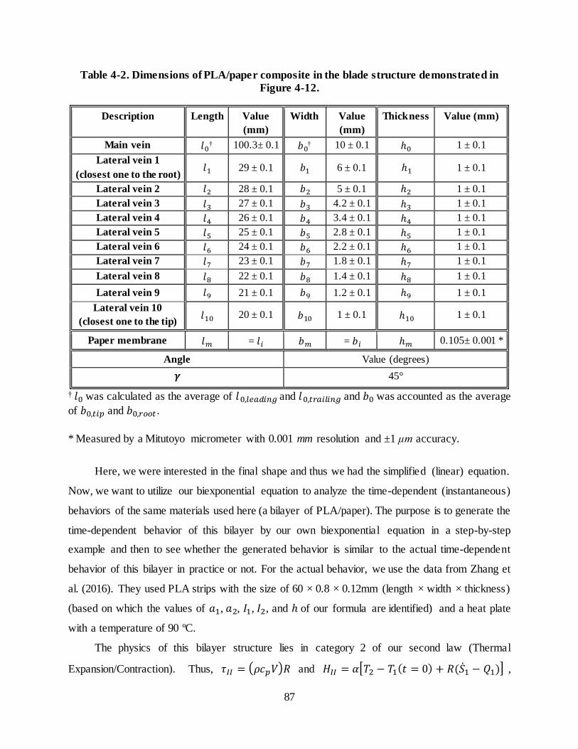
87

Table 4-2. Dimensions of PLA/paper composite in the blade structure demonstrated in

Figure 4-12.

Description Length Value

(mm)

Width Value

(mm)

Thickness Value (mm)

Main vein 𝑙0† 100.3± 0.1 𝑏0

† 10 ± 0.1 ℎ0 1 ± 0.1

Lateral vein 1

(closest one to the root) 𝑙1 29 ± 0.1 𝑏1 6 ± 0.1 ℎ1 1 ± 0.1

Lateral vein 2 𝑙2 28 ± 0.1 𝑏2 5 ± 0.1 ℎ2 1 ± 0.1

Lateral vein 3 𝑙3 27 ± 0.1 𝑏3 4.2 ± 0.1 ℎ3 1 ± 0.1

Lateral vein 4 𝑙4 26 ± 0.1 𝑏4 3.4 ± 0.1 ℎ4 1 ± 0.1

Lateral vein 5 𝑙5 25 ± 0.1 𝑏5 2.8 ± 0.1 ℎ5 1 ± 0.1

Lateral vein 6 𝑙6 24 ± 0.1 𝑏6 2.2 ± 0.1 ℎ6 1 ± 0.1

Lateral vein 7 𝑙7 23 ± 0.1 𝑏7 1.8 ± 0.1 ℎ7 1 ± 0.1

Lateral vein 8 𝑙8 22 ± 0.1 𝑏8 1.4 ± 0.1 ℎ8 1 ± 0.1

Lateral vein 9 𝑙9 21 ± 0.1 𝑏9 1.2 ± 0.1 ℎ9 1 ± 0.1

Lateral vein 10

(closest one to the tip) 𝑙10 20 ± 0.1 𝑏10 1 ± 0.1 ℎ10 1 ± 0.1

Paper membrane 𝑙𝑚 = 𝑙𝑖 𝑏𝑚 = 𝑏𝑖 ℎ𝑚 0.105± 0.001 *

Angle Value (degrees)

𝜸 45°

† 𝑙0 was calculated as the average of 𝑙0,𝑙𝑒𝑎𝑑𝑖𝑛𝑔 and 𝑙0,𝑡𝑟𝑎𝑖𝑙𝑖𝑛𝑔 and 𝑏0 was accounted as the average

of 𝑏0,𝑡𝑖𝑝 and 𝑏0,𝑟𝑜𝑜𝑡 .

* Measured by a Mitutoyo micrometer with 0.001 mm resolution and ±1 μm accuracy.

Here, we were interested in the final shape and thus we had the simplified (linear) equation.

Now, we want to utilize our biexponential equation to analyze the time-dependent (instantaneous)

behaviors of the same materials used here (a bilayer of PLA/paper). The purpose is to generate the

time-dependent behavior of this bilayer by our own biexponential equation in a step-by-step

example and then to see whether the generated behavior is similar to the actual time-dependent

behavior of this bilayer in practice or not. For the actual behavior, we use the data from Zhang et

al. (2016). They used PLA strips with the size of 60 × 0.8 × 0.12mm (length × width × thickness)

(based on which the values of 𝑎1, 𝑎2, 𝐼1, 𝐼2, and ℎ of our formula are identified) and a heat plate

with a temperature of 90 ºC.

The physics of this bilayer structure lies in category 2 of our second law (Thermal

Expansion/Contraction). Thus, 𝜏𝐼𝐼 = (𝜌𝑐𝑝𝑉)𝑅 and 𝐻𝐼𝐼 = 𝛼[𝑇2 − 𝑇1(𝑡 = 0) + 𝑅(��1 − 𝑄1)] ,

88

where 𝜌 = 1240 Kg

m3 (density of PLA is well-known), 𝑐𝑝 = 1800

J

Kg.K (heat capacity of PLA is

well-known). 𝑉 = 60 mm × 0.8 mm × 0.12 mm = 5.76× 10−9 m3 . The thermal resistance

of a rectangular slab is 𝑅 = 𝐿/𝐴𝑘, where 𝐿 is the length of the slab in the direction of heat flow

(and thus 𝐿 = 0.12 × 10−3 m), 𝐴 is the area of the slab perpendicular to the direction of heat flow

(and thus 𝐴 = 60 × 0.8 = 48 × 10−6 m2), and 𝑘 is thermal conductivity (𝑘 = 0.13𝑊

𝑚·𝐾 that is

well-known for PLA). Therefore, 𝜏𝐼𝐼 = 0.25 (s). The quantities ��1 and 𝑄1 can be assumed zero in

heat transfer, 𝑇1(𝑡 = 0) = 25 ºC, 𝑇2 = 90 ºC, and 𝛼 = 41 × 10−6 (1

𝐾) (this is the thermal

expansion coefficient of the active layer, PLA, which is well-known. The passive layer has 𝛼𝑚 =

0 (1

𝐾) as mentioned earlier, which is consistent with the fact that the passive layer is not usually

responsive under stimuli). Therefore, 𝐻𝐼𝐼 = 2.67 × 10−3 (unitless). 𝐸2 = 2 × 10

8 (𝑃𝑎)

(measured in our DMA test as discussed earlier). 𝐸1 = 5× 109 (𝑃𝑎) (this is Young s modulus of

the paper as noted earlier).

To find 𝐻𝐼 and 𝜏𝐼, we need the following discussion. PLA is a typical viscoelastic material.

For such a material, there is a famous model in solid mechanics as 𝐸′′ =𝐸𝜏𝜔

𝜏2𝜔2+1, where 𝜏 =

𝜂

𝐸, 𝜂

is viscosity, 𝐸′′ is loss modulus, 𝐸 (or equivalently written as 𝐸′) is Young s (storage) modulus,

𝜔 = 2𝜋𝑓 and 𝑓 is the frequency in DMA test. In a typical single-material shape memory polymer,

to enable the shape memory effect, the required force is applied externally. However, in a multi-

material having active and passive elements, the force is generated internally between the active

and passive materials. In this bilayer, we can assume that the passive layer (paper) has the role of

a mechanism that applies the required force to the active layer (PLA). Therefore, the above

equation that is used for a single-material shape memory polymer, can be used for the PLA in the

PLA/paper bilayer in this example. Thus, 𝜏𝐼 in our formula would be equivalent to 𝜏 in the above

formula. To find 𝜏𝐼, we can do the shear test by DMA machine to find the shear storage and loss

moduli (𝐺′ , 𝐺′′) and then viscosity, or we can re-write the above equation as 𝜏𝐼2 −

𝐸

2𝜋𝑓𝐸′′𝜏𝐼 +

1

𝜔2= 0 and solve it by knowing the involved parameters. The value of storage modulus has been

measured in our DMA test (Figure 4-31) as discussed earlier in the mathematical modeling. The

value of loss modulus (𝐸′′) has also been measured in DMA test. It is illustrated here in Figure

4-8. To find 𝜏𝐼 from the equation above, we need the ratio of storage and loss modulus. The value

89

of 𝑓 from the DMA section is 1 Hz. Therefore, the value of 𝜏𝐼 is obtained. Finally, the value of 𝐻𝐼

has already been measured in the literature (Zhang et al., 2015; 2016) for this example. Now, the

values of all parameters in our biexponential equation are present (Table 4-3).

The generated behavior is seen in Figure 4-9. This behavior impressively has the same trend

of real behavior reported in the literature (Zhang et al., 2016). However, some gaps happen

between theory and practice. One immediate reason is that we obtained the result for one strip,

while the real behavior is related to multiple strips (the number of strips is not clear in the related

study). The coupling effect between several strips is also the next important reason for the

difference. By the coupling effect, we mean that the behavior of a PLA/paper strip with width 𝑤

is not similar to the behavior of 𝑛 PLA strips each of which having a width of 𝑤/𝑛 printed on

paper with some spacing between PLA strips. Nevertheless, the general trend is nicely generated.

If we just change the value of one of 𝜏𝐼, 𝜏𝐼𝐼 , 𝐻𝐼, 𝐻𝐼𝐼, the trend is totally corrupted as seen in Figure

4-10. This implies that this step-by-step analysis of our formula led us to the appropriate values of

parameters. Any deviation from these values, cannot lead to the correct behavior (even through

the biexponential formula).

It should be noted that, in chapter 2, we presented three laws. Laws are different from

theories. Law is the starting point and reveals something that exists. By further analysis, laws can

lead to theories. Theories are much more complicated expressions. The step-by-step example

analyzed here can show the way for future theories in 4D printing that can be built based on the

proposed laws. These laws capture and show the big picture and future theories can delve into

more details to find some models for 𝜏𝐼, 𝜏𝐼𝐼 , 𝐻𝐼, 𝐻𝐼𝐼 of our biexponential formula.

90

Table 4-3. Values of parameters of our biexponential formula for a bilayer of PLA/paper

composite . Number 1 indicates the passive layer (paper) and number 2 indicates the active

layer (PLA).

Parameter Value (Unit)

𝑬𝟏 5× 109 (𝑃𝑎)

𝑬𝟐 2 × 108 (𝑃𝑎)

𝒂𝟏 0.105 (𝑚𝑚)

𝒂𝟐 0.12 (𝑚𝑚)

𝑰𝟏 7.72× 10−5 (𝑚𝑚4)

𝑰𝟐 1.15× 10−4 (𝑚𝑚4)

𝒉 0.225 (𝑚𝑚)

𝑯𝑰 0.0155 (unitless)

𝑯𝑰𝑰 2.67 × 10−3 (unitless)

𝝉𝑰 0.6 (s)

𝝉𝑰𝑰 0.25 (s)

Figure 4-8. The behavior of the loss modulus of the PLA from DMA test (with the same

conditions considered for storage modulus in Figure 4-31).

91

Figure 4-9. The generated behavior of our biexponential formula for one strip and the real

behavior for multiple strips from Zhang et al. (2016). The exact number of strips was not

given in that experimental study (Zhang et al., 2016).

0

50

100

150

200

250

0 5 10 15 20

An

gle

of

rota

tio

n (d

egr

ee

s)

Time (s)

Experiment (for multiple strips)

Theory (for one strip)

92

Figure 4-10. Any deviation from the generated parameters in the step-by-step example,

cannot give the correct behavior. The experimental data are from Zhang et al. (2016).

4.3 Fabrications and shape-shifting demonstrations

The wind turbine blade structures in Table 4-1 are fabricated by printing PLA filaments onto

a piece of paper, which resembles the structure of plant leaves. The CAD models were transformed

from STL format to G-code by Cura software and imported to the printer (LulzBot, TAZ 5). The

printer was run under the following condition: printing resolution was set to 100 microns; nozzle

temperature was adjusted to 205 ℃; bed temperature was considered as 60 ℃, and printing speed

was tuned to 50 mm/s (Figure 4-11). PLA is a shape memory polymer having a 𝑇𝑔 (glass transition

0

200

400

600

800

1000

1200

1400

1600

1800

0 5 10 15 20

An

gle

of

rota

tio

n (d

egr

ee

s)

Time (s)



0

100

200

300

400

500

600

700

800

0 5 10 15 20

An

gle

of

rota

tio

n (d

egr

ee

s)

Time (s)



93

temperature) of 60 ºC. After printing process, each structure was heated to 110 ºC and maintained

at that temperature for 10 min to reach the equilibrium. It was then cooled down to the room

temperature in the atmospheric condition, and the desired bend-twist coupling shape-shifting was

achieved.

Figure 4-11. Printer TAZ 5 test setup for printing the plant-leaf mimetic architectures.

4.3.1 Results and discussions

Here, we have six items. In the first four items, we analyze the technical advantages of the

proposed wind blade. In item 5, we discuss eco-friendly attributes of the proposed blade. In item

6, we discuss the unique advantages of the proposed blade compared to other blades capable of

BTC through passive methods.

4.3.1.1 Plant leaf-mimetic structure

As shown in Figure 4-11, the proposed structure mimics the pattern of the plant leaf. The

plant leaf-mimetic structure proposed in the literature remained mainly at the level of simulations

including geometry optimization. Its fabrication was challenging.

This is because, first, the vein network has a complex and subtle geometry and its fabrication

can hardly be achieved by the conventional manufacturing processes. In addition to the first-level

veins, there are second- and third-level veins (smaller branches) that support structural and

mechanical properties and can be explored in the future. Second, more difficulties are raised in

traditional manufacturing processes with the fabrication of complex geometries by using smart

94

materials such as shape memory polymers (Choong et al., 2017). This is resolved in this study by

4D printing process that is the convergence of additive manufacturing and smart materials (as well

as mathematics). This study demonstrates the plant leaf-mimetic wind blade structure in practice.

In addition, it has simultaneously other advantageous attributes. This feature of the proposed blade

is in favor of structure durability as discussed in the introduction.

4.3.1.2 Reversible bend-twist coupling shape-shifting

The architecture with an angle of 45° between the main and lateral veins had more twisting

in the tip than in the root, which was desirable. The angle of 90° had more twisting in the root than

the tip for both constant-width and varying-width cases, which was unsuitable. The angle of 65°

had similar twisting from tip to root for both constant-width and varying-width cases, which was

also unsuitable. Based on simulations, Liu et al. (2010; 2011) showed that the best fatigue life

happened in blades having angles of 45°-65° between their main and lateral veins. This is not only

coincident with the related angle of most natural plant leaves seen in the environment, but also

increasing the blade fatigue life remarkably (Liu et al., 2010; 2011).

Additionally, the blade structure with varying width that mimics more accurately the actual

pattern of plant leaf shows a better and more uniform twisting overall. The bend-twist coupling

shape-shifting behavior was reversible by re-heating. This feature of the proposed blade is in favor

of aero-elasticity (load reduction and energy gain) as discussed in the introduction. Figure 4-12

shows the structure for the desired bend-twist coupling shape-shifting, which has the angle of 45°,

1 mm thickness, and varying-width lateral veins.

Figure 4-12. (a) Originally printed flat blade without heat treatment (b) Bend-twist

coupling after heat treatment.

4.3.1.3 No need for electromechanical and moving parts

The structures can demonstrate the desired bend-twist coupling shape-shifting only by

providing the stimulus (heat), which removes the requirement of moving parts and traditional

electromechanical systems such as external sensors and actuators that are required in the active

a b

95

control. The necessity of the conventional sensor is eliminated by employing the smart (active)

material during the printing. The need for the conventional actuator is removed by printing the

active and passive materials in a special spatial arrangement based on mathematical modeling to

guide the mismatch-driven forces into the desired directions to provide the BTC shape-shifting.

This feature of the proposed blade is in favor of control simplicity.

4.3.1.4 Decoupled flexibility and adaptability

It should be emphasized that the flexibility is different from adaptability. An adaptive blade

can change its shape from shape one to shape two. However, shapes one and two can be either

rigid or flexible. In the literature, the bend-twist coupling (BTC) shape-shifting in wind turbines

is achieved either by using controllers (active method) or by utilizing the anisotropic mechanical

properties of a composite structure (passive method). The passive method is currently the focus of

the studies owing to its advantages (Lobitz et al., 1996; Veers et al., 1998; De Goeij et al., 1999;

Lobitz et al., 2001; Griffin, 2002; Veers & Lobitz, 2003; Bottasso et al., 2013; Nicholls-Lee et al.,

2013; Fedorov & Berggreen, 2014; Hayat & Ha, 2015; Zhou et al., 2015; Hayat et al., 2016;

Stäblein et al., 2017). However, the BTC through the existing passive methods has one big issue

that is flutter instability. This issue occurs because the blade needs to be flexible to demonstrate

the BTC under wind loads through the current passive methods. A more flexible blade has a higher

risk for flutter instability (Hayat et al., 2016; Bir & Jonkman, 2007; Politakis et al., 2008; Cognet

et al., 2017). We demonstrated a blade that could show the BTC without the need of flexibility

such that both the initial and deformed shapes could be as much rigid as needed. It would become

soft and flexible only during the shape-shifting process, when it is above the glass transition

temperature. It can be rigid during the usual operation. Its rigidity can be adjusted to any degree

that is desired depending on a specific application by changing the thickness of the smart material.

This feature of the proposed blade may solve the flutter instability and can be explored in a separate

study, quantitatively.

It should be noted that during the shape-shifting, the structure is not too flexible to cause a

failure under the external loads. In addition, the flexibility of PLA can be tuned depending on a

specific need by incorporating some additives into PLA or by suitable synthesis processes on pure

PLA (Mittal et al., 2015; Wang et al., 2018). However, the effect of external loads on the shape-

shifting angles in a specific application should be considered and incorporated in the mathematical

equations to have accurate predictions of shape-shifting behaviors.

96

In the proposed blade design, a thickness of 1 mm for the veins showed an adaptive blade,

in which both the flat and deformed shapes were rigid under the wind loads in the wind tunnel.

However, the blade with a thickness of 0.2 mm (and 0.4 mm) displayed adaptive blade with

flexible flat and deformed states.

The technical advantages of the developed wind blade in this study are summarized in Figure

4-13.

Figure 4-13. The technical advantages of the proposed wind turbine blade.

4.3.1.5 Eco-friendly attributes

To pave the ways for the future sustainable world, several advancements such as novel eco-

friendly wind turbines are needed in the near future (Figure 4-14). The eco-friendly attributes of

the proposed blade are:

1. Biodegradable materials: The smart material employed in the proposed blade is PLA,

which is biodegradable that can lead to eco-friendly wind turbines. PLA is a bio-based

polymer generated from natural resources such as corn and is one of the cheapest

biodegradable polymers to supersede petroleum-based plastics (Dong et al., 2014;

Mallegni et al., 2018). It is currently utilized in rigid bottles for beverage, yogurt and so on

(Mallegni et al., 2018) and has potential applications in many other industries such as

97

automotive (Dong et al., 2014). PLA is usually degraded by hydrolysis (Garlotta, 2001).

Recent industrial technologies could produce PLA with high molecular weights suitable

for structural applications with enough lifetime and no rapid hydrolysis (Avella et al., 2009).

An experiment showed that, in air, PLA begins to degrade at 300 ℃ (Sombatdee et al.,

2018). Nevertheless, depending on biodegradability needs in a specific application, the

biodegradability of PLA can be tuned through several ways such as coating with beeswax

to decrease water vapor permeability and biodegradability (Reis et al., 2018) or cold plasma

treatment to increase the biodegradability (Song et al., 2016).

2. Low mass: The low mass of the proposed blade is the next benefit. Blade mass

minimization is one of the four main objective functions engaged to optimize wind turbine

performance (Chehouri et al., 2015)

3. Low carbon emission: Ji & Chen (2016) analyzed the overall carbon footprint in the full

life cycle of a representative wind farm by considering construction, operation, and

dismantling phases. They showed that the most carbon emission was related to the

construction phase and in this phase, “smelting and pressing of metals” has the highest

share of carbon emissions. The proposed blade is not involved in such concern.

Figure 4-14. From purely rigid ancient wind turbines (such as Persian panemone (Dodge,

2006)) toward the future plant leaf-mimetic, smart, and eco-friendly wind turbines.

98

4.3.1.6 Comparison between the proposed blade and other blades capable of bend-twist

coupling through passive manners

The overall advantages of the proposed blade were discussed in the previous sections. Now,

the unique advantages of this blade compared with the existing blades capable of BTC through the

passive manners can be summarized as three main benefits. These are the plant leaf-mimetic

structure that improves the mechanical and structural properties, decoupled flexibility and

adaptability that may solve the flutter issue, and the eco-friendly features that may pave the way

for the future sustainable world. Additionally, the optimization of the proposed paradigm can be

studied in future investigation to explore the energy and power gains improvement.

4.4 Wind tunnel tests

Based on the above results, the blade structure with the angle of 45° between the main and

lateral veins, 1 mm thickness and varying-width lateral veins is selected for the following wind

tunnel test. Aerodynamics and performance of the originally printed flat blade and the final

deformed blade that has been exposed to the thermal stimulus, as shown in Figure 4-12(a) and (b),

are compared.

In this experiment, a wind tunnel was assembled by a fan (Model No. #122 “FC” HD Arr

9H, IAP Inc.), a direct current permanent magnet motor (Model C4D17FK10, LEESON Electric

Corporation), a manometer (Model No. 400-, Dwyer Instrument Inc.), and subminiature load cells

(Model 11 with tension/compression, Honeywell). The wind tunnel setup was connected to a PC

with LabVIEW software (version 2014, National Instruments) through an NI-cDAQ chassis. The

ambient temperature and pressure were 21.4 ± 0.1°C and 99.63 ± 0.05 kPa measured by a Wireless

Weather Forecaster (model TE688W, Meade Instruments) with temperature resolution of 0.1°C,

pressure resolution of 0.01 kPa, negligible temperature accuracy error, and pressure accuracy error

of 0.05 kPa.

The ambient temperature and pressure are for determining the density and viscosity of air.

Viscosity is used in Reynolds number calculations. Density is for calculating Reynolds number as

well as wind speed based on the Bernoulli equation. The drag and lift are measured by the

subminiature load cells that have ± 0.5% accuracy. The precision error of the lift and drag forces

is obtained from the LabVIEW program by considering a 95%-confidence-interval. The wind

speeds are calculated by using the pressure data from the manometer and the Bernoulli equation.

The manometer has 1 Pa resolution error, ± 2% accuracy error and the precision error obtained by

99

repeated measurements. These three types of errors (resolution, accuracy and precision errors) are

combined to determine the uncertainties and error bars. Figure 4-15 shows the wind tunnel test

setup.

Figure 4-15. Wind tunnel test setup.

4.4.1 Results and discussions

4.4.1.1 Calibration curves

The output of subminiature load cells of the wind tunnel is in mV/V. The wind tunnel load

cells need to be calibrated to find the conversion factor between the load cell output (in mV/V)

and the desirable drag and lift forces in Newton (N). To this end, we used several calibration

masses (10 g, 20 g, 50 g, 100 g, and 150 g) and one Correx tension gauge (model 1001681, 500 g

CNP KM) with an accuracy of ±0.01 × (maximum dial reading + actual test reading) and the

resolution error of 0.05 N. For a stationary object in the wind tunnel, the drag force is in the same

direction as the wind, while the lift force can be either upward or downward depending on the

shape of the object. Therefore, we consider only one horizontal direction for the drag force

calibration by using the Correx force gauge. However, we consider both the vertical directions for

the lift force by using the calibration masses for the downward force and Correx force gauge for

the upward force. The force gauge can be used to calibrate the downward lift as well, but the

calibration masses are used for this direction, as they are more accurate compared to the force

Test chamber

LabVIEW

program

Wind tunnel

motor controller

Force gauge and standard

weights for calibration

Dwyer manometer

Lift and drag

load cells

NI-cDAQ

chassis

100

gauge. The sample for the calibration is a rectangular cuboid Balsa wood with the dimensions (51

± 1 mm) × (51 ± 1 mm) × (102 ± 1 mm). The calibration curves are presented in Figure 4-16. The

horizontal and vertical error bars have been calculated by combining all the three types of errors

including resolution error (𝑒𝑟) , precision error (𝑒𝑝) , and accuracy error (𝑒𝑎) based on the

following equation:

𝑈𝑛𝑐𝑒𝑟𝑡𝑎𝑖𝑛𝑡𝑦 = ±√𝑒𝑟2 + 𝑒𝑝

2 + 𝑒𝑎2 (4-5)

A best-fit line was plotted for both the calibration curves and the slope of these curves was

the conversion factors. These conversion factors can be used for the test on the blades, in which

the raw data in mV/V are multiplied by these factors to yield the lift and drag forces in N. The

uncertainty in each of these conversion factors is twice the error in slope with 95%-confidence-

interval uncertainty. The error in slope can be obtained by the following formula (Heald, 1992) for

a line (𝑦 = 𝑎𝑥 + 𝑏) that is fitted to data,

𝑒𝑟𝑟𝑜𝑟 𝑜𝑓 𝑠𝑙𝑜𝑝𝑒 = 𝜎𝑎 = 𝑎√1𝑅2− 1

𝑁 −2

(4-6)

Where 𝑎 is the slope, 𝑅2 is the correlation factor and 𝑁 is the number of data points. The

conversion factors are obtained as 0.256 ± 0.017 for the drag force and 0.254 ± 0.004 for the lift

force. The vertical error bars for the downward lift (negative lift) are smaller than the upward lift

(positive lift). This is consistent with the assumption that the standard masses used for the

downward lift calibration have less uncertainty than the Correx force gauge.

101

Figure 4-16. (a) Drag load cell calibration, only for one horizontal direction. (b) Lift load

cell calibration, for both upward and downward vertical directions.

4.4.1.2 Aerodynamics of the flat blade versus deformed blade

The two flat and deformed blades (Figure 4-12) are tested in the wind tunnel chamber (Figure

4-17). The lift and drag forces at various speeds are measured based on the conversion coefficients

Drag (N) = 0.256Drag (mV/V) + 0.028

R² = 0.9983

Lift (N) = 0.254Lift (mV/V) - 0.019

R² = 0.9998

a

b

102

from the previous calibrations, and the results are shown in Figure 4-18. The speed values were

gained by using the Bernoulli equation and the pressure data from manometer. To convert the

pressure data from manometer to wind speed, the following simplified equation (Dwyer

Instruments Inc., 2010) derived from Bernoulli equation was used:

𝑉 = 1096.7√𝑃𝑉𝜌

(4-7)

Where, 𝑃𝑉 is the pressure measured by manometer in inch-of-water, 𝜌 is the air density in

𝑙𝑏/𝑓𝑡3 and 𝑉 is the wind speed in ft/min.

The resolution, accuracy and precision errors in forces gained from the load cells construct

the vertical error bars, while these three errors in wind speeds obtained from the manometer data

underpin the horizontal error bars in Figure 4-18. The sample is mounted to a sting installed inside

of the test chamber. The other end of the sting is attached to the load cells for force measurements

as shown in Figure 4-17. The lift and drag forces from the sting are measured as well, which is

then subtracted for determining the lift and drag forces due to the samples only. It should be noted

that for the vertical direction, along which the blades were mounted to the sting shown in Figure

4-17 (a), (b) and (c), the lift is in the downward direction (negative), and the results in Figure 4-18

illustrate the absolute values of the lift forces. If we install the blades upside down, the lift would

be upward.

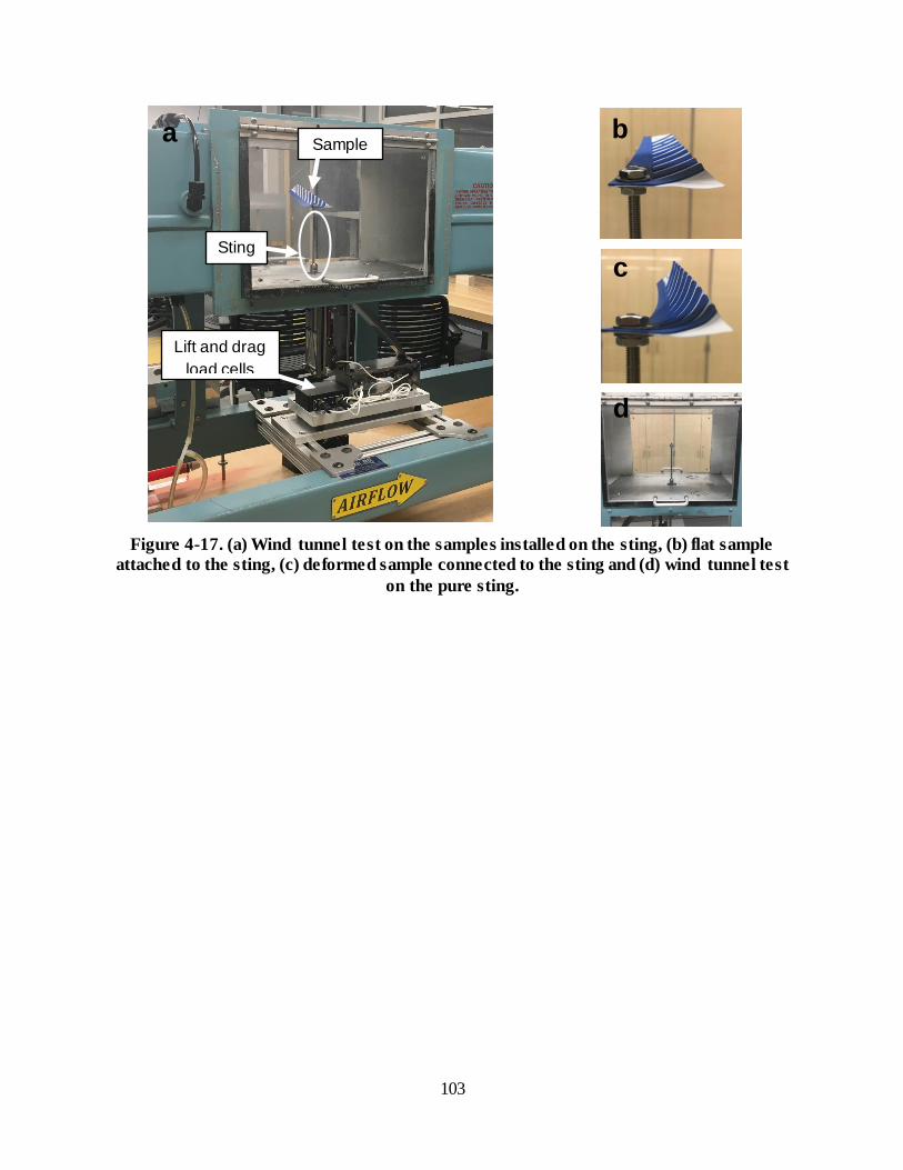
103

Figure 4-17. (a) Wind tunnel test on the samples installed on the sting, (b) flat sample

attached to the sting, (c) deformed sample connected to the sting and (d) wind tunnel test

on the pure sting.

a

Lift and drag

load cells

Sting

Sample a b

c

d

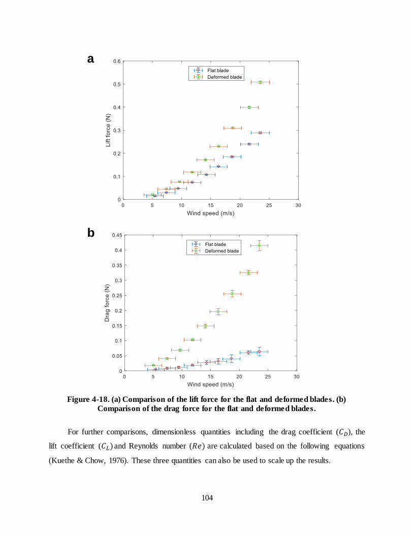
104

Figure 4-18. (a) Comparison of the lift force for the flat and deformed blades. (b)

Comparison of the drag force for the flat and deformed blades.

For further comparisons, dimensionless quantities including the drag coefficient (𝐶𝐷), the

lift coefficient (𝐶𝐿) and Reynolds number (𝑅𝑒) are calculated based on the following equations

(Kuethe & Chow, 1976). These three quantities can also be used to scale up the results.

b

a

105

𝐶𝐷 =𝐹𝐷

12𝜌𝑉2𝐴

(4-8)

𝐶𝐿 =𝐹𝐿

12𝜌𝑉2𝐴

(4-9)

𝑅𝑒 =𝜌𝑉𝐿

𝜇 (4-10)

Where 𝐹𝐷 , 𝐹𝐿 , 𝜌 , 𝑉 , 𝜇 , 𝐿 and 𝐴 are the drag force, lift force, air density, air speed, air

dynamic viscosity, characteristic length and the reference area of the sample, respectively. The

drag coefficients are calculated based on the frontal area of the samples and the lift coefficient s

are calculated based on the top area of the samples. The top and frontal areas of the deformed blade

are calculated based on a CAD reconstruction of the experimentally obtained blade, which is

explained in more details in the next section. Corresponding parameters for calculations of 𝐶𝐷 and

𝐶𝐿 are listed in Table 4-4 and the results are shown in Figure 4-19 (a) and (b). The error bars in

Figure 4-19 are calculated based on the sequential perturbation method by using equations (4-8),

(4-9), and (4-10) and the measurements of the lift force, drag force, and wind speed (Figure 4-18).

Table 4-4. Values of parameters for calculating 𝐂𝐃, 𝐂𝐋 and 𝐑𝐞.

Parameter (Symbol) Value (Unit)

Temperature (𝑻) 21.4 ± 0.1 (℃)

Pressure (𝑷) 99628 ± 50(𝑃𝑎)

Dynamic Viscosity (𝝁) 1.84E − 5 ± 0.00𝐸 − 5 (

𝑘𝑔

𝑚.𝑠)

Density (𝝆) 1.17 ± 0.00 (

𝑘𝑔

𝑚3)

Characteristic length (𝑳) 0.1± 0.0 (𝑚)

Deflected Frontal Area (𝑨𝑭,𝑫𝒆𝒇.) 0.0013 ± 0.0002 (𝑚2)

Deflected Top Area (𝑨𝑻,𝑫𝒆𝒇.) 0.0024 ± 0.0002 (𝑚2)

Flat Frontal Area (𝑨𝑭,𝑭𝒍𝒂𝒕) 0.00010 ± 0.00004 (𝑚2)

Flat Top Area (𝑨𝑻,𝑭𝒍𝒂𝒕) 0.0029 ± 0.0002 (𝑚2)

106

Figure 4-19. (a) Comparison of the lift coefficient for the flat and deformed blades. (b)

Comparison of the drag coefficient for the flat and deformed blades.

The 𝐶𝐷 and 𝐶𝐿 show that the deformed blade has a higher non-dimensional lift force and

lower non-dimensional drag force compared with the flat blade, which demonstrate the better

aerodynamics in the bend-twist coupled blade. It should be noted that based on the physics of the

problem, the pressure drag is of much greater magnitude and importance than the other types of

a

b

107

drag. Hence, in order to normalize the drag force, one can use the blade frontal area, from which

the dominant term of drag (pressure drag) originates (NASA Glen research center page, accessed

2018; Hedenstrom & Liechti, 2001). Due to larger frontal area of the deformed blade in

comparison to the flat blade, its drag coefficient is smaller than that of the flat one, although the

numerator of the drag coefficient (that is drag force) may increase itself. Hence, although Figure

4-18 (b) shows that the deformed blade has a higher drag force, but its drag coefficient is lower as

can be seen in Figure 4-19 (b).

4.4.1.3 Blockage ratio

Blockage ratio is the ratio of the cross-section of the sample that is normal to the flow

direction divided by the cross-section of the wind tunnel test section (test chamber) normal to the

flow direction. In this experiment, the test chamber cross-sectional area normal to the airflow was

203 ± 1mm by 203 ± 1mm. Consequently, the blockage ratio for the deformed blade, flat blade,

and the calibration rectangular cuboid sample are 3.2 ± 0.5 %, 0.2 ± 0.1 % and 6.3 ± 0.2 %,

respectively. According to the literature (Howell et al., 2010), the blockage ratio should be less

than about 7% to ensure that the flows around the samples are unaffected by the walls.

4.5 CFD simulations and performance analysis

In this section, CFD analyses are performed to study additional characteristics of the 4D-

printed blade that could not be investigated in wind tunnel tests. It should be mentioned that the

dimensions of the simulated blade are the same as the tested blade in wind tunnel. Advantages of

the proposed blade can be further revealed. First, the simulation is validated with available

experimental data. Performance study is then carried out for various conditions including different

wind speeds, rotational speeds, etc. The wind speed interval of approximately 5 to 24 m/s is

rational, which lays between cut-in and cut-off speeds for small-scale wind turbines due to their

intrinsically high rotational speeds (Drumheller et al., 2015; Wan et al., 2015).

In the wind tunnel test as well as performance calculations, the amounts of the top and frontal

areas are needed in order to calculate aerodynamic coefficients (especially lift and drag coefficients)

(NASA Glen research center page, accessed January 2018; Hedenstrom & Liechti, 2001). These

areas can be easily obtained in a CAD software as shown in Figure 4-20. The top and frontal areas

of the deformed blade are calculated of about 0.0024 ± 0.0002 (m2) and 0.0013 ± 0.0002 (m2),

respectively. The uncertainties in the top and frontal areas arise from the reconstruction of the

deformed blade in the software based on the measured (x, y, z) coordinates of some specific points

108

of the deformed blade. The main and lateral veins are not shown in this figure because only the

aerodynamic shape of the blade (bend-twist coupled form) due to the deflection of these smart

veins is important and the veins themselves have only structural roles.

Figure 4-20. The top, frontal and lateral projections of the deflected 4D-printed blade.

As a validation of CFD simulations method, lift and drag forces on the fixed (stationary)

deformed blade are compared between wind tunnel data and numerical results at different wind

speeds. These comparisons are shown in Figure 4-21 and Figure 4-22, respectively, where the

horizontal axis is the wind speed, the primary vertical axes are lift or drag forces exerted on the

blade, and the secondary vertical axis is the percentage of error of numerical results with respect

to corresponding experimental data. The errors are in 5% to 10% from lower wind speeds to higher

wind speeds. This implies that the CFD simulations are in good accuracy and valid in order to be

implemented for further investigations on the proposed blade.

109

Figure 4-21. Comparison of lift force on a fixed deformed blade as a function of wind speed

between results of the wind tunnel tests and CFD simulations.

Figure 4-22. Comparison of drag force on a fixed deformed blade as a function of wind

speed between results of the wind tunnel tests and CFD simulations.

After validation of the numerical results, the rotational speed of blade in a rotor disk at

different wind speeds is determined, which is also helpful for future design criteria. This value is

determined by two groups of opponent moments. One is the driving torque from the wind

110

generated due to lift force on the blade, and the others are the opposite moments, including the

friction from bearings and preventer torque from the generator. Here, no study is going to be done

on bearing and generator selection and hence, their effects can be neglected to obtain an upper

limit for ideal working conditions. The rotational speed of the rotor disk increases until the velocity

triangles of different sections of the rotor blade change in such a way that their resultant yields a

zero net lift force (driving torque). Therefore, in general, as the wind speed goes up, turbine rotor

disk rotational speed increases. This behavior is shown in Figure 4-23 for the proposed 4D-printed

blade in a rotor disk. The rotor disk is chosen to have 6 blades and a hub radius of 5 cm. 6-bladed

rotor disk will be shown to be optimum from a certain point of view in a few paragraphs later. The

value of the rotational speeds in Figure 4-23 can be implemented for the future structural design

of the wind turbine (bearings, spars, etc.).

Figure 4-23. The increment of deformed blade RPM as the wind blows in higher speeds.

One crucial performance parameter of a wind turbine blade is its generated torque (due to

lift) as a function of wind speed. In order to verify the advantages of the proposed 4D-printed blade

(with outer geometry same as the tested blade in wind tunnel), its generated lift force at different

wind speeds is provided in Figure 4-24. The result is compared with the flat (non-heated) blade at

an angle of attack (AOA) slightly less than the stall value. According to the simulations on the flat

blade at different angles of attack, the stall angle is about 12.6° at the Reynolds number of about

23000. Hence, in order to avoid flat blade stall at higher Reynolds numbers (higher wind speeds),

111

it has been simulated at an AOA of 12.4°. The lift forces in this figure are from conditions wherein

both the deflected and flat blades were stationary. The higher values of lift force at various wind

speeds in Figure 4-24 show the superiority of the deformed blade over the flat one, albeit the flat

blade has an AOA (12.4°) just before its stall AOA (12.6°). Physically, in the pre-stall region,

higher AOA of the blade will lead to higher lift generation. Through wind tunnel tests, we have

already observed that the deformed blade has more lift generation than the flat blade when both

have the same angles of attack equal zero at the root. Here, we captured an interesting point that

the deformed blade with zero AOA at the root even has more lift compared with the flat blade

almost having its maximum pre-stall AOA at the root.

Figure 4-24. Generated lift on deflected shape of the proposed 4D-printed blade and its flat

shape at different wind speeds.

In addition, the optimum number of deformed blades in a full rotor disk is determined. In

this regard, rotor disks with different numbers of blades (3, 4, 6, 8, 10 and 12) have been simulated

for sliced-periodic disks (1/3, 2/4, 2/6, 2/8, 2/10 and 2/12) at a fixed position. As an example, the

corresponding sliced-periodic domain with 2 out of 6 blades of a rotor disk is shown in Figure

4-25. The hub radius is 5 cm as specified before. Inlet boundary and the imaginary shaft are also

shown in this figure.

112

Figure 4-25. The sliced-periodic domain used for simulation of a rotor disk with 6 blades,

containing only a couple of those blades.

In the next step, the amount of generated torque is selected as the criterion for performance

evaluation. Due to different blockage ratios and interactive effects of adjacent blades, the drag and

lift forces and consequently, the generated torque per blade depends on the number of blades in a

rotor disk, as shown in Figure 4-26 for a wind speed of 9.4 m/s. The maximum torque per blade

occurs at a rotor disk with 6 deformed blades. The values of this curve depend on wind speed.

However, the optimum number of blades for generating the maximum torque per blade remains at

6 by varying the value of air stream velocity.

113

Figure 4-26. Variation of generated torque per blade as a function of the total number of

blades in a full rotor disk (at the wind speed of 9.4 m/s).

Some important performance parameters for wind turbine blade are generally studied with

certain theories like Blade Element Momentum (BEM). However, the BEM method can only

predict these parameters accurately for large-scale turbines (Tummala et al., 2016). Due to these

limitations, in this study, numerical simulation is employed. As one of the most important

performance parameters, the power coefficient is calculated using equations (4-11), (4-12) and

(4-13) and plotted as a function of tip speed ratio (TSR) in Figure 4-27. It should be noted that the

trend of variation of the power coefficient with TSR depends on the incidence angle (the angle

between the root's chord line and the rotor axis) of the rotor blades (Tummala et al., 2016).

𝑇𝑆𝑅 =𝑟𝑡𝑖𝑝 .𝜔

𝑉𝑤𝑖𝑛𝑑 (4-11)

𝐶𝑝 =𝑇.𝜔

12𝜌𝐴𝑉𝑤𝑖𝑛𝑑

3 (4-12)

𝐴 = 𝜋𝑟𝑡𝑖𝑝2 (4-13)

114

In the formulas above, 𝑟𝑡𝑖𝑝 is equal to 15 cm considering a hub radius of 5 cm for the blade

with 10 cm of span (length) and 𝜔 is rotational speed of the rotor disk. T is the generated torque

on the blade rotating with the corresponding rotational speed (𝜔) at wind velocity of 𝑉𝑤𝑖𝑛𝑑. 𝜌 is

air density equal to its value during wind tunnel tests (1.17 𝑘𝑔

𝑚3) and 𝐴 is area of a circle

encompassing the rotor disk. For each wind speed, different rotational speeds have been considered

for the rotor disk, which yields in different values of TSR. Having the amounts of the generated

torque on the blade for all the wind speed-RPM couples from CFD, variation of power coefficient

versus TSR is achievable. The ratio of the hub radius to the blade tip radius of the proposed blade

may seem too small in comparison to that of the large-scale turbines. However, it should be noted

that for small-scale (micro) wind turbines, this ratio becomes smaller and some examples of such

small values can be found in some references (Sedaghat et al., 2012; Kishore et al., 2013).

In real operations, by utilizing different generator and bearings, they may have different

friction coefficients. The rotor disk would then be subjected to different amounts of opponent

moments. Therefore, at a certain wind speed, the rotor can have different rotational speeds and

consequently different TSRs depending on the utilized generator and bearings, which then change

the value of the power coefficients, accordingly. In this regard, Figure 4-27 compares the

relationship between the TSR and the power coefficient at different wind speeds for a rotor disk

with 6 deformed blades. It can be observed that the TSR value that maximizes the power

coefficient is independent of wind speed. Not only the maxima, but also the entire curve of power

factor versus TSR is independent of wind speed (Tummala et al., 2016). Figure 4-27 indicates

these independencies very well. Using the proposed 4D-printed blade, the maximum power

coefficient occurs at the TSR of about 0.6.

115

Figure 4-27. Performance curve of the 6-bladed rotor disk power coefficient vs. tip speed

ratio in five different wind speeds.

In addition to the above outcomes in CFD part, some qualitative analyses on numerical

results are provided. Figure 4-28 shows velocity contour lines at four different sections of the

deformed blade when it is rotating with an induced rotational speed of about 580 rpm due to the

wind speed of 9.4 m/s. Except a tiny partial flow separation occurs at the root of the blade, the

flow is fully attached to the blade surface especially near the tip (no tip stall is observed), which

has a more important effect on the aerodynamic performances compared with the root (Wetzel,

2005).

116

Figure 4-28. Velocity contours in 4 different chord-wise cross sections along the blade span

(0.01, 0.3, 0.6 and 0.9 of span).

Figure 4-29 and Figure 4-30 show the air streamlines and static pressure contours at those

four chord-wise sections at the same wind conditions, respectively. These reaffirm the good quality

of the airflow around the blade. Almost no flow separation exists around the blade, and the pressure

distributions are favorable (there is almost no reverse flow on the blade surface). A tiny partial

flow separation occurs at the root of the blade, which is due to a relatively high local angle of

attack. This arises from some structural constraints, which can be explained as follows: The blade

is subjected to a couple of perpendicular moments due to lift and drag forces. The moment from

the drag force is usually more crucial because the blade may not have any rotational motion in the

direction of drag force. Indeed, the maximum bending moment occurs at the root. The cross-

section of the root should, therefore, have a large Izz in order to withstand the moment exerted by

the drag force, which can be achieved by aligning of the chord of root parallel to the air stream.

This causes a relatively high local angle of attack at the root of the blade. However, the small

amount of flow separation at this region can have no considerable effect on the blade performance.

117

Figure 4-29. Air streamlines passing around the stationary 4D-printed blade in four

different chord-wise cross sections along the blade span. (a) 0.01, (b) 0.3, (c) 0.6 and (d) 0.9

of span.

118

Figure 4-30. Static pressure (gauge) contours in 4 different chord-wise cross sections along

the blade span. (a) 0.01, (b) 0.3, (c) 0.6 and (d) 0.9 of span.

In the CFD part of the present study, a novel 4D-printed blade is compared to a simple flat

plate. In other words, the 4D-printed deformed blade is considered as a thin flat plate which is

deformed and curved. Therefore, the whole present analysis is about the improvement gained by

4D deformation of a thin plate inspired by leaf structure, so the performance is also compared with

a flat plate as presented in CFD part. The present cross-section may be the camber of any arbitrary

119

airfoil section profile for upper and lower surfaces. In fact, there is a high potential for future

investigations to improve both aerodynamic and structural performance of the leaf-mimetic 4D-

printed blades with airfoil cross-sections. Apart from aerodynamic performance, structural

characteristics (strength to weight ratio, etc.), manufacturing expenses, and attainability of

desirable shape deformation are other concepts, which must be investigated in separate studies.

Along with the CFD simulations and in order to compare the power range quantitatively, a

6-bladed commercially-used small-scaled wind turbine with a rotor disk diameter of 91 cm is

considered (Marlec Eng. Co. Ltd.). Referring to the performance curves, its power production

varies from almost 2 to 222 Watts in the operating range of wind speed from 3 to 15 m/s. The

present 4D-printed blade, with 5 cm hub radius and blade length of 10 cm, has a rotor disk with a

diameter of 30 cm. According to a simple scaling law (Amano & Sundén 2014; Manwell et al.,

2010), the power of the turbine is proportional to the square of the diameter of its rotor disk. This

proportionality is also examined numerically in the present study. Consequently, after scaling the

4D-printed rotor disk diameter from 30 to 90 cm, its power (obtained from present CFD results)

lies between 2.2 to 174 Watts for wind speeds of 5.5 to 23.5 m/s. A result which is comparable to

that of commercially-used small-scaled turbines with conventional blades.

The main purpose of these simulations, however, is to evaluate the performance of the 4D-

printed blade in more details and complement some limitations of experimental tests and analytical

solutions. In fact, these analyses serve to implement the proposed design and fabrication paradigm

in this study for advanced 4D-printed wind turbine blades in future works.

4.6 Dynamic Mechanical Analysis (DMA) tests

One of the critical material properties that needs to be determined in the mathematical model

in equation (4-3) is the elastic (storage) modulus of the polymer above the glass transition

temperature 𝑇𝑔 . The shape memory polymers have a temperature-dependent elastic modulus,

especially around the 𝑇𝑔 and it can be measured from Dynamic Mechanical Analysis (DMA) test.

Some of the studies in the literature used the results of the DMA test on molded structures

for analyzing the deformation behavior in 4D printed structures, which is conceivably inaccurate.

To verify this statement, DMA tests were performed on a treated printed PLA.

The test was performed in the tensile mode with a DMA machine under the following

condition: the strain oscillation had a frequency of 1 Hz with a maximum amplitude of 0.01%. The

120

temperature ranged from 40 to 130 ℃ at an increasing rate of 2 ℃/𝑚𝑖𝑛. A static preload of about

0.1𝑔 (0.001𝑁) was considered to maintain the specimen straight during the whole experiment as

was done in some of the previous studies (Wu et al. 2016).

It is seen that some researchers use the materials properties of molded or annealed structures

to model the behavior of their 4D printed structures. Here, we measure the desired property of our

4D printed structure (Figure 4-31) and observe that the manufacturing process affects materials

properties. It should be noted that our smart blade will have multiple shape-shifting behaviors

(cycles) rather than only one cycle. Therefore, we consider this point and measure the desired

property of a printed structure that has already gone one shape-shifting cycle. We just call this

structure as “treated printed” structure to distinguish it from “just printed” structure. After the first

shape-shifting cycle, the structure would behave as a "treated printed" structure for the rest of the

shape-shifting cycles, rather than the "just printed" structure. Therefore, the "treated printed"

structure is closer to reality than the "just printed" structure.

Comparing the measured results in Figure 4-31 with the properties of a molded PLA from

Cock et al. (2013) in Figure 4-32, the elastic modulus shows an entirely different behavior as a

function of temperature. The elastic modulus for the molded PLA has a local minimum value and

then increases after the glass transition temperature. On the other hand, the elastic modulus in a

treated printed PLA uniformly decreases as the temperature increases. This shows that the

manufacturing process directly influences these material properties not only on their absolute

values (especially around the 𝑇𝑔) but also on their general trends. This difference can lead to

tremendously different results in predicting the behavior of the 4D printed structures. Based on

Figure 4-31, the elastic modulus well above 𝑇𝑔 of the treated printed PLA is 2 × 108 𝑃𝑎, which

was used in the mathematical modeling. In contrary, Figure 4-32 shows that the value of the elastic

modulus for molded PLA well above 𝑇𝑔 is around 5× 107 𝑃𝑎.

Therefore, for accurate mathematical modeling and prediction of the shape-shifting behavior

over time, the actual material properties of the 4D printed structure should be used.

121

Figure 4-31. The behavior of the elastic (storage) modulus of the “treated printed” PLA

from DMA test.

Figure 4-32. The behavior of the elastic (storage) modulus of the “molded” and “annealed”

PLA from DMA test (Cock et al., 2013).

4.7 Discussions

4.7.1 Mechanisms for applying stimulus

In this study, we utilized a hot plate (CIMAREC, model SP131325) to provide heat in the

lab. The mechanisms that can supply heat in real operations can be studied, separately. For example,

122

a connection can be made between the environmental temperature and the desired shape changes,

instantaneously; or some hot wires can be embedded through the smart parts (PLA) of the blade

to apply heat locally. This heat can be provided by electricity or even by a mechanism that

incorporates the free energy of sunlight. In addition, photo-responsive smart materials can be used

in our design rather than the current heat-responsive smart material. In this case, the desired shape

can be achieved directly by light (i.e., photochemical mechanism) without reliance on heat and

temperature change (as seen in photothermal mechanism).

The frequency of the shape-shifting should also be considered in a specific application.

According to the Probability Density Function (PDF) and Cumulative Frequency (CF) of wind

speed and also wind rose graph of its direction in the region of installation site (Chen et al., 2016),

the materials compositions and layers directions can be set in the printing process. Then, depending

on these features and by dividing the wind speed range into some intervals, it can be determined

for the blade to shift its shape at certain wind speed and direction milestones. The required energy

for blade deflection is then dependent on the materials and structural characteristics of the blade ,

as well as wind intensity (speed) and direction. One main parameter that determines the amount of

the required heat is the glass transition temperature (𝑇𝑔) of the smart material that can be tuned by

some additives, blends, and even using some other types of smart materials. However, one of the

ultimate goals of 4D printing is using random free energy to provide non-random structures and

shape-shifting behaviors (Tibbits, 2013). It should be also noted that if the number of shape-

shifting is too many, then the 4D printed structure may not be able to totally recover its initial and

final shapes and this fact should be considered and monitored (Momeni et al., 2016).

The next consideration is related to seasonal variations in temperature that cause the blade

surface temperature to vary. The smart material used here has a glass transition temperature (𝑇𝑔)

of about +60 ℃, above which the shape-shifting occurs. Therefore, at any temperature below this

point, there is no unwanted shape-shifting. By the way, the 𝑇𝑔 can be decreased or increased as

discussed above.

4.7.2 Small-scale and large-scale applications

Here, we demonstrated the proof-of-concept of a new blade followed by wind tunnel tests

and performance analysis. The proposed paradigm can be explored for both small-scale and large-

scale applications. The three unique advantages of the proposed blade compared to the existing

123

blades capable of BTC through the passive methods (discussed in section 3.1.6), would be present

in both the small and large scales. In addition, the energy gain can be studied by optimizing the

proposed blade from various perspectives. It should be noted that, for large-scale applications, the

widths of main and lateral veins will increase. Thus, to avoid unwanted shape-shifting along the

width of a vein, the smart material should be printed as several small-width strips with some

spacing between strips, rather than a continuous large-width vein. Moreover, for the large-scale

wind turbines, the mechanical properties of the materials should be considered as the following.

4.7.3 Materials considerations

First of all, composite materials have been recognized as the best materials for wind blades

(compared to metals (primarily aluminum) and wood) (El Alaoui et al., 2016; Mishnaevsky et al.,

2017; Swolfs, 2017; Sutherland, 1999; Brøndsted et al., 2005; Jespersen & Mikkelsen, 2017; Dai

& Mishnaevsky, 2014). Moreover, if green composites (Dicker et al., 2014; Schledjewski et al.,

2017; Murdani et al., 2017) are used, then it will be eco-friendlier. For composite materials, fiber

and matrix should be analyzed separately. For matrix portion, two types of materials are usually

used; thermosets and thermoplastics. Compared to thermosets, thermoplastics are recyclable and

have higher fracture toughness, as well as larger elongation at fracture. Nevertheless,

thermoplastics have more difficult manufacturing processes due to their higher viscosity and larger

processing temperature compared to thermosets (Mishnaevsky et al., 2017). However, this

difficulty can be resolved by additive manufacturing. Here, we used PLA that is a biodegradable

thermoplastic. It can be reinforced by carbon fibers. PLA-carbon fiber blends are commercially

available for additive manufacturing. In addition, natural fibers such as Bamboo have been

reported as good alternatives to glass and carbon fibers for both the small- and large-scale wind

turbines (Mishnaevsky et al., 2017; Holmes et al., 2009; Pozo Morales et al., 2017). Nevertheless,

research on green composites suitable for large-scale wind turbine blades is ongoing.

4.7.4 Other plant-mimetic approaches useful for wind turbines

There was a different plant-mimetic approach for wind turbines, where the researchers (Loth

et al., 2017; Ichter et al., 2016; Noyes et al., 2018) were inspired by downstream bending of the

palm tree trunk in high winds leading to load reduction. In their design, the blades had the same

conventional structures (rather than leaf structure). However, they had a segmented structure close

to their rotor hub and could bend from that part, in the direction of the wind, similar to the palm

124

tree (and in contrast to the oak tree). This leads to load reduction and is suitable for extreme-scale

wind turbines (Loth et al., 2017; Ichter et al., 2016; Noyes et al., 2018). This approach can be

combined with our proposed blade mimicking the leaf vein network.

4.8 Conclusions

A new paradigm for the design and fabrication of the wind turbine blades has been

demonstrated by the 4D printing process. This can integrate several advantageous attributes into

one structure, simultaneously. Other materials can be incorporated. The results can be scaled up,

and the methodology can be adjusted and customized to a particular need. We demonstrated a plant

leaf-mimetic wind turbine blade in practice that is capable of reversible bend-twist coupling

behavior. This blade does not rely on traditional electromechanical systems, moving parts, sensors

and actuators. We have also separated the adaptability and flexibility concepts in wind turbine

blades and demonstrated this difference in practice. This may solve the flutter issue seen in blades

capable of BTC through passive methods. The proposed multi-functional blade can finally lead to

eco-friendly wind turbines. Our blade only relies on heat to show its shape memory effect, in

contrast to the usual shape memory materials that need both the heat (thermal part) and force

(mechanical part) to achieve the shape memory effect. This is because we combined active and

passive materials and designed their arrangement so that their mismatch-driven force serves as the

required mechanical force in the required direction. Finally, it should be noted that certain

materials properties of 4D printed structures, for example, the elastic (storage) modulus are

different from those of the molded/annealed structures. The actual materials properties of “4D

printed” structures should be applied in the corresponding mathematical models for predicting the

shape-shifting behaviors over time.

125

CHAPTER 5

NATURE-INSPIRED SMART SOLAR CONCENTRATORS BY

4D PRINTING

Currently, solar concentrators, whether in solar PV or solar thermal applications are designed

and utilized as a fixed shape such as elliptic, parabolic, V-shape, hyperbolic, and multi-stage forms.

Here, we are inspired by diurnal and nocturnal flowers and their differences and propose a smart

solar concentrator that can increase the overall light collection efficiency by more than 25%

compared with its non-smart counterparts. We introduce the concept of smart solar concentrators

inspired by nature and enabled by 4D printing and illustrate its necessity and advantages. We found

that most of the diurnal flowers have parabolic and most of the nocturnal flowers have hyperbolic

petals. Our proposed multi-functional concentrator has a parabolic shape for a portion of the day

that parabola dominates all the other shapes in terms of the optical efficiency, then it can reversibly

change its shape to hyperbola for another portion of the day that the hyperbola beats all the other

geometries. By using this design, the optical efficiency trend will move from peak-and-valley form

toward constant-at-peak format, resulting in overall efficiency improvement. The proposed

biomimetic structure is an example of smart origami. It is simple and low-mass. It demonstrates

the desired shape-shifting without reliance on cumbersome and expensive electromechanical

systems.5

5 This chapter is based on our journal article published in Renewable Energy 122 (2018), entitled “Nature-inspired

smart solar concentrators by 4D printing”, by Farhang Momeni and Jun Ni.

126

5.1 Introduction

Both the solar PV and solar thermal modules can have three main elements, a receiver

(mandatory), a concentrator (optional) and a tracking mechanism (optional). The primary reason

for using concentrators is to converge the sunlight and obtain the same efficiency by using less

solar cell materials in solar PV applications (Parida et al., 2011) and increase the receiver

temperature in solar thermal applications (Tian & Zhao, 2013). Currently, the solar concentrators

are designed as a fixed shape, and most of the existing solar concentrators are parabolic. Ellipt ic,

V-trough, and hyperbolic concentrators have been studied in few specific cases, and the parabolic

concentrators have been recognized as a suitable form for general purposes and usual operations

(Madala & Boehm, 2017; Khamooshi et al., 2014; Ghasemi & Ranjbar, 2017; Marefati et al., 2018;

Kasaeian et al., 2018; Bellos & Tzivanidis, 2017; Rabl, 1976; Khakrah et al., 2017).

On the other side, the reason for using the tracking mechanism is to keep perpendicular

sunlight incidence by tracking the apparent motion of the sun (Apostoleris et al., 2016). However,

the current tracking mechanisms are heavy, large, and expensive (due to the installation, operation,

auxiliary energy, and maintenance costs) (Madala & Boehm, 2017; Apostoleris et al., 2016). These

factors cause hurdles for the commercialization of concentrating photovoltaic (CPV) systems

(Apostoleris et al., 2016). This issue is going to be solved through several ways such as integrated-

tracking systems (Apostoleris et al., 2016; Duerr et al., 2011; Lamoureux et al., 2015) and/or

proposing simple, lower-mass and cheap tracking mechanisms by novel solutions, such as kirigami

technique (Lamoureux et al., 2015), and so on. Kirigami (‘kiru’: cut; ‘kami’: paper) and origami

(‘ori’: fold) can provide novel solutions for engineering applications by combing mathematics and

art (Blees et al., 2015; Rafsanjani & Bertoldi, 2017; Wang-Iverson et al., 2016; Ge et al., 2014).

By 4D printing, smart origami (Ge et al., 2014) and kirigami are achievable, in which the shape is

evolved by intelligence rather than mechanically-driven alterations by pure pushing and pulling.

Optical efficiency is one of the primary efficiencies in solar PV and solar thermal

applications, and in some cases, the overall efficiency of concentrating photovoltaic/therma l

(CPVT) collectors is limited by optical efficiency (Karathanassis et al., 2017; Daneshazarian et al.,

2018). This means that, in these cases improving factors other than optical efficiency, cannot give

a net improvement in the overall efficiency until this bottleneck (optical efficiency) is improved.

In optical efficiency analysis, ray-tracing simulation is a useful technique for the design, analysis,

and optimization of solar concentrators (Riveros-Rosas et al., 2011), especially by using TracePro

127

software (TracePro User’s Manual, 2017) that has attracted a growing level of attention (Wang et

al., 2017).

The design, analysis, and optimization of the four concentrators above have been explored

in several studies by numerical, experimental, and analytical approaches (Zhang et al., 2017; Tina

& Scandura, 2012; Ali et al., 2013; Tang & Wang, 2013; Sellami et al., 2012; Al-Shohani et al.,

2016; Mohsenzadeh & Shafii, 2017; Chaves, 2015; Gorjian et al., 2014). Here, we show the

necessity and advantages of a smart solar concentrator that has the desired reversible shape-shifting

in one specific case. We demonstrate the proof-of-concept for a low concentration (Amanlou et

al., 2016), one-stage, and compound concentrator. However, 4D printed solar concentrators can

be further analyzed in all the four shapes, in simple or compound, one- or multi-stage concentrators,

in the low, medium, or high concentration systems, in the solar PV or solar thermal applications,

etc. Moreover, it can be considered in various optimizations schemes.

Natural living things have evolved, self-corrected, self-adapted, and self-optimized to the

environmental conditions over a long time. Nature usually accomplishes a function with the least

amount of energy. Hence, biomimetic approaches can provide one of the most efficient, and most

robust solutions for human-made systems (Li et al., 2013; Vincent, 2006; Speck et al., 2017). Here,

we show how a biomimetic inspiration paves the way for a more efficient solar energy utilizat ion.

5.2 Design concept

There are three types of flowers. Some flowers are always open, some of them open in the

morning and close in the afternoon that is named diurnal flowers, and some others open in the

afternoon and close in the next morning that is called nocturnal flowers. The diurnal and nocturnal

flowers open and close for several reasons such as pollination and the type of pollinators (some

pollinators are night-flying, and some are day-flying), avoiding unwanted attention from other

harmful insects whether during the day or night, managing the internal temperature & humidity,

metabolism, etc. Nevertheless, one of the main growing requirements of both the diurnal and

nocturnal flowers is capturing as much sunlight as possible. However, the interesting point is that

the total performance (fruit or seed set) of these two categories are comparable in many cases

(Young, 2002; van Doorn & van Meeteren, 2003; ProFlowers, 2011; UCSB ScienceLine, accessed

2017; Shamoon, accessed 2017; Carter, accessed 2017; Avid, accessed 2017; Palermo, 2013;

Villazon, 2009). Therefore, we can say that there should be some competitive advantages in

nocturnal flowers that can yield the same performance, albeit they receive only the inclined portion

128

of the sunlight of a day and are closed around noon. We propose one competitive advantage,

demonstrate an impressive result based on this inspiration, utilize it in our smart solar concentrator

design, and show the efficiency gain.

We organize several popular nocturnal and diurnal flowers in Figure 5-1. A fascinating result

can be captured by analyzing the geometries of these two categories. The diurnal flowers have

mainly parabolic petals, while the nocturnal flowers have mainly hyperbolic (trumpet-shaped)

petals.

129

Figure 5-1. Comparing the configurations of petals in diurnal and nocturnal flowers.

Category (a) shows some popular nocturnal flowers . They are closed around noon and are

open far from noon. Category (b) illustrates some popular diurnal flowers. They are open

around noon and are closed far from noon (Palermo, 2013; Villazon, 2009; Taylor, 2017;

Wikipedia. Mirabilis jalapa, accessed 2017; Waluyo, 2015; Wikipedia. Nicotiana tabacum,

accessed 2017; Taylor, 2017; Wooden Shoe Tulip Farm, accessed 2017; Gardenia, accessed

2017).

Four o'clock (Mirabilis jalapa)Datura Angel's Trumpet (Brugmansia)

Moonflower Nicotiana Night-Blooming Jasmine

Tulip Crocus Poppy

a

b

130

Before we proceed to simulations, we discuss the reflectivity of the flowers petals. The

flowers petals have a combination of specular (mirror-like) and diffuse reflections (Moyroud et

al., 2017; Grant, 1987; Vogelmann, 1993; Hohmann-Marriott, 2014; Barthlott et al., 2017;

McClendon, 1984; Wehner & Bernard, 1993; Xie et al., 2017; Foster et al., 2014; Fritz et al., 2017).

The specular reflection generally results from the air-petal interface (Moyroud et al., 2017; Grant,

1987; Vogelmann, 1993). More interestingly, in some flowers such as Buttercup (Ranunculus

species), the specular reflection totally dominates the diffuse one, and the flowers petals, perfectly

reflect the sunlight toward the reproductive organs (van der Kooi et al., 2017) (Figure 5-2). The

highly specular reflection in Ranunculus is due to an incredibly smooth epidermal layer (van der

Kooi et al., 2017; Kooi et al., 2014; Parkin, 1928), and the presence of an air layer beneath the

epidermal layer (i.e., between the epidermal and starch layers) (Vignolini et al., 2011; van der Kooi

et al., 2017). The highly specular reflection has been reported in some other flowers (such as

Gorteria diffusa) that helps the pollination (Ellis & Johnson, 2010; Vignolini et al., 2012). Even,

metallic-mirror like surfaces were found in the mirror orchid Ophrys speculum (Barthlott et al.,

2017). The extremely specular reflection in the mirror orchid is due to an unusually smooth cuticle

layer (ultrastructure) resided on top of a very flat epidermal layer (Vignolini et al., 2012).

Figure 5-2. The specular reflection in flowers` petals. The flower photo of this figure was

taken by Dekker (accessed 2017).

5.3 Simulation

Now let s analyze these two geometries observed in the nocturnal and diurnal flowers

(hyperbola and parabola), by a ray tracing simulation software, TracePro. The general concepts

and procedures of ray tracing simulation by TracePro are shown in Figure 5-3. In Figure 5-3, θ is

θ r

θ i

=(Incidence angle) (Reflection angle)θ i θ r

Specular reflection

Reproductive

organs

131

the solar incidence angle. Light is beam and monochromatic with an average wavelength of 0.5461

µm (green color light). Concentrators have about 95% specular reflectance (standard mirror), and

the receiver is a perfect absorber (blackbody). Figure 5-3 also shows the irradiance maps of the

receiver surface that indicate the pattern and amount of absorbed flux. Both the black-white and

color maps show the absorbed flux by the receiver that is equal to the incident flux on the receiver,

as the reflected flux is zero for the perfect absorber. The color map is for better realization, and

further illustrates the incoming rays, concentrators, and receiver.

At this point, rather than comparing only parabola and hyperbola, we follow a recent work

(Madala & Boehm, 2016) and similarly consider all of the four shapes, elliptic, parabolic, V-shape,

and hyperbolic concentrators. The results are illustrated in Figure 5-4.

In Figure 5-4 the heights (H) and (geometric) concentration ratios (CR) of the four shapes

are the same, and each data point shows one particular simulation that illustrates the optical

efficiency at a specific irradiance angle. This figure implies two main points. First, we can find

that why most of the diurnal flowers have parabolic shape and most of the nocturnal flowers have

the hyperbolic shape as one reason. It shows that the parabolic shape is better in terms of optical

efficiency for perpendicular irradiance angles around noon and the hyperbolic shape is better for

inclined angles far from noon. Second, it can be understood that why most of the existing studies

worked on parabolic concentrators. They try to capture the perpendicular irradiations around noon,

as much as possible. In addition, it should be noted that the parabolic concentrator has easier

fabrication through the conventional manufacturing processes compared with the hyperbolic

counterpart.

Now, we propose 4D printed smart solar concentrators, which specifically in our case, can

be parabolic as long as parabola beats all other shapes in terms of optical efficiency and can

reversibly change its shape to hyperbola for another portion of the day that hyperbola has the best

performance among all the four shapes. To show the gain, let s consider three different scenarios

(cases) as seen in Figure 5-5. In this figure, we consider the overall (average) optical efficiency

(i.e., considering all irradiance angles) of a day for three cases. CPC and CHC stand for the

compound parabolic concentrator, and compound hyperbolic concentrator, respectively. Case 1

has a non-smart (static) parabolic concentrator for the whole day. Case 2 has a non-smart

hyperbolic concentrator for the entire day. However, case 3 has a 4D printed smart concentrator

that is parabolic for a portion of the day (i.e., between the two intersection points in Figure 5-4)

132

and can change to hyperbola for another portion of the day (i.e., outside of the intersection points).

The overall efficiencies of these three cases have been calculated based on Figure 5-4 by

considering all the irradiance angles. The overall efficiency of case 3 was obtained by considering

the efficiency of the CPC between the two intersection points, and the efficiency of the CHC

outside of the intersection points. It is observed that case 3 improves the overall optical efficiency

by more than 25% compared to cases 1 and 2. By further optimizations of concentrators, this gain

can be enhanced as well. It should be noted that the equality of the overall efficiencies of the CPC

and CHC is accidental. For example, if we change the present geometry of the CHC (in Figure 5-4

and Figure 5-5) and keep the same geometry for the CPC, then their overall efficiencies would

become different.

Figure 5-3. Concepts and procedures of Ray tracing simulations and optical analysis using

TracePro.

Irradiation

Source (Light is

beam and

monochromatic)

Concentrator

(Standard Mirror with

94.87% Specular

Reflectance)

Perfect Absorber

(Blackbody)

Morning (θ<0) Afternoon (θ>0)Noon (θ=0)

Aperture

area

Receiver

area

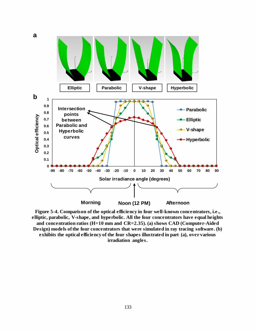
133

Figure 5-4. Comparison of the optical efficiency in four well-known concentrators, i.e.,

elliptic, parabolic, V-shape, and hyperbolic. All the four concentrators have equal heights

and concentration ratios (H=10 mm and CR=2.35). (a) shows CAD (Computer-Aided

Design) models of the four concentrators that were simulated in ray tracing software. (b)

exhibits the optical efficiency of the four shapes illustrated in part (a), over various

irradiation angles.

Elliptic Parabolic V-shape Hyperbolic

0

0.1

0.2

0.3

0.4

0.5

0.6

0.7

0.8

0.9

1

-90 -80 -70 -60 -50 -40 -30 -20 -10 0 10 20 30 40 50 60 70 80 90

Op

tic

al e

ffic

ien

cy

Solar irradiance angle (degrees)

Parabolic

Elliptic

V-shape

Hyperbolic

Intersection

points

between Parabolic and

Hyperbolic

curves

Morning Afternoon Noon (12 PM)

a

b

134

Figure 5-5. Overall optical efficiency in three different cases.

Now, we have the proposed idea in our mind and can proceed to further analysis. The studies

on hyperbolic concentrators, usually try to improve their optical efficiency around noon similar to

all other types of concentrators. However, we are not worried about the performance of hyperbolic

concentrators around noon. We are interested in a better performance of hyperbolic concentrators

far from noon that solar irradiations are inclined. Because our concentrator would be parabolic

between the two intersection points specified in Figure 5-4 (i.e., around noon) and will become

hyperbolic far from noon. The optical efficiency around noon is high enough and outside of the

intersection points needs improvements.

In the following, we investigate four design principles including height, concentration ratio,

trapping zone, and entry curvature in CHC to improve its optical efficiency far from noon. After

that, we demonstrate the design, fabrication and the desired shape-shifting.

Case 1

CHCCPC

Case 2 Case 3

4D printed

solar

concentrator

CPC-to-CHC

adaptable

0.28 0.28

0.54

0

0.1

0.2

0.3

0.4

0.5

0.6

Ov

era

ll o

pti

cal

eff

icie

ncy

Three different cases

Case 1

Case 2

Case 3

135

The first design principle (Figure 5-6), indicates that by increasing the concentrator s height

in CHC, the optical efficiency decreases at all irradiation angles. By further analysis, the reason is

unveiled as shown in Figure 5-7. This figure indicates that higher heights would cause ray flux

reductions arising from more reflections. It should be noted that this result cannot be captured in

simulations having concentrators with perfect mirror (perfect reflector). In the cases with standard

mirrors having a reflectivity less than 100% (as shown in Figure 5-3), after each reflection, some

ray flux is lost, the thing that happens in real applications.

The second design (Figure 5-8) indicates that higher concentration ratio will usually cause

lower optical efficiency at all solar incidence angles. Similar results about the effect of

concentration ratio on optical efficiency were obtained in the literature (Maatallah et al., 2018; Ota

et al., 2017; Reddy et al., 2014; Kim & Dutta, 2012).

136

Figure 5-6. The effect of concentrator`s height on the optical efficiency of CHC at various

solar irradiance angles. H= 10 mm is the reference value that was used in Figure 5-4. The

concentration ratio and head configuration are kept constant at all various heights. This

result indicates that higher height usually leads to lower optical efficiency at all incidence

angles.

0.5H

Height (H) increases

H

2H

3H

0

0.1

0.2

0.3

0.4

0.5

0.6

0.7

0.8

0.9

1

-90 -80 -70 -60 -50 -40 -30 -20 -10 0 10 20 30 40 50 60 70 80 90

Op

tic

al e

ffic

ien

cy


0.5H

H

2H

3H

137

Figure 5-7. The reason of less optical efficiency in concentrators with higher heights by

flux-based ray color analysis . The concentration ratio and head configuration are the same

in both cases.

Figure 5-8. The effect of concentration ratio (CR) on the optical efficiency of CHC at

various solar irradiance angles. The height is similar in all cases. This result indicates that

higher CR leads to lower optical efficiency at all incidence angles.

H

2H

CR=1.5

Concentration Ratio (CR) increases

CR=2.5 CR=3.5 CR=4.5

0

0.1

0.2

0.3

0.4

0.5

0.6

0.7

0.8

0.9

1

-90 -80 -70 -60 -50 -40 -30 -20 -10 0 10 20 30 40 50 60 70 80 90

Op

tic

al e

ffic

ien

cy


CR1.5

CR2.5

CR3.5

CR4.5

From To Color

0.666 1

0.333 0.666

0 0.333

Flux-based ray colors

138

Now, we consider the third design principle. We realized that similar to some nocturnal

trumpet-shaped flowers if we have a concave area near to the receiver (concentrator s exit), the

optical efficiency can be improved for inclined solar irradiations (far from noon) as seen in Figure

5-9. For example, at an angle of 45°, more than 10% improvement in optical efficiency is obtained.

We call this design as “Trapping Zone”. This design will decrease the efficiency of CHC around

noon. However, it does not matter as the concentrators would be the usual CPC rather than CHC

in that portion of the day. The gain in optical efficiency can be improved by systematic

optimizations in separate studies.

Achieving this geometry will not be a drawback, by using 4D printing process, that provides

shape-shifting at any level of complexity.

Figure 5-9. The effect of our so-called Trapping Zone on the optical efficiency of CHC at

various solar irradiance angles. The concentration ratio, height, and head configuration are

kept constant in both of the cases.

CHC without

Trapping Zone

CHC with

Trapping Zone

0

0.1

0.2

0.3

0.4

0.5

0.6

0.7

0.8

0.9

1

-90 -80 -70 -60 -50 -40 -30 -20 -10 0 10 20 30 40 50 60 70 80 90

Op

tic

al e

ffic

ien

cy


CHC with Trapping Zone

CHC without Trapping Zone

139

Finally, our last design principle deals with our so-called “Entry Curvature” in concentrator`s

head. We found that similar to some trumpet-shaped nocturnal flowers if we have a curvature in

the entry of concentrators (aperture area), the optical efficiency is improved for inclined

irradiations far from noon, in which we are interested (Figure 5-10). For example, at an angle of

45°, about 20% improvement in optical efficiency is obtained. This design will decrease the optical

efficiency around noon, but it is not an issue as the structure would be CPC around noon. By

further optimizations in separate studies, the gain would become more.

Figure 5-10. The effect of our so-called Entry Curvature on the optical efficiency of CHC at

various solar irradiance angles. The concentration ratio and height are kept constant in

both the cases.

5.4 Experiment

In the following, we demonstrate the design, fabrication and the desired shape-shifting of

the proposed 4D printed solar concentrator based on the results of Figure 5-4 and Figure 5-5. The

steps are presented in Figure 5-11. We need a smart concentrator that is parabolic at high

CHC without

Entry Curvature

CHC with

Entry Curvature

0

0.1

0.2

0.3

0.4

0.5

0.6

0.7

0.8

0.9

1

-90 -80 -70 -60 -50 -40 -30 -20 -10 0 10 20 30 40 50 60 70 80 90

Op

tic

al e

ffic

ien

cy


CHC with Entry CurvatureCHC without Entry Curvature

140

temperatures (because it needs to be parabolic around noon) and is hyperbolic at low temperatures

(because it needs to be hyperbolic far from noon). As seen in Figure 5-11 (c), by considering the

geometry of the two ends of the concentrator, the proposed concentrator meets this requirement.

Here, we used a hot plate (CIMAREC, model SP131325) to apply heat. However, the mechanisms

that provide heat can be explored, separately. For example, heat can be provided directly by

making a connection between the sunlight s energy and the desired geometry change,

instantaneously; or by storing the sunlight s energy and releasing it at a designed rate. To this end,

other smart materials whether thermo-responsive materials with low glass transition temperature

(𝑇𝑔) or photo- responsive ones should be studied as well.

141

Figure 5-11. Design, manufacturing, and desired shape-shifting. (a) illustrates the design

process. (b) exhibits the fabrication steps that consist of three processes. Process 1 shows

one example of the PLA printing on a paper sheet. (c) shows the desired reversible shape-

shifting between hyperbola at low temperatures (consistent with the weather conditions far

from noon) and parabola at high temperatures (consistent with the weather conditions

around noon). Scale bars are 3.5 cm.

Printed

PLA strips (Transparent )

Fixed paper

sheet

Aperture end

Low Temperature (T<Tg)

Exit (receiver) end

Aperture endExit (receiver) end

High Temperature (T>Tg)

1

Programming

process

2Coating with

Silver-Chrome

3

Fabrication processes Shape-shifting demonstrationb c

Coating layer

(Silver-Chrome)

Smart layer

(PLA strips)Passive layer

(Paper membrane)

Designa

142

The proposed structure contains three layers including PLA (polylactic acid), paper sheet,

and silver-chrome. PLA is a thermo-responsive shape memory polymer with a glass transition

temperature of around 60 ºC. The PLA layer plays the role of the smart (active) layer. The paper

sheet plays the role of the passive (non-smart) layer. The silver-chrome portion is a coating layer

serves as the reflector. The PLA layer has been modeled by a CAD software (Solidworks 2016)

and consists of 6 strips, each of which has 80mm length, 1mm width, and 0.2mm thickness (these

four numbers were flexible, and other values for the design parameters worked, as well). The

spacing between adjacent PLA strips is 5mm (2mm to 5mm worked for the desired shape-shifting

of this structure). The CAD model was converted from STL file to G-code format by Cura 20.01

software. The PLA filaments (transparent color) were printed onto a paper sheet by using LuzBot,

TAZ 6 printer that operates with FDM (Fused deposition modeling) method. The printer was used

with a printing speed of 50mm/s, a bed temperature of 60 ℃, a nozzle temperature of 205 ℃, and

a resolution of 100 microns (z-direction).

After printing process and before coating, we need to perform the programming step of the

structure. Programming is a process in the shape memory polymers, in which we embed a memory

of the desired shape (by applying mechanical force in the desired direction) in the structure during

the thermomechanical cycle, which can be activated upon exposure to the right stimulus. Without

the programming step, the PLA/paper composite will uniformly bend toward the PLA layer after

heat treatment (exposing to a temperature higher than the 𝑇𝑔 of smart layer for a few minutes and

then putting at room temperature) as done by Zhang et al. (2016).

Uniform bending is not suitable for our goal by considering the geometry of concentrators.

Moreover, without the programming step, the structure would become totally flat at high

temperatures that again is not suitable. Thus, without the programming step, the structure will have

a reversible shape-shifting between a uniform bending (arc shape) at low temperatures and flat

shape at high temperatures. However, with programming, the structure will have the desired shape-

shifting as seen in Figure 5-11 (c). Here, we only need to program one end of the concentrator (the

end that is close to the receiver) so that this end will bend toward the silver-chrome layer at high

temperatures (to provide parabola) and becomes flat at low temperatures (to provide hyperbola).

The low and high temperatures are specified as lower and higher than the 𝑇𝑔 of the smart layer,

respectively. In the proposed structure, after we reach the suitable shape-shifting by programming

step, for the subsequent cycles there is no need for programming step and heat is the only

143

requirement for the desired reversible shape-shifting. The coating process was the last step to avoid

the negative effects of printing and programming steps. For the coating step, we sprayed silver-

chrome (NC.FORMULA, SPRAY PAINT, MONTANA.CANS) on the other side of the paper

sheet so that the paper sheet was the middle layer as shown in Figure 5-11 (a).

The mathematical modeling of the solar concentrator of this chapter is similar to the

mathematical modeling of the wind blade of the previous chapter, as the bilayer structure has the

same materials discussed in previous chapter. This mathematical modeling makes a connection

among four main elements involved in 4D printing mathematics: (1) printing paths (which in this

study are identified by width, length, and thickness of PLA strips); (2) final desired shape (which

in this study is identified by bending angle of the structure); (3) materials properties (which in this

study are Young s modulus and thermal expansion coefficient), and (4) stimulus properties (which

in this study is the heating rate). The effect of the coating layer on bending angle is neglected in

this work.

This structure is an example of smart origami (considering the folding concept as local

bending). The proposed concept and paradigm can be further explored for various cases in future.

Other smart and passive materials can also be incorporated. The accuracy of the coating layer can

be improved by other techniques such as E-beam deposition. Solar simulators can be utilized to

study the total efficiency improvement in solar PV applications. The robustness of the proposed

structure to environmental conditions can be tuned by adjusting the thickness of the PLA layer to

produce as much rigid structure as needed. This rigid structure becomes soft only above the 𝑇𝑔,

during the shape-shifting. The next consideration is related to the degradation of the 4D printed

structure (Momeni et el., 2016) so that the smart structure will gradually degrade after some cycles

and the lifespan of a 4D printed structure should be monitored as well. These considerations

regarding new materials, and fabrication processes can be explored in future studies.

5.5 Conclusions

Here, we introduced the general concept of smart solar concentrators inspired by nature

and enabled by the 4D printing process. Based on the difference that we observed between diurnal

and nocturnal flowers, we devised a study and showed that this biomimetic inspiration unveiled

an exciting result in engineering side and could further help us to propose a novel smart solar

concentrator. The proposed 4D printed solar concentrator is multi-functional and takes advantages

of both types of flowers discussed above. It shows the desired reversible shape-shifting from

144

parabolic to hyperbolic shape that can improve the overall optical efficiency (day-average) by

more than 25% compared with the non-smart solar concentrators. In future studies, this efficiency

can be enhanced by various optimizations. The proposed smart solar concentrator does not rely on

external sensors and actuators. Moreover, the proposed concept and its design & fabrication

processes can be scaled up or down (in microarray applications) for a particular need.

145

CHAPTER 6

CONCLUSIONS AND FUTURE WORKS

6.1 Conclusions

In history, some topics are coined and enter into research communities and become popular,

then after a short period, they lose the broad interests. However, it is expected that 4D printing

remains attractive and useful for a long period because stimuli-responsive materials have already

demonstrated their promising applications in various fields. Furthermore, 4D printing helps us to

locally and precisely encode the stimuli-responsive multi-materials by leveraging the strengths of

multi-material additive manufacturing and mathematics that are the elements of 4D printing.

The purpose of this work was to address three main gaps in the emerging field of 4D printing.

After a comprehensive review of 4D printing and related areas, we identified three important gaps

in this field that were respectively related to design, manufacturing, and product development

aspects of 4D printing (details in “Problem statement and dissertation structure”, Section 1.7). Our

contributions are:

In Chapter 1, by an extensive review, we systematically studied and organized the 4D

printing field for future research. We explored, identified, and framed various elements and

unsought aspects of the 4D printing (e.g., we framed 4D printing mathematics). We provided a

general guideline for the reader by deconstructing the 4D printing process into several main

sections. These sections include definition, scope, motivation, shape-shifting behaviors, material

structures, materials, shape-shifting mechanisms and stimuli, mathematics, and applications.

In Chapter 2, we revealed three laws that govern the time-dependent shape-shifting

behaviors of almost all the multi-material 4D printed structures. Our laws starting from the most

fundamental concepts and ending with general equations are essential for future research in the 4D

printing field, where the time-dependent behaviors should be comprehended, modeled, and

146

predicted, correctly. The main part of 4D printed structures is the 4th D; however, currently, there

is no general formula to model and predict this extra dimension. Here, by starting from the

equilibrium and compatibility conditions and developing some concepts, we derived a bi-

exponential formula that “is needed” for modeling and predicting the 4th D of any multi-materia l

4D printed structure. We further validated our bi-exponential formula by various experimental

data from separate studies in the literature and showed that it was a general formula for any type

of 4D multi-material structure (photochemical-, photothermal-, solvent-, pH-, moisture-,

electrochemical-, electrothermal-, ultrasound-, enzyme-, etc.-responsive). This generality happens,

because we built the bases of our bi-exponential formula, comprehensively. The overall results of

this chapter can serve as general design principles. Future software and hardware developments in

4D printing can benefit from these results, as well.

In Chapter 3, first, we underpinned 4D printing as a new manufacturing process and

identified its unique attributes. Then, as a first attempt, we considered the energy aspect of 4D

printing. By a thermodynamic analysis, we proved that 4D printing could be the most energy-

efficient manufacturing process, and obtained its theoretical limit.

In Chapter 4, we demonstrated plant leaf-mimetic wind blade in practice that simultaneously

is capable of bend-twist coupling shape-shifting. Our proposed smart blade can demonstrate

reversible BTC, with no need for electromechanical systems and moving parts. Moreover, we

separated adaptability and flexibility concepts in wind blades, based on which our proposed

paradigm may solve the flutter instability issue seen in blades capable of BTC through passive

methods. The above four advantageous blade features were integrated into one structure by the 4D

printing process. Our multi-functional blade can also lead to eco-friendly wind turbines. Wind

tunnel tests and performance analysis showed the applicability of the proposed blade.

In Chapter 5, we introduced the general concept of smart solar concentrators inspired by

nature and enabled by 4D printing. Our smart concentrator can increase the overall optical

efficiency by more than 25% compared with its non-smart counterparts. In addition, we introduced

Trapping Zone and Entry Curvature design principles for solar concentrators enabled by 4D

printing.

6.2 Future works

A market study announced on the Reuters website (Costello, 2018) indicates that 3D printing

market will have a CAGR (compound annual growth rate) of 30.20% from 2017 to 2022, while

147

4D printing market will have a CAGR of 40.30% from 2017 to 2022. Definitely, the total

investment on 3D printing is more than 4D printing, at the present time. However, the

aforementioned statistics compare the growth (the future perspective) between 3D and 4D printing.

3D printing, by itself, is considered a multi-disciplinary field. Thus, more research areas will

be involved in the 4D printing field. This diversity can increase the strength of 4D printing.

Future works can consider several topics. One of the main topics is the compatibility of

materials in multi-material structures. The materials should form a strong bond at their interface.

Their bond should also remain strong under stimuli. The other topic is the measurement and

modeling of critical parameters in the bi-exponential formula such as the time-constants. Some of

the parameters should be measured for active-passive materials, while models (whether case-

specific or general) can be developed for some of them. Experimental studies can be conducted to

find the exact values or the ranges of parameters for categories of materials.

The next topic lies in software and hardware developments and their “integration”. Future

4D printing software should have some levels of predictions. It can also provide a situation for

tuning the behavior over time. Future 4D printing hardware developments require some controls

strategies that can handle multi-material printing. Assume that ten different materials are going to

be encoded in a single-piece structure, in its various locations (voxels), through ten different

nozzles that are going to work, simultaneously. As we proposed in chapter 3, future “4D printers”

need to have an “intelligent head” with a built-in inverse mathematical problem (an integrated

software/hardware added to current multi-material 3D printers) to predict evolutions over time (the

4th D). Printability of smart materials is the next work. There are many smart materials; however,

they need to become printable. Tuning the response speed is also an important topic.

The next point is related to product development by 4D printing. In fact, 4D printing is not

a concept in physics, chemistry, or medicine. It is a new manufacturing process, as 3D printing

(additive manufacturing) is a manufacturing process. Manufacturing is always connected with

design and their integration leads to a product. Therefore, new products or applications that can

have unique features by 4D printing, should continuously be considered and addressed.

Recently, many exciting works have been demonstrated by 4D printing that can hardly be

achieved by other processes. However, more collaborations between scientists and engineers from

various fields are needed to move from lab to fab and unveil full potentials of 4D printing.

148

APPENDIX A

Details of our review on 4D printing

A.1 Shape-shifting behaviors

The shape-shifting behaviors considered in 4D printing include folding, bending, twisting,

linear or nonlinear expansion/ contraction, surface curling, and the generation of surface

topographical features. These features include wrinkles, creases, and buckles. The shapes can be

shifted from 1D to 1D, 1D to 2D, 2D to 2D, 1D to 3D, 2D to 3D, and 3D to 3D. It should be noted

that a structure that shows 1D-to-1D shape-shifting over time is also considered to be a 4D printed

structure. This is because this structure is initially 3D printed and then evolves over time. Before

analyzing the shape-shifting types and dimensions, some relevant definitions are presented first.

A.1.1 Shape-changing vs. Shape-memory materials

Zhou et al. (2016) explained that shape-shifting materials could be divided into two sub-

classes: shape-changing materials and shape-memory materials. A shape-changing material

changes its shape immediately after a stimulus is applied, and returns to its permanent shape

immediately after the stimulus is removed. On the other hand, the shape-memory effect (SME)

involves a two-step cycle. Step 1 is the programming step in which a structure is deformed from

its primary shape then held in a metastable temporary shape, and Step 2 is the recovery step in

which the original shape can be recovered with an appropriate stimulus (Zhou et al., 2015; 2016;

Sun et al., 2010). The SME can be further classified into two subsets: (1) One-way shape memory

materials, and (2) Two-way shape memory materials (Zhou et al., 2016).

One issue with classical one-way SME is irreversibility (Hager et al., 2015). After the

original shape is recovered, a new programming step is needed to re-create the temporary shape.

This issue can be avoided with two-way SME, which can alter shape in a reversible manner (Hager

et al., 2015). This concept is illustrated in Figure A-1.

149

Figure A-1. Illustration of the difference between one-way and two-way shape memory

materials (Hager et al., 2015).

A.1.2 Dual, triple, and multi shape memory effects

Shape memory materials belong to the category of stimulus-responsive materials shown in

Figure 1-4. Hager et al. (2015) described that in shape memory materials, the permanent shape

was “memorized” by the material and alterations between a permanent and a temporary shape

occurred. A dual-SME material includes one permanent shape and one temporary shape, while a

triple-SME material has one permanent shape and two temporary shapes (Figure A-2). Similar ly,

a multi (𝑛)-SME material has one permanent shape and (𝑛 − 1) temporary shapes (Hager et al. ,

2015). Multi-SME materials were discussed by Xie (2010), Yu et al. (2012), Sun et al. (2010),

Therien-Aubin et al. (2013), and Li et al. (2016).

Figure A-2. Illustration of dual and triple SME (Hager et al., 2015), where A is the

permanent shape.

A.1.3 Folding vs. bending

The difference between folding and bending is nuanced. Bending is a global deformation

associated with smoother curvatures, while folding is localized deformation that is associated with

150

sharp angles occurring in a narrow hinge area (Ryu et al., 2012; Peraza-Hernandez et al., 2014). A

series of local folding results in bending (Liu et al., 2016). In other words, bending relates to a

distributed curvature, whereas folding is more localized (Lauff et al., 2014). These concepts are

shown in Figure A-3 (Peraza-Hernandez et al., 2014; Liu et al., 2016).

Figure A-3. The difference between folding and bending (Liu et al., 2016).

A.1.4 Surface topography

Surface topography is the representation of local deviations of a surface from a flat plane.

Typical features include wrinkling, creasing, and buckling, as shown in Figure A-4. These features

usually occur under compressive loading conditions (Wang & Zhao, 2014) and have been

quantitatively studied by Wang and Zhao (2014). They allow for an approach based on the

Maxwell stability criterion to predict the initiation and growth of various types of these features.

Figure A-4. Surface topography: wrinkling, creasing, and buckling (Wang & Zhao, 2014).

A.1.5 Shape-shifting types and dimensions

151

• 1D-to-1D expansion/contraction:

Raviv et al. (2014) and and Yu et al. (2015) demonstrated the linear expansion/contraction

from 1D to 1D through a 4D printing process. The research from Raviv et al. is shown in Figure

A-5. The stimulus is water and the 4D printed structure contains alternating layers of passive discs

and active hydrogels. After the structure is immersed in water, the hydrogel parts will swell while

the passive discs remain the same. By adjusting the ratio of expandable hydrogels to passive discs,

the structure can show linear shape-shifting behavior with a desirable final length (Raviv et al.,

2014). On the other hand, in the structure obtained by Yu et al., the stimulus is heat, as shown in

Figure A-6. Its linear shape-shifting behavior is obtained based on a shape memory cycle, which

includes the usual programming and recovery steps for thermoresponsive shape memory polymers

(SMP).


adapted from (Raviv et al., 2014).


adapted from (Yu et al., 2015).

• 1D-to-2D Folding:

Tibbits (2014) printed a single strand structure that can transform into the letters “MIT”

when subjected to water. This is a demonstration of 1D to 2D shape-shifting by self-folding

mechanism (Figure A-7). There are two types of materials involved in the structure: passive and

active. The active material is a hydrogel that can swell when immersed in water while the passive

parts remain intact. This difference provides a stress mismatch and enables the overall shape to be

152

changed toward a specific direction. The position and volume of the active and passive materials

in the structure can be designed to achieve different shape-shifting directions.

Figure A-7. The illustration of 1D-to-2D shape-shifting by self-folding (Tibbits, 2014).

• 1D-to-2D Bending:

Tibbits et al. (2014) then created a linear strip structure with alternating sections of the

passive and active materials described above. This structure can transform into a precise sinusoidal

shape when immersed in water (Figure A-8). This is a demonstration of 1D-to-2D shape-shifting

using the self-bending mechanism.

Figure A-8. An illustration of 1D-to-2D sinusoidal shape-shifting by self-bending (Tibbits et

al., 2014).


Tibbits (2014) also created a single strand structure that could transform into a 3D-cube

wireframe when subjected to water (Figure A-9). The structure contains the same two materials

described above. This is an illustration of 1D-to-3D shape-shifting by self-folding mechanism. For

each wireframe hinge, two passive discs are embedded in the hydrogel part, which connects the

two passive strands. This is shown in Figure A-10. These two passive discs can limit the maximum

degree of free shape-shifting. For example, in order to stop the deformation of the two strands at

90° to create a cubic shape, the two passive discs can be placed to touch each other at this final

position, which prevents additional folding. The amount of folding is determined by the size of the

two discs and the distance between them. According to Tibbits (2014), increasing the diameter of

the discs or decreasing the distance between the discs will reduce the final folding angle amount.

153

Figure A-9. The self-folding of 1D strand to 3D wireframe cube (Tibbits , 2014).

Figure A-10. Two passive discs to tune the final folding angle (Tibbits , 2014).

In another study, Tibbits et al. (2014) demonstrated shape-shifting from a 1D strand to a 3D

structure of Crambin protein, based on the self-folding mechanism (Figure A-11). This shape-

shifting behavior is again enabled by the stress mismatch between the passive and active materials

from their different swelling properties.

Figure A-11. Shape-shifting from a 1D strand to a 3D structure of Crambin protein based

on self-folding (Tibbits et al., 2014).


Villar et al. (2013) illustrated 2D-to-2D self-bending in a 4D bio-printed networks of droplets.

As shown in Figure A-12, a rectangular network could be bent into a circle. This shape-shifting

behavior is based on the differences in osmolarity of the droplets. The droplets with higher

osmolarity swell and the droplets with lower osmolarity shrink. The shape continues to change

until the osmolarity gradient becomes zero.

Figure A-12. 2D-to-2D self-bending in which a rectangular network transforms into a

circle. Scale bar, 200 µ𝐦 (Villar et al., 2013).

154


Wu et al. (2016) applied multi-shape memory effect for 2D-to-3D transformations in various

structures, such as the active trestle (Figure A-13), active helix shape (Figure A-14), active wave

shape (Figure A-15), smart insect-like structure (Figure A-16), and smart hook (Figure A-17). Heat

was the stimulus and these shape-shifting behaviors were achieved in the usual shape memory

cycles with well-known programming and recovery steps.

Figure A-13. Multi-shape memory effect from 2D to 3D by self-bending in a smart trestle

(Wu et al., 2016).

Figure A-14. Multi-shape memory effect from 2D to 3D by self-bending in an active helix

shape (Wu et al., 2016).

Figure A-15. Multi-shape memory effect from 2D to 3D by self-bending in an active wave

shape (Wu et al., 2016).

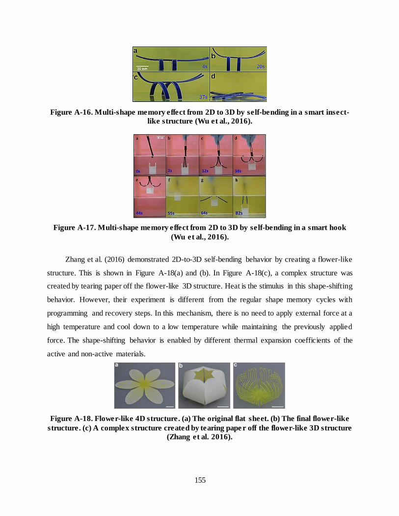
155

Figure A-16. Multi-shape memory effect from 2D to 3D by self-bending in a smart insect-

like structure (Wu et al., 2016).

Figure A-17. Multi-shape memory effect from 2D to 3D by self-bending in a smart hook

(Wu et al., 2016).

Zhang et al. (2016) demonstrated 2D-to-3D self-bending behavior by creating a flower-like

structure. This is shown in Figure A-18(a) and (b). In Figure A-18(c), a complex structure was

created by tearing paper off the flower-like 3D structure. Heat is the stimulus in this shape-shifting

behavior. However, their experiment is different from the regular shape memory cycles with

programming and recovery steps. In this mechanism, there is no need to apply external force at a

high temperature and cool down to a low temperature while maintaining the previously applied

force. The shape-shifting behavior is enabled by different thermal expansion coefficients of the

active and non-active materials.

Figure A-18. Flower-like 4D structure. (a) The original flat sheet. (b) The final flower-like

structure. (c) A complex structure created by tearing pape r off the flower-like 3D structure

(Zhang et al. 2016).

156

In another experiment performed by Zhang et al. (2016), a 3D periodic structure was

achieved from a 2D sheet consisting of four periodic cells in a square arrangement. Each cell

included one central region and four rectangular neighbors, as shown in Figure A-19. The

mechanism of this shape-shifting behavior is similar to that exhibited in the previous experiment.

Figure A-19. A 3D periodic structure created from a 2D sheet by self-bending (Zhang et al.,

2016).

Jamal et al. (2013) illustrated a shape alteration for tissue engineering purposes in which a

2D bio-origami planar pattern changed to a 3D pattern based on the self-bending operation (Figure

A-20). This shape-shifting is enabled by the different swelling ratios of hydrogels and passive

materials under water.

Figure A-20. A bio-origami 2D pattern transforms into a 3D pattern by self-bending: (a)

Schematic illustration of the self-bending of PEG bilayer. (b) A fluorescent micrograph of a

self-bended bilayer (Jamal et al., 2013).

Villar et al. (2013) illustrated 2D-to-3D self-bending behavior in which a flower-shaped

network of droplets transforms into a hollow sphere. This is shown in Figure A-21. This shape-

shifting is enabled by the osmolarity gradient of the droplets described earlier.

157

Figure A-21. (a) The experiment related to 2D-to-3D self-bending in which a flower-shaped

network transforms into a hollow sphere. Scale bar, 200 µm (b) Simulation of (a) (Villar et

al., 2013).


As shown in Figure A-22, Tibbits (2014) printed a 2D flat plane that could be folded into a

closed-surface cube, which presented 2D-to-3D shape-shifting behavior based on self-folding.

This shape-shifting behavior is enabled by a stress mismatch between passive and active materials

due to their different swelling behaviors under water.

Figure A-22. An illustration of 2D to 3D shape-shifting by self-folding to make a cube

(Tibbits, 2014).

The same shape-shifting behavior from a 2D pattern to 3D cube based on self-folding was

also illustrated by Naficy et al. (2017), where both water and heat were required as stimulus. They

printed bilayer hinges made of active and non-active gels. The active layer is a temperature-

sensitive hydrogel. In a dry condition at room temperature, the cube is flat. When submerged in

water at room temperature, the active hydrogel swells and the flat structure is folded. However, if

the temperature of the water is increased above the lower critical solution temperature (LCST) of

158

the active hydrogel, the folded structure unfolds. This occurs because the active hydrogel collapses

above its LCST (which is mainly due to the breaking of the hydrogen bondings).

As shown in Figure A-23, a truncated octahedron was created by Tibbits et al. (2014) and

shows 2D to 3D shape-shifting behavior based on self-folding mechanism. This shape-shifting is

enabled by the stress mismatch between passive and active materials due to their different swelling

ratios.

Figure A-23. 2D-to-3D self-folding to make a truncated octahedron (Tibbits et al., 2014).

Ge et al. (2013) showed self-folding transformations from 2D flat sheets to 3D shapes,

examples of which included an active origami box, pyramid, and airplanes (Figure A-24). These

shape-shifting behaviors are triggered by heat in the usual shape memory cycles with the regular

programming and recovery steps.

Figure A-24. An illustration of a 2D-to-3D alteration in which some origami shapes, such as

an origami box, pyramid, and airplane can be generated by self-folding (Ge et al., 2014).

159

Mao et al. (2015) demonstrated a sequence of self-folding operations for transforming a 2D

strip into 3D shape, as shown in Figure A-25. This shape-shifting behavior is also triggered by

heat in the regular shape memory cycles with programming and recovery steps.

Figure A-25. Sequential self-folding from 2D to 3D (Mao et al., 2015).

• 2D-to-3D Twisting:

Zhang et al. (2016) illustrated helical structures with different spiral degree patterns by

twisting a 2D sheet and converting it to 3D shapes, as shown in Error! Reference source not f

ound.. This shape-shifting behavior has a similar mechanism to that shown in Figure A-18 and

Figure A-19. In addition, Zhang et al. (2018) printed the fibers with certain angles to induce

twisting, and by adjusting the print angles of active fibers, the final twist angle would be changed.

Figure A-26. Helical structures with different degrees of spiral by 2D-to-3D twisting

(Zhang et al., 2016).

• 2D-to-3D Surface Curling:

Tibbits et al. (2014) fabricated a surface grid structure with alternating upper and lower

segments of expandable materials, which could yield a mathematical sinusoidal surface under

water (Figure A-27). This was a demonstration of 2D to 3D shape-shifting behavior with a surface

curling feature. This shape-shifting behavior is enabled by a stress mismatch between passive and

active materials from their different swelling properties under water.

160

Figure A-27. 2D-to-3D sinusoidal shape-shifting by surface curling (Tibbits et al., 2014).

To further illustrate surface curling behavior, hair-like structures were generated from

vertical linear strips by Tibbits et al. (2014) (Figure A-28). The mechanism is the same as above.

Figure A-28. An illustration of 2D-to-3D hair-like shape-shifting by surface curling (Tibbits

et al., 2014).

Raviv et al. (2014) illustrated 2D-to-3D surface curling behavior with various configurations

(Figure A-29). The mechanism is the same as that described above.

Figure A-29. 2D-to-3D surface curling (Raviv et al., 2014).

161

Ge et al. (2013) demonstrated 2D-to-3D shape-shifting behavior in which a flat sheet was

transformed into a complex and non-uniform curvature shape as a sculpture (Figure A-30). This

shape-shifting behavior is triggered by heat in the usual shape memory cycles.

Figure A-30. An illustration of 2D-to-3D alteration in which a complex, non-uniform

curvature sculpture is achieved: (a) Schematic of the flat laminate. (b) The final desired

shape after the thermo-mechanical experiment (Ge et al., 2013).

• 2D-to-3D surface topographical change:

In one experiment from Tibbits et al. (2014), mountain and valley features could be

generated from concentric circles in the presence of an appropriate stimulus (Figure A-31). This

is an illustration of 2D-to-3D change in surface topography. This shape-shifting behavior is

enabled by a stress mismatch between passive and active materials from their different underwater

swelling properties.

Figure A-31. An illustration of 2D-to-3D surface topographical changes where mountains

and valleys are created on a flat surface (Tibbits et al., 2014).

Tibbits et al. (2014) showed another 2D-to-3D surface topographical change in Figure A-32.

In this test, three shapes evolved as a function of time (zero minutes, thirty minutes, and twenty-

four hours in contact with stimulus). These sinusoidal topographies are generated based on the

162

different swelling ratios between the active and passive materials. The concentrations of these

materials vary from the center to the perimeter of the disc.

Figure A-32. 2D-to-3D shape-shifting with surface topography (Tibbits et al., 2014).

• 2D-to-3D Bending and Twisting:

Gladman et al. (2016) demonstrated a combination of 2D-to-3D bending and twisting

behavior with complex flower morphologies. This is produced by the biomimetic 4D printing

process shown in Figure A-33. This shape-shifting behavior is caused by the differences in the

swelling ratios of active and passive materials under water.

Figure A-33. 2D-to-3D shape-shifting by the combination of bending and twisting with

complex flower morphologies (Gladman et al., 2016).

163

Ge et al. (2013) also demonstrated 2D-to-3D bending, twisting, and a combination of the

two, as shown in Figure A-34. This shape-shifting behavior is triggered by heat in the usual shape

memory cycles with the well-known programming and recovery steps.

Figure A-34. Various 2D-to-3D shape-shifting behaviors (Ge et al., 2013).


Kokkinis et al. (2015) showed 3D-to-3D self-bending in a bio-printed structure, as illustrated

in Figure A-35. This shape-shifting behavior is triggered by the dissolution of an appropriate

material into a suitable solvent, which will be further described in the section discussing shape-

shifting mechanisms and stimuli.

Figure A-35. An illustration of 3D-to-3D self-bending in a bio-printed structure (Kokkinis

et al., 2015).

Mutlu et al. (2015) demonstrated the 3D-to-3D self-bending shape-shifting behavior in a

prosthetic finger made from thermoplastic elastomer (TPE), as shown in Figure A-36.

164

Figure A-36. 3D to 3D self-bending in a prosthetic finger (Mutlu et al., 2015).

• 3D-to-3D Linear Deformation

Bakarich et al. (2015) demonstrated 3D-to-3D linear expansion and contraction behavior

(Figure A-37). This shape-shifting behavior is enabled by linear free swelling or shrinkage of a

thermo-responsive hydrogel in the cold or hot water.

Figure A-37. 3D-to-3D shape-shifting by expansion and contraction (Bakarich et al., 2015).

• 3D-to-3D Non-Linear Deformation:

Kuksenok et al. (2016) illustrated the concepts of global and local shrinkage and bending for

3D to 3D shape-shifting behavior. Two stimuli are needed for the global and local shape-shifting

deformation (Figure A-38). The left side of Figure A-38 shows 3D-to-3D bending, while the right

side indicates 3D-to-3D nonlinear shrinkage. The mechanism of this behavior will be described in

further detail in the section discussing shape-shifting mechanisms and stimuli.

Figure A-38. Illustration of global and local shrinkage and bending for 3D-to-3D

alterations by using two different stimuli (Kuksenok et al., 2016).

A.1.6 Discussions

165

In many applications, a 4D printing process can be used to avoid directly printing a

complicated 3D shape. Instead, a lower-dimension shape can be printed first and then the other

dimension(s) can be enabled in the target location with the required performance. Printing a lower-

dimensional object is relatively easy, fast, and has lower manufacturing costs. Furthermore, the

storage and transportation of lower-dimension objects are more convenient. In the study of 2D-to-

3D shape-shifting behavior from Liu et al. (2016), the addition of the third dimension could add

desired value or functions to the 2D substrates, which could be printed with various ordinary

techniques such as inkjet, photolithography, and roll-to-roll printing.

Even though many shape-shifting types and dimensions have been demonstrated in the

literature, hybrid shape-shifting behavior is largely unexplored. Future studies can focus on serial

and parallel combinations of different shape-shifting types and dimensions. For example, a

complex 3D structure can be generated by a designed series of bending and twisting from a 2D

substrate. In some conditions, due to space restrictions, twisting shape-shifting is not directly

accessible until the 2D pattern is first bent into a certain angle. Accordingly, self-bending can be

designed as the first step of the shape-shifting sequence, which allows the structure to access the

target location and then perform the desired twisting.

Sequential shape-shifting behavior can provide more complex actuations. However, all of

the existing sequential shape-shifting studies are limited to folding deformation, whether it is

fabricated from a 4D printing process (Mao et al., 2015; Lee et al., 2015; Baker et al., 2016) or

other manufacturing processes (Laflin et al., 2012; Stoychev et al., 2013; Felton et al., 2013).

Therefore, other sequential shape-shifting types and their combinations can be studied in future

research in this area.

A.2 Applications

The droplets network illustrated by Villar et al. (2013) can be used as tissue engineering

substrates or as support for the functionality of failing tissues (Figure 1-19).

Kokkinis et al. (2015) created smart key–lock connectors (Figure A-39) based on the

experiments shown in Figure A-35. The walls are flat before swelling. After swelling, convex and

concave deformations occur in the wall, which leads to a reduction in the internal size of the cuboid

and finally the interlocking can be achieved. The key-lock connector can be used as a physical

connection between biological parts in the body, such as tendons and muscle. In addition, it can

166

be used as the selective pick-and-place system in soft robots. Soft robotics is one main area, where

4D printing can provide benefits (Wallin et al., 2018).

Figure A-39. Smart key–lock connectors that can be employed for various purposes

(Kokkinis et al., 2015).

Bakarich et al. (2015) fabricated a skeletal muscle-like reversible actuator with high response

speed based on the principle in Figure A-37. They incorporated it into a smart valve (Figure A-40)

and controlled the water flow by self-opening of the valve in cold water and self-closing in hot

water. This work shows one example of 4D printed soft mechanical actuators (Loh, 2016).

Figure A-40. (a) Computer-aided design of the smart valve, (b) Printing of the valve, (c) 4D

printed valve in cold water, and (d) hot water (Bakarich et al., 2015).

Using a different stimulus, Nadgorny et al. (2016) printed a pH-responsive hydrogel valve

that demonstrated dynamic and reversible swelling and shrinkage behavior that could regulate the

167

flow rate under various pH levels (Figure A-41). Additionally, this structure could serve as a useful

platform for pH-responsive membranes (Orlov et al., 2007) and photonic gels (Kang et al., 2007).

Figure A-41. pH-responsive flow regulating smart valve (Nadgorny et al., 2016).

Adaptive metamaterials with tunable bandgaps enabled by 4D printing were reported by

Zhang et al. (2016) (Figure A-42) and later by Bodaghi et al. (2016) (Figure A-43). In both studies,

the lattice structure could be reconfigured in a reversible manner, where heat was the external

stimulus. The fabricated metamaterial shown in Figure A-43 could be applied as planar self-

expanding/shrinking actuators (Bodaghi et al., 2016). The lattice structure demonstrated by Zhang

et al. (2016) (Figure A-42) worked under the unconstrained-thermo-mechanics interaction

mechanism, while the one reported by Bodaghi et al. (2016) (Figure A-43) worked under the

constrained-thermo-mechanics interaction mechanism.

The mechanical properties of metamaterials depend on their geometrical architectures

instead of their chemical compositions (Bodaghi et al., 2016). The adaptive metamaterials with

tunable band gaps are useful for controlling the elastic waves (Zhang et al., 2016). Adaptive

metamaterials can adjust their stiffness based on changes in geometry while keeping their mass

constant. Therefore, they can be used as a switch between two different dynamic states (Bodaghi

et al., 2016).

Figure A-42. Thermo-responsive adaptive metamaterials with tunable bandgaps (Zhang et

al., 2016).

168

Figure A-43. Thermo-responsive adaptive metamaterials with tunable structures (Bodaghi

et al., 2016).

Jiang and Wang (2016) fabricated and analyzed elastomer metamaterials (Figure A-44) that

could be used as reversible shape-shifting connectors. The shape-shifting action is enabled by

external mechanical loadings. These materials can be applied through the 4D printing process to

bridge components for flexible twisting or bending (Jiang & Wang, 2016).

Figure A-44. Elastomer metamaterials (Jiang & Wang, 2016).

Kuksenok et al. (2016) (Figure A-38) developed a 4D-printed structure that could mimic the

contraction of an accordion. They also developed a structure to mimic the lateral movement of a

caterpillar. Their experiments were suitable to manufacture smart components for new adaptive

devices, such as soft robots (Mao et al., 2016).

An active origami box, pyramid, and airplanes illustrated by Ge et al. (2014) show that the

4D printing process is capable of developing smart origami. Origami has attracted a significant

amount of interest lately in an effort to solve engineering issues related to the packing of large

169

structures into small volumes, for the sake of storage and transportation (Ge et al. 2014). In this

regard, Kowk et al. (2015) performed the design optimization of origami for freeform surfaces in

4D printing. In addition, Jamal et al. (2013) (Figure A-20) proposed and fabricated self-bending,

bio-origami structures that could be used in the field of tissue engineering to analyze the behavior

of cells and self-bending vascularized tissue structures. In addition, their findings can be applied

to the field of microfluidic networks (Jamal et al., 2013).

The regeneration of Crambin protein structures through self-folding of a 1D strand in water

was demonstrated by Tibbits et al. (2014) to serve as a potential solution for biomedical problems.

A linear stretching joint, ring stretching joint, and folding joint had been demonstrated by Raviv

et al. (2014). These joints could be used in other structures in practice. The development of a fully

compliant prosthetic finger was another application that was demonstrated by Mutlu et al. (2015)

(Figure A-36).

Wu et al. (2016) showed several smart structures including a smart hook, smart trestle, and

a smart insect-like structure so that after the thermomechanical cycle, the structure could undergo

shape-shifting between a planar shape and the desired hook, trestle, and insect-like shapes.

A 4D-printed, thermo-responsive, SMP-based, cardiovascular stent was fabricated by Ge et

al. (2016) (Figure A-45). Stents are important devices to expand the human vessels and has been

the focus of many studies from different perspectives (Anand et al., 2009; Yakacki et al., 2007;

Yakacki et al., 2008). Traditional fabrication methods are difficult and time-consuming in

providing complex geometries with high resolutions required by stents (Yakacki et al., 2007;

Srivastava et al., 2010). Based on a high resolution PμSL additive manufacturing system, Ge et al.

(2016) could manufacture the high-resolution stents with various diameters, heights, number of

joints, ligament diameters, and inter-ligament angles. Similarly, a 4D-printed thermo-responsive

stent (Figure A-46) was demonstrated by Bodaghi et al. (2016), in which the stent diameter could

be changed reversibly while the height was kept constant. Both stents (Figure A-45 and Figure

A-46) worked under the constrained-thermo-mechanics interaction mechanism. Wei et al. (2016)

incorporated Fe3O4 in a thermo-responsive PLA-based ink and 4D printed a smart stent which

could be guided magnetically and actuated remotely.

170

Figure A-45. A 4D-printed, thermo-responsive stent which is able to reversibly change its

diameter and height (Ge et al., 2016).

Figure A-46. A 4D-printed, thermo-responsive stent which is able to reversibly change its

diameter (Bodaghi et al., 2016).

Zarek et al. (2016) 4D printed a thermo-responsive tracheal stent (Figure A-47), which

solved two issues related with the current tracheal stents. First, it fits the arcade pattern and

cartilaginous rings better and provides a stable state, which prevents migrations. Second, the

shrunk form during insertion prevents the injurious insertion. After being inserted into the body,

the tracheal stent can expand to the permanent shape with a local increment in temperature (Zarek

et al., 2016).

171

Figure A-47. 4D printed thermo-responsive tracheal stent (Zarek et al., 2016).

Ge et al. (2016) developed a SMP-based thermo-responsive multimaterial gripper, as shown

in Figure A-48, which can be applied in drug delivery systems (DDS) (Malachowski et al., 2014).

Figure A-48. 4D-printed shape memory gripper that can reversibly grab and release the

objects by heat (Ge et al., 2016).

Self-adaptive and multi-functional textiles are some of the potential applications that can be

improved by 4D printing (Truby & Lewis, 2016). Self-adaptive smart textile structure can be

adapted to a new size without tensile loading, in contrast to the textiles made of elastic fibers

(Figure A-49) (Hu et al., 2012). Multi-functional smart textiles are capable of managing the

moisture or temperature of the body, monitoring wounds, providing skin care, protecting against

harsh climates, or adaptively changing color of a dress (Hu et al., 2012).

172

Figure A-49. Adaptability of textiles made of SMP vs. the textiles made of elastic fibers (Hu

et al., 2012).

4D bio-printing (An et al., 2015; Gao et al., 2016) of stem cells directly into scaffolds is a

significant advancement toward the creation of organs and tissues. The stimulation of stem cell

differentiation can provide shape-shifting behavior in a 4D printed scaffold (Irvine & Venkatraman,

2016; Miao et al., 2016; Wei et al., 2016). Laser-based cell printing (Koch et al., 2016) can pave

the way for 4D bio-printing of cells.

Recently, a 4D nano-printing process was demonstrated by Carbonell and Braunschweig

(2016). The bottom-up 4D nano-printing process is expected to be an effective alternative to the

conventional top-down techniques used for fabricating electronics, bioarrays, and functional

substrates. Future developments in this area depend on further developments in surface chemistry

and instrumentation (Carbonell & Braunschweig, 2016).

The additive construction of buildings can make a significant contribution to the construction

industry (Labonnote et al., 2016). One of the primary technologies in this field is contour crafting

(CC) (Khoshnevis, 2004). As Khoshnevis mentioned, the purpose of CC is the automated

construction of one house or a colony of houses in a single run using layered manufacturing

techniques (Figure A-50). CC is one of the few feasible methods for construction on planets in

outer space, such as Mars (Khoshnevis, 2004). On the other hand, 4D printing can fabricate smart

elements as building blocks that can be self-assembled after printing. Therefore, as Labonnote et

173

al. (2016) indicated, 4D printing and contour crafting can effectively complement each other to

pave the way for the human colonization on Mars. One of the main challenges in 4D printed

structures is that after a certain number of shape-shifting cycles, the 4D printed structure cannot

effectively recover its original shape and degrades (Raviv et al., 2014). In addition to the

degradation modeling and lifespan monitoring of 4D printed structures (Momeni et al., 2016),

future studies should focus on the improvement of their lifespan.

Figure A-50. Automated construction of a building in a single run using contour crafting

technology (Khoshnevis, 2004).

In summary, 4D printing process applications are summarized in Figure A-51, along with

the associated literature.

174

Figure A-51. Applications of the 4D printing process.

4D printing applications

Demonstrated applications Potential applications


• Bodaghi et al. (2016)

• Jiang and Wang (2016)

Adaptive meta-

materials

Artificial Crambin

protein structure Tibbits et al. (2014)

Construction on Mars along

with Contour Crafting Labonnote et al. (2016)

4D nanoprinting Carbonell and

Braunschweig (2016)Smart valve to control

the hot and cold flow Bakarich et al. (2015)

Smart valve to control

the acidic or basic flow Nadgorny et al. (2016)

Drug delivery systems Ge et al. (2016)

Smart textiles Truby and Lewis (2016)

Laser-based cell printing Koch et al. (2016)

Origami structures Ge et al. (2014)

Bio-origami Jamal et al. (2013)

Stent • Ge et al. (2016); Bodaghi et al. (2016)

• Zarek et al. (2016); Wei et al. (2016)

Adaptive pipes Campbell et al. (2014)

Self-healing hydrogels Taylor et al. (2016)

Self-assembly at large scales

and in the harsh environmentTibbits et al. (2014)

Soft robots • Kuksenok et al. (2016)


Smart gripper Ge et al. (2016)

Smart key–lock connectors Kokkinis et al. (2015)

Adaptive joints Raviv et al. (2014)

Adaptive Scaffolds• Miao et al. (2016)

• Wei et al. (2016)

Tissue engineering

• Villar et al. (2013)

• Khademhosseini & Langer (2016)

• Jung et al. (2016)

Error-correct and self-

repairing structuresTibbits (2014)

175

BIBLIOGRAPHY

Ali, I. M. S., O’Donovan, T. S., Reddy, K. S., & Mallick, T. K. (2013). An optical analysis of a

static 3-D solar concentrator. Solar Energy, 88, 57-70.

Alipour, N., Andersson, R. L., Olsson, R. T., Gedde, U. W., & Hedenqvist, M. S. (2016). VOC-Induced Flexing of Single and Multilayer Polyethylene Films As Gas Sensors. ACS applied materials & interfaces, 8(15), 9946-9953.

Al-Shohani, W. A., Al-Dadah, R., Mahmoud, S., & Algareu, A. (2016). Optimum design of V-trough concentrator for photovoltaic applications. Solar Energy, 140, 241-254.

Amanlou, Y., Hashjin, T. T., Ghobadian, B., Najafi, G., & Mamat, R. (2016). A comprehensive review of uniform solar illumination at low concentration photovoltaic (lcpv)

systems. Renewable and Sustainable Energy Reviews, 60, 1430-1441.

Amano, R. S., & Sundén, B. (Eds.). (2014). Aerodynamics of wind turbines: emerging topics. WIT Press.

An, J., Teoh, J. E. M., Suntornnond, R., & Chua, C. K. (2015). Design and 3D printing of

scaffolds and tissues. Engineering, 1(2), 261-268.

Anand, L., Ames, N. M., Srivastava, V., & Chester, S. A. (2009). A thermo-mechanically coupled theory for large deformations of amorphous polymers. Part I: Formulation. International Journal of Plasticity, 25(8), 1474-1494.

Apostoleris, H., Stefancich, M., & Chiesa, M. (2016). Tracking-integrated systems for concentrating photovoltaics. Nature Energy, 1, 16018.

Ashwill, T. D. (2010). Sweep-twist adaptive rotor blade: final project report (No. SAND2009-8037). Sandia National Laboratories.

Ashwill, T., Kanaby, G., Jackson, K., & Zuteck, M. (2010). Development of the sweep-twist adaptive rotor (STAR) blade. In 48th AIAA Aerospace Sciences Meeting Including the New Horizons Forum and Aerospace Exposition (p. 1582).

Athanasopoulos, N., & Siakavellas, N. (2018, July). Variable emissivity through multilayer

patterned surfaces for passive thermal control: preliminary thermal design of a nano-

176

satellite. 48th International Conference on Environmental Systems. Albuquerque, New Mexico

Athanasopoulos, N., & Siakavellas, N. J. (2017). Smart patterned surfaces with programmable

thermal emissivity and their design through combinatorial strategies. Scientific reports, 7(1), 12908.

Avella, M., Buzarovska, A., Errico, M. E., Gentile, G., & Grozdanov, A. (2009). Eco-challenges of bio-based polymer composites. Materials, 2(3), 911-925.

Avid, A. Types of Flowers That Close at Night. Available at: http://homeguides.sfgate.com/types-flowers-close-night-56308.html (accessed July 2017).

Bakarich, S. E., Gorkin, R., & Spinks, G. M. (2015). 4D printing with mechanically robust,

thermally actuating hydrogels. Macromolecular rapid communications, 36(12), 1211-1217.

Baker, A. B., Wass, D. F., & Trask, R. S. (2016). 4D sequential actuation: combining ionoprinting and redox chemistry in hydrogels. Smart Materials and Structures, 25(10),

10LT02.

Bandyopadhyay, A., & Heer, B. (2018). Additive manufacturing of multi-material structures. Materials Science and Engineering: R: Reports, 129, 1-16.

Barthlott, W., Mail, M., Bhushan, B., & Koch, K. (2017). Plant surfaces: structures and functions

for biomimetic innovations. Nano-Micro Letters, 9(2), 23.

Bazilevs, Y., Hsu, M. C., Kiendl, J., & Benson, D. J. (2012). A computational procedure for prebending of wind turbine blades. International Journal for Numerical Methods in Engineering, 89(3), 323-336.

Behl, M., & Lendlein, A. (2007). Shape-memory polymers. Materials today, 10(4), 20-28.

Bejan, A. (2016). Advanced engineering thermodynamics. John Wiley & Sons.

Bellos, E., & Tzivanidis, C. (2017). Parametric analysis and optimization of an Organic Rankine Cycle with nanofluid based solar parabolic trough collectors. Renewable Energy, 114,

1376-1393.

Bensaude-Vincent, B. Self-Assembly, Self-Organization: A Philosophical Perspective on Converging Technologies Paper prepared for France/Stanford Meeting Avignon, December 2006.

Berens, A. R., & Hopfenberg, H. B. (1978). Diffusion and relaxation in glassy polymer powders: 2. Separation of diffusion and relaxation parameters. Polymer, 19(5), 489-496.

http://homeguides.sfgate.com/types-flowers-close-night-56308.html

177

Bergström, L. M. (2011). Thermodynamics of self-assembly. In Application of Thermodynamics to Biological and Materials Science. InTech.

Best, J. P., Neubauer, M. P., Javed, S., Dam, H. H., Fery, A., & Caruso, F. (2013). Mechanics of

pH-responsive hydrogel capsules. Langmuir, 29(31), 9814-9823.

Bir, G., & Jonkman, J. (2007). Aeroelastic instabilities of large offshore and onshore wind turbines. In Journal of Physics: Conference Series (Vol. 75, No. 1, p. 012069). IOP Publishing.

Blees, M. K., Barnard, A. W., Rose, P. A., Roberts, S. P., McGill, K. L., Huang, P. Y., ... & McEuen, P. L. (2015). Graphene kirigami. Nature, 524(7564), 204.

Bodaghi, M., Damanpack, A. R., & Liao, W. H. (2016). Self-expanding/shrinking structures by 4D printing. Smart Materials and Structures, 25(10), 105034.

Bongers, P. M., & van Baars, G. E. (1991, December). Experimental validation of a flexible wind turbine model. In Decision and Control, 1991., Proceedings of the 30th IEEE Conference on (pp. 1660-1661). IEEE.

Bonner, M., de Oca, H. M., Brown, M., & Ward, I. M. (2010). A novel approach to predict the

recovery time of shape memory polymers. Polymer, 51(6), 1432-1436.

Bottasso, C. L., Campagnolo, F., Croce, A., & Tibaldi, C. (2013). Optimization‐based study of bend–twist coupled rotor blades for passive and integrated passive/active load alleviation. Wind Energy, 16(8), 1149-1166.

Branham, M., Gutowski, T. G., Jones, A., & Sekulic, D. P. (2008, May). A thermodynamic framework for analyzing and improving manufacturing processes. In Electronics and the Environment, 2008. ISEE 2008. IEEE International Symposium on (pp. 1-6). IEEE.

Brøndsted, P., Lilholt, H., & Lystrup, A. (2005). Composite materials for wind power turbine

blades. Annu. Rev. Mater. Res., 35, 505-538.

Bunse, K., Vodicka, M., Schönsleben, P., Brülhart, M., & Ernst, F. O. (2011). Integrating energy efficiency performance in production management–gap analysis between industrial needs and scientific literature. Journal of Cleaner Production, 19(6-7), 667-679.

Campbell, T. A., Tibbits, S., & Garrett, B. (2014). The programmable world. Scientific American, 311(5), 60-65.

Carbonell, C., & Braunschweig, A. B. (2016). Toward 4D nanoprinting with tip-induced organic surface reactions. Accounts of chemical research, 50(2), 190-198.

Carter, K. Plants That Open in Sunlight & Close in Dark. Available at: http://homeguides.sfgate.com/plants-open-sunlight-close-dark-28050.html (accessed July 2017).

http://homeguides.sfgate.com/plants-open-sunlight-close-dark-28050.html

178

Cengel, Y. A., & Boles, M. A. (2015). Thermodynamics: An engineering approach . New York: McGraw-Hill Education.

Chaves, J. (2015). Introduction to nonimaging optics. CRC press.

Chehouri, A., Younes, R., Ilinca, A., & Perron, J. (2015). Review of performance optimization techniques applied to wind turbines. Applied Energy, 142, 361-388.

Chen, L., Harding, C., Sharma, A., & MacDonald, E. (2016). Modeling noise and lease soft costs improves wind farm design and cost-of-energy predictions. Renewable Energy, 97, 849-

859.

Choi, J., Kwon, O. C., Jo, W., Lee, H. J., & Moon, M. W. (2015). 4D printing technology: A review. 3D Printing and Additive Manufacturing, 2(4), 159-167.

Choong, Y. Y. C., Maleksaeedi, S., Eng, H., Wei, J., & Su, P. C. (2017). 4D printing of high

performance shape memory polymer using stereolithography. Materials & Design, 126, 219-225.

Cock, F., Cuadri, A. A., García-Morales, M., & Partal, P. (2013). Thermal, rheological and microstructural characterisation of commercial biodegradable polyesters. Polymer

Testing, 32(4), 716-723.

Cock, F., Cuadri, A. A., García-Morales, M., & Partal, P. (2013). Thermal, rheological and microstructural characterisation of commercial biodegradable polyesters. Polymer Testing, 32(4), 716-723.

Cognet, V., du Pont, S. C., Dobrev, I., Massouh, F., & Thiria, B. (2017, February). Bioinspired turbine blades offer new perspectives for wind energy. In Proc. R. Soc. A (Vol. 473, No. 2198, p. 20160726). The Royal Society.

Čolić-Damjanovic, V. M., & Gadjanski, I. (2016, September). Potentials of fablabs for

biomimetic architectural research. In Multidisciplinary Engineering Design Optimization (MEDO), International Conference (pp. 1-6). IEEE.

Corten, G. P., & Veldkamp, H. F. (2001). Aerodynamics: Insects can halve wind-turbine power. Nature, 412(6842), 41-42.

Costabile, G., Fera, M., Fruggiero, F., Lambiase, A., & Pham, D. (2017). Cost models of additive manufacturing: A literature review. International Journal of Industrial Engineering Computations, 8(2), 263-283.

Costello, H. (2018). 3D and 4D Printing Market: Latest Technology, Industry Demand, Future

Growth Opportunities till 2022 by Key Players and Regional Analysis. Orbis Research. Available at: https://www.reuters.com/brandfeatures/venture-capital/article?id=29519.

https://www.reuters.com/brandfeatures/venture-capital/article?id=29519

179

Czugala, M., O’Connell, C., Blin, C., Fischer, P., Fraser, K. J., Benito-Lopez, F., & Diamond, D. (2014). Swelling and shrinking behaviour of photoresponsive phosphonium-based ionogel microstructures. Sensors and Actuators B: Chemical, 194, 105-113.

Dai, G., & Mishnaevsky, L. (2014). Fatigue of hybrid glass/carbon composites: 3D computational studies. Composites Science and Technology, 94, 71-79.

Daneshazarian, R., Cuce, E., Cuce, P. M., & Sher, F. (2018). Concentrating photovoltaic thermal (CPVT) collectors and systems: Theory, performance assessment and

applications. Renewable and Sustainable Energy Reviews, 81, 473-492.

De Goeij, W. C., Van Tooren, M. J. L., & Beukers, A. (1999). Implementation of bending-torsion coupling in the design of a wind-turbine rotor-blade. Applied Energy, 63(3), 191-207.

De Volder, M. F., Tawfi ck, S. H., Baughman, R. H., & Hart, A. J. (2013). Carbon nanotubes: present and future commercial applications. science, 339(6119), 535-539.

Dekker, H. Saxifraga. Available at: http://www.freenatureimages.eu/plants/Flora%20O-R/Ranunculus%20auricomus,%20Goldilocks%20Buttercup/index.html (accessed

December 2017).

Demir, A. G., & Previtali, B. (2017). Multi-material selective laser melting of Fe/Al-12Si components. Manufacturing letters, 11, 8-11.

Dicker, M. P., Duckworth, P. F., Baker, A. B., Francois, G., Hazzard, M. K., & Weaver, P. M.

(2014). Green composites: A review of material attributes and complementary applications. Composites part A: applied science and manufacturing, 56, 280-289.

Ding, Z., Yuan, C., Peng, X., Wang, T., Qi, H. J., & Dunn, M. L. (2017). Direct 4D printing via active composite materials. Science advances, 3(4), e1602890.

Dodge, DM. (2006). The illustrated history of wind power development. Littleton, Colorado: U.S. Federal Wind Energy Program. Available at: http://www.telosnet.com/wind/early.html (accessed July 2017).

Dong, Y., Ghataura, A., Takagi, H., Haroosh, H. J., Nakagaito, A. N., & Lau, K. T. (2014).

Polylactic acid (PLA) biocomposites reinforced with coir fibres: Evaluation of mechanical performance and multifunctional properties. Composites Part A: Applied Science and Manufacturing, 63, 76-84.

Drumheller, D. P., D’Antonio, G. C., Chapman, B. A., Allison, C. P., & Pierrakos, O. (2015,

April). Design of a micro-wind turbine for implementation in low wind speed environments. In Systems and Information Engineering Design Symposium (SIEDS), 2015 (pp. 125-130). IEEE.

Drumright, R. E., Gruber, P. R., & Henton, D. E. (2000). Polylactic acid technology. Advanced

materials, 12(23), 1841-1846.

http://www.freenatureimages.eu/plants/Flora%20O-R/Ranunculus%20auricomus,%20Goldilocks%20Buttercup/index.html

http://www.freenatureimages.eu/plants/Flora%20O-R/Ranunculus%20auricomus,%20Goldilocks%20Buttercup/index.html

http://www.telosnet.com/wind/early.html

180

Duerr, F., Meuret, Y., & Thienpont, H. (2011). Tracking integration in concentrating photovoltaics using laterally moving optics. Optics express, 19(103), A207-A218.

Duffy, S. (2010). Linear Viscoelasticity: Mechanical (rheological) models. Lecture notes,

Cleveland State University. Available at: http://academic.csuohio.edu/duffy_s/Linear_Visco.pdf (accessed December 2017).

Dwyer Instruments Inc. (2010). Product Categories. Retrieved May 29, 2017. Available at: https://www.dwyer-inst.com/PDF_files/400_IOM.pdf (accessed July 2017).

El Alaoui, R., Mounir, H., Boudi, E. M., El Marjani, A., Echab, H., & Mohsine, A. (2016, November). Performances comparison of wind turbine blades materials. In Renewable and Sustainable Energy Conference (IRSEC), 2016 International (pp. 375-380). IEEE.

Ellis, A. G., & Johnson, S. D. (2010). Floral mimicry enhances pollen export: the evolution of

pollination by sexual deceit outside of the Orchidaceae. The American Naturalist, 176(5), E143-E151.

ElMaraghy, H. A., Youssef, A. M., Marzouk, A. M., & ElMaraghy, W. H. (2017). Energy use analysis and local benchmarking of manufacturing lines. Journal of Cleaner Production,

163, 36-48.

Eriksson, S., Bernhoff, H., & Leijon, M. (2008). Evaluation of different turbine concepts for wind power. Renewable and Sustainable Energy Reviews, 12(5), 1419-1434.

Esteban, M. D., Diez, J. J., López, J. S., & Negro, V. (2011). Why offshore wind energy?.

Renewable Energy, 36(2), 444-450.

Fedorov, V., & Berggreen, C. (2014). Bend-twist coupling potential of wind turbine blades. In Journal of Physics: Conference Series (Vol. 524, No. 1, p. 012035). IOP Publishing.

Felton, S. M., Tolley, M. T., Shin, B., Onal, C. D., Demaine, E. D., Rus, D., & Wood, R. J.

(2013). Self-folding with shape memory composites. Soft Matter, 9(32), 7688-7694.

Foster, James J., Camilla R. Sharkey, Alicia VA Gaworska, Nicholas W. Roberts, Heather M. Whitney, and Julian C. Partridge. "Bumblebees learn polarization patterns." Current Biology 24, no. 12 (2014): 1415-1420.

Frewer, L. J., Norde, W., Fischer, A., & Kampers, F. (Eds.). (2011). Nanotechnology in the agri-food sector: implications for the future. John Wiley & Sons.

Fritz, B., Hünig, R., Schmager, R., Hetterich, M., Lemmer, U., & Gomard, G. (2017). Assessing the influence of structural disorder on the plant epidermal cells’ optical properties: a

numerical analysis. Bioinspiration & Biomimetics, 12(3), 036011.

Frohm, B., DeNizio, J. E., Lee, D. S. M., Gentile, L., Olsson, U., Malm, J., ... & Linse, S. (2015). A peptide from human semenogelin I self-assembles into a pH-responsive hydrogel. Soft Matter, 11(2), 414-421.

http://academic.csuohio.edu/duffy_s/Linear_Visco.pdf

https://www.dwyer-inst.com/PDF_files/400_IOM.pdf

181

Gao, B., Yang, Q., Zhao, X., Jin, G., Ma, Y., & Xu, F. (2016). 4D bioprinting for biomedical applications. Trends in biotechnology, 34(9), 746-756.

Gardenia. Available at: https://www.gardenia.net/plant/crocus-vernus-flower-record-dutch-

crocus (accessed July 2017).

Garlotta, D. (2001). A literature review of poly (lactic acid). Journal of Polymers and the Environment, 9(2), 63-84.

Ge, Q., Dunn, C. K., Qi, H. J., & Dunn, M. L. (2014). Active origami by 4D printing. Smart

Materials and Structures, 23(9), 094007.

Ge, Q., Qi, H. J., & Dunn, M. L. (2013). Active materials by four-dimension printing. Applied Physics Letters, 103(13), 131901.

Ge, Q., Sakhaei, A. H., Lee, H., Dunn, C. K., Fang, N. X., & Dunn, M. L. (2016). Multimaterial

4D printing with tailorable shape memory polymers. Scientific reports, 6, 31110.

Ghasemi, S. E., & Ranjbar, A. A. (2017). Numerical thermal study on effect of porous rings on performance of solar parabolic trough collector. Applied Thermal Engineering, 118, 807-816.

Girard, R., Laquaine, K., & Kariniotakis, G. (2013). Assessment of wind power predictability as a decision factor in the investment phase of wind farms. Applied Energy, 101, 609-617.

Gladman, A. S., Matsumoto, E. A., Nuzzo, R. G., Mahadevan, L., & Lewis, J. A. (2016). Biomimetic 4D printing. Nature materials, 15(4), 413-418.

Gong, X. L., Xiao, Y. Y., Pan, M., Kang, Y., Li, B. J., & Zhang, S. (2016). pH-and Thermal-Responsive Multishape Memory Hydrogel. ACS applied materials & interfaces, 8(41), 27432-27437.

Gorjian, S., Ghobadian, B., Hashjin, T. T., & Banakar, A. (2014). Experimental performance

evaluation of a stand-alone point-focus parabolic solar still. Desalination, 352, 1-17.

Grant, L. (1987). Diffuse and specular characteristics of leaf reflectance. Remote Sensing of Environment, 22(2), 309-322.

Gratson, G. M., & Lewis, J. A. (2005). Phase behavior and rheological properties of

polyelectrolyte inks for direct-write assembly. Langmuir, 21(1), 457-464.

Griffin, D. A. (2002). Evaluation of design concepts for adaptive wind turbine blades. Sandia National Laboratories, Report No. SAND2002-2424.

Guo, S. Z., Gosselin, F., Guerin, N., Lanouette, A. M., Heuzey, M. C., & Therriault, D. (2013).

Solvent‐Cast Three‐Dimensional Printing of Multifunctional Microsystems. Small, 9(24), 4118-4122.

https://www.gardenia.net/plant/crocus-vernus-flower-record-dutch-crocus

https://www.gardenia.net/plant/crocus-vernus-flower-record-dutch-crocus

182

Gutowski, T. G., Branham, M. S., Dahmus, J. B., Jones, A. J., Thiriez, A., & Sekulic, D. P. (2009). Thermodynamic analysis of resources used in manufacturing processes. Environmental science & technology, 43(5), 1584-1590.

Gutowski, T., Dahmus, J., & Thiriez, A. (2006, May). Electrical energy requirements for manufacturing processes. In 13th CIRP international conference on life cycle engineering (Vol. 31, pp. 623-638). CIRP International Leuven, Belgium.

Gutowski, T., Dahmus, J., Thiriez, A., Branham, M., & Jones, A. (2007, May). A

thermodynamic characterization of manufacturing processes. In Electronics & the Environment, Proceedings of the 2007 IEEE International Symposium on (pp. 137-142). IEEE.

Gyftopoulos, E. P., & Beretta, G. P. (2005). Thermodynamics: foundations and applications.

Courier Corporation.

Hager, M. D., Bode, S., Weber, C., & Schubert, U. S. (2015). Shape memory polymers: past, present and future developments. Progress in Polymer Science, 49, 3-33.

Hansen, M. (2011, January). Aeroelastic properties of backward swept blades. In 49th AIAA

Aerospace Sciences Meeting Including the New Horizons Forum and Aerospace Exposition (p. 260).

Hayat, K., & Ha, S. K. (2015). Load mitigation of wind turbine blade by aeroelastic tailoring via unbalanced laminates composites. Composite Structures, 128, 122-133.

Hayat, K., de Lecea, A. G. M., Moriones, C. D., & Ha, S. K. (2016). Flutter performance of bend–twist coupled large-scale wind turbine blades. Journal of Sound and Vibration, 370, 149-162.

He, S., Chen, P., Sun, X., & Peng, H. (2016). Stimuli-Responsive Materials From Carbon

Nanotubes. Industrial Applications of Carbon Nanotubes, 151.

Heald, M. A. (1992). Uncertainty of the slope for highly correlated data. American Journal of Physics, 60(1), 11-11. of the slope for highly correlated data. American Journal of Physics, 60(1), 11-11.

Hedenstrom, A., & Liechti, F. E. L. I. X. (2001). Field estimates of body drag coefficient on the basis of dives in passerine birds. Journal of Experimental Biology, 204(6), 1167-1175.

Hiller, J., & Lipson, H. (2009). Design and analysis of digital materials for physical 3D voxel printing. Rapid Prototyping Journal, 15(2), 137-149.

Hiller, J., & Lipson, H. (2010). Tunable digital material properties for 3D voxel printers. Rapid Prototyping Journal, 16(4), 241-247.

183

Hirano, A., Hashimoto, T., Kitagawa, D., Kono, K., & Kobatake, S. (2017). Dependence of Photoinduced Bending Behavior of Diarylethene Crystals on Ultraviolet Irradiation Power. Crystal Growth & Design, 17(9), 4819-4825.

Hohmann-Marriott, M. F. (Ed.). (2014). The structural basis of biological energy generation (Vol. 39). Springer Science & Business.

Holmes, J. W., Brøndsted, P., Sørensen, B. F., Jiang, Z., Sun, Z., & Chen, X. (2009). Development of a bamboo-based composite as a sustainable green material for wind

turbine blades. Wind Engineering, 33(2), 197-210.

Hoogedoorn, E., Jacobs, G. B., & Beyene, A. (2010). Aero-elastic behavior of a flexible blade for wind turbine application: A 2D computational study. Energy, 35(2), 778-785.

Howell, R., Qin, N., Edwards, J., & Durrani, N. (2010). Wind tunnel and numerical study of a

small vertical axis wind turbine. Renewable energy, 35(2), 412-422.

Hu, J., Meng, H., Li, G., & Ibekwe, S. I. (2012). A review of stimuli-responsive polymers for smart textile applications. Smart Materials and Structures, 21(5), 053001.

Huang, L., Jiang, R., Wu, J., Song, J., Bai, H., Li, B., ... & Xie, T. (2017). Ultrafast digital

printing toward 4D shape changing materials. Advanced Materials, 29(7).

Ichter, B., Steele, A., Loth, E., Moriarty, P., & Selig, M. (2016). A morphing downwind‐aligned rotor concept based on a 13‐MW wind turbine. Wind Energy, 19(4), 625-637.

IEA, 2007a. Tracking Industrial, Energy Efficiency and CO2 Emissions. Available at:

https://www.iea.org/publications/freepublications/publication/tracking_emissions.pdf (Accessed May 2018).

Irvine, S. A., & Venkatraman, S. S. (2016). Bioprinting and differentiation of stem cells. Molecules, 21(9), 1188.

Jacobsen, M. (2016). Clearing the Way for Pivotal 21st-Century Innovation. In Giftedness and Talent in the 21st Century (pp. 163-179). SensePublishers.

Jacobson, M. Z., & Archer, C. L. (2012). Saturation wind power potential and its implications for wind energy. Proceedings of the National Academy of Sciences, 109(39), 15679-

15684.

Jamal, M., Kadam, S. S., Xiao, R., Jivan, F., Onn, T. M., Fernandes, R., ... & Gracias, D. H. (2013). Bio‐Origami Hydrogel Scaffolds Composed of Photocrosslinked PEG Bilayers. Advanced healthcare materials, 2(8), 1142-1150.

Jespersen, K. M., & Mikkelsen, L. P. (2017). Three dimensional fatigue damage evolution in non-crimp glass fibre fabric based composites used for wind turbine blades. Composites Science and Technology, 153, 261-272.

https://www.iea.org/publications/freepublications/publication/tracking_emissions.pdf

184

Ji, S., & Chen, B. (2016). Carbon footprint accounting of a typical wind farm in China. Applied Energy, 180, 416-423.

Jiang, Y., & Wang, Q. (2016). Highly-stretchable 3D-architected mechanical

metamaterials. Scientific reports, 6, 34147.

Jin, Y., Qin, S. J., & Huang, Q. (2016, August). Prescriptive analytics for understanding of out-of-plane deformation in additive manufacturing. In Automation Science and Engineering (CASE), 2016 IEEE International Conference on(pp. 786-791). IEEE.

Jung, J. P., Bhuiyan, D. B., & Ogle, B. M. (2016). Solid organ fabrication: comparison of decellularization to 3D bioprinting. Biomaterials research, 20(1), 27.

Kaldellis, J. K., & Zafirakis, D. (2011). The wind energy (r) evolution: A short review of a long history. Renewable Energy, 36(7), 1887-1901.

Kang, Y., Walish, J. J., Gorishnyy, T., & Thomas, E. L. (2007). Broad-wavelength-range chemically tunable block-copolymer photonic gels. Nature Materials, 6(12), 957.

Karathanassis, I. K., Papanicolaou, E., Belessiotis, V., & Bergeles, G. C. (2017). Design and experimental evaluation of a parabolic-trough concentrating photovoltaic/thermal

(CPVT) system with high-efficiency cooling. Renewable Energy, 101, 467-483.

Kasaeian, A., Nouri, G., Ranjbaran, P., & Wen, D. (2018). Solar collectors and photovoltaics as combined heat and power systems: A critical review. Energy Conversion and Management, 156, 688-705.

Kaviany, M. (2011). Essentials of heat transfer: principles, materials, and applications . Cambridge University Press.

Khademhosseini, A., & Langer, R. (2016). A decade of progress in tissue engineering. Nature protocols, 11(10), 1775-1781.

Khakrah, H., Shamloo, A., & Hannani, S. K. (2017). Determination of Parabolic Trough Solar Collector Efficiency Using Nanofluid: A Comprehensive Numerical Study. Journal of Solar Energy Engineering, 139(5), 051006.

Khamooshi, M., Salati, H., Egelioglu, F., Hooshyar Faghiri, A., Tarabishi, J., & Babadi, S.

(2014). A review of solar photovoltaic concentrators. International Journal of Photoenergy, 2014, Article 958521.

Khoo, Z. X., Teoh, J. E. M., Liu, Y., Chua, C. K., Yang, S., An, J., ... & Yeong, W. Y. (2015). 3D printing of smart materials: A review on recent progresses in 4D printing. Virtual and

Physical Prototyping, 10(3), 103-122.

Khoshnevis, B. (2004). Automated construction by contour crafting—related robotics and information technologies. Automation in construction, 13(1), 5-19.

185

Kim, B., La Flamme, K., & Peppas, N. A. (2003). Dynamic swelling behavior of pH‐sensitive anionic hydrogels used for protein delivery. Journal of Applied Polymer Science, 89(6), 1606-1613.

Kim, J. M., & Dutta, P. S. (2012). Optical efficiency–concentration ratio trade-off for a flat panel photovoltaic system with diffuser type concentrator. Solar Energy Materials and Solar Cells, 103, 35-40.

Kishore, R. A., Coudron, T., & Priya, S. (2013). Small-scale wind energy portable turbine

(SWEPT). Journal of Wind Engineering and Industrial Aerodynamics, 116, 21-31.

Koch, L., Deiwick, A., & Chichkov, B. (2016). Laser-Based Cell Printing. 3D Printing and Biofabrication, 1-27.

Kokkinis, D., Schaffner, M., & Studart, A. R. (2015). Multimaterial magnetically assisted 3D

printing of composite materials. Nature communications, 6, 8643.

Kooi, C. J., Wilts, B. D., Leertouwer, H. L., Staal, M., Elzenga, J. T. M., & Stavenga, D. G. (2014). Iridescent flowers? Contribution of surface structures to optical signaling. New Phytologist, 203(2), 667-673.

Krawczyk, P., Beyene, A., & MacPhee, D. (2013). Fluid structure interaction of a morphed wind turbine blade. International Journal of Energy Research, 37(14), 1784-1793.

Krogsgaard, M., Behrens, M. A., Pedersen, J. S., & Birkedal, H. (2013). Self-healing mussel-inspired multi-pH-responsive hydrogels. Biomacromolecules, 14(2), 297-301.

Kruth, J. P., Leu, M. C., & Nakagawa, T. (1998). Progress in additive manufacturing and rapid prototyping. CIRP Annals-Manufacturing Technology, 47(2), 525-540.

Kuethe, A. M., & Chow, C. Y. (1976). Fondations of aerodynamics. John Wiley & Sons.

Kuksenok, O., & Balazs, A. C. (2016). Stimuli-responsive behavior of composites integrating

thermo-responsive gels with photo-responsive fibers. Materials Horizons, 3(1), 53-62.

Kwok, T. H., & Chen, Y. (2017). GDFE: Geometry-Driven Finite Element for Four-Dimensional Printing. Journal of Manufacturing Science and Engineering, 139(11), 111006.

Kwok, T. H., Wang, C. C., Deng, D., Zhang, Y., & Chen, Y. (2015). Four-dimensional printing

for freeform surfaces: design optimization of origami and kirigami structures. Journal of Mechanical Design, 137(11), 111413.

Labonnote, N., Rønnquist, A., Manum, B., & Rüther, P. (2016). Additive construction: State-of-the-art, challenges and opportunities. Automation in Construction, 72, 347-366.

Laflin, K. E., Morris, C. J., Muqeem, T., & Gracias, D. H. (2012). Laser triggered sequential folding of microstructures. Applied Physics Letters, 101(13), 131901.

186

Lamoureux, A., Lee, K., Shlian, M., Forrest, S. R., & Shtein, M. (2015). Dynamic kirigami structures for integrated solar tracking. Nature communications, 6.

Larwood, S. M., & Zutek, M. (2006). Swept wind turbine blade aeroelastic modeling for loads

and dynamic behavior.

Larwood, S., Van Dam, C. P., & Schow, D. (2014). Design studies of swept wind turbine blades. Renewable Energy, 71, 563-571.

Lauff, C., Simpson, T. W., Frecker, M., Ounaies, Z., Ahmed, S., von Lockette, P., ... & Lien, J.

M. (2014, August). Differentiating bending from folding in origami engineering using active materials. In Proceedings of the ASME 2014 International Design Engineering Technical Conferences & Computers and Information Engineering Conference (p. V05BT08A040).

Le Duigou, A., Castro, M., Bevan, R., & Martin, N. (2016). 3D printing of wood fibre biocomposites: From mechanical to actuation functionality. Materials & Design, 96, 106-114.

Lebel, L. L., Aissa, B., Khakani, M. A. E., & Therriault, D. (2010). Ultraviolet‐Assisted Direct‐

Write Fabrication of Carbon Nanotube/Polymer Nanocomposite Microcoils. Advanced Materials, 22(5), 592-596.

Lee, Y., Lee, H., Hwang, T., Lee, J. G., & Cho, M. (2015). Sequential folding using light-activated polystyrene sheet. Scientific reports, 5.

Levenberg, K. (1944). A method for the solution of certain non-linear problems in least squares. Quarterly of applied mathematics, 2(2), 164-168.

Lewis, J. A. (2006). Direct ink writing of 3D functional materials. Advanced Functional Materials, 16(17), 2193-2204.

Lewis, J. A. (2015). 3D Printing: Making the Future, Science Research Public Lectures.

Li, B., Hong, J., Yan, S., & Liu, Z. (2013). Multidiscipline topology optimizat ion of stiffened plate/shell structures inspired by growth mechanisms of leaf veins in nature. Mathematical Problems in Engineering, 2013.

Li, G., Yan, Q., Xia, H., & Zhao, Y. (2015). Therapeutic-ultrasound-triggered shape memory of a melamine-enhanced poly (vinyl alcohol) physical hydrogel. ACS applied materials & interfaces, 7(22), 12067-12073.

Li, H., Gao, X., & Luo, Y. (2016). Multi-shape memory polymers achieved by the spatio-

assembly of 3D printable thermoplastic building blocks. Soft matter, 12(13), 3226-3233.

Liebst, B. S. (1986). Wind turbine gust load alleviation utilizing curved blades. Journal of Propulsion and Power, 2(4), 371-377.

187

Ligon, S. C., Liska, R., Stampfl, J., Gurr, M., & Mulhaupt, R. (2017). Polymers for 3D printing and customized additive manufacturing. Chemical reviews, 117(15), 10212-10290.

Lind, J. U., Busbee, T. A., Valentine, A. D., Pasqualini, F. S., Yuan, H., Yadid, M., ... &

Vlassak, J. J. (2017). Instrumented cardiac microphysiological devices via multimaterial three-dimensional printing. Nature materials, 16(3), 303.

Liu, W., & Gong, J. (2011). Adaptive bend-torsional coupling wind turbine blade design imitating the topology structure of natural plant leaves. INTECH Open Access Publisher.

Liu, W., Gong, J., Liu, X., & Zhang, X. (2009, May). A kind of innovative design methodology of wind turbine blade based on natural structure. In Information and Computing Science, 2009. ICIC'09. Second International Conference on (Vol. 4, pp. 350-354). IEEE.

Liu, W., Hou, W., Nan, S., & Ou, Y. (2006, November). Manufacturing-oriented bionic design

method for wind turbine blade. In Technology and Innovation Conference, 2006. ITIC 2006. International (pp. 470-476). IET.

Liu, Y., Dong, H., Lohse, N., Petrovic, S., & Gindy, N. (2014). An investigation into minimising total energy consumption and total weighted tardiness in job shops. Journal of Cleaner

Production, 65, 87-96.

Liu, Y., Genzer, J., & Dickey, M. D. (2016). “2D or not 2D”: Shape-programming polymer sheets. Progress in Polymer Science, 52, 79-106.

Lobitz, D. W., Veers, P. S., & Migliore, P. G. (1996). Enhanced performance of HAWTs using

adaptive blades (No. CONF-960154--). Sandia National Laboratory.

Lobitz, D. W., Veers, P. S., Eisler, G. R., Laino, D. J., Migliore, P. G., & Bir, G. (2001). The use of twist-coupled blades to enhance the performance of horizontal axis wind turbines. SAND2001-1003, Sandia National Laboratories, Albuquerque, NM.

Loh, X. J. (2016). Four-dimensional (4D) printing in consumer applications. Polymers for Personal Care Products and Cosmetics, 20, 108-116.

Lopes, L. R., Silva, A. F., & Carneiro, O. S. (2018). Multi-material 3D printing: The relevance of materials affinity on the boundary interface performance. Additive Manufacturing, 23,

45-52.

Loth, E., Steele, A., Qin, C., Ichter, B., Selig, M. S., & Moriarty, P. (2017). Downwind pre‐aligned rotors for extreme‐scale wind turbines. Wind Energy, 20(7).

Maatallah, T., Houcine, A., El Alimi, S., & Nasrallah, S. B. (2018). A novel solar concentrating

system based on a fixed cylindrical reflector and tracking receiver. Renewable Energy, 117, 85-107.

188

MacDonald, A. E., Clack, C. T., Alexander, A., Dunbar, A., Wilczak, J., & Xie, Y. (2016). Future cost-competitive electricity systems and their impact on US CO2 emissions. Nature Climate Change, 6(5).

MacDonald, E., & Wicker, R. (2016). Multiprocess 3D printing for increasing component functionality. Science, 353(6307), aaf2093.

MacPhee, D. W., & Beyene, A. (2016). Fluid–structure interaction analysis of a morphing vertical axis wind turbine. Journal of Fluids and Structures, 60, 143-159.

MacPhee, D., & Beyene, A. (2011, September). A flexible turbine blade for passive blade pitch control in wind turbines. In Power Engineering and Automation Conference (PEAM), 2011 IEEE (Vol. 1, pp. 196-199). IEEE.

MacPhee, David W., and Asfaw Beyene. "Experimental and Fluid Structure Interaction analysis

of a morphing wind turbine rotor." Energy 90 (2015): 1055-1065.

Madala, S., & Boehm, R. F. (2016). Effect of reflection losses on stationary dielectric-filled nonimaging concentrators. Journal of Photonics for Energy, 6(4), 047002-047002.

Madala, S., & Boehm, R. F. (2017). A review of nonimaging solar concentrators for stationary

and passive tracking applications. Renewable and Sustainable Energy Reviews, 71, 309-322.

Mahajan, R. L., Mueller, R., Williams, C. B., Reed, J., Campbell, T. A., & Ramakrishnan, N. (2012, November). Cultivating emerging and black swan technologies. In ASME 2012

International Mechanical Engineering Congress and Exposition (pp. 549-557). American Society of Mechanical Engineers.

Major, M. (2018). Engineers Create 4D Printer that Combines Four 3D Printing Techniques. Interesting Engineering. Available at: https://interestingengineering.com/engineers-

create-4d-printer-that-combines-four-3d-printing-techniques (accessed June 2018).

Malachowski, K., Breger, J., Kwag, H. R., Wang, M. O., Fisher, J. P., Selaru, F. M., & Gracias, D. H. (2014). Stimuli‐Responsive Theragrippers for Chemomechanical Controlled Release. Angewandte Chemie, 126(31), 8183-8187.

Mallegni, N., Phuong, T. V., Coltelli, M. B., Cinelli, P., & Lazzeri, A. (2018). Poly (lactic acid)(PLA) Based Tear Resistant and Biodegradable Flexible Films by Blown Film Extrusion. Materials, 11(1), 148.

Malthus TR (1798), An essay on the principle of population.

Manwell, J. F., McGowan, J. G., & Rogers, A. L. (2010). Wind energy explained: theory, design and application. John Wiley & Sons.

https://interestingengineering.com/engineers-create-4d-printer-that-combines-four-3d-printing-techniques

https://interestingengineering.com/engineers-create-4d-printer-that-combines-four-3d-printing-techniques

189

Mao, S., Dong, E., Jin, H., Xu, M., & Low, K. H. (2016, October). Locomotion and gait analysis of multi-limb soft robots driven by smart actuators. In Intelligent Robots and Systems (IROS), 2016 IEEE/RSJ International Conference on (pp. 2438-2443). IEEE.

Mao, Y., Ding, Z., Yuan, C., Ai, S., Isakov, M., Wu, J., ... & Qi, H. J. (2016). 3D printed reversible shape changing components with stimuli responsive materials. Scientific reports, 6, 24761.

Mao, Y., Yu, K., Isakov, M. S., Wu, J., Dunn, M. L., & Qi, H. J. (2015). Sequential self-folding

structures by 3D printed digital shape memory polymers. Scientific reports, 5, 13616.

Marefati, M., Mehrpooya, M., & Shafii, M. B. (2018). Optical and thermal analysis of a parabolic trough solar collector for production of thermal energy in different climates in Iran with comparison between the conventional nanofluids. Journal of Cleaner

Production, 175, 294-313.

Marlec Eng. Co. Ltd. Rutland 914i Windcharger, Owners Manual: Installation and Operation.

Marquardt, D. W. (1963). An algorithm for least-squares estimation of nonlinear parameters. Journal of the society for Industrial and Applied Mathematics, 11(2), 431-

441.

Marvel, K., Kravitz, B., & Caldeira, K. (2013). Geophysical limits to global wind power. Nature Climate Change, 3(2), 118-121.

Matsumoto, E. (2016). Phytomimetic 4D Printing. KITP Sheets 16. Available at:

http://online.kitp.ucsb.edu/online/sheets16/matsumoto/ (accessed December 2017).

McClendon, J. H. (1984). The micro-optics of leaves. I. Patterns of reflection from the epidermis. American Journal of Botany, 1391-1397.

Meng, H., & Li, G. (2013). A review of stimuli-responsive shape memory polymer

composites. Polymer, 54(9), 2199-2221.

Miao, S., Zhu, W., Castro, N. J., Nowicki, M., Zhou, X., Cui, H., ... & Zhang, L. G. (2016). 4D printing smart biomedical scaffolds with novel soybean oil epoxidized acrylate. Scientific reports, 6, 27226.

Miller, L. M., & Kleidon, A. (2016). Wind speed reductions by large-scale wind turbine deployments lower turbine efficiencies and set low generation limits. Proceedings of the National Academy of Sciences, 113(48), 13570-13575.

Miller, L. M., Brunsell, N. A., Mechem, D. B., Gans, F., Monaghan, A. J., Vautard, R., ... &

Kleidon, A. (2015). Two methods for estimating limits to large-scale wind power generation. Proceedings of the National Academy of Sciences, 112(36), 11169-11174.

Mishnaevsky, L., Branner, K., Petersen, H. N., Beauson, J., McGugan, M., & Sørensen, B. F. (2017). Materials for Wind Turbine Blades: An Overview. Materials, 10(11), 1285.

http://online.kitp.ucsb.edu/online/sheets16/matsumoto/

190

Mittal, V., Akhtar, T., & Matsko, N. (2015). Mechanical, thermal, rheological and morphological properties of binary and ternary blends of PLA, TPS and PCL. Macromolecular Materials and Engineering, 300(4), 423-435.

Mohsenzadeh, M., & Shafii, M. B. (2017). A novel concentrating photovoltaic/thermal solar system combined with thermoelectric module in an integrated design. Renewable Energy, 113, 822-834.

Momeni, F., & Ni, J. (2018). Nature-inspired smart solar concentrators by 4D

printing. Renewable Energy, 122, 35-44.

Momeni, F., Jin, X., & Ni, J. (2016). A Microscopic Approach for Generic Degradation Modeling. International journal of prognostics and health management, 7.

Momeni, F., Liu, X., & Ni, J. (2017). A review of 4D printing. Materials & Design, 122, 42-79.

Momeni, F., Sabzpoushan, S., Valizadeh, R., Morad, M. R., Liu, X., & Ni, J. Plant leaf-mimetic smart wind turbine blades by 4D printing. Renewable Energy 130C (2019) pp. 329-351.

Monzón, M. D., Paz, R., Pei, E., Ortega, F., Suárez, L. A., Ortega, Z., ... & Clow, N. (2017). 4D printing: processability and measurement of recovery force in shape memory

polymers. The International Journal of Advanced Manufacturing Technology, 89(5-8), 1827-1836.

Moyroud, E., Wenzel, T., Middleton, R., Rudall, P. J., Banks, H., Reed, A., ... & Vignolini, S. (2017). Disorder in convergent floral nanostructures enhances signalling to bees. Nature,

550(7677), 469.

Murdani, A., Hadi, S., & Amrullah, U. S. (2017). Flexural Properties and Vibration Behavior of Jute/Glass/Carbon Fiber Reinforced Unsaturated Polyester Hybrid Composites for Wind Turbine Blade. In Key Engineering Materials (Vol. 748, pp. 62-68). Trans Tech

Publications.

Musgrove, P. (2010). Wind power (p. 323). Cambridge: Cambridge University Press.

Mutlu, R., Alici, G., in het Panhuis, M., & Spinks, G. (2015, July). Effect of flexure hinge type on a 3D printed fully compliant prosthetic finger. In Advanced Intelligent Mechatronics

(AIM), 2015 IEEE International Conference on (pp. 790-795). IEEE.

Myers, C. R., Arwade, S. R., Iesulauro, E., Wawrzynek, P. A., Grigoriu, M., Ingraffea, A. R., ... & Sethna, J. P. (1998). Digital material: a framework for multiscale modeling of defects in solids. MRS Online Proceedings Library Archive, 538.

Nadgorny, M., Xiao, Z., Chen, C., & Connal, L. A. (2016). Three-Dimensional Printing of pH-Responsive and Functional Polymers on an Affordable Desktop Printer. ACS applied materials & interfaces, 8(42), 28946-28954.

191

Naficy, S., Gately, R., Gorkin, R., Xin, H., & Spinks, G. M. (2017). 4D printing of reversible shape morphing hydrogel structures. Macromolecular Materials and Engineering, 302(1).

NASA Glen research center page. Available at: https://www.grc.nasa.gov/www/k-12/airplane/drageq.html (accessed January 2018).

Nath, N. K., Pejov, L., Nichols, S. M., Hu, C., Saleh, N. I., Kahr, B., & Naumov, P. (2014). Model for photoinduced bending of slender molecular crystals. Journal of the American

Chemical Society, 136(7), 2757-2766.

Naumov, P., Chizhik, S., Panda, M. K., Nath, N. K., & Boldyreva, E. (2015). Mechanically responsive molecular crystals. Chemical reviews, 115(22), 12440-12490.

News Staff / Source, (2018). Pioneering 4D Printer Developed. Sci-News.com. Available at:

http://www.sci-news.com/technologies/4d-printer-05837.html (accessed June 2018).

Nicholls-Lee, R. F., Turnock, S. R., & Boyd, S. W. (2013). Application of bend-twist coupled blades for horizontal axis tidal turbines. Renewable Energy, 50, 541-550.

Nilakantan, J. M., Huang, G. Q., & Ponnambalam, S. G. (2015). An investigation on minimizing

cycle time and total energy consumption in robotic assembly line systems. Journal of Cleaner Production, 90, 311-325.

Noyes, C., Qin, C., & Loth, E. (2018). Pre-aligned downwind rotor for a 13.2 MW wind turbine. Renewable Energy, 116, 749-754.

Oliver, K., Seddon, A., & Trask, R. S. (2016). Morphing in nature and beyond: a review of natural and synthetic shape-changing materials and mechanisms. Journal of Materials Science, 51(24), 10663-10689.

Orlov, M., Tokarev, I., Scholl, A., Doran, A., & Minko, S. (2007). pH-responsive thin film

membranes from poly (2-vinylpyridine): water vapor-induced formation of a microporous structure. Macromolecules, 40(6), 2086-2091.

Ota, Y., Araki, K., Lee, K. H., Yamaguchi, M., & Nishioka, K. (2017, September). Estimation of conversion efficiency for partially static concentrator with III-V on Si solar cell. In AIP

Conference Proceedings (Vol. 1881, No. 1, p. 020010). AIP Publishing.

Palermo, E. (2013). Why Do Flowers Close Up at Night?. Live Science. Available at: https://www.livescience.com/34569-why-flowers-close-at-night-nyctinasty.html (accessed July 2017).

Parida, B., Iniyan, S., & Goic, R. (2011). A review of solar photovoltaic technologies. Renewable and sustainable energy reviews, 15(3), 1625-1636.

Parkin, J. (1928). The glossy petal of Ranunculus. Annals of Botany, 42(167), 739-755.

https://www.grc.nasa.gov/www/k-12/airplane/drageq.html

https://www.grc.nasa.gov/www/k-12/airplane/drageq.html

http://www.sci-news.com/technologies/4d-printer-05837.html

https://www.livescience.com/34569-why-flowers-close-at-night-nyctinasty.html

192

Pavese, C., Kim, T., & Murcia, J. P. (2017). Design of a wind turbine swept blade through extensive load analysis. Renewable Energy, 102, 21-34.

Pei, E. (2014). 4D Printing: dawn of an emerging technology cycle. Assembly Automation, 34(4),

310-314.

Pei, E., & Loh, G. H. (2018). Technological considerations for 4D printing: an overview. Progress in Additive Manufacturing, 1-13.

Peraza-Hernandez, E. A., Hartl, D. J., Malak Jr, R. J., & Lagoudas, D. C. (2014). Origami-

inspired active structures: a synthesis and review. Smart Materials and Structures, 23(9), 094001.

Picot, N., Verelst, D. R., & Larsen, T. J. (2011). Free yawing stall-controlled downwind wind turbine with swept blades and coned rotor. EWEA Annual Event 2011.

Politakis, G., Haans, W., & van Bussel, G. (2008). Suppression of classical flutter using a'smart blade'. In 46th AIAA Aerospace Sciences Meeting and Exhibit (p. 1301).

Popescu, G. A., Mahale, T., & Gershenfeld, N. (2006, January). Digital materials for digital printing. In NIP & Digital Fabrication Conference (Vol. 2006, No. 3, pp. 58-61). Society

for Imaging Science and Technology.

Pozo Morales, A., Güemes, A., Fernandez-Lopez, A., Carcelen Valero, V., & De La Rosa Llano, S. (2017). Bamboo–Polylactic Acid (PLA) Composite Material for Structural Applications. Materials, 10(11), 1286.

ProFlowers. (2011). How Do Flowers Open and Close?. Available at: http://www.proflowers.com/blog/how-do-flowers-open-and-close (accessed July 2017).

Puranik, A. S., Pao, L. P., White, V. M., & Peppas, N. A. (2016). Synthesis and characterization of pH-responsive nanoscale hydrogels for oral delivery of hydrophobic

therapeutics. European Journal of Pharmaceutics and Biopharmaceutics , 108, 196-213.

Pytel, A. & Kiusalaas, J. (2012). Mechanics of materials. (2nd ed), Cengage Learning, Stamford, USA.

Qi, H. J., & Dunn, M. L. (2010). Thermomechanical behavior and modeling approaches. Shape-

Memory Polymers and Multifunctional Composites, 65.

Rabl, A. (1976). Comparison of solar concentrators. Solar energy, 18(2), 93-111.

Rafsanjani, A., & Bertoldi, K. (2017). Buckling-Induced Kirigami. Physical Review Letters, 118(8), 084301.

Rahimifard, S., Seow, Y., & Childs, T. (2010). Minimising Embodied Product Energy to support energy efficient manufacturing. CIRP annals, 59(1), 25-28.

http://www.proflowers.com/blog/how-do-flowers-open-and-close

193

Raviv, D., Zhao, W., McKnelly, C., Papadopoulou, A., Kadambi, A., Shi, B., ... & Raskar, R. (2014). Active printed materials for complex self-evolving deformations. Scientific reports, 4, 7422.

Reddy, K. S., Mallick, T. K., Vikram, T. S., & Sharon, H. (2014). Design and optimisation of elliptical hyperboloid concentrator with helical receiver. Solar energy, 108, 515-524.

Reis, M. O., Olivato, J. B., Bilck, A. P., Zanela, J., Grossmann, M. V. E., & Yamashita, F. (2018). Biodegradable trays of thermoplastic starch/poly (lactic acid) coated with

beeswax. Industrial Crops and Products, 112, 481-487.

Riveros-Rosas, D., Sánchez-González, M., Arancibia-Bulnes, C. A., & Estrada, C. A. (2011). Influence of the size of facets on point focus solar concentrators. Renewable energy, 36(3), 966-970.

Riziotis, V. A., Voutsinas, S. G., Manolas, D. I., Politis, E. S., & Chaviaropoulos, P. K. (2010). Aeroelastic analysis of pre-curved rotor blades. In Proceedings of the European Wind Energy Conference and Exhibition (EWEC’10).

Robinson, S., Kaboodrangi, A. H., Dunham, S., & Shepherd, R. (2018). Materials for 3D

Printing Cardiovascular Devices. In 3D Printing Applications in Cardiovascular Medicine (pp. 33-59). Academic Press.

Roy, D., Cambre, J. N., & Sumerlin, B. S. (2010). Future perspectives and recent advances in stimuli-responsive materials. Progress in Polymer Science, 35(1), 278-301.

Ruiz-Morales, J. C., Tarancón, A., Canales-Vázquez, J., Méndez-Ramos, J., Hernández-Afonso, L., Acosta-Mora, P., ... & Fernández-González, R. (2017). Three dimensional printing of components and functional devices for energy and environmental applications. Energy & Environmental Science, 10(4), 846-859.

Ryu, J., D’Amato, M., Cui, X., Long, K. N., Jerry Qi, H., & Dunn, M. L. (2012). Photo-origami—Bending and folding polymers with light. Applied Physics Letters, 100(16), 161908.

Sandia lab presentations. (2012). Available at: https://www.quora.com/What-is-the-most-

efficient-design-for-a-wind-turbine (accessed July 2017).

Sartori, L., Bortolotti, P., Croce, A., & Bottasso, C. L. (2016, September). Integration of prebend optimization in a holistic wind turbine design tool. In Journal of Physics: Conference Series (Vol. 753, No. 6, p. 062006). IOP Publishing.

Saunders, S. (2018). Powerful New 4D Printer Speeds Next-Generation, Next-Dimension 3D Printing. 3dprint.com. Available at: https://3dprint.com/207493/4d-printer-at-acs-meeting/ (accessed June 2018).

https://www.quora.com/What-is-the-most-efficient-design-for-a-wind-turbine

https://www.quora.com/What-is-the-most-efficient-design-for-a-wind-turbine

https://3dprint.com/207493/4d-printer-at-acs-meeting/

https://3dprint.com/207493/4d-printer-at-acs-meeting/

194

Saygin, D., Patel, M.K., & Gielen, D.J. (2010). Global industrial energy efficiency benchmarking: an energy policy tool R. Wright (Ed.), UNIDO Working Paper, Vienna, Austria.

Schledjewski, R., Lloret Pertegas, S., Blößl, Y., Anusic, A., Resch-Fauster, K., Mahendran, A. R., & Wuzella, G. (2017). High Performance Green Composites for Green Technologies. In Key Engineering Materials (Vol. 742, pp. 271-277). Trans Tech Publications.

Schubel, P. J., & Crossley, R. J. (2012). Wind turbine blade design. Energies, 5(9), 3425-3449.

Schweiger, J., Beuer, F., Stimmelmayr, M., Edelhoff, D., Magne, P., & Güth, J. F. (2016). Histo-anatomic 3D printing of dental structures. British dental journal, 221(9), 555-560.

Sears, F. W., Salinger, G. (1975). Thermodynamics, kinetic theory, and statistical thermodynamics., 3rd edn. Addison-Wesley

Sedaghat, A., Liu, X., Whitty, J., & Tang, X. (2012). Wind power of small wind turbines in turbulent open jets. Scientia Iranica, 19(2), 272-281.

Sellami, N., Mallick, T. K., & McNeil, D. A. (2012). Optical characterisation of 3-D static solar concentrator. Energy Conversion and Management, 64, 579-586.

Seow, Y., & Rahimifard, S. (2011). A framework for modelling energy consumption within manufacturing systems. CIRP Journal of Manufacturing Science and Technology, 4(3), 258-264.

Shamoon, T. Flowers That Close During the Day. Available at:

http://homeguides.sfgate.com/flowers-close-during-day-37643.html (accessed July 2017).

Shultz, D. (2017). Wind turbines inspired by insect wings are 35% more efficient. Available at: http://www.sciencemag.org/news/2017/02/wind-turbines-inspired-insect-wings-are-35-more-efficient (accessed July 2017).

Sombatdee, S., Amornsakchai, T., & Saikrasun, S. (2018). Effects of polylactic acid and rPET minor components on phase evolution, tensile and thermal properties of polyethylene‐based composite fibers. Polymers for Advanced Technologies, 29(3), 1123-1137.

Somerville, C., Bauer, S., Brininstool, G., Facette, M., Hamann, T., Milne, J., ... & Vorwerk, S.

(2004). Toward a systems approach to understanding plant cell walls. Science, 306(5705), 2206-2211.

Song, A. Y., Oh, Y. A., Roh, S. H., Kim, J. H., & Min, S. C. (2016). Cold oxygen plasma treatments for the improvement of the physicochemical and biodegradable properties of

polylactic acid films for food packaging. Journal of food science, 81(1).

Speck, O., Speck, D., Horn, R., Gantner, J., & Sedlbauer, K. P. (2017). Biomimetic bio-inspired biomorph sustainable? An attempt to classify and clarify biology-derived technical developments. Bioinspiration & biomimetics, 12(1), 011004.

http://homeguides.sfgate.com/flowers-close-during-day-37643.html

http://www.sciencemag.org/news/2017/02/wind-turbines-inspired-insect-wings-are-35-more-efficient

http://www.sciencemag.org/news/2017/02/wind-turbines-inspired-insect-wings-are-35-more-efficient

195

Srivastava, V., Chester, S. A., & Anand, L. (2010). Thermally actuated shape-memory polymers: experiments, theory, and numerical simulations. Journal of the Mechanics and Physics of Solids, 58(8), 1100-1124.

Stäblein, A. R., Hansen, M. H., & Pirrung, G. (2017). Fundamental aeroelastic properties of a bend–twist coupled blade section. Journal of Fluids and Structures, 68, 72-89.

Steed, J. W., Turner, D. R., & Wallace, K. (2007). Core concepts in supramolecular chemistry and nanochemistry. John Wiley & Sons.

Steele, C. R. (2000). Shell stability related to pattern formation in plants. Journal of Applied Mechanics, 67(2), 237-247.

Stoychev, G., Turcaud, S., Dunlop, J. W., & Ionov, L. (2013). Hierarchical multi‐step folding of polymer bilayers. Advanced Functional Materials, 23(18), 2295-2300.

Stuart, M. A. C., Huck, W. T., Genzer, J., Müller, M., Ober, C., Stamm, M., ... & Winnik, F. (2010). Emerging applications of stimuli-responsive polymer materials. Nature materials, 9(2), 101.

Su, W., & Song, W. (2015). Nonlinear Aeroelastic Modeling and Analysis of Flexible Wind

Turbine Blades. In 56th AIAA/ASCE/AHS/ASC Structures, Structural Dynamics, and Materials Conference (p. 0178).

Sun, L., & Huang, W. M. (2010). Mechanisms of the multi-shape memory effect and temperature memory effect in shape memory polymers. Soft Matter, 6(18), 4403-4406.

Sun, L., Huang, W. M., Ding, Z., Zhao, Y., Wang, C. C., Purnawali, H., & Tang, C. (2012). Stimulus-responsive shape memory materials: a review. Materials & Design, 33, 577-640.

Sutherland, H. J. (1999). A summary of the fatigue properties of wind turbine materials (No.

SAND99-2613J). Sandia National Labs., Albuquerque, NM (US); Sandia National Labs., Livermore, CA (US).

Swolfs, Y. (2017). Perspective for Fibre-Hybrid Composites in Wind Energy Applications. Materials, 10(11), 1281.

Tang, R., & Wang, J. (2013). A note on multiple reflections of radiation within CPCs and its effect on calculations of energy collection. Renewable energy, 57, 490-496.

Taylor, D. L. (2016). Self‐Healing Hydrogels. Advanced Materials.

Taylor, L. (2017). 9 Fragrant Flowers That Bloom in the Evening. Countryliving. Available at:

http://www.countryliving.com/gardening/garden-ideas/g806/choosing-fragrant-flowers-0609/?slide=9 (accessed July 2017).

http://www.countryliving.com/gardening/garden-ideas/g806/choosing-fragrant-flowers-0609/?slide=9


196

Taylor, L. (2017). 9 Fragrant Flowers That Bloom in the Evening. Countryliving. Available at: http://www.countryliving.com/gardening/garden-ideas/g806/choosing-fragrant-flowers-0609/?slide=7 (accessed July 2017).

Therien-Aubin, H., Wu, Z. L., Nie, Z., & Kumacheva, E. (2013). Multiple shape transformations of composite hydrogel sheets. Journal of the American Chemical Society, 135(12), 4834-4839.

Tian, Y., & Zhao, C. Y. (2013). A review of solar collectors and thermal energy storage in solar

thermal applications. Applied energy, 104, 538-553.

Tibbits, S. (2014). 4D printing: multi‐material shape change. Architectural Design, 84(1), 116-121.

Tibbits, S. The emergence of “4D printing”, TED conference, (2013).

Tibbits, S., McKnelly, C., Olguin, C., Dikovsky, D., & Hirsch, S. (2014). 4D Printing and universal transformation.

Timoshenko, S. & Gere, J. M. Mechanics of Materials (Van Nostrand Reinhold Co., New York, 1973).

Timoshenko, S. (1925). Analysis of bi-metal thermostats. JOSA, 11(3), 233-255.

Tina, G. M., & Scandura, P. F. (2012). Case study of a grid connected with a battery photovoltaic system: V-trough concentration vs. single-axis tracking. Energy conversion and management, 64, 569-578.

Tobushi, H., Hashimoto, T., Hayashi, S., & Yamada, E. (1997). Thermomechanical constitutive modeling in shape memory polymer of polyurethane series. Journal of intelligent material systems and structures, 8(8), 711-718.

TracePro User’s Manual. Release 7.8, Lambda Research Corporation, 25 Porter Road, Littleton,

MA 01460, USA, 2017. https://www.lambdares.com/wp-content/uploads/TraceProDownload/TracePro_User_Manual.pdf

Truby, R. L., & Lewis, J. A. (2016). Printing soft matter in three dimensions. Nature, 540(7633), 371-378.

Tummala, A., Velamati, R. K., Sinha, D. K., Indraja, V., & Krishna, V. H. (2016). A review on small scale wind turbines. Renewable and Sustainable Energy Reviews, 56, 1351-1371.

UCSB ScienceLine. Why do some flowers close at night and some stay open at night?. Available at: http://scienceline.ucsb.edu/getkey.php?key=3098 (accessed July 2017).

Vaezi, M., Chianrabutra, S., Mellor, B., & Yang, S. (2013). Multiple material additive manufacturing–Part 1: a review: this review paper covers a decade of research on



https://www.lambdares.com/wp-content/uploads/TraceProDownload/TracePro_User_Manual.pdf

https://www.lambdares.com/wp-content/uploads/TraceProDownload/TracePro_User_Manual.pdf

http://scienceline.ucsb.edu/getkey.php?key=3098

197

multiple material additive manufacturing technologies which can produce complex geometry parts with different materials. Virtual and Physical Prototyping, 8(1), 19-50.

van der Kooi, C. J., Elzenga, J. T. M., Dijksterhuis, J., & Stavenga, D. G. (2017). Functional

optics of glossy buttercup flowers. Journal of The Royal Society Interface, 14(127), 20160933.

van Doorn, W. G., & van Meeteren, U. (2003). Flower opening and closure: a review. Journal of experimental botany, 54(389), 1801-1812.

van Manen, T., Janbaz, S., & Zadpoor, A. A. (2017). Programming 2D/3D shape-shifting with hobbyist 3D printers. Materials Horizons, 4(6), 1064-1069.

Veers, P. S., & Lobitz, D. W. (2003). U.S. Patent No. H2,057. Washington, DC: U.S. Patent and Trademark Office.

Veers, P., Bir, G., & Lobitz, D. (1998, January). Aeroelastic tailoring in wind-turbine blade applications. In Proceedings, Windpower (Vol. 98, pp. 291-304).

Verelst, D. R., & Larsen, T. J. (2010). Load consequences when sweeping blades-A case study of a 5 MW pitch controlled wind turbine. Danmarks Tekniske Universitet, Risø

Nationallaboratoriet for Bæredygtig Energi.

Verhulst PF (1838), Notice sur la loi que la population suit dans son accroissement. Correspondence Mathematique et Physique, 10:113–121.

Vignolini, S., Davey, M. P., Bateman, R. M., Rudall, P. J., Moyroud, E., Tratt, J., ... & Glover,

B. J. (2012). The mirror crack'd: both pigment and structure contribute to the glossy blue appearance of the mirror orchid, Ophrys speculum. New Phytologist, 196(4), 1038-1047.

Vignolini, S., Thomas, M. M., Kolle, M., Wenzel, T., Rowland, A., Rudall, P. J., ... & Steiner, U. (2011). Directional scattering from the glossy flower of Ranunculus: how the buttercup

lights up your chin. Journal of The Royal Society Interface, rsif20110759.

Villar, G., Graham, A. D., & Bayley, H. (2013). A tissue-like printed material. Science, 340(6128), 48-52.

Villazon, L. (2009). Why do poppy flowers open in the morning and close at night?.

Sciencefocus. Available at: http://www.sciencefocus.com/qa/why-do-poppy-flowers-open-morning-and-close-night (accessed July 2017).

Vincent, J. F. (2006). The materials revolution. Journal of Bionic Engineering, 3(4), 217-234.

Vogelmann, T. C. (1993). Plant tissue optics. Annual review of plant biology, 44(1), 231-251.

Von Bertalanffy, L. (1938). A quantitative theory of organic growth (inquiries on growth laws. II). Human biology, 10(2), 181-213.

http://www.sciencefocus.com/qa/why-do-poppy-flowers-open-morning-and-close-night

http://www.sciencefocus.com/qa/why-do-poppy-flowers-open-morning-and-close-night

198

Wallin, T. J., Pikul, J., & Shepherd, R. F. (2018). 3D printing of soft robotic systems. Nature Reviews Materials, 1.

Waluyo, J. (2015). 14 Beautiful Flowers which Blooming at Night. INVORMA. Available at:

http://invorma.com/10-beautiful-flowers-which-blooming-at-night/ (accessed July 2017).

Wan, S., Cheng, L., & Sheng, X. (2015). Effects of yaw error on wind turbine running characteristics based on the equivalent wind speed model. Energies, 8(7), 6286-6301.

Wang, B., Hina, K., Zou, H., Zuo, D., & Yi, C. (2018). Thermal, crystallization, mechanical and

decomposition properties of poly (lactic acid) plasticized with poly (ethylene glycol). Journal of Vinyl and Additive Technology, 24, E154-E163.

Wang, J., Bai, G., & Kong, X. (2017). Single-Loop Foldable 8R Mechanisms with Multiple Modes. In New Trends in Mechanism and Machine Science (pp. 503-510). Springer

International Publishing.

Wang, J., Yang, S., Jiang, C., Yan, Q., & Lund, P. D. (2017). A novel 2-stage dish concentrator with improved optical performance for concentrating solar power plants. Renewable Energy, 108, 92-97.

Wang, Q., & Zhao, X. (2014). Phase diagrams of instabilities in compressed film-substrate systems. Journal of applied mechanics, 81(5), 051004.

Wang-Iverson, P., Lang, R. J., & Mark, Y. I. M. (Eds.). (2016). Origami 5: Fifth International Meeting of Origami Science, Mathematics, and Education. CRC Press.

Wang-yu, L. I. U., & ZHANG, Y. (2010). Network study of plant leaf topological pattern and mechanical property and its application. Advances in Natural Science, 3(2), 82-92.

Wehner, R., & Bernard, G. D. (1993). Photoreceptor twist: a solution to the false-color problem. Proceedings of the National Academy of Sciences, 90(9), 4132-4135.

Wei, H., Zhang, Q., Yao, Y., Liu, L., Liu, Y., & Leng, J. (2016). Direct-Write Fabrication of 4D Active Shape-Changing Structures Based on a Shape Memory Polymer and Its Nanocomposite. ACS applied materials & interfaces, 9(1), 876-883.

Whitesides, G. M., & Boncheva, M. (2002). Beyond molecules: Self-assembly of mesoscopic

and macroscopic components. Proceedings of the National Academy of Sciences, 99(8), 4769-4774.

Whitesides, G. M., & Grzybowski, B. (2002). Self-assembly at all scales. Science, 295(5564), 2418-2421.

Wikipedia. Mirabilis jalapa. Available at: https://en.wikipedia.org/wiki/Mirabilis_jalapa (accessed July 2017).

http://invorma.com/10-beautiful-flowers-which-blooming-at-night/

https://en.wikipedia.org/wiki/Mirabilis_jalapa

199

Wikipedia. Nicotiana tabacum. Available at: https://en.wikipedia.org/wiki/Nicotiana_tabacum (accessed July 2017).

Wooden Shoe Tulip Farm. Available at: http://www.woodenshoe.com/shop/tulips/jan-reus/

(accessed July 2017).

Woodruff, M. A., & Hutmacher, D. W. (2010). The return of a forgotten polymer—polycaprolactone in the 21st century. Progress in polymer science, 35(10), 1217-1256.

Wu, J., Yuan, C., Ding, Z., Isakov, M., Mao, Y., Wang, T., ... & Qi, H. J. (2016). Multi-shape

active composites by 3D printing of digital shape memory polymers. Scientific reports, 6, 24224.

Xie, D., Qin, W., Wang, P., Shuai, Y., Zhou, Y., & Zhu, Q. (2017). Influences of Leaf-Specular Reflection on Canopy BRF Characteristics: A Case Study of Real Maize Canopies With a

3-D Scene BRDF Model. IEEE Transactions on Geoscience and Remote Sensing, 55(2), 619-631.

Xie, T. (2010). Tunable polymer multi-shape memory effect. Nature, 464(7286), 267.

Yakacki, C. M., Shandas, R., Lanning, C., Rech, B., Eckstein, A., & Gall, K. (2007).

Unconstrained recovery characterization of shape-memory polymer networks for cardiovascular applications. Biomaterials, 28(14), 2255-2263.

Yakacki, C. M., Shandas, R., Safranski, D., Ortega, A. M., Sassaman, K., & Gall, K. (2008). Strong, Tailored, Biocompatible Shape‐Memory Polymer Networks. Advanced functional

materials, 18(16), 2428-2435.

Young, H. J. (2002). Diurnal and nocturnal pollination of Silene alba (Caryophyllaceae). American Journal of Botany, 89(3), 433-440.

Young, M. ALL3DP Company, (2016), Available from, https://all3dp.com/4d-printing/,

accessed August 2016.

Yu, K., Dunn, M. L., & Qi, H. J. (2015). Digital manufacture of shape changing components. Extreme Mechanics Letters, 4, 9-17.

Yu, K., Xie, T., Leng, J., Ding, Y., & Qi, H. J. (2012). Mechanisms of multi-shape memory

effects and associated energy release in shape memory polymers. Soft Matter, 8(20), 5687-5695.

Zarek, M., Mansour, N., Shapira, S., & Cohn, D. (2017). 4D Printing of Shape Memory‐Based Personalized Endoluminal Medical Devices. Macromolecular rapid

communications, 38(2).

Zhang, H., Chen, H., Han, Y., Liu, H., & Li, M. (2017). Experimental and simulation studies on a novel compound parabolic concentrator. Renewable Energy, 113, 784-794.

https://en.wikipedia.org/wiki/Nicotiana_tabacum

http://www.woodenshoe.com/shop/tulips/jan-reus/

https://all3dp.com/4d-printing/

200

Zhang, Q., Yan, D., Zhang, K., & Hu, G. (2015). Pattern transformation of heat-shrinkable polymer by three-dimensional (3D) printing technique. Scientific reports, 5, 8936.

Zhang, Q., Zhang, K., & Hu, G. (2016). Smart three-dimensional lightweight structure triggered

from a thin composite sheet via 3D printing technique. Scientific reports, 6, 22431.

Zhang, X., Ma, C., Song, X., Zhou, Y., & Chen, W. (2016). The impacts of wind technology advancement on future global energy. Applied Energy, 184, 1033-1037.

Zhang, X., Yu, Z., Wang, C., Zarrouk, D., Seo, J. W. T., Cheng, J. C., ... & Zhang, J. (2014).

Photoactuators and motors based on carbon nanotubes with selective chirality distributions. Nature communications, 5.

Zhou, C., Chen, Y., Yang, Z., & Khoshnevis, B. (2013). Digital material fabrication using mask-image-projection-based stereolithography. Rapid Prototyping Journal, 19(3), 153-165.

Zhou, J., & Sheiko, S. S. (2016). Reversible shape‐shifting in polymeric materials. Journal of Polymer Science Part B: Polymer Physics, 54(14), 1365-1380.

Zhou, X., An, L., Wang, Z., & Zhao, H. (2015). Bend-Twist Coupling Characteristics Calculations of 5MW Wind Turbine Blades based on 3D Shell Model.

Zhou, Y., Hauser, A. W., Bende, N. P., Kuzyk, M. G., & Hayward, R. C. (2016). Waveguiding Microactuators Based on a Photothermally Responsive Nanocomposite Hydrogel. Advanced Functional Materials, 26(30), 5447-5452.

Zhou, Y., Huang, W. M., Kang, S. F., Wu, X. L., Lu, H. B., Fu, J., & Cui, H. (2015). From 3D to

4D printing: approaches and typical applications. Journal of Mechanical Science and Technology, 29(10), 4281-4288.

Zumdahl SS, DeCoste JD (2016) Chemical principles, 8th edn. Cengage Learning

Zuteck, M. D. (2002). Adaptive blade concept assessment: curved planform induced twist

investigation. Sandia National Laboratories.

Documents

4D Printing as a New Paradigm for Advanced Manufacturing