Developments in 4D-Var and Kalman Filtering · · 2015-10-29Developments in 4D-Var and Kalman Filtering 2 Technical Memorandum No.347 The paradigm that a relatively small number

347

Developments in 4D-Var andKalman Filtering

Mike Fisher and Erik Andersson

Research Department

September 2001

For additional copies please contact

The LibraryECMWFShinfield ParkReading, Berks RG2 [email protected]

Series: ECMWF Technical Memoranda

A full list of ECMWF Publications can be found on our web site under:http://www.ecmwf.int/pressroom/publications.html

© Copyright 2001

European Centre for Medium Range Weather ForecastsShinfield Park, Reading, Berkshire RG2 9AX, England

Literary and scientific copyrights belong to ECMWF and are reserved in all countries. This publication is not tobe reprinted or translated in whole or in part without the written permission of the Director. Appropriate non-commercial use will normally be granted under the condition that reference is made to ECMWF.

The information within this publication is given in good faith and considered to be true, but ECMWF accepts no

liability for error, omission and for loss or damage arising from its use.

Technical Memorandum No.347 1

Developments in 4D-Var and Kalman Filtering

by Mike Fisher and Erik Andersson

Abstract

We discuss the status and the performance of the reduced rank Kalman filter (RRKF) as implemented within theframework of ECMWF’s 4D-Var data assimilation system, as well as other new developments related to the specificationand cycling of errors in 4D-Var. The presumption that the RRKF, through its incorporation of singular vector structures inthe analysis, would lead to substantial forecast improvement has yet to be demonstrated. Extensive experimentation hastaken place testing a variety of RRKF configurations - some at highest resolution affordable. Results show substantialforecast impact on a case to case basis in both the positive and negative directions, with near-neutral results on averageover large samples. Careful definition of the unstable sub-space resolved by the RRKF and a better characterisation of theanalysis error covariance have been identified as the key issues.

Other important developments of the 4D-Var system will enable further increase in analysis resolution, and prepare theground for the use of future high density (and high frequency) satellite observations. A method for Hessian pre-conditioning is described. Recent re-evaluations of the background error covariance matrix are discussed andmodifications to the background error formulation to allow a level of regional variation and flow dependence in thestatistics are presented. We show that the definition of the static background error covariance matrix is crucially importantfor the performance of 4D-Var and also to the RRKF as it will influence its ability to accurately describe the location andstructure of growing errors in the assimilation.

1. Introduction

Research on the predictability of synoptic-scale weather systems has identified the structures that amplify mostrapidly during the early stages of a forecast. Errors in initial conditions that project substantially onto rapidlyamplifying structures will quickly develop into forecast errors. Within the process of data assimilation it isparticularly important to control the rapidly growing components of error as short-range forecasts are reliedupon for the accurate propagation of information from one analysis time to the next. Methods have beendeveloped that allow the computation of the fastest growing (or most unstable) modes of an atmospheric state,given a suitable definition of forecast error and forecast error growth over a pre-defined time interval. Singularvector techniques (Molteni and Palmer 1993; Buizza and Palmer 1995), adjoint sensitivity techniques (Rabieret al. 1996; Klinkeret al. 1998) and ensemble techniques have been widely applied in the areas of ensembleprediction (Molteniet al. 1996) and observation targeting (Palmeret al. 1998) for example. In this paper weuse these three techniques with the aim to improve the specification of background error covariances and todevelop flow-dependent cycling of errors within the framework of ECMWF’s operational 4D-Var system(Rabieret al. 2000; Mahfouf and Rabier 2000). In particular we will use singular vectors (SVs) to define asubspace of relatively small dimension for flow dependent propagation of errors with the reduced rank Kalmanfilter (RRKF) (Fisher 1998a).

The term “key analysis errors” was introduced by Klinkeret al. (1998) to describe estimates, obtained throughan iterative procedure based on the adjoint sensitivity technique, of the part of the analysis error that is largelyresponsible for the short-range forecast errors. When calculated with respect to a common norm (e.g. totalenergy) it is apparent that key analysis errors and SVs share many important characteristics: their amplitudesare maximum in the lower troposphere (around 750 hPa), they tilt backwards with height and they tend to belocalized in the most baroclinically unstable regions. Gelaroet al. (1998) showed that the “key analysis errors”projects strongly on SVs, to the extent that a linear combination of the leading 30 SVs describes a largefraction of their variance.


2 Technical Memorandum No.347

The paradigm that a relatively small number of vectors can express a significant fraction of the most importantpart of analysis error has determined our approach to the development of an approximate, “reduced-rank”Kalman Filter (RRKF) (Fisher 1998a). The methodology was first outlined by Courtier (1993) and itssubsequent development and testing has been ongoing for several years. Despite some early encouragingresults based on small samples (Fisher 1998a; Rabieret al. 1997), the system has so far failed to live up to itsinitial promise. In part, this may be due to unrealistically optimistic expectations encouraged by theremarkable success of the “key analysis errors” in correcting medium-range forecast failures (Klinkeret al.1998; Rabieret al. 1996).

Barkmeijeret al. (1998; 1999) and others have demonstrated that the structure of SVs at initial time dependscrucially on the norms used to measure error growth. The optimal choice in the context of data assimilation isto use as initial norm our best estimate of the analysis error covariance, . With such a choice the computedSVs will evolve, when propagated in time by the forecast model, to optimally span the evolution of the short-range forecast error covariance matrix. The twelve-hour evolved SVs (in the case of 12-hourly cycling) willthen provide the optimal small-dimension basis (or subspace) for the construction of a flow-dependentprediction error covariance matrix, , to be used in the following 4D-Var cycle. It is presently not clear howgood an estimate of is required in order for the RRKF to produce flow-dependent SV-based estimates of

that perform significantly better than a static background error covariance ( ) in the context of anoperational data assimilation system.

A second reason that a large positive impact was expected from the RRKF is that the superior performance of4D-Var compared with 3D-Var was attributed to the dynamical evolution of the covariance matrix in theformer system, compared with the static covariance matrix of the latter (Thépautet al. 1993; 1996; Rabieretal. 2000). It has been argued that, since the covariance matrix in the RRKF is even more flow-dependent, weshould expect it to give a correspondingly larger improvement in performance. Two results are presented inthis paper which call this interpretation into doubt. The first result is a simple counter example to thehypothesis that covariance evolution necessarily explains the differences between 4D-Var and 3D-Var. Thecounter example (in Appendix D) is an extremely simple system for which covariance evolution does notoccur, but for which 4D-Var is nevertheless demonstrably superior to 3D-Var. The second result is a 4D-Varanalysis experiment for which the initial time of the 4D-Var assimilation window is displaced back in time byseveral hours. This is equivalent to replacing the static background error covariance matrix of the conventional4D-Var analysis with a covariance matrix that has been dynamically evolved for several hours. The impact ofthis substitution on forecast skill is shown to be entirely neutral.

Despite the results mentioned above, we remain optimistic that a well-formulated approximate Kalman filtershould produce a significant improvement to the accuracy of the analyses and the skill of the forecasts.However, it is clear that such an improvement will not be achieved without first improving our understandingof the problems involved. Current emphasis has therefore shifted away from operational implementation at aspecific future date towards a more open-ended development strategy for a SV-based 4D-Var RRKF. Thecurrent paper provides results and discussions on what we have identified as the three main issues:

1. The definition of the initial norm. We investigate four different approximations for as initial norm inthe SV computations: total energy; the background error covariance matrix ; a static approximationobtained from an ensemble of assimilations; and the 4D-Var Hessian.

Pa

Pf

Pa

Pf B

Pa

B A



2. The definition of the resolved subspace. In a full Kalman Filter error covariances grow and evolveaccording to the model dynamics during the forecast step and they are reduced according to the Kalmangain-matrix during the analysis step. We have investigated to what extent this process takes place withinthe sub-space resolved by the RRKF. We shall see that this relates to the structural evolution of the SVswithin the 12-hour time interval between analyses.

3. The formulation of the background term. The background term is crucially important for analysisperformance (Anderssonet al. 1998), so also in 4D-Var and RRKF. In RRKF the matrix (theapproximation to ) used in 4D-Var will influence the analysis Hessian which in turn will influence theSVs (in the case that the Hessian is used as the SV initial norm). An ensemble-based approach has recentlybeen adopted for the computation of . Regional inhomogeneity has been incorporated through a waveletformulation. Vertical co-ordinate transformations are being developed which will make isentropes and/orthe boundary layer height co-ordinate surfaces in the background term.

In the coming years further enhancements of the 4D-Var system are planned in preparation for cloud and rainassimilation and for the arrival of a large variety of satellite data, although this is not within the focus of thecurrent paper. Some of the progress reported on here may nevertheless have a profound impact also on theseother developments and pave the way to higher analysis resolution and the use of higher density satellite data.

The main part of this paper is devoted to new results and discussions, whereas mathematical details have beencollected in a set of appendices towards the end of the paper. The outline of the paper is as follows: In Section2 we summarize the current status with respect to the cycling of errors in the operational 4D-Var system,followed by a brief outline of the RRKF and the configuration in which it is usually run. In Section 3 wepresent result from extensive data assimilation and forecast experimentation testing several variations of theRRKF scheme. A critical re-examination of the importance of covariance propagation for the performance of4D-Var is presented in Section 4, where our findings cast doubt on the generally accepted view that it is adominant effect. New developments in the background term formulation are presented in Section 5 and theirsignificance for the future progress of 4D-Var is discussed. Conclusions follow in Section 6. The appendicesprovide details on: An ensemble-based Kalman filter for the propagation of variances; Hessian-eigenvectorpreconditioning; The wavelet -formulation; and “There is more to 4D-Var than covariance evolution!”.

2. Cycling of error covariances

For a linear system the Kalman Filter provides the formalism for optimal cycling of error covariances. TheKalman filter evolution of covariances may be divided into an analysis step (at time ) and a forecast step(from time to ):

(1)

(2)

where represents an integration of the linear forecast model over the interval ,is the Kalman gain, is the observation operator, is the observation error

covariance and is the model error covariance (following the notation of Ideet al. 1995).

2.1 4D-Var cyclingIt is well known that the 4D-Var analysis at the end of the assimilation period is equivalent to a Kalman filteranalysis over the same interval, given identical inputs - specifically that (the static background

BPf

B

Jb

t

t t 1+

Pta I KH–( )Pt

f=

P t 1+( )f MAtM

T Qt+=

M t t 1+[ , ]

K Ptf HT HPt

f Ht R+( ) 1–= H R

Q

P t 0=( )f B=



error covariance) and (the perfect model assumption). The 4D-Var algorithm itself does not provide anestimate of and the prediction error covariance , required by the Kalman filter algorithm as input tothe next analysis cycle, cannot be computed.

In the most straight forward practical implementations of 4D-Var is replaced by the static at everyanalysis cycle. In such implementations no cycling of covariance information takes place. The dynamicalcomponent of prediction error and the effects of variations in data distribution are both neglected. However, inECMWF’s operational 4D-Var data density and the seasonal variations in prediction error are takenapproximately into account, using methods proposed by Fisher and Courtier (1995) and Fisher (1996). Theanalysis error covariance is estimated using the combined Lanczos/conjugate-gradient method which findsapproximately the leading eigenvectors of the 4D-Var Hessian and the associated eigenvalues. The leadingHessian eigenvectors describe the directions in control-vector space in which the information from theobservations is most important. The simple error-growth model of Savijärvi (1995) is used to propagate theerror variances to the time of the next cycle. This model represents exponential error-growth of small errorsand the asymptotic behaviour of large errors towards a climatological variance (Fisher 1996). It lacks thedynamical i.e. flow-dependent effects on error growth.

A further refinement which allows flow-dependent cycling of prediction-error variances has been developedby Andersson and Fisher (1999). The method can be described as an ensemble-based Kalman filter, with themembers randomly drawn from a population with covariance matrix . The ensemble is evolved to timeby applying the tangent linear model to each member of the ensemble. A brief description is given inAppendix A, for completeness. The method is affordable and could be implemented operationally as a futurecomplement to the RRKF, or on its own. It is so far being used as a diagnostic tool to calculate the evolution ofthe effective background error variances within the 4D-Var assimilation period and also (as will bedemonstrated later in this paper) to diagnose to what extent the effective background error variances havebeen modified by the RRKF. The RRKF was developed in an endeavour to cycle not only variances but alsothe dominant covariance structures, as explained in the following section.

2.2 A brief description of the RRKFThe ECMWF reduced rank Kalman filter (RRKF) is described by Fisher (1998) and by Rabieret al. (1997).We refer the reader to these papers for details of the algorithms used. Here we give a brief outline of the mainfeatures of the RRKF, and the configuration in which it is usually run.

From the point of view of the analysis, the RRKF consists of a modification to the background cost functionof 4D-Var. In 4D-Var, the background cost function may be written as:

(3)

where is the matrix representing the inverse change-of-variable which transforms model variables to thecontrol variable of the minimization: . The background error covariance matrix used by4D-Var is defined implicitly by the change-of-variable such that (and ).

In RRKF the background cost function is modified to:

Q 0=

Pta P t 1+( )

f

Pt 0=f B

Pta

B t 1+

M

Jb12--- x xb–( )

TL T– L 1– x xb–( ) 1

2---χTχ= =

L 1–

χ χ L 1– x xb–( )=

B LLT= B 1– L T– L 1–=



(4)

Here, is an orthogonal matrix (i.e. ) which represents a coordinate rotation such that the top leftsubmatrix of the innermost matrix corresponds to some chosen K-dimensional subspace. The matrix

has dimension , and determines the cost associated with background departures in the chosen subspace.The matrix defines the cross-correlation between background departures in the subspace and those whichare orthogonal to the subspace (with respect to the implied inner product). Note that if and , thenthe background cost function of the RRKF is identical to that of 4D-Var.

The orthogonal matrix is defined in practice by specifying a set of vectors which span therequired subspace. From these vectors, it is straightforward (and numerically stable) to construct as asequence of Householder transformations. The matrices and are then defined by specifying a second setof vectors such that , where is the required flow-dependent covariance matrix ofprediction error.

Usually, the vectors are chosen to be partially-evolved Hessian singular vectors. The reason forthis choice is that if the vectors are evolved for a period equal to the cycling period of the analysis (typically12 hours), then the vectors may be determined easily and cheaply during the singular vectorcalculation. (Note that this partial-evolution period is different from the optimization period, which istypically 48 hours.)

The Hessian singular vector calculation makes the assumption that the inverse of the Hessian of the analysiscost function (which is thetheoretical analysis error covariance) provides an accurate characterisation of theactual analysis error covariance. This is an important assumption and is subject to the validity of majorapproximations within 4D-Var. Furthermore, the Hessian singular vector subspace is propagated using thetangent linear dynamics to give (of rank ), without taking model error into account. It is subject to theseapproximations that the vectors and produced by the singular vector calculationsatisfy . It is the validity of these approximations which effectively determines the ability of theRRKF to describe the likely evolution of the fastest growing components of forecast error.

2.3 In summaryIn standard 4D-Var there is effectively no cycling of errors as the prediction error covariance matrix ateach analysis time is replaced by the static . In the theoretical Kalman filter, on the other hand, cycling isoptimal, but a realistic model-error source term may be required to keep error variances at a realistic level.The RRKF incorporates some features of the Kalman filter into 4D-Var. Within the -dimensional resolvedsubspace, the RRKF mimics the behaviour of the full Kalman filter provided that there is a substantial overlapbetween the subspaces of any two adjacent cycles. The -dimensional covariances will then essentiallyevolve according to Eq. (1) and Eq. (2). If there is little or no overlap then the resolved part of will notevolve effectively with time. Covariances are then said to “leak” from the resolved subspace, requiringcovariances to be replenished from the static at each cycle. Outside the resolved subspace the RRKF can beexpected to perform similarly to the standard 4D-Var.

Jb12---χTXT E FT

F I

Xχ=

X XTX I=

K K× E

K K×F

E I= F 0=

X K s1 s2 … sK, , ,X

E F

z1 z2 … zK, , , zi Pf( )1–si= Pf

s1 s2 … sK, , ,

z1 z2 … zK, , ,

Pf K

s1 s2 … sK, , , z1 z2 … zK, , ,zi Pf( )

1–si=

Pf

B

Q

K

K K×Pf

B



3. RRKF Experimentation

Early results from experimentation with the reduced-rank Kalman filter were reported by Fisher (1998a) andby Rabieret al. (1997). These results were encouraging. However, they were also based on small samples.More recently, longer experiments have been possible - generally with less encouraging results.

3.1 Main forecast ResultsFig. 1 shows anomaly correlation of forecast error for 500hPa geopotential averaged over the NorthernHemisphere for a total of 131 days of RRKF data assimilation and forecast experimentation. The forecastscores are averaged over 5 periods: 14 January 1998 to 15 February 1998; 16 December 1998 to 16 January1999; 1 August 1999 to 5 September 1999; 15 October 1999 to 5 November 1999; and 21 December 1999 to28 December 1999.

The control experiments were all 12h 4D-Var. The RRKF subspaces and covariance matrices were definedusing Hessian singular vectors with a 48h optimization time, an energy inner product at final time, and a 4D-Var Hessian inner product at initial time. Singular vectors were calculated at T42 resolution and were targetedat final time to the Northern Hemisphere. At each analysis cycle 25 vectors were used to define the subspace.

Three of the experiments included in the sample were affected by an error in the specification of the Hessianused in the singular vector calculation. The effect of this error was to remove from the Hessian calculation allobservations from the second half of the 12 hour window. In effect, the Hessian was that of 6h 4D-Var, ratherthan 12h 4D-Var. No systematic impact of this error on forecast scores could be detected. Fig. 2 shows themean Northern Hemisphere 500hPa anomaly correlation averaged over the experiments (55 cases) whichwere not affected by the error.

The mean forecast score for the Northern Hemisphere for the RRKF experiments is nearly identical to that ofthe 4D-Var controls. Mean forecast scores for the RRKF are, however, marginally positive over the northPacific (figure 3a). There is also small improvement at short range over North America (not shown), but this isnot maintained into the longer range. Forecast scores for Europe (figure 3b) are less skilful for the RRKF thanfor the control 4D-Var experiments.

Fig 1: Northern Hemisphere forecast scores for the RRKF (red) and the 4D-Var controlexperiments (blue), averaged over 131 cases in 5 separate periods.

0 1 2 3 4 5 6 7

Forecast Day60

65

70

75

80

85

90

95

100% DATE1=19991015/... DATE2=19991015/...

AREA=N.HEM TIME=12 MEAN OVER 131 CASES

ANOMALY CORRELATION FORECAST

500 hPa GEOPOTENTIALRRKF

4dVar



Experiments were conducted for the 22-day period 15 October 1999 to 5 November 1999 to assess the impactof the dimension of the subspace used (i.e. the number of Hessian singular vectors which were calculated) andthe optimization time for the singular vector calculation. This period was chosen because, with a 25-

Fig 2: Northern Hemisphere forecast scores for the RRKF (red) and control (blue), averaged over55 cases unaffected by an error in the specification of the Hessian inner product during the singularvector calculation.

Fig 3: Forecast scores for the RRKF (red) and control (blue) for the North Pacific (top) and forEurope (lower panel), averaged over 131 cases.

0 1 2 3 4 5 6 7

Forecast Day65

70

75

80

85

90

95

100% DATE1=19991015/... DATE2=19991015/...




4dVar

0 1 2 3 4 5 6 7

Forecast Day60

65

70

75

80

85

90

95

100% DATE1=19991015/... DATE2=19991015/...

AREA=N.PAC TIME=12 MEAN OVER 131 CASES


500 hPa GEOPOTENTIAL

FORECAST VERIFICATION

RRKF

4dVar

0 1 2 3 4 5 6 7

Forecast Day50

55

60

65

70

75

80

85

90

95

100% DATE1=19991015/... DATE2=19991015/...

AREA=EUROPE TIME=12 MEAN OVER 131 CASES



4dVar



dimensional subspace and 48 hour optimization time the RRKF appeared to have a slightly positive impact.The results are summarized in figures 4 and 5 for subspaces of dimension 5,10, 25 and 50 and for optimization

times of 12, 24 and 48 hours. There is no clear indication that changing either the dimension of the subspacesor the optimization time for the singular vector calculation has a significant impact on the forecast scores.

The effect of the analysis cycling period (i.e. the length of the data assimilation window) was also evaluated.Fig. 6 shows that the RRKF does not improve upon 6h 4D-Var. (The control in this case is the ECMWFoperational system at the time.)

An experiment was run for which the subspace was defined by 200 Hessian singular vectors, calculated at T63resolution (rather than the usual T42). Forecast scores for the RRKF are again similar to the controlexperiment, and are shown in figure 7. The increases in subspace dimension and in the resolution of thesingular vectors were made computationally possible by replacing the analysis Hessian in the singular vectorcalculation by a static approximation to the covariance matrix of analysis error calculated from differencesbetween contemporaneous analyses from an ensemble of data assimilation experiments.

Fig 4: Northern Hemisphere forecast scores for the RRKF for different subspace dimensions (seelegend). The singular vector optimization time for all cases is 48 hours.

Fig 5: Northern Hemisphere forecast scores for the RRKF with different optimization periods (seelegend) used in the Hessian singular vector calculation. The subspace dimension is 25 for all cases.

0 1 2 3 4 5 6 7

Forecast Day55

60

65

70

75

80

85

90

95

100% DATE1=19991015/... DATE2=19991015/... DATE3=19991015/... DATE4=19991015/...





12h RRKF 5

12h RRKF 10

12h RRKF 25

12h RRKF 50

0 1 2 3 4 5 6 7

Forecast Day55

60

65

70

75

80

85

90

95

100% DATE1=19991015/... DATE2=19991015/... DATE3=19991015/...




FORECAST VERIFICATIONT_opt=48

T_opt=24

T_opt=12



Fig. 8 shows the rms amplitude of the temperature at model level 39 (approximately 500hPa) averaged overall 200 vectors for 3 UTC on 20 September 2000. Superimposed is the 500hPa geopotential height analysisfor the same date. It is clear that the singular vectors tend to have amplitude in the dynamically unstableregions, and that all such regions in the extra-tropical Northern Hemisphere contain at least one singularvector.

Visual inspection of the Hessian singular vectors in the experiments reported on in this section revealedrelatively vertical, nearly barotropic structures, in stark contrast to those obtained with an energy initial norm.This was also found to be the case in a study by Barkmeijeret al. (1999). However, more recent work hasshown that using a more realistic background error covariance matrix produces a more baroclinic singularvector structure. The choice of RRKF subspace and the role of the initial norm will be further discussed in thefollowing two sections.

Fig 6: Northern Hemisphere forecast scores for the RRKF (blue) and control (red), both with 6-hourly cycling.

Fig 7: Northern Hemisphere forecast scores for an RRKF experiment using 200 Hessian singularvectors calculated at T63 resolution (blue) and control (red). A static approximation of analysiserror covariance was used as singular-vector initial norm (instead of the Hessian).

0 1 2 3 4 5 6 7

Forecast Day55

60

65

70

75

80

85

90

95

100% DATE1=19991015/... DATE2=19991015/...



500 hPa GEOPOTENTIALoper

RRKF 6h

0 1 2 3 4 5 6 7

Forecast Day55

60

65

70

75

80

85

90

95

100% DATE1=20000913/... DATE2=20000913/...





Control

RRKF 200



3.2 Use of Different SubspacesFollowing the results reported above, a series of 3D-Var experiments was run to evaluate the possibility ofreplacing the Hessian singular vector subspace in the RRKF with unstable subspaces defined using othertechniques. The RRKF relies on an implicit mechanism to propagate the covariance matrix for the subspaceduring the Hessian singular vector calculation. This mechanism cannot be used for other subspaces. Since theobject of the experiments was to demonstrate sensitivity of the analysis to the choice of unstable subspace, noattempt was made to propagate the covariance matrix. Instead, the subspace covariance matrix was defined bysetting and in Eq. (4). This corresponds to an inflation of the background error variancein the unstable directions by a factor of . In most cases, a value of was used.

To help identify the precise effect of the modified background cost function on the analysis, the backgroundfield for each cycle of each analysis was replaced by the corresponding background field of the control 3D-Varexperiment. Thus the difference between each analysis and the control experiment was due entirely todifferences in the background cost function, and not to differences in background fields, quality controldecisions,et cetera, accumulated from earlier cycles.

Fig. 9 shows mean Northern Hemisphere forecast scores for the control experiment, and an experiment inwhich the subspace was defined by the leading 25 initial-time “energy” singular vectors (i.e. singular vectorscalculated using an energy inner product at both initial and final time and with a 48 hour optimization time).The experiments were run for the period 15-24 October 1999. Also shown is an experiment in which thesubspace was defined by the leading 25 48-hour evolved singular vectors. Both experiments show aremarkably small mean impact from modifying the background cost function. Mean forecast scores are nearly

Fig 8: RMS amplitude of level 39 temperature for 200 singular vectors (shaded) using a staticapproximation of analysis error as initial norm, with the 500hPa geopotential height field(contoured) superimposed.

10O N

10 ON10O N

10 ON

20ON

30ON

40ON

50ON

60ON

70ON

80ON

180O160OW140OW

120OW

100OW

80OW

60OW

40OW 20OW 0O 20OE 40OE

60OE

80OE

100OE

120OE

140OE160OE

RMS of singular vector amplitude, level 39 temperature 2000-09-20 03h

F 0= E 1 α2⁄( )I=

α2 α2 10=



as good as those of the control experiment, despite the fact that a significant modification to the backgroundcovariance matrix has been made in a highly unstable subspace.

The effect of the modified background cost function on the analysis is shown in figure 10 for the space defined

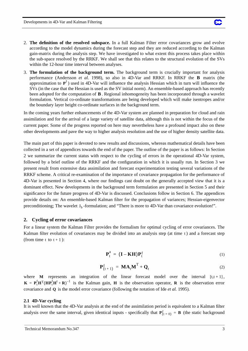
by initial-time energy singular vectors. Geopotential heights at 500hPa are modified by several metres (i.e bylarge fractions of typical observation and background errors which both are less than 10 m). Fig 11 shows across section of the difference in analysed temperature for the same date taken along the line 50N, 135E to40N, 175E. Clearly, the lack of impact on mean forecast scores is not simply due to a lack of impact on theanalysis.

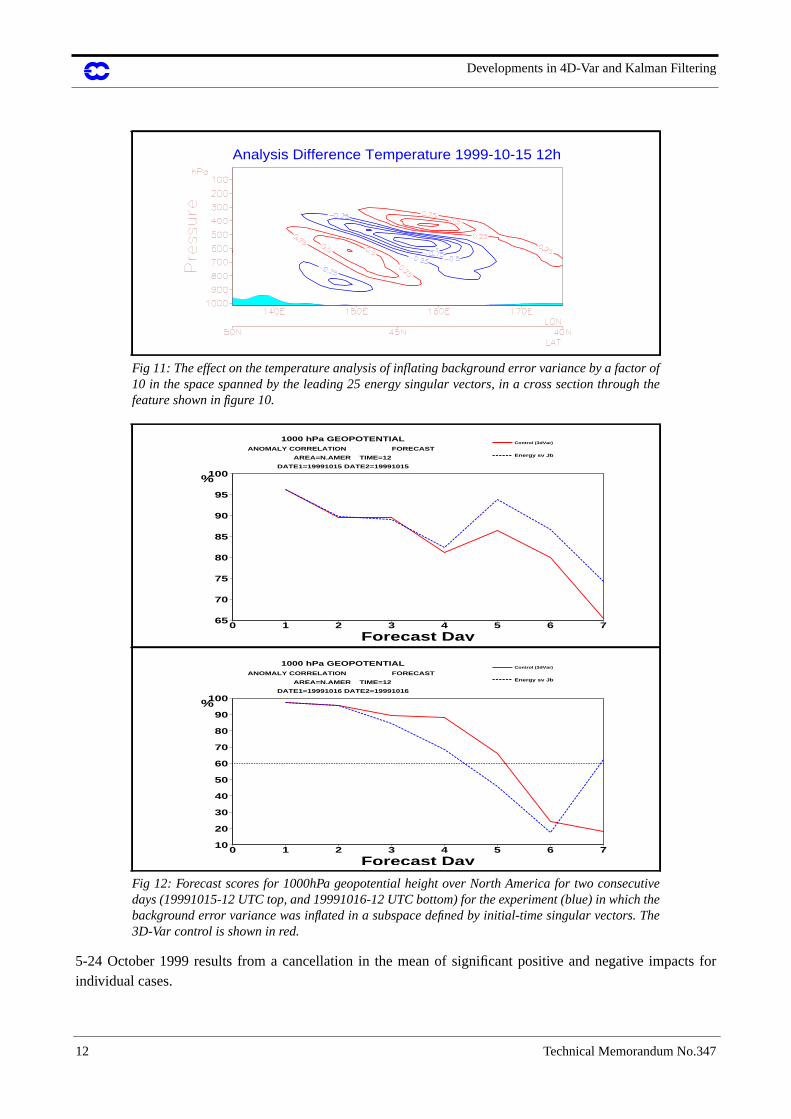
The forecast score for 1000hPa geopotential height over North America is shown for two consecutive dates infigure 12. The upper panel corresponds to forecasts run from the analyses whose difference is shown in figure10. There is a positive impact of the analysis difference on the forecast score. By contrast, the lower panelshows a negative impact, for the subsequent date. It seems that the neutral mean forecast score for the period

Fig 9: Northern Hemisphere forecast scores showing the effect of inflating background error inspaces defined by initial-time energy singular vectors (blue), evolved singular vectors (green) andthe 3D-Var control (red).

Fig 10: The effect on the 500hPa height analysis (19991015-12 UTC) of inflating background errorvariance by a factor of 10 in the space spanned by the leading 25 energy singular vectors. Thecontour interval is 2m. Negative analysis differences are shown in blue and positive in red.

0 1 2 3 4 5 6 7

Forecast Day50

55

60

65

70

75

80

85

90

95

100% DATE1=19991015/... DATE2=19991015/... DATE3=19991015/...




FORECAST VERIFICATIONControl (3dVar)

Energy sv Jb

Evol esv Jb

10 ON10O N

180O160OW140OW

120OW

100OW 100OE

120OE

140OE160OE

Analysis Difference 500hPa height (metres) 1999-10-15 12h



5-24 October 1999 results from a cancellation in the mean of significant positive and negative impacts forindividual cases.

Fig 11: The effect on the temperature analysis of inflating background error variance by a factor of10 in the space spanned by the leading 25 energy singular vectors, in a cross section through thefeature shown in figure 10.

Fig 12: Forecast scores for 1000hPa geopotential height over North America for two consecutivedays (19991015-12 UTC top, and 19991016-12 UTC bottom) for the experiment (blue) in which thebackground error variance was inflated in a subspace defined by initial-time singular vectors. The3D-Var control is shown in red.

Analysis Difference Temperature 1999-10-15 12h

0 1 2 3 4 5 6 7

Forecast Day65

70

75

80

85

90

95

100% DATE1=19991015 DATE2=19991015

AREA=N.AMER TIME=12


1000 hPa GEOPOTENTIALControl (3dVar)

Energy sv Jb

0 1 2 3 4 5 6 7

Forecast Day10

20

30

40

50

60

70

80

90

100% DATE1=19991016 DATE2=19991016

AREA=N.AMER TIME=12




Control (3dVar)

Energy sv Jb



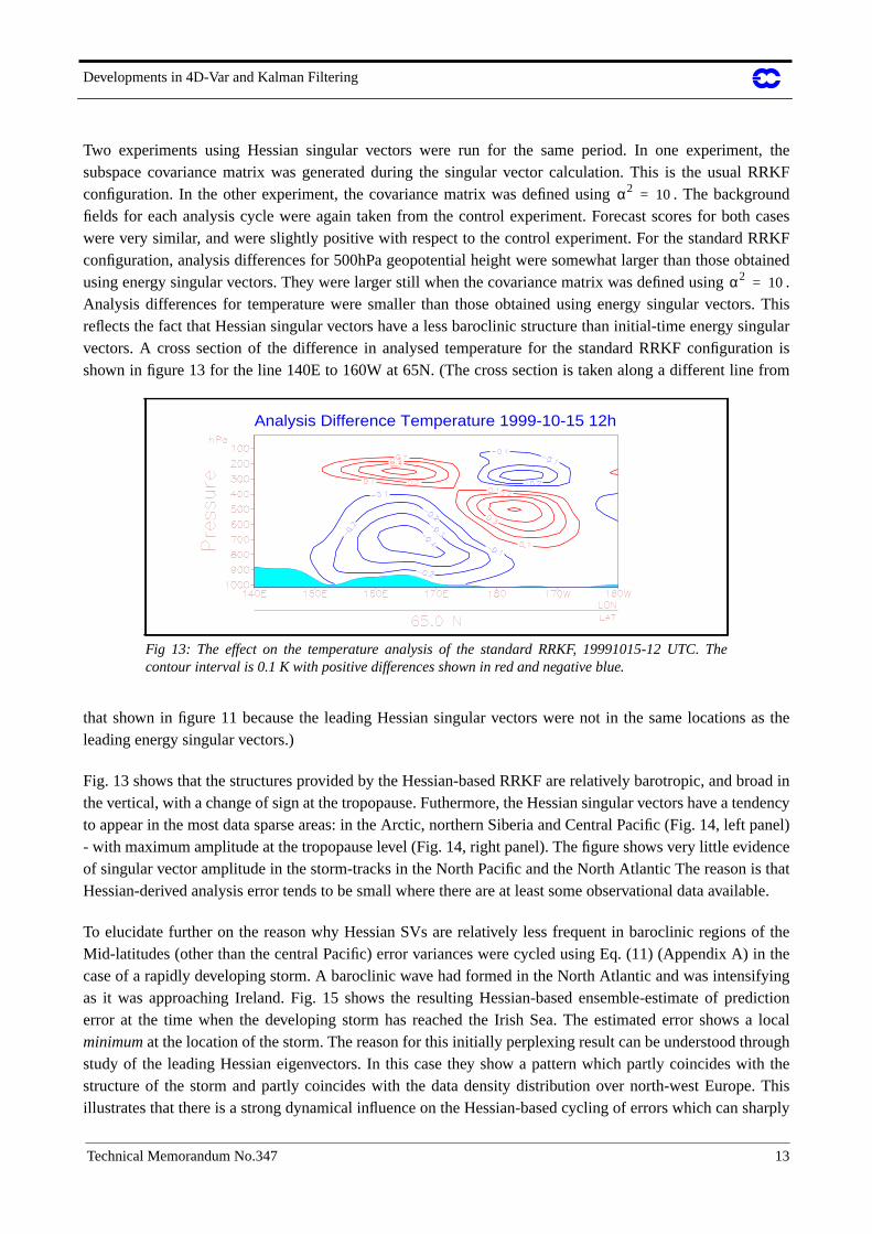
Two experiments using Hessian singular vectors were run for the same period. In one experiment, thesubspace covariance matrix was generated during the singular vector calculation. This is the usual RRKFconfiguration. In the other experiment, the covariance matrix was defined using . The backgroundfields for each analysis cycle were again taken from the control experiment. Forecast scores for both caseswere very similar, and were slightly positive with respect to the control experiment. For the standard RRKFconfiguration, analysis differences for 500hPa geopotential height were somewhat larger than those obtainedusing energy singular vectors. They were larger still when the covariance matrix was defined using .Analysis differences for temperature were smaller than those obtained using energy singular vectors. Thisreflects the fact that Hessian singular vectors have a less baroclinic structure than initial-time energy singularvectors. A cross section of the difference in analysed temperature for the standard RRKF configuration isshown in figure 13 for the line 140E to 160W at 65N. (The cross section is taken along a different line from

that shown in figure 11 because the leading Hessian singular vectors were not in the same locations as theleading energy singular vectors.)

Fig. 13 shows that the structures provided by the Hessian-based RRKF are relatively barotropic, and broad inthe vertical, with a change of sign at the tropopause. Futhermore, the Hessian singular vectors have a tendencyto appear in the most data sparse areas: in the Arctic, northern Siberia and Central Pacific (Fig. 14, left panel)- with maximum amplitude at the tropopause level (Fig. 14, right panel). The figure shows very little evidenceof singular vector amplitude in the storm-tracks in the North Pacific and the North Atlantic The reason is thatHessian-derived analysis error tends to be small where there are at least some observational data available.

To elucidate further on the reason why Hessian SVs are relatively less frequent in baroclinic regions of theMid-latitudes (other than the central Pacific) error variances were cycled using Eq. (11) (Appendix A) in thecase of a rapidly developing storm. A baroclinic wave had formed in the North Atlantic and was intensifyingas it was approaching Ireland. Fig. 15 shows the resulting Hessian-based ensemble-estimate of predictionerror at the time when the developing storm has reached the Irish Sea. The estimated error shows a localminimum at the location of the storm. The reason for this initially perplexing result can be understood throughstudy of the leading Hessian eigenvectors. In this case they show a pattern which partly coincides with thestructure of the storm and partly coincides with the data density distribution over north-west Europe. Thisillustrates that there is a strong dynamical influence on the Hessian-based cycling of errors which can sharply

Fig 13: The effect on the temperature analysis of the standard RRKF, 19991015-12 UTC. Thecontour interval is 0.1 K with positive differences shown in red and negative blue.

α2 10=

α2 10=

Analysis Difference Temperature 1999-10-15 12h



decrease the analysis error of the dynamically most active features in the analysis, where there is good datacoverage.

An experiment was conducted in which the subspace consisted of the single vector dubbed the “key analysiserror” by Klinker et al. (1998). That is, the direction was defined by a truncated minimization of 2-dayforecast error with respect to the initial conditions and an energy inner product. The RRKF analysis with thissubspace was essentially unmodified compared with the control analysis. Analysis differences were large-scale patterns with an amplitude of a few tenths of a metre. This is in marked contrast to the experimentswhich defined the unstable subspace using singular vectors. A further experiment was run in which thevariances were inflated by a factor of , and the number of iterations of minimization was doubled tocompensate for the resulting degradation in the numerical conditioning of the minimization problem. This toohad little impact on the analysis.

The inability of the analysis to draw in the direction of the “key analysis error” casts serious doubt on theinterpretation of this pattern as an analysis error. However, it does not rule out the possibility that in localizedregions the perturbation may coincide with analysis error, but with different amplitudes and signs in differentgeographical regions, and with the addition of decaying structures which may have little to do with analysis

Fig 14: Change in effective background error standard deviations (diagnosed using therandomisation method, Appendix A). Polar map (left) and zonal mean cross section (right).

Fig 15: Flow dependent cycling of error variances for 20001029-15 UT +12h using the method inAppendix A. The panel on the left shows 1000 hPa geopotential (contoured) and the correspondingestimated 12-hour prediction error, colour shaded from yellow (2-4m) to blue (13-14m), in steps of2m. The panel on the right shows the leading Hessian eigenvector, propagated by 12 hours.

α2 100=



error. The degree to which perturbations based on sensitivity calculations represent analysis error is an areawhich has received insufficient attention, but which has important implications for the RRKF. We intend toaddress this question in the near future.

3.3 DiscussionWe have seen that the RRKF in its current form does not have a significant overall impact on forecast scores,on average over large samples. This is true both of the original Hessian-based formulation and the severalvariations described above. This is surprising because the RRKF specifically modifies the analysis insensitive, unstable regions (as shown in Fig. 8 and Fig. 10). It is also contrary to the usual experience thatchanges to the formulation of the background error covariance matrix tend to have large effects on theaccuracy of the analyses and on forecast skill.

The interpretation of the results is difficult. One possibility is that the actual analysis error has little projectionon the unstable subspaces we have tried so far. For example, the actual analysis errors may initially have verysmall amplitude in the directions of the leading initial-time Hessian singular vectors, so that it is not until theyhave grown to several times their initial magnitude that they can be observed by the existing observingnetwork. By this time, their structure will no longer correspond to that of the initial-time singular vectors.

The neutral result can also be interpreted as an indication that both the energy and the Hessian initial normsare poor approximations of the actual analysis error covariance, to the extent that the RRKF subspace isunsuccessful in describing a substantial part of thelikely short-range forecast error evolution. Improvementsin the characterisation of analysis error and alternatives to the standard singular vector approach will beexplored in future work. We have seen that Hessian singular vectors tend to appear in those areas that are leastwell observed (the Arctic, northern Siberia and central North Pacific), i.e. where the estimated analysis error islarge and approximately equal to the background error. The spatial structure of the Hessian singular vectors inthose regions is therefore predominantly determined by the static , which favours isotropic and barotropicstructures of certain horizontal and vertical scales. The RRKF to date has not been able to pin-point the mostrelevant (often small scale and tilted) components of analysis error which experience tells us may occuranywhere in the baroclinic areas at mid-latitudes. A further possible explanation is that covariance evolution isless important than we have hitherto supposed. This is the topic of the next section.

4. Covariance evolution

The significantly better performance of 4D-Var compared with 3D-Var is widely attributed to the implicit usein 4D-Var of an evolving, flow-dependent covariance matrix of background error. There is, however, analternative explanation for the improvement, as will be explained in the following.

4.1 A first-order contribution to analysis errorConsider the 4D-Var cost function:

(5)

where, for convenience of notation, the vector is taken to include all the observations used in the analysis,and the observation operator includes the model integrations required to propagate the initial model stateto the times of the observations. The analysis is given by setting the gradient of the cost function to zero:

B

J x xb–( )TB 1– x xb–( ) y Hx–( )TR 1– y Hx–( )+=

y

H x



(6)

Let us define the true state as , and the true values of the observed quantities as . We will assume that theobservation error and the background error are unbiased, and seek an expression for the analysis error

. Straightforward substitution into equation 6 gives the following:

(7)

Taking the expectation of equation 7, the last term vanishes, and we arrive after a little rearrangement at:

(8)

Both 3D-Var and 4D-Var tacitly assume that , so that the expected analysis error is zero. However,this assumption is likely to be much more accurate in 4D-Var than in 3D-Var due to the inclusion in of thepropagation by the model of the initial state to the time of the observation. As a consequence, the expectederror of a 4D-Var analysis is likely to be smaller than that of a 3D-Var analysis.

The presence in 3D-Var of a mean analysis error means that we cannot unequivocally assign the betterperformance of 4D-Var to its supposedly better covariance statistics. To further emphasize this point, wepresent in Appendix D a simple theoretical example for which the covariance matrices of analysis error for3D-Var and 4D-Var areidentical, but for which 4D-Var is nevertheless demonstrably more accurate than 3D-Var.

Bouttier (personal communication) noted that, for a linear model and observation operators, the mean analysiserror given by equation 8 vanishes for the variant of 3D-Var known as 3D-FGAT. This is an incrementalalgorithm which replacesHx in equation 5 byH(xb)+H(x-xb), and retains the propagation of the initial stateby the model to the time of the observations inH, but not inH. 3D-FGAT has been shown to be superior to3D-Var, and for this reason is being used for the ECMWF 40-year re-analysis (ERA-40). This suggests thatelimination of mean error may indeed be an important factor in explaining the superiority of 4D-Var over 3D-Var.

The absence of a mean analysis error in 3D-FGAT does not imply that the better performance of 4D-Var isnecessarily due to improved covariance statistics. To see this, we rewrite equation 6 in a form which applies toboth 4D-Var and 3D-FGAT:

We see that, in 4D-Var, the analysis increment (xa-xb) is determined by two separate flow-dependent effects.First, the scaled observation departure is propagated back in time to the start of the analysiswindow by the action ofHT. This propagated departure is then acted on by the flow-dependent analysis errorcovariance matrix, . In 3D-FGAT, neither of these flow-dependent effects occurs,sinceH does not contain the tangent linear model dynamics.

xa B 1– HTR 1– H+( )1–

B 1– xb HTR 1– y+( )=

x* y*

εo εb

εa

εa x*– B 1– HTR 1– H+( )1–

B 1– x* HTR 1– y*+( )

B 1– HTR 1– H+( )1–

B 1– εb HTR 1– εo+( )

+

+

=

εa⟨ ⟩ B 1– HTR 1– H+( )1–HTR 1– y* Hx*–( )=

y* Hx*=

H

xa xb B 1– HTR 1– H+( )1–HTR 1– y H xb( )–( )+=

R 1– y H xb( )–( )

Pa B 1– HTR 1– H+( )1–

=



In general, it is difficult to determine which of the two flow-dependent effects is dominant in 4D-Var.However, in the example given in Appendix D it is trivial to separate them, since the example is explicitlyconstructed so that, even in 4D-Var, the analysis error covariance matrix is not flow-dependent. In this case,the demonstrable advantage of 4D-Var over 3D-FGAT comes purely from the action ofHT in propagating thebackground departure to the start of the analysis window. In the next section we present an experiment whichsuggests that this is also the dominant flow-dependent effect in the full ECMWF 4D-Var analysis.

The improved performance, at LT511/T159 resolution (see Appendix B), of 12h 4D-Var compared with 6h4D-Var provides a counter-argument to the hypothesis that covariance propagation may be relativelyunimportant in 4D-Var. Once again, we may appeal to mean analysis error to explain the difference. Thecurrent observing network contains important classes of observations which report at 12 hourly intervals. Thisclass includes large numbers of radiosondes. With a 6 hour analysis cycle, only alternate analyses containthese data. The intervening analyses do not. This leads to a 6 hour oscillation in the mean analysis error whichresults from biased observations. It was observed that this “flip-flop” effect was greatly reduced when 12h 4D-Var was introduced. Moreover, the largest impact of increasing the analysis cycle to 12 hours was over eastAsia, where the “flip-flop” effect is large. It is entirely possible that a reduction of analysis bias is sufficient toexplain the improved performance of 12h 4D-Var compared with 6h 4D-Var.

4.2 Extended window 4D-VarTo try to quantify the importance of covariance propagation in 4D-Var, we ran a 12h 4D-Var analysisexperiment in which the initial time of the analysis window was moved back in time by 9 hours. We call thissystem “extended-window 4D-Var”. No observations were assimilated during the initial 9 hours of eachassimilation window, so that the observation cost function was identical to that of the usual 12h 4D-Var.Background fields were taken from the appropriate time step of the preceding cycle’s 4D-Var analysis. Notethat, since a 4D-Var analysis is a model trajectory, the background trajectory for extended-window 4D-Var isno less accurate than in a normal 12h 4D-Var analysis. (In practice, the 4D-Var analysis is not exactly a modeltrajectory due to the way in which the surface fields are analysed. Also, the low resolution trajectory whichprovides the linearization state for the tangent linear and adjoint models during the minimization may besomewhat less accurate than for a normal 12h 4D-Var. Neither of these effects are thought to have had asignificant impact on the performance of the extended-window analysis system.)

At the start of the analysis window, the background error covariance matrix in a 4D-Var analysis is equal tothe static covariance matrix specified in the background cost function. This covariance matrix is thenimplicitly propagated forward in time according to the tangent linear dynamics to generate flow-dependent“structure functions” at later times during the assimilation window. In the extended-window analysis, thebackground error covariance matrix is propagated over an additional 9 hours. Except for minor differencesdue to the surface analysis and the accuracy of the low resolution linearization trajectory, the additionalcovariance evolution is the only difference between extended-window 4D-Var and the conventional 4D-Varanalysis. Fig. 16 illustrates extended-window 4D-Var schematically. Note in particular that covarianceevolution effectively takes place in the entire control space. Thus, the extended-window analysis sidestepsquestions about the choice of subspace to be propagated and the choice of inner product with which to defineprojection onto the subspace.

Three analysis experiments were conducted with the extended-window system. These corresponded todifferent specifications of the static covariance matrix at the start of the analysis window. In the first



experiment, the matrix was the same as is used in 12h 4D-Var. In the second experiment, the matrix wasmultiplied by a factor of 0.84 to account approximately for the growth of forecast error variance over 9 hours.In the third experiment, the structure of the matrix was kept the same, but the statistics were calculatedfrom differences between analyses from an ensemble of analyses. In other words, the covariance matrix was astatic model of analysis error. Mean forecast scores for these experiments are shown in Fig. 17. There isessentially no impact of extending the analysis window, which demonstrates that covariance evolution maynot be the dominating effect that determines 4D-Var performance.

5. Developments in 4D-Var

The discussions in Section 3.3 emphasised the importance of the static matrix in its influence on the 4D-VarHessian, and therefore also on the RRKF. Improvements to the -formulation are of great significance to theperformance of 4D-Var (e.g. Derber and Bouttier 1999), and its continued development has remained apriority.

Fig 16: Schematic representation of extended window 4D-Var. The analysis cycle which producesthe 0z analysis (bottom) takes its background fields from the 6z analysis of the preceding cycle(top). However, as in a normal 12h 4D-Var analysis, observations are assimilated only during the12h period from 15z to 3z.

Fig 17: Northern Hemisphere forecast scores for extended-window 4D-Var.

3z 15z12z

0z 3z

0z18zObs

Obs

6z

Background fields

6z Analysis

B B

B

0 1 2 3 4 5 6 7

Forecast Day55

60

65

70

75

80

85

90

95

100% DATE1=20000913/... DATE2=20000913/... DATE3=20000913/... DATE4=20000913/...




FORECAST VERIFICATIONControl

Long Window 0.59

Long Window 0.70

Long Window Ja

B

Jb



5.1 Background error formulationVariational background terms are commonly formulated in spectral space for reasons of computationalefficiency. Isotropic and homogeneous covariances are spectrally represented simply by a diagonal matrix.Non-separability between horizontal and vertical scales can also be incorporated relatively easily (Courtieretal. 1998). However, Anderssonet al. (1998) found that the very significant advantages of non-separability (in3D-Var) were largely offset by equally significant disadvantages due to the poor representation of the regionalvariations of background error statistics (in comparisons with an Optimum Interpolation scheme with a grid-point ). Current -formulation (Derber and Bouttier 1999) allows some latitudinal variation in temperature(but not vorticity) background error statistics through its varying mass/wind coupling.

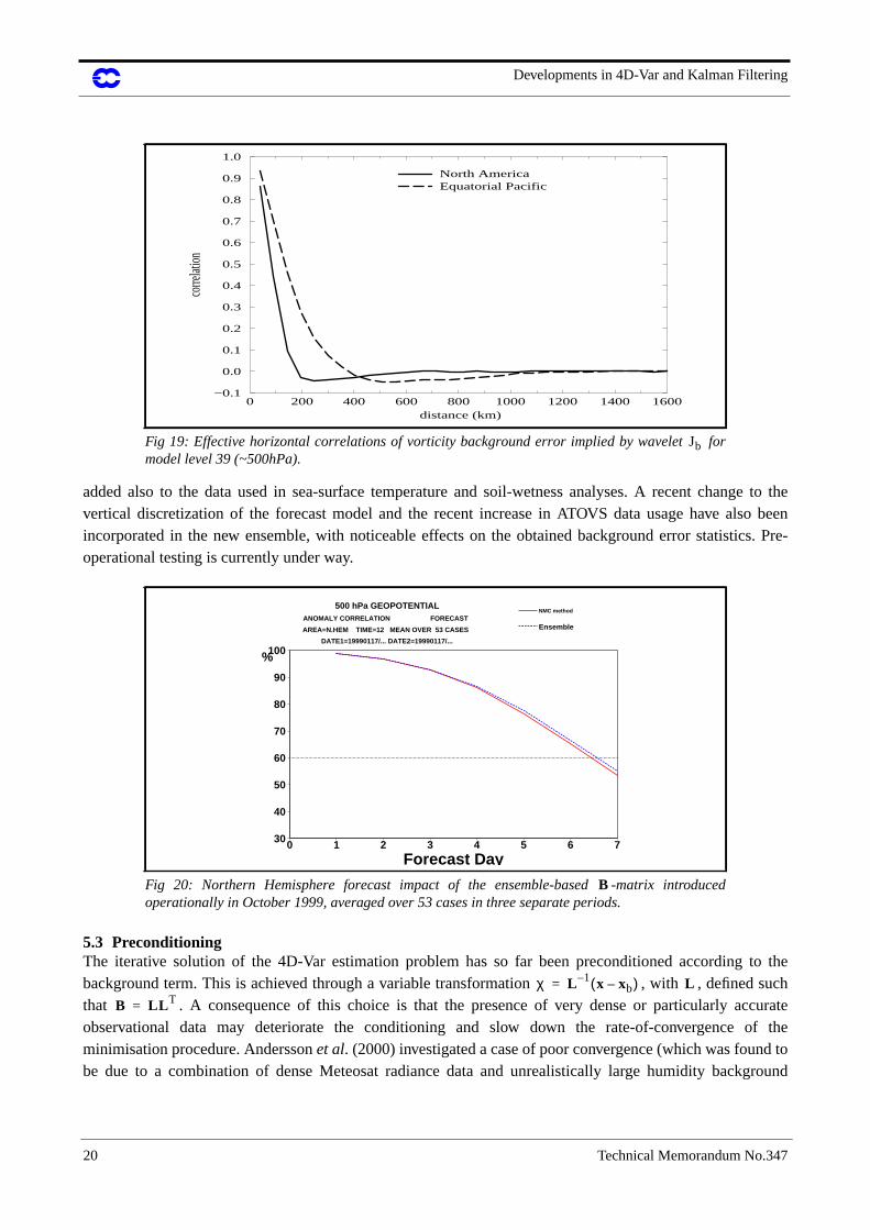
The wavelet- described in Appendix C allows the advantages of non-separability to be combined with adegree of regional variation in the statistics. Fig. 18 shows the effective wavenumber-averaged verticalcorrelation matrix for vorticity background error implied by the wavelet for points in North America andover the Equatorial Pacific. The differences between the two diagrams reflect differences in tropopause heightand boundary layer depth in the two regions. Fig. 19 shows the horizontal correlation of background error forvorticity implied by the wavelet for North America and for the Equatorial Pacific. The wavelet producessignificantly more large-scale correlations in the equatorial region (dashed line) than in North America (fullline). The latitudinal variation in horizontal length scales is a prevalent feature in background error statistics(Ingleby 2001) which (for vorticity) has so far been neglected in ECMWF’s 3D and 4D-Var.

5.2 Calculation of statisticsA new method for the calculation of background error statistics has been developed. It relies on an ensembleof data assimilation experiments, in which the members differ because of random noise added to theobservations, in accordance with the assumed observation errors. A detailed description of the method with acompilation of results is currently in preparation. The main feature of the ensemble statistics is that vertical aswell as horizontal length-scales are reduced, compared to statistics based on lagged forecast differences (the“NMC-method”). A -matrix based on a 3D-Var ensemble was implemented in operations (version labelled21r4) in October 1999. There was an important beneficial forecast impact associated with this change, asshown in Fig. 20. A second ensemble has recently been completed, this time using 4D-Var, with perturbations

Fig 18: Effective wavenumber-averaged vertical correlation matrices for vorticity for wavelet .The panel on the left shows North America, and Equatorial Pacific is on the right. Model level30=202 hPa, 45=728 hPa and 50=884 hPa.

B

B Jb

Jb

Jb

Jb Jb

10 20 30 40 50 60

model level

60

50

40

30

20

10

mod

el le

vel

average vorticity cors

0.2

0.2

0.4

0.4

0.6

0.6

0.8

0.8

10 20 30 40 50 60

model level

60

50

40

30

20

10

mod

el le

vel

average vorticity cors

0.2

0.2

0.4

0.4

0.6

0.6

0.8

0.8

Jb

Jb

B



added also to the data used in sea-surface temperature and soil-wetness analyses. A recent change to thevertical discretization of the forecast model and the recent increase in ATOVS data usage have also beenincorporated in the new ensemble, with noticeable effects on the obtained background error statistics. Pre-operational testing is currently under way.

5.3 PreconditioningThe iterative solution of the 4D-Var estimation problem has so far been preconditioned according to thebackground term. This is achieved through a variable transformation , with , defined suchthat . A consequence of this choice is that the presence of very dense or particularly accurateobservational data may deteriorate the conditioning and slow down the rate-of-convergence of theminimisation procedure. Anderssonet al. (2000) investigated a case of poor convergence (which was found tobe due to a combination of dense Meteosat radiance data and unrealistically large humidity background

Fig 19: Effective horizontal correlations of vorticity background error implied by wavelet formodel level 39 (~500hPa).

Fig 20: Northern Hemisphere forecast impact of the ensemble-based -matrix introducedoperationally in October 1999, averaged over 53 cases in three separate periods.

0 200 400 600 800 1000 1200 1400 1600 distance (km)

−0.1

0.0

0.1

0.2

0.3

0.4

0.5

0.6

0.7

0.8

0.9

1.0

cor

relat

ion

North AmericaEquatorial Pacific

Jb

0 1 2 3 4 5 6 7

Forecast Day30

40

50

60

70

80

90

100% DATE1=19990117/... DATE2=19990117/...





NMC method

Ensemble

B

χ L 1– x xb–( )= L

B LLT=



errors) and derived an expression for the 4D-Var condition number as a function of data density and thebackground-to-observation error ratio.

More recently, in experiments with additional AMSU-A data, the data coverage in the Arctic stratosphere,where orbits overlap, became excessively dense so that conditioning, and thus the rate-of-convergence, wereseverely affected. A solution to these difficulties has now been provided through the Hessian eigenvectorpreconditioning presented in Appendix B. It is expected that this new feature will be highly relevant for thesuccessful assimilation of future high-density satellite data.

The new preconditioning procedure makes the 4D-Var algorithm significantly more efficient, and is alreadybenefiting the 40-year re-analysis (ERA-40). Its effect on the cost function and gradient reduction during theminimisation is illustrated in Fig. 21.

6. Conclusions

We have presented results showing that the RRKF, as currently formulated, has an entirely neutral impact onforecast scores. Moreover, this result is insensitive to the dimension of the resolved unstable subspace, and tochanges in the subspace produced by varying the optimization time or the initial inner product used in thesingular vector calculation. The neutral result can be interpreted as an indication that both the energy and theHessian initial norms are poor approximations of the actual analysis error covariance, to the extent that theRRKF subspace is unsuccessful in describing a substantial part of the fast-growing short-range forecast errorsin the assimilation. Attempts to use so-called “key analysis error” perturbations to define the analysissubspace cast doubt on the interpretation of these perturbations as analysis errors. Experiments usingextended-window 4D-Var cast doubt on the conventional explanation that 4D-Var’s superior performance(relative to 3D-Var) results from its implicit dynamical propagation of error covariance.

Fig 21: Cost function (left) and its gradient norm (right) as a function of the iteration count, duringminimisation using the M1QN3 optimization algorithm (Gilbert & Lemarechal, 1989). The exampleis taken from the 40-year re-analysis (ERA-40) which uses 3D-Var. The benefit of Hessian eigen-vector preconditioning (red lines) compared to -preconditioning (black) is clear from the fasterdecrease in cost function and by the steeper reduction in gradient norm.

0.0 20.0 40.0 60.0 80.0Iteration

1.5e+05

2.0e+05

2.5e+05

3.0e+05

3.5e+05

4.0e+05

Hessian Eigenvector PreconditioningERA 40

0018 (control)0242 (preconditioned)

0.0 20.0 40.0 60.0 80.0Iteration

100

102

104

106

108

Squ

are

of G

radi

ent N

orm

Hessian Eigenvector PreconditioningERA 40

0018 (control)0242 (preconditioned)

Jb



6.1 Comments on the future development of 4D-VarThe work on preconditioning as well as RRKF make extensive use of the 4D-Var Hessian. Recent study of theleading Hessian eigenvectors has provided four results of strategic importance for the continued developmentof 4D-Var:

• They are relatively large scale. We can therefore be confident that further increases of inner-loop resolu-tion can be achieved without deteriorating the conditioning of the problem. An inner-loop resolution ofT399 is envisaged within the next four years, or so.

• They reflect high data density. Appropriate Hessian pre-conditioning will therefore be a required ingre-dient for the successful assimilation of future high-density satellite data in the coming years. Issues relat-ing to the information content in new data types will require further study. This will include channelselection, data thinning and modelling of observation error correlations .

• They are modulated by the tangent-linear physics. It is therefore expected that further improvements inthe linearization of physical processes (Janiskova, 2001) will be valuable for the data assimilation per-formance. More extensive use of the linearized physics within 4D-Var will be exploited, when the compu-tational resources required become available in 2003.

• They are influenced by the model dynamics (through covariance propagation) and by the static back-ground error covariances. This confirms that the -term remains crucially important also with 12-hourlycycling. Continued development of the formulation and relatively frequent re-calibrations of the statis-tics will take place.

6.2 The future of the RRKFWe have hypothesized that covariance evolution may be less important than expected in explaining thesuperiority of 4D-Var over 3D-Var. This does not necessarily imply that a well-formulated Kalman filter willnot bring substantial improvements in the accuracy of the analysis (although it is clearly now a priority toquantify the potential benefits). Instead, it may indicate that we are attempting to propagate an approximatecovariance matrix of analysis error which is such a poor approximation to the true covariance matrix that thepropagated matrix is a no more realistic representation of forecast error covariance than the static matrix.Pertinent to this suggestion is the question of the overlap of initial and partially evolved Hessian singularvector subspaces.

At each analysis cycle of the RRKF, the Hessian singular vector calculation implicitly propagates theprojection of the analysis error covariance matrix onto initial-time singular vectors. The propagatedcovariance matrix valid 12 hours later forms the background error covariance matrix for the unstablesubspace. This subspace is defined by the 12-hour-evolved singular vectors. Covariances of background errorfor directions orthogonal to the subspace are provided by the static matrix.

Leutbecher has shown (personal communication) that the projection of 12-hour-evolved Hessian singularvectors onto initial-time singular vectors is rather small (less than 30%). This implies that much of the flow-dependent covariance information contained in the analysis Hessian at a given cycle of analysis is notpropagated to the next cycle, since this information is known only for a space which is nearly orthogonal tothe initial-time singular vectors. As a consequence, it is largely the static covariance information which ispropagated. A recent paper by Reynoldset al. (2001) explains (their figure 16) that this lack of overlap is dueto a phase difference between the evolved singular vectors (which propagate with the group velocity) and theinitial-time singular vectors (which tend to follow the individual developing storm systems, i.e. the phase-

R

JbJb

B

B



speed). Extended-window 4D-Var demonstrates that there is no benefit to forecast skill in propagating a staticapproximation to the covariance matrix.

Recently, a new type of subspace based on Hankel singular vectors, has been proposed by Farrell and Ioannou(2001a; 2001b). Their subspace balances, in an optimal way, the initial perturbations and the evolvedresponses of the forecast model. In effect, the projection of the initial covariance matrix of analysis errorremains largely within the subspace as it evolves. By using this approach, we expect that the subspaces used atsuccessive analysis cycles would overlap significantly, so that flow-dependent covariance information wouldbe propagated from one cycle to the next.

We propose a two-pronged attack. The first objective will be to quantify, in a reasonably realistic environment,the benefits which should be expected from a Kalman filter. To do this, we will collaborate with DrEhrendorfer of the University of Vienna, who will compare full and reduced-rank Kalman filters with 4D-Varin a T21 3-level quasi-geostrophic system. Observations will be taken from a “truth run” of the quasi-geostrophic model, so that analysis errors may be quantified exactly. The second line of attack will be toevaluate the use of approximate Hankel singular vectors to define the subspace in which covarianceinformation is evolved.

AcknowledgementsWe are grateful to the members of the Data Assimilation section for their contributions towards thedevelopments presented here, and to Anthony Hollingsworth, Adrian Simmons, Tim Palmer, FrancoisBouttier, Jan Barkmeijer and Martin Leutbecher for in-depth discussions of the results. We thank Els Kooij-Connally for editing and formatting the manuscript.



Appendix A An ensemble-based Kalman filter for the propagation of variancesFollowing suggestions by Fisher and Courtier (1995) the analysis error covariance is estimated using thecombined Lanczos/conjugate gradient algorithm which finds approximately the leading eigenvectors ofthe 4D-Var Hessian and the associated eigenvalues . The leading eigenvectors describe the directions incontrol-vector space in which the information from observations is most important. By applying the change ofvariable operator to each eigenvector, an estimate of the analysis error covariance in model space isobtained:

(9)

where is the number of computed eigenvectors. Only the variances, i.e. the diagonal elements of , arecomputed.

The randomisation method. A randomisation method can be used to calculate a low-rank estimate of , interms of model variables (Fisher and Courtier 1995). In particular the diagonal of can be estimated by

(10)

where is a set of random vectors in control-vector space, drawn from a population with zero mean andunit Gaussian variance. Variances produced by randomisation are somewhat noisy. The amplitude of the noisedecreases as is increased.

Propagation in time. The simple error growth model of Savijärvi (1995) used so far in 4D-Var representsexponential error growth of small errors and the asymptotic behaviour of large errors towards a climatologicalvariance (Fisher 1996). It lacks the dynamical i.e. flow-dependent effects on error growth. From Kalman Filtertheory (Eq. (2)) we have an expression for the evolution of the prediction error covariance matrix,

, where is the tangent linear of the forecast model and is the model errorcovariance. Inserting the approximate forms for and from Eq. (9) and Eq. (10) into Eq. (2), we have:

(11)

Eq. (11) provides an expression for the evolution of error variances to any future time within the range ofvalidity of the tangent linear approximation. In the current operational context around 90 -vectors arecomputed. By setting the additional cost is 90+50=140 12-hour integrations of the adiabatic tangentlinear model , at low resolution (e.g. TL95). It is hoped that this method could replace the current simpleerror-growth model and introduce the previously lacking flow-dependent effects on error growth. The viabilityof the method has been demonstrated by Andersson and Fisher (1999), where example illustrations can alsobe found.

Pa

νkλk

A

A B λk1–

1–( ) Lνk( ) Lνk( )T

k 1=

M

∑+=

M A

BB

B1N---- Lξ i( ) Lξ i( )T

i 1=

N

∑≈

ξ i N

N

Pf

MAMT

Q+= M QA B

Pf 1N---- MLξ i( ) MLξ i( )T

i 1=

N

∑ λk1–

1–( ) MLνk( ) MLνk( )T

k 1=

M

∑+≈

νkN 50=

M



Appendix B Hessian-Eigenvector PreconditioningThe exact rate of convergence of the minimization in 4D-Var depends in a complicated way on the details ofthe algorithm used and on the distribution of the eigenvalues of the Hessian matrix of the analysis costfunction. Fisher (1998b) shows that for a quadratic cost function and conjugate gradient minimization, thefollowing upper bound provides a good estimate of the actual convergence rate in the ECMWF analysis:

. (12)

Here, is a measure of the error remaining in the solution after n iterations of minimization, and isthe condition number (i.e. the ratio of the largest to the smallest eigenvalue) of the Hessian. By expanding thisexpression as a power series in , and truncating to first order, we arrive at an estimate of the number ofiterations of minimization required to reduce the Hessian-norm of the error by a factor :

(13)

(Currently, the cost function in the ECMWF analysis is not quadratic, and the quasi-Newton minimizationalgorithm M1QN3 (Gilbert and Lemarechal, 1989) is used. As a consequence, the number of iterationsrequired to achieve a given error reduction is roughly twice the estimate given above.)

Consider a general inner product , defined by:

(14)

where is a positive-definite symmetric matrix.

Expressing the analysis cost function as a Taylor expansion with respect to this inner product, we have:

(15)

Both the gradient and the Hessian are dependent on the choice of inner product. In particular, the Hessian withrespect to the P-inner product is related to the Hessian with respect to the Euclidean inner product, , via:

(16)

The quasi-Newton minimization algorithm M1QN3 allows the user to precondition the minimization byspecifying the inner product to be used during the minimization. The optimal choice is , since theHessian with respect to the P-inner product is then the identity matrix, which has the smallest possiblecondition number of one. However, it is not possible to use the Hessian matrix itself as a preconditioner, sincethe minimization algorithm requires that is easily inverted. We therefore choose an approximation to theHessian.

Fisher and Courtier (1995) show that an approximation to the Hessian of the cost function may be constructedfrom its leading eigenvalues and eigenvectors, and . This approximation is already used in the analysis

e n( )J″2

2κ 1–

κ 1+----------------

n

e 0( )J″2

≤

e n( )J″2

κ

1 κ⁄ε

n12--- κ 2

ε---

ln≈

. .,⟨ ⟩ P

p q,⟨ ⟩ P pTPq=

P

J x0 δx+( ) J x0( ) δx JP∇,⟨ ⟩ P δx J″P δx,⟨ ⟩ O δx3( )+ + +=

J″2

J″P P 1–J″2=

P J″2=

P

λk vk



system to estimate the variances of analysis error. The leading eigenvalues and eigenvectors are determinedusing a Lanczos algorithm (Lanczos 1950). Moreover, since the leading eigenvectors are large-scale patterns,they may be determined accurately, but cheaply, at low horizontal resolution.

Hessian eigenvector preconditioning (Fisher and Courtier, 1995) defines the minimization inner product as:

(17)

Here, are the leading eigenvectors of . The coefficients have yet to be defined.

The inverse of is given by replacing by in equation 17. (This is a consequence of theorthonormality of the eigenvectors.) So, substituting for in equation 16, and replacing by its fulleigen-decomposition (with eigenvalues arranged in descending order) we have:

(18)

Using the orthonormality of the eigenvectors, this may be written as:

(19)

That is, the preconditioned Hessian has the same eigenvectors as the un-preconditioned Hessian , butthe leading eigenvalues are reduced by factors . By choosing these factors so that ,we produce a preconditioning which reduces the condition number of the Hessian by a factor . (Notethat the preconditioning effect is relatively insensitive to the precise choice of the parameters ,provided that they respect the bound . However, too-large values of may make thecomputations which use the preconditioner ill-conditioned and subject to excessive rounding error.)

Clearly, the effectiveness of the preconditioner increases monotonically with the number of vectors used.However, this must be offset against the computational cost of calculating, manipulating and storing theeigenvectors. The eigenvalue spectrum of the Hessian for the ECMWF analysis decreases rapidly for the firstfew eigenvalues, so that two or three eigenvectors are sufficient to reduce the condition number by a factor oftwo. However, the spectrum flattens out, so that typically around 25 vectors will reduce the condition numberby a factor of six or seven. In the ECMWF system 25 vectors represents a reasonable compromise betweeneffective preconditioning and the additional cost of manipulating the preconditioner. The factor of six or sevendecrease in the condition number corresponds to a decrease by a factor of roughly 2.5 in the number ofiterations of minimization required to achieve a given level of accuracy in the minimization. This has alsobeen demonstrated in practice as shown in Fig. 21.

P I µk 1–( )vkvkT

k 1=

K

∑+=

vk J″2 µk

P µk 1 µk⁄P 1– J″2

J″P I 1µk----- 1–

vkvkT

k 1=

K

∑+

λkvkvkT

k 1=

N

∑

=

J″Pλk

µk-----

vkvkT

k 1=

K

∑ λkvkvkT

k K 1+=

N

∑+=

J″P J″2K µ1…µK λk µk⁄ λK 1+<

λK 1+ λ1⁄µ1…µK

µk λk λK⁄> µ1…µK



Appendix C Wavelet FormulationIt is well known (Phillips 1986, Bartello and Mitchell 1992) that the vertical and horizontal scales ofbackground error covariance are non-separable: large horizontal scales tend to have deeper verticalcorrelations than small horizontal scales. It is essential to retain this property in the covariance model forbackground error in order to achieve a correct description of the covariance structures for both wind andtemperature (Rabieret al. 1998; Anderssonet al., 1998). Courtieret al. (1998), Derber and Bouttier (1999)achieve a non-separable model of background error covariance matrix by specifying different verticalcorrelation matrices for each total spherical wavenumber . However, for variables which are unmodified bythe balance operator (in particular, for vorticity), the covariance model is isotropic and homogeneous.

It is also well known that horizontal and vertical correlations vary geographically (Lönnberg 1988).Horizontal scales tend to be broader in the tropics than at high latitudes, as a consequence of atmosphericdynamics (Ingleby 2001). Correlation scales have also been shown to be influenced by variations in datadensity (Bouttier 1993).

Derber and Bouttier’s formulation (the current ) may be seen as one end of a spectrum. It allows fullresolution of the variation of vertical correlation with horizontal scale (as measured by ), but it allows nohorizontal variability of the vertical correlations. At the other end of the spectrum is the separable formulationwhich allows full horizontal variation of the vertical correlations (we may specify a different verticalcovariance matrix for each horizontal grid point), but has no variation of vertical correlation with horizontalscale. The wavelet achieves a compromise between these two extremes and allows a degree of variation ofvertical correlation with both wavenumber and horizontal location. Moreover, it also allows horizontalvariation of horizontal correlation.

The multivariate aspects of the wavelet are identical to those described by Derber and Bouttier (1999).Cross-correlations between mass and wind are described by a statistically-derived “balance operator” whichsubtracts from the temperature, log(surface pressure) and divergence, the components which can be explainedby the vorticity. The residual “unbalanced” fields, together with vorticity, specific humidity and ozone, aretreated univariately. The differences between the wavelet and the current formulation lie in the differenttreatment of these univariate covariances, which we now describe.

The wavelet is based on a wavelet expansion for the sphere. In recent years, there have been severalattempts to formulate such an expansion. Frequently, an orthogonal basis is sought. However, any suchorthogonal basis will necessarily manifest some form of “pole problem”, making it unattractive for use in aspectral model. Recently, Freeden and Windheuser (1996) have suggested defining spherical wavelets in termsof convolutions with radial basis functions (i.e. functions of great-circle distance, ). Such wavelets are freefrom “pole problems”, but are non-orthogonal.

Freeden and Windheuser’s idea is to generate wavelets from a family of bell-shaped radial basis functions. Freeden and Windheuser define the functions in terms of a single generator function. This has

advantages when considering infinite expansions of functions on the sphere, since it makes the waveletexpansion easier to handle mathematically. In the case of a finite wavelet expansion, this restriction is notnecessary. Instead, we may define a sequence of “cutoff” wavenumbers (with ) and require thatthe spectral transform of satisfy

Jb

n

Jb

n

Jb

Jb

Jb Jb

Jb

r

ϕ j r( )

Nj Nj Nj 1+<ϕ j r( )



(20)

The wavelets are defined in terms of as . Note that is zero outside that therange . So, convolution with results in a spectral bandpass filtering. Furthermore,

is itself a radial basis function which decays with great-circle distance. So, convolution withmay also be thought of as a localized spatial averaging. In other words, convolution with achieves thesimultaneous localization in space and wavenumber which is the hallmark of a wavelet transform.

The non-orthogonal wavelet expansion of a function on the sphere is defined as the set of functions(where denotes convolution). These functions have finite spectral truncations. They may

therefore be represented exactly on grids of appropriate resolution. The value of at a given grid point is alocalized spatial average of at nearby points.

An important property of the wavelet transform is that may be reconstructed from its transform by furtherconvolutions with :

(21)

This is easily proved by taking the spectral transform of the right hand side of equation 21:

(22)

The final sum collapses to leave only:

(23)

The result holds if we define and .

This property (equation 21) of the wavelet transform means that to reconstruct the function from itstransform , we apply localized spatial averaging to each of the functions before summing over . It is thisproperty which allows us to construct the wavelet .

The wavelet , like the current formulation, defines the background error covariance matrix implicitly viaa change of variable, . The minimization is carried out in terms of a control variable for which thebackground cost function is . The departures of model variables from the background are given by

. In the wavelet , the control vector is defined in the wavelet space as a set of functions , andthe background cost function is

(24)

ϕ̂ j n( ) 0= for n Nj>

ϕ̂ j n( ) 1= for n Nj 1–≤

ϕ̂ j n( ) ψ̂ j n( ) ϕ̂ j2 n( ) ϕ̂ j 1–

2 n( )–= ψ̂ j

Nj 1– n Nj 1+≤ ≤ ψ j r( )ψ j r( ) ψ j r( )

ψ j r( )

f λ θ,( )

f j f ψ j⊗= ⊗f j

f

f

ψ j r( )

f f j ψ j⊗j

∑=

f̂ j m n,( )ψ jˆ n( )

j∑ f̂ m n,( )ψ j

ˆ 2n( )

j∑

f̂ m n,( ) ϕ̂ j2

n( ) ϕ̂ j 1–2

n( )–( )j

∑

=

=

f̂ m n,( ) ϕ̂J2

n( ) ϕ̂02

n( )–( )

ϕ̂J n( ) 1 n∀= ϕ̂0 n( ) 0 n∀=

f

f̂ j f̂ j j

Jb

Jb Jb

L χJb

12---χ

Tχ=

x-xb Lχ= Jb χ j

Jb12--- χ j

Tχ jj

∑=



The univariate part of the change of variable consists of the following steps. First, each vertical column offor each is multiplied by the symmetric square-root of a square matrix whose columns havedimension equal to the number of levels. In principle, there is one such covariance matrix for each grid pointfor each . In practice, to reduce the computer memory required to store them, the matrices are stored oncoarser grids and interpolated to the grid points as needed.

Next, the functions are convolved with the wavelet functions and summed according toequation 21. The matrices account for both the vertical and horizontal correlations of backgrounderror. So, the reconstituted function must be multiplied by the standard deviations of background error, andoperated on by the balance operator to restore mass-wind cross-correlation. These last two steps of the changeof variable are identical to the corresponding steps of the current formulation.

It is convenient to write the change of variable in matrix form:

(25)

where is the balance operator and is the diagonal matrix of standard deviations of background error.Subscripts indicate the sequence of wavelet functions. For the wavelet function is broad and itsspectral transform is limited to the lowest wavenumbers. For , the wavelet function is narrow, and itsspectral transform is limited to the highest resolved wavenumbers. The matrices represent sphericaltransforms from the grid appropriate to the spectral truncation imposed by convolution with . Theconvolutions are represented by the matrices , which are diagonal (in spectral space). The matrices areblock diagonal with one block for each variable and for each horizontal grid point. These blocks are thematrices . The background error covariance matrix is given by . That is,

(26)

To understand the effect of the wavelet , we will consider the matrix represented by the sum (inparentheses) in equation 26, since the remainder of the matrix is identical to the current formulation. Wenote also that the current formulation corresponds to replacing the term in parentheses in equation 26 by ablock diagonal matrix whose blocks vary with total wavenumber. Each block in this formulation is amatrix , where is the vertical correlation matrix for each total wavenumber , and is adiagonal matrix whose elements are the modal variances at each level. ( defines the horizontal structurefunctions.)

For the wavelet , consider first the case in which the matrices are independent of latitude andlongitude. Then, commutes with the spherical transform, and we arrive at the following expression for thecorrelation between coefficients for different wavenumbers ( and ) and levels ( and ):

(27)

Note that the wavelet does not assume that different total wavenumbers are uncorrelated. For the particularcase , we have

χ j

j C j λ θ,( )

j

C j1 2⁄ λ θ,( )χ j ψ j r( )

C j λ θ,( )

Jb

L KSJΣbSJ1– Ψ0S0C0

1 2⁄ Ψ1S1C11 2⁄ … ΨJSJCJ

1 2⁄,,,( )=

K Σb

j j 0=

j J=

S j

ψ j r( )Ψ j C j

C j λ θ,( ) B LLT=

B KSJΣbSJ1– Ψ jS jC jS j

TΨ jj

∑ SJ

T– ΣbSJTKT

=

Jb

Jb

Jb

HnVnHnT Vn n Hn

Hn

Jb C j λ θ,( )

C j

n1 n2 k1 k2

ψ̂ j n1( )ψ̂ j n2( ) Cj( )k1 k2,j

∑Jb

n1 n2 n= =



(28)

Now, is zero outside that the range . So, for , only the terms involving andcontribute to the sum, whereas for , only the terms involving and contribute to the sum.

Furthermore, it is easy to show that for , and for.

So, equation 28 represents an interpolation between a pair of matrices , each of which may be thought of asequivalent to the matrix of the current formulation. Thus, the wavelet retains the non-separability property of the current formulation, but at a reduced spectral resolution determined by the widthsof the wave number ranges .

Note that it is the choice of the bandwidths which determines the trade-off between spectral andspatial resolution. If the bands are narrow, the corresponding wavelet functions are not spatially localized. Inthe limit of one band per wavenumber, the wavelet is identical to the current . On the other hand, a singleband containing all wavenumbers corresponds to a delta function on the sphere. That is, full horizontalvariability of vertical correlation is allowed, but no variation of vertical correlation with horizontal scale ispossible. (The horizontal correlations would also be very poorly described in this case.) A mathematicallyprecise “uncertainty principle” for radial basis functions on the sphere is given by Freeden et al. (1998).

Next, for simplicity, assume that the grids used to represent the functions are the same for all values of(i.e. for all ). This does not affect the covariance model, just the storage and calculationrequirements. In this case, if we transform the matrix represented by the sum (in parentheses) in equation 26to grid space, we get

(29)

The matrices represent convolution with the radial basis function in grid space. So, each termin the sum represents a weighted horizontal averaging, or smoothing, of the matrices . The smoothingis appropriate to the scales represented by . If we consider a single horizontal grid point, we see thatboth the vertical correlation matrix and the horizontal structure function are determined by a localized averageof nearby matrices . In other words, the wavelet achieves horizontal variation of both the verticalcorrelations and the horizontal structure functions.

To compare the vertical and horizontal correlations of the wavelet and the current , it is convenient toconstruct “effective” matrices from the wavelet for a given latitude and longitude. We did this forfigure 18 and figure 19 by first interpolating the matrices for each to the selected latitude andlongitude using bilinear interpolation, and then constructing the effective matrix by interpolating inwavenumber using the coefficients . Note that bilinear horizontal interpolation was used forcomputational convenience. Strictly, to faithfully reproduce the wavelet structure functions, the horizontalinterpolation should use weighted averaging of nearby matrices, with weights given by .

ψ̂ j2

n( ) Cj( )k1 k2,j

∑ψ̂ j Nj 1– n Nj 1+≤ ≤ n Nj≥ ψ̂ j

ψ̂ j 1+ n Nj< ψ̂j ψ̂ j 1–

ψ̂ j2 n( ) ψ̂ j 1+

2 n( )+ 1= Nj n Nj 1+≤ ≤ ψ̂ j2 n( ) ψ̂ j 1–

2 n( )+ 1=

Nj 1– n Nj<≤

Cj

HNjVNj

HNj

T Jb

Nj Nj 1+,[ ]

Nj Nj 1+,[ ]

Jb Jb

χ j j

S j SJ= j

S 1– Ψ jS( )C j λ θ,( ) S 1– Ψ jS( )T

j∑

S 1– Ψ jS ψ j r( )C j λ θ,( )

C j λ θ,( )

C j λ θ,( ) Jb

Jb Jb

HnVnHnT Jb

C j1 2⁄ λ θ,( ) j

HnVnHnT

ψ̂ j2 n( )

ψ j2 r( )



Appendix D There is More to 4D-Var than Covariance Evolution!Consider a 4D-Var analysis at some time of a linear system for a case in which we have a single observationof the entire state at some time . With this simplification, the 4D-Var cost function becomes:

(30)

where is the resolvent of the dynamics for the interval .

The analysis corresponds to the minimum of the cost function. Setting the gradient of the cost function tozero, and rearranging slightly, we find that the analysis is given by:

(31)

An equation for the analysis error is easily derived from equation 31 by writing ,and , where the subscript denotes the true state. Note that, for a perfect model, .This allows us to simplify the equation for the analysis error to:

(32)

The covariance matrix of analysis error is therefore:

. (33)

A 3D-Var analysis for this system corresponds to replacing by the identity matrix in equation 31. Thecorresponding equation for the 3D-Var analysis error is:

(34)

Note that the 3D-Var analysis error contains an additional, first order error, , which is not presentin 4D-Var. However, since the covariance matrix of analysis error is defined as , thefirst order error does not contribute to the covariance matrix, which is given by:

(35)

Now, suppose that the resolvent of the dynamics is an orthogonal matrix, and that the covariance matrices ofobservation error are proportional to the identity matrix. Consider the evolution of the covariance matricesduring the analysis. For a perfect model, the background error covariance evolves as:

(36)

However, since is proportional to the identity matrix, it commutes with . Furthermore, since isorthogonal, we have . Hence, in this contrived example,the covariance matrix of background errordoes not evolve:

tato ta>

J4dVar x xb–( )TB 1– x xb–( ) y Mtox–( )TR 1– y Mto

x–( )+=

Mto ta t to≤ ≤

xa B 1– Mto

TR 1– Mto+( )

1–B 1– xb Mto

TR 1– y+( )=

εa xa x* εa+= xb x* εb+=

y y* εo+= * y* Mtox*=

εa B 1– Mto

TR 1– Mto+( )

1–B 1– εb Mto

TR 1– εo+( )=

P4dVara

ta( ) B 1– Mto

TR 1– Mto+( )

1–=

Mto

εa B 1– R 1–+( )

1–B 1– εb R 1– εo R 1– M I–( )xt+ +( )=

R 1– M I–( )xt

εa εa⟨ ⟩–( ) εa εa⟨ ⟩–( )T⟨ ⟩

P3dVara

ta( ) B 1– R 1–+( )

1–=

Pbt( ) MtBMt

T=

B Mt Mt

MtMtT I=



. (37)

Next, consider the covariance matrix of 4D-Var analysis error (equation 33). Again, since is orthogonaland is proportional to the identity matrix, we find that:

. (38)

That is, the covariance matrix of analysis error for the 4D-Var analysis is identical to that of the 3D-Varanalysis. Moreover, the covariance matrix of analysis error is itself proportional to the identity matrix. Now,for a perfect model, the covariance matrix of forecast error is . But, since isorthogonal and is proportional to the identity matrix, we find thatthe covariance matrix of forecasterror is constant:

. (39)

In summary, this example demonstrates an idealized system for which there is no covariance evolution, andfor which the covariance matrices of analysis error for 3dVar and 4dVar are identical. It is neverthless the casethat the 4dVar analysis is more accurate than the 3dVar analysis. This is in part because the 3dVar analysiscontains afirst order error which is not present in 4dVar. The extent to which reduction of first order errorexplains the superior performance of the ECMWF 4dVar, relative to the 3dVar system, remains an openquestion.

The first order error of 3dVar may be eliminated using the 3dFGAT method described in section 4.1. For theexample presented here, the 3dFGAT analyis equation may be written as:

Written in this form, the corresponding 3dVar and 4dVar analysis equations are respectively:

(3dVar)

and (4dVar).

Note that both 3dFGAT and 4dVar propagate the background to the time of the observation using the model.However, only 4dVar correctly propagates the background departure to the time of the analysis, using theadjoint dynamics. Thus, 4dVar is superior to 3dFGAT in this example. This superiority is not due tocovariance propagation, since the covariance matrix of analysis error is identical for both analyses.

Fig. 22 illustrates the example given above for the case in which the state is a single two-dimensional vector,and corresponds to rotation by an angle . For simplicity, the variances of background and observationerror are assumed to be equal, and the observation and the evolved background are in the same direction.

Pbt( ) B=

Mt

R 1–

P4dVara

ta( ) B 1– R 1–+( )

1–=

Pf t( ) MtPa ta( )Mt

T= Mt

Pa ta( )

Pft( ) Pa

ta( )=

xa xb PaR 1– y Mt0xb–( )+=

xa xb PaR 1– y xb–( )+=

xa xb PaMt0

TR 1– y Mt0xb–( )+=

Mt θ t( )



The 4dVar analysis is optimal, and is given by equation 31, which for this example may be simplified to. The analysis is in the same direction as the background. The 3dVar analysis, on

the other hand, is given by . This averaging of an observation valid at with thebackground (valid at ) produces an analysis which is incorrectly rotated with respect to the background.The 3dFGAT analysis is given by . This is also rotated with respect to the background.The error covariance matrices are identical for all three analyses.

Figure 22: Schematic representation of an analysis system for which the covariance matrices of error for 3dVarand 4dVar are identical, but for which 4dVar is nevertheless superior to 3dVar.

θ(ta)

xa (3D-Var analysis)

xa (4D-Var analysis)xb (background at t=0)

y (observation)

MTy

Mxb Evolved background

xa (3D-FGAT analysis)

xa xb MT y-Mxb( )+( ) 2⁄=

xa xb y+( ) 2⁄= t to=

t 0=

xa xb y-Mxb( )+( ) 2⁄=



ReferencesAndersson, E., Haseler, J., Undén, P., Courtier, P., Kelly, G., Vasiljevic, D., Brankovic, C., Cardinali, C., Gaffard, C.,

Hollingsworth, A., Jakob, C., Janssen, P., Klinker, E., Lanzinger, A., Miller, M., Rabier, F., Simmons, A., Strauss,B., Thépaut, J-N. and Viterbo, P., 1998: The ECMWF implementation of three dimensional variational assimila-tion (3D-Var). Part III: Experimental results.Q. J. R. Meteorol. Soc., 124, 1831-1860.

Andersson, E. and M. Fisher, 1999: Background errors for observed quantities and their propagation in time. Proc EC-MWF Workshop on “Diagnosis of data assimilation systems”, Reading, UK, 1-4 November 1998.

Andersson, E., M. Fisher, R. Munro and A. McNally, 2000: Diagnosis of background errors for radiances and other ob-servable quantities in a variational data assimilation system, and the explanation of a case of poor convergence.Q.J. R. Meteorol. Soc., 126, 1455-1472.

Barkmeijer, J., M. van Gijzen and F. Bouttier, 1998: Singular vectors and estimates of the analysis-error covariance met-ric. Q. J. R. Meteorol. Soc., 124, 1695-1713.

Barkmeijer, J., R. Buizza and T. N. Palmer, 1999: 3D-Var Hessian singular vectors and their potential use in the ECMWFensemble prediction system.Q. J. R. Meteorol. Soc., 125, 2333-2351.

Bartello, P. and H. L. Mitchell, 1992, A continuous three-dimensional model of short-range forecast error covariances.Tellus, 44A, 217-235.

Bouttier, F., 1993: The dynamics of error covariances in a barotropic model.Tellus, 45A, 408-423.

Buizza, R. and T. N. Palmer, 1995: The singular-vector structure of the atmospheric global circulation.J. Atmos. Sci., 52,1434-1456.

Courtier, P., 1993: Introduction to Numerical Weather Prediction data assimilation methods. Proc. ECMWF Seminar on“Developments in the Use of Satellite Data in Numerical Weather Prediction”, Reading 6-10 September 1993.

Courtier, P., Andersson, E., Heckley, W., Pailleux, J., Vasiljevic, D., Hamrud, M., Hollingsworth, A., Rabier, F. and Fish-er, M., 1998: The ECMWF implementation of three dimensional variational assimilation (3D-Var). Part I: Formu-lation.Q. J. R. Meteorol. Soc., 124, 1783-1808.

Derber, J. and F. Bouttier, 1999, A reformulation of the background error covariance in the ECMWF global data assimi-lation system.Tellus, 51A, 195-221.

Farrell, B. F. and P. J. Ioannou, 2001a: Accurate low dimensional approximation of the linear dynamics of fluid flow. Toappear inJ. Atmos. Sci.

Farrell, B. F. and P. J. Ioannou, 2001b: State estimation using a reduced order Kalman filter. To appear inJ. Atmos. Sci.

Fisher, M. and P. Courtier, 1995: Estimating the covariance matrices of analysis and forecast error in variational data as-similation. ECMWF RD Tech. Memo. 220.

Fisher, M., 1996: The specification of background error variances in the ECMWF variational analysis system. Proc. EC-MWF workshop on “Non-linear aspects of data assimilation”, Reading, UK, 9-11 September 1996.

Fisher, M., 1998a Development of a Simplified Kalman Filter. ECMWF RD Tech. Memo 260.

Fisher, M., 1998b Minimization Algorithms for Variational Data Assimilation, Proc. ECMWF Seminar on “Recent De-velopments in Numerical Methods for Atmospheric Modelling”, Reading 7-11 September 1998.

Freeden, W., T. Gervens and M. Schreiner, 1998: Constructive approximation on the sphere with applications to geomath-ematics. Clarendon Press, Oxford. ISBN 0 19 853682.

Freeden, W. and U. Windheuser, 1996: Spherical wavelet transform and its discretization.Adv. Comput. Math. Vol. 5, 51-94.



Gelaro, R., R. Buizza, T. N. Palmer and E. Klinker, 1998: Sensitivity analysis of forecast errors and the construction ofoptimal perturbations using singular vectors.J. Atmos. Sci., 55, 1012-1037.

Gilbert, J. C. and C. Lemarechal, 1989: Some numerical experiments with variable storage quasi-Newton algorithms.Math. Prog., B25, 407-435.

Ide, K., P. Courtier, M. Ghil and A. C. Lorenc, 1997: Unified notation for data assimilation: operational sequential andvariational.J. Met. Soc. Japan, 75, 181-189.

Ingleby, B., 2001: The statistical structure of forecast errors and its representation in The Met. Office Global 3-D varia-tional data assimilation scheme.Q. J. R. Meteorol. Soc., 127, 209-231.

Janiskova, M., 2001: Preparatory studies for the use of observations from the Earth Radiation Mission in numerical weath-er prediction. ESA Contract Report. Published by ECMWF.

Klinker, E., F. Rabier and R. Gelaro, 1998: Estimation of key analysis errors using the adjoint technique.Q. J. R. Meteorol.Soc., 124, 1909-1933.

Lanczos, C., 1950: An iteration method for the solution of the eigenvalue problem.J. Res. Nat. Bur. Standards, Vol. 45,255-282.

Lönnberg, P., 1988: Developments in the ECMWF analysis scheme. Proc. ECMWF Seminar on “Data assimilation andthe use of satellite data”, Reading, 5--9 Sept. 1988, 75-119.

Mahfouf, J.-F. and F. Rabier, 2000: The ECMWF operational implementation of four dimensional variational assimila-tion. Part II: Experimental results with improved physics.Q. J. R. Meteorol. Soc., 126, 1171-1190.

Molteni, F. and T. N. Palmer, 1993: Predictability and finite-time instability of the northern winter circulation.Q. J. R.Meteorol. Soc., 119, 269-298.

Molteni, F., R. Buizza, T. N. Palmer and T. Petroliagis, 1996: The ECMWF ensemble prediction system: Methodologyand validation.Q. J. R. Meteorol. Soc., 122, 73-119.

Palmer, T. N., R. Gelaro, J. Barkmeijer and R. Buizza, 1998: Singular vectors, metrics and adaptive observations.J. At-mos. Sci., 55, 633-653.

Phillips, N. A., 1986: The spatial statistics of random geostrophic modes and first-guess errors.Tellus, 38A, 314-332.

Rabier, F., E. Klinker, P. Courtier and A. Hollingsworth, 1996, Sensitivity of Forecast Errors to Initial Conditions,Q. J.R. Meteorol. Soc., 122, 121-150.

Rabier, F., J-F. Mahfouf, M. Fisher, H. Järvinen, A. Simmons, E. Andersson, F. Boutier, P. Courtier, M. Hamrud, J. Hase-ler, A. Hollingsworth, L. Isaksen, E. Klinker, S. Saarinen, C. Temperton, J-N. Thépaut, P. Undén and D. Vasiljevic,1997, Recent Experimentation on 4D-Var and First Results from a Simplified Kalman Filter, ECMWF RD Tech.Memo. 240.

Rabier, F., McNally, A., Andersson, E., Courtier, P., Undén, P., Eyre, J., Hollingsworth, A., and Bouttier, F., 1998: TheECMWF implementation of three dimensional variational assimilation (3D-Var). Part II: Structure functions.Q.J. R. Meteorol. Soc., 124, 1809-1829.

Rabier, F., Järvinen, H., Klinker, E., Mahfouf, J-F. and A. Simmons, 2000: The ECMWF operational implementation offour dimensional variational assimilation. Part I: Experimental results with simplified physics.Q. J. R. Meteorol.Soc., 126, 1143-1170.

Reynolds, C.A., R. Gelaro and J.D. Doyle, 2001: Relationship between singular vectors and transient features in the back-ground flow.Q. J. R. Meteorol. Soc., 127, 1731-1760.

Savijärvi, H., 1995: Error growth in a large numerical forecast system.Mon. Weather Rev., 123, 212-221.



Thépaut, J.-N., Hoffman, R. N. and Courtier, P., 1993: Interactions of dynamics and observations in a four-dimensionalvariational assimilation.Mon. Wea. Rev., 121, 3393-3414.

Thépaut, J.-N., Courtier, P., Belaud, G. and Lemaître, G., 1996: Dynamical structure functions in four-dimensional vari-ational assimilation: A case study.Q. J. R. Meteorol. Soc., 122, 535-561.

Documents

Developments in 4D-Var and Kalman Filtering · · 2015-10-29Developments in 4D-Var and Kalman Filtering 2 Technical Memorandum No.347 The paradigm that a relatively small number