44th AIAA Aerospace Sciences Meeting and Exhibit, …aero-comlab.stanford.edu/arathi/TSComputeTimep.pdfArathi K. Gopinath⁄, and Antony Jameson y ... the periodic nature of the problem,

44th AIAA Aerospace Sciences Meeting and Exhibit, January 9–12, 2006 Reno, Nevada

Application of the Time Spectral Method to Periodic

Unsteady Vortex Shedding

Arathi K. Gopinath∗, and Antony Jameson†

Stanford University, Stanford, CA 94305-4035

The Time Spectral method has been proposed for the fast and efficient computationof periodic unsteady flows. The algorithm has been validated with both 2D and 3D testcases and applied successfully for internal and external aerodynamics. It has shown tremen-dous potential for reducing the computational cost compared to conventional time-accuratemethods, by enforcing periodicity and using Fourier representation in time, leading to spec-tral accuracy. Until now, the algorithm could be used only for flows where the frequencyof unsteadiness was known a priori. In this paper, we propose a method to compute thetime period as part of the solution to the unsteady problem, in cases where the frequencyof unsteadiness is not predefined.

I. INTRODUCTION

Although most aerodynamic flows are treated as steady ones, many others are non-stationary. The varietyof non-stationary flows is large, and includes transient regimes, impulsive starts, maneuvering, periodic flowsand flows that are intrinsically unsteady because of the mechanism of vortex shedding from bluff bodies.One category of unsteady problems of oscillatory type are forced oscillations where the unsteadiness in theflow is caused by the periodic motion of the body. Practical examples of this type include helicopter rotorblades in forward flight, rotor-stator combinations in turbomachinery, wind turbine rotors and flapping wingpropulsion systems.

Wakes behind bluff bodies are unsteady(and sometimes periodic) under most conditions. Simple geome-tries like the circular cylinder and the sphere have been investigated for a long time, in order to understandthe physics of flow separation and vortex formation. A better understanding of these flows is important asit relates to several practical applications in the form of base drag reduction on cars, trucks, aircraft after-bodies and other vehicles. Delta wings, pointed cylinders and prolate spheroids are some examples wherethe behavior of the body is related to the dynamics of the vortices released from the body surface. Theperiodic unsteadiness in these flows(e.g. vortex shedding at regular intervals) does not occur at predefinedfrequencies as in the case of a pitching airfoil/wing.

Though the topic of unsteady flows has been studied for decades via experiments, predicting these flowsusing Computational Fluid Dynamics in a cost-effective way, is still a severe challenge. When time accuratesolvers like the implicit second-order Backward Difference Formula(BDF) are used to treat periodic flows,the governing equations are integrated in time until the periodic steady state is reached. This may requireintegrations over 5 or more cycles for a typical pitching motion. We proposed the Time Spectral algorithm1

∗Doctoral Candidate, AIAA Student Member.†Thomas V. Jones Professor of Engineering, Department of Aeronautics and Astronautics, AIAA MemberCopyright c© 2006 by the American Institute of Aeronautics and Astronautics, Inc. The U.S. Government has a royalty-free

license to exercise all rights under the copyright claimed herein for Governmental purposes. All other rights are reserved by thecopyright owner.

1 of 18

American Institute of Aeronautics and Astronautics Paper 2006-0449

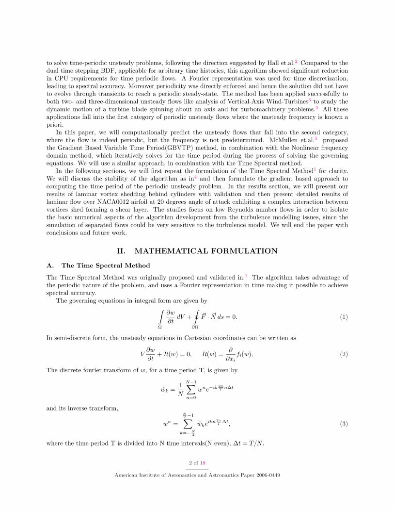
to solve time-periodic unsteady problems, following the direction suggested by Hall et.al.2 Compared to thedual time stepping BDF, applicable for arbitrary time histories, this algorithm showed significant reductionin CPU requirements for time periodic flows. A Fourier representation was used for time discretization,leading to spectral accuracy. Moreover periodicity was directly enforced and hence the solution did not haveto evolve through transients to reach a periodic steady-state. The method has been applied successfully toboth two- and three-dimensional unsteady flows like analysis of Vertical-Axis Wind-Turbines3 to study thedynamic motion of a turbine blade spinning about an axis and for turbomachinery problems.4 All theseapplications fall into the first category of periodic unsteady flows where the unsteady frequency is known apriori.

In this paper, we will computationally predict the unsteady flows that fall into the second category,where the flow is indeed periodic, but the frequency is not predetermined. McMullen et.al.5 proposedthe Gradient Based Variable Time Period(GBVTP) method, in combination with the Nonlinear frequencydomain method, which iteratively solves for the time period during the process of solving the governingequations. We will use a similar approach, in combination with the Time Spectral method.

In the following sections, we will first repeat the formulation of the Time Spectral Method1 for clarity.We will discuss the stability of the algorithm as in4 and then formulate the gradient based approach tocomputing the time period of the periodic unsteady problem. In the results section, we will present ourresults of laminar vortex shedding behind cylinders with validation and then present detailed results oflaminar flow over NACA0012 airfoil at 20 degrees angle of attack exhibiting a complex interaction betweenvortices shed forming a shear layer. The studies focus on low Reynolds number flows in order to isolatethe basic numerical aspects of the algorithm development from the turbulence modelling issues, since thesimulation of separated flows could be very sensitive to the turbulence model. We will end the paper withconclusions and future work.

II. MATHEMATICAL FORMULATION

A. The Time Spectral Method

The Time Spectral Method was originally proposed and validated in.1 The algorithm takes advantage ofthe periodic nature of the problem, and uses a Fourier representation in time making it possible to achievespectral accuracy.

The governing equations in integral form are given by∫

Ω

∂w

∂tdV +

∮

∂Ω

~F · ~N ds = 0. (1)

In semi-discrete form, the unsteady equations in Cartesian coordinates can be written as

V∂w

∂t+ R(w) = 0, R(w) =

∂

∂xifi(w), (2)

The discrete fourier transform of w, for a time period T, is given by

wk =1N

N−1∑n=0

wne−ik 2πT n∆t

and its inverse transform,

wn =

N2 −1∑

k=−N2

wkeikn 2πT ∆t, (3)

where the time period T is divided into N time intervals(N even), ∆t = T/N .

2 of 18


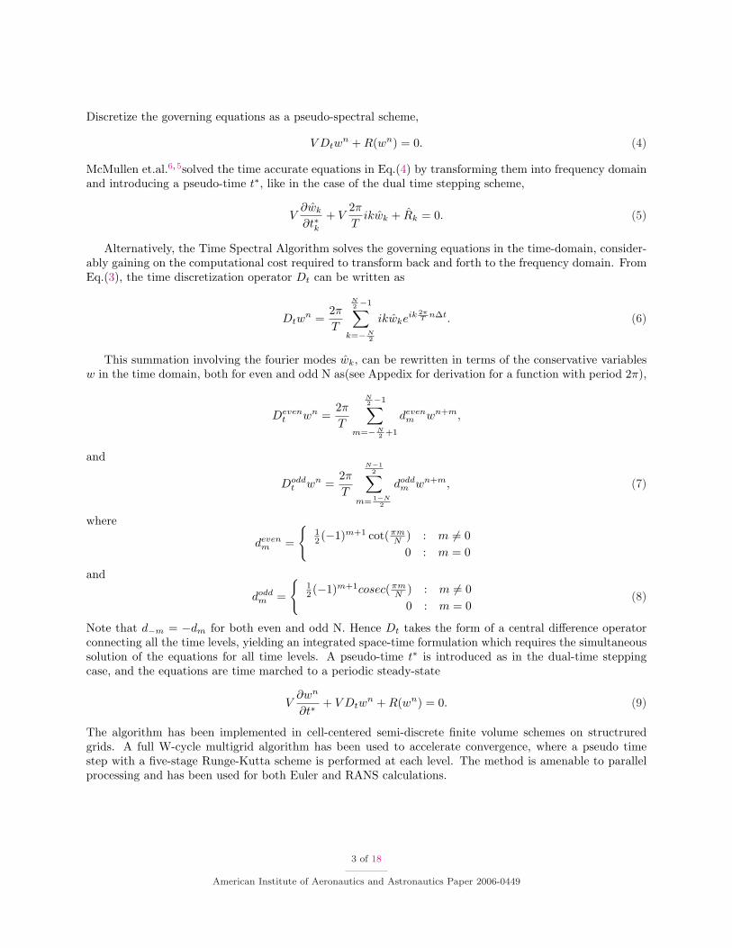
Discretize the governing equations as a pseudo-spectral scheme,

V Dtwn + R(wn) = 0. (4)

McMullen et.al.6,5solved the time accurate equations in Eq.(4) by transforming them into frequency domainand introducing a pseudo-time t∗, like in the case of the dual time stepping scheme,

V∂wk

∂t∗k+ V

2π

Tikwk + Rk = 0. (5)

Alternatively, the Time Spectral Algorithm solves the governing equations in the time-domain, consider-ably gaining on the computational cost required to transform back and forth to the frequency domain. FromEq.(3), the time discretization operator Dt can be written as

Dtwn =

2π

T

N2 −1∑

k=−N2

ikwkeik 2πT n∆t. (6)

This summation involving the fourier modes wk, can be rewritten in terms of the conservative variablesw in the time domain, both for even and odd N as(see Appedix for derivation for a function with period 2π),

Devent wn =

2π

T

N2 −1∑

m=−N2 +1

devenm wn+m,

and

Doddt wn =

2π

T

N−12∑

m= 1−N2

doddm wn+m, (7)

where

devenm =

12 (−1)m+1 cot(πm

N ) : m 6= 00 : m = 0

and

doddm =

12 (−1)m+1cosec(πm

N ) : m 6= 00 : m = 0

(8)

Note that d−m = −dm for both even and odd N. Hence Dt takes the form of a central difference operatorconnecting all the time levels, yielding an integrated space-time formulation which requires the simultaneoussolution of the equations for all time levels. A pseudo-time t∗ is introduced as in the dual-time steppingcase, and the equations are time marched to a periodic steady-state

V∂wn

∂t∗+ V Dtw

n + R(wn) = 0. (9)

The algorithm has been implemented in cell-centered semi-discrete finite volume schemes on structruredgrids. A full W-cycle multigrid algorithm has been used to accelerate convergence, where a pseudo timestep with a five-stage Runge-Kutta scheme is performed at each level. The method is amenable to parallelprocessing and has been used for both Euler and RANS calculations.

3 of 18


B. Stability

The addition of the time derivative term Dtw in equation (9) must be taken into account in the definitionof the pseudo-time step ∆t∗, in comparison with solving a steady-state problem.

Recall Eq. 5

V∂wk

∂t∗k+ V

2π

Tikwk + Rk = 0,

where t∗k is the pseudo-time for wave number k. Note that the orthogonality of the Fourier coefficientsensures that the equations corresponding to each wave number are decoupled. From a stability analysis forthe frequency domain method, the pseudo-time step ∆t∗k can be estimated to be

∆t∗k =CFL ∗ V

||λ||+ k′ ∗ V, (10)

where V is the volume of a cell, ||λ|| is the spectral radius of the flux Jacobian of the spatial part of theequations and k′ = k ∗ 2π

T . I.e. an additional term based on the wave number is added to the denominatorof equation (10) compared to the standard time step definition for a steady-state problem. Hence thepseudo-time step is based on the wave number for each frequency and thus different for every frequency.

To estimate a frequency-based pseudo-time step limit for the Time Spectral Method that is solved in thetime domain, consider the inverse fourier transform of equation (5) back to the time domain,

F−1(V∆wk

∆t∗k+ V

2π

Tikwk + Rk) = 0. (11)

orF−1(V

∆wk

∆t∗k) + V

∂w

∂t+ R(w) = 0. (12)

This inverse fourier transform operation with different time steps ∆t∗k in the frequency domain, will transformto a matrix time step in the time domain coupling all the time levels. As the spectral radius varies fromcell to cell, this matrix will have to be inverted in each cell and at every stage of the multigrid cycle, whichmakes this approach rather costly.

Alternatively, it is possible to use a constant time-step in the frequency domain corresponding to thelargest wave number, i.e. the most restrictive time-step. Then,

∆t∗k =CFL ∗ V

||λ||+ k′ ∗ V(13)

where

k′ =

N2 ∗ 2π

T : N is evenN−1

2 ∗ 2πT : N is odd

(14)

On transforming back to the time domain, the time-step for each time instance is constant and retains theform of ∆t∗k since it is independent of the wave-numbers. The choice of time-step (14) is rather restrictive,especially when the number of time intervals increases. However it considerably reduces the computationalcost involved in inverting a matrix several times.

C. Odd-Even decoupling

Eq. (7) can be written as a matrix vector multiplication

Dtw = DW, (15)

4 of 18


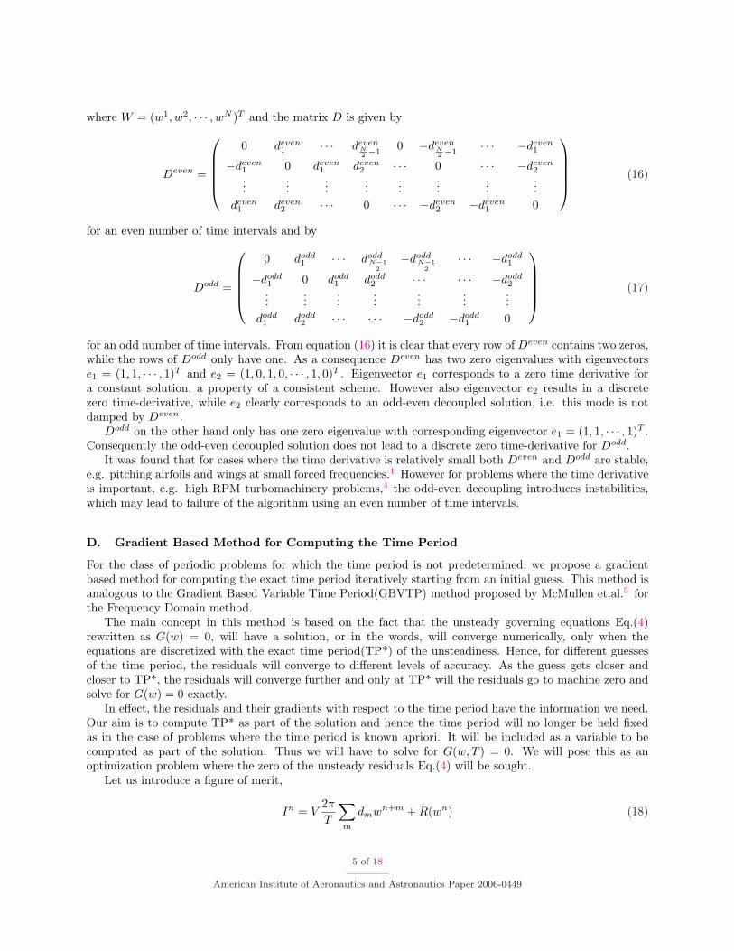
where W = (w1, w2, · · · , wN )T and the matrix D is given by

Deven =

0 deven1 · · · deven

N2 −1

0 −devenN2 −1

· · · −deven1

−deven1 0 deven

1 deven2 · · · 0 · · · −deven

2...

......

......

......

...deven1 deven

2 · · · 0 · · · −deven2 −deven

1 0

(16)

for an even number of time intervals and by

Dodd =

0 dodd1 · · · dodd

N−12

−doddN−1

2· · · −dodd

1

−dodd1 0 dodd

1 dodd2 · · · · · · −dodd

2...

......

......

......

dodd1 dodd

2 · · · · · · −dodd2 −dodd

1 0

(17)

for an odd number of time intervals. From equation (16) it is clear that every row of Deven contains two zeros,while the rows of Dodd only have one. As a consequence Deven has two zero eigenvalues with eigenvectorse1 = (1, 1, · · · , 1)T and e2 = (1, 0, 1, 0, · · · , 1, 0)T . Eigenvector e1 corresponds to a zero time derivative fora constant solution, a property of a consistent scheme. However also eigenvector e2 results in a discretezero time-derivative, while e2 clearly corresponds to an odd-even decoupled solution, i.e. this mode is notdamped by Deven.

Dodd on the other hand only has one zero eigenvalue with corresponding eigenvector e1 = (1, 1, · · · , 1)T .Consequently the odd-even decoupled solution does not lead to a discrete zero time-derivative for Dodd.

It was found that for cases where the time derivative is relatively small both Deven and Dodd are stable,e.g. pitching airfoils and wings at small forced frequencies.1 However for problems where the time derivativeis important, e.g. high RPM turbomachinery problems,4 the odd-even decoupling introduces instabilities,which may lead to failure of the algorithm using an even number of time intervals.

D. Gradient Based Method for Computing the Time Period

For the class of periodic problems for which the time period is not predetermined, we propose a gradientbased method for computing the exact time period iteratively starting from an initial guess. This method isanalogous to the Gradient Based Variable Time Period(GBVTP) method proposed by McMullen et.al.5 forthe Frequency Domain method.

The main concept in this method is based on the fact that the unsteady governing equations Eq.(4)rewritten as G(w) = 0, will have a solution, or in the words, will converge numerically, only when theequations are discretized with the exact time period(TP*) of the unsteadiness. Hence, for different guessesof the time period, the residuals will converge to different levels of accuracy. As the guess gets closer andcloser to TP*, the residuals will converge further and only at TP* will the residuals go to machine zero andsolve for G(w) = 0 exactly.

In effect, the residuals and their gradients with respect to the time period have the information we need.Our aim is to compute TP* as part of the solution and hence the time period will no longer be held fixedas in the case of problems where the time period is known apriori. It will be included as a variable to becomputed as part of the solution. Thus we will have to solve for G(w, T ) = 0. We will pose this as anoptimization problem where the zero of the unsteady residuals Eq.(4) will be sought.

Let us introduce a figure of merit,

In = V2π

T

∑m

dmwn+m + R(wn) (18)

5 of 18


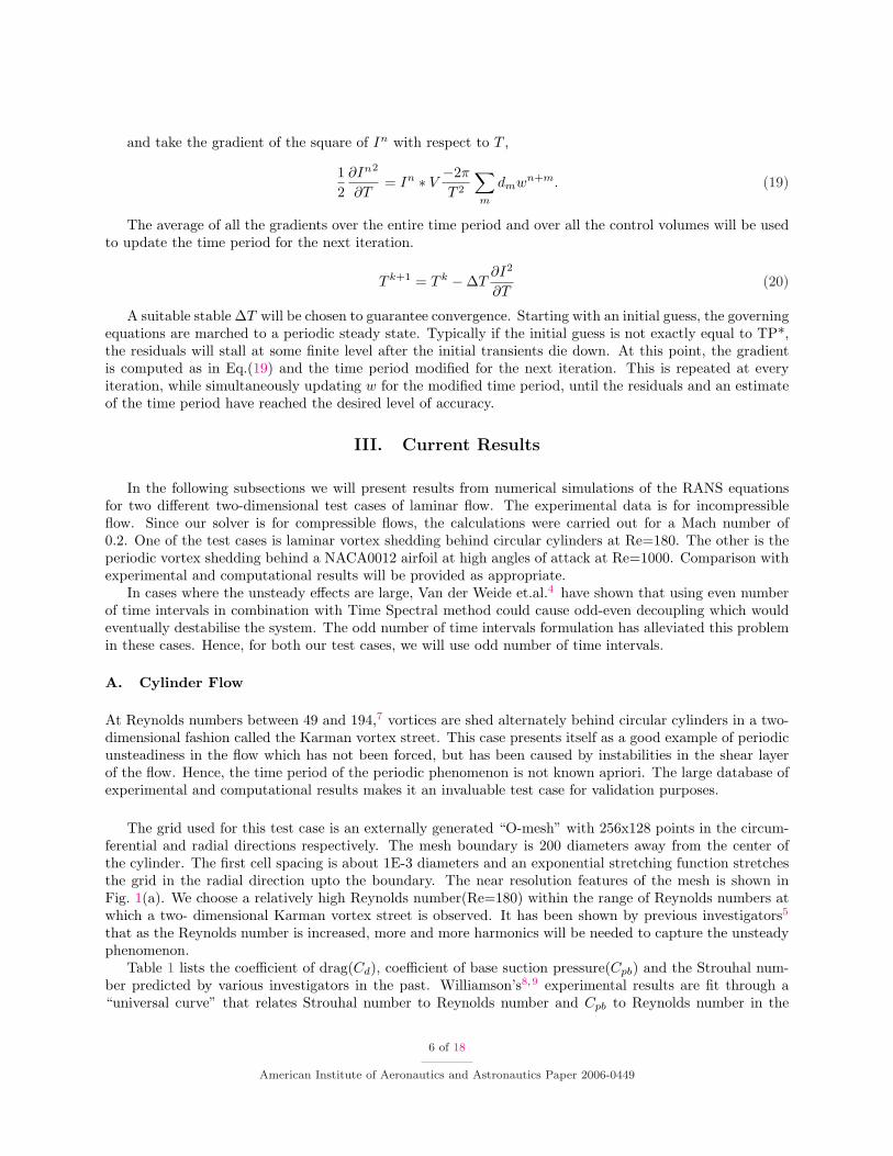
and take the gradient of the square of In with respect to T ,

12

∂In2

∂T= In ∗ V

−2π

T 2

∑m

dmwn+m. (19)

The average of all the gradients over the entire time period and over all the control volumes will be usedto update the time period for the next iteration.

T k+1 = T k −∆T∂I2

∂T(20)

A suitable stable ∆T will be chosen to guarantee convergence. Starting with an initial guess, the governingequations are marched to a periodic steady state. Typically if the initial guess is not exactly equal to TP*,the residuals will stall at some finite level after the initial transients die down. At this point, the gradientis computed as in Eq.(19) and the time period modified for the next iteration. This is repeated at everyiteration, while simultaneously updating w for the modified time period, until the residuals and an estimateof the time period have reached the desired level of accuracy.

III. Current Results

In the following subsections we will present results from numerical simulations of the RANS equationsfor two different two-dimensional test cases of laminar flow. The experimental data is for incompressibleflow. Since our solver is for compressible flows, the calculations were carried out for a Mach number of0.2. One of the test cases is laminar vortex shedding behind circular cylinders at Re=180. The other is theperiodic vortex shedding behind a NACA0012 airfoil at high angles of attack at Re=1000. Comparison withexperimental and computational results will be provided as appropriate.

In cases where the unsteady effects are large, Van der Weide et.al.4 have shown that using even numberof time intervals in combination with Time Spectral method could cause odd-even decoupling which wouldeventually destabilise the system. The odd number of time intervals formulation has alleviated this problemin these cases. Hence, for both our test cases, we will use odd number of time intervals.

A. Cylinder Flow

At Reynolds numbers between 49 and 194,7 vortices are shed alternately behind circular cylinders in a two-dimensional fashion called the Karman vortex street. This case presents itself as a good example of periodicunsteadiness in the flow which has not been forced, but has been caused by instabilities in the shear layerof the flow. Hence, the time period of the periodic phenomenon is not known apriori. The large database ofexperimental and computational results makes it an invaluable test case for validation purposes.

The grid used for this test case is an externally generated “O-mesh” with 256x128 points in the circum-ferential and radial directions respectively. The mesh boundary is 200 diameters away from the center ofthe cylinder. The first cell spacing is about 1E-3 diameters and an exponential stretching function stretchesthe grid in the radial direction upto the boundary. The near resolution features of the mesh is shown inFig. 1(a). We choose a relatively high Reynolds number(Re=180) within the range of Reynolds numbers atwhich a two- dimensional Karman vortex street is observed. It has been shown by previous investigators5

that as the Reynolds number is increased, more and more harmonics will be needed to capture the unsteadyphenomenon.

Table 1 lists the coefficient of drag(Cd), coefficient of base suction pressure(Cpb) and the Strouhal num-ber predicted by various investigators in the past. Williamson’s8,9 experimental results are fit through a“universal curve” that relates Strouhal number to Reynolds number and Cpb to Reynolds number in the

6 of 18


(a) Cylinder Flow - O mesh (b) High Alpha Airfoil - C mesh

Figure 1.

Experiment −Cpb Cd St

Williamson8,9 0.9198 0.1919Roshko10 0.185

Henderson11 0.9599 1.336

Table 1. Time-Averaged coefficients and Strouhal number from previous investigators

#Time Intervals −Cpb Cd St

5 .9203 1.3324 .18847 .9258 1.3339 .18659 .9332 1.3392 .186611 .9348 1.3404 .186713 .9351 1.3406 .186621 .9351 1.3406 .1866

Table 2. Time-Averaged coefficients and Strouhal number computed with various #Time Intervals

7 of 18


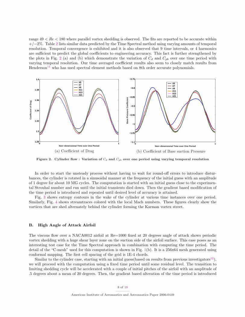
range 49 < Re < 180 where parallel vortex shedding is observed. The fits are reported to be accurate within+/−2%. Table 2 lists similar data predicted by the Time Spectral method using varying amounts of temporalresolution. Temporal convergence is exhibited and it is also observed that 9 time intervals, or 4 harmonicsare sufficient to predict the global coefficients to engineering accuracy. This fact is further strengthened bythe plots in Fig. 2 (a) and (b) which demonstrate the variation of Cd and Cpb over one time period withvarying temporal resolution. Our time averaged coefficient results also seem to closely match results fromHenderson11 who has used spectral element methods based on 8th order accurate polynomials.

0 11.28

1.3

1.32

1.34

1.36

1.38

1.4

Non−dimensional Time over One Period

Coe

ffici

ent o

f Dra

g

it5it7it9it11it13it21

(a) Coefficient of Drag

0 1−1.1

−1.05

−1

−0.95

−0.9

−0.85

−0.8

−0.75


Bas

e P

ress

ure

Coe

ffici

ent


(b) Coefficient of Base suction Pressure

Figure 2. Cylinder flow : Variation of Cd and Cpb over one period using varying temporal resolution

In order to start the unsteady process without having to wait for round-off errors to introduce distur-bances, the cylinder is rotated in a sinusoidal manner at the frequency of the initial guess with an amplitudeof 1 degree for about 10 MG cycles. The computation is started with an initial guess close to the experimen-tal Strouhal number and run until the initial transients died down. Then the gradient based modification ofthe time period is introduced and repeated until desired level of accuracy is attained.

Fig. 3 shows entropy contours in the wake of the cylinder at various time instances over one period.Similarly, Fig. 4 shows streamtraces colored with the local Mach numbers. These figures clearly show thevortices that are shed alternately behind the cylinder forming the Karman vortex street.

B. High Angle of Attack Airfoil

The viscous flow over a NACA0012 airfoil at Re=1000 fixed at 20 degrees angle of attack shows periodicvortex shedding with a huge shear layer zone on the suction side of the airfoil surface. This case poses as aninteresting test case for the Time Spectral approach in combination with computing the time period. Thedetail of the “C-mesh” used for this computation is shown in Fig. 1(b). It is a 256x64 mesh generated usingconformal mapping. The first cell spacing of the grid is 1E-4 chords.

Similar to the cylinder case, starting with an initial guess(based on results from previous investigators12),we will proceed with the computation using a fixed time period until some residual level. The transition tolimiting shedding cycle will be accelerated with a couple of initial pitches of the airfoil with an amplitude of.5 degrees about a mean of 20 degrees. Then, the gradient based alteration of the time period is introduced

8 of 18


(a) t = 0 (b) t = T3 (c) t = 2T

3

Figure 3. Cylinder flow : Entropy contours at various time instances over one period

(a) t = 0 (b) t = T3 (c) t = 2T

3

Figure 4. Cylinder flow : Streamtraces colored by Mach number at various time instances over one period

9 of 18


to achieve a desired level of accuracy both for the unsteady solution and the estimate of the exact timeperiod(TP*).

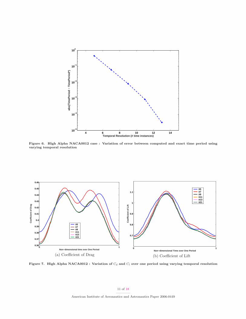
Fig. 5 shows convergence to the exact time period starting from the initial guess using various levels oftemporal resolution. Note that as the number of time intervals is increased, the converged time period getscloser to TP*,i.e. temporal convergence is achieved. Atleast 9 time intervals are required to predict TP*to engineering accuracy. Fig. 6 shows the error in the computed time period using varying number of timeintervals per period, based on TP* computed with N = 21. It proves that close to exponential convergencehas been achieved which is evidenced from the linear variation of the error on a semi-log plot.

0 200 400 600 800 1000 12008.1

8.2

8.3

8.4

8.5

8.6

8.7

8.8

8.9

9

# Multigrid Cycles

Tim

e P

erio

d

it5

it7

it9

it11

it13

Figure 5. High Alpha NACA0012 case : Convergence from initial guess to exact Time Period with varyingtemporal resolution

The observation that N = 9 is all that is required to achieve engineering accuracy is further affirmedby the plots showing variation of Coefficient of Drag(Fig. 7(a)) and Coefficient of Lift(Fig. 7(b)) over oneperiod computed using varying N .

Another set of results were assimilated based on different starting guesses for the time period. All of themwere simulated with N = 9 and Fig. 8 shows their convergence to the same time period using the gradientbased approach. The percentages listed are the differences in percentage between the exact time periodand the initial guess. This trend eliminates any random results that can occur with a single initial guesscomputation.

Fig. 9 shows convergence trends of the solution of unsteady residuals while holding the time period fixedand using 11 time intervals. With an approximate time period 2.75% different from TP*, the solutionconverges 3 orders of magnitude and stalls. With a time period computed using the gradient based approachand accurate upto 6 orders of magnitude, the residuals converge further and saturate at 6 orders of magnitude.Also shown is a computation with time period 7.5% different from TP* which saturates at a higher level ofaccuracy. This confirms that the accuracy of the time period of periodic unsteadiness directly dictates thelevel of accuracy of the unsteady residuals of the discrete system of equations.

Fig. 10 shows entropy contours at various time instances over one period. Similarly, Fig. 11 showsstreamtraces colored with the local Mach numbers. These figures clearly show the vortices shed periodically

10 of 18


4 6 8 10 12 1410

−5

10−4

10−3

10−2

10−1

100

Temporal Resolution (# time instances)

abs(

Tim

ePer

iod

− T

imeP

erio

d*)

Figure 6. High Alpha NACA0012 case : Variation of error between computed and exact time period usingvarying temporal resolution

0 10.36

0.37

0.38

0.39

0.4

0.41

0.42

0.43

0.44

0.45

0.46

Non−dimensional time over One Period

Coe

ffici

ent o

f Dra

g


(a) Coefficient of Drag

0 1

0.7

0.8

0.9

1

1.1


Coe

ffici

ent o

f Lift


(b) Coefficient of Lift

Figure 7. High Alpha NACA0012 : Variation of Cd and Cl over one period using varying temporal resolution

11 of 18


0 200 400 600 800 1000 12007.6

7.8

8

8.2

8.4

8.6

8.8

9

# Multigrid Cycles

Tim

e P

erio

d

+ 2.75%− 2.75%+ 5 %− 5 %+7.5 %

Figure 8. High Alpha NACA0012 Case : Various time period starting guesses converging to same exact timeperiod

0 1000 2000 3000 4000 500010

−6

10−5

10−4

10−3

10−2

10−1

100

101

# Multigrid Cycles

RM

S D

ensi

ty R

esid

ual

approx TP : 7.5% errorexact TPapprox TP : 2.5% error

Figure 9. High Alpha NACA0012 Case : Convergence of RMS Density Residual with approx and exact timeperiod

12 of 18


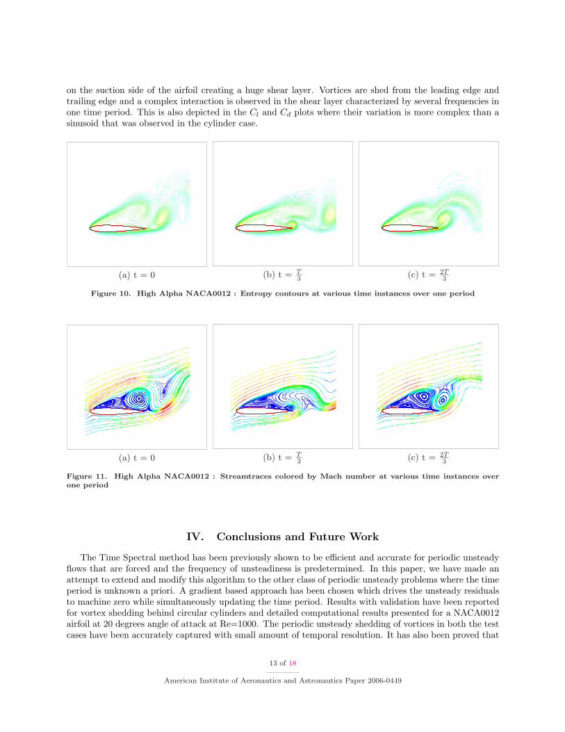
on the suction side of the airfoil creating a huge shear layer. Vortices are shed from the leading edge andtrailing edge and a complex interaction is observed in the shear layer characterized by several frequencies inone time period. This is also depicted in the Cl and Cd plots where their variation is more complex than asinusoid that was observed in the cylinder case.

(a) t = 0 (b) t = T3 (c) t = 2T

3

Figure 10. High Alpha NACA0012 : Entropy contours at various time instances over one period

(a) t = 0 (b) t = T3 (c) t = 2T

3

Figure 11. High Alpha NACA0012 : Streamtraces colored by Mach number at various time instances overone period

IV. Conclusions and Future Work

The Time Spectral method has been previously shown to be efficient and accurate for periodic unsteadyflows that are forced and the frequency of unsteadiness is predetermined. In this paper, we have made anattempt to extend and modify this algorithm to the other class of periodic unsteady problems where the timeperiod is unknown a priori. A gradient based approach has been chosen which drives the unsteady residualsto machine zero while simultaneously updating the time period. Results with validation have been reportedfor vortex shedding behind circular cylinders and detailed computational results presented for a NACA0012airfoil at 20 degrees angle of attack at Re=1000. The periodic unsteady shedding of vortices in both the testcases have been accurately captured with small amount of temporal resolution. It has also been proved that

13 of 18


to get an accurate solution of the discretized equations, it is important to predict the time period to a similarlevel of accuracy. A small percentage of error could lead to a completely different solution. It is also necessaryto use at least the minimum amount of temporal resolution needed to capture the unsteady phenomenon inorder to predict the right time period. These two features will assure a machine-level accurate solution ofthe governing equations.

In the future, we would like to make this approach more robust by trying various other optimizationstrategies, better ways of providing an initial guess or providing not-so-close initial guesses and still obtainconvergence, faster convergence, adaptively increasing the temporal resolution as needed etc. Artificialcompressibility could be introduced in combination with a compressible solver to improve efficiency andaccuracy. Adaptive mesh refinement could be introduced in order to capture the vortices better.

This is a first step towards predicting unsteady flows about high-lift single/multi-element airfoils/wings.Transonic test cases and realistic test conditions would be an ideal extension. Further, we would like tosimulate the effect of unsteady blowing/suction by synthetic jets to reduce separation effects. The TimeSpectral method with the capability of simulating both forced periodic unsteadiness and that caused byinstabilities, would be a fit candidate for problems with complex interactions between forced and instabilityinduced unsteadiness.

V. ACKNOWLEDGMENT

This work has benefited from the generous support of the Department of Energy under contract numberLLNL B341491 as part of the Advanced Scientific Computing(ASC) program at Stanford University.

References

1A. Gopinath and A. Jameson. Time spectral method for periodic unsteady computations over two- and three-dimensionalbodies. AIAA paper 05-1220, AIAA 43rd Aerospace Sciences Meeting and Exhibit, Reno, NV, January 10-13 2005.

2K.C. Hall, J.P. Thomas, and W.S. Clark. Computation of unsteady nonlinear flows in cascades using a harmonic balancetechnique. AIAA Journal, 40(5):879–886, May 2002.

3J.C.Vassberg, A.Gopinath, and A.Jameson. Revisiting the vertical-axis wind-turbine design using advanced computationalfluid dynamics. AIAA paper 05-0047, 43rd AIAA Aerospace Sciences Meeting and Exhibit, Reno, NV, January 10-13 2005.

4E. Van der Weide, A. Gopinath, and A. Jameson. Turbomachinery applications with the time spectral method. AIAApaper 05-4905, 17th AIAA Computational Fluid Dynamics Conference, Toronto, Ontario, June 6-9 2005.

5M. McMullen, A. Jameson, and J.J. Alonso. Application of a non-linear frequency domain solver to the euler andnavier-stokes equations. AIAA paper 02-0120, AIAA 40th Aerospace Sciences Meeting and Exhibit, Reno, NV, January 2002.

6M. McMullen, A. Jameson, and J.J. Alonso. Acceleration of convergence to a periodic steady state in turbomachineryflows. AIAA paper 01-0152, AIAA 39th Aerospace Sciences Meeting, Reno, NV, January 2001.

7C.H.K.Williamson. Vortex dynamics in the cylinder wake. Technical Report 28:477-539, Annual Review Fluid Mech.,1996.

8C.H.K.Williamson. Defining a universal and contiguous strouhal-reynolds number relationship of the laminar vortexshedding of a circular cylinder. Technical Report 31:2747-2747, Physics of Fluids, October 1988.

9C.H.K.Williamson. Measurements of base pressure in the wake of a cylinder at low reynolds numbers. Technical Re-port 14:pp.38-46, Z.Flugwiss, Weltraumforsch,, 1990.

10A.Roshko. On the development of turbulent wakes from vortex streets. Technical report, NACA Technical Report 1191,NACA, January 1954.

11R.D.Henderson. Details of the drag curve near the onset of vortex shedding. Technical report, Physics of Fluids, 1995.12A.A.Belov. A new implicit multigrid-driven algorithm for unsteady incompressible flow calculations on parallel computers.

Technical report, Dissertation, Princeton University, June 1997.13P.Moin. Me308 spectral methods in computational physics. Technical report, Class notes provided as part of Stanford’s

ME308 Course, 1997.14A.Quarteroni C.Canuto, M.Y.Hussaini and T.A. Zang. Spectral Methods in Fluid Dynamics; Springer Series in Compu-

tational Physics. Springer Verlag, 1988.

14 of 18


A. APPENDIX

A. Matrix Operators for Numerical Differentiation

In this section we shall present a physical operator for numerical differentiation13 of a periodic discretefunction discussed over two parts. One for even number of discretization points and the other for odd. Theresults for even formulation can be found in14 and is used extensively for computations using FFTs.

Let u be a function defined on the grid between 0 ≤ x ≤ 2π,

xj =2πj

Nj = 0, 1, 2, ...N − 1.

1. Even Formulation

Discrete Fourier transform of u is given by

uk =1N

N−1∑

j=0

u(xj)e−ikxj


u(xj) =

N2 −1∑

k=−N2

ukeikxj

The spectral derivative of u at the grid points is given by

(Du)j =

N2 −1∑

k=−N2 +1

ikukeikxj ,

where we have set the Fourier coefficient corresponding to the oddball wave number equal to zero. Substi-tuting for uk from the Fourier transform, we obtain

(Du)l =1N

N2 −1∑

k=−N2 +1

N−1∑

j=0

iku(xj)e−ikxj eikxl .

or(Du)l =

1N

∑

k

∑

j

ikuje2πik

N (l−j).

Let

dlj =1N

N2 −1∑

k=−N2 +1

ike2πik

N (l−j) (21)

Then

(Du)l =N−1∑

j=0

dljuj

which expresses multiplication of a matrix with elements dlj and the vector u. It turns out that dlj can becomputed analytically. To evaluate the sum in (21), recall that from geometric series, we have

S =

N2 −1∑

k=−N2 +1

eikx = ei(−N2 +1)x + ei(−N

2 +2)x + ... + ei( N2 −1)x

15 of 18


or

S = ei(−N2 +1)x[1 + eix + e2ix + ...ei(N−2)x] = ei(−N

2 +1)x 1− ei(N−1)x

1− eix

or

S =ei(−N

2 +1)x − ei( N2 )x

1− eix=

ei(−N2 + 1

2 )x − ei( N2 − 1

2 )x

e−i x2 − ei x

2=

sin(N−12 x)

sin x2

This expression can be differentiated to yield the desired sum

dS

dx=

N2 −1∑

k=−N2 +1

ikeikx =(N−1

2 ) cos(N−12 x) sin x

2 − 12 cos x

2 sin(N−12 x)

(sin x2 )2

This expression can be simplified using trigonometric identities and noting that x = 2πN (l − j),

sin(Nx

2− x

2) = −(−1)l−j sin

x

2

cos(Nx

2− x

2) = (−1)l−j cos

x

2Therefore,

dS

dx=

(N−12 )(−1)l−j cos x

2 sin x2 + 1

2 (−1)l−j cos x2 sin x

2

(sin x2 )2

ordS

dx=

N2 (−1)l−j cos x

2 sin x2

(sin x2 )2

=N

2(−1)l−j cot

x

2

Thus,

dlj =

12 (−1)l−j cot(π(l−j)

N ) : l 6= j

0 : l = j

With a change of variables, -m = (l-j), we have,

dm =

12 (−1)m+1 cot(πm

N ) : m 6= 00 : m = 0

This change of variables shows that D is indeed a central difference operator since d−m = −dm

2. Odd Formulation

Discrete Fourier transform of u is given by

uk =1N

N−1∑

j=0

u(xj)e−ikxj


u(xj) =

N−12∑

k=−N−12

ukeikxj

16 of 18


The spectral derivative of u at the grid points is given by

(Du)j =

N−12∑

k=−N−12

ikukeikxj .

Note that for odd N there is no oddball element. Substituting for uk from the Fourier transform, we obtain

(Du)l =1N

N−12∑

k=−N−12

N−1∑

j=0

iku(xj)e−ikxj eikxl .

or(Du)l =

1N

∑

k

∑

j

ikuje2πik

N (l−j).

Let

dlj =1N

N−12∑

k=−N−12

ike2πik

N (l−j) (22)

Then

(Du)l =N−1∑

j=0

dljuj .

To evaluate the sum in ( 22), we have

S =

N−12∑

k=−N−12

eikx = ei(−N−12 )x + ei(−N−1

2 +1)x + ... + ei( N−12 )x

or

S = ei(−N−12 )x[1 + eix + e2ix + ...ei(N−1)x] = ei(−N−1

2 )x 1− eiNx

1− eix

or

S =ei(−N−1

2 )x − ei( N+12 )x

1− eix=

ei(−N2 )x − ei( N

2 )x

e−i x2 − ei x

2=

sin(N2 x)

sin x2

This expression will be differentiated to yield the desired sum

dS

dx=

N−12∑

k=−N−12

ikeikx =(N

2 ) cos(N2 x) sin x

2 − 12 cos x

2 sin(N2 x)

(sin x2 )2

This expression can be simplified using trigonometric identities and noting that x = 2πN (l − j),

sin(Nx

2) = 0

cos(Nx

2) = (−1)l−j

Therefore,dS

dx=

(N2 )(−1)l−j sin x

2

(sin x2 )2

17 of 18


ordS

dx=

N

2(−1)l−jcosec

x

2Thus,

dlj =

12 (−1)l−jcosec(π(l−j)

N ) : l 6= j

0 : l = j

With a change of variables, -m = (l-j), we have,

dm =

12 (−1)m+1cosec(πm

N ) : m 6= 00 : m = 0

The central difference operator form still holds for odd N.

18 of 18


Documents

44th AIAA Aerospace Sciences Meeting and Exhibit, …aero-comlab.stanford.edu/arathi/TSComputeTimep.pdfArathi K. Gopinath⁄, and Antony Jameson y ... the periodic nature of the problem,