Embed Size (px)
Citation preview
International Prices and Exchange RatesGita Gopinath
• Nominal and Real Exchange Rates
• Exchange-rate pass-through and expenditure switching
• Currency Wars, Fear of Floating
1 / 72
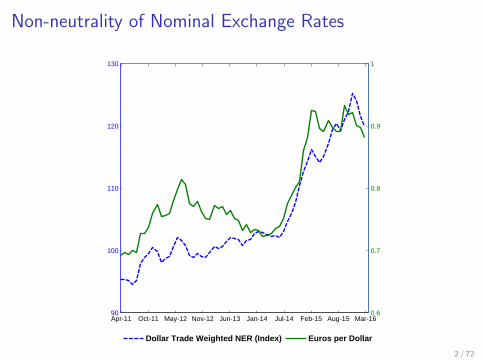
Non-neutrality of Nominal Exchange Rates
Apr-11 Oct-11 May-12 Nov-12 Jun-13 Jan-14 Jul-14 Feb-15 Aug-15 Mar-1690
100
110
120
130
0.6
0.7
0.8
0.9
1
Dollar Trade Weighted NER (Index) Euros per Dollar
2 / 72

International SpilloversNominal Rigidities
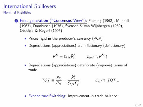
1 First generation (“Consensus View”): Fleming (1962), Mundell
(1963), Dornbusch (1976), Svenson & van Wijnbergen (1989),Obstfeld & Rogoff (1995)
• Prices rigid in the producer’s currency (PCP)
• Depreciations (appreciations) are inflationary (deflationary)
PM = Eh/f Pff Eh/f ↑,PM ↑
• Depreciations (appreciations) deteriorate (improve) terms oftrade.
TOT ≡ PX
PM=
Phh
Eh/f Pff
Eh/f ↑,TOT ↓
• Expenditure Switching: Improvement in trade balance.
3 / 72
International SpilloversNominal Rigidities
1 First generation (“Consensus View”): Fleming (1962), Mundell
(1963), Dornbusch (1976), Svenson & van Wijnbergen (1989),Obstfeld & Rogoff (1995)
• Prices rigid in the producer’s currency (PCP)
• Depreciations (appreciations) are inflationary (deflationary)
PM = Eh/f Pff Eh/f ↑,PM ↑
• Depreciations (appreciations) deteriorate (improve) terms oftrade.
TOT ≡ PX
PM=
Phh
Eh/f Pff
Eh/f ↑,TOT ↓
• Expenditure Switching: Improvement in trade balance.
3 / 72

International SpilloversNominal Rigidities
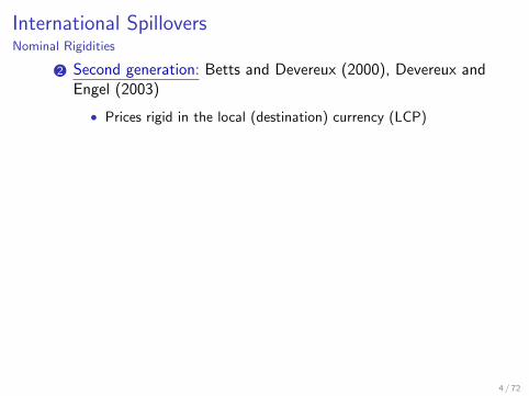
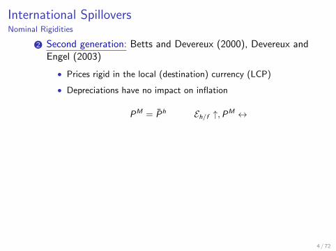
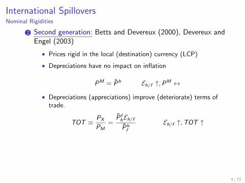
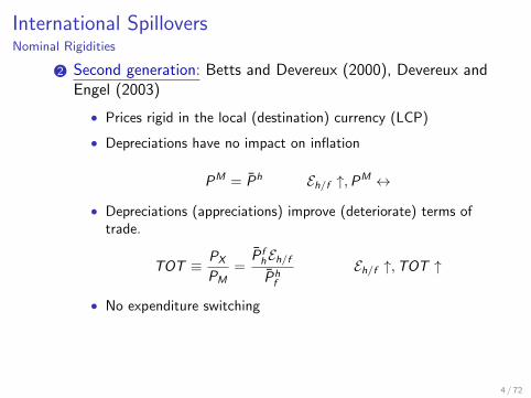
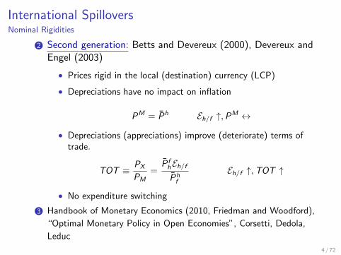
2 Second generation: Betts and Devereux (2000), Devereux andEngel (2003)
• Prices rigid in the local (destination) currency (LCP)
• Depreciations have no impact on inflation
PM = Ph Eh/f ↑,PM ↔
• Depreciations (appreciations) improve (deteriorate) terms oftrade.
TOT ≡ PX
PM=
P fhEh/f
Phf
Eh/f ↑,TOT ↑
• No expenditure switching
3 Handbook of Monetary Economics (2010, Friedman and Woodford),
“Optimal Monetary Policy in Open Economies”, Corsetti, Dedola,
Leduc
4 / 72
International SpilloversNominal Rigidities
2 Second generation: Betts and Devereux (2000), Devereux andEngel (2003)
• Prices rigid in the local (destination) currency (LCP)
• Depreciations have no impact on inflation
PM = Ph Eh/f ↑,PM ↔
• Depreciations (appreciations) improve (deteriorate) terms oftrade.
TOT ≡ PX
PM=
P fhEh/f
Phf
Eh/f ↑,TOT ↑
• No expenditure switching
3 Handbook of Monetary Economics (2010, Friedman and Woodford),
“Optimal Monetary Policy in Open Economies”, Corsetti, Dedola,
Leduc
4 / 72

What does micro data tells us?
1 Neither PCP, nor LCP, but pricing in very few currencies• Outsized role for dollar
2 Prices are rigid in their currency of invoicing
3 Conditional on a price change prices not very sensitive toexchange rates
• Strategic complementarity in pricing• Variable desired mark-ups
• Imported intermediate inputs
4 Dominant Currency Paradigm: 1+2+3
5 / 72

Road Map
• Dominant currencies
• Model
• Empirical Evidence
6 / 72
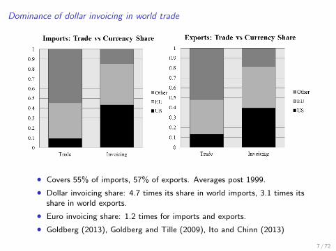
Dominance of dollar invoicing in world trade
• Covers 55% of imports, 57% of exports. Averages post 1999.
• Dollar invoicing share: 4.7 times its share in world imports, 3.1 times itsshare in world exports.
• Euro invoicing share: 1.2 times for imports and exports.
• Goldberg (2013), Goldberg and Tille (2009), Ito and Chinn (2013)
7 / 72
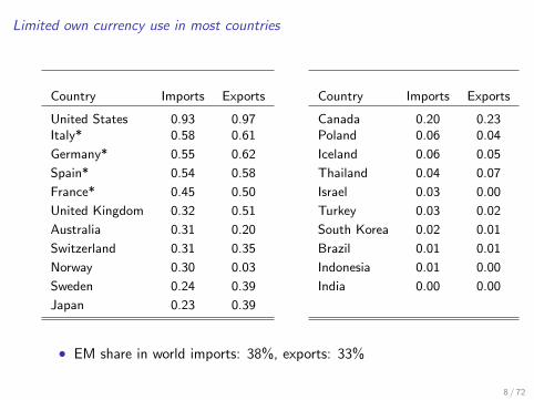
Limited own currency use in most countries
Country Imports Exports Country Imports Exports
United States 0.93 0.97 Canada 0.20 0.23Italy* 0.58 0.61 Poland 0.06 0.04
Germany* 0.55 0.62 Iceland 0.06 0.05
Spain* 0.54 0.58 Thailand 0.04 0.07
France* 0.45 0.50 Israel 0.03 0.00
United Kingdom 0.32 0.51 Turkey 0.03 0.02
Australia 0.31 0.20 South Korea 0.02 0.01
Switzerland 0.31 0.35 Brazil 0.01 0.01
Norway 0.30 0.03 Indonesia 0.01 0.00
Sweden 0.24 0.39 India 0.00 0.00
Japan 0.23 0.39
• EM share in world imports: 38%, exports: 33%
8 / 72
Model: New Keynesian small open economy
• Building Blocks• Sticky Prices and or Sticky Wages (Calvo)• Household and Firms• Asset markets• Monetary policy
• Home H trades with U (dominant currency) and R
• All prices and quantities in U and R are exogenous (constant)
9 / 72
Model: New Keynesian small open economy
• Building Blocks• Sticky Prices and or Sticky Wages (Calvo)• Household and Firms• Asset markets• Monetary policy
• Home H trades with U (dominant currency) and R
• All prices and quantities in U and R are exogenous (constant)
9 / 72
Households
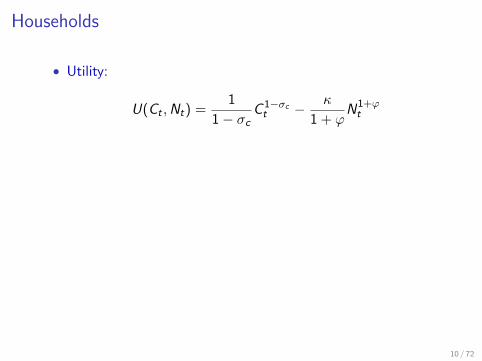
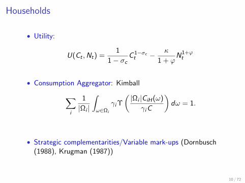
• Utility:
U(Ct ,Nt) =1
1− σcC 1−σc
t − κ
1 + ϕN1+ϕ
t
• Consumption Aggregator: Kimball∑i
1
|Ωi |
∫ω∈Ωi
γi Υ
(|Ωi |CiH(ω)
γiC
)dω = 1.
• Strategic complementarities/Variable mark-ups (Dornbusch(1988), Krugman (1987))
10 / 72
Households
• Utility:
U(Ct ,Nt) =1
1− σcC 1−σc
t − κ
1 + ϕN1+ϕ
t
• Consumption Aggregator: Kimball∑i
1
|Ωi |
∫ω∈Ωi
γi Υ
(|Ωi |CiH(ω)
γiC
)dω = 1.
• Strategic complementarities/Variable mark-ups (Dornbusch(1988), Krugman (1987))
10 / 72
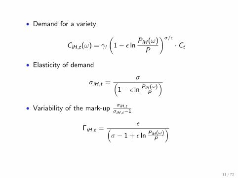
• Demand for a variety
CiH,t(ω) = γi
(1− ε ln
PiH(ω)
P
)σ/ε· Ct
• Elasticity of demand
σiH,t =σ(
1− ε ln PiH (ω)P
)• Variability of the mark-up
σiH,t
σiH,t−1
ΓiH,t =ε(
σ − 1 + ε ln PiH (ω)P
)
11 / 72
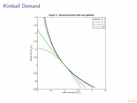
Kimball Demand
0 0.5 1 1.5 2 2.50.85
0.9
0.95
1
1.05
1.1
1.15
1.2
1.25
1.3Figure 1: Demand function with real rigidities
rela
tive
pric
e (P
si/P
s)
relative demand (Ysi
/Ys)
ε = 0ε = 1ε = 5ε = 10
17
12 / 72
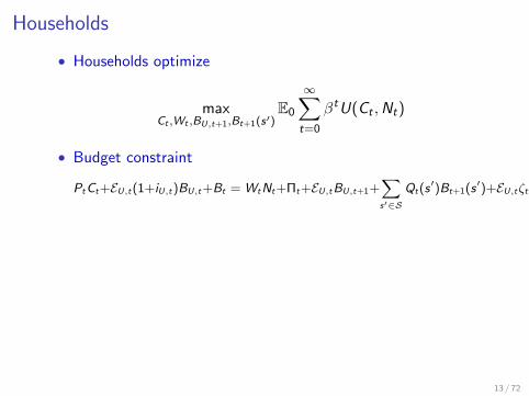
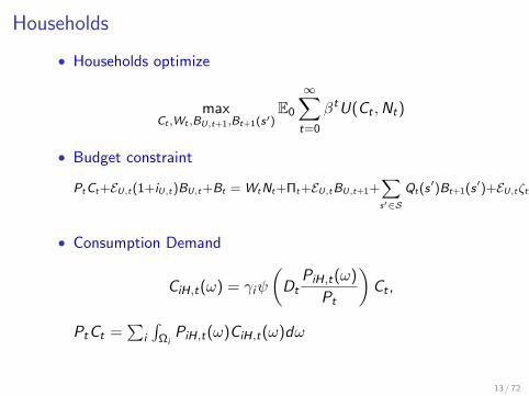
Households
• Households optimize
maxCt ,Wt ,BU,t+1,Bt+1(s′)
E0
∞∑t=0
βtU(Ct ,Nt)
• Budget constraint
PtCt+EU,t(1+iU,t)BU,t+Bt = WtNt+Πt+EU,tBU,t+1+∑s′∈S
Qt(s ′)Bt+1(s ′)+EU,tζt
• Consumption Demand
CiH,t(ω) = γiψ
(Dt
PiH,t(ω)
Pt
)Ct ,
PtCt =∑
i
∫Ωi
PiH,t(ω)CiH,t(ω)dω
13 / 72
Households
• Households optimize
maxCt ,Wt ,BU,t+1,Bt+1(s′)
E0
∞∑t=0
βtU(Ct ,Nt)
• Budget constraint
PtCt+EU,t(1+iU,t)BU,t+Bt = WtNt+Πt+EU,tBU,t+1+∑s′∈S
Qt(s ′)Bt+1(s ′)+EU,tζt
• Consumption Demand
CiH,t(ω) = γiψ
(Dt
PiH,t(ω)
Pt
)Ct ,
PtCt =∑
i
∫Ωi
PiH,t(ω)CiH,t(ω)dω
13 / 72
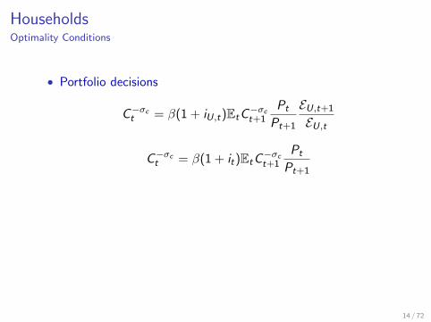
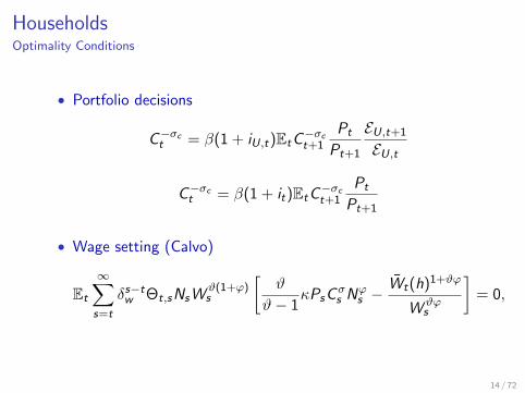
HouseholdsOptimality Conditions
• Portfolio decisions
C−σct = β(1 + iU,t)EtC
−σct+1
Pt
Pt+1
EU,t+1
EU,t
C−σct = β(1 + it)EtC
−σct+1
Pt
Pt+1
• Wage setting (Calvo)
Et
∞∑s=t
δs−tw Θt,sNsW
ϑ(1+ϕ)s
[ϑ
ϑ− 1κPsC
σs N
ϕs −
Wt(h)1+ϑϕ
W ϑϕs
]= 0,
14 / 72
HouseholdsOptimality Conditions
• Portfolio decisions
C−σct = β(1 + iU,t)EtC
−σct+1
Pt
Pt+1
EU,t+1
EU,t
C−σct = β(1 + it)EtC
−σct+1
Pt
Pt+1
• Wage setting (Calvo)
Et
∞∑s=t
δs−tw Θt,sNsW
ϑ(1+ϕ)s
[ϑ
ϑ− 1κPsC
σs N
ϕs −
Wt(h)1+ϑϕ
W ϑϕs
]= 0,
14 / 72
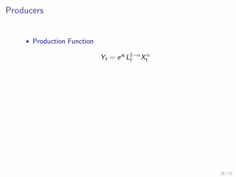
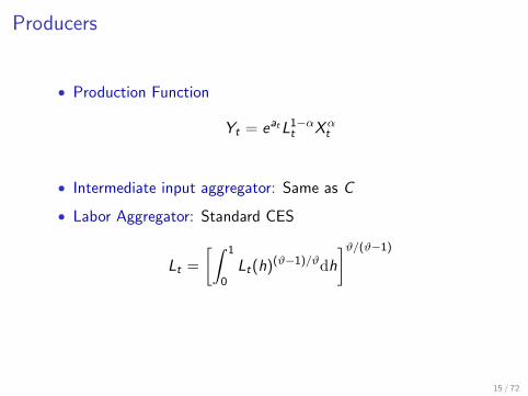
Producers
• Production Function
Yt = eatL1−αt Xα
t
• Intermediate input aggregator: Same as C
• Labor Aggregator: Standard CES
Lt =
[∫ 1
0Lt(h)(ϑ−1)/ϑdh
]ϑ/(ϑ−1)
15 / 72
Producers
• Production Function
Yt = eatL1−αt Xα
t
• Intermediate input aggregator: Same as C
• Labor Aggregator: Standard CES
Lt =
[∫ 1
0Lt(h)(ϑ−1)/ϑdh
]ϑ/(ϑ−1)
15 / 72

Producers
• Production Function
Yt = eatL1−αt Xα
t
• Intermediate input aggregator: Same as C
• Labor Aggregator: Standard CES
Lt =
[∫ 1
0Lt(h)(ϑ−1)/ϑdh
]ϑ/(ϑ−1)
15 / 72
ProducersOptimality Conditions
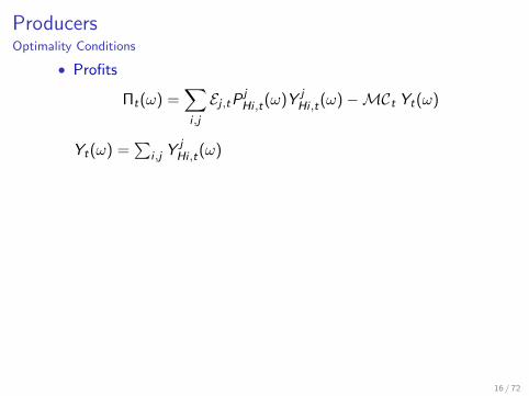
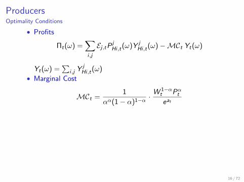
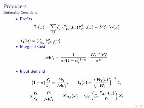
• Profits
Πt(ω) =∑i ,j
Ej ,tPjHi ,t(ω)Y j
Hi ,t(ω)−MCt Yt(ω)
Yt(ω) =∑
i ,j YjHi ,t(ω)
• Marginal Cost
MCt =1
αα(1− α)1−α ·W 1−α
t Pαteat
• Input demand
(1− α)Yt
Lt=
Wt
MCt, Lt(h) =
(Wt(h)
Wt
)−ϑLt
αYt
Xt=
Pt
MCtXiH,t(ω) = γiψ
(Dt
PiH,t(ω)
Pt
)Xt
16 / 72
ProducersOptimality Conditions
• Profits
Πt(ω) =∑i ,j
Ej ,tPjHi ,t(ω)Y j
Hi ,t(ω)−MCt Yt(ω)
Yt(ω) =∑
i ,j YjHi ,t(ω)
• Marginal Cost
MCt =1
αα(1− α)1−α ·W 1−α
t Pαteat
• Input demand
(1− α)Yt
Lt=
Wt
MCt, Lt(h) =
(Wt(h)
Wt
)−ϑLt
αYt
Xt=
Pt
MCtXiH,t(ω) = γiψ
(Dt
PiH,t(ω)
Pt
)Xt
16 / 72
ProducersOptimality Conditions
• Profits
Πt(ω) =∑i ,j
Ej ,tPjHi ,t(ω)Y j
Hi ,t(ω)−MCt Yt(ω)
Yt(ω) =∑
i ,j YjHi ,t(ω)
• Marginal Cost
MCt =1
αα(1− α)1−α ·W 1−α
t Pαteat
• Input demand
(1− α)Yt
Lt=
Wt
MCt, Lt(h) =
(Wt(h)
Wt
)−ϑLt
αYt
Xt=
Pt
MCtXiH,t(ω) = γiψ
(Dt
PiH,t(ω)
Pt
)Xt
16 / 72
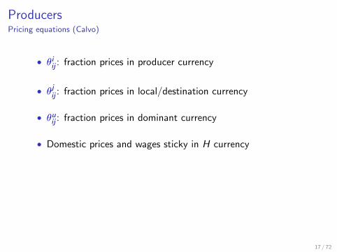
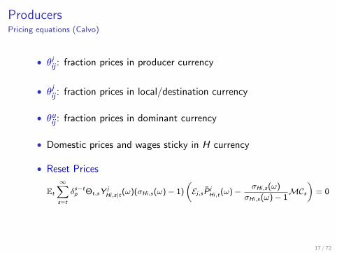
ProducersPricing equations (Calvo)
• θiij : fraction prices in producer currency
• θjij : fraction prices in local/destination currency
• θuij : fraction prices in dominant currency
• Domestic prices and wages sticky in H currency
• Reset Prices
Et
∞∑s=t
δs−tp Θt,sY
jHi,s|t(ω)(σHi,s (ω)− 1)
(Ej,s P
jHi,t(ω)− σHi,s (ω)
σHi,s (ω)− 1MCs
)= 0
17 / 72
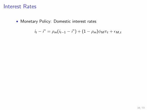
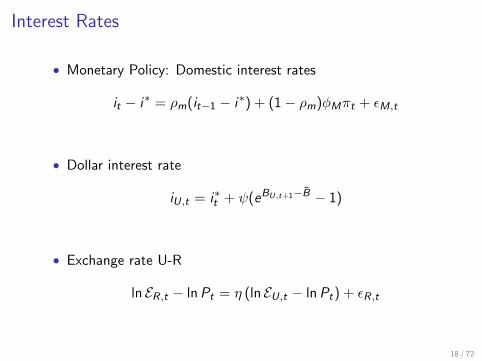
Interest Rates
• Monetary Policy: Domestic interest rates
it − i∗ = ρm(it−1 − i∗) + (1− ρm)φMπt + εM,t
• Dollar interest rate
iU,t = i∗t + ψ(eBU,t+1−B − 1)
• Exchange rate U-R
ln ER,t − lnPt = η (ln EU,t − lnPt) + εR,t
18 / 72

Interest Rates
• Monetary Policy: Domestic interest rates
it − i∗ = ρm(it−1 − i∗) + (1− ρm)φMπt + εM,t
• Dollar interest rate
iU,t = i∗t + ψ(eBU,t+1−B − 1)
• Exchange rate U-R
ln ER,t − lnPt = η (ln EU,t − lnPt) + εR,t
18 / 72
Interest Rates
• Monetary Policy: Domestic interest rates
it − i∗ = ρm(it−1 − i∗) + (1− ρm)φMπt + εM,t
• Dollar interest rate
iU,t = i∗t + ψ(eBU,t+1−B − 1)
• Exchange rate U-R
ln ER,t − lnPt = η (ln EU,t − lnPt) + εR,t
18 / 72
Exchange Rate Pass-through
• Export price pass-through in H currency higher• Greater the variability of mark-ups• Greater the reliance on imported inputs
• Import price pass-through in H currency lower• Greater the variability of mark-ups
19 / 72
Exchange Rate Pass-through
• Export price pass-through in H currency higher• Greater the variability of mark-ups• Greater the reliance on imported inputs
• Import price pass-through in H currency lower• Greater the variability of mark-ups
19 / 72
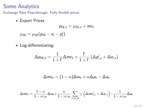
Some AnalyticsExchange Rate Pass-through: Fully flexible prices
• Export PricespHi ,t = µHi ,t + mct
µHi = µHi (pHi − ei − pii )
• Log-differentiating:
∆pHi ,t =1
1 + Γ∆mct +
Γ
1 + Γ
(∆pi
i ,t + ∆ei ,t
)
∆mct = (1− α)∆wt + α∆pt −∆at
∆mct =1− α
1− αγH∆wt +
α
1− αγH
∑i∈U,R
γi
(∆mc i
i,t + ∆ei,t
)− 1
1− αγH∆at
20 / 72
Some AnalyticsExchange Rate Pass-through: Fully flexible prices
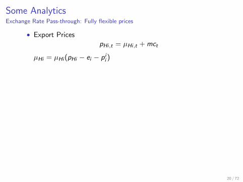
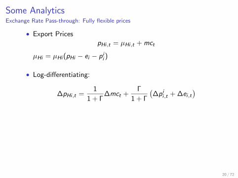
• Export PricespHi ,t = µHi ,t + mct
µHi = µHi (pHi − ei − pii )
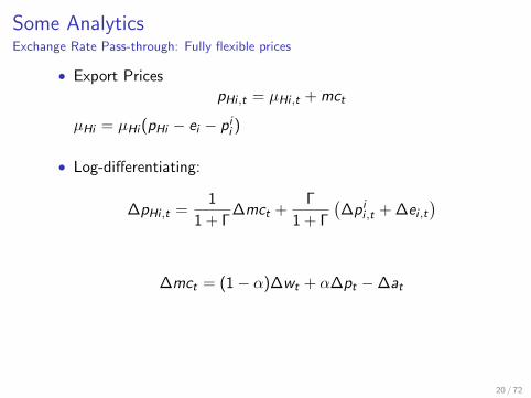
• Log-differentiating:
∆pHi ,t =1
1 + Γ∆mct +
Γ
1 + Γ
(∆pi
i ,t + ∆ei ,t
)
∆mct = (1− α)∆wt + α∆pt −∆at
∆mct =1− α
1− αγH∆wt +
α
1− αγH
∑i∈U,R
γi
(∆mc i
i,t + ∆ei,t
)− 1
1− αγH∆at
20 / 72
Some AnalyticsExchange Rate Pass-through: Fully flexible prices
• Export PricespHi ,t = µHi ,t + mct
µHi = µHi (pHi − ei − pii )
• Log-differentiating:
∆pHi ,t =1
1 + Γ∆mct +
Γ
1 + Γ
(∆pi
i ,t + ∆ei ,t
)
∆mct = (1− α)∆wt + α∆pt −∆at
∆mct =1− α
1− αγH∆wt +
α
1− αγH
∑i∈U,R
γi
(∆mc i
i,t + ∆ei,t
)− 1
1− αγH∆at
20 / 72
Some AnalyticsExchange Rate Pass-through: Fully flexible prices
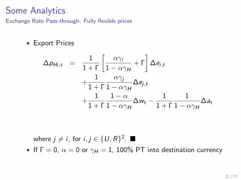
• Export Prices
∆pHi ,t =1
1 + Γ
[αγi
1− αγH+ Γ
]∆ei ,t
+1
1 + Γ
αγj
1− αγH∆ej ,t
+1
1 + Γ
1− α1− αγH
∆wt −1
1 + Γ
1
1− αγH∆at
where j 6= i , for i , j ∈ U,R2.
• If Γ = 0, α = 0 or γH = 1, 100% PT into destination currency
21 / 72
Some AnalyticsExchange Rate Pass-through: Fully flexible prices
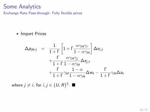
• Import Prices
∆piH,t =1
1 + Γ
[1 + Γ
αγHγi
1− αγH
]∆ei ,t
+Γ
1 + Γ
αγHγj
1− αγH∆ej ,t
+Γ
1 + ΓγH
1− α1− αγH
∆wt −Γ
1 + ΓγH∆at
where j 6= i , for i , j ∈ U,R2.
22 / 72
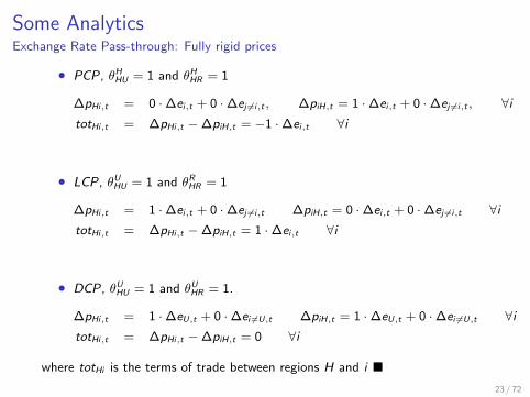
Some AnalyticsExchange Rate Pass-through: Fully rigid prices
• PCP, θHHU = 1 and θH
HR = 1
∆pHi,t = 0 ·∆ei,t + 0 ·∆ej 6=i,t , ∆piH,t = 1 ·∆ei,t + 0 ·∆ej 6=i,t , ∀itotHi,t = ∆pHi,t −∆piH,t = −1 ·∆ei,t ∀i
• LCP, θUHU = 1 and θR
HR = 1
∆pHi,t = 1 ·∆ei,t + 0 ·∆ej 6=i,t ∆piH,t = 0 ·∆ei,t + 0 ·∆ej 6=i,t ∀itotHi,t = ∆pHi,t −∆piH,t = 1 ·∆ei,t ∀i
• DCP, θUHU = 1 and θU
HR = 1.
∆pHi,t = 1 ·∆eU,t + 0 ·∆ei 6=U,t ∆piH,t = 1 ·∆eU,t + 0 ·∆ei 6=U,t ∀itotHi,t = ∆pHi,t −∆piH,t = 0 ∀i
where totHi is the terms of trade between regions H and i
23 / 72
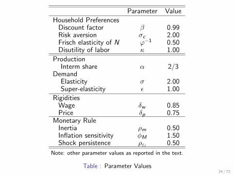
Parameter Value
Household PreferencesDiscount factor β 0.99Risk aversion σc 2.00Frisch elasticity of N ϕ−1 0.50Disutility of labor κ 1.00
ProductionInterm share α 2/3
DemandElasticity σ 2.00Super-elasticity ε 1.00
RigiditiesWage δw 0.85Price δp 0.75
Monetary RuleInertia ρm 0.50Inflation sensitivity φM 1.50Shock persistence ρεi 0.50
Note: other parameter values as reported in the text.
Table : Parameter Values24 / 72
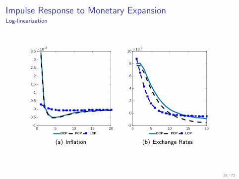
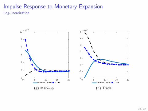
Impulse Response to Monetary ExpansionLog-linearization
0 5 10 15 20
#10-3
-1
-0.5
0
0.5
1
1.5
2
2.5
3
3.5
DCP PCP LCP
(a) Inflation
0 5 10 15 20
#10-3
-2
0
2
4
6
8
10
DCP PCP LCP
(b) Exchange Rates
25 / 72
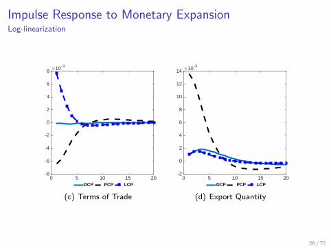
Impulse Response to Monetary ExpansionLog-linearization
0 5 10 15 20
#10-3
-8
-6
-4
-2
0
2
4
6
8
DCP PCP LCP
(c) Terms of Trade
0 5 10 15 20
#10-3
-2
0
2
4
6
8
10
12
14
DCP PCP LCP
(d) Export Quantity
26 / 72
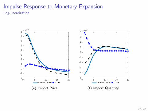
Impulse Response to Monetary ExpansionLog-linearization
0 5 10 15 20
#10-3
-2
-1
0
1
2
3
4
5
6
7
8
DCP PCP LCP
(e) Import Price
0 5 10 15 20
#10-3
-5
-4
-3
-2
-1
0
1
2
3
4
DCP PCP LCP
(f) Import Quantity
27 / 72
Impulse Response to Monetary ExpansionLog-linearization
0 5 10 15 20
#10-3
-2
0
2
4
6
8
10
DCP PCP LCP
(g) Mark-up
0 5 10 15 20
#10-3
-2
-1
0
1
2
3
4
5
DCP PCP LCP
(h) Trade
28 / 72
Colombia
• 2005-2014, Source: DIAN/DANE (customs), SIREM (agencysupervising large private firms
• Commodity Currency, Free float since September 1999
• Share of mining output in exports is 58.4%, Manufacturing,36.9%
• Currency composition of exports: USD: 98.4%
• Weighted (by income) average imported input share: 38% formanufacturers, 44% for manuf exporters
• Focus on manufacturing
29 / 72
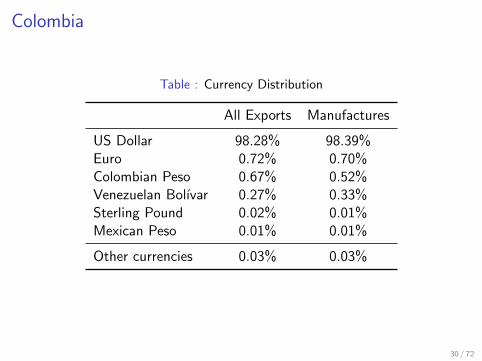
Colombia
Table : Currency Distribution
All Exports Manufactures
US Dollar 98.28% 98.39%Euro 0.72% 0.70%Colombian Peso 0.67% 0.52%Venezuelan Bolıvar 0.27% 0.33%Sterling Pound 0.02% 0.01%Mexican Peso 0.01% 0.01%
Other currencies 0.03% 0.03%
30 / 72
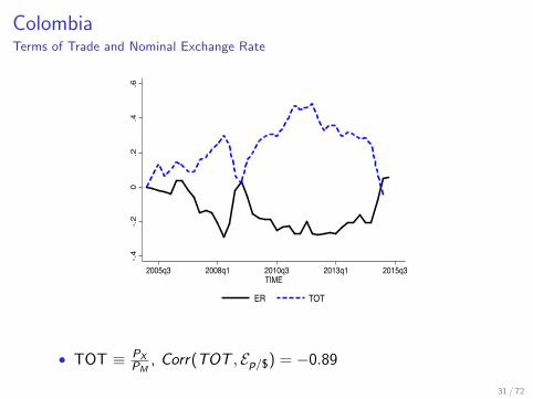
ColombiaTerms of Trade and Nominal Exchange Rate
-.4-.2
0.2
.4.6
2005q3 2008q1 2010q3 2013q1 2015q3TIME
ER TOT
• TOT ≡ PXPM
, Corr(TOT , Ep/$) = −0.89
31 / 72
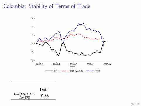
Colombia: Stability of Terms of Trade
-.4-.2
0.2
.4.6
2005q3 2008q1 2010q3 2013q1 2015q3TIME
ER TOT (Manuf) TOT
DataCov(ER,TOT )
Var(ER) -0.33
32 / 72
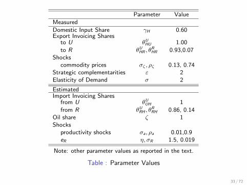
Parameter Value
Measured
Domestic Input Share γH 0.60Export Invoicing Shares
to U θUHU 1.00
to R θUHR , θ
RHR 0.93,0.07
Shockscommodity prices σζ , ρζ 0.13, 0.74
Strategic complementarities ε 2Elasticity of Demand σ 2
EstimatedImport Invoicing Shares
from U θUUH 1
from R θURH , θ
RRH 0.86, 0.14
Oil share ζ 1Shocks
productivity shocks σa, ρa 0.01,0.9eR η, σR 1.5, 0.019
Note: other parameter values as reported in the text.
Table : Parameter Values
33 / 72
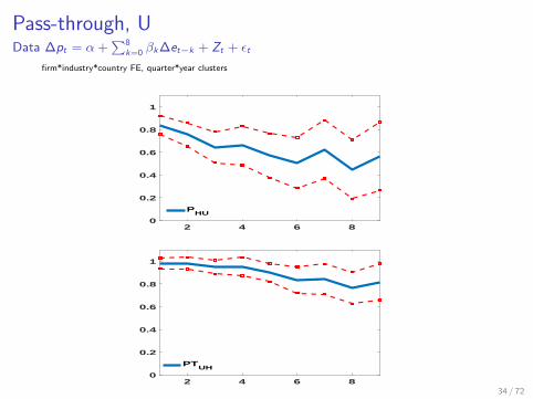
Pass-through, UData ∆pt = α +
∑8k=0 βk ∆et−k + Zt + εt
firm*industry*country FE, quarter*year clusters
2 4 6 80
0.2
0.4
0.6
0.8
1
PHU
2 4 6 80
0.2
0.4
0.6
0.8
1
PTUH
34 / 72
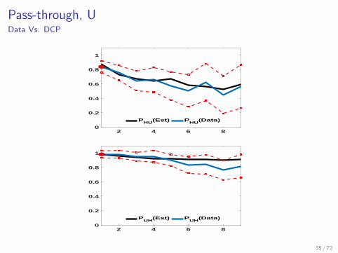
Pass-through, UData Vs. DCP
2 4 6 80
0.2
0.4
0.6
0.8
1
PHU
(Est) PHU
(Data)
2 4 6 80
0.2
0.4
0.6
0.8
1
PUH
(Est) PUH
(Data)
35 / 72
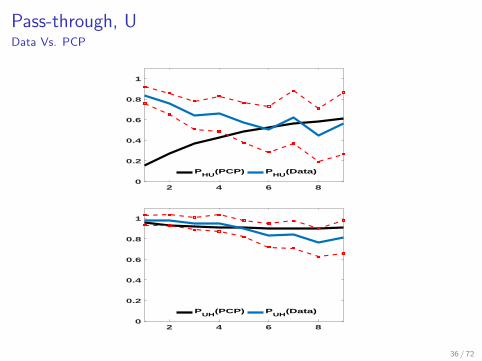
Pass-through, UData Vs. PCP
2 4 6 80
0.2
0.4
0.6
0.8
1
PHU
(PCP) PHU
(Data)
2 4 6 80
0.2
0.4
0.6
0.8
1
PUH
(PCP) PUH
(Data)
36 / 72
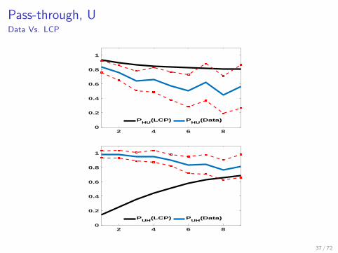
Pass-through, UData Vs. LCP
2 4 6 80
0.2
0.4
0.6
0.8
1
PHU
(LCP) PHU
(Data)
2 4 6 80
0.2
0.4
0.6
0.8
1
PUH
(LCP) PUH
(Data)
37 / 72
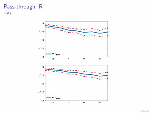
Pass-through, RData
2 4 6 8-1
-0.5
0
0.5
1
PTHR
2 4 6 8-1
-0.5
0
0.5
1
PTRH
38 / 72
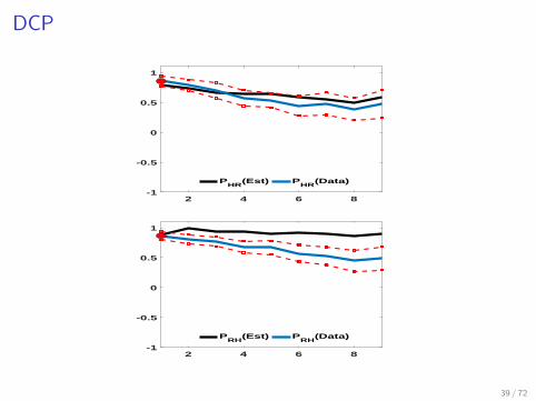
DCP
2 4 6 8-1
-0.5
0
0.5
1
PHR
(Est) PHR
(Data)
2 4 6 8-1
-0.5
0
0.5
1
PRH
(Est) PRH
(Data)
39 / 72
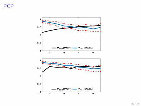
PCP
2 4 6 8-1
-0.5
0
0.5
1
PHR
(PCP) PHR
(Data)
2 4 6 8-1
-0.5
0
0.5
1
PRH
(PCP) PRH
(Data)
40 / 72
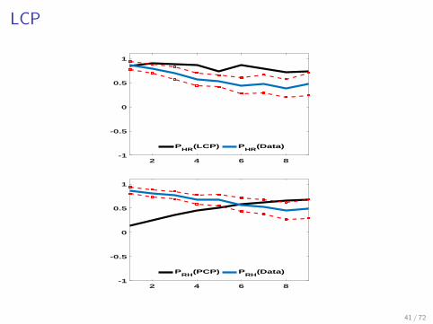
LCP
2 4 6 8-1
-0.5
0
0.5
1
PHR
(LCP) PHR
(Data)
2 4 6 8-1
-0.5
0
0.5
1
PRH
(PCP) PRH
(Data)
41 / 72
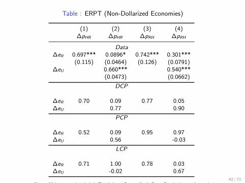
Table : ERPT (Non-Dollarized Economies)
(1) (2) (3) (4)∆pHR ∆pHR ∆pRH ∆pRH
Data∆eR 0.697*** 0.0896* 0.742*** 0.301***
(0.115) (0.0464) (0.126) (0.0791)∆eU 0.660*** 0.540***
(0.0473) (0.0662)
DCP
∆eR 0.70 0.09 0.77 0.05∆eU 0.77 0.90
PCP
∆eR 0.52 0.09 0.95 0.97∆eU 0.56 -0.03
LCP
∆eR 0.71 1.00 0.78 0.03∆eU -0.02 0.67
Notes: All data regressions include Firm-Industry-Country fixed effects. Standard errors clusteredat the year level. The sample includes manufactured products excluding petrochemicals and metalindustries. The export destinations include all countries except the Dollarized economies (USA,Panama, Puerto Rico, Ecuador, and El Salvador), economies with currencies pegged to the dollar,and Venezuela. Columns (3) and (6) exclude euro destinations. ‘***’, ‘**’, and ‘*’ indicatesignificance at the 1, 5, and 10 percent level, respectively.
42 / 72
Conclusion
• Most trade is invoiced in very few currencies.
• Dominant currency paradigm• pricing in a dominant currency• pricing complementarities• imported input use in production
• Data rejects PCP/LCP in favor of DCP.
• Implications• MP has limited impact on exports and terms of trade.
• TB adjusts mainly through exports not imports
• Adverse shock in emerging markets reduces world trade
• Inflation and imports sensitivity to DC exchange rates farexceeds the share of the dominant currency country in trade
43 / 72