Supply and Demand - About people.tamu.edupeople.tamu.edu/~aglass/econ323/Chapter02Slides.pdf · Supply and Demand Curves • A Market: consists of the buyers and sellers of a good

Chapter 2

Supply and Demand

Chapter Outline• Supply and Demand Curves• Equilibrium Quantity and Price• Excess Supply, Excess Demand, and Adjustment to Equilibrium

• Some Welfare Properties of Equilibrium• Free Markets and The Poor

– Rent Controls and Price Supports– The Rationing and Allocative Function of Prices

• Determinants of Supply and Demand• How Taxes Affect Equilibrium Prices

©2015 McGraw‐Hill Education. All Rights Reserved. 2

Supply and Demand Curves

• A Market: consists of the buyers and sellers of a good or service.

• Law of Demand: the empirical observation that when the price of a product falls, people demand larger quantities of it.

• Law of Supply: the empirical observation that when the price of a product rises, firms offer more of it for sale.


Figure 2.1: A Demand Curve P=24‐4Q


Figure 2.2: A Supply Curve P=4Q


Equilibrium Quantity and Price• Equilibrium quantity and price: it is the price‐quantity pair at which both buyers and sellers are satisfied.

• Excess supply: the amount by which quantity supplied exceeds quantity demanded.

• Excess demand: the amount by which quantity demanded exceeds quantity supplied.


Figure 2.3: Equilibrium Q=3000, P=$12


Figure 2.4: Excess Supply and Excess Demand


Some Welfare Properties of Equilibrium

• If price and quantity take anything other than their equilibrium values, however, it will always be possible to reallocate so as to make at least some people better off without harming others.

• If P=$8 and quantity supplied is only 2,000, people are willing to pay up to $16 for an additional unit so more should be sold.


Figure 2.5: An Opportunity for Improvement


Free Markets and the Poor

• Efficiency says that given the low incomes of the poor, free exchange enables them to do the best they can.

• Price ceilings attempting to make goods more affordable can make items less available.

• Price supports cause excess supply that the government usually has to buy.


Rent Controls


• A price ceiling for rents is a level beyond which rents are not permitted to rise.

• Rent controls increase quantity demanded and decrease quantity supplied, causing excess demand.

Rent Controls


• In Figure 2.6, limiting rent to $400/month (rather than the market rate of $600) creates an excess demand of 40,000 units.

• 80,000 units are demanded but only 40,000 are supplied.

• No guarantee that the 40,000 units available will go to the renters who value the units the most.

Figure 2.6: Rent Controls


Price Supports


• A price support (or price floor) keep prices above their equilibrium levels.

• Requires the government to become an active buyer in the market to buy up the excess supply that stems from the artificially high price.

• Purpose of farm price supports is to ensure prices high enough to provide adequate incomes for farm families.– May be better to transfer money in other ways.

Price Supports

• The equilibrium in this soybean market should be P=$300/ton and Q=300,000 tons/yr.

• The government places a price support (price floor) of P=$400/ton in an attempt to raise the incomes of soybean farmers.

• Quantity supplied increases to 400,000 tons/yr while quantity demanded falls to 200,000, causing excess supply of 200,000 for the government to buy.


Price Supports

• At equilibrium P=$300/ton and Q=300,000 tons/yr, revenues would be $90,000,000/yr.

• At P=$400/ton and Q=200,000, soybean revenues would fall to $80,000,000/yr.

• If the government buys up the excess supply, then soybean revenue would rise to 160,000,000/yr but half of that is what the government paid for the excess supply.

• Should consider letting the market set the price and gifting to farmers the $80,000,000 that would have spent on buying the excess soybeans.


Figure 2.7: A Price Support in the Soybean Market


The Rationing and Allocative Functions of Prices

• Rationing function of price: the process whereby price directs existing supplies of a product to the users who value it most highly.

• Allocative function of price: the process whereby price acts as a signal that guides resources away from the production of goods whose prices lie below cost toward the production of goods whose prices exceed cost.


Factors the Shift the Demand Curve

• Incomes– Normal goods: the quantity demanded at any price rises with income.

– Inferior goods: the quantity demanded at any price falls with income.

• Tastes• Price of Substitutes and Complements

– Complements ‐ an increase in the price of one good decreases demand for the other good.

– Substitutes ‐ an increase in the price of one will tend to increase the demand for the other.

• Expectations• Populations


Figure 2.8: Factors that ShiftDemand Curves


Factors the Shift the Supply Curve

• Technology

• Factor Prices

• The Number of Suppliers

• Expectations

• Weather


Figure 2.9: Factors that Shift Supply Schedules


Predicting Changes in Price and Quantity

• An increase in demand → an increase in both the equilibrium price and quantity.

• A decrease in demand → a decrease in both the equilibrium price and quantity.

• An increase in supply → a decrease in the equilibrium price and an increase in the equilibrium quantity.

• A decrease in supply → an increase in the equilibrium price and a decrease in the equilibrium quantity.


Predicting Changes in Price and Quantity

• Agricultural products, such as apples, see a seasonal increase in supply, which leads to a decrease in the equilibrium price and an increase in the equilibrium quantity.

• Some products, such as beachfront cottages, see a seasonal increase in demand, which leads to an increase in both the equilibrium price and quantity.


Figure 2.10: Two Sources of Seasonal Variation


Figure 2.11: The Effect of Soybean Price Supports on the Equilibrium Price and Quantity of Beef


The Algebra of Supply and Demand

• For computing numerical values, it is more convenient to find equilibrium prices and quantities algebraically– The supply schedule is: P= 2 + 3Qs

– Its demand schedule is: P = 10 – Qd

– In equilibrium we know that Qs = Qd, denoting this common value as Q*, we arrive at: 2 + 3Q* = 10 – Q*

– Which gives Q* = 2, substituting this back into either the supply or demand equation gives the equilibrium price, P* = 8


Figure 2.12: Graphs of the Supply and Demand Equations


Tax Burdens

• Starting from an equilibrium price P*, consider the effects of imposing a tax of T per unit sold.

• Let PB be the price paid by the buyer and PS be the price received by the seller.

• Initially, the buyer pays P* to the seller. With the tax, the buyer pays PB=PS+T to the seller, with the seller keeping only PS.


Tax Burdens

• The buyer’s share of the tax burden is how much the price paid by the buyer increases

relative to the size of the tax .

• The seller’s share of the tax burden is how much the price received by the seller decreases relative to the size of the tax

.


Figure A2.1: A Tax of T=10 Levied on the Seller Shifts the Supply Schedule Upward by T Units


Figure A2.2: Equilibrium Prices and Quantities When a Tax of T = 10 is Levied on the Seller


Figure A2.3: The Effect of a Tax of T = 10 Levied on the Buyer


Figure A2.4: Equilibrium Prices and Quantities after Imposition of a Tax of a Tax of T = 10 Paid by the Buyer


A Tax on the Buyer Leads to the Same Outcome as a Tax on the Seller

• Demand P=10‐Q, supply P=Q, T=2.

• Initial equilibrium P=5, Q=5.

• Impose tax on seller so P=T+Q=2+Q. 10‐Q=2+Q, 2Q=8, Q=4; PB=10‐Q=10‐4=6; PS=PB‐T=4

• Impose tax on buyer so P=10‐T‐Q=8‐Q.8‐Q=Q, 2Q=8, Q=4; PS=Q=4; PB=PS+T=4+2=6

• Same result either way. tB =tS =50%


Figure A2.5: A Tax on the Buyer Leads to the Same Outcome as a Tax on the Seller


Tax Burden

• If supply is perfectly inelastic (a vertical line at Q0), the full amount of the tax will go into the price that the seller receives going down and tS=100%.– Or if demand perfectly elastic (horizontal line at P0).

• If supply is perfectly elastic (a horizontal line at P0), the full amount of the tax will go into the price that the buyer pays going up and tB=100%.– Or if demand perfectly inelastic (vertical line at Q0).


Problem 1

1. Supply is P = 4Q, while demand is P = 20, where P is price in dollars and Q is units of output per week. Find and graph the equilibrium price and quantity. If sellers must pay a tax of T = $4/unit, what happens to the quantity exchanged, the price buyers pay, and the price sellers receive (net of the tax)? How is the burden of the tax distributed across buyers and sellers and why?


Solution 1

1. Initial equilibrium price P*=$20; 20=4Q, Q*=5. With the tax, the supply curve shifts up by T=4 to P=4+4Q; buyers pay only PB=$20; 20=4+4Q, 4Q=16, Q=4 units transacted (one less than before); sellers receive what the buyers pay minus the tax PS=PB‐T=20‐4=$16. Sellers suffer the full tax burden due to demand being perfectly elastic.


Solution 1 Figure

S’

S

4 5

20

40


D

Problem 2

2. Repeat, but instead assume the buyer pays the tax, demand is P = 28 ‐ Q and supply is P = 20.


Solution 2

2. Initial equilibrium price P*=$20; 28‐Q=20, Q*=8. With the tax, the demand curve shifts down by T=4 to P=28‐4‐Q=24‐Q. Sellers must receive PS=$20. 20=24‐Q; Q=4 quantity transacted. Buyers pay what the sellers receive plus the tax PB=PS+T=20+4=$24. Buyers suffer the full tax burden due to supply being perfectly elastic.


Solution 2 Figure

0

20

0 8

28

24

4

S

D

D’


Problem 3

3. Suppose demand for football games is P = 1900 ‐ (1/50) Q and supply is fixed at Q = 90,000 seats. Find the equilibrium price and quantity of seats for a football game. Suppose the government prohibits ticket scalping (selling tickets above their face value), and the face value of tickets is $50 (this policy places a price ceiling at $50). How many consumer will be dissatisfied (how large is excess demand)? Suppose the next game is a major rivalry, and so demand jumps to P = 2100 ‐ (1/50)Q. How many consumers will be dissatisfied for the big game? How do the distortions of this price ceiling differ from the more typical case of upward sloping supply?


Solution 3

3. Initial equilibrium price P*=1900‐90000/50=1900‐1800=$100; quantity Q*=90,000. Quantity supplied is fixed at Q=90,000. With a price ceiling of $50, 50=1900‐Q/50, Q/50=1850, QD=92,500 quantity demanded. Excess demand QD‐QS=92,500‐90,000=2,500 consumers dissatisfied because they cannot find a ticket to buy. For the big game 50=2100‐Q/50, Q/50=2050, QD=102,500 quantity demanded. Excess demand grows to QD‐QS=102,500‐90,000=12,500. The distortions of this price ceiling are all on the demand side since quantity supplied does not adjust.


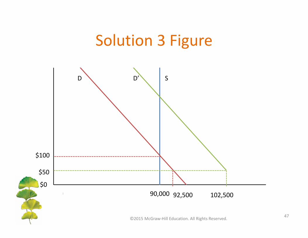
Solution 3 Figure

$070,000 90,000

$100

$50

92,500 102,500

D D’ S


Problem 4

4. Suppose the supply of a good is P = Q and demand is fixed at Q = 12 units per week. Find the equilibrium price and quantity. Suppose the government levies a tax equal to $4 on sellers of the good. Find the quantity exchanged, price paid by buyers, and price received by sellers (net of taxes). How is the tax burden distributed and why?


Solution 4

4. Initial equilibrium price P*=Q=$12; Q*=12. With the tax on sellers, the supply curve shifts up by T=4 to P=T+Q=4+Q=4+12=16. PB=$16, PS=PB‐T=16‐4=$12. Buyers suffer the full tax burden due to demand being perfectly inelastic.


Solution 4 Figure

0

4

8

12

16

0 12

D S’ S


Documents

Supply and Demand - About people.tamu.edupeople.tamu.edu/~aglass/econ323/Chapter02Slides.pdf · Supply and Demand Curves • A Market: consists of the buyers and sellers of a good