Embed Size (px)
Citation preview
4 Inflation modelling in the euro area
Fabio C. Bagliano, Roberto Golinelliand Claudio Morana
1 Introduction
Controlling inflation, at least in the long run, is widely regarded as the primary,and sometimes the only, goal of monetary policy. To this aim, in many coun-tries central banks have explicitly adopted inflation-targeting strategies, settingprecise quantitative targets for the monetary authorities’ actions. Though notan inflation targeter, the European Central Bank (ECB) adopted a monetarypolicy strategy aimed at maintaining an annual inflation rate below 2% overa medium-term horizon (ECB 1999). This strategy is based on an announcedreference value for M3 money growth and on the outlook of price developmentsin the euro area. The analysis of the behaviour of monetary aggregates and theircomponents relies on a number of tools recently summarised in ECB (2001).The aim of this chapter is to provide an empirical investigation of the inter-relationships among money, prices, interest rates and output in the euro areawith a particular focus on the behaviour of the inflation rate over a long-runhorizon. In fact, one of the main open issues in inflation analysis stems fromthe fact that short-run fluctuations of the observed inflation rate may be dueto only temporary disturbances to which monetary policy should not respond.How to construct a reliable empirical measure of the underlying, long-run trendof inflation – ‘core’ inflation – has therefore become a crucial issue in monetarypolicy design.
Core inflation series have been constructed following different methodolo-gies (see Wynne 1999 for a thorough overview and assessment of differentmeasures). Some measures are obtained from the cross-sectional distributionof individual price items, either by excluding from the price index some cat-egories of goods (such as energy and food items) which are believed to behigh-variance components, or by computing more efficient, ‘limited influence’
This paper was originally prepared for the EMU Macroeconomic Institutions Conference, Uni-versita di Milano-Bicocca, 20–22 September 2001. We thank our discussant, Gianni Amisano,conference participants, and Steven Durlauf for many useful comments. Financial support fromMIUR (F. C. Bagliano and R. Golinelli) and CNR (F. C. Bagliano) is gratefully acknowledged.
59
60 F. C. Bagliano, R. Golinelli and C. Morana
estimators of the central tendency of the distribution, such as the (weighted)median popularised by Bryan and Cecchetti (1994) and Cecchetti (1997) for theUSA. Other measures are derived from univariate statistical techniques, suchas simple moving averages computed over a variable time span (from 3–6 up to36 months) or more sophisticated methodologies (i.e. unobserved componentmodels, or the one-sided low-pass filter proposed by Cogley 2002). Finally,Quah and Vahey (1995) applied to the UK a bivariate structural vector autore-gressive (SVAR) approach to core inflation estimation based on long-run outputneutrality of permanent shocks to the inflation rate.
We propose a different, explicitly forward-looking, measure of core inflation,based on (appropriately estimated and tested) long-run relations among majormacroeconomic variables. This measure may provide useful information in thelight of the ‘two-pillar’ monetary policy strategy of the ECB, which consid-ers: (i) the deviations of M3 growth from a reference value (a money growthindicator), and (ii) a broadly based assessment of the outlook for future pricedevelopments in the euro area as a whole (ECB 1999, 2000). This framework ismotivated by the (alleged) close long-run relationship between money growthand inflation. Recent results have provided some evidence of stable long-runrelationships among money, output, interest rates and inflation over the last twodecades for the EMU countries (Brand and Cassola 2000, Gerlach and Svensson2001, Golinelli and Pastorello 2002). We use such information to construct aforward-looking measure of core inflation consistent with the long-run featuresof the euro area macroeconomy.
To this aim, we consider a multivariate framework, capturing the dynamicinteractions among the inflation rate, real money balances, short- and long-term interest rates and output, extending the analysis in Bagliano, Golinelli andMorana (2002). A stylised macroeconomic model is set up in section 2 to pro-vide a theoretical rationale for the potential long-run relationships among thosevariables. The existence of valid cointegrating relations is then explored usingeuro area data for the 1979–2001 period. The problem of structural breaks in thebehaviour of the long-term real interest rate is addressed by means of a Markov-switching model for the real rate. In order to decompose observed inflation into anon-stationary (stochastic) trend component, capturing the effect of permanentshocks only, and a stationary transitory element, we adopt a common trendsapproach. The permanent, ‘core’ inflation component bears the interpretation ofthe long-run inflation forecast conditional on an information set including sev-eral important macroeconomic variables. The main advantage of this measureof core inflation lies in its forward-looking nature, capturing the long-term ele-ment of the inflation process (of particular interest from the monetary policy per-spective) consistent with the long-run properties of the macroeconomic system.Section 3 describes the common trends methodology and presents empirical re-sults. Several properties of the estimated core inflation process are then assessed,

Inflation modelling in the euro area 61
namely its relative volatility with respect to observed inflation and its abilityto forecast future headline inflation rates. Further features of the permanent-transitory decomposition of the inflation rate are analysed in section 4,where the nature of the non-core inflation fluctuations and the convergenceof the observed rate to the core inflation rate are discussed. Finally, our mainmessage is summarised in the concluding section 5: the ECB should take intoproper account a forward-looking measure of the core inflation rate consistentwith its whole monetary policy framework, based on strong and stable long-runrelationships between inflation and other major macroeconomic variables.
2 Long-run analysis of a small-scale macro system
To organise thinking about the long-run relationships among inflation, output,money and interest rates we start with a general equation for inflation determi-nation, nesting a traditional backward-looking Phillips curve, whereby inflationis mainly determined by the ‘output gap’, and a P* model (see Hallman, Porterand Small 1991), which assumes that inflation dynamics is governed by the‘price gap’. The latter model has recently received strong support for the euroarea from Gerlach and Svensson (2001). Ignoring additional dynamic termsand exogenous variables, the equation for the inflation rate is of the form:
πt = π et,t−1 + αy(yt−1 − y∗
t−1) + αm(pt−1 − p∗t−1) + επ
t , (4.1)
where π t is the annualised inflation rate in quarter t (π t ≡ 4(pt − pt−1)) andπ e
t,t−1 is the expected inflation rate as of quarter t − 1, y−y* measures the outputgap, with y* denoting potential output, and p − p* is the ‘price gap’, the keydeterminant of inflation in the P* model, to be more precisely defined below.Finally, επ represents a random shock to inflation. The empirical specification ofequation (4.1) requires us to model inflationary expectations. As in other studieswhich use a backward-looking Phillips curve (e.g. Taylor 1999, Rudebusch andSvensson 1999, Staiger, Stock and Watson 2001), the expected inflation rateπ e
t,t−1 is set equal to πt−1.1 Therefore we get:
� πt = αy(yt−1 − y∗t−1) + αm(pt−1 − p∗
t−1) + επt . (4.2)
Moreover, we assume:
y∗t = β
y0 + y∗
t−1 + εyt (4.3)
mt − pt = βm0 + βm
1 yt + βm2 (lt − st ) + εm
t (4.4)
p∗t = mt − [
βm0 + βm
1 y∗t + βm
2 (s∗t − l∗t )
](4.5)
1 Gerlach and Svensson (2001) adopt a different specification, setting π et,t−1 as a weighted average
of πt−1 and of the central bank’s inflation objective.

62 F. C. Bagliano, R. Golinelli and C. Morana
lt = βf
0 + π et+1,t + ε
ft (4.6)
lt = βs0 + st + εs
t . (4.7)
In (4.3) potential output follows a random walk. Real money demand is specifiedby (4.4), where the long–short interest rate differential (l − s) proxies theopportunity cost of money holdings. Equation (4.5) defines p∗
t as the pricelevel consistent with the current money stock, potential output and long-runequilibrium values for the short and long interest rates (s* and l*), according tothe P* model. Finally, (4.6) and (4.7) capture a Fisher parity and a term structurerelation respectively. All structural parameters (βs) are positive and the εs arerandom shocks. In a long-run equilibrium, the following relations hold:
y = y∗
π = π e
l∗ = βf
0 + π
l∗ = βs0 + s∗
m∗ − p∗ = β0 + βm1 y∗,
where m* denotes long-run equilibrium nominal money balances and β0 ≡βm
0 + βm2 βs
0 .
In the above framework, the inflation rate and output are non-stationary, I(1),and the output gap is stationary, I(0). Moreover, the long-term interest rateis I(1) and cointegrated with the inflation rate, so that l − π is I(0), and theshort-term rate is I(1) and cointegrated with the long rate, so as to make l − sstationary. From (4.4) real money balances are I(1) and cointegrated with output;if the cointegration parameter βm
1 �= 1, also money velocity is non-stationary.Then, the first step of our empirical analysis looks at the integration and coin-tegration properties of the series, to check their consistency with the abovemacroeconomic framework.
In order to proceed with the empirical analysis, we need euro-area variablesover a time span pre-dating the launch of the euro at the beginning of 1999. Forthe pre-euro period (up to 1998Q4) aggregate variables for the euro area wereconstructed by aggregating the historical data of the twelve current membercountries. This approach is based on the assumption that the artificial euro-areadata before monetary union are appropriate for analysing and forecasting thearea-wide behaviour under EMU.2
2 Despite this caveat, the aggregation route was followed by several other recent studies: Gerlachand Svensson (2001) and Galı, Gertler and Lopez-Salido (2001) recently used area-aggregateddata to study the EMU inflation rate, and Golinelli and Pastorello (2003) find some results infavour of the statistical poolability of single-country money demand functions. The latter resultsare partly supported by Dedola, Gaiotti and Silipo (2001), who find that the area-wide money

Inflation modelling in the euro area 63
In the present analysis, we use quarterly variables at an area-wide level overthe 1978Q4−2001Q3 period. We measure (the log of) real money balances(m − p) by the (log of the) index of nominal M3 (published by the ECB)deflated by the (log of the) Harmonised Index of Consumer Prices (HICP) usedby the ECB; output (y) is measured by (the log of) real GDP, the nominal shortand long-term interest rates (s and l) are the T-bill and the government bondrates, the inflation rate (π ) is the annualised quarterly rate of change of the HICP,and the output gap (ygap ≡ y − y *) is measured by the rate of capacity utilisationin the manufacturing sector measured by the OECD.3
The results of unit-root Dickey-Fuller ADF tests reported in table 4.1 areclear-cut: with the only exception of ygap, which is stationary, all the variablesof interest are first order integrated. Moreover, the lower part of the table reportsADF test statistics for a number of additional variables: if the (null) unit-roothypothesis is rejected, then the corresponding I(1) series are cointegrated witha (1, −1) cointegrating vector. The results show that money velocity is I(1) evenwhen a linear trend is allowed in the specification of the test, the term interest ratedifferential is stationary (short and long-term rates are cointegrated), whereasthe short- and long-term real interest rates are not stationary. As a whole, theevidence is consistent with the features of the above theoretical framework,except for the behaviour of the real interest rate series.
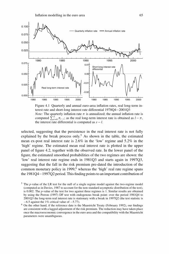
The missing Fisher parity relation deserves more careful scrutiny. To thisaim, the lower panel of figure 4.1 plots the long-term real (ex-post) interestrate and the term interest rate differential for the euro area over the whole1978Q4−2001Q3 period. While the interest rate differential fluctuates quitepersistently around a constant mean, the real long-term interest rate shows amuch lower mean for the sub-periods 1978–81 and 1997–2001, possibly sug-gesting that the non-stationarity detected by the ADF test is spurious, anddue to a neglected structural change in the constant term of the Fisher par-ity relation.4 For example, the introduction of the single monetary policy ex-plicitly aimed at a price stability objective may have reduced inflation uncer-tainty and therefore the inflation risk premium embodied in the level of the
demand equation is not significantly affected by aggregation bias. Brand and Cassola (2000) andCoenen and Vega (2001) also study money demand only at an area-wide level. On the other side,Marcellino, Stock and Watson (2003), and Espasa, Albacete and Senra (2002) provide evidenceagainst the use of aggregate models and prefer to forecast a number of euro-area variables atcountry level. Against this view, Bodo, Golinelli and Parigi (2000) show that the area-wide modelis better than single country models in forecasting industrial production. Finally, a completelydifferent approach is followed by Rudebusch and Svensson (2002), who use a model estimatedon US data to discuss euro-area policy issues.
3 The data used in the empirical analysis are updated from Golinelli and Pastorello (2002). Thedata set is available for downloading at http://www.spbo.unibo.it/pais/golinelli/macro.htm, wherefurther details on the sources are also provided.
4 Moreover, the Hansen (1992) instability test confirms the presence of instability in the mean realinterest rate at the 5% significance level (Lc = 1.40).
64 F. C. Bagliano, R. Golinelli and C. Morana
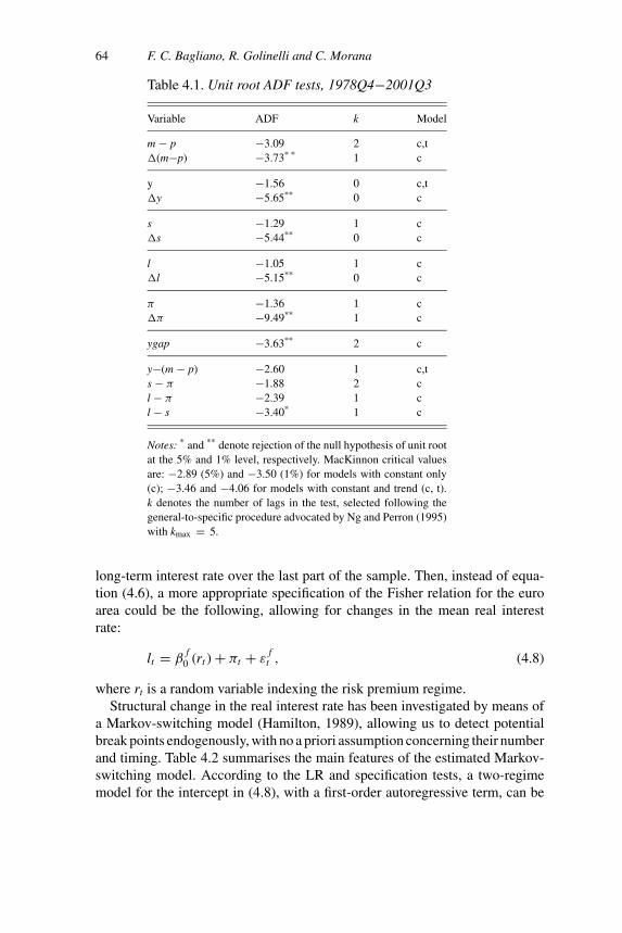
Table 4.1. Unit root ADF tests, 1978Q4−2001Q3
Variable ADF k Model
m − p −3.09 2 c,t�(m−p) −3.73* * 1 c
y −1.56 0 c,t�y −5.65** 0 c
s −1.29 1 c�s −5.44** 0 c
l −1.05 1 c�l −5.15** 0 c
π −1.36 1 c�π −9.49** 1 c
ygap −3.63** 2 c
y−(m − p) −2.60 1 c,ts − π −1.88 2 cl − π −2.39 1 cl − s −3.40* 1 c
Notes: * and ** denote rejection of the null hypothesis of unit rootat the 5% and 1% level, respectively. MacKinnon critical valuesare: −2.89 (5%) and −3.50 (1%) for models with constant only(c); −3.46 and −4.06 for models with constant and trend (c, t).k denotes the number of lags in the test, selected following thegeneral-to-specific procedure advocated by Ng and Perron (1995)with kmax = 5.
long-term interest rate over the last part of the sample. Then, instead of equa-tion (4.6), a more appropriate specification of the Fisher relation for the euroarea could be the following, allowing for changes in the mean real interestrate:
lt = βf
0 (rt ) + πt + εf
t , (4.8)
where rt is a random variable indexing the risk premium regime.Structural change in the real interest rate has been investigated by means of
a Markov-switching model (Hamilton, 1989), allowing us to detect potentialbreak points endogenously, with no a priori assumption concerning their numberand timing. Table 4.2 summarises the main features of the estimated Markov-switching model. According to the LR and specification tests, a two-regimemodel for the intercept in (4.8), with a first-order autoregressive term, can be
Inflation modelling in the euro area 65
1980 1985 1990 1995 2000
0.025
0.050
0.075
0.100
Quarterly inflation rate Annual inflation rate
1980 1985 1990 1995 2000
0.000
0.025
0.050
0.075
Real long-term interest rate
1980 1985 1990 1995 2000
−0.02
−0.01
0.00
0.01Short-long interest ratedifferential
Figure 4.1 Quarterly and annual euro-area inflation rates, real long-term in-terest rate and short-long interest rate differential 1978Q4−2001Q3Note: The quarterly inflation rate π is annualized; the annual inflation rate iscomputed
∑3i=0 πt−i ; as the real long-term interest rate is obtained as l − π ,
the interest rate differential is computed as s − l.
selected, suggesting that the persistence in the real interest rate is not fullyexplained by the break process only.5 As shown in the table, the estimatedmean ex-post real interest rate is 2.6% in the ‘low’ regime and 5.2% in the‘high’ regime. The estimated mean real interest rate is plotted in the upperpanel of figure 4.2, together with the observed rate. In the lower panel of thefigure, the estimated smoothed probabilities of the two regimes are shown: the‘low’ real interest rate regime ends in 1981Q3 and starts again in 1997Q3,suggesting that the fall in the risk premium pre-dated the introduction of thecommon monetary policy in 1999,6 whereas the ‘high’ real rate regime spansthe 1981Q4−1997Q2 period. This finding points to an important contribution of
5 The p-value of the LR test for the null of a single regime model against the two-regime model(computed as in Davies, 1987 to account for the non-standard asymptotic distribution of the test),is 0.002. The p-value of the test for two against three regimes is 1. Similar results are obtainedby using the Perron (1997) DF test with endogenous break point: over the period 1981Q4 to2001Q3 the long-term real interest rate is stationary with a break in 1997Q2 (the test statistic is−6.5 against the 1% critical value of −5.77).
6 On the other hand, if the reference date is the Maastricht Treaty (February 1992), our findingsare consistent with a lagged adjustment of the risk premium. The reduction may have taken placeonce the macroeoconomic convergence in the euro area and the compatibility with the Maastrichtparameters were unambiguous.

66 F. C. Bagliano, R. Golinelli and C. Morana
Table 4.2. Regime switching analysis of the long-termreal interest rate.
Regime 1 Regime 2
Regime 1 0.952 0.016Regime 2 0.048 0.984
Mean 2.58 5.19(0.21) (0.13)
Duration (quarters) 21 61Number of observations 29 63
Notes: The first four rows of the table report the transition matrix(pij = Pr{r(t) = i / r(t − 1) = j}). Mean denotes the estimatedex-post real interest rate in the two regimes. Duration denotesthe average duration of each regime in quarters. The number ofobservations in each regime is reported in the last row.
1980 1985 1990 1995 2000
0.000
0.025
0.050
0.075
_ _ _ Real interest rate ___ Estimated mean real interest rate
1980 1985 1990 1995 2000
0.5
1.0Smoothed probability of the "high" real interest rate regime
Figure 4.2 Markov-switching model of real interest rate
monetary unification to economic growth, through a reduced cost of investmentfinancing.
The existence of two different regimes in the real interest rate behaviourhas relevant consequences for the long-run empirical modelling of our set ofsix variables of interest (m − p, y, s, l, π and ygap). In fact, when tests forthe cointegration rank and the forecasting ability are performed on a VAR(3)
Inflation modelling in the euro area 67
system over the 1981Q4−1997Q2 period only (identified above by the Markov-switching model as the ‘high’ real interest rate regime), the Johansen (1995)trace statistics support the existence of four cointegrating relationships at the10% significance level. However, the one-step (ex-post) parameter constancyforecast test over the period 1998–2001 reveals strong evidence of a signifi-cant shift and, accordingly, the cointegration test over the full sample detectsfewer than four cointegrating relationships. In short, the extension of the sampleperiod leads to forecast failure and missing cointegration owing to parameterinstability.
In order to capture the structural change in the long-run Fisher relation de-tected above, we include in the basic VAR system a step dummy variable (RP)taking the value of 1 during the ‘high’ real rate regime (1981Q4−1997Q2), and0 in the ‘low’ rate regime (1978Q4−1981Q3 and 1997Q3−2001Q3). Prior topresenting the results, the next subsection shows how the standard methodologyis extended to include a dummy variable in the cointegrating space.
2.1 Methodology
The standard vector error-correction mechanism (VECM) representation of themodel, controlling for a linear trend in the level of the variables, can be writtenas
Π∗(L) �xt = ν + Π(1) xt−1 + εt , (4.9)
where xt is the vector of n I(1) cointegrated variables of interest,ν is the vector ofintercept terms, εt ∼ N I D (0, �); Π(L) = In − ∑p
i=1 Πi Li , Π∗ (L) = In −∑p−1i=1 Π∗
i Li and Π∗i = − ∑p
j=i+1 Π j (i = 1, . . . , p − 1). If there are 0 < k< n cointegration relationships among the variables, Π(1) is of reduced rankk and can be expressed as the product of two (n × k) matrices: Π(1) =αβ′,where β contains the cointegrating vectors, such that β′xt are stationary linearcombinations of the I(1) variables, and α is the matrix of factor loadings.When one of the cointegrating vectors (i.e. the kth vector) contains a switchingintercept modelled by dummy variables, it is possible to rewrite the β matrixas
β(n+q)×k =
βn×k
0q×(k−1)
β∗q×1
,
whereβ* is the q × 1 subvector containing the parameters of the q deterministicvariables in the kth cointegrating vector. If there are q regimes, q − 1 regimesmay be normalised relative to the qth regime; this amounts to measuring theswitches relative to a constant intercept term, therefore requiring a constantterm and q − 1 intervention dummies. The VECM representation can then be
68 F. C. Bagliano, R. Golinelli and C. Morana
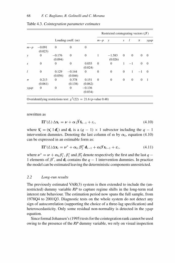
Table 4.3. Cointegration parameter estimates
Restricted cointegrating vectors (β′)
Loading coeff. (α) m−p y s l π ygap
m−p −0.091 0 0 0(0.023)
y 0 −0.176 0 0 1 −1.583 0 0 0 0(0.094) (0.026)
s 0 0 0 0.055 0 0 1 −1 0 0(0.024)
l 0 0.129 −0.144 0 0 0 0 1 −1 0(0.056) (0.046)
π 0.213 0 0.378 0.151 0 0 0 0 0 1(0.061) (0.138) (0.062)
ygap 0 0 0 −0.136(0.034)
Overidentifying restrictions test: χ2(22) = 21.6 (p-value 0.48)
rewritten as
Π∗(L) �xt = ν + α β′xt−1 + εt , (4.10)
where x′t = (x′
t 1 d′t ) and dt is a (q − 1) × 1 subvector including the q − 1
intervention dummies. Denoting the last column of α by αk, equation (4.10)can be expressed in an estimable form as:
Π∗(L)�xt = ν∗ + αk β∗′2 dt−1 + αβ′xt−1 + εt , (4.11)
where ν∗ = ν + αkβ∗1 , β∗
1 and β∗2 denote respectively the first and the last q −
1 elements of β*, and dt contains the q − 1 intervention dummies. In practicethe model can be estimated leaving the deterministic components unrestricted.
2.2 Long-run results
The previously estimated VAR(3) system is then extended to include the (un-restricted) dummy variable RP to capture regime shifts in the long-term realinterest rate behaviour. The estimation period now spans the full sample, from1978Q4 to 2001Q3. Diagnostic tests on the whole system do not detect anysign of autocorrelation (supporting the choice of a three-lag specification) andheteroscedasticity. Only some residual non-normality is detected in the ygapequation.
Since formal Johansen’s (1995) tests for the cointegration rank cannot be usedowing to the presence of the RP dummy variable, we rely on visual inspection
Inflation modelling in the euro area 69
1980 1985 1990 1995 2000
−.025
0
.025
.05First cointegrating vector (normalised on m − p)
1980 1985 1990 1995 2000
−.01
0
.01
Second cointegrating vector (normalised on s)
1980 1985 1990 1995 2000
−.01
0
.01
Third cointegrating vector (normalised on l )
1980 1985 1990 1995 2000
−.025
0
.025
Fourth cointegrating vector (normalised on ygap)
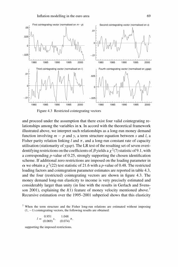
Figure 4.3 Restricted cointegrating vectors
and proceed under the assumption that there exist four valid cointegrating re-lationships among the variables in x. In accord with the theoretical frameworkillustrated above, we interpret such relationships as a long-run money demandfunction involving m − p and y, a term structure equation between s and l, aFisher parity relation linking l and π , and a long-run constant rate of capacityutilisation (stationarity of ygap). The LR test of the resulting set of seven overi-dentifying restrictions on the coefficients ofβ yields a χ2(7) statistic of 9.1, witha corresponding p-value of 0.25, strongly supporting the chosen identificationscheme. If additional zero restrictions are imposed on the loading parameter inα we obtain a χ2(22) test statistic of 21.6 with a p-value of 0.48. The restrictedloading factors and cointegration parameter estimates are reported in table 4.3,and the four (restricted) cointegrating vectors are shown in figure 4.3. Themoney demand long-run elasticity to income is very precisely estimated andconsiderably larger than unity (in line with the results in Gerlach and Svens-son 2001), explaining the I(1) feature of money velocity mentioned above.7
Recursive estimation over the 1995–2001 subperiod shows that this elasticity
7 When the term structure and the Fisher long-run relations are estimated without imposing(1, −1) cointegrating vectors, the following results are obtained:
l = 0.951
(0.069)s,
1.048
(0.074)π,
supporting the imposed restrictions.
70 F. C. Bagliano, R. Golinelli and C. Morana
is remarkably stable over time. The estimated loading parameters show thatpositive deviations from the equilibrium relation between m − p and y cause astrong upward pressure on inflation and output and an error-correcting reactionof real money balances. An increase of the short-term interest rate relative to thelong rate determines a negative reaction of output and an equilibrating responseof the long-term rate. The long-term interest rate exhibits error-correcting be-haviour also in response to positive deviations from the Fisher parity relationwith the inflation rate. Finally, increases in the capacity utilisation rate have apositive impact on inflation (a ‘Phillips curve’) and on the short-term interestrate (a ‘Taylor rule’ effect). The whole set of overidentifying restrictions on theloading factors and the cointegrating vector parameters is never rejected at the5% significance level when the system is estimated recursively from 1995.
3 Permanent and transitory components of inflation
The long-run (cointegration) properties of the data analysed in the previous sec-tion may then be used to disentangle the short- and long-run (‘core’) componentsof the variables analysed, as shown by Stock and Watson (1988) and Gonzaloand Granger (1995). To this aim, we apply the common trends methodologyof King et al. (1991) and Mellander, Vredin and Warne (1992) to our small-scale macroeconomic system and focus in particular on the inflation rate. Inthis context, core inflation is interpreted as the long-run forecast of the inflationrate conditional on the information contained in the variables of the systemand consistent with the long-run cointegration properties of the data. A similardefinition of core inflation is adopted by Cogley and Sargent (2001) in theiranalysis of the dynamic behaviour of post-war US inflation. Moreover, in amultivariate system, structural shocks are likely to be identified more preciselythan, for example, in the bivariate approach of Quah and Vahey (1995), and theforecast error variance decomposition can yield meaningful information aboutthe dynamic effects of different disturbances on the inflation process. The restof this section outlines and applies this econometric methodology to euro-areadata.
3.1 Econometric methodology
As in Mellander, Vredin and Warne (1992) and Warne (1993), the cointegratedVAR in (4.11) can be inverted to yield the following stationary Wold represen-tation for �xt (henceforth, deterministic terms, including the constant vector ν∗
and the dummy variable vector d capturing different real interest rate regimesare omitted for ease of exposition):
�xt = C(L) εt , (4.12)
Inflation modelling in the euro area 71
where C(L) = I + C1L + C2L2 + . . . with∑∞
j=0 j | C j |< ∞. From the rep-resentation in (4.12) the following expression for the levels of the variables canbe derived by recursive substitution:
xt = x0 + C(1)t−1∑j=0
εt− j + C∗(L)εt , (4.13)
where C∗(L) = ∑∞j=0 C∗
j L j with C∗j = − ∑∞
i= j+1 Ci . C(1) captures the long-run effect of the reduced form disturbances in ε on the variables in x and x0 isthe initial observation in the sample.
In order to obtain an economically meaningful interpretation of the dynamicsof the variables of interest from the reduced form representations in (4.12) and(4.13), the vector of reduced form disturbances ε must be transformed into avector of underlying, ‘structural’ shocks, some with permanent effects on thelevel of x and some with only transitory effects. Let us denote this vector ofi.i.d. structural disturbances as ϕt ≡ (ψt
ν t
), where ψ and ν are subvectors of
n − k and k elements, respectively. The structural form for the first differenceof xt is:
�xt = Γ(L)ϕt (4.14)
where Γ(L) = Γ0 + Γ1L + . . . . Since the first element of C(L) in (4.12) is I,equating the first term of the right-hand sides of (4.12) and (4.14) yields thefollowing relationship between the reduced form and the structural shocks:
εt = Γ0ϕt , (4.15)
where Γ0 is an invertible matrix. Hence, comparison of (4.14) and (4.12) showsthat
C(L)Γ0 = Γ(L),
implying that Ci Γ0 = Γi (∀i > 0 ) and C(1)Γ0 = Γ(1). In order to identify theelements of ψt as the permanent shocks and the elements of ν t as the transitorydisturbances, the following restriction on the long-run matrix Γ(1) must beimposed:
Γ(1) = (Γg 0), (4.16)
with Γg an n × (n − k) submatrix. The disturbances in ψt are then allowedto have long-run effects on (at least some of) the variables in xt, whereas theshocks in ν t are restricted to have only transitory effects.
From (4.14) the structural form representation for the endogenous variablesin levels is derived as
xt = x0 + Γ(1)t−1∑j=0
ϕt− j + Γ∗(L)ϕt = x0 + Γg
t−1∑j=0
ψt− j+Γ∗(L)ϕt , (4.17)
72 F. C. Bagliano, R. Golinelli and C. Morana
where the partition of φ and the restriction in (4.16) have been used and Γ*(L)is defined analogously to C*(L) in (4.13). The permanent part in (4.17),
∑t−1j=0
ψt−j, may be expressed as an (n − k)-vector random walk τ with innovationsψ:
τ t = τ t−1 + ψt = τ 0 +t−1∑j=0
ψt− j . (4.18)
Using (4.18) in (4.17), we finally obtain the common trend representation ofStock and Watson (1988) for xt:
xt = x0 + Γgτ t︸ ︷︷ ︸ +Γ∗(L)ϕt︸ ︷︷ ︸ (4.19)
⇒ xt = xct + xnc
t ,
where xct and xnc
t correspond to the ‘trend’ and ‘cycle’ components in theBeveridge–Nelson–Stock–Watson decomposition of xt. According to (4.19) thetrend behaviour of the variables is determined by the permanent disturbancesonly, whereas the cyclical component is determined by all innovations in thesystem, both permanent and transitory. This implies that permanent innovationsalso induce transitory dynamics.
As shown in detail by Stock and Watson (1988), King et al. (1991) and Warne(1993), the identification of separate permanent shocks requires a sufficientnumber of restrictions on the long-run impact matrix Γg in (4.19). Part ofthese restrictions are provided by the cointegrating relations and the consistentestimation of C(1); additional ones are suggested by economic theory (e.g.long-run neutrality assumptions). Finally, having estimated Γg, the behaviourof the variables in xt due to the permanent disturbances only, interpreted asthe long-run forecast of xt, may be computed as x0 + Γgτ t. Formally, such along-run forecast can be expressed as
limh→∞
Et xt+h = x0 + Γgτ t , (4.20)
capturing the values to which the series are expected to converge once theeffect of the transitory shocks have died out (Cogley and Sargent 2001). More-over, from the moving average representation in (4.14), impulse responses andforecast error variance decompositions may be calculated to gauge the relativeimportance of permanent and transitory innovations in determining fluctuationsof the endogenous variables.
3.2 Results
In our common trends framework, the existence of four cointegrating vectorsin the six-variable system implies the presence of two sources of shocks having
Inflation modelling in the euro area 73
permanent effects on at least some of the variables in x′ (m − p, y, s, l, π andygap). As previously mentioned, the four (restricted) cointegrating vectors pro-vide a set of restrictions that can be used to identify the elements of Γg in (4.19).However, one additional restriction is needed to achieve identification. To thisaim, we make the following assumption on the nature of the two permanentshocks in the system: we consider a real shock (ψ r) and a nominal disturbance(ψn). The permanent part (4.18) of the common trends representation is thengiven by the following bivariate random walk:(
τr
τn
)t
=(
µr
µn
)+
(τr
τn
)t−1
+(
ψr
ψn
)t
, (4.21)
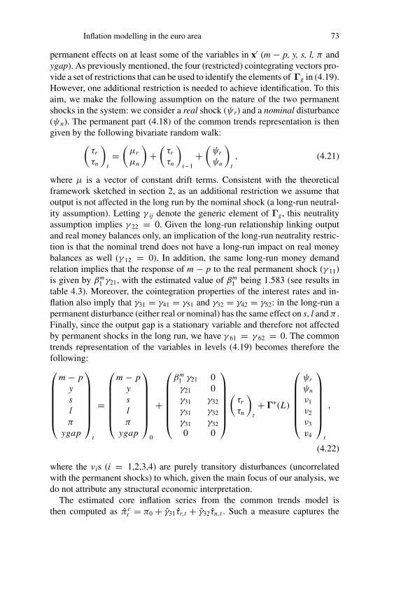
where µ is a vector of constant drift terms. Consistent with the theoreticalframework sketched in section 2, as an additional restriction we assume thatoutput is not affected in the long run by the nominal shock (a long-run neutral-ity assumption). Letting γ ij denote the generic element of Γg, this neutralityassumption implies γ 22 = 0. Given the long-run relationship linking outputand real money balances only, an implication of the long-run neutrality restric-tion is that the nominal trend does not have a long-run impact on real moneybalances as well (γ 12 = 0). In addition, the same long-run money demandrelation implies that the response of m − p to the real permanent shock (γ 11)is given by βm
1 γ21, with the estimated value of βm1 being 1.583 (see results in
table 4.3). Moreover, the cointegration properties of the interest rates and in-flation also imply that γ31 = γ41 = γ51 and γ32 = γ42 = γ52: in the long-run apermanent disturbance (either real or nominal) has the same effect on s, l and π .Finally, since the output gap is a stationary variable and therefore not affectedby permanent shocks in the long run, we have γ 61 = γ 62 = 0. The commontrends representation of the variables in levels (4.19) becomes therefore thefollowing:
m − pyslπ
ygap
t
=
m − pyslπ
ygap
0
+
βm1 γ21 0γ21 0γ31 γ32
γ31 γ32
γ31 γ32
0 0
(τr
τn
)t
+ Γ∗(L)
ψr
ψn
ν1
ν2
ν3
v4
t
,
(4.22)
where the ν is (i = 1,2,3,4) are purely transitory disturbances (uncorrelatedwith the permanent shocks) to which, given the main focus of our analysis, wedo not attribute any structural economic interpretation.
The estimated core inflation series from the common trends model isthen computed as π c
t = π0 + γ31τr,t + γ32τn,t . Such a measure captures the
74 F. C. Bagliano, R. Golinelli and C. Morana
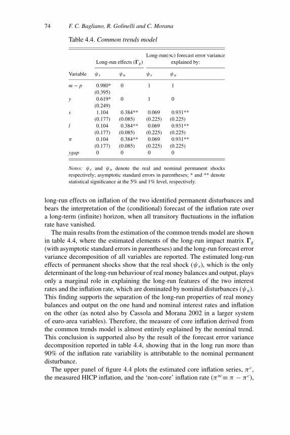
Table 4.4. Common trends model
Long-run(∞) forecast error varianceLong-run effects (Γg) explained by:
Variable ψ r ψn ψ r ψn
m − p 0.980* 0 1 1(0.395)
y 0.619* 0 1 0(0.249)
s 1.104 0.384** 0.069 0.931**(0.177) (0.085) (0.225) (0.225)
l 0.104 0.384** 0.069 0.931**(0.177) (0.085) (0.225) (0.225)
π 0.104 0.384** 0.069 0.931**(0.177) (0.085) (0.225) (0.225)
ygap 0 0 0 0
Notes: ψ r and ψn denote the real and nominal permanent shocksrespectively; asymptotic standard errors in parentheses; * and ** denotestatistical significance at the 5% and 1% level, respectively.
long-run effects on inflation of the two identified permanent disturbances andbears the interpretation of the (conditional) forecast of the inflation rate overa long-term (infinite) horizon, when all transitory fluctuations in the inflationrate have vanished.
The main results from the estimation of the common trends model are shownin table 4.4, where the estimated elements of the long-run impact matrix Γg
(with asymptotic standard errors in parentheses) and the long-run forecast errorvariance decomposition of all variables are reported. The estimated long-runeffects of permanent shocks show that the real shock (ψ r), which is the onlydeterminant of the long-run behaviour of real money balances and output, playsonly a marginal role in explaining the long-run features of the two interestrates and the inflation rate, which are dominated by nominal disturbances (ψn).This finding supports the separation of the long-run properties of real moneybalances and output on the one hand and nominal interest rates and inflationon the other (as noted also by Cassola and Morana 2002 in a larger systemof euro-area variables). Therefore, the measure of core inflation derived fromthe common trends model is almost entirely explained by the nominal trend.This conclusion is supported also by the result of the forecast error variancedecomposition reported in table 4.4, showing that in the long run more than90% of the inflation rate variability is attributable to the nominal permanentdisturbance.
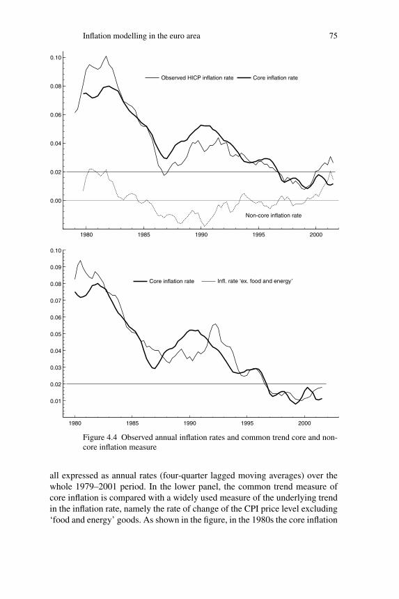
The upper panel of figure 4.4 plots the estimated core inflation series, π c,the measured HICP inflation, and the ‘non-core’ inflation rate (πnc≡ π − π c),
Inflation modelling in the euro area 75
1980 1985 1990 1995 2000
0.00
0.02
0.04
0.06
0.08
0.10
Non-core inflation rate
Observed HICP inflation rate Core inflation rate
1980 1985 1990 1995 2000
0.01
0.02
0.03
0.04
0.05
0.06
0.07
0.08
0.09
0.10
Core inflation rate Infl. rate ‘ex. food and energy’
Figure 4.4 Observed annual inflation rates and common trend core and non-core inflation measure
all expressed as annual rates (four-quarter lagged moving averages) over thewhole 1979–2001 period. In the lower panel, the common trend measure ofcore inflation is compared with a widely used measure of the underlying trendin the inflation rate, namely the rate of change of the CPI price level excluding‘food and energy’ goods. As shown in the figure, in the 1980s the core inflation
76 F. C. Bagliano, R. Golinelli and C. Morana
rate shows more limited fluctuations, ranging from 3% to 8%, with respect toboth observed inflation measures, which vary widely between 2% and 10%. Inparticular, core inflation displays a lower peak during the oil-shock episode ofthe early 1980s (around 8% against 9–10% observed inflation rate), whereas thispattern is reversed during the counter-shock in the mid-1980s. Starting in theearly 1990s, the various inflation rates show more similar behaviour, thoughwith some notable exceptions, namely in 1991, when the core rate began todecrease rapidly in the face of broadly stable (HICP) or increasing (‘ex foodand energy’) actual inflation. Then, all inflation measures declined below the2% level at around the same time in the second half of 1996.
Of particular interest is the relative behaviour of the actual and core inflationseries since the introduction of the euro in January 1999. Initially, the coreand the HICP rates increased from around 1% in early 1999 up to around 2%in mid-2000 (in 2000Q2 the core inflation rate was at 1.8% and the HICPrate at 2.1%). Such an increase is commonly attributed to the sharp rise in oilprices, since the consumer price inflation rate ‘excluding food and energy items’remained stable within a 1–1.2% range. However, the forward-looking, commontrends measure of core inflation signals that the long-run inflation forecast asof 2000Q2 was very close to the HICP observed inflation, even though the ‘exfood and energy’ index showed a lower and stable inflation rate. This evidencecan lend some support to the prudent monetary policy attitude of the ECB in1999 and 2000 in the management of policy interest rates. From 2000Q3, thebehaviour of the estimated core inflation rate started to diverge from that of thetwo observed rates. While the HICP continued to increase up to 3.1% in 2001Q2before going back to 2.6% in the following quarter, and the CPI ‘ex food andenergy’ rate reached 1.8% in 2001Q3, the core inflation rate declined duing thesecond half of 2000 and stabilised at 1.1% in 2001. The increase in inflationobserved in 2001 does not, then, necessarily signal higher long-term inflationprospects.
To give reliable information for policy use, a core inflation measure mustpossess some desirable properties, as stressed by Bryan and Cecchetti (1994)and Wynne (1999). First, the estimated core inflation series should display lowervariability and higher persistence than actual inflation. As noted above, the com-mon trends measure of core inflation portrayed in figure 4.4 is less volatile thanmeasured consumer price inflation. The smoothing property of the estimatedcore inflation is further illustrated in panel A of table 4.5, which reports cor-relation coefficients among changes in the quarterly and annual (four-quartermoving average) inflation rates, including observed inflation and the commontrends core and non-core measures, denoted by �π c and �πnc respectively,with �π ≡ �π c + �πnc. Standard deviations in percentage points are shownon the diagonal. These latter statistics show that there is a remarkable differ-ence in variability between the core and the non-core component: standard
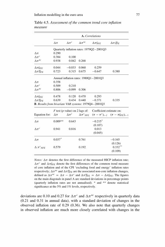
Inflation modelling in the euro area 77
Table 4.5. Assessment of the common trend core inflationmeasure
A. Correlations
�π �π c �πnc �π cNFE �πNFE
nc
Quarterly inflation rates: 1979Q2−2001Q3�π 0.290�π c 0.384 0.100�πnc 0.938 0.042 0.268
�π cNFE 0.044 −0.033 0.060 0.259
�πncNFE 0.723 0.315 0.675 −0.647 0.380
Annual inflation rates: 1980Q1−2001Q3�π 0.358�π c 0.509 0.210�πnc 0.806 −0.099 0.306
�π cNFE 0.478 0.120 0.470 0.293
�πncNFE 0.639 0.434 0.440 −0.371 0.335
B. Results from bivariate VAR systems: 1979Q4−2001Q3
F test (p-value) on 2 lags of: Coefficient estimate on:Equation for: �π �π c �π c
NFE (π − π c)t−1 (π − π cNFE)t−1
�π 0.009** 0.643 −0.215*
(0.107)�π c 0.941 0.816 0.013
(0.045)
�π 0.037* 0.761 −0.165(0.126)
� π cNFE 0.579 0.192 0.332**
(0.109)
Notes: �π denotes the first difference of the measured HICP inflation rate;�π c and �π c
NFE denote the first differences of the common trend measureof core inflation and of the CPI ‘excluding food and energy’ inflation ratesrespectively; �πnc and �πnc
NFE are the associated non-core inflation changes,defined as �πnc = �π − �π c and �πnc
NFE = �π − �π cNFE. The figures
on the main diagonals in panel A are standard deviations in percentage points(quarterly inflation rates are not annualised). * and ** denote statisticalsignificance at the 5% and 1% levels, respectively.
deviations are 0.10 and 0.27 for �π c and �πnc respectively in quarterly data(0.21 and 0.31 in annual data), with a standard deviation of changes in theobserved inflation rate of 0.29 (0.36). We also note that quarterly changesin observed inflation are much more closely correlated with changes in the
78 F. C. Bagliano, R. Golinelli and C. Morana
non-core component (the correlation coefficient is 0.94) than with changes inthe estimated core rate (0.38), and that there is a very low correlation betweencore and non-core inflation changes (0.04 in quarterly and −0.10 in annualdata).
Panel A of Table 4.5 also reports standard deviations and correlations of thechange in the CPI inflation rate ‘excluding food and energy’ goods, �πN F E
(the associated transitory inflation component is denoted by �πncN F E ≡ �π −
�π cN F E ). The standard deviations of changes in both inflation components
obtained from the ex-food and energy price level are large (0.26 for �π cN F E
and 0.38 for �πncN F E in quarterly data), suggesting that this inflation indicator
does not possess the smoothing property displayed by the common trends coreinflation measure.
A second desirable property of a core inflation measure is the ability toforecast future headline inflation rates. The long-run forecasting power of ourcommon trends measure is warranted, since it is estimated as the long-runconditional forecast of inflation. This property can be formally assessed bymeans of a bivariate VAR system including the observed inflation rate and coreinflation π c. As argued by Freeman (1998), the integration and cointegrationproperties of the inflation series require an error-correction representation toperform appropriate Granger-causality tests. In fact, both π and π c are non-stationary, I(1) series, whereas the associated non-core component πnc displaysstationarity, which may be interpreted as evidence of cointegration between thecore inflation measure and the actual inflation rate, since πnc≡ π − π c. Thespecification of the bivariate system is then the following:
�πt = δ10 +2∑
i=1
δ11(i)�πt−i +2∑
i=1
δ12(i)�π ct−i + ρπ (π − π c)t−1 + u1t
�π ct = δ20 +
2∑i=1
δ21(i)�πt−i +2∑
i=1
δ22(i)�π ct−i + ρc(π − π c)t−1 + u2t ,
(4.23)
where two lags are sufficient to eliminate residual serial correlation. Panel B oftable 4.5 reports the results of the F-tests on each block of lagged regressors andthe coefficient estimates of the error-correction coefficients ρπ and ρc. Althoughlags of �π c do not have additional predictive power for the actual inflationrate, a sizeable and significant error-correction coefficient ρπ (−0.22) is esti-mated, showing a tendency of actual inflation to adjust to the core component,whereas no adjustment is detected in the behaviour of π c. We also estimated thebivariate system in (4.23) with π c
N F E in the place of π c. The ex-food and en-ergy inflation measure does not show any strong additional predictive powerfor the observed inflation rate. Moreover, the positive and strongly significant

Inflation modelling in the euro area 79
estimated error-correction coefficient on (π − π cN F E )t−1 suggests that past val-
ues of the inflation rate above the ‘underlying’ component measured by π cN F E
cause an increase in π cN F E itself, reflecting the transmission of transitory shocks
to the permanent component of inflation and casting some doubts on the use-fulness of this measure as an indicator of the long-run inflation trend.
4 A closer look at the properties of inflation components
The common trends model applied in the preceding section decomposes ob-served inflation into a long-run, core component and a transitory, non-core ele-ment. In this section we analyse several features of this decomposition, startingfrom the sources of temporary fluctuations in the inflation rate captured by thenon-core component. Then, we investigate how long it takes for the inflation rateto converge to the core inflation rate, interpreted as a long-run inflation forecast.Finally, we compare the estimated core inflation rate with the inflation forecastat various horizons obtained from a structural dynamic model encompassingthe VAR.
4.1 The nature of the cyclical inflation component
By construction, the common trends core inflation measure embeds only theinformation contained in the permanent shocks hitting the system, abstractingfrom the more volatile dynamics generated by transitory shocks. However,the latter disturbances may not be the only sources of inflation fluctuationsaround the core component. In fact, an important property of the Beveridge–Nelson–Stock–Watson decomposition is that the ‘cyclical’ (here interpretedas the ‘non-core’) component πnc is explained not only by transitory shocks,but also by permanent shocks. Proietti (1997) has proposed a methodology todisentangle in cyclical fluctuations the contribution of permanent shocks fromthe effect of transitory disturbances. Following Cassola and Morana (2002), asimilar decomposition of the cycles can be obtained by rewriting the vector ofcyclical components xnc as
xnct = Γ∗(L)ϕt = Γ∗
1(L)ψt + Γ∗2(L)υt . (4.24)
The vector Γ∗1 (L)ψt gives the contribution of permanent innovations to the
overall cycle (henceforth referred to as the ‘dynamics along the attractor’,DAA), while the vector Γ∗
2 (L)v t measures the contribution of the transitoryinnovations to the overall cycle (‘dynamics towards the attractor’, DTA).
The latter kind of short-run dynamics have the error-correction process asgenerator and, therefore, are disequilibrium fluctuations, while the dynam-ics along the attractor may be related to the overshooting of the variables
80 F. C. Bagliano, R. Golinelli and C. Morana
1985 1990 1995 2000
−.02
−.01
0
.01
.02
.03DTA cycle
1985 1990 1995 2000
−.02
−.01
0
.01
.02 DAA cycle
Figure 4.5 Non-core quarterly inflation rate 1984Q1−2001Q3Note: The quarterly non-core inflation rate is decomposed into ‘dynamicstowards the attractor’ (DTA) and the ‘dynamics along the attarctor’ (DAA)components.
to permanent innovations, i.e. they are the transitional dynamics which takeplace following a shock to the common trend. Since along the attractor thecointegration relationships are satisfied, the DAA adjustment captures equilib-rium fluctuations. This distinction is of particular interest here since it allowsus to attribute deviations of observed inflation from its core rate to the ef-fects of transitory shocks and to the overshooting of the system to permanentshocks.
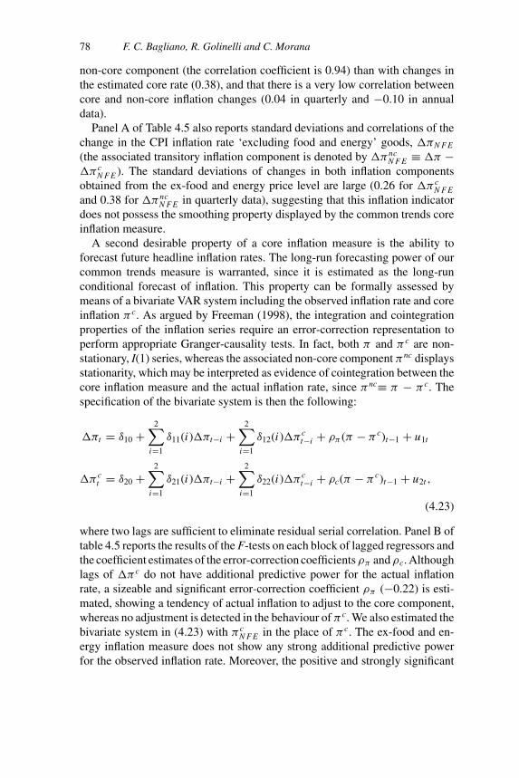
The decomposition of the non-core quarterly inflation rate into the DTAand DAA components is plotted in figure 4.5. After some experimentation weconcluded that twenty lags are sufficient to reconstruct the cyclical components,so that our analysis focuses on the period starting in 1984Q1. As shown in thefigure, both cyclical components are important determinants of the short-runinflation dynamics, with the DTA capturing most of the fluctuations. Over thereconstruction period the DTA explain about 50% of the unconditional varianceof non-core inflation, while the contribution of the DAA is 38%.8 Of the latterproportion, 49% is explained by the real permanent shock ψ r and 32% by thenominal permanent disturbance ψn.
8 The fractions of variance need not to sum to one, since the orthogonality of structural shocksholds only on the entire estimation period, 1978Q1−2001Q3.

Inflation modelling in the euro area 81
4.2 Convergence to the core inflation rate
Our proposed measure of core inflation bears the interpretation of long-runinflation forecast, i.e. π c
t = limh→∞Etπ t+h. Although a long-run perspectiveis consistent with the monetary policymakers’ ability to influence the pricelevel, an infinite horizon is not literally appropriate for the purposes of policyanalysis; for example, the ECB price stability objective is explicitly referredto as a ‘medium-term’ horizon. Then, for the common trend measure of coreinflation to provide useful information to policymakers on the consistency ofcurrent inflation developments with their longer-term price stability goal, it isimportant to assess how long it takes for transitory and permanent shocks toexhaust their effects on the non-core inflation component πnc, i.e. how long ittakes for the observed inflation rate π to converge to the long-run forecast π c.
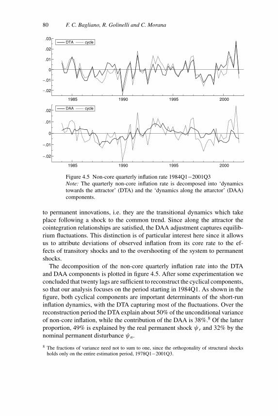
In order to provide some empirical evidence on this issue, we estimated theimpulse response functions of the non-core inflation rate to the various structuraldisturbances. Figure 4.6 shows the impulse responses of the non-core inflationrate to the real and nominal permanent shocks, to a composite permanent shock,i.e. the sum of the two permanent shocks, capturing the ‘dynamics along theattractor’, and to a composite transitory shock, i.e. the sum of the four transitoryshocks, capturing the ‘dynamics towards the attractor’.
As shown in the figure, both composite disturbances have short-lived effectson non-core inflation; in particular, transitory shocks tend to be inflationarywhereas permanent disturbances tend to be deflationary, and complete conver-gence to the reference value is achieved within six and twenty quarters for theDTA shock and the DAA shock, respectively (consistent with the result of thedecomposition of the overall short-run inflation fluctuations in the previous sub-section). As far as the DAA composite disturbance is concerned, the responseof non-core inflation is dominated by the reaction to the real permanent shock,with inflation falling as productivity increases. According to the estimated sig-nificance bands (one standard error), the responses of πnc are not statisticallydifferent from zero after only a few quarters (one and six quarters for DTA andDAA shocks, respectively), suggesting that the overall inflation rate quicklyreverts to its long-run, core component. The empirical evidence therefore sup-ports the proposed core inflation measure as a potentially useful indicator oflong-run inflation prospects over a horizon appropriate for monetary policyevaluation.
4.3 Forecasting inflation from a structural dynamic model
Finally, we compare the estimated core inflation from the common trends modelwith the forecast of a structural econometric model (SEM) derived from thecointegrated VAR system previously estimated. Starting from the cointegrated
82 F. C. Bagliano, R. Golinelli and C. Morana
−.25
0
.25
.5
.75 -SE DTA+SE
-.4
-.2
0
-SE DAA+SE
0 10 20 30 40 0 10 20 30 40
0 10 20 30 40 0 10 20 30 40
−.4
−.2
0
-SE RPS+SE
-.3
-.2
-.1
0
.1
-SE NPS+SE
Figure 4.6 Responses of the non-core quarterly inflation rate to shocks.Note: The upper panels show the impulse response functions of the non-corequarterly inflation rate πnc to composite transitory shocks (DTA), and to com-posite permanent shocks (DAA). The lower panels show the impulse responsefunctions of πnc to the real permanent shock ψ r (RPS), and to the nominalpermanent disturbance ψn (NPS). One-standard error confidence bands havebeen computed by Monte Carlo simulations, with 1000 replications.
VAR set up in section 2.2, we followed a ‘general-to-specific’ modelling strat-egy (Hendry and Mizon, 1993). Zero restrictions were imposed in successivesteps on several lags of the endogenous variables in the six equations of thesystem; after each step a test of the overidentifying restrictions was performed,supporting the restrictions imposed. The FIML estimates of the final specifi-cation of the SEM are shown in table 4.6, where deterministic terms are notreported for brevity.
The system diagnostic tests show the data congruence of the SEM and re-cursive one-step and break-point Chow tests support parameter stability. Thetracking of the model is good (the residual standard errors are relatively small)and the test of the whole set of overidentifying restrictions has a p-value of 0.96(beside the zero restrictions, one additional parameter restriction is imposedin the �y equation, with a p-value of 0.53). Moreover, the residual correlationmatrix shows low coefficients (usually lower than 0.3), suggesting the successof the modelling strategy. Finally, the static long-run real interest rate estimatesreported in the bottom part of table 4.6. are consistent with both the Markov-switching results in section 2.2 and with those in Gerlach and Schnabel (2000).
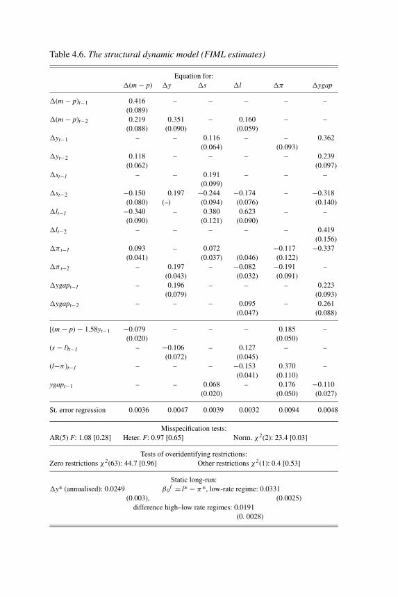
Table 4.6. The structural dynamic model (FIML estimates)
Equation for:�(m − p) �y �s �l �π �ygap
�(m − p)t−1 0.416 – – – – –(0.089)
�(m − p)t−2 0.219 0.351 – 0.160 – –(0.088) (0.090) (0.059)
�yt−1 – – 0.116 – – 0.362(0.064) (0.093)
�yt−2 0.118 – – – – 0.239(0.062) (0.097)
�st−1 – – 0.191 – – –(0.099)
�st−2 −0.150 0.197 −0.244 −0.174 – −0.318(0.080) (–) (0.094) (0.076) (0.140)
�lt−1 −0.340 – 0.380 0.623 – –(0.090) (0.121) (0.090)
�lt−2 – – – – – 0.419(0.156)
�π t−1 0.093 – 0.072 −0.117 −0.337(0.041) (0.037) (0.046) (0.122)
�π t−2 – 0.197 – −0.082 −0.191 –(0.043) (0.032) (0.091)
�ygapt−1 – 0.196 – – – 0.223(0.079) (0.093)
�ygapt−2 – – – 0.095 – 0.261(0.047) (0.088)
[(m − p) − 1.58yt−1 −0.079 – – – 0.185 –(0.020) (0.050)
(s − l)t−1 – −0.106 – 0.127 – –(0.072) (0.045)
(l−π )t−1 – – – −0.153 0.370 –(0.041) (0.110)
ygapt−1 – – 0.068 – 0.176 −0.110(0.020) (0.050) (0.027)
St. error regression 0.0036 0.0047 0.0039 0.0032 0.0094 0.0048
Misspecification tests:AR(5) F: 1.08 [0.28] Heter. F: 0.97 [0.65] Norm. χ2(2): 23.4 [0.03]
Tests of overidentifying restrictions:Zero restrictions χ2(63): 44.7 [0.96] Other restrictions χ2(1): 0.4 [0.53]
Static long-run:�y* (annualised): 0.0249 β0
f = l* − π*, low-rate regime: 0.0331(0.003), (0.0025)
difference high–low rate regimes: 0.0191(0. 0028)

84 F. C. Bagliano, R. Golinelli and C. Morana
1980 1985 1990 1995 2000 2005
0.02
0.04
0.06
0.08
0.10
Core Inflation rate HICP inflation rate
Figure 4.7 Core inflation rate and HICP inflation rate with forecast from amultiple-equation structural dynamic modelNote: One-standard forecast error bands are shown. The shaded area indicatesthe forecast period: 2001Q4−2004Q4.
Turning to the inflation forecasting issue, figure 4.7 displays the annual HICPinflation rate with point forecast values for the period 2001Q4−2004Q4 fromthe estimated SEM. The inflation rate is forecast to decline rapidly from the2.6% level reached in 2001Q3 and stabilise in the 1.7–1.8% range from 2002Q2.Over a two- to three- year horizon these values are broadly consistent with thelong-run inflation forecast measured by the common trends core inflation series,which predicts an annual inflation rate around 1.4%.9
5 Conclusions
A common trends model has been used to estimate the underlying, ‘core’ in-flation behaviour for the euro area from 1978 to 2001. In this framework coreinflation is interpreted as the long-run forecast of inflation conditional on theinformation contained in money growth, output fluctuations and movements ofthe term structure of interest rates.
9 The relatively wide one-standard forecast error bands, computed taking into account the errorvariance only, show that, despite the overall good statistical performance of the econometricmodel, forecasting accuracy is still insufficient to make point inflation forecast from the SEM areliable guide for policymakers.
Inflation modelling in the euro area 85
A price stability-oriented monetary policy has to be forward looking andrespond only to shocks having long-lasting effects on the inflation rate. Thecommon trends core inflation measure may be useful for monetary policy pur-poses since it embodies long-run economic restrictions strongly supported bythe data and bears the interpretation of a long-run forecast, affected only bypermanent disturbances to the inflation rate.
Our empirical exercise on euro-area data shows that purely transitory shockshave short-lived effects on the inflation rate and the estimated core measurecaptures the permanent component of inflation fluctuations over a medium-term horizon consistent with the monetary policy strategy of the EuropeanCentral Bank. An important implication of our results is that deviations of coreinflation, rather than actual inflation, from the price stability objective conveythe appropriate signals for policy action. This conclusion partly contrasts with alarge body of the monetary policy literature, where policy behaviour is modelledby means of a standard Taylor rule.10
As a final word of caution, we observe that a core inflation rate estimatedfrom a common trend model depends on the specification of the system in termsof variables included, sample period, dynamic specification, and other mod-elling choices. However, the core inflation series obtained from the small-scalemacroeconomic model used in this chapter, featuring long-run relationshipsbetween real money balances, output, inflation and interest rates, seems an use-ful benchmark to evaluate the properties of other measures of core inflationcurrently used in the monetary policy debate. As a first step in this direction wecompared the smoothing and forecasting properties of the common trends coreinflation with those of the ‘ex food and energy’ CPI inflation rate. The compar-ison lends support to our core inflation measure as a more reliable indicator ofthe long-run inflation trend.
R E F E R E N C E S
Bagliano, F. C., R. Golinelli and C. Morana, 2002, ‘Core Inflation in the Euro Area’,Applied Economic Letters 9, 353–7.
Bodo, G., R. Golinelli and G. Parigi, 2000, ‘Forecasting Industrial Production in theEuro Area’, Empirical Economics 25(4), 541–61.
Brand, C. and N. Cassola, 2000, ‘A Money Demand System for Euro Area M3’, EuropeanCentral Bank Working Paper no. 39.
Bryan, M. F. and S. G. Cecchetti, 1994, ‘Measuring Core Inflation’, in N. G. Mankiw(ed.), Monetary Policy, Chicago: University of Chicago Press for NBER, pp. 195–215.
10 A first application of a modified monetary policy rule which determines short-term interest ratesaccording to the deviations of core inflation from the price stability objective is provided byCassola and Morana (2002).
86 F. C. Bagliano, R. Golinelli and C. Morana
Cassola, N. and C. Morana, 2002, ‘Monetary Policy and the Stock Market in the EuroArea’, European Central Bank Working Paper no. 119.
Cecchetti, S. G., 1997, ‘Measuring Short-Run Inflation for Central Bankers’, FederalReserve Bank of St. Louis Review 79(3), 143–56.
Coenen, G. and J. L. Vega, 2001, ‘The Demand for M3 in the Euro Area’, Journal ofApplied Econometrics 16(6), 727–48.
Cogley, T., 2002, ‘A Simple Adaptive Measure of Core Inflation’, Journal of Money,Credit and Banking 34(1), 94–113.
Cogley, T. and T. J. Sargent, 2001, ‘Evolving Post-World War II U.S. Inflation Dynam-ics’, in B. S. Bernanke and K. Rogoff (eds.), NBER Macroeconomics Annual 2001,Cambridge, MA: MIT Press, pp. 331–72.
Davies, R. B., 1987, ‘Hypothesis Testing when a Nuisance Parameter is Present OnlyUnder the Alternative’, Biometrika 74, 33–43.
Dedola L., E. Gaiotti and L. Silipo, 2001, ‘Money Demand in the Euro Area: Do NationalDifferences Matter?’, Bank of Italy Discussion Paper no. 405.
Espasa, A., R. Albacete and E. Senra, 2002, ‘Forecasting EMU Inflation: A Disaggre-gated Approach by Countries and Components’, European Journal of Finance 8(4),402–21.
European Central Bank, 1999, ‘The Stability-Oriented Monetary Policy Strategy of theEurosystem’, Monthly Bulletin, January, 39–49.
2000, ‘The Two Pillars of the ECB’s Monetary Policy Strategy’, Monthly Bulletin,November, 37–48.
2001, ‘Framework and Tools of Monetary Analysis’, Monthly Bulletin, May, 41–58.Freeman, D. G., 1998, ‘Do Core Inflation Measures Help Forecast Inflation?’, Economics
Letters 58, 143–7.Galı, J., M. Gertler and J. D. Lopez-Salido, 2001, ‘European Inflation Dynamics’, Eu-
ropean Economic Review 45(7), 1237–70.Gerlach, S. and G. Schnabel, 2000, ‘The Taylor Rule and Interest Rates in the EMU
Area’, Economics Letters 67, 165–71.Gerlach, S. and L. E. O. Svensson, 2001, ‘Money and Inflation in the Euro Area: A
Case of Monetary Indicators?’, Bank for International Settlements Working Paperno. 98, January.
Golinelli, R. and S. Pastorello, 2002, ‘Modelling the Demand for M3 in the Euro Area’,European Journal of Finance 8(4), 371–401.
Gonzalo, J. and C. W. J. Granger, 1995, ‘Estimation of Common Long-Memory Com-ponents in Cointegrated Systems’, Journal of Business and Economic Statistics 13,27–35.
Hallman, J. J., R. D. Porter and D. H. Small, 1991, ‘Is the Price Level Tied to theM2 Monetary Aggregate in the Long Run?’, American Economic Review 81(4),841–58.
Hamilton, J. D., 1989, ‘A New Approach to the Economic Analysis of NonstationaryTime Series and the Business Cycle’, Econometrica 57, 357–84.
Hansen, B. E., 1992, ‘Tests for Parameter Instability in Regressions with I(1) Processes’,Journal of Business and Economics Statistics 10, 321–35.
Hendry, D. F. and G. E. Mizon, 1993, ‘Evaluating Dynamic Econometric Models by En-compassing the VAR’, in P. C. B. Phillips (ed.), Models, Methods and Applicationsof Econometrics, Oxford: Basil Blackwell, pp. 272–300.
Inflation modelling in the euro area 87
Johansen, S., 1995, Likelihood-Based Inference in Cointegrated Vector AutoregressiveModels, Oxford: Oxford University Press.
King, R. J., C. Plosser, J. H. Stock and M. W. Watson, 1991, ‘Stochastic Trends andEconomic Fluctuations’, American Economic Review 81, 819–40.
Marcellino, M., J. H. Stock and M. W. Watson, 2003, ‘Macroeconomic Forecasting in theEuro Area: Country Specific Versus Area-wide Information’, European EconomicReview 47(1), 1–18.
Mellander, E., A. Vredin and A. Warne, 1992, ‘Stochastic Trends and Economic Fluc-tuations in a Small Open Economy’, Journal of Applied Econometrics 7, 369–94.
Ng, S. and P. Perron, 1995, ‘Unit Root Tests in ARIMA Models with Data-DependentMethods for the Selection of the Truncation Lag’, Journal of the American Statis-tical Association 90(429), 268–81.
Perron, P., 1997, ‘Further Evidence on Breaking and Trend Functions in MacroeconomicVariables’, Journal of Econometrics 55, 355–85.
Proietti, T., 1997, ‘Short-Run Dynamics in Cointegrating Systems’, Oxford Bulletin ofEconomics and Statistics 59(3), 403–22.
Quah, D. and S. P. Vahey, 1995, ‘Measuring Core Inflation’, Economic Journal 105,1130–44.
Rudebusch, G. D. and L. E. O. Svensson, 1999, ‘Policy Rules for Inflation Targeting’,in J. B. Taylor (ed.), Monetary Policy Rules, Chicago: University of Chicago Pressfor NBER, pp. 203–46.
2002, ‘Eurosystem Monetary Targeting: Lessons from US Data’, European EconomicReview 46(3), 417–42.
Staiger, D., J. H. Stock and M. W. Watson, 2001, ‘Prices, wages and the US NAIRU inthe 1990s’, NBER Working Paper no. 8320.
Stock, J. H. and M. W. Watson, 1988, ‘Testing for Common Trends’, Journal of theAmerican Statistical Association 83, 1097–107.
Taylor, J. B., 1999, ‘The Robustness and Efficiency of Monetary Policy Rules as Guide-lines for Interest Rate Setting by the European Central Bank’, Journal of MonetaryEconomics 43, 655–79.
Warne, A., 1993, ‘A Common Trends Model: Identification, Estimation and Inference’,IIES, Stockholm University, Seminar Paper no. 555.
Wynne, M. A., 1999, ‘Core Inflation: A Review of Some Conceptual Issues’, EuropeanCentral Bank Working Paper no. 5.


![23.Inflation - pdg.lbl.govpdg.lbl.gov/2017/reviews/rpp2017-rev-inflation.pdf · 23.Inflation 5 models [22,23,24], where inflation inside the bubble has a finite duration, leaving](https://img.pdfslide.us/doc/110x75/5e11caf48b6af83dd22a3107/23iniation-pdglbl-23iniation-5-models-222324-where-iniation-inside.jpg)