Holographic inﬂation Kostas Skenderis - University of Cretehep.physics.uoc.gr/cosmo10/talks/Skenderis.pdf · Holographic inﬂation Kostas Skenderis Institute for Theoretical Physics

IntroductionCosmological observables

ResultsDerivation

Conclusions

Holographic inflation

Kostas Skenderis

Institute for Theoretical Physics andKorteweg-de Vries Institute for Mathematics

University of Amsterdam

Crete Workshop on the Frontiers of CosmologyHeraklion, Greece

April 2, 2010

Kostas Skenderis Holographic inflation


ResultsDerivation

Conclusions

Outline

1 Introduction

2 Cosmological observables

3 Results

4 DerivationCosmological PerturbationsThe domain-wall/cosmology correspondenceHolography: a primerHolography for cosmologyBeyond weak gravitational description

5 Conclusions



ResultsDerivation

Conclusions

Cosmology

Over the last two decades, striking new observations havetransformed cosmology from a qualitative to a quantitativescience:

A minimal set of just six parameters characterizes the observed uni-verse, all of which are now known to within a few percent.

Forthcoming experiments (e.g. the Planck satellite) promise awealth of new precision data.This presents a unique window to Planck-scale physics and achallenge (and an opportunity) for fundamental theory.



ResultsDerivation

Conclusions

The origin of structure

All inhomogeneity in the present day universe may be tracedback to primordial fluctuations in the matter density andcurvature of the early universe.These fluctuations may be imaged directly through observationsof the cosmic microwave background (e.g., using the WMAPsatellite).

A widely accepted explanation for the origin of these fluctuationsis the theory of inflation, which postulates the early universeunderwent a brief period of rapid, accelerated expansion.

Despite its successes, the theory of inflation is still unsatisfactoryin a number of ways (e.g., fine-tuning, initial conditions,trans-Planckian issues).



ResultsDerivation

Conclusions

With future observations promising an unprecedented era of precisioncosmology, the constraints on cosmological parameters are expectedto tighten further still, particularly as regards the inflationary sector.

It thus become imperative that

inflation is embedded in a UV complete theory (indeed there isincreasing amount of effort devoted to embedding inflation instring theory),alternative scenarios are developed.

The holographic approach that we undertake provides both.



ResultsDerivation

Conclusions

Holography

The idea of holography [’t Hooft (1993)] emerged from black holesphysics as an answer to the question:Why is black hole entropy proportional to the area of the horizonrather than the volume the black hole occupies?

Definition

Holography states that a theory which includes gravity can bedescribed by a theory with no gravity is one fewer dimension.

Holography became a prominent research direction whenholographic dualities were found in string theory [Maldacena(1997)], [Gubser, Klebanov, Polyakov (1998)] [Witten (1998)].



ResultsDerivation

Conclusions

Holography

The examples found in string theory involve spacetimes withnegative cosmological constant but the general argument forholography is applicable to any theory of gravity.In particular, it should apply to our own universe.The purpose of this work is to propose a concrete holographicframework applicable to our own universe and in particular to itscosmological evolution.



ResultsDerivation

Conclusions

Holography for cosmology

Specifically, I will address the question:

Can a four-dimensional inflationary cosmology be described in termsof a three-dimensional QFT? (without gravity!)



ResultsDerivation

Conclusions

References

The talk is based onPaul McFadden, KS,Holography for Cosmology,arXiv:0907.5542Paul McFadden, KS,The Holographic Universe,arXiv:1007.2007Adam Bzowski, Paul McFadden, KSon-going



ResultsDerivation

Conclusions

Outline

1 Introduction


3 Results


5 Conclusions



ResultsDerivation

Conclusions

Outline

1 Introduction


3 Results


5 Conclusions



ResultsDerivation

Conclusions

Form of the primordial perturbationsThe primordial scalar power spectrum ∆2

S may be characterized by anamplitude A and a spectral tilt ns according to

∆2S = A (q/q0)

ns−1,

where q is the wavenumber of the perturbations and q0 is an arbitraryscale. The WMAP data then yield (for q0 = 0.002Mpc−1)

A = (2.43± 0.11)× 10−9, ns−1 = −0.037± 0.014,

i.e., the perturbations have small amplitude and are nearly scaleinvariant.

These two small numbers should appear naturally in any theorythat explains the data.



ResultsDerivation

Conclusions

Scalar running

In reality, the spectral tilt ns may be a function of momentum q.This is parametrized by the “running”, αs, where

αs = dns/d ln q.

Observationally

αs = −0.022± 0.020(68%CL)

Data from [Komatsu et al 1001.4538]



ResultsDerivation

Conclusions

Tensor Power spectrum

Tensor power spectrum ∆2T :

∆2T(q) = At(q∗) (q/q∗)

nt(q∗)

Only upper limits on At and nt.Tensor-to-scalar ratio r = Pt/Ps. Observationally,

r < 0.22(95%C.L.)



ResultsDerivation

Conclusions

Non-Gaussianity

While the power spectrum is related to 2-point functions (as wewill review later), non-gausianities are related to higher-pointfunctions, e.g.

〈ζ~q1ζ~q2ζ~q3〉 = (2π)3δ(~q1 +~q2 +~q3)fNLF(q1, q2, q3)

F(q1, q2, q3) is a function of the momenta.Observationally,

fNL = 32± 21(68%CL)



ResultsDerivation

Conclusions

Outline

1 Introduction


3 Results


5 Conclusions



ResultsDerivation

Conclusions

Results

Our two main results are:

Standard inflation is holographic.

There are holographic models that have different phenomenology thanstandard inflation but they are nevertheless consistent with current ob-servations.



ResultsDerivation

Conclusions

Standard inflation is holographic

Assuming that the standard gauge/gravity duality is valid andrestricting to single-scalar models (for simplicity) we give amathematical proof that:

Inflationary cosmological observables, such as the powerspectrum and non-gausianities, of four dimensional inflationarymodels are encoded in correlation functions of strongly coupledthree dimensional QFT.

→ This provides a UV completion for standard inflation: the threedimensional QFTs that enter this discussion are well-definedtheories: they are either conformal or super-renormalizable.



ResultsDerivation

Conclusions

New holographic models

Standard inflation is linked to strongly coupled QFTs. There are newmodels based on weakly coupled QFT.

In these models gravity is strongly coupled at early times.They provide a new mechanism for a scale invariant spectrum.They are compatible with current observations, yet they havedifferent phenomenology than standard inflation.

→ Alternative scenarios to standard inflation.



ResultsDerivation

Conclusions

Smoking-gun for new holographic models

In our holographic models the running is minus the deviationfrom scale invariance (to leading order):

α = −(ns−1)

In conventional slow-roll inflation, however, α/(ns−1) is verysmall (of first order in slow-roll).

⇒ Predictions of new holographic scenario are different fromstandard inflation.



ResultsDerivation

Conclusions

WMAP data Komatsu et al. arXiv:0803.0547.

Solid line:

α = −(ns−1)



ResultsDerivation

Conclusions

The holographic universe



ResultsDerivation

Conclusions

Cosmological PerturbationsThe domain-wall/cosmology correspondenceHolography: a primerHolography for cosmologyBeyond weak gravitational description

Outline

1 Introduction


3 Results


5 Conclusions



ResultsDerivation

Conclusions


Part I: Plan

In the first part we will explain the sense in which inflation isholographic.

Review standard inflationary computations.Review how to compute strong coupling QFT results usingstandard gauge/gravity duality.Show that the inflationary results can be fully expressed in termsof correlators of strongly coupled QFTs.



ResultsDerivation

Conclusions


Cosmological Perturbations

We start by reviewing standard inflationary cosmology.

We will discuss single field (for simplicity) four dimensionalinflationary models,

S =1

2κ2

∫d4x√−g(R− (∂Φ)2 − 2κ2V(Φ))

We assume a spatially flat background (for simplicity) and perturb

ds2 = −dt2 + a2(t)[δij + hij(t,~x)]dxidxj

Φ = ϕ(t) + δϕ(t,~x)

where hij = ψ(z,~x)δij + ∂i∂jχ(z,~x) + γij(z,~x)γij is transverse traceless and we form the gauge invariantcombination ζ = −ψ/2 + (H/ϕ)δϕ.



ResultsDerivation

Conclusions


Cosmological perturbations

The equations for perturbations take the form:

0 = ζ + (3H + ε/ε)ζ + a−2q2ζ

0 = γij + 3Hγij + a−2q2γij

where H is the Hubble function and ε = 2(H′/H)2 is the slow-rollparameter. We are not assuming that ε is small.



ResultsDerivation

Conclusions


Power spectrumIn the inflationary paradigm, cosmological perturbations are assumedto originate at sub-horizon scales as quantum fluctuations.

Quantising the perturbations in the usual manner,

〈ζ(t,~q)ζ(t,−~q)〉 = |ζq(t)|2

〈γij(t,~q)γkl(t,−~q)〉 = 2|γq(t)|2Πijkl,

where Πijkl is the transverse traceless projection operator andζq(t) and γq(t) are the mode functions.The superhorizon power spectra are obtained by

∆2S(q) =

q3

2π2 |ζq(0)|2, ∆2T(q) =

2q3

π2 |γq(0)|2,

where γq(0) and ζq(0) are the constant late-time values of thecosmological mode functions. Initial conditions are set by theBunch-Davies vacuum.



ResultsDerivation

Conclusions


Power spectrum through response functions

In preparation to the holographic discussion, we rewrite the powerspectrum as follows.

We define the response functions as

Πζ = Ωζ, Πγij = Eγij,

where Πζ and Πγij are the canonical momenta.

One can show that

|ζq|−2 = −2Im[Ω(q)], |γq|−2 = −4Im[E(q)].

so the power spectra can be expressed in terms of the late timebehavior of the response functions.



ResultsDerivation

Conclusions


Domain-wall/cosmology correspondence

The springboard for our discussion is a correspondence betweencosmologies and domain-wall spacetimes.

Domain-wall spacetime:

ds2 = dr2 + e2A(r)dxidxi

Φ = Φ(r)

This solves the field equations that follow from

SDW =1

2κ2

∫d4x√

g [−R + (∂Φ)2 + 2κ2V(Φ)],



ResultsDerivation

Conclusions



One can prove the following:

Domain-wall/Cosmology correspondence

For every domain-wall solution of a model with potential V there is aFRW solution for a model with potential (V = −V). [Cvetic, Soleng(1994)], [KS, Townsend (2006)]

The correspondence also applies to open and closed FRWuniverses which correspond to curved domain-walls.The correspondence can be understood as analytic continuationfor the metric. The flip in the sign of V guarantees that the scalarfield remains real.An equivalent way to state the correspondence is

κ2 = −κ2



ResultsDerivation

Conclusions


Domain-walls and holography

Domain-wall spacetimes enter prominently in holography. Theydescribe holographic RG flows.

The AdSd+1 metric is the unique metric whose isometry group isthe same as the conformal group in d dimensions. This is themain reason why the bulk dual of a CFT is AdS.The domain-wall spacetimes are the most general solutionswhose isometry group is the Poincaré group in d dimensions.Thus, if a QFT has a holographic dual the bulk solution must beof the domain-wall type.



ResultsDerivation

Conclusions


Holographic RG flows

There are two different types of domain-wall spacetimes whoseholographic interpretation is fully understood.

1 The domain-wall is asymptotically AdSd+1,

A(r) → r, Φ(r) → 0, as r →∞

This corresponds to a QFT that in the UV approaches a fixedpoint. The fixed point is the CFT which is dual to the AdSspacetime approached as r →∞.



ResultsDerivation

Conclusions


Holographic RG flows

2 The domain-wall has the following asymptotics

A(r) → n log r, Φ(r) →√

2n log r, as r →∞

This case has only been understood recently [Kanitscheider, KS,Taylor (2008)] [Kanitscheider, KS (2009)].

→ Specific cases of such spacetimes are ones obtained by takingthe near-horizon limit of the non-conformal branes (D0, D1, F1,D2, D4).

→ These solutions describe QFTs with a dimensionful couplingconstant in the regime where the dimensionality of the couplingconstant drives the dynamics.



ResultsDerivation

Conclusions



Let us see how the correspondence acts on the domain-wallsdescribing holographic RG flows.

1 Asymptotically AdS domain-walls are mapped to inflationarycosmologies that approach de Sitter spacetime at late times,

ds2 → ds2 = −dt2 + e2tdxidxi, as t →∞

2 The second type of domain-walls is mapped to solutions thatapproach power-law scaling solutions at late times,

ds2 → ds2 = −dt2 + t2ndxidxi, as t →∞



ResultsDerivation

Conclusions


Holography: a primer

The holographic dictionary for cosmology will be based on thestandard holographic dictionary, so we now briefly review standardholography:

1 There is 1-1 correspondence between local gauge invariantoperators O of the boundary QFT and bulk supergravity modesΦ.→ The bulk metric corresponds to the energy momentum tensor of

the boundary theory.→ Bulk scalar fields correspond to boundary scalar operators, i.e.

FµνFµν , ψψ, etc.

2 Correlation functions of gauge invariant operators can beextracted from the asymptotics of bulk solutions.



ResultsDerivation

Conclusions


Asymptotic solutions

To understand the holographic computations we need to know a fewthings about the structure of solutions of Einstein’s theory with anegative cosmological constant.

For the metric, the most general asymptotic form (in 4 bulkdimensions) looks like [Fefferman, Graham (1985)]

ds2 = dr2 + e2rgij(x, r)dxidxj

gij(x, r) = g(0)ij(x) + e−2rg(2)ij(x) + e−3rg(3)ij(x) + ...

g(0)(x) is the metric of the spacetime where the boundary theorylives and (as such) it is also the source of the boundary energymomentum tensor.



ResultsDerivation

Conclusions


Correlation functions

Using the formalism of holographic renormalization, we then finda precise relation between correlation functions and asymptotics[de Haro, Solodukhin, KS (2000)]

〈Tij〉 =3

2κ2 g(3)ij.

Higher-point functions are obtained by differentiating the 1-pointfunctions w.r.t. sources and then setting the sources to theirbackground value

〈Ti1j1(x1)Ti2j2(x2) · · ·Tinjn(xn)〉 ∼δ(n−1)g(3)i1j1(x1)

δg(0)i2j2(x2) · · · δg(0)injn(xn)

∣∣∣g(0)=η

Thus to solve the theory we need to know g(3) as a function ofg(0). This can be obtained perturbatively: 2-point functions areobtained by solving linearized fluctuations, 3-point functions bysolving quadratic fluctuations etc.



ResultsDerivation

Conclusions


Correlation functions

Using the formalism of holographic renormalization, we then finda precise relation between correlation functions and asymptotics[de Haro, Solodukhin, KS (2000)]

〈Tij〉 =3

2κ2 g(3)ij.

Higher-point functions are obtained by differentiating the 1-pointfunctions w.r.t. sources and then setting the sources to theirbackground value

〈Ti1j1(x1)Ti2j2(x2) · · ·Tinjn(xn)〉 ∼δ(n−1)g(3)i1j1(x1)

δg(0)i2j2(x2) · · · δg(0)injn(xn)

∣∣∣g(0)=η

Thus to solve the theory we need to know g(3) as a function ofg(0). This can be obtained perturbatively: 2-point functions areobtained by solving linearized fluctuations, 3-point functions bysolving quadratic fluctuations etc.



ResultsDerivation

Conclusions


Correlation functions for holographic RG flows

To compute 2-point functions we perturb around the domain-wall

ds2 = dr2 + e2A(r)[δij + hij(r, xi)]dxidxj

Φ = ϕ(r) + δϕ(r, xi)

where hij = ψ(r, xi)δij + ∂i∂jχ(r, xi) + γij(r, xi)γij is transverse traceless and we form the gauge invariantcombination ζ = −ψ/2 + (H/ϕ)δϕ and H = −W/2, with W thefake superpotential.



ResultsDerivation

Conclusions



The linearized equations are given by [Bianchi, Freedman, KS(2001)], [Papadimitriou, KS (2004)],

0 = ζ + (3H + ε/ε)ζ−q2e−2Aζ

0 = γij + 3Hγij−q2e−2Aγij,

Comparing with the cosmological perturbations, we find that theequations are mapped to each other provided

q = −iq



ResultsDerivation

Conclusions


Domain-wall/Cosmology correspondence

In other words, we have just establish that:

The Domain-wall/cosmology correspondence maps not only the back-ground solutions but also linear fluctuations around them.

This extends to all orders in fluctuations.



ResultsDerivation

Conclusions



We now want to extract the QFT correlators from the linearizedsolution.

Schematically, we must expand the linearized solution near ther →∞ and extract the piece that scales like e−3r.

It is convenient to work in terms of response functions[Papadimitriou, KS (2004)]

Πζ = −Ωζ, Πγij = −Eγij,

where Πζ , Πγij are radial canonical momenta.



ResultsDerivation

Conclusions


2-point functions for holographic RG flows

The 2-point function of the energy momentum tensor is then given by

〈Tij(q)Tkl(−q)〉 = A(q)Πijkl + B(q)πijπkl,

where

Πijkl =12(πikπlj + πilπkj − πijπkl), πij = δij − qiqj/q2.

A(q) = 4 [E(q)](0)

B(q) =14

[Ω(q)

](0) .

The subscript indicates that one should pick the term with appropriatescaling in the asymptotic expansion.



ResultsDerivation

Conclusions


Holography for cosmologyWe are now ready to show that the power spectrum is holographic.

We have shown earlier that

∆2S(q) =

−q3

4π2ImΩ(0)(q), ∆2

T(q) =−q3

2π2ImE(0)(q),

Applying the analytic continuation,

κ2 = −κ2, q = −iq

we find:

∆2S(q) =

q3

2π2

(−1

8ImB(−iq)

), ∆2

T(q) =2q3

π2

(−1

ImA(−iq)

),

where the holographic 2-point function is




ResultsDerivation

Conclusions


Non-gaussianity [McFadden, KS], [Bzowski, McFadden, KS] to appear

A similar type of analysis shows a direct link between non -Gausianities and holographic higher-point functions. The preciseholographic dictionary requires technical control over a number ofissues. For example, for 3-point functions:

one needs to know the precise form of the cosmologicalperturbations to second order (without slow-roll).one needs to know the general form of

〈Ti1j1(q1)Ti2j2(q2)Ti3j3(q3)〉 = ...

Both of these are near completion ...



ResultsDerivation

Conclusions


Example: power-law cosmology

We have established that any inflationary model is holographic. Letus now see how this works in a simple example.

Consider the potential

V(ϕ) = V0 exp(−√

2/nκϕ)

The corresponding solution is

ds2 = −dt2 + (t/t0)ndxidxi, κϕ =√

2n ln t/t0

When n = 7 this solution is related via the DW/cosmologycorrespondence to the near-horizon limit of a stack of D2 branes.



ResultsDerivation

Conclusions


Example: power-law cosmology

The holographic 2-point functions have been c omputed in[Kanitscheider, KS, Taylor (2008)]

A(q) = 2nB(q) = − 2π4σΓ2(σ) sinπσ

κ−2q2σ.

where σ = (3n− 1)/(n− 1) > 3/2.Using the analytic continuation one obtains

∆2T(q) =

16n

∆2S(q) =

4σΓ2(σ)π3 κ2q3−2σ,

which is the correct answer.



ResultsDerivation

Conclusions


Analytic continuation in QFT variables

The analytic continuation

κ2 = −κ2, q = −iq,

translates in QFT language to

N2 → −N2, q → −iq



ResultsDerivation

Conclusions


The proposal



ResultsDerivation

Conclusions


Pseudo-QFT

We operationally define the pseudo-QFT as follows:

we do the computation in the QFT dual to the domain-wall andthen analytically continue parameters and momentaappropriately.

Perhaps a more fundamental perspective is to consider the QFTaction with complex parameters as the fundamental object.

Then the results on different real domains will be applicable toDW/cosmology as appropriate.

→ The supergravity realization of the DW/cosmologycorrespondence works this way.



ResultsDerivation

Conclusions


Part II: Beyond the weak gravitational description

So far the discussion was on the gravitational side.We inferred a QFT description using known gauge/gravitydualities and analytic continuation, but all computations weredone on the gravitational side.When gravity is strongly coupled the QFT description is weaklycoupled, so one may use the duality.This allows us to compute the late time behavior of the responsefunctions and therefore the power spectra etc when the earlytime behavior is strongly coupled/stringy.



ResultsDerivation

Conclusions


Holographic phenomenology for cosmology

The boundary theory will be a combination of gauge fields,fermions and scalars and it should admit a large N expansion.To extract predictions we need to compute the coefficients A andB,


analytically continue the result and insert in the formulae for thepower spectra.One can then look for a holographic theory that models well theobservations.



ResultsDerivation

Conclusions


Holographic phenomenology for cosmology

As a starting point one can consider the strong coupling versionof asymptotically dS cosmologies and power-law cosmology.In this talk we focus on QFTs dual to the latter. These aresuper-renormalizable QFTs that depend on a single dimensionfulcoupling:

S =1

g2YM

∫d3xtr

[12

FIijF

Iij +12(DφJ)2 +

12(DχK)2 + ψL /DψL

+ λM1M2M3M4ΦM1ΦM2ΦM3ΦM4 + µαβML1L2

ΦMψL1α ψ

L2β

].



ResultsDerivation

Conclusions


A new mechanism for scale invariant spectrum

We need to compute the 2-point function of Tij. The leading ordercomputation is at 1-loop:

The answer follows from general considerations:

The stress energy tensor has dimension 3 in three dimensions.1-loop amplitudes are independent of g2

YM

There is a factor of N2 because of the trace over the gaugeindices.

〈TijTkl〉 ∼ N2q3



ResultsDerivation

Conclusions


A new mechanism for scale invariant spectrum

Recalling the holographic map:

∆2S ∼

q3

〈TT〉∼ 1

N2

Spectrum scale invariant to leading order, independent of thedetails of the holographic theory.

Furthermore,

Amplitude of power spectrum A ∼ 1/N2.Small A ∼ 10−9 ⇒ large N ∼ 104, justifying the large N limit.



ResultsDerivation

Conclusions


Power spectra

The complete answer is

A(q) = CAN2q3 + O(g2YM), B(q) = CBN2q3 + O(g2

YM),

where

CA = (NA +Nφ +Nχ + 2Nψ)/256, CB = (NA +Nφ)/256.

NA : # of gauge fields,Nφ : # of minimally coupled scalars,Nχ : # of conformally coupled scalars,Nψ : # of fermions.

⇒ ∆2S(q) =

116π2N2CB

+ O(g2YM), ∆2

T(q) =2

π2N2CA+ O(g2

YM).



ResultsDerivation

Conclusions


Tensors-to-scalar ratio

It follows thatr = ∆2

T/∆2S = 32CB/CA,

The upper bound on r translates into a constraint on the fieldcontent of the dual QFT.A smaller upper bound on r requires increasing the number ofconformal scalars and massless fermions and/or decreasing thenumber of gauge fields and minimal scalars.



ResultsDerivation

Conclusions


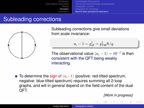
Subleading corrections

Subleading corrections give small deviationsfrom scale invariance:

ns − 1 ∼ g2eff = g2

YMN/q.

The observational value (ns − 1) ∼ 10−2 is thenconsistent with the QFT being weaklyinteracting.

To determine the sign of (ns−1) (positive: red-tilted spectrum,negative: blue-tilted spectrum) requires summing all 2-loopgraphs, and will in general depend on the field content of the dualQFT.

[Work in progress]



ResultsDerivation

Conclusions


2-loop details

Super-renormalizable theories often have infrared problems. Thespecific type of theories we consider however are well-defined: g2

YMacts as an infrared cut-off. [Jackiw, Templeton (1981)] [Appelquist,Pisarski (1981)].The 2-loop integrals are indeed finite and one obtains:

A(q) = CAN2q3[1 + DAg2eff ln(q/q∗) + O(g4

eff)],

B(q) = CBN2q3[1 + DBg2eff ln(q/q∗) + O(g4

eff)],

where g2eff = g2

YMN/q and DA and DB are numerical constants.This leads to

nS(q)−1 = −DBg2eff + O(g4

eff), nT(q) = −DAg2eff + O(g4

eff).



ResultsDerivation

Conclusions


Running

Independent of the details of the theory, the scalar spectral indexruns as

αs =dns

d ln q= −(ns−1) + O(g4

eff).

This prediction is qualitatively different from slow-roll inflation, forwhich αs/(ns−1) is of first-order in slow-roll.



ResultsDerivation

Conclusions


Non-Gaussianity [in progress]

To compute the leading non-Gaussianity one needs to compute

〈Ti1j1(q1)Ti2j2(q2)Ti3j3(q3)〉

Leading contribution is 1-loop and does not depends on theinteractions of the holographic model.Preliminary results show that these holographic models predictfNL ∼ O(100), in agreement with current expectations!



ResultsDerivation

Conclusions

Outline

1 Introduction


3 Results


5 Conclusions



ResultsDerivation

Conclusions

Conclusions

I have presented a holographic description of inflationarycosmology in terms of a 3-dimensional QFT (without gravity!)When gravity is weakly coupled, holography correctly reproducesstandard inflationary predictions for cosmological observables.When gravity is strongly coupled, one finds new models thathave a QFT description.We initiated a holographic phenomenological approach tocosmology.



ResultsDerivation

Conclusions

Holographic phenomenology

Generic holographic models lead to a scale invariant spectrum.One can find models that fit all current observations. This fixesthe parameters of the model, N, g2

YM, and constrains the fieldcontent.These models have distinct phenomenology than standardinflation.Further cosmological observables are computable, essentiallywith no further adjustable parameters.



ResultsDerivation

Conclusions

Outlook

Further develop holographic phenomenology and obtain precisepredictions for the cosmological observables.In next few years, these cosmological observables will be knownto a very high accuracy and cosmology may well provide the firstobservational evidence for the holographic nature of our ownuniverse!


Documents

Holographic inﬂation Kostas Skenderis - University of Cretehep.physics.uoc.gr/cosmo10/talks/Skenderis.pdf · Holographic inﬂation Kostas Skenderis Institute for Theoretical Physics