Embed Size (px)
Citation preview

4 - 1: Basics of machine learning Prof. J.C. Kao, UCLA
Basics of machine learning
• Introduction to concepts in machine learning
• Cost functions
• Example: linear regression
• Model complexity and overfitting
• Training set, validation set, test set
• Dealing with probabilistic cost functions and models
• Example: maximum-likelihood classification
4 - 2: Basics of machine learning Prof. J.C. Kao, UCLA
Introduction
Machine learning involves using statistics to estimate (or learn) functions, someof which may be fairly complex. Some examples include:
• Classification (discrete output): predicting the cateogry (one of kpotential categories) given an input vector, x ∈ Rn. Example: classifyingwhether an image is of a cat or a dog.
• Regression (analog output): predicting the value given an input. Example:predicting housing prices from square footage.
• Synthesis and sampling: generating new examples that resemble thetraining data. Example: having a computer generate a spoken audio of awritten text.
• Data imputation: filling in missing values of a vector. Example: Netflixpredicting if you will like a show or movie.
• Denoising: taking a corrupt data sample x and outputting a cleanersample xclean.
• And many others...
4 - 3: Basics of machine learning Prof. J.C. Kao, UCLA
Types of machine learning problems
• Supervised learning involves applications where input vectors, x, and theirtarget vectors, y, are known. The goal is to learn a function f thatpredicts y given x, i.e., y = f(x).
• Unsupervised learning involves discovering structure in input vectors,absent of knowledge of their target vectors. Examples include findingsimilar input vectors (clustering), distributions of the inputs (densityestimation) or dimensionality reduction (visualization).
• Reinforcement learning involves finding suitable actions in certain scenariosto maximize a given reward. It discovers policies through trial and error.
• This class will be primarily dealing with problems in supervised learning.We will discuss unsupervised and reinforcement learning at a higher level.

4 - 4: Basics of machine learning Prof. J.C. Kao, UCLA
A setup for supervised learning
Consider a general supervised learning problem, where the goal is to predicttargets y from inputs x.
• To do this, we first define a model, f , parametrized by some set ofvariables θ.
• We wish to choose the settings of the variables in θ for which f “bestpredicts” y from x, via y = f(x).
• The way we define “best predicts” is according to an objective function.The objective function quantifies the goals of the machine learningproblem. In a classification problem, the objective may be to minimize themisclassification rate. In a regression problem, the objective may be tominimize the prediction squared loss.
• The parameters, θ, will then be found to optimize the objective function.One way this can be done is to find extrema of the objective function viadifferentiation.

4 - 5: Basics of machine learning Prof. J.C. Kao, UCLA
Regression example (1D)
Let’s say that we are given data point pairs (x, y). Our training set iscomposed of 100 of these data points. The data come in the plot below, andmay represent, e.g., examples from the housing market of monthly rent as afunction of square footage. (Note: this data is synthetic.) We let the ith datapair be denoted (x(i), y(i)):
500 600 700 800 900 1000 1100 1200 1300 1400
Square footage (ft2)
1500
2000
2500
3000
3500
4000
4500
5000
5500
Month
ly r
ent
($)

4 - 6: Basics of machine learning Prof. J.C. Kao, UCLA
Regression example (1D, cont.)
Based off of some analysis of the data, or on prior knowledge, we decide thatwe want to fit a simple model:
y = ax+ b
= θT x
where θ = (a, b) and x = (x, 1). θ represents the parameters of the model, andwe want to use our training examples to find the best values of θ (equivalentlya and b) according to some cost function:
L(θ) =1
2
N∑i=1
(y(i) − y(i))2
=1
2
N∑i=1
(y(i) − θT x(i))2
We wish to choose θ so that this cost function, L(θ) is smallest. Hence, wewish to minimize L(θ) with respect to θ.

4 - 7: Basics of machine learning Prof. J.C. Kao, UCLA
Regression example (1D, cont.)
One way we know how to minimize a function with respect to a variable is totake its derivative and set it equal to zero. Note: this example is simple enoughthat we can use this approach. (Things won’t always be so simple.)
Thus our strategy to find the best θ is to:
• CalculatedLdθ
• Solve for θ such that∂L∂θ
= 0

4 - 8: Basics of machine learning Prof. J.C. Kao, UCLA
Solving the optimization problem
(If unfamilliar with vector and matrix derivatives, please see the “Tools” noteson how to take derivatives with respect to vectors and matrices.)
∂L∂θ
=
N∑i=1
(y(i) − θT x(i))x(i)
, 0
where 0 is a vector of zeros. This results in an undertermined systems ofequations,
Y = Xθ
for
Y =
y(1)
y(2)
...
y(N)
X =
(x(1))T
(x(2))T
...
(x(N))T
The solution is known as least-squares, i.e.,
θ = X†Y
=(XTX
)−1
XTY

4 - 9: Basics of machine learning Prof. J.C. Kao, UCLA
Solving the optimization problem (aside)
In taking the vector derivatives, we used the chain rule. We’ll discuss the chainrule more rigorously when we get to backpropagation, but we at least for nowhaven’t formally derived a chain rule for gradients. Thus, one other way tosolve this optimization problem would have been to a bit more algebra.
L =1
2
N∑i=1
(y(i) − θT x(i))2
=1
2(Y −Xθ)T (Y −Xθ)
=1
2
(Y TY − Y TXθ − θTXTY + θTXTXθ
)=
1
2
(Y TY − 2Y TXθ + θTXTXθ
)

4 - 10: Basics of machine learning Prof. J.C. Kao, UCLA
Solving the optimization problem (aside)
Now taking derivatives element by element, we have:
∂L∂θ
= −XTY + XTXθ
and equating to zero, we arrive at the same answer:
θ = (XTX)−1XTY
This solution is called the least-squares solution.

4 - 11: Basics of machine learning Prof. J.C. Kao, UCLA
Regression example (solution)
Hence, the best linear fit of the data can be found via the least-squares solution:
500 600 700 800 900 1000 1100 1200 1300 1400
Square footage (ft2)
1500
2000
2500
3000
3500
4000
4500
5000
5500
Month
ly r
ent
($)
This solution gets the general trend, but couldn’t we do better at fitting a linethrough the blue points?

4 - 12: Basics of machine learning Prof. J.C. Kao, UCLA
Generalizing to higher degree polynomials
With our problem setup, it’s straightforward to generalize to higher degreepolynomial models, e.g.,
y = b+ a1x1 + a2x2 + · · ·+ anx
n
= θT x
for
θ =
anan−1
...a2a1b
and x =
xn
xn−1
...x2
x1
4 - 13: Basics of machine learning Prof. J.C. Kao, UCLA
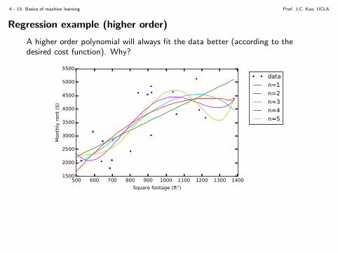
Regression example (higher order)
A higher order polynomial will always fit the data better (according to thedesired cost function). Why?
500 600 700 800 900 1000 1100 1200 1300 1400
Square footage (ft2)
1500
2000
2500
3000
3500
4000
4500
5000
5500
Month
ly r
ent
($)
data
n=1
n=2
n=3
n=4
n=5
4 - 14: Basics of machine learning Prof. J.C. Kao, UCLA
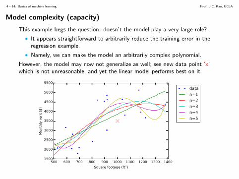
Model complexity (capacity)
This example begs the question: doesn’t the model play a very large role?
• It appears straightforward to arbitrarily reduce the training error in theregression example.
• Namely, we can make the model an arbitrarily complex polynomial.
However, the model may now not generalize as well; see new data point ’x’which is not unreasonable, and yet the linear model performs best on it.
500 600 700 800 900 1000 1100 1200 1300 1400
Square footage (ft2)
1500
2000
2500
3000
3500
4000
4500
5000
5500
Month
ly r
ent
($)
data
n=1
n=2
n=3
n=4
n=5
4 - 15: Basics of machine learning Prof. J.C. Kao, UCLA
Overfitting
This idea of generalization can be made more formal by introducing theconcepts of a training set and testing set.
• Training data is data that is used to learn the parameters of your model.
• Testing data is data that is excluded in training and used to score yourmodel.
There is also a notion of validation data, which we will get to later.
A model which has very low training error but high testing error is called overfit.

4 - 16: Basics of machine learning Prof. J.C. Kao, UCLA
Larger datasets ameliorate overfitting
While overfitting may arise due to an overly complex model, it can be helpedby incorporating more training data.
400 600 800 1000 1200 1400 1600
Square footage (ft2)
0
1000
2000
3000
4000
5000
6000
7000
8000
Month
ly r
ent
($)
data
n=1
n=2
n=3
n=4
n=5
This suggests that when a lot of data is available, it may be appropriate to usemore complex models. (Another technique we will discuss later, regularization,also helps with overfitting.) This is a shadow of things to come (i.e., neuralnetworks which have large complexity).
4 - 17: Basics of machine learning Prof. J.C. Kao, UCLA
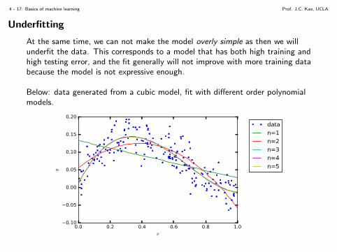
Underfitting
At the same time, we can not make the model overly simple as then we willunderfit the data. This corresponds to a model that has both high training andhigh testing error, and the fit generally will not improve with more training databecause the model is not expressive enough.
Below: data generated from a cubic model, fit with different order polynomialmodels.
0.0 0.2 0.4 0.6 0.8 1.0x
0.10
0.05
0.00
0.05
0.10
0.15
0.20
y
data
n=1
n=2
n=3
n=4
n=5

4 - 18: Basics of machine learning Prof. J.C. Kao, UCLA
Estimators
The notions of underfitting and overfitting are closely related to two otherconcepts: bias and variance. The bias and variance quantify importantstatistics about an estimator.
What is an estimator?
• Assume, for now, that there is a set of parameters given by θ.
• The estimator, θ, is a single “best” estimate of θ. (Note that we are notestimating the distribution of θ. We are treating θ as taking on a singlevalue.)
• Given a training set of m iid examples, x(1),x(2), . . . ,x(m), the estimatormay be generally defined as:
θm = g(x(1), . . . ,x(m))
• θm ought be treated as a random variable, as we achieve an estimate of itthrough the random samples we have as training data.

4 - 19: Basics of machine learning Prof. J.C. Kao, UCLA
Estimator bias
The bias of an estimator, θm, is defined as:
bias(θm) = E(θm)− θ
Note:
• The expectation is taken over the data (where the randomness isintroduced through samples x(i)).
• Informally, the bias measures how close θm comes to estimating θ onaverage.
• An estimator is called unbiased if bias(θm) = 0.
• An estimator is called asymptotically unbiased if limm→∞ E(θm) = θ, i.e.,bias(θm)→ 0.

4 - 20: Basics of machine learning Prof. J.C. Kao, UCLA
Estimator bias (example)
Let {x(1), x(2), . . . , x(m)} be iid samples from a Bernoulli distribution withmean θ. The sample mean estimator is given by:
θm =1
m
m∑i=1
x(i)
Then, the bias of this estimator is:
bias(θm) = E
(1
m
m∑i=1
x(i))− θ
=1
m
m∑i=1
Ex(i) − θ
=1
m
m∑i=1
θ − θ
= 0
where we used the fact that
Ex(i) =∑
x(i)∈{0,1}
x(i)p(x(i)) =∑
x(i)∈{0,1}
x(i)θx(i)
(1− θ)(1−x(i))
4 - 21: Basics of machine learning Prof. J.C. Kao, UCLA
Estimator variance
An unbiased estimator may on average estimate θ, but any single instance of θmay deviate from θ. The variance of θ in predicting is called the variance of theestimator, denoted var(θ).
Some notes:
• This variability is due to the data samples that you get.
• The standard error of the estimator is√
var(θ) and is commonly denoted
SE(θ).

4 - 22: Basics of machine learning Prof. J.C. Kao, UCLA
Estimator variance (example)
Let {x(1), x(2), . . . , x(m)} be iid samples from a Bernoulli distribution withmean θ. The sample mean estimator is given by:
θm =1
m
m∑i=1
x(i)
Then, the variance of this estimator is:
var(θm) = var
(1
m
m∑i=1
x(i))
=1
m2
m∑i=1
var(x(i))
=1
m2
m∑i=1
θ(1− θ)
=θ(1− θ)
m
4 - 23: Basics of machine learning Prof. J.C. Kao, UCLA
Estimator variance (example)
A common metric used in evaluating the average of the data is the standarderror of the mean. Given iid samples x(1), . . . , x(m), the standard error of themean is given by:
SE(µm) =
√√√√var
(1
m
m∑i=1
x(i)
)
=
√√√√ 1
m2
m∑i=1
var(x(i))
=
√1
m2mvar(x(i))
=σ√m
What does this mean intuitively?
4 - 24: Basics of machine learning Prof. J.C. Kao, UCLA
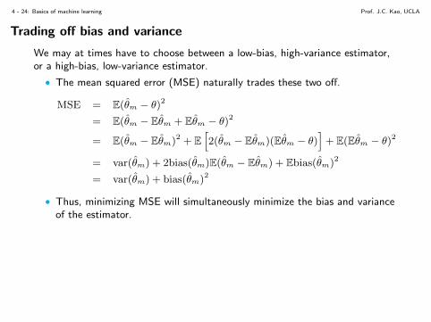
Trading off bias and variance
We may at times have to choose between a low-bias, high-variance estimator,or a high-bias, low-variance estimator.
• The mean squared error (MSE) naturally trades these two off.
MSE = E(θm − θ)2
= E(θm − Eθm + Eθm − θ)2
= E(θm − Eθm)2 + E[2(θm − Eθm)(Eθm − θ)
]+ E(Eθm − θ)2
= var(θm) + 2bias(θm)E(θm − Eθm) + Ebias(θm)2
= var(θm) + bias(θm)2
• Thus, minimizing MSE will simultaneously minimize the bias and varianceof the estimator.

4 - 25: Basics of machine learning Prof. J.C. Kao, UCLA
Model capacity, bias and variance
When we measure the performance of an estimator via MSE ...• ... a model that underfits the data has high bias.• ... a model that overfits the data has high variance.
Mod
el e
rror
Model capacity (complexity)
estimatorbias
estimatorvariance
generalization error
overfittingunderfitting

4 - 26: Basics of machine learning Prof. J.C. Kao, UCLA
Choosing a model
Thus, we arrive at a problem. How can we select the best model if these canbe made arbitrarily complex?
• In the scenario where no data was set aside and we must make anevaluation on the training data only, this is the problem of model selection.There are criterion which penalize the model complexity. For example ...
• Akaike information criterion (AIC)• Bayes information criterion (BIC)• Deviance informaiton criterion (DIC)• We won’t cover these in class.
• More typically, we leave aside data that was not used in training, orgenerate new data. We then test our model on this non-training set data,and evaluate the model’s performance.

4 - 27: Basics of machine learning Prof. J.C. Kao, UCLA
Training, validation, and testing data
The standard for training, evaluating, and choosing models is to use differentdatasets for each step.
• Training data is data that is used to learn the parameters of your model.
• Validation data is data that is used to optimize the hyperparameters ofyour model. This avoids the potential of overfitting to nuances in thetesting dataset.
• Testing data is data that is used to score your model.
Note, in many cases, testing and validation datasets are used interchangeablyas datasets that are used to evaluate the model. In this scenario,hyperparameters would also be optimized using training data.

4 - 28: Basics of machine learning Prof. J.C. Kao, UCLA
k-fold cross validation
In a common scenario, you will be given a training dataset and a testingdataset. To train a model using this dataset, one common approach is k-foldcross validation. Then the procedure looks as follows:
• Let the training dataset contain N examples.
• Then, split the data into k equal sets, each of N/k examples. Each ofthese sets is called a “fold.”
• k− 1 of the folds are datasets that are used to train the model parameters.
• The remaining fold is a testing dataset used to evaluate the model.
• You may repeatedly train the model by choosing which folds comprise thetraining folds and the testing fold.

4 - 29: Basics of machine learning Prof. J.C. Kao, UCLA
k-fold cross validation
The following picture is appropriate for k-fold cross-validation. Green denotestraining data, red denotes testing data, and yellow denotes validation data.
Original data
k-fold cross-validation with no hyperparameters
Fold 1 Fold 2 Fold 3 Fold 4 Fold 5
k-fold cross-validation with hyperparameters
Training fold Test fold
Fold 1 Fold 2 Fold 3 Fold 4 Test fold
In practice, k-fold cross-validation may be expensive and hence not appropriate.
4 - 30: Basics of machine learning Prof. J.C. Kao, UCLA
Other types of optimization
We’ve talked about examples where we want to minimize a mean-square erroror distance metric.
Another metric that we may want to minimize is the probability of havingobserved the data. In this framework, the data is modeled to have somedistribution with parameters. We choose the parameters to maximize theprobability of having observed our training data.

4 - 31: Basics of machine learning Prof. J.C. Kao, UCLA
Example of ML estimation
Say we receive paired data {x(i), y(i)} where x(i) ∈ R2 is a data point thatbelongs to one of three classes, y(i) ∈ {1, 2, 3}. Classes 1, 2, 3 denote the threepossible classes (or labels) that a data point could belong to. The drawingbelow (with appropriate labels) represents this:
0.5 0.0 0.5 1.0 1.5 2.0 2.5 3.0 3.50.0
0.5
1.0
1.5
2.0
2.5
3.0
4 - 32: Basics of machine learning Prof. J.C. Kao, UCLA
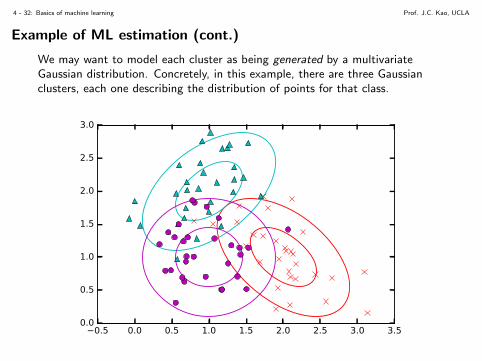
Example of ML estimation (cont.)
We may want to model each cluster as being generated by a multivariateGaussian distribution. Concretely, in this example, there are three Gaussianclusters, each one describing the distribution of points for that class.
0.5 0.0 0.5 1.0 1.5 2.0 2.5 3.0 3.50.0
0.5
1.0
1.5
2.0
2.5
3.0
4 - 33: Basics of machine learning Prof. J.C. Kao, UCLA
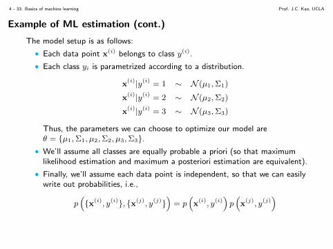
Example of ML estimation (cont.)
The model setup is as follows:
• Each data point x(i) belongs to class y(i).
• Each class yi is parametrized according to a distribution.
x(i)|y(i) = 1 ∼ N (µ1,Σ1)
x(i)|y(i) = 2 ∼ N (µ2,Σ2)
x(i)|y(i) = 3 ∼ N (µ3,Σ3)
Thus, the parameters we can choose to optimize our model areθ = {µ1,Σ1, µ2,Σ2, µ3,Σ3}.
• We’ll assume all classes are equally probable a priori (so that maximumlikelihood estimation and maximum a posteriori estimation are equivalent).
• Finally, we’ll assume each data point is independent, so that we can easilywrite out probabilities, i.e.,
p({x(i), y(i)}, {x(j), y(j)}
)= p
(x(i), y(i)
)p(x(j), y(j)
)
4 - 34: Basics of machine learning Prof. J.C. Kao, UCLA
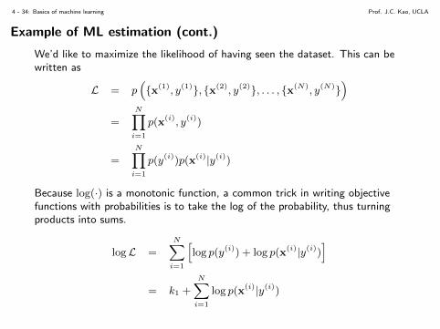
Example of ML estimation (cont.)
We’d like to maximize the likelihood of having seen the dataset. This can bewritten as
L = p({x(1), y(1)}, {x(2), y(2)}, . . . , {x(N), y(N)}
)=
N∏i=1
p(x(i), y(i))
=N∏i=1
p(y(i))p(x(i)|y(i))
Because log(·) is a monotonic function, a common trick in writing objectivefunctions with probabilities is to take the log of the probability, thus turningproducts into sums.
logL =N∑i=1
[log p(y(i)) + log p(x(i)|y(i))
]= k1 +
N∑i=1
log p(x(i)|y(i))
4 - 35: Basics of machine learning Prof. J.C. Kao, UCLA
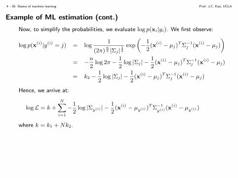
Example of ML estimation (cont.)
Now, to simplify the probabilities, we evaluate log p(xi|yi). We first observe:
log p(x(i)|y(i) = j) = log1
(2π)n2 |Σj |
12
exp
(−1
2(x(i) − µj)
T Σ−1j (x(i) − µj)
)= −n
2log 2π − 1
2log |Σj | −
1
2(x(i) − µj)
T Σ−1j (x(i) − µj)
= k2 −1
2log |Σj | −
1
2(x(i) − µj)
T Σ−1j (x(i) − µj)
Hence, we arrive at:
logL = k +
N∑i=1
−1
2log |Σy(i) | −
1
2(x(i) − µy(i))
T Σ−1
y(i)(x(i) − µy(i))
where k = k1 +Nk2.

4 - 36: Basics of machine learning Prof. J.C. Kao, UCLA
Examle of ML estimation (cont.)
Let’s then find the optimal parameters by differentiating and setting to zero.First, we find the optimal µj . We note that only the last term in the loglikelihood has µj terms in instances where y(i) = j.
∂ logL∂µj
=∂
∂µj
∑i:y(i)=j
−1
2(x(i) − µj)
T Σ−1j (x(i) − µj)
= −1
2
∂
∂µj
∑i:y(i)=j
(x(i))T Σ−1j x(i) − 2µT
j Σ−1j x(i) + µT
j Σ−1j µj)
= −1
2
∑i:y(i)=j
−2Σ−1j x(i) + 2Σ−1
j µj
Setting the derivative to zero, we have that:
µj =1
Nj
∑i:y(i)=j
x(i)
where Nj =∑
i:y(i)=j 1, i.e., the number of training examples where y(i) = j.Does this answer make sense?

4 - 37: Basics of machine learning Prof. J.C. Kao, UCLA
Examle of ML estimation (cont.)
We next take the derivative with respect to Σ, using the following facts (formore information, see “Tools” lecture notes on derivatives w.r.t. matrices):
∂
∂Σtr(Σ−1A) = −Σ−TAT Σ−T
∂
∂Σlog |Σ| = Σ−T
Now, differentiating:
∂ logL∂Σj
=∂
∂Σj
∑i:y(i)=j
−1
2log |Σj | −
1
2(x(i) − µj)
T Σ−1j (x(i) − µj)
= −1
2
∂
∂Σj
∑i:y(i)=j
log |Σj |+ tr(
(x(i) − µj)T Σ−1
j (x(i) − µj))
= −1
2
∂
∂Σj
∑i:y(i)=j
log |Σj |+ tr(
Σ−1j (x(i) − µj)(x
(i) − µj)T)
= −1
2
∑i:y(i)=j
Σ−Tj − Σ−T
j (x(i) − µj)(x(i) − µj)
T Σ−Tj
4 - 38: Basics of machine learning Prof. J.C. Kao, UCLA
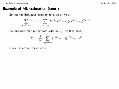
Example of ML estimation (cont.)
Setting the derivative equal to zero, we arrive at:∑i:y(i)=j
Σ−1j =
∑i:y(i)=j
Σ−1j (x(i) − µj)(x
(i) − µj)T Σ−1
j
Pre and post-multiplying both sides by Σj , we then have:
Σj =1
Nj
∑i:y(i)=j
(x(i) − µj)(x(i) − µj)
T
Does this answer make sense?

4 - 39: Basics of machine learning Prof. J.C. Kao, UCLA
Example of ML estimation (cont.)
Solving for the optimal parameters µj and Σj for all classes, we arrive at thefollowing solution:
0.5 0.0 0.5 1.0 1.5 2.0 2.5 3.0 3.50.0
0.5
1.0
1.5
2.0
2.5
3.0

4 - 40: Basics of machine learning Prof. J.C. Kao, UCLA
Example of ML estimation (cont.)
Imagine now a new point x comes in that we’d like to classify as being in oneof three classes. To do so, we’d like to calculate: Pr(y = j|x) and pick the jthat maximizes this probability. We’ll denote this probability p(j|x). We’ll alsoassume, as earlier, that the classes are equally probable, i.e., Pr(y = j) is thesame for all j.
arg maxj
p(j|x) = arg maxj
p(x|j)p(j)p(x)
= arg maxj
p(x|j)p(j)
= arg maxj
log p(x|j)
= arg maxj
[− log |Σj | − (x− µj)
T Σ−1j (x− µj)
]

4 - 41: Basics of machine learning Prof. J.C. Kao, UCLA
Example of ML estimation (cont.)
This classification rule results in the following classifier:

4 - 42: Basics of machine learning Prof. J.C. Kao, UCLA
Even more cost functions
There are even more cost functions that we could use. We’ll encounter someothers in this class. Others include:
• MAP estimation.
• KL divergence.
• Maximize an approximation of the distribution.
In machine learning, it is important to arrive at an appropriate model and costfunction. After that, it’s important to know how to optimize it. In ourexamples here, the cost functions were simple enough (i.e., quadratic in theparameters) that we could differentiate and set the derivative equal to zero. Infuture lectures, we’ll discuss more general ways to learn parameters of modelswhen they are not so simple.