Embed Size (px)
Citation preview
36106 Managerial Decision ModelingLinear Decision Models: Part II
Kipp MartinUniversity of Chicago
Booth School of Business
January 20, 2014
1
Reading and Excel Files
Reading (Powell and Baker):
I Sections 9.3-9.6
I Section 9.8
Files used in this lecture:
I simpleLP.xlsx
2
Lecture Outline
Constrained Optimization
Optimization Categories
Optimization Concepts
Solution Report
Vocabulary
3
Constrained Optimization
Google the word optimization and you get over 62 million links,Googling optimal gives about 70 million links.
Words such as optimal and optimization mean different things todifferent people. In this class they take on a precise meaning.
We will devote a lot of time this quarter to building optimizationmodels and implementing them in Excel.
Before we can build some neat applications and learn some really usefulstuff, we need a few basic math concepts.
You need to understand the concepts: objective function, constraint,feasible, variable, parameter, and optimal.
4
Constrained Optimization
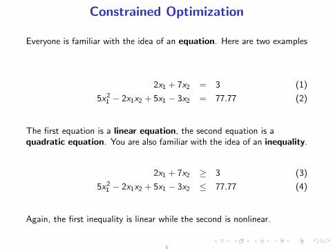
Everyone is familiar with the idea of an equation. Here are two examples
2x1 + 7x2 = 3 (1)
5x21 − 2x1x2 + 5x1 − 3x2 = 77.77 (2)
The first equation is a linear equation, the second equation is aquadratic equation. You are also familiar with the idea of an inequality.
2x1 + 7x2 ≥ 3 (3)
5x21 − 2x1x2 + 5x1 − 3x2 ≤ 77.77 (4)
Again, the first inequality is linear while the second is nonlinear.
5
Constrained Optimization
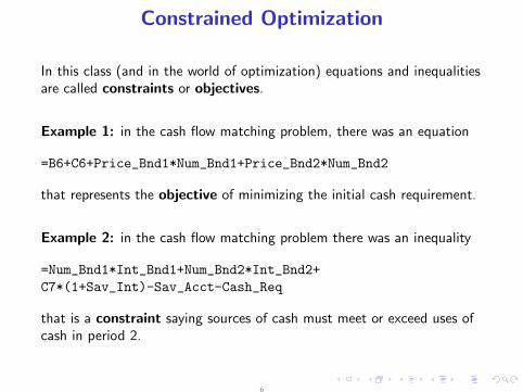
In this class (and in the world of optimization) equations and inequalitiesare called constraints or objectives.
Example 1: in the cash flow matching problem, there was an equation
=B6+C6+Price_Bnd1*Num_Bnd1+Price_Bnd2*Num_Bnd2
that represents the objective of minimizing the initial cash requirement.
Example 2: in the cash flow matching problem there was an inequality
=Num_Bnd1*Int_Bnd1+Num_Bnd2*Int_Bnd2+
C7*(1+Sav_Int)-Sav_Acct-Cash_Req
that is a constraint saying sources of cash must meet or exceed uses ofcash in period 2.
6
Constrained Optimization
Every constrained optimization problem has an objective function that ismaximized or minimized subject to constraints.
In the cash flow matching problem the objective is to minimize the initialamount of cash required subject to constraints that require the sources ofcash to meet the uses of cash.
In the Markowitz portfolio optimization we study later the objective is tominimize the variablity of a stock portfolio subject to a constraint on therequired return of the portfolio.
In the airline revenue management problem we study later the objectiveis to maximize revenue subject to constraints of the seats available invarious categories.
Definition: the variables in the constraints and objective are calleddecision variables.
7
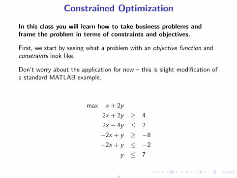
Constrained Optimization
In this class you will learn how to take business problems andframe the problem in terms of constraints and objectives.
First, we start by seeing what a problem with an objective function andconstraints look like.
Don’t worry about the application for now – this is slight modification ofa standard MATLAB example.
max x + 2y
2x + 2y ≥ 4
2x − 4y ≤ 2
−2x + y ≥ −8
−2x + y ≤ −2
y ≤ 7
8

Constrained Optimization
Here is the feasible region of a simple two-variable constrainedoptimization problem.
Attempting a What-If analysis by picking feasible points is simply notefficient!
9
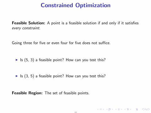
Constrained Optimization
Feasible Solution: A point is a feasible solution if and only if it satisfiesevery constraint.
Going three for five or even four for five does not suffice.
I Is (5, 3) a feasible point? How can you test this?
I Is (3, 5) a feasible point? How can you test this?
Feasible Region: The set of feasible points.
10
Constrained Optimization
In this example, there are an infinite number of feasible solutions.
We want the best or optimal solution.
A solution is an optimal solution to a maximization problem if there isno feasible solution that has a strictly larger objective function value.
A solution is an optimal solution to a minimization problem if there isno feasible solution that has a strictly smaller objective function value.
11
Constrained Optimization
In practice, optimization problems may involve thousands or even millionsof variables and constraints.
These large problems are solved using optimization software codes whichare often called solvers. The Excel Solver is one such example.
There are numerous optimization solvers, both commercial and opensource.
Solvers work by finding a feasible point and then move in an improvingdirection (where the objective gets bigger in case of a maximization).Then a step is taken in the direction of improvement and the processrepeats.
Finding improving directions and moving in the direction of improvementcan be mathematically complex. We won’t worry about this. We letExcel worry about this and do all the work.
12
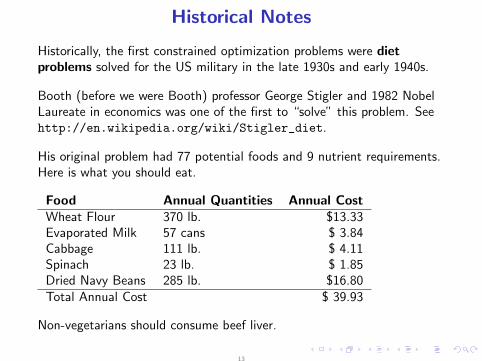
Historical Notes
Historically, the first constrained optimization problems were dietproblems solved for the US military in the late 1930s and early 1940s.
Booth (before we were Booth) professor George Stigler and 1982 NobelLaureate in economics was one of the first to “solve” this problem. Seehttp://en.wikipedia.org/wiki/Stigler_diet.
His original problem had 77 potential foods and 9 nutrient requirements.Here is what you should eat.
Food Annual Quantities Annual CostWheat Flour 370 lb. $13.33Evaporated Milk 57 cans $ 3.84Cabbage 111 lb. $ 4.11Spinach 23 lb. $ 1.85Dried Navy Beans 285 lb. $16.80Total Annual Cost $ 39.93
Non-vegetarians should consume beef liver.
13
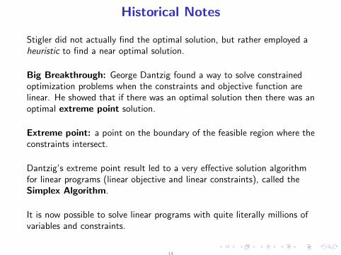
Historical Notes
Stigler did not actually find the optimal solution, but rather employed aheuristic to find a near optimal solution.
Big Breakthrough: George Dantzig found a way to solve constrainedoptimization problems when the constraints and objective function arelinear. He showed that if there was an optimal solution then there was anoptimal extreme point solution.
Extreme point: a point on the boundary of the feasible region where theconstraints intersect.
Dantzig’s extreme point result led to a very effective solution algorithmfor linear programs (linear objective and linear constraints), called theSimplex Algorithm.
It is now possible to solve linear programs with quite literally millions ofvariables and constraints.
14
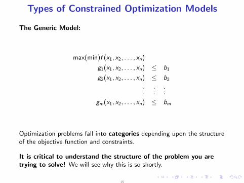
Types of Constrained Optimization Models
The Generic Model:
max(min)f (x1, x2, . . . , xn)
g1(x1, x2, . . . , xn) ≤ b1
g2(x1, x2, . . . , xn) ≤ b2...
......
gm(x1, x2, . . . , xn) ≤ bm
Optimization problems fall into categories depending upon the structureof the objective function and constraints.
It is critical to understand the structure of the problem you aretrying to solve! We will see why this is so shortly.
15
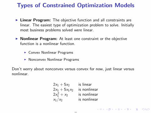
Types of Constrained Optimization Models
I Linear Program: The objective function and all constraints arelinear. The easiest type of optimization problem to solve. Initiallymost business problems solved were linear.
I Nonlinear Program: At least one constraint or the objectivefunction is a nonlinear function.
I Convex Nonlinear Programs
I Nonconvex Nonlinear Programs
Don’t worry about nonconvex versus convex for now, just linear versusnonlinear.
2x1 + 5x2 is linear2x1 + 5x1x2 is nonlinear2x21 + x2 is nonlinearx1/x2 is nonlinear
16
Types of Constrained Optimization Models
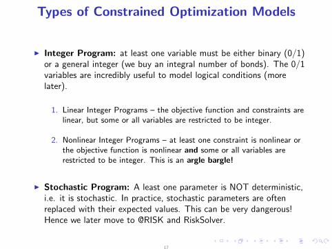
I Integer Program: at least one variable must be either binary (0/1)or a general integer (we buy an integral number of bonds). The 0/1variables are incredibly useful to model logical conditions (morelater).
1. Linear Integer Programs – the objective function and constraints arelinear, but some or all variables are restricted to be integer.
2. Nonlinear Integer Programs – at least one constraint is nonlinear orthe objective function is nonlinear and some or all variables arerestricted to be integer. This is an argle bargle!
I Stochastic Program: A least one parameter is NOT deterministic,i.e. it is stochastic. In practice, stochastic parameters are oftenreplaced with their expected values. This can be very dangerous!Hence we later move to @RISK and RiskSolver.
17
Types of Constrained Optimization Models
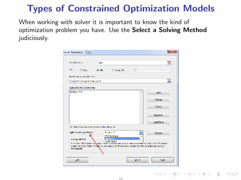
When working with solver it is important to know the kind ofoptimization problem you have. Use the Select a Solving Methodjudiciously.
18
Types of Constrained Optimization Models
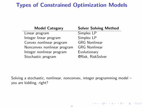
Model Category Solver Solving MethodLinear program Simplex LPInteger linear program Simplex LPConvex nonlinear program GRG NonlinearNonconvex nonlinear program GRG NonlinearInteger nonlinear program EvolutionaryStochastic program @Risk, RiskSolver
Solving a stochastic, nonlinear, nonconvex, integer programming model –you are kidding, right?
19
Types of Constrained Optimization Models
A Few Excel Hints:
1. Assume you have a formula in cell A2 which is = A1 ∗ B1. At firstglance, this is a nonlinear expression. However, if for example, cell A1 has= 7, then Excel will make this substitution into A2 and the formula in A2
is really =7*B1 which is linear in B1.
After substitutions, ideally there are no cells with nonlinear relationshipsinvolving adjustable cells!
2. Functions are dangerous! Consider the following use of the IF
function in mpfpHotFudge.xlsx.
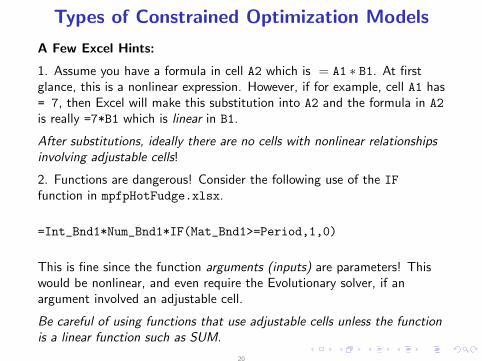
=Int_Bnd1*Num_Bnd1*IF(Mat_Bnd1>=Period,1,0)
This is fine since the function arguments (inputs) are parameters! Thiswould be nonlinear, and even require the Evolutionary solver, if anargument involved an adjustable cell.
Be careful of using functions that use adjustable cells unless the functionis a linear function such as SUM.
20
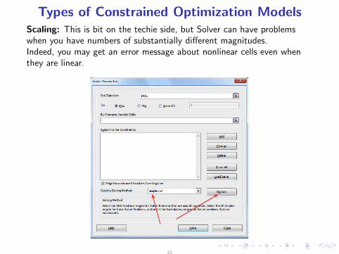
Types of Constrained Optimization ModelsScaling: This is bit on the techie side, but Solver can have problemswhen you have numbers of substantially different magnitudes.Indeed, you may get an error message about nonlinear cells even whenthey are linear.
21
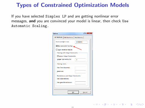
Types of Constrained Optimization Models
If you have selected Simplex LP and are getting nonlinear errormessages, and you are convinced your model is linear, then check Use
Automatic Scaling.
22
Optimization Concepts
Something new to worry about in the nonlinear world – the software findsa local optimum. First, the global concept.
A point x is a global maximum of f (x) if and only if
f (x) ≥ f (x) for all x
A point x is a global minimum of f (x) if and only if
f (x) ≤ f (x) for all x
23
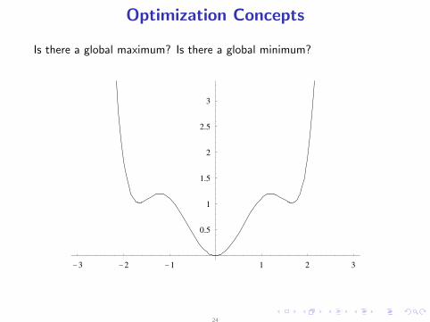
Optimization Concepts
Is there a global maximum? Is there a global minimum?
-3 -2 -1 1 2 3
0.5
1
1.5
2
2.5
3
24
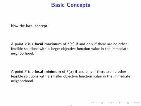
Basic Concepts
Now the local concept.
A point x is a local maximum of f (x) if and only if there are no otherfeasible solutions with a larger objective function value in the immediateneighborhood.
A point x is a local minimum of f (x) if and only if there are no otherfeasible solutions with a smaller objective function value in the immediateneighborhood.
25
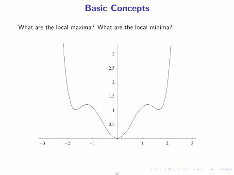
Basic Concepts
What are the local maxima? What are the local minima?
-3 -2 -1 1 2 3
0.5
1
1.5
2
2.5
3
26
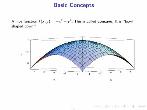
Basic Concepts
A nice function f (x , y) = −x2 − y2. This is called concave. It is “bowlshaped down.”
-4 -2 0 2 4
X
-4-2024
Y
-40
-20
0
Z
0 2 4
27
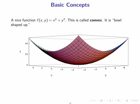
Basic Concepts
A nice function f (x , y) = x2 + y2. This is called convex. It is “bowlshaped up.”
-4 -2 0 2 4
X
-4-2024
Y
0
20
40
Z
0 2 4
28
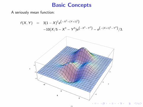
Basic ConceptsA seriously mean function:
f (X ,Y ) = 3(1− X )2e(−X 2−(Y+1)2)
−10(X/5− X 3 − Y 5)e(−X 2−Y 2) − e(−(X+1)2−Y 2)/3.
-2
0
2
X-2
0
2
Y
-5
0
5
Z
-2
0
2
X
29
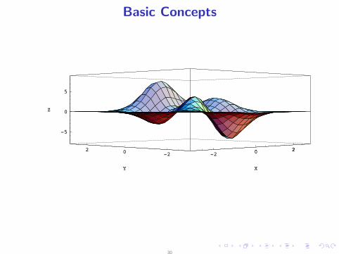
Basic Concepts
-2 0 2
X
-202
Y
-5
0
5
Z
0 2
30
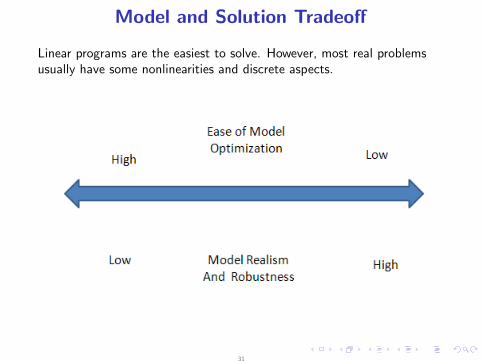
Model and Solution Tradeoff
Linear programs are the easiest to solve. However, most real problemsusually have some nonlinearities and discrete aspects.
31
Model and Solution Tradeoff
Even now, the most commonly solved problems are deterministicmixed-integer linear programs.
Is the world linear? I don’t think so!
Question: So why all the solving of mixed integer linear programs?
Answer: Say’s Law!
32
Solution Report
When you “solve” an optimization problem using a solver, you get asolution report.
This solution report will indicate whether or not it found an optimalsolution.
If an optimal solution is found, the solution report will give the optimalobjective function value and will give the optimal values of the decisionvariables.
The solution report also provides other information given in Chapter 9, inparticular Appendix 9.1.
33
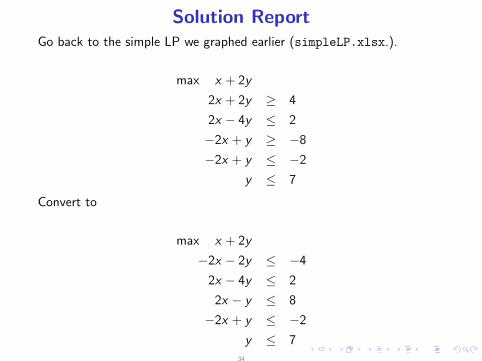
Solution ReportGo back to the simple LP we graphed earlier (simpleLP.xlsx.).
max x + 2y
2x + 2y ≥ 4
2x − 4y ≤ 2
−2x + y ≥ −8
−2x + y ≤ −2
y ≤ 7
Convert to
max x + 2y
−2x − 2y ≤ −4
2x − 4y ≤ 2
2x − y ≤ 8
−2x + y ≤ −2
y ≤ 7
34
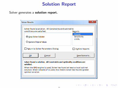
Solution Report
Solver generates a solution report.
35
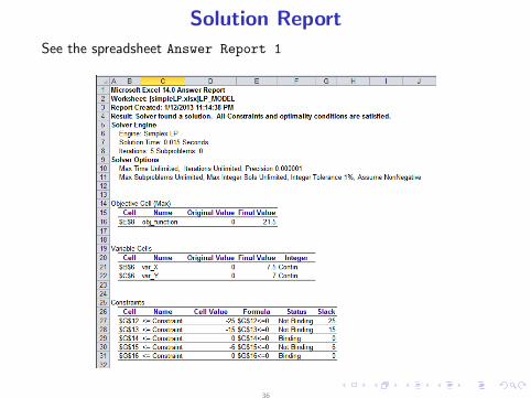
Solution Report
See the spreadsheet Answer Report 1
36
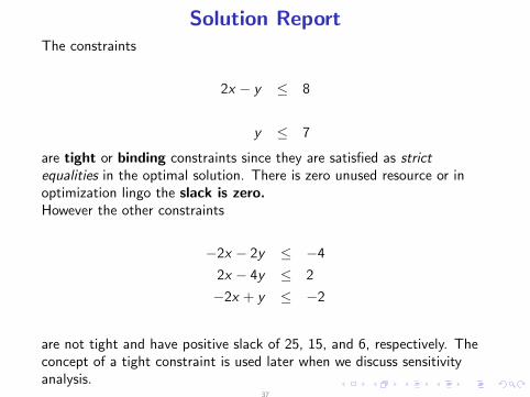
Solution ReportThe constraints
2x − y ≤ 8
y ≤ 7
are tight or binding constraints since they are satisfied as strictequalities in the optimal solution. There is zero unused resource or inoptimization lingo the slack is zero.However the other constraints
−2x − 2y ≤ −4
2x − 4y ≤ 2
−2x + y ≤ −2
are not tight and have positive slack of 25, 15, and 6, respectively. Theconcept of a tight constraint is used later when we discuss sensitivityanalysis.
37
Solution Report
Note also that the optimal solution of x = 7.5 and y = 7 with optimalsolution value of 21.5 is:
I on the boundary of the feasible region,
I and it is at the intersection of two or more constraints – a cornerpoint
Linear programming software only searches for extreme point solutions.
38
Solution Report
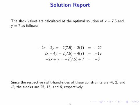
The slack values are calculated at the optimal solution of x = 7.5 andy = 7 as follows:
−2x − 2y = −2(7.5) − 2(7) = −29
2x − 4y = 2(7.5) − 4(7) = −13
−2x + y = −2(7.5) + 7 = −8
Since the respective right-hand-sides of these constraints are -4, 2, and-2, the slacks are 25, 15, and 6, respectively.
39
Solution Possibilities
A constrained optimization problem either has an optimal solution or itdoes not.
If it has an optimal solution, then it has a unique optimal solution oralternative optima.
What is the graphical interpretation of alternative optima?
If it does not have an optimal solution, then in the linear case it isunbounded or infeasible.
40
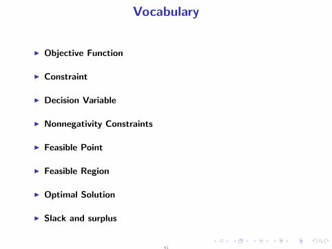
Vocabulary
I Objective Function
I Constraint
I Decision Variable
I Nonnegativity Constraints
I Feasible Point
I Feasible Region
I Optimal Solution
I Slack and surplus
41
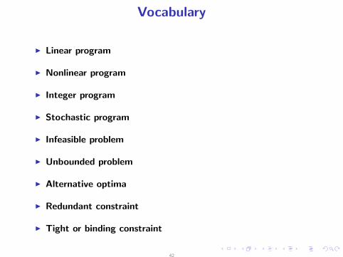
Vocabulary
I Linear program
I Nonlinear program
I Integer program
I Stochastic program
I Infeasible problem
I Unbounded problem
I Alternative optima
I Redundant constraint
I Tight or binding constraint
42