Embed Size (px)
Citation preview
344 IEEE TRANSACTIONS ON NEURAL NETWORKS AND LEARNING SYSTEMS, VOL. 25, NO. 2, FEBRUARY 2014
Nanophotonic Reservoir Computing With PhotonicCrystal Cavities to Generate Periodic Patterns
Martin Andre Agnes Fiers, Member, IEEE, Thomas Van Vaerenbergh, Student Member, IEEE,Francis Wyffels, David Verstraeten, Benjamin Schrauwen, Joni Dambre, Member, IEEE,
and Peter Bienstman, Member, IEEE
Abstract— Reservoir computing (RC) is a technique in machinelearning inspired by neural systems. RC has been used suc-cessfully to solve complex problems such as signal classificationand signal generation. These systems are mainly implementedin software, and thereby they are limited in speed and powerefficiency. Several optical and optoelectronic implementationshave been demonstrated, in which the system has signals withan amplitude and phase. It is proven that these enrich thedynamics of the system, which is beneficial for the performance.In this paper, we introduce a novel optical architecture based onnanophotonic crystal cavities. This allows us to integrate manyneurons on one chip, which, compared with other photonic solu-tions, closest resembles a classical neural network. Furthermore,the components are passive, which simplifies the design andreduces the power consumption. To assess the performance ofthis network, we train a photonic network to generate periodicpatterns, using an alternative online learning rule called first-order reduced and corrected error. For this, we first train aclassical hyperbolic tangent reservoir, but then we vary someof the properties to incorporate typical aspects of a photonicsreservoir, such as the use of continuous-time versus discrete-time signals and the use of complex-valued versus real-valuedsignals. Then, the nanophotonic reservoir is simulated and weexplore the role of relevant parameters such as the topology, thephases between the resonators, the number of nodes that arebiased and the delay between the resonators. It is importantthat these parameters are chosen such that no strong self-oscillations occur. Finally, our results show that for a signalgeneration task a complex-valued, continuous-time nanophotonicreservoir outperforms a classical (i.e., discrete-time, real-valued)leaky hyperbolic tangent reservoir (normalized root-mean-squareerrors = 0.030 versus NRMSE = 0.127).
Index Terms— Integrated optics, optical neural network,pattern generation, photonic reservoir computing, supervisedlearning.
Manuscript received August 16, 2012; revised June 4, 2013; acceptedJuly 20, 2013. Date of publication August 15, 2013; date of current versionJanuary 10, 2014. This work was supported in part by the InteruniversityAttraction Pole Photonics@be program of the Belgian Science Policy Officeand the ERC NaResCo Starting grant. The work of M. Fiers was supportedby a research fund of Ghent University. The work of T. Van Vaerenbergh wassupported by the Flemish Research Foundation under a Ph.D. grant.
M. A. A. Fiers, T. Van Vaerenbergh, and P. Bienstman are with theDepartment of Information Technology of Ghent University, Ghent 9000,Belgium, and also with the Center for Nano and Biophotonics, GhentUniversity, Ghent B-9000, Belgium (e-mail: [email protected];[email protected]; [email protected]).
F. Wyffels, D. Verstraeten, B. Schrauwen, and J. Dambre are withthe ELIS Department, Ghent University, Ghent 9000, Belgium (e-mail:[email protected]; [email protected]; [email protected]; [email protected]).
Color versions of one or more of the figures in this paper are availableonline at http://ieeexplore.ieee.org.
Digital Object Identifier 10.1109/TNNLS.2013.2274670
I. INTRODUCTION
RESERVOIR computing (RC) is a recently proposedmethodology in the field of machine learning [1], [2].
Originally, it combined a recurrent neural network (RNN) witha linear readout layer, trained on the neuron states. The RNNitself, usually consisting of nonlinear neurons, is left untrained.It transforms the input signal to a high-dimensional state space,containing many linear and nonlinear transformations of theinput history. Only a few global parameters, such as the overallgain in the system, the magnitude of the inputs, and thenetwork size are optimized to tune the reservoir dynamicsinto an appropriate regime for the task at hand. RC performsvery well on a variety of tasks, e.g., speech recognition [3],detection of epileptic seizures [4], robot localization [5], andtime series prediction [1], [6].
Typically, a reservoir is implemented as a sequential algo-rithm in software. This obviously limits the speed of operationof the reservoir. The inherent parallelism of the neural networkconcept makes it a good candidate for parallel hardware imple-mentations. In particular, analog hardware platforms in whichthe nonlinearity is provided by the physics of the componentscan be very efficient. A good overview of hardware implemen-tations of RC can be found in [7]. In the electronic domain,there are implementations such as an FPGA [3] and VLSI [8].Recently, photonic and optoelectronic implementations of RChave been demonstrated [9], [10]. An advantage of photonicimplementations is the fact that they can be operated in acoherent regime, where all signals have both an amplitude anda phase, which interact whenever signals are combined. Thisincreases the dimensionality of the state space. Even whenthe number of observed signals remains unchanged (e.g., onlythe magnitudes of the neuron states), it generally enriches therealized projection of the input into the observed portion ofstate space, yielding better reservoirs. Furthermore, the veryhigh carrier frequency of optical signals, which can be carriedover dielectrical materials with low loss, allows the system toprocess signals faster, and potentially with lower power, thanelectronic implementations.
Vandoorne et al. [10] demonstrated, through simulations,that RC with an integrated circuit of semiconductor opticalamplifiers (SOAs) as a reservoir can solve a speech recogni-tion task with state-of-the-art performance. These componentsare, however, relatively large and, because they are activeamplifiers, the network consumes a lot of power. Here, we
2162-237X © 2013 IEEE. Personal use is permitted, but republication/redistribution requires IEEE permission.See http://www.ieee.org/publications_standards/publications/rights/index.html for more information.
FIERS et al.: NANOPHOTONIC RC WITH PHOTONIC CRYSTAL CAVITIES 345
propose to use an integrated circuit of photonic crystal cavitiesas alternative to the SOA network. These are passive compo-nents, which drastically reduces the power budget, and theyare easier to fabricate because no postprocessing is involved(no electrical pads, no additional bonding, and electricalwiring).
In contrast to previous paper, we evaluate the proposedphysical reservoir in continuous time, i.e., without the externalclock determined by the sampling period. To fully evaluatethe potential of continuous-time reservoirs, we also used acontinuous-time task: the multiple superimposed oscillator(MSO) problem [11], in which the reservoir is used to predictthe evolution of a superposition of two or more sinusoidalwaves with different frequencies.
The output weights are adjusted online during training,using a technique called first-order reduced and correctederror (FORCE) [12]. This online learning technique has twodistinct advantages. First, adjustments to the weights considerthe dynamics and the feedback of the network during training.This is used to stabilize the reservoir. Especially for resonantnonlinear cavities, in which it is usually difficult to controlthe dynamics, this is a significant advantage. When trainedcorrectly, the system with feedback is very robust and stable,even when the feedback has a considerable delay. Second, itis an online training technique, in contrast to the traditionaloffline learning techniques, which require the recording of longtime traces for all state variables before training. This, and thefact that it does not depend on extensive matrix operations,makes it a good candidate for future analog implementationsof the RC training stage.
To summarize, we assess the performance of a continuous-time low-power photonic crystal cavity reservoir, usingthe FORCE learning technique, on a continuous-time task.In several intermediate steps, we increase the complexity froma discrete-time hyperbolic tangent reservoir to a continuous-time complex-valued photonic crystal cavity reservoir. Wediscuss the impact of the most relevant design parameters, e.g.,the phase difference between connected resonator pairs, thetotal number of nodes and the number of biased nodes and thedelay between the nodes, and identify the optimal parameterranges. We find that an optical reservoir performs particularlywell on the MSO task and even outperforms the classicalhyperbolic tangent reservoir. Finally, we link our results to thetotal information processing capacity of the photonic crystalcavity reservoir for the most relevant parameters, in which thesame trends are observed.
The rest of this paper is structured as follows. The RC setupand training method are described in Section II, and the exper-imental setup is briefly described in Section III. In Section IV,we investigate the difference between a classical discrete-timereservoir and a continuous-time reservoir. Then, we investigatethe benefits of using complex-valued states in Section V.In Section VI, we present an optical reservoir on an integratedphotonics platform. Additional challenges are addressed, suchas the feedback loop, the readout layer, and the weightrecalculation. Finally, in Section VII, we show the resultsof simulations for the optical reservoir using photonic crystalcavities.
II. RC
A. Reservoir and the Readout Layer
Generally, a reservoir is simulated in discrete time.1 Thestates of a reservoir of size N at time step k are then given byx[k], k ∈ N. x[k] is a column vector with dimensions (N, 1).The next state of the reservoir is calculated using the followingequation:
x[k + 1] = (1 − λ)x[k] + λf(Winu[k] + Wresx[k]) (1)
where Win (N, K ) is the weight matrix to feed K inputs tothe reservoir and Wres (N, N) is the connection matrix ofthe reservoir with N neurons. f is the (usually nonlinear)activation function. In echo state networks [1], one of themost commonly used types of discrete-time reservoirs, f isa sigmoidal or a hyperbolic tangent function.
For many tasks, it is beneficial that the reservoir operatesclose to the edge of stability. The spectral radius, a measure forthe maximal gain in a reservoir, is often used as an indicatorfor reservoir stability. It is defined as the largest eigenvalue ofthe system’s Jacobian at its maximal gain state. For a reservoirwith hyperbolic tangent neurons, the maximal node gain equalsone, therefore the spectral radius can be simplified to
SR = max(|eig(Wres)|). (2)
In a nonlinear reservoir, the actual gain at each point in timedepends on the operating point. The stronger the nonlinearitiesare driven, the smaller the actual gain.
B. Training
An RC system can be trained both online and offline. Foroffline learning, all input is first fed to the reservoir, and thestates are recorded into a state matrix. The output weights arethen calculated so that the output matches a desired pattern,usually using some form of regularized regression. The needto record reservoir states and the mathematical operationsrequired for training make it difficult to implement offlinelearning using analog hardware.
In contrast, in online learning, the output weights Woutare modified during the training. At regular time intervals,updates are computed from the observed error. Such learn-ing schemes are more easily adaptable to analog hardwareimplementations, which is why we decided to evaluate a recentand very successful online learning technique, called FORCElearning [12] for training our photonic reservoir architecture.FORCE was proposed as a training technique for tasks inwhich the system is required to autonomously generate somekind of periodic pattern. Such tasks are particularly difficult,because they require that the reservoir output is fed back intothe system. This implies that the system needs to be robustagainst errors or noise that is being fed back. For such tasks,the desired output is often fed into the system during training(teacher forcing), with some noise added to achieve robustnessagainst noise. This robustness is, however, very limited.
1For the rest of this paper, the time variable for a discrete-time signal issurrounded by square brackets. In a continuous-time signal, we will use roundbrackets.
346 IEEE TRANSACTIONS ON NEURAL NETWORKS AND LEARNING SYSTEMS, VOL. 25, NO. 2, FEBRUARY 2014
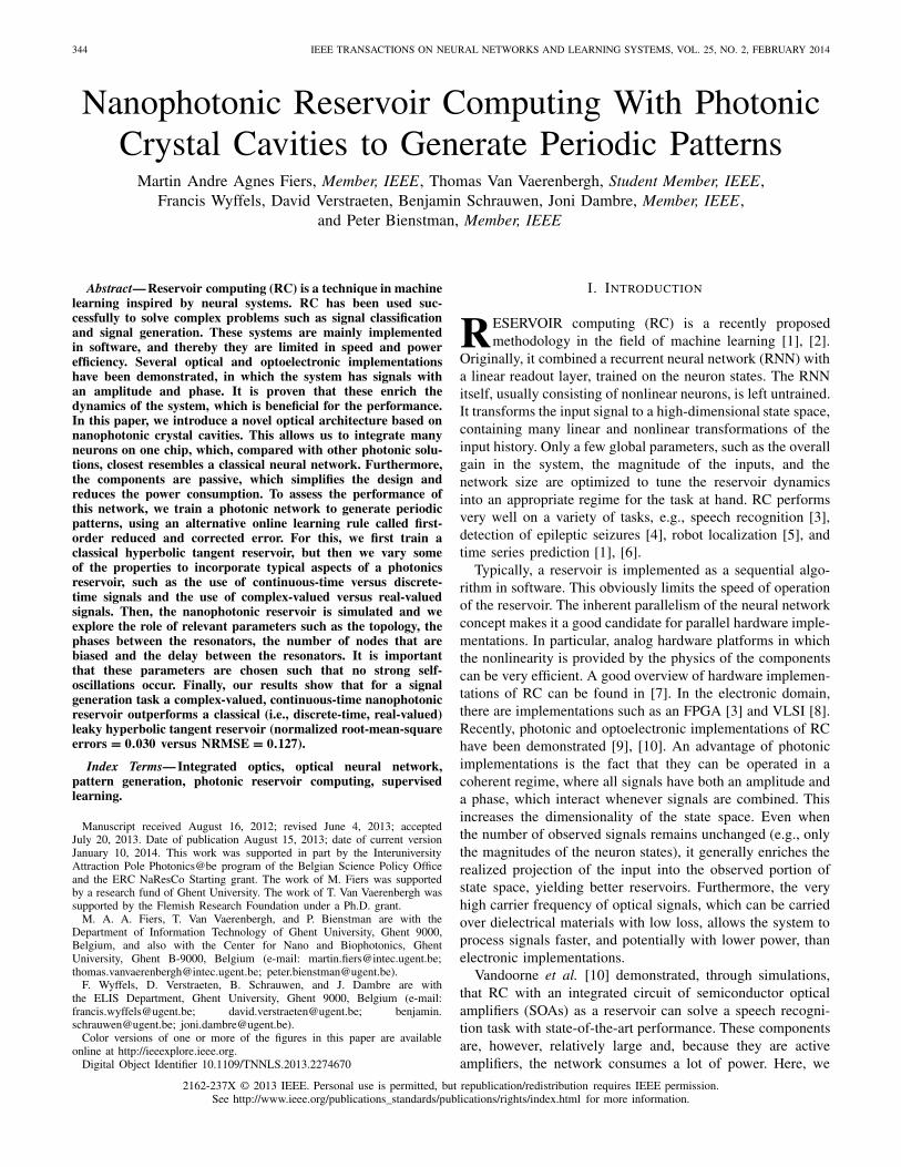
Fig. 1. Reservoir with feedback. The reservoir states x[k] weighted by theoutput weights Wout to produce the output y[k]. This output is then fed backto the input. The purpose of this network is to autonomously generate periodicpatterns after training Wout using the rule described in [12].
The FORCE technique succeeds in training the system withthe actual output feedback in place. The readout weights areadjusted online, e.g., using the recursive least squares (RLS)modification rule. This way, the training considers the reservoirdynamics and dynamic trajectories, including useful basinsof attraction, can be learned. This yields greater robustnessand stability, even when delay is present in the feedbackloop. This is particularly interesting for hardware implemen-tations, as some delay is always present in the physicalsystems.
The steps to perform learning are summarized as follows(Fig. 1).
1) Simulate the reservoir from x[k] to x[k + 1].2) Calculate the output y[k + 1] = Wout[k] x[k + 1].3) Calculate the error with respect to the target signal
f : e[k + 1] = y[k + 1] − s[k + 1].4) From this error, calculate the new weights Wout[k + 1]
using the RLS rule explained in [12].5) Feedback the output y[k + 1] to the reservoir for the
next time step.
FORCE is usually applied to reservoirs, which initiallyexhibit chaotic behavior. For the hyperbolic tangent ESNs, thiscondition is usually met when the spectral radius is consid-erably larger than one. The training stabilizes the dynamicalsystem consisting of the reservoir and the output feedback.
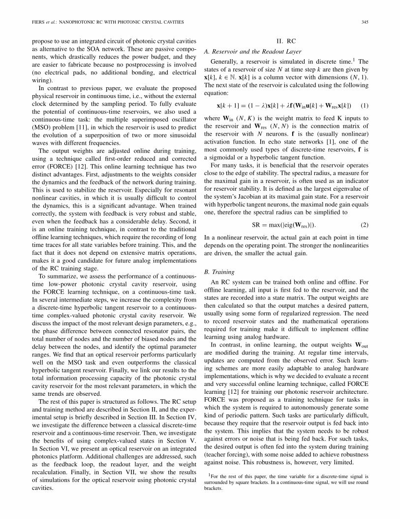
FORCE learning is typically used in a training and eval-uation setup, and is shown in Fig. 2. To be able to scalethis learning approach to periodic signal generation taskswith different time scales, the lengths of all training stagesare expressed as multiples of T1, the period of the slowestfrequency component in the signal that is to be generated.Below, we summarize these steps.
1) Warm-Up (15T1): The initial state x[0] is chosen zero.The input during the warm-up is noise, sampled from astandard normal distribution with amplitude one.
2) Training (400T1): The output weights are adjusted usingthe proposed RLS rule [12].
3) Free-Run (2000T1): The output weights are unmodi-fied. If the training converges, the RC system withfeedback can now autonomously generate the desiredfunction s[k].
Fig. 2. Simplified illustration of the learning sequence. T1 is the periodof the lowest frequency component of the signal that must be generated.During warm-up, the input of the reservoir is noise, sampled from a uniformdistribution. During training, the output weights Wout are adjusted such thatthe output (black solid line) follows the target signal (gray dashed line). Theoutput weights are unmodified during free-run. The output can have a slightlydifferent frequency than the target. The last samples ytest[k] are scrolled over awindow of the free-run output, each time calculating the NRMSE. The optimalvalue of the NRMSE is used as performance for this learning sequence.
III. EXPERIMENTAL SETUP
A. Task Description
As this paper aims to evaluate a photonic reservoirimplementation—inherently operating in continuous time—trained with FORCE learning, we selected the MSO task [11],a pattern generation task defined in continuous time. Thisacademic task has previously been used to benchmark theperformance for the different types of reservoirs. The RCsystem has to generate a superposition of sine waves withharmonically unrelated frequencies
s(t) = sin(ω1t) + sin(ω2t). (3)
The pulsations of the signals are: ω1 = 0.2 /s for the lowerfrequency and ω2 = 0.311 /s for the higher frequency. Whenthis task is used in a discrete-time setup, the target signal issampled at s[k] = s(k�t), k ∈ N. The period of the first signalis T1 = 2π/ω1 � 31.42 s, the period of the second signal isT2 = 2π/ω2 � 20.20. For a classical discrete-time reservoir,�t = 1 s, and we continue using the notation s[k] = s(k ·1 s).The period of the superimposed signal is very long, whichincreases the challenge of learning the signal.
B. Simulation Software
All simulations were performed using a combination oftwo software packages: 1) OGER and 2) Caphe. OGER, theOrGanic Environment for RC [13], extends the Python MDPtoolbox [14], by providing extra functionality in the contextof RC. It is used to setup and postprocess RC experiments andto initiate the reservoir simulations. Caphe [15], a simulationframework for arbitrary nonlinear circuits, is used for theactual continuous-time reservoir simulations.
C. Performance Measure
Reservoir performance is evaluated throughout this paperby the normalized root-mean-square error (NRMSE) betweenthe output and the target function at the sampling times k�t .
FIERS et al.: NANOPHOTONIC RC WITH PHOTONIC CRYSTAL CAVITIES 347
In signal generation tasks, an important aspect of performanceis the stability of the generated output over longer periodsof time. Therefore, after the training phase, we allow thereservoir run for some time (2315T1) before calculating theperformance. In addition, for periodic signals, a small phaseshift between the actual and the desired output is usuallyacceptable, but it strongly affects the NRMSE. We use theapproach of [16], where we calculate the NRMSE for windowsof the output signal ytest[k] = y[2315T1 + k], k ∈ [0, 100T1],and sliding these windows over a sufficiently long section(1000T1) of the free-run stage. Selecting the minimal valueacross all window positions effectively evaluates the shape ofthe desired output, largely cancelling out the impact of anyphase shifts. This is shown in Fig. 2. Although computationallyintensive, this calculation can be sped up using a convolution.
IV. CONTINUOUS-TIME RESERVOIR
The optical network is inherently a continuous-time system,and the MSO task is inherently a continuous-time task, there-fore as an intermediate step toward simulating a full photonicreservoir, we initially investigate the performance of a leakyhyperbolic tangent reservoir as a continuous-time system.
Traditional ESNs are defined in discrete time. We can,however, view the neuron update equation (1) as the resultof applying Euler integration on ordinary differential equa-tions (ODEs). To more closely resemble this form, we nowsubstitute λ by �t/τ0, where τ0 is the dominant time constantof the neuron. In this case, we assume �t = 1 s. To simplifythe notation, we omit the explicit argument of f , and insteadwe write f(v)
x(t + �t) =(
1 − �t1
τ0
)x(t) + �t
1
τ0f(v(t)).
Restructuring and taking the limit for �t → 0 yieldthe equivalent continuous-time leaky hyperbolic tangent ODEequations
d(x)
dt= 1
τ0(−x(t) + f(v(t))). (4)
Note that v(t) also needs to be adapted to explicitly include theinterconnection delays in the network. In a discrete-time RCsystem there is inherently a delay of 1 s between the neurons.To most closely resemble this classical case, all delays are inthis case equal to the original discrete time step of �t = 1 s
v(t) = Winu(t) + Wresx(t − �t).
In a more general setting, a delay on the input connectionscan also be included.
Table I lists the parameters that are used throughout thispaper for the leaky hyperbolic tangent reservoirs. Any devi-ations from these parameters will be explicitly mentioned.We simulate the continuous-time hyperbolic tangent reservoirusing the Bulirsch–Stoer integration method with variablestep size �t ′, and using a relative accuracy of 10−8. Thefeedback is also simulated in continuous time, but withoutdelay. Learning is still performed at discrete time steps of�t = 1 s.
TABLE I
DEFAULT VALUES USED IN THE LEAKY HYPERBOLIC
TANGENT RESERVOIR
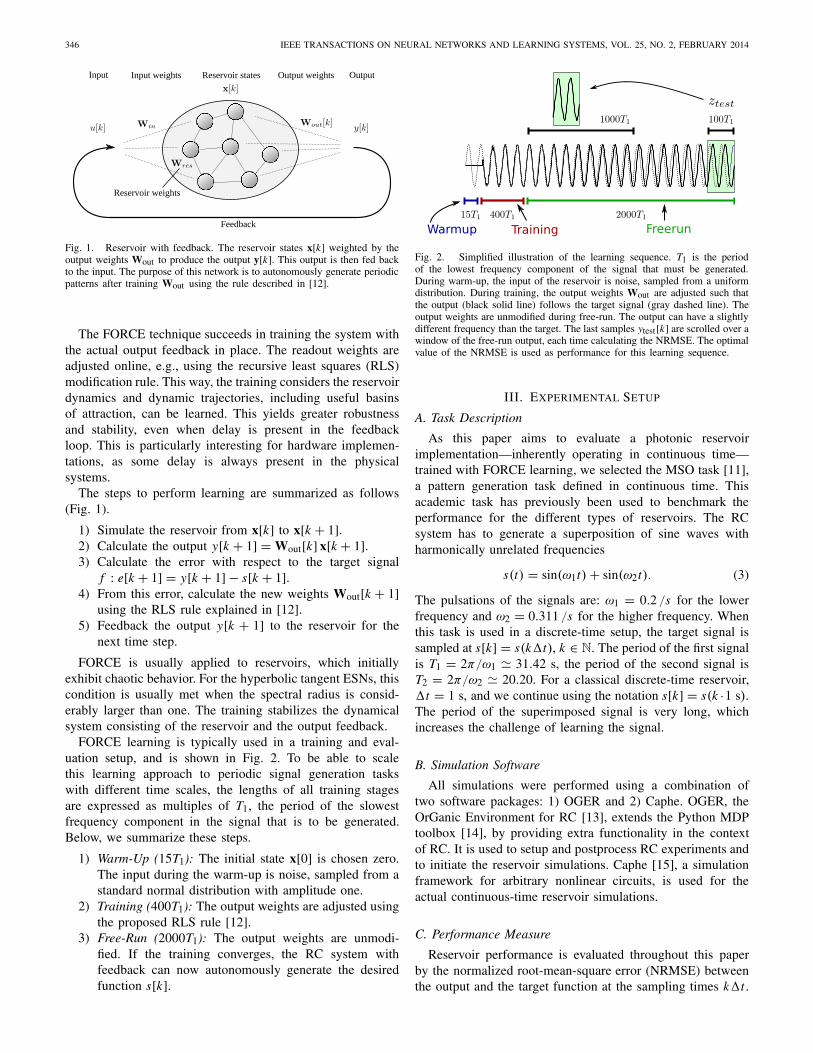
Fig. 3. NRMSE for different τ0 for the MSO task described in Section III-A.The error bars show the sample standard deviation over 40 simulations(NRMSE ± σNRMSE). Solid red line: the error for a standard discrete-timereservoir, often used in the literature and in the practical applications. Dottedgreen line: the performance of a reservoir simulated in continuous time, withcontinuous-time feedback.
We have compared the performance of discrete-time andcontinuous-time reservoirs on the MSO task, as a function ofthe neuron time constant τ0. For each value of τ0 and eachreservoir type, the NRMSE was averaged over 40 experimentswith randomized connection matrix, input noise in the warm-up phase, and input weight matrix. To make a fair comparisonbetween discrete and continuous time, all simulations aresampled at �tsample = 1 s, which means that the trainingstage receives the same number of samples for each reservoir.This also ensures that the learning rate α has the same effectin each case.
The average NRMSE values are summarized in Fig. 3.It shows that moving to continuous time yields a decrease ofthe NRMSE over the full parameter range. This improvementis partly related to the bandwidth: certain frequencies cannotbe captured in discrete time. A continuous-time system intheory has unlimited bandwidth, but for simulations this islimited by the �t ′. Because of the adaptive step-size algorithm,the effective bandwidth varies during the simulation.
For both reservoir types, we can identify an optimal valueof the neuron time constant. For the discrete-time reservoir, wefind an optimal NRMSE of 0.127 at τ0 = 4.0 s, with a samplestandard deviation of 0.111. For the continuous-time reservoir,
348 IEEE TRANSACTIONS ON NEURAL NETWORKS AND LEARNING SYSTEMS, VOL. 25, NO. 2, FEBRUARY 2014
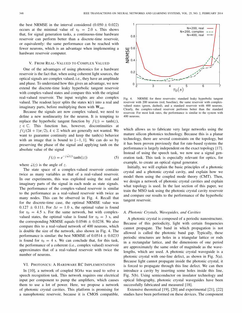
the best NRMSE in the interval considered (0.050 ± 0.022)occurs at the minimal value of τ0 = 2.0 s. This showsthat, for signal generation tasks, a continuous-time hardwarereservoir can perform better than a discrete-time reservoir,or equivalently: the same performance can be reached withfewer neurons, which is an advantage when implementing ahardware reservoir computer.
V. FROM REAL-VALUED TO COMPLEX VALUED
One of the advantages of using photonics for a hardwarereservoir is the fact that, when using coherent light sources, theoptical signals are complex valued, i.e., they have an amplitudeand phase. To understand how this gives an advantage, we nowextend the discrete-time leaky hyperbolic tangent reservoirwith complex-valued states and compare this with the originalreal-valued reservoir. The input weights are also complexvalued. The readout layer splits the states x(t) into a real andimaginary parts, before multiplying them with Wout.
Because the signals are now complex valued, we need todefine a new nonlinearity for the neuron. It is tempting toreplace the hyperbolic tangent function by f (z) = tanh(z),z ∈ C. This function has, however, discontinuities atf ( j (2k + 1)π/2), k ∈ Z which are generally not wanted. Wewant to guarantee continuity and keep the tanh(x) behaviorwith an image that is bound to [−1, 1]. We can do so bypreserving the phase of the signal and applying tanh on theabsolute value of the signal
f (z) = e− j � (z) tanh(|z|) (5)
where � (z) is the angle of z.The state space of a complex-valued reservoir contains
twice as many variables as that of a real-valued reservoir.In our experiments, this was exploited using the real andimaginary parts of the signal in each node as state signals.The performance of the complex-valued reservoir is similarto the performance as a real-valued reservoir with twice asmany nodes. This can be observed in Fig. 4. Recall thatfor the discrete-time case, the optimal NRMSE value was0.127 ± 0.111. For �t = 1.0 s, the optimal value is foundfor τ0 = 4.5 s. For the same network, but with complex-valued states, the optimal value is found for τ0 = 3 s, andthe corresponding NRMSE equals 0.0546 ± 0.0238. We alsocompare this to a real-valued network of 400 neurons, whichis double the size of the network, also shown in Fig. 4. Theperformance is similar: the best NRMSE of 0.0514 ± 0.0233is found for τ0 = 4 s. We can conclude that, for this task,the performance of a coherent (i.e., complex valued) reservoirapproximates that of a real-valued reservoir with twice thenumber of neurons.
VI. PHOTONICS: A HARDWARE RC IMPLEMENTATION
In [10], a network of coupled SOAs was used to solve aspeech recognition task. This network requires one electricalinput per component to pump the amplifiers, which causesthem to use a lot of power. Here, we propose a networkof photonic crystal cavities. This platform is promising fora nanophotonic reservoir, because it is CMOS compatible,
Fig. 4. NRMSE for three reservoirs: standard leaky hyperbolic tangentreservoir with 200 neurons (red, baseline), the same reservoir with complex-valued states (green, dashed), and a standard reservoir with 400 neurons.Clearly, the complex-valued reservoir performs better than the standardreservoir. For most leak rates, the performance is similar to the system with400 neurons.
which allows us to fabricate very large networks using themature silicon photonics technology. Because this is a planartechnology, there are several constraints on the topology, butit has been proven previously that for rate-based systems theperformance is largely independent on the exact topology [17].Instead of using the speech task, we now use a signal gen-eration task. This task is especially relevant for optics, forexample, to create an optical signal generator.
Initially, we will explain the basic principles of a photoniccrystal and a photonic crystal cavity, and explain how wemodel them using the coupled mode theory (CMT). Then,we design a network of photonic crystal cavities and explainwhat topology is used. In the last section of this paper, wetrain the MSO task using the photonic crystal cavity reservoirand compare our results to the performance of the hyperbolictangent reservoir.
A. Photonic Crystals, Waveguides, and Cavities
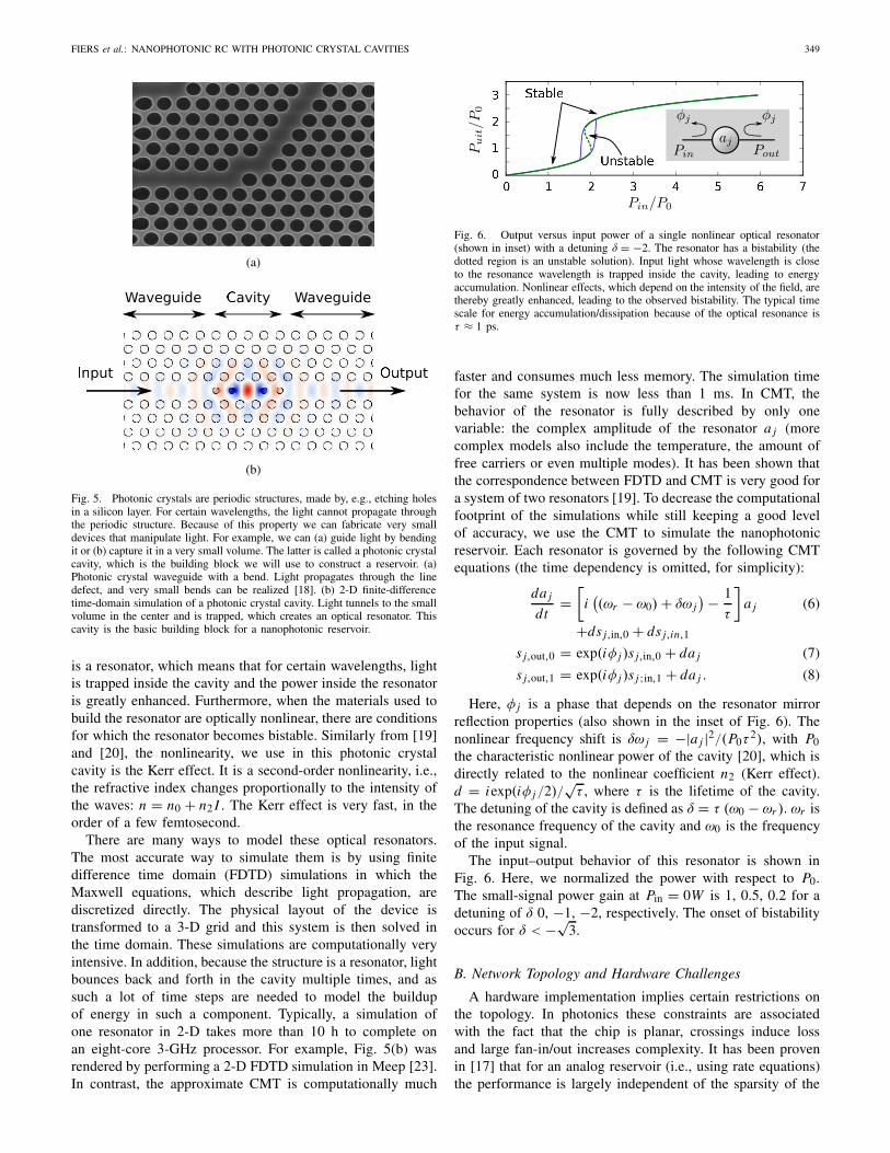
A photonic crystal is composed of a periodic nanostructure.Because of this periodicity, light with certain frequenciescannot propagate. The band in which propagation is notallowed is called the photonic band gap. Typically, theseperiodic structures are holes in a triangular lattice or rodsin a rectangular lattice, and the dimensions of one periodare approximately the same order of magnitude as the wave-lengths, which are used. A photonic crystal waveguide is aphotonic crystal with one-line defect, as shown in Fig. 5(a).Because light cannot propagate inside the photonic crystal, itis forced to propagate through this line defect. We can thenintroduce a cavity by inserting some holes inside this line,Fig. 5(b). Using semiconductor on insulator technology andoptical lithography, photonic crystal waveguides have beensuccessfully fabricated and measured [18].
Extensive theoretical [19], [20] and experimental [21], [22]studies have been performed on these devices. The component
FIERS et al.: NANOPHOTONIC RC WITH PHOTONIC CRYSTAL CAVITIES 349
Fig. 5. Photonic crystals are periodic structures, made by, e.g., etching holesin a silicon layer. For certain wavelengths, the light cannot propagate throughthe periodic structure. Because of this property we can fabricate very smalldevices that manipulate light. For example, we can (a) guide light by bendingit or (b) capture it in a very small volume. The latter is called a photonic crystalcavity, which is the building block we will use to construct a reservoir. (a)Photonic crystal waveguide with a bend. Light propagates through the linedefect, and very small bends can be realized [18]. (b) 2-D finite-differencetime-domain simulation of a photonic crystal cavity. Light tunnels to the smallvolume in the center and is trapped, which creates an optical resonator. Thiscavity is the basic building block for a nanophotonic reservoir.
is a resonator, which means that for certain wavelengths, lightis trapped inside the cavity and the power inside the resonatoris greatly enhanced. Furthermore, when the materials used tobuild the resonator are optically nonlinear, there are conditionsfor which the resonator becomes bistable. Similarly from [19]and [20], the nonlinearity, we use in this photonic crystalcavity is the Kerr effect. It is a second-order nonlinearity, i.e.,the refractive index changes proportionally to the intensity ofthe waves: n = n0 + n2 I . The Kerr effect is very fast, in theorder of a few femtosecond.
There are many ways to model these optical resonators.The most accurate way to simulate them is by using finitedifference time domain (FDTD) simulations in which theMaxwell equations, which describe light propagation, arediscretized directly. The physical layout of the device istransformed to a 3-D grid and this system is then solved inthe time domain. These simulations are computationally veryintensive. In addition, because the structure is a resonator, lightbounces back and forth in the cavity multiple times, and assuch a lot of time steps are needed to model the buildupof energy in such a component. Typically, a simulation ofone resonator in 2-D takes more than 10 h to complete onan eight-core 3-GHz processor. For example, Fig. 5(b) wasrendered by performing a 2-D FDTD simulation in Meep [23].In contrast, the approximate CMT is computationally much
Fig. 6. Output versus input power of a single nonlinear optical resonator(shown in inset) with a detuning δ = −2. The resonator has a bistability (thedotted region is an unstable solution). Input light whose wavelength is closeto the resonance wavelength is trapped inside the cavity, leading to energyaccumulation. Nonlinear effects, which depend on the intensity of the field, arethereby greatly enhanced, leading to the observed bistability. The typical timescale for energy accumulation/dissipation because of the optical resonance isτ ≈ 1 ps.
faster and consumes much less memory. The simulation timefor the same system is now less than 1 ms. In CMT, thebehavior of the resonator is fully described by only onevariable: the complex amplitude of the resonator a j (morecomplex models also include the temperature, the amount offree carriers or even multiple modes). It has been shown thatthe correspondence between FDTD and CMT is very good fora system of two resonators [19]. To decrease the computationalfootprint of the simulations while still keeping a good levelof accuracy, we use the CMT to simulate the nanophotonicreservoir. Each resonator is governed by the following CMTequations (the time dependency is omitted, for simplicity):
da j
dt=
[i((ωr − ω0) + δω j
) − 1
τ
]a j (6)
+ds j,in,0 + ds j,in,1
s j,out,0 = exp(iφ j )s j,in,0 + da j (7)
s j,out,1 = exp(iφ j )s j ;in,1 + da j . (8)
Here, φ j is a phase that depends on the resonator mirrorreflection properties (also shown in the inset of Fig. 6). Thenonlinear frequency shift is δω j = −|a j |2/(P0τ
2), with P0the characteristic nonlinear power of the cavity [20], which isdirectly related to the nonlinear coefficient n2 (Kerr effect).d = iexp(iφ j/2)/
√τ , where τ is the lifetime of the cavity.
The detuning of the cavity is defined as δ = τ (ω0 − ωr ). ωr isthe resonance frequency of the cavity and ω0 is the frequencyof the input signal.
The input–output behavior of this resonator is shown inFig. 6. Here, we normalized the power with respect to P0.The small-signal power gain at Pin = 0W is 1, 0.5, 0.2 for adetuning of δ 0, −1, −2, respectively. The onset of bistabilityoccurs for δ < −√
3.
B. Network Topology and Hardware Challenges
A hardware implementation implies certain restrictions onthe topology. In photonics these constraints are associatedwith the fact that the chip is planar, crossings induce lossand large fan-in/out increases complexity. It has been provenin [17] that for an analog reservoir (i.e., using rate equations)the performance is largely independent of the sparsity of the
350 IEEE TRANSACTIONS ON NEURAL NETWORKS AND LEARNING SYSTEMS, VOL. 25, NO. 2, FEBRUARY 2014
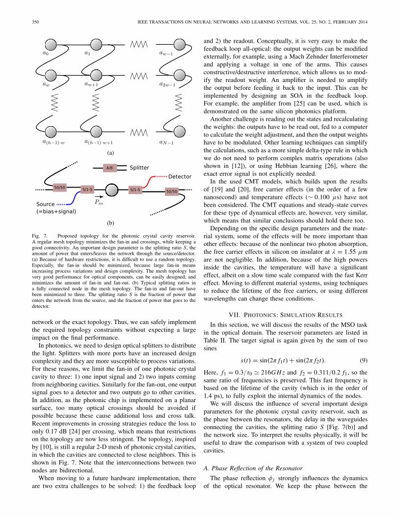
Fig. 7. Proposed topology for the photonic crystal cavity reservoir.A regular mesh topology minimizes the fan-in and crossings, while keeping agood connectivity. An important design parameter is the splitting ratio S, theamount of power that enters/leaves the network through the source/detector.(a) Because of hardware restrictions, it is difficult to use a random topology.Especially, the fan-in should be minimized, because large fan-in meansincreasing process variations and design complexity. The mesh topology hasvery good performance for optical components, can be easily designed, andminimizes the amount of fan-in and fan-out. (b) Typical splitting ratios ina fully connected node in the mesh topology. The fan-in and fan-out havebeen minimized to three. The splitting ratio S is the fraction of power thatenters the network from the source, and the fraction of power that goes to thedetector.
network or the exact topology. Thus, we can safely implementthe required topology constraints without expecting a largeimpact on the final performance.
In photonics, we need to design optical splitters to distributethe light. Splitters with more ports have an increased designcomplexity and they are more susceptible to process variations.For these reasons, we limit the fan-in of one photonic crystalcavity to three: 1) one input signal and 2) two inputs comingfrom neighboring cavities. Similarly for the fan-out, one outputsignal goes to a detector and two outputs go to other cavities.In addition, as the photonic chip is implemented on a planarsurface, too many optical crossings should be avoided ifpossible because these cause additional loss and cross talk.Recent improvements in crossing strategies reduce the loss toonly 0.17 dB [24] per crossing, which means that restrictionson the topology are now less stringent. The topology, inspiredby [10], is still a regular 2-D mesh of photonic crystal cavities,in which the cavities are connected to close neighbors. This isshown in Fig. 7. Note that the interconnections between twonodes are bidirectional.
When moving to a future hardware implementation, thereare two extra challenges to be solved: 1) the feedback loop
and 2) the readout. Conceptually, it is very easy to make thefeedback loop all-optical: the output weights can be modifiedexternally, for example, using a Mach Zehnder Interferometerand applying a voltage in one of the arms. This causesconstructive/destructive interference, which allows us to mod-ify the readout weight. An amplifier is needed to amplifythe output before feeding it back to the input. This can beimplemented by designing an SOA in the feedback loop.For example, the amplifier from [25] can be used, which isdemonstrated on the same silicon photonics platform.
Another challenge is reading out the states and recalculatingthe weights: the outputs have to be read out, fed to a computerto calculate the weight adjustment, and then the output weightshave to be modulated. Other learning techniques can simplifythe calculations, such as a more simple delta-type rule in whichwe do not need to perform complex matrix operations (alsoshown in [12]), or using Hebbian learning [26], where theexact error signal is not explicitly needed.
In the used CMT models, which builds upon the resultsof [19] and [20], free carrier effects (in the order of a fewnanosecond) and temperature effects (∼ 0.100 μs) have notbeen considered. The CMT equations and steady-state curvesfor these type of dynamical effects are, however, very similar,which means that similar conclusions should hold there too.
Depending on the specific design parameters and the mate-rial system, some of the effects will be more important thanother effects: because of the nonlinear two photon absorption,the free carrier effects in silicon on insulator at λ = 1.55 μmare not negligible. In addition, because of the high powersinside the cavities, the temperature will have a significanteffect, albeit on a slow time scale compared with the fast Kerreffect. Moving to different material systems, using techniquesto reduce the lifetime of the free carriers, or using differentwavelengths can change these conditions.
VII. PHOTONICS: SIMULATION RESULTS
In this section, we will discuss the results of the MSO taskin the optical domain. The reservoir parameters are listed inTable II. The target signal is again given by the sum of twosines
s(t) = sin(2π f1t) + sin(2π f2t). (9)
Here, f1 = 0.3/τ0 � 216G H z and f2 = 0.311/0.2 f1, so thesame ratio of frequencies is preserved. This fast frequency isbased on the lifetime of the cavity (which is in the order of1.4 ps), to fully exploit the internal dynamics of the nodes.
We will discuss the influence of several important designparameters for the photonic crystal cavity reservoir, such asthe phase between the resonators, the delay in the waveguidesconnecting the cavities, the splitting ratio S [Fig. 7(b)] andthe network size. To interpret the results physically, it will beuseful to draw the comparison with a system of two coupledcavities.
A. Phase Reflection of the Resonator
The phase reflection φ j strongly influences the dynamicsof the optical resonator. We keep the phase between the
FIERS et al.: NANOPHOTONIC RC WITH PHOTONIC CRYSTAL CAVITIES 351
TABLE II
DEFAULT VALUES USED IN THE PHOTONIC CRYSTAL CAVITY RESERVOIR
resonators (which is determined by the waveguide between theresonators) fixed, which is a realistic assumption if engineeredcorrectly.
For a dynamical system, a linear stability analysis revealswhether the system is stable or not. This is done by examiningthe eigenvalues of the Jacobian of the system. If all eigenvalueshave a negative real part, the system is stable. In somecases, an unstable fixed point implies chaos or self-pulsation.To distinguish between both, we can calculate the maximalLyapunov exponent of the system. If the maximal Lyapunovexponent is larger than zero, the system is chaotic. For a stableperiodic solution, the maximal Lyapunov exponent is zero.
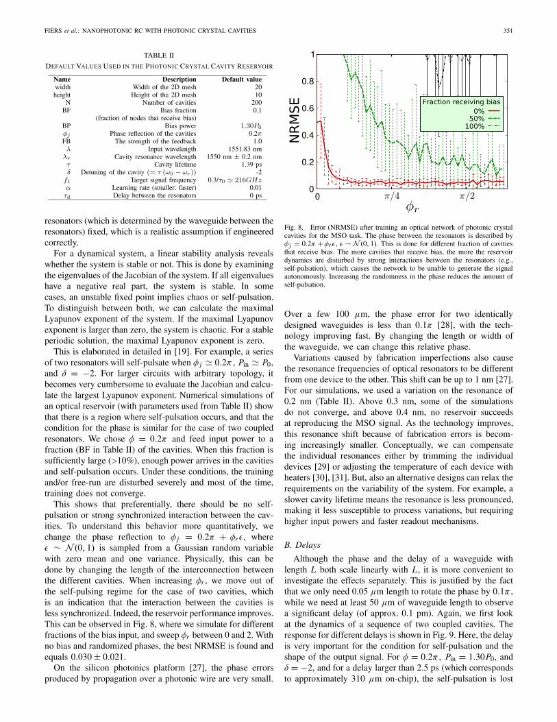
This is elaborated in detailed in [19]. For example, a seriesof two resonators will self-pulsate when φ j � 0.2π , Pin � P0,and δ = −2. For larger circuits with arbitrary topology, itbecomes very cumbersome to evaluate the Jacobian and calcu-late the largest Lyapunov exponent. Numerical simulations ofan optical reservoir (with parameters used from Table II) showthat there is a region where self-pulsation occurs, and that thecondition for the phase is similar for the case of two coupledresonators. We chose φ = 0.2π and feed input power to afraction (BF in Table II) of the cavities. When this fraction issufficiently large (>10%), enough power arrives in the cavitiesand self-pulsation occurs. Under these conditions, the trainingand/or free-run are disturbed severely and most of the time,training does not converge.
This shows that preferentially, there should be no self-pulsation or strong synchronized interaction between the cav-ities. To understand this behavior more quantitatively, wechange the phase reflection to φ j = 0.2π + φrε, whereε ∼ N (0, 1) is sampled from a Gaussian random variablewith zero mean and one variance. Physically, this can bedone by changing the length of the interconnection betweenthe different cavities. When increasing φr , we move out ofthe self-pulsing regime for the case of two cavities, whichis an indication that the interaction between the cavities isless synchronized. Indeed, the reservoir performance improves.This can be observed in Fig. 8, where we simulate for differentfractions of the bias input, and sweep φr between 0 and 2. Withno bias and randomized phases, the best NRMSE is found andequals 0.030 ± 0.021.
On the silicon photonics platform [27], the phase errorsproduced by propagation over a photonic wire are very small.
Fig. 8. Error (NRMSE) after training an optical network of photonic crystalcavities for the MSO task. The phase between the resonators is described byφ j = 0.2π +φr ε, ε ∼ N (0, 1). This is done for different fraction of cavitiesthat receive bias. The more cavities that receive bias, the more the reservoirdynamics are disturbed by strong interactions between the resonators (e.g.,self-pulsation), which causes the network to be unable to generate the signalautonomously. Increasing the randomness in the phase reduces the amount ofself-pulsation.
Over a few 100 μm, the phase error for two identicallydesigned waveguides is less than 0.1π [28], with the tech-nology improving fast. By changing the length or width ofthe waveguide, we can change this relative phase.
Variations caused by fabrication imperfections also causethe resonance frequencies of optical resonators to be differentfrom one device to the other. This shift can be up to 1 nm [27].For our simulations, we used a variation on the resonance of0.2 nm (Table II). Above 0.3 nm, some of the simulationsdo not converge, and above 0.4 nm, no reservoir succeedsat reproducing the MSO signal. As the technology improves,this resonance shift because of fabrication errors is becom-ing increasingly smaller. Conceptually, we can compensatethe individual resonances either by trimming the individualdevices [29] or adjusting the temperature of each device withheaters [30], [31]. But, also an alternative designs can relax therequirements on the variability of the system. For example, aslower cavity lifetime means the resonance is less pronounced,making it less susceptible to process variations, but requiringhigher input powers and faster readout mechanisms.
B. Delays
Although the phase and the delay of a waveguide withlength L both scale linearly with L, it is more convenient toinvestigate the effects separately. This is justified by the factthat we only need 0.05 μm length to rotate the phase by 0.1π ,while we need at least 50 μm of waveguide length to observea significant delay (of approx. 0.1 pm). Again, we first lookat the dynamics of a sequence of two coupled cavities. Theresponse for different delays is shown in Fig. 9. Here, the delayis very important for the condition for self-pulsation and theshape of the output signal. For φ = 0.2π , Pin = 1.30P0, andδ = −2, and for a delay larger than 2.5 ps (which correspondsto approximately 310 μm on-chip), the self-pulsation is lost
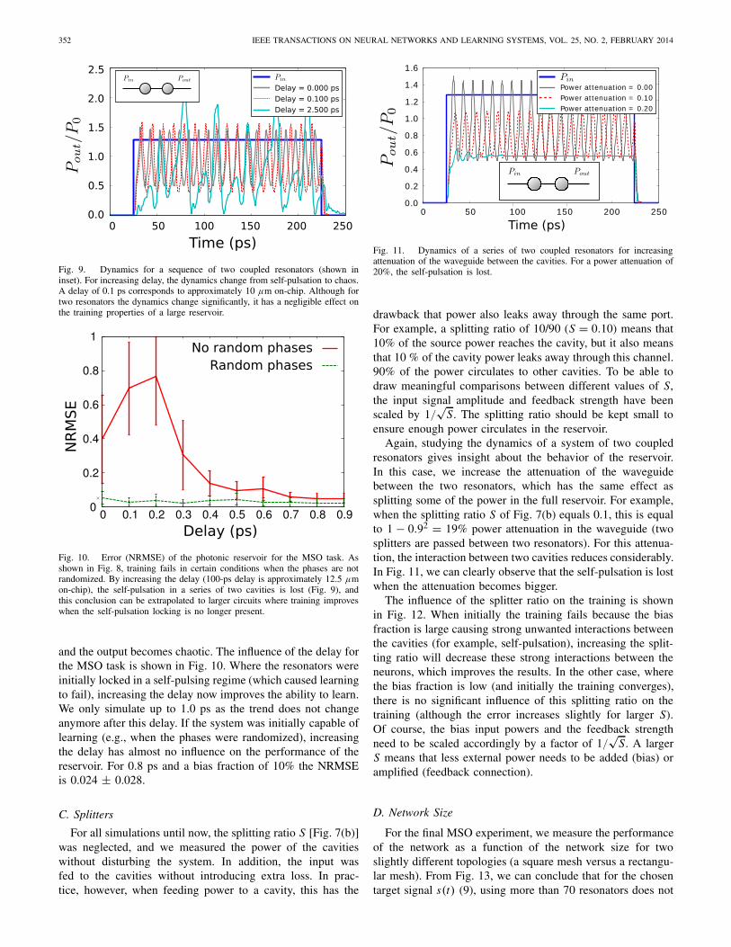
352 IEEE TRANSACTIONS ON NEURAL NETWORKS AND LEARNING SYSTEMS, VOL. 25, NO. 2, FEBRUARY 2014
Fig. 9. Dynamics for a sequence of two coupled resonators (shown ininset). For increasing delay, the dynamics change from self-pulsation to chaos.A delay of 0.1 ps corresponds to approximately 10 μm on-chip. Although fortwo resonators the dynamics change significantly, it has a negligible effect onthe training properties of a large reservoir.
Fig. 10. Error (NRMSE) of the photonic reservoir for the MSO task. Asshown in Fig. 8, training fails in certain conditions when the phases are notrandomized. By increasing the delay (100-ps delay is approximately 12.5 μmon-chip), the self-pulsation in a series of two cavities is lost (Fig. 9), andthis conclusion can be extrapolated to larger circuits where training improveswhen the self-pulsation locking is no longer present.
and the output becomes chaotic. The influence of the delay forthe MSO task is shown in Fig. 10. Where the resonators wereinitially locked in a self-pulsing regime (which caused learningto fail), increasing the delay now improves the ability to learn.We only simulate up to 1.0 ps as the trend does not changeanymore after this delay. If the system was initially capable oflearning (e.g., when the phases were randomized), increasingthe delay has almost no influence on the performance of thereservoir. For 0.8 ps and a bias fraction of 10% the NRMSEis 0.024 ± 0.028.
C. Splitters
For all simulations until now, the splitting ratio S [Fig. 7(b)]was neglected, and we measured the power of the cavitieswithout disturbing the system. In addition, the input wasfed to the cavities without introducing extra loss. In prac-tice, however, when feeding power to a cavity, this has the
Fig. 11. Dynamics of a series of two coupled resonators for increasingattenuation of the waveguide between the cavities. For a power attenuation of20%, the self-pulsation is lost.
drawback that power also leaks away through the same port.For example, a splitting ratio of 10/90 (S = 0.10) means that10% of the source power reaches the cavity, but it also meansthat 10 % of the cavity power leaks away through this channel.90% of the power circulates to other cavities. To be able todraw meaningful comparisons between different values of S,the input signal amplitude and feedback strength have beenscaled by 1/
√S. The splitting ratio should be kept small to
ensure enough power circulates in the reservoir.Again, studying the dynamics of a system of two coupled
resonators gives insight about the behavior of the reservoir.In this case, we increase the attenuation of the waveguidebetween the two resonators, which has the same effect assplitting some of the power in the full reservoir. For example,when the splitting ratio S of Fig. 7(b) equals 0.1, this is equalto 1 − 0.92 = 19% power attenuation in the waveguide (twosplitters are passed between two resonators). For this attenua-tion, the interaction between two cavities reduces considerably.In Fig. 11, we can clearly observe that the self-pulsation is lostwhen the attenuation becomes bigger.
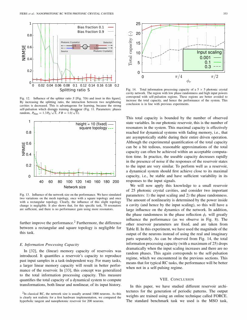
The influence of the splitter ratio on the training is shownin Fig. 12. When initially the training fails because the biasfraction is large causing strong unwanted interactions betweenthe cavities (for example, self-pulsation), increasing the split-ting ratio will decrease these strong interactions between theneurons, which improves the results. In the other case, wherethe bias fraction is low (and initially the training converges),there is no significant influence of this splitting ratio on thetraining (although the error increases slightly for larger S).Of course, the bias input powers and the feedback strengthneed to be scaled accordingly by a factor of 1/
√S. A larger
S means that less external power needs to be added (bias) oramplified (feedback connection).
D. Network Size
For the final MSO experiment, we measure the performanceof the network as a function of the network size for twoslightly different topologies (a square mesh versus a rectangu-lar mesh). From Fig. 13, we can conclude that for the chosentarget signal s(t) (9), using more than 70 resonators does not
FIERS et al.: NANOPHOTONIC RC WITH PHOTONIC CRYSTAL CAVITIES 353
Fig. 12. Influence of the splitter ratio S [Fig. 7(b) and inset in this figure].By increasing the splitting ratio, the interaction between two neighboringcavities is decreased. This is advantageous for learning, because the strongself-pulsation which disrupts training disappear (Fig. 11. Parameters: phasesrandom, Pbias = 1.3P0/
√S, F B = 1.0/
√S).
Fig. 13. Influence of the network size on the performance. We have simulatedtwo variations on the mesh topology, once with a square topology and oncewith a rectangular topology. Clearly, the influence of this slight topologychange is negligible. It also shows that, for this specific task, 70 resonatorsare sufficient, and there is no performance gain using more resonators.
further improve the performance.2 Furthermore, the differencebetween a rectangular and square topology is negligible forthis task.
E. Information Processing Capacity
In [32], the (linear) memory capacity of reservoirs wasintroduced. It quantifies a reservoir’s capacity to reproducepast input samples in a task-independent way. For many tasks,a larger linear memory capacity will result in better perfor-mance of the reservoir. In [33], this concept was generalizedto the total information processing capacity. This measurequantifies the total capacity of a dynamical system to computetransformations, both linear and nonlinear, of its input history.
2In classical RC, the network size is usually around 1000 neurons. As thisis clearly not realistic for a first hardware implementation, we compared thehyperbolic tangent and nanophotonic reservoir for 200 neurons.
Fig. 14. Total information processing capacity of a 5 × 5 photonic crystalcavity network. The region with low phase randomness and high input powerscorrespond with self-pulsation regions. These regions are better avoided toincrease the total capacity, and hence the performance of the system. Thisconclusion is in line with previous experiments.
This total capacity is bounded by the number of observedstate variables. In our photonic reservoir, this is the number ofresonators in the system. This maximal capacity is effectivelyreached for dynamical systems with fading memory, i.e., thatare asymptotically stable during their entire driven operation.Although the experimental quantification of the total capacitycan be a bit tedious, reasonable approximations of the totalcapacity can often be achieved within an acceptable computa-tion time. In practice, the useable capacity decreases rapidlyin the presence of noise if the responses of the reservoir statesto the input are very similar. To perform well as a reservoir,a dynamical system should first achieve close to its maximalcapacity, i.e., be stable and have sufficient variability in itsresponses to the input signals.
We will now apply this knowledge to a small reservoirof 25 photonic crystal cavities, and consider two importantparameters: 1) the input scaling and 2) the phase randomness.The amount of nonlinearity is determined by the power insidea cavity (and hence by the input scaling), so this will have alarge influence on the dynamics of the network. In addition,the phase randomness in the phase reflection φr will greatlyinfluence the performance (as we observe in Fig. 8). Theother reservoir parameters are fixed, and are taken fromTable II. In this experiment, we have used the magnitude of theoutput of the neurons instead of using the real and imaginaryparts separately. As can be observed from Fig. 14, the totalinformation processing capacity (with a maximum of 25) dropsdramatically when the input scaling increases and there are norandom phases. This again corresponds to the self-pulsationregime, which we encountered in the previous sections. Thismeans that for typical RC tasks, the performance will be betterwhen not in a self-pulsing regime.
VIII. CONCLUSION
In this paper, we have studied different reservoir archi-tectures for the generation of periodic patterns. The outputweights are trained using an online technique called FORCE.The standard benchmark task we used is the MSO task,
354 IEEE TRANSACTIONS ON NEURAL NETWORKS AND LEARNING SYSTEMS, VOL. 25, NO. 2, FEBRUARY 2014
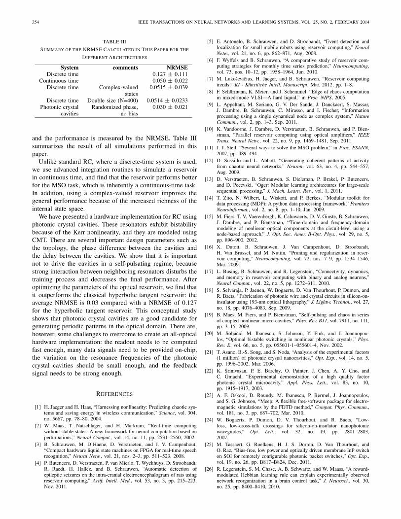
TABLE III
SUMMARY OF THE NRMSE CALCULATED IN THIS PAPER FOR THE
DIFFERENT ARCHITECTURES
and the performance is measured by the NRMSE. Table IIIsummarizes the result of all simulations performed in thispaper.
Unlike standard RC, where a discrete-time system is used,we use advanced integration routines to simulate a reservoirin continuous time, and find that the reservoir performs betterfor the MSO task, which is inherently a continuous-time task.In addition, using a complex-valued reservoir improves thegeneral performance because of the increased richness of theinternal state space.
We have presented a hardware implementation for RC usingphotonic crystal cavities. These resonators exhibit bistabilitybecause of the Kerr nonlinearity, and they are modeled usingCMT. There are several important design parameters such asthe topology, the phase difference between the cavities andthe delay between the cavities. We show that it is importantnot to drive the cavities in a self-pulsating regime, becausestrong interaction between neighboring resonators disturbs thetraining process and decreases the final performance. Afteroptimizing the parameters of the optical reservoir, we find thatit outperforms the classical hyperbolic tangent reservoir: theaverage NRMSE is 0.03 compared with a NRMSE of 0.127for the hyperbolic tangent reservoir. This conceptual studyshows that photonic crystal cavities are a good candidate forgenerating periodic patterns in the optical domain. There are,however, some challenges to overcome to create an all-opticalhardware implementation: the readout needs to be computedfast enough, many data signals need to be provided on-chip,the variation on the resonance frequencies of the photoniccrystal cavities should be small enough, and the feedbacksignal needs to be strong enough.
REFERENCES
[1] H. Jaeger and H. Haas, “Harnessing nonlinearity: Predicting chaotic sys-tems and saving energy in wireless communication,” Science, vol. 304,no. 5667, pp. 78–80, 2004.
[2] W. Maas, T. Natschlager, and H. Markram, “Real-time computingwithout stable states: A new framework for neural computation based onperturbations,” Neural Comput., vol. 14, no. 11, pp. 2531–2560, 2002.
[3] B. Schrauwen, M. D’Haene, D. Verstraeten, and J. V. Campenhout,“Compact hardware liquid state machines on FPGA for real-time speechrecognition,” Neural Netw., vol. 21, nos. 2–3, pp. 511–523, 2008.
[4] P. Buteneers, D. Verstraeten, P. van Mierlo, T. Wyckhuys, D. Stroobandt,R. Raedt, H. Hallez, and B. Schrauwen, “Automatic detection ofepileptic seizures on the intra-cranial electroencephalogram of rats usingreservoir computing,” Artif. Intell. Med., vol. 53, no. 3, pp. 215–223,Nov. 2011.
[5] E. Antonelo, B. Schrauwen, and D. Stroobandt, “Event detection andlocalization for small mobile robots using reservoir computing,” NeuralNetw., vol. 21, no. 6, pp. 862–871, Aug. 2008.
[6] F. Wyffels and B. Schrauwen, “A comparative study of reservoir com-puting strategies for monthly time series prediction,” Neurocomputing,vol. 73, nos. 10–12, pp. 1958–1964, Jun. 2010.
[7] M. Lukoševicius, H. Jaeger, and B. Schrauwen, “Reservoir computingtrends,” KI - Künstliche Intell. Manuscript, Mar. 2012, pp. 1–8.
[8] F. Schürmann, K. Meier, and J. Schemmel, “Edge of chaos computationin mixed-mode VLSI—A hard liquid,” in Proc. NIPS, 2005.
[9] L. Appeltant, M. Soriano, G. V. Der Sande, J. Danckaert, S. Massar,J. Dambre, B. Schrauwen, C. Mirasso, and I. Fischer, “Informationprocessing using a single dynamical node as complex system,” NatureCommun., vol. 2, pp. 1–3, Sep. 2011.
[10] K. Vandoorne, J. Dambre, D. Verstraeten, B. Schrauwen, and P. Bien-stman, “Parallel reservoir computing using optical amplifiers,” IEEETrans. Neural Netw., vol. 22, no. 9, pp. 1469–1481, Sep. 2011.
[11] J. J. Steil, “Several ways to solve the MSO problem,” in Proc. ESANN,2007, pp. 489–494.
[12] D. Sussillo and L. Abbott, “Generating coherent patterns of activityfrom chaotic neural networks,” Neuron, vol. 63, no. 4, pp. 544–557,Aug. 2009.
[13] D. Verstraeten, B. Schrauwen, S. Dieleman, P. Brakel, P. Buteneers,and D. Pecevski, “Oger: Modular learning architectures for large-scalesequential processing,” J. Mach. Learn. Res., vol. 1, 2011.
[14] T. Zito, N. Wilbert, L. Wiskott, and P. Berkes, “Modular toolkit fordata processing (MDP): A python data processing framework,” FrontiersNeuroinformat., vol. 2, no. 8, pp. 1–10, Jan. 2009.
[15] M. Fiers, T. V. Vaerenbergh, K. Caluwaerts, D. V. Ginste, B. Schrauwen,J. Dambre, and P. Bienstman, “Time-domain and frequency-domainmodeling of nonlinear optical components at the circuit-level using anode-based approach,” J. Opt. Soc. Amer. B-Opt. Phys., vol. 29, no. 5,pp. 896–900, 2012.
[16] X. Dutoit, B. Schrauwen, J. Van Campenhout, D. Stroobandt,H. Van Brussel, and M. Nuttin, “Pruning and regularization in reser-voir computing,” Neurocomputing, vol. 72, nos. 7–9, pp. 1534–1546,Mar. 2009.
[17] L. Busing, B. Schrauwen, and R. Legenstein, “Connectivity, dynamics,and memory in reservoir computing with binary and analog neurons,”Neural Comput., vol. 22, no. 5, pp. 1272–311, 2010.
[18] S. Selvaraja, P. Jaenen, W. Bogaerts, D. Van Thourhout, P. Dumon, andR. Baets, “Fabrication of photonic wire and crystal circuits in silicon-on-insulator using 193-nm optical lithography,” J. Lightw. Technol., vol. 27,no. 18, pp. 4076–4083, Sep. 2009.
[19] B. Maes, M. Fiers, and P. Bienstman, “Self-pulsing and chaos in seriesof coupled nonlinear micro-cavities,” Phys. Rev. B11, vol. 7911, no. 111,pp. 3–15, 2009.
[20] M. Soljacic, M. Ibanescu, S. Johnson, Y. Fink, and J. Joannopou-los, “Optimal bistable switching in nonlinear photonic crystals,” Phys.Rev. E, vol. 66, no. 5, pp. 055601-1–055601-4, Nov. 2002.
[21] T. Asano, B.-S. Song, and S. Noda, “Analysis of the experimental factors(1 million) of photonic crystal nanocavities,” Opt. Exp., vol. 14, no. 5,pp. 1996–2002, Mar. 2006.
[22] K. Srinivasan, P. E. Barclay, O. Painter, J. Chen, A. Y. Cho, andC. Gmachl, “Experimental demonstration of a high quality factorphotonic crystal microcavity,” Appl. Phys. Lett., vol. 83, no. 10,pp. 1915–1917, 2003.
[23] A. F. Oskooi, D. Roundy, M. Ibanescu, P. Bermel, J. Joannopoulos,and S. G. Johnson, “Meep: A flexible free-software package for electro-magnetic simulations by the FDTD method,” Comput. Phys. Commun.,vol. 181, no. 3, pp. 687–702, Mar. 2010.
[24] W. Bogaerts, P. Dumon, D. V. Thourhout, and R. Baets, “Low-loss, low-cross-talk crossings for silicon-on-insulator nanophotonicwaveguides,” Opt. Lett., vol. 32, no. 19, pp. 2801–2803,2007.
[25] M. Tassaert, G. Roelkens, H. J. S. Dorren, D. Van Thourhout, andO. Raz, “Bias-free, low power and optically driven membrane InP switchon SOI for remotely configurable photonic packet switches,” Opt. Exp.,vol. 19, no. 26, pp. B817–B824, Dec. 2011.
[26] R. Legenstein, S. M. Chase, A. B. Schwartz, and W. Maass, “A reward-modulated Hebbian learning rule can explain experimentally observednetwork reorganization in a brain control task,” J. Neurosci., vol. 30,no. 25, pp. 8400–8410, 2010.
FIERS et al.: NANOPHOTONIC RC WITH PHOTONIC CRYSTAL CAVITIES 355
[27] S. Selvaraja, W. Bogaerts, P. Dumon, D. Van Thourhout, and R. Baets,“Subnanometer linewidth uniformity in silicon nanophotonic waveguidedevices using CMOS fabrication technology,” IEEE J. Sel. TopicsQuantum Electron., vol. 16, no. 1, pp. 316–324, Jan. 2010.
[28] P. Dumon, “Ultra-compact integrated optical filters in silicon-on-insulator by means of wafer-scale technology,” mar 2007.
[29] J. Schrauwen, D. Van Thourhout, and R. Baets, “Trimming of siliconring resonator by electron beam induced compaction and strain,” Opt.Exp., vol. 16, no. 6, pp. 3738–3743, Mar. 2008.
[30] D. Dai, L. Yang, and S. He, “Ultrasmall thermally tunable microringresonator with a submicrometer heater on Si nanowires,” J. Lightw.Technol., vol. 26, no. 6, pp. 704–709, Mar. 2008.
[31] C. Qiu, J. Shu, Z. Li, X. Zhang, and Q. Xu, “Wavelength trackingwith thermally controlled silicon resonators,” Opt. Exp., vol. 19, no. 6,pp. 5143–5148, Mar. 2011.
[32] H. Jaeger, (2001). The ‘Echo State’ Approach to Analysingand Training Recurrent Neural Networks [Online]. Available: http://www.faculty.jacobs-university.de/hjaeger/pubs/EchoStatesTechRep.pdf
[33] J. Dambre, D. Verstraeten, B. Schrauwen, and S. Massar, “Eng informa-tion processing capacity of dynamical systems,” Eng. Sci. Rep., vol. 2,pp. 1–7, Jan. 2012.
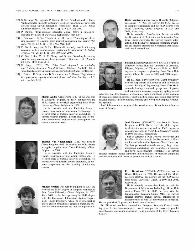
Martin Andre Agnes Fiers (S’10–M’12) was bornin Zottegem, Belgium, in 1985. He received theM.Sc. degree in electrical engineering from GhentUniversity, Ghent, Belgium, in 2008.
He is currently with the Photonics ResearchGroup, Department of Information Technology. Hisresearch topic is photonic reservoir computing. Hiscurrent research interests include modeling of pho-tonic components and software development forcircuit simulation tools.
Thomas Van Vaerenbergh (S’11) was born inGhent, Belgium, 1987. He received the M.Sc. degreein applied physics from Ghent University, Ghent,Belgium, in 2008.
He is currently with the Photonics ResearchGroup, Department of Information Technology. Hisresearch topic is photonic reservoir computing. Hiscurrent research interests include excitability in pho-tonic components and the modeling of microringcircuits.
Francis Wyffels was born in Belgium in 1983. Hereceived the M.Sc. degree in computer engineeringfrom Ghent University, Ghent, Belgium, in 2007.Since 2007, he has been pursuing the Ph.D. degreewith the Electronics Information System Depart-ment, Ghent University, where he is investigatinghow to exploit properties of reservoir computing sys-tems for robot locomotion and time series prediction.
David Verstraeten was born in Brussels, Belgium,on January 17, 1979. He received the M.Sc. degreein computer engineering and the Ph.D. degree fromGhent University, Ghent, Belgium, in 2004 and2009, respectively.
He is currently a Post-Doctoral Researcher withthe Department of Electronics and Information Sys-tems, Ghent University. His current research inter-ests include the study of reservoir computing dynam-ics and machine learning for biomedical applicationsand speech recognition.
Benjamin Schrauwen received the M.Sc. degree incomputer science from the University of Antwerp,Edegem, Belgium, in 2000, and the M.Sc. and Ph.D.degrees in computer engineering from Ghent Uni-versity, Ghent, Belgium, in 2002 and 2008, respec-tively.
He has been a Professor with Ghent Universitywith the Department of Electronics and InformationSystems, Faculty of Engineering, since 2010. He iscurrently leading a research group over 15 peoplewith interests in reservoir computing, spiking neural
networks, and deep learning architectures, with applications in the domainsof speech recognition, robotics, and biomedical signal processing. His currentresearch interests include machine learning and biologically inspired comput-ing systems.
Prof. Schrauwen is a member of the American Association for the Advance-ment of Science.
Joni Dambre (S’99–M’03) was born in Ghent,Belgium, in 1973. She received the M.Sc. degreein electronics engineering and the Ph.D. degree incomputer engineering from Ghent University, Ghent,in 1996 and 2003, respectively.
She is currently a Post-Doctoral Researcher andPart-Time Professor with the Department of Elec-tronics and Information Systems, Ghent University.She has performed research on very large scaleintegration architecture and technology evaluationand novel interconnection techniques. Her current
research interests include hardware implementations of reservoir computingand the computational power of general dynamical systems.
Peter Bienstman (S’97–A’01–M’03) was born inGhent, Belgium, in 1974. He received the M.Sc.degree in electrical engineering and the Ph.D. degreefrom Ghent University, Ghent, in 1997 and 2001,respectively.
He is currently an Associate Professor with theDepartment of Information Technology, Ghent Uni-versity. From 2001 to 2002, he was with theJoannopoulos Research Group, MIT. His currentresearch interests include several applications ofnanophotonics as well as nanophotonics modeling.
He has published 50 papers and holds several patents.Dr. Bienstman has been awarded the European Research Council start-
ing grant for the Naresco-project: Novel paradigms for massively parallelnanophotonic information processing. He is a member of the IEEE PhotonicsSociety.


![IEEE TRANSACTIONS ON NEURAL NETWORKS AND LEARNING …xiaopingwu.cn/assets/paper/tnnls2019_spbl.pdf · 2020-04-20 · 2 IEEE TRANSACTIONS ON NEURAL NETWORKS AND LEARNING SYSTEMS [19],](https://img.pdfslide.us/doc/110x75/5f0ffba07e708231d446db9c/ieee-transactions-on-neural-networks-and-learning-2020-04-20-2-ieee-transactions.jpg)