Embed Size (px)
Citation preview
Coastal Protection and Restoration Authority 450 Laurel Street, Baton Rouge, LA 70804 | [email protected] | www.coastal.la.gov
2017 Coastal Master Plan
Appendix C – Modeling
Attachment C3-4 Barrier Island Model Development (BIMODE)
Report: Version 1
Date: July 2015
Prepared By: Michael Poff (Coastal Engineering Consultants, Inc.), Ioannis Georgiou (University of
New Orleans), Mark Kulp University of New Orleans), Mark Leadon (Coastal Protection and
Restoration Authority), Gordon Thomson (Chicago Bridge & Iron Company), and Dirk Jan Walstra
(Deltares)
2017 Coastal Master Plan: Model Improvement Plan
J u l y 2 0 1 5
P a g e | 2
Coastal Protection and Restoration Authority
This document was prepared in support of the 2017 Coastal Master Plan being prepared by the
Coastal Protection and Restoration Authority of Louisiana (CPRA). CPRA was established by the
Louisiana Legislature in response to Hurricanes Katrina and Rita through Act 8 of the First
Extraordinary Session of 2005. Act 8 of the First Extraordinary Session of 2005 expanded the
membership, duties and responsibilities of CPRA and charged the new Authority to develop and
implement a comprehensive coastal protection plan, consisting of a Master Plan (revised every
5 years) and annual plans. CPRA’s mandate is to develop, implement and enforce a
comprehensive coastal protection and restoration Master Plan.
Suggested Citation:
Poff, M., Georgiou, I., Kulp, M., Leadon, M., Thomson, G., and Walstra, D.J.R., (2015). 2017 Coastal
Master Plan Modeling: Attachment C3-4 – Barrier Island Model Development (BIMODE). Version I.
Baton Rouge, Louisiana: Coastal Protection and Restoration Authority.
2017 Coastal Master Plan: Model Improvement Plan
J u l y 2 0 1 5
P a g e | 3
Acknowledgements
This document was developed as part of a broader Model Improvement Plan in support of the
2017 Coastal Master Plan under the guidance of the Modeling Decision Team:
The Water Institute of the Gulf - Ehab Meselhe, Alaina O. Grace, and Denise Reed
Coastal Protection and Restoration Authority (CPRA) of Louisiana – Angelina Freeman,
David Lindquist, and Mandy Green
A special acknowledgement is offered to Mark Gravens, U.S. Army Corps of Engineers Coastal
Hydraulics Laboratory, for his contribution to the Barrier Island Model Development, especially for
his technical support and guidance on wave transformation processes.
This effort was funded by CPRA of Louisiana under Cooperative Endeavor Agreement Number
2503-12-58, Task Order No. 03.
2017 Coastal Master Plan: Model Improvement Plan
J u l y 2 0 1 5
P a g e | 4
Executive Summary
Predicting the evolution of Louisiana’s barrier islands is a critical component of the Coastal
Protection and Restoration Authority of Louisiana (CPRA) 2017 Coastal Master Plan. The
Integrated Compartment Model (ICM) to be utilized for the 2017 Coastal Master Plan is capable
of efficiently simulating 50-year time periods and predicting project effects at the basin-scale.
The Barrier Island Model Development (BIMODE) component was developed for integration with
the ICM and improves upon the 2012 Coastal Master Plan (CPRA, 2012) barrier shoreline model
by including additional physical processes (e.g., overwash), improving the capabilities of
predicting change in island morphology, and incorporating realistic event-driven
morphodynamic responses.
The scope of work included a literature review, model approach development, and model
formulation, coding, and testing, along with working meetings, routine teleconferences, and
reporting. The focus area includes the Chandeleur Islands on the eastern side of the Mississippi
River active Balize Delta and from Scofield Island to Raccoon Island on the western side of the
Mississippi River active Balize Delta.
Based upon the detailed literature review, knowledge and experience from restoration project
design and field data collection, and professional judgment, the BIMODE Team selected the
following key physical processes, forcing functions, and geomorphic forms for inclusion in the
model: longshore sediment transport, cross-shore sediment transport, breaching, inlets and bays,
post-storm recovery, subsidence, and eustatic sea level rise (ESLR). Descriptions of the processes,
functions, and forms along with their respective analytical and / or empirical formulations are
provided.
Due to the spatial scale of the focus area and the temporal scale of the ICM, complex island
models that predict both longshore and cross-shore sediment transport are not viable. Therefore,
a hybrid modeling approach was developed to account for the key physical processes of
longshore and cross-shore sediment transport. The longshore transport model formulation
includes a three-step wave transformation process using available hindcast data to yield
representative breaking wave conditions. These wave data are used to estimate sediment
transport rates employing the Coastal Engineering Research Center (CERC) transport
formulation.
Sediment sinks are included by not allowing bypassing across specific inlets, that is, assuming
zero transport onto the adjacent downdrift island. Shoreline retreat due to silt loss is computed
based on the percent silt and clay in the erodible face. Varying sand / silt percentages are
allowed on a profile-by-profile basis though uniform percentages were utilized for each island.
The cross-shore sediment transport formulation includes application of the one-dimensional
Storm-induced BEAch CHange (SBEACH) model that simulates cross-shore morphologic response
in response to tropical cyclone events (referred to herein as storms) based on measurement
derived, empirical equations. While the code is not directly incorporated into the BIMODE
model, the SBEACH model runs are recalled through look-up tables to determine the likely
output profile given the starting input profile and storm characteristics. Input profiles are based
on representative static submerged profiles from each of the regions along with combination of
varying dune heights, dune widths and berm widths, some of which represent pre-restoration
barrier island profiles. Barrier island breaching is incorporated into the BIMODE model by
determining critical thresholds of minimum barrier island widths and minimum width to island
length ratios through comparisons to historical data on barrier island breaching.
2017 Coastal Master Plan: Model Improvement Plan
J u l y 2 0 1 5
P a g e | 5
Inlet and bay processes, specifically inlet expansion/enlargement, using equilibrium theory for
inlet cross-sectional area as a function of tidal prism, are incorporated into BIMODE using the
same formulation employed in the 2012 Coastal Master Plan barrier shoreline model (Hughes, et
al., 2012).
Based upon experience in restoration project design, SBEACH tends to under predict storm
erosion, which in some sense accounts for post-storm recovery processes. Accordingly, the
BIMODE Team recommends the post-storm recovery processes are captured sufficiently through
application of SBEACH.
Subsidence and ESLR are incorporated into the BIMODE model through manual adjustments
following guidance documents prepared by CPRA.
The schematization of the BIMODE model outlines the procedure for how the selected physical
processes are incorporated to develop the final output. The procedure includes reading in the
profile and wave data inputs, determining longshore sediment transport, locating nodal points
where sediment transport diverges, determining net erosion or accretion along each profile, and
computing change in beach face profile specific to longshore transport; adjusting beach
profiles to account for relative sea level rise, beach face profile retreat due to silt loss, and
consolidation; accounting for cross-shore sediment transport for the given storm suite; eroding
the bayward side of each profile; checking for and implementing breaching if the thresholds are
met; and incorporating the inlet and bay model; and repeating these steps for the 50-year
simulation period. The output is cross-sections at each emergent profile in the format of a Digital
Elevation Model (DEM).
The BIMODE.f90 program, written in Fortran 90, simulates the physical processes described in the
model schematization. The file structure consists of a main program file, which calls on several
subroutines to run. Each subroutine was tested for functionality. The program in its entirety was
also tested by running 50-year simulations including return interval storms and periods of average
wave conditions. Test runs of the code were successful. Refinements of the code may be
necessary based on the results of the calibration analysis. Calibration outcomes will be reported
in Attachment C3-23 (ICM Calibration and Validation).
2017 Coastal Master Plan: Model Improvement Plan
J u l y 2 0 1 5
P a g e | 6
Table of Contents
Illustrations ........................................................................................................................................................... 9
List of Tables ........................................................................................................................................................ 9
List of Abbreviations ........................................................................................................................................ 11
1.0 Introduction ............................................................................................................................................... 13
1.1 Model Improvement Plan ................................................................................................................ 13
1.2 Scope of Work .................................................................................................................................... 13
1.3 Focus Area .......................................................................................................................................... 14
2.0 Barrier Island Evolution ............................................................................................................................. 16
3.0 Modeling Options for Barrier Island Evolution ..................................................................................... 18
3.1 Summary of 2012 Barrier Shoreline Model .................................................................................... 18
3.2 Review of Model Options ................................................................................................................. 18
3.3 Physical Processes, Forcing Functions, and Geomorphic Forms .............................................. 19
4.0 Wave Transformation ............................................................................................................................... 20
4.1 Input Data ........................................................................................................................................... 20
4.1.1 Wave Climate .......................................................................................................................... 20
4.1.2 Water Level, Tide, and Storm Surge ..................................................................................... 20
4.2 Model Options .................................................................................................................................... 21
4.3 Summary and Recommendations ................................................................................................. 21
4.3.1 General ..................................................................................................................................... 21
4.3.2 Wave Data ............................................................................................................................... 21
4.3.3 WIS Phase III Transformation and Statistical Analysis ........................................................ 23
4.3.4 SWAN Nearshore Wave Transformation .............................................................................. 24
4.3.5 Estimation of Breaking Wave Conditions ............................................................................ 25
5.0 Longshore Sediment Transport .............................................................................................................. 27
5.1 General ................................................................................................................................................ 27
5.2 Model Options .................................................................................................................................... 27
5.2.1 Single Line Theory Models ...................................................................................................... 27
5.2.2 Process Based Morphological Area Models ...................................................................... 30
5.3 Longshore Transport Formulations .................................................................................................. 30
5.4 Summary .............................................................................................................................................. 30
5.5 Calibration Data ................................................................................................................................ 31
2017 Coastal Master Plan: Model Improvement Plan
J u l y 2 0 1 5
P a g e | 7
5.6 Silt Loss .................................................................................................................................................. 34
6.0 Cross-shore Sediment Transport ............................................................................................................. 35
6.1 General ................................................................................................................................................ 35
6.2 Model Options .................................................................................................................................... 35
6.3 Summary .............................................................................................................................................. 37
6.3.1 Model Selection ....................................................................................................................... 37
6.3.2 Calibration Data ...................................................................................................................... 37
6.3.3 Model Implementation .......................................................................................................... 38
7.0 Breaching ................................................................................................................................................... 39
7.1 General ................................................................................................................................................ 39
7.2 Model Options .................................................................................................................................... 39
7.3 Summary .............................................................................................................................................. 41
8.0 Inlets and Bays .......................................................................................................................................... 42
8.1 General ................................................................................................................................................ 42
8.2 Modeling Options .............................................................................................................................. 42
8.2.1 Inlet hydrodynamics ............................................................................................................... 42
8.2.2 Inlet Morphology ..................................................................................................................... 43
8.2.3 Interaction of Inlets with Nearby Environments ................................................................. 44
8.3 Summary .............................................................................................................................................. 45
9.0 Aeolian Processes ..................................................................................................................................... 46
9.1 General ................................................................................................................................................ 46
9.2 Model Options .................................................................................................................................... 46
9.2.1 Bagnold Method ..................................................................................................................... 46
9.2.2 Hsu Method .............................................................................................................................. 47
9.2.3 CEM Method ............................................................................................................................ 48
9.3 Summary .............................................................................................................................................. 49
10.0 Post-Storm Recovery ............................................................................................................................ 51
10.1 General ............................................................................................................................................ 51
10.2 Model Options ................................................................................................................................ 51
10.3 Summary .......................................................................................................................................... 52
11.0 Subsidence ............................................................................................................................................. 53
11.1 General ............................................................................................................................................ 53
11.2 Application for BIMODE ................................................................................................................ 53
2017 Coastal Master Plan: Model Improvement Plan
J u l y 2 0 1 5
P a g e | 8
12.0 Eustatic Sea Level Rise ......................................................................................................................... 56
13.0 Model Schematization ......................................................................................................................... 57
14.0 BIMODE Code Development & Testing ............................................................................................ 60
14.1 Overview .......................................................................................................................................... 60
14.2 BIMODE Code ................................................................................................................................. 60
14.2.1 File Structure .......................................................................................................................... 60
14.2.2 Main Subroutines .................................................................................................................. 61
14.3 Testing ............................................................................................................................................... 63
14.3.1 Profile Data ............................................................................................................................ 63
14.3.2 Wave Transformation .......................................................................................................... 65
14.3.3 Cross-shore Sediment Transport ........................................................................................ 80
14.3.4 Longshore Sediment Transport .......................................................................................... 84
14.3.5 50-year Test Run Based on Monthly Statistic WIS Wave Data ..................................... 88
14.3.6 Inlet and Bay Model Integration ....................................................................................... 94
14.3.7 Program Messages from BIMODE ..................................................................................... 94
14.3.8 Performance ......................................................................................................................... 97
15.0 Conclusions ............................................................................................................................................ 98
16.0 References ........................................................................................................................................... 100
Appendices .................................................................................................................................................... 109
Appendix 1: Review of Barrier Island Model Options ............................................................................. 109
2017 Coastal Master Plan: Model Improvement Plan
J u l y 2 0 1 5
P a g e | 9
Illustrations
List of Tables
Table 1: Proposed Sediment Budget Cells for BIMODE. ........................................................................... 32
Table 2. Barrier Island Breach Data and Breaching Criteria ................................................................... 40
Table 3: Subsidence Values used in 2012 Barrier Shoreline Morphology Model. ................................ 54
Table 4: Bands of Wave Parameters ........................................................................................................... 72
List of Figures
Figure 1: BIMODE Region Map ...................................................................................................................... 14
Figure 2: Study Area Map with Barrier Islands Listed ................................................................................. 15
Figure 3: Three-Stage Geomorphic Model................................................................................................. 16
Figure 4: WIS station locations.. ..................................................................................................................... 22
Figure 5: Single Line Theory According to Pelnard-Considère (1956). .................................................. 28
Figure 6: Reservoir Model for Ebb-Delta Growth and Sand Bypassing Volume Calculation. .......... 45
Figure 7: Map of Projected Subsidence Ranges. ...................................................................................... 54
Figure 8: Model Schematic of Plan Form Processes, Mass Balance of Sediment Transport, and
Corresponding Shoreline Response ............................................................................................................. 55
Figure 9: Plan View of Initial Profile Data Used in Testing.. ....................................................................... 64
Figure 10: ST73124 Hourly Directional Wave Statistics from Jan. 1, 1980 to Dec. 31, 2012. ............... 66
Figure 11: ST73126 Hourly Directional Wave Statistics from Jan. 1, 1980 to Dec. 31, 2012. ............... 67
Figure 12: ST73129 Hourly Directional Wave Statistics from Jan. 1, 1980 to Dec. 31, 2012 ................ 68
Figure 13: ST73131 Hourly Directional Wave Statistics from Jan. 1, 1980 to Dec. 31, 2012 ................ 69
Figure 14: ST73139 Hourly Directional Wave Statistics from Jan. 1, 1980 to Dec. 31, 2012 ................ 70
Figure 15: ST73141 Hourly Directional Wave Statistics from Jan. 1, 1980 to Dec. 31, 2012 ................ 71
Figure 16: SWAN Grid Bathymetry for Isles Dernieres and Timbalier Test .............................................. 72
Figure 17: SWAN Grid Bathymetry for Caminada Headland and Grand Isle Test.............................. 73
Figure 18: SWAN Grid Bathymetry for Barataria Bay Test......................................................................... 73
Figure 19: SWAN Grid Bathymetry for Chandeleur Island and Breton Island Test .............................. 74
Figure 20: SWAN Results of Isles Dernieres and Timbalier for A Single Wave Case ............................. 75
Figure 21: SWAN Results of Caminada Headland and Grand Isle for A Single Wave Case ............ 75
Figure 22: SWAN Results of Barataria Bay for A Single Wave Case ....................................................... 76
2017 Coastal Master Plan: Model Improvement Plan
J u l y 2 0 1 5
P a g e | 10
Figure 23: SWAN Results of Chandeleur Island and Breton Island for A Single Wave Case ............. 76
Figure 24: ST71341 Monthly Offshore Wave Distribution for the Year 1980. .......................................... 77
Figure 25: ST73141 Frequency Distribution of Offshore Wave Statistics for the Year 1980. ................ 78
Figure 26: Monthly Breaking Wave Distribution for Year 1980 at Profile 135 in the Chandeleur
Islands. ............................................................................................................................................................... 79
Figure 27: Frequency Distribution of Breaking Wave Statistics for Year 1980 at Profile 135 in the
Chandeleur Islands. ........................................................................................................................................ 80
Figure 28: SBEACH Results & Transformation Applied in BIMODE. .......................................................... 81
Figure 29: Test Output: Profile Matching in BIMODE ................................................................................. 82
Figure 30: Test Output: Application of Transformation in BIMODE ......................................................... 83
Figure 31: Test Output: Plan View of Shoreline After a 5-Year Storm Event and 20-Year Storm Event84
Figure 32: Test Output: Shoreline Retreat Resulting from Longshore Transport Losses ....................... 85
Figure 33: Test Output: Shoreline Advancement from Longshore Transport Gains ............................ 86
Figure 34: Test Output: Time Series of Shoreline Retreat/Advance ....................................................... 87
Figure 35: Shoreline change after a year of simulation along a section of shoreline on
Chandeleur Island without storm events (left) and the corresponding longshore transport rate
(right). ................................................................................................................................................................ 88
Figure 36: Shoreline and Cumulative Longshore Transport West of Mississippi River (Year 1) .......... 89
Figure 37: Shoreline and Cumulative Longshore Transport West of Mississippi River (Year 20) ........ 89
Figure 38: Shoreline and Cumulative Longshore Transport West of Mississippi River (Year 30) ........ 90
Figure 39: Shoreline and Cumulative Longshore Transport West of Mississippi River (Year 40) ........ 90
Figure 40: Shoreline and Cumulative Longshore Transport West of Mississippi River (Year 50) ........ 91
Figure 41: Shoreline and Cumulative Longshore Transport at Chandeleur Island (Year 1) .............. 91
Figure 42: Shoreline and Cumulative Longshore Transport at Chandeleur Island (Year 10) ............ 92
Figure 43: Shoreline and Cumulative Longshore Transport at Chandeleur Island (Year 20) ............ 92
Figure 44: Shoreline and Cumulative Longshore Transport at Chandeleur Island (Year 30) ............ 93
Figure 45: Shoreline and Cumulative Longshore Transport at Chandeleur Island (Year 40) ............ 93
Figure 46: Shoreline and Cumulative Longshore Transport at Chandeleur Island (Year 50) ............ 94
Figure 47: Successfull Reading of Input File ................................................................................................ 95
Figure 48: Screen View of Program Running .............................................................................................. 96
Figure 49: Normal Termination of Program ................................................................................................. 97
2017 Coastal Master Plan: Model Improvement Plan
J u l y 2 0 1 5
P a g e | 11
List of Abbreviations
ADCIRC
BIMODE
CB&I
CEC
CEM
CERC
CHE
cm
CPE
CPRA
DEM
DHI
ESLR
FEMA
g
hr
IPCC
kg
Lat
Long
m
mm
NAVD
NOAA
NOS
ADvanced CIRCulation Model
Barrier Island Model Development
Chicago Bridge and Iron Company
Coastal Engineering Consultants, Inc.
Coastal Engineering Manual
Coastal Engineering Research Center
Coast & Harbor Engineering, Inc.
Centimeter
Coastal Planning and Engineering, Inc.
Coastal Protection and Restoration Authority
Digital Elevation Model
Danish Hydraulic Institute
Eustatic Sea Level Rise
Federal Emergency Management Agency
Gram
Hour
Intergovernmental Panel on Climate Change
Kilogram
Latitude
Longitude
Meters
Millimeters
North American Vertical Datum of 1988
National Oceanic and Atmospheric Administration
National Ocean Service

2017 Coastal Master Plan: Model Improvement Plan
J u l y 2 0 1 5
P a g e | 12
NRC
RSLR
s
SLR
SBEACH
STWAVE
SWAN
UNO
UnSWAN
USACE
UTM
WIS
yr
National Research Council
Relative Sea Level Rise
Second
Sea Level Rise
Storm-induced BEAch Change Model
Steady-State Spectral Wave Model
Simulating WAves Nearshore Model
University of New Orleans
Unstructured Simulating WAves Nearshore Model
U.S. Army Corps of Engineers
Universal Transverse Mercator
Wave Information Studies
Year
2017 Coastal Master Plan: Model Improvement Plan
J u l y 2 0 1 5
P a g e | 13
1.0 Introduction
1.1 Model Improvement Plan
The Coastal Protection and Restoration Authority of Louisiana (CPRA) embarked on the
development and application of model improvements for the 2017 Coastal Master Plan. This
effort was launched with the 2017 Model Improvement Plan (CPRA, 2013), which builds upon the
modeling developed for the 2012 Coastal Master Plan (CPRA, 2012). The overall vision for the
landscape modeling was to develop an Integrated Compartment Model (ICM) characterized
by development of new process-based algorithms (e.g., marsh edge erosion and sediment
distribution), integration of model code into a single common framework (e.g., all code
integrated into Fortran), and increased resolution of the models (e.g., reducing the size of the
2012 Coastal Master Plan Eco-hydrology compartments). The ICM is designed to simulate 50-
year time periods in an efficient manner and predict project effects at a basin-scale.
Barrier island restoration has been a focus of CPRA’s coastal restoration and protection program
for decades. The ability to predict barrier island morphological dynamics, including long-term
sustainability, is a critical component of this effort. The 2012 barrier shoreline model (Hughes et
al., 2012) was able to predict inlet area change and island movement based on processes such
as wave climate. An external peer review identified that the 2012 barrier shoreline model lacked
dynamic (physical) processes and stochastic events. The improvements identified for the 2017
barrier island model include the addition of physical processes (e.g. overwash), improving the
capabilities of predicting change in island morphology, adding more realistic event-driven
morphodynamic responses, and integration into the ICM.
1.2 Scope of Work
The scope of work for the 2017 Barrier Island Model Development (BIMODE) includes:
Activity 1 – Summarize current literature and available modeling approaches;
Activity 2 – Convene a working meeting to discuss and evaluate modeling approaches;
Activity 3 – Develop the modeling approach and prepare a written summary of the
proposed formulation/approach; and
Activity 4 – Code the model, test the newly developed model, and report results.
This report discusses the physical processes, forcing functions, and geomorphic forms that affect
barrier island evolution in Louisiana; summarizes the current literature specific to the process,
function or form; outlines the analytical and empirical formulations; presents the modeling
approach for the process, function, or form; documents the model schematization for the
BIMODE model; and presents the development of the model coding and testing of the
subroutines to confirm the functionality and accuracy of the program.
2017 Coastal Master Plan: Model Improvement Plan
J u l y 2 0 1 5
P a g e | 14
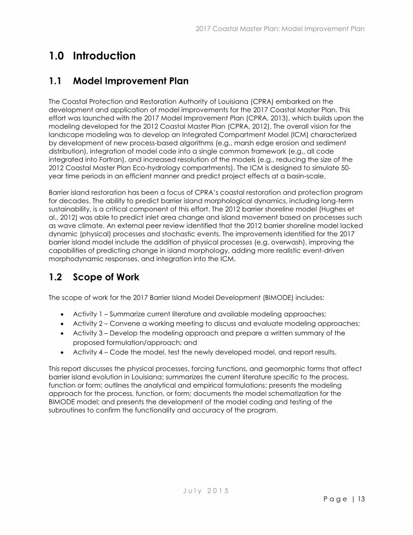
1.3 Focus Area
The focus area (Figure 1) extends from the Chandeleur Islands to the eastern side of the active
Mississippi River Balize Delta and from Scofield Island to Raccoon Island on the western side of
the active Mississippi River Balize Delta. The study area is divided into the following six regions:
Isles Dernieres;
Timbalier;
Caminada Headland and Grand Isle;
Barataria Bay;
Breton Island; and
Chandeleur Island.
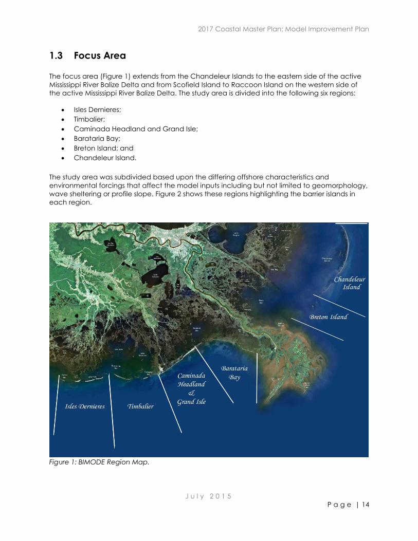
The study area was subdivided based upon the differing offshore characteristics and
environmental forcings that affect the model inputs including but not limited to geomorphology,
wave sheltering or profile slope. Figure 2 shows these regions highlighting the barrier islands in
each region.
Figure 1: BIMODE Region Map.
2017 Coastal Master Plan: Model Improvement Plan
J u l y 2 0 1 5
P a g e | 15
Figure 2: Study Area Map with Barrier Islands Listed.
2017 Coastal Master Plan: Model Improvement Plan
J u l y 2 0 1 5
P a g e | 16
2.0 Barrier Island Evolution
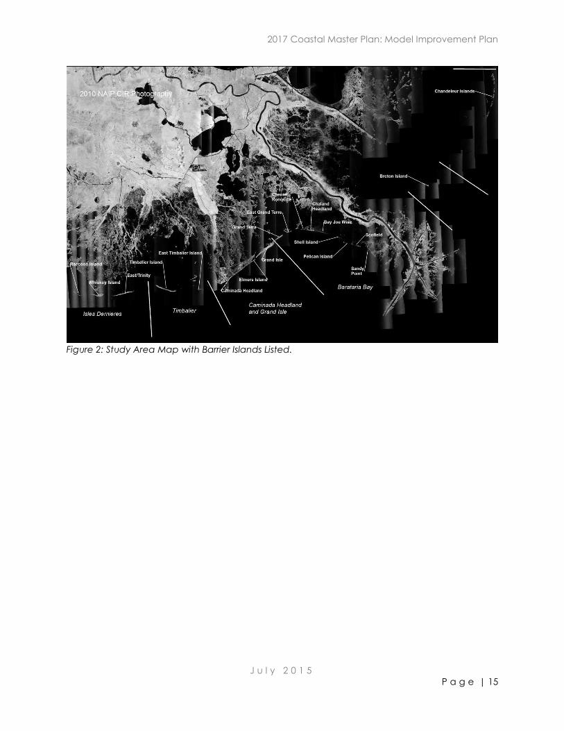
The Louisiana barrier islands are the product of Mississippi River channel switching over the last
5,000 years. It is channel switching and complex interactions between anthropogenic events,
sediment transport, storm impacts, and inlet dynamics that contribute to barrier island formation,
migration, and erosion. Figure 3 presents the three-stage geomorphic model that summarizes
the development and evolution of transgressive depositional systems in the Mississippi River
Deltaic Plain including the formation of the barrier islands (Penland et al., 1988). Due to the lack
of sediment supply, the barrier islands are eroding and degrading. The projected years of
disappearance for the barrier islands are on decadal scales (USACE, 2010 and 2012).
Figure 3: Three-Stage Geomorphic Model.
The evolution of Louisiana’s barrier islands is well described in the literature (e.g., Williams et al.,
1992; Penland et al., 1988; Penland et al., 2005; Georgiou et al., 2005; Kulp et al., 2005; Rosati et
al., 2006 & Rosati and Stone, 2009). Louisiana’s barrier islands are typically low lying and
comprised of three physical features, the beach, dune, and back-barrier marsh. Their
geomorphic form acts as a buffer to reduce the full force and effects of wave action, saltwater
intrusion, storm surge, and tidal currents on associated estuaries and wetlands. Further, the back-
barrier marsh platform captures overwash sediments during episodic events; sediment that
would otherwise be carried into back bay areas to form shoals or be lost into deeper waters. The
marsh also serves as a roll over platform as the islands migrate landward. Their ecologic function
provides wetland habitat for a diverse number of plant and animal species, and to help retain
sediment. The beach and dune are comprised of a thin veneer of sand overlying poorly
consolidated silts and clays. As the elevations of the islands are low, they are frequently
overwashed during storms.
Forcing functions (e.g., winds, waves, tides, currents, subsidence, and eustatic sea level rise
(ESLR)) transport sediment and / or evolve the land forms on a continual basis. Storms impact the
barrier islands as sand is eroded from the Gulf shoreline, the underlying mixed sediments are
exposed to wave attack, and overwash occurs. If a sufficiently wide marsh platform exists, the
2017 Coastal Master Plan: Model Improvement Plan
J u l y 2 0 1 5
P a g e | 17
islands will migrate in an inland direction as washover sediment is captured. As storms pass, the
bayside shoreline or marsh edge may also erode due to waves that are generated on the bay
which transport sediment into the back bay and remove it from the active littoral system. If the
marsh platform is narrow or non-existent, breaches may occur.
In the wake of significant storm events, barrier islands may experience recovery periods, which
are typically years in length and may represent prograding shorelines or may represent periods
where shoreline erosion is less severe than during storm impact periods. While revegetation of
the dune and overwash deposits may occur, the current deteriorated conditions of the majority
of the barrier islands as well as insufficient time between storm events preclude significant
recovery of their geomorphic form and ecologic function.
Louisiana’s barrier islands have a limited sediment supply. In addition, over time the area of the
interior bays has increased as a result of natural and anthropogenic factors (e.g., subsidence, oil
and gas exploration) leading to increases in tidal prism. Increases in the tidal prism jet sediment
further offshore, which increases the ebb shoal capacity and reduces sediment bypassing at
inlets. The ebb shoals are drowned rather than bypassing sand or welding to the adjacent
barriers (Georgiou et al., 2005). New breaches formed during storms typically grow into
permanent inlets, further fragmenting the barrier islands.
For modeling barrier island evolution on decadal scales, Rosati et al. (2006) recommended
accounting for the following: erosion of Gulfside and bayside sand, vegetation, and core
sediments; overwash and washover deposits; breaching; partial recovery of sand along the Gulf
shoreline; vegetation of dunes and wetlands; aeolian transport; longshore sediment transport;
ESLR; subsidence; and consolidation of poorly-consolidated sediment. The approaches to model
these processes are discussed in detail in the following sections of this report.
2017 Coastal Master Plan: Model Improvement Plan
J u l y 2 0 1 5
P a g e | 18
3.0 Modeling Options for Barrier Island Evolution
3.1 Summary of 2012 Barrier Shoreline Model
The 2012 barrier shoreline model (Hughes et al., 2012) simulated coastline and inlet evolution in
response to physical forcings. The model was applied to the sandy shorelines of Louisiana in two
segments. The first segment included the barriers from the western Isle Dernieres (Raccoon
Island) to Scofield Island. The second segment included the barrier islands east of the Mississippi
River delta, including Breton Island and the Chandeleur Islands (Figure 2). The model
encompassed long-term processes, such as response to sea level rise (SLR), subsidence,
landward migration by beach and foreshore erosion and overwash processes, and offshore and
longshore loss of sediment to deepwater sinks below mean annual wave base. The model
operated in a one-dimensional (cross-shore) mode at a selected alongshore interval (~100 m)
and geometrically translated a cross-shore profile based on the calculated processes.
The model used the sediment continuity equation to balance net import or export of sediment,
and then used the deficit or gain to determine the shoreline erosion rate at each location. The
model computed alongshore transport in plan form using an empirical relationship (USACE
2002), driven by offshore wave climate relative to a local shoreline angle. The model used an
annual wave climate derived by analysis of hourly wave information obtained from archived
data from the Wave Information Studies (WIS) project (Hubertz, 1992). The resulting wave climate
was used to drive the longshore transport equation. Resulting net longshore transport was then
balanced by pre-determined cross-shore transport rates, obtained during model calibration. The
resulting mass balance subsequently produced accretion or erosion, depending on excess or a
deficit in the sediment. The result from this procedure was a one-dimensional cross-shore
translation of the shoreline. This process was repeated for each time-step. The model did not
address predictions nearing a century or longer. Further, the model did not account for event
driven (storm induced) change.
The following improvements were recommended for the 2012 barrier shoreline model (Hughes,
2012):
Use of a full local wave model providing more accurate wave heights and directions for
the longshore transport calculations,
In the cross-shore dimension, improve the approach to more accurately account for
overwash processes and removal of sediment offshore,
Account for event driven (storm induced) change, and
Implement more frequent coupling of the eco-hydrology model and the barrier shoreline
model components.
3.2 Review of Model Options
The scope of work for BIMODE began with a review of options for the barrier island model
component of the 2017 Coastal Master Plan ICM, taking into consideration the
recommendations stemming from an external review of the 2012 barrier shoreline model. The
BIMODE Team divided the review of model options into three categories:
Wave Climate and Wave Transformation, Water Level, Tide, and Storm Surge;
2017 Coastal Master Plan: Model Improvement Plan
J u l y 2 0 1 5
P a g e | 19
Sediment Transport and Morphological Change; and
Tidal Inlets and Estuaries/Bays.
The review included the model name, brief description, methodology, pros and cons, and
general discussion as well as summary and discussion on certain inputs for the BIMODE model.
The review served as the first step in recommending the preferred model option for the key
physical processes, forcing functions, and geomorphic forms of longshore sediment transport,
cross-shore sediment transport, and inlets and bays. The selection of the preferred model option
was formulated by outlining specific modeling steps and integrating them into a model
schematization description. With respect to the longshore and cross-shore sediment transport
processes, the BIMODE Team recommended they be handled through separate evaluations
and combined through a hybrid approach.
The complete review is presented in Appendix 1.
3.3 Physical Processes, Forcing Functions, and Geomorphic Forms
Based upon review of pertinent available literature, knowledge and experience from restoration
project design and field data collection, and professional judgment, the BIMODE Team selected
the following physical processes, forcing functions, and geomorphic forms that affect the
evolution of Louisiana’s barrier islands for consideration in developing the modeling approach:
Wave Transformation;
Longshore Sediment Transport;
Cross-shore Sediment Transport;
Breaching;
Inlets and Bays;
Aeolian Processes;
Subsidence;
ESLR; and
Post-Storm Recovery.
These physical processes, forcing functions, consideration of variation in sediment properties,
and geomorphic forms are described in the following sections. The descriptions include pertinent
references describing each process along with relevant literature on recent advances in
modeling specific to BIMODE. The equations and formulations for each process, function or form
incorporated in the BIMODE model are provided. The rationale for not incorporating certain
processes, functions or forms in the BIMODE model is also provided.
2017 Coastal Master Plan: Model Improvement Plan
J u l y 2 0 1 5
P a g e | 20
4.0 Wave Transformation
4.1 Input Data
4.1.1 Wave Climate
Wave data vary in time period and duration and generally include wave height, period, and
direction. Hindcast data are generally longer term time series, e.g. 20-year record, that include
deep water wave data that are generated from wind data. Wave gauge data available for the
Louisiana coast include both deep water and intermediate water locations. Project-specific
gauge data are typically short duration (e.g., monthly) and located in the nearshore. Deep
water is defined where the water depth to wave length ratio is 0.5 or greater. Intermediate
(transitional) water is defined where the water depth to wave length ratio is less than 0.5 and
greater than 0.05. Shallow water is defined where the water depth to wave length ratio is less
than 0.05 (USACE, 2002).
The primary sources of wave input data used in modeling for barrier island studies and project
designs include WIS hindcast time series, Wavewatch III hindcast time series (Tolman, 2009),
National Oceanic and Atmospheric Administration (NOAA) National Data Buoy Center (NDBC)
wave buoys, offshore wave gauge data, project-specific wave measurements, and other
model-generated data. These data sources provide the input to the longshore transport
component of the BIMODE model.
Model generated wave data during tropical storm and hurricane events were produced for the
2012 Coastal Master Plan by ARCADIS using the ADvanced CIRCulation (ADCIRC)
hydrodynamic model coupled with the Unstructured Simulating Waves Nearshore (UnSWAN)
model (CPRA, 2012). Model output included time series of storm surge, water currents, wave
height, wave period, and wave direction at every node in the computational mesh, as well as
the maximum value at any given time step during the simulation. Available storm wave and
storm surge output data was acquired and compiled by CPRA and The Water Institute of the
Gulf for use in the 2017 Coastal Master Plan modeling. These data provide the input to the cross-
shore transport component of the BIMODE model.
4.1.2 Water Level, Tide, and Storm Surge
The primary sources of water level and tide input data used in modeling for barrier island studies
and project designs include NOAA National Ocean Service (NOS) tide gauge data, project-
specific measurements, and other model-generated data. The NOS data generally provide
continuous (6 minute or hourly) time series records over multi-year time intervals. Project specific
measurements also provide continuous time series recordings, but are typically of shorter
duration (e.g., days to months). In addition to daily observed astronomical tide elevation
measurements, storm surge estimates for specific storm events may be generated from the NOS
gauges by subtracting predicted astronomical tide elevations from the observed values.
Storm surge modeling performed for the State of Louisiana and for the Federal Emergency
Management Agency (FEMA) was summarized in the Literature Review (Appendix 1). For
Louisiana barrier island restoration project studies and design, water elevation and storm surge in
cross-shore response modeling have primarily utilized computations and algorithms within the
2017 Coastal Master Plan: Model Improvement Plan
J u l y 2 0 1 5
P a g e | 21
cross-shore models. Storm-specific offshore wave data (from buoys, gauges, and hindcasts) and
nearshore tide gauge data are used as model input.
As with the wave data, the availability of the 2012 Coastal Master Plan output data from the
ADCIRC hydrodynamic model coupled with the UnSWAN wave transformation model was
compiled by CPRA for use in the 2017 Coastal Master Plan modeling. The ADCIRC/UnSWAN
output is used in the cross-shore model simulations for storm events. Non-storm event tidal
fluctuations are incorporated within long-term (decadal) shoreline change simulations based on
longshore sediment transport computations.
4.2 Model Options
Models that transform waves from deep to intermediate water and from intermediate to shallow
water were reviewed and summarized in the initial review of model options (Appendix 1). The
simplified WIS Phase III spectral wave transformation procedure (Jensen, 1983) can be used for
wave transformation from deep water to intermediate water depths. Extensive wave
transformation modeling has been performed as a part of Louisiana’s barrier island restoration
project studies and design (e.g., CPE, 2003; CPE, 2005; CHE, 2007; CEC and SJB, 2008; Thompson,
2008; USACE, 2010; CEC, 2011; and USACE, 2012). The two-dimensional spectral wave models
STWAVE (Smith et al., 2001) and SWAN (Booij et al., 1996) have been primarily used for
intermediate and shallow water wave transformations. Other models including MIKE21 (SW and
NSW) (DHI, 2009) and Delft3D-Wave (Deltares, 2011) have been applied along the Louisiana
coast for specific shallow water wave transformation modeling.
4.3 Summary and Recommendations
4.3.1 General
This section describes the recommended procedure for the wave transformation to be applied
for the estimate of longshore sand transport rates. This procedure including the steps,
techniques, and statistical analyses is based upon review of pertinent available literature,
knowledge and experience from restoration project design, and professional judgment of the
BIMODE Team. The procedure involves the following major steps, which are described in the
following sections:
Selection of Wave Data;
WIS Phase III transformation and statistical analysis;
Detail nearshore wave transformation; and
Estimation of breaking wave conditions.
4.3.2 Wave Data
The BIMODE model requires long-term statistical wave information as input for the estimation of
longshore sand transport rates. The WIS recently completed a comprehensive hindcast for the
Gulf of Mexico for the interval 1980 through 2012. This 33-year wave hindcast is used as the
primary source of wave information for the calculation of longshore sand transport rates in the
BIMODE model. The WIS wave hindcast may be accessed and downloaded from the WIS
website at http://wis.usace.army.mil/.
2017 Coastal Master Plan: Model Improvement Plan
J u l y 2 0 1 5
P a g e | 22
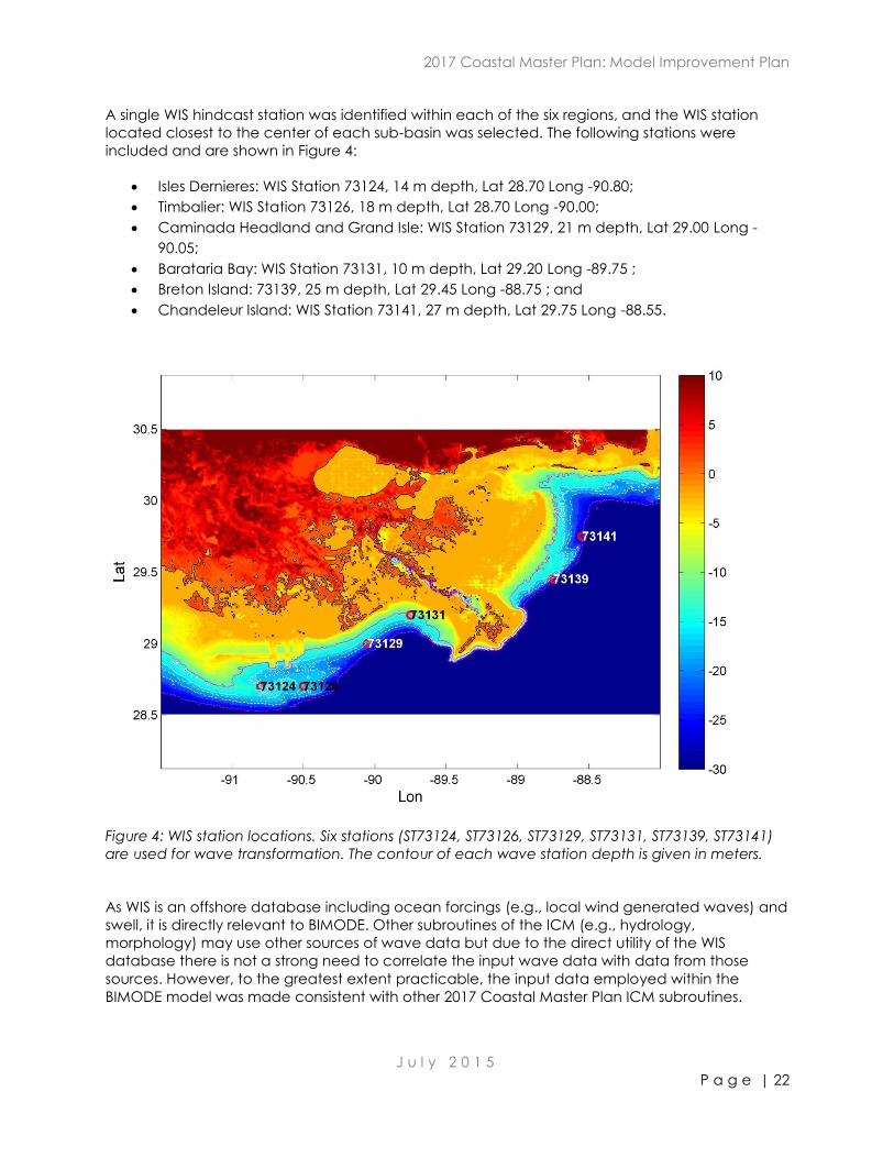
A single WIS hindcast station was identified within each of the six regions, and the WIS station
located closest to the center of each sub-basin was selected. The following stations were
included and are shown in Figure 4:
Isles Dernieres: WIS Station 73124, 14 m depth, Lat 28.70 Long -90.80;
Timbalier: WIS Station 73126, 18 m depth, Lat 28.70 Long -90.00;
Caminada Headland and Grand Isle: WIS Station 73129, 21 m depth, Lat 29.00 Long -
90.05;
Barataria Bay: WIS Station 73131, 10 m depth, Lat 29.20 Long -89.75 ;
Breton Island: 73139, 25 m depth, Lat 29.45 Long -88.75 ; and
Chandeleur Island: WIS Station 73141, 27 m depth, Lat 29.75 Long -88.55.
Figure 4: WIS station locations. Six stations (ST73124, ST73126, ST73129, ST73131, ST73139, ST73141)
are used for wave transformation. The contour of each wave station depth is given in meters.
As WIS is an offshore database including ocean forcings (e.g., local wind generated waves) and
swell, it is directly relevant to BIMODE. Other subroutines of the ICM (e.g., hydrology,
morphology) may use other sources of wave data but due to the direct utility of the WIS
database there is not a strong need to correlate the input wave data with data from those
sources. However, to the greatest extent practicable, the input data employed within the
BIMODE model was made consistent with other 2017 Coastal Master Plan ICM subroutines.
2017 Coastal Master Plan: Model Improvement Plan
J u l y 2 0 1 5
P a g e | 23
4.3.3 WIS Phase III Transformation and Statistical Analysis
The purpose of this step is twofold: first, the deepwater hindcast wave information is processed
to remove offshore traveling wave conditions from the wave time series; and secondly, the
transformed wave data are analyzed to identify statistically representative wave conditions for
each month of the year. Identification and use of statistically representative wave conditions to
characterize the offshore wave climate on a monthly basis is a form of input reduction and is
viewed as imperative to the prediction of barrier island evolution over long time periods (50
years) to avoid excessive computation times.
The WIS Phase III transformation procedure (Jensen, 1983) is a point-to-point spectral wave
transformation procedure that assumes no additional energy input from wind, and straight and
parallel bottom contours. The waves are assumed to have a distribution of energy over a range
of frequencies and directions. The energy spectrum is governed by the Texel, Marsen, and Arsloe
spectral form (Hughes, 1984). The directional spread is given by the cosine function raised to the
4th power. The directional spectrum is discretized into frequency and direction components, and
the components are treated independently. Due to the temporal and spatial scale of the ICM,
the bottom contours between the starting depth and the shallower ending depth are assumed
to be straight and parallel. Application of this assumption is validated through extensive
calibration of the predicted longshore transport rates to measured transport rates. Use of this
transformation procedure is viewed as superior to the alternative of applying a 180 degree cut-
off for offshore traveling waves based on the spectral mean wave direction. In the WIS Phase III
transformation procedure, only the energy in offshore traveling direction bins is removed from
the highly oblique wave conditions and the onshore traveling wave energy is transformed to the
breaking wave water depth of approximately 6 feet.
Selection of the regional shoreline orientation should be done with care as it directly affects the
transformation process. The WIS Phase III transformation technique also allows for sheltering the
shallow water point from wave energy approaching from specified wave directions. This
capability may be important for some of the regions, in particular the Barataria Bay region
(sheltering of wave energy from the east due to the Mississippi River delta), Breton Island region
(sheltering of wave energy from the south and west due to the Mississippi River delta and
sheltering of wave energy from the Mississippi Sound), and Chandeleur Island region (sheltering
of wave energy from the Mississippi Sound).
The Phase III transformation technique is used to transform the offshore wave climate from the
WIS hindcast station to obtain the onshore-directed wave climate at the offshore boundary of
the nearshore transformation model. The Phase III transformation converts the wave angle
convention from meteorological to a shoreline reference angle convention in which wave
angles range between 0 and 180 degrees. In this direction convention, a wave angle of 0
degrees corresponds to a wave traveling parallel to the shoreline from right to left, a wave angle
of 90 degrees corresponds to a wave moving directly on shore (perpendicular to the shoreline),
and a wave angle of 180 degrees corresponds to a wave parallel to shoreline shoreline from left
to right. To convert the wave direction convention to the typical shoreline referenced wave
direction convention, wave angles ranging between +90 and -90 degrees, subtract 90 from the
WIS Phase III wave angle.
After performing the Phase III transformation, the 1980 to 2012 WIS offshore wave time series is
parsed on a monthly basis to obtain 33 data sets for each individual month (January, February,
March, etc.). Each month is analyzed to determine statistically defensible wave conditions for
that month. These conditions essentially represent weighted averages for a 33-year wave
sequence noting the offshore waves are removed as described above. The end goal of the
2017 Coastal Master Plan: Model Improvement Plan
J u l y 2 0 1 5
P a g e | 24
statistical analysis is the identification of different representative wave conditions (based on
bands of wave height, wave period, and incident wave direction) for each month of the year.
Then the wave conditions of the 33 year wave time series are placed in one look-up table.
Repeated wave conditions are neglected. In this way a total of 617 different wave conditions
were defined to characterize the 33 year wave climate within each of the six regions.
Statistical analysis includes:
Use of wave period bands: minimum period to 4 seconds, 4-6 seconds, 6-8 seconds, 8-10
seconds, 10-12 second, etc. up to maximum wave period
Use of wave direction bands at 22.5º angles (N, NNE, NE, ENE… NNW)
Wave height bands (for significant wave height) defined in 1m increments: 0-0.5m, 0.5-
1.5m, 1.5-2.5m, 2.5-3.5m, etc., up to the maximum wave height
This is a typical wave breakdown for GENESIS modeling (Hanson and Kraus, 1991) and follows
guidance for the hypercube method (Bonanata et al, 2010).
These divisional bands were selected to provide representative wave conditions in a manner
that would provide computational efficiency given the geographical extent of the BIMODE
model. The wave period division distinctly encompasses both more frequent, lower energy wave
conditions, as well as, less frequent waves during more energetic conditions. Application of
these monthly wave conditions incorporates seasonal and time sequencing influences into the
wave conditions for the BIMODE model.
4.3.4 SWAN Nearshore Wave Transformation
The BIMODE Team considered both the Steady-State Spectral WAVE model (STWAVE) (Smith et
al., 2001) and Simulating WAves Nearshore (SWAN) model (Booij et al., 1996) as candidate
nearshore wave transformation models from the offshore boundary to near breaking conditions.
Both models are robust computationally efficient tools for estimating the transformation of waves
across an irregular nearshore bathymetry. The BIMODE Team decided to use the SWAN
nearshore wave transformation model due to the familiarity with the model and previous use of
SWAN in the design and performance evaluation of barrier island restoration projects in the
focus area. The SWAN model is used to transform the representative wave conditions across the
irregular nearshore bathymetry from the WIS Stations to near breaking conditions. The SWAN
model includes wave damping, shoaling, refraction, and breaking. Further, storm surge is
included in the SWAN model.
For these simulations, a unit input wave height is specified together with the mean wave period
and mean wave direction computed from the statistical analysis. Pre-breaking wave conditions
in the nearshore are saved corresponding to the specific profiles (shoreline segments) that
evolve using the BIMODE model. By transforming a unit wave height, the resulting wave height in
the nearshore can be viewed as a transformation coefficient (product of the refraction and
shoaling coefficients) and can be multiplied by the mean wave height calculated for each of
the wave height bands to obtain unique nearshore wave heights. The save stations for
nearshore wave conditions should be located in pre-breaking water depths for the majority of
the wave conditions. It is necessary that the save stations be located in pre-breaking water
depths in order for the assumptions associated with the unit wave height transformation
procedure to be valid. It was recommended that the save stations be located in water depths
generally greater than 3 m and less than 5 m to the extent that this is possible and practical.
2017 Coastal Master Plan: Model Improvement Plan
J u l y 2 0 1 5
P a g e | 25
Output from this step of the wave transformation procedure is a database of nearshore wave
information including wave height, wave period, wave angle, nearshore station depth, and
percent occurrence for each month of the year. The number of required SWAN simulations
depended on the number of statistically represented wave conditions identified in the statistical
analysis of the offshore time series of wave conditions. The maximum was 120 conditions (two
wave period bands by 5 wave direction bands by 12 months) for each of the six regions.
4.3.5 Estimation of Breaking Wave Conditions
Final wave transformation to breaking is performed within the BIMODE model using a breaking
wave criteria, Snell’s Law, and the conservation of wave energy. In this portion of the analysis,
the wave angle with respect to the local shoreline orientation is estimated based on shoreline
positions at adjacent modeled profiles. The nearshore waves are transformed to breaking with
respect to the local shoreline orientation and the resulting breaking wave conditions are used to
estimate longshore sand transport rates for each of the representative monthly wave conditions.
Application of the breaking wave criteria is validated through extensive calibration of the
longshore transport rates. Further, the uncertainties in the wave transformation process are far
less than the overall calibration of longshore transport to obtain realistic transport rates.
The pertinent equations used in this phase of the wave transformation procedure are as follows:
Conservation of Wave Energy
2211 coscos gg CECE (Eqn. 1)
Where: E = wave energy density
gC = wave group velocity
= wave angle relative to shore normal
Subscripts 1 and 2 denote different water depths,
and
2
8
1HgE (Eqn. 2)
where:
= mass density of water
g = gravitational acceleration
H = wave height,
and
nCCg (Eqn. 3)
where: C = wave phase velocity
n = ratio of wave group velocity to wave phase velocity,
and
2017 Coastal Master Plan: Model Improvement Plan
J u l y 2 0 1 5
P a g e | 26
T
LC (Eqn. 4)
where: L = wave length
T = wave period,
and
hk
hkn
2sinh
21
2
1 (Eqn. 5)
where: k = wave number
h = water depth,
and
Lk
2 (Eqn. 6)
Breaking Wave Criterion
bb hH 78.0 (Eqn. 7)
Where: bH = Breaking wave height
bh = water depth at breaking.
Snell’s Law
2
2
1
1 sinsin
LL
(Eqn. 8)
Wave Length
L
hTgL
2tanh
2
2
(Eqn. 9)
While more sophisticated wave breaking criteria are available, Hunt’s equation (approximation)
can be used to provide an explicit solution (Hunt, 1979). Based upon the detailed literature
review, knowledge and experience from field data collection and numerical modeling of wave
transformation and breaking, and professional judgment, the BIMODE Team deemed this
approach sufficient for the temporal and spatial scales of the ICM.
2017 Coastal Master Plan: Model Improvement Plan
J u l y 2 0 1 5
P a g e | 27
5.0 Longshore Sediment Transport
5.1 General
Longshore sediment transport is defined as the movement of sediment parallel to the shoreline
occurring primarily within the surf zone under the forcing functions of breaking waves and surf
combined with nearshore currents. This process is one of the key physical processes that controls
beach morphology and is at the core of the BIMODE model. It interacts with the other key
processes, forcing functions, and geomorphic forms including cross-shore sediment transport
and inlets and bays.
Waves reach the shoreline from different directions and produce daily as well as seasonal
reversals in transport direction. The gross transport rate is defined as the summation of sediment
transport in both the left and right directions (along the shoreline) and may be used in estimating
shoaling rates in inlets and channels. The net transport rate is defined as the difference between
left and right directed sediment transport, the higher value indicating the net direction of
transport. It is the gradient of the net sediment transport rate that is used to estimate the retreat
or advance of the shoreline.
While the full longshore transport potential may not be realized on Louisiana’s sediment starved
coast, application of a longshore transport formulation with calibration to measured transport
rates accounts for sediment deprivation. For the purpose of the model, it was assumed that
barrier island recession releases a sufficient supply of sand to satisfy the longshore transport
potential provided extensive calibration to published data is performed and the release and loss
of silt is accounted for.
5.2 Model Options
5.2.1 Single Line Theory Models
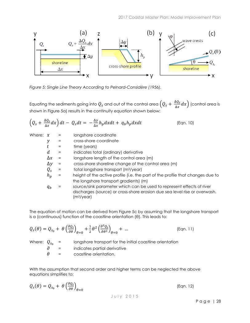
The theory of Pelnard-Considère (1956) gives the basic equations describing the morphological
processes of coastline evolution due to longshore sediment transport gradients (Figure 5a). These
equations lead to the well-known diffusion equation derived below. For the single line theory, the
coastal profile is schematized according to Figure 5.
2017 Coastal Master Plan: Model Improvement Plan
J u l y 2 0 1 5
P a g e | 28
Figure 5: Single Line Theory According to Pelnard-Considère (1956).
Equating the sediments going into 𝑄𝑠 and out of the control area (𝑄𝑠 + Δ𝑄𝑠
Δ𝑥𝑑𝑥) (control area is
shown in Figure 5a) results in the continuity equation shown below:
(𝑄𝑠 + Δ𝑄𝑠
Δ𝑥𝑑𝑥) 𝑑𝑡 − 𝑄𝑠𝑑𝑡 = −
Δ𝑦
Δ𝑥ℎ𝑝𝑑𝑥𝑑𝑡 + 𝑞𝑏ℎ𝑝𝑑𝑥𝑑𝑡 (Eqn. 10)
Where: 𝑥 = longshore coordinate
𝑦 = cross-shore coordinate
𝑡 = time (years)
𝑑 = indicates total (ordinary) derivative
Δ𝑥 = longshore length of the control area (m)
Δ𝑦 = cross-shore shoreline change of the control area (m)
𝑄𝑠 = total longshore transport (m3/year)
ℎ𝑝 = height of the active profile (i.e. the part of the profile that changes due to
the longshore transport gradients) (m)
𝑞𝑏 = source/sink parameter which can be used to represent effects of river
discharges (source) or cross-shore erosion due sea level rise or overwash.
(m3/year)
The equation of motion can be derived from Figure 5c by assuming that the longshore transport
is a (continuous) function of the coastline orientation (θ). This leads to:
𝑄𝑠(𝜃) = 𝑄𝑠0+ 𝜃 (
𝜕𝑄𝑠
𝜕𝜃)
𝜃=0+
1
2𝜃2 (
𝜕2𝑄𝑠
𝜕𝜃2 )𝜃=0
+ … (Eqn. 11)
Where: 𝑄𝑠0 = longshore transport for the initial coastline orientation
𝜕 = indicates partial derivative
𝜃
= coastline orientation.
With the assumption that second order and higher terms can be neglected the above
equations simplifies to:
𝑄𝑠(𝜃) = 𝑄𝑠0+ 𝜃 (
𝜕𝑄𝑠
𝜕𝜃)
𝜃=0 (Eqn. 12)
2017 Coastal Master Plan: Model Improvement Plan
J u l y 2 0 1 5
P a g e | 29
Assuming small angles:
𝜃 = tan 𝜃 = 𝜕𝑥
𝜕𝑦 (Eqn. 13)
and defining
−𝜕𝑄𝑠
𝜕𝜃= 𝑆1 (Eqn. 14)
the longshore transport can be described as a function of the coastline orientation (equation of
motion):
𝑄𝑠(𝜃) = 𝑄𝑠0− 𝑆1
𝛿𝑦
𝛿𝑥 (Eqn. 15)
Where: 𝑆1 = the variation of the transport as a function of the coastline orientation.
Combining Equations 10 and 15, a simple diffusion equation results (Equation 16) that describes
the coastline behavior in combination with a source/sink term:
−𝛿𝑦
𝛿𝑡=
𝑆1
ℎ𝑝
𝛿2𝑦
𝛿𝑥2 + 𝑞𝑏
(Eqn. 16)
A detailed description of single line theory models including empirical, analytical and numerical
approaches is found in USACE (2002).
Although single line theory models, termed coastline models herein, are a very useful tool for the
prediction of long term coastal behavior on decadal time scales, some of the assumptions may
limit their applicability in certain situations. Of major importance is the assumption that the
shoreline erosion or accretion is derived from the horizontal movement of the cross-shore profile
including the beach, defined as the toe of dune to mean low water, and the shoreface,
defined from mean low water to point where beach sand actively oscillates due to wave
conditions, is assumed to move horizontally over its entire active profile height, ℎ𝑝. Refer also to
Figure 5b. The beach slope, therefore, does not change. Also, beyond the active profile height,
the bottom does not move. The shoreward limit of profile change is located at the top of the
active profile. Important implications of this assumption are that only longshore sediment
transports are accounted for and that the cross-shore profiles are assumed to be in equilibrium.
Additional processes that may influence the coastline development (e.g., interaction with
adjacent inlets or breaching, overwash and post-storm recovery) can be incorporated in the
source and sink term in the above equation (𝑞𝑏). Only the aggregated sediment volume that
affects the coastline response should be incorporated. This implies that the coupling of the
coastline model to inlet models and/or cross-shore profile models requires the
aggregation/transformation of potentially complex model outcomes to a single volume source
or sink rate.
2017 Coastal Master Plan: Model Improvement Plan
J u l y 2 0 1 5
P a g e | 30
5.2.2 Process Based Morphological Area Models
More advanced process based morphological area models are available (e.g., Delft3D, MIKE21,
MIKE3). However, the spatial and temporal time scales of the 2017 modeling effort exceed their
practical application range. Despite the fact that these models include many detailed
hydrodynamic and transport processes, they are often unable to accurately describe the long
term coastline evolution (e.g., Van Duin et al., 2004 and Grunnet et al., 2004). Although progress
has been made to simulate cross-shore profile morphology within these morphological area
models (e.g., Ruessink et al., 2007 and Walstra et al., 2012), such process based models require a
significant calibration effort.
5.3 Longshore Transport Formulations
Many longshore transport formulations have been developed (e.g., see Bodge (1989) for an
overview). All are based on the dual presence of a stirring mechanism (waves) and advective
mechanism (longshore). The first transport formulations were based on the total transport
concept (i.e., no distinction between suspended and bed load transport components) and
usually considered the cross-shore integrated transports (referred to as bulk transports, such as
the Coastal Engineering Research Center (CERC), 1984 and Kamphuis, 2000). More advanced
transport formulations distinguished between bed load and suspended load (Bijker, 1967, 1971;
Van Rijn,1993; and Soulsby, 1997) and even fine material (Van Rijn, 2007a and 2007b). The
advanced transport formulations require estimates of the cross-shore wave height distribution,
(breaking) wave induced longshore current, orbital velocities, etc. Furthermore, some
formulations also include cross-shore transport processes due to wave asymmetry (Van Rijn,
2007a and 2007b).
CERC (1984) bulk equation (only waves);
Kamphuis (2000) bulk equation;
Bijker (1967, 1971) bed and suspended load of sand;
Van Rijn (1993) bed and suspended load of sand;
Soulsby (1997) bed and suspended load of sand; and
Van Rijn (2007a and 2007b) bed and suspended load of sand and fine sediment.
5.4 Summary
Using a single morphological area model application, e.g., MIKE21(DHI, 2009) or Delft3D-Wave
(Deltares, 2011), covering the entire study area to simulate barrier shoreline change on a
decadal scale would constitute an unprecedented (and impracticably large) computational
effort. In contrast, a coastline model application, e.g. longshore transport formulation utilizing
CERC (1984), was considered more suitable for the envisaged large spatial and temporal scale
applications in the BIMODE model. However, care should be taken not to apply the BIMODE
model or use its results beyond its applicability range.
Known limitations of utilizing a coastline model within BIMODE include:
Assuming a similar alongshore grid resolution as the 2012 model of about 100 m, features
or impacts on scales of less than 300 to 500 m cannot accurately be resolved.
If longshore transport calculations are updated every time step to coincide with the
monthly breaking wave output time steps described in Section 4, predicted temporal
changes on similar or smaller time scales may be less accurate.
2017 Coastal Master Plan: Model Improvement Plan
J u l y 2 0 1 5
P a g e | 31
Gradients in longshore transport should be the main driver of coastline change because
coastline models assume a constant cross-shore profile shape. Therefore, breaching,
overwash or adjacent inlets should have a relatively small effect on the longshore
transport.
Successful calibrated shoreline change simulations on complex barrier islands using coastline
models have been performed extensively (e.g., Leadon, 1991, 1995; USACE, 2004; CPE, 2005;
CHE, 2007; and CEC, 2011). It should be noted that successful calibration of coastline models
does require significant effort and care. The application of coastline modeling within the
BIMODE modeling approach improves upon coastline modeling applied for the 2012 barrier
shoreline model by including process-based modeling of wave transformation described in
Section 4 and cross-shore sediment transport described in Section 6.
Despite the advances that have been made in recent years (e.g., Van Rijn et al., 2013),
longshore transport calculations (and as a result the coastline evolution considered here) still
require a substantial calibration effort. Especially in complex coastal settings such as the
Louisiana coast (e.g. multiple sediment types, inlets, extreme forcing conditions), the prediction
uncertainties increase dramatically. This also applies to predictions based on advanced
practical transport formulations, which would therefore still require a significant calibration. In
other words, it is unlikely that advanced transport models would reduce the calibration effort.
Furthermore, simple formulations such as CERC and Kamphuis have a predictable behavior,
which facilitates the calibration effort. Complex formulations have the disadvantage of a
relatively large number of model parameters and the (combined) effects of these on the model
outcomes are not always clear.
Therefore, assuming that a calibration effort with historical shoreline changes is not influenced by
the choice of the longshore transport formulation, the application of a simple transport
formulation is preferred. The CERC equation is straightforward to code; was previously reviewed,
accepted, and applied in the 2012 barrier shoreline model; and was preferred by the BIMODE
Team based on personal experience.
Based on the above considerations, the CERC transport formulation is included in the BIMODE
model with alongshore varying (site specific) calibration factors derived from an extensive
calibration with observed shoreline change and longshore transport rates. Specifically the
empirical coefficient (K value) in the transport formulation is calibrated to yield predicted
transport rates on the same order of magnitude as the published longshore transport rates.
5.5 Calibration Data
A sediment budget is a method to track the location and movement of sediment within a
system. The “system” can be broken into various cells, which along with the entire system, are
defined by the developer of the sediment budget. The sediment budget can include sources
that provide sediment to the system or sinks, which remove sediment from the system.
For the purposes of BIMODE, a sediment budget is applied to define the transport of sediment
along various reaches and determine whether the inlets act as a complete sediment sink or
whether there is sediment transport across the inlet. Rosati (2009) developed a sediment budget
for all of coastal Louisiana, which included sediment within interior bays and sediment located
beyond the depth of closure. Morang et al. (2013) expanded upon this budget and can provide
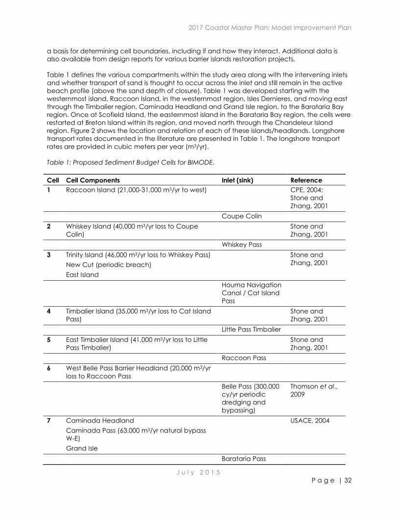
2017 Coastal Master Plan: Model Improvement Plan
J u l y 2 0 1 5
P a g e | 32
a basis for determining cell boundaries, including if and how they interact. Additional data is
also available from design reports for various barrier islands restoration projects.
Table 1 defines the various compartments within the study area along with the intervening inlets
and whether transport of sand is thought to occur across the inlet and still remain in the active
beach profile (above the sand depth of closure). Table 1 was developed starting with the
westernmost island, Raccoon Island, in the westernmost region, Isles Dernieres, and moving east
through the Timbalier region, Caminada Headland and Grand Isle region, to the Barataria Bay
region. Once at Scofield Island, the easternmost island in the Barataria Bay region, the cells were
restarted at Breton Island within its region, and moved north through the Chandeleur Island
region. Figure 2 shows the location and relation of each of these islands/headlands. Longshore
transport rates documented in the literature are presented in Table 1. The longshore transport
rates are provided in cubic meters per year (m3/yr).
Table 1: Proposed Sediment Budget Cells for BIMODE.
Cell Cell Components Inlet (sink) Reference
1 Raccoon Island (21,000-31,000 m3/yr to west) CPE, 2004;
Stone and
Zhang, 2001
Coupe Colin
2 Whiskey Island (40,000 m3/yr loss to Coupe
Colin)
Stone and
Zhang, 2001
Whiskey Pass
3 Trinity Island (46,000 m3/yr loss to Whiskey Pass)
New Cut (periodic breach)
East Island
Stone and
Zhang, 2001
Houma Navigation
Canal / Cat Island
Pass
4 Timbalier Island (35,000 m3/yr loss to Cat Island
Pass)
Stone and
Zhang, 2001
Little Pass Timbalier
5 East Timbalier Island (41,000 m3/yr loss to Little
Pass Timbalier)
Stone and
Zhang, 2001
Raccoon Pass
6 West Belle Pass Barrier Headland (20,000 m3/yr
loss to Raccoon Pass
Belle Pass (300,000
cy/yr periodic
dredging and
bypassing)
Thomson et al.,
2009
7 Caminada Headland
Caminada Pass (63,000 m3/yr natural bypass
W-E)
Grand Isle
USACE, 2004
Barataria Pass
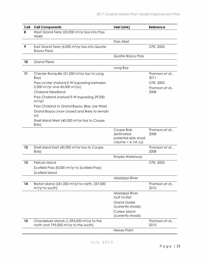
2017 Coastal Master Plan: Model Improvement Plan
J u l y 2 0 1 5
P a g e | 33
Cell Cell Components Inlet (sink) Reference
8 West Grand Terre (23,000 m3/yr loss into Pass
Abel)
Pass Abel
9 East Grand Terre (4,000 m3/yr loss into Qautre
Bayou Pass)
CPE, 2005
Quatre Bayou Pass
10 Grand Pierre
Long Bay
11 Chenier Ronquille (31,000 m3/yr loss to Long
Bay)
Pass La Mer (natural E-W bypassing between
2,500 m3/yr and 45,000 m3/yr)
Chaland Headland
Pass Chaland (natural E-W bypassing 29,000
m3/yr)
Pass Chaland to Grand Bayou (Bay Joe Wise)
Grand Bayou (now closed and likely to remain
so)
Shell Island West (40,000 m3/yr loss to Coupe
Bob)
Thomson et al.,
2011
CPE, 2003
Thomson et al.,
2008
Coupe Bob
(estimated
potential ebb shoal
volume = 4.1M cy)
Thomson et al.,
2008
12 Shell Island East (40,000 m3/yr loss to Coupe
Bob)
Thomson et al.,
2008
Empire Waterway
13 Pelican Island
Scofield Pass (8,000 m3/yr to Scofield Pass)
Scofield Island
CPE, 2003
Mississippi River
14 Breton Island (241,000 m3/yr to north, 237,000
m3/yr to south)
Thomson et al.,
2010
Mississippi River
Gulf Outlet
Grand Gosier
(currently shoals)
Curlew Island
(currently shoals)
15 Chandeluer Islands (1,093,000 m3/yr to the
north and 795,000 m3/yr to the south)
Thomson et al.,
2010
Hewes Point
2017 Coastal Master Plan: Model Improvement Plan
J u l y 2 0 1 5
P a g e | 34
The estimates of sediment transport are used to calibrate longshore sediment transport
developed in the BIMODE model. This calibration is for existing conditions only. The
compartments listed above are used to determine the terminal end of longshore transport and
essentially the terminus of the barrier system. These are applied at the start of the model with
island breaching being applied at a later time step, as discussed in Section 7. The sediment
transport rates are also used to determine growth at non-structured ends of the system. As the
modeling effort proceeds, additional calibration data may be identified to complete blank cells.
It is noted the longshore transport rates for the Breton Island and Chandeleur Island regions are
an order of magnitude greater than the other regions, which is attributed to the acute wave
angle, relatively deep depth of closure on the order of 30 feet, and profile steepness.
5.6 Silt Loss
Louisiana's barrier islands are composed of sand, silt, and clay. The composition of the erodible
face of the island must be considered when predicting future shoreline recession because silt
and clay exposed along the Gulf shoreline face are placed in suspension and transported
offshore, while the sand fraction remains behind. This sand fraction is then subjected to
longshore transport. From a coastal engineering perspective, it is the volume of sand within the
system that is important because the sand provides protection from wave attack. The cohesive
nature of the silt/clay soil is ignored over the longer term. Marsh outcroppings are exposed along
the shoreface following storm conditions suggesting that sand overwashes the island while the
cohesive soils may survive the initial passage of the storm. However, the marsh outcrops are then
eroded rapidly under average wave conditions reforming a sandy gulf shoreline face well
landward of the pre-storm condition The shoreline retreat in the weeks following a storm has
been observed to be as large as the retreat during the passage of the storm (Penland et al.,
2005).
A non-restored island has higher silt content in the erodible beach face than a restored island.
Campbell (2005) suggested that marsh samples should be taken to estimate the silt content in
the erodible face of a non-restored island. A sample from within the marsh is a better
representation of the erodible face as the shoreline may at one point be at this location with the
transient beach face. The silt content in the erodible face of a restored island varies depending
on the silt content of the borrow area and whether the beach was constructed in front of the
original island or on top of the original island.
Therefore, in addition to shoreline retreat that is determined from the longshore sediment
transport rates, shoreline retreat due to silt loss is also computed within the BIMODE model. An
estimate of the shoreline retreat is developed based on the percent silt and clay in the erodible
face. For example, if a non-restored island with 50% silt and clay is expected to retreat 0.3 m due
to longshore transport, the actual shoreline recession is estimated at 0.6 m (1/(1-50%)). However,
a restored island with a silt content of 10% retreats 0.33 m for the same 0.3 m estimate of
shoreline retreat due to longshore transport (1/(1-10%)).
This theory is based on the dynamic morphosedimentary model by Campbell (2005), which
postulated that absent a catastrophic event, the shoreline recession during the storm is
matched or exceeded by the recession in the months following the storm. This is attributed to the
exposed cohesive sediment withstanding the larger waves due to the limited time element but
then eroding under constant but smaller waves and the abrasiveness provided by the sand
fraction remaining on the shoreface.
2017 Coastal Master Plan: Model Improvement Plan
J u l y 2 0 1 5
P a g e | 35
6.0 Cross-shore Sediment Transport
6.1 General
Cross-shore sediment transport typically refers to a barrier island’s profile response to storm
events, though profile shaping and retreat also occur during quiescent periods. Given the low
elevation of Louisiana’s barrier islands, the storm surge and runup can exceed the island crest
elevation during storm events. De Sonneville (2006) showed that once Louisiana’s barrier islands
are overtopped then the sediment transport is predominantly bayward resulting in overwash.
Campbell (2005) suggested that overwash stripped the sand veneer from the face of Louisiana’s
barrier exposing the mixed deltaic sediments, which once exposed experienced high retreat
rates until sufficient sand was released to reform the sand veneer. Campbell’s theory postulated
that the more cohesive sediment withstands the storm event better than the non-cohesive
sediment (sand) but in the months following the passing of the storm, the cohesive sediment is
essentially abraded away by sand being rubbed across the surface by regular waves. This
releases more sand from the mixed deltaic sediment contained within the island core. Once
there is sufficient sand on the shoreface, this loss of cohesive sediment slows as the sand covers
it. Thus rebuilding Louisiana’s barrier islands higher/wider with sand should increase sustainability
and longevity.
Other cross-shore transport processes that can rebuild / add elevations include recovery after
storms and aeolian processes, and are discussed separately in subsequent chapters.
As part of the model development, the BIMODE Team focused the model approach on the
recommendations from the review of barrier island model options (Appendix 1). Specifically, the
longshore and cross-shore sediment transport processes are handled separately through a
hybrid approach. One of the primary recommendations for improving the 2012 barrier shoreline
model was the inclusion of cross-shore processes (e.g., overwash) and thus the BIMODE Team
focused a significant work effort on the addition of cross-shore transport processes.
6.2 Model Options
Overwash is one of the major cross-shore transport processes that drives the morphology of
Louisiana’s barrier islands. Several models are available that can predict the islands’ response to
storms. A discussion of these models follows.
EDUNE: EDUNE was developed by Kriebel (1995) with Robert Dean as an early collaborator. It is a
cross-shore, one-dimensional model that is based on Dean’s equilibrium profile theory and uses a
finite difference solution. It is an open source code. While quick and easy to apply, it does not
include overwash.
Beach-fx: Beach-fx (Gravens et al., 2007) is the USACE’s Monte Carlo simulation model for
estimating the physical performance and economic benefits and costs of shore protection
projects, particularly beach nourishment along sandy shores. It is a cross-shore, one-dimensional
model that simulates cross-shore morphologic response to a storm event based on
measurement derived, empirical equations. It is a widely used model that has been applied
extensively along the Atlantic and Gulf of Mexico developed coastlines to estimate beach
erosion and dune lowering and evaluate beach nourishment project performance. While not an
open source code, it is possible to run hundreds of simulations quickly. Its limitation includes the
2017 Coastal Master Plan: Model Improvement Plan
J u l y 2 0 1 5
P a g e | 36
specified berm elevation is fixed and not allowed to vary throughout the simulated lifecycle.
Further, breaching is not simulated in Beach-fx.
Delft3D: Delft3D (Deltares, 2011) is one of the more advanced two- or three-dimensional models
available for modeling coastal processes. Delft3D incorporates the majority of coastal processes
related to waves, winds, currents, water levels, and sediment transport. While it can incorporate
overtopping and overwash of the islands, it is computationally intensive requiring longer run
times. For example, running a 20-year wave climate for the Chenier Ronquille Barrier Island
Restoration project required approximately one week (Thomson et al., 2011). It is an open source
code.
XBeach: XBeach (Roelvink et al., 2009) is a two-dimensional model for wave propagation, long
waves and mean flow, sediment transport and morphological changes of the nearshore area,
beaches, dunes and back-barrier during storms. It is an open source code model that has been
developed with funding and support by the USACE and a consortium of UNESCO-IHE, Deltares
(Delft Hydraulics), Delft University of Technology, and the University of Miami. The model solves
coupled two-dimensional horizontal equations for wave propagation, flow, sediment transport
and bottom changes, for varying (spectral) wave and flow boundary conditions. Because the
model accounts for the temporal variation in wave height, it resolves the long-wave motions
created by this variation. This so-called ‘surf beat’ is responsible for most of the swash waves that
actually hit the dune front or overtop it. With this innovation, the XBeach model is better able to
model the development of the dune erosion profile, to predict when a dune or barrier island will
start overwashing and breaching, and to model the developments throughout these phases.
However, this model has not been frequently applied to Louisiana’s barrier islands; thus
significant time and expense would be required to calibrate and validate its utilization for
coastal Louisiana.
MIKE21 and MIKE3: MIKE21 and MIKE 3 (DHI, 2009) models are the two-dimensional and three-
dimensional versions of the MIKE suite that use spectral waves and radiation stress to drive
sediment transport. These models incorporate the majority of coastal processes related to
waves, winds, currents, water levels, and sediment transport. While they can incorporate
overtopping and overwash of the islands, the computing time is extensive and the run times are
long. The model code is not open source.
SBEACH: SBEACH was developed by the USACE and is operated within the Coastal Engineering
Design and Analysis System user interface (Larson and Kraus, 1989). It is a cross-shore, one-
dimensional model that simulates cross-shore morphologic response in response to a storm event
based on measurement derived, empirical equations. Within SBEACH, volume is conserved. It is a
widely used model that has been applied extensively in coastal Louisiana to estimate dune
lowering and overwash extents across barrier islands. While not an open source code, which
negates the ability to include the code directly into the model, it is possible to run hundreds of
simulations quickly. These runs can then be recalled through a look-up table to determine the
likely output profile given the starting input profile and storm characteristics. The model has the
ability to predict the cross-shore transport and overwash physical processes, has been used
extensively in the design of Louisiana barrier island restoration projects, and is capable of running
hundreds of simulations cost effectively with reasonable run times.
2017 Coastal Master Plan: Model Improvement Plan
J u l y 2 0 1 5
P a g e | 37
6.3 Summary
6.3.1 Model Selection
The evolution of the barrier islands off the Louisiana coast involves the storm-driven overwash
processes that produce barrier island rollover and a progressive lowering of barrier island
elevations including the berm elevation. The barrier island rollover process and subsidence of the
unconsolidated underlying marsh platform leads to narrowing of barrier island width and
ultimate breaching of the island.
As EDUNE does not include overwash, and it is not recommended for the BIMODE model.
As some of the key processes cannot presently be simulated with Beach-fx and that the model is
closed source precluding its direct integration within the model. Therefore, Beach-fx is not
recommended for the BIMODE model. However, several of the concepts employed in the
formulation of Beach-fx are incorporated into the BIMODE model, specifically the use of a pre-
computed database of beach profile response to storm conditions is used to evolve the barrier
island profiles through time within the BIMODE model.
Due to the spatial scale of the focus area and temporal scale of the ICM, and the complexity
associated with integrating its code within the ICM, the use of Delft3D is not recommended.
Although XBeach is specifically designed to simulate storm/hurricane impact, its incorporation
into the BIMODE model would increase the model simulation time and model complexity an
order of magnitude or greater than the other one-dimensional cross-shore transport models
considered herein. Perhaps in future applications of BIMODE, specific aggregated XBeach
results could be used as local background erosion/retreat values.
Due to the spatial scale of the focus area and temporal scale of the ICM and that the models
are closed source precluding their direct integration within the model, MIKE21 or MIKE3 are not
recommended for the BIMODE model.
SBEACH is a cross-shore sediment transport model that predicts the response of the barrier
islands to a variety of storm events including overwash. This model has been extensively applied
during previous modeling efforts for Louisiana barrier island restoration projects and is relatively
quick and easy to run. The drawback of the source code not being available can be overcome
by running the model externally and then using look-up tables to return the expected post-storm
profile for a given storm event. As SBEACH is a widely used and recognized model and the
calibration parameters are readily available, SBEACH was the preferred choice for the BIMODE
model. Further, the BIMODE Team improved calibration of the SBEACH model for coastal
Louisiana to demonstrate the predictive capability of the model across the focus area for the
selected range of storms.
Due to the spatial scale of the focus area and temporal scale of the ICM, and the complexity of
the models required to predict sediment transport adjacent to inlets, bayward transport around
the ends of the islands or through breaches is not accounted for in the model.
6.3.2 Calibration Data
Several barrier island restoration projects were under construction when Hurricane Isaac struck
the Louisiana coastline in August 2012. Pre- and post- storm profile data were available for use in
2017 Coastal Master Plan: Model Improvement Plan
J u l y 2 0 1 5
P a g e | 38
improving the calibration of the coefficients employed within SBEACH for coastal Louisiana to
yield more accurate predictions of overwash and erosion due to storms.
6.3.3 Model Implementation
The first phase was a proof of concept where a small subset of storms and profiles were
modeled. In this proof of concept, there was a representative static submerged profile
extending from mean low water gulfward defining the offshore profile shape, one for each
region (Isles Dernieres, Timbalier, Caminada Headland and Grand Isle, Barataria Bay, Breton
Island, and Chandeleur Island). On each base profile, 24 cross-sections were overlaid with a
combination of varying dune heights, dune widths and berm widths. Several of the
combinations represented pre-restoration barrier island profiles versus restored barrier profiles.
Given six regions and 24 combinations, a total of 144 profiles were modeled. Seven storm events
were developed (e.g., 1, 2, 5, 10, 25, 50 and 100-year return period). Thus a total of 1008 storms
runs were performed.
Following the proof of concept, a wider array of storms and cross-sections were required. The
typical restored barrier profiles were based upon the barrier island/headland conceptual design
templates depicted in Appendix A of the 2012 Coastal Master Plan (CPRA, 2012). The standard
templates were expanded upon to account for a full range of anticipated template
parameters. The cross-sections for the final model have a minimum template of 7.6-m dune
width. The dunes were increased at 7.6-m increments to a width of 120 m. The dune elevation
was increased at 30-cm increments from +1 m, NAVD to +3 m, NAVD. A berm width for the
Caminada Headland reach was added with a minimum width of 7.6 m increasing the width at
7.6-m increments up to 120 m wide. Combinations also represented pre-restoration barrier island
profiles, which were covered in the suite of SBEACH cross-sections. This fell under starting
conditions of contour widths.
The parameters that remained the same were the berm elevation = +0.9 m, NAVD,
corresponding to barrier island berm elevations, which are fairly consistent across the coast as
they relate to the average wave climate, marsh platform width of 300 m, and marsh platform
elevation of +0.6 m, NAVD. The dune slopes also remained unchanged and are based on a
post-storm (SBEACH) slope.
The range of storms for use in the final model was provided by CPRA.
2017 Coastal Master Plan: Model Improvement Plan
J u l y 2 0 1 5
P a g e | 39
7.0 Breaching
7.1 General
In the context of the BIMODE model, barrier island breaching is defined as a new opening in the
barrier island that allows water to flow between the Gulf of Mexico and the back bay. Breaching
typically occurs on Louisiana’s low-lying and narrow barrier islands when inundation during storm
events causes strong currents to flow across the island and focus where dunes are absent or low.
Breaching may occur from either the gulfside or the bayside. As barrier islands breach, their
geomorphic form reduces and they lose their capacity to protect estuaries and bays; and the
reduction in supratidal and intertidal land area diminishes the barrier islands’ ecologic function.
Further, the reduction in land area results in increased tidal prism. Breaches that remain open
form new inlets, which capture part of the tidal prism. This combined with subsidence and sea
level rise increases currents, thereby reducing sediment bypassing to adjacent islands and
further fragmenting the barrier island system.
7.2 Model Options
Based upon the literature review, no industry standard empirical or theoretical numerical models
existed for prediction of barrier island breaching along the Gulf coast. Options that were
available for consideration in the BIMODE model include the following.
Basco and Shin (1999) developed a one-dimensional approximation of the physical processes
involved in barrier island breaching. They defined a new inlet as a breach event whereby the
low profile section lies below the Mean Lower Low Water elevation at the conclusion of the
storm. For each successive time step, the tide cycle causes water to flow through the new inlet.
They did not attempt to determine the complexity of whether the new inlet would remain open
or if post-storm recovery and breach closure would occur. Their approach utilized SBEACH for
dune/beach erosion, a Lax-Wendroff explicit scheme to simulate flood propagation on initially
dry barrier islands, a Preissman implicit scheme for water motion, and a forward-time, centered-
space explicit scheme for sediment motion to study the volume change and sediment motion of
the cross-section profile for the selected storm suite. Sensitivity testing was performed and
comparisons made to validate the integrated numerical model.
Kraus et al. (2002) conducted a literature review and found that while there are qualitative
reports and case studies of barrier island breaching, there was little information on the physical
processes and modeling of the processes regarding breaching. Their work included
development of a susceptibility index to classify breaching potential by storm surge and
inundation given by Equation 17. The basis for the index is that a barrier island will achieve an
elevation on the order of the highest regular tide, wave and wind set up plus wave runup. If the
storm surge accompanied by the setup and runup approach the diurnal tide range, then
breaching is likely. The higher the index, the more likely a breach is to occur. They examined a
case study in California as well as provided representative values of the index for the Atlantic
and Gulf coast states.
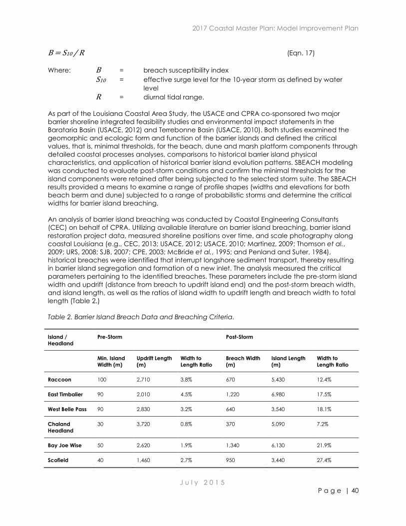
2017 Coastal Master Plan: Model Improvement Plan
J u l y 2 0 1 5
P a g e | 40
B = S10 / R (Eqn. 17)
Where: B = breach susceptibility index
S10 = effective surge level for the 10-year storm as defined by water
level
R = diurnal tidal range.
As part of the Louisiana Coastal Area Study, the USACE and CPRA co-sponsored two major
barrier shoreline integrated feasibility studies and environmental impact statements in the
Barataria Basin (USACE, 2012) and Terrebonne Basin (USACE, 2010). Both studies examined the
geomorphic and ecologic form and function of the barrier islands and defined the critical
values, that is, minimal thresholds, for the beach, dune and marsh platform components through
detailed coastal processes analyses, comparisons to historical barrier island physical
characteristics, and application of historical barrier island evolution patterns. SBEACH modeling
was conducted to evaluate post-storm conditions and confirm the minimal thresholds for the
island components were retained after being subjected to the selected storm suite. The SBEACH
results provided a means to examine a range of profile shapes (widths and elevations for both
beach berm and dune) subjected to a range of probabilistic storms and determine the critical
widths for barrier island breaching.
An analysis of barrier island breaching was conducted by Coastal Engineering Consultants
(CEC) on behalf of CPRA. Utilizing available literature on barrier island breaching, barrier island
restoration project data, measured shoreline positions over time, and scale photography along
coastal Louisiana (e.g., CEC, 2013; USACE, 2012; USACE, 2010; Martinez, 2009; Thomson et al.,
2009; URS, 2008; SJB, 2007; CPE, 2003; McBride et al., 1995; and Penland and Suter, 1984),
historical breaches were identified that interrupt longshore sediment transport, thereby resulting
in barrier island segregation and formation of a new inlet. The analysis measured the critical
parameters pertaining to the identified breaches. These parameters include the pre-storm island
width and updrift (distance from breach to updrift island end) and the post-storm breach width,
and island length, as well as the ratios of island width to updrift length and breach width to total
length (Table 2.)
Table 2. Barrier Island Breach Data and Breaching Criteria.
Island /
Headland
Pre-Storm Post-Storm
Min. Island
Width (m)
Updrift Length
(m)
Width to
Length Ratio
Breach Width
(m)
Island Length
(m)
Width to
Length Ratio
Raccoon 100 2,710 3.8% 670 5,430 12.4%
East Timbalier 90 2,010 4.5% 1,220 6,980 17.5%
West Belle Pass 90 2,830 3.2% 640 3,540 18.1%
Chaland
Headland
30 3,720 0.8% 370 5,090 7.2%
Bay Joe Wise 50 2,620 1.9% 1,340 6,130 21.9%
Scofield 40 1,460 2.7% 950 3,440 27.4%
2017 Coastal Master Plan: Model Improvement Plan
J u l y 2 0 1 5
P a g e | 41
The other critical parameter to determine is the ratio of both updrift and downdrift length to
island length. These should be greater than 27% or more from adjacent inlets. Dr. Ioannis
Georgiou of the University of New Orleans (UNO) has conducted a similar analysis of the
Chandeleur Islands, which yielded similar breaching criteria as the CEC analysis (Ioannis
Georgiou, 2014, pers. comm.).
7.3 Summary
Based on review of available literature, knowledge and experience in design and monitoring of
restoration projects along coastal Louisiana, and professional judgment, the BIMODE Team
concluded that barrier island width and width to length ratio are the primary criteria for
predicting if a breach will occur and interrupt longshore sediment transport, thereby forming a
new inlet. The following breaching criteria are applied in BIMODE each time a storm event
occurs within the simulation based on the breach data presented above:
island width = 60 m;
the ratio of both updrift and downdrift length to island length = 27%;
island width to updrift length ratio (pre-storm) = 3%; and
breach width to length ratio (post-storm) = 15%.
The critical values of island width, ratio of both updrift and downdrift length to island length,
island width to updrift length ration and breach width to length ratio are checked one by one to
determine whether a breach occurs.
The following process occurs once it is determined that a breach occurs. If the profiles do not
exceed the critical width and width to length ratios it is assumed the breach “heals” itself and
longshore transport continues. If the profiles exceed the critical width and ratio width to length
sand are greater than 27% or more from the adjacent inlets, the profiles are “turned off” and
treated as a new inlet. For additional information, refer to inlets and bays coding in Section 8.
The BIMODE Team also contemplated incorporating the geology, subsurface conditions, and
site constraints into the model; however, consensus was this would be too challenging to code
due to the number of variables including but not limited to the number of islands, geological
diversity within each region, varying subsurface conditions both in the longshore as well as the
cross-shore directions, and presence or absence of oil and gas infrastructure / canals.
2017 Coastal Master Plan: Model Improvement Plan
J u l y 2 0 1 5
P a g e | 42
8.0 Inlets and Bays
8.1 General
Barrier chains, comprising 15% of the world’s coastlines, consist of sandy islands separated by
tidal inlets that allow water and sediment exchange between the back-barrier environment and
coastal ocean (e.g., Ranasinghe et al., 2013). Tidal currents maintain a channel by removing
wave-deposited sand and building ebb- and flood- deltas seaward and landward of the inlet
throat, respectively (Hayes, 1979 and FitzGerald, 1984). Both inlet cross-sectional area and the
volume of sand comprising the ebb delta shoal positively correlate to the tidal prism (Jarret,
1976; O’Brien, 1969; and Walton and Adams, 1976). Loss of back-barrier wetlands due to rising
sea level increases tidal prism, thereby enlarging the volume of the ebb delta and dimensions of
the inlet throat (FitzGerald et al., 2008). The increasing water levels in the basin reduce frictional
damping of the tidal wave, increasing the back-barrier tidal range, which further augments the
prism (Howes et al., 2013). Increased accommodation space in the back-barrier promotes the
formation and enlargement of a flood-tidal delta. While some sand for the ebb and flood delta
enlargements comes from incision and expansion of the inlet throat, most is removed from the
adjacent barrier island shoreface littoral cells. The expanding capacity of the ebb-tidal delta in
particular may greatly diminish the amount of sand bypassing the inlet through longshore
transport, decreasing sediment supply to the downdrift barrier and hastening the transition to a
transgressive island chain (FitzGerald, 1984 and FitzGerald et al., 2008). The inference here is that
as the tidal prism increases, the capacity of the ebb-tidal delta increases and in a limited
sediment supply system, reduces bypassing because more sand goes to feed the ebb shoal.
8.2 Modeling Options
8.2.1 Inlet hydrodynamics
Inlets serve as conduits of tidal exchange between the coastal ocean and interior basins. Bruun
and Bruun and Gerritsen (1960) gave this definition for a tidal inlet, which is the most common
type of coastal inlet: “A tidal inlet is the waterway connection between the sea and a bay, a
lagoon, or a river entrance through which tidal and other currents flow.” Regardless of the inlet
origin (e.g., geologic such as the Golden Gate, hydrological where a river enters the sea, or
littoral such as openings through barrier islands), a tidal inlet must maintain sufficient velocity
through its cross section to maintain the channel of the inlet; without tidal flow the channel
closes. Knowledge of inlet hydrodynamics is critical to determining whether inlets remain open,
enlarge, or close because of insufficient current to transport sediment through the inlet. The Eco-
hydrology model used in the 2012 Coastal Master Plan modeling effort did not provide detailed
hydrodynamics, although a single velocity for every time-step is available. For example,
additional information to carry inlet stability calculations were reported by Escoffier (1940, 1977)
as well as van de Kreeke (1990), and include tidal velocities, bottom shear stress, and cross
sectional area at the inlet throat. These data can be used to estimate equilibrium shear stresses
based on knowledge or friction factors at each inlet, following methodology presented by van
de Kreeke (1990). This information is important in determining the ebb-jet size and structure, and
helping evaluate sediment transport in the vicinity of the inlet and how hydrodynamics in the
vicinity of inlets interrupt transport or alter sediment bypassing volumes (Kraus, 2000).
2017 Coastal Master Plan: Model Improvement Plan
J u l y 2 0 1 5
P a g e | 43
8.2.2 Inlet Morphology
Morphology (e.g., the cross sectional and overall shape of an inlet) is governed by several
parameters including inlet hydrodynamics and hydraulic characteristics. These include the
hydraulic radius, shape of the cross section near the inlet throat and nearby environments,
stratigraphy in the vicinity of the inlet including the depth of hard-to-erode substrate,
presence/absence of anthropogenic structures (jetties or terminal groins), relative forces of tide
versus wave dominance near the entrance, sediment supply and direction of the long shore
transport, size and shape of the ebb-tidal delta, and orientation of the inlet throat (Hayes, 1979;
FitzGerald, 1984; and FitzGerald et al., 2000). One requirement for assessing the dynamics of an
inlet’s cross-sectional area is knowledge of the tidal prism of the receiving basin. If known, then
the inlet can be adjusted using a minimum equilibrium cross section given by published
relationships (e.g., Jarret, 1976 and O’Brien, 1969), which have been modified into what is known
as the O’Brien–Jarrett–Marchi law (D’Alpaos et al., 2009). Additional models for inlet cross
sectional evolution over time using analytical methods were developed and presented by
Larson et al. (2011). The basic O’Brien relationships were implemented in the 2012 barrier
shoreline modeling with their corresponding exponents representing un-jettied Gulf coast inlets.
This includes the general form of the equation (Equation 18). Using equilibrium theory, the likely
increase in the inlet cross-sectional area is then computed using the Gulf coast version of the
Jarrett-O'Brien-Marchi relationship (D’Alpaos et al., 2009) given by:
A = kPa (Eqn. 18)
Where A = inlet cross-sectional area
k = Gulf coast coefficient
P = maximum tidal prism
a = exponent for the Gulf coast inlets.
The total tidal prism for a basin is defined as:
P = A1T1+..+AnTn (Eqn. 19)
Where P = tidal prism for the basin (estuary)
T = tidal range (m) for the nth hydrodynamic cell in the basin
A = area (open water) of the cell
n = the number of cells which make up a given bay or estuary.
The application of these relationships within BIMODE is described in Section 8.3 below.
This simple implementation however neglects complex processes such as inlet migration, which
in some Louisiana barrier islands can be important through the course of 25 to 50 years (Miner et
al., 2009a and Miner et al., 2009b). Levin (1993) presented a classification scheme of Louisiana
inlets, on the basis of previous work by Hubbard et al. (1979), which recognized wave, tidal or
mixed morphology inlets. This approach however only approximately describes the planform
and submerged morphology qualitatively. Using an in-depth analysis of tidal prism and inlet
geometry, Howes et al. (2013) presented more specific quantitative metrics to classify inlet
morphology on the basis of additional hydraulic characteristics and namely the hydraulic radius.
The methodology proposed here, although simple, is very powerful and can be implemented
immediately. Although the omissions appear significant, their relative contribution to inlet
morphology is rather small compared to the dominant effect of the tidal prism, which is already
2017 Coastal Master Plan: Model Improvement Plan
J u l y 2 0 1 5
P a g e | 44
addressed. Furthermore, there is limited information to describe these additional dynamic
process associated with inlet evolution, and collecting more data to develop relationships that
better constrain first order response was not achievable within the time frame of this effort.
8.2.3 Interaction of Inlets with Nearby Environments
Obviously, since inlets connect the coastal ocean and interior bays, any model used to assess
this interaction must be at least able to force exchange caused by pressure gradients across the
inlet. Most models, including the Eco-hydrology model developed for the 2012 Coastal Master
Plan, can already address this. This computation is critical for calculating tidal prism.
Inlets are often associated with ebb (and/or flood) deltas or shoals. Knowledge of ebb delta
morphology and dimensions is critical for correctly interpreting processes in the nearshore
environments near barriers. For example, sediment bypassing is a process associated with inlets;
however, ebb deltas often control the temporal and spatial aspects of sediment bypassing inlets
and impose additional sediment sinks/sources that could significantly affect the longshore
sediment transport budget. FitzGerald et al. (2000) suggested natural mechanisms for sediment
bypassing at tidal inlets. Their study, supplemented by additional data from previous research,
concluded that the governing variables for sediment bypassing include tidal prism, inlet
geometry, wave and tidal energy, sediment supply, spatial distribution of back-barrier channels,
regional stratigraphy, slope of the nearshore, and engineering modifications (if present). Kraus
(2000) extended this work further to develop a quantitative tool for ebb-shoal evolution and
sediment bypassing at inlets. This mathematical model calculates the change in volume and
sand-bypassing rate at ebb-tidal shoals. This is done by distinguishing bypassing bars from
attachment bars, allowing for the transfer of sediment across the distal ebb-delta (shoal) (Figure
6). The volumes and bypassing rates of these morphologic entities are calculated by analogy to
a reservoir system, where each reservoir can fill to a maximum (equilibrium) volume. The ratio of
the input longshore sand transport rate and the equilibrium volume of the morphologic feature is
found to be a key parameter governing morphologic evolution. The model was validated with
observations in Ocean City inlet, Maryland, and used to test deviation in sediment bypassing
volumes as a result of mining of the ebb-shoal through a hypothetical idealized scenario.
While the reservoir model presented in Kraus (2000) is robust and easy to implement, the data to
validate this model along all inlets in coastal Louisiana is lacking. In Louisiana, there are several
inlets (e.g. Coupe Colin, Whiskey Pass, Little Pass Timbalier) that are not well defined; they are
transgressive systems and tend to be wave influenced and storm-dominated. These inlets are
especially important for several reasons. First, although they are rather large inlets (3-5 km
across), they have a narrow active channel and thalweg (1-2 km) and are flanked on one or
both sides by a shallower subaqueous platform. The flow dynamics of the thalweg and adjacent
platform areas have significant influence on sediment transport (both longshore and cross-
shore), something that can critically affect barrier island evolution as well as the evolution of the
ebb-delta. This made application of a reservoir type model difficult, without additional data to
calibrate and validate. Thus the reservoir model (Kraus, 2000) was not recommended for
utilization in BIMODE.
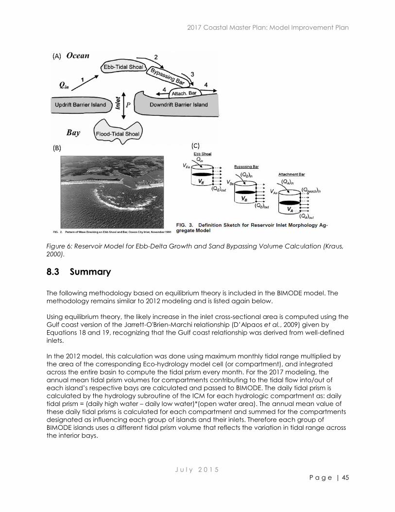
2017 Coastal Master Plan: Model Improvement Plan
J u l y 2 0 1 5
P a g e | 45
Figure 6: Reservoir Model for Ebb-Delta Growth and Sand Bypassing Volume Calculation (Kraus,
2000).
8.3 Summary
The following methodology based on equilibrium theory is included in the BIMODE model. The
methodology remains similar to 2012 modeling and is listed again below.
Using equilibrium theory, the likely increase in the inlet cross-sectional area is computed using the
Gulf coast version of the Jarrett-O'Brien-Marchi relationship (D’Alpaos et al., 2009) given by
Equations 18 and 19, recognizing that the Gulf coast relationship was derived from well-defined
inlets.
In the 2012 model, this calculation was done using maximum monthly tidal range multiplied by
the area of the corresponding Eco-hydrology model cell (or compartment), and integrated
across the entire basin to compute the tidal prism every month. For the 2017 modeling, the
annual mean tidal prism volumes for compartments contributing to the tidal flow into/out of
each island’s respective bays are calculated and passed to BIMODE. The daily tidal prism is
calculated by the hydrology subroutine of the ICM for each hydrologic compartment as: daily
tidal prism = (daily high water – daily low water)*(open water area). The annual mean value of
these daily tidal prisms is calculated for each compartment and summed for the compartments
designated as influencing each group of islands and their inlets. Therefore each group of
BIMODE islands uses a different tidal prism volume that reflects the variation in tidal range across
the interior bays.
2017 Coastal Master Plan: Model Improvement Plan
J u l y 2 0 1 5
P a g e | 46
9.0 Aeolian Processes
9.1 General
The liberation, transport and consequent deposition of sand by wind-driven processes occurs
when sediment is available and sufficient strength winds are present (Kok et al., 2012). Along
sandy coastal barrier systems aeolian processes are a mechanism of sediment transfer from the
beach to supratidal dune systems and dune systems into lower tidal elevations such as the
beach face and nearshore (Ritchie and Penland, 1990). Sediment transport by wind is a highly
dynamic process that can result in the temporary (transport into the littoral zone) or longer time
scale (fully developed supratidal dune fields) sequestration of sediment across a range of barrier
shoreline environments.
The median grain size of Louisiana sandy barrier headlands and barrier island systems falls within
the fine sand range of 0.09 mm to 0.14 mm (Campbell et al., 2005). This sediment class can
readily be moved by aeolian forces and summer thunderstorm activity; tropical cyclones and
pre-frontal south winds that accompany the passage of winter cold fronts and post-frontal north
winds all generate sustained wind velocities that are capable of silt and sand transport along
the Louisiana coast through suspension, saltation, or bed surface creep.
The depositional patterns and magnitude of aeolian transported sediment are however very
poorly understood along the Louisiana coastal zone and adequate data do not currently exist
to provide a calibrated numerical model of aeolian sediment movement. However, aeolian
transport science does provide several methods and approaches to the calculation of aeolian
sediment transport.
9.2 Model Options
There exists a variety of approaches to calculating sediment flux by wind driven transport. In
general the existing quantitative approaches rely fundamentally on knowledge of wind speed,
median grain size, and air density (variable by humidity) to determine critical values allowing for
aeolian sediment motion.
9.2.1 Bagnold Method
According to the Bagnold equation (1941), the discharge of sediment in kg/s/m width is:
𝑞 = 𝐶 (𝑑
𝐷)
0.5
(𝜌𝑎
𝑔) 𝑈∗
3 (Eqn. 20)
Where: q = sediment discharge (kg/s/m)
𝐶 = a constant equal to 1.8 for dune sand
𝑑 = mean grain size diameter
𝐷 = reference grain size of 0.25 mm
𝑔 = acceleration due to gravity
𝜌𝑎 = air density
𝑈∗ = shear velocity (m/s).
2017 Coastal Master Plan: Model Improvement Plan
J u l y 2 0 1 5
P a g e | 47
For the temperature range of -10º C to 50º C, errors in air density due to humidity are less than
0.2%. Therefore, the effects on air density due to humidity can be ignored (Masamichi et al.,
2008). The value for shear velocity, 𝑈∗, can be found with the equation:
𝑈∗ = 0.4 [𝑈5𝑚
𝑙𝑜𝑔(5
𝑍0)] (Eqn. 21)
Where: 𝑈5𝑚 = wind speed at 5 m
𝑍0 = roughness length (assumed to be 0.02m).
Subsequently, Bagnold formulated a different equation for estimating q in metric tons/hr/m
width:
𝑞 = 5.2 × 10⁻⁴(𝑈 − 𝑈𝑐)3 (Eqn. 22)
Where: q = sediment discharge (metric tons/hr/m)
𝑈 = wind speed in cm/s at 1 m above the ground surface
𝑈𝑐 = threshold velocity of 400 cm/s.
9.2.2 Hsu Method
Hsu (1974, 1987) formulated relationships connecting sediment transport to the Froude number
given by the following equations:
𝑞 = 𝐻 [𝑈∗
(𝑔𝑑)0.5]3
(Eqn. 23)
Where: 𝑑 = mean grain size diameter (cm)
𝑈∗ = shear velocity (cm/s)
𝑔 = accleration due to gravity (cm/s2)
𝐻 = aeolian sand transport coefficient with same dimensions as q
(g/cm-s) and can be found with the relationship:
ln(𝐻) = (−0.42 + 4.91𝑑𝑙𝑜𝑤𝑒𝑟) × 10−4 (Eqn. 24)
Where: 𝑑lower = grain size (mm).
For dry beaches, Hsu (1974, 1987) created a relationship between wind speeds at a height of 2
m and the shear velocity given by the following equation:
𝑈2𝑚,𝑡 =𝑈∗𝑡
0.044 (Eqn. 25)
Where: 𝑈2𝑚,𝑡 = threshold wind speed at height of 2 m
𝑈∗𝑡 = threshold shear velocity.
2017 Coastal Master Plan: Model Improvement Plan
J u l y 2 0 1 5
P a g e | 48
Manipulation of drag coefficient equations yields the formula:
𝑈5𝑚,𝑡 =[𝑈∗t𝑙𝑛(
𝑍2𝑍1
)]
𝑘+ 𝑈2𝑚,𝑡 (Eqn. 26)
Where: 𝑈5𝑚,𝑡 = threshold wind speed at height of 5 m
z2 = anemometer height of wind speed measurements
z1 = 2 m (from Hsu’s relationship)
𝑘 = von Karman’s constant (0.4).
Wind speeds exceeding this value of 𝑈5𝑚,𝑡 are able to transport sediment, whereas velocities
smaller than the threshold wind speed are assumed to have a transport rate of zero. If 𝑈5𝑚 > 𝑈5𝑚,𝑡 the following equation is applied to find the shear velocity:
𝑈∗ = 0.044 𝑈5𝑚 (Eqn. 27)
Where: U5m = wind speed at 5 m and should be converted to cm/s to produce a
𝑈∗ value (cm/s).
To calculate the sediment transport rate, a formula by Hsu (1987) states:
𝑞 = 𝐾 [𝑈∗
(𝑔𝑑)0.5]3
(Eqn. 28)
Where: 𝑞 = sediment transport rate (g/cm-s)
𝑔 = accleration due to gravity (cm/s2)
𝑈∗ = shear velocity (cm/s)
𝑑 = median grain size diameter (cm)
𝐾 = dimensional aeolian transport coefficient with the same
dimensions as 𝑞 and calculated by:
𝐾 = 𝑒−9.63+4.91𝑑 (Eqn. 29)
Where: 𝑑 = median grain size diameter (mm), regardless of the units of K.
This equation for K cannot be applied if the mean grain size diameter exceeds 1.0 mm.
9.2.3 CEM Method
The Coastal Engineering Manual (CEM) (USACE, 2002) employs a method of calculating
transport rates based primarily on Bagnold (1936, 1941) and Hsu (1974, 1987) transport rate
equations. The CEM method first calculates the threshold wind speed or the wind speed
required to initiate the movement of sand particles. This critical shear stress (or threshold wind
speed) is provided by Bagnold (1941) with the equation:
𝑈∗t = 𝐴𝑡 {[(𝜌𝑠−𝜌𝑎)𝑔𝑑]
𝜌𝑎}
0.5
(Eqn. 30)
2017 Coastal Master Plan: Model Improvement Plan
J u l y 2 0 1 5
P a g e | 49
Where: At = a dimensionless constant equal to 0.118
𝜌𝑠 = sediment’s mass density
𝜌𝑎 = air density
𝑔 = acceleration due to gravity (m/s2)
𝑑 = the lower limit grain size diameter (m).
This equation yields a threshold velocity in m/s for the dimensions specified.
The final step of the CEM Method requires the determination of a volumetric transport rate from
the mass transport rate, indicating
𝑞𝑣 =𝑞
[𝑝𝑠(1−𝑝)] (Eqn. 31)
Where: 𝑞𝑣 = volumetric transport rate (cm3/cm-s)
𝑞 = sediment transport rate (g/cm-s)
𝑝𝑠 = sediment mass density (g/cm3)
𝑝 = porosity of the in situ sand (assume = 0.4).
This volumetric transport rate can be converted to m3/m-s if multiplied by 10-6 and tons/hr/m if
multiplied by 0.360.
9.3 Summary
Though these types of quantitative approaches provide estimates of aeolian transport, there
exists a fundamental lack of parameters and data for the Louisiana sandy shoreline to
effectively model aeolian transport patterns and sediment volumes.
First, there exists a wide range of variability in the average wind speed, wind patterns, and
frequency of events that can generate velocities capable of aeolian sediment transport. In the
absence of wind climate with good spatial and temporal variability, predicted rates would likely
be unrealistic. Furthermore, information on the wind boundary layer is lacking and hence correct
estimations of shear velocity are not achievable.
Second, there has been no comprehensive inventory of the sediment properties and
characteristics of dune systems along Louisiana sandy barrier shorelines since the late 1980’s to
early 1990’s (e.g., Ritchie, 1989 and Ritchie, et al., 1992). Consequently, there currently exists no
fully compiled and current inventory of dune characteristics or the types of morphologic
responses that Louisiana coastal dune systems have undergone in response to overwash
processes and winds by which to calibrate and validate quantitative aeolian models.
Finally, information and data that are required to correctly characterize lag effects after storms
associated with sand transport are limited. For instance, post-storm, formerly subaerial sand is
often supply limited and stored offshore. Lag effects associated with the introduction of sand first
into the littoral zone, then onto a deflated berm is also lacking, making modeling of these
processes extremely challenging.
Based on the lack of data (e.g., wind boundary layer, inventory of dune characteristics and their
types of morphological responses, and lag effects after storms), the BIMODE Team considered it
2017 Coastal Master Plan: Model Improvement Plan
J u l y 2 0 1 5
P a g e | 50
unreasonable to attempt incorporating aeolian transport equations into the BIMODE model.
There is value however in considering that aeolian transport may play a positive role in barrier
island longevity and supratidal elevation gain following barrier renourishment efforts when
sufficient sand is available to the system, and several Louisiana barrier island restoration projects
have incorporated aeolian concepts into renourishment engineering. For degraded barriers with
limited sediment supply there appears to be no net benefit to the placement of dune fencing.
The 2017 Coastal Master Plan vegetation modeling team evaluated minimum elevations for the
barrier island vegetated dune communities. Based on their evaluation (Jenneke Visser, 2012,
pers. comm.), they established that dune vegetative species occur at the first point traveling
landward of the Gulf where the elevation equals 0.698 m above mean sea level. Based upon
the knowledge, experience, and professional judgment of the BIMODE Team, this is a
conservative estimate and will support dune vegetation in the wake of significant storm impacts
and overwash.
2017 Coastal Master Plan: Model Improvement Plan
J u l y 2 0 1 5
P a g e | 51
10.0 Post-Storm Recovery
10.1 General
In the context of BIMODE, post-storm recovery is defined as the return of sediment (which was
eroded during the storm) to the barrier island that contributes to the re-establishment of its
geomorphic form and ecologic function from natural processes. Recovery of the barrier islands
in the wake of significant storm events has been documented in the literature, e.g., Kahn (1986),
Fearnley et al. (2009), and Martinez et al. (2009). These historical analyses demonstrate recovery
periods whereby the shorelines accrete or experience less severe erosion compared to storm
periods.
Dingler and Reiss (1995) reported that Hurricane Andrew, which passed directly over Isles
Dernieres in 1992, stripped all the sand from Trinity Island’s beach face, exposing the underlying
mixed sediment core. It was estimated that the impact of the storm resulted in approximately 90
m of berm crest migration to the north and a sediment loss of approximately 80 m3/m from the
shoreline. Observations conducted one year after the hurricane’s passage indicated the core
remained exposed and the upper foreshore eroded over 24 m.
Stone et al. (2007) examined the impacts of Hurricanes Andrew (1992), Lili and Isidore (2002) and
Katrina and Rita (2005), which all caused significant damages to the barrier islands within the
study area. They reported that while post-storm recovery does occur, it is very slow and the multi-
decadal increase in both storm frequency and intensity is resulting in a net loss in the overall
sediment budget.
Fearnley et al. (2009) and Sallenger et al. (2009) analyzed the recovery potential of the
Chandeleur Islands in the wake of Hurricanes Katrina and Rita that adversely impacted these
islands in 2005. It was estimated that 86% of the surface area of the Chandeleur Islands was
eroded by Hurricane Katrina. Immediate post-storm observations revealed that all of the sand
visible from the air was removed, leaving only marshy outcroppings. Analyses of aerial
photography taken two months after the storm concluded the islands were still rapidly eroding
after the storm noting Hurricane Rita impacted the area during this time frame causing some of
the erosion.
10.2 Model Options
Based upon the literature review, no industry standard empirical or theoretical numerical models
exist to predict post-storm recovery of the barrier islands. The cross-shore model Beach-fx
includes a post-storm recovery factor of 70% to 80% of the beach berm width (Mark Gravens,
2013, pers. comm.). As described in Section 6, this model was not recommended for the BIMODE
model as it does not allow for certain processes that are viewed as essential for modeling the
behavior of the barrier islands of Louisiana.
Knowledge and experience from restoration project design (e.g., CEC and SJB, 2008; USACE
2010; and USACE, 2012) indicates the SBEACH model under-predicts the amount of erosion and
overwash due to storm events, and upon examining the islands and their recovery period, the
SBEACH predictions more closely match the net change, that is, the combination of storm
erosion and recovery.

2017 Coastal Master Plan: Model Improvement Plan
J u l y 2 0 1 5
P a g e | 52
10.3 Summary
The SBEACH model was the preferred model for the cross-shore processes, and experience has
indicated that SBEACH tends to under predict storm erosion, which in some sense accounts for
post-storm recovery processes. Accordingly, the BIMODE Team suggests the post-storm recovery
processes are captured sufficiently through application of SBEACH.

2017 Coastal Master Plan: Model Improvement Plan
J u l y 2 0 1 5
P a g e | 53
11.0 Subsidence
11.1 General
Subsidence is the gradual sinking or lowering of the land surface. It is one of the key physical
processes affecting landforms within the focus area. With respect to coastal Louisiana, six
primary processes cause subsidence (Reed and Yuill, 2009) including:
Tectonic subsidence;
Holocene sediment compaction;
Sediment loading;
Glacial isostatic adjustment;
Fluid withdrawal; and
Surface water drainage and management.
CPRA convened a panel of experts in 2010 to examine the causes of subsidence, review existing
literature on historic subsidence rates, assess procedures for predicting subsidence, and render
recommendations for future planning purposes including the 2012 Coastal Master Plan. The
outcome of the panel’s recommendations included a spatially defined map representing
plausible ranges of subsidence over the next 50 years. The ranges of subsidence rates for coastal
Louisiana are shown in Figure 7 and listed in Table 3 specific to the study area (CPRA, 2012). It is
noted these ranges do not include ESLR or the compaction due to loading from future projects.
These physical processes are addressed separately.
11.2 Application for BIMODE
Guidance from CPRA was to follow the same procedure for applying the effects of subsidence
on barrier island evolution utilized in the 2012 Coastal Master Plan for coding and testing of the
BIMODE model.
The barrier shoreline morphology model developed for the 2012 Coastal Master Plan accounted
for the effects of subsidence through application of a simple one-dimensional relationship
wherein the elevations along the cross-shore profile were lowered by the subsidence rate (Figure
8). Spatially variable subsidence was applied with one set of values applied for the moderate
future scenario and one set of values for the less optimistic future scenario. For the moderate
and less optimistic projections, CPRA utilized professional judgment to select the lower 20th
percentile and 50th percentile of the plausible ranges of future subsidence rates, respectively, for
each region (CPRA, 2012). The values applied for the study area are presented in Table 3.
The BIMODE model can updated if needed and future efforts will be coordinated with the
broader 2017 Coastal Master Plan modeling effort.
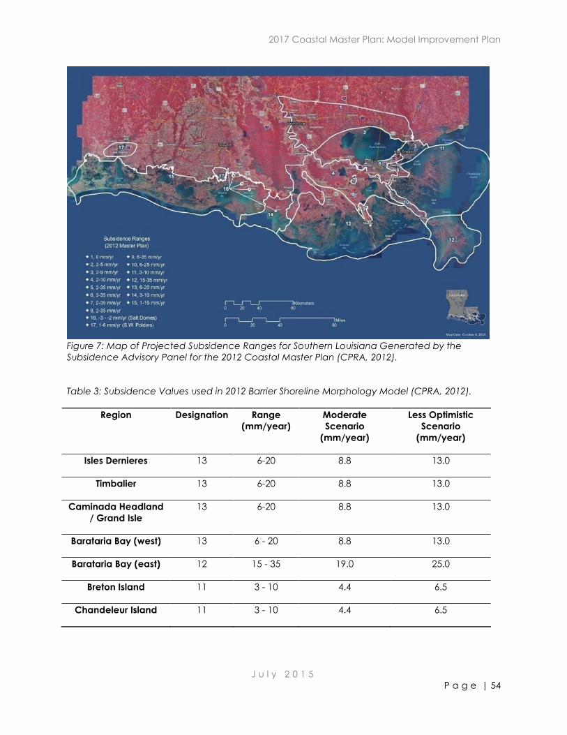
2017 Coastal Master Plan: Model Improvement Plan
J u l y 2 0 1 5
P a g e | 54
Figure 7: Map of Projected Subsidence Ranges for Southern Louisiana Generated by the
Subsidence Advisory Panel for the 2012 Coastal Master Plan (CPRA, 2012).
Table 3: Subsidence Values used in 2012 Barrier Shoreline Morphology Model (CPRA, 2012).
Region Designation Range
(mm/year)
Moderate
Scenario
(mm/year)
Less Optimistic
Scenario
(mm/year)
Isles Dernieres 13 6-20 8.8 13.0
Timbalier 13 6-20 8.8 13.0
Caminada Headland
/ Grand Isle
13 6-20 8.8 13.0
Barataria Bay (west) 13 6 - 20 8.8 13.0
Barataria Bay (east) 12 15 - 35 19.0 25.0
Breton Island 11 3 - 10 4.4 6.5
Chandeleur Island 11 3 - 10 4.4 6.5
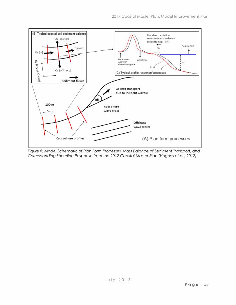
2017 Coastal Master Plan: Model Improvement Plan
J u l y 2 0 1 5
P a g e | 55
Figure 8: Model Schematic of Plan Form Processes, Mass Balance of Sediment Transport, and
Corresponding Shoreline Response from the 2012 Coastal Master Plan (Hughes et al., 2012).
2017 Coastal Master Plan: Model Improvement Plan
J u l y 2 0 1 5
P a g e | 56
12.0 Eustatic Sea Level Rise
Relative sea-level refers to the height of sea level as measured from a particular point or area on
the earth's surface. The National Research Council (NRC) (1987) initially developed an equation
and values to estimate relative sea level rise (RSLR) which is the combination of ESLR and
subsidence. The USACE (2009, 2011) updated this equation and shifted the base year from 1987
to 1992. The Intergovernmental Panel on Climate Change (IPCC) developed SLR trends based
on recent climate research (IPCC, 2007).
For the 2012 Coastal Master Plan, the plausible range of sea level rise over 50 years utilized a low
boundary of 3.1 mm/yr equal to 0.155 m over 50 years taken from IPCC (2007), and a high
boundary assuming an acceleration of 1.005 x 10⁻⁴ consistent with NRC (1987) and USACE (2009)
equal to 0.65 m over 50 years. Moderate and less optimistic projections were chosen for the
landscape models and were determined utilizing the generalized equation for SLR given by:
𝐸 (𝑡2 − 1986) − 𝐸(𝑡1 − 1986) = 𝑎([𝑡2 − 1986] − [𝑡1 − 1986]) + 𝑏([𝑡2 − 1986]2 − [𝑡1 − 1986]2)
(Eqn. 32)
Where: 𝐸 = change in ESLR at time t 𝑎 = historical linear rate of global SLR = 0.0031
𝑏 = acceleration constant for predicted global SLR
= 2.36 x 10⁻⁵ (moderate) and 6.2 x 10⁻⁵ (less optimistic) (CPRA, 2012).
CPRA will provide updated projections for use in the 2017 modeling. The BIMODE model will be
updated accordingly, and future efforts will be coordinated with the broader 2017 Coastal
Master Plan modeling effort.
2017 Coastal Master Plan: Model Improvement Plan
J u l y 2 0 1 5
P a g e | 57
13.0 Model Schematization
This section discusses the schematization of the BIMODE model and outlines how the selected
physical processes are incorporated to develop the final output.
Step 1. Establish littoral cells. Create profiles from available data. Convert x,y,z data into profile
based data. Determine azimuth for each profile and store so that profile data can be
converted back to x,y,z format.
Step 2. Prepare input parameters for each profile including silt content, initial active profile
height, and post-restoration profile. Data is included as a look-up table.
Step 3. Select wave climate for period between storm events. Select an appropriate WIS
hindcast station for the barrier island domain of interest. Transform the full 33-year WIS
time series from the hindcast station to the offshore depth of the SWAN grid using the
WIS Phase 3 transformation technique and specifying the regional shoreline orientation
and sheltering angles as appropriate. Then, the transformed time series is parsed by
month in preparation for performing the monthly statistical characterization. The time
series is grouped by specified angle bands and period bands. The monthly statistical
analysis results in the identification of a limited number of "characteristic" wave
conditions for each month. The monthly wave data series are provided as input for
BIMODE on a monthly time step.
Step 4. Develop a database of nearshore wave conditions for each of the model segments
(transects) by transforming waves from offshore location to a depth contour before
breaking (-6 foot contour suggested) using SWAN. This process contains both offshore
wave transformation (WIS Phase III) and nearshore wave transformation before
breaking. Select representative monthly wave data and create a look-up table for
each offshore wave condition to output a nearshore wave condition. The last part of
wave transformation to wave breaking is performed within BIMODE. The wave height,
period and direction at breaking location are used for longshore sediment transport.
This step is only performed once using existing available bathymetry. It is assumed that
the impact of relative sea level rise on wave transformation is minimal compared to
other modeled processes.
Step 5. Develop look-up tables for cross-shore storm model runs. For proof of concept, 1008
runs were performed as described in Section 14.0 (7 storm events run on 6 different
profile lines with 24 different cross-sections). Look-up tables are either based on cross-
shore profile or a tabulation of retreat of various contours along the beach face and
tracking of overwash distance on the bay side.
Step 6. Check whether the profile still has a subaerial component. If yes, then continue; if not,
then move to next profile and repeat Step 6.
Step 7. Compute longshore transport rate from each of the monthly representative wave
conditions for each emergent profile for the given time interval. Read local wave
height, period and direction at each timestep of the wave record using wave
transformation from Step 4. Determine longshore transport rate based on the CERC
equation for sediment transport. Calculate cumulative longshore gross transport values
(e.g. sum of easterly transport and sum of westerly transport) as well as net sediment
transport and direction for the month. Repeat for all months in the year.
2017 Coastal Master Plan: Model Improvement Plan
J u l y 2 0 1 5
P a g e | 58
Step 8. Locate divergence of sediment transport within each littoral cell (nodal point). Variable
nodal points are calculated. Sum net transport rates changes going away from the
nodal point to determine erosion or accretion at each profile line. Check whether the
profile is adjacent to a pass such that gross transport into the pass is lost from system.
(Alternate option is to sum transport loss to the pass and estimate whether subaerial
growth could occur).
Step 9. Change beach face profile location by equating sediment transport loss or gain to
shoreline retreat or advance. Read in active profile height from profile (probably fix
depth of closure specific to each region and then read either dune crest or estimate
berm elevation from cross-section). (Volume = Distance between profiles times active
profile height times change in shoreline location.)
Step 10. Account for profile elevation adjustments due to sea level rise and subsidence in given
time period. Read in sea level rise from a table to account for variability with time.
Read in subsidence and/or primary consolidation due to project construction to
account for variability with time. Adjust elevations of points along beach profile to
account for consolidation.
Step 11. Account for silt loss. Increase the shoreline retreat by the percentage of silt in the
beach face.
Step 12. Combine shoreline changes due to longshore transport and silt loss. Retreat the beach
face profile by the combined change.
Step 13. Reduce elevation of each point along the cross-section uniformly to account for
subsidence. (Detritus can be added to the subsidence value either implicitly or
explicitly as its own table. The value would be included in this step.)
Step 14. Repeat Step 9 through Step 13 for each profile.
Step 15. Is a storm predicted within this time period? If no, then skip to Step 20. If yes, then
determine profile values for berm width, dune height, and dune width. Access the look-
up table to find the input profile that most closely matches these values and the storm
event that most closely matches the specified storm. Overwrite the input profile with
the post-storm profile from the look-up table. Use the seaward high tide line to locate
the profile. This step accounts for the storm-induced shoreline change due to cross-
shore sand transport. Overwash beyond the marsh platform is also encompassed in the
SBEACH look-up tables. (This may be changed to track only a few contours and
develop a look-up table for the retreat of those contours.)
Step 16. Repeat for all profiles.
Step 17. Is another storm predicted in this time period and can longshore processes be
excluded between storm events? If so, return to Step 16.
Step 18. Smooth the shoreline.
Step 19. Erode the bayward side of the profile if applicable. This is based on the marsh edge
erosion subroutine of the ICM.
2017 Coastal Master Plan: Model Improvement Plan
J u l y 2 0 1 5
P a g e | 59
Step 20. Check whether each island exceeds the island breaching thresholds. The first step is to
determine profiles with island width less than 60 m, which can potentially breach. Then
confirm the potential breach is far-field from island ends (the ratio of both updrift and
downdrift length to island length are 27% or more from adjacent inlets). The other
criterion is to check for the critical width to updrift length ratio. If the ratio is less than
3%, the island can potentially breach. For the profiles with both of the criteria satisfied,
the breach is initiated. If the breaching thresholds are exceeded, determine which
profiles are most likely to breach and label the number of consecutive profiles equal to
the critical width as being submerged (no longshore transport). Reset the definition of
island for subsequent breach evaluations.
Step 21. Incorporate the inlet and bay module at the specified time step. One-year intervals are
currently preferred.
Return to Step 6 and repeat until 50-year simulation period is complete.
Output is a cross-section at each emergent profile in the format of a DEM.
For the future with project scenarios, BIMODE has the ability to input a restoration project in the
50-year simulation or add renourishment of a previously restored island at a specific target year.
The goal is to automate this procedure; however, it is understood that the design template will
have to be positioned in relationship to the island position at the specified target year noting the
landward migration of the barrier islands due to overwash and other erosional processes. The
details of this are currently in progress.

2017 Coastal Master Plan: Model Improvement Plan
J u l y 2 0 1 5
P a g e | 60
14.0 BIMODE Code Development & Testing
14.1 Overview
This section describes the routines developed to simulate the steps outlined in the previous
Model Schematization section and the quality control testing performed to confirm the
functionality and accuracy of the program. The code in its entirety was submitted to CPRA (as
Appendix 2).
14.2 BIMODE Code
The BIMODE code was written in Fortran 90. It consists of a single main program, BIMODE.f90,
which calls on an input file, a global variable file and several subroutines to perform the
necessary computations. The format of the input and output for the program is an ASCII grid file
in .XYZ format and a text file with input/ output parameters. The datum of the input and output
files is in Universal Transverse Mercator (UTM) 15 coordinates in meters. The elevation datum is
NAVD 88 (Geoid ’09) in meters.
14.2.1 File Structure
The BIMODE code requires the following files to run:
BIMODE.f90 is the main program file. It calls the input file, variable file, and subroutines
necessary to run the program.
Mod_global.f90 defines the parameters necessary for computation i.e. gravity,
sediment density, density of water and coefficients in the CERC equation. It also
allocates variables for assignment in the subroutines.
The file mod_util.f90 provides utility to read input and is only used in subroutine
“read_input” in the following section.
Input.txt is the input parameter file for the program. It governs the start and end time
of the model, the grid spacing, the profile naming, reading the wave data look-up
table, reading the SBEACH look-up table and the input parameters. The input
parameters include sea level rise rate, subsidence rate, silt content, breaching
criteria and marsh erosion rate.
Excel_Date_Table_1900to3100.txt is the date code file starting from 1900 to 3100. All
the time points in BIMODE are expressed in terms of days according to this file.
Storm_event.prn is a text file listing the storm occurrences for the simulation. Time of
occurrence is set as Year, Month, Day, Hour and Minute that a storm is to occur
during the simulation.

2017 Coastal Master Plan: Model Improvement Plan
J u l y 2 0 1 5
P a g e | 61
The SBEACH look-up table is stored in SBEACH.tab. This table contains the initial pre-
storm profiles and the post-storm transformation correlated to storm event and initial
profile.
The wave look-up table is stored in WIS_station_name_WIS.tab (for example
ST73141_WIS.tab). There were four WIS stations selected to develop the average
wave climate. Each wave case contains the significant wave height, wave period,
wave direction and the depth.
The wave time series from each WIS station is saved as
WIS_station_name_WIS_reformat.prn (for example ST73141_WIS_reformat.prn).
A survey file in.XYZ format contains profile number, coordinates (x,y) and elevation (z)
and is required to run the program.
A survey control file in control.prn contains the starting coordinates and profile
azimuth.
14.2.2 Main Subroutines
The first step in running BIMODE is to read the input file, .XYZ data file, survey control file, look-up
tables, storm event control file and wave time series, using subroutine “read_input.” This
subroutine calls on the file mod_util.f90 to read and format the input file parameters.
Next, the subroutine “allocate_variables” is called to allocate space for and assign initial values
to the variables in all of the other subroutines. The program then checks for subaerial points
along each profile, using “check_subaerial.” A subaerial point was defined as any point with an
elevation above 0 meters NAVD88.
The following subroutine, “check_island,” is used to determine if the profile aligns with an island.
An island has seaside submerged points and bayside submerged points. If an island does exist,
the island width is calculated for use later for breaching criteria. The island width is defined as
the distance from the seaside zero-contour to the northern-most zero-contour. Note that the .XYZ
data file may contain missing data points. In order to eliminate all missing points, LIDAR data are
applied first; then, linear interpolation is performed to fill in the remaining missing points. If LIDAR
data is applied, the program smoothes the cross-shore profile data based on a 21 point
smoothing algorithm.
To compute the final wave transformation from the nearshore to the breaking point, the
subroutine “wave_transform” is run. The wave height, wave period and wave direction are read
in from wave data look-up table. The look-up table contains wave data developed from the
Hypercube analysis of the WIS data for each WIS station. In the Hypercube analysis, the wave
transformation is performed for a number of wave cases with various height bands, period
bands and direction bands. Then the 3D linear interpolation is used to obtain the wave
refraction coefficients for any other wave cases. The WIS data record extended from January 1,
1980 to December 31, 2012 (33 years). In order to complete a 50-year simulation, the wave
record was repeated, providing 66 years of data.
2017 Coastal Master Plan: Model Improvement Plan
J u l y 2 0 1 5
P a g e | 62
The subroutine “longshore_transport” is used to calculate longshore transport by waves based
on CERC (1984). First, the cumulative longshore gross transport rate is calculated. The direction of
transport depends on the wave angle. Then, the net transport at each cell (area between
profiles) is calculated. The net longshore transport is smoothed across profiles using the inverse-
distance weighted method (Lam, 1983). For each target profile, the smoothed net longshore
transport is weighted by transports at both the target profile and the adjacent profiles. The
further profile from the target profile makes less contribution to the transport. This avoids a
feedback loop in the model because shoreline change affects wave angle and thus drives
further change.
The following three subroutines calculate shoreline retreat rates and update the profiles. The
subroutines below are applied after longshore transport at each time step (monthly).
“silt_loss”: accounts for silt loss based on silt content (Default is 0.3)
“sea_level_rise”: calculates sea level rise rate as a function of time
“land_subsidence”: calculates land subsidence, affects entire profile.
The subroutine “crossshore_transport” updates the profiles based on storm-induced cross-shore
transport applied by referencing the transformations stored in the SBEACH look-up table. The
program knows a storm occurs based on the sequence of storm events saved in the
storm_event.prn file. When a storm occurs, the program compares the existing profile to the
idealized initial profiles stored in the SBEACH look-up table. The middle point of the maximum
dune height of the idealized profile is aligned over the existing profile for comparison. Then, the
program selects the idealized profile with the minimum difference from the existing profile. Based
on this selected idealized profile and the given storm event, the SBEACH look-up table is used to
identify the profile transformation that was simulated in SBEACH (outside of BIMODE) to occur.
Hundreds of idealized profiles with maximum dune heights that vary by 0.1 meters and varying
dune widths were simulated in SBEACH with varying return period storms to provide data for the
SBEACH look-up table. Finally, the profile transformation is applied to the active portion of the
existing profile and a post-storm profile is generated inside BIMODE.
The shoreline position is updated at each time step by the “update_shoreline” routine. Based on
profile changes, the seaside shoreline either advances or retreats. The bayside shoreline is also
updated but as a result of the marsh erosion function.
The “check_breaching” subroutine is used to check the breaching threshold of an island based
on two criteria: barrier island width and the island width to length ratio. The critical values of
these criteria were set as constants in the code. The critical width (less than 60 m) is firstly
determined among all the profiles. The potential breach is far-field from island ends, which is 27%
or more from adjacent inlets. The critical width to updrift length ratio is set as 3%. In general, for
the profile that is less than 60 m wide from gulf mean high water to bay mean high water, is
located greater than 27% of the total island length from both adjacent inlets, and its width to
updrift length ratio is less than 3%, a breach is initiated.
The subroutine “write_output” generates the output files. The first output file is the XYZ file
(Profile_0001), which contains the final profile data. Next, the text file containing the cumulative
longshore transport is generated Qsum_0001. Finally, a time series of shoreline retreat and
advance is printed, time_series.txt. At the same time, a running log file is generated during the
calculation.

2017 Coastal Master Plan: Model Improvement Plan
J u l y 2 0 1 5
P a g e | 63
There are other subroutines and functions in the program to support the functions of the main
subroutine. These subroutines include:
Gmt2datecode: converts date and time from input.txt into a time table date number.
Exist_error: prints error messages if necessary while reading input file data.
Several linear interpolation methods based on nearest points.
Solv_disprsn: solves dispersion equation for wave length using the Newton-Raphson
iteration method (Press et al., 1992).
14.3 Testing
A series of tests were conducted on the BIMODE program to examine the functionality and
performance of the individual subroutines and the code in its entirety.
14.3.1 Profile Data
To test the ability of BIMODE to read in and process data, the profile data for the 4 regions west
of the Mississippi River, Chandeleur and Breton Islands were used. The data set was sourced from
the initial survey data used in the 2012 Coastal Master Plan model (Hughes et al., 2012). The data
were surveyed into the North American Datum of 1983 (Horizontal) and NAVD88 (Vertical) using
the GEOID model reference frame. The format of data file consisted of the following:
pNum - profile id, from west to east
x - easting in UTM 15 meters
y - northing in UTM 15 meters
z - elevation in NAVD88 meters
The source of data for testing was the Barrier Island Comprehensive Monitoring Program (BICM)
bathymetry for all regions. LIDAR data (Nayegandhi, 2010) was used to fill in areas missing data.
For the areas still missing data, linear interpolation was applied. The final profile data was
interpolated to generate profiles with cross-shore resolution of 2 meters and longshore spacing of
100 meters between profiles. The initial survey data used for testing is shown in Figure 9.
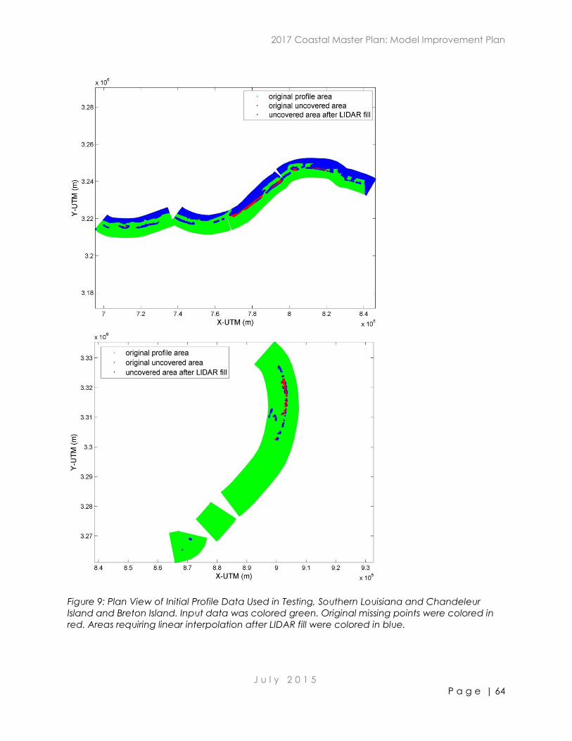
2017 Coastal Master Plan: Model Improvement Plan
J u l y 2 0 1 5
P a g e | 64
Figure 9: Plan View of Initial Profile Data Used in Testing, Southern Louisiana and Chandeleur
Island and Breton Island. Input data was colored green. Original missing points were colored in
red. Areas requiring linear interpolation after LIDAR fill were colored in blue.
2017 Coastal Master Plan: Model Improvement Plan
J u l y 2 0 1 5
P a g e | 65
14.3.2 Wave Transformation
Hindcast data from six WIS stations was used as input to drive the wave transformation using
SWAN. The locations of the WIS stations are shown in Figure 4 WIS stations 73124 and 73126, 73129
and 73131 were selected as the wave condition source for Isles Dernieres, Timbalier, Caminada
Headland and Grand Isle, Barataria Bay, respectively. WIS stations 73141 and 73139 were
selected for Chandeleur and Breton Islands. The wave data time series extends from January 1,
1980 to December 31, 2012, a period of 33 years with hourly record intervals. Figure 10 through
Figure 15 include the hourly wave data distribution for the 33-year record at the six WIS stations.
The distinct values selected to classify the wave bands are listed in Table 4.
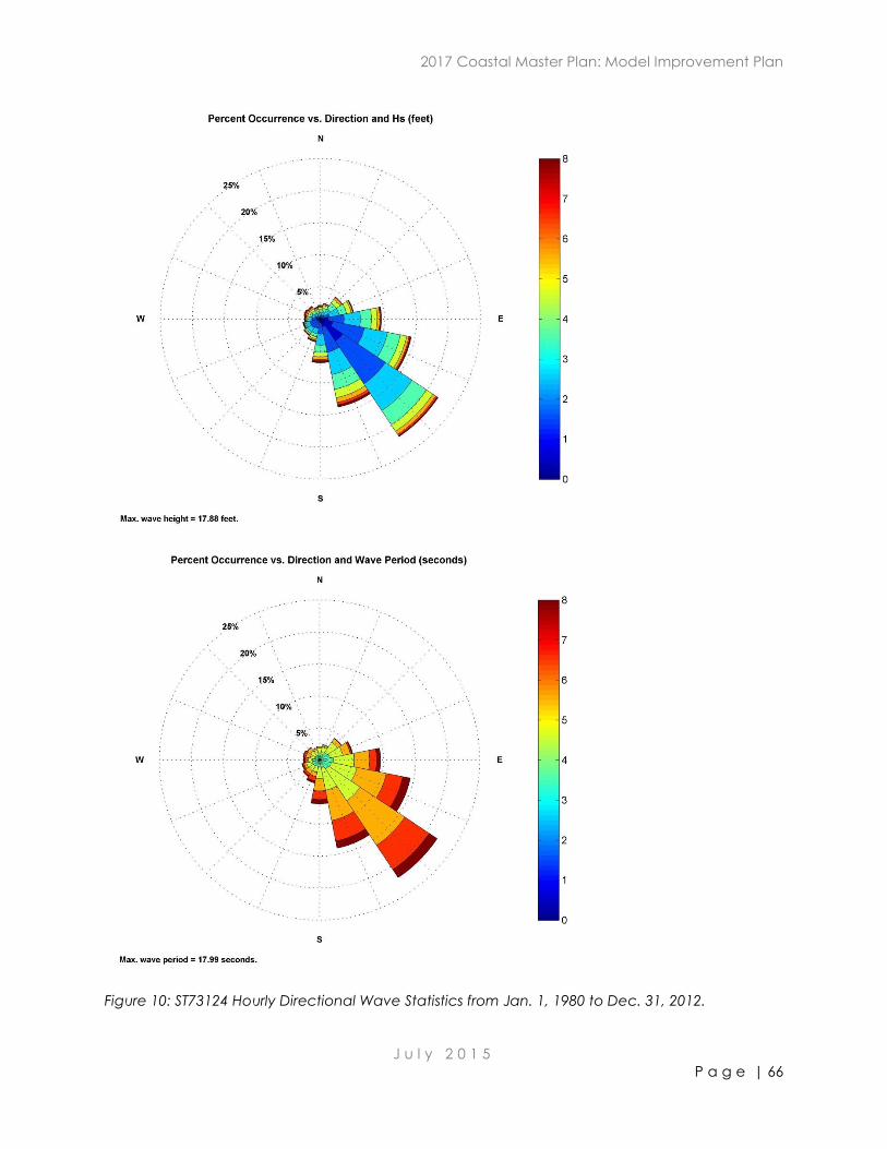
2017 Coastal Master Plan: Model Improvement Plan
J u l y 2 0 1 5
P a g e | 66
Figure 10: ST73124 Hourly Directional Wave Statistics from Jan. 1, 1980 to Dec. 31, 2012.
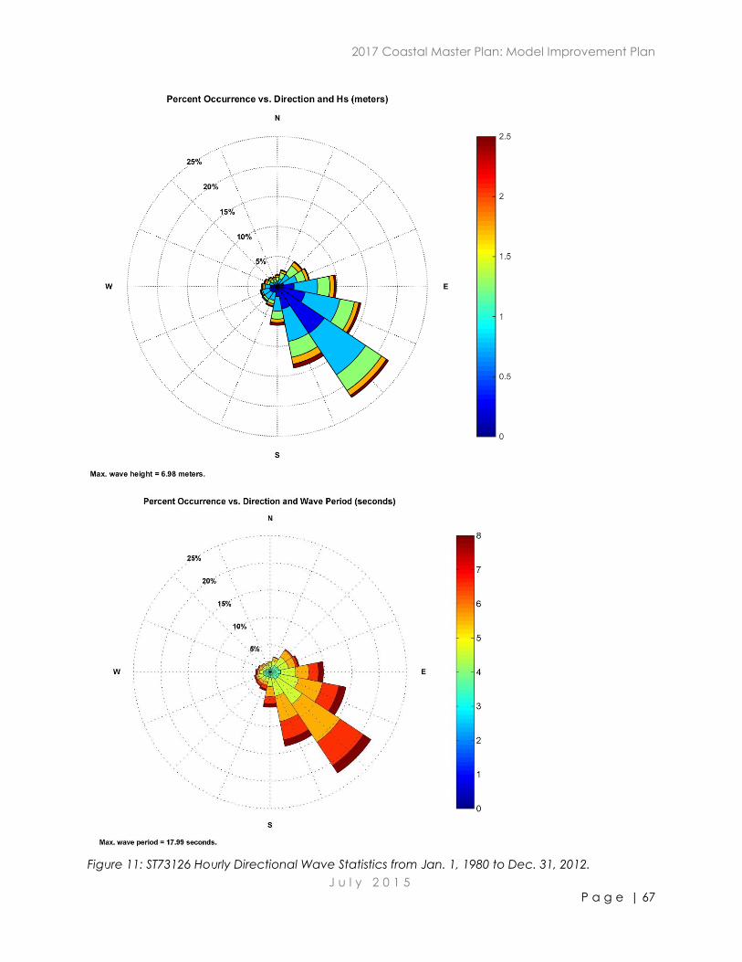
2017 Coastal Master Plan: Model Improvement Plan
J u l y 2 0 1 5
P a g e | 67
Figure 11: ST73126 Hourly Directional Wave Statistics from Jan. 1, 1980 to Dec. 31, 2012.
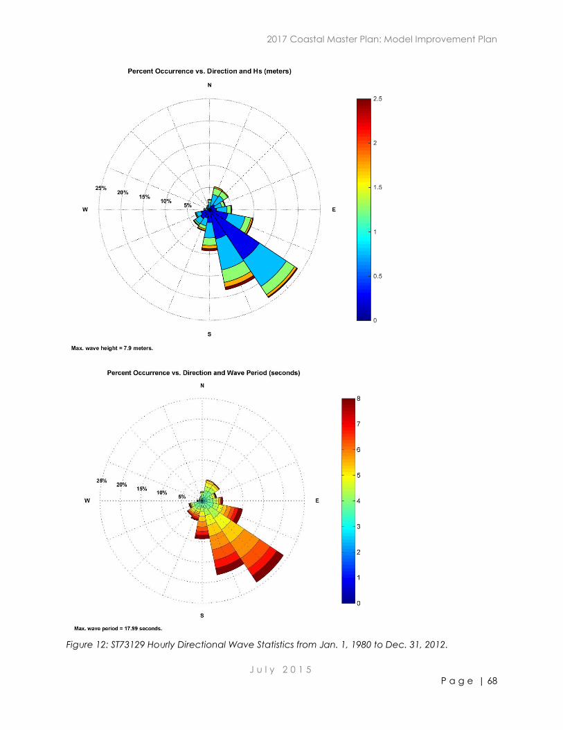
2017 Coastal Master Plan: Model Improvement Plan
J u l y 2 0 1 5
P a g e | 68
Figure 12: ST73129 Hourly Directional Wave Statistics from Jan. 1, 1980 to Dec. 31, 2012.
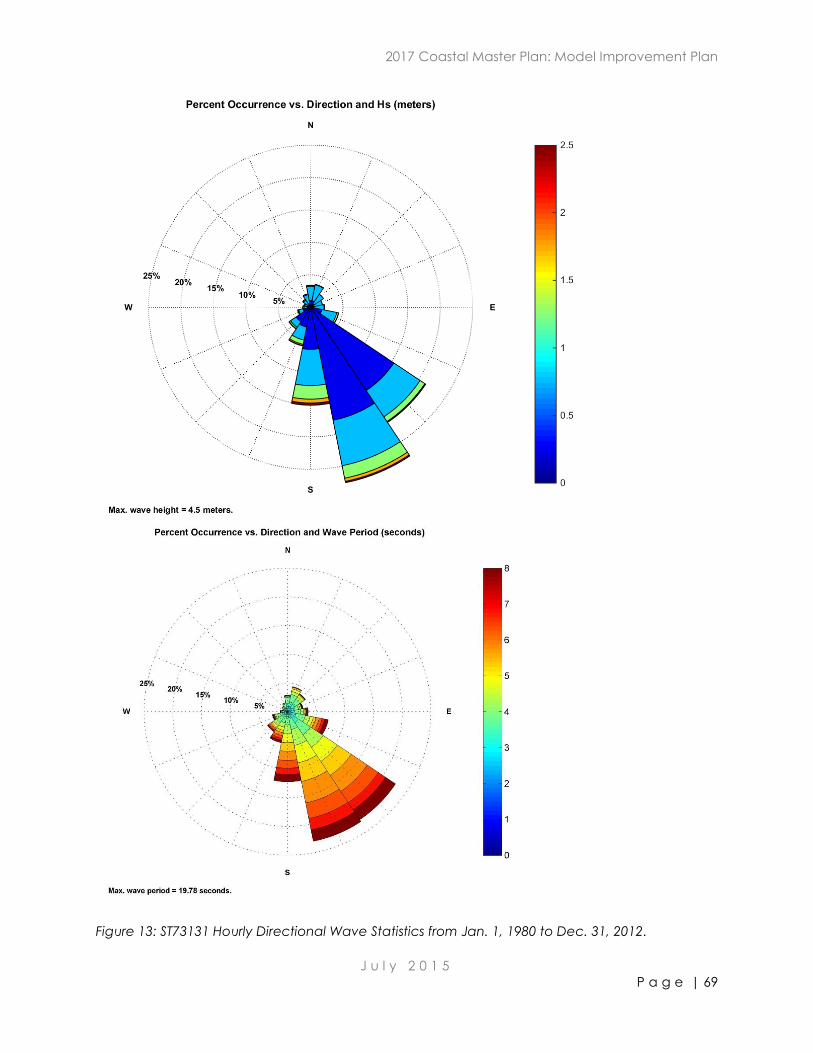
2017 Coastal Master Plan: Model Improvement Plan
J u l y 2 0 1 5
P a g e | 69
Figure 13: ST73131 Hourly Directional Wave Statistics from Jan. 1, 1980 to Dec. 31, 2012.
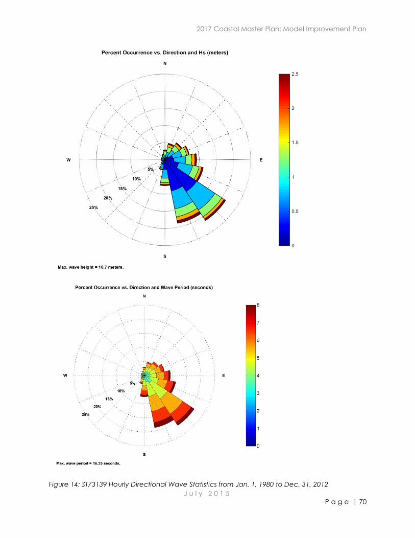
2017 Coastal Master Plan: Model Improvement Plan
J u l y 2 0 1 5
P a g e | 70
Figure 14: ST73139 Hourly Directional Wave Statistics from Jan. 1, 1980 to Dec. 31, 2012
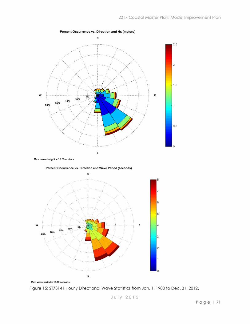
2017 Coastal Master Plan: Model Improvement Plan
J u l y 2 0 1 5
P a g e | 71
Figure 15: ST73141 Hourly Directional Wave Statistics from Jan. 1, 1980 to Dec. 31, 2012.
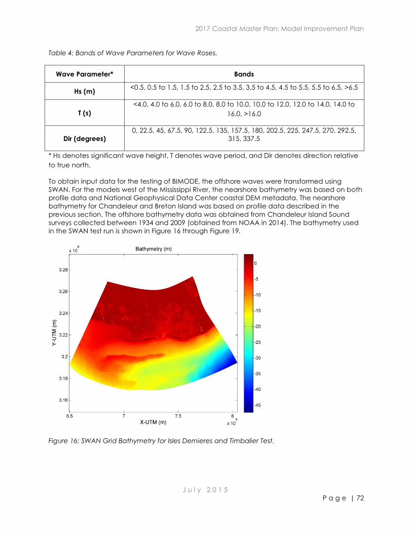
2017 Coastal Master Plan: Model Improvement Plan
J u l y 2 0 1 5
P a g e | 72
Table 4: Bands of Wave Parameters for Wave Roses.
Wave Parameter* Bands
Hs (m) <0.5, 0.5 to 1.5, 1.5 to 2.5, 2.5 to 3.5, 3.5 to 4.5, 4.5 to 5.5, 5.5 to 6.5, >6.5
T (s)
<4.0, 4.0 to 6.0, 6.0 to 8.0, 8.0 to 10.0, 10.0 to 12.0, 12.0 to 14.0, 14.0 to
16.0, >16.0
Dir (degrees)
0, 22.5, 45, 67.5, 90, 122.5, 135, 157.5, 180, 202.5, 225, 247.5, 270, 292.5,
315, 337.5
* Hs denotes significant wave height, T denotes wave period, and Dir denotes direction relative
to true north.
To obtain input data for the testing of BIMODE, the offshore waves were transformed using
SWAN. For the models west of the Mississippi River, the nearshore bathymetry was based on both
profile data and National Geophysical Data Center coastal DEM metadata. The nearshore
bathymetry for Chandeleur and Breton Island was based on profile data described in the
previous section. The offshore bathymetry data was obtained from Chandeleur Island Sound
surveys collected between 1934 and 2009 (obtained from NOAA in 2014). The bathymetry used
in the SWAN test run is shown in Figure 16 through Figure 19.
Figure 16: SWAN Grid Bathymetry for Isles Dernieres and Timbalier Test.
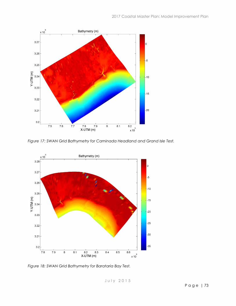
2017 Coastal Master Plan: Model Improvement Plan
J u l y 2 0 1 5
P a g e | 73
Figure 17: SWAN Grid Bathymetry for Caminada Headland and Grand Isle Test.
Figure 18: SWAN Grid Bathymetry for Barataria Bay Test.
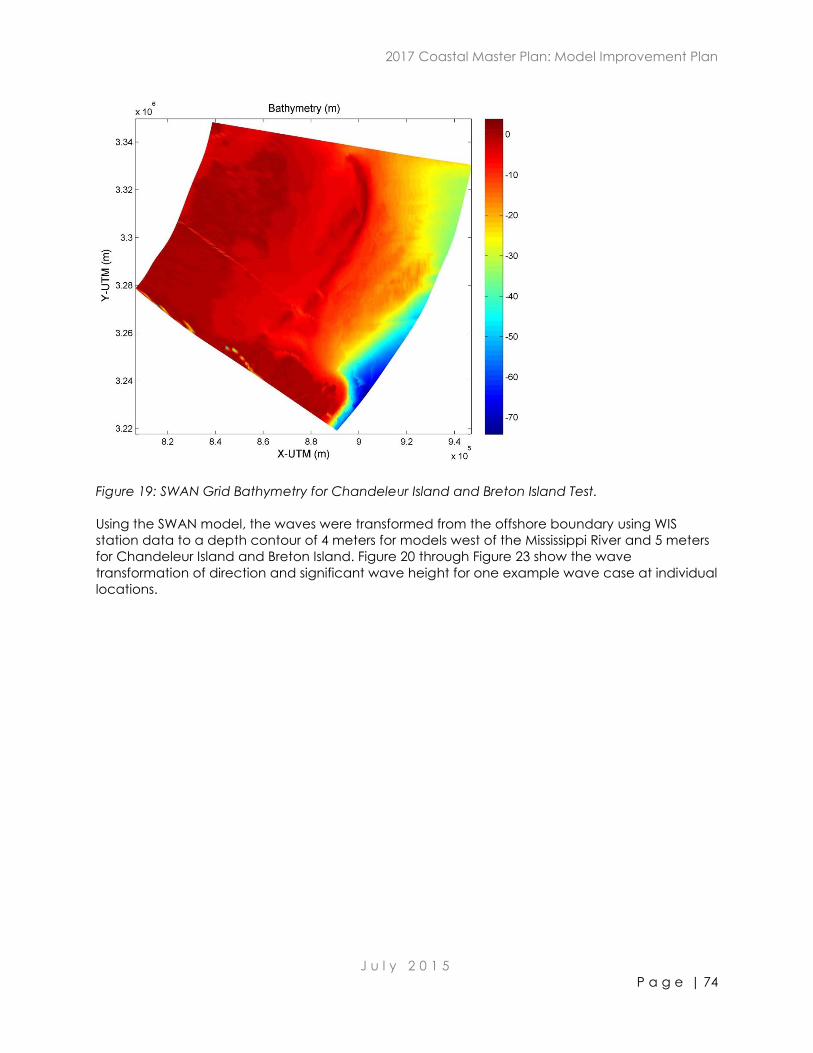
2017 Coastal Master Plan: Model Improvement Plan
J u l y 2 0 1 5
P a g e | 74
Figure 19: SWAN Grid Bathymetry for Chandeleur Island and Breton Island Test.
Using the SWAN model, the waves were transformed from the offshore boundary using WIS
station data to a depth contour of 4 meters for models west of the Mississippi River and 5 meters
for Chandeleur Island and Breton Island. Figure 20 through Figure 23 show the wave
transformation of direction and significant wave height for one example wave case at individual
locations.
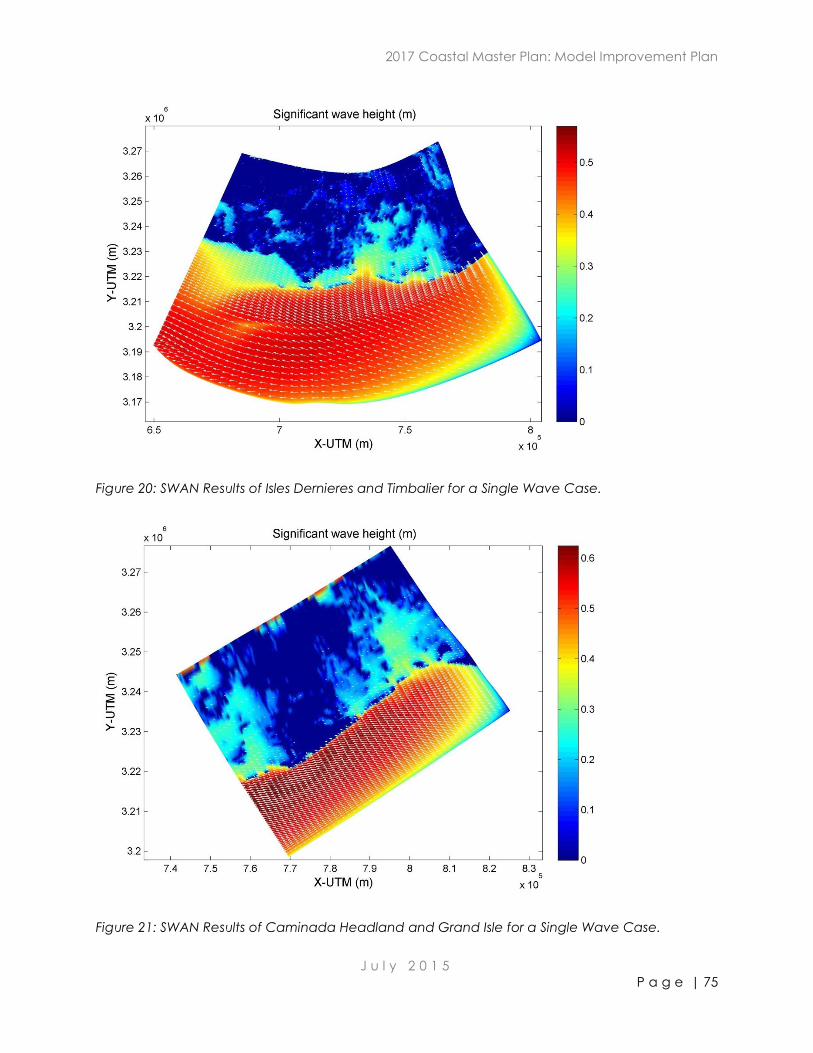
2017 Coastal Master Plan: Model Improvement Plan
J u l y 2 0 1 5
P a g e | 75
Figure 20: SWAN Results of Isles Dernieres and Timbalier for a Single Wave Case.
Figure 21: SWAN Results of Caminada Headland and Grand Isle for a Single Wave Case.
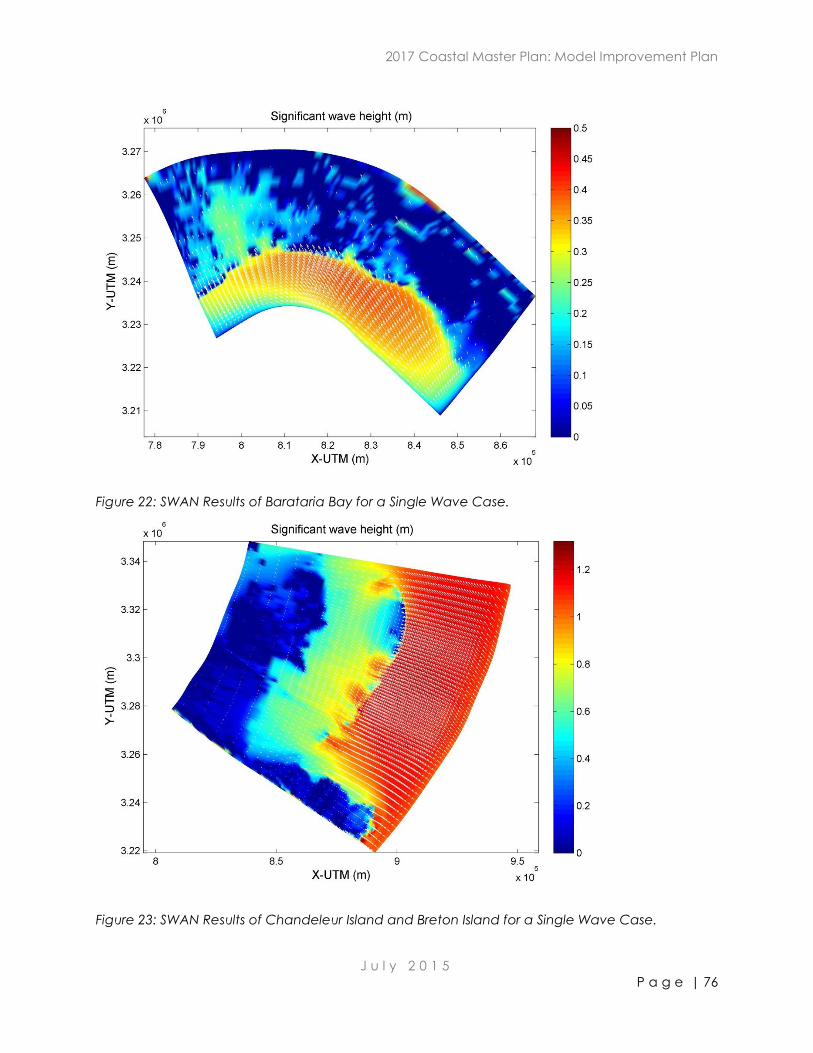
2017 Coastal Master Plan: Model Improvement Plan
J u l y 2 0 1 5
P a g e | 76
Figure 22: SWAN Results of Barataria Bay for a Single Wave Case.
Figure 23: SWAN Results of Chandeleur Island and Breton Island for a Single Wave Case.
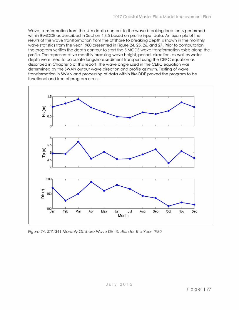
2017 Coastal Master Plan: Model Improvement Plan
J u l y 2 0 1 5
P a g e | 77
Wave transformation from the -4m depth contour to the wave breaking location is performed
within BIMODE as described in Section 4.3.5 based on profile input data. An example of the
results of this wave transformation from the offshore to breaking depth is shown in the monthly
wave statistics from the year 1980 presented in Figure 24, 25, 26, and 27. Prior to computation,
the program verifies the depth contour to start the BIMODE wave transformation exists along the
profile. The representative monthly breaking wave height, period, direction, as well as water
depth were used to calculate longshore sediment transport using the CERC equation as
described in Chapter 5 of this report. The wave angle used in the CERC equation was
determined by the SWAN output wave direction and profile azimuth. Testing of wave
transformation in SWAN and processing of data within BIMODE proved the program to be
functional and free of program errors.
Figure 24: ST71341 Monthly Offshore Wave Distribution for the Year 1980.
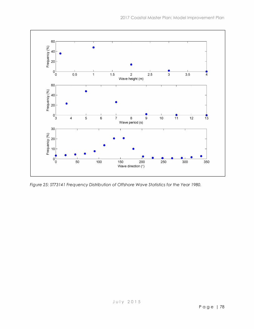
2017 Coastal Master Plan: Model Improvement Plan
J u l y 2 0 1 5
P a g e | 78
Figure 25: ST73141 Frequency Distribution of Offshore Wave Statistics for the Year 1980.
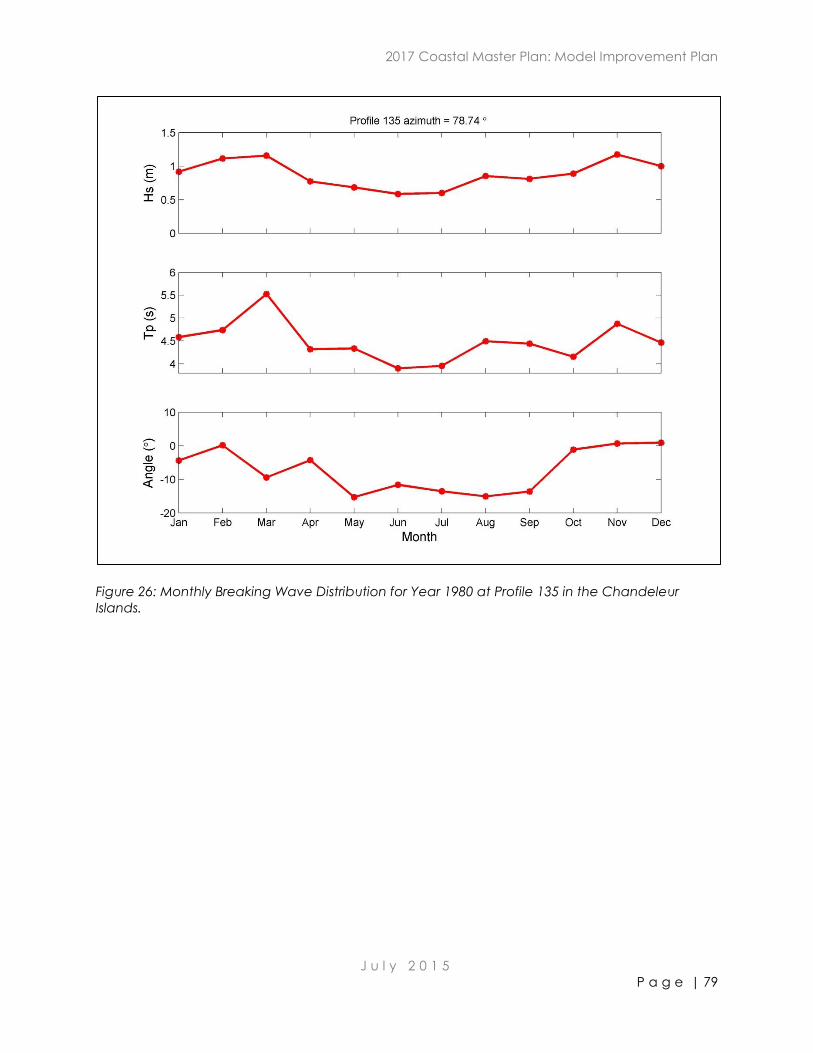
2017 Coastal Master Plan: Model Improvement Plan
J u l y 2 0 1 5
P a g e | 79
Figure 26: Monthly Breaking Wave Distribution for Year 1980 at Profile 135 in the Chandeleur
Islands.
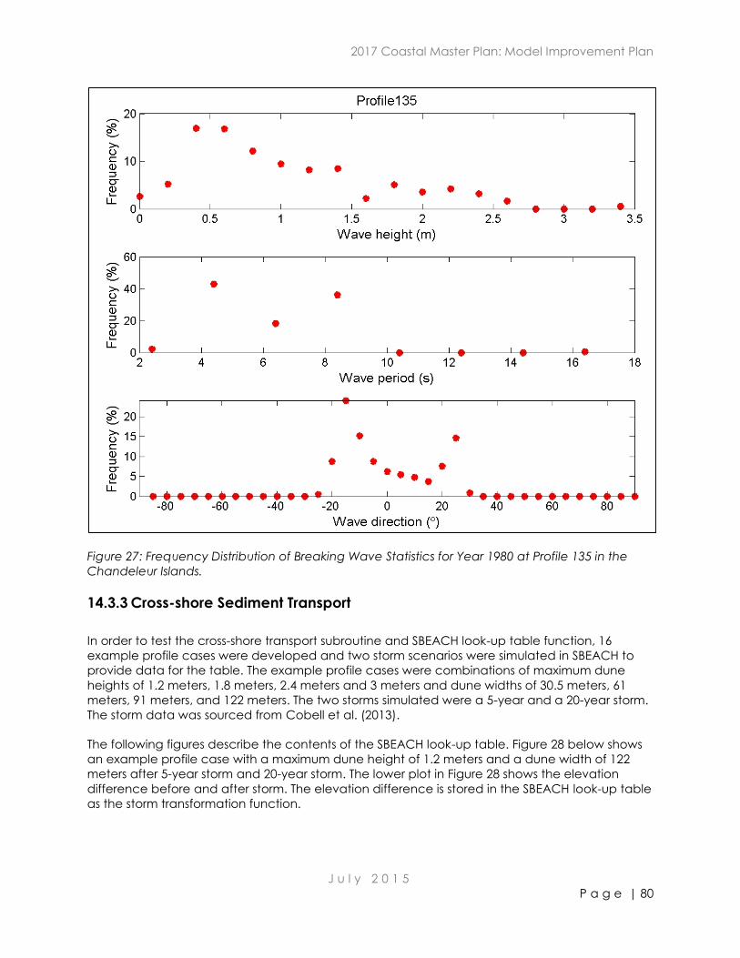
2017 Coastal Master Plan: Model Improvement Plan
J u l y 2 0 1 5
P a g e | 80
Figure 27: Frequency Distribution of Breaking Wave Statistics for Year 1980 at Profile 135 in the
Chandeleur Islands.
14.3.3 Cross-shore Sediment Transport
In order to test the cross-shore transport subroutine and SBEACH look-up table function, 16
example profile cases were developed and two storm scenarios were simulated in SBEACH to
provide data for the table. The example profile cases were combinations of maximum dune
heights of 1.2 meters, 1.8 meters, 2.4 meters and 3 meters and dune widths of 30.5 meters, 61
meters, 91 meters, and 122 meters. The two storms simulated were a 5-year and a 20-year storm.
The storm data was sourced from Cobell et al. (2013).
The following figures describe the contents of the SBEACH look-up table. Figure 28 below shows
an example profile case with a maximum dune height of 1.2 meters and a dune width of 122
meters after 5-year storm and 20-year storm. The lower plot in Figure 28 shows the elevation
difference before and after storm. The elevation difference is stored in the SBEACH look-up table
as the storm transformation function.
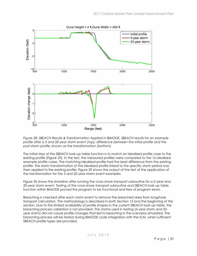
2017 Coastal Master Plan: Model Improvement Plan
J u l y 2 0 1 5
P a g e | 81
Figure 28: SBEACH Results & Transformation Applied in BIMODE. SBEACH results for an example
profile after a 5 and 20-year storm event (top); difference between the initial profile and the
post-storm profile, known as the transformation (bottom).
The initial step of the SBEACH look-up table function is to match an idealized profile case to the
existing profile (Figure 29). In the test, the measured profiles were compared to the 16 idealized
example profile cases. The matching idealized profile had the least difference from the existing
profile. The storm transformation of the idealized profile linked to the specific storm period was
then applied to the existing profile. Figure 29 shows the output of the test of the application of
the transformation for the 5 and 20-year storm event examples.
Figure 30 shows the shoreline after running the cross-shore transport subroutine for a 5-year and
20-year storm event. Testing of the cross-shore transport subroutine and SBEACH look-up table
function within BIMODE proved the program to be functional and free of program errors.
Breaching is checked after each storm event to remove the breached area from longshore
transport calculation. The methodology is described in both Section 13 and the beginning of this
section. Due to the limited availability of profile shapes in the current SBEACH look-up table, the
breaching process validation is not provided. The storms used in testing (5-year storm and 20-
year storm) did not cause profile changes that led to beaching in the scenarios simulated. The
breaching process will be tested during BIMODE code integration with the ICM, when sufficient
SBEACH profile types are provided.
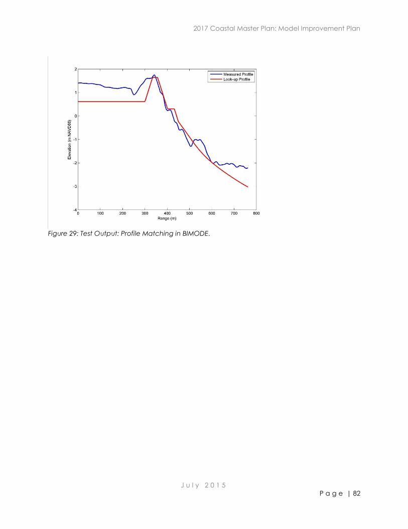
2017 Coastal Master Plan: Model Improvement Plan
J u l y 2 0 1 5
P a g e | 82
Figure 29: Test Output: Profile Matching in BIMODE.
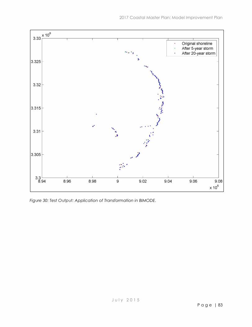
2017 Coastal Master Plan: Model Improvement Plan
J u l y 2 0 1 5
P a g e | 83
Figure 30: Test Output: Application of Transformation in BIMODE.
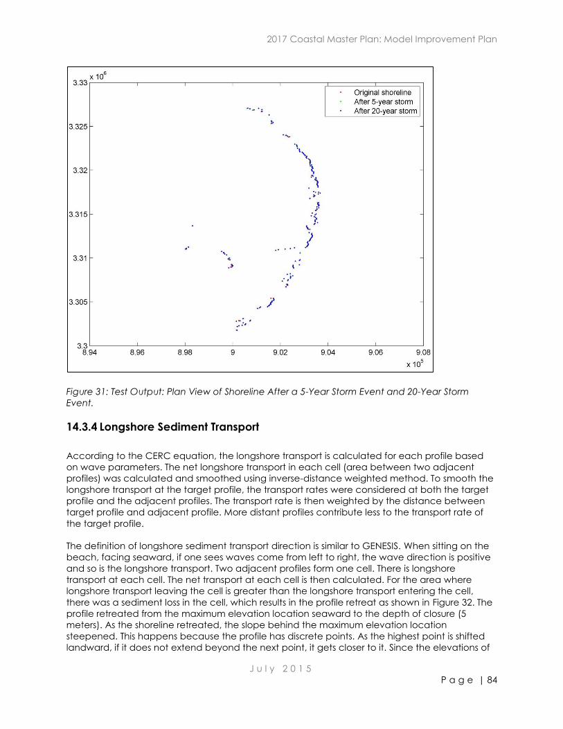
2017 Coastal Master Plan: Model Improvement Plan
J u l y 2 0 1 5
P a g e | 84
Figure 31: Test Output: Plan View of Shoreline After a 5-Year Storm Event and 20-Year Storm
Event.
14.3.4 Longshore Sediment Transport
According to the CERC equation, the longshore transport is calculated for each profile based
on wave parameters. The net longshore transport in each cell (area between two adjacent
profiles) was calculated and smoothed using inverse-distance weighted method. To smooth the
longshore transport at the target profile, the transport rates were considered at both the target
profile and the adjacent profiles. The transport rate is then weighted by the distance between
target profile and adjacent profile. More distant profiles contribute less to the transport rate of
the target profile.
The definition of longshore sediment transport direction is similar to GENESIS. When sitting on the
beach, facing seaward, if one sees waves come from left to right, the wave direction is positive
and so is the longshore transport. Two adjacent profiles form one cell. There is longshore
transport at each cell. The net transport at each cell is then calculated. For the area where
longshore transport leaving the cell is greater than the longshore transport entering the cell,
there was a sediment loss in the cell, which results in the profile retreat as shown in Figure 32. The
profile retreated from the maximum elevation location seaward to the depth of closure (5
meters). As the shoreline retreated, the slope behind the maximum elevation location
steepened. This happens because the profile has discrete points. As the highest point is shifted
landward, if it does not extend beyond the next point, it gets closer to it. Since the elevations of
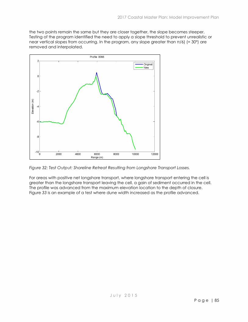
2017 Coastal Master Plan: Model Improvement Plan
J u l y 2 0 1 5
P a g e | 85
the two points remain the same but they are closer together, the slope becomes steeper.
Testing of the program identified the need to apply a slope threshold to prevent unrealistic or
near vertical slopes from occurring. In the program, any slope greater than π/6) (= 30º) are
removed and interpolated.
Figure 32: Test Output: Shoreline Retreat Resulting from Longshore Transport Losses.
For areas with positive net longshore transport, where longshore transport entering the cell is
greater than the longshore transport leaving the cell, a gain of sediment occurred in the cell.
The profile was advanced from the maximum elevation location to the depth of closure.
Figure 33 is an example of a test where dune width increased as the profile advanced.
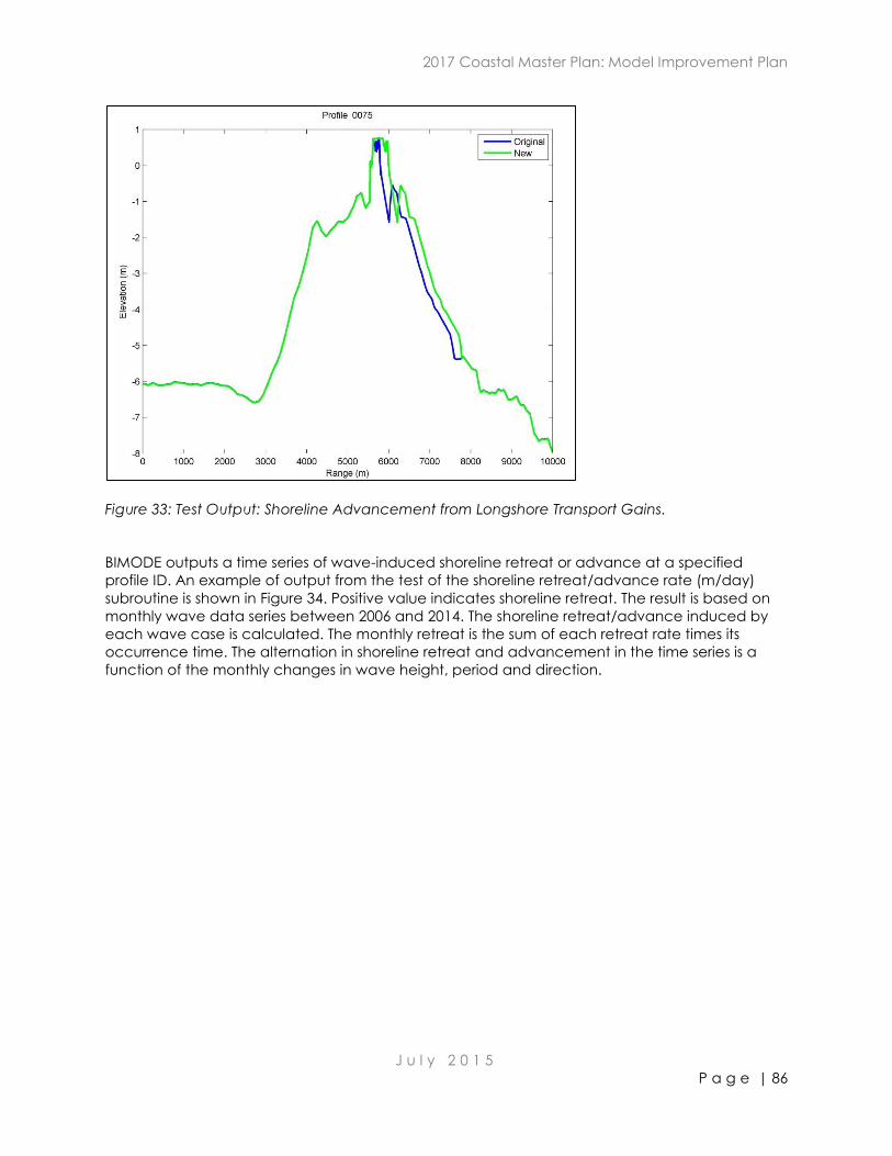
2017 Coastal Master Plan: Model Improvement Plan
J u l y 2 0 1 5
P a g e | 86
Figure 33: Test Output: Shoreline Advancement from Longshore Transport Gains.
BIMODE outputs a time series of wave-induced shoreline retreat or advance at a specified
profile ID. An example of output from the test of the shoreline retreat/advance rate (m/day)
subroutine is shown in Figure 34. Positive value indicates shoreline retreat. The result is based on
monthly wave data series between 2006 and 2014. The shoreline retreat/advance induced by
each wave case is calculated. The monthly retreat is the sum of each retreat rate times its
occurrence time. The alternation in shoreline retreat and advancement in the time series is a
function of the monthly changes in wave height, period and direction.
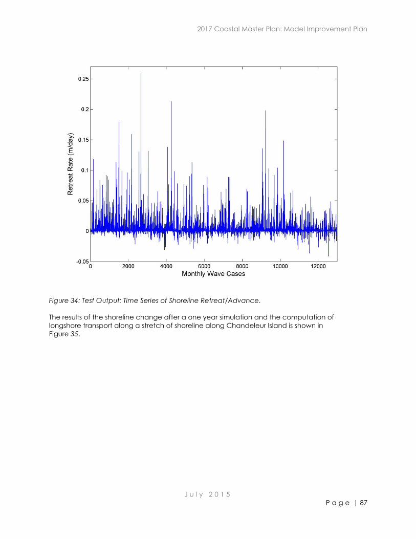
2017 Coastal Master Plan: Model Improvement Plan
J u l y 2 0 1 5
P a g e | 87
Figure 34: Test Output: Time Series of Shoreline Retreat/Advance.
The results of the shoreline change after a one year simulation and the computation of
longshore transport along a stretch of shoreline along Chandeleur Island is shown in
Figure 35.
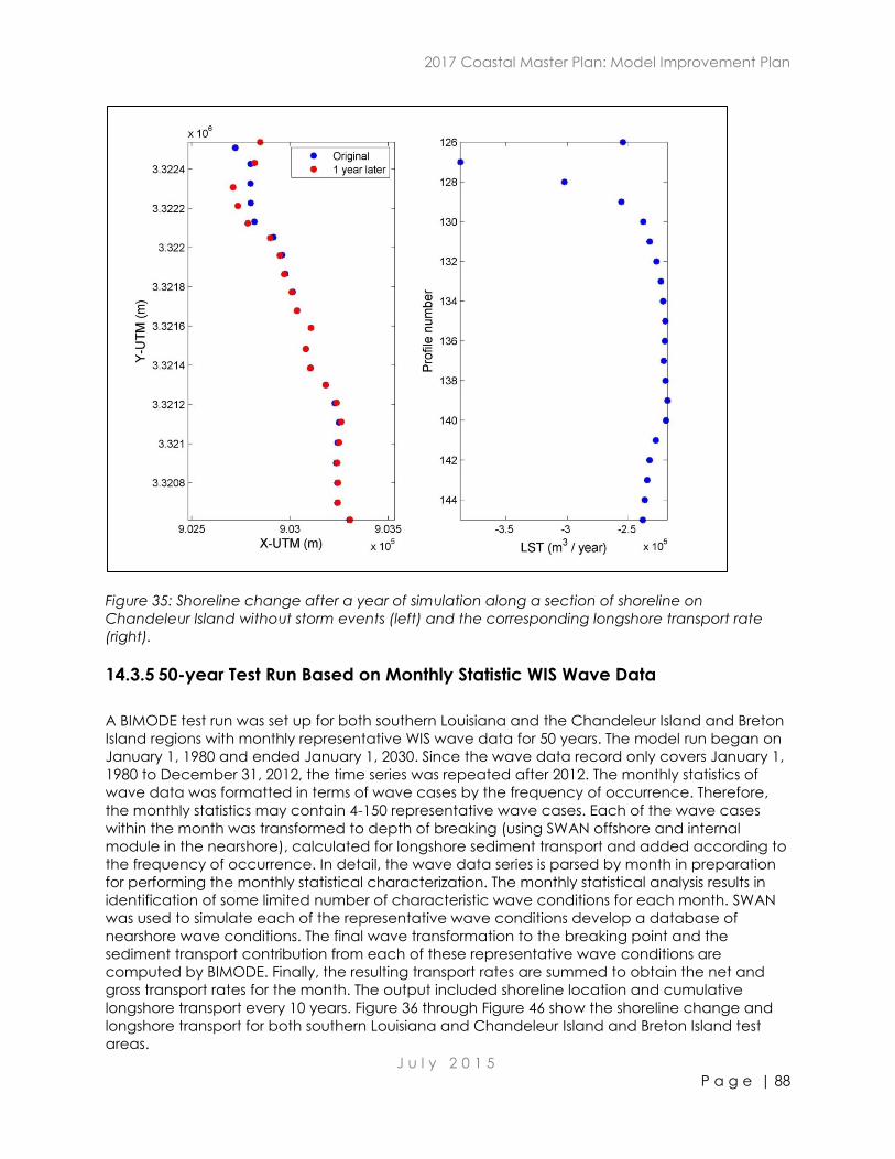
2017 Coastal Master Plan: Model Improvement Plan
J u l y 2 0 1 5
P a g e | 88
Figure 35: Shoreline change after a year of simulation along a section of shoreline on
Chandeleur Island without storm events (left) and the corresponding longshore transport rate
(right).
14.3.5 50-year Test Run Based on Monthly Statistic WIS Wave Data
A BIMODE test run was set up for both southern Louisiana and the Chandeleur Island and Breton
Island regions with monthly representative WIS wave data for 50 years. The model run began on
January 1, 1980 and ended January 1, 2030. Since the wave data record only covers January 1,
1980 to December 31, 2012, the time series was repeated after 2012. The monthly statistics of
wave data was formatted in terms of wave cases by the frequency of occurrence. Therefore,
the monthly statistics may contain 4-150 representative wave cases. Each of the wave cases
within the month was transformed to depth of breaking (using SWAN offshore and internal
module in the nearshore), calculated for longshore sediment transport and added according to
the frequency of occurrence. In detail, the wave data series is parsed by month in preparation
for performing the monthly statistical characterization. The monthly statistical analysis results in
identification of some limited number of characteristic wave conditions for each month. SWAN
was used to simulate each of the representative wave conditions develop a database of
nearshore wave conditions. The final wave transformation to the breaking point and the
sediment transport contribution from each of these representative wave conditions are
computed by BIMODE. Finally, the resulting transport rates are summed to obtain the net and
gross transport rates for the month. The output included shoreline location and cumulative
longshore transport every 10 years. Figure 36 through Figure 46 show the shoreline change and
longshore transport for both southern Louisiana and Chandeleur Island and Breton Island test
areas.
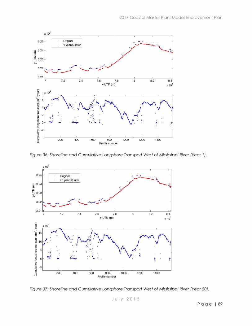
2017 Coastal Master Plan: Model Improvement Plan
J u l y 2 0 1 5
P a g e | 89
Figure 36: Shoreline and Cumulative Longshore Transport West of Mississippi River (Year 1).
Figure 37: Shoreline and Cumulative Longshore Transport West of Mississippi River (Year 20).
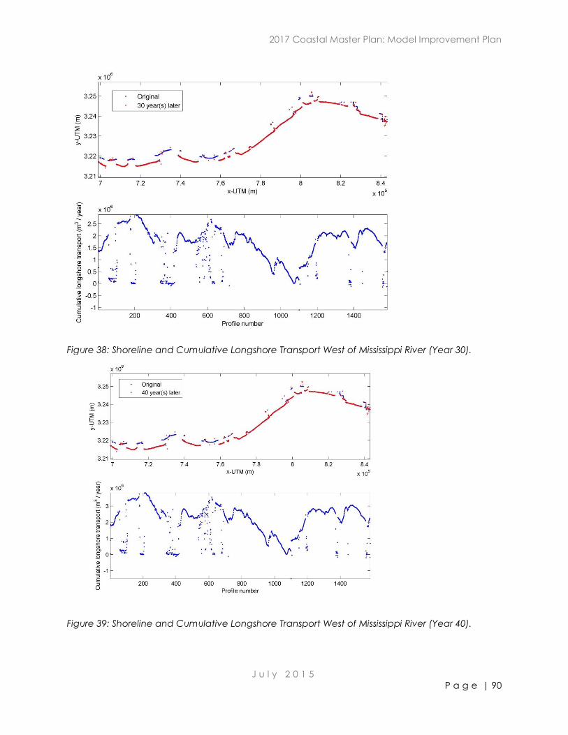
2017 Coastal Master Plan: Model Improvement Plan
J u l y 2 0 1 5
P a g e | 90
Figure 38: Shoreline and Cumulative Longshore Transport West of Mississippi River (Year 30).
Figure 39: Shoreline and Cumulative Longshore Transport West of Mississippi River (Year 40).
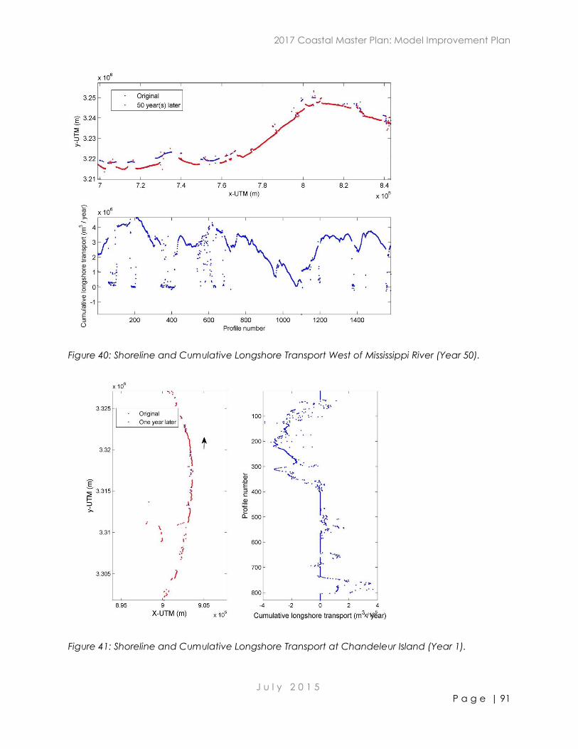
2017 Coastal Master Plan: Model Improvement Plan
J u l y 2 0 1 5
P a g e | 91
Figure 40: Shoreline and Cumulative Longshore Transport West of Mississippi River (Year 50).
Figure 41: Shoreline and Cumulative Longshore Transport at Chandeleur Island (Year 1).
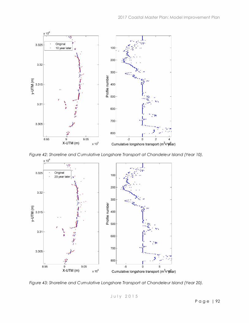
2017 Coastal Master Plan: Model Improvement Plan
J u l y 2 0 1 5
P a g e | 92
Figure 42: Shoreline and Cumulative Longshore Transport at Chandeleur Island (Year 10).
Figure 43: Shoreline and Cumulative Longshore Transport at Chandeleur Island (Year 20).
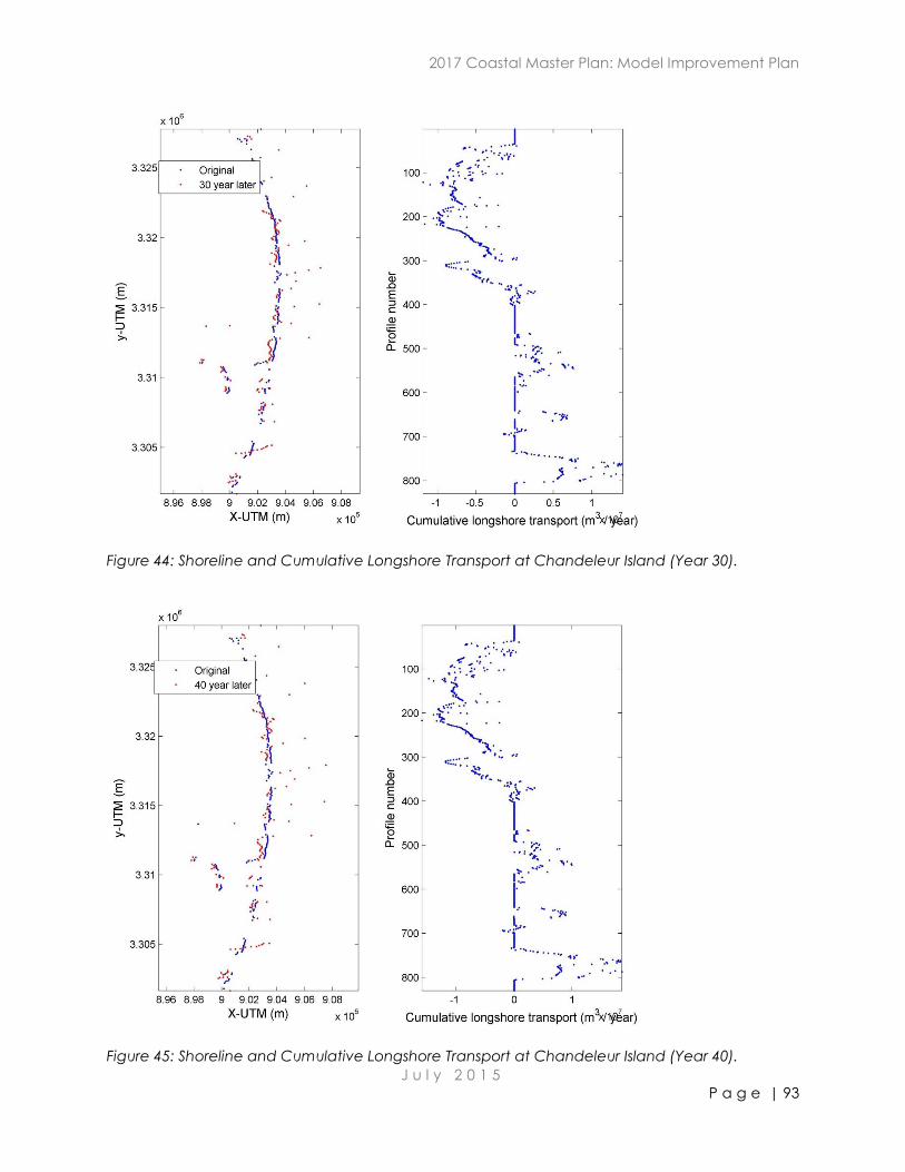
2017 Coastal Master Plan: Model Improvement Plan
J u l y 2 0 1 5
P a g e | 93
Figure 44: Shoreline and Cumulative Longshore Transport at Chandeleur Island (Year 30).
Figure 45: Shoreline and Cumulative Longshore Transport at Chandeleur Island (Year 40).
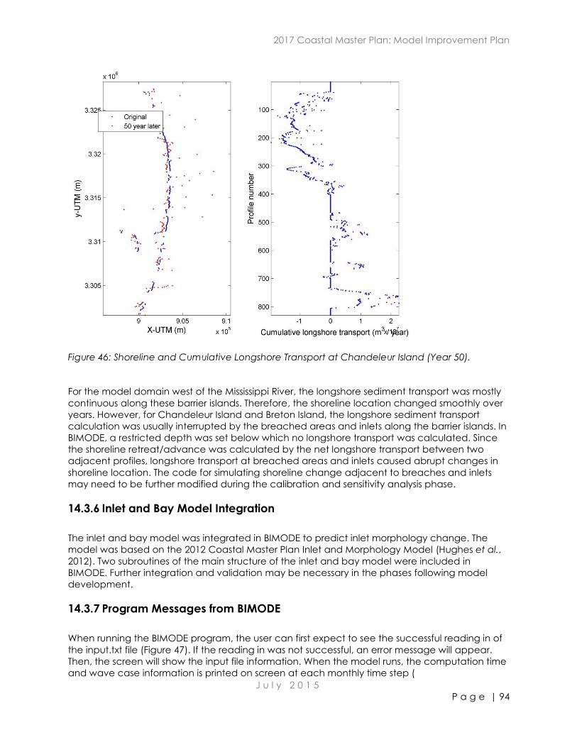
2017 Coastal Master Plan: Model Improvement Plan
J u l y 2 0 1 5
P a g e | 94
Figure 46: Shoreline and Cumulative Longshore Transport at Chandeleur Island (Year 50).
For the model domain west of the Mississippi River, the longshore sediment transport was mostly
continuous along these barrier islands. Therefore, the shoreline location changed smoothly over
years. However, for Chandeleur Island and Breton Island, the longshore sediment transport
calculation was usually interrupted by the breached areas and inlets along the barrier islands. In
BIMODE, a restricted depth was set below which no longshore transport was calculated. Since
the shoreline retreat/advance was calculated by the net longshore transport between two
adjacent profiles, longshore transport at breached areas and inlets caused abrupt changes in
shoreline location. The code for simulating shoreline change adjacent to breaches and inlets
may need to be further modified during the calibration and sensitivity analysis phase.
14.3.6 Inlet and Bay Model Integration
The inlet and bay model was integrated in BIMODE to predict inlet morphology change. The
model was based on the 2012 Coastal Master Plan Inlet and Morphology Model (Hughes et al.,
2012). Two subroutines of the main structure of the inlet and bay model were included in
BIMODE. Further integration and validation may be necessary in the phases following model
development.
14.3.7 Program Messages from BIMODE
When running the BIMODE program, the user can first expect to see the successful reading in of
the input.txt file (Figure 47). If the reading in was not successful, an error message will appear.
Then, the screen will show the input file information. When the model runs, the computation time
and wave case information is printed on screen at each monthly time step (
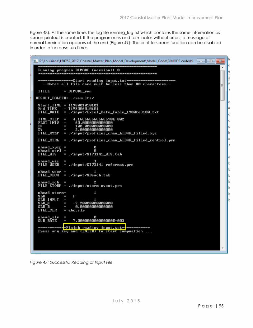
2017 Coastal Master Plan: Model Improvement Plan
J u l y 2 0 1 5
P a g e | 95
Figure 48). At the same time, the log file running_log.txt which contains the same information as
screen printout is created. If the program runs and terminates without errors, a message of
normal termination appears at the end (Figure 49). The print to screen function can be disabled
in order to increase run times.
Figure 47: Successful Reading of Input File.
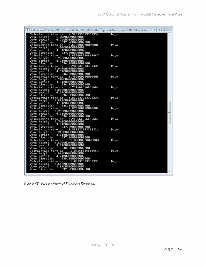
2017 Coastal Master Plan: Model Improvement Plan
J u l y 2 0 1 5
P a g e | 96
Figure 48: Screen View of Program Running.
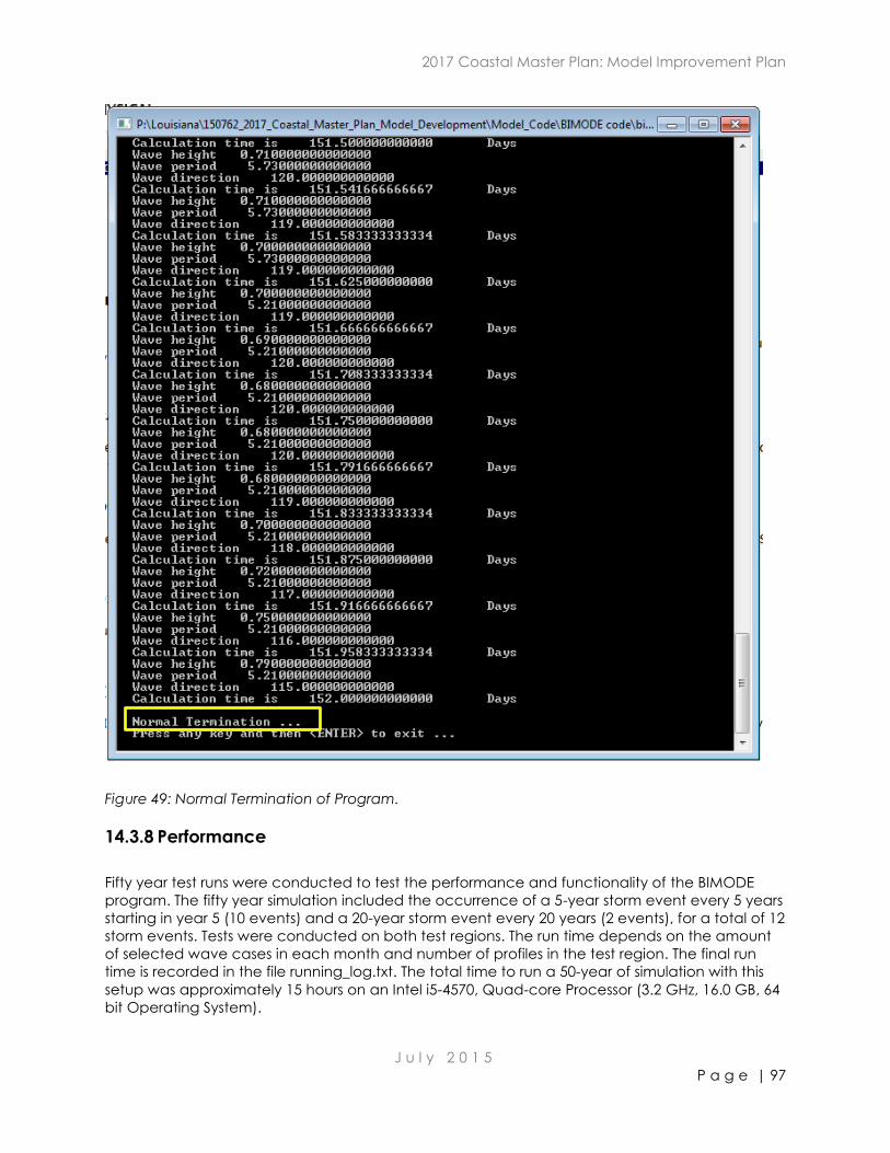
2017 Coastal Master Plan: Model Improvement Plan
J u l y 2 0 1 5
P a g e | 97
Figure 49: Normal Termination of Program.
14.3.8 Performance
Fifty year test runs were conducted to test the performance and functionality of the BIMODE
program. The fifty year simulation included the occurrence of a 5-year storm event every 5 years
starting in year 5 (10 events) and a 20-year storm event every 20 years (2 events), for a total of 12
storm events. Tests were conducted on both test regions. The run time depends on the amount
of selected wave cases in each month and number of profiles in the test region. The final run
time is recorded in the file running_log.txt. The total time to run a 50-year of simulation with this
setup was approximately 15 hours on an Intel i5-4570, Quad-core Processor (3.2 GHz, 16.0 GB, 64
bit Operating System).
2017 Coastal Master Plan: Model Improvement Plan
J u l y 2 0 1 5
P a g e | 98
15.0 Conclusions
A critical component of 2017 Coastal Master Plan is predicting the evolution of Louisiana’s
barrier islands. The 2017 Model Improvement Plan (CPRA, 2013) builds upon the modeling
developed for the 2012 Coastal Master Plan (CPRA, 2012). Models must be capable of
simulating 50-year time periods in an efficient manner and predicting project effects at a basin-
scale. Specifically, the BIMODE improvements include modeling additional physical processes
(e.g., overwash), improving the capabilities of predicting change in island morphology, and
incorporating realistic event-driven morphodynamic responses. Another key advantage of
BIMODE is the ability to be integrated into the ICM. The scope of this effort included a literature
review; model approach development; and model formulation, coding, and testing; along with
working meetings, routine teleconferences, and reporting. The focus area includes from the
Chandeleur Islands to the eastern side of the Mississippi River active Balize Delta and from
Scofield Island to Raccoon Island on the western side of the Mississippi River active Balize Delta.
Based upon a detailed review of pertinent available literature, knowledge and experience from
restoration project design and field data collection, and professional judgment, the BIMODE
Team selected the following physical processes, forcing functions, and geomorphic forms that
affect the evolution of Louisiana’s barrier islands for consideration in developing the modeling
approach: wave transformation, longshore sediment transport, cross-shore sediment transport,
breaching, inlets and bays, post-storm recovery, subsidence, and ESLR. Aeolian processes are
not included in the BIMODE model, and the rationale for not incorporating this process is
provided herein.
A hybrid modeling approach was developed to account for the key physical processes of
longshore and cross-shore sediment transport. The longshore transport model formulation
includes a three step wave transformation process using available hindcast data to yield
representative breaking wave conditions. Wave data are used to estimate sediment transport
rates employing the CERC transport formulation. Calibration of the longshore transport rates will
be accomplished through comparisons to published data; note: calibration procedure and
outcomes will be documented separately. The cross-shore sediment transport formulation
includes application of the one-dimensional model SBEACH that simulates cross-shore
morphologic response to a storm event based on measurement derived, empirical equations.
The SBEACH model runs are recalled through look-up tables to determine the likely output profile
given the starting input profile and storm characteristics. Input profiles are based on
representative static submerged profiles from each of the regions along with combination of
varying dune heights, dune widths and berm widths, some of which will represent pre-restoration
barrier island profiles. The cross-shore transport formulation will be calibrated to demonstrate the
predictive capability of the model across the study area for the selected range of storms.
Based upon experience in restoration project design, SBEACH tends to under predict storm
erosion, which in some sense accounts for post-storm recovery processes. Accordingly, the
BIMODE Team suggests the post-storm recovery processes are captured sufficiently through
application of SBEACH.
Barrier island breaching is incorporated into the BIMODE model by determining critical thresholds
of minimum barrier island widths and minimum width to island length ratios through application
of historical data on barrier island breaching.
Subsidence and ESLR are incorporated into the BIMODE model through manual adjustments per
guidance provided by CPRA.

2017 Coastal Master Plan: Model Improvement Plan
J u l y 2 0 1 5
P a g e | 99
The barrier shoreline model employed in the 2012 modeling accounted for inlet and bay
processes, specifically inlet expansion/enlargement, using equilibrium theory for inlet cross-
sectional area as a function of tidal prism. The BIMODE model utilizes the 2012 model formulation
for inlets and bays, and can be coupled with the hydrology subroutine of the ICM more
frequently, e.g., yearly, than was possible in 2012.
The procedure for the BIMODE model includes reading in the profile and wave data inputs,
determining longshore sediment transport, locating nodal points where sediment transport
diverges, determining net erosion or accretion within each cell formed by two adjacent profiles,
and computing change in beach face profile specific to longshore transport; adjusting beach
profiles to account for relative sea level rise, beach face profile retreat due to silt loss, and
consolidation; accounting for cross-shore sediment transport for the given storm suite; eroding
bayward side of profile; checking for and implementing breaching if the thresholds are met; and
incorporating the inlet and bay model; and repeating for the 50-year simulation period. Output
is cross-sections at each emergent profile in the format of a DEM.
BIMODE.f90 is the executable program developed to simulate the physical processes outlined in
the procedures. BIMODE was written in Fortran 90. The file structure of the program consists of a
main program file, which calls on several process-based subroutines to run. Quality control
testing of the functionality and performance of the individual subroutines and code in its entirety
was performed. Fifty year test runs were set up for two regions, Southern Louisiana and the
Chandeleur Island and Breton Island complex, and included the occurrence of 12 return-interval
storm events. In the final tests, the program ran to completion successfully and without program
errors. Based on the input data used for testing and the results, additional model validation and
modification may be necessary to refine the processes included in the model and to integrate
BIMODE into the ICM. Validation of the breaching process is necessary since only a limited
number of profile shapes were included in the SBEACH look-up table used for testing. Further
integration and validation of the inlet and bay model is necessary in the following phases of
model development. In correlation, the code for simulating shoreline change adjacent to
breaches and inlets may need to be further modified based on the results of the calibration and
sensitivity phase.
2017 Coastal Master Plan: Model Improvement Plan
J u l y 2 0 1 5
P a g e | 100
16.0 References
Bagnold, R.A. (1941). The physics of wind-blown sand and desert dunes. Methuen, London, p.
265.
Bagnold, R.A. (1936). The movement of desert sand, Proceedings of the Royal Society of London.
Series A, Mathematical and Physical Sciences, 157( 892), 594-620.
Basco, D., & Shin, C. (1999). A One-Dimensional Numerical Model for Storm-Breaching of Barrier
Islands. Journal of Coastal Research, 15(1), 241-260. ISSN 0749-0208.
Bijker, E.W. (1971). Longshore transport computations. Proc. ASCE, Journal of the Waterways,
Harbors and Coastal Engineering Division, WW4.
Bijker, E.W. (1967). Some considerations about scales for coastal models with movable bed. Delft
Hydraulics Laboratory, Publication No. 50, Delft.
Bodge, K.R. (1989). A Literature Review of the Distribution of Longshore Sediment Transport across
the Surf Zone. Journal of Coastal Research, 5(2), 307-328.
Bonanata, R., Medina, R., Silveira, L., & Benedet, L. (2010). Methodology for the Characterization
of the Marine Climate at a Point Near the Coast from a series of Deep Water Data. VI
Argentine Congress of Port Engineering.
Booij, N., Holthuijsen, L.H., & Ris, R.C. (1996). The SWAN wave model for shallow water,
Proceedings of the 25th International Conference on Coastal Engineering. Orlando,
Florida. Vol. 1, pp. 668-676.
Bruun, P. (1962). Sea-Level Rise as a Cause of Erosion. Published Monthly of the Florida
Engineering and Industrial Experiment Station, Vol XVI, No. 5, pp. 2-15.
Bruun, P. (1954). Coast erosion and the development of beach profiles. Technical Memorandum,
vol. 44. Beach Erosion Board, U.S. Army Corps of Engineers, 82 pp.
Bruun, P., & Gerritsen, F. (1960). Stability of Tidal Inlets. North Holland, Amsterdam. 123 pp.
Campbell, T. (2005). Development of a Conceptual Morphosedimentary Model for Design of
Coastal Restoration Projects Along the Louisiana Coast. Journal of Coastal Research,
Special Issue 44, 234 -244.
Campbell, T., Benedet, L, & Thomson, G. (2005). Design Considerations for Barrier Island
Nourishments and Coastal Structures for Coastal Restoration in Louisiana. Journal of
Coastal Research. SI44, 186-202.
Coast & Harbor Engineering, Inc. with Hartman Engineering, Inc. (2007). Grand Isle Barrier
Shoreline Stabilization Study, Preliminary Engineering Report, Part 1: Basis for Engineering.
Prepared for State of Louisiana Department of Natural Resources.
Coastal Engineering Consultants, Inc. (2013). Barrier System Performance Assessment, Technical
Memorandum 4, Louisiana Barrier Island Restoration Performance Analysis. Prepared for
the Coastal Protection and Restoration Authority of Louisiana.
2017 Coastal Master Plan: Model Improvement Plan
J u l y 2 0 1 5
P a g e | 101
Coastal Engineering Consultants, Inc. (2011). Caminada Headland Beach and Dune Restoration
(BA-45), Headland Restoration Template Alternatives Analysis Report. Prepared for the
Coastal Protection and Restoration Authority of Louisiana.
Coastal Engineering Consultants, Inc. and SJB Group, Inc. (2008). Barataria Barrier Shoreline
Restoration Feasibility - Study Appendix C, Caminada Headland, Lafourche Parish,
Louisiana. Prepared for State of Louisiana Department of Natural Resources, Office of
Coastal Restoration Management, Coastal Engineering Division.
Coastal Engineering Research Center (1984). Shore Protection Manual (p.607). Washington,
D.C.: US Army Corps of Engineers, US Government Printing Office.
Coastal Planning & Engineering, Inc. (2005). East and West Grand Terre Island Restoration Project
(BA-30) - 30% Design Review Report. Boca Raton, Florida: Coastal Planning & Engineering,
Inc.
Coastal Planning & Engineering, Inc. (2004). Raccoon Island Project (TE-48) Sediment Budget,
Terrebonne Parish, Louisiana. Boca Raton, Florida: Coastal Planning & Engineering, Inc.
Coastal Planning & Engineering, Inc. (2003). Chaland Headland and Pelican Island Barrier
Shoreline Restoration – 30% Design Review Report. Boca Raton, Florida: Coastal Planning
& Engineering, Inc.
Coastal Protection and Restoration Authority. (2013). 2017 Coastal Master Plan: Model
Improvement Plan (p. 60). Version I, prepared by The Water Institute of the Gulf. Baton
Rouge, Louisiana: Coastal Protection and Restoration Authority.
Coastal Protection and Restoration Authority. (2012). Louisiana’s Comprehensive Master Plan for
a Sustainable Coast. Baton Rouge, Louisiana.
Cobell, Z., Zhao, H., Roberts, H.J., Clark, F.R., & Zou, S. (2013). Surge and wave modeling for the
Louisiana 2012 Coastal Master Plan. In: Peyronnin, N. and Reed, D. (eds.), Louisiana’s
2012 Coastal Master Plan Technical Analysis, Journal of Coastal Research, Special Issue
67, 88–108. ISSN 0749-0208.
D’Alpaos, A., Lanzoni, S., Marani, M., & Rinaldo, A. (2009). On the O’Brien–Jarrett–Marchi law.
Rendiconti Lincei-Scienze Fisiche e Naturali, vol. 20 (3) pp. 225-236.
Danish Hydraulic Institute. (2009). MIKE21 Flow Model FM, Sand Transport Module, User Guide.
Denmark: Danish Hydraulic Institute.
De Sonneville, B. (2006). Morphodynamic Modeling of a Schematic Barrier Island. WL/Delft
Hydraulics.
Dingler, J.R., & Reiss, T.E. (1995). Beach Erosion on Trinity Island, Louisiana Caused by Hurricane
Andrew, Journal of Coastal Research, SI(21), 254-264. ISSN 0749-0208.
Deltares. (2011). Delft3D-FLOW Simulation of Multi-Dimensional Hydrodynamic Flows and
Transport Phenomena, Including Sediments, User Manual, Part of Hydro-
Morphodynamics. Deltares, Delft, the Netherlands.
Escoffier, F.F. (1940). The stability of tidal inlets. Shore and Beach, 8(4), 114-115.
2017 Coastal Master Plan: Model Improvement Plan
J u l y 2 0 1 5
P a g e | 102
Escoffier, F.F. (1977). Hydraulics and Stability of Inlets, GITI Report No. 13. Vicksburg, Mississippi: U.S.
Army Waterway Station, Coastal Engineering Research Center.
Fearnley, S., Miner, M., Kulp, M., Bohling, C., Martinez, L., & Penland, S. (2009). Hurricane impact
and recovery shoreline change analysis and historical island configuration – 1700s to
2005. In Lavoie, D., ed. Sand Resources, Regional Geology, and Coastal Processes of the
Chandeleur Islands Coastal System: An Evaluation of the Breton National Wildlife Refuge.
U.S. Geological Survey Scientific Investigations Report 2009-5252, p. 7-26.
FitzGerald, D.M. (1984). Interactions between the ebb-tidal delta and landward shoreline: Price
Inlet, South Carolina, Journal of Sedimentary Petrology, 45(4), 1,303-1,318.
FitzGerald, D.M., Fenster, M.S., Argow, B.A., & Buynevich, I.V. (2008). Coastal Impacts Due to Sea-
Level Rise. Annual Review of Earth and Planetary Sciences, 36, 601–647.
doi:10.1146/annurev.earth.35.031306.140139.
FitzGerald, D.M., Kraus, N.C., & Hands, E.B. (2000). Natural mechanisms of sediment bypassing at
tidal inlets. ERDC/CHL-IV, U.S. Army Engineer Research and Development Center,
Vicksburg, MS, 12 p.
Georgiou, I.Y., Fitzgerald, D.M., & Stone, G.W. (2005). The Impact of Physical Processes along the
Louisiana Coast. Journal of Coastal Research, SI(44), 72-89. ISSN 0749-0208.
Gravens, M.B., Males, R.M., & Moser, D.A. (2007). Beach-fx: Monte Carlo Life-Cycle Simulation
Model for Estimating Shore Protection Project Evolution and Cost Benefit Analyses, Shore
and Beach, 75(1).
Grunnet, N.M., D.J.R. Walstra, & B.G. Ruessink. (2004). Process-based modelling of a shoreface
nourishment. Coastal Engineering, Volume 51, Issue 7, September 2004, Pages 581-607.
Hanson, H., & Kraus, N. (1991) GENESIS: Generalized Model for Simulating Shoreline Change.
Report 1, Technical Reference. U.S. Army Corps of Engineers, Waterways Experiment
Station, Vicksburg, Mississippi.
Hayes, M.O. (1979). Barrier island morphology as a function of tidal and wave regime. In:
Leatherman, S.P. (Ed.), Barrier Islands form the Gulf of St. Lawrence to the Gulf of Mexico.
Academic, New York, 1– 27.
Howes, N.C., FitzGerald, D.M., Hughes, Z.J., & Georgiou, I.Y. (2013). Barataria Bay Inlets
Management Considerations, in, Louisiana Barrier Island Comprehensive Monitoring
(BICM) Program Summary Report: Data and Analyses 2006 through 2010: Edited by
Kindinger, J.L., Buster, N.A., Flocks, J.G., Bernier, J.C., and Kulp, M.A., U.S. Geological
Survey Open-File Report 2013–1083, 86 p., at http://pubs.usgs.gov/of/2013/1083.
Hsu, S.A. (1987). Structure of Air Flow over Sand Dunes and its Effect on Eolian Sand Transport in
Coastal Regions. Coastal Sediments, Proceedings of a Conference on Advances in
Understanding Coastal Processes (pp.18-201). New York: American Society of Civil
Engineers.
Hsu, S.A. (1974). A dynamic roughness equation and its application to wind stress determination
at the air-sea interface, Journal of Physical Oceanography, 4(1), 116-120.
2017 Coastal Master Plan: Model Improvement Plan
J u l y 2 0 1 5
P a g e | 103
Hubbard, D.K., Oertel, G., & Nummedal, D. (1979). The role of waves and tidal currents in the
development of tidal-inlet sedimentary structures and sand body geometry; examples
from North Carolina, South Carolina, and Georgia. Journal of Sedimentary Petrology,
49(4), 1072–1092.
Hubertz, J.M. (1992). User’s Guide to the Wave Information Studies Wave Model: Version 2.0. WIS
Report 27 (p. 41). Vicksburg, Mississippi: U.S. Army Corps of Engineers, Waterways
Experiment Station.
Hughes, S.A. (1984). The TMA Shallow-water Spectrum Description and Applications. Vicksburg,
Mississippi: U.S. Army Corps of Engineers, Waterways Experiment Station.
Hughes, Z., Weathers, D., Georgiou, I., FitzGerald D., & Kulp, M. (2012). Appendix D-3: barrier
shoreline morphology model technical report. In: Louisiana’s Comprehensive Master Plan
for a Sustainable Coast (pp.1-40). Baton Rouge, Louisiana: Coastal Protection and
Restoration Authority.
Hunt, J.N. (1979). Direct Solution of Wave Dispersion Equation. Journal of the Waterways, Ports,
Coastal and Ocean Division. No. WW4, ASCE, 3 pp.
Intergovernmental Panel on Climate Change. (2007). Meehl, G.A., Stocker, T.F., Collins, W.D.,
Friedlingstein, P., Gaye, A.T., Gregory, J.M., Kitoh, A., Knutti, R., Murphy, J.M., Noda, A.,
Raper, S.C.B., Watterson, I.G., Weaver, A.J., & Zhao, Z.C. 2007: Global Climate
Projections. In: Climate Change 2007: The Physical Science Basis. Contribution of Working
Group I to the Fourth Assessment Report of the Intergovernmental Panel on Climate
Change. Cambridge University Press, Cambridge, United Kingdom and New York, New
York.
Jarrett, J.T. (1976) Tidal prism-inlet area relationships, U.S. Army Corps of Engineers, GITI Report 3,
32 pp.
Jensen, R.E. (1983). Atlantic Coast Hindcast, Shallow-Water Significant Wave Information, Wave
Information Study Report 9. Vicksburg, Mississippi: U.S. Army Corps of Engineers,
Waterways Experiment Station.
Kahn, J. (1986). Geomorphic recovery of the Chandeleur Islands, Louisiana, after a major
hurricane, Journal of Coastal Research, 2(3), 337–344.
Kamphuis, J.W. (2000). Introduction to Coastal Engineering and Management. Advanced series
of Ocean Engineering – Vol. 16.
Kok, J., Parteli, E., Michaels, T., & Bou Karam, D. (2012). The physics of wind-blown sand and dust.
Reports on Progress in Physics 75 106901.
Kriebel, D.L. (1995). Users manual for dune erosion model: EDUNE. Research Report No. CACR-95-
05, Newark, Delaware: University of Delaware, Ocean Engineering Laboratory.
Kok, J.F., Parteli E.J.R., Michaels, T.I., & Bou Karam, D. (2012) The physics of windblown sand and
dust Reports on Progress in Physics 75 106901.
Kulp, M., Penland, S.,Williams, S.J., Jenkins, C., Flocks, J., & Kindinger, J. (2005). Geological
framework, evolution, and sediment resources for restoration of the Louisiana coastal
zone. Journal of Coastal Research, SI(44), 56-71.
2017 Coastal Master Plan: Model Improvement Plan
J u l y 2 0 1 5
P a g e | 104
Kraus, N.C. (2000). Reservoir model of ebb-tidal shoal evolution and sand bypassing. Journal of
Waterway, Port, Coastal, and Ocean Engineering. 126(3), 305– 313.
Kraus, N., Militello, A., & Todoroff, G. (2002). Barrier Breaching Processes and Barrier Spit Breach,
Stone Lagoon, California. U.S. Army Engineer Research and Development Center,
Coastal and Hydraulics Laboratory, 3909 Halls Ferry Road, Vicksburg, Mississippi.
Larson, M., Hanson, H., Kraus K.C., & Hoan, L.X. (2011). Analytical Model for the Evolution of
Coastal Inlet Cross-sectional Area. Coastal Sediments. Miami, Florida.
Larson, M., & Kraus, N. (1989). SBEACH: Numerical Model for Simulating Storm-Induced Beach
Change, Report 1, Empirical Foundation and Model Development. Washington, D.C.: U.S.
Army Corps of Engineers.
Leadon, M.E. (1991). Littoral Environmental Considerations of a Barrier Island in Beach Fill Design:
Key Biscayne, Florida. Seattle, Washington: ASCE Coastal Sediments ’91 Conference.
Leadon, M.E. (1995). Shoreline Response Modeling Development and Application in Southwest
Florida. Eighth National Conference on Beach Preservation Technology. St. Petersburg,
Flordia: Florida Shore and Beach Preservation Association.
Levin, D. (1993). Tidal Inlet evolution in the Mississippi river Delta plain, Journal of Coastal
Research, 9(2), 462-480
Martinez, L., Penland, S., Fearnley, S., O’Brien, S., Bethel, M., & Guarisco, P. (2009). Louisiana
Barrier Island Comprehensive Monitoring Program (BICM), task 3— shoreline change
analysis—1800’s to 2005: New Orleans, La., University of New Orleans, Pontchartrain
Institute for Environmental Sciences, Technical Report no. 001–2008.
Masamichi, I., Park, D., Justic, D., & Wiseman, W.J. (2008). A high-resolution integrated hydrology–
hydrodynamic model of the Barataria Basin system. Environmental Modelling & Software
23(9), 1122-1132.
McBride, R., Byrnes, M., & Hiland, M. (1995). Geomorphic response-type model for barrier
coastlines: a regional perspective. Marine Geology 126, 143-159.
Miner, M.D., Kulp, M.A., Fitzgerald, D.M., Flocks, J., & Weathers, H.D. (2009a). Delta lobe
degradation and hurricane impacts governing large scale coastal behavior, south-
central Louisiana, USA. Geo-Marine Letters 29(6), 441-453.
Miner, M.D., Kulp, M.A., FitzGerald, D.M., & Georgiou I.Y. (2009b). Hurricane-associated ebb-tidal
delta sediment dynamics. Geology 37, 851–854. doi:10.1130/G25466A.1.
Morang, A., Rosati, J. & King, D. (2013). Regional Sediment Processes, Sediment Supply, and Their
Impact on Coastal Louisiana. Journal of Coastal Research, Special Issue 63, 141 -165.
National Research Council. (1987). Responding to Changes in Sea Level: Engineering
Implications. Washington, D.C.: National Academies Press. 160 pp.
Nayegandhi, A., Bonisteel-Cormier, J.M., Brock, J.C., Sallenger, A.H., Wright, C.W., Nagle, D.B.,
Vivekanandan, S., Yates, X., & Klipp, E.S. (2010). EAARL coastal topography–Chandeleur
Islands, Louisiana, 2010: bare earth: U.S. Geological Survey Data Series 511, 1 DVD.
2017 Coastal Master Plan: Model Improvement Plan
J u l y 2 0 1 5
P a g e | 105
O’Brien, M.P. (1931). Estuary tidal prisms related to entrance areas. Civil Engineering, 738-739.
O’Brien, M.P. (1969). Equilibrium flow areas of inlets on sandy coasts. Journal of Waterway, Port,
Coastal, and Ocean Engineering, 95, 43–55.
Pelnard-Considère, R. (1956). Essai de théorie de I'évolution des fortlles de rivages en plages de
sable et de galets. IVem Journées de I'Hydraulique Question lIl, Raport 1 (1956) 74-1, 74-
10.
Penland, S., Connor, P.F., Beall, A., Fearnley, S., & Williams, J. (2005). Changes in Louisiana’s
Shoreline. Journal of Coastal Research, Special Issue 44, 7-39.
Penland, S., Boyd, R., & Suter, J. (1988). Transgressive depositional systems of the Mississippi Delta
plain; a model for barrier shoreline and shelf sand development. Journal of Sedimentary
Research, 58, 932-949.
Penland, S. & Suter, J. (1984). Low-Profile Barrier Island Overwash and Breaching in the Gulf of
Mexico. Proceedings, 19th Coastal Engineering Conference. Houston, TX: American
Society of Civil Engineers. pp 2,339-2,345.
Press, W.H., Flannery, B.P., Teukolsky, S.A., & Vetterling, W.T. (1992). Newton-Raphson Methods for
Nonlinear Systems of Equations. Numerical Recipes in FORTRAN: The Art of Scientific
Computing (pp. 372-275), 2nd ed. Cambridge, England: Cambridge University Press.
Ranasinghe, R. Duong, T.M., Uhlenbrook, S., Roelvink, D., & Stive, M. (2013). Climate-change
impact assessment for inlet-interrupted coastlines. Nature Climate Change, 3, 83–87,
doi:10.1038/nclimate1664.
Reed, D.J & Yuill, B. (2009). Understanding Subsidence in Coastal Louisiana. A report targeted at
resource managers that summarizes subsidence and the issues related to subsidence in
coastal Louisiana.
Ritchie, W. (1989). Coastal sand dunes of Louisiana: The Isles Dernieres, Louisiana Geological
Survey, 5, pp. 60.
Ritchie, W. & Penland, S. (1990). Aeolian sand bodies of the south Louisiana coast, Coastal dunes
form and process. John Wiley and Sons, London, p. 105-127.
Ritchie, W., Westphal, K.A., McBride, R.A., & Penland, S. (1992). Coastal Sand Dunes of
Louisiana—An Inventory, The Chandeleur Islands Barrier System. Coastal Geology
Technical Report No. 7, Louisiana Geological Survey.
Roelvink, D., Reniers, A., van Dongeren, A., van Thiel de Vries, J., McCall, R., & Lescinski, J. (2009).
Modelling storm impacts on beaches, dunes and barrier islands. Coastal Engineering 56
(11), 1133-1152.
Rosati, J. (2009). Conceptual Sediment Budget for Coastal Louisiana. Briefing for the LCA
Science Board.
Rosati, J. & Stone, G. (2009). Geomorphologic evolution of barrier islands along the northern U.S.
Gulf of Mexico and implications for engineering design in barrier restoration. Journal of
Coastal Research, 25(1), 8–22. ISSN 0749-0208.
2017 Coastal Master Plan: Model Improvement Plan
J u l y 2 0 1 5
P a g e | 106
Rosati, J., Stone, G., Dean, R., & Kraus, N. (2006). Restoration of barrier islands overlying poorly-
consolidated sediments, south-central Louisiana: Gulf Coast Association of Geological
Societies Transactions, v. 56, p. 727-740.
Ruessink, B.G., Kuriyama, Y., Reniers, A.J.H.M., Roelvink, J.A., & Walstra, D.J.R. (2007). Modeling
cross-shore sandbar behavior on the time scale of weeks. Journal of Geophysical
Research, 112, F03010, doi:10.1029/2006JF000730.
Sallenger, A.H., Jr., Wright, C.W., Howd, P., Doran, K., & Guy, K. (2009). Chapter B. Extreme
coastal changes on the Chandeleur Islands, Louisiana, during and after Hurricane
Katrina, in Lavoie, D., ed., Sand resources, regional geology, and coastal processes of
the Chandeleur Islands coastal system—an evaluation of the Breton National Wildlife
Refuge: U.S. Geological Survey Scientific Investigations Report 2009–5252, p. 27–36.
SJB Group, Inc. and Coastal Engineering Consultants, Inc. (2007). Pass Chaland to Grand Bayou
Pass Barrier Shoreline Restoration Project Final Design Report. Prepared for State of
Louisiana Department of Natural Resources, Office of Coastal Restoration Management,
Coastal Engineering Division.
Smith, J., Sherlock, A., & Resio, D. (2001). STWAVE: Steady-State Spectral Wave Model, User’s
guide for STWAVE, Version 3.0, ERDC/CHL SR-0101, Vicksburg, MS: Coastal and Hydraulics
Laboratory, U.S. Army Engineer Research and Development Center.
Soulsby. (1997). Dynamics of Marine Sands, American Society of Civil Engineers, Thomas Telford,
Ltd., London.
Stone, G. & Zhang, X. (2001). A Longshore Sediment Transport Model for the Timbalier Islands,
Louisiana. Baton Rouge, Louisiana: Coastal Studies Institute Louisiana State University.
Stone, G., Liu, B., & Jose, F. (2007). Winter Storm and Tropical Cyclone Impacts on the Short-Term
Evolution of Beaches and Barriers along the North-Eastern Gulf of Mexico. Coastal
Sediments, 2007. American Society of Civil Engineers.
Thomson, G., Thompson, W., Wycklendt, A., Swigler, D., & Gielow, R. (2011). Chenier Ronquille
Barrier Island Restoration Project (BA-76) – 30% Design Report. Boca Raton, Florida:
Coastal Planning & Engineering, Inc. 140p. (Report prepared for the Louisiana Office of
Coastal Protection and Restoration).
Thomson, G., Miner, M., Wycklendt, A., Rees, M., & Swigler, D. (2010). MRGO Ecosystem
Restoration Feasibility Study: Chandeleur and Breton Islands. Boca Raton, Florida: Coastal
Planning & Engineering, Inc. 122p. (Report prepared for the USACE under contract to
URS).
Thomson, G., Wycklendt, A., & Rees, M. (2009). West Belle Pass Barrier Headland Restoration
Project (TE-52) - 95% Design Report. Boca Raton, Florida: Coastal Planning & Engineering,
Inc. 176p. (Report prepared for the Louisiana Office of Coastal Protection and
Restoration).
Thomson, G., Campbell, T., Grabowski, V., & Kendrick, B. (2008). Barataria Basin Barrier Shoreline
Restoration Feasibility Report, Appendix C, Shell Island, Plaquemines Parish , LA. Boca
Raton, Florida: Coastal Planning & Engineering, Inc. (Report prepared for the Louisiana
Office of Coastal Protection and Restoration).
2017 Coastal Master Plan: Model Improvement Plan
J u l y 2 0 1 5
P a g e | 107
Tolman. (2009). User manual and system documentation of WAVEWATCH III™ version 3.14. NOAA
/ NWS / NCEP / MMAB Technical Note 276.
URS Corporation. (2008). Interaction of Hurricanes and Coastal Landscape Features, A Literature
Review. Prepared for U.S. Army Corps of Engineers, Engineer Research Development
Center Coastal and Hydraulics Laboratory, Vicksburg, Mississippi. File No. 15801303.00001.
U.S. Army Corps of Engineers. (2012). Louisiana Coastal Area Ecosystem Restoration Study.
Barataria Basin Barrier Shoreline Restoration Construction Report and Environmental
Impact Statement. New Orleans, Louisiana.
U.S. Army Corps of Engineers. (2011). Sea-level Change Considerations for Civil Works Programs.
Circular No. 1165-2-212/EC 1165-2-212.
U.S. Army Corps of Engineers. (2010). Louisiana Coastal Area Ecosystem Restoration Study. Vol. V
of VI. Integrated Feasibility Study and Final Environmental Impact Statement for the
Terrebonne Basin Barrier Shoreline Restoration, Terrebonne Parish, Louisiana. New Orleans,
Louisiana.
U.S. Army Corps of Engineers. (2009). Water resource policies and authorities incorporating sea-
level change considerations in civil works programs. Circular No. 1165-2-211.
U. S. Army Corps of Engineers. (2004). Coastal Processes Assessment and Project Re-evaluation:
Grande Isle, Louisiana, Shore Protection Project. Coastal and Hydraulic Laboratory,
Engineering Research and Development Center, Seattle, Washington.
U.S. Army Corps of Engineers. (2002). Coastal Engineering Manual. Engineer Manual 1110-2-1100,
U.S. Army Corps of Engineers, Washington, D.C. (in 6 volumes).
http://chl.erdc.usace.army.mil/chl.aspx?p=s&a=ARTICLES;101
van de Kreeke, J, (1990). Stability analysis of a two-inlet system. Coastal Engineering, 14, 481-497.
Van Duin, M.J.P., Wiersma, N.R., Walstra, D.J.R., van Rijn, L.C., & Stive, M.J.F. (2004). Nourishing the
shoreface: observations and hindcasting of the Egmond case, The Netherlands. Coastal
Engineering 51, pp. 813 – 837.
Van Rijn, L.C. (2007a). United view of sediment transport by currents and waves I: Initiation of
motion, Bed roughness and Bed load transport. Journal of Hydraulic Engineering, 133(6),
649-667.
Van Rijn, L.C. (2007b). United view of sediment transport by currents and waves II: Suspended
transport. Journal of Hydraulic Engineering, 133(6), 668-689.
Van Rijn, L.C. (1993). Principles of Sediment Transport in Rivers, Estuaries and Coastal Seas. Aqua
Publications, Amsterdam.
Van Rijn, L.C., Ribberink, J.S., Van Der Werf, J., & Walstra, D.J.R. (2013). Coastal sediment
dynamics: recent advances and future research needs, Journal of Hydraulic Research,
51(5), 475-493. DOI:10.1080/00221686.2013.849297.
Walstra, D.J.R., Reniers, A.J.HM., Ranasinghe, R., Roelvink, J.A., & Ruessink, B.G. (2012). On bar
growth and decay during interannual net offshore migration. Coastal Engineering, 60,
190–200. DOI:10.1016/j.coastaleng.2011.10.002.

2017 Coastal Master Plan: Model Improvement Plan
J u l y 2 0 1 5
P a g e | 108
Walton, T.L., & Adams, W.D. (1976). Capacity of inlet outer bars to store sand. Proceedings of
15th Coastal Engineering Conference, ASCE, Honolulu, Hawaii, p.1919-1937.
Williams, J. S., Penland, S., & Sallenger, A. H. (1992). Louisiana Barrier Island Erosion Study, Atlas of
Shoreline Changes in Louisiana from 1853 to 1989. U.S. Geological Survey and Louisiana
Geological Survey.

2017 Coastal Master Plan: Model Improvement Plan
J u l y 2 0 1 5
P a g e | 109
Appendices
Appendix 1: Review of Barrier Island Model Options
Appendix 2: BIMODE Code in Fortran 90 – submitted separately to CPRA for integration into the
ICM and for archiving.
P a g e | A-1
Appendix 1: Review of Barrier Island Model Options
September 30, 2013
Prepared by:
BIMODE {Barrier Island MOdel DEvelopment Team } Team
P a g e | A-2
I. Introduction
The Water Institute and the Coastal Protection and Restoration Authority of Louisiana (CPRA)
have embarked on the development and application of the Modeling Program for the 2017
Coastal Master Plan. The 2017 modeling program shall build upon the modeling program
developed for the 2012 Coastal Master Plan and improve upon the 2012 modeling program with
a focus on project interactions and sequencing. The 2017 models shall be designed to simulate
50-year time periods in an efficient manner and be capable of predicting project effects at a
basin-scale.
The first four subtasks of the model development include Sediment Distribution, Marsh Edge
Erosion, Barrier Islands, and Vegetative Communities. These subtasks involve refining the existing
modeling tools and / or developing new tools to improve upon the 2012 modeling program. The
overall vision is to develop Integrated Compartment Models characterized by development of
new process-based algorithms (e.g., marsh edge erosion and sediment distribution), integration
of model code into a single common framework (e.g., all code integrated into Fortran), and
increased resolution of the models (e.g., reducing the size of the 2012 Coastal Master Plan Eco-
hydrology compartments).
Barrier island restoration has been a primary focus of CPRA’s coastal restoration and protection
program for over a decade. The ability to predict the barrier islands morphological dynamics,
including long-term sustainability, is a critical component of this effort. The 2012 barrier shoreline
model was able to predict inlet area change and island movement based on processes such as
wave climate. The external peer review identified that the 2012 model lacked dynamic
(physical) processes and stochastic events. The improvements identified for the 2017 model
include the addition of physical processes (e.g. overwash), improving the capabilities of
predicting change in island morphology, and the addition of more realistic event-driven
morphodynamic responses.
This report presents the review of model options for the Barrier Island MOdel DEvelopment
(BIMODE), Subtask 4.3. The BIMODE Team includes:
Subtask Leader: Michael Poff (CEC)
Modeling: Gordon Thomson (CBI) (Barrier Islands), Ioannis Georgiou and Mark Kulp (UNO)
(Inlets and Bays)
Technical Support: Dirk Jan-Walstra (Deltares), Mark Gravens (USACE), Mark Leadon
(CPRA), and Darin Lee (CPRA)
Guidance/Oversight: Ehab Meselhe, Denise Reed, and Alaina Owens (The Water Institute
of the Gulf), Mandy Green (CPRA), and Mark Leadon (CPRA)
P a g e | A-3
II. Scope of Work
The scope of work for BIMODE includes:
The scope of work for Activity 1 included summarizing the current literature and available
modeling approaches for the barrier island model component of the 2017 modeling program.
Specific to the review of model options, the BIMODE Model Team divided the review into three
categories:
The following sections present the reviews by category. The reviews included the model name,
brief description, methodology, pros and cons, and general discussion as well as summary and
discussion on certain inputs for the modeling program.
III. Wave Climate and Wave Transformation; Water Level, Tides, and Storm Surge
This section summarizes and discusses wave, tides and water level data and input sources; and
presents a summary of wave transformation and storm surge models that are commonly applied
in coastal engineering studies.
A. WAVES
1. Wave input sources (GOM)
Activity 1 – Summarize current literature and available modeling approaches;
Activity 2 – Convene a working meeting to discuss and evaluate modeling approaches;
Activity 3 – Develop the modeling approach and prepare a written summary of the
proposed formulation/approach; and
Activity 4 – Code the model, test the newly developed model, and report results.
Wave Climate and Wave Transformation; Water Level, Tides and Storm Surge – Compiled
by Mark Leadon and Mark Gravens
Sediment Transport and Morphological Change – Compiled by Gordon Thomson
Tidal Inlets and Estuaries/bays – Compiled by Ioannis Georgiou and Mark Kulp
a. Measurements – Long duration (years): NOAA-NDBC buoys, LSU-WAVCIS; Short-duration
(months): LA project and/or study-specific related shallow water wave gage
measurements
b. Hindcast – USACE-WIS; NOAA-Wavewatch III
c. Other model-generated archives – ADCIRC coupled with UnSWAN (SWAN with an
unstructured grid) for various hypothetical storm event suites for wave attenuation/storm
damage estimates for the LA Master Plan; previous related studies (re: FEMA/USACE
Flood Insurance Study, IPET, Joint Storm Surge (JSS) Analysis in Southern LA, etc.)
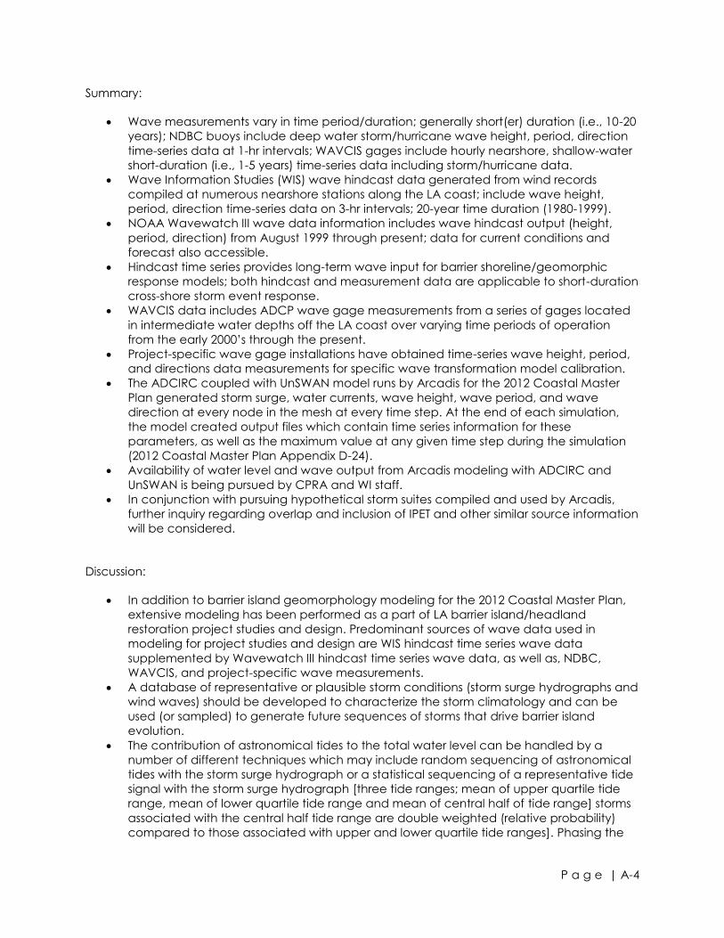
P a g e | A-4
Summary:
Discussion:
In addition to barrier island geomorphology modeling for the 2012 Coastal Master Plan,
extensive modeling has been performed as a part of LA barrier island/headland
restoration project studies and design. Predominant sources of wave data used in
modeling for project studies and design are WIS hindcast time series wave data
supplemented by Wavewatch III hindcast time series wave data, as well as, NDBC,
WAVCIS, and project-specific wave measurements.
A database of representative or plausible storm conditions (storm surge hydrographs and
wind waves) should be developed to characterize the storm climatology and can be
used (or sampled) to generate future sequences of storms that drive barrier island
evolution.
The contribution of astronomical tides to the total water level can be handled by a
number of different techniques which may include random sequencing of astronomical
tides with the storm surge hydrograph or a statistical sequencing of a representative tide
signal with the storm surge hydrograph [three tide ranges; mean of upper quartile tide
range, mean of lower quartile tide range and mean of central half of tide range] storms
associated with the central half tide range are double weighted (relative probability)
compared to those associated with upper and lower quartile tide ranges]. Phasing the
Wave measurements vary in time period/duration; generally short(er) duration (i.e., 10-20
years); NDBC buoys include deep water storm/hurricane wave height, period, direction
time-series data at 1-hr intervals; WAVCIS gages include hourly nearshore, shallow-water
short-duration (i.e., 1-5 years) time-series data including storm/hurricane data.
Wave Information Studies (WIS) wave hindcast data generated from wind records
compiled at numerous nearshore stations along the LA coast; include wave height,
period, direction time-series data on 3-hr intervals; 20-year time duration (1980-1999).
NOAA Wavewatch III wave data information includes wave hindcast output (height,
period, direction) from August 1999 through present; data for current conditions and
forecast also accessible.
Hindcast time series provides long-term wave input for barrier shoreline/geomorphic
response models; both hindcast and measurement data are applicable to short-duration
cross-shore storm event response.
WAVCIS data includes ADCP wave gage measurements from a series of gages located
in intermediate water depths off the LA coast over varying time periods of operation
from the early 2000’s through the present.
Project-specific wave gage installations have obtained time-series wave height, period,
and directions data measurements for specific wave transformation model calibration.
The ADCIRC coupled with UnSWAN model runs by Arcadis for the 2012 Coastal Master
Plan generated storm surge, water currents, wave height, wave period, and wave
direction at every node in the mesh at every time step. At the end of each simulation,
the model created output files which contain time series information for these
parameters, as well as the maximum value at any given time step during the simulation
(2012 Coastal Master Plan Appendix D-24).
Availability of water level and wave output from Arcadis modeling with ADCIRC and
UnSWAN is being pursued by CPRA and WI staff.
In conjunction with pursuing hypothetical storm suites compiled and used by Arcadis,
further inquiry regarding overlap and inclusion of IPET and other similar source information
will be considered.
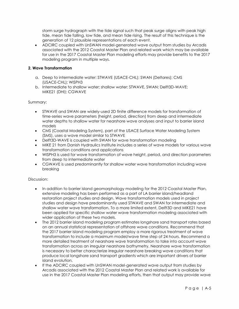
P a g e | A-5
storm surge hydrograph with the tide signal such that peak surge aligns with peak high
tide, mean tide falling, low tide, and mean tide rising. The result of this technique is the
generation of 12 plausible representations of each event.
ADCIRC coupled with UnSWAN model-generated wave output from studies by Arcadis
associated with the 2012 Coastal Master Plan and related work which may be available
for use in the 2017 Coastal Master Plan modeling efforts may provide benefits to the 2017
modeling program in multiple ways.
2. Wave Transformation
Summary:
Discussion:
In addition to barrier island geomorphology modeling for the 2012 Coastal Master Plan,
extensive modeling has been performed as a part of LA barrier island/headland
restoration project studies and design. Wave transformation models used in project
studies and design have predominantly used STWAVE and SWAN for intermediate and
shallow water wave transformation. To a more limited extent, Delft3D and MIKE21 have
been applied for specific shallow water wave transformation modeling associated with
wider application of these two models.
The 2012 barrier island modeling program estimates longshore sand transport rates based
on an annual statistical representation of offshore wave conditions. Recommend that
the 2017 barrier island modeling program employ a more rigorous treatment of wave
transformation to include a maximum model/wave time step of 24 hours. Recommend a
more detailed treatment of nearshore wave transformation to take into account wave
transformation across an irregular nearshore bathymetry. Nearshore wave transformation
is necessary to better characterize irregular nearshore breaking wave conditions that
produce local longshore sand transport gradients which are important drivers of barrier
island evolution.
If the ADCIRC coupled with UnSWAN model-generated wave output from studies by
Arcadis associated with the 2012 Coastal Master Plan and related work is available for
use in the 2017 Coastal Master Plan modeling efforts, then that output may provide wave
a. Deep to intermediate water: STWAVE (USACE-CHL); SWAN (Deltares); CMS
(USACE-CHL); WISPH3
b. Intermediate to shallow water; shallow water: STWAVE, SWAN; Delft3D-WAVE;
MIKE21 (DHI); CGWAVE
STWAVE and SWAN are widely-used 2D finite difference models for transformation of
time-series wave parameters (height, period, direction) from deep and intermediate
water depths to shallow water for nearshore wave analyses and input to barrier island
models
CMS (Coastal Modeling System), part of the USACE Surface Water Modeling System
(SMS), uses a wave model similar to STWAVE
Delft3D-WAVE is coupled with SWAN for wave transformation modeling
MIKE 21 from Danish Hydraulics Institute includes a series of wave models for various wave
transformation conditions and applications
WISPH3 is used for wave transformation of wave height, period, and direction parameters
from deep to intermediate water
CGWAVE is used predominantly for shallow water wave transformation including wave
breaking
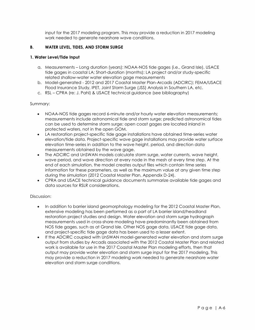
P a g e | A-6
input for the 2017 modeling program. This may provide a reduction in 2017 modeling
work needed to generate nearshore wave conditions.
B. WATER LEVEL, TIDES, AND STORM SURGE
1. Water Level/Tide Input
Summary:
Discussion:
a. Measurements – Long duration (years): NOAA-NOS tide gages (i.e., Grand Isle), USACE
tide gages in coastal LA; Short-duration (months): LA project and/or study-specific
related shallow-water water elevation gage measurements
b. Model-generated - 2012 and 2017 Coastal Master Plan-Arcadis (ADCIRC); FEMA/USACE
Flood Insurance Study, IPET, Joint Storm Surge (JSS) Analysis in Southern LA, etc.
c. RSL – CPRA (re: J. Pahl) & USACE technical guidance (see bibliography)
NOAA-NOS tide gages record 6-minute and/or hourly water elevation measurements;
measurements include astronomical tide and storm surge; predicted astronomical tides
can be used to determine storm surge; open coast gages are located inland in
protected waters, not in the open GOM.
LA restoration project-specific tide gage installations have obtained time-series water
elevation/tide data. Project-specific wave gage installations may provide water surface
elevation time-series in addition to the wave height, period, and direction data
measurements obtained by the wave gage.
The ADCIRC and UnSWAN models calculate storm surge, water currents, wave height,
wave period, and wave direction at every node in the mesh at every time step. At the
end of each simulation, the model creates output files which contain time series
information for these parameters, as well as the maximum value at any given time step
during the simulation (2012 Coastal Master Plan, Appendix D-24).
CPRA and USACE technical guidance documents summarize available tide gages and
data sources for RSLR considerations.
In addition to barrier island geomorphology modeling for the 2012 Coastal Master Plan,
extensive modeling has been performed as a part of LA barrier island/headland
restoration project studies and design. Water elevation and storm surge hydrograph
measurements used in cross-shore modeling have predominantly been obtained from
NOS tide gages, such as at Grand Isle. Other NOS gage data, USACE tide gage data,
and project-specific tide gage data has been used to a lesser extent.
If the ADCIRC coupled with UnSWAN model-generated water elevation and storm surge
output from studies by Arcadis associated with the 2012 Coastal Master Plan and related
work is available for use in the 2017 Coastal Master Plan modeling efforts, then that
output may provide water elevation and storm surge input for the 2017 modeling. This
may provide a reduction in 2017 modeling work needed to generate nearshore water
elevation and storm surge conditions.
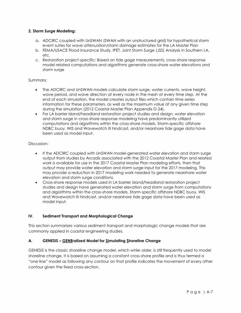
P a g e | A-7
2. Storm Surge Modeling:
Summary:
Discussion:
IV. Sediment Transport and Morphological Change
This section summarizes various sediment transport and morphologic change models that are
commonly applied in coastal engineering studies.
A. GENESIS – GENEralized Model for SImulating Shoreline Change
GENESIS is the classic shoreline change model, which while older, is still frequently used to model
shoreline change. It is based on assuming a constant cross-shore profile and is thus termed a
“one-line” model as following any contour on that profile indicates the movement of every other
contour given the fixed cross-section.
a. ADCIRC coupled with UnSWAN (SWAN with an unstructured grid) for hypothetical storm
event suites for wave attenuation/storm damage estimates for the LA Master Plan
b. FEMA/USACE Flood Insurance Study, IPET, Joint Storm Surge (JSS) Analysis in Southern LA,
etc.
c. Restoration project-specific: Based on tide gage measurements, cross-shore response
model related computations and algorithms generate cross-shore water elevations and
storm surge
The ADCIRC and UnSWAN models calculate storm surge, water currents, wave height,
wave period, and wave direction at every node in the mesh at every time step. At the
end of each simulation, the model creates output files which contain time series
information for these parameters, as well as the maximum value at any given time step
during the simulation (2012 Coastal Master Plan Appendix D-24).
For LA barrier island/headland restoration project studies and design, water elevation
and storm surge in cross-shore response modeling have predominantly utilized
computations and algorithms within the cross-shore models. Storm-specific offshore
NDBC buoy, WIS and Wavewatch III hindcast, and/or nearshore tide gage data have
been used as model input.
If the ADCIRC coupled with UnSWAN model-generated water elevation and storm surge
output from studies by Arcadis associated with the 2012 Coastal Master Plan and related
work is available for use in the 2017 Coastal Master Plan modeling efforts, then that
output may provide water elevation and storm surge input for the 2017 modeling. This
may provide a reduction in 2017 modeling work needed to generate nearshore water
elevation and storm surge conditions.
Cross-shore response models used in LA barrier island/headland restoration project
studies and design have generated water elevation and storm surge from computations
and algorithms within the cross-shore models. Storm-specific offshore NDBC buoy, WIS
and Wavewatch III hindcast, and/or nearshore tide gage data have been used as
model input.
P a g e | A-8
Methodology/Assumptions
Pros
Cons
B. LitPack
LitPack, developed by DHI, contains several modules within it to cover various coastal processes.
STP models non-cohesive sediment transport by waves and currents; LitDrift models longshore
currents and longshore transport; LitLine addresses coastal evolution.
Methodology
Pros
Cons
Beach profile shape is constant (1D model)
Seaward and shoreward limits of profile are constant
Longshore sand transport is due to wave action
Finite difference solution scheme using Crank-Nicholson implicit scheme
Classic methodology for simulating shoreline changes based on wave input and
sediment transport rate equations
Widely used and tested methodology
Relatively simple in terms of coding
Can handle long-term simulations (decadal)
Critical input available from USACE
Can’t handle fundamental change in composition of beach face (i.e. switching
percentage of silt and sand in the beach face that occurs in Louisiana when a barrier
island is restored
Manual adjustments needed to account for overwash and lowering of berm/dune
elevation observed in Louisiana following large storm events
Doesn’t handle sand loss to inlets or tidal current driven transport
Doesn’t account for offshore loss of silt due to suspension
One line model doesn’t allow for acreage calculations or overwash benefits
Not open source
Model basis is turbulent wave-current boundary layer (Fredsoe, 1984).
Interpolation and finite difference techniques
Solves basic continuity equation
Can handle suspended sediment
Widely used and tested methodology
Relatively simple in terms of coding
Not open source
One line model doesn’t allow for acreage calculations or overwash benefits
Unclear as to run time for long term simulations
Unclear as to how it can deal with overwash and lowering of dune
P a g e | A-9
C. AdH Model
The ADH model was developed by USACE ERDC. It adds a time varying component capability
to ADCIRC and STWAVE and can be used in conjunction with the Surface Water Modeling
System (SMS) as a pre- and post-processor.
Methodology
Pros
Cons
D. Delft3D
Delft3D is one of the more advanced three-dimensional models on the market for modeling
coastal processes. It is a three dimensional model and can track morphologic change over
entire basins and even the State depending on grid size and computing power. It has multiple
modules to deal with wave transformation (SWAN). It has recently opened the code though the
GUI must still be purchased.
Methodology
Unstructured finite element mesh, which can be dynamically refined in areas where
more resolution is needed.
Quasi-3D shallow water hydrodynamically driven model using 2D shallow water
equations.
Probabilistic representation of sediment transport that includes wave and current
transport of bed and suspended load.
Critical input/technical support available from USACE.
Can handle transport of mixed sediment systems (sand and clays)
Incorporates many of the complex coastal processes required to predict overtopping,
longshore transport and losses
Integration with other portions of the 2017 Coastal Master Plan model could be difficult.
Limited duration of modeled period (1-2 years) because computationally intensive
Linkage with STWAVE only available in beta version at present time.
Open source?
Finite difference model that can be run in full 3D, 2D-H, or 2D-V mode.
Incorporates majority of coastal processes related to waves, winds, currents, water levels,
and sediment transport.
Relies on a morphologic factor (morfac) to decrease computing time. The morfac
equals the length of the study period x percent occurrence for each wave case/
duration of the wave case in the model simulation.

P a g e | A-10
Pros
Cons
E. MIKE-21 and MIKE-3
MIKE-21 and MIKE-3 were developed by DHI. As with other complex models, it is composed of
several modules that examine wave transformation (SW), sediment transport
Methodology
Pros
Cons
F. SBEACH
SBEACH (Storm-induced BEAch CHange model) was developed by the USACE and is operated
within the CEDAS user interface. It is a cross-shore, 2D model that models cross-shore
morphologic response in response to a storm event based on measurement derived, empirical
equations. It is a widely used model that has been applied extensively in coastal Louisiana to
estimate dune lowering and overwash extents across barrier islands.
Incorporates many of the complex coastal processes required to predict overtopping,
longshore transport and losses
Morphologic model that can account for islands, bays and inlets.
Can model long durations (several years to decades) due to the application of the
morfac.
Can handle mixed sediment systems though it drives computing time up.
Integration with other portions of the 2017 Coastal Master Plan model could be difficult.
Computationally intensive with very long run times
Does not include subaerial rebuilding resulting in continued island elevation loss over
time.
Not a model upon which we could base our code.
Does not allow unstructured grid, which is better suited for irregular coastlines.
Model basis is spectral wave and radiation stress.
Uses mean horizontal velocities and radiation stress to drive bed load sediment transport
and
Solves basic continuity equation.
Morphologic change model that can account for islands, bays and inlets.
Can handle suspended sediment and
Widely used and tested methodology
Relatively simple in terms of coding
Not open source
Limited model duration 1-2 years
Unclear as to how it can deal with overwash and lowering of dune
P a g e | A-11
Methodology
Pros
Cons
G. Beach-fx
Beach-fx was developed by the USACE as an engineering-economic planning tool. Essentially, it
greatly expands upon a single SBEACH run at a single profile to thousands of storm events along
multiple profiles and combines them with upland property value to estimate damage values.
This probabilistic outcome is an improvement upon the single storm outcome of SBEACH but
increases computational time.
Methodology
The model is based on equation of mass conservation and uses empirical relationships
derived from measurements.
Contains a wave transformation component that is based on small amplitude wave
theory up to breaking and then the breaker decay model (Dally, 1980).
Assumes that there is no gradient in longshore transport (essentially ignoring longshore
transport).
It is uses Fortran 77 and C++ programming languages.
Widely used and recognized model. Calibration parameters are readily available.
Relatively quick to perform a storm run with easy input and output parameters.
Variable grid available to allow more detailed elevation following in swash and
overwash zones.
Critical input available from USACE.
Not open source.
Doesn’t have island elevation rebuilding mechanism during quiescent periods beyond
the wave runup limit.
Doesn’t account for mixed sediment system that is being eroded. It has been observed
that there is a sandy veneer along Louisiana’s barrier islands. This is overwashed during
storm events exposing the cohesive mixed sediments that can survive storm. However,
regular wave action then erodes the beach face, reforming the sandy veneer in the
weeks to months following the storm event (Campbell, 2005).
Doesn’t account for change in material at the commonly observed break in slope on
profiles west of the river. Above this elevation (typically -1.2 to -2.1 meters, NAVD) the
material is sandy while below this elevation the sediment is typically composed of silt and
clay. This does not appear to be a critical issue given the flat offshore slopes initiate
breaking and have a wide breaker zone except that it excludes wave damping by a
fluid mud layer.
Cross-shore results use SBEACH as underlying coastal engineering model but enhanced
with an event based Monte Carlo life-cycle simulation of storm events.
An MS Access database builds in upland infrastructure information with a GIS and GUI
interface.
P a g e | A-12
Pros
Cons
H. EDUNE
EDUNE was developed by Dave Kriebel (with Robert Dean an early collaborator). It is a cross-
shore, 2D model that is based on Dean’s equilibrium profile theory and uses a finite difference
solution.
Methodology:
Pros
Cons
I. Coastal Planning & Engineering (CPE) In-house Analytic Model
CPE has applied an in-house model to estimate shoreline and acreage changes over decadal
time periods. It is an MS-Excel based analytic model based on averaging shoreline retreat rates
and a single storm event history.
As storm response is based on the SBEACH model, the positive aspects of the SBEACH
model are achieved.
It takes the single SBEACH run and develops a Monte Carlo simulation of runs to
determine a probabilistic outcome rather than single result.
The damage portion of the program is not required for the work that is proposed for the
2017 Coastal Master Plan.
As storm response is based on the SBEACH model, the drawbacks are similar.
Storm damages are not sequential (i.e. a 5-year storm following a 20-year storm). Given
the sensitivity of Louisiana barrier islands to overtopping this is concern.
To apply a Monte Carlo simulation of storm events requires that 50-year runs be
performed with integration of longshore components on an annual basis. Computing
time for this approach is increased.
Open source?
Based on Dean’s equilibrium profile theory and solving for energy dissipation.
Relatively quick and easy to apply.
Open source
Developed for the case of high dunes that extend infinitely landward and thus does not
include the major coastal process of overwash that drives Louisiana barrier island
morphology change.
Requires external wave transformation model to provide breaking wave height though
sediment transport is based on exceeding the equilibrium dissipation
P a g e | A-13
Methodology
Pros
Cons
Discussion of Sediment Transport and Morphologic Change
A simple one-line model is insufficient to meet the expectations of CPRA. While a comprehensive
3D model would provide the most robust solution, it is unlikely that a full 3D model could be
developed within the timeline required for enhancement of the barrier island modeling task. Run
times for these types of models can also be excessive, which makes them impractical for the 50-
year predictions that CPRA is seeking. Combing a 2D longshore model and 2D cross-shore event
storm event driven model is an achievable goal and could meet CPRA’s expectations.
Most of the models include a GUI (graphic user interface). Given that a commercial model is not
required, this should not be a requirement of the modeling team. More importantly, it may allow
CPRA to request the underlying code driving the coastal engineering principles, if it is not
already open source. This could save considerable time and improve the final model by
allowing time to be focused on revising, integrating and testing the model code rather than
starting from the beginning.
None of the models reviewed incorporate subaerial rebuilding due to aeolian transport. Given
the relationship between overwash and island elevation, this process should be incorporated
into the BIMODE modeling effort.
Most of the reviewed models cannot effectively handle mixed sediment systems, such as occurs
along coastal Louisiana.
Spreadsheet based, analytic model accounting for multiple coastal processes
Based on average conditions of shoreline (gulf and bay) retreat, RSLR, etc., except for
discrete storm events causing overwash and lowering of the dune
Incorporates cross-shore modeling from SBEACH
Easy to follow, explain and incorporate additional processes
Easy to update for various islands under with and without project conditions (change in
sand content)
Provides acreage and shoreline length outputs
Can be readily adapted to a Fortran code
Not a peer reviewed model
Doesn’t directly incorporate waves and tides or fundamental coastal equations into the
model
Extrapolates averaged conditions to a longer timescale
Limited to single island runs and doesn’t account for inlet processes
P a g e | A-14
V. Tidal Inlets and Estuaries/Bays
This section summarizes various models capable of simulating estuarine circulation, sediment
transport, and associated inlet processes that are commonly applied in coastal engineering
studies.
A. AdH Model
The ADH model was developed by USACE ERDC. It adds a time varying component capability
to ADCIRC and STWAVE and can be used in conjunction with the Surface Water Modeling
System (SMS).
Methodology
Pros
Cons
B. Delft3D
Delft3D is one of the more advanced three-dimensional models on the market for modeling
coastal processes. It is a three-dimensional model and can track morphologic change over
entire basins and even the State depending on grid size and computer power. It has multiple
modules to deal with wave transformation (SWAN), hydrodynamics (FLOW), and sediment
transport (MORPHO). Although the code has recently been opened, the GUI source remains
closed.
Unstructured finite element mesh, which can be dynamically refined in areas where
more resolution is needed.
Quasi-3D shallow water hydrodynamically driven model using 2D shallow water
equations.
Probabilistic representation of sediment transport that includes wave and current
transport of bed and suspended load.
Critical input available from USACE.
Can handle transport of mixed sediment systems (sand and clays)
Incorporates many of the complex coastal processes required to predict overtopping,
longshore transport and losses
Adaptive mesh improves computational efficiency
Integration with other portions of the Master Plan model could be difficult.
Limited duration of modeled period (1-2 years)
Linkage with STWAVE only available in beta version at present time.
Open source?
P a g e | A-15
Methodology
Pros
Cons
C. MIKE-21 and MIKE-3
MIKE-21 and MIKE-3 were developed by DHI. As with other complex models, it is composed of
several modules that examine wave transformation (SW), hydrodynamic module (HD), and the
sand and mud transport modules (ST and MT).
Methodology:
Pros
Widely used and tested methodology.
Finite difference model that can be run in full 3D, 2D-H, or 2D-V mode.
Incorporates majority of coastal processes related to waves, winds, currents, water levels,
and sediment transport.
Relies on a morphological acceleration factor (MORFAC) to decrease computing time.
The morphological acceleration factor is a factor, which multiplies the bathymetric and
topographic changes in a given time step, so that, for example, a 14 day model
simulation can be used to simulate 1 year of bathymetric and topographic changes. In
this particular example, a 14 day simulation with a MORFAC of 26 can be used to
simulate 1 year of bathymetric change (26 = 365/14).
Incorporates many of the complex coastal processes required to predict overtopping,
longshore transport and losses
Morphologic model that can account for islands, bays and inlets.
Can model long durations (several years to decades) due to the application of the
morfac.
Can handle mixed sediment systems though it increases computing time.
Integration with other portions of the Master Plan model could be difficult.
Computationally intensive with very long run times.
Does not include subaerial rebuilding resulting in continued island elevation loss over
time.
Not a model upon which we could base our code.
The SWAN model, which is the companion wave transformation model for Delft3D, has
been judged by some experts to be computationally slow (William Dally, 2012, pers.
comm.).
Model basis is spectral wave and radiation stress.
Uses mean horizontal velocities and radiation stress to drive bed load sediment transport
and
Solves basic continuity equation.
Optional unstructured finite element mesh, which can be refined in areas where more
resolution is needed.
Morphologic change model that can account for islands, bays and inlets.
Can compute suspended sediment.
P a g e | A-16
Cons
D. ECOMSED/EFDC/FVCOM/RMA2/3 others
These are from the family of estuarine models that can address hydrodynamics and salinity and
temperature transport, and some of them can also address tracers and sediment. All these
models are similar in capability to Delft3D and they are rather advanced two- and three-
dimensional models. Although sediment transport with mobile bed options is available in most of
these models, they do not have the advantage of morphological upscaling (similar to Delft3D)
and hence are relatively slow.
Methodology
Pros
Can handle mixed sediment systems though it increases computing time.
Cons
E. ASMITA or similar
This is a simple box-type model that treats the basin, tidal flats, inlets, and coastal ocean in a
dynamic way. Because it lacks sufficient spatial resolution, this model cannot be used to infer
circulation patterns within an estuary or bay, but can sufficiently and accurately help infer tidal
prism changes over long periods, because of its short execution times (for simulations over
centuries).
Methodology
MIKE21SW wave model has a fast and computationally efficient solution scheme.
A new version of the MIKE21/MIKE3 flow model has been introduced to run on the GPU
cards developed for video games. This could speed up run time substantially (Mikkel
Andersen, 2013, pers. comm.)
Not an open source.
In the traditional, CPU version, the model duration is limited to 1-2 years due to strictly
sequential wave forcing
Unclear as to how it can deal with overwash and lowering of dune during storms
Finite difference, finite element and/or finite volume in 3D or 2D modes.
Incorporate majority of coastal processes related to waves, winds, currents, water levels,
and sediment transport.
Integration with other portions of the Master Plan model could be difficult.
Computationally intensive with very long run times
Finite difference methods (largely ordinary linear differential equations)
Can incorporate or address major exchange processes between the ocean and bay
(and hence basic hydraulics at inlets connecting the two basins.

P a g e | A-17
Pros
Cons
F. Link node models (also known as box models)
Similar to ASMITA these models are very similar to those used by the eco-hydrology team in the
2012 Coastal Master Plan. Because they have reduced spatial resolution, they can run much
faster and represent bulk processes (such as tidal propagation and other constituent transport
through a basin).
Methodology
Pros
Cons
G. Simple inlet equilibrium relationships
These are simple algebraic equations based on the work of Jarrett (1976) and O’Brien (1931,
1969). Input to these models is the tidal prism and the result or output is inlet geometry (i.e., inlet
throat cross-sectional area).
Methodology
Simple algebraic equations
Runs quickly
Good estimate of the tidal prism changes over time
Tracks estuarine depth, and tidal flat and marsh elevation, and hence can account for
tidal prism in a dynamic way.
Lack of spatial resolution
Could misrepresent circulation patterns (if needed or required)
Likely ignores short duration events, such as entrainment of sediment from individual
storms, or wind driven effects on the estuary/bay circulation.
Ignores sub-grid scale inlet processes
Finite difference methods (largely ordinary linear differential equations)
Can incorporate or address major processes
Runs quickly
Good estimate of the tidal prism changes over time
Lack of spatial resolution
Could misrepresent circulation patterns
Ignores sub-grid scale inlet processes
P a g e | A-18
Pros
Cons
H. Simple 1-D inlet hydrodynamics
These models are analytical or numerical solutions of inlet hydrodynamic and resulting bay –
ocean exchange, with the objective of predicting inlet morphologic evolution.
Methodology
Using knowledge of tides at the ocean, these models use pressure gradient calculations,
and density gradient effects to estimate flux of water and mass through inlet for a
desired period.
Pros
Cons
** The above models have different capabilities and limitations and there are others that have
similar application that have not been discussed.
Discussion of Processes at Inlets and Estuaries (that models should account for)
Inlet hydrodynamics
Knowledge of inlet hydrodynamics is critical to determine whether inlets will remain open,
enlarge, or close, because of insufficient current to transport sediment through the inlet. Current
models in the 2012 Coastal Master Plan do not provide detail hydrodynamics, although a single
velocity for every time-step is known and can be used if needed. This information may also be
important in determining the ebb-jet size and structure and perhaps help with additional
information regarding sediment transport in the vicinity of the inlet.
Runs quickly
Good estimate of the inlet cross-sectional due to a change in the tidal prism over time
Lack of spatial resolution
Ignores sub-grid scale inlet processes
Often run relatively quickly, because they only consider standardize idealized areas
rather than specific geographic areas.
Good estimate of the inlet cross-sectional area change, because of a change in the
tidal prism over time
May provide additional information on velocity variation at inlet, and perhaps better
infer inlet morphology.
Lack of spatial resolution
Ignores sub-grid scale inlet processes as well as estuary processes.

P a g e | A-19
Inlet morphology
One requirement for assessing the dynamics of an inlet’s cross-sectional area is knowledge of its
tidal prism. If known, then the inlet can be adjusted using a minimum equilibrium cross section
given by relationship (Jarret 1976, and O’Brien, 1931; 1969). This code was performed for the 2012
Coastal Master Plan, but the inlets were static in time. However, information from the ocean-
estuary exchange can be used to infer these processes further, and assist in determining
morphological evolution at more frequent time-steps using more process-based variables, such
as shear velocity.
A challenging scenario would be the case where inlets open or barriers breach during storms
(assuming that the new barrier models can predict that). It will be important to pass this
information to the eco-hydrology teams who deal with estuary processes, but we note that this is
a challenging step, because the links representing inlets in those models are held constant in
time (i.e. no new inlets will be allowed once the simulation begins).
Interaction of Inlets with nearby environments
Obviously, since inlets connect the coastal ocean and interior bays, any model used to assess
this interaction must be at least able to force exchange caused by pressure gradients across the
inlet. Most models, including current 2012 Coastal Master Plan eco-hydrology models, can
already address this. This computation is critical for calculating tidal prism. In the 2012 modeling
program this calculation was done using maximum monthly tidal range multiplied by the area of
the corresponding box, and integrated across the entire basin to compute the tidal prism.
Whatever tool exists for the 2017 modeling program must be able to address at least this step,
but doing so more frequently so that the process of inlet expansion/enlargement is coupled.
Inlets are often associated with ebb (and/or flood) deltas. Knowledge of ebb delta morphology
and dimensions is critical for correctly interpreting processes in the nearshore environments near
barriers. For example, sediment bypassing is a process associated with inlets; however, ebb
deltas often control the temporal and spatial aspects of sediment bypassing inlets and impose
additional sediment sinks/sources that could significantly affect the longshore sediment transport
budget. It is recommended that some of these processes are included in the barrier model for
more realistic representation of the system.
In Louisiana, there are several inlets that are not well defined; they are transgressive systems and
tend to be wave influenced and storm-dominated. These inlets are especially important for
several reasons. First, although they are rather large inlets (3-5 km across), they have a narrow
active channel and thalweg (1-2 km) and flanked on one or both sides by a shallower platform.
The flow dynamics of the thalweg and adjacent platform areas have significant influence on
sediment transport (both alongshore and cross-shore), and something that can critically affect
barrier island evolution.
The shoreface fronting barriers in Louisiana are highly erosional and in disequilibrium with the
wave energy exhibited by large sediment deficits, which believed to be caused by storms. These
areas are well beyond closure depths, and therefore if there is interest to include this process in

P a g e | A-20
the 2017 modeling program, additional routines (or perhaps extending the cross-shore profiles
farther offshore) must be considered to account for this trend.
Estuarine hydrodynamics or circulation
Estuarine circulation can be determined by many of the models presented herein and, to some
extent, by models currently available from the 2012 Coastal Master Plan. Assuming that the
approach remains the same for 2017 Coastal Master Plan for estuaries, the inlets should be
coupled with the estuary models on a standard basis, such that updates on inlet morphology
(cross-sectional area) as a minimum are transferred back to the estuary models immediately
(during the 2012 modeling program this was done every 25 years, but doing so every year will be
beneficial).