Embed Size (px)
Citation preview

Coastal Protection and Restoration Authority 150 Terrace Avenue, Baton Rouge, LA 70802 | [email protected] | www.coastal.la.gov
2017 Coastal Master Plan
Attachment C3-24:
Integrated Compartment
Model Uncertainty Analysis
Report: Final
Date: April 2017
Prepared By: Ehab Meselhe, Eric White, Yushi Wang (The Water Institute of the Gulf)

2017 Coastal Master Plan: ICM Uncertainty Analysis
Page | ii
Coastal Protection and Restoration Authority
This document was prepared in support of the 2017 Coastal Master Plan being prepared by the
Coastal Protection and Restoration Authority (CPRA). CPRA was established by the Louisiana
Legislature in response to Hurricanes Katrina and Rita through Act 8 of the First Extraordinary
Session of 2005. Act 8 of the First Extraordinary Session of 2005 expanded the membership, duties,
and responsibilities of CPRA and charged the new authority to develop and implement a
comprehensive coastal protection plan, consisting of a master plan (revised every five years)
and annual plans. CPRA’s mandate is to develop, implement, and enforce a comprehensive
coastal protection and restoration master plan.
Suggested Citation:
Meselhe, E.M, White, E.D., and Wang, Y. (2017). 2017 Coastal Master Plan: Attachment C3-24:
Integrated Compartment Model Uncertainty Analysis. (pp. 1-68). Baton Rouge, Louisiana:
Coastal Protection and Restoration Authority.

2017 Coastal Master Plan: ICM Uncertainty Analysis
Page | iii
Acknowledgements
This document was developed as part of a broader Model Improvement Plan in support of the
2017 Coastal Master Plan under the guidance of the Modeling Decision Team (MDT):
The Water Institute of the Gulf - Ehab Meselhe, Alaina Grace, and Denise Reed
Coastal Protection and Restoration Authority (CPRA) of Louisiana - Mandy Green,
Angelina Freeman, and David Lindquist
This effort was funded by the Coastal Protection and Restoration Authority (CPRA) of
Louisiana under Cooperative Endeavor Agreement Number 2503-12-58, Task Order No.
03.
2017 Coastal Master Plan: ICM Uncertainty Analysis
Page | iv
Executive Summary
In long-term coastal planning efforts, especially one as critical as Louisiana’s coastal master
plan, it is important to consider the effects of uncertainties on predicted outcomes. To build
upon the 2012 Coastal Master Plan modeling effort, the approach described herein provides a
framework to perform the uncertainty analysis (UA).
A coast wide Integrated Compartment Model (ICM) has been developed as a landscape
model for use in the 2017 Coastal Master Plan. It includes hydrology, water quality, morphology,
vegetation, barrier islands, and habitat suitability indices. In the modeling effort of the 2017
Coastal Master Plan, two primary sources of uncertainties were investigated. First is the
uncertainty in the environmental drivers, namely, eustatic sea level rise, subsidence,
precipitation, and evapotranspiration. This uncertainty was addressed through an environmental
scenario approach, where the modeled landscape response was evaluated across different
combinations of values for these environmental drivers (Appendix C: Chapter 2). The second
source of uncertainty investigated is associated with the calculations of critical model variables
and how they influence key model output. This component of the UA is the focus of this report.
The main objective of this analysis is to quantify the magnitude of the uncertainty in key model
output driven by uncertainties in critical model variables. Land area was identified as the key
model output for the analysis. The analysis performed here is applied to the validated Future
Without Action (FWOA) ICM model simulation, also referred to here as the base case.
The uncertainty analysis approach utilized in this report was based on applying perturbations to
model variables that are directly linked to the calculations of land area. The model variables
examined include water level, salinity, wetland types, suspended mineral sediment
concentration, and organic accretion. The magnitudes of the perturbations were estimated
based on the calibration errors and were then applied annually and for the duration of the 50-
year simulations.
The perturbations were initially applied individually to identify which model variables had
significant impacts on land area. The individual perturbations showed that water level and
organic accretion have the most influence on land area. Salinity, while having an influence on
the wetland type, did not have significant impact on land area. Land area was also not
impacted significantly by total suspended sediment. Perturbations to predicted areas of
different wetland types were not included here as they were controlled by the prevailing
hydrologic conditions. As such, the uncertainty in land area, as determined by wetland type,
was determined indirectly via perturbations to hydrologic conditions, and as such, uncertainties
due to vegetation type were removed from further consideration.
The uncertainty range resulting from linearly adding the uncertainty of the individual
perturbations was compared to the outcome of a set of 16 permutations designed to examine
the interdependency among the uncertainty of the model variables. The comparison showed
that the uncertainty range resulting from the 16 permutation composite set was wider than the
linearly added uncertainty bracket. This outcome demonstrates that interdependency among
the model variables is important. The results of the composite experiments show that water level,
organic accretion, and their interdependence are the most influential on coast wide land area.
The 16 permutations of composite perturbations were performed for the high scenario FWOA for
both ICM_v1 and ICM_v3, which were model settings used for individual project-level analyses
and alternative/plan-level analyses conducted for the 2017 Coastal Master Plan, respectively.
The 16 uncertainty permutations were also performed on the Draft 2017 Coastal Master Plan
under the high scenario. In general, model prediction uncertainty decreased over time under

2017 Coastal Master Plan: ICM Uncertainty Analysis
Page | v
the high scenario FWOA due to relative sea level rise rates which overwhelmed the uncertainty
introduced by the perturbed model output variables. Regardless of the perturbations performed
for each permutation, the coast wide land area asymptotically approached the same lower
limit in all permutations over time. With the Draft 2017 Coastal Master Plan implemented, the
land area no longer approached this lower limit under the high scenario. This resulted in more
uncertainty due to the presence of more land being present within the model domain in later
decades. Spatial analysis of the model uncertainty presented here shows that the most
uncertain areas within the model fall outside of the project footprint areas. This indicates a
reasonable level of confidence in the primary land change numbers predicted by ICM during
the 2017 Coastal Master Plan analysis.
Throughout all of the uncertainty analysis runs conducted, the total range of land area was 9,400
km2 to 14,000 km2, with a baseline prediction of 11,700 km2 under the low scenario FWOA using
ICM_v1. Under the high scenario, using ICM_v1, the land area ranged from 4,000 km2 to 8,200
km2, with a baseline prediction of 5,300 km2. Under the high scenario, using ICM_v3, the land
area ranged from 4,000 km2 to 8,700 km2, with a baseline prediction of 5,600 km2. Finally, under
the high scenario using ICM_v3, the Draft 2017 Coastal Master Plan land area ranged from 6,800
km2 to 11,300 km2, with a baseline prediction of 8,600 km2.
Many model input parameters were not able to be perturbed by the methodology followed for
the uncertainty analysis, in which model performance errors were used to assign a perturbation
factor to model outputs. The modeling team determined that the ICM prediction of land area at
year 50 seemed to be particularly sensitive to three such parameters: subsidence rates, organic
matter accretion, and marsh collapse threshold values. The spatial extent of model-predicted
land area changed substantially due to setting these variables at extreme values. Of the marsh
collapse threshold values, the year 50 prediction of land area within the model domain was
most sensitive to the saline marsh inundation-induced collapse threshold; a finding in agreement
with the fact that the majority of land remaining at year 50 under the medium scenario is saline
marsh. The extent of land impacted by the total range tested in subsidence rates and organic
matter input rates were roughly the same magnitude as the saline marsh collapse threshold. The
land area predicted at year 50 was not as sensitive to collapse thresholds for brackish,
intermediate, or fresh marsh types.

2017 Coastal Master Plan: ICM Uncertainty Analysis
Page | vi
Table of Contents
Coastal Protection and Restoration Authority ............................................................................................ ii
Acknowledgements ......................................................................................................................................... iii
Executive Summary ......................................................................................................................................... iv
Table of Contents ............................................................................................................................................. vi
List of Tables ...................................................................................................................................................... vii
List of Figures ..................................................................................................................................................... vii
List of Abbreviations ......................................................................................................................................... ix
1.0 Introduction ............................................................................................................................................... 1 1.1 Rationale and Background ................................................................................................................... 1 1.2 Terminology ............................................................................................................................................... 2
2.0 Approach .................................................................................................................................................. 2 2.1 Overview of 2012 Coastal Master Plan Uncertainty Analysis .......................................................... 2 2.2 Uncertainty Analysis Approach for the Integrated Compartment Model ................................... 3
3.0 Methodology ............................................................................................................................................ 5 3.1 Estimating the Perturbation Terms for Water Level, Salinity, and Total Suspended Solids ......... 7 3.2 Estimating the Perturbation Terms of Wetland Types ........................................................................ 8 3.3 Estimating the Perturbation Terms for Organic Loading .................................................................. 9
4.0 Experimental Design and Results – Phase 1 ........................................................................................ 9 4.1 Salinity Analysis ....................................................................................................................................... 12 4.2 Water Level Analysis .............................................................................................................................. 13 4.3 Total Suspended Solids Analysis .......................................................................................................... 17 4.4 Organic Sediment Analysis .................................................................................................................. 18 4.5 Composite Experiments ........................................................................................................................ 20
5.0 Spatial Analysis of Uncertainty – Phase 1 .......................................................................................... 21
6.0 Assessing Future Without Action Model Uncertainty (High Scenario) – Phase 2 ....................... 26 6.1 Methodology for Assessing Spatial Patterns of Uncertainty – Phase 2 ........................................ 26 6.2 Comparison Between Low and High Scenarios .............................................................................. 27 6.3 Comparison Between ICM Versions 1 and 3 .................................................................................... 29
7.0 Assessing Model Uncertainty Under the Future With Action Draft Master Plan ......................... 31 7.1 Spatial Patterns of Future With Draft Master Plan Uncertainty ...................................................... 31 7.2 Magnitude and Temporal Behavior of Uncertainty ........................................................................ 33
8.0 Additional Model Sensitivity Analysis .................................................................................................. 48 8.1 Model Sensitivity to Organic Accretion Input Data ........................................................................ 48 8.2 Model Sensitivity to Subsidence Rates ............................................................................................... 49 8.3 Model Sensitivity to Marsh Collapse Thresholds ............................................................................... 52
9.0 Summary and Conclusions .................................................................................................................. 57
10.0 References ............................................................................................................................................ 59

2017 Coastal Master Plan: ICM Uncertainty Analysis
Page | vii
List of Tables
Table 1: Error terms from the hydrology subroutine calibration period used to perturb the
Integrated Compartment Model. (See Appendix C-23: ICM Calibration and Validation for error
terms and discussion.) ...................................................................................................................................... 8
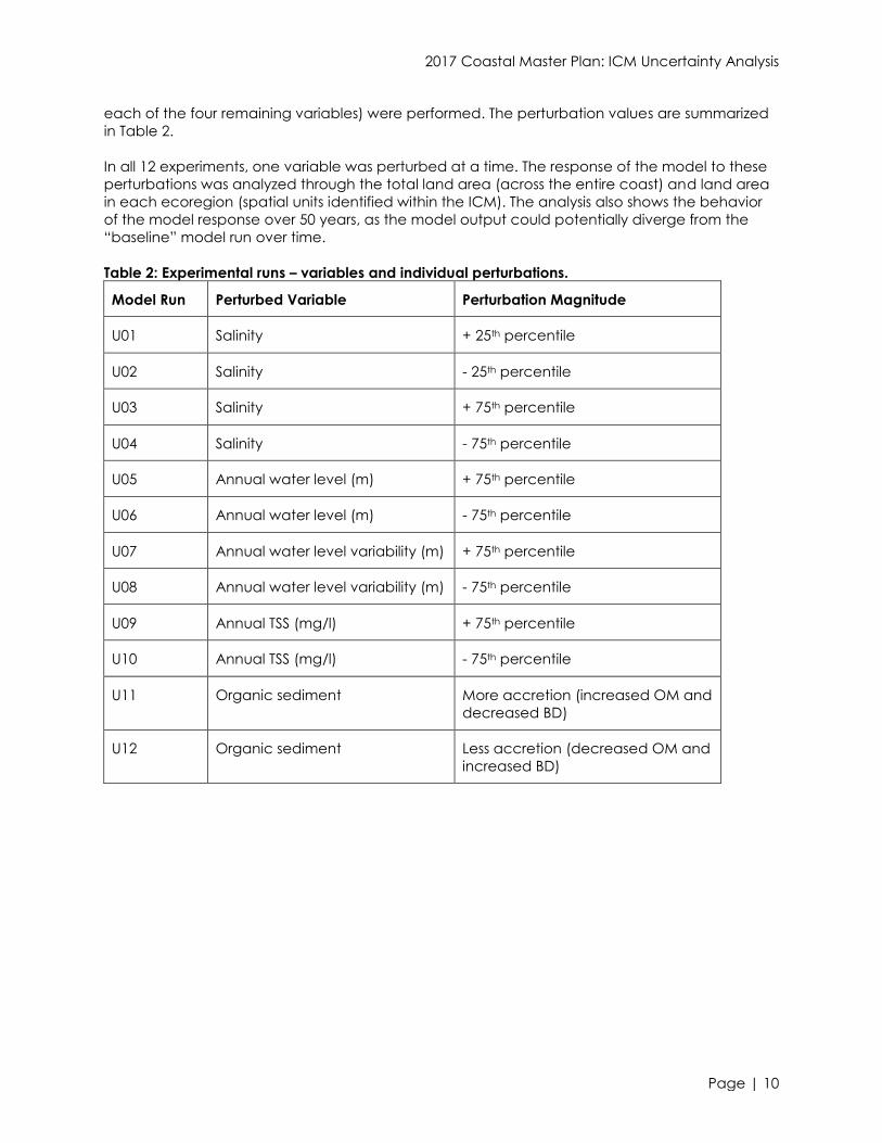
Table 2: Experimental runs – variables and individual perturbations. ................................................... 10
Table 3: Composite experimental runs. ...................................................................................................... 20
Table 4: Experimental runs – composite perturbations – all permutations. .......................................... 23
Table 5: Inundation collapse thresholds used to assess model sensitivity. ........................................... 53
List of Figures
Figure 1: Conceptual diagram for Phase 1 parametric uncertainty approach. ................................. 6
Figure 2: Total land change over time for U01.. ........................................................................................ 11
Figure 3: Total land change over time for U02.. ........................................................................................ 11
Figure 4: Total land change over time for U03.. ........................................................................................ 12
Figure 5: Total land change over time for U04.. ........................................................................................ 13
Figure 6: Total land change over time for U05.. ........................................................................................ 14
Figure 7: Total land change over time for U06.. ........................................................................................ 14
Figure 8: Total land change over time for U07.. ........................................................................................ 15
Figure 9: Total land change over time for U08.. ........................................................................................ 15
Figure 10: Relative abundance of vegetation types over the 50-year simulation ............................. 16
Figure 11: Total land change over time for U09 ........................................................................................ 17
Figure 12: Total land change over time for U10 ........................................................................................ 18
Figure 13: Total land change over time for U11 ........................................................................................ 19
Figure 14: Total land change over time for U12 ........................................................................................ 19
Figure 15: Total land change over time for U21 (green line) and U22 (red line) ................................ 21
Figure 16: Land/water prediction uncertainty – all individual perturbations at year 50. .................. 22
Figure 17: Land/water prediction uncertainty – all individual perturbations and composite run
U22 (near Myrtle Grove, year 50). ................................................................................................................ 23
Figure 18: Land/water prediction uncertainty – composite perturbations with (U22) and without
perturbed TSS (U31); near Davis Pond, year 50. ........................................................................................ 25
Figure 19: Baseline FWOA land area over time (U00, black line) compared against all 16
permutations of composite uncertainty perturbations. .......................................................................... 26
Figure 20: Relative uncertainty in baseline FWOA predictions under the low scenario using version
1 of the ICM (S01 G001). ................................................................................................................................ 28

2017 Coastal Master Plan: ICM Uncertainty Analysis
Page | viii
Figure 21: Relative uncertainty in baseline FWOA predictions under the high scenario using
version 1 of the ICM (S03 G001). .................................................................................................................. 29
Figure 22: Relative uncertainty in baseline FWOA predictions under the high scenario using
version 3 of the ICM (S03 G300). .................................................................................................................. 30
Figure 23: Relative uncertainty in baseline Future With Draft Master Plan predictions under the
high scenario using version 3 of the ICM (S03 G400). .............................................................................. 32
Figure 24: Range in coast wide land area prediction from all permutations under low scenario.. 33
Figure 25: Land area change over time for total model domain area ............................................... 35
Figure 26: Land area change over time for Upper Pontchartrain (UPO) Ecoregion ......................... 36
Figure 27: Land area change over time for Lower Pontchartrain (LPO) Ecoregion .......................... 37
Figure 28: Land area change over time for Breton (BRT) Ecoregion .................................................... 38
Figure 29: Land area change over time for Bird’s Foot Delta (BFD) Ecoregion .................................. 39
Figure 30: Land area change over time for Upper Barataria (UBA) Ecoregion .................................. 40
Figure 31: Land area change over time for Lower Barataria (LBA) Ecoregion ................................... 41
Figure 32: Land area change over time for Lower Terrebonne (LTB) Ecoregion ................................ 42
Figure 33: Land area change over time for Atchafalaya/Teche/Vermilion (AVT) Ecoregion......... 43
Figure 34: Land area change over time for Mermentau/Lakes (MEL) Ecoregion .............................. 44
Figure 35: Land area change over time for Calcasieu/Sabine (CAS) Ecoregion .............................. 45
Figure 36: Land area change over time for Eastern Chenier Ridge (ECR) Ecoregion ...................... 46
Figure 37: Land area change over time for Western Chenier Ridge (WCR) Ecoregion ................... 47
Figure 38: All land under low scenario FWOA using ICM_v1 that is sensitive to individual
perturbation of organic accretion inputs ................................................................................................... 49
Figure 39: Sensitivity range in land predicted at year 50 under the low subsidence rate (S04: 20%)
and the medium subsidence rate (S05: 35%) ............................................................................................ 50
Figure 40: Sensitivity range in land predicted at year 50 under the medium subsidence rate (S05:
35%) and the high subsidence rate (S02: 50%).......................................................................................... 51
Figure 41: Sensitivity range in land predicted at year 50 under the low subsidence rate (S04: 20%)
and the high subsidence rate (S02: 50%) ................................................................................................... 52
Figure 42: Sensitivity range in land predicted at year 50 under the extreme saline marsh collapse
threshold values ............................................................................................................................................... 54
Figure 43: Sensitivity range in land predicted at year 50 under the extreme brackish marsh
collapse threshold values .............................................................................................................................. 55
Figure 44: Sensitivity range in land predicted at year 50 under the extreme intermediate marsh
collapse threshold values .............................................................................................................................. 56
Figure 45: Sensitivity range in land predicted at year 50 under the different fresh marsh salinity
stress collapse routines ................................................................................................................................... 57

2017 Coastal Master Plan: ICM Uncertainty Analysis
Page | ix
List of Abbreviations
BD Bulk Density
CPRA Coastal Protection and Restoration Authority
G001 Model group 1 representing the Future Without Action from ICM_v1
G300 Model group 300 representing the Future Without Action from ICM_v3
G400 Model group 400 representing the Draft Master Plan from ICM_v3
FWOA Future Without Action
ICM Integrated Compartment Model
ICM_v1 Version 1 of the ICM
ICM_v3 Version 3 of the ICM
MAE Mean Absolute Error
OM Organic Matter
RMSE Root Mean Square Error
S01 Low Future Environmental Scenario
S03 High Future Environmental Scenario
S04 Medium Future Environmental Scenario
TSS Total Suspended Solids
UA Uncertainty Analysis

2017 Coastal Master Plan: ICM Uncertainty Analysis
Page | 1
1.0 Introduction
1.1 Rationale and Background
Understanding and quantifying uncertainties associated with numerical model predictions is
important for planning activities such as Louisiana’s coastal master plan. An uncertainty analysis
(UA) was conducted for the 2012 Coastal Master Plan landscape modeling effort (Habib &
Reed, 2013), but the results were not available in time to be used in the decision making (plan
formulation) process. A new landscape modeling approach was developed for use in the 2017
Coastal Master Plan. The Integrated Compartment Model (ICM) is a coast wide landscape
model capable of generating 50-year simulations. It is comprised of the following subroutines:
hydrology and water quality, morphology, vegetation, barrier islands, and habitat suitability
indices. An overview of the ICM components is found in Appendix C: Chapter 3.
Two primary sources of uncertainties were investigated for the ICM. First, is the uncertainty in the
environmental drivers that govern the overall model dynamics. This was addressed through
identifying plausible values for environmental drivers that are combined into a number of
scenarios that then allow examination of the landscape response to variations in the drivers
(Appendix C: Chapter 2). The environmental drivers evaluated include eustatic sea level rise,
subsidence, precipitation, and evapotranspiration. The second source of uncertainty is
associated with the values of variables calculated by the numerical models. This component of
the UA is the focus of this report. A goal of this analysis is to understand the magnitude of the
uncertainty in the output of the ICM due to uncertainties in specific model variables. The basic
structure of the ICM is described in Appendix C: Chapter 3. As information is passed from one
ICM subroutine to another (e.g., from the hydrology subroutine to the morphology subroutine),
the effects of uncertainties on model outputs may increase. Conversely, uncertainties could be
dampened or reduced due to temporal or spatial integration calculations (e.g., use of two-
week mean salinity in the morphology subroutine based on daily outputs from the hydrology
subroutine). The dual sources of uncertainty (environmental scenarios versus model parameters)
are assumed independent of one another; however, the relative sensitivity of the ICM to these
two sources is not. For example, as relative sea level rises substantially in later decades under a
high scenario, the model prediction of land area will likely be much more sensitive to sea level
rise rates than a temporally static model error in mean water level predictions; the uncertainty
due to model error is inversely proportional to environmental scenario “severity”. Therefore, the
low scenario for future environmental conditions (e.g., low sea level rise, low rates of subsidence,
and a relatively wet future) was chosen for the first phase of this analysis of model parameter
uncertainties. In other words, the first phase of this analysis assumed that the uncertainty in land
area with respect to model error will be greatest under a least “severe” future environment.
A second phase of analysis was conducted, in which uncertainty in land area prediction was
analyzed under the high scenario for future environmental conditions (e.g., high rates of relative
sea level rise) (Appendix C: Chapter 2). This second phase focused on the uncertainty in land
prediction for three specific simulations: the high scenario Future Without Action (FWOA) using
version 1 of the ICM (ICM_v1) [G001], the high scenario FWOA using version 3 of the ICM (ICM_v3
[G300]), and the high scenario Future With Draft Master Plan using ICM_v3 [G400]. The first of
these three simulations was chosen because it is identical in configuration to the model version
used to analyze individual restoration project performance within the CPRA Planning Tool
(Appendix D: Planning Tool). The second and third simulations of the second phase were chosen
since they are the model configuration used to quantify the performance of the master plan
under the high scenario, as formulated by CPRA.

2017 Coastal Master Plan: ICM Uncertainty Analysis
Page | 2
In addition to model parameters assessed via an uncertainty analysis, a final phase of this
analysis focused on assessing the relative sensitivity of land area predictions at year 50 to ranges
in model input parameters that were difficult to quantitatively assess with respect to model error:
subsidence rates, organic matter accretion, and marsh collapse threshold values. The spatial
extent of model-predicted land area may vary greatly depending on which value for such
parameters was initially chosen. A sensitivity analysis was conducted to analyze model responses
to acceptable ranges of these three parameters.
1.2 Terminology
Below is a brief definition of five terms that are used in this document. The definitions provided
here are to ensure clarity of what each term refers to herein:
Parameters: This term refers to model coefficients such as roughness, diffusion, bulk
density, etc.
Variables: This term refers to “state variables” such as water level, salinity, and anything
the model actually “calculates.”
Drivers: This term refers to external boundary conditions that “drive” the model (e.g.,
eustatic sea level rise, subsidence, precipitation, evapotranspiration, etc.).
Perturbations: This term refers to the adjustments made to each model output variable
before the variable was passed on to other model subroutines. The adjustments made
were based upon model and input data error/variability as described in Section 0.
Permutations: This term refers to the unique combinations of perturbed model variables
when more than one variable was perturbed at the same time during the experiments
analyzing composite uncertainties. This is discussed in Section 4.5.
2.0 Approach
2.1 Overview of 2012 Coastal Master Plan Uncertainty Analysis
The 2012 Coastal Master Plan effort included an UA (Habib & Reed, 2013). The 2012 UA focused
on parametric-related uncertainties, which are due to imperfect knowledge about the
parameters and relationships used within the models. Due to the large number of individual
models used in the 2012 Coastal Master Plan, a practical approach was followed where a
reduced set of model parameters (34) was identified as being most uncertain. A stratified
sampling experiment was designed from pre-defined simple probability distributions of the
selected parameters. Two phases of the UA were conducted. The first phase (project-level)
focused on examining the impacts of parameter uncertainties on model predictions and
comparing such uncertainties to the predicted impacts of individual projects. The second phase
(alternative-level) focused on comparing model uncertainties in predicting the future without
action conditions versus a draft version of the 2012 master plan.
Questions asked in the 2012 UA:
How uncertain are the models in predicting changes in key ecosystem metrics?
Does the uncertainty vary spatially across the coast and temporally into future years?
How do parameter-induced uncertainties compare with those due to other large-scale
environmental (external) drivers? The 2012 effort included a comparison of land-area

2017 Coastal Master Plan: ICM Uncertainty Analysis
Page | 3
predictions with two FWOA environmental scenarios (moderate and less optimistic),
which reflected uncertainties due to large-scale external drivers such as subsidence,
eustatic sea level rise, precipitation, etc.
How can the uncertainty analysis inform decisions?
Lessons learned from the 2012 UA:
The model-induced uncertainties did not greatly affect the total coast wide predicted
land gains provided by the master plan over the next 50 years, although uncertainties of
model predictions did grow as the predictions extended into the future years. The
degree and significance of such growth varied from one region to another.
Projected changes in ecosystem outcomes, such as oyster and brown shrimp habitat
suitability indices, included greater levels of uncertainties when compared to land area.
In general, model uncertainty in predicting these types of outcomes varied substantially
across the coast.
A comparable magnitude was found of the two types of uncertainties (external and
parameter-related), which indicates the importance of both types in determining coast
wide outcomes as well as regional patterns.
2.2 Uncertainty Analysis Approach for the Integrated Compartment
Model
The ICM includes a number of subroutines (e.g., hydrology, vegetation, and barrier Islands) that
have been independently calibrated. Specific model variables calculated in one subroutine are
then passed to other subroutines to perform other calculations. For example, salinity is
calculated in the hydrology subroutine then passed to the vegetation subroutine where it is used
to determine the establishment of various vegetation species. Ultimately, output from these
calculations was used to inform the development of the 2017 Coastal Master Plan.
The UA process starts with identifying key model variables during the ICM calibration process
(Attachment C3-23: ICM Calibration, Validation and Performance Assessment) as those that
influence important model output. The uncertainty range for these key model variables is
calculated using statistical tools to assess the model performance during the calibration process.
The statistical tools include Root Mean Square Error (RMSE) and the Mean Absolute Error (MAE).
In the UA, a set of numerical experiments was designed to explore how uncertainties in the
model variables, calculated during calibration, influence specific model output variables. This
approach was recommended by the Predictive Models Technical Advisory Committee
(Attachment C5-1).
Although the ICM produces a large number of outputs that are used in plan formulation for the
2017 Coastal Master Plan, this analysis focuses on land area, as it is a key decision driver in
selecting projects for inclusion within the plan. Thus, the focus of this UA is on how the
uncertainties identified during calibration collectively influence the calculation of land area.
Land area is both a key decision driver during plan formulation and an important metric in
reporting the master plan’s effects over 50 years. In addition, different projects interact in the
landscape in a complex manner to influence the amount of land maintained, created, or lost.
Accordingly, such analysis can be conducted in phases collectively addressing two questions:

2017 Coastal Master Plan: ICM Uncertainty Analysis
Page | 4
1. How does parametric uncertainty influence model predictions of land area (both spatial
distribution as well as temporal evolution) for FWOA?
2. What is the level of confidence in the predictions of land area produced by the
draft/final master plan?
The design of each phase builds on what has been learned regarding the role of parametric
uncertainty in previous phases. The methodology and experimental design for this analysis were
developed by primarily focusing on the first phase (addressing question 1 above). The outcome
of the first phase was then used to develop a second phase of analyses which examined
uncertainty in land prediction under a different environmental scenario as well as under a Future
With Draft Master Plan to assess how uncertainty in land area prediction may change when
implementing large-scale restoration projects.
The UA is guided by the calibration analysis for each of the subroutines that substantially
influence the calculation of land area. Given that the barrier island calibration has been based
on a visual fit of island profiles and shoreline position, and thus has not produced a quantified
calibration error, the effect of barrier islands on total land area is not considered herein.
The following key model variables influence land area and have quantified calibration error:
Annual water level: Provided by the hydrology subroutine to the morphology subroutine
and used in marsh collapse threshold calculation for non-fresh vegetation wetland types.
Standard deviation of annual water level: Provided by the hydrology subroutine to the
vegetation subroutine and used to determine vegetation species distribution and thus
vegetation wetland type.
Two-week salinity: Provided by the hydrology subroutine to the morphology subroutine
and used in marsh collapse threshold for fresh vegetation wetland type.
Annual mean salinity: Provided by the hydrology subroutine to the vegetation subroutine
and used to determine vegetation species distribution and thus vegetation wetland
type.
Total suspended solids (TSS): Used to calculate mineral sediment depositional rates in the
hydrology subroutine, which are then used in the morphology subroutine to calculate
accretion.
Wetland type – fresh marsh: Wetland type provided by the vegetation subroutine to the
morphology subroutine where it is used to apply marsh collapse threshold and to
determine organic components of accretion.
Wetland type – intermediate marsh: Wetland type provided by the vegetation subroutine
to the morphology subroutine where it is used to apply marsh collapse threshold and to
determine organic components of accretion.
Wetland type – brackish marsh: Wetland type provided by the vegetation subroutine to
the morphology subroutine where it is used to apply marsh collapse threshold and to
determine organic components of accretion.
Wetland type – saline marsh: Wetland type provided by the vegetation subroutine to the
morphology subroutine where it is used to apply marsh collapse threshold and to
determine organic components of accretion.

2017 Coastal Master Plan: ICM Uncertainty Analysis
Page | 5
Organic loading component of annual accretion: Calculated within the morphology
subroutine based on wetland type and used to determine elevation and thus land
loss/maintenance.
For the first five variables listed above, a calibration error was determined based on the
calibrated hydrology subroutine. In the development of the vegetation subroutine, the
calibration error was determined based on the percent of 500 m x 500 m cells that had a
positive match (against observations) for species and the percent of cells that had a correct
negative match. For this UA, a calibration error was estimated using the same data sets but for
the percent of cells where the wetland type, not the species, was a correct match. The UA for
the tenth variable listed above, the organic loading component of the annual accretion, was
not based on the calibration error; rather, the UA for vertical accretion was based on
uncertainty of organic matter (OM) and bulk density (BD) input data. This was derived from the
range of data used to regionally estimate OM and BD based on wetland type.
3.0 Methodology
All phase 1 UA model runs used the same scenario values for the environmental drivers; the low
scenario (S01) was selected as it resulted in less land loss than the other scenarios tested
(Appendix C: Chapter 2). This enabled the response of land area to the UA to be better
identified without having a higher rate of relative sea level rise overwhelm the model response to
the uncertainty perturbations. The impact of a more severe environmental scenario upon model
uncertainty was examined during the second phase of the UA and is described in a later section
of this report.
The first phase of the UA was conducted on version 1 of the calibrated ICM, and the input
variable values for the initial condition were not changed (Appendix C3-23: ICM Calibration and
Validation). A perturbation term, ε, derived from the calibration error, was introduced to the
targeted model variable after it is calculated within the associated subroutine but prior to use by
the next subroutine. Only one model variable was perturbed per simulation, and the
perturbation value was maintained throughout the 50-year simulation. Figure 1 illustrates how the
perturbations were applied.

2017 Coastal Master Plan: ICM Uncertainty Analysis
Page | 6
Figure 1: Conceptual diagram for Phase 1 parametric uncertainty approach.
For example, in the UA experiment where annual water level is perturbed at the end of year 1,
the annual water level for each cell is perturbed by a specific amount (e.g., the +75 percentile).
The increased water level values are then used in year 1 of the morphology subroutine to
calculate whether the marsh collapse threshold has been exceeded. The values are also used in
the vegetation model to determine which species are present, and thus which wetland type is
dominant. This increase may or may not result in greater land loss in year 1. The landscape
topography and bathymetry is updated accordingly and used as input for the hydrology
calculations for year 2. The year 2 annual water level is calculated based on the model
dynamics and year 2 boundary conditions. When the annual water level is passed to the
morphology subroutine, it is perturbed again by the same magnitude. By applying the
perturbation term ‘between subroutines’ as shown in Figure 1, the effects of the uncertainty in
water level are included in the land calculation without altering the hydrology of the model. This
approach focuses on the uncertainty of the targeted model variables and how it influences the
key model output while sustaining the integrity of the model calibration since the perturbations
are introduced after the targeted model variable is calculated in the relevant subroutine.
There are considerations that should be observed regarding the perturbation values used in the
analysis:
Perturbation values do not result in a non-physical or unnatural value for the variable
under examination (e.g., negative salinity). If this occurred, adjustments were made to
ensure a spread of values within the acceptable range was tested;
For variables that were calibrated in a spatially variable manner, the perturbation values
were also varied spatially. For example, the perturbation applied to salinity in a fresh
environment was of different magnitude compared to saline areas; and
Perturbations are constant in time. The magnitude of the perturbation was not adjusted
from year to year during a 50-year simulation. Little is known about how the error would
change with time, and as such, any temporal adjustment would be difficult to justify.
The next section provides the perturbation values used to perform the UA experiments.
2017 Coastal Master Plan: ICM Uncertainty Analysis
Page | 7
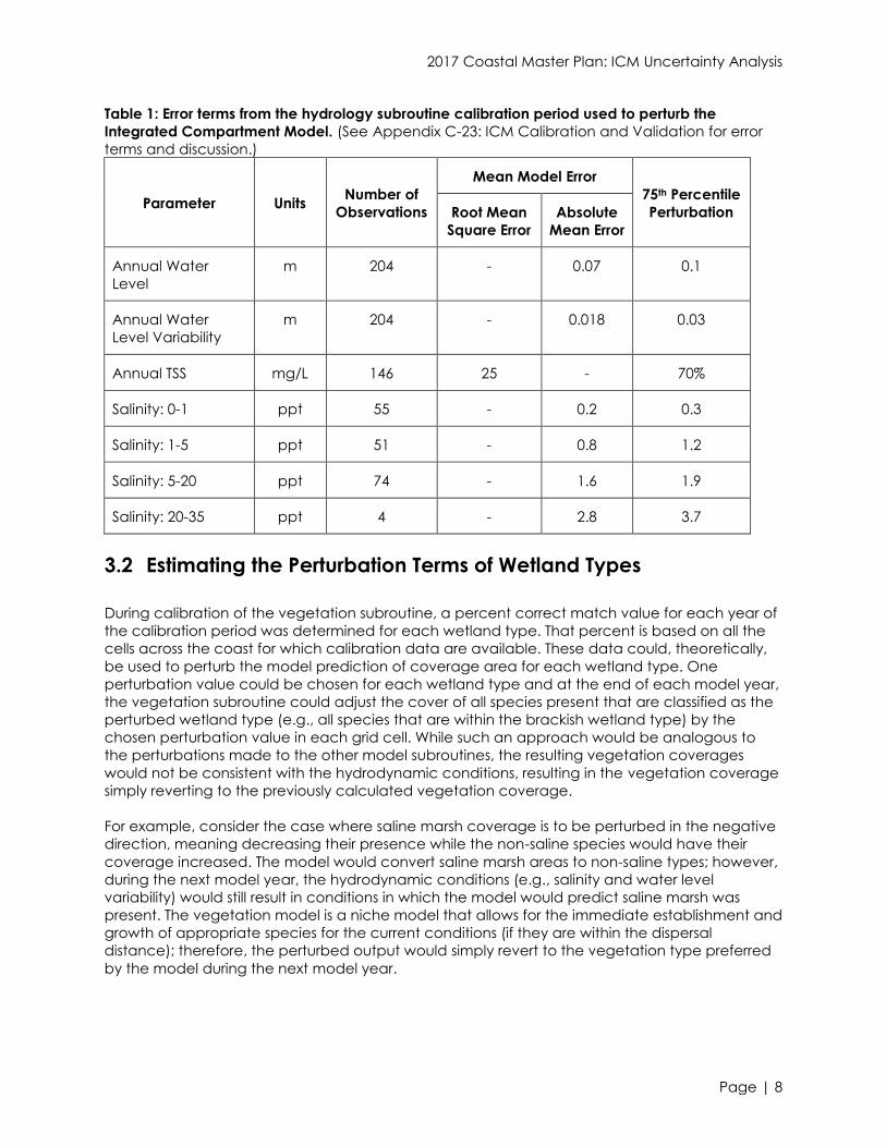
3.1 Estimating the Perturbation Terms for Water Level, Salinity, and
Total Suspended Solids
For annual water level, standard deviation of annual water level, two-week salinity, and TSS, a
distribution of points around the mean was derived based on the statistical analysis performed
during the calibration process. The two-week salinity comparison is a more stringent assessment
on model performance than annual mean salinity (see Section 4.0). Therefore, all salinity
perturbations throughout this analysis were based solely upon the two-week error values. The
mean is the variable value used in the calibrated model, but a probability distribution of the
error around the mean is not fully known; therefore, a normal distribution was assumed and used
to calculate the +/- 25th and +/- 75th percentiles for both the RMSE and the MAE. The UA
considered the composite uncertainty of multiple variables (the list of 10 variables provided
above in Section 2.2). This led to the decision to select the 25th and 75th percentiles instead of a
wider range (e.g., 5th and 95th percentiles). If a wider range is considered, the likelihood of
occurrence of the 5th or 95th percentile of all model variables simultaneously is quite low. The 25th
and 75th percentiles present a more likely space of occurrence.
The difference between the RMSE and MAE and whether one statistical tool is favorable over
the other in terms of average model performance has been argued in literature (e.g., Willmott &
Matsuura, 2005; Chai & Draxler, 2014). Although it is beyond the scope of this document to
contribute to this debate, the MAE assigns a linear score where all individual differences are
weighted equally in the average, while the RMSE gives a relatively high weight to large errors.
For this analysis, the MAE was used to estimate the perturbation values for all variables, with the
exception of TSS, which had a much wider spread in error magnitudes. To account for the wide
range in TSS values, the error was also adjusted as a percentage, rather than as a simple
magnitude. This allowed for regions of the model with higher TSS concentrations to be perturbed
by a value on the same order of magnitude as the predicted values. A similar approach was
used for the salinity perturbations, but rather than a percent error term, the salinity observations
were bracketed into four regimes, ranging from fresh to saline, so that the error in fresh areas
would not unduly result in a lower magnitude of perturbation in the saline regions. Model
performance for salinity was quantified for two different salinity calculations, annual mean
salinity and the two-week mean salinity. Model performance was poorest when comparing the
short-term two-week mean salinity to observed values, as compared to the long term annual
calculations. Therefore, the larger error calculated from the two-week mean salinity was used for
perturbations in this analysis. All salinity values used in the model (either long term salinity for the
vegetation subroutine, or short-term salinity for wetland collapse thresholds in the morphology
subroutine) were perturbed by the same salinity perturbation, which was set equal to the more
conservative (e.g., higher) error estimated by the two-week mean salinity calibration error.
A set of experiments was designed (described in detail in Section 4 below), and the error terms
used in the perturbations are summarized in Table 1.
2017 Coastal Master Plan: ICM Uncertainty Analysis
Page | 8
Table 1: Error terms from the hydrology subroutine calibration period used to perturb the
Integrated Compartment Model. (See Appendix C-23: ICM Calibration and Validation for error
terms and discussion.)
Parameter Units Number of
Observations
Mean Model Error
75th Percentile
Perturbation Root Mean
Square Error
Absolute
Mean Error
Annual Water
Level
m 204 - 0.07 0.1
Annual Water
Level Variability
m 204 - 0.018 0.03
Annual TSS mg/L 146 25 - 70%
Salinity: 0-1 ppt 55 - 0.2 0.3
Salinity: 1-5 ppt 51 - 0.8 1.2
Salinity: 5-20 ppt 74 - 1.6 1.9
Salinity: 20-35 ppt 4 - 2.8 3.7
3.2 Estimating the Perturbation Terms of Wetland Types
During calibration of the vegetation subroutine, a percent correct match value for each year of
the calibration period was determined for each wetland type. That percent is based on all the
cells across the coast for which calibration data are available. These data could, theoretically,
be used to perturb the model prediction of coverage area for each wetland type. One
perturbation value could be chosen for each wetland type and at the end of each model year,
the vegetation subroutine could adjust the cover of all species present that are classified as the
perturbed wetland type (e.g., all species that are within the brackish wetland type) by the
chosen perturbation value in each grid cell. While such an approach would be analogous to
the perturbations made to the other model subroutines, the resulting vegetation coverages
would not be consistent with the hydrodynamic conditions, resulting in the vegetation coverage
simply reverting to the previously calculated vegetation coverage.
For example, consider the case where saline marsh coverage is to be perturbed in the negative
direction, meaning decreasing their presence while the non-saline species would have their
coverage increased. The model would convert saline marsh areas to non-saline types; however,
during the next model year, the hydrodynamic conditions (e.g., salinity and water level
variability) would still result in conditions in which the model would predict saline marsh was
present. The vegetation model is a niche model that allows for the immediate establishment and
growth of appropriate species for the current conditions (if they are within the dispersal
distance); therefore, the perturbed output would simply revert to the vegetation type preferred
by the model during the next model year.

2017 Coastal Master Plan: ICM Uncertainty Analysis
Page | 9
The initial intent of this analysis was to determine the uncertainty associated with each model
subroutine. However, the perturbation of the vegetation output would not be sustained unless
the hydrodynamic model outputs are concurrently perturbed. In essence, perturbing the
hydrodynamic model is sufficient to provide an idea about the impact and variability to the
vegetation output. Specifically, the two primary drivers of the vegetation model, salinity and
water level variability, were already included in this analysis. As will be shown in a later section,
the perturbations of these two variables do not have a particularly large impact on the modeled
coast wide land area, but they do result in different vegetation patterns. This provides an indirect
approach to assess the impact of uncertain vegetation coverage on predicted land loss in the
model. Therefore, the vegetation model output was not perturbed as part of this analysis.
3.3 Estimating the Perturbation Terms for Organic Loading
The accretion calculation within the morphology subroutine is derived from two sources: 1) the
inorganic sediment load predicted by the hydrology subroutine and 2) the OM and BD values
assigned to each marsh type (this is spatially varied across the coast). As discussed above, the
uncertainty in the mineral depositional rates was perturbed based on the hydrology subroutine’s
TSS calibration statistics. The uncertainty in the organic component is not easily quantified from
the measured Cesium cores used in the calibration of the subroutine. Therefore, in the UA, the
organic portion of the accretion calculation was perturbed based on the variability of the
measured OM and BD data used as model input. The organic accretion is directly proportional
to the OM and BD values used; therefore, an analysis of the variability in these data results in a
quantifiable range in the organic component of the vertical accretion rates.
The underlying dataset used to derive the OM and BD input data included not only mean
values, but also standard deviations. The 25th and 75th percentiles of OM and BD input values
were used to examine the uncertainty of the organic component of accretion calculations. The
low BD values were paired with the high OM values to result in the maximum increase in vertical
accretion calculations, and vice versa for the maximum decrease in accretion. The underlying
dataset was summarized by basin and marsh type, which is the format that the model applies
these organic loading rates, and therefore perturbation values vary spatially.
4.0 Experimental Design and Results – Phase 1
In the first set of experiments, only one variable was perturbed at a time. Table 2 shows the list of
experiments performed. The first four experiments focused on perturbing the two-week salinity.
Four perturbations were considered corresponding to +/- 25th and +/- 75th percentiles of the MAE
distribution around the mean. Change in coastal land loss across the entire model domain, as
compared against the “baseline” FWOA model run, is described below. Figures 2 and 3 show a
very small change in total land area associated with +/- 25th perturbations (runs U01 and U02).
Based on the outcome of the first four experiments, only +/- 75th percentiles of the MAE
distribution were considered for the remainder of the variables. Also based on the outcome of
these four experiments, a separate perturbation for the annual salinity was not performed;
instead, the two-week salinity perturbation was used and applied to all salinity output (used in
both the vegetation and morphology subroutines). If a separate annual perturbation was
calculated, it would have been smaller than the two-week perturbation that was already
tested. Clearly that would have resulted in less deviation from the “baseline” model run than
what has been observed from the two-week salinity perturbations shown through the first four
experiments. In addition to the first four experiments, eight experiments (two perturbations for
2017 Coastal Master Plan: ICM Uncertainty Analysis
Page | 10
each of the four remaining variables) were performed. The perturbation values are summarized
in Table 2.
In all 12 experiments, one variable was perturbed at a time. The response of the model to these
perturbations was analyzed through the total land area (across the entire coast) and land area
in each ecoregion (spatial units identified within the ICM). The analysis also shows the behavior
of the model response over 50 years, as the model output could potentially diverge from the
“baseline” model run over time.
Table 2: Experimental runs – variables and individual perturbations.
Model Run Perturbed Variable Perturbation Magnitude
U01 Salinity + 25th percentile
U02 Salinity - 25th percentile
U03 Salinity + 75th percentile
U04 Salinity - 75th percentile
U05 Annual water level (m) + 75th percentile
U06 Annual water level (m) - 75th percentile
U07 Annual water level variability (m) + 75th percentile
U08 Annual water level variability (m) - 75th percentile
U09 Annual TSS (mg/l) + 75th percentile
U10 Annual TSS (mg/l) - 75th percentile
U11 Organic sediment More accretion (increased OM and
decreased BD)
U12 Organic sediment Less accretion (decreased OM and
increased BD)
2017 Coastal Master Plan: ICM Uncertainty Analysis
Page | 11
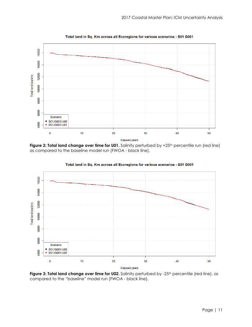
Figure 2: Total land change over time for U01. Salinity perturbed by +25th percentile run (red line)
as compared to the baseline model run (FWOA - black line).
Figure 3: Total land change over time for U02. Salinity perturbed by -25th percentile (red line), as
compared to the “baseline” model run (FWOA - black line).
2017 Coastal Master Plan: ICM Uncertainty Analysis
Page | 12
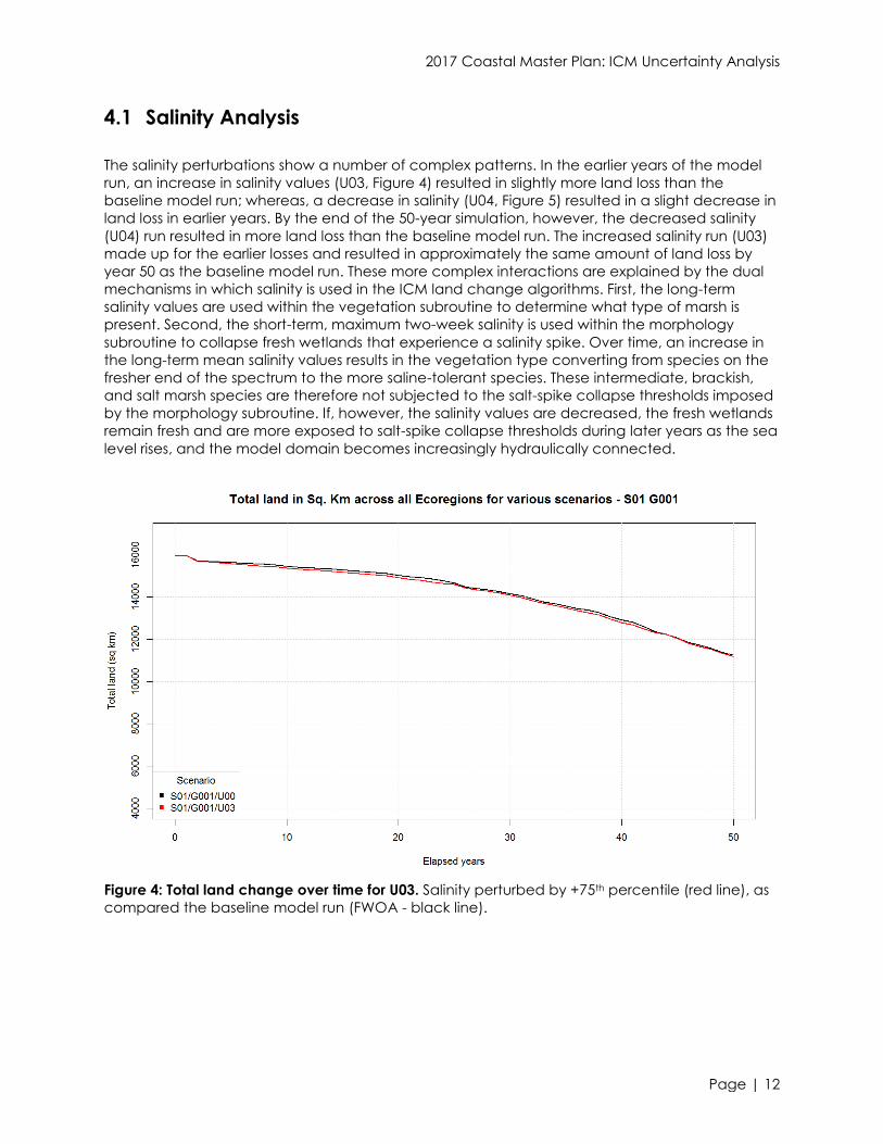
4.1 Salinity Analysis
The salinity perturbations show a number of complex patterns. In the earlier years of the model
run, an increase in salinity values (U03, Figure 4) resulted in slightly more land loss than the
baseline model run; whereas, a decrease in salinity (U04, Figure 5) resulted in a slight decrease in
land loss in earlier years. By the end of the 50-year simulation, however, the decreased salinity
(U04) run resulted in more land loss than the baseline model run. The increased salinity run (U03)
made up for the earlier losses and resulted in approximately the same amount of land loss by
year 50 as the baseline model run. These more complex interactions are explained by the dual
mechanisms in which salinity is used in the ICM land change algorithms. First, the long-term
salinity values are used within the vegetation subroutine to determine what type of marsh is
present. Second, the short-term, maximum two-week salinity is used within the morphology
subroutine to collapse fresh wetlands that experience a salinity spike. Over time, an increase in
the long-term mean salinity values results in the vegetation type converting from species on the
fresher end of the spectrum to the more saline-tolerant species. These intermediate, brackish,
and salt marsh species are therefore not subjected to the salt-spike collapse thresholds imposed
by the morphology subroutine. If, however, the salinity values are decreased, the fresh wetlands
remain fresh and are more exposed to salt-spike collapse thresholds during later years as the sea
level rises, and the model domain becomes increasingly hydraulically connected.
Figure 4: Total land change over time for U03. Salinity perturbed by +75th percentile (red line), as
compared the baseline model run (FWOA - black line).

2017 Coastal Master Plan: ICM Uncertainty Analysis
Page | 13
Figure 5: Total land change over time for U04. Salinity perturbed by -75th percentile (red line), as
compared to the baseline model run (FWOA - black line).
4.2 Water Level Analysis
The mean water level perturbations, U05 and U06, resulted in the largest divergence from the
baseline model run (Figures 6 and 7). The coast wide land loss divergence followed an intuitive
response given that inundation is a key land loss mechanism in the ICM. The +75th percentile
perturbation (U05), which perturbed the water level estimates upward, resulted in more land loss
over time, whereas lowering the water level estimates using the -75th percentile perturbation
(U06) maintained more land over the 50 year simulation. These results are consistent with those
from the future scenarios analysis that indicate that coastal land area, as predicted by the ICM,
is sensitive to varying rates of sea level rise (Appendix C: Chapter 2).
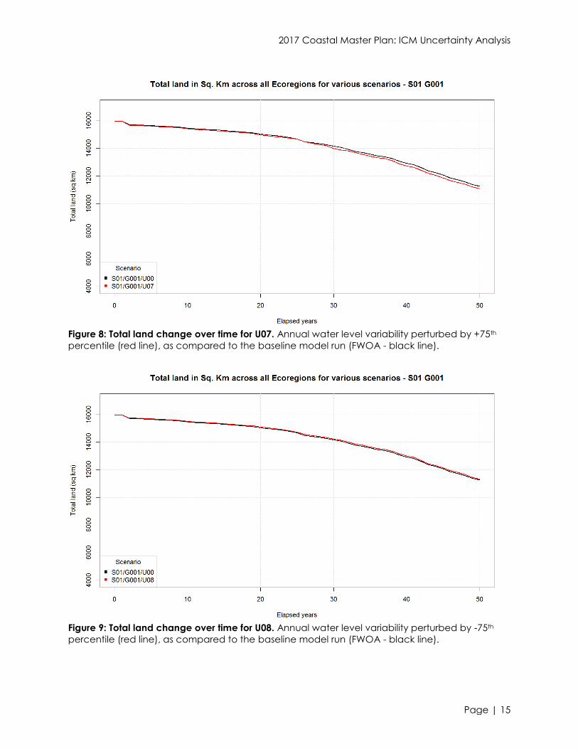
Increasing water level variability (run U07) resulted in slightly more land loss over time, but
decreasing this parameter (run U08) did not have a large impact on the coast wide land loss
calculations (Figures 8 and 9). The relatively minimal impact of these perturbations, on land area,
is likely due to the small magnitude of the water level variability error term (+/- 0.03 meters at 75th
percentile). This variable is only used within the vegetation subroutine and is on the same order
of magnitude as the resolution of the vegetation subroutine input data. The probability of
establishment and mortality of the individual vegetation species is provided in increments of 0.04
meters of water level variability. Therefore, perturbing the model output by the 75th percentile of
the error is resulting in a very small adjustment to the establishment/mortality probabilities within
the vegetation subroutine. These perturbations impacted the relative extent of specific
vegetation types by the end of the model run (Figure 10 – vegetation at year 50); however, the
magnitude of these changes in cover type did not substantially impact the coast wide area of
land loss. While these perturbations did have some impact on vegetation type, and
subsequently the collapse mechanisms driving land loss, the magnitude of these impacts were
overwhelmed, at the coast wide scale, by other drivers of land loss throughout the 50-year
simulation. In other words, the change in water level variability may change the vegetation type

2017 Coastal Master Plan: ICM Uncertainty Analysis
Page | 14
in the model, but the relatively minor differences in collapse mechanism between vegetation
types was overwhelmed by the relative sea level rise throughout the model run.
Figure 6: Total land change over time for U05. Annual water level perturbed by +75th percentile
(red line), as compared to the baseline model run (FWOA - black line).
Figure 7: Total land change over time for U06. Annual water level perturbed by -75th percentile
(red line), as compared to the baseline model run (FWOA - black line).
2017 Coastal Master Plan: ICM Uncertainty Analysis
Page | 15
Figure 8: Total land change over time for U07. Annual water level variability perturbed by +75th
percentile (red line), as compared to the baseline model run (FWOA - black line).
Figure 9: Total land change over time for U08. Annual water level variability perturbed by -75th
percentile (red line), as compared to the baseline model run (FWOA - black line).

2017 Coastal Master Plan: ICM Uncertainty Analysis
Page | 16
Figure 10: Relative abundance of vegetation types over the 50-year simulation; FWOA and U07 (+75th percentile of annual water level
variability).

2017 Coastal Master Plan: ICM Uncertainty Analysis
Page | 17
4.3 Total Suspended Solids Analysis
The coast wide land loss predictions appeared to be insensitive to perturbations to the annual
inorganic TSS concentration that was perturbed in runs U09 and U10 (Figures 11 and 12). This can
be explained by a number of factors. First, the TSS perturbation value (38 mg/L) was determined
from the calibration error of a fairly small dataset. Both the observed and modeled TSS data
varied by as much as an order of magnitude, and it is likely that the model area that would be
most sensitive to a change in land area due to TSS perturbations would be the areas of the
largest TSS concentrations. These areas are on the extremes of the TSS distribution and are
therefore likely insensitive to just a +/- 75th percentile perturbation. Second, land gain in the
model domain and in the real landscape (e.g., Wax Lake Delta) is occurring where there is a
steady sediment supply from outside the system. The entrainment of estuarine bed sediments is
not a large driver of land gain in coastal Louisiana (Burkett et al., 2007). Therefore, the inflow TSS
boundary conditions are likely a much more sensitive parameter than the calculated TSS values
from the deposition/resuspension routines in the hydrology subroutine. Third, the areas in the
FWOA model run that experience land gain are limited. Overall, the impact of the TSS
perturbations at the coast wide or ecoregion scales originates primarily from specific locations
with definitive external sediment loading (e.g., Wax Lake Delta, West Bay, Big Mar, etc.) and
ultimately did not result in significant response to the perturbations. It should be noted that the
TSS perturbations might be important for certain project types such as large sediment diversions.
Figure 11: Total land change over time for U09. Annual inorganic TSS perturbed by +75th
percentile (red line), as compared to the baseline model run (FWOA - black line).

2017 Coastal Master Plan: ICM Uncertainty Analysis
Page | 18
Figure 12: Total land change over time for U10. Annual inorganic TSS perturbed by -75th
percentile (red line), as compared to the baseline model run (FWOA - black line).
4.4 Organic Sediment Analysis
Perturbing the organic accretion, as determined by OM input and BD values, resulted in an
intuitive model response. Higher accretion due to high OM and low BD (run U11) resulted in a
substantial increase in coast wide land area at year 50, as compared to the baseline model run
(Figure 13). Conversely, run U12, which modeled lower accretion rates, resulted in a decrease in
land area at year 50 (Figure 14). The impact of these perturbations on coast wide land area at
year 50 is similar in magnitude to the mean water level perturbations (runs U05 and U06).
However, the organic sediment perturbations are asymmetric around the baseline run. This
asymmetry could be explained by areas of collapsed land in the baseline run that are close to
but slightly above the collapse threshold in the baseline run. Once an area has collapsed, it will
not be influenced by a decrease OM/BD; it simply remains collapsed. However, an increase to
the OM/BD would sustain an area that was just on the threshold of collapsing/not collapsing, hence the asymmetry in the results.

2017 Coastal Master Plan: ICM Uncertainty Analysis
Page | 19
Figure 13: Total land change over time for U11. Organic sediment perturbed to increase
accretion by increasing organic matter content and reducing bulk density values (red line), as
compared to the baseline model run (FWOA - black line).
Figure 14: Total land change over time for U12. Organic sediment perturbed to decrease
accretion by decreasing organic matter content and increasing bulk density values (red line), as
compared to the baseline model run (FWOA - black line).
2017 Coastal Master Plan: ICM Uncertainty Analysis
Page | 20
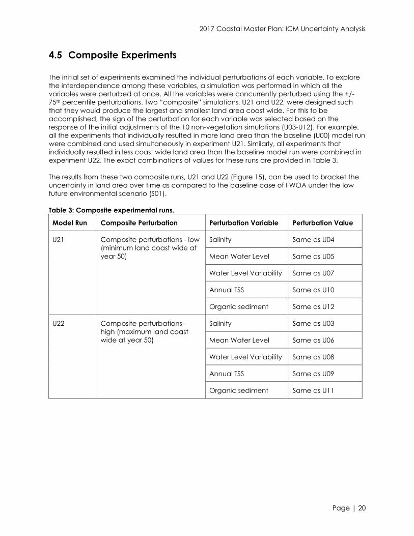
4.5 Composite Experiments
The initial set of experiments examined the individual perturbations of each variable. To explore
the interdependence among these variables, a simulation was performed in which all the
variables were perturbed at once. All the variables were concurrently perturbed using the +/-
75th percentile perturbations. Two “composite” simulations, U21 and U22, were designed such
that they would produce the largest and smallest land area coast wide. For this to be
accomplished, the sign of the perturbation for each variable was selected based on the
response of the initial adjustments of the 10 non-vegetation simulations (U03-U12). For example,
all the experiments that individually resulted in more land area than the baseline (U00) model run
were combined and used simultaneously in experiment U21. Similarly, all experiments that
individually resulted in less coast wide land area than the baseline model run were combined in
experiment U22. The exact combinations of values for these runs are provided in Table 3.
The results from these two composite runs, U21 and U22 (Figure 15), can be used to bracket the
uncertainty in land area over time as compared to the baseline case of FWOA under the low
future environmental scenario (S01).
Table 3: Composite experimental runs.
Model Run Composite Perturbation Perturbation Variable Perturbation Value
U21 Composite perturbations - low
(minimum land coast wide at
year 50)
Salinity Same as U04
Mean Water Level Same as U05
Water Level Variability Same as U07
Annual TSS Same as U10
Organic sediment Same as U12
U22 Composite perturbations -
high (maximum land coast
wide at year 50)
Salinity Same as U03
Mean Water Level Same as U06
Water Level Variability Same as U08
Annual TSS Same as U09
Organic sediment Same as U11
2017 Coastal Master Plan: ICM Uncertainty Analysis
Page | 21
Figure 15: Total land change over time for U21 (green line) and U22 (red line). The composite
uncertainty runs provide the upper and lower limits on model uncertainty, as compared to the
baseline model run (FWOA - black line).
5.0 Spatial Analysis of Uncertainty – Phase 1
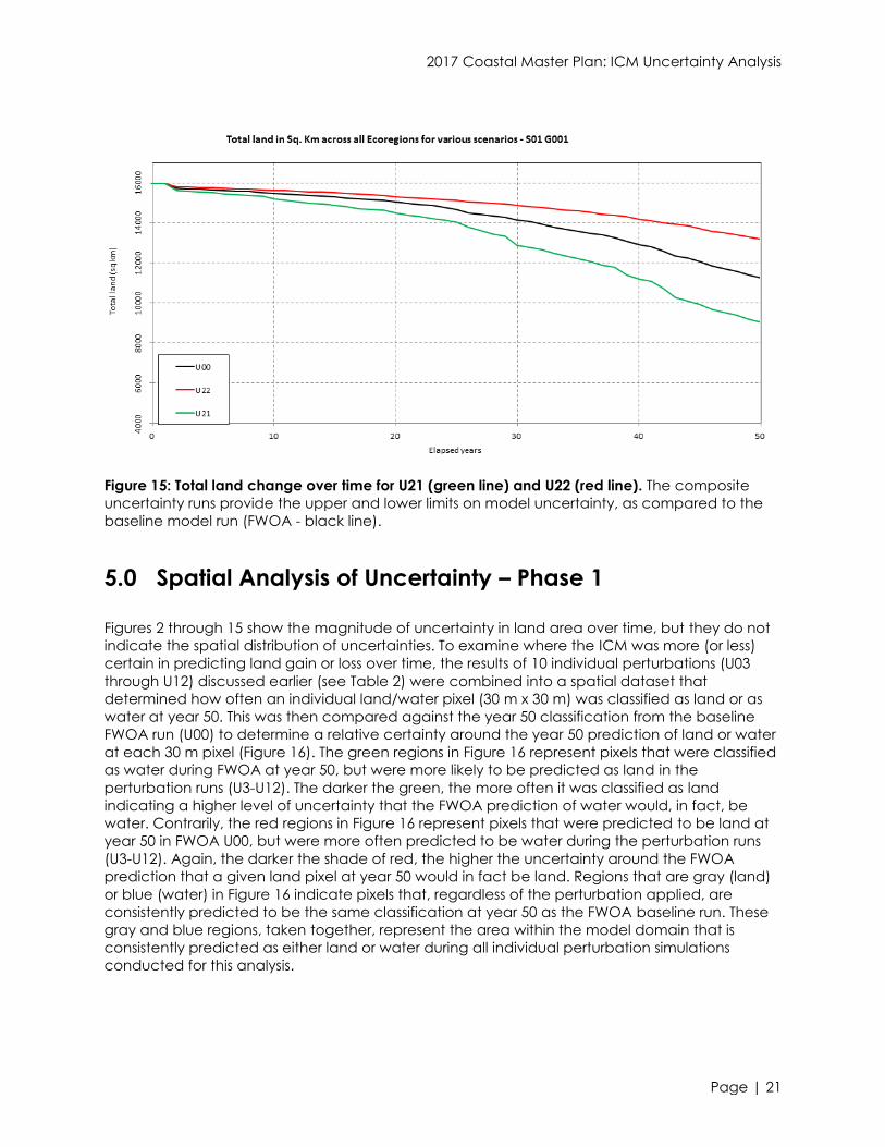
Figures 2 through 15 show the magnitude of uncertainty in land area over time, but they do not
indicate the spatial distribution of uncertainties. To examine where the ICM was more (or less)
certain in predicting land gain or loss over time, the results of 10 individual perturbations (U03
through U12) discussed earlier (see Table 2) were combined into a spatial dataset that
determined how often an individual land/water pixel (30 m x 30 m) was classified as land or as
water at year 50. This was then compared against the year 50 classification from the baseline
FWOA run (U00) to determine a relative certainty around the year 50 prediction of land or water
at each 30 m pixel (Figure 16). The green regions in Figure 16 represent pixels that were classified
as water during FWOA at year 50, but were more likely to be predicted as land in the
perturbation runs (U3-U12). The darker the green, the more often it was classified as land
indicating a higher level of uncertainty that the FWOA prediction of water would, in fact, be
water. Contrarily, the red regions in Figure 16 represent pixels that were predicted to be land at
year 50 in FWOA U00, but were more often predicted to be water during the perturbation runs
(U3-U12). Again, the darker the shade of red, the higher the uncertainty around the FWOA
prediction that a given land pixel at year 50 would in fact be land. Regions that are gray (land)
or blue (water) in Figure 16 indicate pixels that, regardless of the perturbation applied, are
consistently predicted to be the same classification at year 50 as the FWOA baseline run. These
gray and blue regions, taken together, represent the area within the model domain that is
consistently predicted as either land or water during all individual perturbation simulations
conducted for this analysis.

2017 Coastal Master Plan: ICM Uncertainty Analysis
Page | 22
Figure 16: Land/water prediction uncertainty – all individual perturbations at year 50.
The regions where the perturbed runs consistently result in a year 50 land/water value different
than the FWOA U00 case (dark green and dark red) indicate that there are many land/water
pixels that are consistently impacted by perturbations. These are the pixels that are close to a
collapse threshold in the baseline run (U00). Once perturbed, it is quite likely for these pixels to
result in a different outcome at year 50, regardless of the perturbation applied. The regions that
are seldom different from the baseline (light green and light red), on the other hand, indicate
pixels that respond to one (or two) very specific perturbations only. Based upon the magnitude
of impact from the individual runs, it is likely that these pixels of lower uncertainty are ‘activated’
into losing or sustaining land when the mean water level or the organic accretion perturbations
are applied. Physically, these are the only two perturbed variables that will directly influence the
elevation and could result in these changes.
A composite run in which the mean water level and the organic accretion are perturbed in
opposite directions (e.g., lower mean water level, higher organic accretion, and vice versa), will
potentially have a synergistic effect on land pixels that are lost or sustained. Figure 17 shows that
this synergistic effect does indeed take place when the variables are perturbed simultaneously.
The purple regions in Figure 17 are pixels that are land at year 50 from the composite run, U22,
that were water in all individual perturbation runs as well as the FWOA baseline.
Some of the land/water pixels that did not change from their baseline condition during the
individual perturbations did respond to the composite runs of U21 and U22. Thus, a complete set
of composite perturbations needed to be analyzed to determine if U21 and U22 bracket the
uncertainty in coastal land area over time.

2017 Coastal Master Plan: ICM Uncertainty Analysis
Page | 23
Figure 17: Land/water prediction uncertainty – all individual perturbations and composite run U22
(near Myrtle Grove, year 50).
From the individual perturbation runs (U09 and U10), it was determined that errors in suspended
inorganic sediments (TSS) did not result in any appreciable change in coast wide land area over
time. Removing TSS from further analysis allowed for 16 additional simulations that would test
model uncertainty as a function of all possible permutations of two perturbed values for mean
water level, salinity, water level variability, and organic accretion. These 16 permutations (Table
4) were analyzed, allowing for a thorough determination of uncertainty in the FWOA land/water
predictions and the relative sensitivity to the different perturbation permutations.
Table 4: Experimental runs – composite perturbations – all permutations.
Model Run Salinity Mean Water Level Water Level Variability Organic Sediment
U25 +75 percentile +75 percentile +75 percentile +OM/-BD
U26 +75 percentile +75 percentile +75 percentile -OM/+BD
U27 +75 percentile +75 percentile -75 percentile +OM/-BD
U28 +75 percentile +75 percentile -75 percentile -OM/+BD
U29 +75 percentile -75 percentile +75 percentile +OM/-BD
U30 +75 percentile -75 percentile +75 percentile -OM/+BD

2017 Coastal Master Plan: ICM Uncertainty Analysis
Page | 24
Model Run Salinity Mean Water Level Water Level Variability Organic Sediment
U31 +75 percentile -75 percentile -75 percentile +OM/-BD
U32 +75 percentile -75 percentile -75 percentile -OM/+BD
U33 -75 percentile +75 percentile +75 percentile +OM/-BD
U34 -75 percentile +75 percentile +75 percentile -OM/+BD
U35 -75 percentile +75 percentile -75 percentile +OM/-BD
U36 -75 percentile +75 percentile -75 percentile -OM/+BD
U37 -75 percentile -75 percentile +75 percentile +OM/-BD
U38 -75 percentile -75 percentile +75 percentile -OM/+BD
U39 -75 percentile -75 percentile -75 percentile +OM/-BD
U40 -75 percentile -75 percentile -75 percentile -OM/+BD
After completion of these 16 permutations, the output from U31 was compared to U22. The only
difference between these two composite perturbation runs was the inclusion of TSS perturbation
in U22; all other perturbed variables were identical between U22 and U31. As Figure 18 shows,
there was some impact at very small scales (e.g., near Davis Pond); however, at a coast wide
scale, there were only negligible differences between these two composite perturbations.
Therefore, the inclusion of TSS perturbations was determined to be unnecessary in assessing
overall model uncertainty.

2017 Coastal Master Plan: ICM Uncertainty Analysis
Page | 25
Figure 18: Land/water prediction uncertainty – composite perturbations with (U22) and without
perturbed TSS (U31); near Davis Pond, year 50.
As predicted by analyzing the pixels affected by the composite run U22, but none of the
individual perturbations (Figure 17), the range in land area change over time is highly sensitive to
perturbations to mean water level and organic accretion. In Figure 19, the four runs that result in
the highest land area over time (U29, U31, U37, and U39) all included a decrease in mean water
level and an increase in organic accretion. The salinity and water level variability perturbations
appear to drive a difference in vegetation cover, though if the mean water level and organic
accretion perturbation counteract one another, the salinity and water level variability
perturbations do appear to have some impact on the final land area. However, regardless of
the exact combination, all of these runs appear to result in slightly more land at year 50 than the
baseline U00 run.
If the mean water level is increased at the same time as the organic accretion is decreased
(U26, U28, U34, and U36), it does not appear as if the exact combination of salinity and water
level variability makes much of an impact. The final land area in the last decade of these model
runs is remarkably consistent, indicating more loss coast wide than the U00 FWOA baseline run.

2017 Coastal Master Plan: ICM Uncertainty Analysis
Page | 26
Figure 19: Baseline FWOA land area over time (U00, black line) compared against all 16
permutations of composite uncertainty perturbations.
6.0 Assessing Future Without Action Model Uncertainty
Under the High Environmental Scenario – Phase 2
6.1 Methodology for Assessing Spatial Patterns of Uncertainty –
Phase 2
In addition to the temporal and spatial assessment of overall parametric uncertainty, the outputs
from the FWOA analysis provided in the previous sections helped to identify the key model
variables with significant impact on land area and to examine sensitivity to change of the
perturbation terms for each variable. This examination was then used to design a streamlined UA
for application under a more severe future scenario, as well as the uncertainty in land
predictions of the implemented 2017 Draft Coastal Master Plan. Based on the results previously
presented, it appears that the interdependency among the model variables is important (Figure
19). Therefore, the 16 permutations presented in Table 4 and Figure 19 were applied to the two
high scenario FWOA analyses (i.e., from version 1 and version 3 of the ICM) and the high
scenario 2017 Draft Coastal Master Plan analysis conducted in the second phase of the UA.

2017 Coastal Master Plan: ICM Uncertainty Analysis
Page | 27
The overall spatial patterns of model uncertainty across the coast from each of the four cases
(i.e., the three high scenario simulations just discussed and the low scenario FWOA from ICM
version 1) are shown in Figure 20 through Figure 23. For visualization purposes, each land/water
pixel was classified with a relative sense of uncertainty. This relative uncertainty was determined
for each set of 16 permutations. The more often a permutation resulted in a land/water pixel
having a different outcome at year 50 than the baseline (U00) case, the higher the relative
uncertainty for that pixel. If a land/water pixel was predicted to be different than the baseline
case in 6% or less of the permutations (e.g., no more than one of the 16 permutations resulted in
a different outcome at year 50) that land/water pixel was classified as being either certain land
or certain water. A land/water pixel that returned a year 50 result that differed from the baseline
in 6-37% of the permutations (two to six of the 16 permutations) was considered to have a low
possibility of having a different outcome compared to the baseline run. Differences from
baseline in 38-69% of the permutations indicated a medium possibility of a different outcome
than baseline, and any pixel that was different from the baseline in more than 69% of the
permutations was classified as having a high possibility of having a year 50 value that differed
from the baseline run.
Hypothetically, if the following maps were solid red, this would indicate that all land predicted to
be remaining at year 50 was in fact uncertain and all permutations resulted in a prediction of
less land at year 50 than the baseline. If the maps were solid green, this would indicate that all
areas predicted to be water at year 50 would in fact be predicted as land under all other non-
baseline cases. As Figure 20 through Figure 23 show, the patterns are mixed and vary between
both the environmental scenarios and the FWOA or Draft 2017 Coastal Master Plan conditions
that are modeled. In simple terms, more red on the map implies that the model overestimates
land area, and more green implies that the model underestimates land area.
6.2 Comparison Between Low and High Scenarios
The impact upon model uncertainty between the low and high scenarios is shown by
comparing the low and high scenario analyses that were conducted using ICM_v1 (S01 G001
and S03 G001, respectively). The similarities and differences in spatial variability of these relative
uncertainties are evident in Figure 20 and Figure 21. The portion of the model domain west of
Vermilion Bay appears to be a region of variable uncertainty under the low scenario (Figure 20);
a relatively large portion of this area is sensitive to differing outcomes under the 16 permutations.
Either regions of baseline-predicted land are repeatedly predicted as water under the
uncertainty permutations (red pixels) or baseline-predicted water repeatedly is predicted to be
land under the permutations (green pixels). This indicates a region of the model that is (more or
less) symmetric around the baseline run; which is also evident in the time series of land area
predicted under all permutations in the western region (see Figure 34 through Figure 37 for
ecoregions west of the Atchafalaya Basin). Under the high scenario (Figure 21), however, large
portions of the domain are not as varied at year 50 across the 16 permutations as they were
under the low scenario. Much of the area that is consistently predicted under the high scenario
is due to that fact that much more area is predicted to be water at year 50 under the high
scenario in the baseline run and in each permutation. While there are some regions of baseline-
predicted water that have a low possibility of being predicted land under the permutations,
some visually prominent features are: the baseline-predicted area of land along the Gulf
shoreline south of Vermilion Bay, Grand Lake, and White Lake that has a high possibility of being
water under the permutations and the variable uncertainty of the Maurepas swamp area under
the low scenario that is much less uncertain under the high scenario. These changes in
uncertainty are largely the result of how the ICM_v1 algorithm treats bare ground that is not

2017 Coastal Master Plan: ICM Uncertainty Analysis
Page | 28
suitable for any modeled vegetated and the salinity predictions of ICM_v1. Version 3 of the ICM
(ICM_v3) addressed these issues and is detailed in the following section.
Figure 20: Relative uncertainty in baseline FWOA predictions under the low scenario using
version 1 of the ICM (S01 G001).

2017 Coastal Master Plan: ICM Uncertainty Analysis
Page | 29
Figure 21: Relative uncertainty in baseline FWOA predictions under the high scenario using
version 1 of the ICM (S03 G001).
6.3 Comparison Between ICM Versions 1 and 3
Upon the completion of the project-level runs for the 2017 Coastal Master Plan analysis, several
adjustments were made to the ICM code to address various model instabilities and unrealistic
model behaviors under a few select conditions. The two main changes that impacted the
model uncertainty results were a recalibration of salinity transfer in some of the large model
compartments in the fresh upstream regions and a change that allowed for areas of persistent
bare ground (where conditions are not suitable for any modeled vegetation species to be
present) to collapse into open water if repeatedly inundated by the annual mean water level.
These changes are discussed in detail in Attachment C3-22: Integrated Compartment Model
(ICM) Development and Attachment C3-23: ICM Calibration, Validation, and Performance
Assessment.
The ability of inundated bare ground to collapse into open water impacts the uncertainty
analysis results in three particular areas of the model domain. First, the Gulf shoreline south of
Vermilion Bay, Grand Lake, and White Lake are modeled as baseline-predicted land in ICM_v1;
however, they have a relatively high possibility of being water under the permutations (Figure
21). Once the bare ground is allowed to collapse in ICM_v3, these ridges are persistently
predicted to be water at year 50 (Figure 22); a change from high uncertainty in ICM_v1 to low
uncertainty in ICM_v3. The other two areas impacted by the bare ground collapse change are
in Upper Barataria in the vicinity of Lake Bouef and in Breton Sound. Again, in ICM_v1, these
regions were persistently predicted to be bare ground in the last few model years (due to a rise
in salinities beyond the tolerance range of any nearby vegetation species) and were
subsequently predicted to be land at year 50 in nearly all permutations (Figure 21). Under

2017 Coastal Master Plan: ICM Uncertainty Analysis
Page | 30
ICM_v3, these areas were subjected to collapse if persistently non-vegetated; this resulted in
these areas of baseline-predicted land now with a high possibility of being water (Figure 22).
Figure 22: Relative uncertainty in baseline FWOA predictions under the high scenario using
version 3 of the ICM (S03 G300).
The change to salinity calculations made between ICM_v1 and ICM_v3 had a more subtle
effect on the spatial patterns of model uncertainty, with almost all differences occurring in the
Upper Pontchartrain ecoregion (upstream of Lake Maurepas) and in the Upper Barataria
ecoregion (upstream and around Lac des Allemandes). The changes in the Maurepas region
are primarily due to areas that were predicted to be water at year 50 under nearly all ICM_v1
permutations (white or light green pixels south of I-10 in Figure 21), but were predicted to be land
with a low to medium possibility of being water under the ICM_v3 permutations (pink or red
pixels south of I-10 in Figure 22). The Upper Barataria region had a much clearer response to the
ICM_v3 changes. The improved representation of salinity in this region under ICM_v3 resulted in a
more consistent response than under ICM_v1, with a low to medium possibility that the baseline-
predicted land in this region would be water under the uncertainty permutations. The changes
made to salinity calculations between ICM_v1 and ICM_v3 resulted in more stable salinity
calculations in these upstream areas, which in turn resulted in fewer salinity spike events in
ICM_v3. Under ICM-v1, the relatively unstable salinity calculations resulted in a greater number of
perturbations resulting in loss of fresh wetland area due to salinity-induced collapse. The unstable
salinity spiking issues of ICM_v1, therefore were more certain than ICM_v3, yet unrealistically
resulting in land loss. The update made to ICM_v3, therefore returned more realistic and stable
salinity results in upstream basins but more variability in land/water predictions at year 50.

2017 Coastal Master Plan: ICM Uncertainty Analysis
Page | 31
7.0 Assessing Model Uncertainty Under the Future With
Action Draft Master Plan
7.1 Spatial Patterns of Future With Draft Master Plan Uncertainty
The 16 uncertainty permutations were also performed for the Draft 2017 Coastal Master Plan
under the high scenario (S03 G400). In the region of the model domain west of the Atchafalaya
Basin, there were a few distinct differences in spatial patterns of uncertainty as compared to the
high scenario FWOA using ICM_v3 (S03 G300) (Figure 23). Namely, there are large areas under
the Future With Draft Master Plan that are predicted to be land under all (or all but one)
permutations. These large, irregular, gray-colored polygons (e.g., around Calcasieu Lake and on
Marsh Island) are in fact the location of numerous marsh creation projects that are implemented
in the western region in the Draft 2017 Coastal Master Plan. These permutations indicate that, as
implemented in the Draft 2017 Coastal Master Plan, these projects will perform consistently
across the uncertainty permutations. In addition to the numerous marsh creation projects in the
western region that are consistently predicted to be land at year 50, east of Calcasieu Lake,
outside of any direct project footprint, there is an increase in the amount of baseline-predicted
water area that has a low to medium possibility of being land.
Like the FWOA uncertainty, an expanse of baseline-predicted water in Central and Western
Terrebonne appears to have a low to medium possibility of being land. However, the Draft 2017
Coastal Master Plan includes diversion projects off the Atchafalaya River that maintain land in
this region; the FWOA baseline-predicted water with low possibility of being land in Central
Terrebonne south of Amelia (Figure 22) becomes baseline-predicted land with a low possibility of
being water under the Draft 2017 Coastal Master Plan (Figure 23). Additional changes in this
central region include several large areas of marsh creation projects. Some of these marsh
creation projects are predicted to be land under nearly all permutations, while others are
baseline-predicted land at year 50 with some possibility of being water under specific
uncertainty permutations. A large marsh creation project further east at the border between
Terrebonne and Barataria ecoregions demonstrates the same trend of being baseline-predicted
land with a low to medium possibility of being water at year 50 under the Draft 2017 Coastal
Master Plan.

2017 Coastal Master Plan: ICM Uncertainty Analysis
Page | 32
Figure 23: Relative uncertainty in baseline Future With Draft Master Plan predictions under the
high scenario using version 3 of the ICM (S03 G400).
Elsewhere in the eastern region of the model domain, the starkest difference between the Draft
2017 Coastal Master Plan and the FWOA are in the upper portions of the Barataria and
Pontchartrain basins. Almost all baseline-predicted land in Upper Barataria north of Highway 90 is
land in nearly all uncertainty permutations. The same behavior is seen upstream of Lake
Maurepas, nearly all baseline-predicted land remains land under all permutations. Both regions
were relatively uncertain under the FWOA (Figure 23); this change in behavior is largely due to
the presence of freshwater diversions into the Maurepas swamp area as well as the presence of
the Lake Pontchartrain Barrier (001.HP.08) hurricane protection project (see Section 5.3.2.3 in
Chapter 4). There is some uncertainty regarding the baseline-predicted land in the Maurepas
landbridge area under the Draft 2017 Coastal Master Plan; however, this was predicted to be
water with a low possibility of being land under the FWOA.
Uncertainty in the areas impacted by Mississippi River diversions varies; immediately adjacent to
the outfalls of both Mid-Barataria and Mid-Breton Diversions, the land built or sustained by the
diversion is maintained under all permutations. In Breton, there is a section of baseline-predicted
water near, but not immediately adjacent to the outfall, that has a high possibility of being land
under the uncertainty permutations. Areas of sustained land further afield in Breton are baseline-
predicted land under the Draft 2017 Coastal Master Plan with a low to medium possibility of
being water. A portion of the most Gulf-ward fringe marsh areas in Breton Sound are predicted
to be water under the baseline Draft 2017 Coastal Master Plan; however, they have a low
possibility of being land under certain permutations. This complex behavior in Breton Sound is
evident in the time series plots of land area over time shown in Figure 28, where uncertainty
expands over time under the Draft 2017 Coastal Master Plan.

2017 Coastal Master Plan: ICM Uncertainty Analysis
Page | 33
The uncertainty within the Barataria Basin has a more distinct response than that of Breton
Sound. The areas of baseline-predicted land under the Draft 2017 Coastal Master Plan to the
north of the Mid-Barataria Diversion near Lafitte have some uncertainty when perturbed and
have a low to medium possibility of being water. The opposite effect is seen on the far western
side of Barataria; a large portion of baseline-predicted water to the north and west of Lake
Salvador has a medium to high possibility of being land under the permutations. Similarly, a large
area of baseline-predicted water surrounding Little Lake has a low possibility of being land under
the permutations (Figure 23).
7.2 Magnitude and Temporal Behavior of Uncertainty
The previous sections detail the spatial patterns of uncertainty under the various permutations
modeled. Not only did the spatial distribution of uncertainty change under different
environmental scenarios and futures with or without projects, but the magnitude and temporal
behavior of the uncertainty also varied. The absolute range in uncertainty for each of the four
perturbation sets previously discussed in Section 6 are shown in Figure 24. For this analysis, the
absolute range in uncertainty was calculated at each year by subtracting the minimum land
area for the year from all 16 permutations from the maximum land area from the 16
permutations. The permutation resulting in the maximum and minimum area may change from
year to year; therefore, for any given year, the magnitude of the uncertainty range shown in
Figure 24 is the difference between the uppermost and lowermost curves at the respective year
as shown in Figure 25. By year 50, the uncertainty range for the low scenario FWOA from version
1 of the model (which was discussed at length in Sections 0, 4.0 and 5.0 of this report) is as great
or greater than all of three of the permutation sets subjected to the high scenario. Over time, the
uncertainty under the low scenario steadily increases; whereas, under the high scenario the
range in uncertainty eventually decreases (to varying degrees) in the last simulation decade.
This behavior is due to the predicted land area being very sensitive to the high rates of eustatic
sea level rise and subsidence under the high scenario. The uncertainty introduced by the
variable perturbations is overwhelmed by these conditions; whereas, under lower rates of sea
level rise and subsidence, the model is relatively more sensitive to the perturbed variables.
Figure 24: Range in coast wide land area prediction from all permutations under low scenario
FWOA_v1 (S01_G001: black line), high scenario FWOA_v1 (S03_G001: gray line), high scenario
FWOA_v3 (S03_G300: green line), and high scenario Draft Master Plan (S03_G400, red line).

2017 Coastal Master Plan: ICM Uncertainty Analysis
Page | 34
In the lower basins such as Lower Pontchartrain (Figure 27), Lower Barataria (Figure 31), and
Lower Terrebonne (Figure 32) as well as the Chenier Ridge ecoregions in the western part of the
domain (Figure 36 and Figure 37), the FWOA predictions of land area asymptotically approach
a given area, regardless of the perturbed variables. Not all of the basins converge as strongly as
others, but this overwhelmingly consistent behavior results in the decrease in uncertainty range
seen under the two high scenario FWOA permutation sets. Conversely, as the Draft 2017 Coastal
Master Plan predicts a general increase in land area over time, there is more land area
available to be uncertain about; however, there is still a decrease in the width of uncertainty
around the baseline Draft 2017 Coastal Master Plan over the last decade.
In general, there are two predominant behaviors in the land area time series curves presented in
the following figure: the first is a relatively linear response of land area over time, and the second
is a non-linear (e.g., step-wise) response in which a large collapse event is triggered in a single
year. The first response, a smooth and continuous reduction over time is the result of inundation
collapse mechanisms in which the increasing rates of relative sea level rise over time
continuously inundate the coastal wetlands. Inundation collapse within the ICM is only initiated if
the wetland surface is persistently inundated to a depth greater than the collapse threshold
depth for two back-to-back years. This collapse mechanism is, therefore, representative of
continuous trends and the resulting land area response is a continuous, linear relationship. The
second, step-wise, response is due to singular events impacting large portions of marsh. This is
triggered solely by salinity-induced collapse of fresh wetland areas due to a short term spike in
salinity. This step-wise collapse event can only occur on fresh wetlands, and is therefore more
evident in regions of the coast dominated by fresh wetland systems, in particular the Upper
Pontchartrain and Upper Barataria ecoregions (Figure 26 and Figure 30, respectively).
In summary, the magnitude and behavior of land area in coastal Louisiana predicted by the
ICM varies both spatially and temporally under a wide set of perturbations to model input and
output variables. Throughout all of the uncertainty analysis runs conducted, the total range of
land area was 9,400 km2 to 14,000 km2, with a baseline prediction of 11,700 km2 under the low
scenario FWOA using ICM_v1. Under the high scenario, using ICM_v1, the land area ranged from
4,000 km2 to 8,200 km2, with a baseline prediction of 5,300 km2. Under the high scenario, using
ICM_v3, the land area ranged from 4,000 km2 to 8,700 km2, with a baseline prediction of 5,600
km2. Finally, under the high scenario using ICM_v3, the Draft 2017 Coastal Master Plan the land
area ranged from 6,800 km2 to 11,300 km2, with a baseline prediction of 8,600 km2.

2017 Coastal Master Plan: ICM Uncertainty Analysis
Page | 35
Figure 25: Land area change over time for total model domain area for four analyses: low
scenario FWOA_v1 (S01 G001), high scenario FWOA_v1 (S03 G001), high scenario FWOA_v3 (S03
G300), and high scenario Draft Master Plan (S03 G400). Blue lines indicate permutations where
mean water level was reduced and organic accretion was increased. Red lines indicate
permutations where mean water level was increased and organic accretion was decreased.
The black line is the baseline case (U00).
S01 G001 S03 G001
S03 G300 S03 G400

2017 Coastal Master Plan: ICM Uncertainty Analysis
Page | 36
Figure 26: Land area change over time for Upper Pontchartrain (UPO) Ecoregion for four
analyses: low scenario FWOA_v1 (S01 G001), high scenario FWOA_v1 (S03 G001), high scenario
FWOA_v3 (S03 G300), and high scenario Draft Master Plan (S03 G400). Blue lines indicate
permutations where mean water level was reduced and organic accretion was increased. Red
lines indicate permutations where mean water level was increased and organic accretion was
decreased. The black line is the baseline case (U00).
S01 G001 S03 G001
S03 G300 S03 G400
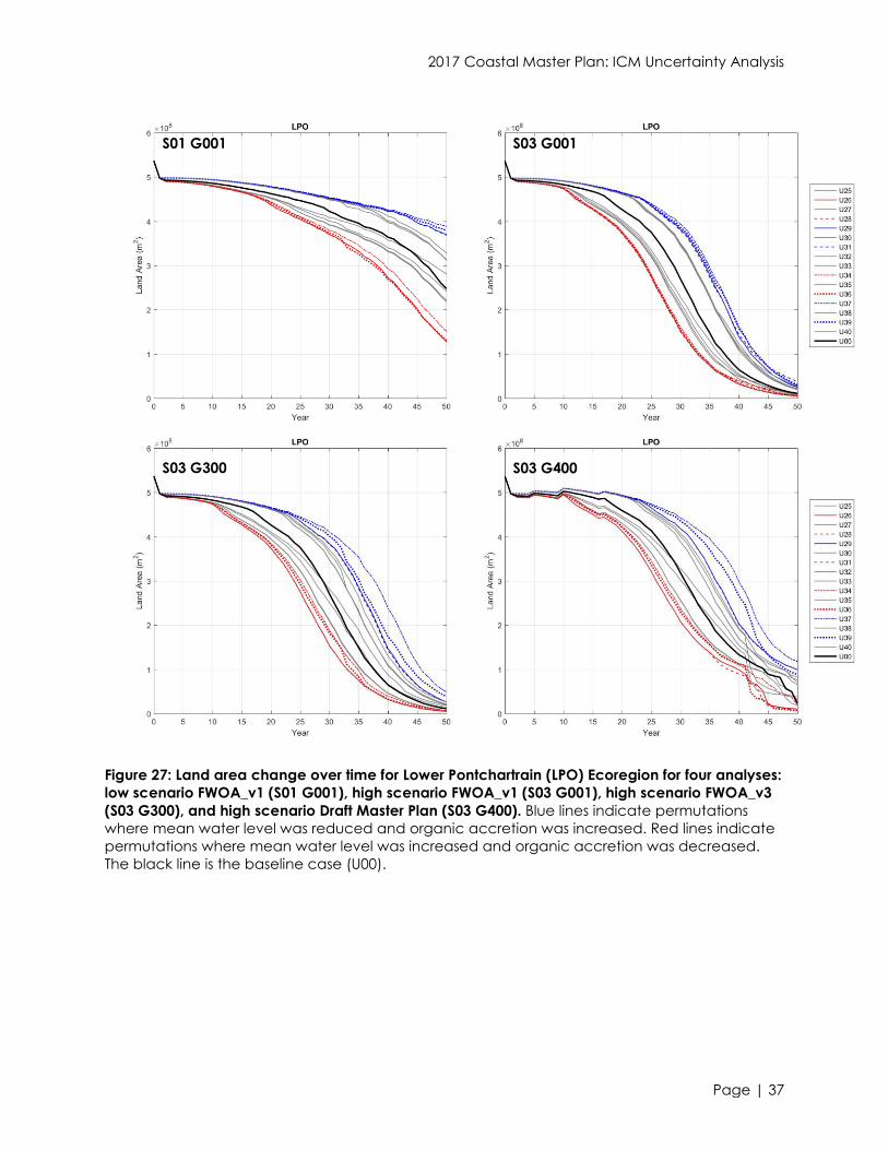
2017 Coastal Master Plan: ICM Uncertainty Analysis
Page | 37
Figure 27: Land area change over time for Lower Pontchartrain (LPO) Ecoregion for four analyses:
low scenario FWOA_v1 (S01 G001), high scenario FWOA_v1 (S03 G001), high scenario FWOA_v3
(S03 G300), and high scenario Draft Master Plan (S03 G400). Blue lines indicate permutations
where mean water level was reduced and organic accretion was increased. Red lines indicate
permutations where mean water level was increased and organic accretion was decreased.
The black line is the baseline case (U00).
S01 G001 S03 G001
S03 G300 S03 G400

2017 Coastal Master Plan: ICM Uncertainty Analysis
Page | 38
Figure 28: Land area change over time for Breton (BRT) Ecoregion for four analyses: low scenario
FWOA_v1 (S01 G001), high scenario FWOA_v1 (S03 G001), high scenario FWOA_v3 (S03 G300),
and high scenario Draft Master Plan (S03 G400). Blue lines indicate permutations where mean
water level was reduced and organic accretion was increased. Red lines indicate permutations
where mean water level was increased and organic accretion was decreased. The black line is
the baseline case (U00).
S01 G001 S03 G001
S03 G300 S03 G400

2017 Coastal Master Plan: ICM Uncertainty Analysis
Page | 39
Figure 29: Land area change over time for Bird’s Foot Delta (BFD) Ecoregion for four analyses: low
scenario FWOA_v1 (S01 G001), high scenario FWOA_v1 (S03 G001), high scenario FWOA_v3 (S03
G300), and high scenario Draft Master Plan (S03 G400). Blue lines indicate permutations where
mean water level was reduced and organic accretion was increased. Red lines indicate
permutations where mean water level was increased and organic accretion was decreased.
The black line is the baseline case (U00).
S01 G001 S03 G001
S03 G300 S03 G400

2017 Coastal Master Plan: ICM Uncertainty Analysis
Page | 40
Figure 30: Land area change over time for Upper Barataria (UBA) Ecoregion for four analyses: low
scenario FWOA_v1 (S01 G001), high scenario FWOA_v1 (S03 G001), high scenario FWOA_v3 (S03
G300), and high scenario Draft Master Plan (S03 G400). Blue lines indicate permutations where
mean water level was reduced and organic accretion was increased. Red lines indicate
permutations where mean water level was increased and organic accretion was decreased.
The black line is the baseline case (U00).
S01 G001 S03 G001
S03 G300 S03 G400

2017 Coastal Master Plan: ICM Uncertainty Analysis
Page | 41
Figure 31: Land area change over time for Lower Barataria (LBA) Ecoregion for four analyses: low
scenario FWOA_v1 (S01 G001), high scenario FWOA_v1 (S03 G001), high scenario FWOA_v3 (S03
G300), and high scenario Draft Master Plan (S03 G400). Blue lines indicate permutations where
mean water level was reduced and organic accretion was increased. Red lines indicate
permutations where mean water level was increased and organic accretion was decreased.
The black line is the baseline case (U00).
S01 G001 S03 G001
S03 G300 S03 G400

2017 Coastal Master Plan: ICM Uncertainty Analysis
Page | 42
Figure 32: Land area change over time for Lower Terrebonne (LTB) Ecoregion for four analyses:
low scenario FWOA_v1 (S01 G001), high scenario FWOA_v1 (S03 G001), high scenario FWOA_v3
(S03 G300), and high scenario Draft Master Plan (S03 G400). Blue lines indicate permutations
where mean water level was reduced and organic accretion was increased. Red lines indicate
permutations where mean water level was increased and organic accretion was decreased.
The black line is the baseline case (U00).
S01 G001 S03 G001
S03 G300 S03 G400

2017 Coastal Master Plan: ICM Uncertainty Analysis
Page | 43
Figure 33: Land area change over time for Atchafalaya/Teche/Vermilion (AVT) Ecoregion for four
analyses: low scenario FWOA_v1 (S01 G001), high scenario FWOA_v1 (S03 G001), high scenario
FWOA_v3 (S03 G300), and high scenario Draft Master Plan (S03 G400). Blue lines indicate
permutations where mean water level was reduced and organic accretion was increased. Red
lines indicate permutations where mean water level was increased and organic accretion was
decreased. The black line is the baseline case (U00).
S01 G001 S03 G001
S03 G300 S03 G400

2017 Coastal Master Plan: ICM Uncertainty Analysis
Page | 44
Figure 34: Land area change over time for Mermentau/Lakes (MEL) Ecoregion for four analyses:
low scenario FWOA_v1 (S01 G001), high scenario FWOA_v1 (S03 G001), high scenario FWOA_v3
(S03 G300), and high scenario Draft Master Plan (S03 G400). Blue lines indicate permutations
where mean water level was reduced and organic accretion was increased. Red lines indicate
permutations where mean water level was increased and organic accretion was decreased.
The black line is the baseline case (U00).
S01 G001 S03 G001
S03 G300 S03 G400

2017 Coastal Master Plan: ICM Uncertainty Analysis
Page | 45
Figure 35: Land area change over time for Calcasieu/Sabine (CAS) Ecoregion area for four
analyses: low scenario FWOA_v1 (S01 G001), high scenario FWOA_v1 (S03 G001), high scenario
FWOA_v3 (S03 G300), and high scenario Draft Master Plan (S03 G400). Blue lines indicate
permutations where mean water level was reduced and organic accretion was increased. Red
lines indicate permutations where mean water level was increased and organic accretion was
decreased. The black line is the baseline case (U00).
S01 G001 S03 G001
S03 G300 S03 G400

2017 Coastal Master Plan: ICM Uncertainty Analysis
Page | 46
Figure 36: Land area change over time for Eastern Chenier Ridge (ECR) Ecoregion for four
analyses: low scenario FWOA_v1 (S01 G001), high scenario FWOA_v1 (S03 G001), high scenario
FWOA_v3 (S03 G300), and high scenario Draft Master Plan (S03 G400). Blue lines indicate
permutations where mean water level was reduced and organic accretion was increased. Red
lines indicate permutations where mean water level was increased and organic accretion was
decreased. The black line is the baseline case (U00).
S01 G001 S03 G001
S03 G300 S03 G400

2017 Coastal Master Plan: ICM Uncertainty Analysis
Page | 47
Figure 37: Land area change over time for Western Chenier Ridge (WCR) Ecoregion for four
analyses: low scenario FWOA_v1 (S01 G001), high scenario FWOA_v1 (S03 G001), high scenario
FWOA_v3 (S03 G300), and high scenario Draft Master Plan (S03 G400). Blue lines indicate
permutations where mean water level was reduced and organic accretion was increased. Red
lines indicate permutations where mean water level was increased and organic accretion was
decreased. The black line is the baseline case (U00).
S01 G001 S03 G001
S03 G300 S03 G400
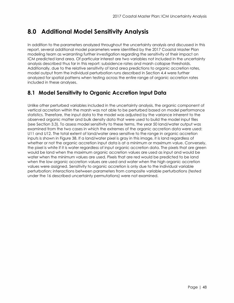
2017 Coastal Master Plan: ICM Uncertainty Analysis
Page | 48
8.0 Additional Model Sensitivity Analysis
In addition to the parameters analyzed throughout the uncertainty analysis and discussed in this
report, several additional model parameters were identified by the 2017 Coastal Master Plan
modeling team as warranting further investigation regarding the sensitivity of their impact on
ICM predicted land area. Of particular interest are two variables not included in the uncertainty
analysis described thus far in this report: subsidence rates and marsh collapse thresholds.
Additionally, due to the relative sensitivity of land area predictions to organic accretion rates,
model output from the individual perturbation runs described in Section 4.4 were further
analyzed for spatial patterns when testing across the entire range of organic accretion rates
included in these analyses.
8.1 Model Sensitivity to Organic Accretion Input Data
Unlike other perturbed variables included in the uncertainty analysis, the organic component of
vertical accretion within the marsh was not able to be perturbed based on model performance
statistics. Therefore, the input data to the model was adjusted by the variance inherent to the
observed organic matter and bulk density data that were used to build the model input files
(see Section 3.3). To assess model sensitivity to these terms, the year 50 land/water output was
examined from the two cases in which the extremes of the organic accretion data were used:
U11 and U12. The total extent of land/water area sensitive to the range in organic accretion
inputs is shown in Figure 38. If a land/water pixel is gray in this image, it is land regardless of
whether or not the organic accretion input data is at a minimum or maximum value. Conversely,
the pixel is white if it is water regardless of input organic accretion data. The pixels that are green
would be land when the maximum organic accretion values are used as input and would be
water when the minimum values are used. Pixels that are red would be predicted to be land
when the low organic accretion values are used and water when the high organic accretion
values were assigned. Sensitivity to organic accretion is only due to the individual variable
perturbation; interactions between parameters from composite variable perturbations (tested
under the 16 described uncertainty permutations) were not examined.

2017 Coastal Master Plan: ICM Uncertainty Analysis
Page | 49
Figure 38: All land under low scenario FWOA using ICM_v1 that is sensitive to individual
perturbation of organic accretion inputs. Any land/water pixel that is green was water at year 50
when the low value of organic accretion is used (U12) and was land at year 50 when the high
value of organic accretion was used (U11). Red represents pixels predicted to be land when the
low value of organic accretion was used and land when the high organic accretion values were
used.
8.2 Model Sensitivity to Subsidence Rates
As part of the development of the environmental scenarios used for the 2017 Coastal Master
Plan, numerous subsidence rates were tested in the ICM. A full discussion of these analyses is
provided in Appendix C: Modeling, Chapter 2: Future Scenarios. Of the five candidate scenarios
developed under that analysis, three of the scenarios all utilized the same eustatic sea level rise
rate (0.63 m over 50 years). These three scenarios (S02, S04, and S05) were all identical with the
exception of the subsidence rates used; three different subsidence rates were tested: 20%, 35%
and 50% into the range of subsidence observations. A subsidence rate of “20% into the range”
indicates that the subsidence rate was set to a value that was 20% between the minimum and
maximum observed rate for a given subsidence zone. For example if the observed data ranged
from 5 mm/yr to10 mm/yr, 20% into the range would be a rate of 6 mm/yr, 35% would be 6.75
mm/yr, and 50% into the range would be a rate of 7.5 mm/yr. Since everything except
subsidence rate was held constant for these three runs, the spatial patterns of model sensitivity
to subsidence rates can be shown.

2017 Coastal Master Plan: ICM Uncertainty Analysis
Page | 50
Figure 39: Sensitivity range in land predicted at year 50 under the low subsidence rate (S04: 20%)
and the medium subsidence rate (S05: 35%). Any land/water pixel that is red was water at year
50 when the medium subsidence rate was used and was land at year 50 when the low
subsidence rate was used. Green represents pixels that are predicted as land when the medium
subsidence rate was used and water when the low subsidence rate was used.

2017 Coastal Master Plan: ICM Uncertainty Analysis
Page | 51
Figure 40: Sensitivity range in land predicted at year 50 under the medium subsidence rate (S05:
35%) and the high subsidence rate (S02: 50%). Any land/water pixel that is red was water at year
50 when the high subsidence rate was used and was land at year 50 when the medium
subsidence rate was used. Green represents pixels that are predicted as land when the high
subsidence rate was used and water when the medium subsidence rate was used.

2017 Coastal Master Plan: ICM Uncertainty Analysis
Page | 52
Figure 41: Sensitivity range in land predicted at year 50 under the low subsidence rate (S04: 20%)
and the high subsidence rate (S02: 50%). Any land/water pixel that is red was water at year 50
when the high subsidence rate was used and was land at year 50 when the low subsidence rate
was used. Green represents pixels that are predicted as land when the high subsidence rate was
used and water when the low subsidence rate was used.
With respect to model uncertainties tested and discussed in this report, it appears that the model
sensitivity to subsidence rates tested and used for the master plan modeling are of the same
magnitude (or greater) than the uncertainties in model output introduced by the perturbations
defined by model performance statistics.
8.3 Model Sensitivity to Marsh Collapse Thresholds
The marsh collapse thresholds used in the 2017 Coastal Master Plan analyses were chosen based
on the coast wide mean inundation that coincides with vegetated biomass that is two standard
deviations below the mean biomass (as represented by the normalized vegetation index)
(Couvillion & Beck, 2013). The 2012 Coastal Master Plan Marsh Collapse Threshold Advisory Panel
analyzed this same data and provided inundation values for each coastal basin, which were
more variable than the coast wide averages ultimately used (in both 2012 and 2017) (CPRA,
2011). To assess model sensitivity, the extreme values for each marsh type from all coastal basins
were used as the inundation collapse thresholds (Table 5). Additionally, sensitivity of fresh marsh
to salinity collapse was assessed by adjusting the length of time used to define the maximum
salinity. The model sensitivity was tested with the following seven conditions:
1. Adjust intermediate marsh threshold down (use High Collapse Inundation Threshold)
2. Adjust intermediate marsh threshold up (use Low Collapse Inundation Threshold)

2017 Coastal Master Plan: ICM Uncertainty Analysis
Page | 53
3. Adjust brackish marsh threshold down (use High Collapse Inundation Threshold)
4. Adjust brackish marsh threshold up (use Low Collapse Inundation Threshold)
5. Adjust salt marsh threshold down (use High Collapse Inundation Threshold)
6. Adjust salt marsh threshold up (use Low Collapse Inundation Threshold)
7. Adjust fresh marsh collapse to use growing season salinity (consistent with 2012 models)
rather than two-week mean salinity
Table 5: Inundation collapse thresholds used to assess model sensitivity. Original analysis
summarized in Table 2 of the 2012 Marsh Collapse Threshold Advisory Panel Summary Report.
Collapse thresholds are the depth of inundation (meters) over the marsh surface in which the
marsh will still survive. Persistent inundation deeper than this threshold depth will result in wetland
collapse.
Original Inundation
Threshold Value Used
in 2017 Coastal
Master Plan
Low Collapse Inundation
Threshold from 2012 Marsh
Collapse Threshold Panel
Report
High Collapse Inundation
Threshold from 2012 Marsh
Collapse Threshold Panel
Report
Intermediate 0.358 m 0.443 m 0.140 m
Brackish 0.256 m 0.386 m 0.190 m
Saline 0.235 m 0.399 m 0.135 m
As evident in the following figures, the model sensitivity to the range in collapse thresholds is
spatially variable as a result of the predominant vegetation in a given area. Due to the fact that
saline marsh is the predominant vegetation type in later decades, it is intuitive that the range in
predicted land area at year 50 is most sensitive across the range of saline marsh collapse
thresholds (Figure 42).

2017 Coastal Master Plan: ICM Uncertainty Analysis
Page | 54
Figure 42: Sensitivity range in land predicted at year 50 under the extreme saline marsh collapse
threshold values. Pixels that are green are predicted as land when saline marshes are more
inundation tolerant and predicted as water when saline marshes are less tolerant to inundation.
Red represents pixels that are predicted as water when saline marshes are more inundation
tolerant and predicted as land when saline marshes are less inundation tolerant.
Brackish marsh is the second most prevalent type of vegetation at year 50, and the model
sensitivity to the brackish marsh inundation threshold is similarly less than the sensitivity to the
saline marsh inundation threshold range (Figure 43). Following this same trend, intermediate
marsh is even less prevalent at year 50 in the model and therefore the model is least sensitive to
the intermediate marsh inundation threshold (Figure 44).

2017 Coastal Master Plan: ICM Uncertainty Analysis
Page | 55
Figure 43: Sensitivity range in land predicted at year 50 under the extreme brackish marsh
collapse threshold values. Pixels that are green are predicted as land when brackish marshes
are more inundation tolerant and predicted as water when brackish marshes are less tolerant to
inundation. Red represents pixels that are predicted as water when brackish marshes are more
inundation tolerant and predicted as land when brackish marshes are less inundation tolerant.

2017 Coastal Master Plan: ICM Uncertainty Analysis
Page | 56
Figure 44: Sensitivity range in land predicted at year 50 under the extreme intermediate marsh
collapse threshold values. Pixels that are green are predicted as land when intermediate
marshes are more inundation tolerant and predicted as water when intermediate marshes are
less tolerant to inundation. Red represents pixels that are predicted as water when intermediate
marshes are more inundation tolerant and predicted as land when intermediate marshes are
less inundation tolerant.
The final marsh collapse variable tested in this sensitivity analysis was the salinity value used to
define the collapse-inducing salinity in fresh wetland regions. For the 2017 Coastal Master Plan,
the maximum two-week mean salinity of the year is used to define the salinity value in which
fresh wetlands may experience salinity stress. This was updated from the 2012 Coastal Master
Plan, which used the annual mean salinity to define the collapse-inducing salinity. Therefore, by
comparing land area from these two approaches, it can be shown as to what portion of the
model domain is subjected to very short periods of salinity stress that result in land loss. By year
50, this is mostly evident in the upper regions of Terrebonne and Barataria (Figure 45), which are
both prone to periodic salinity spikes in later simulation years due to higher sea level and
periodic droughts during summer months.

2017 Coastal Master Plan: ICM Uncertainty Analysis
Page | 57
Figure 45: Sensitivity range in land predicted at year 50 under the different fresh marsh salinity
stress collapse routines. Pixels that are green are predicted as land when the annual mean
salinity is used to define the stress-inducing salinity and predicted as water when the maximum
two-week mean salinity of the year was used.
As shown in these sensitivity analysis simulations, the final extent of land area predicted by the
ICM is fairly sensitive to the marsh collapse threshold values chosen for a given simulation. The
analysis conducted for the 2012 Coastal Master Plan produced spatially variable representations
of marsh inundation that could be operationalized in future simulations for a more complex
representation of marsh collapse; however, regardless of spatially variability in collapse threshold
values, the utilization of a collapse threshold methodology still represents an inherently dynamic
and complex process with a relatively simple Boolean operator. Incorporation of the marsh
collapse thresholds into the relative sea level rise scenarios approach (as was essentially done in
the 2012 effort), may be an appropriate path forward if a more dynamic wetland collapse
process is unable to be operationalized in future efforts.
9.0 Summary and Conclusions
This uncertainty analysis was based on applying perturbations to model variables that are
directly linked to the calculations of land area. These model variables included water level,
water level variability, salinity, TSS concentration, and organic accretion. The perturbations were
applied to each of these variables before they were used in subsequent model subroutines.
These perturbations were consistently applied through the 50-year simulations, and the
magnitude of the perturbation of each variable was estimated based on the calibration errors.
Perturbing wetland types were not examined here as they were controlled by the prevailing
hydrologic conditions, and as such were removed from further consideration.

2017 Coastal Master Plan: ICM Uncertainty Analysis
Page | 58
A set of experiments were designed to examine the perturbation of individual variables. The
individual perturbations showed that water level and organic accretion have the most influence
on land area. Salinity showed an influence on the wetland type but not on land area, while TSS
showed minor influence on land area.
Additional composite experiments were performed to examine simple addition of uncertainties
originating from individual perturbations. Further, and to fully examine the interdependency
among the model variables, a set of 16 experiments was performed. These experiments
provided a bracket of uncertainty around the FWOA baseline run. The results show that water
level and organic accretion are the most influential on the coast wide land area.
Additional simulations were performed to examine the uncertainty in the calculations of land
area under conditions identical to the scenarios used to formulate the 2017 Coastal Master Plan.
The uncertainty in land prediction under a future with the Draft 2017 Coastal Master Plan
implemented on the landscape was also assessed. Overall, the uncertainty in land area
predicted increases over time under a low relative sea level rise scenario FWOA and decreases
under a higher relative sea level rise scenario as any uncertainty from model error is overtaken
by the extreme sea level rise rates. Once the Draft 2017 Coastal Master Plan is implemented,
there is substantially more land throughout the model domain, as compared to FWOA. This
increase in land area results in the Draft 2017 Coastal Master Plan permutations not converging
upon the asymptotic lower limit as seen in the FWOA permutations. This subsequently leads to a
larger uncertainty range than the FWOA permutations. Overall, and as seen in Figure 25, under
all conditions, the Draft 2017 Coastal Master Plan results in more land area than the FWOA.
Many model input parameters were not able to be perturbed by the methodology followed for
the uncertainty analysis, in which model performance errors were used to assign a perturbation
factor to model outputs. The modeling team determined that the ICM prediction of land area at
year 50 seemed to be particularly sensitive to three such parameters: subsidence rates, organic
matter accretion, and marsh collapse threshold values. The spatial extent of model-predicted
land area changed substantially due to setting these variables at extreme values. Of the marsh
collapse threshold values, the year 50 prediction of land area within the model domain was
most sensitive to the saline marsh inundation-induced collapse threshold; a finding in agreement
with the fact that the majority of land remaining at year 50 under the medium scenario is saline
marsh. The extent of land impacted by the total range tested in subsidence rates and organic
matter input rates were roughly the same magnitude as the saline marsh collapse threshold. The
land area predicted at year 50 was not as sensitive to collapse thresholds for brackish,
intermediate, or fresh marsh types.

2017 Coastal Master Plan: ICM Uncertainty Analysis
Page | 59
10.0 References
Burkett, V., Groat, C.G. and Reed, D. (2007). Hurricanes not the key to a sustainable coast.
Science, 315,1366–1367.
Chai, T. and Draxler, R.R. (2014). Root mean square error (RMSE) or mean absolute error (MAE)? –
Arguments against avoiding RMSE in the literature. Geoscience Model Development, 7,
1247–1250.
Couvillion, B., and Beck, H. (2013). Marsh collapse thresholds for coastal Louisiana estimated
using elevation and vegetation index data. Journal of Coastal Research, 63, 58-67.
CPRA. (2011). CPRA 2012 Master Plan Update: Marsh Collapse Threshold Advisory Panel. LDNR La
Salle Building, Griffon Room, held on January 31, 2011.
Habib, E. and Reed, D.J. (2013). Parametric Uncertainty Analysis of Predictive Models in
Louisiana's 2012 Coastal Master Plan. Journal of Coastal Research: Special Issue 67 -
Louisiana′s 2012 Coastal Master Plan Technical Analysis, 127–146.
Willmott, C.J. and Matsuura, K. (2005). Advantages of the mean absolute error (MAE) over the
root mean square error (RMSE) in assessing average model performance. Climate
Research, 30, 79–82.