Embed Size (px)
DESCRIPTION
VALUE CHAIN OPTIMIZATION OF A FOREST BIOMASS POWER PLANT CONSIDERING UNCERTAINTIES
Citation preview

VALUE CHAIN OPTIMIZATION OF A FOREST BIOMASS POWER PLANT
CONSIDERING UNCERTAINTIES
by
Nazanin Shabani
B.Sc., Civil Engineering, Sharif University of Technology, 2003
M.Sc., Civil Engineering, Iran University of Science and Technology, 2005
M.A.Sc., Civil Engineering, University of British Columbia, 2009
A THESIS SUBMITTED IN PARTIAL FULFILLMENT OF
THE REQUIREMENTS FOR THE DEGREE OF
DOCTOR OF PHILOSOPHY
in
The Faculty of Graduate and Postdoctoral Studies
(Forestry)
THE UNIVERSITY OF BRITISH COLUMBIA
(Vancouver)
April 2014
© Nazanin Shabani, 2014

ii
Abstract
Mathematical modeling has been employed to improve the cost competitiveness of forest
bioenergy supply chains. Most of the studies done in this area are at the strategic level, focus on
one part of the supply chain and ignore uncertainties. The objective of this thesis is to optimize
the value generated in a forest biomass power plant at the tactical level considering uncertainties.
To achieve this, first the supply chain configuration of a power plant is presented and a nonlinear
model is developed and solved to maximize its overall value. The model considers procurement,
storage, production and ash management in an integrated framework and is applied to a real case
study in Canada. The optimum solution forecasts $1.74M lower procurement cost compared to
the actual cost of the power plant. Sensitivity analysis and Monte Carlo simulation are performed
to identify important uncertain parameters and evaluate their impacts on the solution.
The model is reformulated into a linear programming model to facilitate incorporating
uncertainty in the decision making process. To include uncertainty in the biomass availability,
biomass quality and both of them simultaneously, a two-stage stochastic programming model, a
robust optimization model and a hybrid stochastic programming-robust optimization model are
developed, respectively. The results show that including uncertainty in the optimization model
provides a solution which is feasible for all realization of uncertain parameters within the defined
scenario sets or uncertainty ranges, with a lower profit compared to the deterministic model.
Including uncertainty in biomass availability using the stochastic model decreases the profit by
$0.2M. In the robust optimization model, there is a trade-off between the profit and the selected
range of biomass quality. Profit decreases by up to $3.67M when there are ±13% variation in
moisture content and ±5% change in higher heating value. The hybrid model takes advantage of

iii
both modeling approaches and balances the profit and model tractability. With the cost of only
$30,000, an implementable solution is provided by the hybrid model with unique first stage
decision variables. These models could help managers of a biomass power plant to achieve
higher profit by better managing their supply chains.

iv
Preface
This dissertation is original and presents the work of Nazanin Shabani during her Ph.D. program.
The research was conducted by the author under the supervision of her academic adviser, Dr.
Taraneh Sowlati. Dr. Sowlati advised Shabani during the process of defining the research topic,
gathering data and information, developing and validating the models and preparing manuscripts.
This thesis presents a background on the research topic, research objectives, a review of the
literature, several optimization models to achieve the research objectives with their application to
a real case study in Canada, analysis of the obtained results, and the main findings and
conclusions. The author visited the power plant several times, had close collaboration with the
managers of the power plant, obtained information and detailed data on the power plant supply
chain, presented the model results to the power plant managers and had the model validated by
them. Five scientific papers were generated from this research, and in all of them Shabani was
the first author. The list of papers generated from this research is provided below.
A version of Chapter 2 is published. Shabani, N., Akhtari, S., Sowlati, T. 2013. Value chain
optimization of forest biomass for bioenergy production: A review. Renewable and
Sustainable Energy Reviews, 110(3): 280-290.
A version of Chapter 3 is published. Shabani N, Sowlati T. 2013. A mixed integer non-linear
programming model for tactical value chain optimization of a wood biomass power plant.
Applied Energy, 104:353-361.
A version of Chapter 4 is submitted for publication. Shabani N, Sowlati T.Evaluating the
impact of uncertainty and variability on the value chain optimization of a forest biomass
power plant using Monte Carlo Simulation.

v
A version of Chapter 5 is submitted for publication. Shabani N, Sowlati T., Ouhimmou M.,
Rönnqvist M. Tactical supply chain planning for a forest biomass power plant under supply
uncertainty.
A version of Chapter 6 is submitted for publication. Shabani N, Sowlati T. A hybrid
stochastic programming-robust optimization model for maximizing the value chain of a
forest biomass power plant under uncertainty.
vi
Table of Contents
Abstract ........................................................................................................................................... ii
Preface............................................................................................................................................ iv
Table of Contents ........................................................................................................................... vi
List of Tables ................................................................................................................................. ix
List of Figures ................................................................................................................................ xi
Acknowledgements ...................................................................................................................... xiii
Dedication ..................................................................................................................................... xv
Chapter 1 Introduction .................................................................................................................. 1
1.1 Background ...................................................................................................................... 1
1.2 Research objectives .......................................................................................................... 6
1.3 Organization of the dissertation ....................................................................................... 7
Chapter 2 Literature review ........................................................................................................... 9
2.1 Synopsis ........................................................................................................................... 9
2.2 Deterministic optimization models .................................................................................. 9
2.2.1 Power plants ............................................................................................................ 10
2.2.2 District heating plants ............................................................................................. 13
2.2.3 Co-generation plants ............................................................................................... 16
2.2.4 Biofuel plants .......................................................................................................... 20
2.3 Optimization models with uncertainties ......................................................................... 23
2.3.1 Modeling approaches .............................................................................................. 27
2.3.2 Sensitivity analysis and Monte Carlo simulation.................................................... 31
2.3.3 Stochastic programming ......................................................................................... 34
2.3.4 Robust optimization model ..................................................................................... 38

vii
2.4 Discussion and conclusions ............................................................................................ 41
Chapter 3 Deterministic model ................................................................................................... 43
3.1 Synopsis ......................................................................................................................... 43
3.2 The power plant supply chain ........................................................................................ 43
3.3 The optimization model ................................................................................................. 49
3.4 Case study ...................................................................................................................... 55
3.5 Results ............................................................................................................................ 60
3.5.1 Scenario analysis ..................................................................................................... 61
3.5.2 Sensitivity analysis.................................................................................................. 63
3.6 Discussion and conclusions ............................................................................................ 65
Chapter 4 Monte Carlo simulation .............................................................................................. 68
4.1 Synopsis ......................................................................................................................... 68
4.2 Uncertainty and Monte Carlo simulation ....................................................................... 68
4.2.1 Uncertainty in biomass quality ............................................................................... 70
4.2.2 Uncertainty in biomass availability and cost and electricity price ......................... 76
4.3 Results ............................................................................................................................ 77
4.4 Discussion and conclusions ............................................................................................ 82
Chapter 5 Stochastic programming ............................................................................................. 85
5.1 Synopsis ......................................................................................................................... 85
5.2 The mixed integer programming model of the power plant supply chain ..................... 85
5.3 The stochastic mixed integer programming model of the power plant supply chain .... 88
5.4 Managing the risk ........................................................................................................... 92
5.4.1 Variability index ..................................................................................................... 93
5.4.2 Downside risk ......................................................................................................... 94
5.5 Results ............................................................................................................................ 95

viii
5.5.1 Result of deterministic models................................................................................ 95
5.5.2 Results of the stochastic model ............................................................................... 95
5.5.3 Results for the variability index ............................................................................ 101
5.5.4 Results for the downside risk ................................................................................ 103
5.6 Discussion and conclusions .......................................................................................... 103
Chapter 6 Hybrid stochastic programming-robust optimization model .................................... 106
6.1 Synopsis ....................................................................................................................... 106
6.2 Robust optimization formulation ................................................................................. 106
6.3 Hybrid stochastic programming-robust optimization model ....................................... 111
6.4 Results .......................................................................................................................... 113
6.5 Discussion and conclusions .......................................................................................... 118
Chapter 7 Conclusions, strength points, limitations and future research .................................. 121
7.1 Conclusions .................................................................................................................. 121
7.2 Strengths points ............................................................................................................ 122
7.3 Limitations ................................................................................................................... 124
7.4 Future research ............................................................................................................. 125
References ................................................................................................................................... 127

ix
List of Tables
Table 2-1: Summary of studies on deterministic optimization of forest biomass power plants ... 13
Table 2-2: Summary of studies on deterministic optimization of district heating plants ............. 15
Table 2-3: Summary of studies on deterministic optimization of co-generation plants ............... 19
Table 2-4: Summary of studies on deterministic optimization of biofuel plants .......................... 23
Table 2-5: Summary of studies on sensitivity analysis, scenario analysis and Monte Carlo
simulation applied to bioenergy supply chain with uncertainty ................................................... 33
Table 2-6: Summary of studies on stochastic programming of forest and bioenergy supply chains
....................................................................................................................................................... 38
Table 2-7: Summary of studies on robust optimization of forest and bioenergy supply chain .... 41
Table 3-1: List of indices and decision variables used in the optimization model ....................... 49
Table 3-2: List of parameters used in the optimization model ..................................................... 50
Table 3-3: Characteristics of the case study ................................................................................. 56
Table 3-4: Variables and parameters of the case study ................................................................. 58
Table 3-5: Results of cost, revenue and profit for the optimization model (in $M) ..................... 60
Table 3-6: Total profit and biomass procurement cost for four different scenarios ..................... 63
Table 4-1: Product type of suppliers and their contract type ........................................................ 70
Table 4-2: Average and standard deviation of bark, sawdust and shavings MC for Suppliers 1 to
5..................................................................................................................................................... 71
Table 4-3: Average and standard deviation of biomass MC for Supplier 6 ................................. 73
Table 4-4: Average and standard deviation of HHV for different biomass types ........................ 75
Table 4-5: Minimum, maximum, average and standard deviation of profit for considering
uncertainty in different parameters ............................................................................................... 78
Table 4-6: Results of Monte Carlo simulation-optimization model for scenarios of electricity
price and biomass availability and cost ........................................................................................ 79
Table 4-7: Probability of having profit within different ranges when considering uncertainty in
different model parameters ........................................................................................................... 81

x
Table 4-8: Ranges of biomass purchase from suppliers without contract, biomass consumption
and storage levels when considering uncertainty in different parameters (1000 green tonnes) ... 82
Table 5-1: Decision variables of the linear programming model ................................................. 85
Table 5-2: Stochastic model decision variables ............................................................................ 90
Table 5-3: Expected value of profit for scenario analysis, stochastic and average scenario models
($M) .............................................................................................................................................. 96
Table 5-4: Biomass procurement cost for each scenario of stochastic and deterministic models
($M) .............................................................................................................................................. 99
Table 5-5: Average profit if the first stage decision variables of each scenario is implemented
and other scenarios happen ($M) ................................................................................................ 100
Table 5-6: Average and standard deviation of the monthly biomass consumption for
deterministic model with scenario analysis and stochastic models (1000 green tonnes) ........... 101
Table 6-1: Profit ($M) for different ranges of MCs,p,t and HHVs,p,t used in the robust optimization
model........................................................................................................................................... 114
Table 6-2: Profit for different ranges of MCs,p,t and HHVs,p,t used in the robust optimization and
hybrid models.............................................................................................................................. 118

xi
List of Figures
Figure 3-1: Schematic of supply chain configuration of a forest biomass power plant ............... 43
Figure 3-2: The amount of firm and surplus electricity production in each month ...................... 61
Figure 3-3: Optimum amount of biomass stored, purchased and consumed in each month based
on the 2011 data ............................................................................................................................ 61
Figure 3-4: Variations in profit with 20% change in different parameters ................................ 64
Figure 3-5: Variations in profit for different initial storage levels ............................................... 64
Figure 4-1: Histogram and probability distribution of MC of bark (a), sawdust (b), shavings (c)72
Figure 4-2: Histogram and probability distribution for MC of RLD in January (a), February (b),
March (c), April (d), June (e), July (f), August (g), September (h), October (i), November (j), and
December (k) ................................................................................................................................ 75
Figure 4-3: Histogram and probability distribution of HHV of sawdust (a) and RLD (b) ........... 76
Figure 4-4: Histogram of profit when MC varies ......................................................................... 78
Figure 4-5: Histogram of profit when HHV varies ....................................................................... 78
Figure 4-6: Histogram of profit when electricity price and biomass availability and cost vary for
a) low, b) average and c) high scenarios ....................................................................................... 80
Figure 5-1: Histogram of profit distribution for the deterministic model with first stage decisions
based on average scenario and the stochastic model .................................................................... 97
Figure 5-2: Profit mean and standard deviation for different weights (ρ) .................................. 102
Figure 5-3: Histogram of profit distribution for different weights (ρ) associated with variability
index ............................................................................................................................................ 102
Figure 5-4: Histogram of profit distribution for before and after managing the downside risk
(Ω=$14M) ................................................................................................................................... 103
Figure 6-1: Solution of the robust optimization model for different ranges of moisture content114
Figure 6-2: Solution of the robust optimization model for different ranges of higher heating value
..................................................................................................................................................... 115
Figure 6-3: Solution of the robust optimization model for different ranges of energy value ..... 115
Figure 6-4: The optimum storage level in different months from the robust optimization model
with HHVs,p,t∈[8100,8900] and MCs,p,t∈[26,34] and the deterministic model ........................... 116

xii
Figure 6-5: The optimum biomass consumption level in different months from the robust
optimization model with HHVs,p,t∈[8100,8900] and MCs,p,t∈[26,34] and the deterministic model
..................................................................................................................................................... 117
Figure 6-6: Optimum storage level of 27 scenarios for the first five months for a) robust
optimization model, and b) hybrid stochastic programming-robust optimization model when
HHVs,p,t∈[8100,8900] and MCs,p,t∈[26,34] ................................................................................ 118

xiii
Acknowledgements
First of all, I offer my enduring gratitude to my dear supervisor, Dr. Taraneh Sowlati, for her
help, guidance, and consideration during my Ph.D. studies. She put endless effort into
supervising and motivating me, and never seemed to be tired or reluctant to help. Her enthusiasm
and dedication for research always inspire me.
I am indeed grateful to my supervisory committee, Dr. Farrokh Sassani and Dr. Philip D. Evans
for their time and invaluable feedback on my research during my PhD studies. Special thanks to
Dr. John D. Nelson, Dr. Harish Krishnan and Dr. Chander K. Shahi for critically reviewing the
thesis and providing constructive comments on it. I am also grateful to Dr. Mustapha Ouhimmou
and Dr. Mikael Rönnqvist for their comments and collaboration on reformulating the non-linear
model to a linear model presented in Chapter 5.
I would also like to thank the Natural Sciences and Engineering Research Council of Canada
(NSERC) for providing the funding for this research. I also acknowledge the partial funding
provided by the power plant and sincerely thank the Fiber Supply Manager and Finance Manager
for their time and support in providing the required data and information for the modeling and
validating the results.
I express my appreciation to my lab-mates and friends in the Industrial Engineering Research
Group for their comments and discussion during my Ph.D. studies. I am also thankful of my
friends at UBC for their kindness and support during my stay in Canada and creating so much
fun in my life. Special thanks to my dear friend, Nina, who assisted me in proofreading the
thesis.

xiv
I would like to express my deepest gratitude to my beloved family in Iran. My sincere
appreciation is due to my lovely parents for their unconditional love and support throughout my
life.
Last but not least, I express my profound affection and appreciation to my love and my best
friend, Hamid, for his continuous love, kindness, encouragement and support during my years of
education. This accomplishment would not have been done without him.

xv
Dedication
To my mother, Faranak, who taught me how to be happy by immersing myself in every
joyful moment of my life.
To my father, Mohammad, my polestar, who cultivated in me a hunger for learning.

1
Chapter 1 Introduction
1.1 Background
Using forest biomass as an energy source is not a new idea; before the twentieth century, wood
was one of the main sources of energy, but it has been substituted partly by coal, oil and natural
gas during the past century (Bowyer et al., 2007). Recently, there has been an interest in the
utilization of more sustainable and secure energy sources such as forest biomass due to the high
levels of emissions associated with fossil fuels, increasing energy demands and volatility of
international energy market (Ragauskas et al., 2006).
Biomass is defined as biological material derived from living, or recently living organisms.
Depending on the source of biomass, there are three main biomass categories: forest (woody)
biomass, agricultural biomass, and bio-wastes (animal waste and municipal solid waste)
(Rentizelas et al., 2009b). This research focuses on utilizing forest biomass to generate
electricity in power plants using direct combustion.
Although the conversion and transportation of forest biomass for energy generation affects the
air quality negatively (Hall & Scrase, 1998), there is a potential to decrease emissions
significantly when it is used as a substitute for fossil fuels (Hall (2002), Ahtikoski et al. (2008),
International Energy Agency (2012)). Generally, if managed (produced, transported and used)
in a sustainable manner, converting biomass to energy or fuel is considered to be a carbon
neutral process, meaning that the amount of CO2 released during biomass combustion is equal
to the amount of CO2 taken from the atmosphere by the plant during the growing stage (Saidur
et al., 2011). Increasing the contribution of biomass in energy generation is an important step in
developing sustainable communities, managing greenhouse gas emissions effectively according

2
to Ragauskas et al. (2006), and decreasing the gap between the actual emission levels and the
international protocol targets such as those in the Kyoto and Copenhagen Accords (Bradley D.,
2010). In areas covered with large forest lands and large forest industries, such as Canada, a
large amount of forest biomass is available for energy generation (Bradley D., 2010). In
Canada, after hydro, biomass has the highest share in the production of renewable energy
(2.9% in 2008 according to Ralevic (2008)).
Forest biomass is a flexible energy source, capable of generating electricity, heat, biofuels or a
combination of them. Compared to other renewable energy sources such as wind or solar, the
advantage of using forest biomass for energy generation is that it can be stored and used on
demand (Hall & Scrase (1998), Demirbaş (2001)). It also has the potential to: increase the
recovery of forest residues that would otherwise be disposed of in landfills or incinerated,
create jobs, and provide local and sustainable energy for communities which in turn will
decrease their dependency on the international fuel market (BIOCAP Canada, 2008).
Forest biomass for the purpose of energy generation can be supplied from forest residues
including branches and tops left in the harvest areas, by-products of other forest product mills,
such as sawdust, bark and shavings (Demirbaş, 2001), and fast growing crops such as poplar
and willow grown specifically for energy purposes (Rockwood et al., 2004). Chipping,
handling, transporting, storing and pre-processing operations, such as drying for improving the
quality of biomass, are usually needed before using forest biomass for energy generation
(Flisberg et al., 2012). Forest biomass can be used for energy generation either directly, such as
in direct heat and power generation, or indirectly such as in biofuels (pellet, bioethanol)
production. The energy production process depends on the conversion technology used in the

3
energy plant (Rentizelas et al., 2009b). The conversion technologies include pelletization,
combustion, co-combustion, gasification, pyrolysis, digestion and fermentation (Demirbaş
(2001), Frombo et al. (2009a)). Different types of products are then sent to customers through
the grid, networks or channels of distributors, wholesalers and retailers. Profit in each stage of
the forest bioenergy supply chain is a function of procurement, transportation, operating,
capital and other costs, and depends also on the availability and quality of biomass (Gunn,
2009).
Despite the advantages of using forest biomass for energy generation, there are several barriers
to its efficient utilization, including biomass availability, cost and quality, conversion
efficiency, transportation cost, and the efficiency of the supply logistics system. Forest biomass
is a bulky material with relatively low density (400-900 kg/m3 (Demirbaş, 2001)) and high
moisture content (Hall, 2002). The quality of raw material plays an important role in the
performance of the production process (Rentizelas et al., 2009b). It is difficult to collect,
transport, handle and store low-density materials. Moreover, unlike fossil fuels, forest biomass
is usually spread over large areas rather than being concentrated. Transportation could
contribute as much as 50% to the total biomass cost in some cases (Allen et al., 1998) and may
involve the use of a large amount of equipment and different transportation modes (Hall &
Scrase, 1998). Inaccessibility of forests in some months during the year, when energy demand
is quite high, raises concerns about the secure supply of biomass to energy plants. Therefore,
storage, which affects the quality of material (Fuller, 1985), is also important in this supply
chain. Comminution and storage of residues can take place either in the forest, at the plant or at
an intermediate point. Another challenge in using forest biomass for energy generation is the
existence of uncertainty in this supply chain due to several factors, such as market instability,

4
natural disasters, policy and climate change as well as the nature of the industry (for example
heterogeneous raw material and unpredictable quality (Hall, 2002)). Uncertainty makes this
supply chain volatile and risk vulnerable, which in turn makes proper planning difficult.
All these challenges contribute to a higher cost of energy generation from forest biomass
compared to that of other sources of energy. Utilizing more advanced technologies, for
example to improve raw material quality or system efficiency, is one way to deal with some of
these challenges. A complementary approach to reduce the cost of energy produced from forest
biomass and increase its competitiveness is to improve its supply chain and optimize its design
and production planning (Bowyer et al., 2007).
A supply chain model can be developed to help decision makers in their decisions and manage
the supply chain more efficiently. Operations research and mathematical programming have
been used in forest biomass supply chain planning and management. Modeling is effective
particularly if it integrates different parts of the supply chain, such as procurement, production,
transportation, and distribution, and at different decision levels, such as strategic, tactical and
operational levels. Using optimization techniques in designing and managing forest bioenergy
supply chains could result in better performance which could help to make this energy source
economically viable according to Bowyer et al. (2007).
Optimization models have been developed and used in the literature to determine the optimal
material flow, transportation, storage and chipping location of energy systems, mainly heating
plants (Eriksson & Björheden (1989), Gunnarsson et al. (2004), Kanzian et al. (2009), Freppaz
et al. (2004) and Van Dyken et al. (2010)). There are also some studies that evaluated the
conversion technology and the possibility of co-generation in the design of district heating

5
systems using mathematical programming (Nagel (2000), Frombo et al. (2009a), Difs et al.
(2010), Wetterlund & Söderström (2010), Börjesson & Ahlgren (2010) and Keirstead et al.
(2012)). Biomass supply chains for generating biofuels have also been studied (Chinese &
Meneghetti (2009), Ekşioğlu et al. (2009), Kim et al. (2011a), and a iba e -Aguilar et al.
(2011)). Although using forest biomass for electricity generation is not as common as using it
for generating heat, there are some studies that considered the supply chain design of biomass
power plants in an optimization framework, i.e. Reche et al. (2008), Alam et al. (2009 and
2012a) and Vera et al. (2010). These studies focused on the strategic design of a forest
biomass power plant and did not consider the tactical planning with multiple time steps in their
models. Alam et al. (2012b) suggested an optimization model for biomass procurement to meet
the monthly electricity demand of a forest biomass power plant over a one-year time horizon.
Decision variables of the model included monthly harvesting levels from several forest cells.
This study focused on the procurement of biomass and did not include the whole supply chain
in an integrated framework. Moreover, none of the above mentioned studies included the
impact of biomass quality on the electricity production and its cost. Specifically, the quality of
different types of biomass in different months of the year, the quality of the mix of biomass in
the storage and the impact of storing biomass on the amount and cost of generated electricity
have not been studied previously.
There are some studies in the literature that consider uncertainty in biofuel supply chain
optimization models. Some of them evaluated the impact of uncertainty on the model solution
through sensitivity analysis and Monte Carlo simulation (Kim et al. (2011a), Rauch & Gronalt
(2011)). More advanced optimization techniques that incorporate uncertainty in the modeling,
e.g. stochastic programming (Kim et al. (2011b), Chen & Fan (2012), Awudu & Zhang (2013),

6
Kazemzadeh & Hu (2013)) and robust optimization (Tay et al. (2013), Bredström et al.
(2013)), have also been used in this supply chain. Uncertainty in the supply chain of forest
biomass power plants and its effect on electricity production cost are ignored in previous
studies. Alam et al. (2012b) have only addressed uncertainty in the supply chain of a forest
biomass power plant through sensitivity analysis and concluded that the impact of uncertainty
in moisture content on the production cost was significant. However, there is no study in this
area that include uncertainty into the decision making process. Instead, optimization models in
the literature provided results only based on the expected value of the uncertain parameters.
Ignoring uncertainty in deterministic optimization models may result in non-optimal and/or
infeasible solutions for real world case studies. Hence, optimization models need to be
extended to incorporate uncertainty and variations in the input parameters of the supply chain.
1.2 Research objectives
The main objective of this research is to develop tools (models) to help managers of biomass
power plants to achieve greater efficiencies (profit) by better managing their supply chains,
especially by considering uncertainty in the supply chain. The specific objectives of this study
are as follows:
1. To optimize the supply chain of a forest biomass power plant considering biomass
supply, storage and electricity production in an integrated framework. To achieve this
objective a new mathematical programming model is developed to provide decisions on
the amount of biomass to be purchased, stored and consumed in each month over a one-
year time horizon to maximize the profit.
2. To apply the developed model to a real case study in Canada.

7
3. To evaluate the impact of changes in uncertain parameters on the solution of the
mathematical programming model. This objective is achieved by examining historical
data and performing sensitivity analysis, scenario analysis and Monte Carlo simulation.
4. To incorporate uncertainty in different parameters into the supply chain decision
making process. This objective is reached by developing stochastic programming and
robust optimization models, and a hybrid model. Using different modeling approaches
allowed the inclusion of uncertainty in different parameters, i.e. biomass quality and
availability. The hybrid model should incorporate uncertainties in different parameters
in the model simultaneously.
1.3 Organization of the dissertation
In addition to the introduction chapter, this dissertation includes a chapter on the literature
review, a chapter on the deterministic optimization model, a chapter on the Monte Carlo
simulation model, a chapter on stochastic programming model, a chapter on hybrid stochastic
programming-robust optimization model and a chapter on conclusions, limitations of the study,
and suggestions for future research.
The previous studies on forest bioenergy supply chain in the literature are discussed in Chapter
2. They are categorized based on the inclusion of uncertainty.
In Chapter 3, an optimization model is proposed for the supply chain planning of a forest
biomass power plant over one year. Later in this Chapter, the model is applied to a real case
study in Canada and different scenarios are evaluated and sensitivity analysis is also performed
to assess the impact of different scenarios as well as variations in input parameters on the
generated profit.

8
Monte Carlo simulation along with the optimization model is performed and presented in
Chapter 4 to provide the ranges of generated profit and its distribution when input parameters
vary. Historical data on input parameters (biomass quality, cost, availability and electricity
price) as well as data analysis are presented in this Chapter. From the results of the Monte
Carlo simulation model, risks of having low profit and low or high storage levels associated
with uncertainty in model parameters are identified.
In Chapter 5, uncertainty in the available monthly supply is incorporated in the decision
making by developing a two-stage stochastic model and two different risk measures, variability
index and downside risk, are also considered.
In Chapter 6, uncertainty in biomass quality is also added to the decision making process
through developing a robust optimization model. Then, a hybrid stochastic programming-
robust optimization model is proposed to include uncertainty in different parameters
simultaneously. The final conclusions, strengths and limitations of the study and some
suggestions for future research are presented in the last chapter, Chapter 7.

9
Chapter 2 Literature review
2.1 Synopsis
In several previous studies, optimization techniques have been employed to manage the forest
bioenergy supply chain for heat, electricity and biofuels production from strategic, tactical and
operational points of view. Most of these studies were deterministic and ignored uncertainty,
while there are examples that included uncertainty in the supply chain models especially during
the past few years. This chapter covers major relevant studies on optimization of forest
bioenergy supply chains. It also discusses the issue of uncertainty in this supply chain,
uncertainty sources and the methods used for dealing with it. The studies are categorized into
two groups: 1) studies that used deterministic mathematical programming for modeling forest
bioenergy supply chains, and 2) studies that considered uncertainty in the analysis of forest
biomass supply chains. Studies that used deterministic models are categorized based on the
type of bioenergy plants into those related to power plants, district heating plants, co-
generation plants and biofuel plants. Studies that considered uncertainty are categorized based
on the modeling approaches. Some examples from other forest product industries as well as
other biofuel industries that included uncertainty in their supply chain optimization are also
presented. The strengths and shortcomings of the relevant literature are highlighted at the end
of this chapter.
2.2 Deterministic optimization models
Different optimization techniques, such as linear programming (LP) and mixed integer linear
programming (MILP), have been used for supply chain design and management. LP is a
mathematical method which includes a set of variables to be determined, a linear objective
function to be optimized, and a set of linear equality or inequality constraints to be met. The

10
main advantages of using this optimization method are its ability to solve large scale problems,
its assured convergence to global optimum solutions, having no need to have an initial solution
and its use of a well-developed duality theory for sensitivity analysis and the ease of problem
formulation (Labadie, 1997). If some of the variables in LP are integers, the model is called
mixed integer linear programming (MILP). In this section, the studies that optimized the supply
chain of electricity plants, district heating systems, co-generation plants and biofuel plants
using forest biomass are reviewed.
2.2.1 Power plants
Forest biomass can be used in power plants directly or in combination with fossil fuels for
generating electricity. It can be burnt at a constant rate in a boiler furnace to heat water and
produce steam. The steam is then carried through the furnace using pipes to raise its
temperature and pressure further. Finally, the steam passes through the multiple blades of a
turbine, spinning the shaft, which runs an electricity generator which produces an alternating
current to use locally or to supply the national grid (Demirbaş, 2001).
The optimal supply area and location of a forest biomass power plant in a distributed power
generation system was determined by Reche et al. (2008). The objective function was to
maximize the profitability index as a function of the net present value of benefits from the sale
of electrical energy minus the initial investment, collection, transportation, maintenance and
operating costs. The authors used an artificial intelligence method, called particle swarm
optimization. They concluded that it is important in distributed generation systems to consider
the technical constraints of the network and the voltage regulation. Finally, they evaluated the
model performance using simulation.

11
Alam et al. (2009) constructed a three–objective model for optimizing the amount of each
individual type of biomass from each of the harvesting zones, and then applied their model to a
50 MWh biomass power plant using both harvesting residues and poplar trees collected from
three management zones in Northwestern Ontario, Canada. To optimize the supply chain of
energy plants, it is sometimes necessary to formulate a problem with more than one objective
since single objective models cannot always represent the problem accurately. The objectives
are often in conflict (minimizing and maximizing objectives) and it might not be possible to
achieve an optimal solution that optimizes all the objectives simultaneously. In this situation,
the trade-off between objectives can be shown and the most efficient solution is selected. In
Alam et al. (2009), pre-emptive goal programming was applied to give priority to the
objectives as follows: 1) minimizing the procurement cost of feedstock, 2) minimizing the
transportation distance of biomass supply to the plant, and 3) minimizing the feedstock
moisture content. Alam et al. (2012b) developed a GIS based integrated optimization model to
optimize the supply chain of the forest biomass power plant with 230 MW capacity. The power
plant was fed by two biomass types: harvesting residues (leftover tops, branches and other parts
of the trees harvested mainly for lumber and pulp and paper industries) and unutilized biomass
(non-merchantable trees, and trees damaged by wildfire, wind and insects). GIS data were used
to estimate transportation costs from each forest cell to the power plant. The decision variables
were the harvest levels of two types of woody biomass in each month. The objective function
was to minimize the total piling, processing, felling, extraction and transportation costs.
Finding the optimal size, location, supply area and net present value of an electricity plant in
Spain was studied in Vera et al. (2010). The raw material of the power plant was olive tree
pruning residues and the technology for electricity generation was gasifier with gas turbine.

12
The authors used GIS data for the location and number of olive trees per km2, roads,
topographical features, electric line locations, etc. Different plant sizes and locations were
considered and the optimal one with the highest net present value was determined using three
metaheuristic methods. These methods were Genetic Algorithms (GA), Binary Honey Bee
Foraging (BHBF) and Binary Particle Swarm Optimization (BPSO). It was concluded that
BHBF algorithm converged to the optimal solution better than BPSO and GA. The results
indicated that the optimal plant size was 2 MW and the predicted optimal location of the plant
was in the area with highest available biomass.
Pérez-Fortes et al. (2014) developed an optimization model to determine location-allocation
and the selection/capacity of different pre-treatment technologies for feeding biomass to an
already existing coal combustion power plant. They included biomass transportation and
storage in their model. Different pre-treatments technologies were considered including
torrefaction, torrefaction combined with pelletization, pelletization, fast pyrolysis and fast
pyrolysis combined with char grinding. Changes in biomass quality (moisture content, dry
matter, energy density and bulk density) through the use of pretreatment processes were also
studied.
Table 2-1 summarizes the studies on optimization models used for modeling forest biomass
power plant supply chain.

13
Table 2-1: Summary of studies on deterministic optimization of forest biomass power plants
Author-Year-
Region Objective Function Decision Variables Method
Reche et al.
(2008)
Spain
Maximizing profitability index (net
present value of revenue from selling
electricity minus initial investment,
biomass collection and transportation
costs, and maintenance and operation
costs)
Location and supply area
of the biomass power plant
Particle
swarm
optimization
Vera et al.
(2010) Spain
Maximizing net present value (revenue
from the sale of electrical energy minus
initial investment and collection,
transportation, maintenance and operation
costs)
Plant size and location
Supply area
Several
metaheuristic
methods
Alam et al.
(2009)
Canada
Minimizing total biomass procurement
cost
Minimizing total distance for procurement
of biomass
Maximizing the quality of biomass
(minimizing moisture content)
Quantity of biomass
procured from each supply
location to each plant
Biomass procurement zone
selection (Binary variable)
Multi
Objective
Programming
Alam et al.
(2012b)
Canada
Minimize the total piling, processing,
felling, extraction and transportation
costs.
The harvest levels of two
types of woody biomass in
each month
Non-linear
dynamic
programming
Pérez-Fortes
et al. (2014)
Spain
Minimizing net present value of
investment and operational costs
Maximizing the environmental impact of
adding biomass to a coal power plant
Location/allocation and
selection/capacity of pre-
treatment technology
Fraction of coal replaced
by biomass
Material flow
Multi-
objective
Mixed
Integer
Programming
(MIP)
2.2.2 District heating plants
Forest biomass for energy generation is mainly used in district heating systems. These systems
consist of a central plant producing heat which is sent to a group of users (customers) through a
network of pipelines in the form of hot water or steam (Gilmour & Warren, 2007). Several
authors developed optimization models for supply chain design and management of heating

14
plants. Eriksson & Björheden (1989) developed a model with decision variables related to
storage and the chipping locations for a heating plant. Gunnarsson et al. (2004) developed a
mixed integer programming model for tactical-strategic supply chain management of forest
fuel used in a heating plant in Sweden by focusing on supply procurement decisions rather than
the production process. Multiple time steps were considered in this model. It was used to solve
six generated problems rather than being applied to a real case study. The results of using
different solution methods (LP and IP, and IP heuristic) to solve the problems were compared
in this work. Strategic decisions such as plant size and location were studied in Chinese &
Meneghetti (2005) and Schmidt et al. (2010). The most profitable configuration (plant size) of
a multi-source biomass district heating plant in Italy was considered in Chinese & Meneghetti
(2005). The model developed by Kanzian et al. (2009) included 16 combined heat and power
plants and 8 terminal storages in Austria. Optimum locations of bio-energy plants were studied
in Schmidt et al. (2010) with a case study in Austria. In another study, done by Van Dyken et
al. (2010), a linear mixed-integer model was developed for biomass supply chains with
transportation, storage and processing operations over 12 weekly time steps considering
supply, constant demand, three different biomass products and two demand loads for chips and
heat. This study focused on operational supply chain planning and the developed model was
not applied to a real case study. A truck scheduling optimization model was developed in Han
& Murphy (2012) for transportation of four types of forest biomass to energy plants in Oregon,
US. This study only considered the transportation part of the supply chain.
Table 2-2 summarizes all of these studies with their objective functions and decision variables.

15
Table 2-2: Summary of studies on deterministic optimization of district heating plants
Author -Year-
Region Objective Function Decision Variables Method
Eriksson &
Björheden
(1989)
Sweden
Minimizing forest biomass
supply cost (chipping, storing
and transportation costs)
Flow of biomass direct or via storage
Chipping location
Linear
Programming
(LP)
Nagel (2000)
Germany
Maximizing annual profit
(revenue from sale of energy
minus investment cost, fixed
and variable costs, fuel cost
and waste disposal cost)
Level of heat produced by each
boiler at each time period
The capacity of the system
Whether or not to integrate a boiler
into the heating system (Binary
variable)
Mixed Integer
Programming
(MIP)
Gunnarsson et
al. (2004)
Sweden
Minimizing biomass supply
cost (transportation, chipping
and storage costs)
Flow of biomass within the supply
network
Quantity of biomass chipped and
stored at roadside and terminal
If biomass is forwarded to or is
chipped at each roadside location,
each sawmill is contracted or not,
each terminal is used or not (Binary
variables)
Mixed Integer
Programming
(MIP)
Chinese &
Meneghetti
(2005)
Italy
Maximizing profit (revenues
from sale of energy and
charging customers with
connection fees minus boiler
investment, construction and
operating costs)
Heat produced by each boiler at each
time period
The capacity of the system
If a boiler would integrate to the
heating system or not (Binary
variable)
Mixed Integer
Programming
(MIP)
Frombo et al.
(2009a) Italy
Maximizing net annual profit
(revenue from sale of heat
and power minus felling and
processing, skidding,
highway transportation, plant
installation and management
costs)
Annual quantity of biomass
harvested from each supply area
The plant capacity for different
conversion technologies
Linear
Programming
(LP)

16
Author -Year-
Region Objective Function Decision Variables Method
Frombo et al.
(2009b) Italy
Maximizing net annual profit
(revenue from sale of heat
and power minus felling and
processing, skidding,
highway transportation, plant
installation and management
costs)
The quantity of biomass harvested at
each harvesting location and to be
used at each plant location.
The capacity of each plant
Selection of the conversion
technology (Binary variables)
Mixed Integer
Programming
(MIP)
Kanzian et al.
(2009) Austria
Minimizing biomass supply
cost to the heating plants
(chipping, storing and
transporting costs)
Volume of wood chips transported
from each terminal to each plant
Location of terminals and plants
(Binary variable)
Mixed Linear
Programming
(MIP)
Van Dyken et
al. (2010)
Norway
Minimizing the present value
of the costs (investment and
operating costs and salvage
value)
Biomass, product and energy flow
within the supply network
Emissions from storing and drying
biomass
Biomass input and output moisture
content to and from dryer
Biomass storage duration (Binary
variable)
Linear and
Mixed Integer
Programming
(LP and MIP)
Keirstead et
al. (2012) UK
Minimizing system cost
(biomass purchase, storage,
transportation and conversion
costs)
Optimal capacity of boilers
Whether chipped forest biomass
should be imported from neighbor
area or non-chipped residues should
be imported and then chipped within
the area (Binary variable)
Mixed Integer
Programming
(MIP)
Han &
Murphy
(2012) US
Minimize the weighted sum
of transportation costs
Minimize the total working
time
Truck schedules Simulated
Annealing
2.2.3 Co-generation plants
Combined heat and power (CHP) systems are energy plants that use cogeneration technology
to produce both heat and power in a district heating system (Gilmour & Warren, 2007). In
some studies, mathematical programming was used to compare the cost of generating either
energy or biofuels from biomass and evaluate the possibility of co-generation.

17
Some studies indicated that utilizing biomass for energy generation is more cost effective than
for biofuel production. Azar et al. (2003) concluded that utilizing biomass for generating heat
was the most economical scenario. Wahlund et al. (2004) showed that using wood biomass for
pelletization would have a lower cost and higher CO2 reduction than using it for biofuel
production. Feng et al. (2010) investigated the possibility of having bioenergy facilities (they
called them biorefineries) in typical existing sawmills, pulp and paper mills, wood panel
facilities, biochemical, energy, and pellet facilities. Then, the authors developed a
mathematical model to design this integrated supply chain optimally.
A methodology for optimizing the utilization of distributed biomass resources for energy
production was proposed by Alfonso et al. (2009). The main focus of the paper was to optimize
the logistics, but economic and environmental analyses of different bioenergy alternatives were
also performed. The authors indicated that the methodology would provide the optimal
locations of the biomass plant, energy application (electricity, heat and/or standardized biofuels
such as pellets), and the employed technology. This methodology was applied to three districts
in Spain. Based on the results, the authors concluded that the shortest payback period and
highest CO2 savings were attained from cogeneration plants, followed by pellet plants. The
least ranked option was power-only power plants.
Difs et al. (2010) analyzed different biomass gasification scenarios, and determined the
optimum configuration with the current fossil fuel price and green energy policies. Wetterlund
& Söderström (2010) considered two scenarios of co-generating Synthetic Natural Gas (SNG)
and district heat, and co-generation of heat and power. The authors determined the policy
support levels (tradable biofuel certificates) that would make the SNG scenario cost
competitive with CHP, while maximizing the annual profit over a 20-year time period. The

18
cost-effectiveness of different applications of biomass gasification was analyzed by Börjesson
& Ahlgren (2010). The focus of this study was to determine whether CHP generation in
biomass integrated gasification combined cycle (BIGCC) plants, and biofuels production in
biomass gasification biorefineries in a case study in Sweden were cost efficient. Schmidt et al.
(2010) used a mixed integer linear programming model for optimizing the location of
bioenergy plants using forest biomass in Austria. The bioenergy plants included integrated
gasification combined cycle (IGCC) system and biomass CHP plants with carbon capture
storage (CCS), pellet mill, and transportation fuel (methanol and ethanol) plants.
The problem of indicating whether to produce electricity in addition to heat at biomass
combustion plants was studied by Freppaz et al. (2004). A decision support system (DSS) was
presented by Rentizelas et al. (2009a) to optimize a multi-biomass energy conversion system to
generate electricity, heating and cooling in an area in Greece. The authors concluded that
considering multi-biomass supply chain reduced the cost by decreasing warehousing
requirements, especially for seasonal types of biomass. The developed model was non-linear
and a hybrid optimization method was used to solve that. Rauch & Gronalt (2011) developed a
model for designing a forest fuel CHP plant supply chain in Austria.
The summary of studies on modeling co-generation plants is provided in Table 2-3.

19
Table 2-3: Summary of studies on deterministic optimization of co-generation plants
Author- Year-
Region Objective Function Decision Variables Product Method
Freppaz et al.
(2004) Italy
Maximizing annual profit
(revenues from sale of
energy minus harvesting,
transportation, installation
and maintenance, and
energy distribution costs)
Annual quantity of biomass
harvested at each collection
area and transported from
each collection area to each
of six district energy systems
Capacity and the percentage
of thermal energy generated
at each plants
If the plant produces
electricity or not (Binary
variable)
Heat/
Electricity
Mixed
Integer
Programming
(MIP)
Alfonso et al.
(2009) Spain
Minimize transport
duration, optimize the
location, etc.
Biomass resources, logistics
structure, bioenergy plants
size and location, technology
type, etc.
Co-
generation
Did not
mention
Rentizelas et
al. (2009a)
Greece
Maximizing the financial
yield of the investment
Location and size of the
bioenergy facility
The biomass types and
quantities
The maximum collection
distance for each type
Co-
generation
Hybrid
optimization
Börjesson &
Ahlgren
(2010)
Sweden
Not discussed in the paper
The optimal production
capacity at different subsidy
levels.
Selection of alternative
technologies for district heat
generation (Binary variable)
Biofuel/
Heat
Mixed
Integer
Programming
(MIP)
Difs et al.
(2010)
Sweden
Maximizing annual profit
(revenues from sale of
energy products minus
investment, fuel and
maintenance costs)
Capacity of new investment
Selection of investment
alternatives for future
(Binary variable)
Co-
generation
Mixed
Integer
Programming
(MIP)

20
Author- Year-
Region Objective Function Decision Variables Product Method
Schmidt et al.
(2010)
Austria
Minimizing total cost of
energy generation (costs of
biomass supply and
transportation, energy
generation, carbon capture
and storage, plant building
and distribution network
investment and
distribution)
The annual amount of
energy commodities
produced at plants: heat,
power, pellets, and
transportation fuels.
Plant size and location,
pipeline networks selection
and district heating networks
selection (Binary variables)
Fuel/
Energy
Mixed
Integer
Programming
(MIP)
Wetterlund &
Söderström
(2010)
Sweden
Maximizing annual profit
(revenues from sale of
electricity and synthetic
natural gas minus
investment, fuel and
maintenance costs)
The optimal government
support level (subsidy)
Selection of new investment
alternatives (Binary
variable)
Co-
generation
Mixed
Integer
Programming
(MIP)
Rauch &
Gronalt
(2011)
Austria
Minimizing total
procurement cost
(transport, chipping
investment, operations and
maintenance costs)
The annual volume of fuel
transported between
districts, terminals, regional
departure railway, and the
CHP plant
Open or close a terminal
(binary variable)
CHP
Mixed
Integer
Programming
(MIP)
2.2.4 Biofuel plants
Bioethanol is a type of fuel that is extracted from biomass through fermentation (Limayem &
Ricke, 2012). The bioethanol production has increased in recent years in many countries, such
as the U.S. Although most of the bioethanol is produced from agricultural biomass, the
controversial issue of using plants as fuel instead of food made it necessary to look for more
acceptable sources, namely forest biomass (Limayem & Ricke, 2012). Generating biofuels
from forest biomass is still in the developing phase and has not been commercialized yet. The
main challenges in commercialization of this technology include high energy or chemical
consumption for woody biomass pretreatment, even when compared to agricultural biomass,

21
low system efficiency, process scalability and intensive capital investment (Zhu & Pan, 2010).
In most of the studies presented here, forest biomass combined with agricultural biomass was
used for biofuel production
Some previous studies considered biomass supply chain management for generating biofuels.
Chinese & Meneghetti (2009) considered a real-life problem of supplying a biofuel plant with
forest fuel. A mixed-integer linear programming model was proposed to determine the optimal
configuration of the supply chain. It was mentioned that the model could be useful in resolving
trade-offs between decentralized early treatment of biofuels, resulting in lower transportation
costs, and centralized final treatment, allowing to reap the benefits of economies of scale. It
was therefore advised to apply integrated supply chain planning concepts to design biofuel
logistics systems and to support policy making in the energy field. An MIP model was also
developed by Ekşioğlu e al. (2009) for designing the biorefinery supply chain producing
cellulosic ethanol from agricultural and woody biomass. The model outputs were the number,
size and location of biorefinery plants with the objective of minimizing the total cost of annual
harvesting, storing, transporting and processing biomass; storing and transporting ethanol; and
locating and operating bio-refineries. The model included constraints on biomass availability,
flow, conversion, production and inventory capacities, and demand. The data from the State of
Mississippi was used to validate the model. The author concluded that transportation costs,
biomass availability, technology type, and planting and harvesting costs are important factors
in supply chain design decisions.
Kim et al. (2011a) developed a mixed integer linear programming optimization model for the
supply chain design of bio-gasoline and biodiesel production from six forestry resources
(logging residuals, thinnings, prunings, inter-cropped grasses, and chips/shavings). The first set

22
of conversion plants could be from a set of candidate sites with four capacity options to convert
biomass to three product types: bio-oil, char and fuel gas. These intermediate products could be
used either as local fuel sources or as feedstock to produce final products (gasoline and
biodiesel) at the second conversion plants, which could be from a set of candidate sites with
four capacity options. There were several possible markets for the final products with certain
maximum demands. The objective of the model was to maximize the overall profit by
determining the number, location, and size of the conversion plants, biomass supply locations,
the logistics and the amount of materials to be transported between the various nodes of the
designed network, while satisfying the demand constraints. The considered case study was
based on an industrial database related to a case in the Southeastern United States. The authors
evaluated the trade-off between centralized and distributed network designs.
The trade-off between economic and environmental objectives in the optimal planning of a
biorefinery in Mexico was evaluated in a iba e -Aguilar et al. (2011). The authors used a
multi-objective optimization model for selecting the feedstock type, processing technology,
and a set of products in a biorefinery supply chain. The raw material contained different types
of agricultural biomass, wood chips, sawdust, commercial wood for producing ethanol,
hydrogen, and biodiesel (generated only from agricultural biomass). The objectives were: 1) to
maximize the profit considering the costs of feedstock, products, and processing, and 2) to
minimize the life cycle environmental impacts. The authors applied their model to a case study
in Mexico. The decision makers could select from the output the solutions that fit the specific
requirements and compensate for both objectives simultaneously.
Table 2-4 summarizes the studies on optimization models used for modeling the supply chain
of forest biofuel plants.

23
Table 2-4: Summary of studies on deterministic optimization of biofuel plants
Author-Year-
Region Objective Function Decision Variables Method
Chinese &
Meneghetti
(2009) Italy
Minimizing total cost of
supply chain (harvesting,
transportation, processing
and facility installation
costs)
Flow of biomass within the supply
network
Whether to use a preprocessing
equipment or not (Binary variable)
Mixed Integer
Programming
(MIP)
Ekşioğlu e al.
(2009) USA
Minimizing total annual
cost (investment,
harvesting, storing and
transportation costs)
Number, size, and location of bio-
refineries required
Quantity of biomass harvested,
shipped, processed and stored
Whether a biorefinery and a collection
facility with specific size are located
in each site (Binary variables)
Mixed Integer
Programming
(MIP)
Kim et al.
(2011) US
Maximizing the overall
profit
Number, location, and size of the
conversion plants
Biomass supply locations
Logistics and the amount of materials
to be transported between the various
nodes of the designed network
Mixed Integer
Programming
(MIP)
a iba e -
Aguilar et al.
(2011)
Mexico
Maximizing profit (revenue
from sale of products minus
investment, process,
operating and transportation
costs)
Minimizing environmental
impacts
The quantity of products produced
from different biomass feedstock
using different processing routes
The quantity of each biomass
feedstock used for producing different
products through different processing
routes
Multi-objective
Programming
2.3 Optimization models with uncertainties
Uncertainty refers to the lack of information or the lack of certainty in the validity of the
information about the existing or future state of a system (Kangas & Kangas, 2004). It can
result from measurement errors and ignorance, which is to some extent inevitable and might be
reduced by further studies or investing in improved technology to acquire high quality data
(Petrovic (2001), Ells et al. (1997)). It may result from variability in random future events due

24
to their inherent nature (such as feedstock characteristics) (Bowyer et al. 2012), which can be
controlled to some extend by employing better forecasting methods and/or using expert
judgment. It can also result from lack of reliable historical data or lack of certainty in historical
data, for example lack of data on the demand of a new product. Other sources of uncertainty
include imprecision in judgment, vagueness, and ambiguity related to the known objects, which
belong to poorly defined sets so they cannot be classified well (Kangas & Kangas (2004),
Petrovic (2001), Ells et al. (1997)). From the system boundary point of view, the source of
uncertainty may exist outside the production process, called environmental uncertainty, such as
uncertainty in demand and supply. It may also be within the production process, called system
uncertainty, such as uncertainty in lead time due to machine failure (Chrwan-JYH, 1989). In
terms of time horizon, uncertainty may be the result of short term variations, such as day-to-
day processing variations, cancelled/rushed orders and equipment failure, or long-term
variations, such as raw material/final product unit price fluctuations, seasonal demand
variations and technology changes. Therefore, uncertainty exists in supply chains at strategic,
tactical and operational levels and should be considered in supply chain decisions.
There are several reasons why uncertainties exist in the biomass supply chain. Some of the
sources of uncertainty in forest biomass supply chains are similar to those in other industries,
such as economic fluctuation and instability, raw material supplies, manufacturing process
time, machine breakdowns, reliability of transportation channels, and exchange rates. However,
there are other sources of uncertainty that are related specifically to the characteristics of forest
biomass supply chains which are summarized here:
Interdependency between different forest sectors: There are interdependencies between
different sectors and markets within the forest industry supply chains. This means that
25
raw material of one sector could be the product of another sector. Consequently,
variations in one part of the supply chain usually propagate into the other parts.
Variations in feedstock supply: The need for having a continuous supply of raw
material for a bioenergy facility necessitates the use of a mixture of materials or even to
have new sources of material. Even when one type of biomass is used for energy
production, the quality of biomass varies over time. Therefore, this industry must have
a dynamic supply chain.
Wood is a heterogeneous natural material: Its physical and chemical characteristics
affect the quality and quantity of the products (Bowyer et al. 2012). In the bioenergy
industry, the moisture content and heating value of raw material play an important role
in the amount of produced energy and its costs (Saidur et al., 2011). Heating value and
moisture content vary from one tree stands or species to another (Demirbaş (2001),
Carlsson et al. (2009), Demirbaş (2003)) and also differ in different types of biomass
(e.g. bark, sawdust, shavings) (Lehtikangas, 2001). Wood properties may be affected by
external factors, such as growth condition, climate, harvesting methods, storage and
transportation methods. Biomass quality, such as moisture content, can also change
during storage, production, and transportation.
Divergent production structure: Unlike most of other manufacturing industries, which
have an assembly structure, forest products industries generally have a divergent
production structure. This means that multiple products, by-products, and co-products
are made from a single product simultaneously. Consequently, it is difficult to
completely control the manufacturing processes. Moreover, it is challenging to forecast
the quality and quantity of outputs due to this production structure and the use of

26
heterogeneous natural raw material in the production. This fact can impact the amount
of raw material available for bioenergy plants, which are supplied by other forest
product mills.
Ambiguous values and objectives: Most forest areas include large areas with diverse
geographical and ecological characteristics. In forestry, it is usually needed to
i corpora e differe values a d s akeholders’ prefere ces a d i eres s which
sometimes cannot be understood, interpreted or quantified completely (Ells et al.,
1997). Therefore, it is likely to have vague factors, values and objectives which can also
exist in the forest bioenergy supply chain. This aspect of uncertainty cannot be dealt
with like other sources of uncertainty. To some extent, it is possible to spend time and
money in some form of consulting with the stakeholders to get a better understanding of
their preferences, opinions, and values. However, sometimes the stakeholders may not
be able to express their preferences before a specific decision is made.
New markets and new production technologies: Investment grants, carbon and energy
taxes, green certificate schemes, conversion technologies, and availability and quality
of biomass resources may not be known with certainty (Mccormic, 2011). For example,
in designing and planning a biomass power plant, it may be hard to estimate the long
term availability, quality and cost of biomass. Alternatively, market demand for
biofuels may not be lucid from the beginning.
In general, uncertainty can be dealt with at the source, or it can be dealt with during the process
of decision making. When uncertainty is ignored, decision making is based on the expected
values of stochastic parameters, which may be different from their actual values and may lead
to non-optimal or infeasible results and solutions. Considering uncertainty in decision making

27
usually helps companies safeguard against threats while simultaneously taking advantage of the
opportunities that higher levels of uncertainty would provide. It also makes decisions robust
and mitigates the effect of the variations and perturbation on the optimal solution. The
modeling approaches for dealing with uncertainty in optimization models are presented next.
2.3.1 Modeling approaches
The method for dealing with uncertainty depends on the type of uncertain parameter, the source
of uncertain parameter, available data on the uncertain parameter, the computational effort
needed for each method, and the degree of sophistication that can be handled and accepted by
the users and decision makers. In the literature, several approaches were used to incorporate
uncertainty in the supply chain design including sensitivity analysis, scenario-based
approaches, Monte Carlo simulation, stochastic programming, and robust optimization. Mula et
al. (2006) provided an overview of the uncertainty in production planning. Based on their
classification, the supply chain planning problems with uncertainty are usually solved by
conceptual, analytical or artificial intelligent based approaches.
I de ermi is ic models, a si gle bes guess or a si gle fu ure “sce ario” represe s a
uncertain parameter based on its expected values. Through sensitivity analysis, model
sensitivities are tested to determine variations in model outcomes when input parameters
fluctuate around best guesses. In the scenario analysis approach, multiple scenarios for
uncertain parameters are generated and then the optimization model is solved for each
individual scenario. This provides an extensive what-if analysis which also helps in evaluating
the outcomes based on different realizations of the stochastic parameters. Scenario generation
itself is a challenging task which can be done using historical data, forecasting methods,
managerial and expert judgment, etc. (Benders (1962), Shapiro (2004)).

28
Similar to scenarios analysis, in Monte Carlo simulation a number of scenarios are generated,
but one further step is taken in this method by considering every possible value that each
stochastic parameter could take using its probability distribution. Moreover, each scenario is
weighted by the probability of its occurrence. In other words, in this method the deterministic
model is solved repeatedly with its stochastic input parameter based on a probability
distribution function instead of a single value. The Monte Carlo simulation method 1)
determines a possible distribution of the model outcomes, 2) evaluates model robustness and
behavior in the presence of uncertainty in input parameters, 3) determines regions of input
parameters that result in particular levels of the optimal solutions, and 4) identifies possible
risks and opportunities that result from uncertainties in the system. The process of developing
and implementing Monte Carlo simulation involve: 1) determining the ranges and distributions
of each stochastic input parameter, 2) generating samples from the specified ranges and
distributions, 3) running the model for these samples, and 4) evaluating and analyzing the
outputs (Pannell (1997), Vose (2008), Saltelli et al. (2008), Kim et al. (2011b)).
The problem with all of these approaches is that they do not provide a single overall optimal
solution for all scenarios. Stochastic programming is an approach which overcomes this
problem. In stochastic programming, it is assumed that accurate probabilistic descriptions of
the random variables such as probability distributions, densities or other probability measures
are available. In this method, the expected objective value of different potential scenarios is
optimized. In a two-stage stochastic model, decision variables are divided into two groups
called the first stage variables (control, here-and-now), which are made before the realization
of the uncertain parameters, and the second stage variables (state, wait-and-see), which are
taken after the realization of the uncertain variables. The output of such a model is the optimal

29
single first-stage policy and a set of recourse decision rules that determine which second-stage
action should be taken in response to each random variable. One of the advantages of
developing stochastic programming models is in their capability to manage the risk associated
with the supply chain performance (Birge & Louveaux (1997), Shapiro (2004)).
While stochastic programming seems to be an adequate and attractive method for addressing
uncertainty when it is possible to define potential scenarios, it is computationally intractable
when the value of an uncertain parameter covers a continuous range, unless it is approximated
by a set of scenarios derived from discretizing the uncertainty sets. The problem, hence, is that
even for a small number of discretized scenarios, the total number of scenarios will grow
exponentially when one deals with a sequence of scenarios, e.g. a scenario tree. This again
results in being computationally intractable and not being able to have a ready-to-use model
(Ben-Tal et al. 2000). Approximation and decomposition methods are being used to address
this issue (Benders, 1962). Another alternative, however, is robust optimization which is
attractive since it can be solved effectively and efficiently using the current powerful solvers if
a tractable uncertainty set is selected (Ben-Tal & Nemirovski, 2000). In stochastic
programming, the objective is to find solutions that are feasible for all realization of uncertain
parameters while optimizing the expected value of the objective function over all scenarios. In
robust optimization, the objective is to find solutions that are feasible for all realization of
uncertain parameters while optimizing the worst case performance of the system. Moreover,
contrary to stochastic programming, to incorporate uncertainty in robust optimization only a
range of uncertain parameters is required (Gabrel et al. 2013).

30
The formulation of robust optimization depends on the definition of a robust solution. A robust
solution as defined by Mulvey et al. (1995) is a solution that is not far from the optimum
solution. The authors developed a model based on scenario analysis with the objective of
providing less sensitive solutions to the realization of the model data and solved it using goal
programming. In another definition, a robust solution is a solution that must be feasible for any
realization of the uncertain parameter, or it is a solution that its objective function value must
be guaranteed. This approach was originally proposed by Soyster (1973) and later on was
co sidered as “ul raco serva ive s ra egies”. Bertsimas & Sim (2003) and (2004) suggested an
approach ha uses he idea of “budge of u cer ai y” o co rol he level of co serva ive ess.
In this method, only some of the uncertain parameters deviate from their nominal values
simultaneously. Using this definition, a constraint is immunized against uncertainty by
de ermi i g he si e of he buffer or a “pro ec io fu c io ” of i . This pro ec io fu c io is
itself an optimization model and its dual is embedded in the original model. Given the linearity
of the original problem, the robust counterpart is also a linear problem with a modified feasible
region. Ben-Tal & Nemirovski (2000) suggested less conservative approaches which were
nonlinear. In all of these methods, the solution is optimized based on the worst case, which is
the most unfavourable realization of the uncertainty. The worst case can be selected differently
too, either from a finite number of scenarios, such as historical data, or continuous, convex
uncertainty sets, such as polyhedral or ellipsoids. For a recent review of robust optimization the
reader is referred to Gabrel et al. (2013).
There are few studies which considered uncertainty in the forest biomass supply chain. These
studies as well as some other studies which included uncertainty in other forest industries and
biofuel supply chain are reviewed here.

31
2.3.2 Sensitivity analysis and Monte Carlo simulation
Sensitivity analysis and scenario analysis are usually done after an optimization model is
developed. One study which used sensitivity analysis in the forest biomass supply chain was
conducted by Kim et al. (2011a). They ran their model for different demands (100%, 90%,
75% and 60%) to evaluate the effect of changes in demand on the optimal network design. The
results showed the total profit for the distributed system was higher than that for the centralized
design at 100% demand. When the demand decreased, the profit difference between the two
systems reduced as well. In this study, although demand uncertainty was evaluated through a
very simple sensitivity analysis method, it showed the importance of considering uncertainty as
it affected the optimal result. Alam et al. (2012b) performed sensitivity analysis by testing
sixteen scenarios for different harvesting levels, processing and felling costs, conversion
efficiency, moisture content, energy density and equivalency of energy. They concluded that
moisture content and conversion efficiency had more impact on the cost compared to the other
parameters. This paper incorporated variations in biomass quality, however, a fixed range was
used to capture variations and only sensitivity analysis was performed. In Rauch & Gronalt
(2011), the effect of changes in forest fuel supply (domestic resources or imports), transport
modes (truck only, truck and ship, or truck, ship and rail), energy price (increase by 0, 20% and
40%), and truck load capacity (50%, 40% and 30%) on the overall cost was evaluated. Eight
scenarios were constructed and compared.
In a number of studies, Monte Carlo simulation was used in optimization of forest and
agricultural bioenergy supply chains. Rozakis & Sourie (2005) developed an optimization
model for eco omic a alysis of a biofuel supply chai i Fra ce. They de ermi ed he efficie
tax exemption policies in presence of uncertainty in petroleum prices and feedstock prices

32
using Monte Carlo simulation. A mixed integer programming model was developed by
Schmidt et al. (2009) to determine optimum locations of bioenergy gasification plants in
Austria. The model considered the spatial distribution of biomass supply and biomass
transportation costs. The authors used Monte Carlo simulation to incorporate uncertainties in 9
parameters: annualized district heating costs, biomass supply, biomass costs, plant setup costs,
transportation costs, price local heat, carbon price, connection rate and power price. They used
literature and expert opinion to assign ranges to the uncertain parameters. An optimization
model of a biofuel supply chain was presented in the study done by Marvin et al. (2012). It
determined the location and capacity of biorefineries, and the amount of harvested biomass to
ship to biorefineries while maximizing the Net Present Value (NPV) of the entire supply chain.
The authors performed sensitivity analysis and Monte Carlo simulation to evaluate the impact
of uncertainty in costs, harvestable biomass and conversion factor on the robustness of the
supply chain. The output of the Monte Carlo model was a range of internal rate of return (IRR)
which was used to make conclusions about the probability of having IRR less than a certain
level (10%) and consequently having a negative NPV. It was also concluded from Monte Carlo
simulation results that it was not economical to construct any biorefineries in 21.5% of the
trials. Sharmaa et al. (2013) studied the weather uncertainty in biomass supply chain through
developing a scenario optimization model. The model had a one year planning horizon with
monthly time steps and the objective function of minimizing the cost of biomass supply to
biorefineries. Uncertainty in other parameters, e.g. yield, land rent and storage dry matter loss
was analyzed by sensitivity analysis.

33
Table 2-5 summarizes the previous studies which incorporated uncertainty in the forest
biomass supply chain and biofuel supply chain management and design through sensitivity
analysis, scenario analysis and Monte Carlo simulation model.
Table 2-5: Summary of studies on sensitivity analysis, scenario analysis and Monte Carlo
simulation applied to bioenergy supply chain with uncertainty
Author/ Year Uncertain parameter Method Case Study
Kim et al. (2011a) Demand Sensitivity analysis Biofuel plant in
Southeastern US
Alam et al. (2012b)
Harvesting levels,
processing and felling
costs, conversion
efficiency, moisture
content, energy density
and equivalency of energy
Sensitivity analysis
Forest biomass power
plant in Ontario,
Canada
Rauch & Gronalt
(2011)
Forest fuel supply,
transport modes, energy
price, and truck load
capacity
Scenario analysis CHP in Austria
Rozakis & Sourie
(2005)
Petroleum price and
feedstock prices
Monte Carlo
simulation Biofuel plant in France
Schmidt et al. (2009)
Annualized district heating
costs, biomass supply,
biomass costs, plant setup
costs, transportation costs,
price local heat, carbon
price, connection rate and
power price
Monte Carlo
simulation
Bioenergy gasification
plants in Austria
Marvin et al. (2012) Costs, harvestable biomass
and conversion factor
Sensitivity analysis
and Monte Carlo
simulation
Biorefinery plant in
Midwestern US
Sharmaa et al. (2013)
Weather uncertainty
Yield, land rent and
storage dry matter loss
Scenario analysis
Sensitivity analysis Biorefinery in the US

34
2.3.3 Stochastic programming
Some previous studies incorporated uncertainty in supply chain optimization of other industries
such as chemical and lumber industries (e. g. Gupta & Maranas (2003), You et al. (2009),
Kazemi Zanjani et al. (2010b)). The results of these studies mainly demonstrated that
incorporating uncertainties in the decision making of real case scenarios using stochastic
models provide more robust solutions compared to deterministic models. There are few studies
that included uncertainty in bioenergy supply chain models. A number of them are reviewed
and presented by Awudu & Zhang (2012).
Some of the studies used stochastic programming in modeling bioenergy and biofuel supply
chains. Kim et al. (2011b) performed a global sensitivity analysis and two-stage stochastic
programming on a biofuel supply chain model and evaluated the effect of uncertainty in
different parameters on the final result using Monte Carlo simulation. The authors concluded
that the most important uncertain parameters affecting the profit were the price of the final
product, the conversion yield ratios of the two conversion processes, maximum demand and
biomass availability. They then generated 33 scenarios from changing these five most
important uncertain parameters by ± 20% and developed an optimal model to maximize the
expected profit from all these scenarios plus the expected value scenario. The first stage
decision variables were the size and location of the processing plants and the second stage
recourse decision variables were flows of biomass and product within plants and markets. They
implemented the robustness analysis and Monte Carlo global sensitivity analysis to compare
the performance of the multiple scenario design with the single scenario design. It was
concluded that the impact of variations in stochastic parameters on the optimal solution was
mitigated in the model that optimized multiple scenarios. In this paper, uncertain parameters

35
were only changed within some range rather than using probability distributions. Moreover, it
only modeled the supply chain in one time-step and ignored the possibility of having
correlation between random parameters.
Strategic decisions regarding choosing investment options for heat savings and decreasing
energy imports or increasing energy exports in pulp mills under market uncertainty was studied
in Svensson et al. (2011). The objective function of the developed model was to maximize the
expected net present value of the investments. The decision variables were related to
investment in heat saving and energy conversion technologies as well as distribution of the
obtained heat from different energy conversion technologies. The uncertainty was considered
in future energy prices and policy instruments through a scenario tree of five different
combinations of several emission reduction policies, and electricity, lignin and bark prices. The
original optimization model was a mixed-binary linear programming model and uncertainty
was included using a multistage stochastic programming model. Each stage contained five
years and the total planning horizon was assumed to be 30 years. Svensson & Berntsson (2011)
introduced a methodology for making decisions about investment in new energy technologies
in industrial plants. The main focus of the paper was to include uncertainty in the energy
market. The authors used stochastic programming and scenario analysis to take into account
the uncertainty in CO2 charge, and crude oil and electricity prices. They then applied the
methodology to a pulp mill and presented examples of possible future investments to show the
usefulness of the proposed approach.
Chen & Fan (2012) developed a mixed integer stochastic programming model to incorporate
uncertainty in strategic planning of bioenergy supply chain systems. They considered
bioethanol production, feedstock procurement, and fuel delivery in an integrated model to

36
minimize costs. The raw material included both agricultural and forest biomass. A two-stage
stochastic programming model was developed and applied to a case study in California.
Uncertainty was considered in available feedstock supply and fuel demand. A Lagrangian
relaxation based decomposition solution algorithm, called the progressive hedging method, was
used to reduce the computational effort needed to solve the stochastic model. This method
decomposed a stochastic problem across scenarios by partitioning the original problem into
manageable sub-problems. The first stage decision variables were refinery and terminal
locations and sizes and the second stage decision variables were feedstock procurement and
transportation, ethanol production and transportation. In the baseline scenario, four discrete
demand scenarios with equal probabilities were considered and the results showed that the
stochastic programming provided lower expected with lower variation total cost than
deterministic solutions. In the second scenario, uncertainty in biomass supply was considered
using ten scenarios of feedstock with equal probabilities and a fixed demand. The authors
stated that the optimal solution of the bioethanol supply chain was not sensitive to the
uncertainty in supply. This study did not integrate different sources of uncertainty within a
single framework. It also ignored uncertainty in production yields and prices. In addition, the
model had single annual time-step and did not consider multiple shorter time variations.
A two-stage stochastic MILP modeling approach was proposed by Kostina et al. (2012) to
include uncertainty in the demand of an integrated ethanol-sugar supply chain. Different risk
measures were studied in their model including value at risk, opportunity value and risk area
ratio. Another MILP model with demand uncertainty was developed by Gebreslassie et al.
(2012) which minimized the design and planning cost of biofuels network and risk
simultaneously. Awudu & Zhang (2013) developed a stochastic production planning model for
37
a biofuel supply chain which included biomass suppliers, biofuel refinery plants and
distribution centers. They incorporated uncertainty in the demand and price in a single period
planning framework. Decision variables were the amount of raw materials purchased and
consumed and the amount of products produced. Kazemzadeh & Hu (2013) determined the
optimal design of biofuel supply chain with uncertainties in fuel market price, feedstock yield
and logistics costs. They developed two stage stochastic programming models with two
different objective functions (profit and conditional value at risk) and compared the results of
the two models. In Giarolaa et al. (2013), an MIP model was developed to provide optimum
design and planning decisions for a multi-period multi-echelon ethanol supply chain. The
model had multi-objectives, considering both the economic and environmental performances as
well as risk mitigation preferences. Moreover, uncertainty in feedstock cost and carbon cost
was captured through developing a two-stage stochastic model. For controlling risks, two risk
indices were considered: expected downside risk and value at risk.
Table 2-6 summarizes the previous studies, which incorporated uncertainty in the forest and
bioenergy supply chains using the stochastic programming method.

38
Table 2-6: Summary of studies on stochastic programming of forest and bioenergy supply
chains
Author/ Year Uncertain parameter Method Case Study
Kim et al. (2011b)
Price of the final
product, the conversion
yield ratios of the two
conversion processes,
maximum demand and
biomass availability
Two-stage stochastic
programming
Biofuel industry in
Southeastern United
States
Svensson et al. (2011)
Emission reduction
policies, electricity,
lignin and bark prices
Multi-stage stochastic
programming Pulp industry in Sweden
Svensson & Berntsson
(2011)
CO2 charge, fuel and
electricity prices
Multi-stage stochastic
programming Pulp industry in Sweden
Chen & Fan (2012) Feedstock supply and
demand
Two-stage stochastic
programming with
decomposition
Biofuel plants in
California
Kostina et al. (2012) Demand Stochastic programming Ethanol-sugar plants in
Argentina
Gebreslassie et al.
(2012) Demand Stochastic programming Biofuel plants in the US
Awudu & Zhang (2013) Demand and price Stochastic programming Biofuel plants
Kazemzadeh & Hu
(2013)
Fuel market price,
feedstock yield and
logistics costs
Two-stage stochastic
programming models Biofuel plants
Giarolaa et al. (2013) Feedstock cost and
carbon cost
Two-stage stochastic
model Ethanol plants
2.3.4 Robust optimization model
Robust optimization has been used and applied in several fields of study, such as facility
location and inventory management (Gülpı ar e al. (2013), Solyali et al. (2012)), resource
allocation and project management (Wiesemann et al. 2012), and in specific supply chain

39
optimization problems such as the refinery industry (Leiras et al. 2010). This method has also
been used and applied in forest industry problems. Palma & Nelson (2009) used the robust
optimization approach to incorporate uncertainty in volume and demand of two products over
the entire planning horizon in a harvest scheduling decision making model. In their model, they
assumed that the uncertain parameters were uniform and independently distributed within a
symmetrical range of values. Their results showed that the robust optimization model with
different protection levels provided lower objective function and infeasibility rates than the
deterministic model. They then used robust optimization in a bi-objective planning model with
random objective weights for forest planning problem (Palma & Nelson, 2010). The two
objective functions were the amount of employment and the proportion of old forest through
the planning horizon. Using the robust optimization method, no large changes in the weighted
sum of the objectives were expected even when the weights changed over time. In both studies,
they used Bertsimas formulation (Bertsimas & Sim (2003), (2004)). Kazemi Zanjani et al.
(2010a) developed a robust optimization model based on Mulvey et al. (1995) formulation for
sawmill production planning. Robust optimization was combined with a two-stage stochastic
programming model and the uncertainty in raw material quality was included in the model.
They used two variability measures: 1) solution robustness, which measured the variability of
the recourse cost in the stochastic model for any of the scenarios, and 2) model robustness,
which measured the feasibility of all scenarios. The result demonstrated the trade-off between
variability in backorder/inve ory cos (pla ’s robus ess) a d raw ma erial co sump io a d
expected backorder/inventory cost. Alvarez & Vera (2011) applied the robust optimization
methodology to a sawmill planning problem with uncertainty in the yield coefficients
associated with the cutting patterns. The authors employed Bertsimas formulation (Bertsimas

40
& Sim (2003), (2004)) and concluded that the solution provided by robust optimization is
feasible for a large proportion of randomly generated scenarios with moderate reduction in the
objective function value.
One of the by-products of the Kraft process in the pulp and paper industry is black liquor,
which is used for energy production. Tay et al. (2013) considered uncertainties in raw material
supply and product demand in integrated biorefineries using the robust optimization method
based on Bertsimas formulation (Bertsimas et al., 2011). The model was mixed integer
nonlinear programming with one time step. Different scenarios with associated probabilities
were considered for supply and product demand. The results identified the optimum capacity of
each process technology and its corresponding amount of biomass, intermediate and final
products. Bredström et al. (2013) developed a formulation for robust optimization to be applied
in the production planning problem with rolling time horizon. The method was based on the
decomposition approach and recourse decision making framework so that some decisions were
made after realization of uncertain parameters. A heuristic algorithm was proposed to solve this
model iteratively. Their case study was a biofuel heating plant with uncertain energy demand
over time. Carlsson et al. (2014) used the same approach in the pulp and paper industry
considering uncertainty in customer demand. They concluded that using the robust
optimization approach, building safety stock was not needed since the variation in the demand
would be considered in the decision making process.
Table 2-7 summarizes the previous studies which incorporated uncertainty in the forest and
bioenergy supply chains.

41
Table 2-7: Summary of studies on robust optimization of forest and bioenergy supply chain
Author/ Year Uncertain parameter Case Study
Palma & Nelson (2009) Volume and demand of products Harvest scheduling in Canada
Palma & Nelson (2010) Weight of objectives in a bi-objective
optimization problem Forest planning in Canada
Kazemi Zanjani et al.
(2010a) Raw material quality Sawmill industry in Canada
Alvarez & Vera (2011) Yield coefficients Sawmill planning in Canada
Tay et al. (2013) Raw material supply and product
demand Kraft pulp and paper industry
Bredström et al. (2013) Energy demand Biofuel heating plant
Carlsson et al. (2014) Demand Pulp and paper industry in Sweden
2.4 Discussion and conclusions
Mathematical programming and optimization techniques have been used in the design and
management of forest biomass supply chains. These models provided the optimum solution for
decisions related to the network design including technology choices, plant size and location,
storage location, mix of products and raw materials, logistics options, supply areas, and
material flows. The objective functions included profit/cost, CO2 emissions, travel time, etc.
Both deterministic and stochastic mathematical programming models were developed for forest
biomass supply chains.
Deterministic models are necessary and helpful but not sufficient for capturing all aspects of
forest biomass supply chains. Despite the interest and much effort in extending deterministic
models, only a number of previous studies considered uncertainty in optimizing forest
bioenergy supply chains. Understanding the problem characteristics, gathering sufficient data
and choosing the appropriate methodology are important in developing stochastic models. The

42
appropriate methods to be implemented depend on the characteristics of the problem, data
availability, form and type of uncertainties.
In the literature, sensitivity analysis and stochastic programming approach were used to deal
with uncertainties in supply, demand, prices, conversion yields, carbon tax and emission
reduction policies in forest biomass supply chains. None of the previous studies dealt with
uncertainty in biomass quality, such as moisture content and heating value, and its effect on the
produced energy and its costs. Moreover, most of the published papers did not consider supply
chain planning in different time steps, and instead modeled the supply chain system in a single
time-step optimization framework. The only study that provides a dynamic model is (Dal-Mas
et al., 2011), which is related to a corn-ethanol supply chain. Therefore, the temporal
uncertainty or seasonality of uncertain parameters in forest biomass power plant has not been
studied in any of the previous studies.
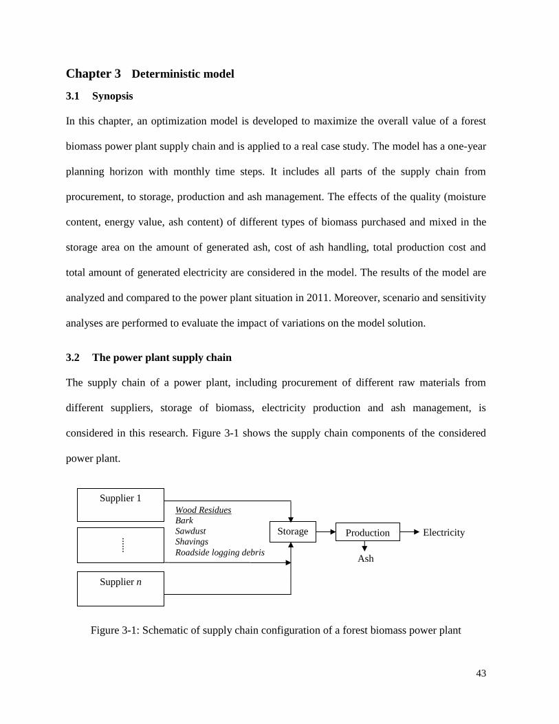
43
Chapter 3 Deterministic model
3.1 Synopsis
In this chapter, an optimization model is developed to maximize the overall value of a forest
biomass power plant supply chain and is applied to a real case study. The model has a one-year
planning horizon with monthly time steps. It includes all parts of the supply chain from
procurement, to storage, production and ash management. The effects of the quality (moisture
content, energy value, ash content) of different types of biomass purchased and mixed in the
storage area on the amount of generated ash, cost of ash handling, total production cost and
total amount of generated electricity are considered in the model. The results of the model are
analyzed and compared to the power plant situation in 2011. Moreover, scenario and sensitivity
analyses are performed to evaluate the impact of variations on the model solution.
3.2 The power plant supply chain
The supply chain of a power plant, including procurement of different raw materials from
different suppliers, storage of biomass, electricity production and ash management, is
considered in this research. Figure 3-1 shows the supply chain components of the considered
power plant.
Figure 3-1: Schematic of supply chain configuration of a forest biomass power plant
Wood Residues
Bark
Sawdust
Shavings
Roadside logging debris
Storage Production
Ash
Electricity
Supplier 1
Supplier n
......

44
Details of each component are explained below.
Raw materials: The forest biomass can be supplied from forest residues, by-products of forest
product mills, or fast growing crops grown specifically for energy purposes (Demirbaş, 2001).
Forest residues include branches and tops left in the harvest areas after the logs have been
transported to wood manufacturing facilities, as well as small diameter and infected trees not
suitable for lumber production. By-products of forest product mills include wood chips,
sawdust, bark and shavings (Demirbaş, 2001). Poplar and willow are examples of fast growing
tree-crops grown specifically for energy purposes (Rockwood et al., 2004).
In addition to the long term availability of biomass, its quality is an important factor in
economic feasibility of bioenergy projects and the amount of energy generated from it. The
quality of biomass depends on a variety of factors such as Higher Heating Value (HHV),
moisture content, physical, chemical and thermal properties. HHV is the amount of heat
released from complete combustion of dry biomass under standard conditions. Different types
of biomass (e.g. bark, sawdust, shavings, etc.) and different species have different HHV’s. The
moisture content affects the biomass heat content since energy has to be used to evaporate
water at the beginning of the combustion process (Saidur et al., 2011). Density, porosity, size
and shape of biomass are other important physical properties of biomass that impact its
utilization as fuel (Saidur et al., 2011). Different energy conversion technologies require
different particle size ranges. For combustion, the particle size of biomass should be between
0.6 cm (Demirbaş, 2005) and 10 cm (Personal communication with power plant managers).
Size and shape can be modified and improved through pre-processing operations such as
chipping which can take place in the forest, a sort yard or at the power plant. Bark, sawdust and
shavings usually need minor screening and chipping, while larger sized raw materials, such as

45
roadside logging debris, need to be chipped before they can be used in direct combustion.
Biomass chemical properties include the ratio of chemical elements, such as carbon, hydrogen,
oxygen, nitrogen, in biomass and its structural components, which is the amount of cellulose,
lignin and hemicelluloses. These properties are different in different species and impact the
HHV of the biomass as mentioned earlier. However, the impact of chemical composition on
combustion is less significant compared to moisture content (Demirbaş, 2007). Important
thermal properties are specific heat, thermal conductivity, and emissivity and vary with the
moisture content and temperature (Saidur et al. (2011), Lehtikangas (2001), Demirbaş (2003),
Demirbaş (2005)).
Transportation: Different transportation modes, e.g. trucks, railcars, vessels and barge, can be
used for transporting biomass to the power plant. However, forest biomass power plants are
usually supplied from local suppliers and therefore road transport is more likely to be used
among other possible methods. As forest biomass density is relatively low (400 and 900 kg/m3
(Demirbaş, 2001)), its transportation to the power plant requires a large number of trucks
which increases the delivered cost of biomass and the complexity of its logistics system.
Biomass can be transported directly to the power plants, or stored at a satellite storage facility
and used later. The transportation cost of biomass depends on the power plant size, raw
material availability, average transportation distance, biomass density, carrying capacity, and
the travelling speed. Transportation and handling costs usually represent a significant
proportion of the total biomass delivered cost (as high as 50% in some cases (Allen et al.,
1998)).
Storage: Storage is an important issue in a forest biomass supply chain. The storage site can be
located either in the forest, at the power station or at an intermediate point. Usually, when

46
forest biomass is kept in a pile, it generates internal heat over time which is the result of
respiration of living cells in wood (Fuller, 1985). The internal heat generated during storage
makes the biomass more homogenous and warmer which makes it burns more easily. Thus, to
improve the quality of biomass, it is better to keep it in storage for a period of time (1-2
months) (Personal communication with power plant managers) and not to let the amount of
biomass in storage drop below a certain level. The storage level has to be kept within certain
limits, which depend on the size of power plant. However, if the storage amount is higher than
a certain level, its handling cost increases incrementally since there is a need for an extra
operator and material handling equipment. The risk of fire and biomass deterioration are also
higher when it is kept in large piles (Fuller, 1985).
Combustion: Direct combustion is a way to convert the energy embedded in biomass and
derived from the sun and stored in biomass through photosynthesis into other forms of energy,
mainly heat and then electricity (Demirbaş, 2001). Combustion is defined as “a series of
chemical reactions resulting in carbon and hydrogen deoxidization” (Demirbaş, 2005).
Biomass elements, moisture content, and air are critical components of wood combustion. The
products of these reactions include CO, hydrocarbons, oxides of nitrogen, sulfur and inorganic
species such as the alkali chlorides, sulfates, carbonates and silicates (Saidur et al., 2011).
When wood is combusted, mass losses occur which is related to the combustion temperature.
This can be depicted in a plot, called the burning profile, which shows the rate of weight loss
against temperature. The first peak in the burning profile is related to the release of moisture
content and a small amount of other absorbed gases. Then, as the temperature increases to
175°-225°, other volatiles chemicals start to be released and ignite. Then, the rate of mass
losses increases drastically up to temperatures between 325° and 425°, when the mass losses

47
start to decrease. This decline will continue and eventually the weight will be almost constant.
These temperatures are different for different types of biomass (Saidur et al., 2011).
Production: The electricity production process depends on the technology used and the layout
of the power plant (Rentizelas et al., 2009b). There are different biomass combustion
technologies for energy generation such as fixed bed combustion, fluidized bed combustion
and pulverized bed combustion (Saidur et al., 2011). The scale of forest biomass energy
conversion plants can vary from very small scale (for domestic heating) up to a scale in the
range of 100 MWe1. The main restriction on the power plant size is the availability of the local
feedstock, which makes it difficult to have biomass power plants larger than 25 MW. If
dedicated feedstock supplies are available, larger power plants can be built producing 50–75
MW. The net electrical efficiency depends on the scale of the power plant and ranges from
20% to 40%. Small sized biomass power plants have low efficiencies, while the large sized
biomass power plants can be as efficient as fossil fuel systems, however, access to high volume
of biomass throughout the year and high cost of transporting low density material are the issues
with these types of plants (Demirbaş, 2001).
In this study, the overall configuration of the forest biomass power plant is based on a
conventional power cycle used in typical thermal utility plants. The power plant uses forest
biomass which is transferred by conveyors to a boiler where it is burned to generate heat for
steam production. The steam is then transferred into a turbine, where the thermal energy is
converted to electrical power. The exhaust steam is converted to water by a condenser and used
in the system again. The water is re-used for almost seven cycles and then it is discharged to
the sewer network. Other equipment pieces might include a high voltage step up transformer, a
1 Megawatt Electrical

48
solid fuel handling system, an ash removal/handling system and other steam cycle auxiliary
pieces of equipment, multiple cyclones and an electrostatic precipitator.
Ash management: Ash management is an important task in a direct combustion power plant.
Generally, wood ash properties are related to several factors such as: species of tree or shrub,
part of the tree or shrub (bark, wood, and leaves), type of waste (wood, pulp, or paper residue),
combination with other fuel sources, type and quality of soil, weather conditions and
combustion process (Saidur et al., 2011). Forest biomass ash generally contains calcium (Ca)
and potassium (K) (Saidur et al., 2011). Two kinds of ash are generated in the production
process: one is derived from soil and rock contamination (called bottom ash) and the other one
is derived from the minerals in the foliage or wood (called fly ash). Ash disposal is a challenge
for most of the power plants and has economic, environmental and social costs for the power
plant. High ash content biomass is less desirable as a fuel (Demirbaş, 2005). For example,
sawdust has lower ash content than bark and logging residues (Lehtikangas, 2001).
In order to design and manage an efficient supply chain for biomass power plants, all of the
above mentioned components of the supply chain should be considered. It is important that the
power plant receives the required amount of biomass at the right time with a competitive price
to meet the electricity demand and maximize the profit. This can be determined by an
optimization model. An optimum configuration of all processes in the supply chain can help
decision makers run a better operation. The optimality is usually related to cost/profit, however
other factors, such as fuel consumption, greenhouse gas emissions and customer satisfaction,
are also important in the supply chain management. Usually there is a trade-off between these
different objectives, which adds its own challenges to the model.

49
3.3 The optimization model
The model presented here considers multiple procurement sources, several storage options,
different types of forest fuel, and several time periods. The overall objective of the
optimization model developed in this study is to provide estimates of the amount of biomass to
be purchased, stored and consumed in each month during a one-year planning horizon. Here,
the main component of the model, decision variables, constraints and the objective function are
defined. Table 3-1 shows the notation and definition of different sets and decision variables
used in the developed model.
Table 3-1: List of indices and decision variables used in the optimization model
Indices
Product type p∈{Bark, Sawdust, Shavings, Roadside Logging Debris (RLD)}
Supplier s ∈ { Supplier1, ..., Supplier8}
Time steps t ∈ {Jan, Feb, ..., Dec}
Decision Variables
Average energy value of the mix of biomass in storage in month t (MW/green tonnes)
Amount of mixed biomass consumed in month t to produce electricity (green tonnes)
Amount of electricity generated in month t (MWh)
Amount of biomass purchased from supplier s in month t (green tonnes)
Amount of mixed biomass stored in month t (green tonnes)
Binary variable, 1 if storage is higher than the storage upper limit (SUL) in month t
Binary variable, 1 if storage is less than the storage lower limit (SLL) in month t
Table 3-2 shows the notation and definition of different sets and decision variables and
parameters used in the developed model.

50
Table 3-2: List of parameters used in the optimization model
Model Parameters
Average ash content of mix of biomass (%)
Cost of ash handling ($/green tonnes)
Unit cost of biomass type p produced at supplier s ($/green tonnes)
Incremental cost of chemical used for power production ($/MWh)
Electricity demand from client in month t (MWh)
ys em’s overall efficie cy (%)
Electricity price in month t ($/MWh)
Energy value of biomass type p purchased from supplier s in month t (MWh/green
tonnes)
Higher heating value of biomass type p purchased from supplier s in month t (MWh/dry
tonnes)
Maximum biomass available from supplier s in month t (green tonnes)
Maximum absolute storage capacity (green tonnes)
Moisture content of biomass type p purchased from supplier in month t (%)
Penalty cost if storage is above the storage upper limit ($)
The percentage of reduction in biomass quality if storage level is below SLL
The ratio of biomass type p produced at supplier s in month t (%)
Incremental cost of sewer used for power production ($/MWh)
Storage lower limit. If the storage level is below this level, the biomass quality decreases
since there is not enough time for it to be mixed and produce internal heat (green tonnes)
Storage upper limit (green tonnes)
Target storage for the last month (green tonnes)
Biomass transportation cost for supplier s in month ($/green tonnes)
Incremental cost of water used for power production ($/MWh)
The objective function is to maximize the profit (Equation 3.1).
(3.1)

51
Revenue from selling electricity to customer(s) is calculated by multiplying the electricity unit
price by the amount of electricity produced by the power plant (Equation 3.2).
∑ (3.2)
Biomass procurement costs include the cost of purchasing biomass and its transportation costs
(Equation 3.3). The biomass purchase cost is calculated by multiplying the biomass price by
the ratio of each biomass type produced in each supplier and the amount of biomass purchased.
The transportation costs depend on the distance between suppliers and the power plant, and the
amount of purchased biomass. It is assumed that no chipping is done in this power plant. If this
is not the case, the model can easily be modified to include that.
∑ ∑ (3.3)
Ash handling cost is equal to the average ash content of all biomass multiplied by the amount
of biomass consumed for power production multiplied by the cost of handling ash (Equation
3.4). It should be noted that the average ash content is considered in this equation which can be
substituted by more detailed parameter such as ash content of each type of biomass if enough
data were available. Usually different types of wood are burnt together; therefore, the ash
content of the mix of biomass is available.
∑ (3.4)
The penalty storage cost is calculated by multiplying a fixed penalty cost by a binary variable if
the decision variable related to storage is more than a certain level (SUL) (Equation 3.5).
∑ (3.5)

52
The production cost contains water, sewer and chemical costs multiplied by the amount of
power produced by the power plant (Equation 3.6).
∑ (3.6)
Constraints of the model are listed below:
In month t, biomass purchased from supplier s has to be less than or equal to the maximum
biomass produced by that supplier.
[For all s, t] (3.7)
Storage level in each month has to be less than or equal to the absolute maximum storage
levels.
[For all t] (3.8)
Equation 3.9 implies the storage in the final month of the year has to be equal to a target
storage level. This constraint guarantees a desired initial storage condition for the next year that
can be set by managers.
(3.9)
Mass balance equation is considered in Equation 3.10, which indicates that storage in month
is equal to storage in month (t-1) plus the total biomass purchased from all suppliers minus
biomass consumption in month t.
∑ [For all t] (3.10)

53
Equation 3.11 shows that the power generated by the power plant in each month has to be
equal o he cus omer’s mo hly dema d.
[For all t] (3.11)
Equation 3.12 relates the amount of electricity produced in each month to the energy value of
biomass utilized in that month, efficiency of the system and the reduction in biomass quality if
the storage level is less than the SLL (1-QRF×Zt).
[For all t] (3.12)
The average energy value of biomass in storage in month t is calculated based on the weighted
average of energy values of biomass purchased from suppliers in that month and the average
energy value of stored biomass in month (t-1) as shown in Equation 3.13.
∑ ∑
∑
[For all t] (3.13)
AveEVt is a decision variable since it is calculated based on variables Fs,t and St-1. EVs,p,t is
calculated based on higher heating value HHVs,p,t and the corresponding moisture content
MCs,p,t of biomass as implied in Equation 3.14 (Bowyer et al., 2007).
[For all s, p, t] (3.14)
And finally, all the continuous variables are non-negative as shown in Equation 3.15.
[for all t] (3.15)

54
When the model is formulated, additional constraints have to be added for definition of binary
variables Yt and Zt. Yt is defined as:
{
(3.16)
The following constraints (Equations 3.17 and 3.18) are equivalent to the above definition and
replaced it in the model formulation, where M is a sufficiently large number.
[For all t] (3.17)
[For all t] (3.18)
The same constraints have to be added to the model for Zt. Zt is defined as:
{
(3.19)
It can be seen that the model is a nonlinear mixed integer programming (MINLP) model since
Equations 3.12 and 3.13 contain non-linear terms and the model contains both continuous and
binary variables.
MINLP is a combination of two theoretically difficult to solve categories of problems
particularly for large scale problems: mixed integer programs (MIP) and nonlinear programs
(NLP). Therefore, it is not straightforward to solve MINLP problems and get precise results
(Bussieck & Pruessner, 2003). However, several methods have been developed and improved
in the past few years which make it possible to solve MINLP problems more precisely under
special circumstances (convexity, etc.), i.e. terminate with a guaranteed optimal solution or

55
prove that no such solution exists (Bonami & Gonçalves, 2012). The solution methods include
branch-and-bound method (Dakin, 1965), Benders decomposition (Geoffrion, 1972) and Outer
Approximation (OA) algorithm (Duran & Grossmann, 1986).
In this study, the Outer Approximation (OA) algorithm was used since it was provided in the
AIMMS software package (AIMMS. Paragon Decision Technology). The idea in this
algorithm is to switch between solving the nonlinear programming sub-problems and the
relaxed versions of a mixed integer linear master program for a finite sequence. The main
assumption in the Outer Approximation algorithm is the convexity of the nonlinear sub-model.
3.4 Case study
The above model was applied to a case study located in Canada to help maximize profit and
manage supply chain efficiently. The supply chain is the same as what was described in section
3.3. Most of the biomass used by the power plant was supplied from residues from local
sawmills at a low cost. These inexpensive sources of raw material started to decline in recent
years due to the economic downturn that resulted in the closure of some of the mills in the area,
and the competition for biomass from pellet mills. Therefore, biomass prices have increased
and the power plant was forced to use other sources of biomass such as logging debris.
Biomass from different sources has different quality and cost which affect the costs and
efficiency of the operation.
Table 3-3 shows some of the characteristics of the power plant.

56
Table 3-3: Characteristics of the case study
Number of suppliers with a fixed (long term) contract 4
Number of suppliers without a fixed contract More than 50 suppliers
Average ash content 8%
Average moisture content (MC) 32.4% (range: 10.2-46.7)
Average higher heating value (HHV) 5.53 MWh/tonnes (range: 4.06-
5.89)
8565 BTU/lb (range: 6275-9110)
Efficiency 30%
Range of available biomass from suppliers with a fixed contract 0-12,861 (green tonnes per month)
Range of available biomass from suppliers without a fixed
contract
0-18,900 (green tonnes per month)
Some of the specifications of the case study supply chain are presented below.
Raw material: The feedstock used in the power plant includes bark, sawdust, shavings and
roadside logging debris (RLD):
∈
All types of biomass are transported to the power plant by trucks and then kept in storage and
mixed together before combustion. There is a long list of possible suppliers for the power plant
with different contracts, terms, conditions and prices. For some suppliers, if they are in the
operation, the power plant has to buy their biomass. These mills are located close to the power
plant and their biomass is relatively inexpensive because of the short transportation distance
and long term contracts. However, if these mills decide not to operate, there will be a raw
material shortage for the power plant. Therefore, the amount of biomass that can be purchased
from these suppliers is not exactly known in advance. There are other suppliers which can be
considered as ad-hoc suppliers which have no contract with the power plant and usually

57
provide more expensive biomass. Therefore, Equation 3.7 can be broken into two sets of
constraints:
[For all s in suppliers with a fixed contract, t] (3.20)
[For all s in suppliers without a fixed contract, t] (3.21)
Storage: The capacity of the storage for biomass is limited and known. Storing more than a
certain level of biomass forces the power plant to hire an additional operator and use additional
material handling equipment. In addition, there is another upper storage limit, above which
additional operator and additional handling material equipment are needed, and the risk of fire
in the storage facility increases. Therefore, in the model if storage is more than the first upper
level in month t, a binary variable called Xt becomes 1 and if it is more than the second upper
storage level, another binary variable called Yt becomes also 1. Then, the storage penalty cost
will be:
∑ (3.22)
If the level of the storage decreases below a certain level called the minimum storage level, the
quality of biomass is decreased by a certain amount (6% in this case) and there is a risk of
biomass shortage (Equation 3.12).
Demand: The power plant has a long term contract with a customer to provide a fixed amount
of electricity per year, called the firm load. The rest of the production, named the surplus load,
can be produced and sold to the same customer whenever it is profitable. The firm load demand
has to be met at all times, while the power plant has the option to not produce the surplus load.

58
There is also a total amount for the firm load demand in a year. Usually, the power plant
decides whether or not to produce the surplus load in the beginning of the year and informs the
customer about its decision. If the power plant decides to produce the surplus load, the first
fixed amount of production in each hour is considered as the firm load and the rest is the
surplus load. When the production covers the firm demand, the rest of the production is
considered as the surplus demand. If the power plant decides to not produce the surplus load,
the total production in each hour is considered as the firm load and the power plant will be shut
down for the rest of the year after meeting the total firm demand.
To model different demand types, several parameters and decision variables have to be added
explained in Table 3-4.
Table 3-4: Variables and parameters of the case study
Symbol Type Definition
Continuous Variable Total electricity generated in each month (MWh)
Binary Variable 1 if surplus electricity is produced in a year, 0 otherwise
Parameter Energy price for firm load ($/MWh)
Parameter Total firm demand in one year (MWh)
Parameter Amount of firm electricity generated in month t if the surplus is
not being produced (MWh)
Parameter Total surplus demand in one year (MWh)
Parameter Energy price for surplus load ($/MWh)
Parameter Number of working hours in month t
Then, the following constraint (Equation 3.23) needs to be added to the model. This constraint
implies that the electricity produced in each month has two forms. If the surplus load is being
produced, it is equal to the total firm and surplus demand in one year distributed monthly based
on the ratio of working hours of that month to the total working hours in one year. If the

59
surplus load is not being produced, the electricity demand in each month is equal to the firm
load generated in each month.
∑ (3.23)
The objective function also needs to be modified since the revenue from selling electricity to
the customer is equal to the firm load demand multiplied by the power price for the firm load
plus the surplus load demand multiplied by the surplus energy price multiplied by the binary
variable if the surplus power is being produced.
(3.24)
The optimization model for this case study includes Equations 3.8, 3.9, 3.10, 3.11, 3.12, 3.13,
3.15, 3.17, 3.18, 3.20, 3.21 and 3.23 (and corresponding constraints for definition of Zt) and the
objective function is to maximize (3.24 – 3.3 – 3.4 – 3.6 – 3.22).
The MINLP model was solved using the AIMMS software (AIMMS. Paragon Decision
Technology) and the Outer Approximation algorithm. The model had 260 variables (73 binary
variables and 187 continuous variables) and 333 constraints. It took less than a minute to solve
the problem using a 2.80 GHz CPU. The model was implemented with real data and validated
by the power plant managers. It is notable that this model can be used for monthly decision
making. It means that the model can be used at the beginning of the planning horizon (Jan) to
indicate the optimal decision variables. However, if some parameters change later, the model
can be updated using the new information, the previous month’s variables have to be fixed
based on the real values and the model can be run again for the rest of the months.
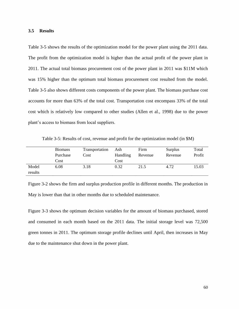
60
3.5 Results
Table 3-5 shows the results of the optimization model for the power plant using the 2011 data.
The profit from the optimization model is higher than the actual profit of the power plant in
2011. The actual total biomass procurement cost of the power plant in 2011 was $11M which
was 15% higher than the optimum total biomass procurement cost resulted from the model.
Table 3-5 also shows different costs components of the power plant. The biomass purchase cost
accounts for more than 63% of the total cost. Transportation cost encompass 33% of the total
cost which is relatively low compared to other studies (Allen et al., 1998) due to the power
pla ’s access o biomass from local suppliers.
Table 3-5: Results of cost, revenue and profit for the optimization model (in $M)
Biomass
Purchase
Cost
Transportation
Cost
Ash
Handling
Cost
Firm
Revenue
Surplus
Revenue
Total
Profit
Model
results
6.08 3.18 0.32 21.5 4.72 15.03
Figure 3-2 shows the firm and surplus production profile in different months. The production in
May is lower than that in other months due to scheduled maintenance.
Figure 3-3 shows the optimum decision variables for the amount of biomass purchased, stored
and consumed in each month based on the 2011 data. The initial storage level was 72,500
green tonnes in 2011. The optimum storage profile declines until April, then increases in May
due to the maintenance shut down in the power plant.
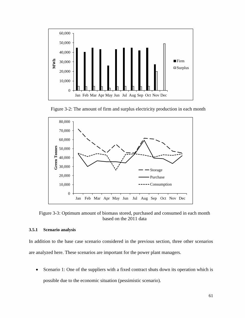
61
Figure 3-2: The amount of firm and surplus electricity production in each month
Figure 3-3: Optimum amount of biomass stored, purchased and consumed in each month
based on the 2011 data
3.5.1 Scenario analysis
In addition to the base case scenario considered in the previous section, three other scenarios
are analyzed here. These scenarios are important for the power plant managers.
Scenario 1: One of the suppliers with a fixed contract shuts down its operation which is
possible due to the economic situation (pessimistic scenario).
0
10,000
20,000
30,000
40,000
50,000
60,000
Jan Feb Mar Apr May Jun Jul Aug Sep Oct Nov Dec
MW
h
Firm
Surplus
0
10,000
20,000
30,000
40,000
50,000
60,000
70,000
80,000
Jan Feb Mar Apr May Jun Jul Aug Sep Oct Nov Dec
Gre
en T
on
nes
Storage
Purchase
Consumption

62
Scenario 2: One of the previous suppliers with a fixed contract which was closed in the
past couple of years resumes its operation (optimistic scenario).
Scenario 3: The power plant makes an investment in a new piece of equipment for ash
recovery. Having a new ash recovery system with a capital cost of $2M, the ash
generated in the power plant is screened and the unburnt parts are separated and sent
back to the operation process. It has been estimated that this system will collect 20% of
the ash and use it as a biomass source. It is assumed that the energy value of the unburnt
part of the ash is the same as the average energy value of the biomass consumed in that
month. Therefore, it has the potential benefit of providing more biomass and less ash
for the power plant which reduces the ash disposal costs.
Table 3-6 shows the total profit and the total purchase cost of biomass for different scenarios.
The results show that Scenario 1 has a lower profit (24.48%) than the base case scenario.
Scenario 2 has a higher profit than the base case scenario since the power plant has access to
cheaper biomass from a supplier with a fixed contract. The amount of increase in profit is
$3.27M (21.76%) which is the result of reduction in the biomass purchase cost. Scenario 3,
investment in a new ash recovery system, has a higher profit than the base case scenario
($160,000, 1.06%). This means that investing in a new ash recovery system has economic and
environmental benefits for the power plant. The increase in profit is partly from the reduction
in the biomass purchase cost (3.46%), and partly from reduction in the ash handling cost
(20.75%). The capital cost of the ash recovery equipment was converted to the yearly cost
using a 2% interest rate and 10 years’ service life, and then the yearly cost was subtracted from
the profit.

63
Table 3-6: Total profit and biomass procurement cost for four different scenarios
Base Case Scenario Scenario 1 Scenario 2 Scenario 3
Total Profit ($M) 15.03 11.35 18.30 15.19
Biomass Procurement Cost ($M) 9.26 12.94 6.00 8.94
Profit difference compared to the base
case scenario
0 -24.48% +21.76% +1.06%
3.5.2 Sensitivity analysis
To evaluate the effect of variations in model parameters on the profit, sensitivity analysis was
performed. The results of variation in profit are depicted in Figure 3-4. It can be seen that the
impact of variation in some of the parameters, such as electricity price, higher heating value
and maximum available biomass from suppliers with a fixed contract have a large impact on
the profit. When these parameters increase by 20%, the increase in profit is between 20-35%.
On the other hand, when they are reduced by 20%, the loss is 23-45%. Other parameters are:
moisture content, biomass cost and transportation costs which have the opposite impact on the
profit. Increasing these parameters by 20%, decreases the profit by about 4-15%. The effects
of variation in other parameters on the overall profit are low and can be considered negligible.
The sensitivity of the results to changes in initial storage level was also determined. The initial
storage level was changed from 0 to 118,000 green tonnes, while the target storage level was
set to the initial storage level. As shown in Figure 3-5, an initial storage level of 109,000 green
tonnes generates the highest profit.

64
Figure 3-4: Variations in profit with 20% change in different parameters
Figure 3-5: Variations in profit for different initial storage levels
-50%
-40%
-30%
-20%
-10%
0%
10%
20%
30%
40%
-30% -20% -10% 0% 10% 20% 30%
Pro
fit
Dif
fere
nce
Change in Parameter
Max biomass from supplier
with fixed contract
Max biomass from supplier
without fixed contract
Ash content
Electricity price
Quality reduction factor
HHV
MC
Transportation cost
Wood cost
0
2
4
6
8
10
12
14
16
0 20,000 40,000 60,000 80,000 100,000 120,000 140,000
Pro
fit
($M
)
Initial Storage (Green Tonnes)

65
3.6 Discussion and conclusions
In this chapter, a mathematical optimization model was developed to determine the amount of
biomass to purchase from each supplier in each month, the amount of mixed biomass to burn
and store in each month, and whether or not to produce extra electricity to maximize the total
profit. The developed model was a mixed integer non-linear model, which was solved by the
Outer Approximation algorithm using the AIMMS software package. The results for the
specific case study presented here indicated that the profit from the optimization model was
higher than that of the actual profit generated by the power plant in 2011 when he compa y’s
managers made decisions based on their experience. For instance, the optimum biomass
procurement cost was $9.26M, which was 15% lower than the actual purchase and
transportation costs of the power plant in 2011 ($11M). The model provided the optimum
profile for biomass storage, purchase and consumption in each month to achieve maximum
profit over a year. The model could be re-optimized and updated if input data varied from what
had been used here.
The power plant situation in 2011 was considered as the base case scenario and three other
scenarios were evaluated in this study. The first one was a pessimistic scenario in which the
production shutdown of a supplier with a fixed contract was investigated. The second scenario,
an optimistic scenario, was related to the resumption of production at one of the previous
suppliers with a fixed contract. And finally, the third scenario investigated the investment in a
new ash recovery system. This system collects and reuses the unburnt parts of the produced
ash. Based on the results, the profit of the first scenario was 24% lower than that of the base
case scenario, while the profit of second and third scenarios were 22% and 1% higher than that

66
of the base case scenario, respectively. The reason for having lower profit in the first scenario
is that the power plant had no longer access to one of its supplier (located in the area and
providing inexpensive biomass). Therefore, it needed to purchase more expensive biomass
from ad-hoc suppliers. For the second scenario, it was other way around, meaning that an extra
inexpensive source of biomass with a fixed long term contract was available for the power
plant. Therefore, it resulted in having a higher profit than the base case scenario. In the third
scenario, the ash handling cost reduced by 21%. Therefore, investing in a new ash recovery
system could have economic benefit as well as environmental advantage for the power plant.
This chapter addressed the first, second and part of the third objectives mentioned in 1.2. It
provided an integrated framework for optimizing the supply chain of a forest biomass power
plant. The developed model was then applied to a real case study. The model and its results
were validated by the power plant managers. It was a mixed integer non-linear programming
model with multiple time steps and captured seasonal variations in parameters particularity in
biomass availability and quality. The quality of the mix of material in the storage was
calculated, and the impact of any change in the quality of each biomass type from each supplier
in each month on the solution could be examined. Therefore, it included the issue of quality in
the modeling and provided optimum decisions on biomass purchase, storage and consumption
in order to meet electricity demand in each month.
The impact of changes in input parameters on the profit was determined using sensitivity
analysis. Parameters that had higher impact on the model solution were also identified.
However, uniform changes in input parameters were considered in sensitivity analysis. In other
words, it was assumed that uncertainties in all parameters had the same nature and they could

67
have any value within a defined range with the same probability. This is not a realistic
assumption since there are different sources of uncertainty in the system and some of the
uncertain parameters are correlated with one another. Moreover, not all the possible
realizations of uncertain parameters occur with the same probability. To capture these issues,
Monte Carlo simulation is used to model the uncertainties in input parameters more
realistically, as can be seen in the next chapter.

68
Chapter 4 Monte Carlo simulation
4.1 Synopsis
In this chapter, Monte Carlo simulation is used in combination with the optimization model
developed in Chapter 3 to evaluate the impact of uncertainty in different parameters including
biomass quality, availability and cost and electricity prices based on historical data. Different
types of uncertain parameters are incorporated in the model. Historical data on biomass quality
(moisture content and higher heating value) obtained from the power plant is used to generate
fitted probability distributions. The Monte Carlo simulation and the optimization model
provide a probability distribution for possible optimal solution that can be used for
u ders a di g he sys em’s behaviour i he prese ce of u cer ai y, ide ifyi g he risks a d
opportunities in the supply chain, and making informed decisions.
4.2 Uncertainty and Monte Carlo simulation
Vose (2008) divided the uncertainty based on its origin into two categories: 1) uncertainty
resulted from incomplete understanding of a system due to its complexity, and 2) uncertainty
related to the random nature of a parameter, which was called “variabili y” by he au hor.
Approaches to be used for dealing with uncertainties in the model and actions to be taken in
response to them vary given the source of uncertainty in stochastic parameters. While
collecting more information is effective in expanding the knowledge about a random event,
understanding a system or trying to modify it might be more useful in managing uncertainties
resulting from system complexity. Thus, it is important to evaluate the impacts of these two
types of uncertainty separately to realise the impact of each on the solution. This helps decision

69
makers identify the proper steps to take to mitigate the risks and take advantage of possible
opportunities associated with variations in the system (Vose, 2008).
The results of the sensitivity analysis performed and presented in Chapter 3 showed that
parameters with higher impact on the optimum solution were the monthly available biomass
from each supplier (MaxFs,t), biomass MC and HHV, biomass cost and electricity prices.
Availability and cost of biomass, as well as electricity price can be grouped together because
they are affected by economic and market conditions. Moreover, due to interdependency
between different forest sectors and diverge production structure of industries, variations in one
part of this supply chain can propagate into the other parts. Therefore, availability and cost of
biomass are impacted by variations in other forest product sectors such as lumber and pulp and
paper sectors. On the other hand, uncertainty in biomass quality is related to the heterogeneous
nature of wood resulting from the variations in its physical and chemical characteristics from
different species and different parts of a tree (Bowyer et al., 2012). Biomass quality is also
affected by external factors, such as growth conditions and climate, and can change during
storage, production, and transportation. It impacts collection, transportation, handling, storage
and the efficiency of conversion technology (Rentizelas et al., 2009b).
AIMMS software package (AIMMS. Paragon Decision Technology) was used to model Monte
Carlo simulation along with the optimization model. Monte Carlo simulation is first performed
for each group of the uncertain parameters separately to study their specific impact on the
power pla ’s profi . The , a overall u cer ai y a alysis is co duc ed by allowi g he i pu
parameters to change over their respective probability distributions/ ranges simultaneously. The
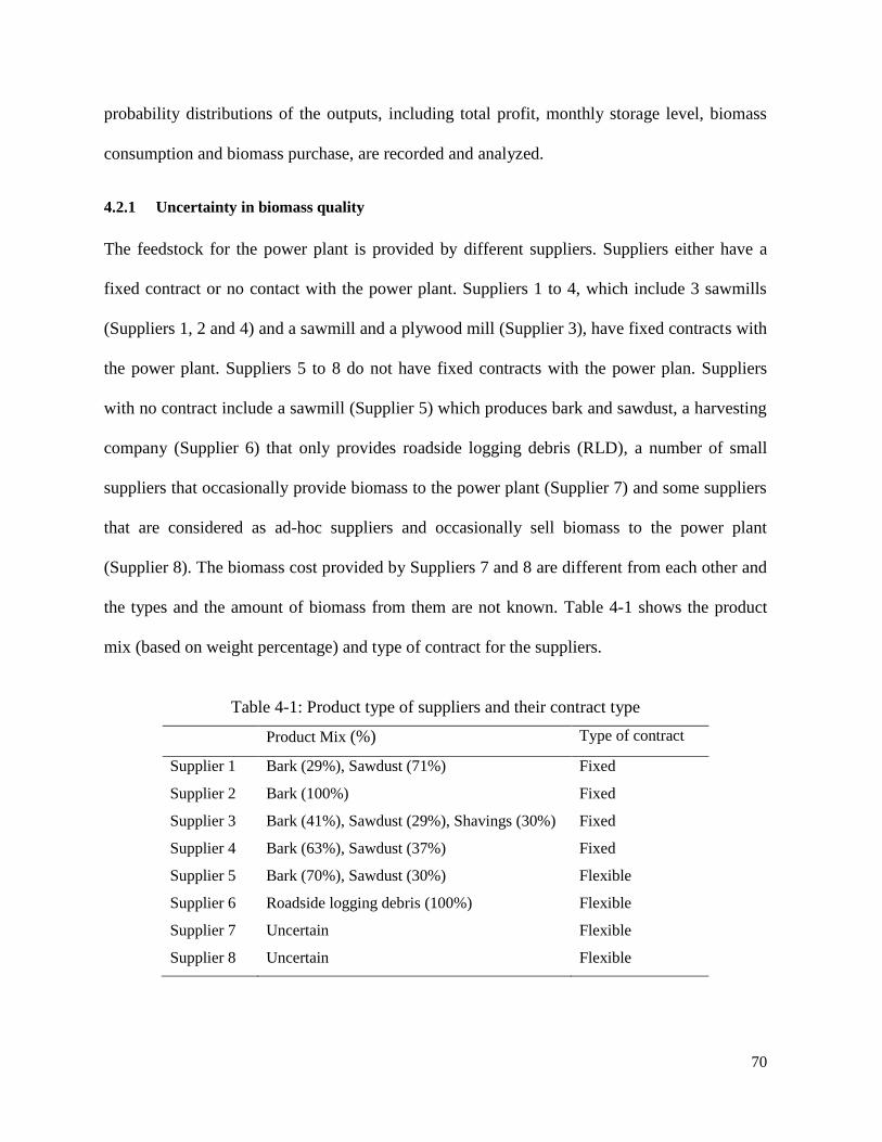
70
probability distributions of the outputs, including total profit, monthly storage level, biomass
consumption and biomass purchase, are recorded and analyzed.
4.2.1 Uncertainty in biomass quality
The feedstock for the power plant is provided by different suppliers. Suppliers either have a
fixed contract or no contact with the power plant. Suppliers 1 to 4, which include 3 sawmills
(Suppliers 1, 2 and 4) and a sawmill and a plywood mill (Supplier 3), have fixed contracts with
the power plant. Suppliers 5 to 8 do not have fixed contracts with the power plan. Suppliers
with no contract include a sawmill (Supplier 5) which produces bark and sawdust, a harvesting
company (Supplier 6) that only provides roadside logging debris (RLD), a number of small
suppliers that occasionally provide biomass to the power plant (Supplier 7) and some suppliers
that are considered as ad-hoc suppliers and occasionally sell biomass to the power plant
(Supplier 8). The biomass cost provided by Suppliers 7 and 8 are different from each other and
the types and the amount of biomass from them are not known. Table 4-1 shows the product
mix (based on weight percentage) and type of contract for the suppliers.
Table 4-1: Product type of suppliers and their contract type
Product Mix (%) Type of contract
Supplier 1 Bark (29%), Sawdust (71%) Fixed
Supplier 2 Bark (100%) Fixed
Supplier 3 Bark (41%), Sawdust (29%), Shavings (30%) Fixed
Supplier 4 Bark (63%), Sawdust (37%) Fixed
Supplier 5 Bark (70%), Sawdust (30%) Flexible
Supplier 6 Roadside logging debris (100%) Flexible
Supplier 7 Uncertain Flexible
Supplier 8 Uncertain Flexible
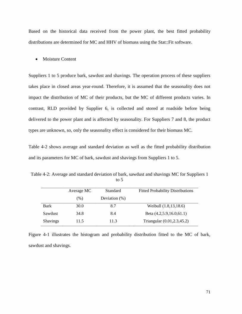
71
Based on the historical data received from the power plant, the best fitted probability
distributions are determined for MC and HHV of biomass using the Stat::Fit software.
Moisture Content
Suppliers 1 to 5 produce bark, sawdust and shavings. The operation process of these suppliers
takes place in closed areas year-round. Therefore, it is assumed that the seasonality does not
impact the distribution of MC of their products, but the MC of different products varies. In
contrast, RLD provided by Supplier 6, is collected and stored at roadside before being
delivered to the power plant and is affected by seasonality. For Suppliers 7 and 8, the product
types are unknown, so, only the seasonality effect is considered for their biomass MC.
Table 4-2 shows average and standard deviation as well as the fitted probability distribution
and its parameters for MC of bark, sawdust and shavings from Suppliers 1 to 5.
Table 4-2: Average and standard deviation of bark, sawdust and shavings MC for Suppliers 1
to 5
Average MC
(%)
Standard
Deviation (%)
Fitted Probability Distributions
Bark 30.0 8.7 Weibull (1.8,13,18.6)
Sawdust 34.8 8.4 Beta (4.2,5.9,16.0,61.1)
Shavings 11.5 11.3 Triangular (0.01,2.3,45.2)
Figure 4-1 illustrates the histogram and probability distribution fitted to the MC of bark,
sawdust and shavings.

72
Figure 4-1: Histogram and probability distribution of MC of bark (a), sawdust (b), shavings (c)
Table 4-3 presents the average and standard deviation as well as the fitted probability
distribution and its parameters for biomass in different months for suppliers 6 (RLD only). It
should be noted that harvesting operation is not done in the area in May so there is no RLD
available for that month.
Figure 4-2 shows the histogram and probability distribution fitted to the MC of RLD in
different months.
a b
c

73
Table 4-3: Average and standard deviation of biomass MC for Supplier 6
Supplier 6 (RLD) Fitted Probability Distributions
Ave MC (%) SD (%)
January 26.6 5.6 Triangular (0.9,13.8,33.5)
February 36.2 8.4 Gamma (2.8,21,5.41)
March 33.7 9.1 Weibull (2.6,10.0,26.4)
April 45.5 16.6 Beta (0.9,0.8,15.0,69.7)
May - - -
June 25.5 10.7 Triangular (0.3,7.3,51.5)
July 23.7 5.6 Weibull (1.3,15.0,9.32)
August 21.1 4.9 Beta (0.8,0.7,12.0,27.4)
September 24.0 5.6 Triangular (0.5,10.3,38.7)
October 27.1 10.1 Weibull (1.5,12.0,16.8)
November 28.5 6.1 Weibull (1.5,19.0,10.4)
December 35.6 7.6 Triangular (0.1,25.3,55.7)
a b

74
c d
e f
g h
i j

75
Figure 4-2: Histogram and probability distribution for MC of RLD in January (a), February (b),
March (c), April (d), June (e), July (f), August (g), September (h), October (i), November (j),
and December (k)
Higher Heating Value
Table 4-4 shows the average, standard deviation, the fitted probability distribution and its
parameters for HHV of different types of biomass received by the power plant from different
suppliers. It was not possible to fit a distribution for the HHV of bark and shavings because of
the low number of data points, therefore, a range was considered for their variations.
Table 4-4: Average and standard deviation of HHV for different biomass types
HHV Average Standard Deviation Fitted Probability Distributions
Bark 8534 BTU/lb2
5.51 MWh/tonnes
670 BTU/lb
0.43 MWh/tonnes
Uniform (7570.0,9110.0) (BTU/lb)
Uniform (4.89,5.89) (MWh/tonnes)
Sawdust 8537 BTU/lb 5.51
MWh/tonnes
325 BTU/lb
0.21 MWh/tonnes
Uniform (8050.0,8960.0) (BTU/lb)
Uniform (5.20,5.79) (MWh/tonnes)
Shavings 8517 BTU/lb 5.50
MWh/tonnes
254 BTU/lb
0.16 MWh/tonnes
Uniform (8360.0,8810.0) (BTU/lb)
Uniform (5.40,5.69) (MWh/tonnes)
RLD 8392 BTU/lb 5.42
MWh/tonnes
347 BTU/lb
0.22 MWh/tonnes
Weibull (6.1,6960.0,1580.0) (BTU/lb)
Weibull (6.19, 4.41,1.089)
(MWh/tonnes)
2 BTU/lb= 0.0006461MWh/tonnes
k

76
Figure 4-3 show the histogram and probability distribution fitted for HHV of bark and RLD.
Figure 4-3: Histogram and probability distribution of HHV of sawdust (a) and RLD (b)
4.2.2 Uncertainty in biomass availability and cost and electricity price
The amount of by-products generated by he power pla ’s suppliers depends on the production
of their main products, which are mainly used in housing construction. In the past few years,
many sawmills in the area were closed due to the real estate meltdown in the US. Thus, the
power plant faced a shortage of raw material. Conversely, when the market is promising, the
sawmills produce a large amount of biomass that the power plant is obliged to buy. The
situation with a supplier without a fixed contract is less critical since there is no obligation for
the power plant to buy their biomass. However, there still exists uncertainty in the available
biomass that they can provide. Moreover, biomass procurement and transportation costs vary
due to the competition for biomass from other sectors, such as the wood pellets sector, and as a
result of variations in fuel cost. Electricity prices are also uncertain and have to be forecasted
ahead of the time so that the power plant can decide about whether or not to produce surplus
demand in the upcoming year.
a b

77
Uncertainty in electricity prices, and biomass availability and cost are considered together
because they are all related to the economic situation and considered to be correlated. Based on
the historical data, three electricity price scenarios (high, medium and low) with their
corresponding annual available biomass from different suppliers were selected. The annual
available biomass was then distributed over a year based on the monthly production profile of
2011. The Monte Carlo simulation model was run for each scenario with ±20% variation in
monthly biomass availability and ±10% variation in biomass cost.
4.3 Results
The number of iterations for Monte Carlo simulation depends on the desired accuracy and
confidence levels, and is calculated using Equation 4.1 (You et al., 2009):
where N is the number of iterations, Z is the confidence interval of a two tailed normal
distribution, σ is he model’s ou pu s a dard devia io a d εμ is the desired marginal
error. Based on the marginal error of 6%, confidence level of 95% (Z=1.96), and standard
deviation of model results for 100 runs, the required number of iterations was estimated to be
1000.
Table 4-5 shows mean, minimum, maximum and standard deviation of profit and the feasibility
rate obtained from the output of the Monte Carlo simulation-optimization model when MC and
HHV were generated separately from their probability distributions. It can be seen that
incorporating the variability in MC resulted in higher average and standard deviation for the
profit compared to that of HHV. Variability in HHV changes the profit within a $280,000

78
interval with an average of $15.1M, while for MC, the variation in the profit is $700,000 with
an average of $15.3M as shown in Figure 4-4 and Figure 4-5.
Table 4-5: Minimum, maximum, average and standard deviation of profit for considering
uncertainty in different parameters
Uncertain
Parameter
Mean, (Min, Max) of
Profit ($M)
Standard Deviation
($M)
Feasibility
Rate
MC 15.3 (14.1-16.5) 0.35 (2%) 99.9%
HHV 15.1 (14.6-15.6) 0.14 (1%) 99.9%
Figure 4-4: Histogram of profit when MC varies
Figure 4-5: Histogram of profit when HHV varies
0%
5%
10%
15%
20%
25%
30%
14.1
0-1
4.1
9
14.2
0-1
4.2
9
14.3
0-1
4.3
9
14.4
0-1
4.4
9
14.5
0-1
4.5
9
14.6
0-1
4.6
9
14.7
0-1
4.7
9
14.8
0-1
4.8
9
14.9
0-1
4.9
9
15.0
0-1
5.0
9
15.1
0-1
5.1
9
15.2
0-1
5.2
9
15.3
0-1
5.3
9
15.4
0-1
5.4
9
15.5
0-1
5.5
9
15.6
0-1
5.6
9
15.7
0-1
5.7
9
15.8
0-1
5.8
9
15.9
0-1
5.9
9
16.0
0-1
6.0
9
16.1
0-1
6.1
9
16.2
0-1
6.2
9
16.3
0-1
6.3
9
16.4
0-1
6.4
9
Fre
quen
cy
Profit ($M)
0%
5%
10%
15%
20%
25%
30%
14.6
0-1
4.6
9
14.7
0-1
4.7
9
14.8
0-1
4.8
9
14.9
0-1
4.9
9
15.0
0-1
5.0
9
15.1
0-1
5.1
9
15.2
0-1
5.2
9
15.3
0-1
5.3
9
15.4
0-1
5.4
9
15.5
0-1
5.5
9
Fre
quen
cy
Profit ($M)

79
As explained before, three scenarios were considered for electricity price and biomass
availability and cost. The results of the Monte Carlo simulation-optimization model for the
three scenarios are shown in Table 4-6.
Table 4-6: Results of Monte Carlo simulation-optimization model for scenarios of electricity
price and biomass availability and cost
Scenario Surplus Electricity Price
($/MWh)
Mean Profit ($M) SD ($M) Feasibility rate
(%)
Low 35.00 14.4 0.1 100
Average 42.50 15.1 0.5 99.9
High 103.87 17.6 0.2 99.3
Figure 4-6 represents the profit histogram when availability and prices vary together for low,
average and high electricity price scenarios. It can be seen that despite the low standard
deviation of low electricity price scenario, its profit histogram is more bell-shaped, while the
histogram of profit for average and high electricity price scenario are more skewed to higher
profit ranges.
0%
10%
20%
30%
40%
50%
60%
70%
14.3
0-1
4.3
9
14.4
0-1
4.4
9
14.5
0-1
4.5
9
14.6
0-1
4.6
9
14.7
0-1
4.7
9
14.8
0-1
4.8
9
14.9
0-1
4.9
9
15.0
0-1
5.0
9
Fre
quen
cy
Profit ($M) a
0%
10%
20%
30%
40%
50%
60%
70%
13.8
0-1
3.8
9
13.9
0-1
3.9
9
14.0
0-1
4.0
9
14.1
0-1
4.1
9
14.2
0-1
4.2
9
14.3
0-1
4.3
9
14.4
0-1
4.4
9
14.5
0-1
4.5
9
14.6
0-1
4.6
9
14.7
0-1
4.7
9
14.8
0-1
4.8
9
14.9
0-1
4.9
9
15.0
0-1
5.0
9
15.1
0-1
5.1
9
15.2
0-1
5.2
9
15.3
0-1
5.3
9
15.4
0-1
5.4
9
Fre
quen
cy
Profit ($M) b

80
Figure 4-6: Histogram of profit when electricity price and biomass availability and cost vary
for a) low, b) average and c) high scenarios
Table 4-7 provides the probability of having profit within a certain range obtained from the
Monte Carlo simulation-optimization model. The last row represents the results for the case
that uncertainty is included in all parameters. The risk of having profit less than $14M for the
low electricity price scenario is 99%. For the average electricity price scenario, it is more likely
to have profit between $14M and $15M, while in the high electricity price scenario the profit is
always more than $17M. When variation and uncertainty in all parameters are considered, the
risk of having a profit less than $14M is 6%, while there is 32% chance of having a profit
higher than $17M. Most of the time (62%), the compa y’s profi is be wee $14M a d $16M.
Because variations in biomass cost and availability and electricity prices affect the profit of the
power plant significantly and increase the risk of having low profits when electricity prices are
low, the power plant managers should pay special attention to the contract details with
suppliers and forecast of electricity prices.
The outputs of the Monte Carlo simulation-optimization model show that in order to have a
profit higher than $15.5M, the average MC should be less than 28% for bark, 34% for sawdust,
10% for shavings and 25% for RLD. If the power plant desires a profit higher than $15.0M, the
0%
10%
20%
30%
40%
50%
60%
70%
17.3
0-1
7.3
9
17.4
0-1
7.4
9
17.5
0-1
7.5
9
17.6
0-1
7.6
9
Fre
quen
cy
Profit ($M)
c

81
MC level will be 31% for bark, 41% for sawdust, 24% for shavings and 37% for RLD. This
indicates that drying of biomass in order to reduce its moisture content level could increase the
annual profit by $0.5M.
Table 4-7: Probability of having profit within different ranges when considering uncertainty in
different model parameters
Uncertainty in Pr.(Profit<
$14M )
Pr.($14M<Profit
<$15M)
Pr.($15M<Profit
<$16M)
Pr.($16M<Profit
<$17M)
Pr.(Profit
>$17M)
MC 0 0.17 0.81 0.02 0
HHV 0 0.27 0.73 0 0
Availability and
Prices (Low)
0.99 0.1 0 0 0
Availability and
Prices (Average)
0.01 0.99 0 0 0
Availability and
Prices (High)
0 0 0 0 1
All parameters 0.06 0.51 0.11 0 0.32
Table 4-8 represents ranges of annual biomass purchase from suppliers without a fixed
contract, biomass consumption and monthly storage levels from the Monte Carlo simulation-
optimization model. It can be seen that when variability in HHV is included, total consumption
and total biomass purchase from suppliers without a fixed contract have a higher average and a
lower standard deviation compared to the case when variability in MC is considered. It is also
indicated that the maximum monthly storage never goes beyond the storage upper level
(109,000 green tonnes), therefore, the penalty storage cost is not active in any cases. For the
model with uncertainty in availability and prices and also all parameters, there is a risk of
having monthly storage lower than the minimum storage level (45,000 green tonnes), and
consequently lower biomass quality.
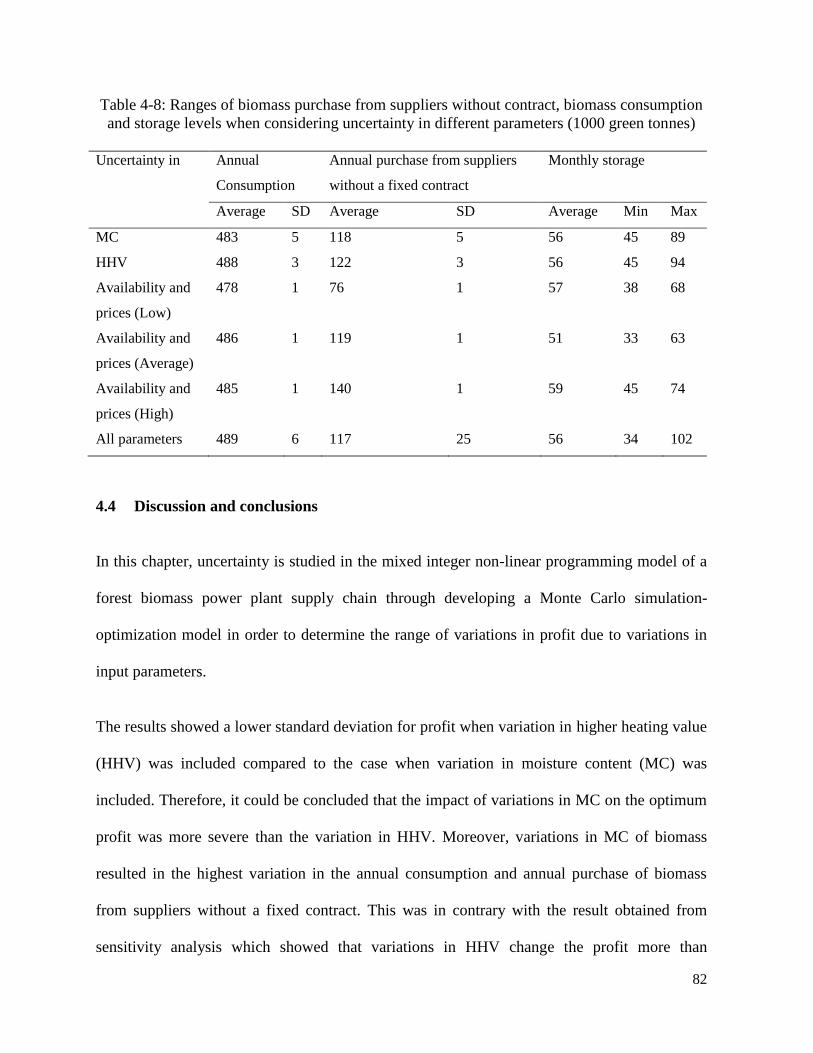
82
Table 4-8: Ranges of biomass purchase from suppliers without contract, biomass consumption
and storage levels when considering uncertainty in different parameters (1000 green tonnes)
Uncertainty in Annual
Consumption
Annual purchase from suppliers
without a fixed contract
Monthly storage
Average SD Average SD Average Min Max
MC 483 5 118 5 56 45 89
HHV 488 3 122 3 56 45 94
Availability and
prices (Low)
478 1 76 1 57 38 68
Availability and
prices (Average)
486 1 119 1 51 33 63
Availability and
prices (High)
485 1 140 1 59 45 74
All parameters 489 6 117 25 56 34 102
4.4 Discussion and conclusions
In this chapter, uncertainty is studied in the mixed integer non-linear programming model of a
forest biomass power plant supply chain through developing a Monte Carlo simulation-
optimization model in order to determine the range of variations in profit due to variations in
input parameters.
The results showed a lower standard deviation for profit when variation in higher heating value
(HHV) was included compared to the case when variation in moisture content (MC) was
included. Therefore, it could be concluded that the impact of variations in MC on the optimum
profit was more severe than the variation in HHV. Moreover, variations in MC of biomass
resulted in the highest variation in the annual consumption and annual purchase of biomass
from suppliers without a fixed contract. This was in contrary with the result obtained from
sensitivity analysis which showed that variations in HHV change the profit more than

83
variations in MC. The reason for that was that in sensitivity analysis the HHV and MC changed
within a same range (±20%), while variations in the historical data showed different ranges
with different probability distributions. These results showed that the Monte Carlo simulation
provided more realistic results that might differ from those ones obtained from sensitivity
analysis.
It was concluded that to have a profit of more than $15.0 M, the MC had to be less than 31%
for bark, 41% for sawdust, 24% for shavings and 37% for road logging debris (RLD).
Reducing MC to less than 28% for bark, 34% for sawdust, 10% for shavings and 25% for RLD
would increase the profit to $15.5 M, if all other parameters of the model remained the same.
This information would be helpful for the power plant supply manager when making supply
contracts and decisions on the drying of biomass because the amount of profit earned when
biomass was dried and had lower MC was shown.
The results indicated that when the electricity price was high (103.87 $/MWh), the profit
probability density function was more skewed to higher profit, while when the electricity price
was low (35.00 $/MWh), the profit distribution was more bell-shaped. This means that higher
electricity prices mitigate the impact of variations in cost and availability of biomass. The
results also showed that when all the uncertain parameters fluctuated at the same time, the
profit ranged between $13.4M and $17.9M with an average of $15.5M. Therefore, uncertainty
in the real system would resul i $4.5M varia io i he power pla ’s profi .
Uncertainty in biomass availability and cost and electricity prices, not the variability in
biomass quality (MC and HHV), resulted in the risks of having a profit lower than $14M and a
storage level below the minimum storage level, as well as the opportunity of having a profit

84
higher than $17M. Therefore, to mitigate the risks of having low profit and low storage levels,
it is needed to control uncertainties in the availability and prices.
This chapter addressed objective 3 of the thesis mentioned in 1.2. Historical data on important
uncertain parameters, which were identified previously through sensitivity analysis in 3.5.2
were analysed here. Uncertain parameters with different sources were grouped together and the
Monte Carlo simulation was implemented for each group as well as for all of them at the same
time. The profit distribution was determined when uncertain parameters varied based on their
distribution. Therefore, the output of this model represented the model behaviour when
uncertainty occurred and risks associated with uncertainties.
The Monte Carlo simulation method is a post-optimization approach, which means that the
decisions have to be made before this model is implemented and it only provides possible
changes in the decision variables and the profit in response to uncertainty. Taking uncertainty
into account when modeling the supply chain is a challenging task because the model becomes
complex and sometimes it may become computationally intractable especially if uncertainty is
included in different parameters simultaneously. Therefore, in the next chapter, uncertainty in
only one parameter, biomass availability, is included in the optimization model.

85
Chapter 5 Stochastic programming
5.1 Synopsis
So far, the impact of uncertainty on model solution has been evaluated through sensitivity
analysis and Monte Carlo simulation which are post-optimization approaches. In this chapter,
uncertainty is incorporated in the optimization model during the decision making process. This
is done by considering uncertainty in the monthly available biomass from different suppliers
during the planning horizon. The mixed integer non-linear programming model is first
reformulated into a mixed integer programming model. This enables a direct formulation of a
linear stochastic programming model. A two-stage stochastic programming model is developed
to maximize the expected profit of possible scenarios of available biomass. Two risk measures
are also included in the model to make the results more stable. The trade-off between
maximizing the profit and minimizing the risk is then evaluated.
5.2 The mixed integer programming model of the power plant supply chain
To facilitate incorporating uncertainty in the model, a new mixed integer linear programming
(MILP) model is proposed in this chapter. The main difference between the formulation of
MILP model in this chapter and the one developed in Chapter 3 is in the definition of the
storage and consumption variables. The notation of these variables is presented in Table 5-1.
Table 5-1: Decision variables of the linear programming model
Decision Variables
Amount of biomass stored in month from supplier (green tonnes)
Amount of biomass consumed in month from supplier (green tonnes)

86
The mixed integer linear model is as follows:
Objective function:
∑ (∑ )
∑ ∑ ∑ ∑ (5.1)
Here, Profit equals revenues minus costs as shown in Equation 5.1. Ash handling cost has
changed to ∑t AshHC × AshC × ∑s Cs,t.
The changes in the constraints are as follows:
The total storage level of biomass received and stored from all suppliers in month t has to be
less than or equal to the maximum storage level. Therefore, Equation 3.8 is changed to
Equation 5.2.
∑ [For all t] (5.2)
In the last month of the year, the total storage level of biomass from all suppliers has to be
equal to a target storage level. Therefore, Equation 3.9 is changed to Equation 5.3.
∑ (5.3)
The storage level of biomass received from supplier and stored in month t is equal to the
storage level of biomass received from supplier s and stored in previous month (t-1) plus
biomass purchase minus biomass consumption for the same supplier and month. For the first
time step, the initial storage level for each supplier has to be indicated. Therefore, Equation
3.10 is changed to Equation 5.4.

87
[For all s, t] (5.4)
In the MINLP model shown in Chapter 3, the decisions on purchase and consumption amounts
were not separated for each supplier because the total initial storage level was provided in the
obtained data. The initial energy value of the biomass in the storage was not provided and an
initial value for it in the MINLP was assumed. In the MILP model developed here, the initial
storage level for each supplier at the beginning of the planning horizon has to be known in the
mass balance equation for January (Equation 5.4). Therefore, it is assumed that the share of
biomass i he i i ial s orage level for each supplier is he same as each supplier’s share i he
total annual available biomass for the power plant in 2011. The initial average energy value in
the MILP is then calculated using those ratios.
Equation 3.12 is changed to Equation 5.5 to connect the energy demand in month t to the
biomass consumption variable. Et equals to the total biomass consumption for all suppliers in
month t multiplied by the total ratio of biomass type p for supplier s in month t, the energy
value of biomass type p from supplier s in month t, system efficiency, and the ratio of quality
reduction factor, if the storage level in month t is lower than SLL.
∑ ∑ [For all t] (5.5)
There is no need for variable AveEVt and Equation 3.13. It can be seen that constraint 5.5
contains the multiplication of a binary variable Zt and a continuous variable Cs,t. This non-
linear term can be converted to a linear constraint through replacing the term Zt×∑sCs,t by an
additional continuous variable, i.e. Lt≥0 and the following constraints 5.6, 5.7 and 5.8, where M
is a sufficiently large number.

88
[For all t] (5.6)
∑ [For all t] (5.7)
∑ [For all t] (5.8)
Having the above changes in the constraints and the objective function of the model presented
in Chapter 3 forms a mixed integer linear programming (MILP) model which was solved using
the AIMMS software package and the CPLEX solver.
5.3 The stochastic mixed integer programming model of the power plant supply chain
A two-stage stochastic programming approach is used here to deal with uncertainty in available
monthly biomass and incorporate it into the above multi-period planning model. In this
approach, it is assumed that at the beginning of the planning horizon, the available biomass
from each supplier for the first quarter of a year is known and it is uncertain for the rest of the
year. Therefore, the first stage includes the first three months (each period is a month) of a year
and the next nine months are considered as the second stage. The decision variables, including
the amount of biomass to be purchased from each supplier, the amount of biomass from each
supplier to be stored and the amount of biomass from each supplier to be consumed depend on
the available biomass, hence, these decision variables are considered as the first stage decision
variables in the first three months and the second stage decision variables in the next nine
months. The scenarios are made by varying the monthly available biomass from each supplier
by ±20% of the average scenario together with the expected volume, i.e. 3 different values. It is
assumed that the change in available biomass is stationary for three months since uncertainty in
available biomass is the result of fluctuation in lumber and other wood products market and the

89
market situation is assumed to be constant for that period. Consequently, the total number of
scenarios is 3 multiplied by the number of aggregated periods in the second stage, i.e. 33=27.
The general formulation for a two-stage stochastic programming is shown in the literature (e.g.
Birge & Louveaux (1997)) and is not repeated here. In this study, an implicit formulation of the
stochastic model for the forest biomass power plant supply chain is presented. This means that
there is one set of decision variables and the first stage decision variables are distinguished
from the second stage decision variables using non-anticipatory constraints.
There is a new set and a new parameter used in the developed two-stage stochastic model
defined as below:
Scenarios: List of scenarios (index i) {Scenario1, …, Scenario27}
: Maximum available biomass from supplier s in month t for scenario i.
Table 5-2 represents the definition of the stochastic model decision variables.
The objective function is to maximize the expected profit of all scenarios. To calculate the
expected value of profit, profit of scenario i (Profiti) is multiplied by Pri, the probability of
occurrence of scenario i (∑iPri =1), and the objective function is the sum of expected values as
shown in Equation 5.9.
∑
(5.9)
Here, Profiti equal revenues minus costs for scenario i as shown in Equation 5.10.

90
Table 5-2: Stochastic model decision variables
Amount of biomass purchased from supplier s in month t for scenario i (green tonnes), first
stage decision variable for t=1-3, and second stage decision variable for t=4-12.
Amount of biomass from supplier s stored in month t for scenario i (green tonnes), first stage
decision variable for t=1-3, and second stage decision variable for t=4-12.
Amount of biomass from supplier s consumed in month t for scenario i (green tonnes), first
stage decision variable for t=1-3, and second stage decision variable for t=4-12.
Amount of electricity generated in month t for scenario i (MWh), first stage decision variable
for t=1-3, and second stage decision variable for t=4-12.
Binary variable, 1 if surplus electricity is produced in a year, 0 otherwise for scenario i.
Binary variable, 1 if Ss,t,i is higher than the desired storage level (SDL) in month for scenario
i, first stage decision variable for t=1-3, second stage decision variable for t=4-12.
Binary variable, 1if Ss,t,i is higher than the upper storage limit (SUL) in month for scenario i,
first stage decision variable for t=1-3, and second stage decision variable for t=4-12.
Binary variable, 1 if Ss,t,i is less than lower storage limit (SLL) in month for scenario i, first
stage decision variable for t=1-3, and second stage decision variable for t=4-12.
∑ (∑ )
∑ ∑ ∑ ( ) ∑ (5.10)
Subject to:
Monthly available biomass for each supplier s with fixed contract in each month t and each
scenario i:
[For s∈{Supplier1, …, Supplier4}, all t and i] (5.11)

91
Monthly available biomass for each supplier s without fixed contract in each month t and each
scenario i:
[For s∈{Supplier5, …, Supplier8}, all t and i] (5.12)
Maximum storage level in each month t and each scenario i:
∑ [For all t and i] (5.13)
Last time period target storage level for each scenario i:
∑ [For t=Dec and all i] (5.14)
Mass balance equation for storage, consumption and purchase for each supplier s, each month t
and each scenario i:
[For all s, t and i] (5.15)
Energy demand in each month t and each scenario i:
∑
[For all t, i] (5.16)
Converting biomass to electricity in each month t and each scenario i:
∑ (∑ ) ( )
[For all t, i] (5.17)

92
And non-negativity of all variables for each supplier s, each month t and each scenario i:
, , , [for all s, t, i] (5.18)
In the stochastic programming model, it is assumed that at the start of each stage, the decision
makers have sufficient information on the amount of available biomass in that stage and can
adjust the production plan for that scenario. A decision xt is called implementable if it cannot
distinguish between different scenarios that are indistinguishable at a stage (Kazemi Zanjani et
al., 2010b). The constraints that are implying this are called non-anticipatively constraints as
follows.
, ,
[for t ∈{Jan,…,Mar}, all i and i' (i≠i') and s] (5.19)
5.4 Managing the risk
The output of a stochastic programming model is the total expected profit of all scenarios. This
model is risk-neutral because only the expected profit is considered in the formulation and
profit variations are ignored. The desired solution from a management perspective may include
decisions that generate higher than the expected profit or a desired target profit for a scenario.
Usually, decision makers are interested in knowing the potential risk and managing it while
optimizing the economic objective. To do this, different risk metrics can be defined and
included in the optimization model. In this paper, variability index and downside risk are
considered as two risk measures (You et al., 2009) and a weighted bi-objective model is
developed for the first risk measure. The objective functions are: to maximize the total
expected profit and minimize the risk measures.

93
5.4.1 Variability index
Uncertainty in input parameters of an optimization model results in uncertainty in the optimal
solution. Therefore, the solution, which in our case is profit, has mean and variance.
Considering the variance of the optimum solution in addition to its expected value is one of the
formula io s ha have bee called “robus op imi a io ” i he li era ure (Mulvey et al., 1995).
In this method, the variance of the total profit is minimized while the expected total profit is
maximized. However, using variance adds a quadratic term to the objective function which
makes the optimization model non-linear. Moreover, it treats the profits higher and lower than
the expected profit in the same way. Therefore, instead of variance in this study the negative
deviation between the scenario profit (Profiti) and the expected profit (Profit) is considered as
the risk measure as defined by Ahmed & Sahinidis (1998). The variability index is defined as a
non-negative continuous variable (∆i) for each scenario and the following constraint is added to
the model:
∑ [ , for all i] (5.20)
According to Equation 27, if the profit of scenario i (Profiti) is less than the expected profit
(Profit), ∆i is equal to their positive difference; otherwise it is 0. The objective function then is
to maximize the weighted sum of the total expected profit minus the expected variability index
as follows:
∑ ∑ ) (5.21)
94
Where ρ is the weight associated with the second objective function. The output of this bi-
objective model provides the trade-off between the expected profit and the profit variability
index.
5.4.2 Downside risk
When considering risk, the extremes of the optimum solutions are also important in addition to
their variability. It is desirable to have a lower probability of having low profit or a higher
probability of having high profit. To address this, another risk metric is used here called
downside risk, which is defined as the probability that the real profit is less than a certain
threshold or target Ω (You et al., 2009). The difference between the variability index defined
earlier and the downside risk is that in the latter the deviation is evaluated by comparing to a
target level while in the former it is compared to the expected profit. Here, the variable ψi is
defined as the positive deviation between the target Ω and the profit of scenario i (Profiti). If
the scenario profit (Profiti) is less than the target Ω, ψi is equal to their difference, otherwise it
is 0, as shown by the following constraints:
[ψi≥0, for all i] (5.22)
The following equation defines the downside risk metric associated with target Ω:
∑ (5.23)
In this case, Risk(Ω) is set to be equal to an appropriate predefined level and constraint 5.22 is
added to the model.

95
5.5 Results
5.5.1 Result of deterministic models
Based on the assumption for the initial storage explained in 5.3, the optimum profit for the
MILP model was $16.2M, 5% higher than that of the MINLP mode, which was $15.4M. It has
to be noted that there was no guarantee for the MINLP model to provide the exact optimal
solution since the model was not convex.
5.5.2 Results of the stochastic model
Table 5-3 shows the expected value of profit for three cases. Column 2 indicates the results if
perfect information on the scenario that is going to happen was available. In this case, the
deterministic model is solved for each scenario one by one. The average of profit for all
scenarios are calculated and shown in column 2 (scenario analysis model). However, in reality,
such perfect information is not available, and this is the motivation for developing a stochastic
model. Column 3 shows the expected profit for the stochastic model. The deterministic model
is usually solved using the average values for uncertain parameters. If the first stage decisions
based on average values are implemented, while other scenarios than the average scenario
occur in the second stage, the optimization model can be solved with implemented first stage
decisions to determine second stage decisions. Column 4 of Table 5-3 shows the expected
profit when the deterministic model is solved for each scenario using the first stage decisions of
the average scenario.

96
Table 5-3: Expected value of profit for scenario analysis, stochastic and average scenario
models ($M)
Deterministic
model –scenario
analysis
Stochastic
model
Deterministic model -
first stage decisions based
on average scenario
Expected value of profit 16.2 16.0 15.8
It can be seen that the expected value of profit for the scenario analysis is $16.2M which is
$0.2M higher than the expected value of profit for the stochastic model ($16.0M). This
difference is also called “Expected Value of Perfect Information” (EPVI) meaning that this is
the cost that the power plant is paying due to the existence of uncertainty in available biomass.
On the other hand, the expected value of profit of the stochastic model is $0.2M higher than the
expected value of profit for the case that the deterministic model result for the average scenario
is implemented but other scenarios occur. This difference is named “Value of Stochastic
Solution” (VSS) and represents the profit that is associated with inclusion of uncertainty in
available biomass and justifies using more sophisticated methods such as stochastic
programming in production planning of the power plant (Birge & Louveaux, 1997).
Figure 5-1 shows the histogram of profit for using average scenario results and stochastic
model.
It can be seen that the standard deviation of the average scenario is lower than that of the
stochastic model. It also indicates that the frequency of having very high profit ($17-18M) and
very low profit ($12-13M) is higher in the case of the stochastic model while there is a higher
probability of having profit in the range of $16-17M in the deterministic model using average
scenario results for the first stage decisions.
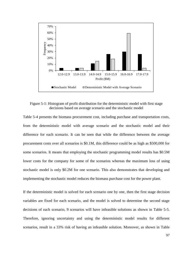
97
Figure 5-1: Histogram of profit distribution for the deterministic model with first stage
decisions based on average scenario and the stochastic model
Table 5-4 presents the biomass procurement cost, including purchase and transportation costs,
from the deterministic model with average scenario and the stochastic model and their
difference for each scenario. It can be seen that while the difference between the average
procurement costs over all scenarios is $0.1M, this difference could be as high as $500,000 for
some scenarios. It means that employing the stochastic programming model results has $0.5M
lower costs for the company for some of the scenarios whereas the maximum loss of using
stochastic model is only $0.2M for one scenario. This also demonstrates that developing and
implementing the stochastic model reduces the biomass purchase cost for the power plant.
If the deterministic model is solved for each scenario one by one, then the first stage decision
variables are fixed for each scenario, and the model is solved to determine the second stage
decisions of each scenario, 9 scenarios will have infeasible solutions as shown in Table 5-5.
Therefore, ignoring uncertainty and using the deterministic model results for different
scenarios, result in a 33% risk of having an infeasible solution. Moreover, as shown in Table
0%
10%
20%
30%
40%
50%
60%
70%
12.0-12.9 13.0-13.9 14.0-14.9 15.0-15.9 16.0-16.9 17.0-17.9
Fre
quen
cy
Profit ($M)
Stochastic Model Deterministic Model with Average Scenario

98
5-5 the average profit for those scenarios with feasible results are always less than that of the
stochastic solution, which is $16.0M.
Table 5-6 indicates the standard deviation of the amount of biomass consumption, which is one
of the decision variables of the model, of 27 scenarios for each month from all suppliers, for
both the deterministic scenario analysis and the stochastic model. It can be seen that for the
stochastic model the standard deviation is zero for the first stage decisions, as expected from
definition of non-anticipatory constraints. The decision variables are therefore independent of
the scenario occurring in the future which makes them implementable. The same table can be
presented for other decision variables, such as the amount of biomass purchased in each month.
Other remarks from the results are as follows. In the scenario analysis model, the optimization
results indicate that the surplus load should not be produced for three scenarios, while in the
stochastic model the surplus load is always produced. Moreover, the storage level never go
beyond the upper and lower limits ( , and ) neither in stochastic nor in
deterministic models. Therefore, there is no risk of having very low or very high storage levels
related to the uncertainty in available biomass.
It should be noted that the model and the above comparisons are related to a process where
decisions on the first stage are used and implemented. It is possible that after implementing the
first three months, the system is re-planned with a new stochastic model over the rest of the
year, i.e. 3+6 months as the new first and second stages.

99
Table 5-4: Biomass procurement cost for each scenario of stochastic and deterministic models
($M)
Scenario Stochastic Model
(SM)
Deterministic Model -
Average Scenario (DM)
Difference
(SM-DM)
S1 6.7 7.0 -0.5
S2 6.9 7.4 -0.5
S3 7.2 7.6 -0.4
S4 7.0 7.5 -0.5
S5 7.2 7.7 -0.5
S6 8.0 8.0 0.0
S7 7.4 7.8 -0.4
S8 8.2 8.1 0.1
S9 9.1 9.0 0.1
S10 7.0 7.5 -0.5
S11 7.2 7.7 -0.5
S12 7.9 7.9 0.0
S13 7.4 7.8 -0.4
S14 8.1 8.1 0.0
S15 9.0 8.9 0.1
S16 8.4 8.3 0.1
S17 9.2 9.1 0.1
S18 10.1 10.0 0.1
S19 7.4 7.8 -0.4
S20 8.1 8.1 0.0
S21 9.0 8.9 0.1
S22 8.4 8.3 0.1
S23 9.2 9.1 0.1
S24 10.1 10.0 0.1
S25 9.4 9.3 0.1
S26 10.3 10.2 0.1
S27 11.3 11.1 0.2
Average 8.3 8.4 -0.1

100
Table 5-5: Average profit if the first stage decision variables of each scenario is implemented
and other scenarios happen ($M)
Scenario which its first stage
decisions are implemented
Expected value if other 26 scenarios
happen
S1 Infeasible
S2 Infeasible
S3 Infeasible
S4 Infeasible
S5 Infeasible
S6 15.8
S7 15.9
S8 15.8
S9 15.7
S10 Infeasible
S11 Infeasible
S12 15.9
S13 15.9
S14 15.8
S15 15.5
S16 15.8
S17 15.4
S18 Infeasible
S19 15.9
S20 15.8
S21 15.5
S22 15.8
S23 15.4
S24 15.3
S25 15.3
S26 15.3
S27 Infeasible
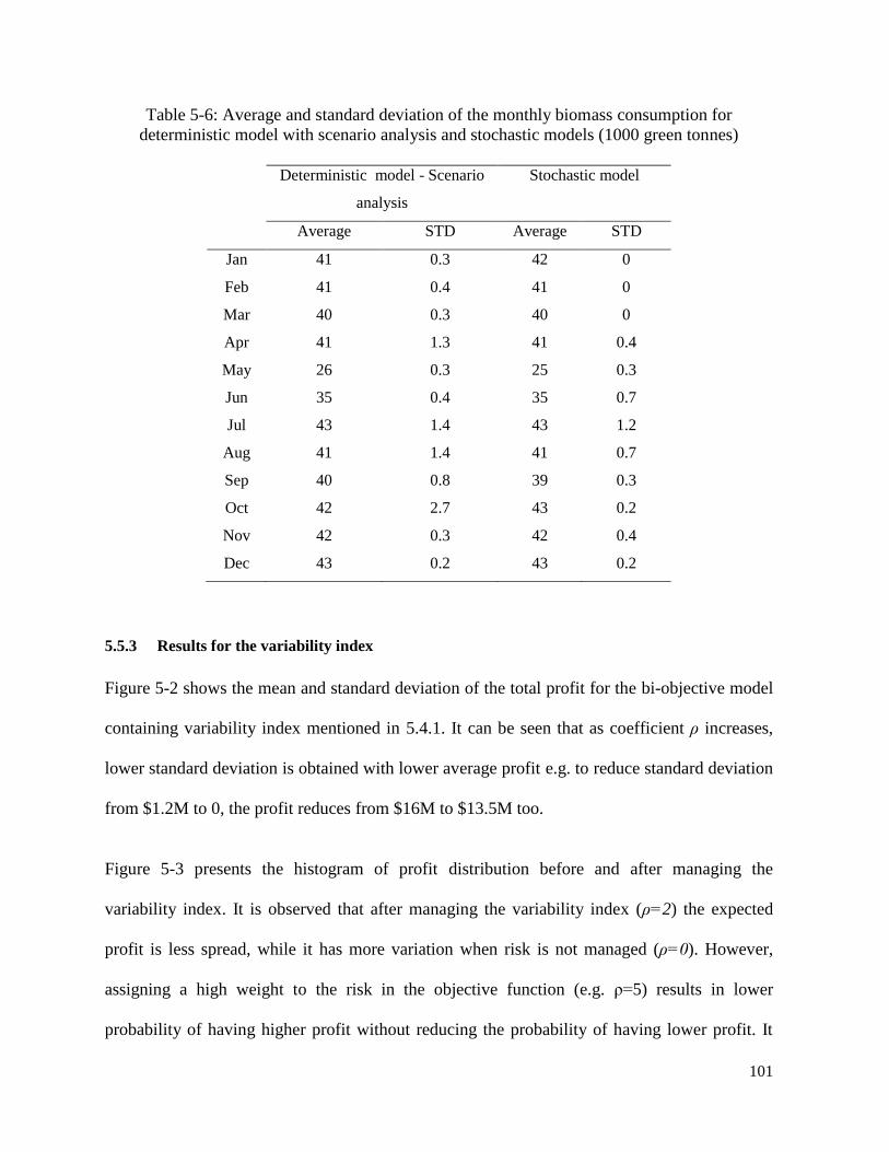
101
Table 5-6: Average and standard deviation of the monthly biomass consumption for
deterministic model with scenario analysis and stochastic models (1000 green tonnes)
Deterministic model - Scenario
analysis
Stochastic model
Average STD Average STD
Jan 41 0.3 42 0
Feb 41 0.4 41 0
Mar 40 0.3 40 0
Apr 41 1.3 41 0.4
May 26 0.3 25 0.3
Jun 35 0.4 35 0.7
Jul 43 1.4 43 1.2
Aug 41 1.4 41 0.7
Sep 40 0.8 39 0.3
Oct 42 2.7 43 0.2
Nov 42 0.3 42 0.4
Dec 43 0.2 43 0.2
5.5.3 Results for the variability index
Figure 5-2 shows the mean and standard deviation of the total profit for the bi-objective model
containing variability index mentioned in 5.4.1. It can be seen that as coefficient ρ increases,
lower standard deviation is obtained with lower average profit e.g. to reduce standard deviation
from $1.2M to 0, the profit reduces from $16M to $13.5M too.
Figure 5-3 presents the histogram of profit distribution before and after managing the
variability index. It is observed that after managing the variability index (ρ=2) the expected
profit is less spread, while it has more variation when risk is not managed (ρ=0). However,
assigning a high weight to the risk in the objective function (e.g. ρ=5) results in lower
probability of having higher profit without reducing the probability of having lower profit. It

102
means that although the standard deviation of profits of different scenarios has been reduced,
they are distributed around a lower expected value. Therefore, it is not reasonable to assign
high weight to the risk in the objective function.
Figure 5-2: Profit mean and standard deviation for different weights (ρ)
Figure 5-3: Histogram of profit distribution for different weights (ρ) associated with variability
index
0
0.2
0.4
0.6
0.8
1
1.2
1.4
12
12.5
13
13.5
14
14.5
15
15.5
16
16.5
0 1 2 5 7 10 20 27
Sta
nd
ard
Dev
iati
on (
$M
)
Pro
fit
($M
)
ρ
Profit STDV
0%
10%
20%
30%
40%
50%
60%
70%
80%
90%
12.0-12.9 13.0-13.9 14.0-14.9 15.0-15.9 16.0-16.9 17.0-17.9
Fre
quen
cy
Profit ($ M)
ρ=0 ρ=2 ρ=5
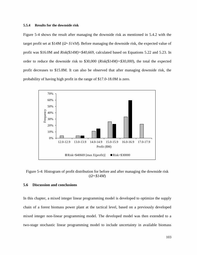
103
5.5.4 Results for the downside risk
Figure 5-4 shows the result after managing the downside risk as mentioned in 5.4.2 with the
target profit set at $14M (Ω=$14M). Before managing the downside risk, the expected value of
profit was $16.0M and Risk($14M)=$40,669, calculated based on Equations 5.22 and 5.23. In
order to reduce the downside risk to $30,000 (Risk($14M)=$30,000), the total the expected
profit decreases to $15.8M. It can also be observed that after managing downside risk, the
probability of having high profit in the range of $17.0-18.0M is zero.
Figure 5-4: Histogram of profit distribution for before and after managing the downside risk
(Ω=$14M)
5.6 Discussion and conclusions
In this chapter, a mixed integer linear programming model is developed to optimize the supply
chain of a forest biomass power plant at the tactical level, based on a previously developed
mixed integer non-linear programming model. The developed model was then extended to a
two-stage stochastic linear programming model to include uncertainty in available biomass
0%
10%
20%
30%
40%
50%
60%
70%
12.0-12.9 13.0-13.9 14.0-14.9 15.0-15.9 16.0-16.9 17.0-17.9
Fre
quen
cy
Profit ($M)
Risk=$40669 [max E(profit)] Risk=$30000

104
from different suppliers. The results of the case study showed that having the perfect
information about monthly available biomass from suppliers, he power pla ’s a ual profi
would be $16.2M. However, in reality, the amount of available biomass from supplier varies
due to a number of factors such as market fluctuations resulting in an average profit of $15.8M,
$0.4M lower than $16.2M. Part of this loss could be compensated using a stochastic
programming model. The profit of the stochastic model was $0.2M higher than the solution
when the average scenario was implemented while other scenarios occurred and $0.2M lower
than the solution of the deterministic model with the perfect information. The procurement cost
of the stochastic model was $0.5M lower than that of the average scenario. The reason that the
stochastic model had lower profit than the deterministic model was that in the stochastic
optimization, the expected value over all scenarios of monthly available biomass, including the
scenarios with 20% reduction in supply, were optimized. In addition, ignoring uncertainty and
implementing deterministic model results for each scenario resulted in a 33% chance of having
an infeasible solution. Moreover, the stochastic model decision variables were implementable
since they did not depend on future uncertainties. This was obtained, however, with a more
sophisticated model, higher amount of computational effort and the need for data and
assumptions about uncertain parameters.
Two risk measures were also considered in this study and two models were developed and
solved in order to explicitly consider the risks included in the supply chain planning process.
The considered risk measures were the variability index and downside risk. The results of risk
management models indicated that the total expected profit of the power plant would reduce
after risk management. Lower profit variance was obtained by managing the variability index,
but it resulted in lower probability of having higher profit. When the downside risk is

105
controlled, the probability of having very low and very high profit decreased. It is important to
manage risk measures properly in order to prevent low expected values for profit. Basically,
this is up to the power plant managers to decide on the risk measures as well as the risk
threshold that are acceptable to them, and then implement the optimum solution of using those
risk measures and thresholds in the models.
This chapter addressed the thesis fourth objective partially by including uncertainty in biomass
availability in a two-stage stochastic optimization model. It is important to incorporate the
uncertainty in biomass quality into the modeling to have a comprehensive robust model in
response to uncertainty. This is done in the next chapter.

106
Chapter 6 Hybrid stochastic programming-robust optimization model
6.1 Synopsis
In the previous chapter, uncertainty in one parameter, biomass availability, was included in the
optimization model. In this chapter, uncertainty in several parameters of the power plant supply
chain is incorporated simultaneously. Uncertain parameters incorporated here are biomass
quality, namely moisture content and higher heating value, in addition to monthly available
biomass from suppliers. Uncertainties in electricity prices and biomass cost are not included
because the power plant has long term contracts with the client and most of the suppliers. This
means the prices and costs do not change during the planning horizon. i.e. a year. There is a
small variation in biomass cost over a year for suppliers without a fixed contract, therefore,
uncertainty in biomass cost for those suppliers can be ignored as well.
Moisture content and higher heating value change within a range and are considered in a
developed robust optimization model. Uncertainty in monthly available biomass is included
through a two-stage stochastic programming model as explained in Chapter 5. A hybrid
stochastic programming-robust optimization model is used to incorporate uncertainty in all of
the mentioned parameters simultaneously, and to have an appropriate balance between
computational complexity associated with the stochastic programming formulation and
conservatism of the optimal solution (lower profit) associated with the robust optimization
approach.
6.2 Robust optimization formulation
Two indicators of biomass quality are considered here: moisture content (MC) in % and higher
heating value (HHV) in BTU/lb. These parameters are not correlated since HHV is calculated

107
based on dry biomass. Energy value depends on MC and HHV as was shown in Equation 3.14.
Based on the historical data provided by the power plant, the range of variation is considered to
be 25-35% for MC with an average of 30%, and 8000-9000 BTU/lb (5.17-5.81 MWh/tonnes)
for HHV with an average of 8500 BTU/lb (5.49 MWh/tonnes). To be able to include
uncertainty in MC and HHV in a stochastic programming model, different scenarios can be
obtained for them by discretizing their ranges. However, if these scenarios are combined with
the 27 scenarios of monthly available biomass, the total number of scenarios is going to be
huge even with a small number of discretized scenarios. For instance, considering only 3
scenarios for each of MC and HHV, within the scenario structure described above for monthly
available biomass, the number of scenarios will be 93×27=19683. This is even without
considering the combination of different MC and HHV for different suppliers. Therefore,
robust optimization is used to include uncertainty in biomass quality into the decision making
process.
The formulation for the robust optimization is derived from Ben-Tal et al. (2009) which is
available in the AIMMS software package. It helps to come up with a tractable model
providing a solution that is feasible for all MC and HHV ranges with a price of having lower
profit since the worst case is optimized. Here, a brief explanation of the idea of robust
optimization is provided.
Consider a general linear programming (LP) model as shown in Equation 6.1:
(6.1)

108
Where x represent model decision variables, c is the objective function coefficients vector, b is
the right hand side values vector and A is the constraints coefficient matrix. If the parameters of
the model, c, A and b, are uncertain and range within a convex set of U, then the robust
counterpart of this uncertain LP model can be defined as shown in Equation 6.2:
∈ ∈ ∈ (6.2)
It should be noted that in robust optimization, the objective is to optimize the worst case.
Equation 6.2 can be reformulated as follows:
∈ ∈ ∈ (6.3)
The robust counterpart model shown in Equation 6.3 has a single objective function and
continuous constraints. Any solution for Equation 6.3 satisfies the constraints of
Equation 6.2 for c, A and b∈U. These solutions are robust feasible and among such robust
feasible solutions, the robust optimal value, namely , is the one providing the best possible
objective function for Equation 6.3. Ben-Tal & Nemirovski (2002) proved that problem shown
in Equation 6.3 is computationally tractable (or in the other words polynomially solvable) for a
wide choice of the uncertainty sets U. Particularly, problem in Equation 6.3 is an LP model if
U is a box or polyhedral set (Li & Floudas). Without loss of generality, only uncertainty in
parameters of matrix A, named as is considered. If belongs to a box set, the uncertainty in
is defined as:
(6.4)

109
where is the nominal value of parameters and is the positive constant perturbation and is
independent random variables which are subject to uncertainty. Then, constraint –
can be written as:
∑ ∑ (6.5)
The solution has to be feasible for any in a given uncertainty set U or alternatively:
∑ ∈ ∑ (6.6)
In particular for the box uncertainty set the random vector is defined as:
(6.7)
Where is an adjustable parameter controlling the size of uncertainty set. Then the
corresponding robust counterpart in Equation 6.3 is equivalent to the following constraints:
∑ ∑ – (6.8)
(6.9)
Where u is a decision variable (u≥0). Equation 6.9 is still linear (Li & Floudas). In the present
model, uncertain parameters belong to certain ranges and therefore can be considered as box.
This formulation is being used to include uncertainty in biomass quality in the optimization
model presented in this thesis. The MILP model presented in Chapter 5 is first extended to a
robust optimization model. The formulation for robust optimization model, in case of
uncertainty only in MCs,p,t is included is as follows:
(6.10)

110
∑ (∑ ) ∑
∑ ∑ ∑ (6.11)
Subject to:
[For s∈{Supplier1, …, Supplier4} and all t] (6.12)
[For ∈{Supplier5, …, upplier8} and all t] (6.13)
∑ [For all t] (6.14)
∑ (6.15)
[For all s and t] (6.16)
∑
[For all t] (6.17)
∑ ∑ –
[For ∈[25,30] and all t] (6.18)
All continuous variables have to be non-negative as shown in Equation 6.19.
, , , [for all s, t] (6.19)
Notice that constraint (6.18) is converted to inequality in order to make sure it can be met for
all realization of .

111
The robust counterpart of Equation 6.18 is as follows (according to Equations 6.8 and 6.9):
∑ (∑
( )) –
∑ (∑
) –
[for all t] (6.20)
, (6.21)
Where s,p,t is the positive constant perturbation in MCs,p,t and ψ is the adjustable parameter
controlling the size of uncertainty set. The same formulation can be written for uncertainty in
HHVs,p,t. When uncertainty in both parameters is included, the term HHVs,p,t × (1 – MCs,p,t) is
replaced by EVs,p,t and the formulation is written for this parameter with the range derived from
ranges in both HHVs,p,t and MCs,p,t.
6.3 Hybrid stochastic programming-robust optimization model
Here, the formulation for hybrid stochastic programming-robust optimization model, in case of
uncertainty in MCs,p,t only, is presented:
(6.22)
∑ (∑ ) ∑
∑ ∑ ( ) ∑ (6.23)

112
Subject to:
[For s∈{Supplier1, …,Supplier4}, all t and i] (6.24)
[For s∈{Supplier5, …,Supplier8}, all t and i] (6.25)
∑ [For all t and i] (6.26)
∑ [For t=Dec and all i] (6.27)
[For all s, t and i] (6.28)
∑
[For all t, i] (6.29)
∑ ∑ –
[For ∈[25,30] and all t and i] (6.30)
All continuous variables have to be non-negative as shown in Equation 6.19.
, , , [for all s, t, i] (6.31)
Again, constraint (6.30) is converted to inequality in order to make sure it can be met for all
realization of .
The robust counterpart of Equation 6.30 is as follows:

113
∑ (∑ ) ( – )
∑ (∑ ) ( – )
(6.32)
(6.33)
The same formulation can be written for uncertainty in HHVs,p,t. When uncertainty in both
parameters is included, the term HHVs,p,t×(1-MCs,p,t) is replaced by EVs,p,t and the formulation
is written for this parameter with the range derived from ranges in both and .
6.4 Results
First, the results of the robust optimization model are presented where variations in biomass
quality are considered. A solution that is feasible for all possible instances of uncertain
parameters will likely be a conservative solution. The model is solved with different ranges for
MCs,p,t and HHVs,p,t values to assess how the solution changes when the uncertainty set is
widened, the results can be seen in Table 6-1. The profit of the robust optimization model using
the average MCs,p,t (30%) and average HHVs,p,t (8500 BTU/lb) is $15.64M. Using the average
HHVs,p,t in the model, as the uncertainty set of MC widens from 2% to 10%, the optimum profit
drops from $15.07M to $13.13M, which is also shown in Figure 6-1. Alternatively, using the
average MCs,p,t of 30% in the model, as the uncertainty set of HHVs,p,t is expanded from 200
BTU/lb (0.13 MWh/tonnes) to 2000 BTU/lb (1.29 MWh/tonnes), the optimum profit reduces
from $15.15M to $13.58M, as shown in Figure 6-2. When both parameters are considered
uncertain at the same time, the result becomes more conservative with a more severe reduction
in profit to $11.97M for HHVs,p,t∈[8100,8900], MCs,p,t∈[26,34]. In the extreme ranges, the
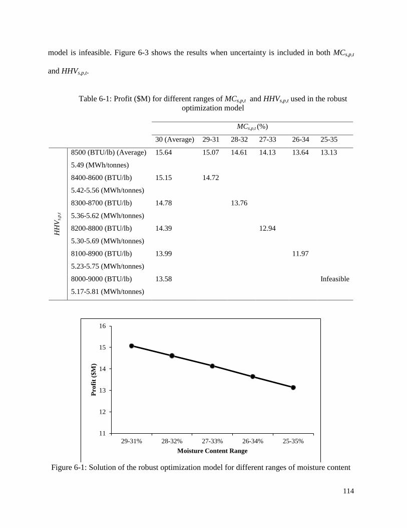
114
model is infeasible. Figure 6-3 shows the results when uncertainty is included in both MCs,p,t
and HHVs,p,t.
Table 6-1: Profit ($M) for different ranges of MCs,p,t and HHVs,p,t used in the robust
optimization model
MCs,p,t (%)
30 (Average) 29-31 28-32 27-33 26-34 25-35
HH
Vs,
p,t
8500 (BTU/lb) (Average)
5.49 (MWh/tonnes)
15.64 15.07 14.61 14.13 13.64 13.13
8400-8600 (BTU/lb)
5.42-5.56 (MWh/tonnes)
15.15 14.72
8300-8700 (BTU/lb)
5.36-5.62 (MWh/tonnes)
14.78 13.76
8200-8800 (BTU/lb)
5.30-5.69 (MWh/tonnes)
14.39 12.94
8100-8900 (BTU/lb)
5.23-5.75 (MWh/tonnes)
13.99 11.97
8000-9000 (BTU/lb)
5.17-5.81 (MWh/tonnes)
13.58 Infeasible
Figure 6-1: Solution of the robust optimization model for different ranges of moisture content
11
12
13
14
15
16
29-31% 28-32% 27-33% 26-34% 25-35%
Pro
fit
($M
)
Moisture Content Range

115
Figure 6-2: Solution of the robust optimization model for different ranges of higher heating
value
Figure 6-3: Solution of the robust optimization model for different ranges of energy value
Despite having a more conservative solution with a lower profit, the decisions provided by
robust optimization are feasible for ranges of MC and HHV shown in Figure 6-3. The model
was run for the case where the decision variables of biomass purchase, storage and
consumption in the first three months are made and implemented based on the results of the
model using average MC and HHV (MCs,p,t=30% and HHVs,p,t=8500 BTU/lb). Then, it was
11
12
13
14
15
16
8400-8600 8300-8700 8200-8800 8100-8900 8000-9000
Pro
fit
($M
)
Higher Heating Value Range (BTU/lb)
11
12
13
14
15
16
29-31%
8400-8600
28-32%
8300-8700
27-33%
8200-8800
26-34%
8100-8900
Pro
fit
($M
)
Moisture Content Range
Higher Heating Value Range (BTU/lb)

116
assumed that for the rest of the months, MC and HHV take other values (any of the ranges
showed in Table 6-1, for instance HHVs,p,t∈[8100,8900] and MCs,p,t∈[26,34]). It was observed
that the model becomes infeasible when MCs,p,t and HHVs,p,t vary from their average values,
which in reality is very probable.
Figure 6-4 and Figure 6-5 show the optimum biomass storage and consumption level in
different months based on the results of the robust optimization model with
HHVs,p,t∈[8100,8900], MCs,p,t∈[26,34] and the deterministic model. It can be seen that robust
optimization provides more storage levels compared to the deterministic model for most of the
months and more consumption levels in all months. The consumption level is higher due to a
lower than average energy value of biomass used in the robust optimization model.
Figure 6-4: The optimum storage level in different months from the robust optimization model
with HHVs,p,t∈[8100,8900] and MCs,p,t∈[26,34] and the deterministic model
0
10
20
30
40
50
60
70
80
90
Jan Feb Mar Apr May Jun Jul Aug Sep Oct Nov Dec
Sto
rag
e L
evel
(1
00
0 G
reen
To
nn
es)
Robust Optimization
Deterministic

117
Figure 6-5: The optimum biomass consumption level in different months from the robust
optimization model with HHVs,p,t∈[8100,8900] and MCs,p,t∈[26,34] and the deterministic
model
The result of the hybrid stochastic programming-robust optimization model is provided in
Table 6-2. The first two columns show MC and HHV ranges. The next columns show the
robust optimization solutions, the hybrid stochastic programming-robust optimization solutions
and their differences, respectively. It can be seen that the hybrid stochastic programming-
robust optimization model provides a more conservative solution compared to the robust
optimization model. However, the reduction in profit is small (0.2-0.7%). The reduction in
profit increases as the range of uncertainty decreased. For the average values of HHV and MC,
the profit for the deterministic model is $15.64M and it is $15.45M for the stochastic
programming model.
Despite having a lower profit from the hybrid stochastic programming-robust optimization
model, it provides feasible solutions for all scenarios of monthly available biomass and all
ranges of variation in MC and HHV. Figure 6-6 shows the optimum storage level over 27
scenarios for the robust optimization model and the hybrid stochastic programming-robust
optimization model when HHVs,p,t∈[8100,8900] and MCs,p,t∈[26,34]. To make the graphs
0
10
20
30
40
50
Jan Feb Mar Apr May Jun Jul Aug Sep Oct Nov Dec
Bio
ma
ss C
on
sum
pti
on
(1
00
0 G
reen
To
nn
es)
Robust Optimization
Deterministic

118
readable, only the storage levels from January to May are depicted. It can be seen that the first
stage decision variables are unique and independent when stochastic programming is used.
Table 6-2: Profit for different ranges of MCs,p,t and HHVs,p,t used in the robust optimization and
hybrid models
MCs,p,t
range (%)
HHVs,p,t range
(BTU/lb)
Robust optimization
solution ($M)
Hybrid model
solution ($M)
Difference
($M)
26-34 8100-8900 11.97 11.93 0.03
27-33 8200-8800 12.94 12.87 0.07
28-32 8300-8700 13.76 13.66 0.10
29-31 8400-8600 14.72 14.61 0.11
Figure 6-6: Optimum storage level of 27 scenarios for the first five months for a) robust
optimization model, and b) hybrid stochastic programming-robust optimization model when
HHVs,p,t∈[8100,8900] and MCs,p,t∈[26,34]
6.5 Discussion and conclusions
In this chapter, first uncertainty in biomass quality is included in the optimization model of a
forest bioenergy supply chain through developing a robust optimization model. This model
provides a solution that is feasible for any value of uncertain parameters within a defined
range. Different profit can be generated depending on the variation range for MC and HHV.
For the average MC (30%) and average HHV (8500 BTU/lb), the profit was $15.64M. For
40
50
60
70
80
90
100
Jan Feb Mar Apr May
Sto
rag
e (1
00
0 G
reen
To
nn
es)
40
50
60
70
80
90
100
110
120
Jan Feb Mar Apr May
Sto
rag
e (1
00
0 G
reen
To
nn
es)

119
average HHV and MC range of 29-31%, the profit decreased to $15.07M, while it dropped to
$13.13M for MC range of 25-35%. When HHV changed within 200 BTU/lb range (8400-8600
BTU/lb) with the average MC, the optimum profit reduced to $15.15M. It also decreased to
$13.58M, as the HHV range was widened to (8000-9000 BTU/lb). When MC and HHV
changed simultaneously the solution became more conservative. For instance, the profit for the
widest range with a feasible solution, which was (26-34%) for MC and (8100-8900 BTU/lb)
for HHV, was $11.97M. From these results, it was concluded that as the range of uncertain
parameters widened, the profit obtained from the robust optimization model decreased. The
reason was that in the robust optimization model, the worst case scenario was optimized.
Expanding the range of the uncertain parameters made the worst case scenario worse.
A hybrid stochastic programming-robust optimization model was then proposed to incorporate
uncertainties in different parameters simultaneously. Stochastic programming was used to
include uncertainty in monthly available biomass using 27 scenarios over a one-year time
horizon. Robust optimization was used to model the uncertainty in biomass quality within a
polyhedral set. Comparing the results of robust optimization and stochastic programming
models, it can be concluded that the conservatism in the robust optimization model was more
severe because it optimized the worst cases while the stochastic programming model optimized
the expected value of all scenarios. The degree of conservatism can be controlled by selecting
the appropriate range of uncertain parameters. The conservative solution was compensated by
having more stable solution which was free of infeasibility risk. No matter what happens in
terms of uncertain parameter values, one can be sure that the model remains feasible and the
decisions can be adjusted if any perturbation occurs within the defined sets or scenarios. To
balance the conservatism of optimizing the worst case, stochastic programming was used to

120
include uncertainty in available biomass. When the hybrid model was implemented, the profit
reduced even more. For instance, for the case with (26-34%) range for MC and (8100-8900
BTU/lb) range for HHV, the profit was $11.93M, $0.03M lower than that of the robust
optimization model with the same ranges, $11.97M. However, this model has the advantage of
providing a solution which is implementable, e.g. unique decision variables for the first stage.
The stochastic programming results have the advantage of being unique for the first stage, or in
other words, being implementable.
This chapter completed on the fourth objective of the thesis. Making decisions in supply chain
planning at the tactical level considering uncertainty in biomass quality was unavailable before.
The hybrid model is a unique approach to include uncertainty in several parameters
simultaneously and balance the advantages and disadvantages of both stochastic programming
and robust optimization approaches.

121
Chapter 7 Conclusions, strength points, limitations and future research
7.1 Conclusions
The optimization models developed and presented in Chapters 3-6 achieved all the objectives
of this study. The deterministic model presented in Chapter 3 achieved objectives 1 and 2 and
part of objective 3, the Monte Carlo simulation model presented in Chapter 4 fully achieved
objective 3 and the stochastic programming, robust optimization and the hybrid model
developed and presented in Chapters 5 and 6 achieved the 4th
objective.
From the deterministic model presented in Chapter 3 it was concluded that optimization models
were useful tools that could help managers of forest biomass power plants to make better
decisions on how much biomass to purchase, store and consume in each month to meet the
electricity demand and maximize their profit. Different parts of the supply chain from biomass
supply to storage and electricity production, were integrated in the deterministic model,
therefore, the optimum solution prescribed by the model was based on the impact of parameters
in all parts of the supply chain and the interactions between different supply chain parts. This
would be helpful for decision makers because it would not be possible for them (without using
a decision support tool) to consider all these factors and interactions simultaneously when
making decisions. In fact, the decisions in the power plant are made by different people (fibre
manager, production manager, and some by finance manager). The managers make their own
decisions and then have quarterly meetings to discuss important issues without being able to
know how each decision would affect other decisions or the profit as a whole. The model
developed here is useful since it integrates all the supply chain parts.
The impact of uncertainty in input parameters on the profit was shown from sensitivity analysis
results. These results showed that variations in electricity price, higher heating value,
maximum available biomass from suppliers with fixed contracts, moisture content and biomass
122
cost had high impacts on the optimum solution. The results of the Monte Carlo simulation
model showed that variation in moisture content had a higher impact on profit than variation in
higher heating value.
Including uncertainty in the decision making process may seem to provide lower profit for the
power plant. However, it provided a robust solution against perturbations in input parameters.
The solution was feasible for all considered instances of uncertain parameters and was
implementable. It was also concluded that there was a trade-off between expected value of
profit and probability of having low profit. Moreover, it was shown that developing a hybrid
model that was a combination of stochastic programming and robust optimization models
provided a flexible framework for considering uncertainty in different parameters at the same
time. The hybrid model took advantage of both stochastic programming and robust
optimization models; it is computationally tractable and not too conservative. If the hybrid
model is implemented, the power plant managers would make sure even with the changes in
the parameters (biomass availability and quality), that are probable in reality, the power plant
still would be able to generate electricity and meet the demand, have biomass for production
and do not have shortage or an excess storage.
7.2 Strengths points
The main strength and contribution of this thesis is that the issue of uncertainty which is a
critical factor in the forest biomass supply chain is incorporated in the modeling and analysis
comprehensively. This can be used as a guideline for dealing with uncertainty in forest
biomass/ bioenergy supply chains, or even other supply chains that have a similar structure.
The case study presented here, is a real forest biomass power plant. Having access to real data
and being able to communicate with people working directly in this industry is a strength point

123
of this research. The model structure and solutions were validated by the power plant
managers. Moreover, data analysis, particularly probability distribution of biomass quality for
different biomass types in different months, provided useful information that could be used in
other relevant studies.
The only study similar to this work was conducted by Alam et al. (2012b). They developed an
optimization model with monthly time steps for supply chain management of a forest biomass
power plant. The main difference between this deterministic optimization model and the one
developed by Alam et al. (2012b) is that in the former, biomass quality for each biomass types,
from each suppliers and in each months is considered to be different. This allows variations in
biomass availability and quality during the year to be included in the optimization model. Alam
et al. (2012b) used an average value for energy value and moisture content in all months.
Moreover, they focused more on the harvesting side of the supply chain while the model
developed here included the whole supply chain from procurement to storage, production and
ash management. It also included the effects of mixing biomass and storage on biomass quality
and production efficiency which were not done before, even in studies of other forest bioenergy
plants such as district heating systems or biofuel plants.
Most of the time, uncertainty is ignored due to the lack of data, complexity of models with
uncertainty, and difficulty to solve them. All the studies in forest biomass power plants supply
chains ignored uncertainty. Alam et al. (2012b) only evaluated the impact of uncertainty in the
parameters of an optimization model of a forest biomass power plant only through sensitivity
analysis. They did not include uncertainty in the modeling and decision making process. In this
thesis, historical data were used for identifying and quantifying uncertainty in different
parameters. Ignoring uncertainty in parameters gave infeasible solutions (33% of the cases),

124
which means the constraints of the model (supply, demand, storage, etc.) were not met. The
approaches for dealing with uncertainties were selected based on the model structure,
characteristics of uncertain parameter, the quality of the solution they provided, and the
computational effort needed to solve them. In the literature, there were studies that developed
stochastic programming models to include uncertainty in similar industries, such as biofuel
supply chains. However, all of them were at the strategic level with one time step. In the
present study, the stochastic programming model was developed and solved for a multiple time
step problem, which is more complex. Developing a hybrid stochastic programming–robust
optimization model to incorporate uncertainty in different parameters of the supply chain was
also a novel idea in field of supply chain management and helped to balance the model
complication and conservatism. Those who work in this field should use models that can
incorporate uncertainties in the decision making such as stochastic modeling, robust
optimization or the proposed hybrid model to make sure the solutions are feasible for all
realizations of uncertain parameters.
7.3 Limitations
One limitation of this study is related to the calculation of the mix of biomass, where it is
assumed that all the biomass in the storage yard is mixed together and an average energy value
is obtained. In reality a portion of biomass may be mixed completely. Moreover, assumptions
were made about the initial storage level and initial quality of biomass provided by each
supplier in storage at the beginning of the planning horizon because such information was not
available.
The structure of the stochastic model was based on the assumption that biomass availability
remains the same for three months and changes by 20% in the following quarters which may

125
not be the case in reality. In the robust optimization model and the hybrid model, the same
ranges were taken for MC and HHV of all biomass types, from each supplier in each month.
This is contrary to the fact that they could be different for each of the indices as was discussed
in Chapter 4. However, in order to address these two limitations a much more complex model
is needed that may still be challenging to solve.
Another limitation of this study is that it does not consider any environmental or social
objectives of the system. Instead, it only focuses on the economic objective and cost/profit in
the system. It should be noted that the main incentive in building and operating a forest
biomass power plant is to provide sustainable energy and local jobs in remote communities, as
explained in the introduction chapter. However, these objectives should be considered more at
the strategic level, e.g. when a forest biomass power plant is being designed.
7.4 Future research
As environmental and social impacts of products and processes are becoming more important
than the pure economic value, future studies using deterministic modeling should incorporate
environmental and social objectives in addition to the economic objective into the models and
perform multi-objective optimization. Considering non-economic objectives into the models
would help deal with important issues, such as emissions, land use, communities' interests, job
creation, governmental policies, ecological impacts of removing residues from forest areas, and
recreational aspects of forests, and provide possible trade-offs between different objectives.
Moreover, to make the model usable by people in the industry, designing a user interface will
be helpful.
It is worthy to integrate different forest supply chains due to their dependency and model the
whole value chain considering harvest areas, sawmills, pulp mills, and bioenergy conversion

126
facilities, and evaluate the effect of uncertainty in one chain on the supply, production and
demand of the other chains. Moreover, integration of planning decisions at strategic, tactical
and operational levels could also be done. These, however, would result in more complex
models that may not be solvable for large case problems.

127
References
Ahmed, S., & Sahinidis, N. V. (1998). Robust process planning under uncertainty. Industrial &
Engineering Chemistry Research, 37(5), 1883–1892.
Ahtikoski, A., Heikkilä, J., Alenius, V., & Siren, M. (2008). Economic viability of utilizing biomass
energy from young stands—The case of Finland. Biomass and Bioenergy, 32(11), 988–996.
AIMMS. Paragon Decision Technology. (Available at:www.aimms.com) Date of access: Jan. 28, 2014.
Alam, M. B., Shahi, C., & Pulkki, R. (2009). Wood biomass supply model for bioenergy production in
Northwestern Ontario. Presented at the 1st International Conference on the Developments in
Renewable Energy Technology (ICDRET).
Alam, M. B., Pulkki, R., & Shahi, C. (2012a). Road network optimization model for supplying woody
biomass feedstock for energy production in Northwestern Ontario. The Open Forest Science
Journal, 5, 1–14.
Alam, M., Pulkki, R., Shahi, C., & Upadhyay, T. (2012b). Modeling woody biomass procurement for
bioenergy production at the Atikokan Generating Station in Northwestern Ontario, Canada.
Energies, 5, 5065–5085.
Alfonso, D., Perpiñá, C., Pérez-Navarro, A., Peñalvo, E., Vargas, C., & Cárdenas, R. (2009).
Methodology for optimization of distributed biomass resources evaluation, management and
final energy use. Biomass and Bioenergy, 33(8), 1070–1079.
Allen, J., Browne, M., Hunter, A., Boyd, J., & Palmer, H. (1998). Logistics management and costs of
biomass fuel supply. International Journal of Physical Distribution & Logistics Management,
28(6), 463–477.
Alvarez, P. P., & Vera, J. R. (2011). Application of robust optimization to the sawmill planning
problem. Annals of Operations Research, Advance online publication (doi: 10.1007/s10479-
011-1002-4).

128
Awudu, I., & Zhang, J. (2012). Uncertainties and sustainability concepts in biofuel supply chain
management: A review. Renewable & Sustainable Energy Reviews, 16(2), 1359–1368.
Awudu, I., & Zhang, J. (2013). Stochastic production planning for a biofuel supply chain under demand
and price uncertainties. Applied Energy, 103, 189–196.
Azar, C., Lindgren, K., & Andersson, B. A. (2003). Global energy scenarios meeting stringent CO2
constraints—cost-effective fuel choices in the transportation sector. Energy Policy, 31(10),
961–976.
Ben-Tal, A., Margalit, T., & Nemirovski, A. (2000). Robust modeling of multi-stage portfolio
problems. In High Performance Optimization (pp. 303–328). Kluwer Academic Publishers.
Retrieved from http://www2.isye.gatech.edu/~nemirovs/rob_portf.pdf. Date of access: Jan. 28,
2014.
Ben-Tal, A., & Nemirovski, A. (2000). Robust solutions of Linear Programming problems
contaminated with uncertain data. Mathematical Programming, Series A, 88(3), 411–424.
Ben-Tal, A., & Nemirovski, A. (2002). Robust optimization-methodology and applications.
Mathematical Programming Series B, 92, 453–480.
Ben-Tal, A., Boaz, G., & Shimrit, S. (2009). Robust multi-echelon multi-period inventory control.
European Journal of Operational Research, 199(3), 922–935.
Benders, J. F. (1962). Partitioning procedures for solving mixed-variables programming problems.
Numerische Mathematik, 4(1), 238–252.
Bertsimas, D., & Sim, M. (2003). Robust discrete optimization and network flows. Mathematical
Programming, 98(1), 49–71.
Bertsimas, D., & Sim, M. (2004). The price of robustness. Operations Research, 52(1), 35–53.
Bertsimas, D., Brown, D. B., & Caramanis, C. (2011). Theory and applications of robust optimization.
SIAM Review, 53(3), 464–501.
BIOCAP Canada. (2008). An information guide on pursuing biomass energy opportunities and
technologies in British Columbia for first nations, small communities, municipalities and

129
industry. Prepared for BC Ministry of Energy, Mines and Petroleum Resources and BC
Ministry of Forests and Range.
Birge, J. R., & Louveaux, F. (1997). Introduction to stochastic programming. Springer Verlag.
Bonami, P. & Gonçalves. J. P. M. (2012). Heuristics for convex mixed integer nonlinear programs.
Computational Optimization & Applications, 51(2), 729–747.
Börjesson, M., & Ahlgren, E. O. (2010). Biomass gasification in cost-optimized district heating
systems—A regional modelling analysis. Energy Policy, 38(1), 168–180.
Bowyer, C., Baldock, D., Kretschmer, B., & Polakova, J. (2012). The GHG emissions intensity of
bioenergy: Does bioenergy have a role to play i reduci g GHG emissio s of Europe’s
economy? London: Institute for European Environmental Policy (IEEP).
URL:http://www.ieep.eu/assets/ 1008/IEEP_-_The_GHG_Emissions_Intensity_of_Bioenergy_-
_October_2012.pdf. Date of access: Jan. 28, 2014.
Bowyer, J. L., Shmulsky, R., & Haygreen, J. G. (2007). Forest products and wood science: an
introduction (5th Edition). Blackwell publishing.
Bradley, D. (2010). Canada report on bioenergy. Natural Resources Canada. Retrieved from
http://www.bioenergytrade.org/downloads/canadareportonbioenergy2010sept152010.pdf. Date
of access: Jan. 28, 2014.
Bredström, D., Flisberg, P., & Rönnqvist, M. (2013). A new method for robustness in rolling horizon
planning. International Journal of Production Economics, 143(1), 41–52.
Bussieck. M. R. & Pruessner A. (2003). Mixed-integer non-linear programming. SIAG/OPT
Newsletter: Views & News, 14(1), 19-22.
Carlsso , D., D’Amours, ., Mar el, A., & Rö qvis , M. (2009). Supply chain planning in the pulp and
paper industry. INFOR, 47(3), 167–183.
Carlsson, D., Flisberg, P., & Rönnqvist, M. (2014). Using robust optimization for distribution and
inventory planning for a large pulp producer. Computers & Operations Research, 44, 214–225.
130
Chen, C.-W., & Fan, Y. (2012). Bioethanol supply chain system planning under supply and demand
uncertainties. Transportation Research Part E: Logistics & Transportation Review, 48(1), 150–
164.
Chinese, D., & Meneghetti, A. (2005). Optimisation models for decision support in the development of
biomass-based industrial district-heating networks in Italy. Applied Energy, 82(3), 228–254.
Chinese, D., & Meneghetti, A. (2009). Design of forest biofuel supply chains. International Journal of
Logistics Systems and Management, 5(5), 525–550.
Chrwan-JYH, H. (1989). Evaluating the impact of operating environments on MRP system
nervousness. The International Journal of Production Research, 27(7), 1115–1135.
Dakin, R. J. (1965). A tree-search algorithm for mixed integer programming problems. The Computer
Journal, 8(3), 250–255.
Dal-Mas, M., Giarola, S., Zamboni, A., & Bezzo, F. (2011). Strategic design and investment capacity
planning of the ethanol supply chain under price uncertainty. Biomass & Bioenergy, 35(5),
2059–2071.
Demirbaş, A., Gullu D., Çaglar A., Akdeniz F. (1997). Estimation of calorific values of fuels from
lignocellulosics. Energy Sources, 19(8), 765–770.
Demirbaş, A. (2001). Biomass resource facilities and biomass conversion processing for fuels and
chemicals. Energy Conversion and Management, 42(11), 1357–1378.
Demirbaş, A. (2003). Fuelwood characteristics of six indigenous wood species from the Eastern Black
Sea region. Energy Sources, 25(4), 309–316.
Demirbaş, A. (2005). Potential applications of renewable energy sources, biomass combustion problems
in boiler power systems and combustion related environmental issues. Progress in Energy &
Combustion Science, 31(2), 171–192.
Difs, K., Wetterlund, E., Trygg, L., & Söderström, M. (2010). Biomass gasification opportunities in a
district heating system. Biomass & Bioenergy, 34(5), 637–651.
131
Duran, M. A., & Grossmann, I. E. (1986). An outer-approximation algorithm for a class of mixed-
integer non-linear programs. Mathematical Programming, 36(3), 307–339.
Ekşioğlu, . D., Acharya, A., Leigh ley, L. E., & Arora, . (2009). A aly i g he desig a d
management of biomass-to-biorefinery supply chain. Computers & Industrial Engineering,
57(4), 1342–1352.
Ells, A., Bulte, E., & van Kooten, G. C. (1997). Uncertainty and forest land use allocation in British
Columbia: vague priorities and imprecise coefficients. Forest Science, 43(4), 509–520.
Eriksson, L. O., & Björheden, R. (1989). Optimal storing, transport and processing for a forest-fuel
supplier. European Journal of Operational Research, 43(1), 26–33.
Fe g, Y., D’Amours, ., Lebel, L., & Nourelfa h, M. (2010). I egra ed bio-refinery and forest products
supply chain network design using mathematical programming approach. Tech. Rep.
CIRRLET-2010-50 Universite de Montreal, Universite Laval Interuniversity Research Centre
on Enterprise Networks, Logistics and Transportation-CIRRLET, Montreal and Laval, Que.
Flisberg, P., Frisk, M., & Ronnqvist, M. (2012). FuelOpt: a decision support system for forest fuel
logistics. Journal of the Operational Research Society, 63, 1600–1612
Freppaz, D., Minciardi, R., Robba, M., Rovatti, M., Sacile, R., & Taramasso, A. (2004). Optimizing
forest biomass exploitation for energy supply at a regional level. Biomass & Bioenergy, 26(1),
15–25.
Frombo, F., Minciardi, R., Robba, M., Rosso, F., & Sacile, R. (2009a). Planning woody biomass
logistics for energy production: A strategic decision model. Biomass & Bioenergy, 33(3), 372–
383.
Frombo, F., Minciardi, R., Robba, M., & Sacile, R. (2009b). A decision support system for planning
biomass-based energy production. WESC 2006 6th World Energy System Conference
Advances in Energy Studies 5th Workshop on Advances, Innovation and Visions in Energy and
Energy-Related Environmental and Socio-Economic Issues, 34(3), 362–369.

132
Fuller, W. S. (1985). Chip pile storage—a review of practices to avoid detoriation and economic losses.
Tappi Journal, 68(8), 48–52.
Gabrel, V., Murat, C., & Thiele, A. (2013). Recent advances in robust optimization: an overview. 2012,
http://www.optimization-online.org/DB_FILE/2012/07/3537.pdf. Date of access: Jan. 28, 2014.
Gebreslassie, B. H., Yao, Y., & You, F. (2012). Design under uncertainty of hydrocarbon biorefinery
supply chains: multiobjective stochastic programming models, decomposition algorithm, and a
comparison between CVaR and downside risk. AIChE Journal, 58(7), 2155–2179.
Geoffrion, A. M. (1972). Generalized Benders decomposition. Journal of Optimization Theory &
Applications, 10(4), 237–260.
Giarolaa, S., Bezzoa, F., & Shah, N. (2013). A risk management approach to the economic and
environmental strategic design of ethanol supply chains. Biomass & Bioenergy, 58, 31–51.
Gilmour, B., & Warren, J. (2007). Advancing district energy development in Canada: a process for site
selection. Review & Community Participation. Available at: http://www.districtenergy.org/
assets/CDEA/Best-Practice/Site-Selection-community-review-UES-Sept-07.pdf. Date of
access: Jan. 28, 2014.
Gülpı ar, N., Pachama ova, D., & Ça akoğlu, E. (2013). Robus s ra egies for facili y loca io u der
uncertainty. European Journal of Operational Research, 225(1), 21–35.
Gunn, E. A. (2009). Some perspectives on strategic forest management models and the forest products
supply chain. International Journal of Physical Distribution & Logistics Management, 47(3),
261–272.
Gunnarsson, H., Rönnqvist, M., & Lundgren, J. T. (2004). Supply chain modelling of forest fuel.
European Journal of Operational Research, 158(1), 103–123.
Gupta, A., & Maranas, C. D. (2003). Managing demand uncertainty in supply chain planning.
Computers & Chemical Engineering, 27(8-9), 1219–1227.
Hall, D. O., & Scrase, J. I. (1998). Will biomass be the environmentally friendly fuel of the future?
Biomass & Bioenergy, 15(4–5), 357–367.

133
Hall, J. P. (2002). Sustainable production of forest biomass for energy. The Forestry Chronicle, 78(3),
391–396.
Han, S.-K., & Murphy, G. E. (2012). Solving a woody biomass truck scheduling problem for a transport
company in Western Oregon, USA. Biomass & Bioenergy, 44, 47–55.
International Energy Agency (IEA). (2012). CO2 emission from fuel combustion. Available at:
http://www.iea.org/co2highlights/co2highlights.pdf. Date of access: Jan. 28, 2014.
Kangas, A. S., & Kangas, J. (2004). Probability, possibility and evidence: approaches to consider risk
and uncertainty in forestry decision analysis. Forest Policy and Economics, 6(2), 169–188.
Kanzian, C., Holzleitner, F., Stampfer, K., & Ashton, S. (2009). Regional energy wood logistics–
optimizing local fuel supply. Silva Fennica, 43(1), 113–128.
Kazemi Zanjani, M., Ait-Kadi, D., & Nourelfath, M. (2010a). Robust production planning in a
manufacturing environment with random yield: A case in sawmill production planning.
European Journal of Operational Research, 201(3), 882–891.
Kazemi Zanjani, M., Nourelfath, M., & Ait-Kadi, D. (2010b). A multi-stage stochastic programming
approach for production planning with uncertainty in the quality of raw materials and demand.
International Journal of Production Research, 48(16), 4701–4723.
Kazemzadeh, N., & Hu, G. (2013). Optimization models for biorefinery supply chain network design
under uncertainty. Journal of Renewable & Sustainable Energy, 5(053125).
Keirstead, J., Samsatli, N., Pantaleo, A. M., & Shah, N. (2012). Evaluating biomass energy strategies
for a UK eco-town with an MILP optimization model. Biorefinery, 39, 306–316.
Kim, J., Realff, M. J., Lee, J. H., Whittaker, C., & Furtner, L. (2011a). Design of biomass processing
network for biofuel production using an MILP model. Biomass & Bioenergy, 35(2), 853–871.
Kim, J., Realff, M. J., & Lee, J. H. (2011b). Optimal design and global sensitivity analysis of biomass
supply chain networks for biofuels under uncertainty. Computers & Chemical Engineering,
35(9), 1738–1751.

134
Kostina, A. M., Guillén-Gosálbeza, G., Meleb, F. D., Bagajewiczc, M. J., & Jiménez, L. (2012). Design
and planning of infrastructures for bioethanol and sugar production under demand uncertainty.
Chemical Engineering Research & Design, 90(3), 359–376.
Labadie, J. W. (1997). Reservoir system optimization models. Water Resources Update, 108,
Universities Counsil on Water Resources. Available at:
http://ucowr.org/files/Achieved_Journal_Issues/
V108_A7Reservoir%20System%20Optimization%20Models.pdf. Date of access: Jan. 28,
2014.
Lehtikangas, P. (2001). Quality properties of pelletised sawdust, logging residues and bark. Biomass &
Bioenergy, 20(5), 351–360.
Leiras, A., Elkamel, A., & Hamacher, S. (2010). Strategic planning of integrated multirefinery
networks: A robust optimization approach based on the degree of conservatism. Industrial &
Engineering Chemistry Research, 49(20), 9970–9977.
Li, Z., & Floudas, C. A. Robust counterpart optimization: uncertainty sets, formulations and
probabilistic guarantees, http://focapo.cheme.cmu.edu/2012/proceedings/data/papers/ 030.pdf.
Date of access: Jan. 28, 2014.
Limayem, A., & Ricke, S. C. (2012). Lignocellulosic biomass for bioethanol production: Current
perspectives, potential issues and future prospects. Progress in Energy & Combustion Science,
38(4), 449–467.
Marvin, W. A., Schmidt, L. D., Benjaafar, S., Tiffany, D. G., & Daoutidis, P. (2012). Economic
optimization of a lignocellulosic biomass-to-ethanol supply chain. Chemical Engineering
Science, 67(1), 68–79.
Mccormic, K. (2011). Bioenergy systems and supply chains in Europe: conditions, coordination and
capacity. In T. M. Choi & T. C. E. Cheng (Eds.), Supply chain coordination under uncertainty
(Vols. 1-Book, 1-Section, pp. 545–562). Springer-Verlag New York Inc.

135
Mula, J., Poler, R., García-Sabater, J. P., & Lario, F. C. (2006). Models for production planning under
uncertainty: A review. International Journal of Production Economics, 103(1), 271–285.
Mulvey, J. M., Vanderbei, R. J., & Zenios, S. A. (1995). Robust optimization of large-scale systems.
Operations Research, 43(2), 264–281.
Nagel, J. (2000). Determination of an economic energy supply structure based on biomass using a
mixed-integer linear optimization model. Ecological Engineering, 16, Supplement 1, 91–102.
Palma, C. D., & Nelson, J. D. (2009). A robust optimization approach protected harvest scheduling
decisions against uncertainty. Canadian Journal of Forest Research, 39(2), 342–355.
Palma, C. D., & Nelson, J. D. (2010). Bi-objective multi-period planning with uncertain weights: a
robust optimization approach. European Journal of Forest Research, 129(6), 1081–1091.
Pannell, D. J. (1997). Sensitivity analysis of normative economic models: theoretical framework and
practical strategies. Agricultural Economics, 16(2), 139–152.
Petrovic, D. (2001). Simulation of supply chain behaviour and performance in an uncertain
environment. International Journal of Production Economics, 71(1-3), 429–438.
Petrovic, D., Roy, R., & Petrovic, R. (1999). Supply chain modelling using fuzzy sets. International
Journal of Production Economics, 59(1-3), 443–453.
Pérez-Fortes, M., Laínez-Aguirre J. M., Bojarski A. D., & Puigjaner L. (2014). Optimization of pre-
treatment selection for the use of woody waste in co-combustion plants. Chemical Engineering
Research and Design. In press. doi: http://dx.doi.org/10.1016/j.cherd.2014 .01.004. Date of
access: Jan. 28, 2014.
Ragauskas, A. J., Williams, C. K., Davison, B. H., Britovsek, G., Cairney, J., Eckert, C. A.,
Tschaplinski, T. (2006). The path forward for biofuels and biomaterials. Science 27, 311(5760),
484–489.
Ralevic, P., K. J., Smith C.T., Richardson J. (2008). IEA bioenergy task 31, country reports: Canada.
Canadian Forest Service of Natural Resources Canada.

136
Rauch, P., & Gronalt, M. (2011). The effects of rising energy costs and transportation mode mix on
forest fuel procurement costs. Biomass & Bioenergy, 35(1), 690–699.
Reche López, P., Jurado, F., Ruiz Reyes, N., García Galán, S., & Gómez, M. (2008). Particle swarm
optimization for biomass-fuelled systems with technical constraints. Engineering Applications
of Artificial Intelligence, 21(8), 1389–1396.
Rentizelas, A. A., Tatsiopoulos, I. P., & Tolis, A. (2009a). An optimization model for multi-biomass tri-
generation energy supply. Biomass & Bioenergy, 33(2), 223–233.
Rentizelas, A. A., Tolis, A. J., & Tatsiopoulos, I. P. (2009b). Logistics issues of biomass: The storage
problem and the multi-biomass supply chain. Renewable & Sustainable Energy Reviews, 13(4),
887–894.
Rockwood, D. L., Naidu, C. V., Carter, D. R., Rahmani, M., Spriggs, T. A., Lin, C. Segrest, S. A.
(2004). Short-rotation woody crops and phytoremediation: opportunities for agroforestry?
Agroforestry Systems, 61-62(1-3), 51–63.
Rozakis, S., & Sourie, J. C. (2005). Micro-economic modelling of biofuel system in France to
determine tax exemption policy under uncertainty. Energy Policy, 33(2), 171–182.
Saidur, R., Abdelaziz, E. A., Demirbaş, A., Hossain, M. S., & Mekhilef, S. (2011). A review on
biomass as a fuel for boilers. Renewable & Sustainable Energy Reviews, 15(5), 2262–2289.
Saltelli, A., Ratto, M., Andres, T., Campolongo, F., Cariboni, J., Gatelli, D. Tarantola, S. (2008). Global
sensitivity analysis. The primer. England: John Wiley & Sons.
a iba e -Aguilar, . E., Go le -Campos, . ., Po ce- r ega, . M., er a-Go le , M., & El-
Halwagi, M. M. (2011). Optimal planning of a biomass conversion system considering
economic and environmental aspects. Industrial & Engineering Chemistry Research, 50(14),
8558–8570.
Schmidt, J., Leduc, S., Dotzauer, E., Kindermann, G., & Schmid, E. (2010). Cost-effective CO2
emission reduction through heat, power and biofuel production from woody biomass: a
spatially explicit comparison of conversion technologies. Applied Energy, 87(7), 2128–2141.

137
Schmidt, J., Leduc, S., Dotzauer, E., Kindermann, G., & Schmid, S. E. (2009). Using Monte Carlo
simulation to account for uncertainties in the spatial explicit modeling of biomass fired
combined heat and power potentials in Austria,
ftp://ftp.boku.ac.at/pub/repecftpg/repecftp/RePEc/sed/ wpaper/432009.pdf. Date of access: Jan.
28, 2014.
Shapiro, J. F. (2004). Challenges of strategic supply chain planning and modeling. FOCAPO 2003
Special Issue, 28(6-7), 855–861.
Sharmaa, B., Ingallsb, R. G., Jonesa, C. L., Huhnkea, R. L., & Khanchi, A. (2013). Scenario
optimization modeling approach for design and management of biomass-to-biorefinery supply
chain system. Bioresource Technology, 150, 163–171.
Solyali, O., Cordeau, J.-F., & Laporte, G. (2012). Robust inventory routing under demand uncertainty.
Transportation Science, 46(3), 327–340.
Soyster, A. L. (1973). Convex programming with set-inclusive constraintsand applications to inexact
linear programming. Operations Research, 21(5), 1154–1157.
Stat::Fit®. Distribution fitting software. Retrieved from http://www.geerms.com. Date of access: Jan.
28, 2014.
Svensson, E., & Berntsson, T. (2011). Planning future investments in emerging energy technologies for
pulp mills considering different scenarios for their investment cost development. Energy,
36(11), 6508–6519.
Svensson, E., Strömberg, A.-B., & Patriksson, M. (2011). A model for optimization of process
integration investments under uncertainty. Energy, 36(5), 2733–2746.
Tay, D. H. S., Ng, D. K. S., & Tan, R. R. (2013). Robust optimization approach for synthesis of
integrated biorefineries with supply and demand uncertainties. Enviromental Progress and
Sustainable Energy. 32(2), 384–389.
Van Dyken, S., Bakken, B. H., & Skjelbred, H. I. (2010). Linear mixed-integer models for biomass
supply chains with transport, storage and processing. Energy, 35(3), 1338–1350.

138
Vera, D., Carabias, J., Jurado, F., & Ruiz-Reyes, N. (2010). A honey bee foraging approach for optimal
location of a biomass power plant. Applied Energy, 87(7), 2119–2127.
Vose, D. (2008). Risk analysis: a quantitative guide (Vol. 3rd). England: Wiley. com.
Wahlund, B., Yan, J., & Westermark, M. (2004). Increasing biomass utilisation in energy systems: A
comparative study of CO2 reduction and cost for different bioenergy processing options.
Biomass & Bioenergy, 26(6), 531–544.
Wetterlund, E., & Söderström, M. (2010). Biomass gasification in district heating systems – The effect
of economic energy policies. Special Issue of the IGEC-IV, the 4th International Green Energy
Conference (IGEC-IV), Beijing, China, October 20–22, 2008 Special Issue of the First
I er a io al Co fere ce o Applied E ergy, ICAE’09, Hong Kong, January 5–7, 2009, 87(9),
2914–2922.
Wiesemann, W., Kuhn, D., & Rustem, B. (2012). Robust resource allocations in temporal networks.
Mathematical Programming, Series A, 135(1-2), 437–471.
You, F., Wassick, J. M., & Grossmann, I. E. (2009). Risk management for a global supply chain
planning under uncertainty: models and algorithms. AIChE, 55(4), 931–946.
Zhu, J. Y., & Pan, X. J. (2010). Woody biomass pretreatment for cellulosic ethanol production:
Technology and energy consumption evaluation. Special Issue on Lignocellulosic Bioethanol:
Current Status and Perspectives, 101(13), 4992–5002.