2010b - Institute for Applied Psychometrics (IAP)

http://jpa.sagepub.com/

AssessmentJournal of Psychoeducational

http://jpa.sagepub.com/content/28/5/412The online version of this article can be found at:

DOI: 10.1177/0734282910373342

2010 28: 412 originally published online 20 July 2010Journal of Psychoeducational AssessmentJames R. Flynn

Problems With IQ Gains: The Huge Vocabulary Gap

Published by:

http://www.sagepublications.com

can be found at:Journal of Psychoeducational AssessmentAdditional services and information for

http://jpa.sagepub.com/cgi/alertsEmail Alerts:

http://jpa.sagepub.com/subscriptionsSubscriptions:

http://www.sagepub.com/journalsReprints.navReprints:

http://www.sagepub.com/journalsPermissions.navPermissions:

http://jpa.sagepub.com/content/28/5/412.refs.htmlCitations:

at Serials Records, University of Minnesota Libraries on October 31, 2010jpa.sagepub.comDownloaded from


http://jpa.sagepub.com/content/28/5/412

http://www.sagepublications.com

http://jpa.sagepub.com/cgi/alerts

http://jpa.sagepub.com/subscriptions

http://www.sagepub.com/journalsReprints.nav

http://www.sagepub.com/journalsPermissions.nav

http://jpa.sagepub.com/content/28/5/412.refs.html


Invited Responses to the Featured Articles

Journal of Psychoeducational Assessment28(5) 412 –433

© 2010 SAGE PublicationsReprints and permission: http://www. sagepub.com/journalsPermissions.nav

DOI: 10.1177/0734282910373342http://jpa.sagepub.com

Problems With IQ Gains: The Huge Vocabulary Gap

James R. Flynn1

Abstract

Despite Kaufman, Raven’s Progressive Matrices and the Wechsler subtest Similarities are tests whose gains call for special explanation. The spread of “scientific spectacles” is the key, but its explanatory potential has been exhausted. Three trends force us to look elsewhere: (a) gains on Wechsler subtests such as Picture Arrangement, (b) gains in developed nations persisting into the 21st century, (c) the growing gap between the active vocabularies of parents and their children.

Keywords

IQ gains (causes); IQ gains (Wechsler subtests); adult vs. child vocabulary; teenage subculture

Concerning Zhou, Zhu, and Weiss (2010), I have not advocated altering IQs in routine clinical practice. A psychologist whose clinical judgment wavers because of a few IQ points is incompe-tent. But courts that use inflated IQs to kill people are morally remiss. It is better to apply an approximate rule (Flynn, 2009a). Zhou et al.’s (2010) findings confirm that my rule (0.30 points per year) applies a conservative adjustment in the retardate range. The adjustment should also be made when law forbids benefits unless an IQ score of 70 or below is on record. Kaufman (2010) argues that Raven’s and Similarities gains may have been no greater than other cognitive gains, that is, that they proceeded throughout most of this century at about 0.30 IQ points per year. I will discuss Kaufman’s case, scientific spectacles, and a problem with Vocabulary.

What If He Were CorrectKaufman (2010) suggests that for the era of the Wechsler Intelligence Scale for Children (WISC: 1947-1948) to the Wechsler Intelligence Scale for Children -Revised (WISC-R: 1972), my estimate of gains on three subtests may be inflated (we will see why in a moment). In Table 1, I have reduced the gains of Comprehension, Picture Arrangement, and Similarities by 5 points each (SD = 15) to accommodate his thesis.

As Table 1 shows, this would mean that Similarities would lose the large gap that separates its gains from the other subtests: It would merely be first among a cluster of five subtests whose gains are all huge. Even so, these gains would require the kind of explanation I have given: the evolution of new habits of mind over the 20th century. The only difference would be that rather than having given a plausible explanation of the two most prominent gains (Similarities and Raven’s) I would have explained two drawn from a bag of six. I make no bones about the fact that I have not explained

1University of Otago, Dunedin, New Zealand

Corresponding Author:James R. Flynn, University of Otago, 364 Leith Walk, Dunedin 9016, New ZealandEmail: [email protected]



Flynn 413

the rest. I think that Picture Arrangement presents a problem of almost the same magnitude as Similarities, but I do not know how to solve it. I solve what I can and invite others to come forward to finish the job.

Would these adjustments not impose a new obligation on me, namely, to explain the causes of the large gains on subtests other than Similarities? No, because that obligation was already there: Gains on these subtests are so large as to cry out for explanation. I can offer something: (a) Object Assembly and Block Design also involve taking nonconcrete problems seriously, (b) Picture Arrange-ment is affected by the fact that we have gone from a verbal to a visual world, (c) Coding, which measures speed of information processing, reflects the pace of the modern world, which bombards us with far more information to assimilate. Blah, blah, blah. These are the kind of “explanations” I loathe: Generalities that do not really link cognitive change to the specifics of test content.

Kaufman (2010) comments on preschoolers. I suspect their gains are different from those of schoolchildren and adults. We have gone from innocent play with infants to a crusade to foster cognitive development almost insane in its intensity. But I cannot yet make a connection between what we do and the content of infant tests.

Why He Is Probably Wrong—Part 1Some of Kaufman’s (2010) points are obviated by the way in which IQ gains were measured. He notes problems at ages 5 to 6 years and 15 to 16 years. Almost all the WISC to WISC-R gains were measured by samples of children aged 8 to 13 years. I did an exhaustive study of WISC to WISC-R gains by age: There was virtually no difference between ages 7 and 15 years (Flynn, 1984a). As for the order of taking the subtests point, the counterbalanced design obviates this if the subtest order was the same for the standardization samples as it is in the administrative manuals. If not, The Psychological Corporation has better look for a long sword to fall on. It would mean that the test fatigue factor altered the norms from subtest to subtest in a way that made them inappropriate for scoring the test as administered in the field—that is, fatigue lowered the average standardization performance on some subtests in a way that would give the average child in the field a score advan-tage. If this sin was indeed committed, send me the two orders of administration, and I will do a rank order correlation between shifts of administrative order and magnitudes of gain.

Table 1. WISC Subtest Gains: Comparing Unadjusted With Adjusted

WISC to WISC-IV, 1947.5-2001.75, IQ Gain 54.25 Years

(SD = 15)

Kaufman Adjustment (Values for C, PA, and S Reduced

by 5 Points)

Information 2.15 2.15Arithmetic 2.30 2.30Vocabulary 4.40 4.40Comprehension (C) 11.00 6.00Picture completion 11.70 11.70Block design 15.90 15.90Object assembly [17.35] [17.35]Coding 18.00 18.00Picture Arrangement (PA) [21.50] [16.50]Similarities (S) 23.85 18.85

Note: For details, see Table A2 in the appendix.



414 Journal of Psychoeducational Assessment 28(5)

I discussed Kaufman’s “more helpful directions” point 25 years ago. It poses a problem for the usual method of measuring IQ gains, namely, the counterbalanced design. This is supposed to obviate practice effects (PEs) by giving half the subjects one test of a pair first, then giving the other half the other test first. However,

When the WISC is administered first, the subject goes to the WISC-R with the sole benefit of having taken a test very similar in content; but when the WISC-R is administered first, the subject goes to the WISC with that benefit plus having received “coaching” by the examiner as well, a benefit not envisaged when the WISC was normed . . . a differential practice effect would inflate half of the WISC scores and therefore, at least part of the lesser difficulty of the WISC would be an artifact of the research design. (Flynn, 1985, p. 238)

At the time, I was not interested in subtests but only in whether including counterbalanced studies would inflate my estimates when I calculated WISC to WISC-R Full Scale IQ gains. Those who wish to see what reassured me can consult Table A1 in the appendix (available online).

Kaufman (2010) believes that the advice-given factor did nothing or little to inflate estimates of gain on most subtests but substantially inflated values on Picture Arrangement, Comprehension, and Similarities. Fortunately, there are six studies that give WISC and WISC-R scores both for subjects who took the WISC first and for those who took the WISC-R first. If he is correct, going from the WISC to WISC-R should only show normal PEs, whereas going from the WISC-R to the WISC should show normal PEs plus the inflationary effects described above.

Digression on MethodIt might seem that analyzing these data would be simple: Just compare the WISC scores when it was taken first with the WISC-R scores when the latter was taken first (no problem of PEs at all). However, this assumes that the two groups of subjects in question were of equal ability, and that is not the case in any of the six studies. In one, the WISC-first group was superior, and in the other five, the WISC-R-first group was superior. With small numbers, random assignment does not equal-ize, although to be fair, some studies just assigned a sequence of referrals to one group and then assigned the next lot of referrals to the other. To illustrate the point, in Larrabee and Holyroyd (1976), those who took the WISC first scored 133.80 on the Verbal, and those who took the WISC-R first scored only 117.90. Estimates of IQ gains subtract the WISC-R from the WISC score. No one thinks the gain was almost 16 IQ points (133.80 − 117.90). The WISC-first group was clearly brighter.

Brightness gaps also obviate another simple method: Just subtract WISC-first from WISC-second scores, and subtract WISC-R-first from WISC-R-second scores, and then see which is larger. Again, in both cases, this is to compare the scores of more bright with less bright. Using Larabee and Holyroyd’s (1976) Verbal data again, the first calculations runs: WISC bright took it first and got 133.80, whereas WISC dull took it second and got only 128.60: odd that PEs were negative! The second calculation: WISC-R dull took it first and got 117.90, whereas WISC-R bright took it second and got 125.50. A verbal PE of 7.60 points (125.50 − 117.90) is unheard of.

The solution is to eschew dicing and splicing the two groups (that was what led to our present financial crisis). Rather, I will assume the following:

1. Within the WISC to WISC-R group, the WISC-R performance was inflated by the usual PEs. This is noncontroversial in that no one argues they had some extra benefit.

2. Within the WISC-R to WISC group, the WISC performance was inflated only to the same degree—in other words, assume that Kaufman (2010) is mistaken.



Flynn 415

We can then compare the gains as measured by the two groups. If Kaufman (2010) is correct, omitting the extra PE benefit (enjoyed by the half who took the WISC second) will be apparent. That is, having in fact got the extra Kaufman benefit, going from the WISC-R to the WISC will inflate the estimate of gains. Subtracting the WISC to WISC-R estimate from the WISC-R to WISC estimate will reveal the magnitude of the missing benefit. To do this, we need two things.

First, predictions of how much the Kaufman benefit would affect the results. Let us assume that going from the WISC-R to the WISC inflated scores by 10 points on the three subtests sup-posed to be susceptible. Less than that would bias estimates of gains on these subtests by less than 5 points (remember half the subjects take the WISC first and are OK and adding them in cuts the bias in half). The effects of this assumption: Because two of the susceptible subtests are Verbal (Comprehension and Similarities), the Kaufman benefit will inflate the WISC-R to WISC estimate by 4 points (10 + 10 = 20 points divided by 5 subtests); because only one of the susceptible subtests is Performance (Picture Arrangement), the inflation will be 2 points; and the inflation for Full Scale IQ will be 3 points (average of the two).

Second, estimates of the relevant normal PEs. I have adapted values from Kaufman (2003). The medians of his WISC PEs are Verbal 3.15, Performance 11.15, and Full Scale 7.65. The average interval between the two administrations is 3.5 weeks. Our six studies give an average of 3.25 weeks with two outliers: Munford (1978) administered both tests on the same day; Larrabee and Holyroyd (1976) show the only interval longer than a month, namely, 10 weeks (see Table 2 for details).

However, Kaufman is giving the normal PEs from taking the same WISC test on two occasions. The contents of the WISC and WISC-R are not identical: 76% of the items are the same, 5% are substantially the same, and 19% are new (Davis, 1977). Jensen (1980) says that taking two closely related tests from the same family gives PEs that approach, but do not equal, the case of identical tests. Therefore, I have multiplied Kaufman’s values by 0.67 and rounded off. That gives normal PEs for the WISC/WISC-R combination of Verbal 2, Performance 7, and Full Scale 5.

Back to the DataTable 2 analyzes the six studies that give WISC and WISC-R scores both for subjects who took the WISC first and for those who took the WISC-R first. Davis (1977) gives results for Full Scale IQ only. Munford (1978) does not present his Verbal scores, but these can be derived by positing what scores, in combination with his Performance scores, would give his Full Scale IQ scores.

The predictions I describe as “Kaufman predictions” are falsified in every instance. I argued that if he were correct, allowing for only normal PEs when going from the WISC-R to the WISC would be revealed as mistaken. The missing inflationary effect of taking the WISC-R first should register—register in the form of positive values when the WISC-first estimates are subtracted from the WISC-R-first estimates. For Full Scale IQ, the prediction is falsified by four of the six studies, for Verbal IQ by four of five, and for Performance IQ by four of five.

Summaries A and B at the bottom of Table 2 average the results and show small negative values as opposed to the larger (“Kaufman-predicted”) positive values. Summary B adjusts A by translat-ing all WISC-R scores into the proper metric. The WISC was normed on Whites only and the WISC-R on all races, so WISC-R scores have to be converted into ones normed on the White members of the WISC-R standardization sample (Flynn, 1985). Translation makes a big difference in calculating IQ gains but only tiny differences when comparing the results of going from WISC-R to WISC rather than from WISC to WISC-R. I need not be told that only a fanatic would have calculated these minute adjustments.




Table 2. WISC and WISC-R Scores by Order of Administration

Full Scale IQ

WISC ⇒ WR PE WISC ⇒ WR G1 WR ⇒ WISC PE WR ⇒ WISC G2 G2 − G1

1 (38) 133.20/126.90 5 133.20/121.90 11.30 118.20/130.80 5 118.20/125.80 7.60 −3.702 (54) 100.70/98.80 5 100.70/93.80 6.90 100.80/114.20 5 100.80/109.20 8.40 +1.503 (32) 89.00/92.16 5 89.00/87.16 1.84 98.50/108.44 5 98.50/103.44 4.94 +3.104* (20) 86.79/85.80 5 86.79/80.80 5.99 89.20/98.30 5 89.20/93.30 4.10 −1.895 (28) 76.85/75.39 5 76.85/70.39 6.46 74.67/79.73 5 74.67/74.73 0.06 −6.406 (44) 63.95/63.55 5 63.95/58.55 5.40 60.80/68.87 5 60.08/63.67 3.59 −1.81Average of G2 − G1 = −9.20/6 = −1.65

Verbal IQ


1 133.80/125.20 2 133.80/123.20 10.60 117.90/128.60 2 117.90/126.60 8.70 −1.903 90.19/89.75 2 90.19/87.75 2.44 95.13/98.00 2 95.13/96.00 0.87 −1.574* 84.78/81.30 2 84.78/79.30 5.48 88.80/97.40 2 88.80/95.40 6.60 +1.125 74.39/70.69 2 74.39/68.69 5.70 71.07/76.13 2 71.07/74.13 3.06 −2.546 63.15/62.50 2 63.15/60.50 2.65 60.60/67.25 2 60.60/65.25 4.65 +2.00Average of G2 – G1 = −2.89/5 = −0.58

Performance IQ


1 126.6/122.9 7 126.6/115.9 10.70 114.5/127.5 7 114.5/120.50 6.00 −4.703 89.93/95.94 7 89.93/88.94 0.99 102.88/118.63 7 102.88/111.63 8.75 +7.764 88.80/90.30 7 88.80/83.30 5.50 89.60/99.20 7 89.60/92.20 2.60 −2.905 84.00/83.92 7 84.00/76.92 7.08 81.53/87.40 7 81.53/80.40 −1.13 −8.216 69.65/70.70 7 69.65/63.70 5.95 65.71/75.33 7 65.71/68.33 2.62 −3.33Average of G2 – G1 = −11.38/5 = −2.28

A. Comparing Kaufman Prediction (WISC-R to WISC Inflation = 10 Points) With Actual

G2 − G1 G2 − G1 G2 − G1 Full Scale Verbal Performance

Kaufman +3.00 +4.00 +2.00Actual −1.65 −0.58 −2.28

B. With WISC-R Scores Translated (See Text)

G2 − G1 G2 − G1 G2 − G1 Full Scale Verbal Performance

Kaufman +3.00 +4.00 +2.00Actual −1.64 −0.65 −2.14



Flynn 417

The TruthThis is not the end. Negative values (even small ones) make no sense. I am not claiming that going from the WISC to WISC-R yields a larger PE than going from the WISC-R to the WISC. The key lies in the normal PEs assumed: If these are too large, they will distort the comparison. This is because the WISC-R (with its lower scores) is the second test in the first group and, therefore, the one whose scores are being reduced because of PEs; whereas the WISC (with its higher scores) is the second test in the second group and, therefore, it becomes the one whose scores are being reduced. The first distortion inflates the gains of the first group, and the second distortion deflates the gains of the second group. Try it out if you wish using Table 2. For example, assume the normal Verbal PE is zero rather than 2 points. When you correct this “mistake,” the gain for the WISC to WISC-R group falls two points (from 10.60 to 8.60) and the gain from WISC-R to WISC rises two points (from 8.70 to 10.70).

If you want it as a formula, let x stand for the too-generous allowance for PE:

H − (L − x) = G1 WISC (higher scores) to (WR − x) = Gains 1(H − x) − L = G2 WISC-R (lowers scores) to (W − x) = Gains 2

G1 clearly gives as estimate inflated by x.G2 clearly gives an estimate deflated by x.So the shift from G2 to G1 caused by x is 2x.Eliminating x will redress the balance by 2x.

That is why lowering the (“too-high”) PE by 2 points gave a shift of 4 points (2 + 2) in favor of the WISC-R to WISC group over the WISC to WISC-R group. With this 2 to 1 ratio, if our

Table 2. (continued)

C. With Lower Practice Effects Assumed (See Text)

G2 − G1 Full Scale G2 − G1 Verbal G2 − G1 Performance

Kaufman +3.00 +4.00 +2.00Actual 0.00 0.00 0.00PE assumed 4.180 1.675 5.930As % of Kaufman 54.6 51.6 53.2

Note: WISC = Wechsler Intelligence Scale for Children; WISC-R (WR) = Wechsler Intelligence Scale for Children–Revised. The asterisks indicate that Munford’s table transposes two values, and this has been corrected. The Verbal scores from Munford are not given but derived as described in the text. In the body of the table, compare the values in bold with those in italics. The bold mark the more able group and the italics the less able. The contrast between them shows that the WISC to WISC-R and WISC-R to WISC groups were not of equal ability. For the methodological significance of this, see the text. The studies by number follow with the interval between the two administrations. In the body of the table, bracketed values next to numbers refer to the N of subjects.

1. Larrabee and Holyroyd (1976): 10 weeks2. Davis (1977): 4 weeks—Davis provides differential data only for Full Scale IQ3. Klinge et al. (1976): 1 week4. Munford (1978): Same day5. Sherrets and Quattrocchi (1979): 2 weeks6. Rowe (1977): 2 to 3 weeks

Average interval: 3.25 weeksLarrabee and Holyroyd (10 weeks) and Munford (same day) are outliers, but this seems to have made no difference. The

values they give are not the extreme values for Full Scale, Verbal, or Performance (see 1 and 4 in the body of the table).Calculations for Table 2CFull Scale: (1) −1.64 (in B) implies that allowance for PE was too high by 0.82; (2) 5 (old value) − 0.82 = 4.18; (3) 4.18/7.65

(Kaufman’s value) = 54.6%.Verbal: (1) −0.65 gives 0.325; (2) 2 − 0.325 = 1.675; (3) 1.675/3.15 = 51.6%Performance: (1) −2.14 gives 1.07; (2) 7 − 1.07 = 5.93; (3) 5.93/11.15 = 53.2%




estimate of normal Verbal PEs were too high by 0.325 points, this would give a negative value of 0.650 when we compare the WISC-R with WISC and the WISC with WISC-R. That is of course the value in Summary B. So now we know how to eliminate the senseless negative values by lowering the relevant PE. As the calculations below Summary C show, all we need do is lower: the Full Scale PE by 0.82 to give 4.18 (rather than 5); the Verbal PE by 0.325 to give 1.675 (rather than 2); the Performance PE by 1.07 to give 5.93 (rather than 7).

The new values average at 53% of Kaufman’s values for PEs when subjects take identical tests rather than two highly similar tests (as in this case). The percentages show hardly any variation from Full Scale to Verbal to Performance. How elegant! If beauty is truth, we have truth staring us in the face. There is no indication here that using WISC and WISC-R data inflated estimates of gains on Comprehension, Picture Arrangement, and Similarities.

Those who may have been asking why adjust for normal PEs at all, now have their answer. Just as overestimating normal PE inflates WISC to WISC-R at the expense of WISC-R to WISC, so underestimating normal PE inflates WISC-R to WISC at the expense of WISC to WISC-R. You can hardly underestimate normal PEs more than by putting them at zero. You can, of course, chal-lenge even my reduced values for normal PEs and thus create a PE advantage for WISC-R to WISC. But you will be arguing for the implausible. For example, no one could take the Verbal value below one point. This reduces it by another 0.675, which gives an extra PE of 1.35. Because a Verbal inflation of 4 points is needed for a one-way subtest inflation of 10 points, this gives a one-way subtest inflation of 3.4 points (1.35/4 × 10). When cut in half by adding the WISC to WISC-R scores, the three subtests would be inflated by 1.7 points. This would not change the overall pattern of subtest gains significantly.

I could find nothing in the literature about normal PEs for combinations that are not suspect, such as taking the WISC-R and then the WISC-III or taking the WISC-III and then the WISC-IV. But now we can calculate these from any study that gives score differences both for Test 1 to Test 2 and for Test 2 to Test 1. Just calculate what PE equates the two estimates of gain.

Why He Is Probably Wrong—Part 2Kaufman (2010) limits his thesis to estimates from the WISC to WISC-R. Therefore, let us com-pare values from the WISC to WISC-R combination with those from the next combination of the WISC-R to Wechsler Intelligence Scale for Children–Third Edition (WISC-III). I will argue that adjusting values for “inflation” in the earlier period creates serious problems.

Given that the periods covered vary in length, the appropriate comparisons are not of points gained but of the rates of gain. Because the period between the WISC and WISC-R was 24.5 years, while the period between the WISC-R to WISC-III was 17 years, I multiply the score gains in the second period by 1.44 to equate them with the first (24.5/17 = 1.44). This yields comparisons of rates of gain.

Table 3 shows that the average rate of the subtests Kaufman thinks exempt from inflation was higher in the WISC to WISC-R period, whereas the average rate of the three subtests Kauffman thinks were inflated was lower. Within the latter group, Comprehension and Similarities were higher, but the rate of Picture Arrangement was much lower. If you adjust all of their rates of gain during the WISC to WISC-R period downward by 5 points to compensate for “inflation,” you get oddities. The three tests collectively now leap almost 6 points from the earlier to the later period. The prorated gain for Picture Arrangement leaps from a negative value to 13.68 points. The clear falsification of Kaufman about Picture Arrangement is telling. His case (that going from WISC-R to WISC inflated WISC scores) on that subtest is virtually identical to the cases he makes for Comprehension and Similarities. I see no need for a reappraisal of my estimates of differential gains on the WISC subtests.



Flynn 419

Raven’s and Puzzles

Kaufman (2010, 382-398) says,

Matrices-type items were totally unknown to children or adults of yesteryear, and remained pretty atypical for years. Over time, however, this item type has become more familiar . . . go to any major bookstore chain, or visit popular websites, and you can easily find entire puzzle books or pages of abstract matrix analogies. It is, therefore, difficult to evaluate gains on matrices tasks without correcting these gains for time-of-measurement effects.

The key question is not whether you can find puzzles akin to Raven’s, but whether these are any more prominent than puzzles akin to the content of other IQ tests. If Raven’s puzzles are of average (or below average) prominence, then the fact that Raven’s gains are so much larger than those of other tests is not a product of puzzles. I went to several local bookstores. There were whole books devoted to Picture Completion, Information, and Vocabulary (crosswords) but none to Raven’s. I surfed the web and found that what are called “matrices puzzles” are often actually mathematical puzzles, logic puzzles, or the silly Sudoku puzzles. There were genuine Raven’s-style items in some omnibus puzzle books: the popular Mammoth Book of Quick Puzzles (Haselbauer, 2009) had 6% (sequence continuation, shape up, odd one out). The only book I could find that was predomi-nantly Raven’s type was Mensa Boost Your IQ (Mensa, 2006).

Even if the comparative magnitude of Raven’s gains is not affected by puzzles, there is no doubt that puzzles contribute to people’s overall test sophistication, and Raven’s would be affected like any other IQ test. I will use Raven’s to estimate the role of test sophistication in IQ gains.

First, society does not produce people who invent IQ tests until a certain state of mind evolves. We had to wait until 1936 for Dr. John C. Raven to invent Raven’s Progressive Matrices. His son tells me his dad was sitting at the kitchen table manipulating snowflake patterns. His grandfather in 1900 would not have thought of doing such a thing. Society does not alter its amusements

Table 3. Using Subtest Trends to Test the Differential Practice Effect Hypothesis (SD = 15)

(2) WR-W3 Difference (1A) W-WR Difference (1) W-WR Prorated (2) − (1) Adjusteda (2) − (1A)

NIL or little inflated Information 2.15 −2.16 2.15 Arithmetic 1.80 2.16 1.80 Vocabulary 1.90 2.88 1.90 Picture Completion 3.70 6.48 3.70 Block Design 6.40 6.48 6.40 Object Assembly 6.70 8.64 6.70 Coding 11.00 5.04 11.00 Average 4.81 4.22 −0.59 4.81 −0.59

Much inflated Comprehension (C) 6.00 4.32 1.00 Picture Arrangement (PA) 4.65 13.68 −0.35 Similarities (S) 13.85 9.36 8.85 Average 8.17 9.12 +0.95 3.17 +5.95

Note: W = Wechsler Intelligence Scale for Children; WR = Wechsler Intelligence Scale for Children–Revised.a. Kaufman adjustment: Values for C, PA, and S reduced by 5 points.Source: Appendix Table A2.




except in response to a change in people’s psychology. Matrices puzzles did not spring into exis-tence out of nothing. A shift that freed logic to deal with abstractions made “Raven’s type” items more congenial. Even if the line of causality ran from new habit of mind to puzzles to better Raven’s scores, the new habit of mind would be the root cause.

However, no one would be so simplistic. The line of causality runs (a) from new habit of mind, (b) to direct effects on Raven’s scores and direct effects on puzzle scores, (c) to reciprocal causation between puzzle exposure and actually taking Raven’s exposure, both of which would boost test sophistication and thus tend to inflate one another. The causal problem is how to weight the fol-lowing three factors: direct effect of new habit on Raven’s and puzzle scores, effect of test sophis-tication on puzzles, and effect of test sophistication on Raven’s. No one will ever disentangle these three factors. But we can evaluate the likely importance of the third by setting out the conditions under which test sophistication would have maximum impact on Raven’s and estimating what that maximum impact would be. This involves the kind of timeline thinking that Kaufman desires.

Note that test sophistication differs from PEs (the results of taking an identical test twice within a short period). Jensen (1980) puts its cumulative effect at about 5 to 6 points. It shows the fol-lowing pattern: When naive subjects take a series of mental tests over a period of years, they make big gains from the first to the second testing, small gains from the second to the third, and then increments tail off. Let us use the higher value of 6 points. To get a test sophistication effect of 6 points, we must assume perfect timing nation by nation. That is, when we compare two cohorts to measure IQ gains, we must assume that prior to the birth of the first cohort no one had been exposed to puzzles (or tests), and by the time of testing of the second cohort, everyone had.

Dutch 18-year-olds gained 21.10 points on Raven’s between 1952 and 1982 (Flynn, 1987). The first cohort was born in 1944, so tests and puzzles had to be introduced after that date and had to reach saturation point by say 1980. If so, test sophistication would reduce 21.10 points to 15.10. The French gained 25 points between 1949 and 1975 (Flynn, 1987), British adults gained 27 points between 1942 and 1992 (Flynn, 1998), and Argentines gained 22 points between 1964 and 1998 (Flynn & Rossi-Casa, 2010). Even with perfect timing, nation by nation, we have residual gains ranging from 15.10 to 21 points, covering periods of 26 to 50 years. That is enough to merit special explana-tion. Daley, Whaley, Sigman, Espinosa, and Neumann (2003) have recently found massive Raven’s gains in rural Kenya. The obvious explanation is the expansion of formal schooling. If local book-stores (what bookstores?) are selling the students puzzle books, that would be a complication.

I believe that test sophistication accounts for less than 25% of Raven’s gains. Even if we assigned it 10 points, and for some reason posited that all other IQ tests only gained 5, the Raven’s gains would be worthy of special explanation. I will not spend the years needed to check out the introduction and saturation point of puzzles around the world.

Anticipating the WISC-VSooner or later, everyone will have put on a pair of scientific spectacles, and this factor will have exhausted its causal potency. Gains on tests of fluid intelligence have ended in Scandinavia (Flynn, 2009b). Recent Raven’s gains are in the developing world. What about future trends on Similari-ties as compared with the other Wechsler subtests?

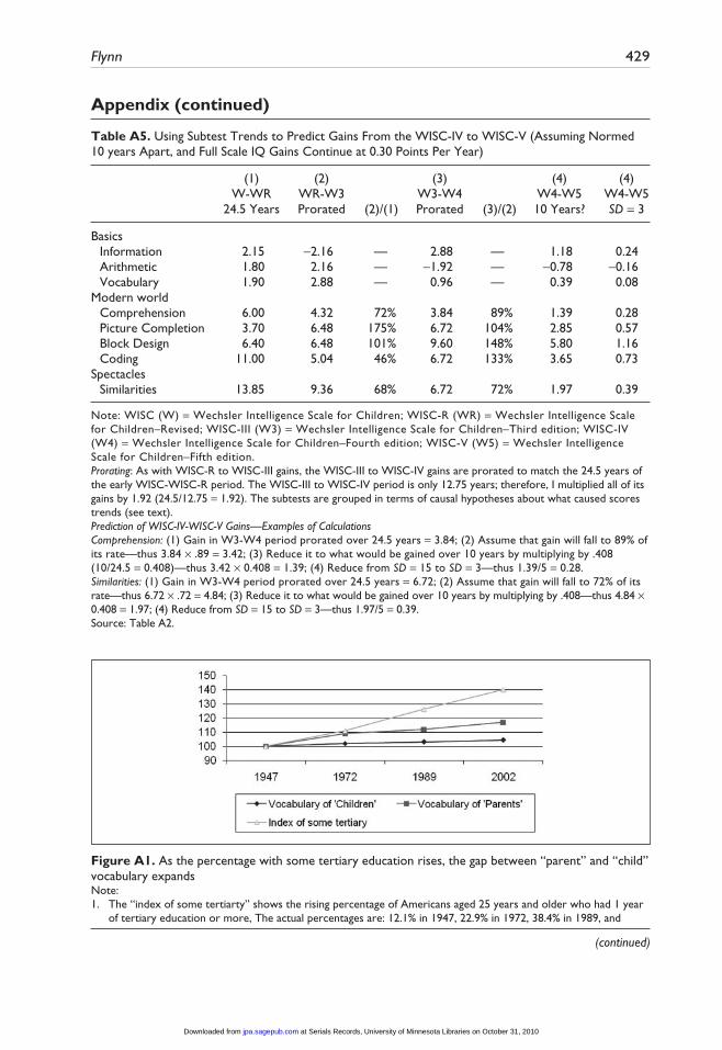
Appendix Table A5 compares what amount to rates of gain over the three WISC periods and uses past trends to predict gains for the WISC-IV to WISC-V period, assuming the WISC-V is normed in 2012. I will divide the subtests into three groups.

Basic subtests that measure skills children needed to cope with school even in 1900. I assume their slow rate of gain will persist. Modern world subtests, whose gains are driven by facets of the modern world independent of the spread of scientific spectacles: partially in the case of Picture Completion and Block Design, wholly for Comprehension and Coding. The average of the predicted



Flynn 421

gains for these four subtests comes to 0.685 (Standard Score points). The spectacles subtest, Similarities, has been in decline throughout the WISC era, and I predict a modest gain of only 0.39 standard score points. Similarities will lose its place as flagship and voyage henceforth as an ordinary member of the fleet.

The decline of both Raven’s and Similarities gains signals the end of an era when the spread of scientific spectacle was the dominant proximate cause of IQ gains. The end of an era does not mean, of course, that it never existed. But from now on, other aspects of the modern world must take up the burden of fueling gains.

The Strange Case of VocabularyComparing WISC and WAIS trends reveals a growing gap between the active vocabularies of U.S. adults and schoolchildren. This was unanticipated. The vocabulary gains of adults should transfer to their children by parent–child interaction. A parent–child gap on Information and Arithmetic subtests differences seemed more plausible. During the second half of the 20th century, American adults have embraced tertiary education, and years of schooling have increased. The tertiary educa-tion gains of adults on Information and Arithmetic would transfer but less efficiently, because they are less prominent in informal parent–child interaction. Interaction is not entirely absent, for example, parents help their children with homework. Nonetheless, children might need to go on to tertiary education themselves to fully benefit. Therefore, there would be a small but detectable gap between adult and child gains on those two subtests.

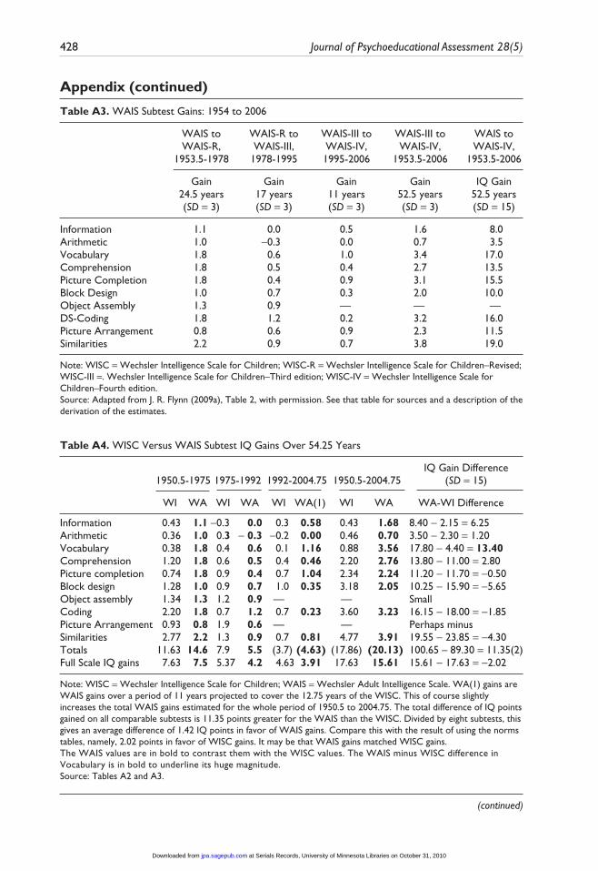
Appendix Table A4 details subtest gains on both the WISC and the WAIS. The object was to compare child and adult gains over much the same periods. Therefore, the beginning and ending dates of the WISC periods and WAIS periods were averaged. The only complication was posed by the final periods of gains. Here the WISC gains represent 12.75 years, and the WAIS gains only 11 years. Therefore, I multiplied WAIS gains by 12.75/11 to get values comparable with the WISC.

Subtest ComparisonsTable 4 summarizes Table A4. It ranks the Wechsler subtests running from where adult gains are larger than child gains to the reverse. Most differences make sense.

Four subtests measure abilities that school may emphasize more than the world of work. These show larger gains for schoolchildren than adults over the 54 years. Coding which measures pro-cessing speed shows a small child surplus of 1.85 points (18.00 − 16.15). Similarities trends show

Table 4. WISC vs. WAIS subtests: Ranked by magnitude of difference between adult and schoolchild gains

Difference in Points (SD = 15) Difference in Percentages

WA − WI = Dif WA/WI = Dif

Vocabulary 17.80 − 4.40 = 13.40 17.80/4.40 = 405Information 8.40 − 2.15 = 6.25 8.40/2.15 = 391Comprehension 13.80 − 11.00 = 2.80 13.80/11.00 = 125Arithmetic 3.50 − 2.30 = 1.20 3.50/2.30 = 152Picture Completion 11.20 − 11.70 = −0.50 11.20/11.70 = 96Coding 16.15 − 18.00 = −1.85 16.15/18.00 = 92Similarities 19.55 − 23.85 = −4.30 19.55/23.85 = 82Block Design 10.25 − 15.90 = −5.65 10.25/15.90 = 64

Note: WA = Wechsler Adult Intelligence Scale; WI = Wechsler Intelligence Scale for Children.Source: Appendix Table A4.




a child surplus of 4.30 points (23.85 − 19.55). But the adult gain is still huge. The shift from utili-tarian thinking to “scientific spectacles” is not something that virtually everyone has achieved by the age of 16. It is a gradual transition toward greater sophistication acquired throughout life. Block Design shows a child surplus of 5.65 points (15.90 − 10.25), which in percentage terms is a large difference. It measures on-the-spot problem-solving skills. Schools have moved toward emphasis on such skills rather than simply the acquisition of socially valued information (Genovese, 2002). The world of work has moved too, but not quite so far. I suspect that these analytic skills do not fully transfer from child to adult because they are partially a response to specific demands that school makes more often than most work. There is a difference in favor of children over adults on Picture Completion, but it is negligible.

Then there are two subtests I thought would show moderate gains in favor of adults. The greater exposure of adults to tertiary education has expanded their store of general information, and some fraction of this would not be transferred from parent to child. Information shows an adult gain surplus of 6.25 points (8.40 − 2.15), larger than expected. Arithmetic shows little gain for anyone: The adult gain over the whole 54.25 years is 3.5 points as compared with a child gain of 2.3 points. This may seem to contradict the Nation’s Report Card (U.S. Department of Education, Institute of Education Sciences, & National Center for Educational Statistics, 2003) that measures mathemati-cal skills over time in children. However, Report Card gains fade away when student face subjects such as Algebra and Geometry that require reasoning rather than mere grasp of the mechanics of calculations (Flynn, 2009b). The last half-century has not enhanced the ability of schoolchildren to reason mathematically. U.S. universities are equally helpless to produce graduates better than the university-deprived adults of the past.

I had no expectations about Comprehension. It has items such as why streets are usually num-bered in consecutive order. It shows a small adult surplus, that is, 2.80 points (13.80 − 11.00). Our society may have enhanced the understanding needed in everyday life better for adults than for children.

Finally, contrary to all expectations, the Vocabulary subtest shows adult gains of 17.80 points and child gains of 4.40 points: a huge adult advantage of 13.40 points. What seems odd is not so much the size of the adult gain, given the spread of tertiary education among adults, but how they can have transferred so little of it to the children they communicate with constantly. The Vocabulary subtest does not measure specialized vocabulary but the language of everyday life.

VocabularyFigure 1 simulates vocabulary gains for “parents” and their own school-age “children.” The match is good in that WAIS samples were tested only 4 to 6 years after WISC samples. Because the WISC children were aged 6 to 16 years, their actual parents would have been 23 to 71 years old. The WAIS comparison sample of 1978 was aged 35 to 44, a somewhat younger age range than the target ages. The later WAIS comparison samples included all adult ages so the match is excellent.

Figure 1 puts the initial “Vocabulary IQ” of both parents and their children in 1947 at 100. As the percentage of Americans 25 years and older with at least 1 year of tertiary education rises, from 12.1% in 1947 to 52.0% in 2002, parents gain at an average rate of 0.324 IQ points per year. As we already know, the children lag behind at a rate of 0.081 points per year. The case for greater exposure to tertiary education looks very strong indeed. However, there is a way of measuring its direct impact on Vocabulary: comparing those aged 16 to 17 years and those 20 to 24 years from the WAIS standardizations samples. The former are almost entirely a pretertiary group, and the latter are either about to graduate or recent graduates.

Table 5 divides these cohorts by IQ level. Leaving the mentally retarded aside as too few to affect population trends, it singles out those at an average Full Scale IQ of 79 as a group that expanded tertiary education would leave largely untouched. It averages the results for those with



Flynn 423

IQs from 121 to 146 as a group among whom the percentage in tertiary education would have increased. At about the end of the 54-year period, the tertiary-influenced scores show a Vocabulary gain (from ages 16-17 to ages 20-24) larger than that of the non–tertiary influenced: Their exposure to tertiary education seems to have given them a bonus equivalent to 3.100 IQ points. However, we are interested in how much that bonus increased over the period and therefore must deduct where it stood in about 1953. With that deduction (0.325), the expansion of tertiary education raised adult “Vocabulary IQ” by 2.775 points.

Thus far, we have ignored the difference between cross-sectional and longitudinal data. The WAIS data compare 20- to 24-year-olds with 16- to 17-year-olds who were their contemporaries

Figure 1. As the percentage with some tertiary education rises, the gap between “parent” and “child” vocabulary expandsNote: For details, see Appendix Figure 1A.

Table 5. Effect of Expanded Tertiary Education on Vocabulary: WAIS to WAIS-IV

Vocabulary Gain From Ages 16-17 to 20-24 (Scaled Scores Points: SD = 3)

WAIS WAIS-III WAIS-IV Average

IQ 1953-1954 1995 2006 WIII and WIV

−2 SD MR 0.00 1.00 0.75 0.875−1 SD (nontertiary) 79 1.75 0.50 0.86 0.680 Median 100 1.69 0.63 0.86 0.745+1 SD (Tertiary) 121 1.80 1.33 1.20 1.265+2 SD (Tertiary) 146 1.83 1.17 1.50 1.335

Difference Tertiary/nontertiary 0.065 0.750 0.490 0.620Converted to IQ pts (SD = 15) 0.325 3.750 2.450 3.100Subtracting WAIS difference — 3.425 2.125 2.775Longitudinal bonus: 17 points/52.5 years = 0.324 per year; × 5 (age 22-17) = 1.620Impact of expansion of tertiary education: 2.775 + 1.620 = 4.395As percentage of total adult gain 1953.5 to 2006: 4.395/ 17.0 = 26%

Note: WA = Wechsler Adult Intelligence Scale; WAIS-III (WIII) = Wechsler Adult Intelligence Scale–Third edition; WAIS-IV (WIV) = Wechsler Adult Intelligence Scale–Fourth edition. Those 1 SD below the median on the Vocabulary subtest have been put at an IQ of 79 (not 85). This is the Full Scale IQ of someone who performs 1 SD below the median on every subtest: I assume that the Vocabulary performance is a typical rather than below-average performance. This also explains the values of 121 and 146.Source: Wechsler, 1955, pp. 101-103; Wechsler, 1981, pp. 142-144; Wechsler, 1997, pp. 181-184; Wechsler, 2008, pp. 206-208.




and not with themselves as 17-year-olds some 5 years earlier. During those 5 years, the vocabular-ies of 17-year-olds might have expanded, so we would have an underestimate of the personal gain from tertiary education. Table 5 assumes that the 5 years in question were typical of the whole 52.5-year period and compensates by an extra 1.62 points. This raises the total benefit from tertiary education to almost 4.4 points, which makes tertiary education responsible for 26% of the total gain (4.4/17 = 0.26).

This is a rough estimate. Other factors may have differentiated high-IQ and low-IQ Americans progressively over the past 50 years, such as incarceration rates and addiction. On the other hand, tertiary education has played an indirect role. Its expansion was a prerequisite for a new world of work in which far more people filled vocabulary-demanding jobs as professionals, managers, and technicians. Still, direct credit for the larger part of adult vocabulary gains must go to the work years rather than to the college years.

Active Versus Passive VocabularyThe General Social Survey (GSS; 2009) administered a vocabulary test to a representative sample of English-speaking adult Americans from 1978 through 2006. These correspond to the years in which the WAIS-R and WAIS-IV standardization samples were tested.

Table 6 presents the 1978 and 2006 curves on the GSS Vocabulary test at four performance levels and compares these in terms of their distance above or below the mean. Averaging the four comparisons shows that the 2006 sample was superior by 0.125 SDs or 1.88 IQ points. This falls well short of the gain that WAIS samples registered over those 28 years. Appendix Table A3 puts the latter at 8.00 points (SS gains of 0.6 + 1.0 = 1.6 and 1.6 × 5 = IQ gain of 8.00). Three possible explanations follow.

Sampling. The obvious explanation is almost certainly false. I have placed the WAIS Full Scales IQ gains in the context of a matrix of 14 comparisons (Appendix Table A6). The bottom of the table tells how to calculate the eccentricity of the norms of a particular test. The values indicate that my estimate of Full Scale IQ gains for the relevant period may be 0.415 points too high (0.420 − 0.005). For the whole period from the WAIS to the WAIS-IV, my estimate may be 0.105 points too low (0.10 + 0.005). Zhou et al. (2010) think the use of the matrix in this way is bad science (see the appendix for full discussion).

The WAIS data afford good estimates of Full Scale IQ gains, that is, gains based on the col-lection of all 10 subtests. Perhaps the WAIS samples consisted of subjects whose performances were representative on all subtests except Vocabulary? No random error would produce such a result, namely, people who were somewhat above average for vocabulary (but average for every-thing else) in 1978, more above average for Vocabulary (and it alone) in 1995, and more still above average for Vocabulary (and it alone) in 2006. You would have to deliberately oversample the preparers of dictionaries and gradually increase their overrepresentation over time.

Table 6. General Social Survey: Vocabulary Gains 1978 to 2006

Items SDs Above or SDs above or Difference Correct 1978% Below Mean 2006% below mean favoring 2006 IQ points

0 to 4 24.4 0.694 B 18.3 0.904 B 0.210 3.150 to 5 40.3 0.246 B 35.5 0.372 B 0.126 1.890 to 6 60.9 0.277 A 56.5 0.164 A 0.113 1.700 to 7 76.6 0.726 A 75.0 0.674 A 0.052 0.78

Note: Average of comparisons: 1.88 IQ points (0.125 SDs). Compensation for obsolete item (average ignoring top-scoring group): 2.25 points. WAIS gains 1978 to 2006: 8.00 IQ pointsSource: General Social Surveys, 2009 (Cumulative File for wordsum 1972-2006).



Flynn 425

Test content. The GSS vocabulary test has used the same 10 words since its inception in 1972. Was the 2006 GSS sample handicapped by semiobsolete words? One word of the 10 looks a bit dated. I cannot name it, but it would be as if today’s adults were presented with a word like “not-withstanding.” The 2006 sample outperforms the 1972 sample at all levels right up to getting a really high score (8-10 items correct), as if its best members were finding one item unusually dif-ficult. However, when Table 6 compensates by ignoring the top of the curves, the GSS gain rises to only 2.25 points, still well short of the WAIS 8.0-point gain. It is possible, of course, that gains were less among high-IQ subjects, but I wish to be conservative (for reasons that will become apparent) about a mismatch between GSS and WAIS results.

Test format. The WAIS is a “free recall paradigm” requiring the subject to volunteer the mean-ing of the words read out. The GSS is a “recognition paradigm.” It offers five possible synonyms, and the subject must recognize the one that is correct. If we assume that the WAIS and GSS results do not differ because of sampling error, it must be because the former is testing active vocabulary rather than passive. That is, the WAIS discovers what words people are likely to actually use in conversation or composition, whereas the GSS discovers what words people are likely to under-stand in context, if someone else uses them or if they read them in a book.

Initially, it may seem impossible that, from 1978 to 2006, American adults would gain 8.00 points for active vocabulary and 2.25 points for passive. The latter is only 28% of the former. However, recall and recognition involve different brain structures and processes. It is not uncom-mon for individuals with traumatic brain injury to be able to recognize a correct answer that they cannot recall. During half a century, if the worlds of college and work altered their verbal demands toward the capacity to actually use more words, the appropriate brain structures would become more developed, just as if we all began to swim a lot, our muscles would adapt. No physiological impediment bars a greater increase of active than passive vocabulary over time.

The data suggest this summary for the whole period from 1950 to 2004: American schoolchil-dren gained 4.4 points for active vocabulary, American adults gained 17.8 points for active vocabu-lary, American adults made a much lower gain for passive vocabulary—assuming it was 28% of the active for the whole period, it would have been about 5 points (0.28 × 17.8). We do not know what passive gain children made. Even if they made none, they did not fall far behind adults. We can now restate our central problem: Why do parents and the children they raise show a widening gap in their vocabularies; why has the active vocabulary gap become wider than the passive gap? The active gap (13.4 points) puts school children at the 18th percentile on the adult curve; the maximum passive gap (4.98 points) puts them at the 37th percentile.

Parents Talking to TeenagersAround 1950, when parents addressed their teenage children, the latter understood them and answered in kind. Today, their children understand them reasonably well. But to a significant degree, they cannot answer in kind or use their parent’s vocabulary when talking to their peers or anyone from the adult world. The trend is nullified as children become adults. The tertiary years weigh in, and then the world of work finishes the job of turning the teenage-speak teenager into an adult-speak adult. So the long-term social consequences are not serious. Even when adults lecture to freshmen at university, students will understand their speech even if they cannot, at that point in their lives, imitate it.

Mintz (2004) asserts that teenage subculture did not exist until 1950. Most young people aspired to adulthood as fast as their physical development allowed. Despite debate about this, most agree on certain brutal facts: It is an increasingly autonomous subculture that has acquired its own dress, hairstyles, music, income for consumption, and dialect. WAIS versus WISC trends since 1950




suggest that teenage subculture has evolved. It always had the power to make its members use an alternative to adult speech. Today it inhibits them from developing the capacity to use adult speech. They have become less bilingual and more monolingual.

Celtic nationalities in the British Isles that resent an “alien” language try to revive their tradi-tional language. Teenagers have not only created an alternative dialect but also withdrawn from their natural speech community. Until recently, U.S. adults did not expect to bear the burdens of parenting beyond the age of 15 years. Perhaps antagonism between parents and teenager rises as dependence is prolonged. Perhaps parents have begun to impose goals (e.g., get into Harvard) most teenagers cannot attain. Cognitive trends over time are not events that happen in a test room: They signal the existence of important social trends.

Tribute to KaufmanMy book What Is Intelligence? Beyond the Flynn Effect (Flynn, 2009b) solves some of the para-doxes posed by massive IQ gains over time. But nothing would be worse than people sitting around admiring my “theory.” Imitate Kaufman, and bombard it with every objection you can. That is how science progresses.

Appendix

Table A1. WISC to WISC-R: Score Differences Revealed by Uniform Scoring

Studies N WISC WISC-R WISC-R-III Difference

Solly (1977) 12 136.08 123.67 122.94 13.14Larrabee and Holroyd (1976) 38 132.00 122.60 121.79 10.21Tuma et al. (1978) 18 127.60 124.70 124.04 3.56Wheaton et al. (1980) 50 127.24 122.84 122.05 5.19Appelbaum and Tuma (1977) 20 125.21 123.42 122.67 2.54Schwarting (1976) 58 113.40 105.91 103.91 9.49Rowe (1977) 128 109.92 103.30 101.11 8.81Stokes et al. (1978) 59 109.83 107.32 105.42 4.41Davis (1977) 54 107.45 99.80 97.36 10.09

Summary Group IIIA (counterbalanced): Average WISC IQ = 116.11, Average gain = 7.79

Klinge, Rodziewicz, and Schwartz (1976) 32 98.72 95.33 92.57 6.15Applebaum and Tuma (1977) 20 98.25 94.30 91.47 6.78Brooks (1977) 30 96.40 89.17 85.48 10.42Tuma et al. (1978) 18 96.20 91.00 87.94 8.26Munford (1978) 20 92.50 87.50 84.19 8.31Swerdick (1978) 164 91.33 85.86 82.43 8.90Hartlage and Boone (1977) 42 90.93 85.86 82.43 8.50Weiner and Kaufman (1979) 46 89.70 81.70 77.97 11.73Covin (1977) 30 89.33 89.40 86.22 3.11

Summary Group IIIB (counterbalanced): Average WISC IQ = 92.54, Average gain = 8.48

I. Solway et al. (1976) 180 84.74 79.57 75.69 9.05I. Thomas (1980) 93 80.97* 75.85 71.70 9.27II. Reschly and Davis (1977) 48 76.65 73.04 68.24* 8.41II. Covin (1976) 101 76.63 74.00 69.12* 7.51I. Udziela and Barclay (1893) 45 66.79 64.80 59.86 6.93I. Catron and Catron (1977) 29 65.30 59.66 54.36 10.94

(continued)



Flynn 427

II. Gironda (1977) 20 63.90 64.00 58.11* 5.79II. Spitz (1983) 33 61.42 56.30 50.07* 11.35

Summary Group I + II (non-counterbalanced): Average WISC IQ = 77.24, Average gain = 8.13

Reynolds and Hartlage (1979) 66 84.06 79.41 75.52 8.54Sherrets and Quattrocchi (1979) 28 78.43 75.00 70.79 7.64Rowe (1977) 22 76.39 74.85 70.63 5.76Solly (1977) 12 76.25 65.42 60.63 15.72Hamm et al. (1976) 48 70.41 62.85 59.65* 10.76McGinley (1981) 21 68.05 61.57 57.04* 11.01

Summary Group IIIC (counterbalanced): Average WISC IQ = 76.89, Average gain = 9.34

Rowe (1977; counterbalanced) 22 56.23 48.79 42.71 13.52

Summary Group IIID (counterbalanced): Average WISC IQ = 56.23, Average gain = 13.52

All non-counterbalanced 549 Gain = 8.13All counterbalanced 1058 Gain = 8.46All studies 1607 Gain = 8.35

Note: WISC = Wechsler Intelligence Scale for Children; WISC-R = Wechsler Intelligence Scale for Children–Revised; WISC-R-III = Wechsler Intelligence Scale for Children–Revised (Third edition). All averages are weighted averages. As the table shows, including the counterbalanced studies increased the estimate of IQ gains by only 0.22 IQ points (8.35 − 8.13). Scores marked with an asterisk were adjusted slightly (see Flynn, 1985). Classification system: I—Marks three studies where subjects were assigned to take either the WISC or WISC-R randomly and one in which two groups who took the WISC-R later were matched for WISC IQs. II—Marks four studies where subjects took the WISC-R some 1.5 to 3.0 years after the WISC. III—All studies counterbalanced but subdivided by IQ level from above average (IIIA), to low average (IIIB), to low IQ (IIIC), to very low IQ (IIID).Source: Adapted from Flynn, 1985, Table 1, with permission of the American Psychological Association. The references for all studies listed are there.

Table A2. WISC Subtest Gains: 1947 to 2002

WISC to WISC-R to WISC-III to WISC to WISC to WISC-R, WISC-III, WISC-IV, WISC-IV, WISC-IV, 1947.5-1972 1972-1989 1989-2001.75 1947.5-2001.75 1947.5-2001.75

Gain Gain Gain Gain IQ Gain 24.5 years 17 years 12.75 years 54.25 years 54.25 years (SD = 3) (SD = 3) (SD = 3) (SD = 3) (SD = 15)

Information 0.43 −0.3 0.3 0.43 2.15Arithmetic 0.36 0.3 −0.2 0.46 2.30Vocabulary 0.38 0.4 0.1 0.88 4.40Comprehension 1.20 0.6 0.4 2.20 11.00Picture Completion 0.74 0.9 0.7 2.34 11.70Block Design 1.28 0.9 1.0 3.18 15.90Object Assembly 1.34 1.2 [0.93] [3.47] [17.35]Coding 2.20 0.7 0.7 3.60 18.00Picture Arrangement 0.93 1.9 [1.47] [4.30] [21.50]Similarities 2.77 1.3 0.7 4.77 23.85

Note: WISC = Wechsler Intelligence Scale for Children; WISC-R = Wechsler Intelligence Scale for Children–Revised; WISC-III = Wechsler Intelligence Scale for Children–Third edition; WISC-IV = Wechsler Intelligence Scale for Children–Fourth edition.Source: Adapted from J. R. Flynn, What Is intelligence? Beyond the Flynn Effect [Enlarged Paperback Edition], Cambridge University Press, 2009, Table 1, with permission of the Syndics of the Cambridge University Press. See that table for sources and a description of the derivation of the estimates.

(continued)

Appendix (continued)




Table A3. WAIS Subtest Gains: 1954 to 2006

WAIS to WAIS-R to WAIS-III to WAIS-III to WAIS to WAIS-R, WAIS-III, WAIS-IV, WAIS-IV, WAIS-IV, 1953.5-1978 1978-1995 1995-2006 1953.5-2006 1953.5-2006

Gain Gain Gain Gain IQ Gain 24.5 years 17 years 11 years 52.5 years 52.5 years (SD = 3) (SD = 3) (SD = 3) (SD = 3) (SD = 15)

Information 1.1 0.0 0.5 1.6 8.0Arithmetic 1.0 −0.3 0.0 0.7 3.5Vocabulary 1.8 0.6 1.0 3.4 17.0Comprehension 1.8 0.5 0.4 2.7 13.5Picture Completion 1.8 0.4 0.9 3.1 15.5Block Design 1.0 0.7 0.3 2.0 10.0Object Assembly 1.3 0.9 — — —DS-Coding 1.8 1.2 0.2 3.2 16.0Picture Arrangement 0.8 0.6 0.9 2.3 11.5Similarities 2.2 0.9 0.7 3.8 19.0

Note: WISC = Wechsler Intelligence Scale for Children; WISC-R = Wechsler Intelligence Scale for Children–Revised; WISC-III =. Wechsler Intelligence Scale for Children–Third edition; WISC-IV = Wechsler Intelligence Scale for Children–Fourth edition.Source: Adapted from J. R. Flynn (2009a), Table 2, with permission. See that table for sources and a description of the derivation of the estimates.

Table A4. WISC Versus WAIS Subtest IQ Gains Over 54.25 Years

IQ Gain Difference 1950.5-1975 1975-1992 1992-2004.75 1950.5-2004.75 (SD = 15)

WI WA WI WA WI WA(1) WI WA WA-WI Difference

Information 0.43 1.1 −0.3 0.0 0.3 0.58 0.43 1.68 8.40 − 2.15 = 6.25Arithmetic 0.36 1.0 0.3 − 0.3 −0.2 0.00 0.46 0.70 3.50 − 2.30 = 1.20Vocabulary 0.38 1.8 0.4 0.6 0.1 1.16 0.88 3.56 17.80 − 4.40 = 13.40 Comprehension 1.20 1.8 0.6 0.5 0.4 0.46 2.20 2.76 13.80 − 11.00 = 2.80Picture completion 0.74 1.8 0.9 0.4 0.7 1.04 2.34 2.24 11.20 − 11.70 = −0.50Block design 1.28 1.0 0.9 0.7 1.0 0.35 3.18 2.05 10.25 − 15.90 = −5.65 Object assembly 1.34 1.3 1.2 0.9 — — SmallCoding 2.20 1.8 0.7 1.2 0.7 0.23 3.60 3.23 16.15 − 18.00 = −1.85Picture Arrangement 0.93 0.8 1.9 0.6 — — Perhaps minusSimilarities 2.77 2.2 1.3 0.9 0.7 0.81 4.77 3.91 19.55 − 23.85 = −4.30Totals 11.63 14.6 7.9 5.5 (3.7) (4.63) (17.86) (20.13) 100.65 – 89.30 = 11.35(2) Full Scale IQ gains 7.63 7.5 5.37 4.2 4.63 3.91 17.63 15.61 15.61 − 17.63 = −2.02

Note: WISC = Wechsler Intelligence Scale for Children; WAIS = Wechsler Adult Intelligence Scale. WA(1) gains are WAIS gains over a period of 11 years projected to cover the 12.75 years of the WISC. This of course slightly increases the total WAIS gains estimated for the whole period of 1950.5 to 2004.75. The total difference of IQ points gained on all comparable subtests is 11.35 points greater for the WAIS than the WISC. Divided by eight subtests, this gives an average difference of 1.42 IQ points in favor of WAIS gains. Compare this with the result of using the norms tables, namely, 2.02 points in favor of WISC gains. It may be that WAIS gains matched WISC gains.The WAIS values are in bold to contrast them with the WISC values. The WAIS minus WISC difference in Vocabulary is in bold to underline its huge magnitude.Source: Tables A2 and A3.

(continued)




Flynn 429

Table A5. Using Subtest Trends to Predict Gains From the WISC-IV to WISC-V (Assuming Normed 10 years Apart, and Full Scale IQ Gains Continue at 0.30 Points Per Year)

(1) (2) (3) (4) (4) W-WR WR-W3 W3-W4 W4-W5 W4-W5 24.5 Years Prorated (2)/(1) Prorated (3)/(2) 10 Years? SD = 3

Basics Information 2.15 −2.16 — 2.88 — 1.18 0.24Arithmetic 1.80 2.16 — −1.92 — −0.78 −0.16Vocabulary 1.90 2.88 — 0.96 — 0.39 0.08

Modern world Comprehension 6.00 4.32 72% 3.84 89% 1.39 0.28Picture Completion 3.70 6.48 175% 6.72 104% 2.85 0.57Block Design 6.40 6.48 101% 9.60 148% 5.80 1.16Coding 11.00 5.04 46% 6.72 133% 3.65 0.73

Spectacles Similarities 13.85 9.36 68% 6.72 72% 1.97 0.39

Note: WISC (W) = Wechsler Intelligence Scale for Children; WISC-R (WR) = Wechsler Intelligence Scale for Children–Revised; WISC-III (W3) = Wechsler Intelligence Scale for Children–Third edition; WISC-IV (W4) = Wechsler Intelligence Scale for Children–Fourth edition; WISC-V (W5) = Wechsler Intelligence Scale for Children–Fifth edition.Prorating: As with WISC-R to WISC-III gains, the WISC-III to WISC-IV gains are prorated to match the 24.5 years of the early WISC-WISC-R period. The WISC-III to WISC-IV period is only 12.75 years; therefore, I multiplied all of its gains by 1.92 (24.5/12.75 = 1.92). The subtests are grouped in terms of causal hypotheses about what caused scores trends (see text).Prediction of WISC-IV-WISC-V Gains—Examples of CalculationsComprehension: (1) Gain in W3-W4 period prorated over 24.5 years = 3.84; (2) Assume that gain will fall to 89% of its rate—thus 3.84 × .89 = 3.42; (3) Reduce it to what would be gained over 10 years by multiplying by .408 (10/24.5 = 0.408)—thus 3.42 × 0.408 = 1.39; (4) Reduce from SD = 15 to SD = 3—thus 1.39/5 = 0.28.Similarities: (1) Gain in W3-W4 period prorated over 24.5 years = 6.72; (2) Assume that gain will fall to 72% of its rate—thus 6.72 × .72 = 4.84; (3) Reduce it to what would be gained over 10 years by multiplying by .408—thus 4.84 × 0.408 = 1.97; (4) Reduce from SD = 15 to SD = 3—thus 1.97/5 = 0.39.Source: Table A2.


Figure A1. As the percentage with some tertiary education rises, the gap between “parent” and “child” vocabulary expandsNote:1. The “index of some tertiarty” shows the rising percentage of Americans aged 25 years and older who had 1 year

of tertiary education or more, The actual percentages are: 12.1% in 1947, 22.9% in 1972, 38.4% in 1989, and

(continued)




52.0% in 2002 (Bureau of Labor Statistics & U.S. Census Bureau, 1940-2007). The slope was contrived simply to show a rise in the percentage with some teriarary education about double the vocabulary gain for adults over the same period. It has no more justification than the fact that the correlation between the two cannot be perfect.

2. The rationale of referring to WAIS vocabulary gains as the gains of “parents” and the WISC vocabulary gains as the gains of “their children” is described in the text.

3. Note that the years refer to when WISC standardization sample were tested. However, the number of years between testings was the same for the WISC and WAIS except during the last period. In it, there were 12.75 years between when the WISC-III and WISC-IV samples were tested but only 11 years between when the WAIS-III and WAIS-IV samples were tested. If the WAIS gain in that last period were multiplied by 12.75/11, it would be increased by 0.80 points (5 × 12.75/11 = 5.80). That would increase the widening gap between adult and schoolchild vocabulary gains from 12.6 IQ points (17.0 − 4.4) to 13.4 points (17.8 − 4.4). This adjustment was done in Table A4 but has not been done here.

4. The IQ gains are from Table A2 and Table A3.

Table A6. Fourteen Estimates of Recent IQ Gains Over Time

Ideal Period Ideal Versus Tests Compared Gains Years Rate Gain Real

(1) WAIS-III (1995) and SB-5 (2001) +5.50 6 +0.917 1.80 3.70(2) WAIS-R (1978) and SB-4 (1985) +3.42 7 +0.489 2.10 1.32(3) WAIS-III (1995) and WISC-IV (2001.75) +3.10 6.75 +0.459 2.03 1.07(4) WISC-III (1989) and SB-5 (2001) +5.00 12 +0.417 3.60 1.40(5) WISC-III (1989) and +4.23 12.75 +0.332 3.83 0.40

WISC-IV (2001.75)(6) WISC-R (1972) and +5.30 17 +0.312 5.10 0.20

WISC-III (1989)(7) WISC-R (1972) and SB-4 (1985) +2.95 13 +0.227 3.90 0.95(8) SB-4 (1885) and SB-5 (2001) +2.77 16 +0.173 4.80 2.03(9) WAIS-R (1978) and WAIS-III (1995) +4.20 17 +0.247 5.10 0.90(10) SB-LM (1972) and SB-4 (1985) +2.16 13 +0.166 3.90 1.74(11) WISC-R (1972) and WAIS-R (1978) +0.90 6 +0.150 1.80 0.90(12) WISC-III (1989) and WAIS-III (1995) −0.70 6 −0.117 1.80 2.50(13) WAIS-III (1995) and WAIS-IV (2006) +3.37 11 +0.306 3.30 0.07(14) WISC-IV (2001.75) and WAIS-IV (2006) +1.20 4.25 +0.282 1.28 0.08Average of all 14 comparisons +0.311 1.23Average of 4 WISC/WISC +0.299 0.39 and WAIS/WAIS comparisons

Note: WAIS = Wechsler Adult Intelligence Scale; WAIS-R = Wechsler Adult Intelligence Scale–Revised; WAIS-III = Wechsler Adult Intelligence Scale–Third edition; WAIS-IV = Wechsler Adult Intelligence Scale–Fourth edition; WISC-R (WR) = Wechsler Intelligence Scale for Children–Revised; WISC-III (W3) = Wechsler Intelligence Scale for Children–Third edition; WISC-IV (W4) = Wechsler Intelligence Scale for Children–Fourth edition; SB = Stanford–Binet; SB-LM = Stanford–Binet Form L-M. This table allows an assessment of whether the norms of a given test seem eccentric. For example, if a test has substandard norms, it will inflate estimates when paired with a later test and deflate estimates when paired with an earlier test. Using the Ideal versus Real column to test Wechsler adult tests (+ = inflated IQs, − = deflated IQs): WAIS-R pairs: (2) +1.32 points, (9) −0.90, (11) +0.90. Average = +0.42. WAIS-III pairs: (1) +3.70, (3) +1.07, (13) +0.07, (9) +0.90, (12) +2.50. Average = +1.65. WAIS IV pairs: (13) −0.07, (14) +0.08. Average = +0.005. Flynn (1984b), Table 2, allows the same assessment of the WAIS. WAIS pairs: (4) −1.09, (5) −0.88, (9) +0.41, (10) −0.84, (14) +1.10, (15) +0.69. Average = −0.102.Comparisons of like with like, either comparisons of two versions of the WISC or two versions of the WAIS, are in bold.


(continued)



Flynn 431

Postscript for the Psychological Corporation

Does using the matrix (Table A6) lead, as Zhou et al. (2010) claim, to bad science? A review of my thinking over the years may convince them that things are not that bad, and that they could be more charitable.

1. The bone of contention was using the matrix to question the norms of the WAIS-III. Up to 2006, it seemed that the WAIS-III behaved as follows: When it was the earlier test of a pair, it gave IQ gains at the rate of 0.668 points per year; when it was the later test, it gave only 0.027 (Flynn, 2009b). This was radically out of step with WISC data, which consis-tently gave just greater than 0.300 points per year. As I pointed out, positing that the WAIS-III norms were too weak by 2.34 points eliminated the discrepancies the matrix revealed.

2. There is nothing unusual about this in the history of science. Often when an observation is at variance with a well-attested uniformity, the hypothesis of measurement error is given. What if the WAIS-III had show no gains or even a negative value whenever it was the later test in a pair? The value of 0.027 was close enough to zero to arouse suspicion. It is a judgment call, but I believe anyone would have been suspicious for whom the WAIS-III was not a favorite child.

This is particularly true when the observation in question is made under conditions when measurement error is likely. I granted that it was logically possible that adults would show eccentricities in the continuity of their rate of gain absent in children. But in support of my hypothesis, I pointed out the difficulties of getting representative samples of adults (WAIS) as opposed to children (WISC). If you get a good stratified sample of schools, the children are captive subjects. Adults have to be got either at work or at home which makes sampling far more difficult.

3. The index of good or bad science is whether you are willing to test a hypothesis against evidence. Mine generated two predictions.

4. First prediction: When the WAIS-IV appeared, gains measured using the WAIS-III and WAIS-IV should be inflated. After all, the WAIS-III is the earlier test in this pair. Yet when the matrix was updated (Flynn, 2009a, Table 1), these gains proved entirely typical at 0.306 points per year. Moreover, I had revised my estimate of WAIS-R to WAIS-III gains using the more accurate method Flynn and Weiss applied to the WISC-III and WISC-IV combination. This now showed gains at the rate of 0.247 points per year for the WAIS-R to WAIS-III combination. Now one had to assume that the WAIS-III norms were too weak by only 1.65 points to eliminate all discrepancies in the matrix. Even more significant, if you confined yourself to WAIS data, a corrective of only 0.49 points was sufficient. As I said (Flynn, 2009a), I was about to exonerate the WAIS-III from the charge that its standardization sample was substandard.

5. Second prediction: Other relatable IQ tests would cast doubt on the WAIS-III norms. Unlike the first prediction, the second began to be confirmed with a vengeance. Floyd, Clark, and Shadish (2008) showed that a group of 148 college undergraduates scored 8.64 points higher (adjusted for dates of standardization) on the WAIS-III than on the Woodcock–Johnson III, and a group of 99 subjects scored 6.77 points higher (adjusted) than on the Kaufman Adolescent and Adult Intelligence Scale. This was deeply disturb-ing. I urged that in capital cases, WAIS-III scores should be set aside and the defendant tested anew on both the WAIS-IV and the Stanford–Binet 5.


(continued)




6. In summary, the matrix is meant not to reach dogmatic conclusions (which would indeed be bad science). It is meant to pose hypotheses to be tested against evidence. I hope I have shown a willingness to do just that. It would also be bad science to be dogmatically convinced that adult samples can be impeccably representative, and I assume that Zhou et al. (2010) are not so remiss. So let us put some hypotheses to the test. I have two sug-gestions that as scientists, Zhou et al. and I and everyone else can adopt.

Proposed Research Design IThe Psychological Corporation could use its excellent method of sample selection to norm the WAIS-V. At the same time, the Woodcock–Johnson organization would use its excellent method to select a sample of adults and use them to norm WAIS-V. I predict a discrepancy between the two sets of norms amounting to one or two points.

Proposed Research Design II1. Collect 1,000 extra subjects for the WISC-V standardization sample.2. Give them the WISC only.

Then we would know what gains had occurred between 1947-48 and 2012, not only for Full Scale IQ but also for all subtests, without any complications.

I am no good at raising money but I bet that if the Psychological Corporation (and the American Psychological Association) back such proposals, the money will be found.

Declaration of Conflicting Interests

The author(s) declared no potential conflicts of interest with respect to the authorship and/or publication of this article.

Funding

The author(s) received no financial support for the research and/or authorship of this article.

References

Bureau of Labor Statistics & U.S. Census Bureau. (1940-2007). Current population surveys (1940-2007). Table A-1. Years of school completed by people 25 years and over, by age and sex (selected years). Washington, DC: Author.

Daley, T. C., Whaley, S. E., Sigman, M. D., Espinosa, M. P., & Neumann, C. (2003). IQ on the rise: The Flynn effect in rural Kenyan children. Psychological Science, 14, 215-219.

Davis, E. E. (1977). Matched pair comparison of WISC and WISC-R scores. Psychology in the Schools, 14, 161-166.

Floyd, R. G., Clark, M. H., & Shadish, W. R. (2008). The exchangeability of IQs: Implications for profes-sional psychology. Professional Psychology: Research and Practice, 39, 4514-4523.

Flynn, J. R. (1984a). IQ gains and the Binet decrements. Journal of Educational Measurement, 21, 283-290.Flynn, J. R. (1984b). The mean IQ of Americans: Massive gains 1932 to 1978. Psychological Bulletin, 95,

29-51.Flynn, J. R. (1985). Wechsler intelligence tests: Do we really have a criterion of mental retardation?

American Journal of Mental Deficiency, 90, 236-244.




Flynn 433

Flynn, J. R. (1987). Massive IQ gains in 14 nations: What IQ tests really measure. Psychological Bulletin, 101, 171-191.

Flynn, J. R. (1998). IQ gains over time: Towards finding the causes. In U. Neisser (Ed.), The rising curve: long term gains in IQ and related measures (pp. 25-66). Washington, DC: American Psychological Association.

Flynn, J. R. (2009a). The WAIS-III and WAIS-IV: Daubert motions favor the certainly false over the approximately true. Applied Neuropsychology, 16, 1-7.

Flynn, J. R. (2009b). What is intelligence? Beyond the Flynn Effect (Expanded paperback ed.). Cambridge, England: Cambridge University Press.

Flynn, J. R., & Rossi-Casé, L. (2010). IQ gains in Argentina between 1964 and 1998. Manuscript submitted for publication.

General Social Surveys. (2009). Cumulative file for wordsum 1972-2006. Chicago, IL: National Opinion Research Center.

Genovese, J. E. (2002). Cognitive skills valued by educators: Historic content analysis of testing in Ohio. Journal of Educational Research, 96, 101-114.

Haselbauer, N. (2009). The mammoth book of quick puzzles. London, England: Constable & Robinson.Jensen, A. R. (1980). Bias in mental testing. London, England: Methuen.Kaufman, A. S. (2003). Practice effects. Clinical Café Archive, October.Kaufman, A. S. (2010). “In what way are apples and oranges alike?” A critique of Flynn’s interpretation of

the Flynn effect. Journal of Psychoeducational Assessment, 28, 382-398.Klinge, V., Rodziewicz, T., & Schwartz, L. (1976). Comparison of the WISC and WISC-R on a psychiatric

adolescent inpatient sample. Journal of Abnormal Psychology, 4, 73-81.Larrabee, G. J., & Holyroyd, R. G. (1976). Comparison of WISC and WISC-R using a sample of highly

intelligent students. Psychological Reports, 38, 1071-1074.Mensa (2006). Mensa boost your IQ. London, England: Carlton Books.Mintz, S. (2004). Huck’s raft: A history of American childhood. Cambridge, MA: Harvard University Press.Munford, P. R. (1978). A comparison of the WISC and WISC-R on black child psychiatric outpatients.

Journal of Clinical Psychology, 34, 938-943.Rowe, H. A. H. (1977). “Borderline” versus “mentally deficient.” Australian Journal of Mental Retardation,

4, 11-14.Sherrets, S., & Quattrocchi, M. (1979). WISC—WISC-R differences—fact or artifact? Journal of Pediatric

Psychology, 4, 119-127.U.S. Department of Education, Institute of Education Sciences, & National Center for Educational Statistics.

(2003). The nation’s report card: Reading 2002, NCES 2003-521, by W. S. Grigg, M. C. Daane, Y. Jin, and J. R. Campbell. Washington, DC: Author.

Wechsler, D. (1955). Wechsler Adult Intelligence Scale: Manual. New York, NY: Psychological Corporation.Wechsler, D. (1981). Wechsler Adult Intelligence Scale–Revised: Manual. New York, NY: Psychological

Corporation.Wechsler, D. (1997). Wechsler Adult Intelligence Scale–Third edition: Manual. San Antonio, TX: Psycho-

logical Corporation.Wechsler, D. (2008). Wechsler Adult Intelligence Scale–Fourth edition: Manual. San Antonio, TX: Pearson.Zhou, X., Zhu, J., & Weiss, L. G. (2010). Peeking inside the “black box” of the Flynn effect: Evidence from

three Wechsler instruments. Journal of Psychoeducational Assessment, 28, 399-411.



Documents

2010b - Institute for Applied Psychometrics (IAP)