CONTENTSgc.nuaa.edu.cn/hangkong/doc/ziliao/MSC_PATRAN/MS… · · 2009-05-31MSC.Laminate Modeler Integration with MSC.Patran, 4 ... Create LM_Material Add Form, 45 ... are then

C O N T E N T SMSC.Laminate Modeler User’s Guide MSC.Laminate Modeler User’s

Guide

CHAPTER

1Overview ■ Purpose, 2

■ MSC.Laminate Modeler Product Information, 3

■ What is Included with this Product?, 3

■ MSC.Laminate Modeler Integration with MSC.Patran, 4

■ What is MSC.Laminate Modeler?, 5

2Tutorial ■ Introduction, 8

■ Composite Materials and Manufacturing Processes, 9❑ Composite Materials, 9❑ Common Material Forms, 9❑ Common Manufacturing Forms, 10

■ Composites Design, Analysis and Manufacture, 12❑ The Development Process, 12❑ Requirements of CAE Tools for Composites Development, 12❑ Composites Development Within the MSC.Patran Environment, 16

■ Draping Simulation (Developable Surfaces), 17❑ Definition of Developable Surfaces, 17❑ Example of Waffle Plate, 18❑ Benefits of MSC.Laminate Modeler, 19

■ Draping Simulation (Non-Developable Surfaces), 20❑ Definition of Non-Developable Surfaces, 20❑ Benefits of MSC.Laminate Modeler, 24

■ Building Models using Global Layers, 25❑ Global Layer Description of Layup, 25❑ Example of a Top Hat Section, 26❑ Benefits of MSC.Laminate Modeler, 28

■ Results Processing, 29❑ Recovering Results by Global Layer, 29❑ Example of a Top Hat Section, 29❑ Benefits of MSC.Laminate Modeler, 31

■ Structural Optimization, 32❑ Introducing Iteration to the Development Process, 32❑ Example of a Torque Tube with a Cutout, 32❑ Benefits of MSC.Laminate Modeler, 34

■ Glossary, 35

3Using MSC.Laminate Modeler

■ Procedure, 38

■ Element Library, 40❑ Supported Element Topologies, 40❑ Supported Element Types, 41❑ Supported Element Property Words, 41

■ Initialization, 42

■ Creating Materials, 43❑ Create LM_Material Add Form, 45❑ Modify LM_Material Form, 46❑ Show LM_Material Form, 47❑ Delete LM_Material Select Form, 48

■ Creating Plies, 49❑ Create LM_Ply Add Form (Draping), 50

- Input Data Definitions, 51- Additional Controls Form - Geometry, 55- Additional Controls Form - Material, 56- Additional Controls Form - Boundaries, 57- Additional Controls Form - Order of Draping, 58

❑ Create LM_Ply Add Form (Projection), 59❑ Modify LM_Ply Form, 60❑ Show LM_Ply Graphics Form, 61❑ Delete LM_Ply Select Form, 62

■ Creating a Layup and an Analysis Model, 63❑ Create LM_Layup Add Form, 64

- Layup Definition Form, 65- Offset Definition Form, 67- Select Element Type Form, 68- Tolerance Definition Form, 69

❑ Modify LM_Layup Add Form, 70❑ Show LM_Layup Exploded View Form, 71❑ Show LM_Layup Cross Section Form, 72❑ Show LM_Layup Element Form, 73❑ Show LM_Layup Element Info Form, 74❑ Transform LM_Layup Mirror Form, 75❑ Delete LM_Layup Select Form, 76

■ Creating Solid Elements and an Analysis Model, 77❑ Create Solid Elements LM_Layup Form, 78

■ Creating Laminate Materials, 79❑ Create Laminate LM_Layup Form, 80

- Laminate Options Form, 81- Preview Form, 81

❑ Show Laminate Form, 82❑ Delete Laminate Select Form, 83❑ Delete Property Set Select Form, 84

■ Creating Sorted Results, 85

❑ Create LM_Results LM_Ply Sort Form, 86❑ Create LM_Results Material ID Sort Form, 87

■ Creating Failure Results, 88❑ Create LM_Results Failure Calc Form, 89

- Material Allowables Form, 90

■ Creating Design and Manufacturing Data, 91❑ Create Ply Book Layup Form, 91

■ Importing Plies and Models, 92❑ Import Plies File Form, 93❑ Import Model File Form, 94

■ Importing and Exporting Laminate Materials, 95❑ Import Laminate LAP Form, 96❑ Export Laminate LAP Form, 97

■ Setting Options, 98❑ Set Export Options Form, 98❑ Set Display Options Form, 100

■ Session File Support, 104

■ Public PCL Functions, 105

■ Data Files, 112

4Example:Laminated Plate

■ Overview, 114

■ Model Description, 114

■ Modeling Procedure, 115

■ Step-By-Step, 117

5Theory ■ The Geometry of Surfaces, 124

■ The Fabric Draping Process, 126

■ Results for Global Plies, 133

■ Composite Failure Criteria, 137

ABibliography ■ Bibliography, 144

INDEX MSC.Laminate Modeler User’s Guide 147

MSC.Laminate Modeler User’s Guide

CHAPTER

1 Overview

■ Purpose

■ MSC.Laminate Modeler Product Information

■ What is Included with this Product?

■ MSC.Laminate Modeler Integration with MSC.Patran

■ What is MSC.Laminate Modeler?

1.1 PurposeMSC.Patran comprises a suite of products written and maintained by MSC.Software Corporation. The core of the product suite is MSC.Patran, a finite element analysis pre and postprocessor. MSC.Patran also includes several optional products such as application modules, advanced postprocessing programs, tightly coupled solvers, and interfaces to third party solvers. This document describes one of these application modules. For more information on the MSC.Patran suite of products, see the MSC.Patran Reference Manual.

MSC.Laminate Modeler is a MSC.Patran module for aiding the design, analysis, and manufacture of laminated composite structures. The user can simulate the application of layers of reinforcing materials to selected areas of a surface to ensure that a design is realizable. Layers are then used to build up the composite construction in a manner that reflects the manufacture of the structure. Finite element properties and laminated materials are automatically generated so that accurate models of the structure can be evaluated rapidly. Alternative solutions can be compared to optimize the structure at an early stage of the development process.

3CHAPTER 1Overview

1.2 MSC.Laminate Modeler Product InformationMSC.Laminate Modeler is a product of MSC.Software Corporation. The program is available on all MSC.Patran supported platforms and allows identical functionality and file support across these platforms.

1.3 What is Included with this Product?The MSC.Laminate Modeler product includes all of the following items:

1. PCL command and library files which add the MSC.Laminate Modeler functionality definitions into MSC.Patran.

2. An external executable program for Layup manipulation and composite ply generation.

3. This Application Preference User’s Guide is included as part of the product. An online version is also provided to allow the user direct access to this information from within MSC.Patran.

1.4 MSC.Laminate Modeler Integration with MSC.PatranFigure 1-1 indicates how the MSC.Laminate Modeler library and associated programs fit into the MSC.Patran environment.

Figure 1-1 MSC.Laminate Modeler Integration with MSC.Patran Environment

121

2

MSC.Laminate Modeler Library

MSC.PatranDatabase (.db)

Intermediate Files

Layup Database (.Layup)

MSC.Patran

Layup Executable

Contains directives for running Layup.

A series of files returning data.

5CHAPTER 1Overview

1.5 What is MSC.Laminate Modeler?MSC.Laminate Modeler is a MSC.Patran module for aiding the design, analysis, and manufacture of laminated composite structures. By enabling the concept of concurrent engineering, MSC.Laminate Modeler allows the production of structures which take full advantage of these materials in the aerospace, automotive, marine, and other markets. The quality of the development process can be greatly improved because of the rigorous and repeatable manner in which MSC.Laminate Modeler defines fibre orientations.

MSC.Laminate Modeler incorporates two key functionalities: simulation of the manufacturing process, and storage and manipulation of composite data on the basis of global layers.

Process Simulation. Process simulation methods include draping of fabrics using various material and manufacturing options, in addition to the more conventional techniques of projecting fibre angles onto a surface. These options allow the use of MSC.Laminate Modeler for various production methods including manual layup of pre-preg materials, Resin Transfer Moulding (RTM) and filament winding. Furthermore, MSC.Laminate Modeler reflects the open systems philosophy of MSC.Patran and can cater to customized simulation methods developed by customers.

Composite Data Management. All data produced by the manufacturing simulation are stored together and referenced as a single data entity. This structured representation allows efficient data handling in the actual design environment. For example, to apply predefined layers to an analysis model, the user simply adds them to a table in a process which reflects the real-world manufacture of the finished component. Alternative layups can be generated and evaluated rapidly to allow the designer to optimize the composite structure using existing structural analysis tools. The process of defining layups is inherently traceable, unlike the situation in conventional composites analysis where data is reduced to an unstructured element-based level which has no physical analogy.

The functions available within MSC.Laminate Modeler allows the designer to visualize the manufacturing process and estimate the quantity of material involved. Representative analysis models of the component can be produced very rapidly to allow effective layup optimization. Finally, a “ply book” and other manufacturing data can be produced.

These functions promise a significant increase in the efficiency of the development process for high-performance composite structures.


CHAPTER

2 Tutorial

■ Introduction

■ Composite Materials and Manufacturing Processes

■ Composites Design, Analysis and Manufacture

■ Draping Simulation (Developable Surfaces)

■ Draping Simulation (Non-Developable Surfaces)

■ Building Models using Global Layers

■ Results Processing

■ Structural Optimization

■ Glossary

2.1 IntroductionThis manual is intended to introduce the reader to the most common methods of composite manufacture, and define what is required of an effective tool for simultaneous composites engineering. Thereafter, some examples of the use of the MSC.Laminate Modeler are presented to illustrate the usefulness of this module in the composites development process.

9CHAPTER 2Tutorial

2.2 Composite Materials and Manufacturing Processes

Composite MaterialsComposite materials are composed of a mixture of two or more constituents, giving them mechanical and thermal properties which can be significantly better than those of homogeneous metals, polymers and ceramics. An important class of composite materials are filamentary composites which consist of long fibres embedded in a tough matrix. Materials of this type include graphite fibre/epoxy resin composites widely used in the aerospace industry, and glass fibre/polyester mixtures which have wide applicability in the marine and automotive markets. Because of their predominance in high-quality structures which need to be analyzed before manufacture, the term composite material will refer to a filamentary composite having a resin matrix in this document. Furthermore, it will be assumed that the composite is manufactured in distinct layers, which is appropriate for almost all filamentary composite materials.

By decreasing the characteristic size of the microstructure and providing large interface areas, the toughness of the composite material is improved significantly compared with that of a homogeneous solid made of the same material as the fibres. In addition, the manufacturing processes of many components can be simplified by applying the fibres to the component in a manner which is compatible with its geometry. These and other considerations mean that composite materials are an effective engineering material for many types of structure.

However, filamentary composite materials are often characterized by strongly anisotropic behavior and wide variations in mechanical properties which are a direct result of the manufacturing route for a component. In addition, the cost of a composite component is highly dependent on the way the fibres are applied to a surface. This means that designers must be aware of the consequences of manufacturing considerations from the beginning of the development phase.

Common Material FormsFilamentary composite materials are usually placed in components as tows (bundles of individual fibres) or as fabrics which have been processed in a separate operation.

Tows. A large proportion of commercially-produced components are built up from layers of fibre tows laid parallel to each other. Each tow consists of a large number of individual fibres as each fiber is usually too thin to process effectively. For example, graphite tows typically contain between 1000 to 10000 fibres. Tows containing many fibres result in cheaper components at some expense of mechanical properties.

Composite structures built up from tows have the greatest volume fraction of fibres which usually lead to the most favorable theoretical mechanical properties. They are also characterized by extreme anisotropy. For example, the strength and stiffness of a resulting layer may be ten times greater in the direction of the fibres compared with an orthogonal direction.

Fabrics. Individual tows may also be woven or stitched into fabrics which are used to form the component. This method effectively allows much of the fibre preparation to be completed under controlled conditions, while components can be rapidly built up from fabric during the final stage of manufacture.

Composite structures built up from fabrics are generally easier to manufacture and exhibit superior toughness compared with those built up from tows, with some loss in ultimate mechanical properties.

Mixed. Some processing methods allow the user to mix tows and fabrics to achieve optimum performance. An example of this is a composite I-beam, where the shear-loaded web consists of a fabric, while the axially-loaded flanges have a high proportion of fibres oriented along the beam.

Common Manufacturing FormsComposite structures are manufactured using a wide variety of manufacturing routes. The ideal processing route for a particular structure will depend on the chosen fiber and matrix type, processing volume, quality required, and the form of the component. All these issues should be addressed right from the beginning of the development cycle for a component or structure.

A feature of almost all the manufacturing processes is that the fibres are formed into the final structure in layers. The thickness of each layer typically ranges between 0.125 mm (0.005”) for aerospace-grade pre-pregs up to several millimeters for woven rovings (say, 0.25”). This means that a component is usually built up of a large number of layers which may be oriented in different directions to achieve the desired structural response.

Another consequence of layer-based manufacturing is that a laminated area is usually thin compared with its area. This means that the dominant loads are in the plane of the fibres, and that classical lamination theory (which assumes that through-thickness stresses are negligible) and shell finite elements can be used to conduct representative analyses. In contrast, in particularly thick or curved skins, inter-laminar tensile and shear stresses can be significant. This can seriously compromise static and fatigue strength and may require the use of through-thickness reinforcement. Another consequence of thick laminates is that the analyst must use special thick shell or solid elements to model the stress fields correctly.

Wet Layup. In the wet layup process, fibres are placed on a mould surface in fabric form and manually wetted-out with resin. Wet layup is widely used to make large structures, like the hulls of small ships.

This process is amenable to high production rates but results in wide variations in quality. In particular, the inability to control the ratio of fibres to resin means that the mechanical properties of the laminate will vary from point-to-point and structure-to-structure.

Pre-Preg Layup. In this process, tows or fabrics are impregnated with controlled quantities of resin before being placed on a mould. Pre-preg layup is typically used to make high-quality components for the aerospace industry.

This process results in particularly consistent components and structures. Because of this, pre-preg techniques are often associated with sophisticated resin systems which require curing in autoclaves under conditions of high temperature and pressure. However, the application of pre-preg layers to a surface is highly labor-intensive, and can only be automated for a small class of simple structures.

Compression Moulding. Compression moulding describes the process whereby a stack of pre-impregnated layers are compressed between a set matched dies using a powerful press, and then cured while under compression. This method is often used to manufacture small quantities of high-quality components such as crash helmets and bicycle frames.

Due to the use of matched dies, the dimensional tolerances and mechanical properties of the finished component are extremely consistent. However, the requirement to trim the component after curing and the need for a large press means that this method is extremely expensive. Also, it is very difficult to make components where the plies drop off consistently within the component.

1CHAPTER 2Tutorial

Resin Transfer Moulding (RTM) / Structural Reaction Injection Moulding (SRIM). Here, dry fibres are built up into intermediate preforms using tows and fabric held together by a thermoplastic binder. One or more preforms are then placed into a closed mould, after which resin is injected and cured to form a fully-shaped component of high quality and consistency. The in-mould cycle time for RTM is of the order of several minutes, while that for SRIM is measured in seconds.

As fibres are manipulated in a dry state, these processes provide unmatched design flexibility. RTM produces good-quality components efficiently but incurs high initial costs for tooling and development. As a result, there is often a cross-over point between pre-preg layup and RTM for the manufacture of high-quality components like spinners for aero engines. At a lower level, SRIM is used for the manufacture of automotive parts which have a lower volume fraction of fibres.

Filament Winding. In this method, tows are wet-out with resin before being wound onto a mandrel which is rotated in space. This process is used for cylindrical and spherical components such as pipes and pressure vessels.

Winding is inherently automated, so it allows consistent components to be manufactured cheaply. However, the range of component geometries amenable to this method is somewhat limited.

Automated Tow Placement. This development of filament winding utilizes a computer-controlled 5-axis head to apply individual tows to a mandrel rotating in space. This allows the manufacture of complex surfaces, such as entire helicopter body shells with speed and precision.

Of course, the equipment required for manufacture is extremely expensive, being of the order of $1 million. In addition, the possibilities for fibre placement are so controllable that no component can possibly make use of the capabilities of the process at present. However, the development of CAE tools for optimized design of composite structures will increase its usefulness in the future.

2.3 Composites Design, Analysis and Manufacture

The Development ProcessThe development process for any component consists of design, analysis and manufacturing phases, which are sometimes undertaken by separate groups within large organizations. However, for composites, these functions are inextricably linked and must be undertaken simultaneously if the component is to be manufactured economically. Thus, the principles of concurrent engineering must be followed particularly closely for composites development.

In general, the development process incorporates three phases:

Conceptual Development - here, the development team generates a number of conceptual solutions based on their interpretation of the requirements and knowledge of composite materials and processes.

Outline Development - thereafter, surface geometry is defined, a preliminary layup determined and analysis undertaken. Based on the interpretation of analysis results, the outline design may be modified through several iterations before an acceptable solution is reached.

Detailed Development - detailed drawings of the structure and required tooling are prepared together with plans for production.

Requirements of CAE Tools for Composites DevelopmentThe outline development process is the most critical phase in refining a design solution. Composite components and structures can be an order of magnitude more complex than items made of homogeneous materials. It is, therefore, essential to automate many repetitive tasks using computer-based tools. Depending on the application, these tools should have one or more of the features defined below.

Integration of CAD/CAE/CAM Systems. It is important to integrate all tools for composites engineering within a single environment to allow simultaneous development of a product (see Figure 2-1).

Furthermore, all design and manufacturing information should be readily transferable to and from a CAD system so that the intent of an optimized design can be realized.

1CHAPTER 2Tutorial

Figure 2-1 Integrated Composites Development Environment

Layer-Based Modeling. The fundamental requirement is that the CAE tools treat the composite structure in a manner which reflects the real-world structure. In particular, many conventional CAE tools store and manipulate data on the basis of laminate materials as shown in Figure 2-2. This representation means that the model becomes extremely complicated as soon as the layers making up the structure overlap. In contrast, all CAE tools should store the data describing the structure in terms of its constituent layers. This ensures that the construction is always representative of the manufacturing method, making the model easy to understand. Furthermore, changes are easily effected by adding and removing layers.

DESIGN MANUFACTURE

ANALYSIS

Layer-based Modelling

Layer-based Results

Visualization Tools

Mass/Cost Calculation

Drape Analysis

Materials Data Management

Structural Analysis

Cure Analysis

Mould Tool Analysis

Resin Flow Analysis

Figure 2-2 Comparison of Global Layer and Laminate Material Descriptions for a Simple Structure

Layer-Based Results Processing. Any optimization during the development process is likely to involve the interpretation of results for various analyses. These results should be interpreted on the basis of layers, in the same way that the component is manufactured.

Furthermore, it should be possible to visualize results in the reference system of the material making up a layer, even where this reference system changes constantly over a surface.

Mass and Cost Calculation. The cost of composites materials are generally high. A CAE tool should allow the designer to interrogate the materials usage and approximate cost at any point in the development cycle.

Visualization Tools. Sufficient visualization tools should be provided to ensure that the form of the structure is easily checked and communicated. Such tools would include the ability to interrogate the extent and orientation of layers, generate core samples at various points, generate cross sections along arbitrary lines, and generate a layer sequence table.

Manufacturing Guides. Any CAE tool should produce fool-proof manufacturing guides, so that the design and analyses components are actually manufactured. For structures manufactured from sheet materials, this could take the form of a “ply-book” which has a page for every layer. This should present the cutout shape, views of the three-dimensional moulded shape and other essential information.

Global Layer (Ply) Representation of Layup

Laminate Material Representation of Layup

1CHAPTER 2Tutorial

Mould Surface and Insert Shape Definition. Typically, layers will be placed on a male or female mould surface. If the mould tool is closed. The software should calculate the exact thickness of the laminate stack which has been defined. This should include the effect of thickening which can occur as woven material is sheared to conform to a surface. Thereafter, a second mould surface should be defined which is offset from the original surface by the correct amount.

It should also be possible to define a secondary mould surface, and automatically define the cutout shapes of individual plies required to fill the entire mould.

Materials Data Management. Because composite materials are generally anisotropic, and have more variability in their properties than homogeneous materials, it is important to store and manipulate materials data in a consistent manner throughout the design process. In particular, the same data should be used for all subsequent analyses, so that any change is reflected throughout the entire cycle.

The state of composite materials can also be highly dependent on temperature, moisture content, and even the degree of shear which might be induced in a manufacturing process. This means that all data should be stored as a function of state, and the correct information retrieved for any analysis.

Because of the wide variety of states possible, material property data will only be available for a few states. It is, therefore, necessary to interpolate material property data for intermediate states in a rational and repeatable manner. For example, if the properties of fabric are known when the warp and fill fibers are 90 and 60 degrees apart, the software should also calculate equivalent properties for 75 degrees separation.

Drape Analysis. A large proportion of composite structures are manufactured by placing essentially two-dimensional sheets of fabric onto three-dimensional surfaces. If the surface has curvature, then the shape of the sheet cannot be inferred directly from a projection of the surface onto a plane. Therefore, the draping simulation software must produce the cutout shape of the layer before it is applied to the surface.

If the surface is doubly-curved at any point, it is non-developable. In this case, the sheet material must shear in its plane to allow it to conform to the surface. The software must illustrate the degree of shearing in the sheet, and update the material property references to account for the changed material state. The shearing also means that the orientation of the material changes dramatically over a curved surface. The correct orientations must therefore be passed through transparently to all relevant analysis codes.

Sheet material can be extremely expensive. Therefore, so-called nesting software should be used to minimize the material required by aligning and placing the cutouts in an optimum way.

Structural Analysis. Any composite part must be thoroughly analyzed to ensure that it will withstand service loads. Many composite components are relatively thin so that through-thickness stresses are low. This means that shell elements can be used to model the structure adequately. However, to model through-thickness stresses, solid elements must be used. For some problems, such as investigating through-thickness stresses at edges, many high-order elements will be required through the thickness of the laminate to model stresses at all reasonably.

A major concern with composite materials are their resistance to damage, as the degradation of the material is very complex and not well understood. It is, therefore, important that the structural analysis codes provide for modelling the initiation, growth and effects of defects.

Resin Flow Analysis. Resin flow should be analyzed for processes such as RTM to ensure that pockets of air are not trapped in the moulding, causing defects. In addition, resin flow has a dominant effect on cycle time, with its ongoing effect on manufacturing cost.

Cure Analysis. The curing of a composite component should be analyzed to determine the cycle time of the process. Also, it is essential to determine the extent of springback in the cured component.

Mould Tool Analysis. Mould tool analysis is required to estimate deflections in the tool where small tolerances are required. The thermal behavior of the mould can also have a significant effect on the cutting of a composite component.

Composites Development Within the MSC.Patran EnvironmentThe MSC.Patran environment provides a rich core environment for the development of composite structures. Existing links are readily used to import geometry from leading CAD systems including CATDirect, CADDS 5, Unigraphics, Pro/ENGINEER and Euclid 3. Meshing and other general pre and postprocessing functions are available within MSC.Patran itself. Finally, the preference system enables the seamless use of a variety of analysis systems which would be useful for composites development.

MSC.Mvision. MSC.Mvision allows the user to store and handle complex materials data such as that required for composites development.

MSC.Laminate Modeler. The MSC.Laminate Modeler adds dedicated layer-based modeling and results processing functionality to MSC.Patran. This support greatly improves the ability of the user to define and modify representative composite structures, and then analyze their behavior using analysis packages supported by preferences.

The module also includes a drape simulation facility which can handle non-developable surfaces. This allows the user to understand the deformation required of a sheet of fabric to cover a surface, predicts realistic material orientations over individual elements, and produces cutout shapes for use by CAM systems.

MSC.Patran FEA. This general-purpose finite element analysis solver includes QUAD4/8 and TRI3/6 laminates shell elements which account for bending and extension deformation of a shell. The linear strain elements also model the transverse shear flexibility of the laminate.

HEX8/20 and WEDGE6/15 elements are available to model the flexibility of a laminate in all directions.

All composite elements provide the facility for inputting nonlinear material properties.

MSC.Patran Composite. This specialized finite element analysis solver is used for detailed analysis of laminates with complex fibre geometry or unusual material behavior. It utilizes a family of elements with tri-cubic interpolation functions, with up to HEX64 topology. These allow the calculation of high stress gradients, such as occur at free edges or in components which suffer severe thermal stress during processing.

1CHAPTER 2Tutorial

2.4 Draping Simulation (Developable Surfaces)

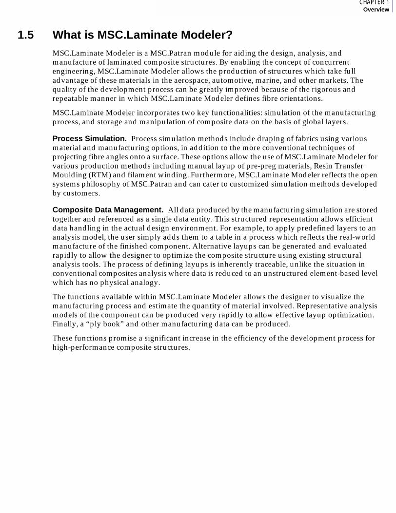
Definition of Developable SurfacesAn important subset of curved surfaces is developable surfaces. These surfaces can always be manufactured using sheet materials without the material needing to shear. At any point, there will be no curvature in one direction and maximum curvature in the orthogonal direction. Mathematically, this means that these surfaces are characterized by zero Gaussian curvature over their entire area. Cylinders are one example of developable surfaces found in many structures.

Note that all developable surfaces are ruled surfaces. However, not all ruled surfaces are developable. For example, a hyperbola of one sheet (such as a cooling tower shape) is not developable.

Although many CAD systems have provision for developing flat patterns from developable surfaces, the definition of material orientation is not trivial, particularly when the curvature is great.

The draping process for development is unique. That means that the cutout profile is always the same, and that definition of fibre orientation at any point uniquely describe the fibre orientations at all other points on the surface.

Ruled Surface

Simple NON-Developable Surface

Example of Waffle PlateOne example of a developable surface with complex fibre orientations is a waffle plate used as a core for sandwich structures. A typical geometry for a circular sandwich structure is shown in Figure 2-3. As the core is predominantly loaded in shear, it would be if the majority of fibres lay in the +/-45 directions along the webs. However, if these directions are ideal for one web, they will obviously not be the same for other webs.

Figure 2-3 Geometry of a Curved Waffle Plate

The MSC.Laminate Modeler can be used to quantify the effect of varying fibre orientation both qualitatively and quantitatively. For example, if a piece of woven fabric is draped from the middle rib so that the average angle is +/-45 along the webs of the central rib, we see that the angle on the webs near the edge of the plate are more like 0/90. This latter direction will obviously result in poor shear stiffness and strength in this direction.

Having understood this limitation, the designer can then make an informed decision whether to specify a quai-isotropic layup for the whole of the waffle plate, or to make the waffle plate out of several different plies oriented in different directions. Both alternatives can be modeled and analyzed rapidly using the MSC.Laminate Modeler, and an informed choice made on the basis of analysis results.

1CHAPTER 2Tutorial

Figure 2-4 Variation of Fibre Angles over Waffle Plate

Benefits of MSC.Laminate Modeler1. Visual feedback of fibre orientation.

2. Accurate orientation data for analysis model.

3. Exact flat-pattern generation.

2.5 Draping Simulation (Non-Developable Surfaces)

Definition of Non-Developable SurfacesNon-developable surfaces are those which cannot be formed from sheet material without the material shearing in its plane. Surfaces of this type have curvatures in two different directions (they are therefore often called doubly-curved surfaces). Although these surfaces are usually more difficult to manufacture than flat or developable surfaces, their form gives them great stiffness and strength.

Because composite materials can often shear during the manufacturing process, they are more suitable for manufacturing these shapes than conventional materials like aluminium. This magnifies the advantage of laminated composite materials for many classes of structure.

Gaussian Curvature. The extent of double curvature at any point is reflected in a value called the Gaussian curvature. This is the product of the curvatures in the principal directions at any point on a surface. The Gaussian curvature reveals many of the characteristics of a surface. Positive Gaussian curvature means that the surface is locally dome-shaped, with the curvatures in the same direction with respect to the surface normal. In contrast, negative Gaussian curvature implies saddle-shaped topology, with curvatures in opposite directions. Finally, zero Gaussian curvature is characteristic of a developable area.

Note that surfaces often have varying Gaussian curvature over their extent. As an example, a torus (donut) is saddle-shaped on the inside (negative Gaussian curvature) but dome-shaped on the outside (positive Gaussian curvature).

Gaussian curvature can be given a physical significance by drawing geodesic lines on a surface. (Geodesic lines are straight in the plane of the surface at any point; meridians are geodesic, but lines of latitude are constantly turning in one direction with respect to the surface.) A pair of lines which are initially parallel will tend to converge on surfaces of positive Gaussian curvature, but will diverge on a surface of negative Gaussian curvature. In contrast, the lines will remain parallel on the surface until they reach an edge if the surface is developable.

Another interpretation of Gaussian curvature is the extent of misfit in the surface. Consider a circular disk made up of several flat segments. This necessarily has zero Gaussian curvature even if it is bent along the joints between segments. However, if one of the segments is removed and the neighboring segments joined, the disk will adopt a dome-like shape which is indicative of positive Gaussian curvature. In contrast, adding a segment will result in the disk forming a saddle-like shape with negative Gaussian curvature.

Drape Simulation for Non-Developable Surfaces. Draping of non-developable surfaces is an extremely difficult task. Essentially, this process involves extremely large geometric and, perhaps, material nonlinearities. A direct consequence of this is that there is no unique solution for the draping process. The draped shape is highly dependent on the point at which the draping starts, the directions in which the draping proceeds and the properties of the material itself. In addition, if there is interaction between different layers, friction between them would have a significant effect. A detailed analysis of the draping process for arbitrary geometries is therefore a considerable analysis task in itself.

This difficulty in analysis reflects a real-world difficulty in manufacturing complex composite components consistently. Engineering drawings of composite components typically specify fibre angles within a tolerance of 3 degrees. In practice, if there is significant curvature in a surface, the manufacturing tolerance could easily reach 15 degrees or more.

2CHAPTER 2Tutorial

These problems can be mitigated to a large extent by limiting the degree of shear developed within reinforcing layers during the manufacturing process. The degree of shear is primarily dependent on the Gaussian curvature and the area of a layer. Therefore, a design incorporating two layers of excessive shear can be replaced by three smaller layers with less shear and greater quality. The MSC.Laminate Modeler employs a rapid draping module which allows the designer to investigate the likely degree of shear, and make rational engineering decisions on the basis of manufacturing simulations.

Whatever simulation process is used, two different levels of draping should be considered. Local Draping reflects the behavior of an infinitesimal material element applied to a point on a surface having general curvature. This is a material characteristic and is determined from tests on materials. In contrast, Global Draping considers how the many material elements are placed on a surface, and is dependent on the manufacturing process used.

Local Draping Models. Local draping is concerned with fitting a small section of material to a generally-curved surface. If the surface has nonzero Gaussian curvature, the material element must shear in its plane to conform to the surface. This deformation is highly dependent on the microstructure of the material. As a result, local shearing behavior can be regarded as a layer material property.

Figure 2-5 Scissor Draping Mechanism

Figure 2-6 Slide Draping Mechanism

MSC.Laminate Modeler currently supports two local draping algorithms: scissor and slide draping. For scissor draping (Figure 2-5), an element of material which is originally square shears in a trellis-like mode about its vertices to form a rhombus. In particular, the sides of the material element remain of constant length. This type of deformation behavior is characteristic of woven fabrics which are widely used to manufacture highly-curved composite components.

ashearedα

a

asheared

αa

For slide draping (Figure 2-6), two opposite sides of a square material element can slide parallel to each other while their separation remains constant. This is intended to model the application of parallel strips of material to a surface. It can also model, very simply, the relative sliding of adjacent tows making up a strip of unidirectional material.

When draping a given surface using the two different local draping algorithms, the shear in the layer builds up far more rapidly for the slide draping mechanism than for the scissor draping mechanism. This observation is compatible with actual manufacturing experience that woven fabrics are more suitable for draping curved surfaces than unidirectional pre-pregs.

For small deformations, the predictions of the different algorithms are practically identical. Therefore, it is suggested that the scissor draping algorithm be used in the first instance.

Global Draping Models. Global draping is concerned with placing a real sheet of material onto a surface of general curvature. This is not a trivial task as there are infinite ways of doing this if the surface has nonzero Gaussian curvature at any point. Therefore, it is important to define procedures for the global draping simulation which are reproducible and reflect what can be manufactured in a production situation. As a result, global draping behavior can be regarded as a manufacturing, rather than material, property.

The MSC.Laminate Modeler currently supports three different global draping algorithms: Geodesic, Planar and Energy. For the Geodesic global draping option, principal axes are drawn away from the starting point along geodesic paths on the surface (i.e., the lines are always straight with respect to the surface). Once these principal axes are defined, there is then a unique solution for draping the remainder of the surface. This may be considered the most “natural” method and appropriate for conventional laminating methods. However, for highly-curved surfaces, the paths of geodesic lines are highly dependent on initial conditions and so the drape simulation must be handled with care.

For the Planar global draping option, the principal axes may be defined by the intersection of warp (and weft for scissor draping) planes which pass through the viewing direction. This method is appropriate where the body has some symmetry, or where the layup is defined on a space-centered rather than a surface-centered basis.

Finally, the Energy global draping option is provided for draping highly-curved surfaces where the manufacturing tolerances are necessarily greater. Here, the draping proceeds outwards from the start point, while the direction of draping is controlled by minimizing the shear strain energy along each edge.

2CHAPTER 2Tutorial

Example of a Pressure Vessel. Many pressure vessels are made of composite materials, particularly via the filament winding process. However, it is often necessary to add woven reinforcements to the shell. In this case, it is vital to understand the mechanics of the draping process because the curvature of the surface varies so much. In particular, the body of a pressure vessel is developable and has zero gaussian curvature. In contrast, the ends have constant positive Gaussian curvature.

If draping begins at the pole of the vessel (Figure 2-7), the shear in the material increases rapidly away from the start point due to the severe curvature. The amount of shearing is indicated by the color of the draping pattern lines. Note that the degree of shear is zero along the principal axes, which are defined by geodesic lines.

The draping algorithm stops where the shear reaches the cutoff value for the material, or the override value defined in the Additional Controls form. This gives an indication of where the material would fold when being formed.

Figure 2-7 Fibre Directions for Draping Starting at the Pole of the Vessel

To cover the same area, it is also possible to begin draping on the cylindrical part of the surface (Figure 2-8). Because this region is developable, there is no shear deformation until the end cap is reached. This means that the average degree of shear on the surface is much lower, which should lead to better quality and better mechanical performance.

Figure 2-8 Fiber Directions for Draping Starting on the Cylindrical Part of the Vessel

Benefits of MSC.Laminate Modeler1. Visual feedback of fibre orientation.

2. Visual feedback of material shear.

3. Orientation data for analysis model.

4. Flat pattern generation.

2CHAPTER 2Tutorial

2.6 Building Models using Global Layers

Global Layer Description of LayupThe model is built up from predefined layers using a spreadsheet. This mirrors the use of layup tables in the final drawings of a component. The models are easily modified by defining, adding and deleting new layers to or from the layup.

Figure 2-9 Spreadsheet For Defining the Layup Using Predefined Layers

Example of a Top Hat SectionA typical top-hat section subjected to pressure and bending load will be used to illustrate the building of models using global layers. The model itself consists of a total of 52 global layers arranged in 4 different laminates. To model this structure properly, using conventional methods, would require the definition of 11 different property regions containing between 16 and 48 layers each. This would be tedious to define, and almost impossible to modify if the user wished to conduct a rapid sensitivity analysis.

Figure 2-10 Geometry of the Top Hat Section

2CHAPTER 2Tutorial

Figure 2-11 Lamination Specification of the Top Hat Section

In contrast, the MSC.Laminate Modeler user simply needs to define four layers which cover the areas of each laminate. Then, multiples of these layers are added to the model, using the layup spreadsheet. Because the surface is developable, it is permissible to use the Angular Offset option to modify the orientation of the plies at 45, 90 and -45 to the original layers. All the generation of representative property regions would be handled completely automatically by the software.

2

1

3

4

Laminate 1 [0/90/45/-45]4

Laminate 2 [0/90/90/0]

Laminate 3 [15/45]6

Laminate 4 [0/90/45/-45]5

Figure 2-12 Visualization of Geometry Covered by Layer_3

The greatest benefit would, of course, accrue if the model needed to be changed after a preliminary analysis. For example, the user may wish to define localized reinforcement at the attachment end of the section. This could be completed in a matter of minutes by defining additional layers and adding them to the layup.

Benefits of MSC.Laminate Modeler1. Rapid layer-based generation and modification of model.

2CHAPTER 2Tutorial

2.7 Results Processing

Recovering Results by Global LayerConventional systems present stresses on the basis of a particular layer on individual elements. If any element is reversed, or there are ply drop-offs on the surface, the produced results cannot be interpreted meaningfully.

In contrast, the MSC.Laminate Modeler rearranges analysis results stored in the database so that they refer to global layers defined in the layup spreadsheet. This means that the results for a physically meaningful piece of fabric are presented together. This is a unique capability for the majority of codes that store composite data on the basis of laminate materials.

Example of a Top Hat SectionFringe plots for stresses along the fibres are presented for global layers 1, 17, 21 and 33 for the top-hat section model. Using conventional post-processors, this would give misleading results due to the variation of layup over the model. In contrast, all stresses presented here are continuous, indicating that the correct results have been grouped for each global layer.

Figure 2-13

Figure 2-14 Layer Results


3CHAPTER 2Tutorial


Benefits of MSC.Laminate Modeler1. Flexible layer-based results processing.

2.8 Structural Optimization

Introducing Iteration to the Development ProcessThe ability to modify a composite model rapidly and asses results on a realistic basis opens up many opportunities for the optimization of composite structures. This is essential to compete with highly-optimized structures made of conventional materials, and bring the cost of composite structures down to a competitive level.

Example of a Torque Tube with a CutoutA tube subject to torsional loading and having a large cutout is representative of a number of structures, including the chassis of a single-seater racing car. A layup was defined, using two global layers covering the entire surface, and the rim around the cutout respectively as shown in Figure 2-17 and Figure 2-18.

Figure 2-17 Analysis Model of Torsion Tube

3CHAPTER 2Tutorial

Figure 2-18 Stiffened Collar

Models were built with a uniform layup, and including layer_2 reinforcement around the cutout. Analyses were then conducted for both configurations. As shown in the deformation plot in Figure 2-19, the torsional load generates substantial out-of-plane deflections around the cutout. Therefore, it is to be expected that reinforcing the cutout edge will have a significant effect on the structural performance of the tube.

Figure 2-19 Deformed Shape of Analysis Model

The analysis results for both models are summarized in the table below.

This clearly shows that the addition of local reinforcing in highly-loaded areas can have an extremely significant effect on overall structural performance. By allowing the designer to quantify the effects of localized reinforcement, the MSC.Laminate Modeler will enable the development of more efficient structures.

Benefits of MSC.Laminate Modeler1. Rapid modify-analyze-interpret cycle allows optimization.

Property Uniform Layup Reinforced Layup DifferenceLayup layer_1 (0/45/-45/90)

layer_1 (90/-45/45/0)layer_2 (0/45/-45/90)layer_1 (0/45/-45/90)layer_1 (90/-45/45/0)layer_2 (90/-45/45/0)

layer_2 (0/45/-45/90)layer_2 (90/-45/45/0)

Mass 4.826 kg 5.035 kg 0.209 kg (+4.3%)Rotation 0.143 0.118 -0.025 (-18%)Max. Deflection 2.817 mm 1.800 mm -1.017 mm(-36%)Max. Tensile Fiber Stress

165 MPa 122 MPa 43 MPa (-26%)

Max. Compressive Fiber Stress

186 MPa 121 MPa 65 MPa (-35%)

3CHAPTER 2Tutorial

2.9 Glossary(ISO 10303 equivalent terms in parentheses)

layer (Ply)

An area on a surface having consistent material properties, fiber orientation and thickness. A layer is analogous to one or more pieces of fabric which are applied to a surface adjacent to each other and in a similar way.

layup sequence (Layup_ply_table)

An assembly table which provides an ordered list of layers.

layup (Ply_laminate)

A collection of one or more layers which mate with one another.


CHAPTER

3 Using MSC.Laminate Modeler

■ Procedure

■ Element Library

■ Initialization

■ Creating Materials

■ Creating Plies

■ Creating a Layup and an Analysis Model

■ Creating Solid Elements and an Analysis Model

■ Creating Laminate Materials

■ Creating Sorted Results

■ Creating Failure Results

■ Creating Design and Manufacturing Data

■ Importing Plies and Models

■ Importing and Exporting Laminate Materials

■ Setting Options

■ Session File Support

■ Public PCL Functions

■ Data Files

3.1 ProcedureThe MSC.Laminate Modeler is a specialized tool for the creation and visualization of a ply-based laminated composite model. An analysis model consisting of appropriate laminate materials and element properties can be generated automatically for a number of different analysis codes. Following analysis, specific composite results can be calculated to verify the performance of the model. The general process for generating a laminate composite model is as follows:

1. Create Homogeneous Materials (MSC.Patran)

Materials are typically orthotropic, and the user should specify failure coefficients when defining materials.

2. Create Mesh (MSC.Patran)

The surface on which the composite layup is to be built is defined by the shell elements of the finite element mesh in the MSC.Patran database. The user should generate a mesh of sufficient resolution for both drape simulation and analysis purposes. It is a requirement that the meshing is completed before starting a session. Use the tools in the Finite Element application to verify the element normals and the free edges of the model before creating a new Layup file.

3. Create Ply Materials (MSC.Laminate Modeler)

These materials are analogous to raw ply materials and include a reference to a homogeneous material for specifying mechanical properties, as well as manufacturing related information like thickness.

4. Create Plies (MSC.Laminate Modeler)

Create plies in a manner which reflects the manufacturing process.

5. Create a LM_Layup and an Analysis Model (MSC.Laminate Modeler)

A layup, or sequence of plies, is defined, allowing the creation of corresponding laminate materials and element properties required to define an analysis mode..

6. Analyze (MSC.Patran and analysis code)

The analysis is submitted in the usual way. The user may have to explicitly request layered composites results from the analysis code.

7. Create Results (MSC.Laminate Modeler)

The user may sort results on the basis of physical plies or define new ones based on a failure analysis.

These operations are summarized schematically overleaf.

3CHAPTER 3Using MSC.Laminate Modeler

Overview

Figure 3-1 Overview of MSC.Laminate Modeler Process

Build MSC.Patran model. Generate MSC.Patran materials and required boundary conditions.

(NOTE: Finite Element model must be complete with model equivalenced.)

Existing Model having a MSC.Laminate Modeler Layup

file

New Model

Select MSC.Laminate Modeler from the Tools menu.

Choose a name for the Layup file.

(NOTE: A Layup file containing topology data is generated and opened.)

Select MSC.Laminate Modeler from the Tools menu.

Choose the previously created Layup file. An error will be indicated if the meshes in MSC.Patran and the Layup file are incompatible.

Generate LM_Materials as required.

Generate LM_Plies as required.

Generate LM_Layup as required.

Create analysis model and run analysis.

Review results and make modifications to the composite Layup. This can involve adding or modifying materials and/or LM_Plies. The Layup sequence may also be changed.

These actions can be mixed in order. For example, it is not necessary to generate all LM_Materials before starting to define the LM_Plies.

Sort results based on global plies and calculate failure criteria.

Open MSC.Patran database

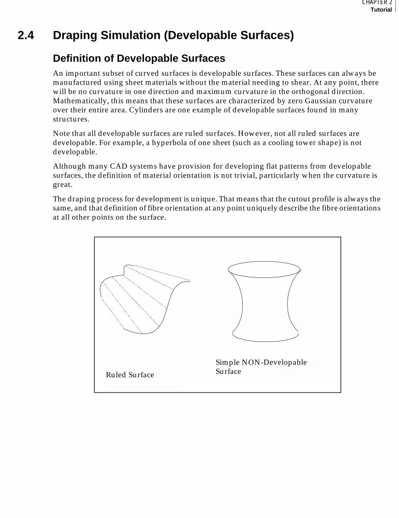
3.2 Element LibraryStandard shell elements define the surfaces used in the MSC.Laminate Modeler module. The standard MSC.Patran geometry and mesh generation commands can be used to create a valid model.

The elements in the MSC.Patran database are used to define the draping surface in addition to acting as analysis elements

Supported Element Topologies

Figure 3-2 Element Types

After the laminate descriptions have been generated they are applied to the Finite Element model in a controlled manner. The user is allowed to select the type of element for the currently selected analysis preference.

Tri/3 Tri/6 Quad/4 Quad/8


Supported Element Types1. Property selection and generation has been significantly enhanced from previous

versions. MSC.Laminate Modeler is no longer restricted to generating the data for MSC’s own preferences. Any suitably customized database will allow the generation of the required laminate materials and properties.

2. Selection of the thermal composite elements is now possible because of the redesign.

3. SAMCEF is supported by writing an external file for inclusion into the BACON BANQUE file.

Supported Element Property WordsThe routine for creating properties extracts the data from the database and compares it against values that are consistently used for the type of data required by MSC.Laminate Modeler.

The PROP_IDS that are recognized are:

If the applicable data type for the prop_ids described is not available, then the MSC.Laminate Modeler cannot generate the required property cards.

PROP IDS DESCRIPTION DATA TYPE

ID_PROP_MATERIAL_NAME(13) Laminated material name generated by MSC.Laminate Modeler.

MATERIAL_ID(5)

ID_PROP_ORIENTATION_ANG(20) This will be set to 0.0. The Laminate materials are built to reflect the different relative angles.

REAL_SCALAR(1)

ID_PROP_ORIENTATION_SYS(21) This prop_id is used to allow the creation of additional reference coordinate frames. Users are prompted whether or not they wish to create the frames.

COORD_ID(9)

ID_PROP_ORIENTATION_AXIS(1079) The property call is made reflecting the occurrence of this prop_id.

INTEGER_SCALAR(3)

3.3 InitializationThe initialization form controls the opening of the current MSC.Laminate Modeler database (Layup) file and the resultant display of the main Action Object Method control forms. To display the initialization form, select MSC.Laminate Modeler from the Tools menu.

Laminate Modeler

General Information...

Open Layup File...

Save a Copy...

Close

New Layup File...

Cancel

Save

Displays a form containing version information and the name of the current Layup file.

Allows the user to specify the name of a new Layup file. This file, containing only the topology of the shell elements in the open database, is then generated. Then the session begins and the main control forms are displayed.

Allows the selection of an existing Layup file. If the file exists, the MSC.Laminate Modeler session begins and the main control forms are displayed.

Copies the current Layup file to the name selected by the user. This does not alter the name of the current Layup file.

Closes the current Layup file and allows the user to open a new one.

Closes the current Layup file and hides the initialization form.

Saves the current Layup file.


3.4 Creating MaterialsWhen using MSC.Laminate Modeler there are three levels of material generation.

1. MSC.Patran homogeneous materials should be generated using standard MSC.Patran functionality. These contain mechanical, thermal or physical data which can be manually input or imported Using MSC.Patran Materials (p. 8) in the MSC.Patran Materials User’s Guide.

2. MSC.Laminate Modeler ply materials. These ply materials have thickness and manufacturing data in addition to a reference to an appropriate material in the MSC.Patran database. These ply materials are used to create plies in the MSC.Laminate Modeler module.

3. MSC.Patran laminate materials which are built up from MSC.Patran homogeneous materials by the MSC.Laminate Modeler software on the basis of the user-specified layup sequence, offsets and tolerances.

MSC.Patran Homogeneous Material Definition. The main description of the materials is done using the standard MSC.Patran methods of definition. The Materials form can be used to generate the required materials. Methods available include user input, external definition and MSC.Patran Materials.

MSC.Laminate Modeler Ply Material Definition. The homogeneous materials created, within the standard MSC.Patran form, are referenced within the MSC.Laminate Modeler Create LM_Material Add form to generate ply materials with extended property sets which include thickness and manufacturing data, such as the maximum strain allowable during draping.

Material Application Types. Ply materials are categorized by the way in which they are applied to a selected surface. They reference particular types of MSC.Patran homogeneous materials.

• Painted

Isotropic materials are supported for Painting.

• Projected

2D/3D orthotropic and anisotropic materials are supported for Projecting.

• Scissor Draped

2D/3D orthotropic and anisotropic materials are supported for Scissor Draping.

• Slide Draped

2D/3D orthotropic and anisotropic materials are supported for Slide Draping.

Additional Ply Material Parameters

• Thickness

• The thickness of a single ply of the material before it is sheared.

• Maximum Strain

The allowable strain value before the material “locks” (i.e., the material can no longer conform to the surface by shearing). This is measured in degrees.

• Initial Warp/Weft Angle

This value describes the original undeformed angle between warp and weft yarns in a fabric. This value can be overridden on the Create LM_Ply Add, Additional Parameters form. This allows deformation of the fabric before it is placed on the model, which may achieve better draping. This angle is measured in degrees.

Paint Project Scissor Slide

Thickness Yes Yes Yes Yes

Maximum Strain No No Yes Yes

Initial Warp/Weft Angle

No No Yes No


Create LM_Material Add FormThis form allows the user to generate MSC.Laminate Modeler ply materials which reference MSC.Patran homogenous materials and contain additional thickness and manufacturing data.

Laminate Modeler

Action: Create

Object: LM_Material

Method: Add

Type Drape (Scissor)

Existing LM_Materials

SC_Mat_1

LM_Material Name

SC_Mat_2

Analysis Material

fabric_t300_f934ud_t300_n5208

Refresh Material

Additional Properties

Thickness

0.1

Maximum Strain (degrees)

60.0

Warp/Weft Angle (degrees)

90.0

-Apply- Close

Application type. Options include: Drape (Scissor), Drape (Slide), Projected, Painted.

Unique name used to reference the LM_Material. The default name is of the form:

Mat_1After a new material is created, the numerical suffix (if any) of the name is identified and incremented by one, e.g. Mat_1 to Mat_2.

MSC.Patran homogenous materials generated using standard MSC.Patran functionality and which are appropriate for the relevant type.

If only one definition exists then it is selected automatically.

Additional properties required to define a LM_Material. These properties depend on the application type chosen.

Existing LM_Materials of the selected type.

Refreshes Analysis Material listbox. This is required if an analysis material is added while the Create LM_Material Add form is displayed.

Modify LM_Material Form

Laminate Modeler

Action: Modify

Object: LM_Material



SC_Mat_1

New LM_Material Name

SC_Mat_2

Analysis Material

fabric_t300_f934ud_t300_n5208

Refresh Material

Additional Properties

Thickness

0.1


60.0


90.0

-Apply- Close

Select the existing LM_Material to be modified.

Input the new material data as required.


Show LM_Material Form

Laminate Modeler

Action: Show

Object: LM_Material

Method: Form



SC_Mat_1

LM_Material Data

Analysis Material

ud_t300_n5208

Thickness

0.125


60.000004


90.

Close

Select the LM_Material to show.

Delete LM_Material Select Form

Laminate Modeler

Action: Delete

Object: LM_Material

Method: Select


PN_Mat_1PR_Mat_1SC_Mat_1SL_Mat_1

Select None

Select All

-Apply- Close

Select one or more LM_Material/s to be deleted.

If the LM_Material to be deleted is already included in an LM_Ply, it cannot be deleted and the user is warned. To remove such a material, first delete all LM_Plies which reference that LM_Material.


3.5 Creating Plies

What is a Ply? A ply is an area of LM_Material which is stored and manipulated as a single entity. A ply represents a piece of reinforcing fabric which is cut from sheet stock and placed on a mould during the manufacturing process. A ply is fully characterized by the LM_Material it is made of, the area it covers, and the way in which it is applied to the surface. The latter is particularly important for non-developable surfaces where there are many different ways of placing the fabric on a surface.

Figure 3-3 LM_Ply Description

Why use Plies? Plies allow easy manipulation of complex data when you assemble and/or modify the layers to form the complete layup. The physical representation of a ply is a piece of fabric.

Model Surface

First LM_Ply

Second LM_Ply

Create LM_Ply Add Form (Draping)

Laminate Modeler

Action: Create

Object: LM_Ply

Method: Add


Existing LM_Plys

SC_Ply_1SC_Ply_2SC_Ply_3

LM_Ply Name

SC_Ply_6

Select LM_Material

SC_Mat_1

Select Area

Element 1,2,5,6,9,10,13

Start Point

[24.999996 49.999996 0.]

Application Direction

<0. 0. -1.>

Reference Direction

<1. 0. 0.>

Reference Angle

45.

Additional Controls...

-Apply- Close

Application type. Options include: Drape (Scissor), Drape (Slide), Projected, Painted.

Unique name used to reference the ply.

The default name is of the form:

Ply_1After a new ply is created, the numerical suffix (if any) of the name is identified and incremented by one, e.g. Ply_1 to Ply_2

Existing LM_Materials of the selected type.

If only one material exists, then it is automatically selected.

Starting point of the application method.

Reference direction for the application method.

Reference angle between the reference direction and the initial warp orientation at the starting point.

Elements or Surfaces defining the extent of a ply.

Additional parameters required by the application method.

Note: When a ply is created, a group of the same name and containing the Area Definition entities is created.

Existing LM_Plies of the selected type.


Reference Angle

Reference Direction

Start Point

Reference direction for the application method.


Input Data Definitions

Start Point. This defines the starting point of the drape simulation process. It is analogous to the point at which a ply is first attached to a mould surface during manufacture. As the distortion usually increases away from the starting point, it is best to begin draping near the center of a region to minimize shear distortion. If the start point coordinates do not lie on the selected surface, the coordinates are projected onto the surface along the application direction vector. The start point must lie on the selected area.

Application Direction. The application direction defines the side of the surface area on which a ply is subsequently added when the final layup is defined. The “Top” of the surface covered by the ply is defined as the side on which the ply is originally applied when created. When defining a layup, the ply can be added to the “Top” or “Bottom” side of the mesh. It follows that the “Top” side is the same side as the application direction used to define the ply, whereas the “Bottom” side is the side opposite the application direction.

The concept of side is very important as composite structures are often built using molds or forms, limiting the side of application to a single direction. The plies of reinforcing fabric can be added to either the outside of a male mould or the inside of a female mould. When defining plies and a layup, it is useful to consider the manufacturing process.

The application direction is also used to project the start point and reference direction onto the surface.

Reference Direction. The reference direction is used to specify the initial direction of the fabric. The input vector is projected onto the surface along the application direction to define the principal warp axis of the material at the start point. Note that the direction of the material will usually change away from the starting point if the surface is curved.

Reference Angle. The principal warp axis of the material on the surface can be rotated from the reference direction by inputting a non-zero reference angle. This rotation is counterclockwise when viewed along the application direction.

For the same element, it is possible for different plies to have a different definition of the top side of the element depending on the application direction.


Top

Top


Figure 3-4 Effect of Application Direction on Warp Orientation

Note that the application direction is used to project the start point and reference direction vector onto the selected surface. This means that the same start point and reference direction vector results in different values when projected onto the surface along different application directions, as shown in Figure 3-4. It follows that the start point and reference direction should be defined as close to the surface as practical, while the application direction should be defined as perpendicular to the surface as possible.

Figure 3-5 Projection of Reference Direction

Viewpoint 1

Viewpoint 2

(a) (b)Reference Direction

Side Definition


Example of Starting Definitions

This example shows the view as it would appear in the viewport in addition to the input that would appear on the Create LM_Ply Add form.

Axis Type. The principal warp and weft axes are the paths the warp and weft fibers follow along the surface away from the start point. By defining the paths of the principal axes, it is possible to constrain the ply uniquely in the region bounded by the principal axes.

Application DirectionStart Point

Reference Direction

Start Point

[24.999996 49.999996 0.]


<0.1 -1.0 0.>

Reference Direction

<1. 0. 0.>

Reference Angle

0.

The principal axes can be defined in different ways:

• None

No principal axes are defined, draping proceeds using the extension method only.

• Geodesic

The principal axes are defined by geodesic lines from the start point.

• Planar

The principal axes are defined by the intersection of planes defined by the start point, application direction and reference direction rotated about the application direction through the reference angle.

Extension Type. The extension type controls the draping process if no axis type is defined, or the draping extends beyond the region uniquely defined by the principal axes. In this case, the material cells on each edge are kinematically unconstrained, and so some extension type must be specified to control the extension of the fabric.

The extension mechanism can be defined in different ways:

• Geodesic

The fiber closest to the principal axis is identified and extended along the surface along a geodesic path. The adjacent fabric cells are then uniquely constrained.

Note that the geodesic extension method yields an identical result to that produced using geodesic principal axes, followed by geodesic extension where necessary.

• Energy

The mechanism defined by the free edge cells is rotated in such a way as to minimize the shear strain energy in that free edge, using the assumption that the shear load-deflection behavior is linear (this could be extended for nonlinear response).

• Maximum

The mechanism defined by the free edge cells is rotated in such a way as to minimize the maximum shear strain in that free edge.

Start point

Principal warp axis

Principal weft axis

Boundary of uniquely constrainedregion

Boundary of region uniquelyconstrained by principal axes.

Free edge extending in accordancewith the extension type.


Additional Controls Form - Geometry

Additional Controls

Control Parameters

Geometry

Material

Boundaries

Order of Draping

Axis Type

None

Geodesic

Planar

Manual

Extension Type

Geodesic

Energy

Maximum

Step Length

Implicit Explicit

Input

1.0

OK

Sets the step length for the application simulation.

Implicit: Input value multiplies default step length

Explicit:Input value used for step length

Sets the axis type for the draping simulation.

None:There are no principal axes, and draping proceeds by extension only.

Geodesic:Principal axes are geodesic lines from the start point.

Planar:Principal axes are intersection of principal planes with the surface.

Manual:Define principal axes by selecting element edges.

Sets the extension type for the draping simulation.

Geodesic:The first extension yarn lies in a geodesic direction nearest the principal axis.

Energy:Draping proceeds from start point minimizing shear strain deformation energy.

Maximum:Draping proceeds from start point minimizing the maximum shear.

Additional Controls Form - Material

Additional Controls

Control Parameters

Geometry

Material

Boundaries

Order of Draping


Use Material Definition

Input

60.0

Warp/Weft Angle (Degrees)

Use Material Definition

Input

90.0

OK

Allows the user to override the maximum strain value for the layer material, which is first defined in the Create -LM_Material Add form.

The draping simulation stops if the maximum strain is exceeded. Elements on the undraped region are assigned extrapolated fiber orientations which should be checked before use.

Allows the user to override the warp / weft angle for the ply material, which is first defined in the Create LM_Material Add form.


Additional Controls Form - Boundaries

Additional Controls

Control Parameters

Geometry

Material

Boundaries

Order of Draping

Define Splits

Geometry Filter

Geometry FEM

Select Members

Elm 11.1.4

Add Remove

Split Definition

Element 7:9:2.1.1 6.1.3 7.1.4

Preview Split

Limit Fabric Size

Minimum Warp

Maximum Warp

Minimum Weft

Maximum Weft

OK

Select edges of elements to define an “interior edge” for the simulations.

Used when covering shapes like cylinders and cones. Also of use for introducing a “dart.”

Internal Boundary created to allow stopping of drape simulation

Figure 3-6 Split Example

Note: Avoid starting to drape near split definitions to prevent ambiguous draping results.

Simulate draping of material strips by limiting the fabric size as appropriate.

Flat and draped patterns are most clearly defined if the limit dimension is a multiple of the steplength.

warp

weft

Additional Controls Form - Order of Draping

Additional Controls

Control Parameters

Geometry

Material

Boundaries

Order of Draping

Order of Draping

Select Area

OK

1 Surface 1

2 Surface 6 7

3 Surface 9

Area

4 Surface 4

5 Surface 3

Surface 11:13Select a row numbered two or more and then select the required area using the standard selection utilities.

Note that the first row contains the area definition from the main Create LM_Ply form.

Note: This capability is particularly useful when draping over a series of conical sections. First drape the most critical section, ensuring minimal shear. Thereafter, drape peripheral areas.

First drape,minimumshear

Second drape

Third drape


Create LM_Ply Add Form (Projection)

Laminate Modeler

Action: Create

Object: LM_Ply

Method: Add

Type Projection

Existing LM_Plys

PR_Ply_1PR_Ply_2PR_Ply_3

LM_Ply Name

PR_Ply_6

Select LM_Material

mat.06mat.07

Select Area

Surface 1 2

Start Point

Node 18


<0. 0. -1.>

Projection Vector

Coord 0.2

Rotation about Normal

0.0

Method: Projected

-Apply- Close

This data is identical to that required for Draped plies.

Select the projection method, rotation angle and reference direction (where applicable).

Modify LM_Ply Form

Laminate Modeler

Action: Modify

Object: LM_Ply


Existing LM_Plys

Ply_1Ply_2Ply_3

LM_Ply Name

Ply_1

Select LM_Material

Mat_1

Select Area

Element 1,2,5,6,9,10,13

Start Point

[24.999996 49.999996 0.]


<0. 0. -1.>

Reference Direction

<1. 0. 0.>

Reference Angle

45.

Additional Controls...

-Apply- Close

The input data is identical to that required for creating plies.

Select the existing LM_Ply to be modified. This will fill the relevant databoxes with data required to rebuild the ply.


Show LM_Ply Graphics Form

Laminate Modeler

Action: Show

Object: LM_Ply

Method: Graphics


Existing LM_Plys

SC_Ply_1SC_Ply_2SC_Ply_3

LM_Ply Data

Start Point

<25. 50. 0.>


<0. 0. -1.>

Selected Area

Element 1 2 5 6 9 10 13

Reset Graphics

-Apply- Close

Select an existing LM_Ply to show. The start point, application direction and selected elements are placed in the appropriate databoxes.

On pressing Apply, the extent of the LM_Ply and the fiber angles are plotted in the viewport.

Delete LM_Ply Select Form

Laminate Modeler

Action: Delete

Object: LM_Material

Method: Select


PN_Mat_1PR_Mat_1SC_Mat_1SL_Mat_1

Select None

Select All

-Apply- Close

Select the LM_Ply to be deleted.

If the LM_Ply to be deleted is already included in an LM_Layup, it cannot be deleted and the user is warned. To remove such a LM_Ply, modify the LM_Layup so that it does not include the LM_Ply. The selected LM_Ply can then be deleted.

Note: When an LM_Ply is deleted, the group of the same name created at LM_Ply creation time will also be deleted.


3.6 Creating a Layup and an Analysis ModelThe individual LM_Plies are used to define the model LM_Layup using the Create LM_Layup Add form. When this form is selected, a spreadsheet for the Layup definition and forms for the relevant tolerances can be accessed. The forms are described on the following pages.

These forms are used to create and maintain the analysis layup. As well as providing tools to modify and redefine the layup, the forms will generate the correct laminate materials and apply the correct properties to the model. If all other operations are complete (i.e., Loads/BC addition), the model is ready for analysis after these forms have been applied.

Create LM_Layup Add Form

Laminate Modeler

Action: Create

Object: LM_Layup

Method: Add

LM_Layup Name

LM_Layup

Description

LM_Layup description

Layup Definition...

Offset Definition...

Generation Controls

Analysis Model

Select Element Type...Tolerance Definition...

Solid Elements

BACON file

-Apply- Close

Define the list of plies making up the LM_Layup.

Define the offsets.

Define the tolerances.

Create an analysis model using laminate materials.

Create a file containing solid elements.

Create a Samcef BACON file describing the analysis model.

LM_Layup name.

LM_Layup description.

Note that as only a single LM_Layup can exist per Layup file, the LM_Layup name and description are for information only.

Select the element type to be used.


Layup Definition Form

The spreadsheet is used to specify which of the previously defined LM_Plies are used in the generation of the model LM_Layup. The form allows the selection and ordering of the required LM_Plies. Manipulation of the LM_Plies within the spreadsheet is used to create different stacking sequences and layups.

Select the specific LM_Ply from the definitions in the Existing LM_Plies frame The method of application of that LM_Ply to the existing layup is controlled by the LM_Layup Controls. Continue by Adding, Inserting, and Deleting LM_Plies until the LM_Layup is finished.

LM_Plies can be added to the layup at any time to reinforce the model between analyses. The ability to redefine laminates rapidly is one of the key features of the MSC.Laminate Modeler.

The spreadsheet works in two distinct but connected modes. They are called “Expanded” and “Compressed.” In expanded mode, the multiplier column on the spreadsheet is always set equal to 1. This enables you to work at the level of single LM_Plies and the Delete and Replace commands will only act on the single LM_Ply selected. In compressed mode, the Delete and

Report: Send the current LM_layup definition to the report file. This will be replaced by the Create Ply Book command.

Clear All: Clear current definition from spreadsheet.

Expand: Toggle between “Expanded” and “Compressed” mode.

Utilities: Not currently activated.

Multiplier: Number of times that the specified add action is to take place.

Angle Offset: Modification parameter by varying the actual angles by a specified amount. Applicable for small angles only.

Allowable Actions:

Add: The selected LM_Ply in the listbox is added multiplier times.

Insert: the selected LM_Ply is placed in to the stack multiplier times.

Replace: The selected row on the spreadsheet is replaced by the listbox LM_Ply. The multiplier value on the spreadsheet is used to determine the number of LM_Plies to replace.

Show: The selected LM_Ply is displayed on-screen.

Delete: The spreadsheet selected LM_Ply is removed. The multiplier value is used to determine how many LM_Plies to remove.

Element Layup Report

LM_Layup definition

Stacking Sequence Convention:

Current LM_Ply: 0

OK

Total

Slide 1 Top1 SL_Ply_1

2 SL_Ply_2

3 SL_Ply_3

4 PN_Ply_1

1.1Steel

Steel

Alum

AlumPN_Mat1

SL_Mat3

SL_Mat2

SL_Mat1

0.3

0.1

0.1

90.

180.

180.

180. Painted

Slide

Slide

2

1

1

Top

Top

Top

Type Instance SideLM_Ply Thick.Anal. MatMaterial Ref Ang

LM_Layup definition (Compressed)

LM_Layup controls

Action: Add

Multiplier 1

Angle Offset0.0

LM_Layup DataNumber of LM_Plys: 20

Report Clear All

Utilities Expand

Existing LM_Plys

PN_Ply_1PN_Ply_2PN_Ply_3

Replace commands can be used to do multiple “single actions” at the same time. For example, if a row is specified as having a multiplier of 10, then a replace instruction will replace all 10 rows with the new LM_Ply. The same is true for delete.

You can switch between the two methods at any time and take advantage of the quicker set up time of the stack building, while still being able to modify the LM_Ply sequence at the single LM_Ply level if required.

Make current definition a total definition.

Make the current definition symmetrical by copying LM_Plies.

Make the current definition symmetrical about the bottom LM_Ply.

Split the current definition in half.

Split the current definition in half as if the current definition is symmetrical about a mid-LM_Ply.

Cut data from selected spreadsheet cells.

Copy data from selected spreadsheet cells

Paste data cut or copied from selected spreadsheet cells

Paste mirrored data cut or copied from selected spreadsheet cells

Undo the last command for the LM_Layup definition spreadsheet.

Figure 3-7 Icons on LM_Layup Create Spreadsheet


Offset Definition Form

Offset Value: The amount that the reference plane is offset from the shell surface towards the viewer (negative value is away from viewer).

Offset Flag: Position of layers relative to reference plane from view point.

Reference

Reference

Reference

VIEW DIRECTION

MIDDLE

TOP

BOTTOM

Shell Surface

Offset Value

Shell Surface

Offset Value

Shell Surface

Offset Value

Offset Controls

Select Mode

Ignore Offsets

Define Offsets

Values

Select Area

Definition Point

Definition Direction

Offset Value 0.0

Offset Flag Middle

Create Delete

OK

1

2

3

Area

4

5

Define Offsets

Surface 6:7

Surface 3

Surface 8

Surface 16

Surface 1

Important: Ignore Offsets is required for analysis preferences like ABAQUS and MSC.Patran Advanced FEA which do not allow any offset definition for composite shells. This is not the same as having an offset = 0.0. An offset with a specified value will cause an error as it is interpreted as a set value.

Select Element Type Form

Select Element Type

Composite Element Types

Analysis Code MSC.Nastran

Analysis Type Structural

Select Type

2D_Stan. Lam. Plate (CQUAD4/PCOMP)2D_Rev. Lam. Plate (CQUADR/PCOMP)

OK Cancel

This databox lists all element types in the current Analysis Preference which can accept the relevant materials.

Select the element type to be generated by Laminate Modeler.


Tolerance Definition Form

Tolerance Controls

Select Mode

Ignore Overrides

Override Regions

Global

Ang. Tol. (deg.) 5.0

Thck. Tol. (%) 5.0

Values

Select Area

Ang. Tol. (deg.) 5.0

Thck. Tol. (%) 5.0

Create Delete

OK

1

2

3

Area

4

5

Define Offsets

Surface 3

Surface 1:2

Surface 5

Surface 4

Surface 6

Critical area

Input global angular tolerance.

Input global thickness tolerance.

For each override tolerance area:

Select the appripriate row of the spreadsheet.

Define the appropriate data: Area, angular tolerance, and thickness tolrance.

Press Create to update the data in the spreadsheet (or Delete to delete the data)

Modify LM_Layup Add Form

As only a single layup is allowed in a single Layup file, the form for layup modification is identical to that for layup creation.

LAMINATE MODELER

Action: Modify

Object: LM_Layup

Method: Add

LM_Layup Name

LM_Layup

Description

LM_Layup description

Layup Definition...

Offset Definition...

Generation Controls

Analysis Model

Select Element Type...

Tolerance Definition...

Solid Elements

BACON file

-Apply- Close

Define the list of plies making up the LM_Layup.

Define the offsets.

Define the tolerances.

Create an analysis model using laminate materials.

Create a file containing solid elements.

Create a Samcef BACON file describing the analysis model.

LM_Layup name.

LM_Layup description.

Note that as only a single LM_Layup can exist per Layup file, the LM_Layup name and description are for information only.

Select the element type to be used.

Existing LM_Layup

LM_LayupExisting LM_Layup.


Show LM_Layup Exploded View Form

This capability allows the user to verify the definition and application direction of the plies defined in a layup.

Unselects all plies in listbox.

Selects all plies in listbox.

Shows LM_Layup name.

Select one or more plies in LM_Layup to show.

Clears all Show LM_Layup graphics from the viewport.

Sets distance between exploded plies.

LAMINATE MODELER

Action: Show

Object: LM_Layup

Method: Exploded View

LM_Layup Name

LM_Layup

Set Labels...Select LM_Plies

LM_Layup.1LM_Layup.2LM_Layup.3LM_Layup.4

Select None

Select All

Offset Dist. Multiplier

10.00.0

Display Options


LM_Ply Labels

Reset Graphics

-Apply- Close

Change LM_Ply labels in listbox and on screen.

Set Options for display in viewport.

Show LM_Layup Cross Section Form

This capability allows the user to define cross-section plots of the plies defined in a layup.

Set the thickness scale for LM_Plies in the viewport.

Define the Section Plane Normal by selecting the axis of a coordinate systeml.


Set the thickness shrinkage of the LM_Plies in the viewport.

Define the Offset from the origin of the selected coordinate system.

Action: Show

Object: LM_Layup

Method: Cross Section

Define Section Plane Normal

Coord 0.3

Offset Parameters

Offset

0.0

Thickness Scale

10.00.0

Thickness Shrinkage

1.000.00

Reset Graphics

-Apply- Close

LAMINATE MODELER


Show LM_Layup Element Form

This capability allows the user to verify the resulting layup on individual elements. Visualization capabilities are similar to those provided by the Show Laminate function.

Select an element to show.


Select if an informational spreadsheet is displayed.

Action: Show

Object: LM_Layup

Method: Element

Auto Execute

Select Element

Plot Markers

Element Normal

Orientation

Thickness

Thickness Scale

10.00.0

Thickness Shrinkage

1.000.00

Layup Report

Reset Graphics

-Apply- Close

LAMINATE MODELER

Select which graphics to display to the viewport.

Set the thickness of LM_Plies in the viewport.

Set the thickness shrinkage of the LM_Plies in the viewport.

Select if any graphics to display to the viewport.

Show LM_Layup Element Info Form

Element Layup Report

OK

Slide 1 Top1 SL_Ply_1

2 SL_Ply_2

3 SL_Ply_3

4 PN_Ply_1

1.1Steel

Steel

Alum

AlumPN_Mat1

SL_Mat3

SL_Mat2

SL_Mat1

0.3

0.1

0.1

90.

180.

180.

180. Painted

Slide

Slide

2

1

1

Top

Top

Top

Type Instance SideLM_Ply Thick.Anal. MatMaterial Ref Ang

This form displays all plies in the order in which they appear on the element. This is particularly useful for identifying problems relating to application directions when defining a Layup.


Transform LM_Layup Mirror Form

This capability allows the user to model a repeated unit of a symmetrical model, and mirror as appropriate to generate the full model. For example, only one half of a composite chassis may be modeled prior to mirroring the mesh and layup about the center plane.

Action: Transform

Object: LM_Layup

Method: Mirror

Mirror Elements

Numbering Option

Starting ID(s) 17

Define Mirror Plane Normal

Coord 0.3

Offset Parameters

Offset

0.0

Reverse Elements

Equivalence Elements

Equivalencing Tolerance

0.005

Mirror Plies

Prefix

M-

Add Plies to Layup

Reset Graphics

-Apply- Close

Select element numbering.

Define the Section Plane Normal by selecting the axis of a coordinate system.


Define the Offset from the origin of the selected coordinae system.

Equvalence elements.

Equvalencing Tolerance.

Mirror the LM_Plies.

LM_Ply prefix.

Add the new plies to the Layup.

Delete LM_Layup Select Form

This form allows the user to delete the single layup defined in the current Layup file.

LAMINATE MODELER

Action: Delete

Object: LM_Layup

Method: Select

Select None

Select All.

-Apply- Close

Existing LM_Layups

LM_LayupExisting LM_Layups.


3.7 Creating Solid Elements and an Analysis ModelThe MSC.Laminate Modeler defines a ply layup on a 2D shell mesh. The majority of analyses can be conducted using shell elements as through-thickness effects are relatively insignificant. However, if the laminate is thick, and especially if the surface is curved, it may be necessary to use solid elements to model structural behavior adequately.

For these situations, the MSC.Laminate Modeler includes the capability to extrude shell elements through a distance equal to the laminate thickness. Furthermore, laminate materials and element properties can be created automatically to allow accurate analysis. If the analysis code does not support laminated solid elements, the laminate materials are converted to equivalent anisotropic materials for subsequent analysis.

Create Solid Elements LM_Layup Form

This capability allows the user to generate solid elements and the associated materials and element properties needed for detailed analysis of thick laminates.

Select elements or All.

Select node and element numbering.

Create a Patran group.

Preview the action.

Reset the viewport graphics

Laminate Modeler

Action: Create

Object: Solid Elements

Method: LM_Layup

Select Area

Select: All

Select Elements

Numbering Option

Node

Starting ID(s) 26

Element

Starting ID(s) 17

Create Group

Group Name

LM_Solid_Elements

Preview...

Reset Graphics

-Apply- Close

Analysis Model



Create an analysis model by generating laminate materials and element properties as required by the analysis code.

The elementtype and tolerances must be set as required.


3.8 Creating Laminate MaterialsThe MSC.Laminate Modeler generates laminate materials and element properties when creating or modifying a layup, or when creating solid elements. Additional capabilities are provided for advanced users who need greater control over the creation of the analysis model. For example, when using MSC.Nastran, the user can align the laminate materials using several different methods such as using coordinate systems or specified vectors.

The procedure followed for generating an analysis model is as follows. The MSC.Laminate Modeler stores warp angle, weft angle and thickness data for every element making up a ply. When a layup is created, the total material definition on every element can be defined. By default, angle data is specified with respect to the first edge of every element.

The next step is to transform this angle data to the angle definition system required by the selected element type. For example, the projection of a vector onto each element may be used as the basis for defining laminate material orientations. This allows the program to calculate a corresponding laminate material on each element.

However, it is generally unwieldy to define a laminate material per element for large models which may contain over a hundred thousand elements. Hence, a sorting mechanism is invoked to identify a minimum number of materials within the user-defined tolerance.

The analysis model can become complicated due to the continuous variation of fiber direction over curved surfaces. Verification tools allow the user to show the layer thickness and orientations on any element in the model. This capability can be used even if conventional techniques have been used to define the composites model, or legacy analysis files have been imported into MSC.Patran.

Create Laminate LM_Layup Form

Laminate Modeler

Action: Create

Object: Laminate

Method: LM_Layup

Select Area

Select: All

Select Elements

Laminate Orientation

Vector

Primary Vector

Coord 0.1

Switch Angle

0.1

Secondary Vector

Coord 0.2


Laminate Options...

Preview...

-Apply- Close

Select the element type required for the analysis.

Select the element dimension and material type of the element properties to be created. The element types available are dependent on the capabilities of the current analysis code.

Select the elements for which laminates and properties are to be generated. Choosing ALL selects every shell element in the database.

Select the basis for the laminated orientation, which is dependent on the analysis code. For example, MSC.Nastran allows orientation definition by means of a coordinate system, vector ar angle with respect to the first edge of every element.

Set the tolerance definition for laminate generation.

Optionally, set the prefix and starting numbers for laminates and properties.

Preview the number of laminates and properties to be generated.


Dimension: 2D

Material: Laminate


Laminate Options Form

Preview Form

Laminate Names

Prefix new_lams.

First Laminate Id 1001

First Property Id 20001

OK

Define a prefix for the laminates and properties.

Define the first laminate ID, e.g.

new_lams.1001

Define the first laminate ID, e.g.

new_lams.20001

Preview

Number of Coordinates

0

Number of Laminates

8

Number of Properties

8

Cancel

Displays the number of coordinate systems, laminates and properties to be generated.

Show Laminate Form

Laminate Modeler

Action: Show

Object: Laminate

Select Area

Elm 16

Select Property Sets

LM_Layup_8

Select Laminates

LM_Layup_8

Select Property

Existing Properties

MaterialOrientationThickness

Type: Real Scalar

Display Method Model Plot

Select Layers

12

7Thickness Scale

10.00.1

Reset Graphics

Apply Close

Select elements defining display region.

The property sets referenced by the selected elements are displayed. Select one or more of the property sets.

The laminates referenced by the selected property sets are displayed. Select one or more of the laminates.

Select the laminate property to be displayed.

Select the display method.

Select the relevant display options, such as layers to be displayed and the thickness scale.


Delete Laminate Select Form

Laminate Modeler

Action: Delete

Object: Laminate

Method: Select

Existing Laminates

LM_Layup_1LM_Layup_2LM_Layup_3LM_Layup_4LM_Layup_5

Select None

Select All

-Apply- Close

Select one or more laminates to be deleted.

If the laminates are referenced by property sets, the user is asked whether the property sets should also be deleted.

Delete Property Set Select Form

Action: Delete

Object: Property Set

Method: Select

Existing Property Sets

LM_Layup_1LM_Layup_2LM_Layup_3LM_Layup_4LM_Layup_5

Select None

Select All

-Apply- Close

Select on or more property sets to be deleted.

Laminate Modeler


3.9 Creating Sorted ResultsMost analysis codes which generate results for laminated composite materials define the layer results as the stacking sequence number with respect to the element orientation system. If there are ply drop-offs or elements are reversed, the stacking sequence number bears no direct relationship to the physical plies.

To overcome this problem, two results sorting procedures are supported. If the analysis model has been generated using laminate modeler, the results can be sorted quite simply using data stored in the Layup file. Otherwise, results can be sorted on the basis of underlying material IDs, if the ID is only used once on every element over a selected area.

Create LM_Results LM_Ply Sort Form

LAMINATE MODELER

Action: Create

Object: LM_Results

Method: LM_Ply Sort

Select Result Cases

1-DEFAULT

Select Layered Result

3.1-Strain Tensor, 4.1-Curvature Tensor, 6.1-Stress Tensor,

-Apply- Close

See Session File Support (p. 104).

This form allows the user to sort results with respect to LM_Plies.

Existing results are rearranged to create new sets of layered results that reflect the actual LM_Plies used in the laid-up model.

The results themselves are not changed but simply placed into new groups.

The number of the global plies corresponds to the row of the LM_Ply in the LM_Layup definition spreadsheet.

Select result cases.

Select layered result.

Set Ply Labels Displays a form to modify the Ply labels.


Create LM_Results Material ID Sort Form

LAMINATE MODELER

Action: Create

Object: LM_Results

Method: Material ID Sort

Select Result Cases

1-Default



Select Area

Select Materials

mat.01mat.02mat.03mat.04mat.05

-Apply- Close



Select elements over which results will be sorted.

Select material ids according to which the results will be sorted.

Only materials occurring only once on every selected element will be displayed.

Elm 1:16

3.10 Creating Failure ResultsFailure indices according to various criteria can be calculated from layered results.

Note that these are based on calculated results and do not affect the analysis model itself. Therefore, they rely on the assumption of linearity and are only valid for first ply failure.


Create LM_Results Failure Calc Form

LAMINATE MODELER

Action: Create

Object: LM_Results

Method: Failure Calc

Select Result Cases

1-DEFAULT



Select Area

Elm 6:8 10:12 14:16

Criterion: Maximum

Material Allowables...

Create Results

Name TEST_1

Margin of Safety

Critical Component

Critical Ply

Ply-by-Ply Results

-Apply- Close



Select the area.

Select the failure criterion.

Input material allowables.

Define output requests.

Material Allowables Form

Material Allowables

Cell Value = 0.0

OK

mat8.1 2464015001500

200200200200

Yc Yt Xc Xt

-0.5505068

0115115115

F12 S31 S23 S12

Stress

mat8.2

The laminate materials referenced at least once over the selected area are placed in spreadsheet rows. If they have failure properties defined, these are placed in the appropriate columns of the spreadsheet.

The user can modify values to allow a “what-if” capability. Changed values can be saved to the database using the "Save to Db" button. Original values stored in the database can be restored to the spreadsheet using the "Get from Db" button.

If the out-of-plane shear allowables are zero, then the out-of-plane shear allowable is not calculated.

Save to Db Get from Db


3.11 Creating Design and Manufacturing DataIt is important to integrate the design, analysis and manufacture of laminated composites. In particular, it is important that the model analyzed is equivalent to the manufactured part. Therefore, a ply book containing design and manufacturing data can be produced at any time.

Create Ply Book Layup Form

LAMINATE MODELER

Action: Create

Object: Ply Book

Method: LM_Layup

LM_Layup Name

LM_Layup

Select LM_Plys

LM_Layup.1 (Paint,PN_Ply_1,TLM_Layup.2 (Paint,PN_Ply_2,TLM_Layup.3 (Paint,PN_Ply_3,TLM_Layup.4 (Paint,PN_Ply_4,TLM_Layup.5 (Paint,PN_Ply_5,T

LM_Layup.9 (Project,PR_Ply_4,Top)

LM_Layup.11 (Slide,SL_Ply_1,Top)

Select None

Select All

Layup Report

Ply Data

Export Options...

Display Options...

Image Creation

-Apply- Close

If active, a text report of the layup is generated. This can be imported into other applications such as spreadsheets.

If active, the selected plies are recreated on-screen in the layup order.

Optionally, a postscript file of the viewport can be generated to create a printed record of the ply.

Display options can be set to display the required ply information in the viewport.

Export options can be set to generate the required manufacturing data.

The layup report contains the same data as the spreadsheet used to create the layup. The user can diplay expanded or compressed, and select which data are written to the report file.

Shows LM_Layup name.

Select one or more plies in LM_Layup to include in the Ply Book.

Unselects all plies in listbox.

Selects all plies in listbox.

Set Labels... Change LM_Ply labels in listbox.

Expand Compress

IndexLM_Ply

TypeMultiplierSideAngle Offset

Reference AngleThicknessLM_Material

3.12 Importing Plies and ModelsUsually, a new Layup file is created once a mesh has been finalized in the MSC.Patran database. If the user subsequently changes the mesh, the elements in the database and those in the Layup file no longer correspond. This can lead to errors because the elements selected in the viewport may not have the same IDs as those used for internal operations. For this reason, a warning is issued if the database mesh does not correspond to the Layup file mesh when opening a new Layup file.

In addition, it may be desirable to import plies from another Layup file, which may have a different element definition. For example, a draping simulation tool embedded in a CAD package could generate a Layup file which has no knowledge of the analysis mesh.

The Import Ply capability has been developed to allow users to remesh as required and also import of data from other draping systems. In order to do this, it is necessary to generate a mapping between the current mesh and the imported mesh. This mapping is calculated by element matching or piercing.

The MSC.Laminate Modeler first tires to find a direct match between current and imported elements by identifying elements with the same nodal coordinates. Where such a match is identified, the layup on the imported element can be transferred directly to the current element as necessary. The matching process is relatively fast.

Where a current element has no direct match, mapping is determined through piercing. Here, a normal vector is calculated at the centroid of each current element and any intersections with imported elements are calculated. If there are multiple intersections, that closest to the centroid is chosen. The distance between the centroid and intersection point is calculated, as is the angle between the current normal and the normal of the intersected imported element. If both the calculated distance and angle are less than the distance and angular tolerances respectively, the layup on the intersected element is mapped onto the current element. This piercing process is relatively slow due to the multiple calculations required.

In addition to ply import, it is also possible to import a complete composites model definition stored in a Layup file. This will copy the mesh and materials from the Layup file into a MSC.Patran database so that further operations like ply creation can be conducted as normal. This feature means that composite models can be transferred and stored by means of the Layup file alone.

centroid of current element with normal

closest intersection point of normal with

current surface mesh imported surface mesh

imported elements


Import Plies File Form

Laminate Modeler

Action: Import

Object: Plies

Method: File

Select Directory...

Existing Plies

plate_matid

Select All

Select None

Angle Tolerance (deg)

25.0

Distance Tolerance (%)

5.0

-Apply- Close

Select the directory containing Layup files to be imported.

Select the Layup (ending .Layup) and directory (ending .fmd) files to be imported. The files are imported in the order shown in the listbox. Directory files are displayed in square brackets "[]". If selected, all files specified in the directory file are imported.

Set the angular and distance tolerance for defining adjacency of dissimilar elements.

Add the layup of the imported file to the layup defined in the current session.

Preview

Merge Nodes

Import Layup

Plot the imported plies in the viewpoint and ask user for confirmation before mapping to the current mesh.

Merge the nodes in the imported Layup files before calculating and plotting the boundaries of files in that directory.

[directory1]

Select all files.

Unselect all files.

Import Model File Form

Laminate Modeler

Action: Import

Object: Model

Method: File

Mesh

Node ID offset

25

Element ID offset

16

Create Group

Group Name

plate

Materials

-Apply- Close

Imports the mesh form the current Layup file into the MSC.Patran database.

Imports the analysis materials in the current Layup file into the MSC.Patran database.

The minimum required node and element ID offsets to prevent duplication (that is, the highest database ID less the lowest Layup file ID plus 1) are displayed.

Note that if the offsets are non-zero, the database mesh will not correspond with the Layup file mesh.

Optionally puts imported mesh in a group. The default name of the group is the name of the layup file.


3.13 Importing and Exporting Laminate MaterialsThe MSC.Laminate Modeler generates laminate materials based on a ply layup. However, under certain circumstances, it is desirable to export or import laminate materials to or from specialized tools used for laminate analysis. The MSC.Laminate Modeler includes and interface to the LAP laminate analysis program developed by Anaglyph Ltd. (www.anaglyph.co.uk).

During preliminary design, the user can define a baseline laminate material within LAP and save this data in a text file. This information can be imported into MSC.Patran and referenced by element properties in the normal way. This basic laminate can be optimized for loading and manufacturing criteria using the tools within the MSC.Laminate Modeler.

Following analysis, the user can export laminate material and load information to LAP in order to examine and report stresses.

Import Laminate LAP Form

Laminate Modeler

Action: Import

Object: Laminate

Method: LAP

Select Data File...

-Apply- Close

Select the LAP text file containing Material and Laminate Material information.


Export Laminate LAP Form

Laminate Modeler

Action: Export

Object: Laminate

Method: LAP

-Apply- Close

ElementSelect Laminate by:

Select Element

Elm 6

Select Laminates

Laminate_1Laminate_2 Laminate_3

Select Data File...

Export Forces

Delete New Coords

Select Loadcases

Loadcase_1Loadcase_2 Loadcase_3

Spawn LAP

Set the laminate selection mechanism.

If selection is by element, all laminate materials referenced by those elements appear in the Select Laminates listbox.

If selection is by list, all laminate materials in the database appear in the listbox.

Select the laminates to be exported.

Select the LAP text file to be created. The default name is “pat_to_lap.txt”.

Loads may be exported if the laminate on a single element is selected.

The user selects one or more loadcases. A coordinate system aligned with the laminate is created and analysis results extracted in this coordinates system.

The user can specify if the coordinates should be deleted after calculation.

LAP can be spawned automatically if running on Windows systems. The environment variable LAP_EXE_PATH must be set to the required LAP executable.

3.14 Setting OptionsOptions for the display of graphical information in a viewport, and the export of manufacturing data, must be set before creating plies and layups.

Set Export Options Form

Laminate Modeler

Action: Set

Object: Export

Method: Options

LM_Ply Files

Export Options...

LM_Layup Files

Mold Surface

IGES

-Apply- Close

Define the files to be exported when a ply is created or modified. These include the draped and flat patterns, in IGES or DXF format.

Define the files to be exported when a layup is created. This includes a faceted represenatation of the mould surface in IGES format.

Export Options

LM_Ply Files

Draped Pattern

IGES

DXF

Flat Pattern

IGES

DXF

Curve POLYLINE

Layer POLYLINE

OK Reset


Flat Pattern Example

Figure 3-8 Example Flat Pattern

The 2D flat pattern shape can be generated in different formats. The DXF format is typically used to drive nesting and cutting machines.

Note that the flat pattern shape does not indicate the edges of the fabric where the maximum strain value has been exceeded.

Set Display Options Form

Laminate Modeler

Action: Set

Object: Display

Method: Options

Additional Forms

Message File

LM_Ply Display Control

LM_Layup Display Control

LM_Ply Graphics

Display Options...

LM_Layup Graphics

Surface Offset

Scale

10.00.1

-Apply- CloseInput the scaling of the offset arrow drawing for outermost ply plotting.

Material: Plot/Erase the material from which the ply is made.

Application Direction: Plot/Erase an arrow showing the Application DIrection.

Reference Direction: Plot/Erase an arrow showing the Reference Direction.

Selected Area: Plot/Erase the boundary and outline of the selected area.

Maximum Strain: Plot/Erase the title showing minimum and maximum relative strain, absolute strain and thickness.

Angles: Plot/Erase arrows showing warp and weft directions on individual elements.

Draped Pattern: Plot/Erase the draped pattern.

Flat Pattern: Plot/Erase the flat pattern on a plane perpendicular to the application direction.

Offset: Distance from start point to flat pattern plane.

Display the message file, the LM_Ply Display Control form, or the LM_Layup Display Control form.

Display Options

LM_Ply Graphics

Material


Reference Direction

Selected Area

Maximum Strain

Angles

Draped Pattern

Flat Pattern

Offset

0.0

OK Reset


Additional Forms Controlling Ply and Layup Graphics

LM

LM

Hides form and erases graphics.

Directions: Plot/Erase arrows showing the Application and Reference DIrections.

Selected Area: Plot/Erase the boundary of the selected area.

Selected Area: Plot/Erase the outline of the selected area.

Draped Pattern: Plot/Erase the draped pattern.

Flat Pattern: Plot/Erase the flat pattern on a plane perpendicular to the application direction.

Maximum Strain: Plot/Erase the title showing minimum and maximum relative strain, absolute strain and thickness.

Angles: Plot/Erase arrows showing warp and weft directions on individual elements.

Material: Plot/Erase the material from which the ply is made.

Surface Angles: Plot/Erase arrows showing warp and weft directions on the top and bottom surfaces of individual elements.

Hides form and erases graphics.

Flat Pattern Display on Screen

Figure 3-9 Flat Pattern Displayed on Screen

The flat pattern shape is displayed on the screen perpendicular to the application direction arrow. The variation that occurred between the draped fabric on the model and the undeformed fabric shape can be seen.


Reference Direction


Figure 3-10 Flat Pattern Displayed for Surface with Split Definition

3.15 Session File SupportMSC.Laminate Modeler can be run from a session file if required. The session file should contain calls to the public PCL functions defined in the next section. These functions correspond to user interface forms in the usual way. If required, the contents of a session file can be modified manually before being replayed to change the layup.

Replaying a session file also allows the user to remesh surfaces if area selection is done by reference to geometrical entities, such as <Surface 4 8>. However, care must be taken with the selection of the start point and the reference direction to make sure that they correspond to the remeshed model.

Note that running a session file will be slightly different from undertaking an interactive run because the forms will not appear or be filled with the corresponding data.

It is also advisable to change the full path names for the files to just the file names. For example: “/usr/people/demo/test/testrun. Layup” becomes “testrun.Layup”.

Important: Session File edits.


3.16 Public PCL FunctionsThese functions correspond to user interface forms in the usual way. They can be used by running a session file, or calling them directly from other PCL functions. In either case, it is important that the PCL library <laminate_modeler.plb> is available to the session, and the executable <layup> is in the path.

Begins a MSC.Laminate Modeler session using a new Layup file with the name <filename>.

Begins a MSC.Laminate Modeler session by opening an existing Layup file with the name <filename>.

Saves a copy of the current Layup file with the name <filename>.

p3cm.new ( <filename> )

Input:STRING <filename> Name of the new Layup file.Output:INTEGER <Return Value> Status return value. The value will be 0 if the

routine is successful.

p3cm.open ( <filename> )

Input:STRING <filename> Name of the existing Layup file.Output:INTEGER <Return Value> Status return value. The value will be 0 if the


p3cm.save_as ( <filename> )

Input:STRING <filename> Name of the target Layup file.Output:INTEGER <Return Value> Status return value. The value will be 0 if the


Creates a new material.

Creates a new ply.

p3cm.create_material_add ( <type_name>, <material_name>, <analysis_material_name>, <thickness>, <max_strain>, <warp_weft_angle> )

Input:STRING <type-name> Application type.STRING <material_name> Material name.STRING <analysis_material_name> Analysis material name.REAL <thickness> Initial thickness of the ply material.REAL <max_strain> Maximum permissible strain of the ply

material.REAL <warp_weft_angle> Initial angle between warp and weft

fibres.Output:INTEGER <Return Value> Status return value. The value will be 0 if

the routine is successful.

p3cm.create_ply_add ( <type_name>, <material_name>, <ply_name>, <start_pt>, <appliqueing>, <ref_dirn>, <ref_ang>, <warp_weft_angle>, <max_strain>, <step_length>, <axis_type>, <max_sweeps>, <bounds>, <area_str>, <split_str> )

Input:STRING <type_name> Application type.STRING <material_name> Ply material name.STRING <ply_name> Ply name.REAL ARRAY <start_pt> Coordinates of starting point.REAL ARRAY <appliqueing> Vector defining application direction.REAL ARRAY <ref_dirn> Vector defining the reference direction.REAL <ref_ang> Reference angle.REAL <warp_weft_angle> Initial angle between warp and weft fibres.REAL <max_strain> Maximum permissible strain of the ply

material.REAL <step_length> Step length.INTEGER <axis_type> Axis type.INTEGER <max_sweeps> Maximum number of sweeps.REAL ARRAY <bounds> Maximum fabric bounds.STRING <area_str> Selected area.STRING <split_str> Split definition.Output:INTEGER <Return Value> Status return value. The value will be 0 if the



.

Creates a new layup.

p3cm.create_layup_add (<num_plies>, <ply_names>, <type_names>, <instances>, <sides>, <offsets>, < num_offs>, <off_values>, < off_flags>, < off_starts>, <off_views>, < off_areas>, < num_tols>, <ang_tols>, <thick_tols>, <tol_areas>, <model_flag>, < element_type>, <solid_flag>, <bacon_flag> )

Input:INTEGER <num_plies> Number of plies.STRING ARRAY <ply-names> Ply names.STRING ARRAY <type_names> Application types.INTEGER ARRAY <instances> Instances.STRING ARRAY <sides> Side of application.REAL ARRAY <offsets> Angular offset values.INTEGER <num_offs> Number of offset regions defined.REAL ARRAY <off_values> Value of offset.STRING ARRAY <off_flags> Side of offset.REAL ARRAY <off_starts> Coordinates of starting points for offset

definition.REAL ARRAY <off_views> Vectors defining view direction for offsets.STRING ARRAY <off_areas> Selected areas for offset definition.INTEGER <num_tols> Number of tolerance regions defined.REAL ARRAY <ang_tols> Angular tolerance values (degrees).REAL ARRAY <thick_tols> Thickness tolerance values(degrees).STRING ARRAY <tol_areas> Selected areas for tolerance definition.LOGICAL <model_flag> Generate analysis model.STRING <element_type> Selected element type.LOGICAL <solid_flag> Generate solid element file.LOGICAL <bacon_flag> Generate BACON command file.Output:INTEGER <Return Value> Status return value. The value will be 0 if the


Deletes an unused material.

Deletes an unused ply.

Creates sorted results.

p3cm.delete_material_name (<type_name>, <material_name> )

Input:STRING <type_name> Application type.STRING <material_name> Material name.Output:INTEGER <Return Value> Status return value. The value will be 0 if


p3cm.delete_ply_name (<type_name>, < ply_name> )

Input:STRING <type_name> Application type.STRING <ply_name> Ply name.Output:INTEGER <Return Value> Status return value. The value will be 0 if


p3cm.create_results_sort (<res_names> )

Input:STRING ARRAY <res_names> A string array containing the loadcase

name, subcase name, primary label, secondary label and dummy layer name of result to be sorted.

Output:INTEGER <Return Value> Status return value. The value will be 0 if



Creates composite failure index results. These are stored in a text file and optional results in the MSC.Patran database.

p3cm.create_results_failure (<res_names>,<area>,<criterion>,<basis>,<num_mats>,<mat_names>,<mat_allows>,<name>,<ply_sort>,<ply_results>,<failure_index>,<reserve_factor>,<margin_safety>,<critical_component>,<critical_ply> )

Input:STRING ARRAY <res_names> A string array containing the loadcase name,

subcase name, primary label, secondary label and dummy layer name of result to be sorted.

STRING <area> A list of elements for which results are to be calculated.

STRING <criterion> The name of the criterion to be used.STRING <basis> The basis to be used: "STRESS" or "STRAIN".INTEGER <num_mats> The number of material allowables.STRING ARRAY <mat_names> A <num_mats> array of material names.REAL ARRAY <mat_allows> A <num_mats>x<8> array of material

allowables.STRING <name> Result name.LOGICAL <ply_sort> Flag to sort ply results by LM_Ply. (Not yet

implemented.)LOGICAL <ply_results> Flag to generate failure index, reserve factor,

margin of safety and critical component results for every ply in the MSC.Patran database. (Not yet implemented.)

LOGICAL <failure_index> Flag to generate failure index results in the MSC.Patran database. (Not yet implemented.)

LOGICAL <reserve_factor> Flag to generate failure index results in the MSC.Patran database. (Not yet implemented.)

LOGICAL <margin_safety> Flag to generate margin of safety results in the MSC.Patran database.

LOGICAL <critical_component> Flag to generate margin of safety results in the MSC.Patran database.

LOGICAL <critical_ply> Flag to generate critical ply results in the MSC.Patran database.

Output:INTEGER <Return Value> Status return value. The value will be 0 if the


Sets graphics options.

Sets export options.

p3cm.set_graphics_options (<msg>, <ply_gr>, <layup_gr>, <view>, <init>, <maxstrn>, <area>, <cutout>, <pattern>, <offset>, <angles>, <offval>, <scale> )

Input:LOGICAL <msg> Display the message file.LOGICAL <ply_gr> Display the ply graphics control form.LOGICAL <layup_gr> Display the layup graphics control form.LOGICAL <view> Display the view direction arrow of a ply.LOGICAL <init> Display the reference direction arrow of a

ply.LOGICAL <maxstrn> Display the maximum strain value of a ply.LOGICAL <area> Display the border of the selected area of a

ply.LOGICAL <cutout> Display the 2D flat pattern of a ply.LOGICAL <pattern> Display the 3D draped pattern of a ply.LOGICAL <offset> Display the angles of the surface plies of a

layup.LOGICAL <angles> Display the angles of a ply.REAL <offval> Offset value of the 2D flat pattern of a ply.REAL <scale> Scale value of the angles of the surface plies

of a layup.Output:INTEGER <Return Value> Status return value. The value will be 0 if the


p3cm.set_export_options (<pat>, <cut>, <mould>, <iges>, <dxf>, <post> )

Input:LOGICAL <pat> Export the 3D draped pattern.LOGICAL <cut> Export the 2D flat pattern.LOGICAL <mould> Export mould surface.LOGICAL <iges> Export files in IGES format.LOGICAL <dxf> Export files in DXF format.LOGICAL <post> Export files in postscript format.Output:INTEGER <Return Value> Status return value. The value will be 0 if the



Deletes properties named <P3LM_prop_XXX> generated by the MSC.Laminate Modeler.

Deletes laminates named <laminate_XXX> generated by the MSC.Laminate Modeler.

p3cm.delete_properties_all ( )

Input:None.Output:INTEGER <Return Value> Status return value. The value will be 0 if the


p3cm.delete_laminates_all ( )

Input:None.Output:INTEGER <Return Value> Status return value. The value will be 0 if the


3.17 Data FilesMSC.Laminate Modeler uses a variety of files to store and communicate the extensive data required for composites analysis. The file name prefix <filename> is set when entering the MSC.Laminate Modeler. The default prefix is the name of the database. For data files, additional suffices <.bak>, <.igs>, <.dxf> and <.ps> denote backup, IGES, DXF or postscript files respectively.

1. <filename>.Layup

This is the external MSC.Laminate Modeler database.

2. <filename>.lm_msg

This message file is produced by the “layup” executable and provides a record of the ply application and manipulation processes. Any errors will always be reported in this file. This file can be displayed automatically after every user command by setting a toggle on the Set Display Options form.

3. <filename>.lm_mould

This file contains mould surface data.4. <filename>.lm_solid

This file contains data describing solid elements created by extruding the shell elements through the thickness of the plies.

5. <filename>.lm_bacon

This file contains BACON (SAMCEF preprocessor) commands to build the analysis model.

6. <filename>.lm_report

This file contains a text summary of the layup.7. <filename>.lm_results

This file contains the results of a laminate failure analysis.

Important: Do not delete or modify this file manually.


CHAPTER

4 Example:Laminated Plate

■ Overview

■ Model Description

■ Modeling Procedure

■ Step-By-Step

4.1 OverviewThis example will show the use of MSC.Laminate Modeler by building and modifying a simple layup on a flat plate. The Functionality shown is extendable to general shapes.

4.2 Model Description• L=Length = 10 units

• H=Height = 6 Units

1CHAPTER 4Example:Laminated Plate

4.3 Modeling Procedure

Step 1 Open a new database and set parameters

Step 2 Create a new empty group

File

New

New Database Name: lam_plate.db

Set the preferences for the new model as follows:

Approximate Maximum Model Dimension:

10

Analysis Code: MSC.Patran FEA

Analysis Type: Structural

OK

Reset the Chordal tolerance as follows:

Display

Display Properties...

Geometric...

Chordal Tolerance: 1e-5 Because the model dimensions are small, it is necessary to reset this to a smaller value for a more accurate display of the model.-Apply-

Cancel

OK

Group

Create...

New Group Name: Model Create a new empty group called “Plate” that the fiber geometry to be created will belong.

Make Current

-Apply-

Cancel

Step 3 Construct the Patch

Step 4 Mesh the Patch

Use the Create action.

◆ Geometry

Action: Construct

Object: Patch

Method: XYZ

Action: Create

Object: Mesh

Method: Surface

Global size 1.5

Surface Surface 1

Method: Isomesh


4.4 Step-By-Step

10 Units

6 Units


Title

Additional Information Angle Offset (Small Angles)

Drape(Scissor)

LM_Layup Data LM_Layup Controls Existing LM_Layers

Layup

Number of - 3

Type

LM_Layers for Type

12

Layer Layer Instance Layer Angle0.00.0

TopTop

11

ScissorScissor

SC_Lyr_1SC_Lyr_2

Add

Insert

Delete

Print to FileClear All

3 0.0Top2ScissorSC_Lyr_1

SC_Lyr_1SC_Lyr_2

a

Title

Additional Information Angle Offset (Small Angles)

Drape(Scissor)

LM_Layup Data LM_Layup Controls Existing LM_Layers

Layup

Number of - 4

Type

LM_Layers for Type

12

Layer Layer Instance Layer Angle0.00.0

TopTop

11

ScissorScissor

SC_Lyr_1SC_Lyr_2

Add

Insert

Delete

Print to File

Clear All


SC_Lyr_1SC_Lyr_2

a


SC_Lyr_2



CHAPTER

5 Theory

■ The Geometry of Surfaces

■ The Fabric Draping Process

■ Results for Global Plies

■ Composite Failure Criteria

5.1 The Geometry of Surfaces

Introduction. Composite materials are typically made from sheets of materials whose thickness is very much smaller than their width. Therefore, an elementary understanding of surface geometry is essential in order to use these materials effectively.

For the purposes of engineering analyses, surfaces are generally divided into flat plates or curved shells. Compared with plate structures, shells generally exhibit superior strength and stiffness as a consequence of their curvature. Shells have traditionally been difficult to manufacture from conventional materials like aluminum, but are now readily built from plies of reinforcing fabrics which conform or drape relatively easily to surfaces of complex curvature. The potential for optimizing surface geometry leads to weight savings beyond those promised by the increase in mechanical performance alone.

The drapability of reinforcing materials results directly from their ability to shear, allowing the material to cling to surfaces without folding or tearing. It is important to understand the cause of material shear as this both changes the form of the material, and hence its mechanical properties, but also varies the alignment of the fibres with respect to the loads in the surface. The latter factor is especially vital in unidirectionally-reinforced materials where the strength and stiffness along the fibres may be more than ten times greater than in the transverse direction.

Effect of Gaussian Curvature. The amount of shear distortion in a sheet of material is dependent on the degree of curvature of the surface and the size of the sheet. The curvature of the surface is conveniently measured by a scalar quantity called the “Gaussian curvature” which is the product of the curvature of the surface in two orthogonal principal directions. For example, the dome has positive Gaussian curvature because the sense of the curvature in two directions at 90 degrees is the same.

Gaussian curvature can be visualized easily by drawing geodesic lines on surfaces. (Geodesic lines are those that are straight in the plane of the surface, such as the meridian of a sphere.) A pair of lines which are parallel at some point will tend to converge, remain parallel or diverge on surfaces of positive, zero and negative curvature respectively.

1CHAPTER 5Theory

In contrast, the cylinder has zero Gaussian Curvature as there is no curvature along its axis. All “developable” surfaces (i.e., those that can be rolled up from a flat sheet without the material shearing in its plane) necessarily have zero Gaussian Curvature over their entire area. Finally, a saddle which has curvature in two different directions, has a negative Gaussian curvature.

Figure 5-1 Selected Shapes with Different Gaussian Curvature

CYLINDER

Gaussian Curvature = 0

SADDLE

Gaussian Curvature = negative

DOME

Gaussian Curvature = positive

5.2 The Fabric Draping Process

The fabric draping process can be split into two sections:

1. A Local draping mechanism

2. A Global draping procedure

Local Draping. Local draping is concerned with fitting a small section of material to a generally curved surface. If the surface has nonzero Gaussian curvature, the material element must shear in its plane to conform to the surface. This deformation is highly dependent on the microstructure of the material. As a result, local shearing behavior can be regarded as a ply material property.

Figure 5-2 Scissor Draping Mechanism

Figure 5-3 Slide Draping Mechanism

MSC.Laminate Modeler currently supports two local draping algorithms: scissor and slide draping. For scissor draping, an element of material which is originally square shears in a trellis-like mode about its vertices to form a rhombus. In particular, the sides of the material element remain of constant length. This type of deformation behavior is characteristic of woven fabrics which are widely used to manufacture highly-curved composite components.

For slide draping, two opposite sides of a square material element can slide parallel to each other while their separation remains constant. This is intended to model the application of parallel strips of material to a surface. It can also model, very simply, the relative sliding of adjacent tows making up a strip of unidirectional material.

Note: Material Models for Draping.

ashearedα

a

asheared

αa

1CHAPTER 5Theory

When draping a given surface using the two different local draping algorithms, the shear in the plies builds up far more rapidly for the slide draping mechanism than for the scissor draping mechanism. This observation is compatible with actual manufacturing experience that woven fabrics are more suitable for draping curved surfaces than unidirectional pre-pregs.

For small deformations, the predictions of the different algorithms are practically identical. Therefore, it is suggested that the scissor draping algorithm be used in the first instance.

Global Draping. Global draping is concerned with placing a real sheet of material onto a surface of general curvature. This is not a trivial task as there are infinite ways of doing this if the surface has nonzero Gaussian curvature at any point. Therefore, it is important to define procedures for the global draping simulation which are reproducible and reflect what can be manufactured in a production situation. As a result, global draping behavior can be regarded as a manufacturing, rather than material, property.

MSC.Laminate Modeler currently supports three different global draping algorithms: Geodesic, Planar and Energy. For the Geodesic global draping option, principal axes are drawn away from the starting point along geodesic paths on the surface (i.e., the lines are always straight with respect to the surface). Once these principal axes are defined, there is then a unique solution for draping the remainder of the surface. This may be considered the most “natural” method and appropriate for conventional laminating methods. However, for highly-curved surfaces, the paths of geodesic lines are highly dependent on initial conditions and so the drape simulation must be handled with care.

Figure 5-4 Geodesic Global Draping

Initial Vector

Reference Angle, α

View Direction

Geodesic Principal Axes

For the Planar global draping option, the principal axes may be defined by the intersection of warp (and weft for scissor draping) planes which pass through the viewing direction. This method is appropriate where the body has some symmetry, or where the layup is defined on a space-centered rather than a surface-centered basis.

Figure 5-5 Planar Global Draping

Finally, the Energy global draping option is provided for draping highly-curved surfaces where the manufacturing tolerances are necessarily greater. Here, the draping proceeds outwards from the start point, while the direction of draping is controlled by minimizing the shear strain energy along each edge.

Figure 5-6 Energy Global Draping

Note: Step Length.

Reference Angle, α

Initial Vector

View DirectionWarp Plane

Weft Plane

View Direction

Fabric “grows” from the start point in a direction which minimizes the instantaneous strain energy along the edges.

Step Length

1CHAPTER 5Theory

Note that all draping simulations are discrete and use a specific step length. A default value is calculated on the basis of the area of the selected region. This may be modified or overridden, using the step length databox on the Additional Controls/Geometry form.

The sections above relate only to how the fabric algorithm works internally. When the graphics are drawn to the screen, they are drawn in the same manner for all of the selected types, if applicable. The fabric drawing to the screen has no relevance to the method that the fabric generation routine executed. In particular, do not expect to see the fabric being drawn in a manner similar to the calculation method for the Energy Option.

Projected Angles. MSC.Laminate Modeler supports two different methods of projecting fiber angles onto a surface. In the first Planar method, the angles are defined by the intersection of parallel planes with the surface. Using the Axis method, axes are projected onto the elements and rotated as specified. The appropriate method will depend on the manufacturing process followed.

Figure 5-7 Plane X-Axis

Using the “Plane X-axis” option, a plane passing through the Z-axis and rotated through an angle α from the X-axis. The elemental material angle is the angle between the intersection of this plane, or one parallel to it, with the element and the first edge of the element.

“Plane Y-axis” uses plane through X-axis measured from Y-axis.

“Plane Z-axis” uses plane through Y-axis measured from Z-axis.

Note: Fabric Graphics.

Z

X

α

Figure 5-8 Projected X-axis

Using the “Project X-axis” option, the global X-axis is projected normally onto the element at the first node. This axis is then rotated through the reference angle α in the counter (anti-) clockwise direction from the viewing point. It is important to note that the element material angle θ is generally not equal the angle α.

“Project Y-axis” uses the Y-axis

“Project Z-axis” uses the Z-axis

MSC.Laminate Modeler also allows the user to define angles with respect to the element datum (i.e., the first edge of the element). This feature can also be used to visualize the relative orientation of elements where this is not immediately obvious, such as if the pave mesher is utilized.

Z

X

Y X”

θ

α

Projected X-axis

Parallel X-axis

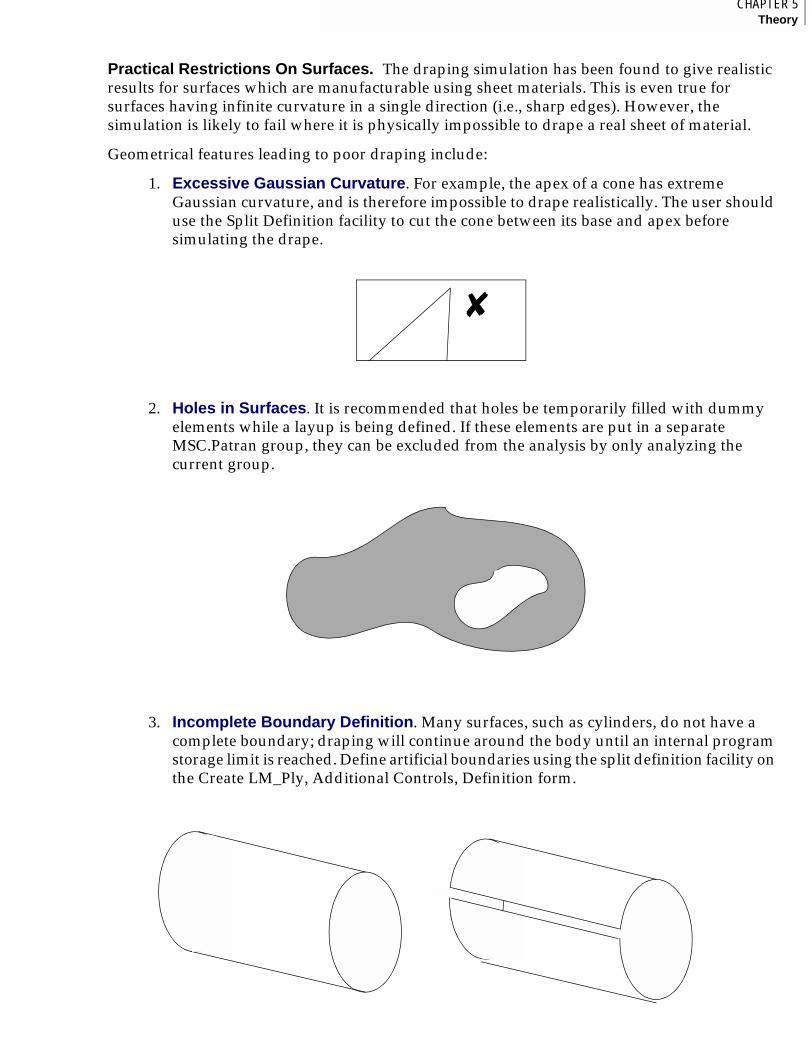
1CHAPTER 5Theory

Practical Restrictions On Surfaces. The draping simulation has been found to give realistic results for surfaces which are manufacturable using sheet materials. This is even true for surfaces having infinite curvature in a single direction (i.e., sharp edges). However, the simulation is likely to fail where it is physically impossible to drape a real sheet of material.

Geometrical features leading to poor draping include:

1. Excessive Gaussian Curvature. For example, the apex of a cone has extreme Gaussian curvature, and is therefore impossible to drape realistically. The user should use the Split Definition facility to cut the cone between its base and apex before simulating the drape.

2. Holes in Surfaces. It is recommended that holes be temporarily filled with dummy elements while a layup is being defined. If these elements are put in a separate MSC.Patran group, they can be excluded from the analysis by only analyzing the current group.

3. Incomplete Boundary Definition. Many surfaces, such as cylinders, do not have a complete boundary; draping will continue around the body until an internal program storage limit is reached. Define artificial boundaries using the split definition facility on the Create LM_Ply, Additional Controls, Definition form.

✘

4. “T” Sections. These can be draped along three separate paths. The user must make sure that the correct elements are selected, and that a consistent definition of top and bottom surfaces is maintained. This prevent plies crossing over unexpectedly.

Complicated T-section layup. General Case

1CHAPTER 5Theory

5.3 Results for Global PliesMSC.Laminate Modeler results can be rearranged to produce output for a single continuous piece of fabric rather than a local element-based ply-by-ply representation of the results. This feature is essential for proper results interpretation because a single piece of fabric may be represented by different ply numbers on different elements. The common approach to results processing is to produce results by ply number over a range of elements. This can lead to completely misleading results for typical components.The results rearrangement creates a new set of results in the database which uses the exact definition of a fabric on an element/ply-number scheme, allowing meaningful postprocessing as illustrated below.

Representative layup

PLY “1”

PLY “2”

PLY “3”

LAYER 1

LAYER 2

LAYER 3

Conventional local ply-based results.

MSC.Laminate Modeler global layer-based results.

Example

Note: Spectrum was updated for each picture so contours were assigned per plot.

Note: Results shown above are centroidal.

Global ply-based resultsLocal ply-based results

1CHAPTER 5Theory

As can be seen, the analysis references to plies can be in error. This rearrangement of results does not give “better” or “more accurate results” but provides a more realistic grouping of results. The functionality can be used to rearrange any results stored and referenced by plies in the database. For example, you could create failure criteria results using P/LAM or an in-house program, read the results into MSC.Patran, and then sort these results on the basis of global plies. The initial release of this functionality extracts and creates results at element centroids.

Some more simple examples can be used to help visualize the difference.

Results at Multiple Sections Through a Ply. This initial version of the results manipulation always tries to operate on a single result per layer.

MSC.Laminate Modeler determines how many results there are per ply by a simple formula: the number of layer results from database divided by the maximum number of plies on any element.

Note: All model dimensions are greatly exaggerated.

Inclusion or Mandrel

If the value of this = 1 then MSC.Laminate Modeler uses that single value to create the new results.

If the value is > 1 then a further calculation is done to extract what should be a reasonable value.

For example:MSC.Patran Advanced FEA

A four ply laminate shell. Three results per ply.

7

8

9

Therefore:

12/4 =3

Value to use as relevant value = mth_nint((3/2)+0.5) = 2

Results to use are starting at 2 and increasing in increments of 3

Giving Sections 2,5,8,11

4

5

6

1

2

3

10

11

12

1CHAPTER 5Theory

5.4 Composite Failure CriteriaFailure criteria for composite materials are significantly more complex than yield criteria for metals because composite materials can be strongly anisotropic and tend to fail in a number of different modes depending on their loading state and the mechanical properties of the material. While theories which reflect detailed mechanisms of failure are currently being developed, empirical criteria based on test data have been used for decades. These criteria have been incorporated in the MSC.Laminate Modeler to allow rapid evaluation of the strength of a structure according to the current industry standards. The user can also define custom criteria using PCL functions for use in specialized applications.

Nomenclature. Failure criteria compare the loading state at a point (stress or strain) with a set of values reflecting the strength of the material at that point (often referred to as the material allowables). Both loading and strength values should be reflected in the same material coordinate system. For unidirectional materials, this is typically in the direction of the fibres. However, for woven and knitted fabrics , this direction is not obvious, and might change as the material is formed to shape.

In general, the load is represented by a full stress or strain tensor having six independent components. By convention, for lamina materials the material X axis lies in the direction of the warp fibres while the Z axis lies in the through-thickness direction of the sheet. Note than in MSC.Patran, shear strains are stored in tensor rather than engineering notation, and any experimental failure strengths should reflect this.

STRESS σx,σy,σz,τxy,τyz,τxz

STRAIN εx,εy,εz,γxy,γyz,γxz

The strength of a composite can be expressed by an arbitrarily large number of values, depending on the complexity of the failure criterion. However, lamina materials, used in composites, are often assumed to be orthotropic; the through-thickness stresses or strains are ignored and it is assumed that there is negligible interaction between the different failure modes. The strength of the material can therefore be represented by seven independent variables:

TX tensile strength along the X axis 0 < TX

CX compressive strength along the X axis 0 < CX

TY tensile strength along the Y axis 0 < TY

CY compressive strength along the Y axis 0 < CY

SXY shear strength in the XY plane 0 < SXY

SYZ shear strength in the YZ plane 0 < SYZ

SXZ shear strength in the XZ plane 0 < SXZ

In the Tsai-Wu criterion, these values have been supplemented by an interaction term which reflects the interdependence of failure modes due to loading along both the X and Y material directions.

IXY interaction between X and Y directions -1< IXY <1

Note that the above values can be applied to either stress or strain.

The form of the failure criterion is typically described as a mathematical function of the above variables which reaches the value of unity at failure as follows.

Failure Index = FI (load, strength) = 1

The strength of a structure can be given as a Strength Ratio (SR), which is the ratio by which the load must be factored to just fail. (Note that the Strength Ratio is not necessarily the reciprocal of the Failure Index.) Alternatively, the Margin of Safety (MoS), where MoS = SR - 1, is used.

Maximum Criterion. This criterion is calculated by comparing the allowable load with the actual strength for each component. Mathematically, it is defined by:

FI = max (σx/TX, -σx/CX, σy/TY, -σy/CY,

abs(τxy)/SXY, abs(γyz)/SYZ, abs(γxz)/SXZ)

In this case,

SR = 1/FI

Hill Criterion. The Hill criterion was one of the first attempts to develop a single formula to account for the widely different strengths in the various principal directions:

FI = FXX σx2 + FYY σy

2 + 2 FXY σx σy + FSS τxy2

where

FXX = 1/(TX TX) if σx >= 0

1/(CX CX) if σx <0

FYY = 1/(TY TY) if σy >= 0

1/(CY CY) if σy <0

FXY = -1/(2 TX TX) if σxσy >= 0

-1/(2 CX CX) if σxσy <0

FSS = 1 / (SXY SXY)

Because this failure theory is quadratic:

SR = 1 / sqrt (FI)

In the Laminate Modeler, the Tsai-Wu criterion for in-plane loads (representing fiber failure) has been supplemented by a maximum load theory for out-of-plane shear loads (representing matrix failure):

FI = max( abs(γyz)/SYZ, abs(γxz)/SXZ)

In this case,

SR = 1/FI

For every ply, the lower of the Margins of Safety for fibre and matrix failure is calculated and displayed.

1CHAPTER 5Theory

Tsai-Wu Criterion. The Tsai-Wu failure criterion is an unashamed, empirical criterion based on the sum of the linear and quadratic invariants as follows:

Fi σi + Fij σi σj = 1 i,j = 1...6

where Fi and Fij are dependent on the material strengths. For the restrictions of lamina materials, this equation reduces to:

FI = FX σx + FY σy + FXX σx2 + FYY σy


where:

FX = 1/TX - 1/CX

FY = 1/TY - 1/CY

FXX = 1/(TX CX)

FYY = 1/(TY CY)

FXY = IXY sqrt(FXX FYY) = IXY / sqrt(TX CX TY CY)

FSS = 1 / (SXY SXY)

Because this failure theory is quadratic, the Strength Ratio (SR) = 1/FI. However, multiplying the failure criterion by SR and rearranging gives

a SR2 + b SR - 1 = 0

where

a = FXX σx2 + FYY σy


b = FX σx + FY σy

Therefore

SR = [-b + sqrt (b2 + 4a)] / 2a

In the Laminate Modeler, the Tsai-Wu criterion for in-plane loads (representing fiber failure) has been supplemented by a maximum load theory for out-of-plane shear loads (representing matrix failure):

FI = max( abs(γyz)/SYZ, abs(γxz)/SXZ )

In this case,

SR = 1/FI

For every ply, the lower of the Margins of Safety for fibre and matrix failure is calculated and displayed.

Extended Quadratic Criteria. These criterion are identical to the Tsai-Wu criterion except for the calculation of the interaction coefficient FXY which is derived rather than obtained from experimental results.

Hoffman. FXY = - 1 / (2 TX CX)

Hankinson. FXY = 0.5 / (1/(TX CX) + 1/(TY CY) - 1/SXY2)

Cowin. FXY = 1 / sqrt(TX CX TY CY) - 0.5 /SXY2

User-Defined Criterion. The user can write a custom PCL function to generate failure indices and margins of safety according to specialized failure criteria. For example, sophisticated failure criteria are being developed which incorporate a mixture of equations depending on the expected mode of failure. These could be expected to outperform simple criteria where there is a complex loading state, particularly within thick laminates.

To use this facility, the user should modify the function user() within the class p3CM_create_res_fail_user. A sample function based on the criteria of maximum loading is illustrated below. The function has input values of loading state and material strength data. The output values are the margin of safety, the critical component, and a failure index. The required function should be edited into a file “p3CM_create_res_fail_user.user.pcl.” This function must then be substituted for the default dummy function in the Laminate Modeler PCL library. To do this, save a backup copy of the existing laminate_modeler.plb, and issue the following commands in the command line:

!! LIBRARY ADD laminate_modeler.plb!! COMPILE p3CM_create_res_fail_user.user INTO laminate_modeler.plbThe PCL source code required to implement the maximum failure criteria follows as an example:CLASS p3CM_create_res_fail_user

FUNCTION user(res_array,mat_array,out_res_array)

REAL res_array() REAL mat_array() REAL out_res_array()

REAL sxx,syy,szz,sxy,syz,sxz REAL fxt,fxc,fyt,fyc,fs12,fs23,fs31 REAL margin,component,fi

REAL fi11t,fi11c,fi22t,fi22c,fi12,fi23,fi31

/* * Set input values. */ sxx = res_array(1) syy = res_array(2) szz = res_array(3) sxy = res_array(4) syz = res_array(5) sxz = res_array(6)

1CHAPTER 5Theory

fxt = mat_array(1) fxc = mat_array(2) fyt = mat_array(3) fyc = mat_array(4) fs12 = mat_array(5) fs23 = mat_array(6) fs31 = mat_array(7)

/* * Check that failure values are reasonable. */ IF ( (fxt<=0.) || @ (fxc<=0.) || @ (fyt<=0.) || @ (fyc<=0.) || @ (fs12<=0.) || @ (fs23<=0.) || @ (fs31<=0.) ) THEN

user_message(“Ack”,4,”LAMMODEL”,”Failure strength values must be > 0.0”) RETURN

END IF

/* * Initialise variables. */ margin = 0.0 component = 1.0 fi = 1.0 sys_allocate_array(out_res_array,1,3) out_res_array(1) = 0.0 out_res_array(2) = 1.0 out_res_array(3) = 1.0 /* * Calculate strength ratios for each component. */ fi11t = sxx / fxt IF( fi < fi11t )THEN fi = fi11t margin = 1. / fi - 1 component = 11 ENDIF fi11c = -sxx / fxc

IF( fi < fi11c )THEN fi = fi11c margin = 1. / fi - 1 component = -11 ENDIF fi22t = syy / fyt IF( fi < fi22t )THEN fi = fi22t margin = 1. / fi - 1 component = 22 ENDIF fi22c = -syy / fyc IF( fi < fi22c )THEN fi = fi22c margin = 1. / fi - 1 component = -22 ENDIF fi12 = mth_abs(sxy) / fs12 IF( fi < fi12 )THEN fi = fi12 margin = 1. / fi - 1 component = 12 ENDIF fi23 = mth_abs(syz) / fs23 IF( fi < fi23 )THEN fi = fi23 margin = 1. / fi - 1 component = 23 ENDIF fi31 = mth_abs(sxz) / fs31 IF( fi < fi31 )THEN fi = fi31 margin = 1. / fi - 1 component = 31 ENDIF /* * Set output values. */

out_res_array(1) = margin out_res_array(2) = component out_res_array(3) = fi

END FUNCTION

END CLASS


APPENDIX

A Bibliography

■ Bibliography

Bibliography1. Bergsma, O.K. and Huisman, J. “Deep Drawing of Fabric Reinforced Thermoplastics,”

in Brebbia, C., et al., CAD in Composite Material Technology (Southampton, Computational Mechanics, 1988).

2. Bergsma, O.K. Deep Drawing of Fabric Reinforced Thermoplastics: Simulation and Experiment (Delft University of Technology, Department of Aerospace Engineering).

3. Calladine, C. Theory of Shell Structures, Chapter 5.

4. Heisey, F.L., et al. “Three-Dimensional Pattern Drafting,” Textile Research Journal, November 1990, pp. 690-696.

5. Collier, J.R., Collier, B.J., O’Toole, G. and Sargand, S.M. “Drape Prediction by Means of Finite-Element Analysis,” J. Text. Inst., 1991, Vol. 82, No. 1, pp. 96-107.

6. Heisey, F.L., and Haller, K.D. “Fitting Woven Fabric To Surfaces in Three Dimensions,” J. Text. Inst., 1988, No. 2, pp. 250-263.

7. Hinds, B.K., McCartney, J., and Woods ,G. “Pattern Development for Three Dimensional Surfaces” (Queens University Belfast, Department of Mechanical and Manufacturing Engineering).

8. Kawabata, S. The Standardization and Analysis of Hand Evaluation, 2nd ed., (Osaka, Japan, The Textile Machinery Society of Japan, 1980).

9. Mack, C., and Taylor, H.M. “The Fitting of Woven Cloth to Surfaces,” J.Text. Inst., 1956, No. 47, pp. T477-88.

10. Mallon, P.J., O’Bradaigh, C.M., and Pipes, R.B. “Polymeric Diaphragm Forming of Complex-Curvature Thermoplastic Composite Parts,” Composites, Vol. 20, No. 1, Jan. 1989, pp.48-56.

11. Monaghan, M.R., Mallon, P.J., O’Bradaigh, C.M., and Pipes, R.B. “The Effect of Diaphragm Stiffness on the Quality of Diaphragm Formed Thermoplastic Composite Components,” The Journal of Thermoplastic Composite Materials, Vol. 3, July 1990, pp.202-215.

12. Okine, R.K. “Analysis of Forming Parts from Advanced Thermoplastic Composite Sheet Materials,” The Journal of Thermoplastic Composite Materials, Vol. 2, Jan. 1989, pp.50-77.

13. Potter, K.D. “The Influence of Accurate Stretch Data for Reinforcements on the Production of Complex Structural Mouldings -- Part 1. Deformation of Aligned Sheets & Fabrics,” Composites, July 1979, pp.161-167.

14. Potter, K.D. “The Influence of Accurate Stretch Data for Reinforcement on the Production of Complex Structural Mouldings -- Part 2. Deformation of Random Mats,” Composites, July 1979, pp. 168-173.

15. Potter, K.D. Deformation Mechanisms of Fibre Reinforcements and Their Influence on the Fabrication of Complex Structural Parts (London, Controller HMSO, 1980).

16. Robertson, R.E., et al. “Fiber Rearrangements During the Moulding of Continuous Fiber Composites. 1: Flat Cloth to a Hemisphere,” Polymer Composites, July 1981, Vol. 2, No. 3, pp. 126-131.

17. Skelton, J. Shear Of Woven Fabrics (Dedham MA, USA, FRL, 1979).

18. Smiley, A.J., and Pipes, R.B. “Analysis of the Diaphragm Forming of Continuous Fiber Reinforced Thermoplastics,” The Journal of Thermoplastic Composite Materials, Vol. 1, Oct. 1988, pp. 298-321.

1APPENDIX ABibliography

19. Stubbs, N., and Fluss, H. “A Space-truss Model for Plain-Weave Coated Fabrics,” Appl. Math. Modeling, Vol. 4, Part 1, Feb. 1980, pp. 51-58.

20. Tam, A.S., and Gutowski, T. “Ply-Slip During the Forming of Thermoplastic Composite Parts,” Journal of the ASCE Engineering Mechanics Division, Vol. 104, Part 5, Oct, 1978.

21. Testa, R.B., Stubbs, N., and Spillers, W.R. “Bilinear Model For Coated Square Fabrics,” The Journal of the ASCE Engineering Mechanics Division, Vol. 104, Part 5, Oct. 1978, pp. 1027-1042.

22. Van Der Weeen, F. “Algorithms For Draping Fabrics on Doubly-Curved Surfaces,” International Journal for Numerical Methods in Engineering, Vol. 31, 1991, pp. 1415-1426.

23. Van West, B.P., et al. The Draping and Consolidation of Commingled Fabrics (Delaware USA, Center for Composite Materials and Dept. of Mechanical Engineering, University of Delaware, 1990).

24. Wormersley, J.R. “The Application of Differential Geometry to the Study of the Deformation of Cloth Under Stress,” J. Text. Inst., 1937, pp.T97-112.

1

I N D E XMSC.Laminate Modeler User’s Guide

I N D E XMSC.Laminate Modeler User’s Guide
A
anisotropic behavior, 9anisotropy, 9automated tow placement, 11axis type, 55

energy, 55geodesic, 55planar, 55

Bbottom, 51

CCAD systems, 16, 17CADDS 5, 16CATIA, 16composites data, 5compression moulding, 10conceptual design, 12core samples, 14cross sections, 14curved shells, 124

Ddefinition, 57degree of shear, 21detailed development, 12developable surfaces, 17dome-shaped surfaces, 20doubly-curved, 15doubly-curved surfaces, 20drape simulation, 16draping

global, 127local, 126scissor, 126slide, 126

Eenergy global draping, 22, 128Euclid 3, 16excessive Gaussian curvature, 131

Ffiber angles, 129

axis method, 129planar method, 129

filament winding, 5, 11filamentary composites, 9

fabrics, 9glass fibre/polyester mixture, 9graphic fibre/epoxy resin, 9tows, 9

finite element analysis, 16flat plates, 124

GGaussian curvature, 20, 21, 124

negative, 20, 125positive, 20, 124zero, 125

geodesic global draping, 22, 127geodesic lines, 124geometry, 55global draping, 21, 22, 127

energy, 22, 128geodesic, 22, 127planar, 22, 128

Hholes in surfaces, 131

Iincomplete boundary definition, 131

INDEX

initial direction, 51initial direction vector, 52interior edge, 57

Llamination theory, 10layer, 35, 49layer materials, 43

painted, 43projected, 43scissor draped, 43slide draped, 43

layup, 35, 65layup ply table, 35layup sequence, 35layup table, 25LM_layer material, 49local draping, 21, 126

Mmanual layup, 5material generation, 43material type, 45, 50maximum strain, 43, 56, 99, 100, 101mesh, 38, 51MSC.Mvision, 16MSC.Patran COMPOSITE, 16MSC.Patran FEA, 16multiplier, 65

Nnesting software, 15non-developable, 15non-developable surfaces, 20, 49

Ooffset flag, 67offset value, 67outline design, 12

Pplanar global draping, 22, 128ply, 35ply laminate, 35

ply-book, 14pressure vessels, 23Pro/ENGINEER, 16production methods

filament winding, 5manual layup, 5resin transfer method (RTM), 5

Rreference angle, 50resin flow, 16resin transfer moulding, 5, 11RTM, 11ruled surfaces, 17

Ssaddle-shaped surfaces, 20sandwich structures, 18scissor draping, 21, 22, 126shell model, 40simulation, 5slide draping, 21, 22, 126springback, 16SRIM, 11stacking sequences, 65step length, 55, 129structural reaction injection moulding, 11

TT sections, 132thickness, 43top, 51top-hat section, 26

UUnigraphics, 16

Vview arrow, 100, 101view direction, 52

Wwaffle plate, 18

1INDEX

warp, 128warp/weft angle, 43, 56weft, 128wet layup, 10

Zzero Gaussian curvature, 17

INDEX

Documents

CONTENTSgc.nuaa.edu.cn/hangkong/doc/ziliao/MSC_PATRAN/MS… · · 2009-05-31MSC.Laminate Modeler Integration with MSC.Patran, 4 ... Create LM_Material Add Form, 45 ... are then