Embed Size (px)
Citation preview
C O N T E N T SMSC.Patran MSC.Nastran Preference Guide Volume 2: Thermal Analysis MSC.Patran MSC.Nastran Prefer-
ence Guide, Volume 2: Thermal Analysis
CHAPTER
1Overview ■ Introduction, 2
■ Using this Guide, 3
■ Thermal Material Properties, 5
■ Thermal Loads and Boundary Conditions, 6
■ Thermal Analysis, 10❑ Steady-State Analysis, 10
- Initial Conditions in Steady-State Analysis, 11❑ Transient Analysis, 12
- Initial Conditions in Transient Analysis, 13❑ Steady-State and Transient Convergence Criteria, 13
■ References, 14
2Getting Started - A Guided Exercise
■ Introduction, 16
■ Objectives, 17
■ Start MSC.Patran, 18
■ Create a Database, 19
■ Create a Rectangular Geometric Surface, 21
■ Mesh the Surface with Elements, 22
■ Modify the Mesh (Reduce the Number of Elements), 23
■ Specify Material Properties, 24
■ Assign Element Properties, 25
■ Define the Temperature at the Plate’s Bottom Edge, 27
■ Apply Heat Flux to the Plate’s Right Edge, 29
■ Apply Convection to the Plate’s Left Edge, 32
■ Perform a Steady-State Thermal Analysis, 35
■ Visualize the Thermal Results (Contour Plot), 36
3Building A Model ■ Introduction, 40
■ Finite Elements, 41
❑ Nodes, 42❑ Finite Elements, 43❑ Multi-Point Constraints, 44
■ Coordinate Frames, 45
■ Material Library, 46❑ Materials Form, 47❑ Constitutive Models, 49
■ Finite Element Properties, 51❑ Element Properties Form, 52
- Conductors and Grounded Conductors, 54- Capacitors and Grounded Capacitors, 54- Beam and Rod Elements with General Section, 54- Curved General Section Beam, 54- Curved Pipe Section Beam, 54- Tapered Section Beam, 56- Pipe Section Rod, 56- Flow Tube, 57- 2D Shell Elements, 57- 2D Axisymmetric Solid Elements, 58- 3D Solid Elements, 58
■ Loads and Boundary Conditions, 59❑ Loads and Boundary Conditions Form, 60
- Input Data Forms--Basic and Advanced Options, 63- Two Application Regions, 64- Surface Area, 65- Spatial Dependence, 65- Temperature Dependence, 65- Time Dependence, 65- Temp(Thermal), 66- Initial Temperature, 67- Applied Heat--Normal Fluxes, 68- Applied Heat--Directional Fluxes, 68- Transient Analysis, 70- Incident Thermal Vector, 71- Applied Heat--Nodal Source, 72- Applied Heat--Volumetric Generation, 72- Convection--To Ambient, 73- Convection--Flow Tube To Ambient, 75- Convection--Coupled, 78- Convection--Coupled Flow Tube, 80- Convection--Coupled Advection, 83- Convection--Duct Flow, 85- Radiation--Ambient Space, 88- Radiation--Ambient Nodes, 89- Radiation--Enclosures, 90
■ Load Cases, 93
4Running a Thermal Analysis
■ Introduction, 96
■ Review of the Analysis Form, 97❑ Analysis Form, 98
■ Translation Parameters, 101❑ Numbering Options, 103
■ Solution Types, 104❑ Solution Parameters, 105
- Radiation Parameters, 106- View Factor Parameters, 107- Transient Analysis, 109
■ Direct Text Input, 110
■ Subcase Create, 111❑ Subcase Parameters, 112
- Steady-State Subcase, 112- Transient Subcase, 115
❑ Output Requests, 116❑ Subcase Create Direct Text Input, 119
■ Subcase Select, 120
5Results Processing and Visualization
■ Overview, 122
■ Reading Thermal Analysis Results, 123❑ Read Output2 Form, 124❑ Attach XDB Form, 127
■ Results Visualization Options, 130❑ Contour Plots, 131❑ XY Plots, 133
6Read Input File ■ Review of Read Input File Form, 140
❑ Read Input File Form, 141❑ Entity Selection Form, 142❑ Define Offsets Form, 144❑ Selection of Input File, 145❑ Summary Data Form, 146❑ Reject Card Form, 147
■ Data Translated from the NASTRAN Input File, 148
■ Conflict Resolution, 149
7Example Problems ■ Overview, 152
■ Example 1 - Transient Thermal Analysis, 153
■ Example 2 - Free Convection on Printed Circuit Board, 175
■ Example 3 - Forced Air Convection on Printed Circuit Board, 185
■ Example 4 - Thermal Contact Resistance, 197
■ Example 5 - Typical Avionics Flow, 205
■ Example 6 - Radiation Enclosures, 217
■ Example 7 - Axisymmetric Flow in a Pipe, 226
■ Example 8 - Directional Heat Loads, 237
■ Example 9 - Thermal Stress Analysis from Directional Heat Loads, 246
■ Example 10 - Thermal Stress Analysis of a Bi-Metallic Plate, 252
AFiles ■ Files, 268
BError Messages ■ Error Messages, 272
CSupported Commands
■ File Management Statements, 274
■ Executive Control Statements, 275
■ Case Control Commands, 276
■ Bulk Data Entries, 277
INDEX ■ MSC.Patran MSC.Nastran Preference Guide, 281Volume 2: Thermal Analysis

MSC.Patran MSC.Nastran Preference Guide, Volume 2: Thermal Analysis
CHAPTER
1 Overview
■ Introduction
■ Using this Guide
■ Thermal Material Properties
■ Thermal Loads and Boundary Conditions
■ Thermal Analysis
■ References
1
2
1.1 IntroductionThe MSC.Patran MSC.Nastran Heat Transfer Preference supports the full range of thermal analysis capabilities available within MSC.Nastran. These capabilities include:
• conduction in one, two, and three dimensions
• fundamental convection
• one dimensional advection
• radiant exchange with space
• radiant exchange in enclosures
• specified temperatures
• surface and volumetric heat loads
• elements of thermal control systems
MSC.Nastran can span the full range of thermal analysis from system-level analysis of global energy balances to the detailed analysis associated with temperature and thermal stress limit levels. Within the integrated MSC.Patran-MSC.Nastran environment, you can simulate linear, nonlinear, steady-state, and transient thermal behavior. You can apply loads and boundary conditions either on the model’s geometry or on its finite element entities. MSC.Nastran’s sophisticated solution strategy automatically addresses the existence and extent of nonlinear behavior and adjusts the solution process accordingly.
3CHAPTER 1Overview
1
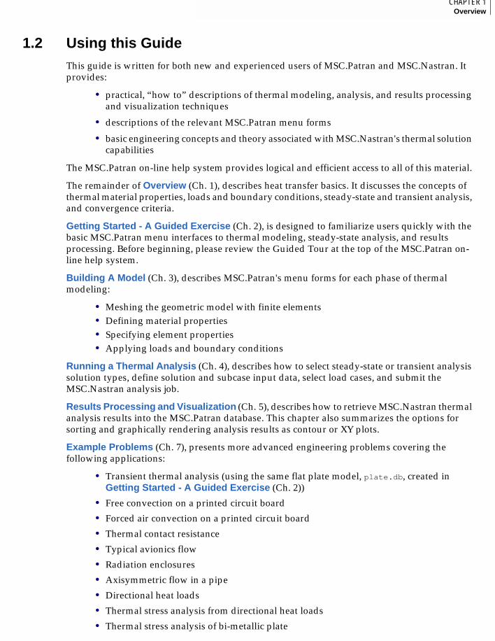
1.2 Using this GuideThis guide is written for both new and experienced users of MSC.Patran and MSC.Nastran. It provides:• practical, “how to” descriptions of thermal modeling, analysis, and results processing and visualization techniques
• descriptions of the relevant MSC.Patran menu forms
• basic engineering concepts and theory associated with MSC.Nastran's thermal solution capabilities
The MSC.Patran on-line help system provides logical and efficient access to all of this material.
The remainder of Overview (Ch. 1), describes heat transfer basics. It discusses the concepts of thermal material properties, loads and boundary conditions, steady-state and transient analysis, and convergence criteria.
Getting Started - A Guided Exercise (Ch. 2), is designed to familiarize users quickly with the basic MSC.Patran menu interfaces to thermal modeling, steady-state analysis, and results processing. Before beginning, please review the Guided Tour at the top of the MSC.Patran on-line help system.
Building A Model (Ch. 3), describes MSC.Patran's menu forms for each phase of thermal modeling:
• Meshing the geometric model with finite elements• Defining material properties• Specifying element properties• Applying loads and boundary conditions
Running a Thermal Analysis (Ch. 4), describes how to select steady-state or transient analysis solution types, define solution and subcase input data, select load cases, and submit the MSC.Nastran analysis job.
Results Processing and Visualization (Ch. 5), describes how to retrieve MSC.Nastran thermal analysis results into the MSC.Patran database. This chapter also summarizes the options for sorting and graphically rendering analysis results as contour or XY plots.
Example Problems (Ch. 7), presents more advanced engineering problems covering the following applications:
• Transient thermal analysis (using the same flat plate model, plate.db, created in Getting Started - A Guided Exercise (Ch. 2))
• Free convection on a printed circuit board
• Forced air convection on a printed circuit board
• Thermal contact resistance
• Typical avionics flow
• Radiation enclosures
• Axisymmetric flow in a pipe
• Directional heat loads
• Thermal stress analysis from directional heat loads
• Thermal stress analysis of bi-metallic plate

1
4
Files (App. A), describes the files created when using the MSC.Patran MSC.Nastran thermal preference product.
Error Messages (App. B) describes general error and diagnostic messages.
Supported Commands (App. C) describes the MSC.Nastran input data used “behind the scenes,” including File Management Statements, Executive Control Statements, Case Control Commands, and Bulk Data Entries.
5CHAPTER 1Overview
1
1.3 Thermal Material PropertiesMSC.Nastran thermal material properties include thermal conductivity, constant pressure specific heat, density, dynamic viscosity, internal heat generation, and temperature range and latent heat quantities associated with phase change phenomena.Conductivity. Thermal conductivity is an intrinsic property of all materials and in the absence of any other mode of heat transfer, provides the proportionality constant between the flow of heat through a region and the temperature gradient maintained across the region (Fourier’s Law). Thermal conductivity is generally a mild function of temperature, decreasing with increasing temperature for solids and generally increasing with increasing temperature for liquids and gases. Additionally, within a solid, thermal conductivity can vary due to material orientation (anisotropy). Preferential paths for heat flow can result. MSC.Nastran allows for temperature-dependent and directionally dependent thermal conductivity.
Specific Heat and Heat Capacitance. Specific heat is another intrinsic material property. When multiplied by the volume and density of material, the quantity of interest is referred to as heat capacitance. Given a closed thermodynamic system, heat capacitance provides the proportionality constant between heat added or subtracted from the system and the resultant temperature rise or fall of the system (dq = C * dT). Since heat capacitance only multiplies the time derivative of temperature in the heat conduction equation, specific heat is usually only relevant in the solution of transient thermal phenomenon. We will note later that advection introduces a pseudo-transient flavor even in steady-state analysis and therefore the specific heat and density of the advecting fluid are needed in these calculations.
Specific heat is also slightly temperature dependent. However, in typical heat transfer problems, the largest variations in specific heat are generally attributed to materials changing phase.
Density. For the purpose of conserving mass, the density cannot be allowed to vary with temperature. Since grid points are fixed in space in MSC.Nastran thermal analysis, if the density were to change with temperature, Density*Volume would also be changing, thus altering the system mass.
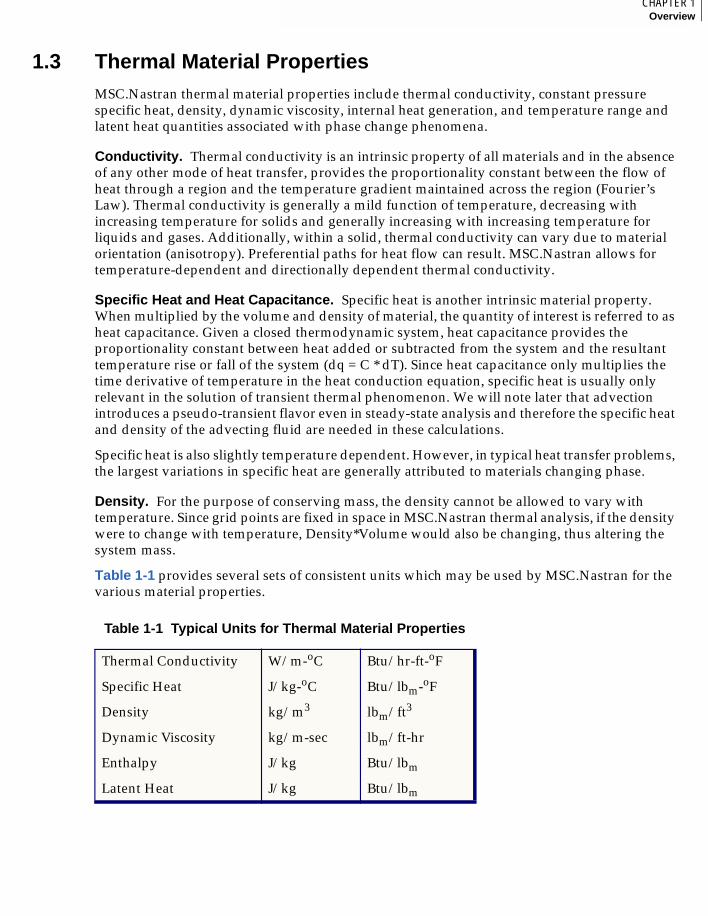
Table 1-1 provides several sets of consistent units which may be used by MSC.Nastran for the various material properties.
Table 1-1 Typical Units for Thermal Material Properties
Thermal Conductivity W/m-oC Btu/hr-ft-oF
Specific Heat J/kg-oC Btu/lbm-oF
Density kg/m3 lbm/ft3
Dynamic Viscosity kg/m-sec lbm/ft-hr
Enthalpy J/kg Btu/lbm
Latent Heat J/kg Btu/lbm
1
6
1.4 Thermal Loads and Boundary ConditionsMSC.Nastran supports a full range of thermal boundary conditions and heat loads, starting with simple temperature constraints and heat flux boundary conditions, and moving on to more complicated heat transfer mechanisms associated with convection and radiation. All of the thermal boundary conditions can be modeled as functions of time.
Thermal boundary conditions can be applied to finite element entities as well as geometric entities and include the following:
Temperature Boundary Conditions. Temperature constraints can only be applied to nodal points. Temperature constraints can be defined as constant, spatially varying, or time varying.
Normal Heat Flux. Normal heat flux is defined using the nodal, element uniform, or element variable loading operations. As with temperature boundary conditions, heat flux loads can be made to vary with space or time.
Directional Heat Flux. MSC.Nastran supports vector heat flux from a distant radiant heat source. This capability allows you to model phenomena such as diurnal or orbital heating. The required input for this capability includes:
• the magnitude of the flux vector
• the absorptivity of the surface on which the flux is being applied
• the vector components of the flux vector
The absorptivity can be dependent on temperature. The magnitude and components of the heat flux can be defined as constant, spatial varying, or time varying.
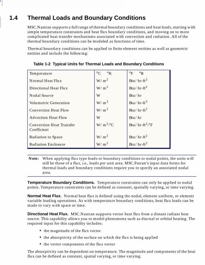
Table 1-2 Typical Units for Thermal Loads and Boundary Conditions
Temperature oC oK oF oR
Normal Heat Flux W/m2 Btu/hr-ft2
Directional Heat Flux W/m2 Btu/hr-ft2
Nodal Source W Btu/hr
Volumetric Generation W/m3 Btu/hr-ft3
Convection Heat Flow W/m2 Btu/hr-ft2
Advection Heat Flow W Btu/hr
Convection Heat Transfer Coefficient
W/m2-oC Btu/hr-ft2-oF
Radiation to Space W/m2 Btu/hr-ft2
Radiation Enclosure W/m2 Btu/hr-ft2
Note: When applying flux type loads or boundary conditions to nodal points, the units will still be those of a flux, i.e., loads per unit area. MSC.Patran’s input data forms for thermal loads and boundary conditions require you to specify an associated nodal area.
7CHAPTER 1Overview
1
Nodal Source. Heat can be applied directly on nodal points (or “grid points” in MSC.Nastran terminology). Nodal source heat can be defined as constant, spatially varying in a global sense, or time varying.Volumetric Heat Generation. Volumetric heat can be applied to one or more conduction elements and can be defined as constant, spatially varying, or time varying. The MSC.Patran MSC.Nastran interface also includes a heat generation multiplier for specifying temperature dependence. The multiplier feature is available in the input form used to specify the material property data.
Basic Convection. Basic convection boundaries can be defined. The approach to basic convection heat transfer in MSC.Nastran is to define the basic convection via a heat transfer coefficient and associated ambient temperature. The film coefficient is user specified and is available from a number of sources, including Reference 1. (p. 14). The film coefficient can be defined as a function of temperature; the ambient temperature can be defined as a function of time.
Advection, Forced Convection. Advection, forced convection, is a complicated heat transfer phenomenon that includes aspects of heat transfer as well as fluid flow. MSC.Nastran supports 1D fluid flow, which allows for energy transport due to streamwise advection and diffusion. Heat transfer between the fluid stream and the surroundings may be accounted for through a forced convection heat transfer coefficient based on locally computed Reynolds and Prandtl numbers; see Reference 1. (p. 14) and Reference 2. (p. 14) for more information on the underlying theory of this type of convection.
The input for forced convection includes:
• the mass flow rate of the fluid
• the diameter of the fluid pipe
• the material properties of the fluid
The calculation of the heat transfer coefficient between the fluid and the adjoining wall requires the specification of a film temperature. By default, this temperature will be internally calculated as the average of the temperatures of the fluid and the adjoining wall.
Additional forced convection inputs consist of the type of convection relationship used to calculate the energy transport and the method of calculating the heat transfer coefficient at the tube wall.
There are two choices with respect to the energy transport. The default method includes advection and streamwise diffusion, and its theoretical basis is the Streamwise-Upwind Petrov-Galerkin method, or SUPG.
There are also two choices for picking the method for calculating the heat transfer coefficient that applies between the fluid and the adjacent wall. The default method uses the following equation:
Eq. 1-1
The second method, chosen by picking the alternate formulation option, uses the following equation:
Eq. 1-2
h Coef ReExpr• PrExpp•=
hkd--- Coef• ReExpr• PrExpp•=
1
8
where:
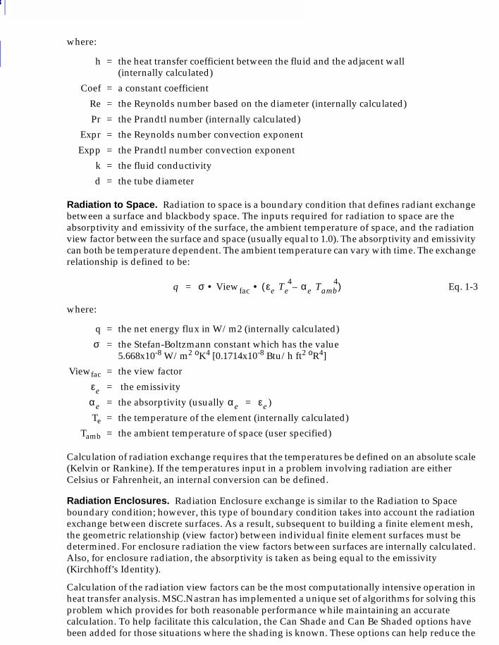
Radiation to Space. Radiation to space is a boundary condition that defines radiant exchange between a surface and blackbody space. The inputs required for radiation to space are the absorptivity and emissivity of the surface, the ambient temperature of space, and the radiation view factor between the surface and space (usually equal to 1.0). The absorptivity and emissivity can both be temperature dependent. The ambient temperature can vary with time. The exchange relationship is defined to be:
Eq. 1-3
where:
Calculation of radiation exchange requires that the temperatures be defined on an absolute scale (Kelvin or Rankine). If the temperatures input in a problem involving radiation are either Celsius or Fahrenheit, an internal conversion can be defined.
Radiation Enclosures. Radiation Enclosure exchange is similar to the Radiation to Space boundary condition; however, this type of boundary condition takes into account the radiation exchange between discrete surfaces. As a result, subsequent to building a finite element mesh, the geometric relationship (view factor) between individual finite element surfaces must be determined. For enclosure radiation the view factors between surfaces are internally calculated. Also, for enclosure radiation, the absorptivity is taken as being equal to the emissivity (Kirchhoff’s Identity).
Calculation of the radiation view factors can be the most computationally intensive operation in heat transfer analysis. MSC.Nastran has implemented a unique set of algorithms for solving this problem which provides for both reasonable performance while maintaining an accurate calculation. To help facilitate this calculation, the Can Shade and Can Be Shaded options have been added for those situations where the shading is known. These options can help reduce the
h = the heat transfer coefficient between the fluid and the adjacent wall (internally calculated)
Coef = a constant coefficient
Re = the Reynolds number based on the diameter (internally calculated)
Pr = the Prandtl number (internally calculated)
Expr = the Reynolds number convection exponent
Expp = the Prandtl number convection exponent
k = the fluid conductivity
d = the tube diameter
q = the net energy flux in W/m2 (internally calculated)
= the Stefan-Boltzmann constant which has the value5.668x10-8 W/m2 oK4 [0.1714x10⁻⁸ Btu/h ft2 oR4]
Viewfac = the view factor
= the emissivity
= the absorptivity (usually )
Te = the temperature of the element (internally calculated)
Tamb = the ambient temperature of space (user specified)
q σ Viewfac• ε e Te4 αe Tamb
4–( )•=
σ
εe
αe α e εe=

9CHAPTER 1Overview
1
calculation time for radiation enclosures. MSC.Patran also allows you to define multiple radiation enclosures. The view factors within each Radiation Enclosure will be independently calculated from the view factors of the other enclosures.In general, good view factor calculations require a reasonable surface mesh. Since the accuracy of the view factors tends to decrease as the distance between elements is reduced and becomes on the order of the element size, a mesh which prevents this sizing issue is recommended and is generally not too restrictive.
1
10
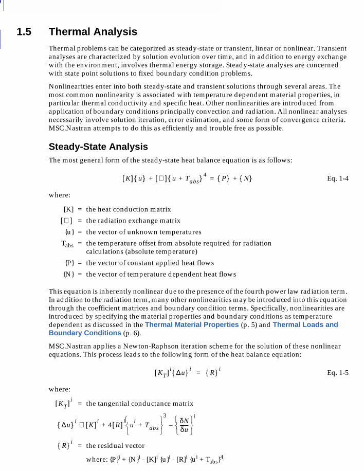
1.5 Thermal AnalysisThermal problems can be categorized as steady-state or transient, linear or nonlinear. Transient analyses are characterized by solution evolution over time, and in addition to energy exchange with the environment, involves thermal energy storage. Steady-state analyses are concerned with state point solutions to fixed boundary condition problems.
Nonlinearities enter into both steady-state and transient solutions through several areas. The most common nonlinearity is associated with temperature dependent material properties, in particular thermal conductivity and specific heat. Other nonlinearities are introduced from application of boundary conditions principally convection and radiation. All nonlinear analyses necessarily involve solution iteration, error estimation, and some form of convergence criteria. MSC.Nastran attempts to do this as efficiently and trouble free as possible.
Steady-State AnalysisThe most general form of the steady-state heat balance equation is as follows:
Eq. 1-4
where:
This equation is inherently nonlinear due to the presence of the fourth power law radiation term. In addition to the radiation term, many other nonlinearities may be introduced into this equation through the coefficient matrices and boundary condition terms. Specifically, nonlinearities are introduced by specifying the material properties and boundary conditions as temperature dependent as discussed in the Thermal Material Properties (p. 5) and Thermal Loads and Boundary Conditions (p. 6).
MSC.Nastran applies a Newton-Raphson iteration scheme for the solution of these nonlinear equations. This process leads to the following form of the heat balance equation:
Eq. 1-5
where:
[K] = the heat conduction matrix
= the radiation exchange matrix
{u} = the vector of unknown temperatures
Tabs = the temperature offset from absolute required for radiationcalculations (absolute temperature)
{P} = the vector of constant applied heat flows
{N} = the vector of temperature dependent heat flows
= the tangential conductance matrix
= the residual vector
where: {P}i + {N}i - [K]i {u}i - [R]i {ui + Tabs}4
K[ ] u{ } ℜ[ ] u Tabs+{ } 4P{ } N{ }+=+
ℜ[ ]
KT[ ] i ∆u{ } iR{ } i
=
KT[ ] i
∆u{ } iK[ ] i≅ 4 R[ ] i
ui
Tabs+
3δNδu-------
i
–+
R{ } i
11CHAPTER 1Overview
1
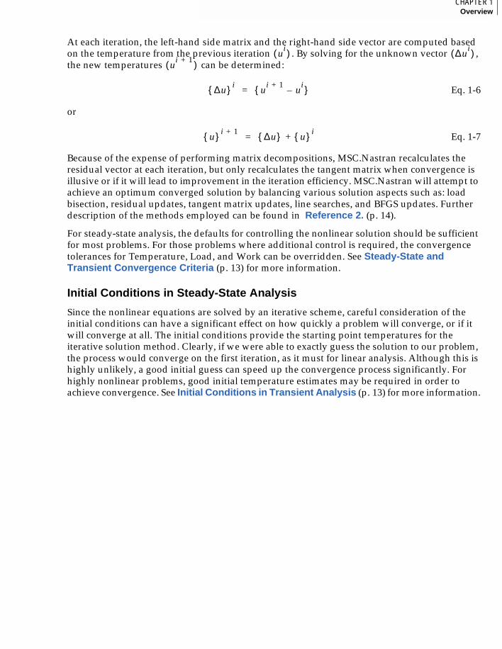
At each iteration, the left-hand side matrix and the right-hand side vector are computed based on the temperature from the previous iteration . By solving for the unknown vector , the new temperatures can be determined:Eq. 1-6
or
Eq. 1-7
Because of the expense of performing matrix decompositions, MSC.Nastran recalculates the residual vector at each iteration, but only recalculates the tangent matrix when convergence is illusive or if it will lead to improvement in the iteration efficiency. MSC.Nastran will attempt to achieve an optimum converged solution by balancing various solution aspects such as: load bisection, residual updates, tangent matrix updates, line searches, and BFGS updates. Further description of the methods employed can be found in Reference 2. (p. 14).
For steady-state analysis, the defaults for controlling the nonlinear solution should be sufficient for most problems. For those problems where additional control is required, the convergence tolerances for Temperature, Load, and Work can be overridden. See Steady-State and Transient Convergence Criteria (p. 13) for more information.
Initial Conditions in Steady-State Analysis
Since the nonlinear equations are solved by an iterative scheme, careful consideration of the initial conditions can have a significant effect on how quickly a problem will converge, or if it will converge at all. The initial conditions provide the starting point temperatures for the iterative solution method. Clearly, if we were able to exactly guess the solution to our problem, the process would converge on the first iteration, as it must for linear analysis. Although this is highly unlikely, a good initial guess can speed up the convergence process significantly. For highly nonlinear problems, good initial temperature estimates may be required in order to achieve convergence. See Initial Conditions in Transient Analysis (p. 13) for more information.
ui( ) ∆u
i( )u
i 1+( )
∆u{ } iu
i 1+u
i–{ }=
u{ } i 1+ ∆u{ } u{ } i+=
1
12
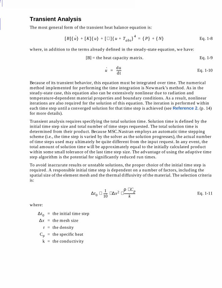
Transient AnalysisThe most general form of the transient heat balance equation is:
Eq. 1-8
where, in addition to the terms already defined in the steady-state equation, we have:
[B] = the heat capacity matrix. Eq. 1-9
Eq. 1-10
Because of its transient behavior, this equation must be integrated over time. The numerical method implemented for performing the time integration is Newmark’s method. As in the steady-state case, this equation also can be extensively nonlinear due to radiation and temperature-dependent material properties and boundary conditions. As a result, nonlinear iterations are also required for the solution of this equation. The iteration is performed within each time step until a converged solution for that time step is achieved (see Reference 2. (p. 14) for more details).
Transient analysis requires specifying the total solution time. Solution time is defined by the initial time step size and total number of time steps requested. The total solution time is determined from their product. Because MSC.Nastran employs an automatic time stepping scheme (i.e., the time step is varied by the solver as the solution progresses), the actual number of time steps used may ultimately be quite different from the input request. In any event, the total amount of solution time will be approximately equal to the initially calculated product within some small tolerance of the last time step size. The advantage of using the adaptive time step algorithm is the potential for significantly reduced run times.
To avoid inaccurate results or unstable solutions, the proper choice of the initial time step is required. A responsible initial time step is dependent on a number of factors, including the spatial size of the element mesh and the thermal diffusivity of the material. The selection criteria is:
Eq. 1-11
where:
= the initial time step
= the mesh size
r = the density
Cp = the specific heat
k = the conductivity
B[ ] u·{ } K[ ] u{ } ℜ[ ] u Tabs+{ } 4
P{ } N{ }+=+ +
u· du
dt-------=
∆ t01
10------ ∆x2
ρ Cp⋅k
----------------⋅ ⋅≅
∆t0∆x
13CHAPTER 1Overview
1
Initial Conditions in Transient AnalysisInitial conditions define the temperature starting point for a transient analysis. Every node in the problem must have an initial temperature explicitly defined. Any node that does not have an initial temperature defined will automatically have a temperature of 0.0 assigned to it. This default temperature can be changed in the Solution Parameters form for the given application, either steady-state or transient analysis.
Caution must be exercised when specifying initial conditions relative to any specified temperatures defined via a boundary condition. The initial condition temperature for these nodal points must match the (Implicit and Explicit) boundary condition temperature at time equal to zero. Failure to match these temperatures will cause an initial jump in the solution that can make convergence difficult to achieve. Fortunately, the default analysis setup will automatically enforce these temperatures to be equal at the start of the problem.
Steady-State and Transient Convergence CriteriaAs discussed previously, the solution of the nonlinear equations requires an iteration scheme. Efficient iteration schemes are highly dependent on convergence criteria and error estimation. Convergence criteria provide a means of measuring solution error relative to some predetermined acceptable level. For each iteration performed during the solution process, error levels are calculated and compared with preset tolerances. Three convergence criteria are available within MSC.Nastran that measure error based on temperature, load, and work. These criteria apply to steady-state and transient solutions alike.
Four recommendations regarding nonlinear convergence can be made:
1. For most problems, use the default criteria selection with their default tolerance values.
2. If the analysis is transient and involves any time-varying temperature boundary conditions, you must use the temperature convergence criteria.
3. Convergence may be enhanced by increasing the numerical tolerance levels from their default values.
4. For highly nonlinear transient problems, the maximum number of iterations per time step may be increased.
The defaults for controlling the nonlinear solution should be sufficient for most problems. However, for those problems requiring additional control, the convergence tolerances for Temperature, Load, and Work can be overridden. (In the solution of heat transfer problems, a convergence criteria based on WORK is realistically just a mathematical construct representing an extension of the equations used in the comparable structural solver.)

1
14
1.6 References1. Holman, J. P., Heat Transfer, Sixth Edition, McGraw-Hill Book Company, 1986.
2. Chainyk, Mike, MSC/NASTRAN Thermal Analysis User’s Guide, Version 68, The MacNeal-Schwendler Corporation, 1994.
3. Peterson, Ken (ed.), MSC/NASTRAN Encyclopedia, Online Documentation CD-ROM, The MacNeal-Schwendler Corporation, 1995.

MSC.Patran MSC.Nastran Preference Guide, Volume 2: Thermal Analysis
CHAPTER
2 Getting Started - A Guided Exercise
■ Introduction
■ Objectives
■ Start MSC.Patran
■ Create a Database
■ Create a Rectangular Geometric Surface
■ Mesh the Surface with Elements
■ Modify the Mesh (Reduce the Number of Elements)
■ Specify Material Properties
■ Assign Element Properties
■ Define the Temperature at the Plate’s Bottom Edge
■ Apply Heat Flux to the Plate’s Right Edge
■ Apply Convection to the Plate’s Left Edge
■ Perform a Steady-State Thermal Analysis
■ Visualize the Thermal Results (Contour Plot)

2
16
2.1 IntroductionThis guided exercise shows you in step-by-step fashion the basics of MSC.Nastran thermal modeling, analysis, and results visualization using MSC.Patran. By intention, the geometry is simple, as are the applied loads and boundary conditions. We will create the geometry for a rectangular metal plate, mesh it with quadrilateral elements, specify material and element properties, apply thermal loads and boundary conditions, run a steady-state thermal analysis to determine temperature distributions, and visualize the results using MSC.Patran’s postprocessor.
Before attempting this exercise, please complete the guided tour provided at the top of the MSC.Patran on-line help system. It gives you an overview of the MSC.Patran user interface, including the layout of the main form, the various application selections, the use of menus and forms, mouse picking, and basic modeling operations. Although the menu options for thermal analysis differ from those for structural analysis, MSC.Patran has a common look-and-feel across both disciplines.
17CHAPTER 2Getting Started - A Guided Exercise
2
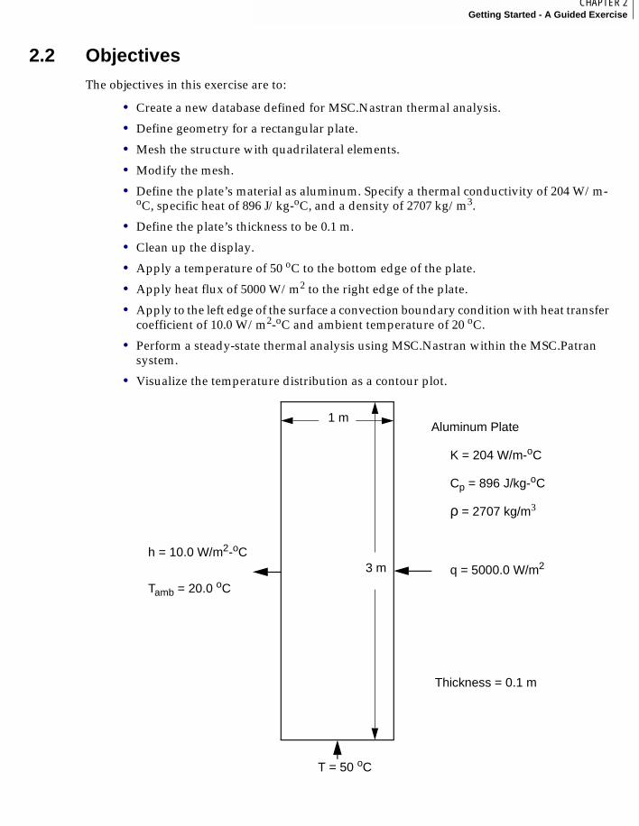
2.2 ObjectivesThe objectives in this exercise are to:
• Create a new database defined for MSC.Nastran thermal analysis.
• Define geometry for a rectangular plate.
• Mesh the structure with quadrilateral elements.
• Modify the mesh.
• Define the plate’s material as aluminum. Specify a thermal conductivity of 204 W/m-oC, specific heat of 896 J/kg-oC, and a density of 2707 kg/m3.
• Define the plate’s thickness to be 0.1 m.
• Clean up the display.
• Apply a temperature of 50 oC to the bottom edge of the plate.
• Apply heat flux of 5000 W/m2 to the right edge of the plate.
• Apply to the left edge of the surface a convection boundary condition with heat transfer coefficient of 10.0 W/m2-oC and ambient temperature of 20 oC.
• Perform a steady-state thermal analysis using MSC.Nastran within the MSC.Patran system.
• Visualize the temperature distribution as a contour plot.
1 m
3 m
Aluminum Plate
K = 204 W/m-oC
Cp = 896 J/kg-oC
ρ = 2707 kg/m3
q = 5000.0 W/m2
T = 50 oC
Tamb = 20.0 oC
h = 10.0 W/m2-oC
Thickness = 0.1 m

2
18
2.3 Start MSC.PatranTo begin the MSC.Patran modeling session from your workstation’s XTERM window, enter the command
patran
or
patran &
(if you want to run the application in the background).
19CHAPTER 2Getting Started - A Guided Exercise
2
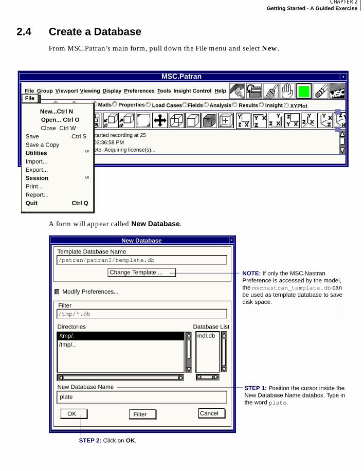
2.4 Create a DatabaseFrom MSC.Patran’s main form, pull down the File menu and select New.
A form will appear called New Database.
MSC.Patran
hp, 2
$# Session file patran.ses.01 started recording at 25$# Recorded by MSC.Patran 03:36:58 PM$# FLEXlm Initialization complete. Acquiring license(s)...
File Group Viewport Display Preferences Tools HelpInsight Control
Geometry© FEM LBCs Matls Properties© ©© © Load Cases© Fields Analysis Results Insight© ©© © XYPlot©
ViewingFile
New...Ctrl NOpen... Ctrl OClose Ctrl W
Save Ctrl SSave a Copy UtilitiesImport... Export...SessionPrint... Report...Quit Ctrl Q
ss
New Database Name
Apply Filter Cancel
New Database
/patran/patran3/template.db
Template Database Name
Change Template ...
/tmp/*.db
Filter
/tmp/..
/tmp/.
Directories Database List
OK
New Database Name
Cancel Filter
Modify Preferences...
mdl.db
plate
STEP 1: Position the cursor inside the New Database Name databox. Type in the word plate.
NOTE: If only the MSC.Nastran Preference is accessed by the model, the mscnastran_template.db can be used as template database to save disk space.
STEP 2: Click on OK.
2
20
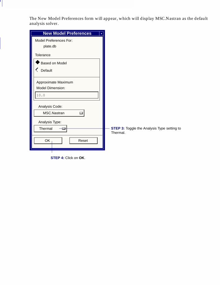
The New Model Preferences form will appear, which will display MSC.Nastran as the default analysis solver.
New Model Preferences
Model Preferences For:
plate.db
Tolerance
Based on Model
Default
Approximate Maximum
Model Dimension:
10.0
Analysis Code:
MSC.Nastran
Analysis Type:
Thermal
OK Reset
STEP 4: Click on OK.
STEP 3: Toggle the Analysis Type setting to Thermal.
◆
◆◆
21CHAPTER 2Getting Started - A Guided Exercise
2
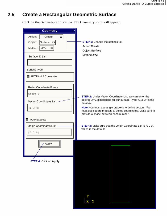
2.5 Create a Rectangular Geometric SurfaceClick on the Geometry application. The Geometry form will appear.
Geometry
Action:
Object:
Method:
Surface ID List
1
Surface Type
PATRAN 2 Convention
Refer. Coordinate Frame
Coord 0
Vector Coordinates List
<1 3 0>
Auto Execute
Origin Coordinates List
[0 0 0]
-Apply-
STEP 4: Click on Apply.
Create
Surface
XYZ
STEP 2: Under Vector Coordinate List, we can enter the desired XYZ dimensions for our surface. Type <1 3 0> in the databox.
Note: you must use angle brackets to define vectors. You must use square brackets to define coordinates. Make sure to provide a space between each number.
STEP 3: Make sure that the Origin Coordinate List is [0 0 0], which is the default.
STEP 1: Change the settings to:
Action:Create
Object:Surface
Method:XYZ
X
Y
Z
2
22
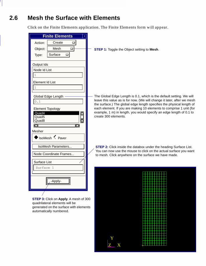
2.6 Mesh the Surface with ElementsClick on the Finite Elements application. The Finite Elements form will appear.
Finite Elements
Create Action:
Mesh Object:
Surface Type:
1
Node Id List
1
Element Id List
Output Ids
0.1
Global Edge Length
Quad5 Quad8
Element Topology
IsoMesh Paver
Mesher
IsoMesh Parameters...
Node Coordinate Frames...
Surface 1
Surface List
-Apply-
STEP 3: Click on Apply. A mesh of 300 quadrilateral elements will be generated on the surface with elements automatically numbered.
The Global Edge Length is 0.1, which is the default setting. We will leave this value as is for now. (We will change it later, after we mesh the surface.) The global edge length specifies the physical length of each element. If you are making 10 elements to comprise 1 unit (for example, 1 m) in length, you would specify an edge length of 0.1 to create 300 elements.
STEP 2: Click inside the databox under the heading Surface List. You can now use the mouse to click on the actual surface you want to mesh. Click anywhere on the surface we have made.
STEP 1: Toggle the Object setting to Mesh.
Quad4
◆◆◆
X
Y
Z
23CHAPTER 2Getting Started - A Guided Exercise
2
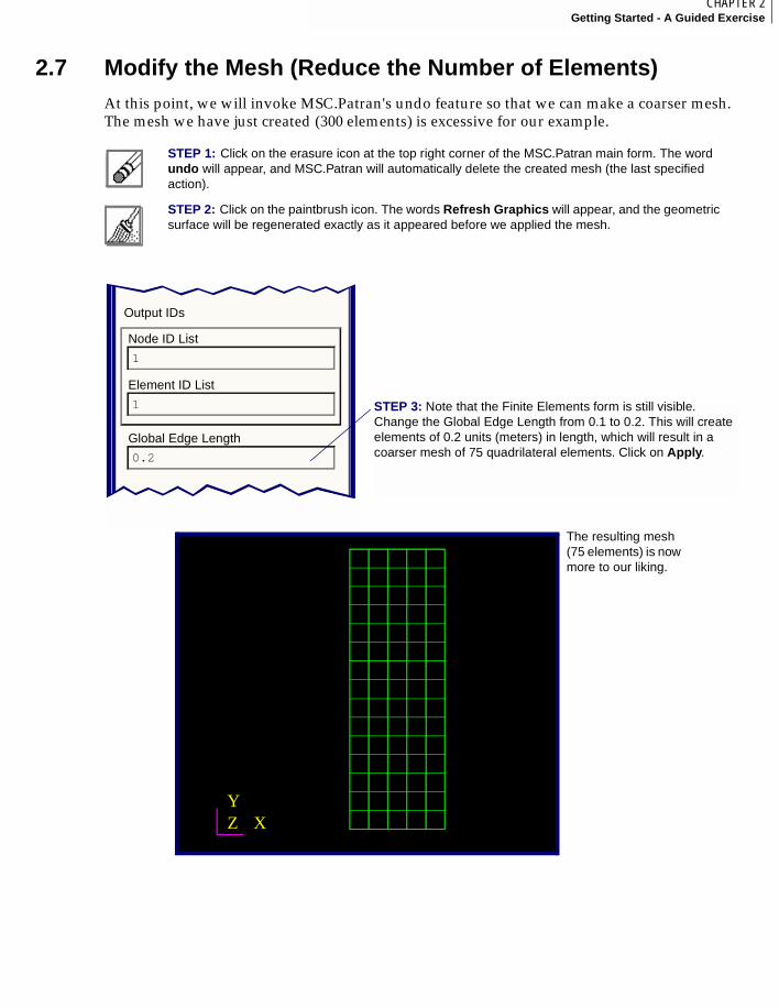
2.7 Modify the Mesh (Reduce the Number of Elements)At this point, we will invoke MSC.Patran's undo feature so that we can make a coarser mesh. The mesh we have just created (300 elements) is excessive for our example.
STEP 1: Click on the erasure icon at the top right corner of the MSC.Patran main form. The word undo will appear, and MSC.Patran will automatically delete the created mesh (the last specified action).
STEP 2: Click on the paintbrush icon. The words Refresh Graphics will appear, and the geometric surface will be regenerated exactly as it appeared before we applied the mesh.
1
Node ID List
1
Element ID List
0.2
Global Edge Length
Output IDs
STEP 3: Note that the Finite Elements form is still visible. Change the Global Edge Length from 0.1 to 0.2. This will create elements of 0.2 units (meters) in length, which will result in a coarser mesh of 75 quadrilateral elements. Click on Apply.
The resulting mesh (75 elements) is now more to our liking.
XYZ
2
24
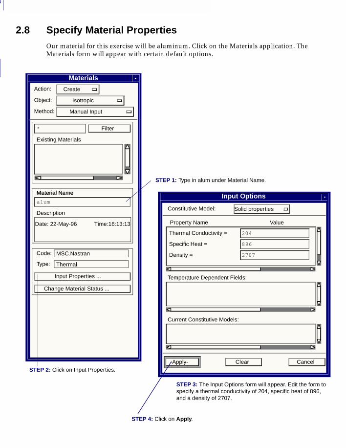
2.8 Specify Material PropertiesOur material for this exercise will be aluminum. Click on the Materials application. The Materials form will appear with certain default options.
Materials
Action: Create
Object: Isotropic
Method: Manual Input
Filter*
Existing Materials
Material Name
alum
Material Name
Description
Code:
Type:
MSC.Nastran
Thermal
Input Properties ...
Change Material Status ...
Date: 22-May-96 Time:16:13:13
STEP 2: Click on Input Properties.
STEP 4: Click on Apply.
Input Options
Constitutive Model: Solid properties
Property Name Value
Thermal Conductivity = 204
Specific Heat = 896
Density = 2707
Temperature Dependent Fields:
Current Constitutive Models:
-Apply- Clear Cancel
STEP 1: Type in alum under Material Name.
STEP 3: The Input Options form will appear. Edit the form to specify a thermal conductivity of 204, specific heat of 896, and a density of 2707.
25CHAPTER 2Getting Started - A Guided Exercise
2
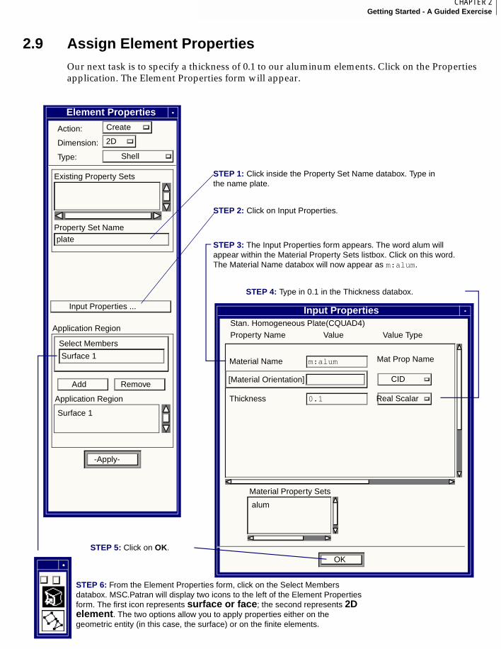
2.9 Assign Element PropertiesOur next task is to specify a thickness of 0.1 to our aluminum elements. Click on the Properties application. The Element Properties form will appear.
Element Properties Create Action:
2D Dimension:
Shell Type:
Existing Property Sets
plate Property Set Name
Input Properties ...
Surface 1
Select Members
Add Remove
Application Region
Application Region
-Apply-
Surface 1
STEP 5: Click on OK.
Input PropertiesStan. Homogeneous Plate(CQUAD4)Property Name Value Value Type
Mat Prop NameMaterial Name m:alum
CID[Material Orientation]
Real ScalarThickness 0.1
Material Property Sets
OK
alum
STEP 6: From the Element Properties form, click on the Select Members databox. MSC.Patran will display two icons to the left of the Element Properties form. The first icon represents surface or face; the second represents 2D element. The two options allow you to apply properties either on the geometric entity (in this case, the surface) or on the finite elements.
STEP 1: Click inside the Property Set Name databox. Type in the name plate.
STEP 2: Click on Input Properties.
STEP 3: The Input Properties form appears. The word alum will appear within the Material Property Sets listbox. Click on this word. The Material Name databox will now appear as m:alum.
STEP 4: Type in 0.1 in the Thickness databox.
2
26
Surface 1
Select Members
Add Remove
Application Region
Application Region
-Apply-
Surface 1
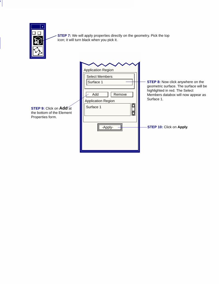
STEP 10: Click on Apply.
STEP 7: We will apply properties directly on the geometry. Pick the top icon; it will turn black when you pick it.
STEP 8: Now click anywhere on the geometric surface. The surface will be highlighted in red. The Select Members databox will now appear as Surface 1.
STEP 9: Click on Add at the bottom of the Element Properties form.
27CHAPTER 2Getting Started - A Guided Exercise
2
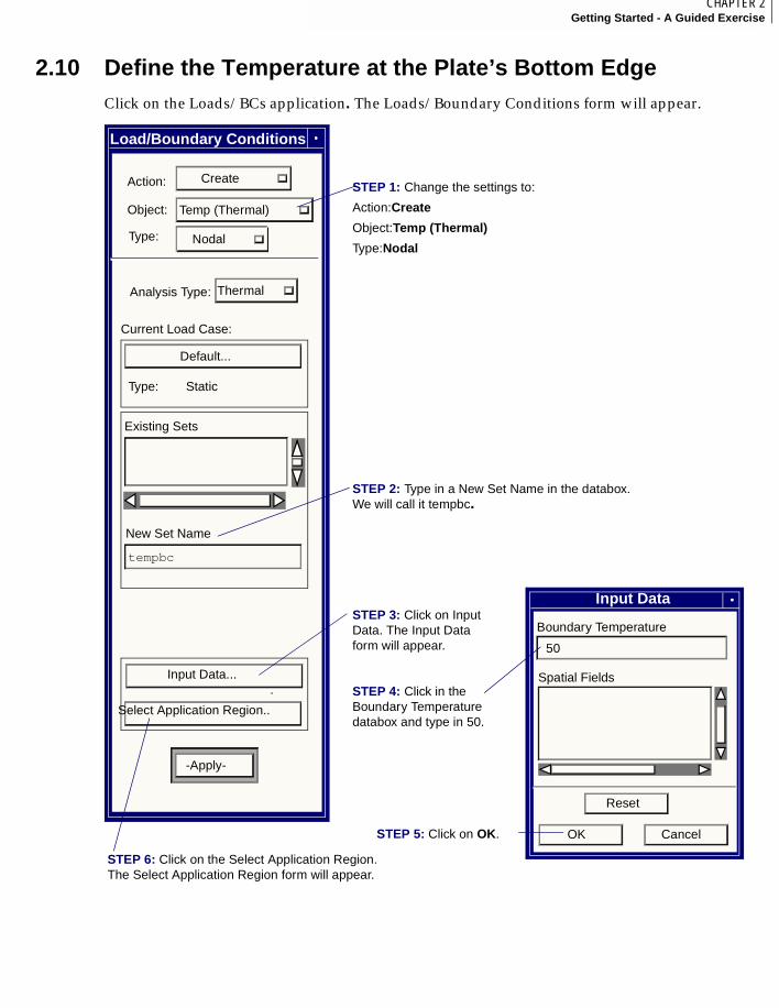
2.10 Define the Temperature at the Plate’s Bottom EdgeClick on the Loads/BCs application. The Loads/Boundary Conditions form will appear.
Input Data
Boundary Temperature
Spatial Fields
Reset
OK Cancel
50
STEP 6: Click on the Select Application Region. The Select Application Region form will appear.
Load/Boundary Conditions
Create Action:
Thermal Analysis Type:
Temp (Thermal) Object:
Nodal Type:
Default...
Type: Static
Current Load Case:
Existing Sets
tempbc
New Set Name
Input Data...
Select Application Region..
.
-Apply-
STEP 2: Type in a New Set Name in the databox. We will call it tempbc.
STEP 3: Click on Input Data. The Input Data form will appear.
STEP 4: Click in the Boundary Temperature databox and type in 50.
STEP 5: Click on OK.
STEP 1: Change the settings to:
Action:Create
Object:Temp (Thermal)
Type:Nodal
2
28
Geometry
FEM
Geometry Filter
Select Geometry Entities
Add Remove
Application Region
Application Region
OK
Select Application Region
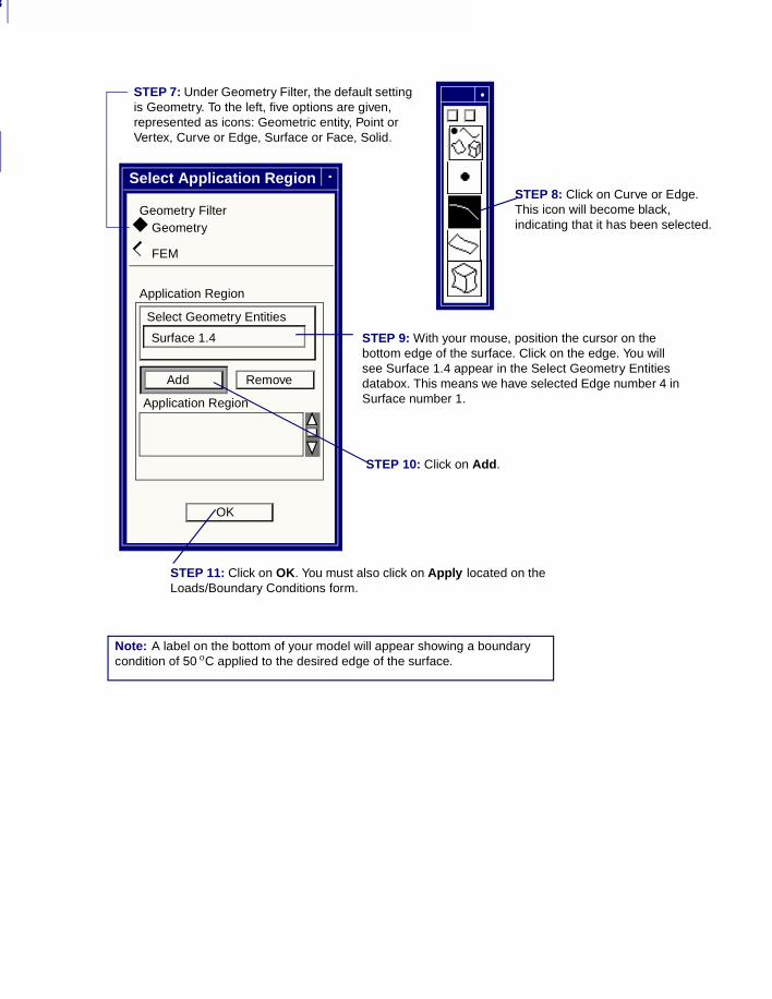
STEP 11: Click on OK. You must also click on Apply located on the Loads/Boundary Conditions form.
Surface 1.4
STEP 8: Click on Curve or Edge. This icon will become black, indicating that it has been selected.
STEP 9: With your mouse, position the cursor on the bottom edge of the surface. Click on the edge. You will see Surface 1.4 appear in the Select Geometry Entities databox. This means we have selected Edge number 4 in Surface number 1.
STEP 7: Under Geometry Filter, the default setting is Geometry. To the left, five options are given, represented as icons: Geometric entity, Point or Vertex, Curve or Edge, Surface or Face, Solid.
STEP 10: Click on Add.
Note: A label on the bottom of your model will appear showing a boundary condition of 50 oC applied to the desired edge of the surface.
◆
◆◆
29CHAPTER 2Getting Started - A Guided Exercise
2
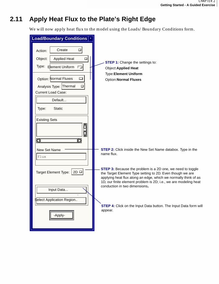
2.11 Apply Heat Flux to the Plate’s Right EdgeWe will now apply heat flux to the model using the Loads/Boundary Conditions form.
Load/Boundary Conditions
Create Action:
Thermal Analysis Type:
Applied HeatObject:
Element UniformType:
Default...
Type: Static
Current Load Case:
Existing Sets
flux
New Set Name
Input Data...
Select Application Region..
.
-Apply-
Normal FluxesOption:
Target Element Type: 2D
STEP 1: Change the settings to:
Object:Applied Heat
Type:Element Uniform
Option:Normal Fluxes
STEP 4: Click on the Input Data button. The Input Data form will appear.
STEP 2: Click inside the New Set Name databox. Type in the name flux.
STEP 3: Because the problem is a 2D one, we need to toggle the Target Element Type setting to 2D. Even though we are applying heat flux along an edge, which we normally think of as 1D, our finite element problem is 2D; i.e., we are modeling heat conduction in two dimensions.
2
30
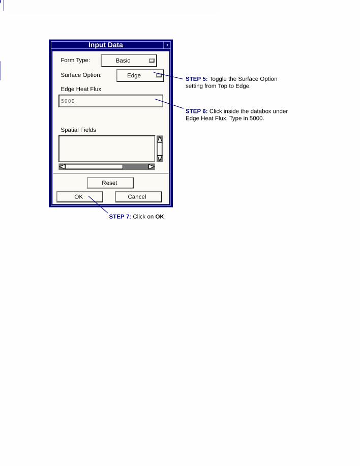
STEP 6: Click inside the databox under Edge Heat Flux. Type in 5000.
Form Type: Basic
Surface Option: Edge
Edge Heat Flux
5000
Spatial Fields
Reset
OK Cancel
Input Data
STEP 5: Toggle the Surface Option setting from Top to Edge.
STEP 7: Click on OK.
31CHAPTER 2Getting Started - A Guided Exercise
2
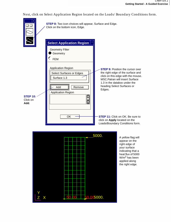
Next, click on Select Application Region located on the Loads/Boundary Conditions form.
Geometry
FEM
Geometry Filter
Select Surfaces or Edges
Add Remove
Application Region
Application Region
OK
Select Application Region
STEP 8: Two icon choices will appear, Surface and Edge. Click on the bottom icon, Edge.
Surface 1.3
STEP 9: Position the cursor over the right edge of the surface and click on this edge with the mouse. MSC.Patran will insert Surface 1.3 in the databox under the heading Select Surfaces or Edges.
STEP 11: Click on OK. Be sure to click on Apply located on the Loads/Boundary Conditions form.
STEP 10: Click on Add.
◆◆
◆
5000.
50.00XYZ 5000.50.00
A yellow flag will appear on the right edge of your surface indicating that a heat flux of 5000 W/m2 has been applied along the right edge.
2
32
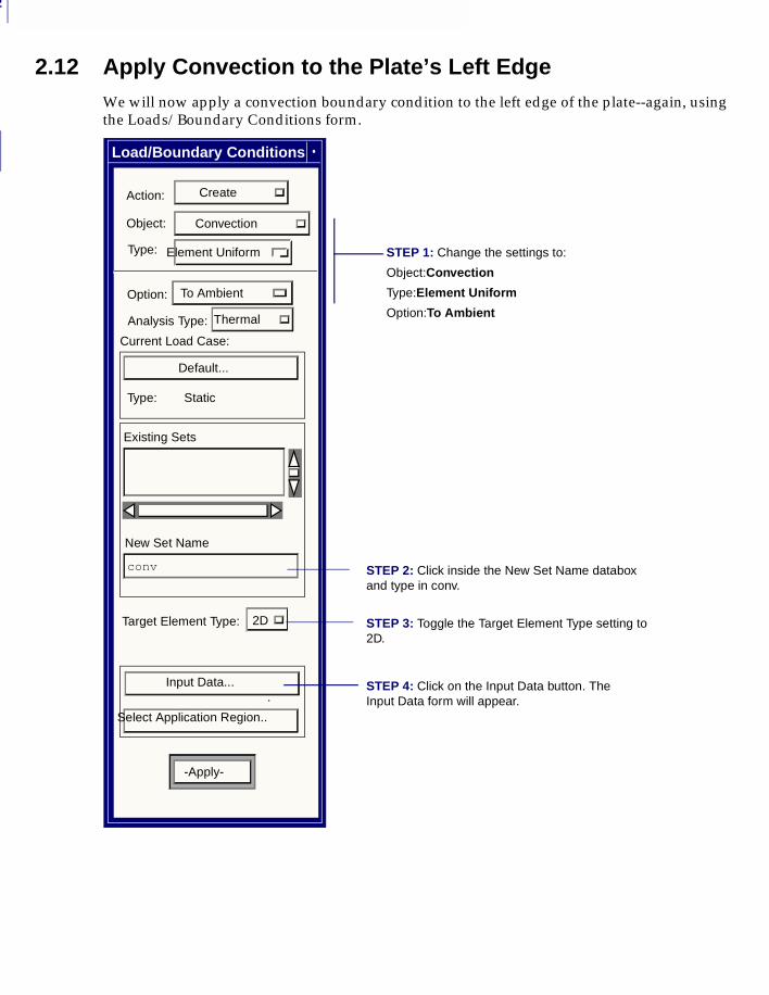
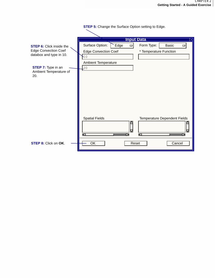
2.12 Apply Convection to the Plate’s Left EdgeWe will now apply a convection boundary condition to the left edge of the plate--again, using the Loads/Boundary Conditions form.
STEP 4: Click on the Input Data button. The Input Data form will appear.
Load/Boundary Conditions
Create Action:
Thermal Analysis Type:
ConvectionObject:
Element UniformType:
Default...
Type: Static
Current Load Case:
Existing Sets
conv
New Set Name
Input Data...
Select Application Region..
.
-Apply-
To AmbientOption:
Target Element Type: 2D
STEP 1: Change the settings to:
Object:Convection
Type:Element Uniform
Option:To Ambient
STEP 2: Click inside the New Set Name databox and type in conv.
STEP 3: Toggle the Target Element Type setting to 2D.
33CHAPTER 2Getting Started - A Guided Exercise
2
STEP 8: Click on OK.
Input DataSurface Option: Edge Form Type: Basic
Edge Convection Coef
10
* Temperature Function
Ambient Temperature
20
Spatial Fields Temperature Dependent Fields
ResetOK Cancel
STEP 5: Change the Surface Option setting to Edge.
STEP 6: Click inside the Edge Convection Coef databox and type in 10.
STEP 7: Type in an Ambient Temperature of 20.
2
34
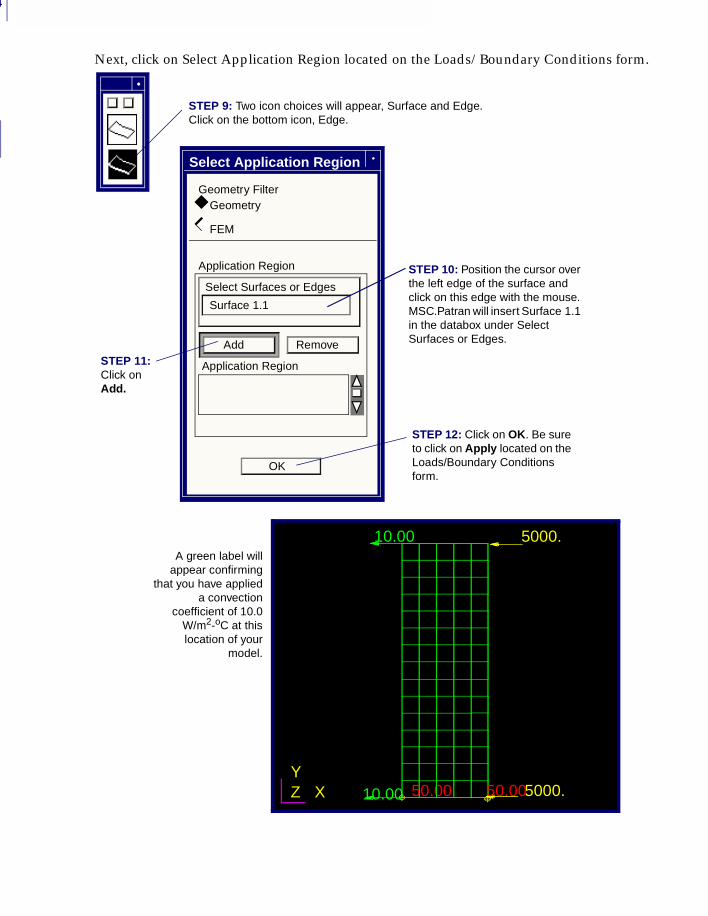
Next, click on Select Application Region located on the Loads/Boundary Conditions form.
Select Menu
Geometry
FEM
Geometry Filter
Select Surfaces or Edges
Add Remove
Application Region
Application Region
OK
Select Application Region
Surface 1.1
STEP 9: Two icon choices will appear, Surface and Edge. Click on the bottom icon, Edge.
STEP 10: Position the cursor over the left edge of the surface and click on this edge with the mouse. MSC.Patran will insert Surface 1.1 in the databox under Select Surfaces or Edges.
STEP 11: Click on Add.
STEP 12: Click on OK. Be sure to click on Apply located on the Loads/Boundary Conditions form.
◆
◆◆
A green label willappear confirming
that you have applieda convection
coefficient of 10.0W/m2-oC at thislocation of your
model.
5000.
10.00
10.00
50.00XYZ 5000.50.00
35CHAPTER 2Getting Started - A Guided Exercise
2
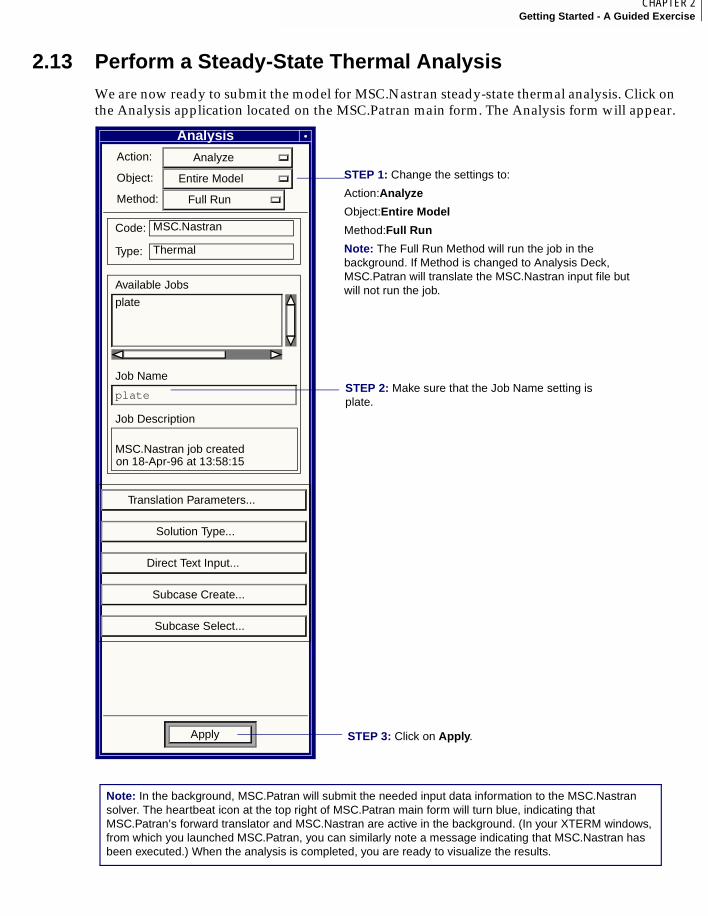
2.13 Perform a Steady-State Thermal AnalysisWe are now ready to submit the model for MSC.Nastran steady-state thermal analysis. Click on the Analysis application located on the MSC.Patran main form. The Analysis form will appear.
AnalysisAction: Analyze
Object: Entire Model
Method: Full Run
Code:
Type:
MSC.Nastran
Thermal
Available Jobs
plate
Job Name
plate
Job Description
MSC.Nastran job created
Translation Parameters...
Solution Type...
Direct Text Input...
Subcase Create...
Subcase Select...
Apply
on 18-Apr-96 at 13:58:15
STEP 1: Change the settings to:
Action:Analyze
Object:Entire Model
Method:Full Run
Note: The Full Run Method will run the job in the background. If Method is changed to Analysis Deck, MSC.Patran will translate the MSC.Nastran input file but will not run the job.
STEP 2: Make sure that the Job Name setting is plate.
Note: In the background, MSC.Patran will submit the needed input data information to the MSC.Nastran solver. The heartbeat icon at the top right of MSC.Patran main form will turn blue, indicating that MSC.Patran’s forward translator and MSC.Nastran are active in the background. (In your XTERM windows, from which you launched MSC.Patran, you can similarly note a message indicating that MSC.Nastran has been executed.) When the analysis is completed, you are ready to visualize the results.
STEP 3: Click on Apply.
2
36
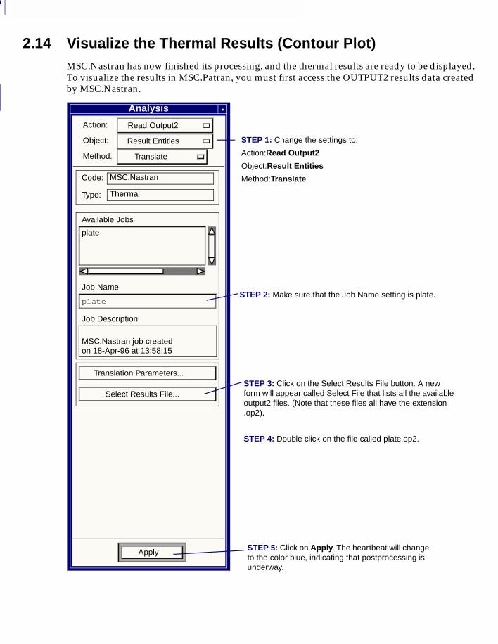
2.14 Visualize the Thermal Results (Contour Plot)MSC.Nastran has now finished its processing, and the thermal results are ready to be displayed. To visualize the results in MSC.Patran, you must first access the OUTPUT2 results data created by MSC.Nastran.
Analysis
Action: Read Output2
Object: Result Entities
Method: Translate
Code:
Type:
MSC.Nastran
Thermal
Available Jobs
plate
Job Name
plate
Job Description
MSC.Nastran job created
Translation Parameters...
Select Results File...
Apply
on 18-Apr-96 at 13:58:15
STEP 5: Click on Apply. The heartbeat will change to the color blue, indicating that postprocessing is underway.
STEP 1: Change the settings to:
Action:Read Output2
Object:Result Entities
Method:Translate
STEP 2: Make sure that the Job Name setting is plate.
STEP 3: Click on the Select Results File button. A new form will appear called Select File that lists all the available output2 files. (Note that these files all have the extension .op2).
STEP 4: Double click on the file called plate.op2.
37CHAPTER 2Getting Started - A Guided Exercise
2
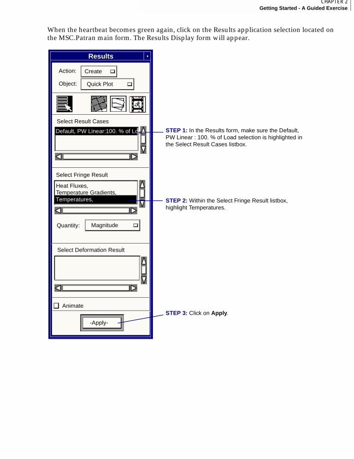
When the heartbeat becomes green again, click on the Results application selection located on the MSC.Patran main form. The Results Display form will appear.
STEP 1: In the Results form, make sure the Default, PW Linear : 100. % of Load selection is highlighted in the Select Result Cases listbox.
STEP 2: Within the Select Fringe Result listbox, highlight Temperatures.
STEP 3: Click on Apply.
Results
Default, PW Linear : 100. % of Loa
Select Result Cases
Heat Fluxes,Temperature Gradients,
Select Fringe Result
Quantity:
Select Deformation Result
-Apply-
Temperatures,
Animate
Action: Create
Object: Quick Plot
Magnitude
Default, PW Linear:100. % of Lo
Temperatures,
2
38
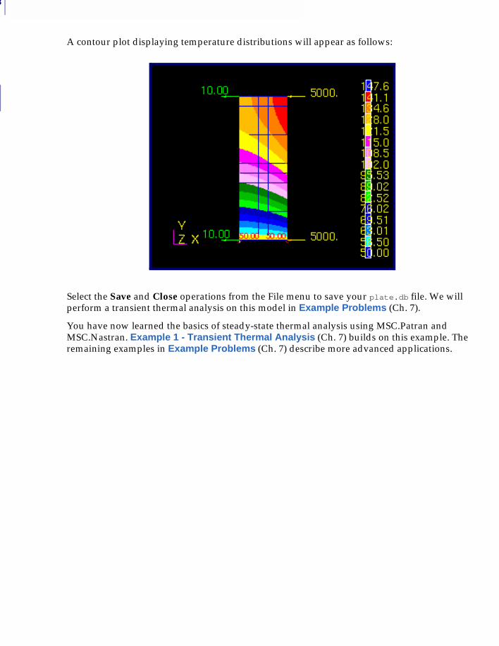
A contour plot displaying temperature distributions will appear as follows:
Select the Save and Close operations from the File menu to save your plate.db file. We will perform a transient thermal analysis on this model in Example Problems (Ch. 7).
You have now learned the basics of steady-state thermal analysis using MSC.Patran and MSC.Nastran. Example 1 - Transient Thermal Analysis (Ch. 7) builds on this example. The remaining examples in Example Problems (Ch. 7) describe more advanced applications.

MSC.Patran MSC.Nastran Preference Guide, Volume 2: Thermal Analysis
CHAPTER
3 Building A Model
■ Introduction
■ Finite Elements
■ Coordinate Frames
■ Material Library
■ Finite Element Properties
■ Loads and Boundary Conditions
■ Load Cases
3
40
3.1 IntroductionBuilding a model for heat transfer analysis can be divided into several steps:
Import or create the geometry
You can either import the geometry for your model from a CAD definition or create it within MSC.Patran. For a complete description of this process, see MSC.Patran Reference Manual, Part 2: Geometry Modeling.
Define the finite element mesh
The objective of this step is to subdivide the geometry into nodes and elements. Temperatures are calculated at the nodal points in the analysis. Heat conduction takes place within the elements. This step is described briefly in Finite Elements (p. 41). For more complete information, see MSC.Patran Reference Manual, Part 3: Finite Element Modeling.
Define material properties
In a steady-state conduction analysis, the thermal conductivity of one or more materials must be defined. In a transient analysis, the specific heat and density of the materials must also be defined. Sophisticated analyses may also require latent heat or fluid viscosity to be defined. This step is described in Material Library (p. 46).
Define element properties
The elements that define the heat conduction paths in the body can be characterized geometrically as 1D, 2D, 3D, or axisymmetric. All elements have associated material properties. In addition, one-dimensional elements must have their cross-sectional properties defined, and shell elements must have their thickness defined. This step is described in Finite Element Properties (p. 51).
Define loads and boundary conditions
Defining loads and boundary conditions is often the most difficult step in building a model for thermal analysis. In a steady-state analysis, fixed temperatures can be specified at any nodal points in the model. This applies to structural nodal points as well as ambient nodal points. In a transient analysis, temperatures specified on nodal points may be fixed or time varying.In addition to specifying temperatures, you can apply numerous other boundary conditions, including several forms of convection and radiation. Applied surface or volumetric heat flux or heat flow are described as thermal loads. Initial temperatures are specified for two primary reasons. In a transient analysis, the full mathematical description of the Fourier problem requires the statement of the initial condition, for heat transfer the beginning temperature. In a nonlinear steady-state analysis, the MSC.Nastran solver necessarily employs an iterative scheme in solving the system equations, and it requires a starting temperature to initialize the process. For more information, see Loads and Boundary Conditions (p. 59).
41CHAPTER 3Building A Model
3
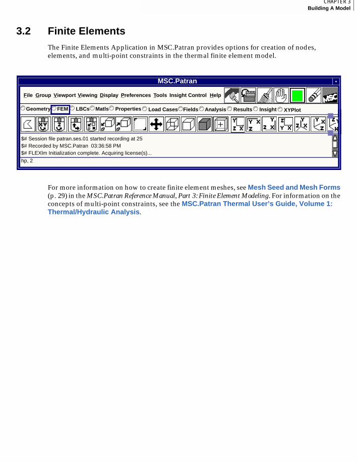
3.2 Finite ElementsThe Finite Elements Application in MSC.Patran provides options for creation of nodes, elements, and multi-point constraints in the thermal finite element model.
For more information on how to create finite element meshes, see Mesh Seed and Mesh Forms (p. 29) in the MSC.Patran Reference Manual, Part 3: Finite Element Modeling. For information on the concepts of multi-point constraints, see the MSC.Patran Thermal User’s Guide, Volume 1: Thermal/Hydraulic Analysis.
MSC.Patran
hp, 2
$# Session file patran.ses.01 started recording at 25$# Recorded by MSC.Patran 03:36:58 PM$# FLEXlm Initialization complete. Acquiring license(s)...
File Group Viewport Display Preferences Tools HelpInsight Control
Geometry© FEM LBCs Matls Properties© ©© © Load Cases© Fields Analysis Results Insight© ©© © XYPlot©
Viewing
3
42
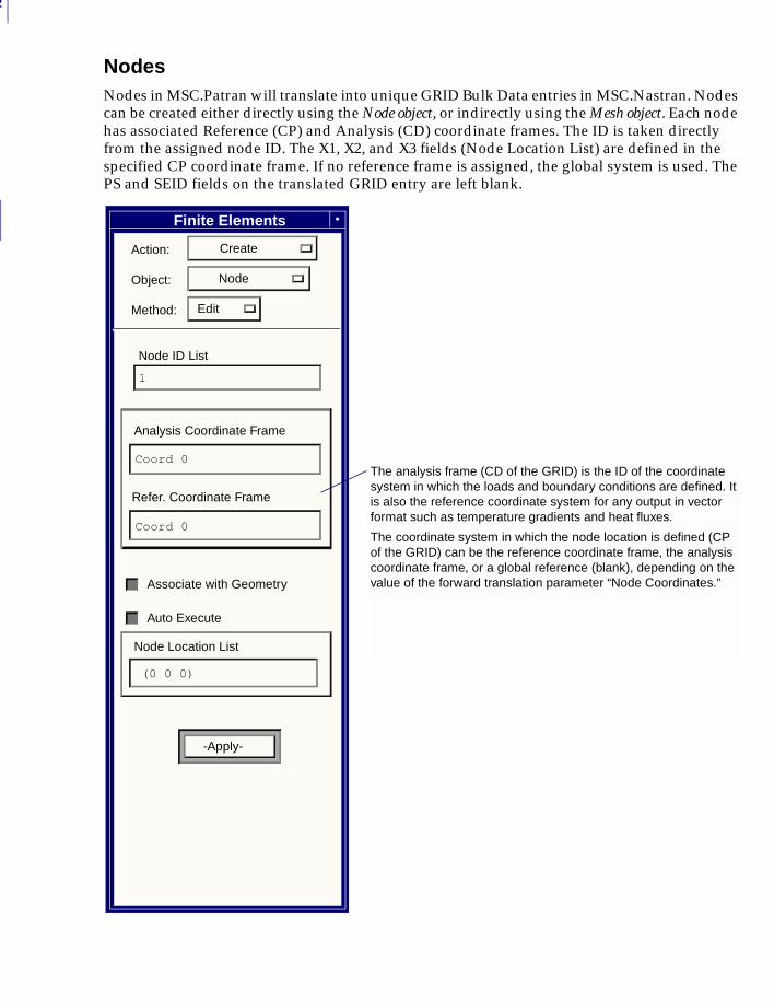
NodesNodes in MSC.Patran will translate into unique GRID Bulk Data entries in MSC.Nastran. Nodes can be created either directly using the Node object, or indirectly using the Mesh object. Each node has associated Reference (CP) and Analysis (CD) coordinate frames. The ID is taken directly from the assigned node ID. The X1, X2, and X3 fields (Node Location List) are defined in the specified CP coordinate frame. If no reference frame is assigned, the global system is used. The PS and SEID fields on the translated GRID entry are left blank.
Finite Elements
CreateAction:
NodeObject:
Edit Method:
1
Node ID List
Coord 0
Analysis Coordinate Frame
Coord 0
Refer. Coordinate Frame
Associate with Geometry
Node Location List
Auto Execute
-Apply-
The analysis frame (CD of the GRID) is the ID of the coordinate system in which the loads and boundary conditions are defined. It is also the reference coordinate system for any output in vector format such as temperature gradients and heat fluxes.
The coordinate system in which the node location is defined (CP of the GRID) can be the reference coordinate frame, the analysis coordinate frame, or a global reference (blank), depending on the value of the forward translation parameter “Node Coordinates.”
(0 0 0)
43CHAPTER 3Building A Model
3
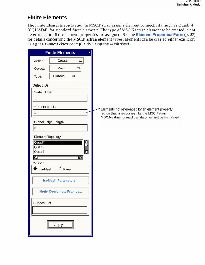
Finite ElementsThe Finite Elements application in MSC.Patran assigns element connectivity, such as Quad/4 (CQUAD4), for standard finite elements. The type of MSC.Nastran element to be created is not determined until the element properties are assigned. See the Element Properties Form (p. 52) for details concerning the MSC.Nastran element types. Elements can be created either explicitly using the Element object or implicitly using the Mesh object.
Finite Elements
CreateAction:
MeshObject:
SurfaceType:
1
Node ID List
Element ID List
Output IDs
0.1
Global Edge Length
Quad5Quad8
Element Topology
IsoMesh Paver
Mesher
IsoMesh Parameters...
Surface List
-Apply-
Elements not referenced by an element property region that is recognized by the MSC.Patran MSC.Nastran forward translator will not be translated.
Quad4
Node Coordinate Frames...
1
◆ ◆◆
3
44
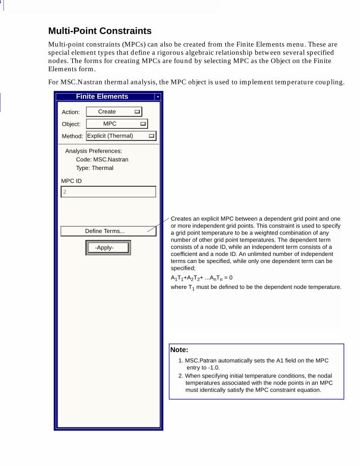
Multi-Point ConstraintsMulti-point constraints (MPCs) can also be created from the Finite Elements menu. These are special element types that define a rigorous algebraic relationship between several specified nodes. The forms for creating MPCs are found by selecting MPC as the Object on the Finite Elements form.
For MSC.Nastran thermal analysis, the MPC object is used to implement temperature coupling.
Creates an explicit MPC between a dependent grid point and one or more independent grid points. This constraint is used to specify a grid point temperature to be a weighted combination of any number of other grid point temperatures. The dependent term consists of a node ID, while an independent term consists of a coefficient and a node ID. An unlimited number of independent terms can be specified, while only one dependent term can be specified;
A1T1+A2T2+ ...AnTn = 0
where T1 must be defined to be the dependent node temperature.
Finite Elements
Action: Create
Object: MPC
Method: Explicit (Thermal)
Analysis Preferences:
Code: MSC.Nastran Type: Thermal
MPC ID
2
Define Terms...
-Apply-
Note: 1. MSC.Patran automatically sets the A1 field on the MPC
entry to -1.0.2. When specifying initial temperature conditions, the nodal
temperatures associated with the node points in an MPC must identically satisfy the MPC constraint equation.
45CHAPTER 3Building A Model
3
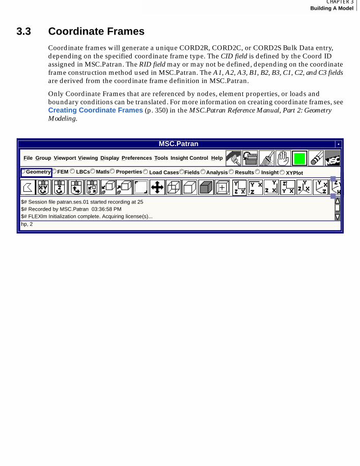
3.3 Coordinate FramesCoordinate frames will generate a unique CORD2R, CORD2C, or CORD2S Bulk Data entry, depending on the specified coordinate frame type. The CID field is defined by the Coord ID assigned in MSC.Patran. The RID field may or may not be defined, depending on the coordinate frame construction method used in MSC.Patran. The A1, A2, A3, B1, B2, B3, C1, C2, and C3 fields are derived from the coordinate frame definition in MSC.Patran.
Only Coordinate Frames that are referenced by nodes, element properties, or loads and boundary conditions can be translated. For more information on creating coordinate frames, see Creating Coordinate Frames (p. 350) in the MSC.Patran Reference Manual, Part 2: Geometry Modeling.
MSC.Patran
hp, 2
$# Session file patran.ses.01 started recording at 25$# Recorded by MSC.Patran 03:36:58 PM$# FLEXlm Initialization complete. Acquiring license(s)...
File Group Viewport Display Preferences Tools HelpInsight Control
Geometry© FEM LBCs Matls Properties© ©© © Load Cases© Fields Analysis Results Insight© ©© © XYPlot©
Viewing
3
46
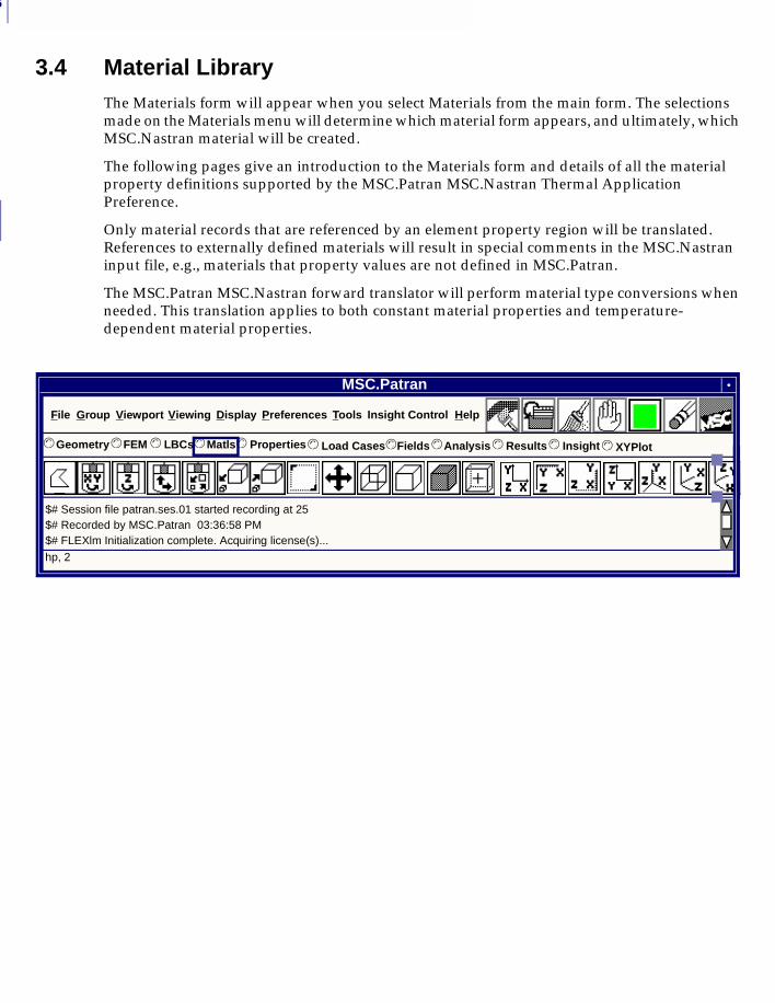
3.4 Material LibraryThe Materials form will appear when you select Materials from the main form. The selections made on the Materials menu will determine which material form appears, and ultimately, which MSC.Nastran material will be created.
The following pages give an introduction to the Materials form and details of all the material property definitions supported by the MSC.Patran MSC.Nastran Thermal Application Preference.
Only material records that are referenced by an element property region will be translated. References to externally defined materials will result in special comments in the MSC.Nastran input file, e.g., materials that property values are not defined in MSC.Patran.
The MSC.Patran MSC.Nastran forward translator will perform material type conversions when needed. This translation applies to both constant material properties and temperature-dependent material properties.
MSC.Patran
hp, 2
$# Session file patran.ses.01 started recording at 25$# Recorded by MSC.Patran 03:36:58 PM$# FLEXlm Initialization complete. Acquiring license(s)...
File Group Viewport Display Preferences Tools HelpInsight Control
Geometry© FEM LBCs Matls Properties© ©© © Load Cases© Fields Analysis Results Insight© ©© © XYPlot©
Viewing
47CHAPTER 3Building A Model
3
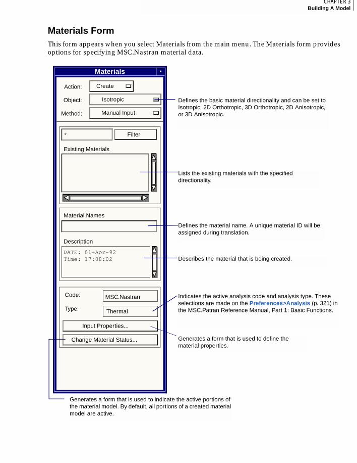
Materials FormThis form appears when you select Materials from the main menu. The Materials form provides options for specifying MSC.Nastran material data.
Defines the basic material directionality and can be set to Isotropic, 2D Orthotropic, 3D Orthotropic, 2D Anisotropic, or 3D Anisotropic.
Defines the material name. A unique material ID will be assigned during translation.
Materials
Create
Isotropic
Filter*
Existing Materials
Material Names
DATE: 01-Apr-92
Description
Code:
Type:
MSC.Nastran
Thermal
Input Properties...
Change Material Status...
Action:
Object:
Lists the existing materials with the specified directionality.
Describes the material that is being created.
Generates a form that is used to define the material properties.
Indicates the active analysis code and analysis type. These selections are made on the Preferences>Analysis (p. 321) in the MSC.Patran Reference Manual, Part 1: Basic Functions.
Generates a form that is used to indicate the active portions of the material model. By default, all portions of a created material model are active.
Method: Manual Input
Time: 17:08:02
3
48
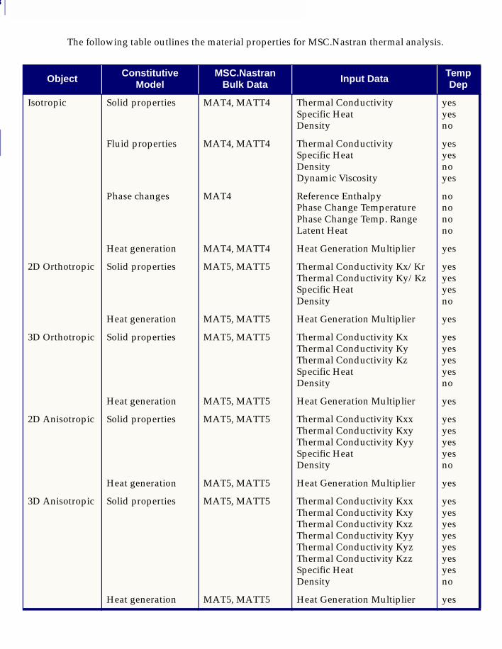
The following table outlines the material properties for MSC.Nastran thermal analysis.
Object Constitutive Model
MSC.NastranBulk Data Input Data Temp
Dep
Isotropic Solid properties MAT4, MATT4 Thermal ConductivitySpecific HeatDensity
yesyesno
Fluid properties MAT4, MATT4 Thermal ConductivitySpecific HeatDensityDynamic Viscosity
yesyesnoyes
Phase changes MAT4 Reference EnthalpyPhase Change TemperaturePhase Change Temp. RangeLatent Heat
nononono
Heat generation MAT4, MATT4 Heat Generation Multiplier yes
2D Orthotropic Solid properties MAT5, MATT5 Thermal Conductivity Kx/KrThermal Conductivity Ky/KzSpecific HeatDensity
yesyesyesno
Heat generation MAT5, MATT5 Heat Generation Multiplier yes
3D Orthotropic Solid properties MAT5, MATT5 Thermal Conductivity KxThermal Conductivity KyThermal Conductivity KzSpecific HeatDensity
yesyesyesyesno
Heat generation MAT5, MATT5 Heat Generation Multiplier yes
2D Anisotropic Solid properties MAT5, MATT5 Thermal Conductivity KxxThermal Conductivity KxyThermal Conductivity KyySpecific HeatDensity
yesyesyesyesno
Heat generation MAT5, MATT5 Heat Generation Multiplier yes
3D Anisotropic Solid properties MAT5, MATT5 Thermal Conductivity KxxThermal Conductivity KxyThermal Conductivity KxzThermal Conductivity KyyThermal Conductivity KyzThermal Conductivity KzzSpecific HeatDensity
yesyesyesyesyesyesyesno
Heat generation MAT5, MATT5 Heat Generation Multiplier yes
49CHAPTER 3Building A Model
3
Constitutive ModelsThe material properties for isotropic materials are divided into different categories called constitutive models, as follows:
For a single material, you only need to define the constitutive models and properties necessary for the particular analysis. For example, in a steady-state analysis of a simple solid, you need only define the thermal conductivity. The phase changes and heat generation constitutive models need to be defined only when these effects are present in the analysis.
Solid Properties. Thermal conductivities may be defined for isotropic, orthotropic, and anisotropic materials. When the 2D orthotropic material is used in an axisymmetric analysis, the conductivity Kr applies to the radial direction and the conductivity Kz is along the axis of symmetry. The conductivities may be defined as functions of temperature by creating temperature-dependent functions in the Fields application and then referencing these functions on the Materials form.
Density and specific heat define the heat capacity of the body and are needed only in transient analysis.
Fluid Properties. The dynamic viscosity is used in the calculation of the Reynolds (Re) and Prandtl (Pr) number in forced convection/advection applications and applies only to the Flow Tube element. The fluid specific heat, thermal conductivity, and density are also required for the formulation of the advective Streamwise Upwind Petrov Galerkin (SUPG) elements. This is the case even for steady-state analysis.
Recall Eq. 3-1
Phase Changes1. To model a phase change, you need to specify the latent heat and a finite temperature range over which the phase change is to occur. You also need to specify the lower boundary of the transition temperature as well as the reference enthalpy. The reference enthalpy is defined as the enthalpy corresponding to a zero temperature if the heat capacity Cp is a constant. If the heat capacity is temperature dependent, then the enthalpy must be defined at the lowest temperature value in the tabular field.
For pure materials, the temperature range over which the phase change takes place can be quite small, whereas for solutions or alloys the range can be quite large. Numerically, the wider the range the better. It is not recommended to make this range less than a few degrees.
Solid Properties (p. 49)
Fluid Properties (p. 49)
Phase Changes (p. 49)
Heat Generation1 (p. 50)
1If you define this constitutive model, you must also define a constitutive model for Solid Properties.
ReDVρ
µ-------------= and PrCpµ
K-----------=

3
50
Heat Generation1. The heat generation multiplier allows the definition of a temperature-dependent rate of volumetric heat generation to be defined. Usually a temperature-dependent function will be defined in Fields and selected on the Materials form. The value defined by this field will multiply the rate of heat generation defined on the Applied Heat, Volumetric Generation LBC. If the heat generation is not temperature dependent, only the Volumetric Generation LBC needs to be defined.
51CHAPTER 3Building A Model
3
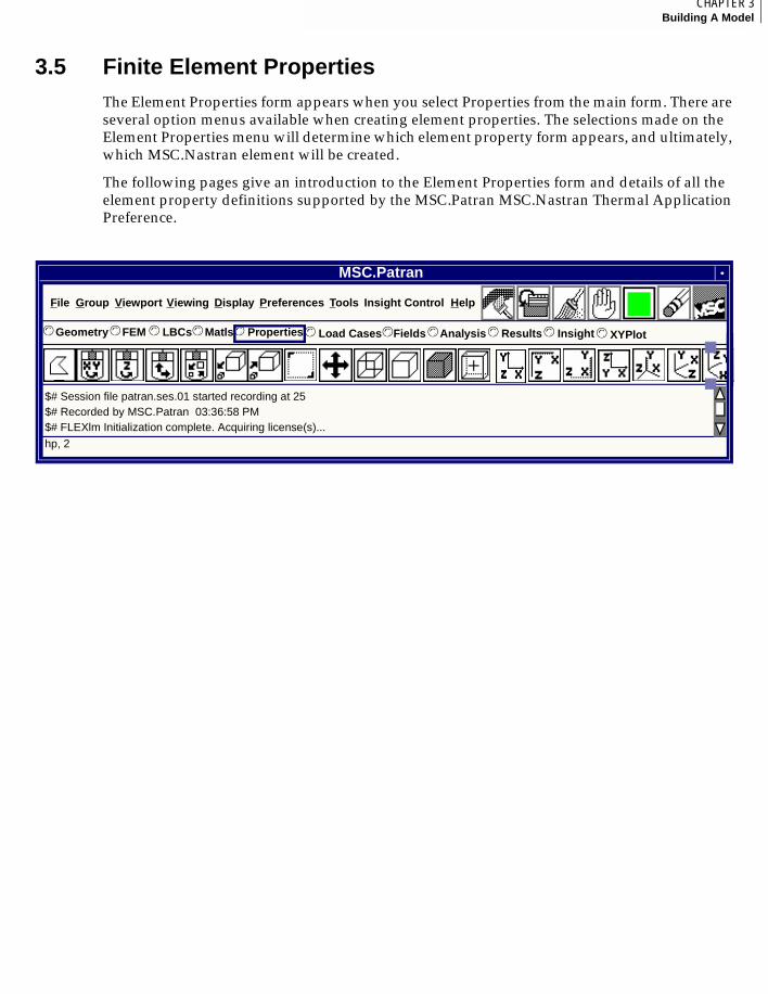
3.5 Finite Element PropertiesThe Element Properties form appears when you select Properties from the main form. There are several option menus available when creating element properties. The selections made on the Element Properties menu will determine which element property form appears, and ultimately, which MSC.Nastran element will be created.
The following pages give an introduction to the Element Properties form and details of all the element property definitions supported by the MSC.Patran MSC.Nastran Thermal Application Preference.
MSC.Patran
hp, 2
$# Session file patran.ses.01 started recording at 25$# Recorded by MSC.Patran 03:36:58 PM$# FLEXlm Initialization complete. Acquiring license(s)...
File Group Viewport Display Preferences Tools HelpInsight Control
Geometry© FEM LBCs Matls Properties© ©© © Load Cases© Fields Analysis Results Insight© ©© © XYPlot©
Viewing
3
52
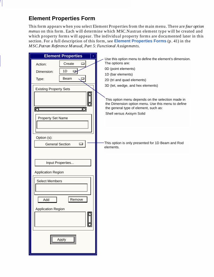
Element Properties FormThis form appears when you select Element Properties from the main menu. There are four option menus on this form. Each will determine which MSC.Nastran element type will be created and which property forms will appear. The individual property forms are documented later in this section. For a full description of this form, see Element Properties Forms (p. 41) in the MSC.Patran Reference Manual, Part 5: Functional Assignments.
Use this option menu to define the element’s dimension. The options are:
0D (point elements)
1D (bar elements)
2D (tri and quad elements)
3D (tet, wedge, and hex elements)
This option menu depends on the selection made in the Dimension option menu. Use this menu to define the general type of element, such as:
Shell versus Axisym Solid
This option is only presented for 1D Beam and Rod elements.
Element Properties
CreateAction:
1DDimension:
Type:
Option (s):
Existing Property Sets
Select Members
Add Remove
Application Region
Application Region
Apply
General Section
Beam
Input Properties...
Property Set Name
53CHAPTER 3Building A Model
3
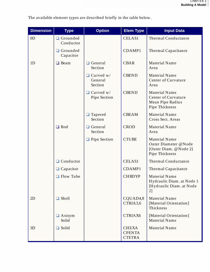
The available element types are described briefly in the table below.
Dimension Type Option Elem Type Input Data
0D ❏ Grounded Conductor
CELAS1 Thermal Conductance
❏ Grounded Capacitor
CDAMP1 Thermal Capacitance
1D ❏ Beam ❏ General Section
CBAR Material NameArea
❏ Curved w/ General Section
CBEND Material NameCenter of CurvatureArea
❏ Curved w/ Pipe Section
CBEND Material NameCenter of CurvatureMean Pipe RadiusPipe Thickness
❏ Tapered Section
CBEAM Material NameCross Sect. Areas
❏ Rod ❏ General Section
CROD Material NameArea
❏ Pipe Section CTUBE Material NameOuter Diameter @ Node[Outer Diam. @ Node 2]Pipe Thickness
❏ Conductor CELAS1 Thermal Conductance
❏ Capacitor CDAMP1 Thermal Capacitance
❏ Flow Tube CHBDYP Material NameHydraulic Diam. at Node 1[Hydraulic Diam. at Node 2]
2D ❏ Shell CQUAD4,8CTRIA3,6
Material Name[Material Orientation]Thickness
❏ Axisym Solid
CTRIAX6 [Material Orientation]Material Name
3D ❏ Solid CHEXACPENTACTETRA
Material Name
3
54
Conductors and Grounded Conductors
These elements provide a simple conductance link between either two nodes in the model or a node and a zero temperature heat sink. The only property to be defined is the thermal conductance of the link. This value can either be real or a reference to an existing field definition.
Capacitors and Grounded Capacitors
These elements provide a simple thermal capacitance link between either two nodes in the model or a node and a zero temperature heat sink. The only property to be defined is the thermal capacitance of the link. This value can either be real or a reference to an existing field definition.
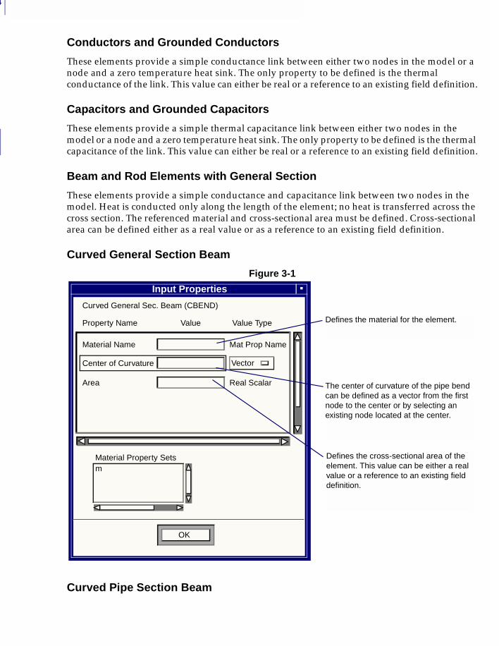
Beam and Rod Elements with General Section
These elements provide a simple conductance and capacitance link between two nodes in the model. Heat is conducted only along the length of the element; no heat is transferred across the cross section. The referenced material and cross-sectional area must be defined. Cross-sectional area can be defined either as a real value or as a reference to an existing field definition.
Curved General Section Beam
Figure 3-1
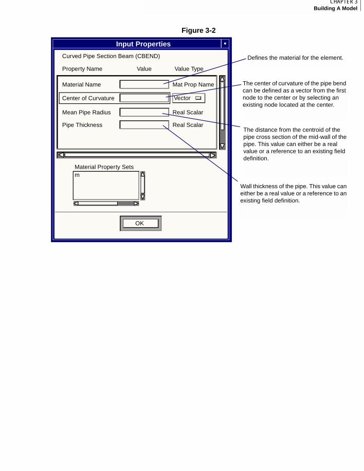
Curved Pipe Section Beam
Defines the material for the element.
The center of curvature of the pipe bend can be defined as a vector from the first node to the center or by selecting an existing node located at the center.
Defines the cross-sectional area of the element. This value can be either a real value or a reference to an existing field definition.
Input Properties
Curved General Sec. Beam (CBEND)
Property Name Value Value Type
Material Name
Center of Curvature
Area
Mat Prop Name
Real Scalar
OK
Vector
Material Property Setsm
55CHAPTER 3Building A Model
3
Figure 3-2
Defines the material for the element.
The center of curvature of the pipe bend can be defined as a vector from the first node to the center or by selecting an existing node located at the center.
The distance from the centroid of the pipe cross section of the mid-wall of the pipe. This value can either be a real value or a reference to an existing field definition.
Wall thickness of the pipe. This value can either be a real value or a reference to an existing field definition.
Input Properties
Curved Pipe Section Beam (CBEND)
Property Name Value Value Type
Material Name
Center of Curvature
Mean Pipe Radius
Mat Prop Name
Real Scalar
OK
Vector
Material Property Setsm
Pipe Thickness Real Scalar
3
56
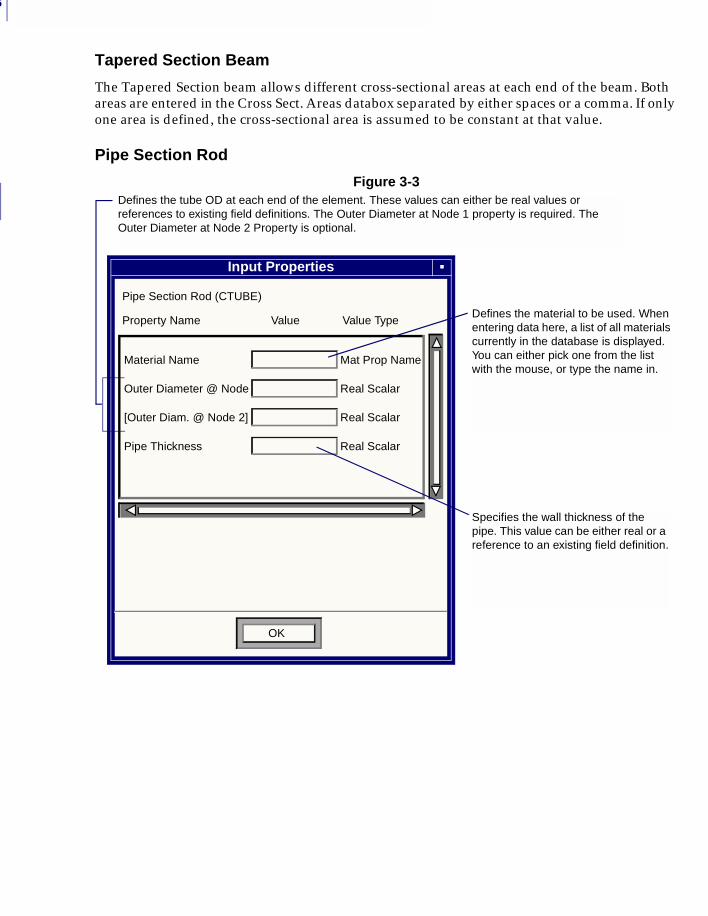
Tapered Section Beam
The Tapered Section beam allows different cross-sectional areas at each end of the beam. Both areas are entered in the Cross Sect. Areas databox separated by either spaces or a comma. If only one area is defined, the cross-sectional area is assumed to be constant at that value.
Pipe Section Rod
Figure 3-3
Defines the material to be used. When entering data here, a list of all materials currently in the database is displayed. You can either pick one from the list with the mouse, or type the name in.
Defines the tube OD at each end of the element. These values can either be real values or references to existing field definitions. The Outer Diameter at Node 1 property is required. The Outer Diameter at Node 2 Property is optional.
Input Properties
Pipe Section Rod (CTUBE)
Property Name Value Value Type
Material Name
Outer Diameter @ Node Real Scalar
[Outer Diam. @ Node 2]
Pipe Thickness
Mat Prop Name
Real Scalar
OK
Real Scalar
Specifies the wall thickness of the pipe. This value can be either real or a reference to an existing field definition.
57CHAPTER 3Building A Model
3
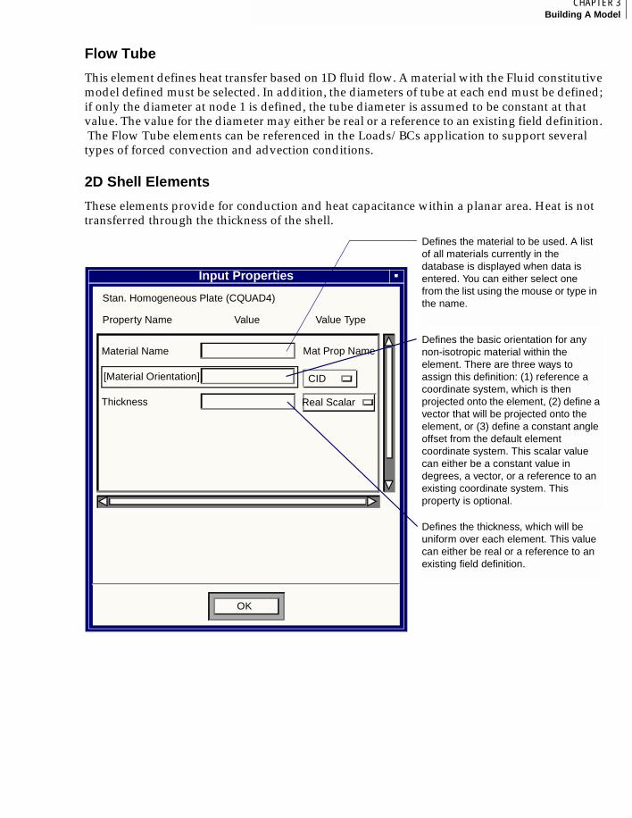
Flow Tube
This element defines heat transfer based on 1D fluid flow. A material with the Fluid constitutive model defined must be selected. In addition, the diameters of tube at each end must be defined; if only the diameter at node 1 is defined, the tube diameter is assumed to be constant at that value. The value for the diameter may either be real or a reference to an existing field definition. The Flow Tube elements can be referenced in the Loads/BCs application to support several types of forced convection and advection conditions.
2D Shell Elements
These elements provide for conduction and heat capacitance within a planar area. Heat is not transferred through the thickness of the shell.
Defines the material to be used. A list of all materials currently in the database is displayed when data is entered. You can either select one from the list using the mouse or type in the name.
Defines the thickness, which will be uniform over each element. This value can either be real or a reference to an existing field definition.
Input Properties
Stan. Homogeneous Plate (CQUAD4)
Property Name Value Value Type
Material Name
[Material Orientation]
Thickness
OK
CID
Real Scalar
Mat Prop NameDefines the basic orientation for any non-isotropic material within the element. There are three ways to assign this definition: (1) reference a coordinate system, which is then projected onto the element, (2) define a vector that will be projected onto the element, or (3) define a constant angle offset from the default element coordinate system. This scalar value can either be a constant value in degrees, a vector, or a reference to an existing coordinate system. This property is optional.
3
58
2D Axisymmetric Solid Elements
These elements are used to model heat conduction in a body that is symmetric about a particular coordinate axis. When defining the model with MSC.Patran, this axis must be the global z-axis and the radial axis must be the global x-axis (i.e., the elements must lie in the x-z plane). The only element property required is the material. An optional material orientation allows you to define the orientation for any non-isotropic material within the element.
You can specify temperature boundary conditions, initial temperatures, and nodal and volumetric heat loads on the element’s boundaries or interior. You can specify exchange type boundary conditions (convection and radiation) on the boundaries of the geometry.
With Version 68 of MSC.Nastran, if convection or radiation boundary conditions are applied to 6-node triangular axisymmetric elements, the heat flux results associated with these elements cannot be postprocessed in MSC.Patran. To postprocess boundary heat fluxes, the 3-node triangular axisymmetric elements must be used instead.
3D Solid Elements
These elements provide for conduction and heat capacitance within a volume. A material property must be selected to define the thermal conductivity, density, and specific heat.
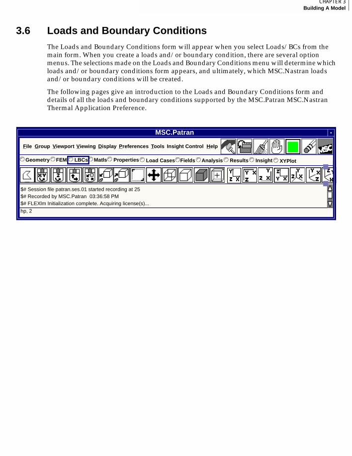
59CHAPTER 3Building A Model
3
3.6 Loads and Boundary ConditionsThe Loads and Boundary Conditions form will appear when you select Loads/BCs from the main form. When you create a loads and/or boundary condition, there are several option menus. The selections made on the Loads and Boundary Conditions menu will determine which loads and/or boundary conditions form appears, and ultimately, which MSC.Nastran loads and/or boundary conditions will be created.
The following pages give an introduction to the Loads and Boundary Conditions form and details of all the loads and boundary conditions supported by the MSC.Patran MSC.Nastran Thermal Application Preference.
MSC.Patran
hp, 2
$# Session file patran.ses.01 started recording at 25$# Recorded by MSC.Patran 03:36:58 PM$# FLEXlm Initialization complete. Acquiring license(s)...
File Group Viewport Display Preferences Tools HelpInsight Control
Geometry© FEM LBCs Matls Properties© ©© © Load Cases© Fields Analysis Results Insight© ©© © XYPlot©
Viewing
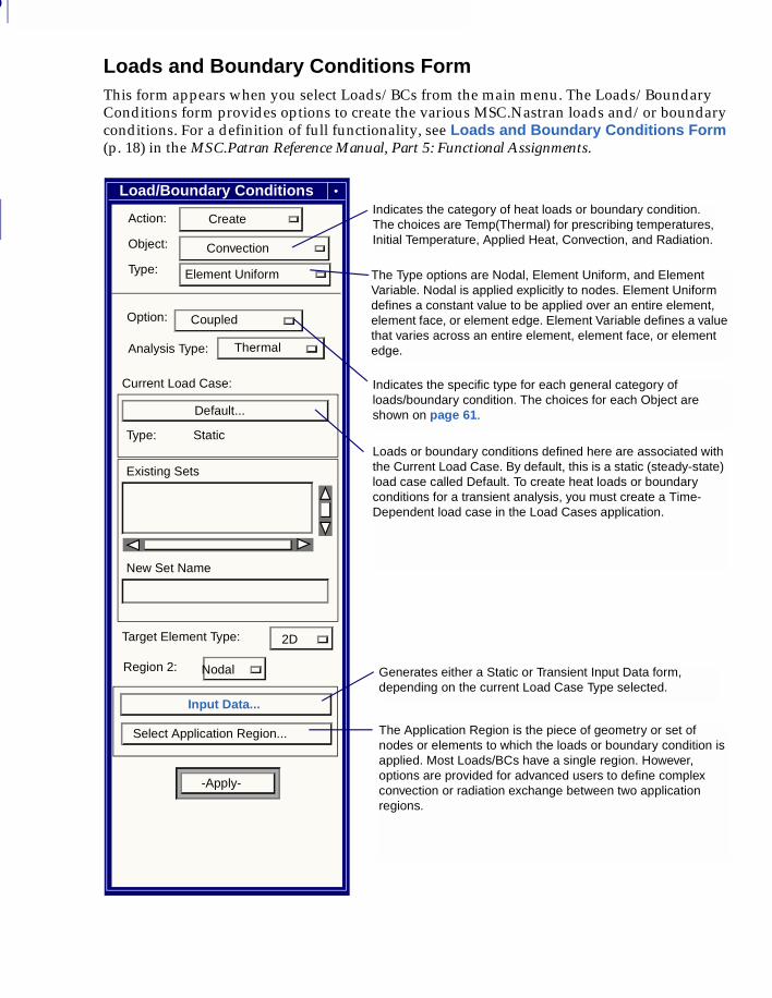
3
60
Loads and Boundary Conditions FormThis form appears when you select Loads/BCs from the main menu. The Loads/Boundary Conditions form provides options to create the various MSC.Nastran loads and/or boundary conditions. For a definition of full functionality, see Loads and Boundary Conditions Form (p. 18) in the MSC.Patran Reference Manual, Part 5: Functional Assignments.
Indicates the category of heat loads or boundary condition. The choices are Temp(Thermal) for prescribing temperatures, Initial Temperature, Applied Heat, Convection, and Radiation.
The Type options are Nodal, Element Uniform, and Element Variable. Nodal is applied explicitly to nodes. Element Uniform defines a constant value to be applied over an entire element, element face, or element edge. Element Variable defines a value that varies across an entire element, element face, or element edge.
Indicates the specific type for each general category of loads/boundary condition. The choices for each Object are shown on page 61.
Loads or boundary conditions defined here are associated with the Current Load Case. By default, this is a static (steady-state) load case called Default. To create heat loads or boundary conditions for a transient analysis, you must create a Time-Dependent load case in the Load Cases application.
The Application Region is the piece of geometry or set of nodes or elements to which the loads or boundary condition is applied. Most Loads/BCs have a single region. However, options are provided for advanced users to define complex convection or radiation exchange between two application regions.
Generates either a Static or Transient Input Data form, depending on the current Load Case Type selected.
Load/Boundary Conditions
Action: Create
Analysis Type:
Type: Element Uniform
Target Element Type: 2D
Object: Convection
Current Load Case:
Default...
Type: Static
Existing Sets
New Set Name
Select Application Region...
-Apply-
Input Data...
Option: Coupled
Thermal
Region 2: Nodal
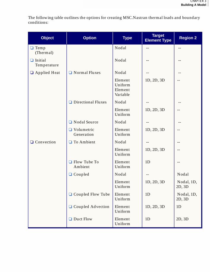
61CHAPTER 3Building A Model
3
The following table outlines the options for creating MSC.Nastran thermal loads and boundary conditions:
Object Option Type Target Element Type Region 2
❏ Temp (Thermal)
Nodal -- --
❏ Initial Temperature
Nodal -- --
❏ Applied Heat ❏ Normal Fluxes Nodal -- --
Element UniformElement Variable
1D, 2D, 3D --
❏ Directional Fluxes Nodal -- --
Element Uniform
1D, 2D, 3D --
❏ Nodal Source Nodal -- --
❏ Volumetric Generation
Element Uniform
1D, 2D, 3D --
❏ Convection ❏ To Ambient Nodal -- --
Element Uniform
1D, 2D, 3D --
❏ Flow Tube To Ambient
Element Uniform
1D --
❏ Coupled Nodal -- Nodal
Element Uniform
1D, 2D, 3D Nodal, 1D, 2D, 3D
❏ Coupled Flow Tube Element Uniform
1D Nodal, 1D, 2D, 3D
❏ Coupled Advection Element Uniform
1D, 2D, 3D 1D
❏ Duct Flow Element Uniform
1D 2D, 3D
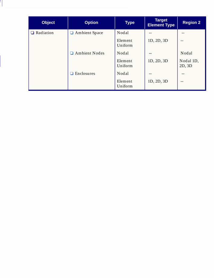
3
62
❏ Radiation ❏ Ambient Space Nodal -- --
Element Uniform
1D, 2D, 3D --
❏ Ambient Nodes Nodal -- Nodal
Element Uniform
1D, 2D, 3D Nodal 1D, 2D, 3D
❏ Enclosures Nodal -- --
Element Uniform
1D, 2D, 3D --
Object Option Type Target Element Type Region 2

63CHAPTER 3Building A Model
3
Input Data Forms--Basic and Advanced Options
Many of the input data forms have a Basic format and an Advanced format. The default is the Basic format, but you can change the format to Advanced using the option menu at the top of the form.
Many of the advanced forms contain a databox called Control Node ID. If an existing node is selected in this databox, the temperature at this node during the analysis is used as an implicit load multiplier, depending on the exact application.
Another advanced option is the Film Node ID that appears on forms for defining convection boundary conditions. This option allows an existing node to be selected. The temperature of this node during the analysis is used to define the temperature of the fluid used in determining the temperature-dependent fluid material properties involved in the calculation of the convection heat transfer coefficient.
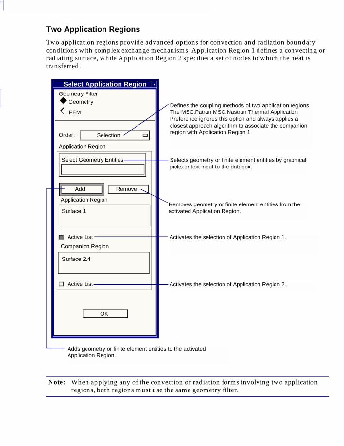
3
64
Two Application Regions
Two application regions provide advanced options for convection and radiation boundary conditions with complex exchange mechanisms. Application Region 1 defines a convecting or radiating surface, while Application Region 2 specifies a set of nodes to which the heat is transferred.
Note: When applying any of the convection or radiation forms involving two application regions, both regions must use the same geometry filter.
Select Application RegionGeometry Filter
Geometry
FEM
Order: Selection
Application Region
Select Geometry Entities
Add Remove
Application Region
Active List
Companion Region
Active List
OK
Defines the coupling methods of two application regions. The MSC.Patran MSC.Nastran Thermal Application Preference ignores this option and always applies a closest approach algorithm to associate the companion region with Application Region 1.
Selects geometry or finite element entities by graphical picks or text input to the databox.
Activates the selection of Application Region 1.
Activates the selection of Application Region 2.
Surface 1
Surface 2.4
Adds geometry or finite element entities to the activated Application Region.
Removes geometry or finite element entities from the activated Application Region.
◆
◆◆
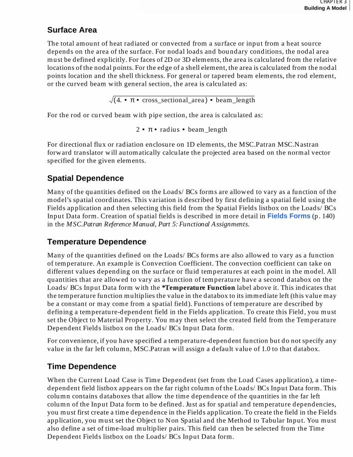
65CHAPTER 3Building A Model
3
Surface Area
The total amount of heat radiated or convected from a surface or input from a heat source depends on the area of the surface. For nodal loads and boundary conditions, the nodal area must be defined explicitly. For faces of 2D or 3D elements, the area is calculated from the relative locations of the nodal points. For the edge of a shell element, the area is calculated from the nodal points location and the shell thickness. For general or tapered beam elements, the rod element, or the curved beam with general section, the area is calculated as:
For the rod or curved beam with pipe section, the area is calculated as:
For directional flux or radiation enclosure on 1D elements, the MSC.Patran MSC.Nastran forward translator will automatically calculate the projected area based on the normal vector specified for the given elements.
Spatial Dependence
Many of the quantities defined on the Loads/BCs forms are allowed to vary as a function of the model’s spatial coordinates. This variation is described by first defining a spatial field using the Fields application and then selecting this field from the Spatial Fields listbox on the Loads/BCs Input Data form. Creation of spatial fields is described in more detail in Fields Forms (p. 140) in the MSC.Patran Reference Manual, Part 5: Functional Assignments.
Temperature Dependence
Many of the quantities defined on the Loads/BCs forms are also allowed to vary as a function of temperature. An example is Convection Coefficient. The convection coefficient can take on different values depending on the surface or fluid temperatures at each point in the model. All quantities that are allowed to vary as a function of temperature have a second databox on the Loads/BCs Input Data form with the *Temperature Function label above it. This indicates that the temperature function multiplies the value in the databox to its immediate left (this value may be a constant or may come from a spatial field). Functions of temperature are described by defining a temperature-dependent field in the Fields application. To create this Field, you must set the Object to Material Property. You may then select the created field from the Temperature Dependent Fields listbox on the Loads/BCs Input Data form.
For convenience, if you have specified a temperature-dependent function but do not specify any value in the far left column, MSC.Patran will assign a default value of 1.0 to that databox.
Time Dependence
When the Current Load Case is Time Dependent (set from the Load Cases application), a time-dependent field listbox appears on the far right column of the Loads/BCs Input Data form. This column contains databoxes that allow the time dependence of the quantities in the far left column of the Input Data form to be defined. Just as for spatial and temperature dependencies, you must first create a time dependence in the Fields application. To create the field in the Fields application, you must set the Object to Non Spatial and the Method to Tabular Input. You must also define a set of time-load multiplier pairs. This field can then be selected from the Time Dependent Fields listbox on the Loads/BCs Input Data form.
4. π• cross_sectional_area•( ) beam_length•
2 π• radius• beam_length•
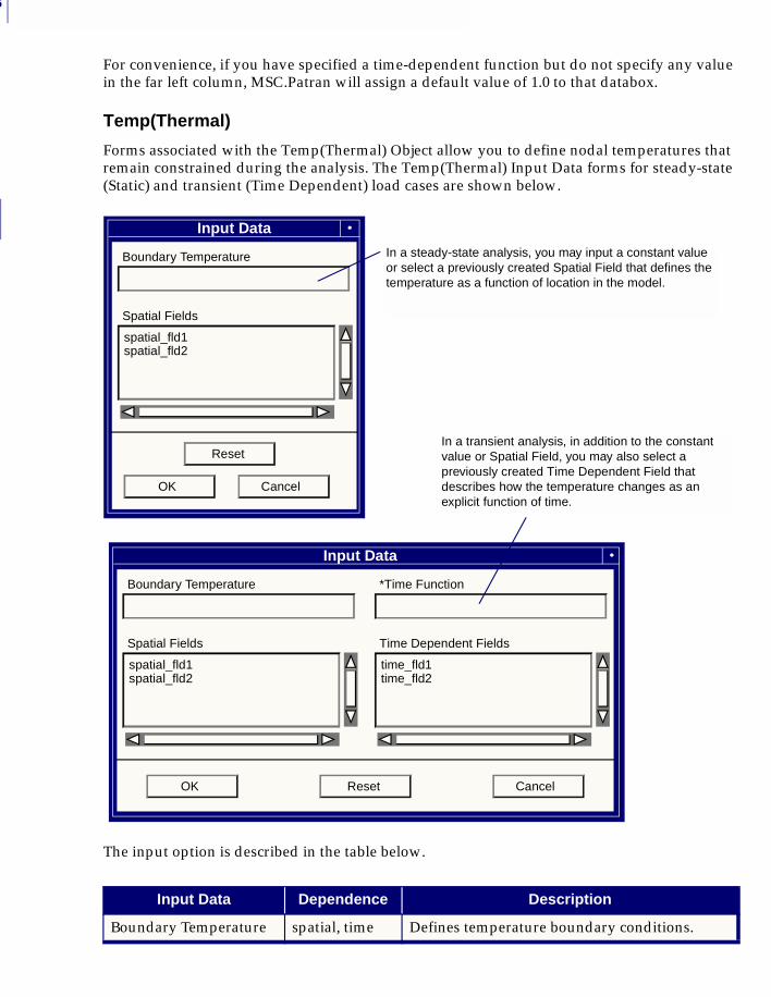
3
66
For convenience, if you have specified a time-dependent function but do not specify any value in the far left column, MSC.Patran will assign a default value of 1.0 to that databox.
Temp(Thermal)
Forms associated with the Temp(Thermal) Object allow you to define nodal temperatures that remain constrained during the analysis. The Temp(Thermal) Input Data forms for steady-state (Static) and transient (Time Dependent) load cases are shown below.
The input option is described in the table below.
Input Data Dependence Description
Boundary Temperature spatial, time Defines temperature boundary conditions.
In a steady-state analysis, you may input a constant value or select a previously created Spatial Field that defines the temperature as a function of location in the model.
In a transient analysis, in addition to the constant value or Spatial Field, you may also select a previously created Time Dependent Field that describes how the temperature changes as an explicit function of time.
Input Data
Boundary Temperature
Spatial Fields
OK Cancel
spatial_fld1spatial_fld2
Reset
Input Data
Boundary Temperature
Spatial Fields
OK Cancel
spatial_fld1spatial_fld2
Reset
*Time Function
Time Dependent Fields
time_fld1time_fld2
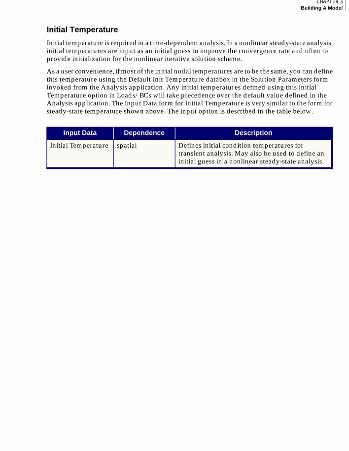
67CHAPTER 3Building A Model
3
Initial Temperature
Initial temperature is required in a time-dependent analysis. In a nonlinear steady-state analysis, initial temperatures are input as an initial guess to improve the convergence rate and often to provide initialization for the nonlinear iterative solution scheme.
As a user convenience, if most of the initial nodal temperatures are to be the same, you can define this temperature using the Default Init Temperature databox in the Solution Parameters form invoked from the Analysis application. Any initial temperatures defined using this Initial Temperature option in Loads/BCs will take precedence over the default value defined in the Analysis application. The Input Data form for Initial Temperature is very similar to the form for steady-state temperature shown above. The input option is described in the table below.
Input Data Dependence Description
Initial Temperature spatial Defines initial condition temperatures for transient analysis. May also be used to define an initial guess in a nonlinear steady-state analysis.
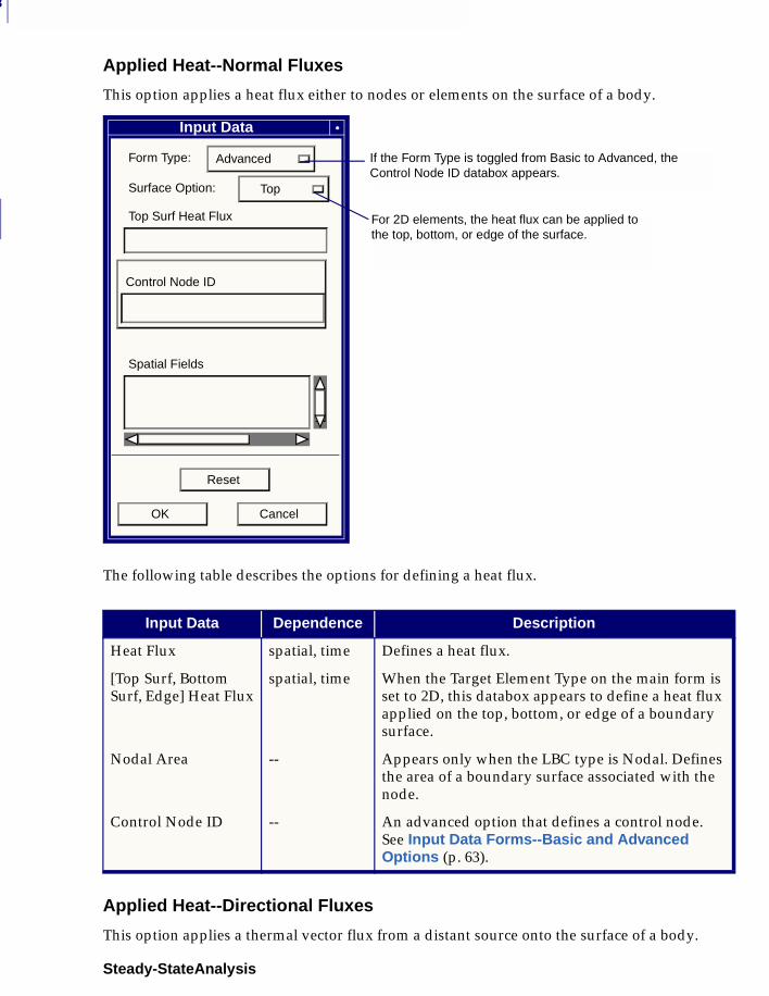
3
68
Applied Heat--Normal Fluxes
This option applies a heat flux either to nodes or elements on the surface of a body.
The following table describes the options for defining a heat flux.
Applied Heat--Directional Fluxes
This option applies a thermal vector flux from a distant source onto the surface of a body.
Steady-StateAnalysis
Input Data Dependence Description
Heat Flux spatial, time Defines a heat flux.
[Top Surf, Bottom Surf, Edge] Heat Flux
spatial, time When the Target Element Type on the main form is set to 2D, this databox appears to define a heat flux applied on the top, bottom, or edge of a boundary surface.
Nodal Area -- Appears only when the LBC type is Nodal. Defines the area of a boundary surface associated with the node.
Control Node ID -- An advanced option that defines a control node. See Input Data Forms--Basic and Advanced Options (p. 63).
Form Type: Advanced
Control Node ID
Surface Option: Top
Top Surf Heat Flux
Spatial Fields
Reset
OK Cancel
If the Form Type is toggled from Basic to Advanced, the Control Node ID databox appears.
For 2D elements, the heat flux can be applied to the top, bottom, or edge of the surface.
Input Data
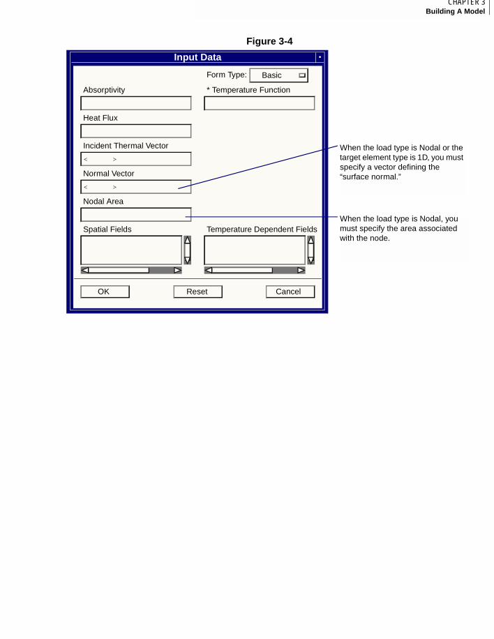
69CHAPTER 3Building A Model
3
Figure 3-4
Input Data
Form Type: Basic
Absorptivity * Temperature Function
Heat Flux
Incident Thermal Vector
< >
Normal Vector
< >
Nodal Area
Spatial Fields Temperature Dependent Fields
ResetOK Cancel
When the load type is Nodal or the target element type is 1D, you must specify a vector defining the “surface normal.”
When the load type is Nodal, you must specify the area associated with the node.
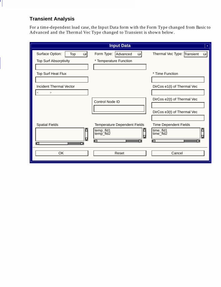
3
70
Transient Analysis
For a time-dependent load case, the Input Data form with the Form Type changed from Basic to Advanced and the Thermal Vec Type changed to Transient is shown below.
Input Data
Form Type: Advanced Thermal Vec Type: Transient
Top Surf Heat Flux * Time Function
Incident Thermal Vector
< >
Surface Option: Top
Top Surf Absorptivity * Temperature Function
DirCos e1(t) of Thermal Vec
DirCos e2(t) of Thermal Vec
DirCos e3(t) of Thermal Vec
Spatial Fields Time Dependent Fields
time_fld1time_fld2
Temperature Dependent Fields
temp_fld1temp_fld2
ResetOK Cancel
Control Node ID
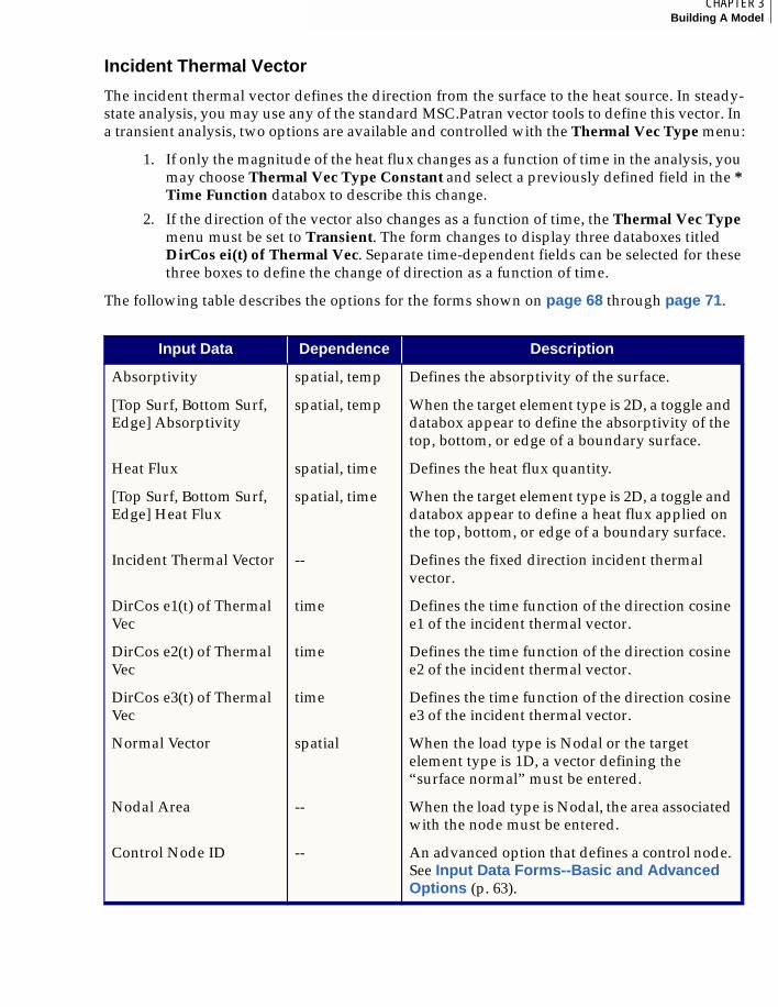
71CHAPTER 3Building A Model
3
Incident Thermal Vector
The incident thermal vector defines the direction from the surface to the heat source. In steady-state analysis, you may use any of the standard MSC.Patran vector tools to define this vector. In a transient analysis, two options are available and controlled with the Thermal Vec Type menu:
1. If only the magnitude of the heat flux changes as a function of time in the analysis, you may choose Thermal Vec Type Constant and select a previously defined field in the * Time Function databox to describe this change.
2. If the direction of the vector also changes as a function of time, the Thermal Vec Type menu must be set to Transient. The form changes to display three databoxes titled DirCos ei(t) of Thermal Vec. Separate time-dependent fields can be selected for these three boxes to define the change of direction as a function of time.
The following table describes the options for the forms shown on page 68 through page 71.
Input Data Dependence Description
Absorptivity spatial, temp Defines the absorptivity of the surface.
[Top Surf, Bottom Surf, Edge] Absorptivity
spatial, temp When the target element type is 2D, a toggle and databox appear to define the absorptivity of the top, bottom, or edge of a boundary surface.
Heat Flux spatial, time Defines the heat flux quantity.
[Top Surf, Bottom Surf, Edge] Heat Flux
spatial, time When the target element type is 2D, a toggle and databox appear to define a heat flux applied on the top, bottom, or edge of a boundary surface.
Incident Thermal Vector -- Defines the fixed direction incident thermal vector.
DirCos e1(t) of Thermal Vec
time Defines the time function of the direction cosine e1 of the incident thermal vector.
DirCos e2(t) of Thermal Vec
time Defines the time function of the direction cosine e2 of the incident thermal vector.
DirCos e3(t) of Thermal Vec
time Defines the time function of the direction cosine e3 of the incident thermal vector.
Normal Vector spatial When the load type is Nodal or the target element type is 1D, a vector defining the “surface normal” must be entered.
Nodal Area -- When the load type is Nodal, the area associated with the node must be entered.
Control Node ID -- An advanced option that defines a control node. See Input Data Forms--Basic and Advanced Options (p. 63).
3
72
Applied Heat--Nodal Source
This option applies a heat flow directly to one or more nodes in the model.
Applied Heat--Volumetric Generation
This option defines a rate of heat generation within the volume of a conduction solid. This heat generation rate can be made a function of temperature by assigning a temperature field to the Heat Generation Multiplier option of the material associated with this solid.
Input Data Dependence Description
Nodal Source spatial, time Defines the heat applied to the nodes.
Input Data Dependence Description
Volumetric Heat Generation
spatial, time Defines the volumetric heat generation in conduction elements.
Control Node ID -- An advanced option that defines a control node. See Input Data Forms--Basic and Advanced Options (p. 63).
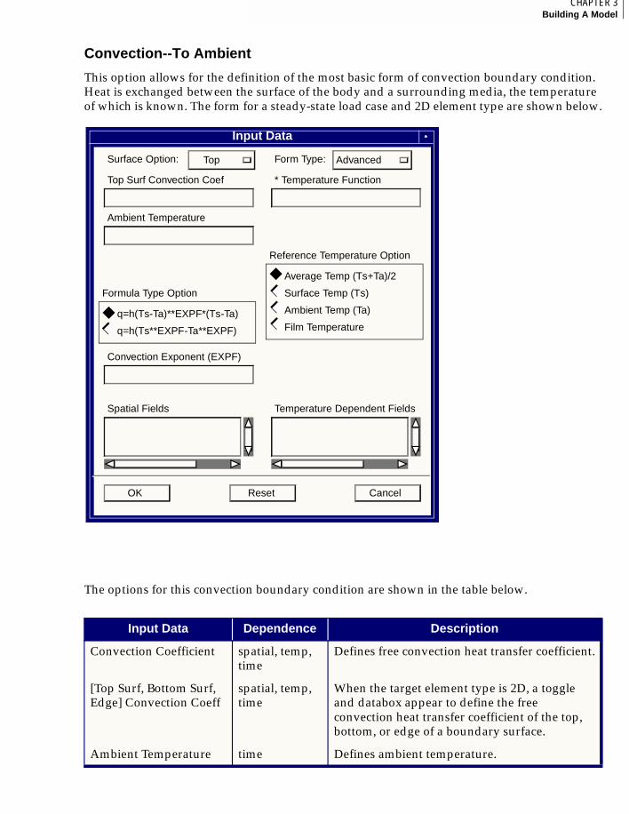
73CHAPTER 3Building A Model
3
Convection--To Ambient
This option allows for the definition of the most basic form of convection boundary condition. Heat is exchanged between the surface of the body and a surrounding media, the temperature of which is known. The form for a steady-state load case and 2D element type are shown below.
The options for this convection boundary condition are shown in the table below.
Input Data Dependence Description
Convection Coefficient spatial, temp, time
Defines free convection heat transfer coefficient.
[Top Surf, Bottom Surf, Edge] Convection Coeff
spatial, temp, time
When the target element type is 2D, a toggle and databox appear to define the free convection heat transfer coefficient of the top, bottom, or edge of a boundary surface.
Ambient Temperature time Defines ambient temperature.
Input Data
Surface Option: Top Form Type: Advanced
Top Surf Convection Coef * Temperature Function
Ambient Temperature
Formula Type Option
q=h(Ts-Ta)**EXPF*(Ts-Ta)
q=h(Ts**EXPF-Ta**EXPF)
Convection Exponent (EXPF)
Reference Temperature Option
Average Temp (Ts+Ta)/2
Surface Temp (Ts)
Ambient Temp (Ta)
Film Temperature
Spatial Fields Temperature Dependent Fields
ResetOK Cancel
◆
◆◆
◆
◆◆
◆◆
◆◆
3
74
With MSC.Nastran Version 68, the MSC.Patran MSC.Nastran Forward Translator will average the values for Surface Temp (Ts) and Ambient Temp (Ta) to acquire the Average Temp (Ts+Ta)/2. Average Temp will be used as the temperature at which the temperature dependent heat transfer coefficient will be determined.
Nodal Area -- When the LBC type is Nodal, this databox appears to define the area of the boundary surface.
Formula Type Option -- An advanced option for defining a customized form of the free convection formula: q = h (Ts-Ta)(expf+1) or q = h (Tsexpf - Taexpf)By default, the first form is chosen with EXPF equal 0.0.
Convection Exponent -- An advanced option for defining EXPF in the above equation.
Reference Temperature Option
-- An advanced option for defining the temperature used in calculating the convection coefficient. The options are: average of surface and ambient temperatures, surface temperature, ambient temperature, or temperature at a user-defined node. By default, this reference temperature is taken as the average of surface and ambient temperatures.
Film Node ID -- An advanced option for selecting an existing node for fluid film temperature.
Input Data Dependence Description
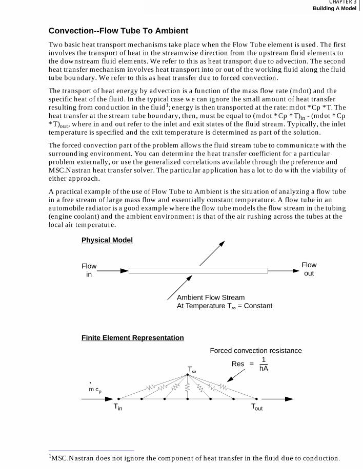
75CHAPTER 3Building A Model
3
Convection--Flow Tube To Ambient
Two basic heat transport mechanisms take place when the Flow Tube element is used. The first involves the transport of heat in the streamwise direction from the upstream fluid elements to the downstream fluid elements. We refer to this as heat transport due to advection. The second heat transfer mechanism involves heat transport into or out of the working fluid along the fluid tube boundary. We refer to this as heat transfer due to forced convection.
The transport of heat energy by advection is a function of the mass flow rate (mdot) and the specific heat of the fluid. In the typical case we can ignore the small amount of heat transfer resulting from conduction in the fluid1; energy is then transported at the rate: mdot * Cp * T. The heat transfer at the stream tube boundary, then, must be equal to (mdot * Cp * T)in - (mdot * Cp * T)out, where in and out refer to the inlet and exit states of the fluid stream. Typically, the inlet temperature is specified and the exit temperature is determined as part of the solution.
The forced convection part of the problem allows the fluid stream tube to communicate with the surrounding environment. You can determine the heat transfer coefficient for a particular problem externally, or use the generalized correlations available through the preference and MSC.Nastran heat transfer solver. The particular application has a lot to do with the viability of either approach.
A practical example of the use of Flow Tube to Ambient is the situation of analyzing a flow tube in a free stream of large mass flow and essentially constant temperature. A flow tube in an automobile radiator is a good example where the flow tube models the flow stream in the tubing (engine coolant) and the ambient environment is that of the air rushing across the tubes at the local air temperature.
1MSC.Nastran does not ignore the component of heat transfer in the fluid due to conduction.
Flowin
Flowout
Ambient Flow StreamAt Temperature T∞ = Constant
Physical Model
Finite Element Representation
T∞
ToutTin
Res1
hA-------=
Forced convection resistance
m cp
.
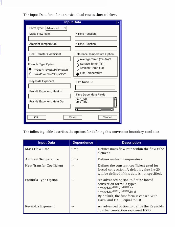
3
76
The Input Data form for a transient load case is shown below.
The following table describes the options for defining this convection boundary condition.
Input Data Dependence Description
Mass Flow Rate time Defines mass flow rate within the flow tube element.
Ambient Temperature time Defines ambient temperature.
Heat Transfer Coefficient -- Defines the constant coefficient used for forced convection. A default value 1.e-20 will be defined if this data is not specified.
Formula Type Option -- An advanced option to define forced convection formula type:h=coef*Reexpr
*Prexpp orh=coef*Reexpr
*Prexpp*k/d
By default, the first form is chosen with EXPR and EXPP equal to 0.0.
Reynolds Exponent -- An advanced option to define the Reynolds number convection exponent EXPR.
Input Data
Form Type: Advanced
Mass Flow Rate * Time Function
Ambient Temperature * Time Function
Heat Transfer Coefficient
Formula Type Option
h=coef*Re**Expr*Pr**Expp
h=k/d*coef*Re**Expr*Pr**
Reynolds Exponent
Prandtl Exponent, Heat In
Prandtl Exponent, Heat Out
Reference Temperature Option
Average Temp (Ts+Ta)/2
Surface Temp (Ts)
Ambient Temp (Ta)
Film Temperature
Time Dependent Fields
time_fld1time_fld2
ResetOK Cancel
Film Node ID
◆
◆◆
◆◆
◆◆
◆
◆◆
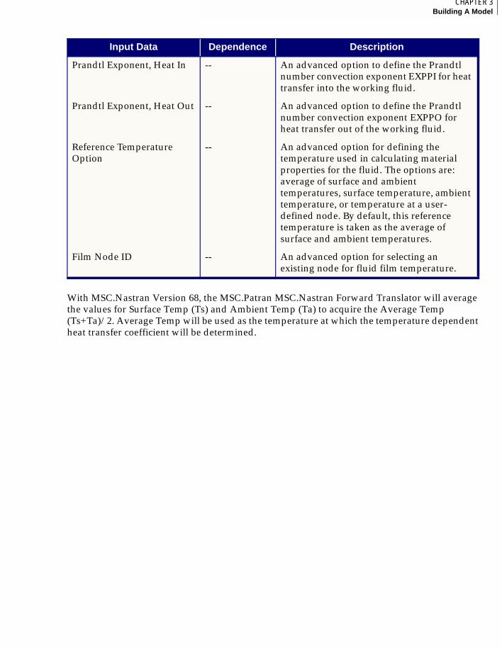
77CHAPTER 3Building A Model
3
With MSC.Nastran Version 68, the MSC.Patran MSC.Nastran Forward Translator will average the values for Surface Temp (Ts) and Ambient Temp (Ta) to acquire the Average Temp (Ts+Ta)/2. Average Temp will be used as the temperature at which the temperature dependent heat transfer coefficient will be determined.
Prandtl Exponent, Heat In -- An advanced option to define the Prandtl number convection exponent EXPPI for heat transfer into the working fluid.
Prandtl Exponent, Heat Out -- An advanced option to define the Prandtl number convection exponent EXPPO for heat transfer out of the working fluid.
Reference Temperature Option
-- An advanced option for defining the temperature used in calculating material properties for the fluid. The options are: average of surface and ambient temperatures, surface temperature, ambient temperature, or temperature at a user-defined node. By default, this reference temperature is taken as the average of surface and ambient temperatures.
Film Node ID -- An advanced option for selecting an existing node for fluid film temperature.
Input Data Dependence Description
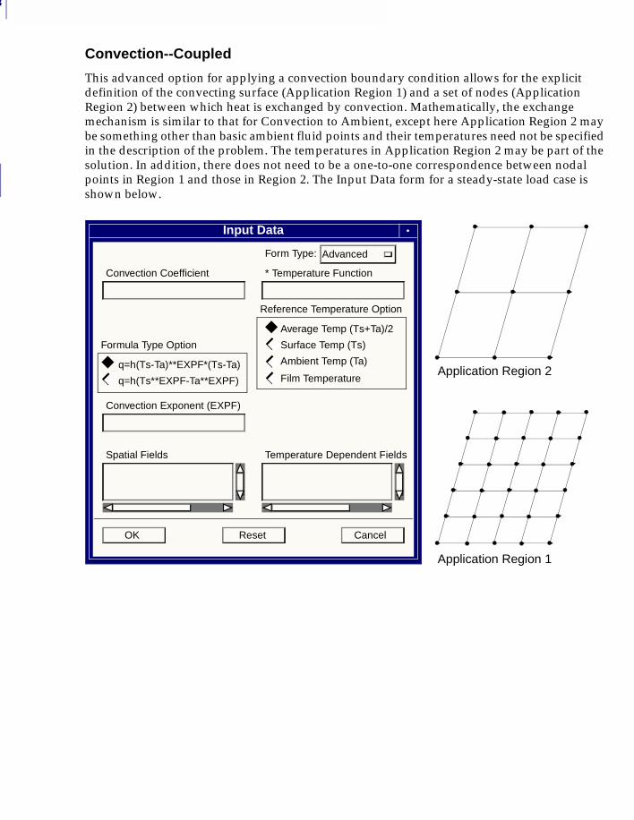
3
78
Convection--Coupled
This advanced option for applying a convection boundary condition allows for the explicit definition of the convecting surface (Application Region 1) and a set of nodes (Application Region 2) between which heat is exchanged by convection. Mathematically, the exchange mechanism is similar to that for Convection to Ambient, except here Application Region 2 may be something other than basic ambient fluid points and their temperatures need not be specified in the description of the problem. The temperatures in Application Region 2 may be part of the solution. In addition, there does not need to be a one-to-one correspondence between nodal points in Region 1 and those in Region 2. The Input Data form for a steady-state load case is shown below.
Input Data
Form Type: Advanced
Convection Coefficient * Temperature Function
Formula Type Option
q=h(Ts-Ta)**EXPF*(Ts-Ta)
q=h(Ts**EXPF-Ta**EXPF)
Convection Exponent (EXPF)
Reference Temperature Option
Average Temp (Ts+Ta)/2
Surface Temp (Ts)
Ambient Temp (Ta)
Film Temperature
Spatial Fields Temperature Dependent Fields
ResetOK Cancel
Application Region 2
Application Region 1
◆
◆◆
◆
◆◆
◆◆
◆◆
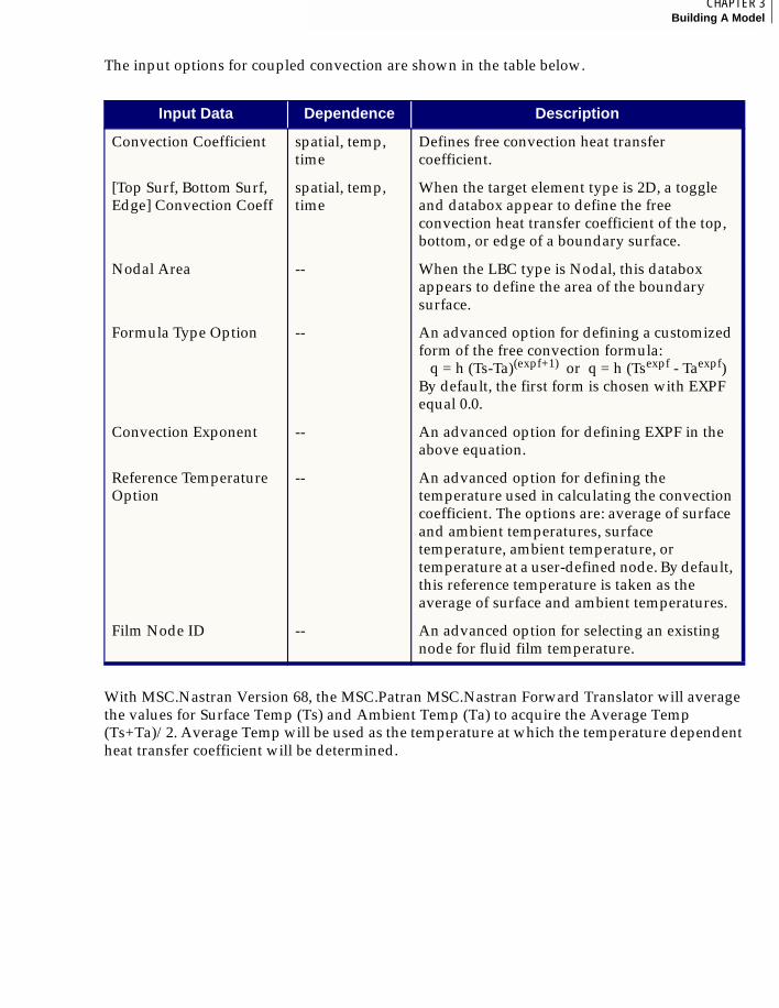
79CHAPTER 3Building A Model
3
The input options for coupled convection are shown in the table below.
With MSC.Nastran Version 68, the MSC.Patran MSC.Nastran Forward Translator will average the values for Surface Temp (Ts) and Ambient Temp (Ta) to acquire the Average Temp (Ts+Ta)/2. Average Temp will be used as the temperature at which the temperature dependent heat transfer coefficient will be determined.
Input Data Dependence Description
Convection Coefficient spatial, temp, time
Defines free convection heat transfer coefficient.
[Top Surf, Bottom Surf, Edge] Convection Coeff
spatial, temp, time
When the target element type is 2D, a toggle and databox appear to define the free convection heat transfer coefficient of the top, bottom, or edge of a boundary surface.
Nodal Area -- When the LBC type is Nodal, this databox appears to define the area of the boundary surface.
Formula Type Option -- An advanced option for defining a customized form of the free convection formula: q = h (Ts-Ta)(expf+1) or q = h (Tsexpf - Taexpf)By default, the first form is chosen with EXPF equal 0.0.
Convection Exponent -- An advanced option for defining EXPF in the above equation.
Reference Temperature Option
-- An advanced option for defining the temperature used in calculating the convection coefficient. The options are: average of surface and ambient temperatures, surface temperature, ambient temperature, or temperature at a user-defined node. By default, this reference temperature is taken as the average of surface and ambient temperatures.
Film Node ID -- An advanced option for selecting an existing node for fluid film temperature.
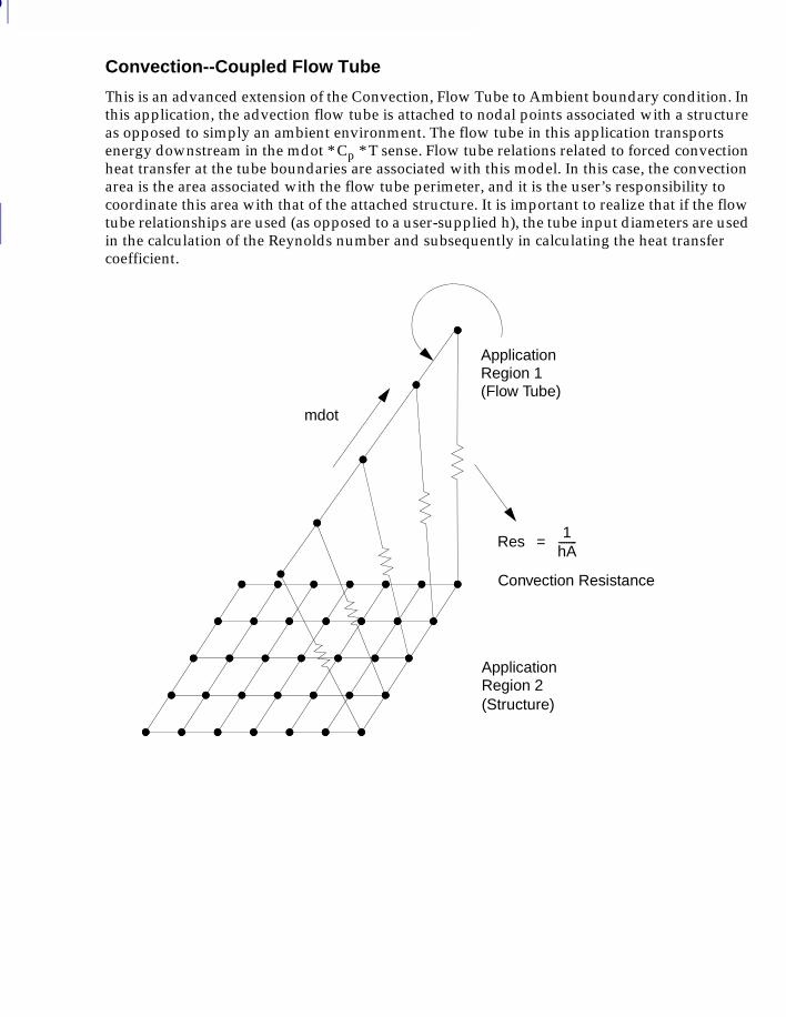
3
80
Convection--Coupled Flow Tube
This is an advanced extension of the Convection, Flow Tube to Ambient boundary condition. In this application, the advection flow tube is attached to nodal points associated with a structure as opposed to simply an ambient environment. The flow tube in this application transports energy downstream in the mdot * Cp * T sense. Flow tube relations related to forced convection heat transfer at the tube boundaries are associated with this model. In this case, the convection area is the area associated with the flow tube perimeter, and it is the user’s responsibility to coordinate this area with that of the attached structure. It is important to realize that if the flow tube relationships are used (as opposed to a user-supplied h), the tube input diameters are used in the calculation of the Reynolds number and subsequently in calculating the heat transfer coefficient.
ApplicationRegion 1(Flow Tube)
Res1
hA-------=
ApplicationRegion 2
mdot
Convection Resistance
(Structure)
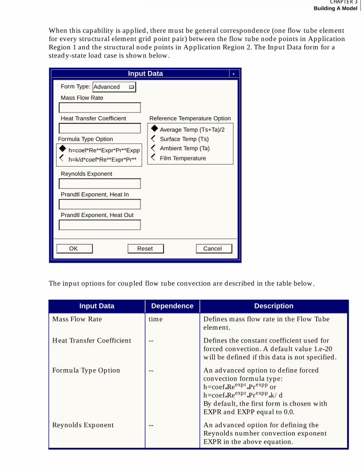
81CHAPTER 3Building A Model
3
When this capability is applied, there must be general correspondence (one flow tube element for every structural element grid point pair) between the flow tube node points in Application Region 1 and the structural node points in Application Region 2. The Input Data form for a steady-state load case is shown below.
The input options for coupled flow tube convection are described in the table below.
Input Data Dependence Description
Mass Flow Rate time Defines mass flow rate in the Flow Tube element.
Heat Transfer Coefficient -- Defines the constant coefficient used for forced convection. A default value 1.e-20 will be defined if this data is not specified.
Formula Type Option -- An advanced option to define forced convection formula type: h=coef*Reexpr
*Prexpp or h=coef*Reexpr
*Prexpp*k/d
By default, the first form is chosen with EXPR and EXPP equal to 0.0.
Reynolds Exponent -- An advanced option for defining the Reynolds number convection exponent EXPR in the above equation.
Input Data
Form Type: Advanced
Mass Flow Rate
Heat Transfer Coefficient
Formula Type Option
h=coef*Re**Expr*Pr**Expp
h=k/d*coef*Re**Expr*Pr**
Reynolds Exponent
Prandtl Exponent, Heat In
Prandtl Exponent, Heat Out
Reference Temperature Option
Average Temp (Ts+Ta)/2
Surface Temp (Ts)
Ambient Temp (Ta)
Film Temperature
ResetOK Cancel
◆◆
◆◆◆◆◆◆
◆
◆
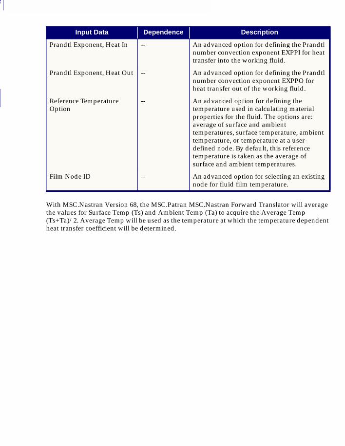
3
82
With MSC.Nastran Version 68, the MSC.Patran MSC.Nastran Forward Translator will average the values for Surface Temp (Ts) and Ambient Temp (Ta) to acquire the Average Temp (Ts+Ta)/2. Average Temp will be used as the temperature at which the temperature dependent heat transfer coefficient will be determined.
Prandtl Exponent, Heat In -- An advanced option for defining the Prandtl number convection exponent EXPPI for heat transfer into the working fluid.
Prandtl Exponent, Heat Out -- An advanced option for defining the Prandtl number convection exponent EXPPO for heat transfer out of the working fluid.
Reference Temperature Option
-- An advanced option for defining the temperature used in calculating material properties for the fluid. The options are: average of surface and ambient temperatures, surface temperature, ambient temperature, or temperature at a user-defined node. By default, this reference temperature is taken as the average of surface and ambient temperatures.
Film Node ID -- An advanced option for selecting an existing node for fluid film temperature.
Input Data Dependence Description
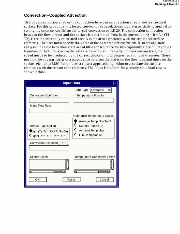
83CHAPTER 3Building A Model
3
Convection--Coupled Advection
This advanced option enables the connection between an advection stream and a structural surface. For this capability, the forced convection tube relationships are essentially turned off by setting the constant coefficient for forced convection to 1.E-20. The convection connection between the flow stream and the surface is determined from basic convection; Q = h * A * (T1 - T2). Here the internally calculated area A is the area associated with the structural surface elements. The user must specify the value of the heat transfer coefficient, h. In steady-state analysis, the flow tube diameters are of little consequence for this capability since no Reynolds Numbers or heat transfer coefficients are determined internally. In transient analysis, the fluid speed needs to be produced by the correct choice of fluid properties and tube diameter. There need not be any particular correspondence between the nodes on the flow tube and those on the surface elements; MSC.Patran uses a closest approach algorithm to associate the surface elements with the stream tube elements. The Input Data form for a steady-state load case is shown below.
Input Data
Form Type: Advanced
Convection Coefficient * Temperature Function
Mass Flow Rate
Formula Type Option
q=h(Ts-Ta)**EXPF*(Ts-Ta)
q=h(Ts**EXPF-Ta**EXPF)
Convection Exponent (EXPF)
Reference Temperature Option
Average Temp (Ts+Ta)/2
Surface Temp (Ts)
Ambient Temp (Ta)
Film Temperature
Spatial Fields Temperature Dependent Fields
ResetOK Cancel
◆
◆
◆◆
◆◆
◆◆
◆◆
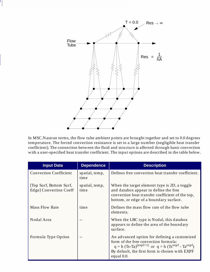
3
84
In MSC.Nastran terms, the flow tube ambient points are brought together and set to 0.0 degrees temperature. The forced convection resistance is set to a large number (negligible heat transfer coefficient). The connection between the fluid and structure is affected through basic convection with a user-specified heat transfer coefficient. The input options are described in the table below.
Input Data Dependence Description
Convection Coefficient spatial, temp, time
Defines free convection heat transfer coefficient.
[Top Surf, Bottom Surf, Edge] Convection Coeff
spatial, temp, time
When the target element type is 2D, a toggle and databox appear to define the free convection heat transfer coefficient of the top, bottom, or edge of a boundary surface.
Mass Flow Rate time Defines the mass flow rate of the flow tube elements.
Nodal Area -- When the LBC type is Nodal, this databox appears to define the area of the boundary surface.
Formula Type Option -- An advanced option for defining a customized form of the free convection formula: q = h (Ts-Ta)(expf+1) or q = h (Tsexpf - Taexpf)By default, the first form is chosen with EXPF equal 0.0.
Flow
Res1
hA-------=
Tube
T = 0.0 Res → ∞
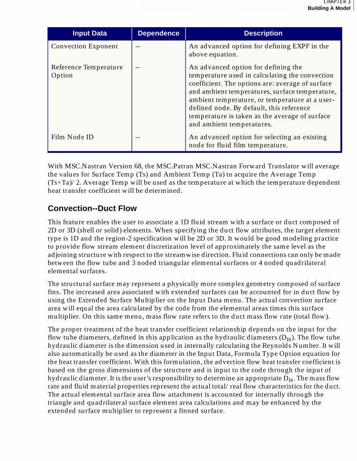
85CHAPTER 3Building A Model
3
With MSC.Nastran Version 68, the MSC.Patran MSC.Nastran Forward Translator will average the values for Surface Temp (Ts) and Ambient Temp (Ta) to acquire the Average Temp (Ts+Ta)/2. Average Temp will be used as the temperature at which the temperature dependent heat transfer coefficient will be determined.
Convection--Duct Flow
This feature enables the user to associate a 1D fluid stream with a surface or duct composed of 2D or 3D (shell or solid) elements. When specifying the duct flow attributes, the target element type is 1D and the region-2 specification will be 2D or 3D. It would be good modeling practice to provide flow stream element discretization level of approximately the same level as the adjoining structure with respect to the streamwise direction. Fluid connections can only be made between the flow tube and 3 noded triangular elemental surfaces or 4 noded quadrilateral elemental surfaces.
The structural surface may represent a physically more complex geometry composed of surface fins. The increased area associated with extended surfaces can be accounted for in duct flow by using the Extended Surface Multiplier on the Input Data menu. The actual convection surface area will equal the area calculated by the code from the elemental areas times this surface multiplier. On this same menu, mass flow rate refers to the duct mass flow rate (total flow).
The proper treatment of the heat transfer coefficient relationship depends on the input for the flow tube diameters, defined in this application as the hydraulic diameters (DH). The flow tube hydraulic diameter is the dimension used in internally calculating the Reynolds Number. It will also automatically be used as the diameter in the Input Data, Formula Type Option equation for the heat transfer coefficient. With this formulation, the advection flow heat transfer coefficient is based on the gross dimensions of the structure and is input to the code through the input of hydraulic diameter. It is the user’s responsibility to determine an appropriate DH. The mass flow rate and fluid material properties represent the actual total/real flow characteristics for the duct. The actual elemental surface area flow attachment is accounted for internally through the triangle and quadrilateral surface element area calculations and may be enhanced by the extended surface multiplier to represent a finned surface.
Convection Exponent -- An advanced option for defining EXPF in the above equation.
Reference Temperature Option
-- An advanced option for defining the temperature used in calculating the convection coefficient. The options are: average of surface and ambient temperatures, surface temperature, ambient temperature, or temperature at a user-defined node. By default, this reference temperature is taken as the average of surface and ambient temperatures.
Film Node ID -- An advanced option for selecting an existing node for fluid film temperature.
Input Data Dependence Description
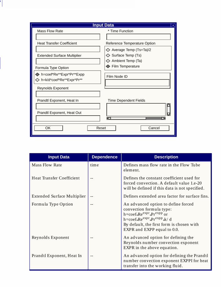
3
86
Input Data Dependence Description
Mass Flow Rate time Defines mass flow rate in the Flow Tube element.
Heat Transfer Coefficient -- Defines the constant coefficient used for forced convection. A default value 1.e-20 will be defined if this data is not specified.
Extended Surface Multiplier -- Defines extended area factor for surface fins.
Formula Type Option -- An advanced option to define forced convection formula type: h=coef*Reexpr
*Prexpp or h=coef*Reexpr
*Prexpp*k/d
By default, the first form is chosen with EXPR and EXPP equal to 0.0.
Reynolds Exponent -- An advanced option for defining the Reynolds number convection exponent EXPR in the above equation.
Prandtl Exponent, Heat In -- An advanced option for defining the Prandtl number convection exponent EXPPI for heat transfer into the working fluid.
Input DataMass Flow Rate * Time Function
Heat Transfer Coefficient
Extended Surface Multiplier
Formula Type Option
h=coef*Re**Expr*Pr**Expp
h=k/d*coef*Re**Expr*Pr**
Reynolds Exponent
Prandtl Exponent, Heat In
Prandtl Exponent, Heat Out
Reference Temperature Option
Average Temp (Ts+Ta)/2
Surface Temp (Ts)
Ambient Temp (Ta)
Film Temperature
Film Node ID
Time Dependent Fields
ResetOK Cancel
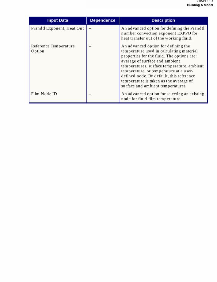
87CHAPTER 3Building A Model
3
Prandtl Exponent, Heat Out -- An advanced option for defining the Prandtl number convection exponent EXPPO for heat transfer out of the working fluid.
Reference Temperature Option
-- An advanced option for defining the temperature used in calculating material properties for the fluid. The options are: average of surface and ambient temperatures, surface temperature, ambient temperature, or temperature at a user-defined node. By default, this reference temperature is taken as the average of surface and ambient temperatures.
Film Node ID -- An advanced option for selecting an existing node for fluid film temperature.
Input Data Dependence Description
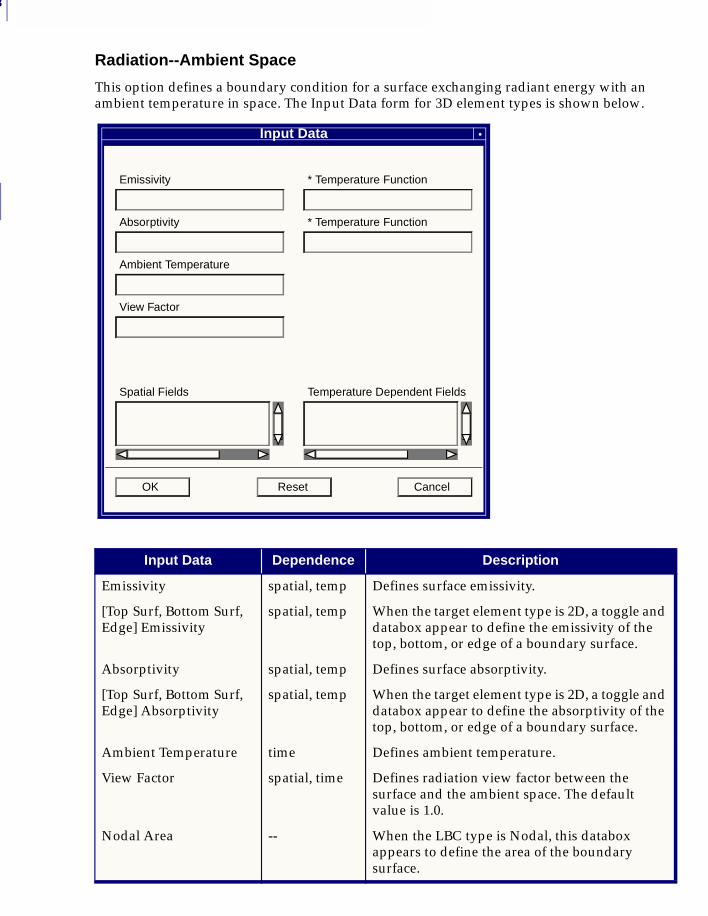
3
88
Radiation--Ambient Space
This option defines a boundary condition for a surface exchanging radiant energy with an ambient temperature in space. The Input Data form for 3D element types is shown below.
Input Data Dependence Description
Emissivity spatial, temp Defines surface emissivity.
[Top Surf, Bottom Surf, Edge] Emissivity
spatial, temp When the target element type is 2D, a toggle and databox appear to define the emissivity of the top, bottom, or edge of a boundary surface.
Absorptivity spatial, temp Defines surface absorptivity.
[Top Surf, Bottom Surf, Edge] Absorptivity
spatial, temp When the target element type is 2D, a toggle and databox appear to define the absorptivity of the top, bottom, or edge of a boundary surface.
Ambient Temperature time Defines ambient temperature.
View Factor spatial, time Defines radiation view factor between the surface and the ambient space. The default value is 1.0.
Nodal Area -- When the LBC type is Nodal, this databox appears to define the area of the boundary surface.
Input Data
Emissivity * Temperature Function
Absorptivity * Temperature Function
Ambient Temperature
View Factor
Spatial Fields Temperature Dependent Fields
ResetOK Cancel
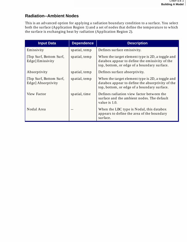
89CHAPTER 3Building A Model
3
Radiation--Ambient Nodes
This is an advanced option for applying a radiation boundary condition to a surface. You select both the surface (Application Region 1) and a set of nodes that define the temperature to which the surface is exchanging heat by radiation (Application Region 2).
Input Data Dependence Description
Emissivity spatial, temp Defines surface emissivity.
[Top Surf, Bottom Surf, Edge] Emissivity
spatial, temp When the target element type is 2D, a toggle and databox appear to define the emissivity of the top, bottom, or edge of a boundary surface.
Absorptivity spatial, temp Defines surface absorptivity.
[Top Surf, Bottom Surf, Edge] Absorptivity
spatial, temp When the target element type is 2D, a toggle and databox appear to define the absorptivity of the top, bottom, or edge of a boundary surface.
View Factor spatial, time Defines radiation view factor between the surface and the ambient nodes. The default value is 1.0.
Nodal Area -- When the LBC type is Nodal, this databox appears to define the area of the boundary surface.
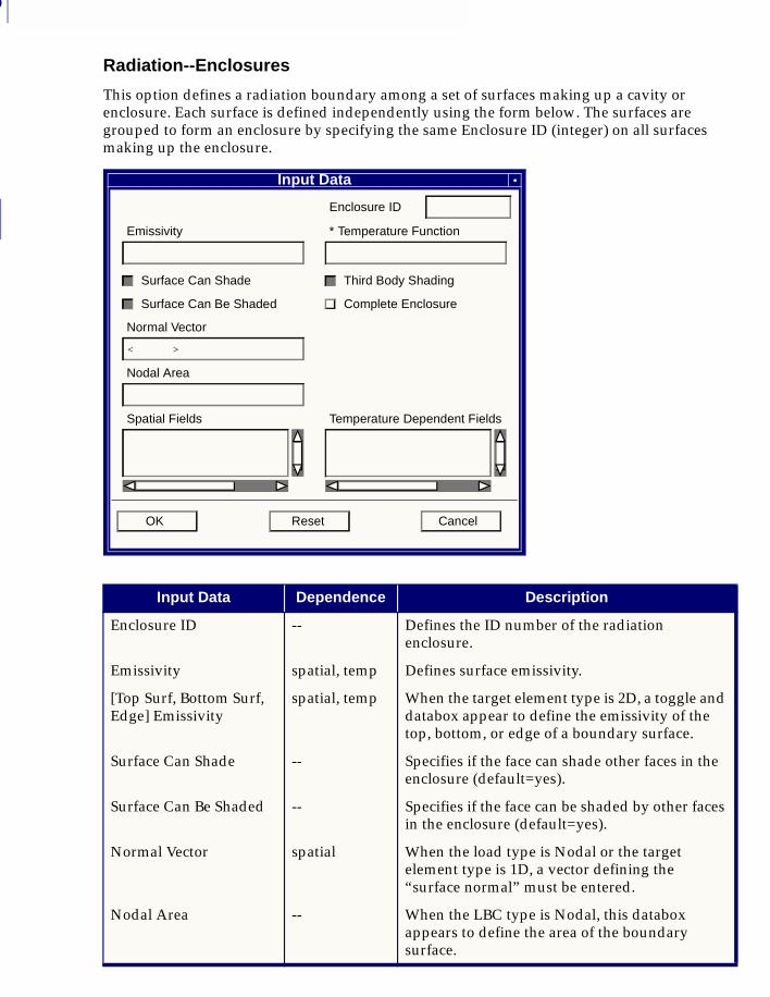
3
90
Radiation--Enclosures
This option defines a radiation boundary among a set of surfaces making up a cavity or enclosure. Each surface is defined independently using the form below. The surfaces are grouped to form an enclosure by specifying the same Enclosure ID (integer) on all surfaces making up the enclosure.
Input Data Dependence Description
Enclosure ID -- Defines the ID number of the radiation enclosure.
Emissivity spatial, temp Defines surface emissivity.
[Top Surf, Bottom Surf, Edge] Emissivity
spatial, temp When the target element type is 2D, a toggle and databox appear to define the emissivity of the top, bottom, or edge of a boundary surface.
Surface Can Shade -- Specifies if the face can shade other faces in the enclosure (default=yes).
Surface Can Be Shaded -- Specifies if the face can be shaded by other faces in the enclosure (default=yes).
Normal Vector spatial When the load type is Nodal or the target element type is 1D, a vector defining the “surface normal” must be entered.
Nodal Area -- When the LBC type is Nodal, this databox appears to define the area of the boundary surface.
Input Data
Enclosure ID
Emissivity * Temperature Function
Surface Can Shade Third Body Shading
Surface Can Be Shaded Complete Enclosure
Normal Vector
< >
Nodal Area
Spatial Fields Temperature Dependent Fields
ResetOK Cancel
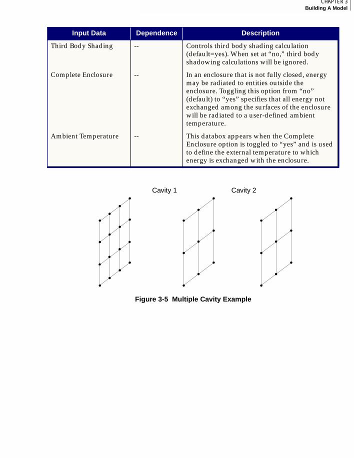
91CHAPTER 3Building A Model
3
Figure 3-5 Multiple Cavity Example
Third Body Shading -- Controls third body shading calculation (default=yes). When set at “no,” third body shadowing calculations will be ignored.
Complete Enclosure -- In an enclosure that is not fully closed, energy may be radiated to entities outside the enclosure. Toggling this option from “no” (default) to “yes” specifies that all energy not exchanged among the surfaces of the enclosure will be radiated to a user-defined ambient temperature.
Ambient Temperature -- This databox appears when the Complete Enclosure option is toggled to “yes” and is used to define the external temperature to which energy is exchanged with the enclosure.
Input Data Dependence Description
Cavity 1 Cavity 2
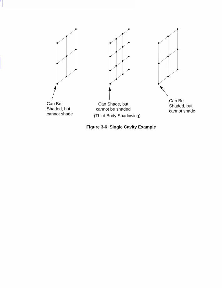
3
92
Figure 3-6 Single Cavity Example
Can BeShaded, but
Can Shade, butCan BeShaded, but
cannot be shadedcannot shade
cannot shade(Third Body Shadowing)
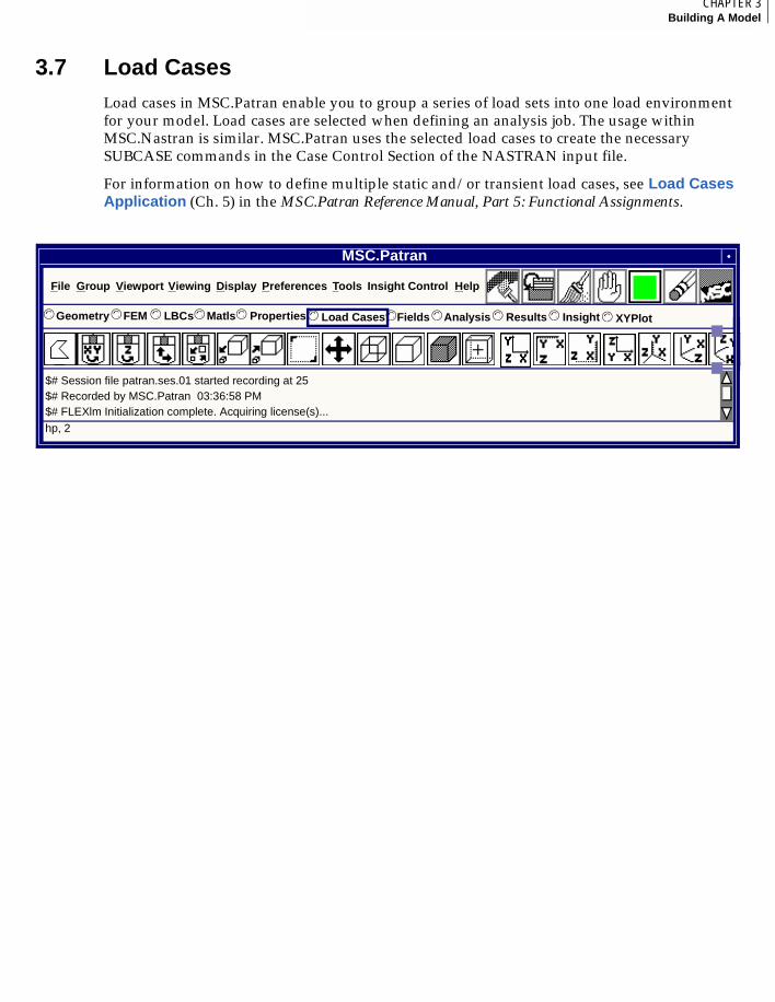
93CHAPTER 3Building A Model
3
3.7 Load CasesLoad cases in MSC.Patran enable you to group a series of load sets into one load environment for your model. Load cases are selected when defining an analysis job. The usage within MSC.Nastran is similar. MSC.Patran uses the selected load cases to create the necessary SUBCASE commands in the Case Control Section of the NASTRAN input file.
For information on how to define multiple static and/or transient load cases, see Load Cases Application (Ch. 5) in the MSC.Patran Reference Manual, Part 5: Functional Assignments.
MSC.Patran
hp, 2
$# Session file patran.ses.01 started recording at 25$# Recorded by MSC.Patran 03:36:58 PM$# FLEXlm Initialization complete. Acquiring license(s)...
File Group Viewport Display Preferences Tools HelpInsight Control
Geometry© FEM LBCs Matls Properties© ©© © Load Cases© Fields Analysis Results Insight© ©© © XYPlot©
Viewing

3
94
MSC.Patran MSC.Nastran Preference Guide, Volume 2: Thermal Analysis
CHAPTER
4 Running a Thermal Analysis
■ Introduction
■ Review of the Analysis Form
■ Translation Parameters
■ Solution Types
■ Direct Text Input
■ Subcase Create
■ Subcase Select
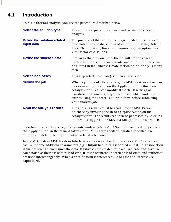
4
96
4.1 IntroductionTo run a thermal analysis, you use the procedure described below.
To submit a single load case, steady-state analysis job to MSC.Nastran, you need only click on the Apply button on the main Analysis form. MSC.Patran will automatically control the appropriate default settings and other related selections.
In the MSC.Patran MSC.Nastran Interface, a subcase can be thought of as a MSC.Patran load case with some additional parameters (e.g., Output Requests) associated with it. This association is further strengthened since the default subcases are created for each load case and have the same name as their associated load case. In this document, the terms “load case” and “subcase” are used interchangeably. When a specific form is referenced, Load case and Subcase are capitalized.
Select the solution type The solution type can be either steady-state or transient analysis.
Define the solution related input data
The purpose of this step is to change the default settings of job-related input data, such as Maximum Run Time, Default Initial Temperature, Radiation Parameters, and options for view factor calculations.
Define the subcase data Similar to the previous step, the defaults for nonlinear iteration controls, time increments, and output requests can be altered in the Subcase Create section of the Analysis menu form.
Select load cases This step selects load case(s) for an analysis job.
Submit the job When a job is ready for analysis, the MSC.Nastran solver can be retrieved by clicking on the Apply button on the main Analysis form. You can modify the default settings of translation parameters, or you can insert additional data entries using the Direct Text Input form before submitting your analysis job.
Read the analysis results The analysis results must be read into the MSC.Patran database by invoking the Read Output2 Action on the Analysis form. The results can then be processed by selecting the Results toggle on the MSC.Patran application selections.
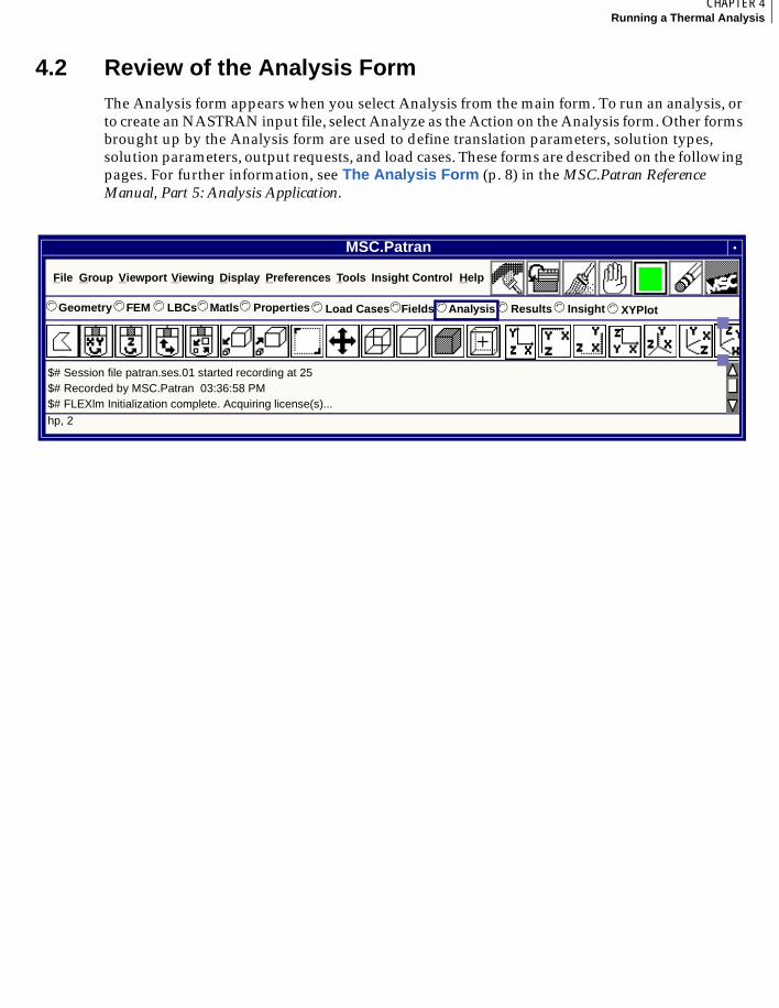
97CHAPTER 4Running a Thermal Analysis
4
4.2 Review of the Analysis FormThe Analysis form appears when you select Analysis from the main form. To run an analysis, or to create an NASTRAN input file, select Analyze as the Action on the Analysis form. Other forms brought up by the Analysis form are used to define translation parameters, solution types, solution parameters, output requests, and load cases. These forms are described on the following pages. For further information, see The Analysis Form (p. 8) in the MSC.Patran Reference Manual, Part 5: Analysis Application.
MSC.Patran
hp, 2
$# Session file patran.ses.01 started recording at 25$# Recorded by MSC.Patran 03:36:58 PM$# FLEXlm Initialization complete. Acquiring license(s)...
File Group Viewport Display Preferences Tools HelpInsight Control
Geometry© FEM LBCs Matls Properties© ©© © Load Cases© Fields Analysis Results Insight© ©© © XYPlot©
Viewing
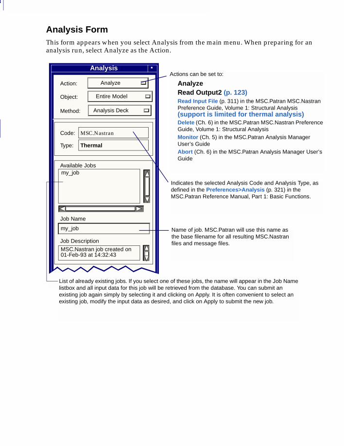
4
98
Analysis FormThis form appears when you select Analysis from the main menu. When preparing for an analysis run, select Analyze as the Action.
Analysis
AnalyzeAction:
Code:
Entire ModelObject:
Analysis DeckMethod:
Job Name
Name of job. MSC.Patran will use this name as the base filename for all resulting MSC.Nastran files and message files.
Indicates the selected Analysis Code and Analysis Type, as defined in the Preferences>Analysis (p. 321) in the MSC.Patran Reference Manual, Part 1: Basic Functions.
Available Jobs
MSC.Nastran
Type: Thermal
my_job
Job Description
MSC.Nastran job created on01-Feb-93 at 14:32:43
Actions can be set to:
AnalyzeRead Output2 (p. 123)Read Input File (p. 311) in the MSC.Patran MSC.Nastran Preference Guide, Volume 1: Structural Analysis (support is limited for thermal analysis)Delete (Ch. 6) in the MSC.Patran MSC.Nastran Preference Guide, Volume 1: Structural Analysis Monitor (Ch. 5) in the MSC.Patran Analysis Manager User’s GuideAbort (Ch. 6) in the MSC.Patran Analysis Manager User’s Guide
my_job
List of already existing jobs. If you select one of these jobs, the name will appear in the Job Name listbox and all input data for this job will be retrieved from the database. You can submit an existing job again simply by selecting it and clicking on Apply. It is often convenient to select an existing job, modify the input data as desired, and click on Apply to submit the new job.
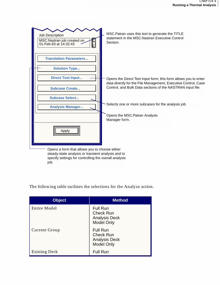
99CHAPTER 4Running a Thermal Analysis
4
The following table outlines the selections for the Analyze action.
Object Method
Entire Model Full RunCheck RunAnalysis DeckModel Only
Current Group Full RunCheck RunAnalysis DeckModel Only
Existing Deck Full Run
Translation Parameters...
Solution Type...
Apply
Job Description
MSC.Nastran job created on01-Feb-93 at 14:32:43
MSC.Patran uses this text to generate the TITLE statement in the MSC.Nastran Executive Control Section.
Subcase Select...
Subcase Create...
Opens the MSC.Patran Analysis Manager form.
Direct Text Input...
Analysis Manager...
Opens the Direct Text Input form; this form allows you to enter data directly for the File Management, Executive Control, Case Control, and Bulk Data sections of the NASTRAN input file.
Opens a form that allows you to choose either steady-state analysis or transient analysis and to specify settings for controlling the overall analysis job.
Selects one or more subcases for the analysis job.
4
100
The Object indicates which part of the model is to be analyzed. There are three choices for thermal analysis: Entire Model, Current Group, and Existing Deck.
The Method indicates how far the translation is to be taken.The methods are as follow:
Entire Model Indicates that the whole model is to be analyzed.
Current Group Indicates that only part of the model is to be analyzed. To do this, you create a group of that part, confirm that it is the current group, then select Current Group as the Object. For more information, see The Group Menu (p. 213) in the MSC.Patran Reference Manual, Part 1: Basic Functions.
Existing Deck Means that you wish simply to submit an existing input file to MSC.Nastran. To form the input filename, MSC.Patran appends the suffix “.bdf” to the jobname appearing in the Job Name listbox. This file must reside in the current directory.
Full Run Is the selected type if an Analysis Deck translation is performed, and the resulting input file is submitted to MSC.Nastran for complete analysis.
Check Run Is the selected type if an Analysis Deck translation is performed, and the resulting input file is submitted to MSC.Nastran for a check run only.
Analysis Deck Is the selected type if the Model Deck translation is performed, plus all load case, analysis type and analysis parameter data are translated. A complete input file, ready for MSC.Nastran, will be generated.
Model Only Is the selected type if a Bulk Data file is created that contains only the model data including node, element, coordinate frame, element property, material property, and loads and boundary conditions data. The translation stops at that point.
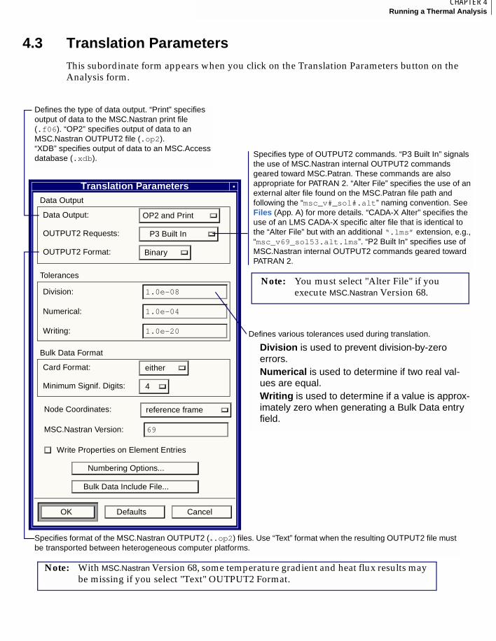
101CHAPTER 4Running a Thermal Analysis
4
4.3 Translation ParametersThis subordinate form appears when you click on the Translation Parameters button on the Analysis form.
Translation ParametersData Output
Data Output: OP2 and Print
OUTPUT2 Requests: P3 Built In
OUTPUT2 Format: Binary
Tolerances
Division: 1.0e-08
Numerical: 1.0e-04
Writing: 1.0e-20
Bulk Data Format
Card Format: either
Minimum Signif. Digits: 4
Node Coordinates: reference frame
MSC.Nastran Version: 69
Numbering Options...
Bulk Data Include File...
OK Defaults Cancel
Defines various tolerances used during translation.
Division is used to prevent division-by-zero errors.Numerical is used to determine if two real val-ues are equal.Writing is used to determine if a value is approx-imately zero when generating a Bulk Data entry field.
Defines the type of data output. “Print” specifies output of data to the MSC.Nastran print file (.f06). “OP2” specifies output of data to an MSC.Nastran OUTPUT2 file (.op2). “XDB” specifies output of data to an MSC.Access database (.xdb). Specifies type of OUTPUT2 commands. “P3 Built In” signals
the use of MSC.Nastran internal OUTPUT2 commands geared toward MSC.Patran. These commands are also appropriate for PATRAN 2. “Alter File” specifies the use of an external alter file found on the MSC.Patran file path and following the “msc_v#_sol#.alt” naming convention. See Files (App. A) for more details. “CADA-X Alter” specifies the use of an LMS CADA-X specific alter file that is identical to the “Alter File” but with an additional “.lms” extension, e.g., “msc_v69_sol53.alt.lms”. “P2 Built In” specifies use of MSC.Nastran internal OUTPUT2 commands geared toward PATRAN 2.
Note: With MSC.Nastran Version 68, some temperature gradient and heat flux results may be missing if you select "Text" OUTPUT2 Format.
Note: You must select "Alter File" if you execute MSC.Nastran Version 68.
Specifies format of the MSC.Nastran OUTPUT2 (*.op2) files. Use “Text” format when the resulting OUTPUT2 file must be transported between heterogeneous computer platforms.
Write Properties on Element Entries
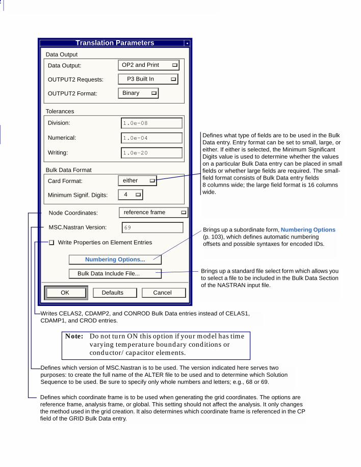
4
102
Defines what type of fields are to be used in the Bulk Data entry. Entry format can be set to small, large, or either. If either is selected, the Minimum Significant Digits value is used to determine whether the values on a particular Bulk Data entry can be placed in small fields or whether large fields are required. The small-field format consists of Bulk Data entry fields 8 columns wide; the large field format is 16 columns wide.
Brings up a subordinate form, Numbering Options (p. 103), which defines automatic numbering offsets and possible syntaxes for encoded IDs.
Translation Parameters
OP2 and PrintData Output:
P3 Built InOUTPUT2 Requests:
Binary OUTPUT2 Format:
Data Output
1.0e-08Division:
1.0e-04Numerical:
1.0e-20Writing:
Tolerances
either Card Format:
4Minimum Signif. Digits:
Bulk Data Format
reference frame Node Coordinates:
69MSC.Nastran Version:
Numbering Options...
Bulk Data Include File...
OK Defaults Cancel
Brings up a standard file select form which allows you to select a file to be included in the Bulk Data Section of the NASTRAN input file.
Write Properties on Element Entries
Defines which coordinate frame is to be used when generating the grid coordinates. The options are reference frame, analysis frame, or global. This setting should not affect the analysis. It only changes the method used in the grid creation. It also determines which coordinate frame is referenced in the CP field of the GRID Bulk Data entry.
Defines which version of MSC.Nastran is to be used. The version indicated here serves two purposes: to create the full name of the ALTER file to be used and to determine which Solution Sequence to be used. Be sure to specify only whole numbers and letters; e.g., 68 or 69.
Writes CELAS2, CDAMP2, and CONROD Bulk Data entries instead of CELAS1, CDAMP1, and CROD entries.
Note: Do not turn ON this option if your model has time varying temperature boundary conditions or conductor/capacitor elements.
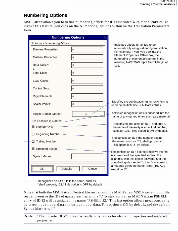
103CHAPTER 4Running a Thermal Analysis
4
Numbering OptionsMSC.Patran allows you to define numbering offsets for IDs associated with model entities. To invoke this feature, you click on the Numbering Options button on the Translation Parameters form.
Note that both the MSC.Patran Neutral file reader and the MSC.Patran MSC.Nastran input file reader preserve the IDS of named entities with a “.” syntax, so that an MSC.Nastran PSHELL entry of ID 12 will be assigned the name “PSHELL.12.” This last option allows great continuity between input model data and output model data. This option is ON by default, and the default Syntax Marker is “.”
Note: “The Encoded IDs” option currently only works for element properties and material properties.
Numbering Options
0Element Properties:
0Material Properties:
0Data Tables:
0Load Sets:
0Load Cases:
0Control Sets:
0Rigid Elements:
0Scalar Points:
Automatic Numbering Offsets:
+ ABegin. Contin. Marker:
Number Only
Beginning Number
Trailing Number
Encoded Syntax
.Syntax Marker:
IDs Encoded in Names:
OK Defaults Cancel
Recognizes an ID if it directly follows the first occurrence of the specified syntax. For example, with this option activated and the specified syntax set to “.”, the ID assigned to a material given the name “Steel_1027.32” would be 32.
Specifies the continuation mnemonic format used on multiple line Bulk Data entries.
Activates recognition of IDs encoded into the name of any named entry, such as a material.
Recognizes and uses an ID if, and only if, the name of the entity is an actual number, such as “105.” This option is ON by default.
Recognizes an ID if the number begins the name, such as “52_shell_property.” This option is OFF by default.
Recognizes an ID if it tails the name, such as “shell_property_52.” This option is OFF by default.
Indicates offsets for all IDs to be automatically assigned during translation. For example, if you type 100 into the Element Properties Offset box, the numbering of element properties in the resulting NASTRAN input file will begin at 101.
s:
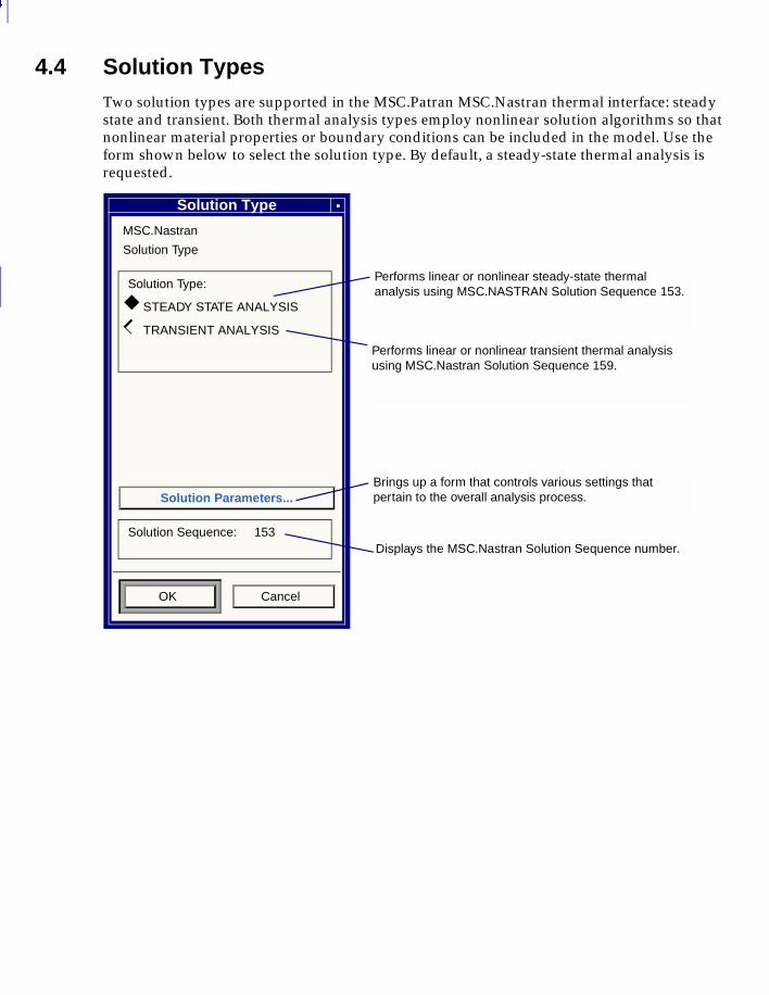
4
104
4.4 Solution TypesTwo solution types are supported in the MSC.Patran MSC.Nastran thermal interface: steady state and transient. Both thermal analysis types employ nonlinear solution algorithms so that nonlinear material properties or boundary conditions can be included in the model. Use the form shown below to select the solution type. By default, a steady-state thermal analysis is requested.
Solution Type
MSC.Nastran
Solution Type
Solution Type:
STEADY STATE ANALYSIS
TRANSIENT ANALYSIS
Solution Parameters...
Solution Sequence: 153
OK Cancel
Brings up a form that controls various settings that pertain to the overall analysis process.
Displays the MSC.Nastran Solution Sequence number.
Performs linear or nonlinear steady-state thermal analysis using MSC.NASTRAN Solution Sequence 153.
Performs linear or nonlinear transient thermal analysis using MSC.Nastran Solution Sequence 159.
◆
◆◆
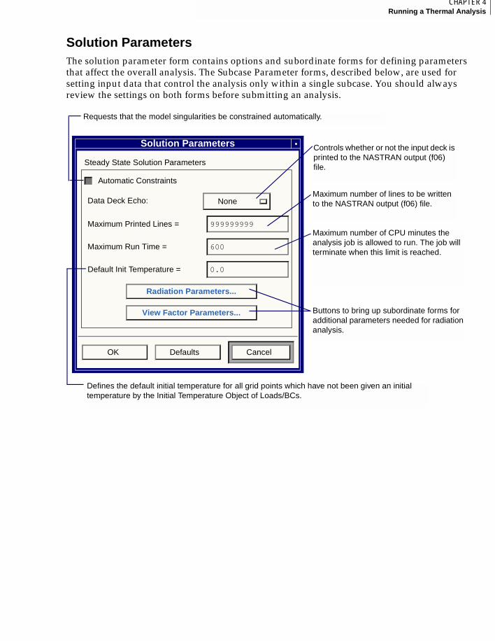
105CHAPTER 4Running a Thermal Analysis
4
Solution ParametersThe solution parameter form contains options and subordinate forms for defining parameters that affect the overall analysis. The Subcase Parameter forms, described below, are used for setting input data that control the analysis only within a single subcase. You should always review the settings on both forms before submitting an analysis.
Solution Parameters
Steady State Solution Parameters
Automatic Constraints
Data Deck Echo: None
Maximum Printed Lines = 999999999
Maximum Run Time = 600
Default Init Temperature = 0.0
Radiation Parameters...
View Factor Parameters...
OK Defaults Cancel
Controls whether or not the input deck is printed to the NASTRAN output (f06) file.
Maximum number of lines to be written to the NASTRAN output (f06) file.
Maximum number of CPU minutes the analysis job is allowed to run. The job will terminate when this limit is reached.
Buttons to bring up subordinate forms for additional parameters needed for radiation analysis.
Requests that the model singularities be constrained automatically.
Defines the default initial temperature for all grid points which have not been given an initial temperature by the Initial Temperature Object of Loads/BCs.
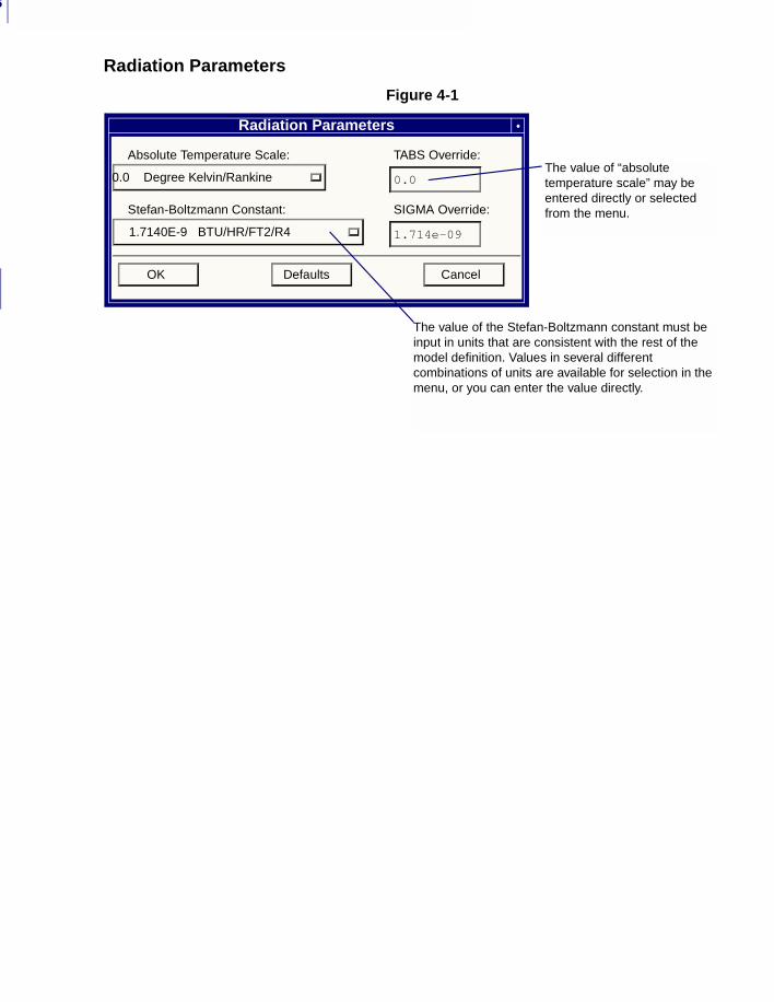
4
106
Radiation Parameters
Figure 4-1
Radiation Parameters
Absolute Temperature Scale:
0.0 Degree Kelvin/Rankine
TABS Override:
0.0
Stefan-Boltzmann Constant:
1.7140E-9 BTU/HR/FT2/R4
SIGMA Override:
1.714e-09
OK Defaults Cancel
The value of the Stefan-Boltzmann constant must be input in units that are consistent with the rest of the model definition. Values in several different combinations of units are available for selection in the menu, or you can enter the value directly.
The value of “absolute temperature scale” may be entered directly or selected from the menu.
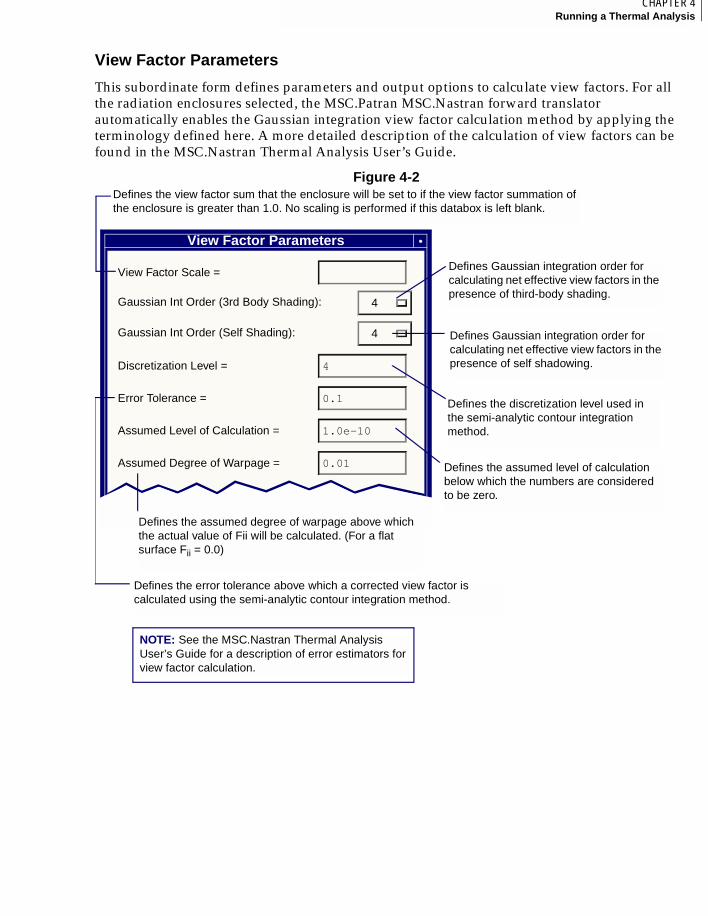
107CHAPTER 4Running a Thermal Analysis
4
View Factor Parameters
This subordinate form defines parameters and output options to calculate view factors. For all the radiation enclosures selected, the MSC.Patran MSC.Nastran forward translator automatically enables the Gaussian integration view factor calculation method by applying the terminology defined here. A more detailed description of the calculation of view factors can be found in the MSC.Nastran Thermal Analysis User’s Guide.
Figure 4-2
View Factor Parameters
View Factor Scale =
Gaussian Int Order (3rd Body Shading): 4
Gaussian Int Order (Self Shading): 4
Discretization Level = 4
Error Tolerance = 0.1
Assumed Level of Calculation = 1.0e-10
Assumed Degree of Warpage = 0.01
Defines the view factor sum that the enclosure will be set to if the view factor summation of the enclosure is greater than 1.0. No scaling is performed if this databox is left blank.
Defines Gaussian integration order for calculating net effective view factors in the presence of third-body shading.
Defines Gaussian integration order for calculating net effective view factors in the presence of self shadowing.
Defines the discretization level used in the semi-analytic contour integration method.
Defines the error tolerance above which a corrected view factor is calculated using the semi-analytic contour integration method.
Defines the assumed level of calculation below which the numbers are considered to be zero.
Defines the assumed degree of warpage above which the actual value of Fii will be calculated. (For a flat surface Fii = 0.0)
NOTE: See the MSC.Nastran Thermal Analysis User’s Guide for a description of error estimators for view factor calculation.
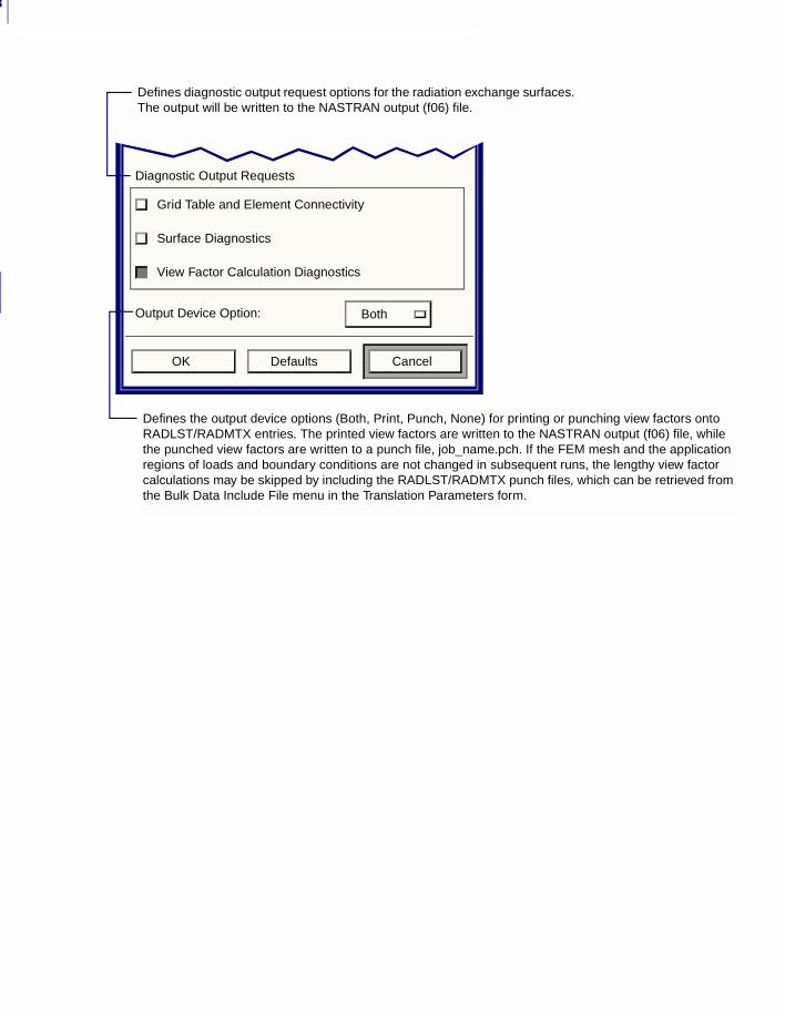
4
108
Diagnostic Output Requests
Grid Table and Element Connectivity
Surface Diagnostics
View Factor Calculation Diagnostics
Output Device Option: Both
OK Defaults Cancel
Defines the output device options (Both, Print, Punch, None) for printing or punching view factors onto RADLST/RADMTX entries. The printed view factors are written to the NASTRAN output (f06) file, while the punched view factors are written to a punch file, job_name.pch. If the FEM mesh and the application regions of loads and boundary conditions are not changed in subsequent runs, the lengthy view factor calculations may be skipped by including the RADLST/RADMTX punch files, which can be retrieved from the Bulk Data Include File menu in the Translation Parameters form.
Defines diagnostic output request options for the radiation exchange surfaces. The output will be written to the NASTRAN output (f06) file.
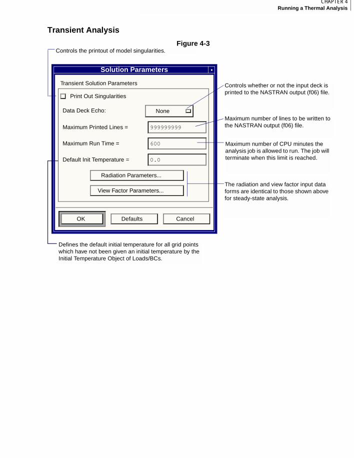
109CHAPTER 4Running a Thermal Analysis
4
Transient Analysis
Figure 4-3
Solution Parameters
Transient Solution Parameters
Print Out Singularities
Data Deck Echo: None
Maximum Printed Lines = 999999999
Maximum Run Time = 600
Default Init Temperature = 0.0
Radiation Parameters...
View Factor Parameters...
OK Defaults Cancel
The radiation and view factor input data forms are identical to those shown above for steady-state analysis.
Controls whether or not the input deck is printed to the NASTRAN output (f06) file.
Maximum number of lines to be written to the NASTRAN output (f06) file.
Maximum number of CPU minutes the analysis job is allowed to run. The job will terminate when this limit is reached.
Controls the printout of model singularities.
Defines the default initial temperature for all grid points which have not been given an initial temperature by the Initial Temperature Object of Loads/BCs.
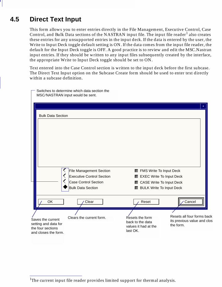
4
110
4.5 Direct Text InputThis form allows you to enter entries directly in the File Management, Executive Control, Case Control, and Bulk Data sections of the NASTRAN input file. The input file reader1 also creates these entries for any unsupported entries in the input deck. If the data is entered by the user, the Write to Input Deck toggle default setting is ON. If the data comes from the input file reader, the default for the Input Deck toggle is OFF. A good practice is to review and edit the MSC.Nastran input entries. If they should be written to any input files subsequently created by the interface, the appropriate Write to Input Deck toggle should be set to ON.
Text entered into the Case Control section is written to the input deck before the first subcase. The Direct Text Input option on the Subcase Create form should be used to enter text directly within a subcase definition.
1The current input file reader provides limited support for thermal analysis.
Direct Text Input
Bulk Data Section
File Management Section
Executive Control Section
Case Control Section
Bulk Data Section
FMS Write To Input Deck
EXEC Write To Input Deck
CASE Write To Input Deck
BULK Write To Input Deck
OK Clear Reset Cancel
Switches to determine which data section the MSC ⁄NASTRAN input would be sent.
Saves the current setting and data for the four sections and closes the form.
Clears the current form. Resets the form back to the data values it had at the last OK.
Resets all four forms back its previous value and closthe form.
◆◆
◆◆
◆◆
◆
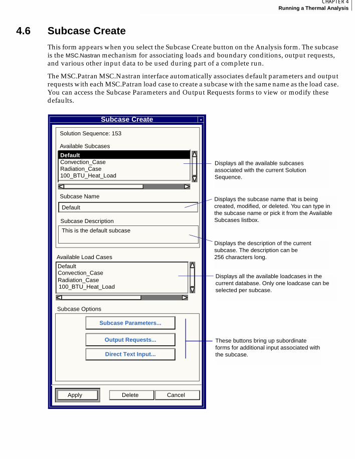
111CHAPTER 4Running a Thermal Analysis
4
4.6 Subcase CreateThis form appears when you select the Subcase Create button on the Analysis form. The subcase is the MSC.Nastran mechanism for associating loads and boundary conditions, output requests, and various other input data to be used during part of a complete run.
The MSC.Patran MSC.Nastran interface automatically associates default parameters and output requests with each MSC.Patran load case to create a subcase with the same name as the load case. You can access the Subcase Parameters and Output Requests forms to view or modify these defaults.
Subcase Create
Solution Sequence: 153
Available Subcases
Convection_Case
Radiation_Case100_BTU_Heat_Load
Subcase Name
Subcase Description
Available Load Cases
Default
Subcase Options
Apply Delete Cancel
Subcase Parameters...
Output Requests...
Direct Text Input...
Default
Default
This is the default subcase
Displays all the available subcases associated with the current Solution Sequence.
Displays the subcase name that is being created, modified, or deleted. You can type in the subcase name or pick it from the Available Subcases listbox.
Displays the description of the current subcase. The description can be 256 characters long.
Displays all the available loadcases in the current database. Only one loadcase can be selected per subcase.
Convection_Case
Radiation_Case
These buttons bring up subordinate forms for additional input associated with the subcase.
100_BTU_Heat_Load
4
112
Subcase ParametersThe controls and parameters set on the Subcase Parameters forms apply to a single MSC.Nastran subcase within the overall analysis run.
Steady-State Subcase
This subordinate form appears when the Subcase Parameters button is selected on the Subcase Create form and the solution type is Steady State. This form provides for the definition of the input data that controls the solution of the nonlinear equations.
Occasionally, when solving a set of nonlinear equations, it may not be possible to obtain a solution directly with the total heat load applied. Instead, the solution is obtained by applying the loading in increments, solving the system equations for the current fraction of the total load, and using that solution as the starting point for the next increment of load. This process continues until the desired total heat load is applied. It should be mentioned that the number of load increments has no effect on the accuracy of the solution-- it is merely a computational technique to aid in obtaining the solution efficiently. In linear or mildly nonlinear problems, a single increment is usually applied. In highly nonlinear problems, dozens of increments may be required to obtain a converged solution.
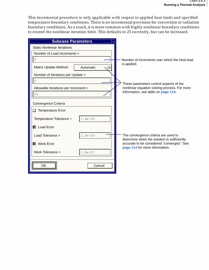
113CHAPTER 4Running a Thermal Analysis
4
This incremental procedure is only applicable with respect to applied heat loads and specified temperature boundary conditions. There is no incremental provision for convection or radiation boundary conditions. As a result, it is more common with highly nonlinear boundary conditions to exceed the nonlinear iteration limit. This defaults to 25 currently, but can be increased.
Subcase ParametersStatic Nonlinear Iterations
Number of Load Increments =
0
Matrix Update Method: Automatic
Number of Iterations per Update =
5
Allowable Iterations per Increment =
25
Convergence Criteria
Temperature Error
Temperature Tolerance = 1.0e-03
Load Error
Load Tolerance = 1.0e-03
Work Error
Work Tolerance = 1.0e-07
OK Cancel
Number of increments over which the heat load is applied.
These parameters control aspects of the nonlinear equation solving process. For more information, see table on page 114.
The convergence criteria are used to determine when the solution is sufficiently accurate to be considered “converged.” See page 114 for more information.
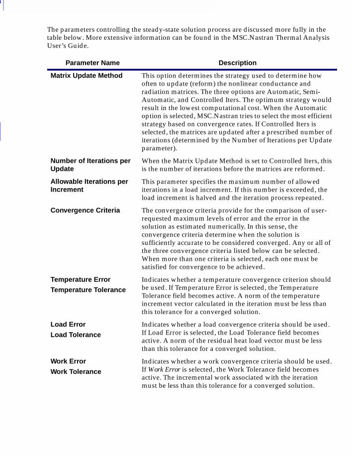
4
114
The parameters controlling the steady-state solution process are discussed more fully in the table below. More extensive information can be found in the MSC.Nastran Thermal Analysis User’s Guide.
Parameter Name Description
Matrix Update Method This option determines the strategy used to determine how often to update (reform) the nonlinear conductance and radiation matrices. The three options are Automatic, Semi-Automatic, and Controlled Iters. The optimum strategy would result in the lowest computational cost. When the Automatic option is selected, MSC.Nastran tries to select the most efficient strategy based on convergence rates. If Controlled Iters is selected, the matrices are updated after a prescribed number of iterations (determined by the Number of Iterations per Update parameter).
Number of Iterations per Update
When the Matrix Update Method is set to Controlled Iters, this is the number of iterations before the matrices are reformed.
Allowable Iterations per Increment
This parameter specifies the maximum number of allowed iterations in a load increment. If this number is exceeded, the load increment is halved and the iteration process repeated.
Convergence Criteria The convergence criteria provide for the comparison of user-requested maximum levels of error and the error in the solution as estimated numerically. In this sense, the convergence criteria determine when the solution is sufficiently accurate to be considered converged. Any or all of the three convergence criteria listed below can be selected. When more than one criteria is selected, each one must be satisfied for convergence to be achieved.
Temperature Error
Temperature Tolerance
Indicates whether a temperature convergence criterion should be used. If Temperature Error is selected, the Temperature Tolerance field becomes active. A norm of the temperature increment vector calculated in the iteration must be less than this tolerance for a converged solution.
Load Error
Load Tolerance
Indicates whether a load convergence criteria should be used. If Load Error is selected, the Load Tolerance field becomes active. A norm of the residual heat load vector must be less than this tolerance for a converged solution.
Work Error
Work Tolerance
Indicates whether a work convergence criteria should be used. If Work Error is selected, the Work Tolerance field becomes active. The incremental work associated with the iteration must be less than this tolerance for a converged solution.
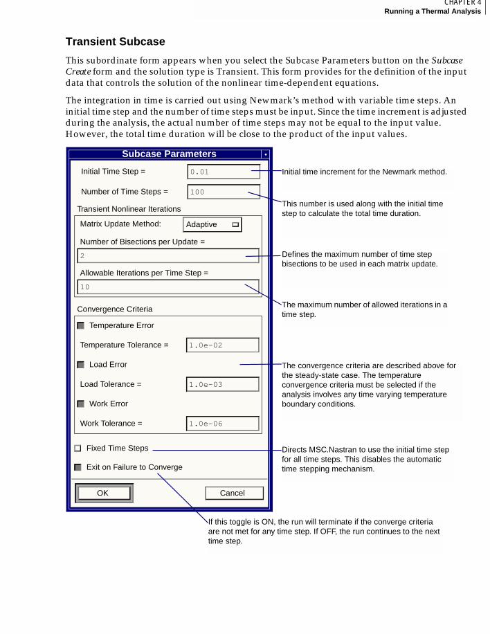
115CHAPTER 4Running a Thermal Analysis
4
Transient Subcase
This subordinate form appears when you select the Subcase Parameters button on the Subcase Create form and the solution type is Transient. This form provides for the definition of the input data that controls the solution of the nonlinear time-dependent equations.
The integration in time is carried out using Newmark’s method with variable time steps. An initial time step and the number of time steps must be input. Since the time increment is adjusted during the analysis, the actual number of time steps may not be equal to the input value. However, the total time duration will be close to the product of the input values.
Subcase Parameters
Initial Time Step = 0.01
Number of Time Steps = 100
Transient Nonlinear Iterations
Matrix Update Method: Adaptive
Number of Bisections per Update =
2
Allowable Iterations per Time Step =
10
Convergence Criteria
Temperature Error
Temperature Tolerance = 1.0e-02
Load Error
Load Tolerance = 1.0e-03
Work Error
Work Tolerance = 1.0e-06
Fixed Time Steps
Exit on Failure to Converge
OK Cancel
Initial time increment for the Newmark method.
This number is used along with the initial time step to calculate the total time duration.
If this toggle is ON, the run will terminate if the converge criteria are not met for any time step. If OFF, the run continues to the next time step.
Directs MSC.Nastran to use the initial time step for all time steps. This disables the automatic time stepping mechanism.
The convergence criteria are described above for the steady-state case. The temperature convergence criteria must be selected if the analysis involves any time varying temperature boundary conditions.
Defines the maximum number of time step bisections to be used in each matrix update.
The maximum number of allowed iterations in a time step.
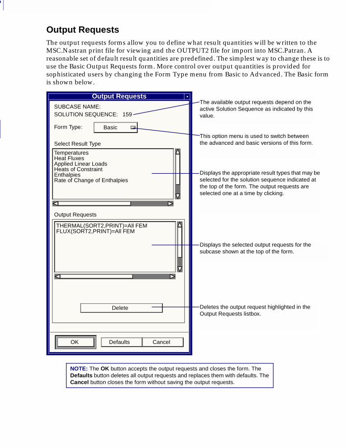
4
116
Output RequestsThe output requests forms allow you to define what result quantities will be written to the MSC.Nastran print file for viewing and the OUTPUT2 file for import into MSC.Patran. A reasonable set of default result quantities are predefined. The simplest way to change these is to use the Basic Output Requests form. More control over output quantities is provided for sophisticated users by changing the Form Type menu from Basic to Advanced. The Basic form is shown below.
Output RequestsSUBCASE NAME: SOLUTION SEQUENCE: 159
Form Type: Basic
Select Result Type
TemperaturesHeat FluxesApplied Linear LoadsHeats of ConstraintEnthalpiesRate of Change of Enthalpies
Output Requests
THERMAL(SORT2,PRINT)=All FEMFLUX(SORT2,PRINT)=All FEM
Delete
OK Defaults Cancel
The available output requests depend on the active Solution Sequence as indicated by this value.
Displays the appropriate result types that may be selected for the solution sequence indicated at the top of the form. The output requests are selected one at a time by clicking.
Displays the selected output requests for the subcase shown at the top of the form.
This option menu is used to switch between the advanced and basic versions of this form.
Deletes the output request highlighted in the Output Requests listbox.
NOTE: The OK button accepts the output requests and closes the form. The Defaults button deletes all output requests and replaces them with defaults. The Cancel button closes the form without saving the output requests.
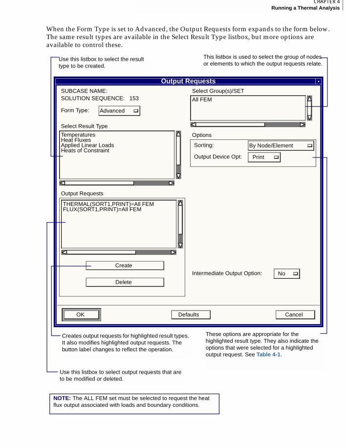
117CHAPTER 4Running a Thermal Analysis
4
When the Form Type is set to Advanced, the Output Requests form expands to the form below. The same result types are available in the Select Result Type listbox, but more options are available to control these.
Output RequestsSUBCASE NAME: SOLUTION SEQUENCE: 153
Form Type: Advanced
Select Result Type
TemperaturesHeat FluxesApplied Linear LoadsHeats of Constraint
Output Requests
THERMAL(SORT1,PRINT)=All FEMFLUX(SORT1,PRINT)=All FEM
Create
Delete
OK Defaults Cancel
Select Group(s)/SET
All FEM
Options
Sorting: By Node/Element
Output Device Opt: Print
Intermediate Output Option: No
This listbox is used to select the group of nodes or elements to which the output requests relate.
Use this listbox to select the result type to be created.
These options are appropriate for the highlighted result type. They also indicate the options that were selected for a highlighted output request. See Table 4-1.
Use this listbox to select output requests that are to be modified or deleted.
Creates output requests for highlighted result types. It also modifies highlighted output requests. The button label changes to reflect the operation.
NOTE: The ALL FEM set must be selected to request the heat flux output associated with loads and boundary conditions.
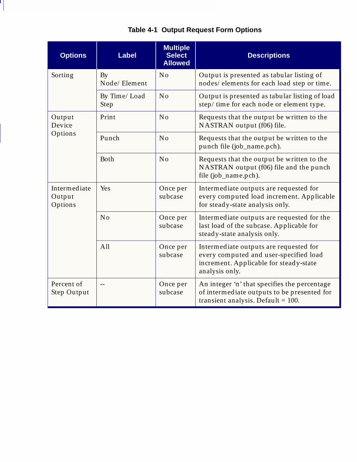
4
118
Table 4-1 Output Request Form Options
Options LabelMultiple Select
AllowedDescriptions
Sorting By Node/Element
No Output is presented as tabular listing of nodes/elements for each load step or time.
By Time/Load Step
No Output is presented as tabular listing of load step/time for each node or element type.
Output Device Options
Print No Requests that the output be written to the NASTRAN output (f06) file.
Punch No Requests that the output be written to the punch file (job_name.pch).
Both No Requests that the output be written to the NASTRAN output (f06) file and the punch file (job_name.pch).
IntermediateOutput Options
Yes Once per subcase
Intermediate outputs are requested for every computed load increment. Applicable for steady-state analysis only.
No Once per subcase
Intermediate outputs are requested for the last load of the subcase. Applicable for steady-state analysis only.
All Once per subcase
Intermediate outputs are requested for every computed and user-specified load increment. Applicable for steady-state analysis only.
Percent of Step Output
-- Once per subcase
An integer ‘n’ that specifies the percentage of intermediate outputs to be presented for transient analysis. Default = 100.
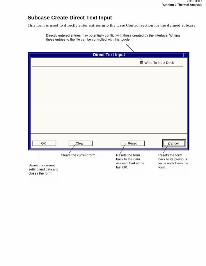
119CHAPTER 4Running a Thermal Analysis
4
Subcase Create Direct Text InputThis form is used to directly enter entries into the Case Control section for the defined subcase.
Direct Text Input
Write To Input Deck
OK Clear Reset Cancel
Directly entered entries may potentially conflict with those created by the interface. Writing these entries to the file can be controlled with this toggle.
Saves the current setting and data and closes the form.
Clears the current form. Resets the form back to the data values it had at the last OK.
Resets the form back to its previous value and closes the form.
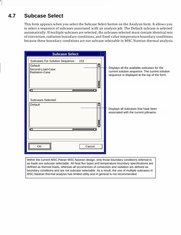
4
120
4.7 Subcase SelectThis form appears when you select the Subcase Select button on the Analysis form. It allows you to select a sequence of subcases associated with an analysis job. The Default subcase is selected automatically. If multiple subcases are selected, the subcases selected must contain identical sets of convection, radiation boundary conditions, and fixed value temperature boundary conditions because these boundary conditions are not subcase selectable in MSC.Nastran thermal analysis.
Displays all the available subcases for the current solution sequence. The current solution sequence is displayed at the top of the form.
Displays all subcases that have been associated with the current jobname.
Subcase Select
Subcases For Solution Sequence: 153
Default
Subcases Selected:
Default
OK Cancel
Second-Load-Case Radiation-Case
Within the current MSC.Patran MSC.Nastran design, only those boundary conditions referred to as loads are subcase selectable. All heat flux types and temperature boundary specifications are defined as thermal loads, whereas all occurrences of convection and radiation are defined as boundary conditions and are not subcase selectable. As a result, the use of multiple subcases in MSC.Nastran thermal analysis has limited utility and in general is not recommended.
MSC.Patran MSC.Nastran Preference Guide, Volume 2: Thermal Analysis
CHAPTER
5 Results Processing and Visualization
■ Overview
■ Reading Thermal Analysis Results
■ Results Visualization Options
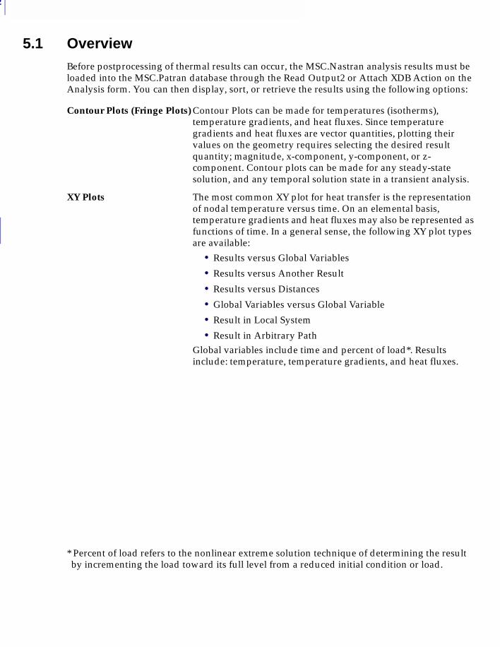
5
122
5.1 OverviewBefore postprocessing of thermal results can occur, the MSC.Nastran analysis results must be loaded into the MSC.Patran database through the Read Output2 or Attach XDB Action on the Analysis form. You can then display, sort, or retrieve the results using the following options:
Contour Plots (Fringe Plots) Contour Plots can be made for temperatures (isotherms), temperature gradients, and heat fluxes. Since temperature gradients and heat fluxes are vector quantities, plotting their values on the geometry requires selecting the desired result quantity; magnitude, x-component, y-component, or z-component. Contour plots can be made for any steady-state solution, and any temporal solution state in a transient analysis.
XY Plots The most common XY plot for heat transfer is the representation of nodal temperature versus time. On an elemental basis, temperature gradients and heat fluxes may also be represented as functions of time. In a general sense, the following XY plot types are available:
• Results versus Global Variables
• Results versus Another Result
• Results versus Distances
• Global Variables versus Global Variable
• Result in Local System
• Result in Arbitrary PathGlobal variables include time and percent of load*. Results include: temperature, temperature gradients, and heat fluxes.
* Percent of load refers to the nonlinear extreme solution technique of determining the result by incrementing the load toward its full level from a reduced initial condition or load.
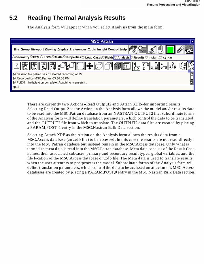
123CHAPTER 5Results Processing and Visualization
5
5.2 Reading Thermal Analysis ResultsThe Analysis form will appear when you select Analysis from the main form.
There are currently two Actions--Read Output2 and Attach XDB--for importing results. Selecting Read Output2 as the Action on the Analysis form allows the model and⁄or results data to be read into the MSC.Patran database from an NASTRAN OUTPUT2 file. Subordinate forms of the Analysis form will define translation parameters, which control the data to be translated, and the OUTPUT2 file from which to translate. The OUTPUT2 data files are created by placing a PARAM,POST,-1 entry in the MSC.Nastran Bulk Data section.
Selecting Attach XDB as the Action on the Analysis form allows the results data from a MSC.Access database (an .xdb file) to be accessed. In this case the results are not read directly into the MSC.Patran database but instead remain in the MSC.Access database. Only what is termed as meta data is read into the MSC.Patran database. Meta data consists of the Result Case names, their associated subcases, primary and secondary result types, global variables, and the file location of the MSC.Access database or .xdb file. The Meta data is used to translate results when the user attempts to postprocess the model. Subordinate forms of the Analysis form will define translation parameters, which control the data to be accessed on attachment. MSC.Access databases are created by placing a PARAM,POST,0 entry in the MSC.Nastran Bulk Data section.
MSC.Patran
hp, 2
$# Session file patran.ses.01 started recording at 25$# Recorded by MSC.Patran 03:36:58 PM$# FLEXlm Initialization complete. Acquiring license(s)...
File Group Viewport Display Preferences Tools HelpInsight Control
Geometry© FEM LBCs Matls Properties© ©© © Load Cases© Fields Analysis Results Insight© ©© © XYPlot©
Viewing
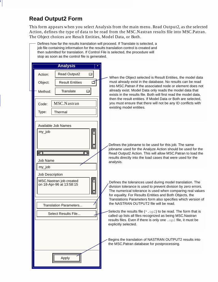
5
124
Read Output2 FormThis form appears when you select Analysis from the main menu. Read Output2, as the selected Action, defines the type of data to be read from the MSC.Nastran results file into MSC.Patran. The Object choices are Result Entities, Model Data, or Both.
When the Object selected is Result Entities, the model data must already exist in the database. No results can be read into MSC.Patran if the associated node or element does not already exist. Model Data only reads the model data that exists in the results file. Both will first read the model data, then the result entities. If Model Data or Both are selected, you must ensure that there will not be any ID conflicts with existing model entities.
Defines the jobname to be used for this job. The same jobname used for the Analyze Action should be used for the Read Output2 Action. This will allow MSC.Patran to load the results directly into the load cases that were used for the analysis.
Analysis
Read Output2Action:
Result EntitiesObject:
TranslateMethod:
Translation Parameters...
Select Results File...
Apply
Selects the results file (*.op2) to be read. The form that is called up lists all files recognized as being MSC.Nastran results files. Even if there is only one .op2 file, it must be explicitly selected.
Defines how far the results translation will proceed. If Translate is selected, a job file containing information for the results translation control is created and then submitted for translation. If Control File is selected, the procedure will stop as soon as the control file is generated.
Defines the tolerances used during model translation. The division tolerance is used to prevent division by zero errors. The numerical tolerance is used when comparing real values for equality. For Results Entities and Both Objects, the Translations Parameters form also specifies which version of the NASTRAN OUTPUT2 file will be read.
Available Job Names
Code:
Type:
Job Name
Job Description
MSC.Nastran
Thermal
my_job
MSC.Nastran job createdon 18-Apr-96 at 13:58:15
my_job
Begins the translation of NASTRAN OUTPUT2 results into the MSC.Patran database for postprocessing.
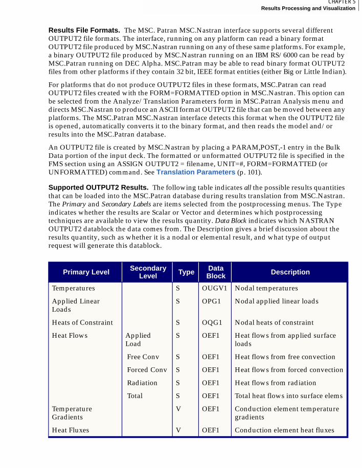
125CHAPTER 5Results Processing and Visualization
5
Results File Formats. The MSC. Patran MSC.Nastran interface supports several different OUTPUT2 file formats. The interface, running on any platform can read a binary format OUTPUT2 file produced by MSC.Nastran running on any of these same platforms. For example, a binary OUTPUT2 file produced by MSC.Nastran running on an IBM RS/6000 can be read by MSC.Patran running on DEC Alpha. MSC.Patran may be able to read binary format OUTPUT2 files from other platforms if they contain 32 bit, IEEE format entities (either Big or Little Indian).
For platforms that do not produce OUTPUT2 files in these formats, MSC.Patran can read OUTPUT2 files created with the FORM=FORMATTED option in MSC.Nastran. This option can be selected from the Analyze/Translation Parameters form in MSC.Patran Analysis menu and directs MSC.Nastran to produce an ASCII format OUTPUT2 file that can be moved between any platforms. The MSC.Patran MSC.Nastran interface detects this format when the OUTPUT2 file is opened, automatically converts it to the binary format, and then reads the model and/or results into the MSC.Patran database.
An OUTPUT2 file is created by MSC.Nastran by placing a PARAM,POST,-1 entry in the Bulk Data portion of the input deck. The formatted or unformatted OUTPUT2 file is specified in the FMS section using an ASSIGN OUTPUT2 = filename, UNIT=#, FORM=FORMATTED (or UNFORMATTED) command. See Translation Parameters (p. 101).
Supported OUTPUT2 Results. The following table indicates all the possible results quantities that can be loaded into the MSC.Patran database during results translation from MSC.Nastran. The Primary and Secondary Labels are items selected from the postprocessing menus. The Type indicates whether the results are Scalar or Vector and determines which postprocessing techniques are available to view the results quantity. Data Block indicates which NASTRAN OUTPUT2 datablock the data comes from. The Description gives a brief discussion about the results quantity, such as whether it is a nodal or elemental result, and what type of output request will generate this datablock.
Primary Level Secondary Level Type Data
Block Description
Temperatures S OUGV1 Nodal temperatures
Applied Linear Loads
S OPG1 Nodal applied linear loads
Heats of Constraint S OQG1 Nodal heats of constraint
Heat Flows Applied Load
S OEF1 Heat flows from applied surface loads
Free Conv S OEF1 Heat flows from free convection
Forced Conv S OEF1 Heat flows from forced convection
Radiation S OEF1 Heat flows from radiation
Total S OEF1 Total heat flows into surface elems
Temperature Gradients
V OEF1 Conduction element temperature gradients
Heat Fluxes V OEF1 Conduction element heat fluxes
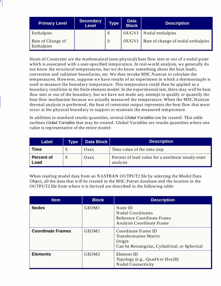
5
126
Heats of Constraint are the mathematical (non-physical) heat flow into or out of a nodal point which is associated with a user-specified temperature. In real-world analysis, we generally do not know the structural temperatures, but we do know something about the heat loads, convection and radiation boundaries, etc. We then invoke MSC.Nastran to calculate the temperatures. However, suppose we have results of an experiment in which a thermocouple is used to measure the boundary temperature. This temperature could then be applied as a boundary condition in the finite element model. In the experimental test, there may well be heat flow into or out of the boundary, but we have not made any attempt to qualify or quantify the heat flow mechanism because we actually measured the temperature. When the MSC.Nastran thermal analysis is performed, the heat of constraint output represents the heat flow that must occur at the physical boundary to support or maintain the measured temperature.
In addition to standard results quantities, several Global Variables can be created. This table outlines Global Variables that may be created. Global Variables are results quantities where one value is representative of the entire model:
When reading model data from an NASTRAN OUTPUT2 file by selecting the Model Data Object, all the data that will be created in the MSC.Patran database and the location in the OUTPUT2 file from where it is derived are described in the following table:
Enthalpies S OUGV1 Nodal enthalpies
Rate of Change of Enthalpies
S OUGV1 Rate of change of nodal enthalpies
Label Type Data Block Description
Time S Oxxx Time value of the time step
Percent of Load
S Oxxx Percent of load value for a nonlinear steady-state analysis
Item Block Description
Nodes GEOM1 Node IDNodal CoordinatesReference Coordinate FrameAnalysis Coordinate Frame
Coordinate Frames GEOM1 Coordinate Frame IDTransformation MatrixOriginCan be Rectangular, Cylindrical, or Spherical
Elements GEOM2 Element IDTopology (e.g., Quad4 or Hex20)Nodal Connectivity
Primary Level Secondary Level Type Data
Block Description
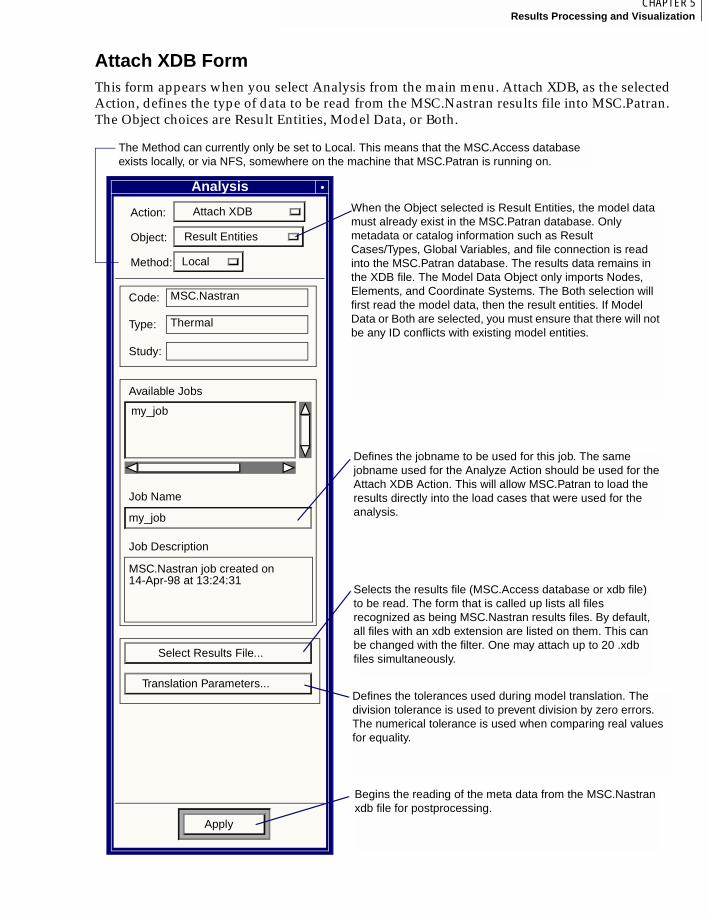
127CHAPTER 5Results Processing and Visualization
5
Attach XDB FormThis form appears when you select Analysis from the main menu. Attach XDB, as the selected Action, defines the type of data to be read from the MSC.Nastran results file into MSC.Patran. The Object choices are Result Entities, Model Data, or Both.
When the Object selected is Result Entities, the model data must already exist in the MSC.Patran database. Only metadata or catalog information such as Result Cases/Types, Global Variables, and file connection is read into the MSC.Patran database. The results data remains in the XDB file. The Model Data Object only imports Nodes, Elements, and Coordinate Systems. The Both selection will first read the model data, then the result entities. If Model Data or Both are selected, you must ensure that there will not be any ID conflicts with existing model entities.
Defines the jobname to be used for this job. The same jobname used for the Analyze Action should be used for the Attach XDB Action. This will allow MSC.Patran to load the results directly into the load cases that were used for the analysis.
Selects the results file (MSC.Access database or xdb file) to be read. The form that is called up lists all files recognized as being MSC.Nastran results files. By default, all files with an xdb extension are listed on them. This can be changed with the filter. One may attach up to 20 .xdb files simultaneously.
The Method can currently only be set to Local. This means that the MSC.Access database exists locally, or via NFS, somewhere on the machine that MSC.Patran is running on.
Begins the reading of the meta data from the MSC.Nastran xdb file for postprocessing.
Analysis
Action: Attach XDB
Object: Result Entities
Method: Local
Code:
Type:
Study:
MSC.Nastran
Thermal
Available Jobs
Job Name
my_job
Job Description
MSC.Nastran job created on
Select Results File...
Translation Parameters...
Apply
14-Apr-98 at 13:24:31
my_job
Defines the tolerances used during model translation. The division tolerance is used to prevent division by zero errors. The numerical tolerance is used when comparing real values for equality.
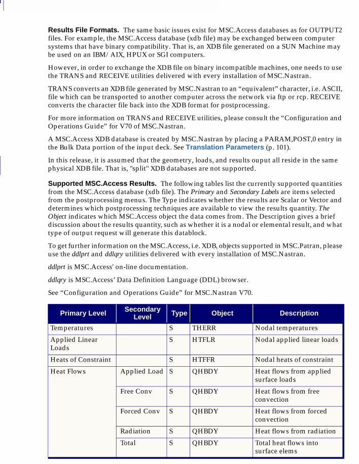
5
128
Results File Formats. The same basic issues exist for MSC.Access databases as for OUTPUT2 files. For example, the MSC.Access database (xdb file) may be exchanged between computer systems that have binary compatibility. That is, an XDB file generated on a SUN Machine may be used on an IBM/AIX, HPUX or SGI computers.
However, in order to exchange the XDB file on binary incompatible machines, one needs to use the TRANS and RECEIVE utilities delivered with every installation of MSC.Nastran.
TRANS converts an XDB file generated by MSC.Nastran to an “equivalent” character, i.e. ASCII, file which can be transported to another computer across the network via ftp or rcp. RECEIVE converts the character file back into the XDB format for postprocessing.
For more information on TRANS and RECEIVE utilities, please consult the “Configuration and Operations Guide” for V70 of MSC.Nastran.
A MSC.Access XDB database is created by MSC.Nastran by placing a PARAM,POST,0 entry in the Bulk Data portion of the input deck. See Translation Parameters (p. 101).
In this release, it is assumed that the geometry, loads, and results ouput all reside in the same physical XDB file. That is, "split" XDB databases are not supported.
Supported MSC.Access Results. The following tables list the currently supported quantities from the MSC.Access database (xdb file). The Primary and Secondary Labels are items selected from the postprocessing menus. The Type indicates whether the results are Scalar or Vector and determines which postprocessing techniques are available to view the results quantity. The Object indicates which MSC.Access object the data comes from. The Description gives a brief discussion about the results quantity, such as whether it is a nodal or elemental result, and what type of output request will generate this datablock.
To get further information on the MSC.Access, i.e. XDB, objects supported in MSC.Patran, please use the ddlprt and ddlqry utilities delivered with every installation of MSC.Nastran.
ddlprt is MSC.Access' on-line documentation.
ddlqry is MSC.Access’ Data Definition Language (DDL) browser.
See “Configuration and Operations Guide” for MSC.Nastran V70.
Primary Level Secondary Level Type Object Description
Temperatures S THERR Nodal temperatures
Applied Linear Loads
S HTFLR Nodal applied linear loads
Heats of Constraint S HTFFR Nodal heats of constraint
Heat Flows Applied Load S QHBDY Heat flows from applied surface loads
Free Conv S QHBDY Heat flows from free convection
Forced Conv S QHBDY Heat flows from forced convection
Radiation S QHBDY Heat flows from radiation
Total S QHBDY Total heat flows into surface elems
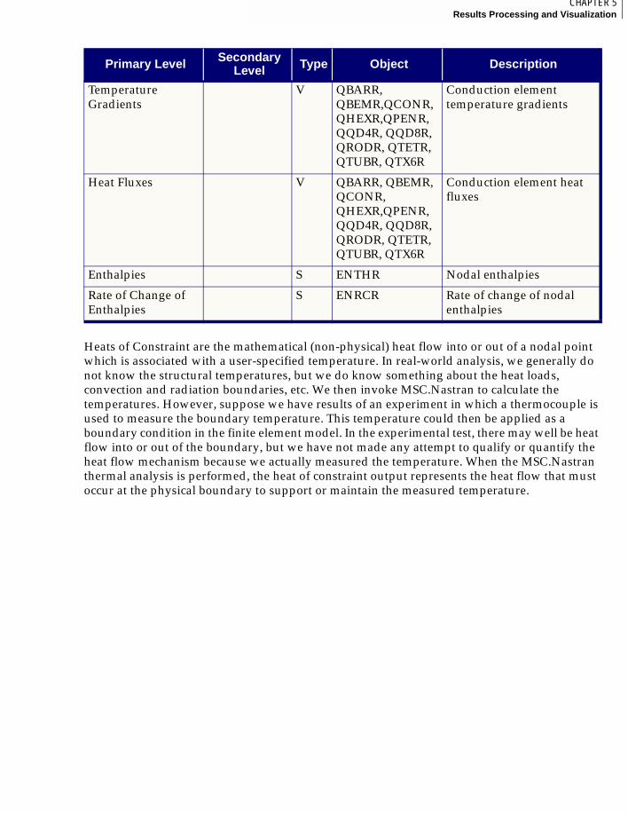
129CHAPTER 5Results Processing and Visualization
5
Heats of Constraint are the mathematical (non-physical) heat flow into or out of a nodal point which is associated with a user-specified temperature. In real-world analysis, we generally do not know the structural temperatures, but we do know something about the heat loads, convection and radiation boundaries, etc. We then invoke MSC.Nastran to calculate the temperatures. However, suppose we have results of an experiment in which a thermocouple is used to measure the boundary temperature. This temperature could then be applied as a boundary condition in the finite element model. In the experimental test, there may well be heat flow into or out of the boundary, but we have not made any attempt to qualify or quantify the heat flow mechanism because we actually measured the temperature. When the MSC.Nastran thermal analysis is performed, the heat of constraint output represents the heat flow that must occur at the physical boundary to support or maintain the measured temperature.
Temperature Gradients
V QBARR, QBEMR,QCONR, QHEXR,QPENR, QQD4R, QQD8R, QRODR, QTETR, QTUBR, QTX6R
Conduction element temperature gradients
Heat Fluxes V QBARR, QBEMR, QCONR, QHEXR,QPENR, QQD4R, QQD8R, QRODR, QTETR, QTUBR, QTX6R
Conduction element heat fluxes
Enthalpies S ENTHR Nodal enthalpies
Rate of Change of Enthalpies
S ENRCR Rate of change of nodal enthalpies
Primary Level Secondary Level Type Object Description
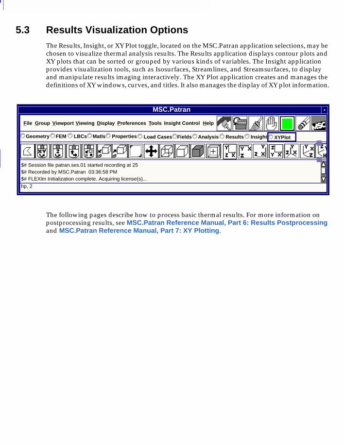
5
130
5.3 Results Visualization OptionsThe Results, Insight, or XY Plot toggle, located on the MSC.Patran application selections, may be chosen to visualize thermal analysis results. The Results application displays contour plots and XY plots that can be sorted or grouped by various kinds of variables. The Insight application provides visualization tools, such as Isosurfaces, Streamlines, and Streamsurfaces, to display and manipulate results imaging interactively. The XY Plot application creates and manages the definitions of XY windows, curves, and titles. It also manages the display of XY plot information.
The following pages describe how to process basic thermal results. For more information on postprocessing results, see MSC.Patran Reference Manual, Part 6: Results Postprocessing and MSC.Patran Reference Manual, Part 7: XY Plotting.
MSC.Patran
hp, 2
$# Session file patran.ses.01 started recording at 25$# Recorded by MSC.Patran 03:36:58 PM$# FLEXlm Initialization complete. Acquiring license(s)...
File Group Viewport Display Preferences Tools HelpInsight Control
Geometry© FEM LBCs Matls Properties© ©© © Load Cases© Fields Analysis Results Insight© ©© © XYPlot©
Viewing
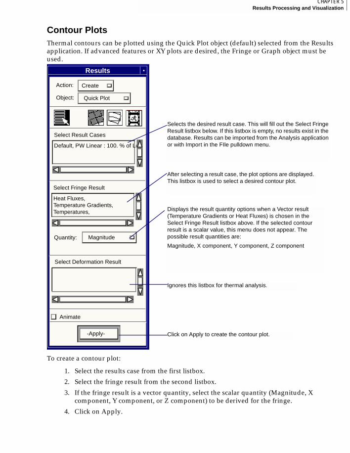
131CHAPTER 5Results Processing and Visualization
5
Contour PlotsThermal contours can be plotted using the Quick Plot object (default) selected from the Results application. If advanced features or XY plots are desired, the Fringe or Graph object must be used.
To create a contour plot:
1. Select the results case from the first listbox.
2. Select the fringe result from the second listbox.
3. If the fringe result is a vector quantity, select the scalar quantity (Magnitude, X component, Y component, or Z component) to be derived for the fringe.
4. Click on Apply.
Results
Default, PW Linear : 100. % of Loa
Select Result Cases
Heat Fluxes,Temperature Gradients,
Select Fringe Result
Quantity:
Select Deformation Result
-Apply-
Temperatures,
Animate
Action: Create
Object: Quick Plot
Magnitude
After selecting a result case, the plot options are displayed. This listbox is used to select a desired contour plot.
Displays the result quantity options when a Vector result (Temperature Gradients or Heat Fluxes) is chosen in the Select Fringe Result listbox above. If the selected contour result is a scalar value, this menu does not appear. The possible result quantities are:
Magnitude, X component, Y component, Z component
Ignores this listbox for thermal analysis.
Selects the desired result case. This will fill out the Select Fringe Result listbox below. If this listbox is empty, no results exist in the database. Results can be imported from the Analysis application or with Import in the FIle pulldown menu.
Click on Apply to create the contour plot.
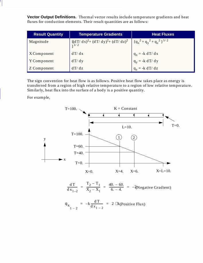
5
132
Vector Output Definitions. Thermal vector results include temperature gradients and heat fluxes for conduction elements. Their result quantities are as follows:
The sign convention for heat flow is as follows. Positive heat flow takes place as energy is transferred from a region of high relative temperature to a region of low relative temperature. Similarly, heat flux into the surface of a body is a positive quantity.
For example,
Result Quantity Temperature Gradients Heat Fluxes
Magnitude {(dT/dx)2+ (dT/dy)2+ (dT/dz)2
} 1/2{ qx
2 + qy2
+ qz2
} 1/2
X Component dT/dx qx = -k dT/dx
Y Component dT/dy qy = -k dT/dy
Z Component dT/dz qz = -k dT/dz
X=L=10.X=6.X=4.X=0.
T=0.
T=40.
T=60.
T=100.
T=100.
T=0.L=10.
K = Constant
dTdx1 2–---------------
T2 T1–
X2 X1–--------------------- 40. 60.–
6. 4.–---------------------- 2.–= = = (Negative Gradient)
qx1 2–
k dTdx1 2–------------------– 2 k⋅= = (Positive Flux)
y
x
1 2
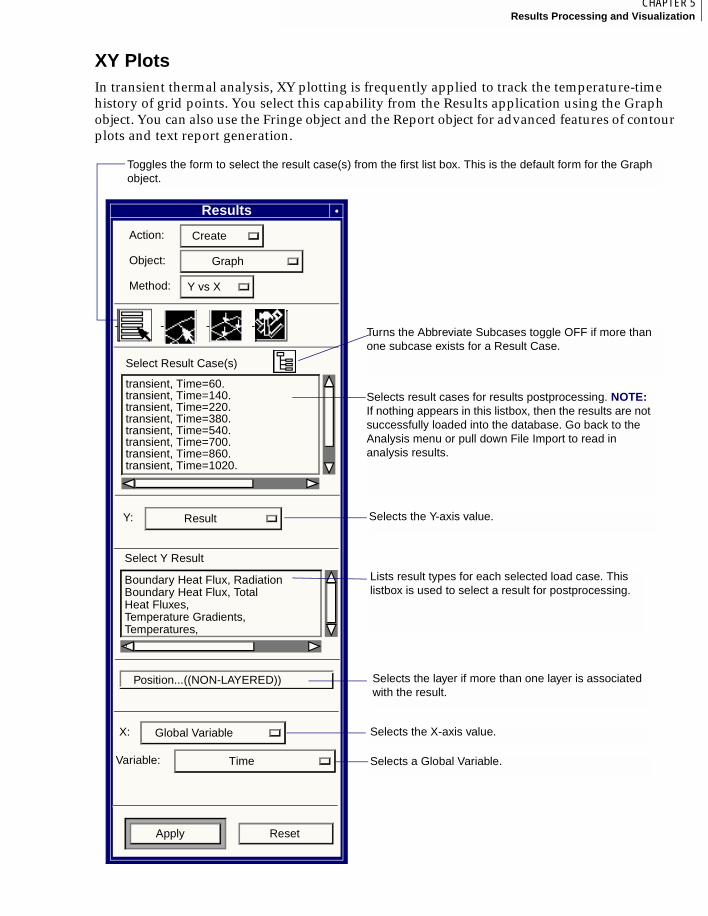
133CHAPTER 5Results Processing and Visualization
5
XY PlotsIn transient thermal analysis, XY plotting is frequently applied to track the temperature-time history of grid points. You select this capability from the Results application using the Graph object. You can also use the Fringe object and the Report object for advanced features of contour plots and text report generation.
Selects result cases for results postprocessing. NOTE: If nothing appears in this listbox, then the results are not successfully loaded into the database. Go back to the Analysis menu or pull down File Import to read in analysis results.
Toggles the form to select the result case(s) from the first list box. This is the default form for the Graph object.
Turns the Abbreviate Subcases toggle OFF if more than one subcase exists for a Result Case.
Results Display
Lists result types for each selected load case. This listbox is used to select a result for postprocessing.
Results
Action: Create
Object: Graph
Method: Y vs X
-none- -none- -none--none-
Apply Reset
Select Result Case(s)
transient, Time=60.transient, Time=140.transient, Time=220.transient, Time=380.transient, Time=540.transient, Time=700.transient, Time=860.transient, Time=1020.
Select Y Result
Boundary Heat Flux, RadiationBoundary Heat Flux, TotalHeat Fluxes,Temperature Gradients,Temperatures,,
Position...((NON-LAYERED))
Y: Result
X: Global Variable
Variable: Time
Selects the Y-axis value.
Selects the X-axis value.
Selects a Global Variable.
Selects the layer if more than one layer is associated with the result.
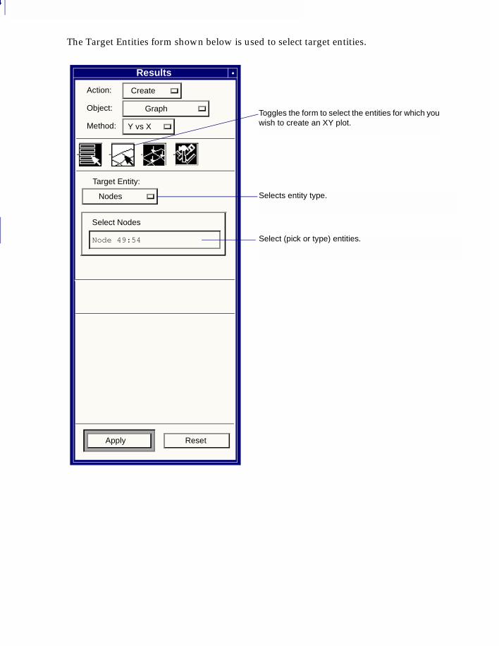
5
134
The Target Entities form shown below is used to select target entities.
Select (pick or type) entities.
Selects entity type.
Results
Action: Create
Object: Graph
Method: Y vs X
-none- -none- -none--none-
Apply Reset
Target Entity:
Nodes
Select Nodes
Node 49:54
Toggles the form to select the entities for which you wish to create an XY plot.
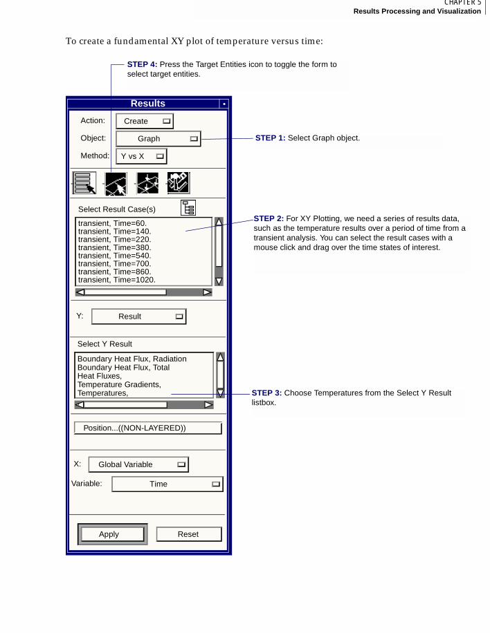
135CHAPTER 5Results Processing and Visualization
5
To create a fundamental XY plot of temperature versus time:
STEP 4: Press the Target Entities icon to toggle the form to select target entities.
STEP 3: Choose Temperatures from the Select Y Result listbox.
STEP 1: Select Graph object.
STEP 2: For XY Plotting, we need a series of results data, such as the temperature results over a period of time from a transient analysis. You can select the result cases with a mouse click and drag over the time states of interest.
Results
Action: Create
Object: Graph
Method: Y vs X
-none- -none- -none--none-
Apply Reset
Select Result Case(s)
transient, Time=60.transient, Time=140.transient, Time=220.transient, Time=380.transient, Time=540.transient, Time=700.transient, Time=860.transient, Time=1020.
Select Y Result
Boundary Heat Flux, RadiationBoundary Heat Flux, TotalHeat Fluxes,Temperature Gradients,Temperatures,,
Position...((NON-LAYERED))
Y: Result
X: Global Variable
Variable: Time
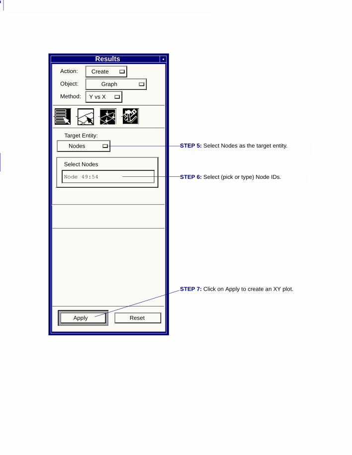
5
136
STEP 5: Select Nodes as the target entity.
STEP 6: Select (pick or type) Node IDs.
STEP 7: Click on Apply to create an XY plot.
Results
Action: Create
Object: Graph
Method: Y vs X
-none- -none- -none--none-
Apply Reset
Target Entity:
Nodes
Select Nodes
Node 49:54
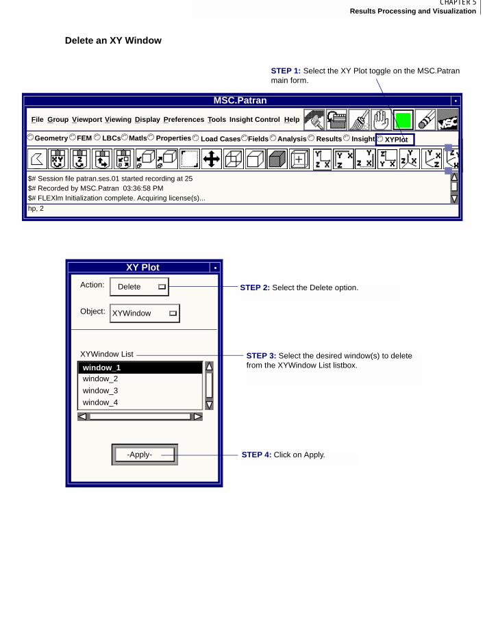
137CHAPTER 5Results Processing and Visualization
5
Delete an XY Window
MSC.Patran
hp, 2
$# Session file patran.ses.01 started recording at 25$# Recorded by MSC.Patran 03:36:58 PM$# FLEXlm Initialization complete. Acquiring license(s)...
File Group Viewport Display Preferences Tools HelpInsight Control
Geometry© FEM LBCs Matls Properties© ©© © Load Cases© Fields Analysis Results Insight© ©© © XYPlot©
Viewing
STEP 1: Select the XY Plot toggle on the MSC.Patran main form.
XY Plot
Action: Delete
Object: XYWindow
-Apply-
XYWindow List
window_2
window_3
window_4
window_1
STEP 3: Select the desired window(s) to delete from the XYWindow List listbox.
STEP 2: Select the Delete option.
STEP 4: Click on Apply.

5
138

MSC.Patran MSC.Nastran Preference Guide, Volume 2: Thermal Analysis
CHAPTER
6 Read Input File
■ Review of Read Input File Form
■ Data Translated from the NASTRAN Input File
■ Conflict Resolution
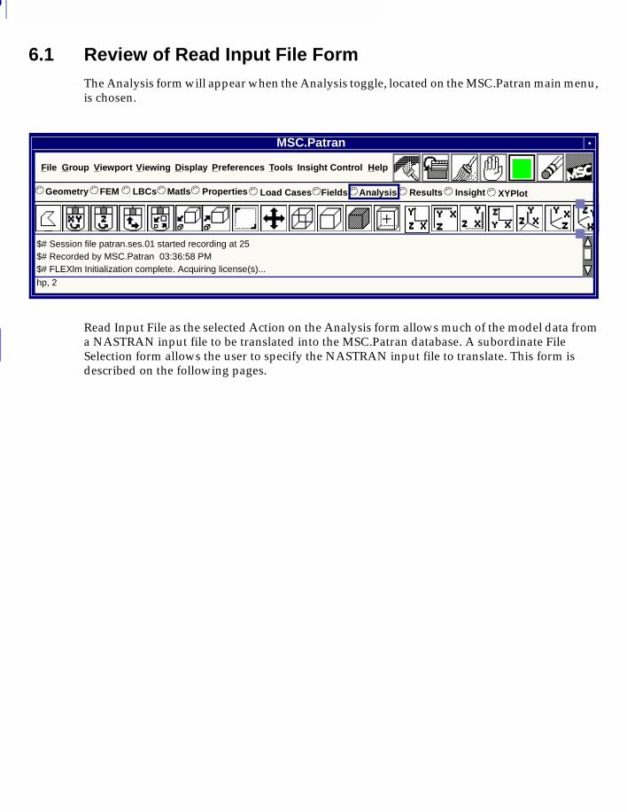
6
140
6.1 Review of Read Input File FormThe Analysis form will appear when the Analysis toggle, located on the MSC.Patran main menu, is chosen.
Read Input File as the selected Action on the Analysis form allows much of the model data from a NASTRAN input file to be translated into the MSC.Patran database. A subordinate File Selection form allows the user to specify the NASTRAN input file to translate. This form is described on the following pages.
MSC.Patran
hp, 2
$# Session file patran.ses.01 started recording at 25$# Recorded by MSC.Patran 03:36:58 PM$# FLEXlm Initialization complete. Acquiring license(s)...
File Group Viewport Display Preferences Tools HelpInsight Control
Geometry© FEM LBCs Matls Properties© ©© © Load Cases© Fields Analysis Results Insight© ©© © XYPlot©
Viewing
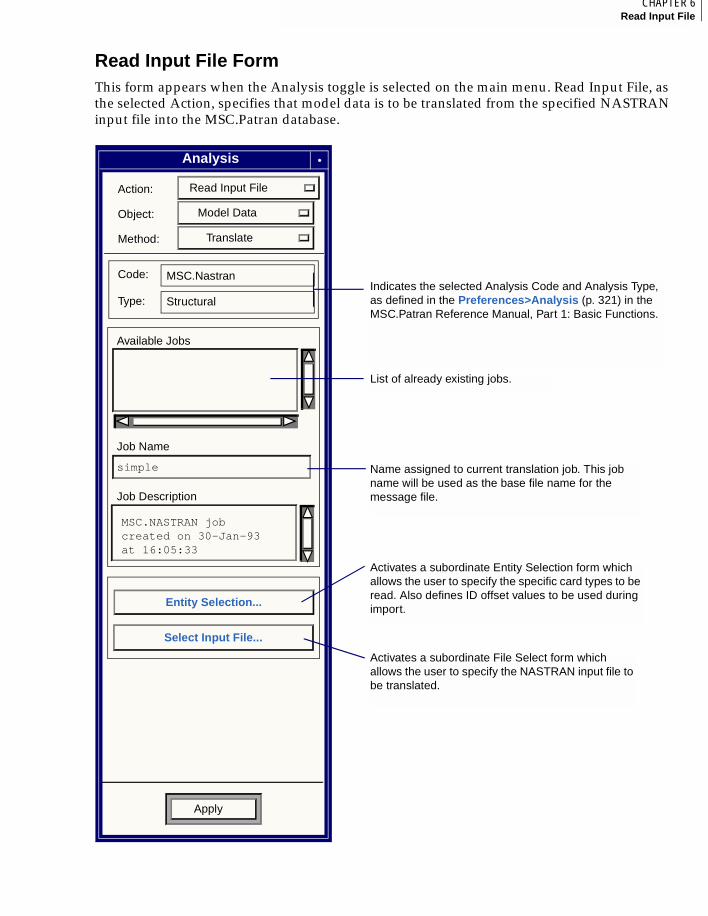
141CHAPTER 6Read Input File
6
Read Input File FormThis form appears when the Analysis toggle is selected on the main menu. Read Input File, as the selected Action, specifies that model data is to be translated from the specified NASTRAN input file into the MSC.Patran database.
Analysis
Read Input File Action:
Model Data Object:
Translate Method:
Code:
Type:
MSC.Nastran
Structural
Available Jobs
Job Name
simple
Job Description
Select Input File...
Apply
MSC.NASTRAN jobcreated on 30-Jan-93at 16:05:33
Entity Selection...
Indicates the selected Analysis Code and Analysis Type, as defined in the Preferences>Analysis (p. 321) in the MSC.Patran Reference Manual, Part 1: Basic Functions.
List of already existing jobs.
Name assigned to current translation job. This job name will be used as the base file name for the message file.
Activates a subordinate File Select form which allows the user to specify the NASTRAN input file to be translated.
Activates a subordinate Entity Selection form which allows the user to specify the specific card types to be read. Also defines ID offset values to be used during import.
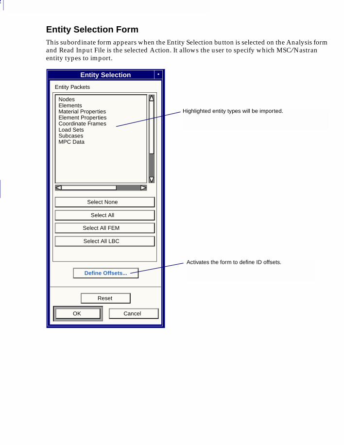
6
142
Entity Selection FormThis subordinate form appears when the Entity Selection button is selected on the Analysis form and Read Input File is the selected Action. It allows the user to specify which MSC ⁄Nastran entity types to import.
Entity Selection
Entity Packets
Nodes Elements Material Properties Element Properties Coordinate Frames Load Sets Subcases MPC Data
Select None
Select All
Select All FEM
Select All LBC
Define Offsets...
Reset
OK Cancel
Highlighted entity types will be imported.
Activates the form to define ID offsets.
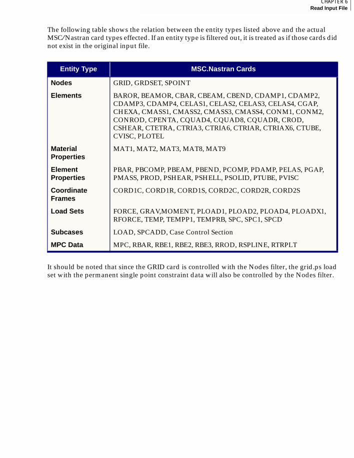
143CHAPTER 6Read Input File
6
The following table shows the relation between the entity types listed above and the actual MSC ⁄Nastran card types effected. If an entity type is filtered out, it is treated as if those cards did not exist in the original input file.
It should be noted that since the GRID card is controlled with the Nodes filter, the grid.ps load set with the permanent single point constraint data will also be controlled by the Nodes filter.
Entity Type MSC.Nastran Cards
Nodes GRID, GRDSET, SPOINT
Elements BAROR, BEAMOR, CBAR, CBEAM, CBEND, CDAMP1, CDAMP2, CDAMP3, CDAMP4, CELAS1, CELAS2, CELAS3, CELAS4, CGAP, CHEXA, CMASS1, CMASS2, CMASS3, CMASS4, CONM1, CONM2, CONROD, CPENTA, CQUAD4, CQUAD8, CQUADR, CROD, CSHEAR, CTETRA, CTRIA3, CTRIA6, CTRIAR, CTRIAX6, CTUBE, CVISC, PLOTEL
Material Properties
MAT1, MAT2, MAT3, MAT8, MAT9
Element Properties
PBAR, PBCOMP, PBEAM, PBEND, PCOMP, PDAMP, PELAS, PGAP, PMASS, PROD, PSHEAR, PSHELL, PSOLID, PTUBE, PVISC
Coordinate Frames
CORD1C, CORD1R, CORD1S, CORD2C, CORD2R, CORD2S
Load Sets FORCE, GRAV,MOMENT, PLOAD1, PLOAD2, PLOAD4, PLOADX1, RFORCE, TEMP, TEMPP1, TEMPRB, SPC, SPC1, SPCD
Subcases LOAD, SPCADD, Case Control Section
MPC Data MPC, RBAR, RBE1, RBE2, RBE3, RROD, RSPLINE, RTRPLT
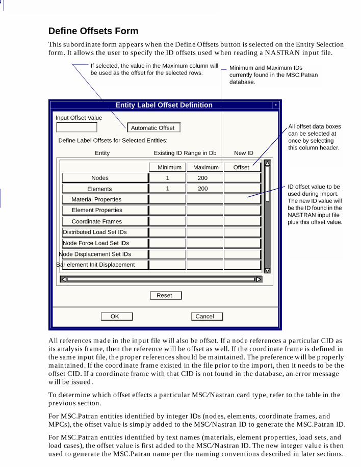
6
144
Define Offsets FormThis subordinate form appears when the Define Offsets button is selected on the Entity Selection form. It allows the user to specify the ID offsets used when reading a NASTRAN input file.
All references made in the input file will also be offset. If a node references a particular CID as its analysis frame, then the reference will be offset as well. If the coordinate frame is defined in the same input file, the proper references should be maintained. The preference will be properly maintained. If the coordinate frame existed in the file prior to the import, then it needs to be the offset CID. If a coordinate frame with that CID is not found in the database, an error message will be issued.
To determine which offset effects a particular MSC ⁄Nastran card type, refer to the table in the previous section.
For MSC.Patran entities identified by integer IDs (nodes, elements, coordinate frames, and MPCs), the offset value is simply added to the MSC ⁄Nastran ID to generate the MSC.Patran ID.
For MSC.Patran entities identified by text names (materials, element properties, load sets, and load cases), the offset value is first added to the MSC ⁄Nastran ID. The new integer value is then used to generate the MSC.Patran name per the naming conventions described in later sections.
Entity Label Offset Definition
Input Offset Value
Define Label Offsets for Selected Entities:
Entity
Minimum Maximum Offset
Reset
Cancel OK
Nodes
Elements
Material Properties
Element Properties
Coordinate Frames
Distributed Load Set IDs
Node Force Load Set IDs
Node Displacement Set IDs
Bar element Init Displacement
1
1
200
200
Automatic Offset
Existing ID Range in Db New ID
Minimum and Maximum IDs currently found in the MSC.Patran database.
ID offset value to be used during import. The new ID value will be the ID found in the NASTRAN input file plus this offset value.
If selected, the value in the Maximum column will be used as the offset for the selected rows.
All offset data boxes can be selected at once by selecting this column header.
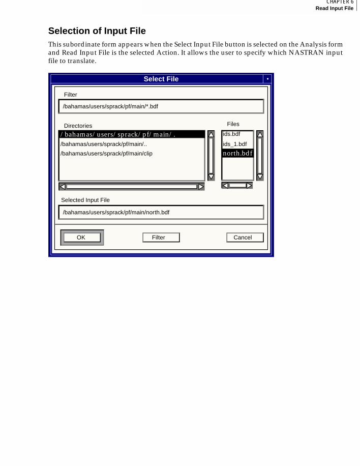
145CHAPTER 6Read Input File
6
Selection of Input FileThis subordinate form appears when the Select Input File button is selected on the Analysis form and Read Input File is the selected Action. It allows the user to specify which NASTRAN input file to translate.
Select File
OK Filter Cancel
Filter
Selected Input File
Directories Files
/bahamas/users/sprack/pf/main/. /bahamas/users/sprack/pf/main/..
/bahamas/users/sprack/pf/main/clip
/bahamas/users/sprack/pf/main/*.bdf
/bahamas/users/sprack/pf/main/north.bdf
ids.bdf
ids_1.bdf
north.bdf
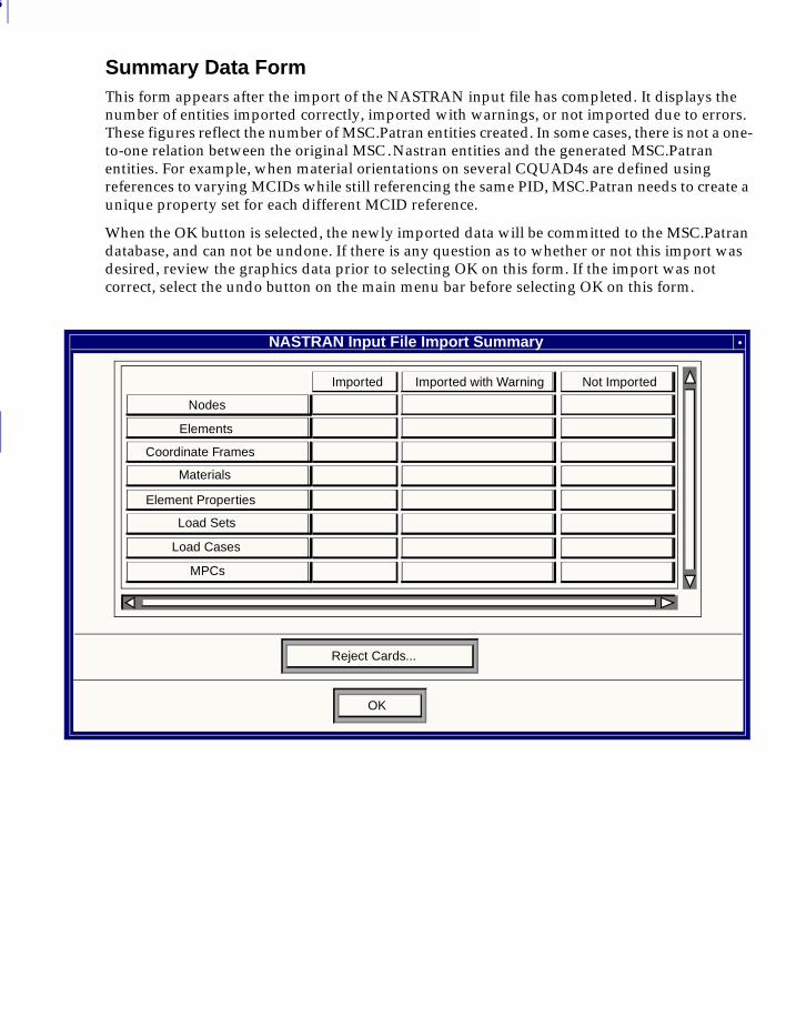
6
146
Summary Data FormThis form appears after the import of the NASTRAN input file has completed. It displays the number of entities imported correctly, imported with warnings, or not imported due to errors. These figures reflect the number of MSC.Patran entities created. In some cases, there is not a one-to-one relation between the original MSC.Nastran entities and the generated MSC.Patran entities. For example, when material orientations on several CQUAD4s are defined using references to varying MCIDs while still referencing the same PID, MSC.Patran needs to create a unique property set for each different MCID reference.
When the OK button is selected, the newly imported data will be committed to the MSC.Patran database, and can not be undone. If there is any question as to whether or not this import was desired, review the graphics data prior to selecting OK on this form. If the import was not correct, select the undo button on the main menu bar before selecting OK on this form.
NASTRAN Input File Import Summary
Reject Cards...
OK
Imported Imported with Warning Not Imported
Nodes
Elements
Coordinate Frames
Materials
Element Properties
Load Sets
Load Cases
MPCs
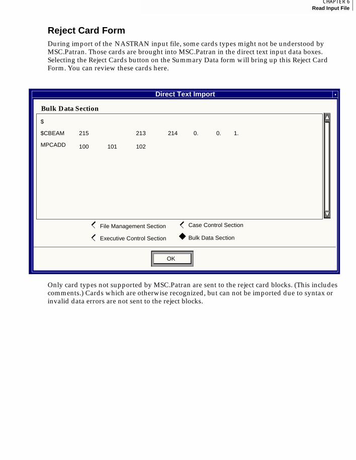
147CHAPTER 6Read Input File
6
Reject Card FormDuring import of the NASTRAN input file, some cards types might not be understood by MSC.Patran. Those cards are brought into MSC.Patran in the direct text input data boxes. Selecting the Reject Cards button on the Summary Data form will bring up this Reject Card Form. You can review these cards here.
Only card types not supported by MSC.Patran are sent to the reject card blocks. (This includes comments.) Cards which are otherwise recognized, but can not be imported due to syntax or invalid data errors are not sent to the reject blocks.
Direct Text Import
OK
Executive Control Section Bulk Data Section
0.
File Management Section Case Control Section
214
Bulk Data Section
215
101
$
1.213$CBEAM
MPCADD 100 102
0.
◆
◆◆
◆◆
◆◆

6
148
6.2 Data Translated from the NASTRAN Input FileFor more information about which specific MSC.Nastran card types can currently be read into MSC.Patran, see Data Translated from the NASTRAN Input File (p. 320) in the MSC.Patran MSC.Nastran Preference Guide, Volume 1: Structural Analysis.

149CHAPTER 6Read Input File
6
6.3 Conflict ResolutionIf an entity can not be imported into MSC.Patran because another entity already exists with that ID or name, then the conflict resolution logic is used. For more information, see Conflict Resolution (p. 332) in the MSC.Patran MSC.Nastran Preference Guide, Volume 1: Structural Analysis.

6
150
MSC.Patran MSC.Nastran Preference Guide, Volume 2: Thermal Analysis
CHAPTER
7 Example Problems
■ Overview
■ Example 1 - Transient Thermal Analysis
■ Example 2 - Free Convection on Printed Circuit Board
■ Example 3 - Forced Air Convection on Printed Circuit Board
■ Example 4 - Thermal Contact Resistance
■ Example 5 - Typical Avionics Flow
■ Example 6 - Radiation Enclosures
■ Example 7 - Axisymmetric Flow in a Pipe
■ Example 8 - Directional Heat Loads
■ Example 9 - Thermal Stress Analysis from Directional Heat Loads
■ Example 10 - Thermal Stress Analysis of a Bi-Metallic Plate
7
152
7.1 OverviewThis chapter provides ten examples that illustrate popular capabilities in MSC.Patran’s interface to the MSC.Nastran thermal solver. The first example, which describes transient thermal analysis, is an extension of the steady state modeling exercise given in Getting Started - A Guided Exercise (Ch. 2). This example contains step-by-step descriptions of the menu picks involved in the modeling process.
Examples 2 through 10 are in easy to follow tutorial format. The actual menu structures are not shown since the expectation is for the user to follow along interactively with the MSC.Patran modeling system.
The session files of the example problems described in this chapter are delivered with the software. To run an example problem:
1. Start MSC/PATRAN by entering the command p3.
1. From MSC/PATRAN’s main form, pull down the File menu and select Session -- Play. A Play Session File form will appear.
1. Select nastherm_exn.ses from the Session File List listbox.
1. Click on Apply.
MSC/PATRAN will execute the modeling process and show you how to build the model.
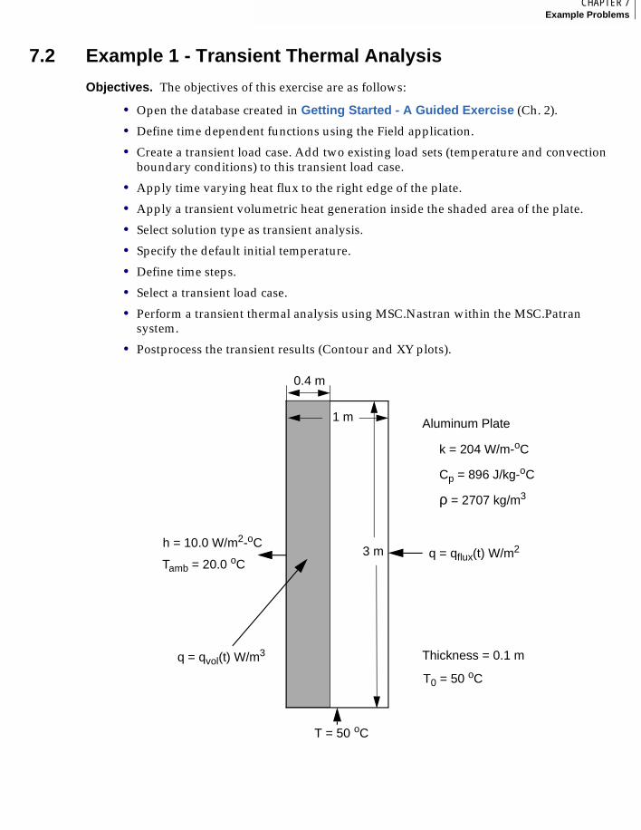
153CHAPTER 7Example Problems
7
7.2 Example 1 - Transient Thermal Analysis
Objectives. The objectives of this exercise are as follows:
• Open the database created in Getting Started - A Guided Exercise (Ch. 2).
• Define time dependent functions using the Field application.
• Create a transient load case. Add two existing load sets (temperature and convection boundary conditions) to this transient load case.
• Apply time varying heat flux to the right edge of the plate.
• Apply a transient volumetric heat generation inside the shaded area of the plate.
• Select solution type as transient analysis.
• Specify the default initial temperature.
• Define time steps.
• Select a transient load case.
• Perform a transient thermal analysis using MSC.Nastran within the MSC.Patran system.
• Postprocess the transient results (Contour and XY plots).
3 m
Aluminum Plate
k = 204 W/m-oC
Cp = 896 J/kg-oC
ρ = 2707 kg/m3
q = qflux(t) W/m2
T = 50 oC
Tamb = 20.0 oC
h = 10.0 W/m2-oC
Thickness = 0.1 m
1 m
q = qvol(t) W/m3
0.4 m
T0 = 50 oC
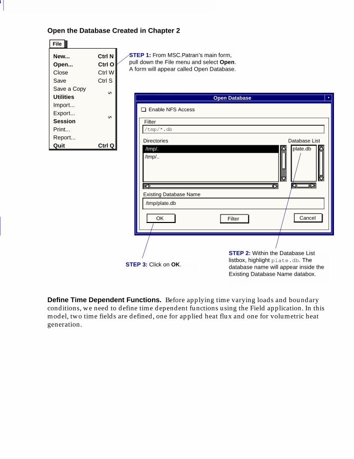
7
154
Open the Database Created in Chapter 2
Define Time Dependent Functions. Before applying time varying loads and boundary conditions, we need to define time dependent functions using the Field application. In this model, two time fields are defined, one for applied heat flux and one for volumetric heat generation.
File
New... Ctrl NOpen... Ctrl OClose Ctrl WSave Ctrl SSave a Copy UtilitiesImport... Export...SessionPrint... Report...Quit Ctrl Q
ss
New Database Name
Apply Filter Cancel
Open Database
/tmp/*.db
Filter
/tmp/..
/tmp/.
Directories Database List
OK
Existing Database Name
Cancel Filter
Enable NFS Access
plate.db
/tmp/plate.db
STEP 1: From MSC.Patran’s main form, pull down the File menu and select Open. A form will appear called Open Database.
STEP 2: Within the Database List listbox, highlight plate.db. The database name will appear inside the Existing Database Name databox.
STEP 3: Click on OK.
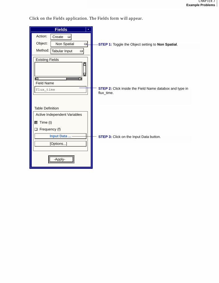
155CHAPTER 7Example Problems
7
Click on the Fields application. The Fields form will appear.
Fields
Action: Create
Object: Non Spatial
Method: Tabular Input
Existing Fields
Field Name
flux_time
Table Definition
Active Independent Variables
Time (t)
Frequency (f)
Input Data ...
[Options...]
-Apply-
STEP 1: Toggle the Object setting to Non Spatial.
STEP 2: Click inside the Field Name databox and type in flux_time.
STEP 3: Click on the Input Data button.
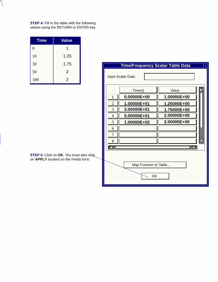
7
156
Time/Frequency Scalar Table Data
Input Scalar Data
Map Function to Table...
OK
3
54
21
7
8
6
Time(t) Value
0.00000E+00
1.00000E+013.00000E+01
5.00000E+01
1.00000E+02
1.00000E+00
1.25000E+001.75000E+002.00000E+00
2.00000E+00
STEP 5: Click on OK. You must also click on APPLY located on the Fields form.
STEP 4: Fill in the table with the following values using the RETURN or ENTER key.
Time Value
0 1
10 1.25
30 1.75
50 2
100 2
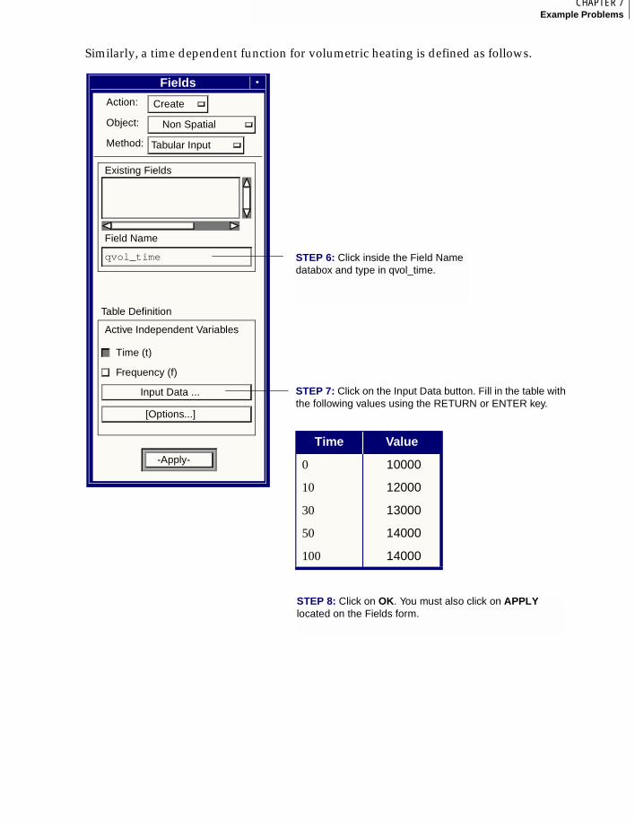
157CHAPTER 7Example Problems
7
Similarly, a time dependent function for volumetric heating is defined as follows.
STEP 7: Click on the Input Data button. Fill in the table with the following values using the RETURN or ENTER key.
Time Value
0 10000
10 12000
30 13000
50 14000
100 14000
Fields
Action: Create
Object: Non Spatial
Method: Tabular Input
Existing Fields
Field Name
qvol_time
Table Definition
Active Independent Variables
Time (t)
Frequency (f)
Input Data ...
[Options...]
-Apply-
STEP 6: Click inside the Field Name databox and type in qvol_time.
STEP 8: Click on OK. You must also click on APPLY located on the Fields form.
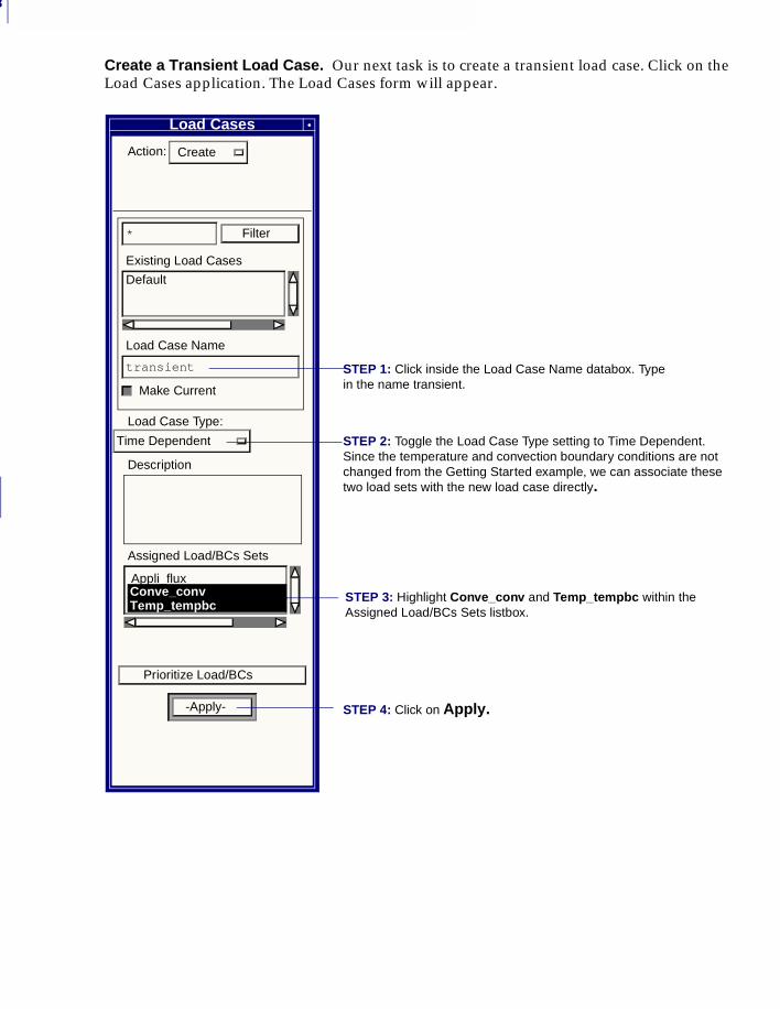
7
158
Create a Transient Load Case. Our next task is to create a transient load case. Click on the Load Cases application. The Load Cases form will appear.
Load Cases
Action: Create
* Filter
Existing Load Cases
Default
Load Case Name
transient
Make Current
Load Case Type:
Time Dependent
Description
Assigned Load/BCs Sets
Prioritize Load/BCs
-Apply-
Appli_fluxConve_convTemp _tempbc
STEP 4: Click on Apply.
Conve_convTemp_tempbc
STEP 1: Click inside the Load Case Name databox. Type in the name transient.
STEP 2: Toggle the Load Case Type setting to Time Dependent. Since the temperature and convection boundary conditions are not changed from the Getting Started example, we can associate these two load sets with the new load case directly.
STEP 3: Highlight Conve_conv and Temp_tempbc within the Assigned Load/BCs Sets listbox.
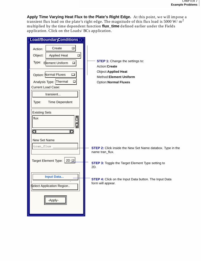
159CHAPTER 7Example Problems
7
Apply Time Varying Heat Flux to the Plate’s Right Edge. At this point, we will impose a transient flux load on the plate’s right edge. The magnitude of this flux load is 5000 W/m2 multiplied by the time dependent function flux_time defined earlier under the Fields application. Click on the Loads/BCs application.
Load/Boundary Conditions
Create Action:
Thermal Analysis Type:
Applied HeatObject:
Element UniformType:
transient...
Type: Time Dependent
Current Load Case:
Existing Sets
flux
tran_flux
New Set Name
Input Data...
Select Application Region..
.
-Apply-
Normal FluxesOption:
Target Element Type: 2D
STEP 1: Change the settings to:
Action:Create
Object:Applied Heat
Method:Element Uniform
Option:Normal Fluxes
STEP 4: Click on the Input Data button. The Input Data form will appear.
STEP 2: Click inside the New Set Name databox. Type in the name tran_flux.
STEP 3: Toggle the Target Element Type setting to 2D.
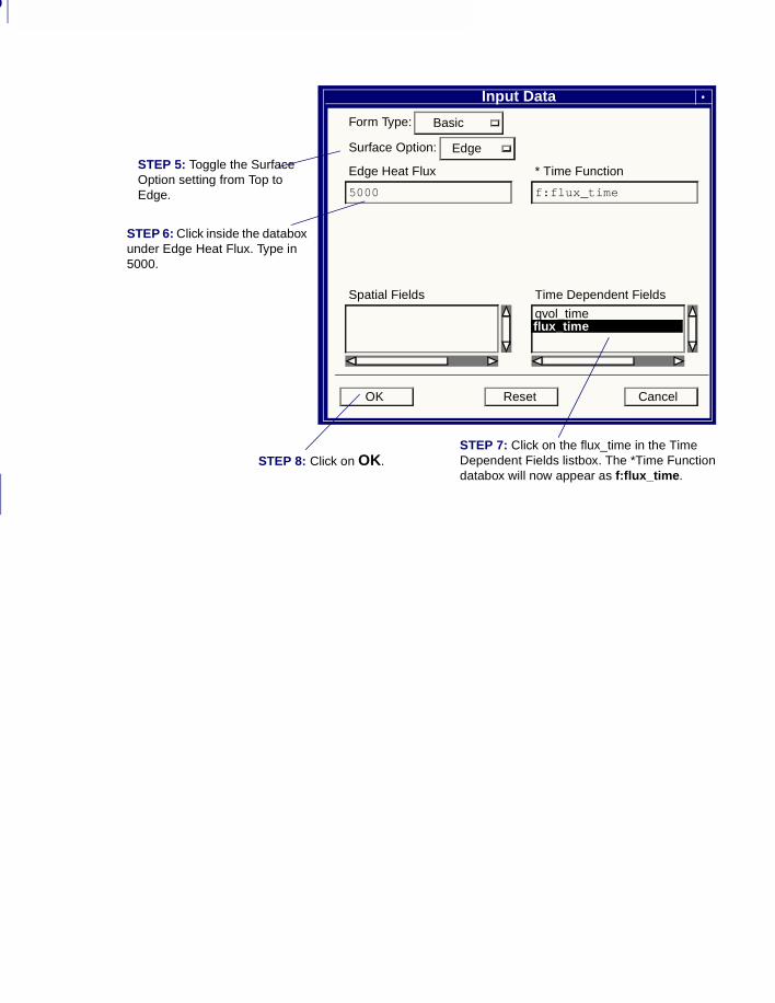
7
160
Input Data
Form Type: Basic
Surface Option: Edge
Edge Heat Flux
5000
* Time Function
f:flux_time
Spatial Fields Time Dependent Fields
qvol_timeflux_time
ResetOK Cancel
flux_time
STEP 5: Toggle the Surface Option setting from Top to Edge.
STEP 6: Click inside the databox under Edge Heat Flux. Type in 5000.
STEP 7: Click on the flux_time in the Time Dependent Fields listbox. The *Time Function databox will now appear as f:flux_time.
STEP 8: Click on OK.
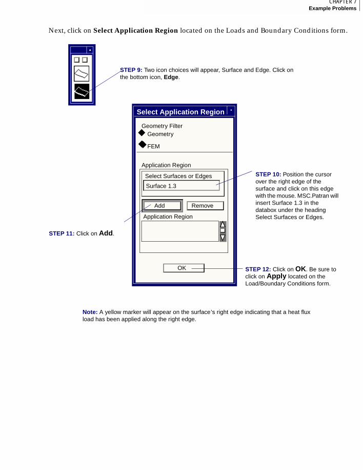
161CHAPTER 7Example Problems
7
Next, click on Select Application Region located on the Loads and Boundary Conditions form.
Geometry
FEM
Geometry Filter
Select Surfaces or Edges
Add Remove
Application Region
Application Region
OK
◆
◆◆
Select Application Region
Surface 1.3
STEP 9: Two icon choices will appear, Surface and Edge. Click on the bottom icon, Edge.
STEP 10: Position the cursor over the right edge of the surface and click on this edge with the mouse. MSC.Patran will insert Surface 1.3 in the databox under the heading Select Surfaces or Edges.
STEP 12: Click on OK. Be sure to click on Apply located on the Load/Boundary Conditions form.
STEP 11: Click on Add.
Note: A yellow marker will appear on the surface’s right edge indicating that a heat flux load has been applied along the right edge.
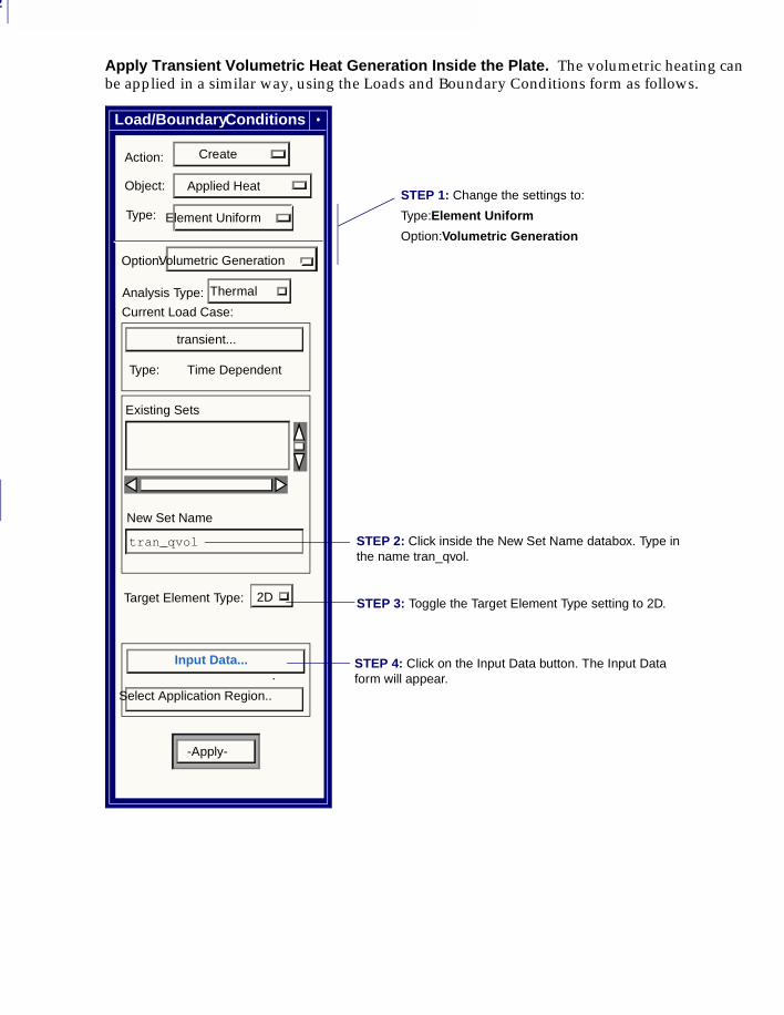
7
162
Apply Transient Volumetric Heat Generation Inside the Plate. The volumetric heating can be applied in a similar way, using the Loads and Boundary Conditions form as follows.
Load/Boundary Conditions
Create Action:
Thermal Analysis Type:
Applied HeatObject:
Element UniformType:
transient...
Type: Time Dependent
Current Load Case:
Existing Sets
tran_qvol
New Set Name
Input Data...
Select Application Region..
.
-Apply-
Volumetric GenerationOption:
Target Element Type: 2D
STEP 1: Change the settings to:
Type:Element Uniform
Option:Volumetric Generation
STEP 2: Click inside the New Set Name databox. Type in the name tran_qvol.
STEP 3: Toggle the Target Element Type setting to 2D.
STEP 4: Click on the Input Data button. The Input Data form will appear.
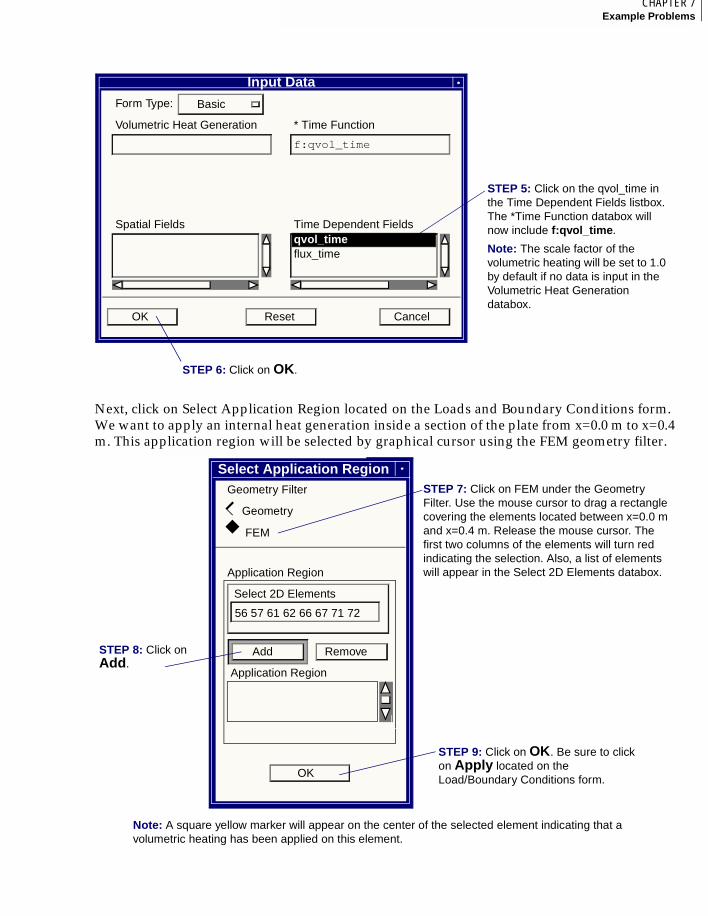
163CHAPTER 7Example Problems
7
Next, click on Select Application Region located on the Loads and Boundary Conditions form. We want to apply an internal heat generation inside a section of the plate from x=0.0 m to x=0.4 m. This application region will be selected by graphical cursor using the FEM geometry filter.
Input DataForm Type: Basic
Volumetric Heat Generation * Time Function
f:qvol_time
Spatial Fields Time Dependent Fields
flux_time
ResetOK Cancel
STEP 5: Click on the qvol_time in the Time Dependent Fields listbox. The *Time Function databox will now include f:qvol_time.
Note: The scale factor of the volumetric heating will be set to 1.0 by default if no data is input in the Volumetric Heat Generation databox.
qvol_time
STEP 6: Click on OK.
Load/Boundary Conditions
Create Action:
Thermal Analysis Type:
Temp (Thermal) Object:
Nodal Type:
Default...
Type: Static
Current Load Case:
Existing Sets
tempbc
New Set Name
Geometry
FEM
Geometry Filter
Select 2D Elements
Add Remove
Application Region
Application Region
OK
◆
◆◆
Select Application Region
56 57 61 62 66 67 71 72
STEP 7: Click on FEM under the Geometry Filter. Use the mouse cursor to drag a rectangle covering the elements located between x=0.0 m and x=0.4 m. Release the mouse cursor. The first two columns of the elements will turn red indicating the selection. Also, a list of elements will appear in the Select 2D Elements databox.
STEP 8: Click on Add.
STEP 9: Click on OK. Be sure to click on Apply located on the Load/Boundary Conditions form.
Note: A square yellow marker will appear on the center of the selected element indicating that a volumetric heating has been applied on this element.
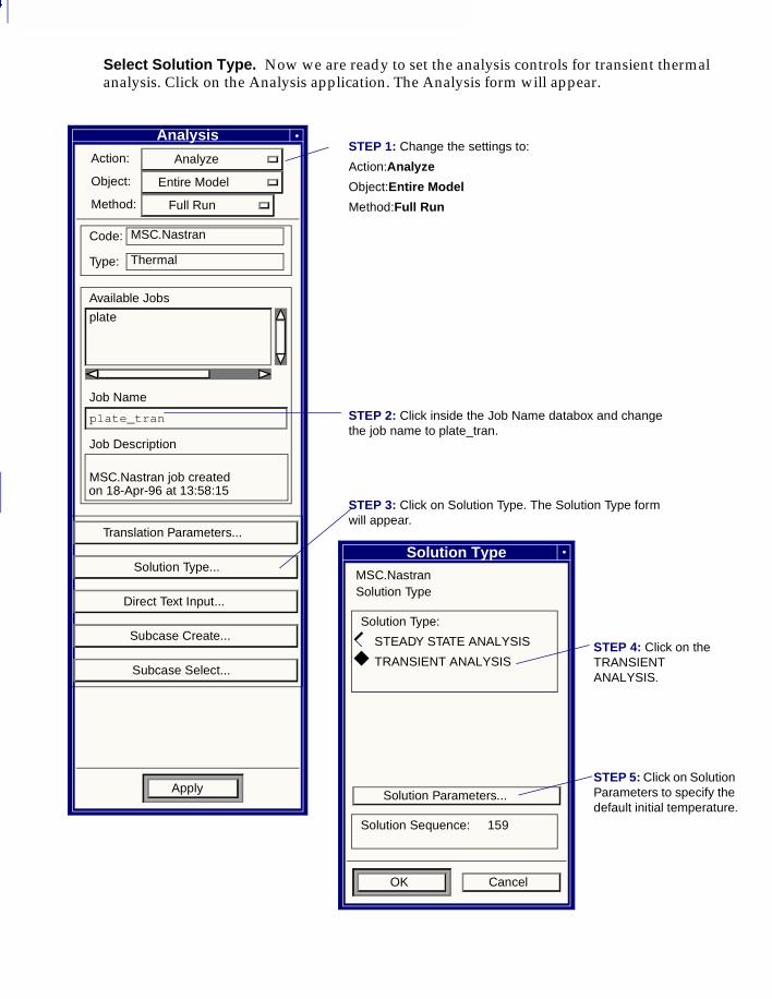
7
164
Select Solution Type. Now we are ready to set the analysis controls for transient thermal analysis. Click on the Analysis application. The Analysis form will appear.
AnalysisAction: Analyze
Object: Entire Model
Method: Full Run
Code:
Type:
MSC.Nastran
Thermal
Available Jobs
plate
Job Name
plate_tran
Job Description
MSC.Nastran job created
Translation Parameters...
Solution Type...
Direct Text Input...
Subcase Create...
Subcase Select...
Apply
on 18-Apr-96 at 13:58:15STEP 3: Click on Solution Type. The Solution Type form will appear.
Solution TypeMSC.NastranSolution Type
Solution Type:
STEADY STATE ANALYSIS
TRANSIENT ANALYSIS
Solution Parameters...
Solution Sequence: 159
OK Cancel
STEP 1: Change the settings to:
Action:Analyze
Object:Entire Model
Method:Full Run
STEP 2: Click inside the Job Name databox and change the job name to plate_tran.
STEP 4: Click on the TRANSIENT ANALYSIS.
STEP 5: Click on Solution Parameters to specify the default initial temperature.
◆◆◆
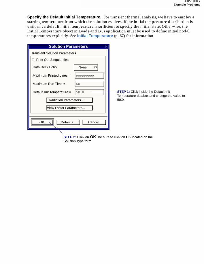
165CHAPTER 7Example Problems
7
Specify the Default Initial Temperature. For transient thermal analysis, we have to employ a starting temperature from which the solution evolves. If the initial temperature distribution is uniform, a default initial temperature is sufficient to specify the initial state. Otherwise, the Initial Temperature object in Loads and BCs application must be used to define initial nodal temperatures explicitly. See Initial Temperature (p. 67) for information.
Solution Parameters
Transient Solution Parameters
Print Out Singularities
Data Deck Echo: None
Maximum Printed Lines = 999999999
Maximum Run Time = 60
Default Init Temperature = 50.0
Radiation Parameters...
View Factor Parameters...
OK Defaults Cancel
STEP 1: Click inside the Default Init Temperature databox and change the value to 50.0.
STEP 2: Click on OK. Be sure to click on OK located on the Solution Type form.
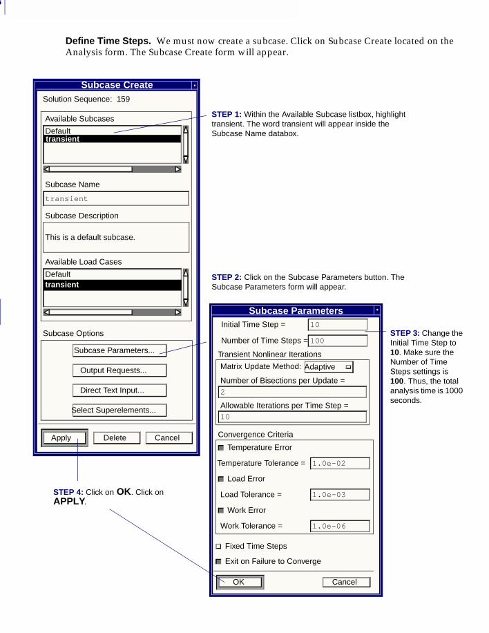
7
166
Define Time Steps. We must now create a subcase. Click on Subcase Create located on the Analysis form. The Subcase Create form will appear.
Subcase CreateSolution Sequence: 159
Available Subcases
Defaulttransient
Subcase Name
transient
Subcase Description
This is a default subcase.
Available Load Cases
Default
Subcase Options
Subcase Parameters...
Output Requests...
Direct Text Input...
Select Superelements...
Apply Delete Cancel
Subcase ParametersInitial Time Step = 10
Number of Time Steps = 100
Transient Nonlinear Iterations
Matrix Update Method: Adaptive
Number of Bisections per Update =2
Allowable Iterations per Time Step =10
Convergence Criteria
Temperature Error
Temperature Tolerance = 1.0e-02
Load Error
Load Tolerance = 1.0e-03
Work Error
Work Tolerance = 1.0e-06
Fixed Time Steps
Exit on Failure to Converge
OK Cancel
STEP 2: Click on the Subcase Parameters button. The Subcase Parameters form will appear.
STEP 3: Change the Initial Time Step to 10. Make sure the Number of Time Steps settings is 100. Thus, the total analysis time is 1000 seconds.
transient
STEP 1: Within the Available Subcase listbox, highlight transient. The word transient will appear inside the Subcase Name databox.
STEP 4: Click on OK. Click on APPLY.
transient
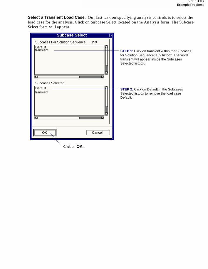
167CHAPTER 7Example Problems
7
Select a Transient Load Case. Our last task on specifying analysis controls is to select the load case for the analysis. Click on Subcase Select located on the Analysis form. The Subcase Select form will appear.
Subcase Select
Subcases For Solution Sequence: 159
Defaulttransient
Subcases Selected:
Default
OK Cancel
Click on OK.
transient
STEP 1: Click on transient within the Subcases for Solution Sequence: 159 listbox. The word transient will appear inside the Subcases Selected listbox.
STEP 2: Click on Default in the Subcases Selected listbox to remove the load case Default.
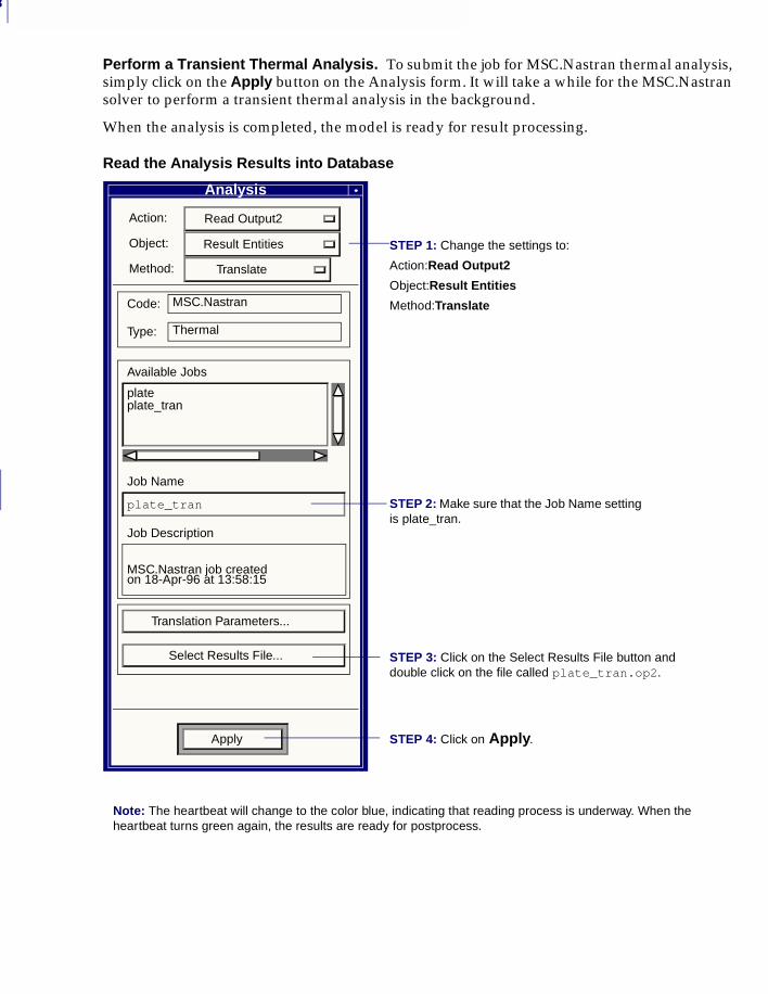
7
168
Perform a Transient Thermal Analysis. To submit the job for MSC.Nastran thermal analysis, simply click on the Apply button on the Analysis form. It will take a while for the MSC.Nastran solver to perform a transient thermal analysis in the background.
When the analysis is completed, the model is ready for result processing.
Read the Analysis Results into Database
Analysis
Action: Read Output2
Object: Result Entities
Method: Translate
Code:
Type:
MSC.Nastran
Thermal
Available Jobs
plate
Job Name
plate_tran
Job Description
MSC.Nastran job created
Translation Parameters...
Select Results File...
Apply
on 18-Apr-96 at 13:58:15
plate_tran
STEP 1: Change the settings to:
Action:Read Output2
Object:Result Entities
Method:Translate
STEP 2: Make sure that the Job Name setting is plate_tran.
STEP 3: Click on the Select Results File button and double click on the file called plate_tran.op2.
STEP 4: Click on Apply.
Note: The heartbeat will change to the color blue, indicating that reading process is underway. When the heartbeat turns green again, the results are ready for postprocess.
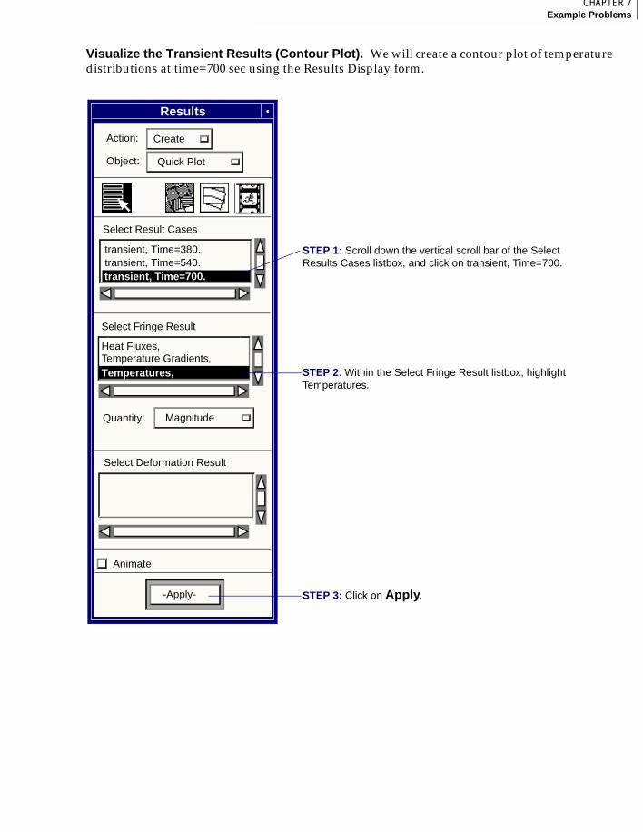
169CHAPTER 7Example Problems
7
Visualize the Transient Results (Contour Plot). We will create a contour plot of temperature distributions at time=700 sec using the Results Display form.
Results Display
STEP 1: Scroll down the vertical scroll bar of the Select Results Cases listbox, and click on transient, Time=700.
STEP 2: Within the Select Fringe Result listbox, highlight Temperatures.
STEP 3: Click on Apply.
Results
Select Result Cases
Heat Fluxes,Temperature Gradients,
Select Fringe Result
Quantity:
Select Deformation Result
-Apply-
Temperatures,
Animate
Action: Create
Object: Quick Plot
Magnitude
transient, Time=380.
transient, Time=700.transient, Time=540.
Temperatures,
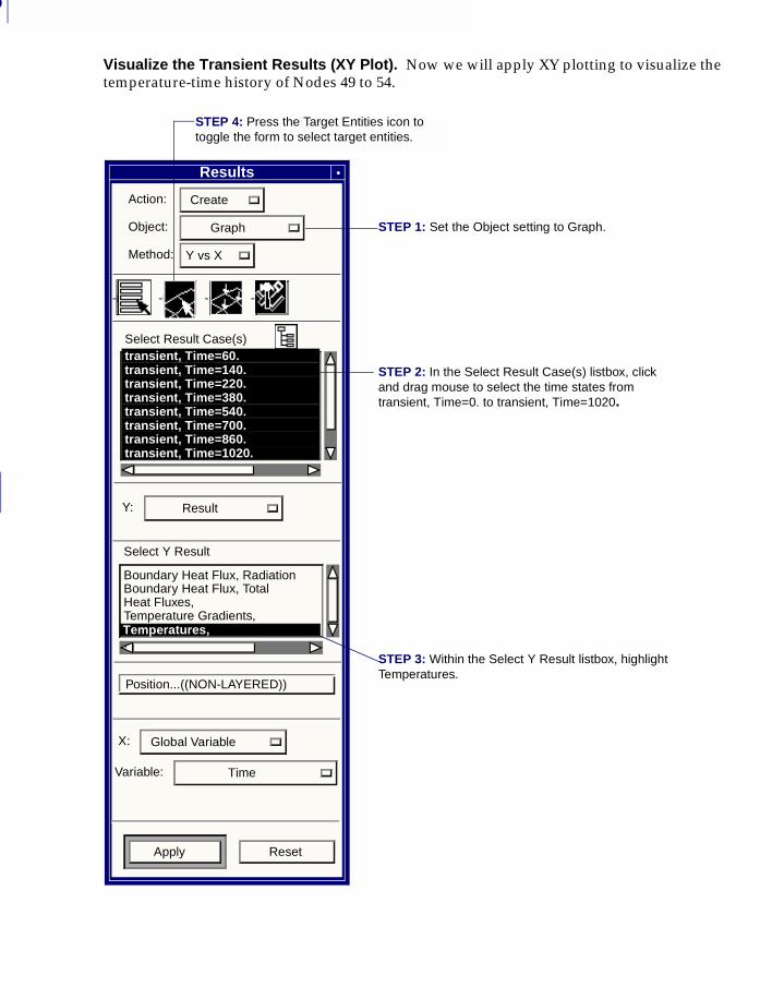
7
170
Visualize the Transient Results (XY Plot). Now we will apply XY plotting to visualize the temperature-time history of Nodes 49 to 54.
STEP 1: Set the Object setting to Graph.
STEP 2: In the Select Result Case(s) listbox, click and drag mouse to select the time states from transient, Time=0. to transient, Time=1020.
STEP 3: Within the Select Y Result listbox, highlight Temperatures.
Results
Action: Create
Object: Graph
Method: Y vs X
-none- -none- -none--none-
Apply Reset
Select Result Case(s)
transient, Time=60.transient, Time=140.transient, Time=220.transient, Time=380.transient, Time=540.transient, Time=700.transient, Time=380.transient, Time=860.
Select Y Result
Boundary Heat Flux, RadiationBoundary Heat Flux, TotalHeat Fluxes,Temperature Gradients,Temperatures,,
Position...((NON-LAYERED))
Y: Result
X: Global Variable
Variable: Time
Temperatures,
transient, Time=60.transient, Time=140.transient, Time=220.transient, Time=380.transient, Time=540.transient, Time=700.transient, Time=860.transient, Time=1020.
STEP 4: Press the Target Entities icon to toggle the form to select target entities.
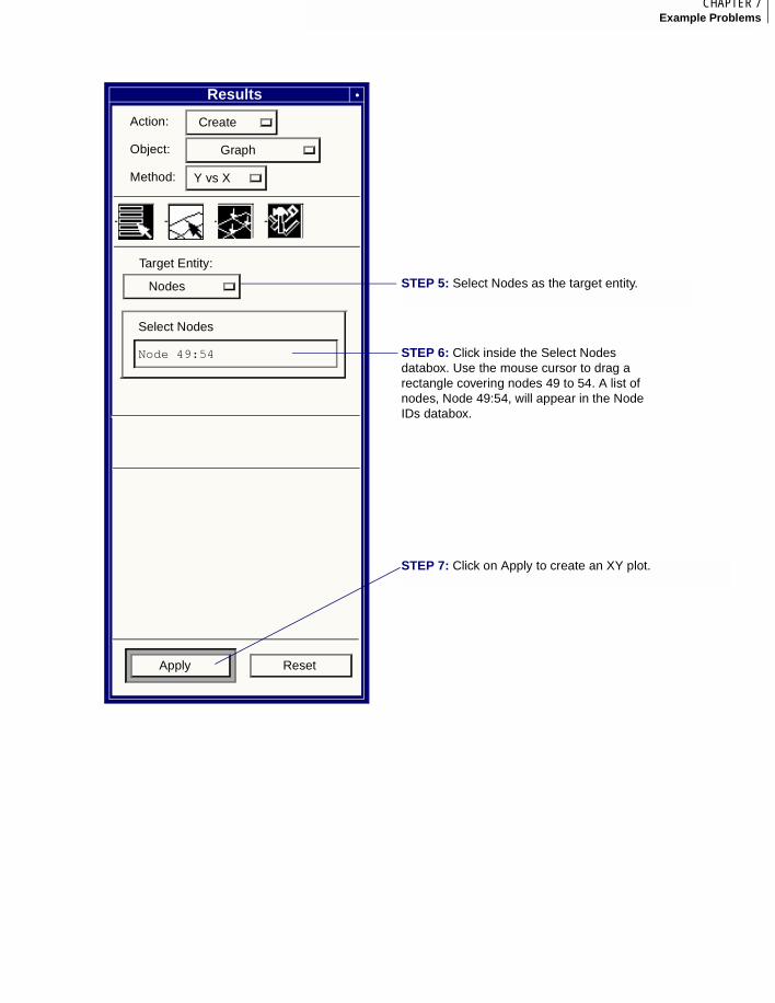
171CHAPTER 7Example Problems
7
STEP 6: Click inside the Select Nodes databox. Use the mouse cursor to drag a rectangle covering nodes 49 to 54. A list of nodes, Node 49:54, will appear in the Node IDs databox.
Results
Action: Create
Object: Graph
Method: Y vs X
-none- -none- -none--none-
Apply Reset
Target Entity:
Nodes
Select Nodes
Node 49:54
STEP 5: Select Nodes as the target entity.
STEP 7: Click on Apply to create an XY plot.
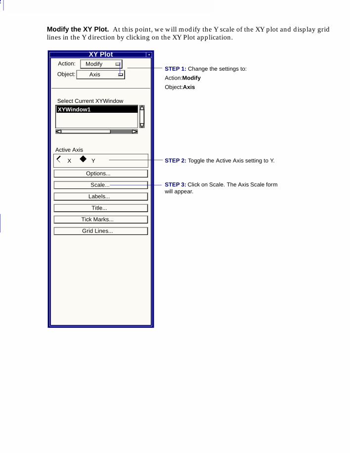
7
172
Modify the XY Plot. At this point, we will modify the Y scale of the XY plot and display grid lines in the Y direction by clicking on the XY Plot application.
XY PlotAction: Modify
Object: Axis
Select Current XYWindowXYWindow1
Active Axis
Options...
Scale...
Labels...
Title...
Tick Marks...
Grid Lines...
XYWindow1
STEP 2: Toggle the Active Axis setting to Y.
STEP 1: Change the settings to:
Action:Modify
Object:Axis
STEP 3: Click on Scale. The Axis Scale form will appear.
◆◆◆ X Y
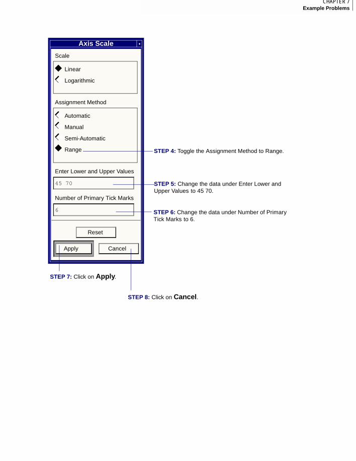
173CHAPTER 7Example Problems
7
Axis Scale
Scale
Linear
Logarithmic
Assignment Method
Automatic
Manual
Semi-Automatic
Range
Enter Lower and Upper Values
45 70
Number of Primary Tick Marks
6
Reset
Apply Cancel
STEP 4: Toggle the Assignment Method to Range.
STEP 5: Change the data under Enter Lower and Upper Values to 45 70.
STEP 6: Change the data under Number of Primary Tick Marks to 6.
STEP 7: Click on Apply.
STEP 8: Click on Cancel.
◆
◆
◆◆
◆◆
◆◆
◆◆
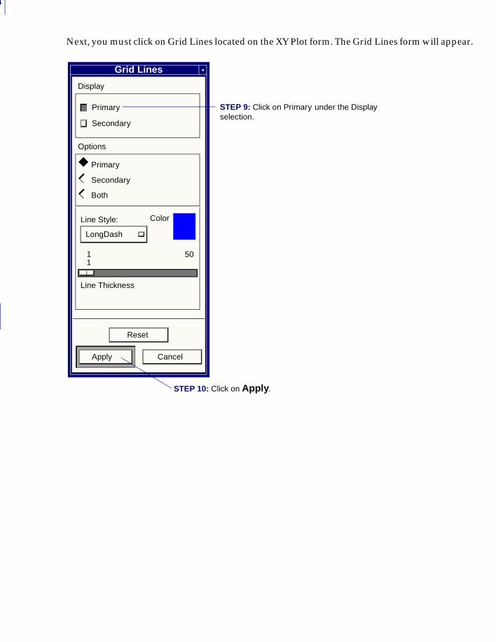
7
174
Next, you must click on Grid Lines located on the XY Plot form. The Grid Lines form will appear.
Grid Lines
Display
Primary
Secondary
Options
Primary
Secondary
Both
Line Style:
LongDash?25
Line Thickness
501
Reset
Apply Cancel
Color
1
STEP 9: Click on Primary under the Display selection.
STEP 10: Click on Apply.
◆
◆◆
◆◆
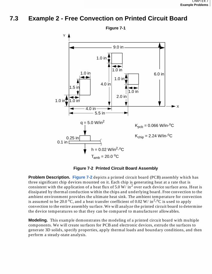
175CHAPTER 7Example Problems
7
7.3 Example 2 - Free Convection on Printed Circuit BoardFigure 7-1
Figure 7-2 Printed Circuit Board Assembly
Problem Description. Figure 7-2 depicts a printed circuit board (PCB) assembly which has three significant chip devices mounted on it. Each chip is generating heat at a rate that is consistent with the application of a heat flux of 5.0 W/in2 over each device surface area. Heat is dissipated by thermal conduction within the chips and underlying board. Free convection to the ambient environment provides the ultimate heat sink. The ambient temperature for convection is assumed to be 20.0 oC, and a heat transfer coefficient of 0.02 W/in2-oC is used to apply convection to the entire assembly surface. We will analyze the printed circuit board to determine the device temperatures so that they can be compared to manufacturer allowables.
Modeling. This example demonstrates the modeling of a printed circuit board with multiple components. We will create surfaces for PCB and electronic devices, extrude the surfaces to generate 3D solids, specify properties, apply thermal loads and boundary conditions, and then perform a steady-state analysis.
q = 5.0 W/in2
Tamb = 20.0 oC
h = 0.02 W/in2-oC
9.0 in
6.0 in1.0 in
1.0 in
1.0 in
1.5 in
0.1 in0.25 in
Kpcb = 0.066 W/in-oC
Kchip = 2.24 W/in-oC
5.5 in4.0 in
1.0 in 1.0 in
4.0 in
1.0 in
1.0 in
2.0 in
X
Y
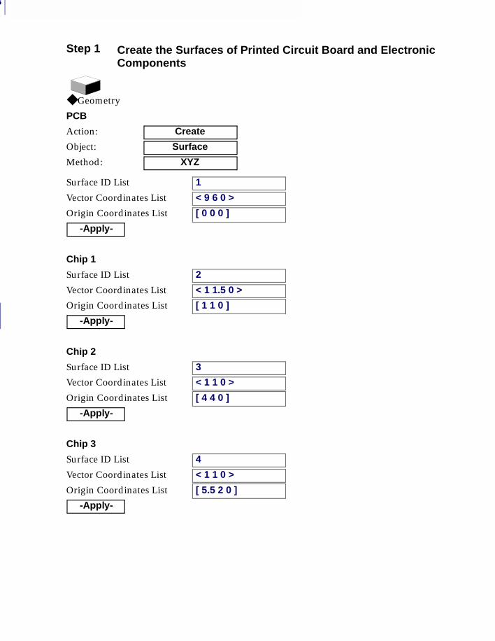
7
176
Step 1 Create the Surfaces of Printed Circuit Board and Electronic Components
◆ Geometry
PCB
Action: Create
Object: Surface
Method: XYZ
Surface ID List 1
Vector Coordinates List < 9 6 0 >
Origin Coordinates List [ 0 0 0 ]
-Apply-
Chip 1
Surface ID List 2
Vector Coordinates List < 1 1.5 0 >
Origin Coordinates List [ 1 1 0 ]
-Apply-
Chip 2
Surface ID List 3
Vector Coordinates List < 1 1 0 >
Origin Coordinates List [ 4 4 0 ]
-Apply-
Chip 3
Surface ID List 4
Vector Coordinates List < 1 1 0 >
Origin Coordinates List [ 5.5 2 0 ]
-Apply-
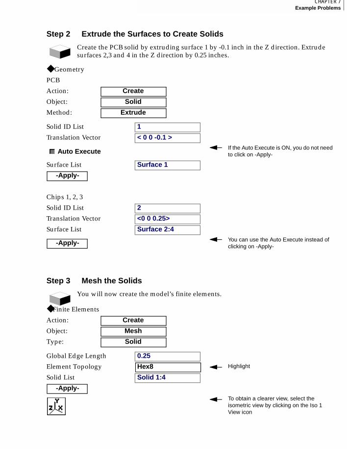
177CHAPTER 7Example Problems
7
Step 2 Extrude the Surfaces to Create Solids
Create the PCB solid by extruding surface 1 by -0.1 inch in the Z direction. Extrude surfaces 2,3 and 4 in the Z direction by 0.25 inches.
◆ Geometry
PCB
Action: Create
Object: Solid
Method: Extrude
Solid ID List 1
Translation Vector < 0 0 -0.1 >
Auto ExecuteIf the Auto Execute is ON, you do not needto click on -Apply-
Surface List Surface 1
-Apply-
Chips 1, 2, 3
Solid ID List 2
Translation Vector <0 0 0.25>
Surface List Surface 2:4
-Apply- You can use the Auto Execute instead of clicking on -Apply-
Step 3 Mesh the Solids
You will now create the model’s finite elements.
◆ Finite Elements
Action: Create
Object: Mesh
Type: Solid
Global Edge Length 0.25
Element Topology Hex8 Highlight
Solid List Solid 1:4
-Apply-To obtain a clearer view, select the isometric view by clicking on the Iso 1 View icon
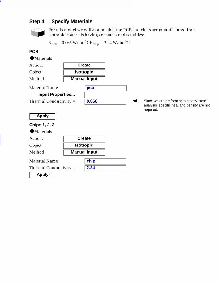
7
178
Step 4 Specify Materials
For this model we will assume that the PCB and chips are manufactured from isotropic materials having constant conductivities:
Kpcb = 0.066 W/in-oCKchip = 2.24 W/in-oC
PCB
◆ Materials
Action: Create
Object: Isotropic
Method: Manual Input
Material Name pcb
Input Properties...
Thermal Conductivity = 0.066 Since we are preforming a steady-state analysis, specific heat and density are notrequired.
-Apply-
Chips 1, 2, 3
◆ Materials
Action: Create
Object: Isotropic
Method: Manual Input
Material Name chip
Thermal Conductivity = 2.24
-Apply-
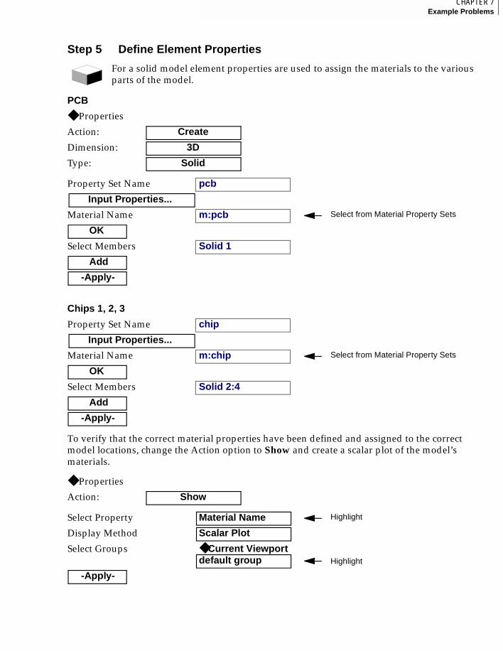
179CHAPTER 7Example Problems
7
Step 5 Define Element Properties
To verify that the correct material properties have been defined and assigned to the correct model locations, change the Action option to Show and create a scalar plot of the model’s materials.
For a solid model element properties are used to assign the materials to the various parts of the model.
PCB
◆ Properties
Action: Create
Dimension: 3D
Type: Solid
Property Set Name pcb
Input Properties...
Material Name m:pcb Select from Material Property Sets
OK
Select Members Solid 1
Add
-Apply-
Chips 1, 2, 3
Property Set Name chip
Input Properties...
Material Name m:chip Select from Material Property Sets
OK
Select Members Solid 2:4
Add
-Apply-
◆ Properties
Action: Show
Select Property Material Name Highlight
Display Method Scalar Plot
Select Groups ◆ Current Viewportdefault group Highlight
-Apply-
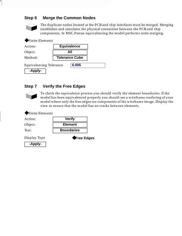
7
180
Step 6 Merge the Common Nodes
The duplicate nodes located at the PCB and chip interfaces must be merged. Merging establishes and simulates the physical connection between the PCB and chip components. In MSC.Patran equivalencing the model performs node merging.
◆ Finite Elements
Action: Equivalence
Object: All
Method: Tolerance Cube
Equivalencing Tolerance 0.005
-Apply-
Step 7 Verify the Free Edges
To check the equivalence process you should verify the element boundaries. If the model has been equivalenced properly you should see a wireframe rendering of your model where only the free edges are components of the wireframe image. Display the view to ensure that the model has no cracks between elements.
◆ Finite Elements
Action: Verify
Object: Element
Test: Boundaries
Display Type ◆ Free Edges
-Apply-
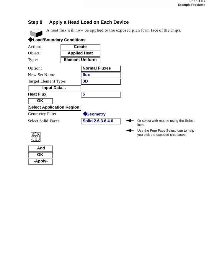
181CHAPTER 7Example Problems
7
Step 8 Apply a Head Load on Each Device
A heat flux will now be applied to the exposed plan form face of the chips.
◆ Load/Boundary Conditions
Action: Create
Object: Applied Heat
Type: Element Uniform
Option: Normal Fluxes
New Set Name flux
Target Element Type: 3D
Input Data...
Heat Flux 5
OK
Select Application Region
Geometry Filter ◆ Geometry
Select Solid Faces Solid 2.6 3.6 4.6 Or select with mouse using the Select icon.
Use the Free Face Select icon to help you pick the exposed chip faces.
Add
OK
-Apply-
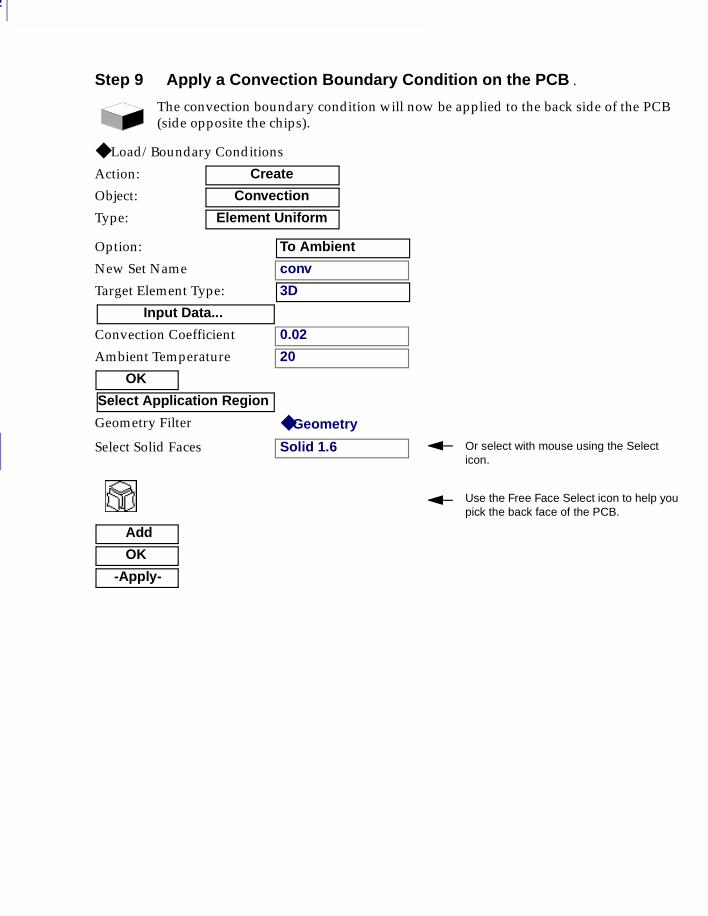
7
182
Step 9 Apply a Convection Boundary Condition on the PCB .
The convection boundary condition will now be applied to the back side of the PCB (side opposite the chips).
◆ Load/Boundary Conditions
Action: Create
Object: Convection
Type: Element Uniform
Option: To Ambient
New Set Name conv
Target Element Type: 3D
Input Data...
Convection Coefficient 0.02
Ambient Temperature 20
OK
Select Application Region
Geometry Filter ◆ Geometry
Select Solid Faces Solid 1.6 Or select with mouse using the Select icon.
Use the Free Face Select icon to help youpick the back face of the PCB.
Add
OK
-Apply-
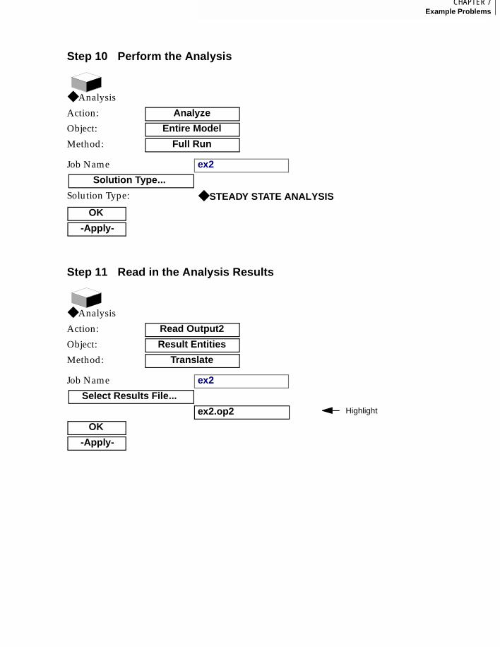
183CHAPTER 7Example Problems
7
Step 10 Perform the Analysis
◆ Analysis
Action: Analyze
Object: Entire Model
Method: Full Run
Job Name ex2
Solution Type...
Solution Type: ◆ STEADY STATE ANALYSIS
OK
-Apply-
Step 11 Read in the Analysis Results
◆ Analysis
Action: Read Output2
Object: Result Entities
Method: Translate
Job Name ex2
Select Results File...
ex2.op2 Highlight
OK
-Apply-
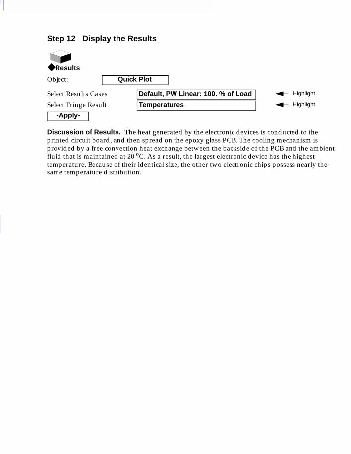
7
184
Step 12 Display the Results
Discussion of Results. The heat generated by the electronic devices is conducted to the printed circuit board, and then spread on the epoxy glass PCB. The cooling mechanism is provided by a free convection heat exchange between the backside of the PCB and the ambient fluid that is maintained at 20 oC. As a result, the largest electronic device has the highest temperature. Because of their identical size, the other two electronic chips possess nearly the same temperature distribution.
◆ Results
Object: Quick Plot
Select Results Cases Default, PW Linear: 100. % of Load Highlight
Select Fringe Result Temperatures Highlight
-Apply-
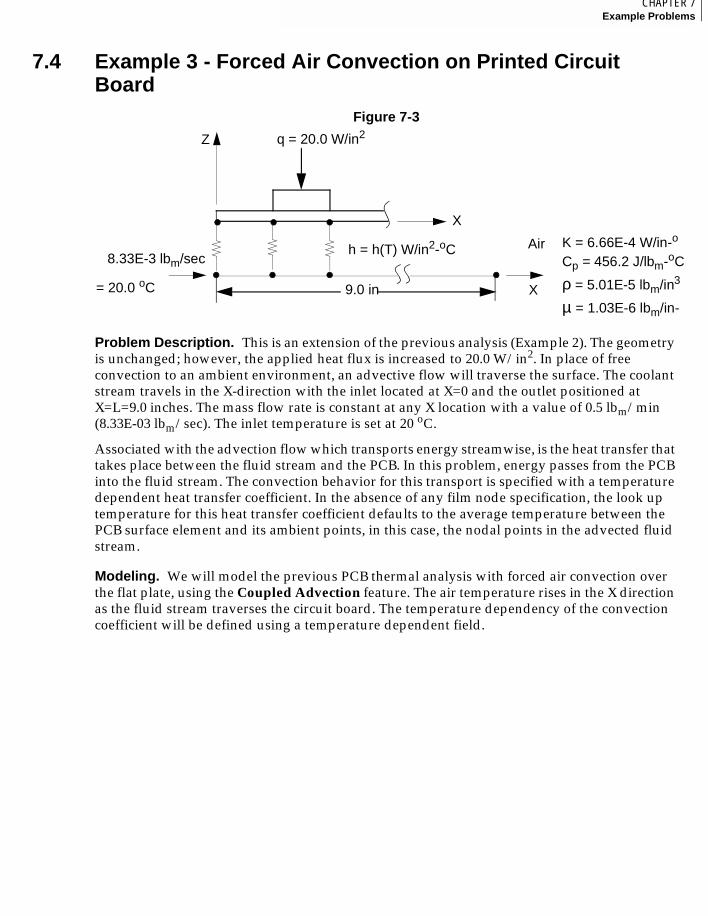
185CHAPTER 7Example Problems
7
7.4 Example 3 - Forced Air Convection on Printed Circuit Board
Figure 7-3
Problem Description. This is an extension of the previous analysis (Example 2). The geometry is unchanged; however, the applied heat flux is increased to 20.0 W/in2. In place of free convection to an ambient environment, an advective flow will traverse the surface. The coolant stream travels in the X-direction with the inlet located at X=0 and the outlet positioned at X=L=9.0 inches. The mass flow rate is constant at any X location with a value of 0.5 lbm/min (8.33E-03 lbm/sec). The inlet temperature is set at 20 oC.
Associated with the advection flow which transports energy streamwise, is the heat transfer that takes place between the fluid stream and the PCB. In this problem, energy passes from the PCB into the fluid stream. The convection behavior for this transport is specified with a temperature dependent heat transfer coefficient. In the absence of any film node specification, the look up temperature for this heat transfer coefficient defaults to the average temperature between the PCB surface element and its ambient points, in this case, the nodal points in the advected fluid stream.
Modeling. We will model the previous PCB thermal analysis with forced air convection over the flat plate, using the Coupled Advection feature. The air temperature rises in the X direction as the fluid stream traverses the circuit board. The temperature dependency of the convection coefficient will be defined using a temperature dependent field.
q = 20.0 W/in2
= 20.0 oC
h = h(T) W/in2-oC
9.0 in
Air K = 6.66E-4 W/in-o
Cp = 456.2 J/lbm-oC
ρ = 5.01E-5 lbm/in3
µ = 1.03E-6 lbm/in-
8.33E-3 lbm/sec
Z
X
X
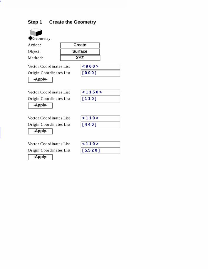
7
186
Step 1 Create the Geometry
◆ Geometry
Action: Create
Object: Surface
Method: XYZ
Vector Coordinates List < 9 6 0 >
Origin Coordinates List [ 0 0 0 ]
-Apply-
Vector Coordinates List < 1 1.5 0 >
Origin Coordinates List [ 1 1 0 ]
-Apply-
Vector Coordinates List < 1 1 0 >
Origin Coordinates List [ 4 4 0 ]
-Apply-
Vector Coordinates List < 1 1 0 >
Origin Coordinates List [ 5.5 2 0 ]
-Apply-
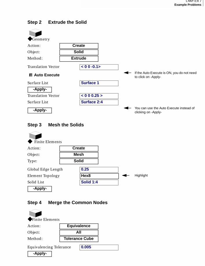
187CHAPTER 7Example Problems
7
Step 2 Extrude the Solid
◆ Geometry
Action: Create
Object: Solid
Method: Extrude
Translation Vector < 0 0 -0.1>
Auto Execute If the Auto Execute is ON, you do not needto click on -Apply-
Surface List Surface 1
-Apply-
Translation Vector < 0 0 0.25 >
Surface List Surface 2:4
-Apply- You can use the Auto Execute instead of clicking on -Apply-
Step 3 Mesh the Solids
◆ Finite Elements
Action: Create
Object: Mesh
Type: Solid
Global Edge Length 0.25
Element Topology Hex8 Highlight
Solid List Solid 1:4
-Apply-
Step 4 Merge the Common Nodes
◆ Finite Elements
Action: Equivalence
Object: All
Method: Tolerance Cube
Equivalencing Tolerance 0.005
-Apply-
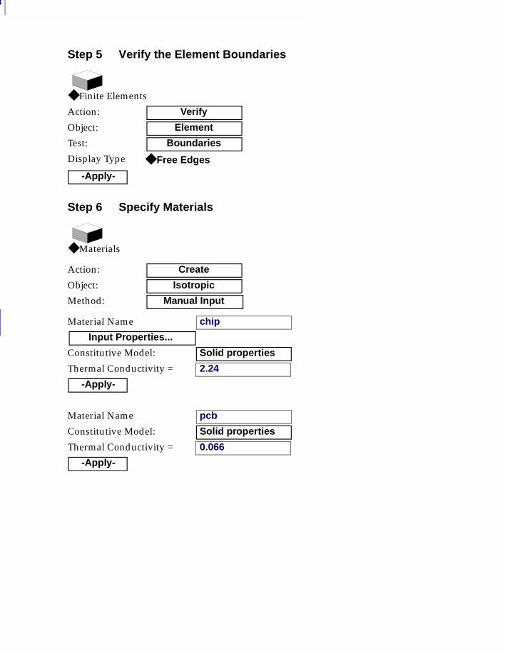
7
188
Step 5 Verify the Element Boundaries
◆ Finite Elements
Action: Verify
Object: Element
Test: Boundaries
Display Type ◆ Free Edges
-Apply-
Step 6 Specify Materials
◆ Materials
Action: Create
Object: Isotropic
Method: Manual Input
Material Name chip
Input Properties...
Constitutive Model: Solid properties
Thermal Conductivity = 2.24
-Apply-
Material Name pcb
Constitutive Model: Solid properties
Thermal Conductivity = 0.066
-Apply-
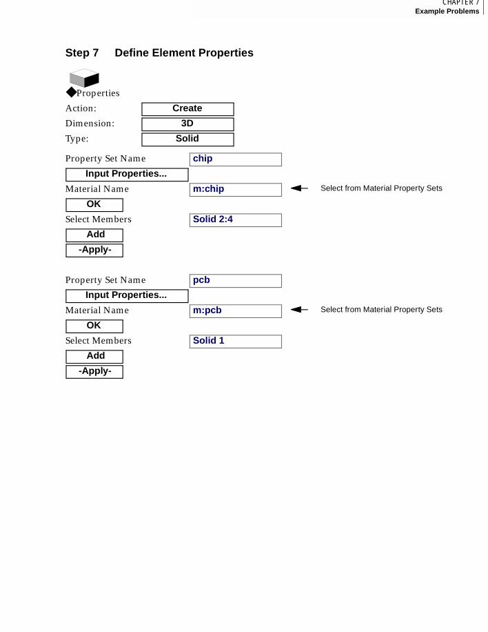
189CHAPTER 7Example Problems
7
Step 7 Define Element Properties
◆ Properties
Action: Create
Dimension: 3D
Type: Solid
Property Set Name chip
Input Properties...
Material Name m:chip Select from Material Property Sets
OK
Select Members Solid 2:4
Add
-Apply-
Property Set Name pcb
Input Properties...
Material Name m:pcb Select from Material Property Sets
OK
Select Members Solid 1
Add
-Apply-
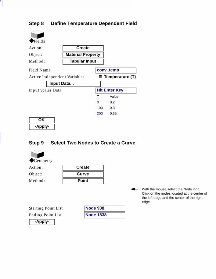
7
190
Step 8 Define Temperature Dependent Field
◆ Fields
Action: Create
Object: Material Property
Method: Tabular Input
Field Name conv_temp
Active Independent Variables Temperature (T)
Input Data...
Input Scalar Data Hit Enter KeyT
0
100
200
Value
0.2
0.3
0.35
OK
-Apply-
Step 9 Select Two Nodes to Create a Curve
◆ Geometry
Action: Create
Object: Curve
Method: Point
With the mouse select the Node icon. Click on the nodes located at the center ofthe left edge and the center of the right edge.
Starting Point List Node 938
Ending Point List Node 1838
-Apply-
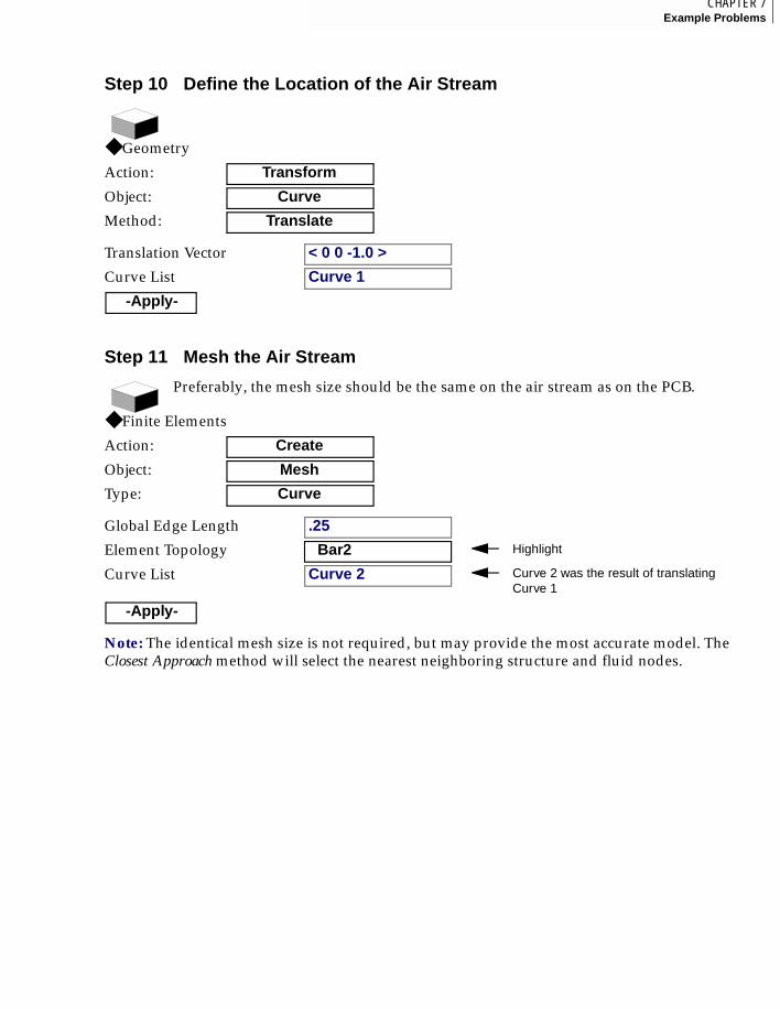
191CHAPTER 7Example Problems
7
Step 10 Define the Location of the Air Stream
◆ Geometry
Action: Transform
Object: Curve
Method: Translate
Translation Vector < 0 0 -1.0 >
Curve List Curve 1
-Apply-
Step 11 Mesh the Air Stream
Note: The identical mesh size is not required, but may provide the most accurate model. The Closest Approach method will select the nearest neighboring structure and fluid nodes.
Preferably, the mesh size should be the same on the air stream as on the PCB.
◆ Finite Elements
Action: Create
Object: Mesh
Type: Curve
Global Edge Length .25
Element Topology Bar2 Highlight
Curve List Curve 2 Curve 2 was the result of translating Curve 1
-Apply-
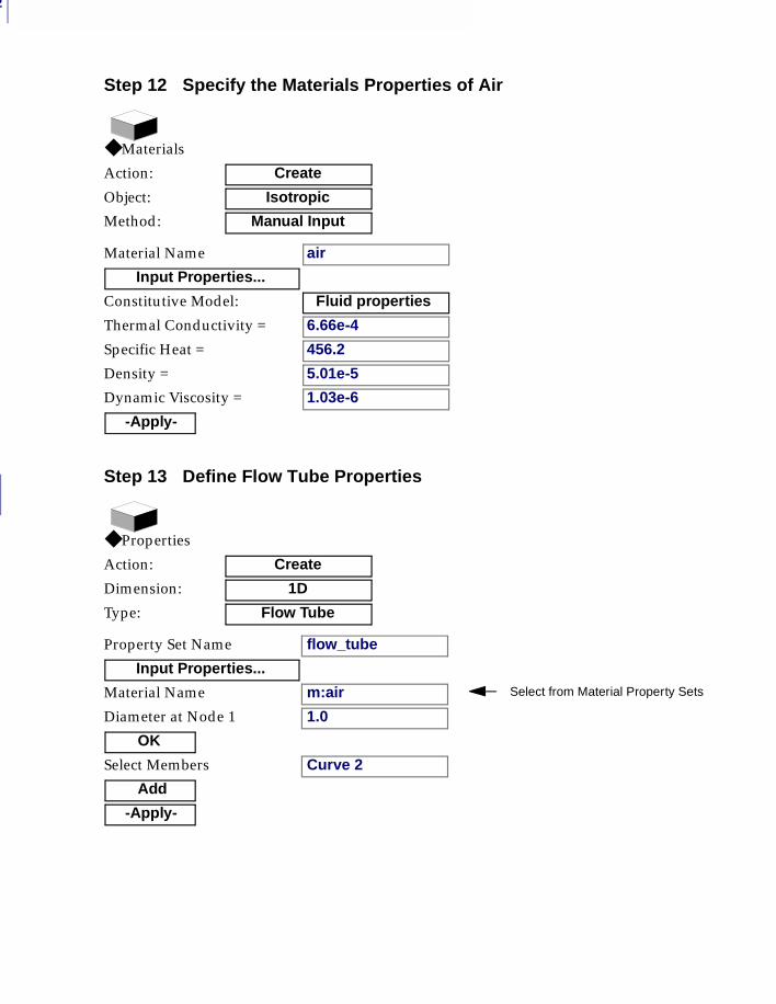
7
192
Step 12 Specify the Materials Properties of Air
◆ Materials
Action: Create
Object: Isotropic
Method: Manual Input
Material Name air
Input Properties...
Constitutive Model: Fluid properties
Thermal Conductivity = 6.66e-4
Specific Heat = 456.2
Density = 5.01e-5
Dynamic Viscosity = 1.03e-6
-Apply-
Step 13 Define Flow Tube Properties
◆ Properties
Action: Create
Dimension: 1D
Type: Flow Tube
Property Set Name flow_tube
Input Properties...
Material Name m:air Select from Material Property Sets
Diameter at Node 1 1.0
OK
Select Members Curve 2
Add
-Apply-
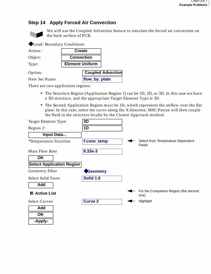
193CHAPTER 7Example Problems
7
Step 14 Apply Forced Air Convection
We will use the Coupled Advection feature to simulate the forced air convection on the back surface of PCB.
◆ Load/Boundary Conditions
Action: Create
Object: Convection
Type: Element Uniform
Option: Coupled Advection
New Set Name flow_by_plate
There are two application regions:
• The Structure Region (Application Region 1) can be 1D, 2D, or 3D. In this case we havea 3D structure, and the appropriate Target Element Type is 3D.
• The Second Application Region must be 1D, which represents the airflow over the flatplate. In this case, select the curve along the X direction. MSC.Patran will then couple the fluid to the structure locally by the Closest Approach method.
Target Element Type: 3D
Region 2: 1D
Input Data...
*Temperature Function f:conv_temp Select from Temperature Dependent Fields
Mass Flow Rate 8.33e-3
OK
Select Application Region
Geometry Filter ◆ Geometry
Select Solid Faces Solid 1.6
Add
Active ListFor the Companion Region (the second one)
Select Curves Curve 2 Highlight
Add
OK
-Apply-
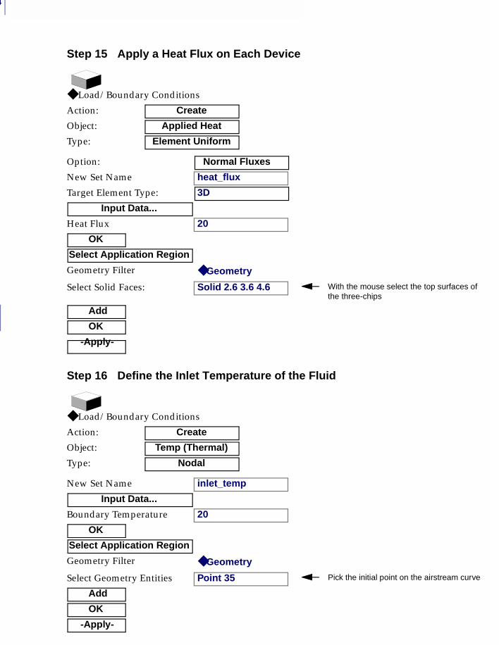
7
194
Step 15 Apply a Heat Flux on Each Device
◆ Load/Boundary Conditions
Action: Create
Object: Applied Heat
Type: Element Uniform
Option: Normal Fluxes
New Set Name heat_flux
Target Element Type: 3D
Input Data...
Heat Flux 20
OK
Select Application Region
Geometry Filter ◆ Geometry
Select Solid Faces: Solid 2.6 3.6 4.6 With the mouse select the top surfaces of the three-chips
Add
OK
-Apply-
Step 16 Define the Inlet Temperature of the Fluid
◆ Load/Boundary Conditions
Action: Create
Object: Temp (Thermal)
Type: Nodal
New Set Name inlet_temp
Input Data...
Boundary Temperature 20
OK
Select Application Region
Geometry Filter ◆ Geometry
Select Geometry Entities Point 35 Pick the initial point on the airstream curve
Add
OK
-Apply-
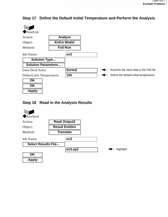
195CHAPTER 7Example Problems
7
Step 17 Define the Default Initial Temperature and Perform the Analysis
◆ Analysis
Action: Analyze
Object: Entire Model
Method: Full Run
Job Name ex3
Solution Type...
Solution Parameters...
Data Deck Echo: Sorted Examine the input data in the F06 file
Default Init Temperature 100 Define the default initial temperature
OK
OK
-Apply-
Step 18 Read in the Analysis Results
◆ Analysis
Action: Read Output2
Object: Result Entities
Method: Translate
Job Name ex3
Select Results File...
ex3.op2 Highlight
OK
-Apply-
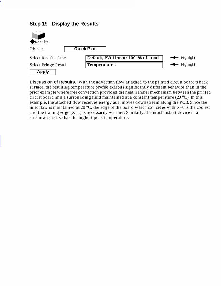
7
196
Step 19 Display the Results
Discussion of Results. With the advection flow attached to the printed circuit board’s back surface, the resulting temperature profile exhibits significantly different behavior than in the prior example where free convection provided the heat transfer mechanism between the printed circuit board and a surrounding fluid maintained at a constant temperature (20 oC). In this example, the attached flow receives energy as it moves downstream along the PCB. Since the inlet flow is maintained at 20 oC, the edge of the board which coincides with X=0 is the coolest and the trailing edge (X=L) is necessarily warmer. Similarly, the most distant device in a streamwise sense has the highest peak temperature.
◆ Results
Object: Quick Plot
Select Results Cases Default, PW Linear: 100. % of Load Highlight
Select Fringe Result Temperatures Highlight
-Apply-
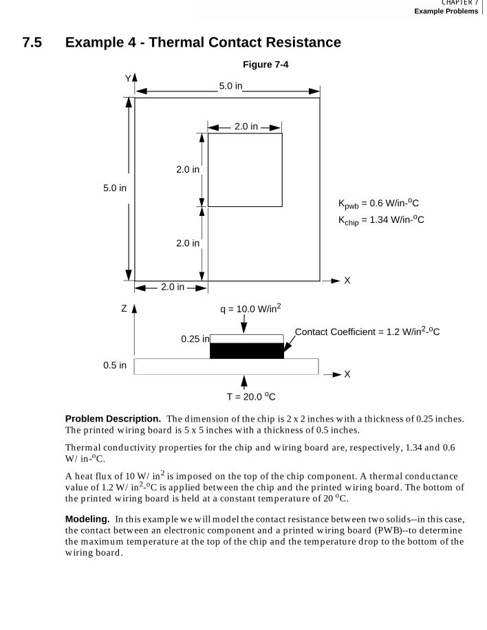
197CHAPTER 7Example Problems
7
7.5 Example 4 - Thermal Contact ResistanceFigure 7-4
Problem Description. The dimension of the chip is 2 x 2 inches with a thickness of 0.25 inches. The printed wiring board is 5 x 5 inches with a thickness of 0.5 inches.
Thermal conductivity properties for the chip and wiring board are, respectively, 1.34 and 0.6 W/in-oC.
A heat flux of 10 W/in2 is imposed on the top of the chip component. A thermal conductance value of 1.2 W/in2-oC is applied between the chip and the printed wiring board. The bottom of the printed wiring board is held at a constant temperature of 20 oC.
Modeling. In this example we will model the contact resistance between two solids--in this case, the contact between an electronic component and a printed wiring board (PWB)--to determine the maximum temperature at the top of the chip and the temperature drop to the bottom of the wiring board.
T = 20.0 oC
5.0 in
5.0 in
Kpwb = 0.6 W/in-oC
Kchip = 1.34 W/in-oC
2.0 in
2.0 in
2.0 in
2.0 in
0.25 in
0.5 in
q = 10.0 W/in2
Contact Coefficient = 1.2 W/in2-oC
Y
X
X
Z
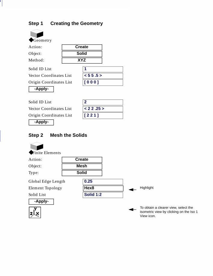
7
198
Step 1 Creating the Geometry
◆ Geometry
Action: Create
Object: Solid
Method: XYZ
Solid ID List 1
Vector Coordinates List < 5 5 .5 >
Origin Coordinates List [ 0 0 0 ]
-Apply-
Solid ID List 2
Vector Coordinates List < 2 2 .25 >
Origin Coordinates List [ 2 2 1 ]
-Apply-
Step 2 Mesh the Solids
◆ Finite Elements
Action: Create
Object: Mesh
Type: Solid
Global Edge Length 0.25
Element Topology Hex8 Highlight
Solid List Solid 1:2
-Apply-To obtain a clearer view, select the isometric view by clicking on the Iso 1 View icon.
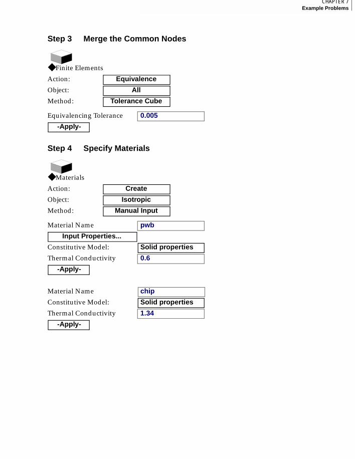
199CHAPTER 7Example Problems
7
Step 3 Merge the Common Nodes
◆ Finite Elements
Action: Equivalence
Object: All
Method: Tolerance Cube
Equivalencing Tolerance 0.005
-Apply-
Step 4 Specify Materials
◆ Materials
Action: Create
Object: Isotropic
Method: Manual Input
Material Name pwb
Input Properties...
Constitutive Model: Solid properties
Thermal Conductivity 0.6
-Apply-
Material Name chip
Constitutive Model: Solid properties
Thermal Conductivity 1.34
-Apply-
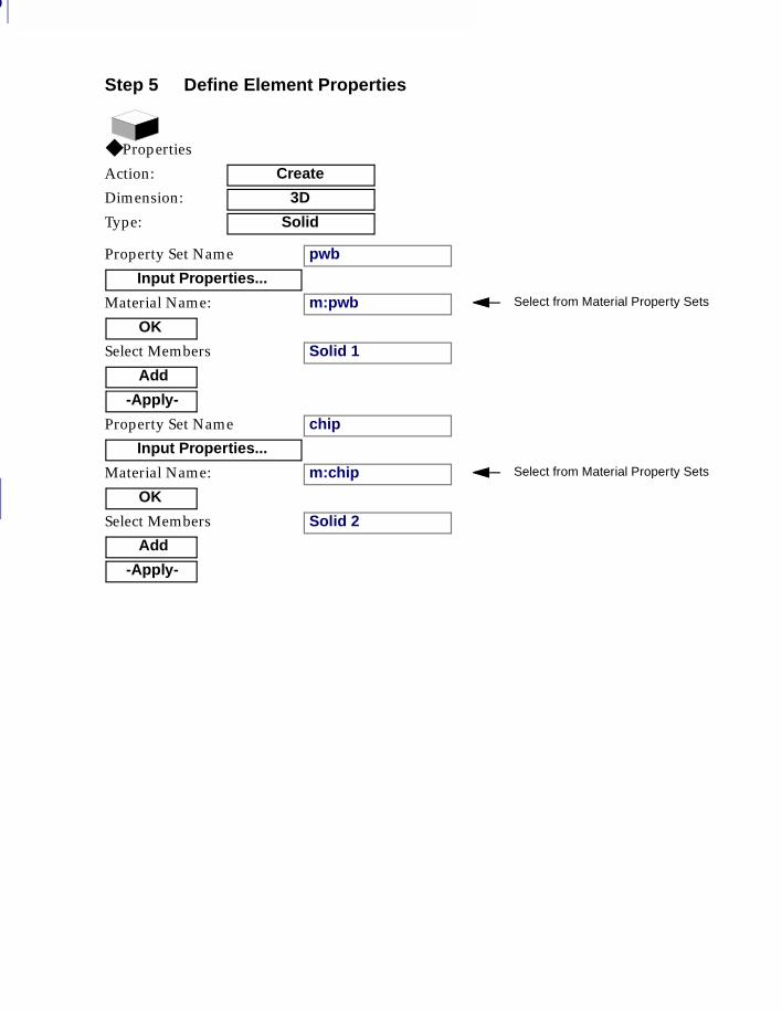
7
200
Step 5 Define Element Properties
◆ Properties
Action: Create
Dimension: 3D
Type: Solid
Property Set Name pwb
Input Properties...
Material Name: m:pwb Select from Material Property Sets
OK
Select Members Solid 1
Add
-Apply-
Property Set Name chip
Input Properties...
Material Name: m:chip Select from Material Property Sets
OK
Select Members Solid 2
Add
-Apply-
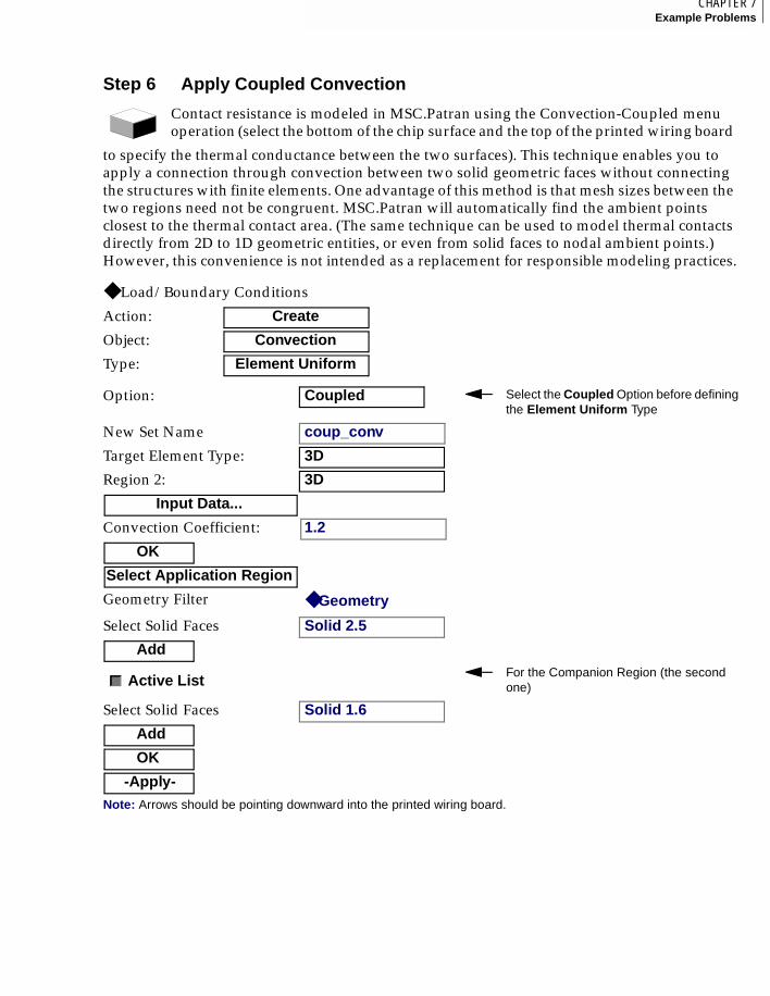
201CHAPTER 7Example Problems
7
Step 6 Apply Coupled Convection
Contact resistance is modeled in MSC.Patran using the Convection-Coupled menu operation (select the bottom of the chip surface and the top of the printed wiring board
to specify the thermal conductance between the two surfaces). This technique enables you to apply a connection through convection between two solid geometric faces without connecting the structures with finite elements. One advantage of this method is that mesh sizes between the two regions need not be congruent. MSC.Patran will automatically find the ambient points closest to the thermal contact area. (The same technique can be used to model thermal contacts directly from 2D to 1D geometric entities, or even from solid faces to nodal ambient points.) However, this convenience is not intended as a replacement for responsible modeling practices.
◆ Load/Boundary Conditions
Action: Create
Object: Convection
Type: Element Uniform
Option: Coupled Select the Coupled Option before definingthe Element Uniform Type
New Set Name coup_conv
Target Element Type: 3D
Region 2: 3D
Input Data...
Convection Coefficient: 1.2
OK
Select Application Region
Geometry Filter ◆ Geometry
Select Solid Faces Solid 2.5
Add
Active ListFor the Companion Region (the second one)
Select Solid Faces Solid 1.6
Add
OK
-Apply-Note: Arrows should be pointing downward into the printed wiring board.
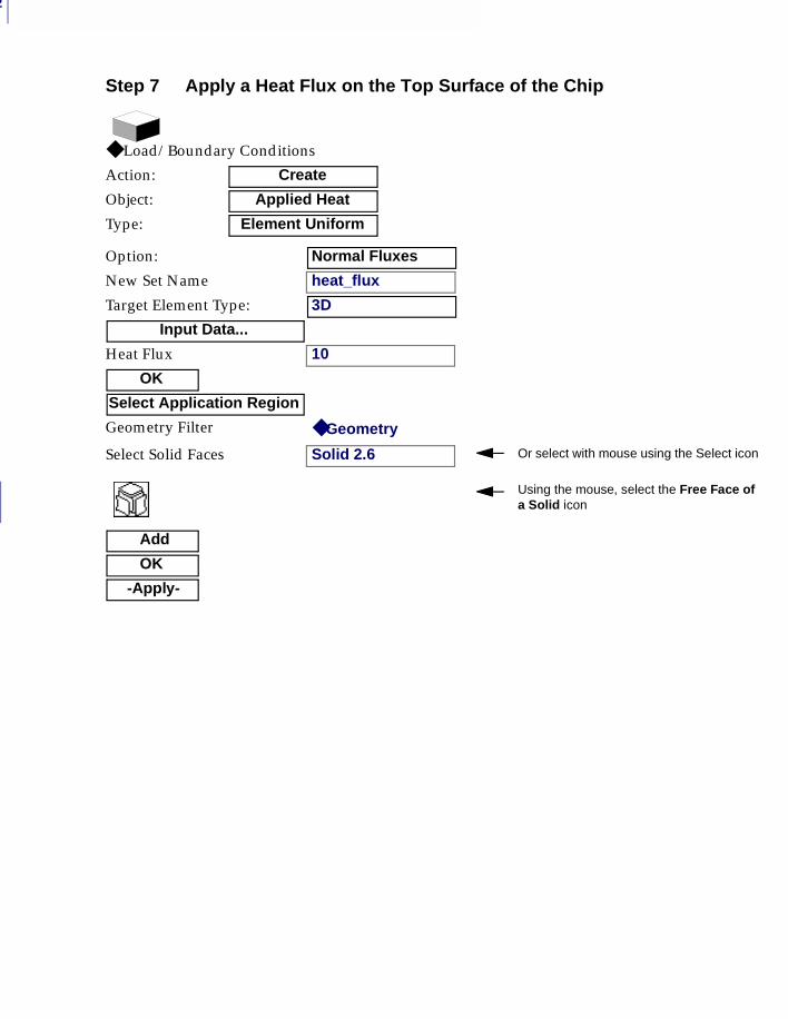
7
202
Step 7 Apply a Heat Flux on the Top Surface of the Chip
◆ Load/Boundary Conditions
Action: Create
Object: Applied Heat
Type: Element Uniform
Option: Normal Fluxes
New Set Name heat_flux
Target Element Type: 3D
Input Data...
Heat Flux 10
OK
Select Application Region
Geometry Filter ◆ Geometry
Select Solid Faces Solid 2.6 Or select with mouse using the Select icon
Using the mouse, select the Free Face ofa Solid icon
Add
OK
-Apply-
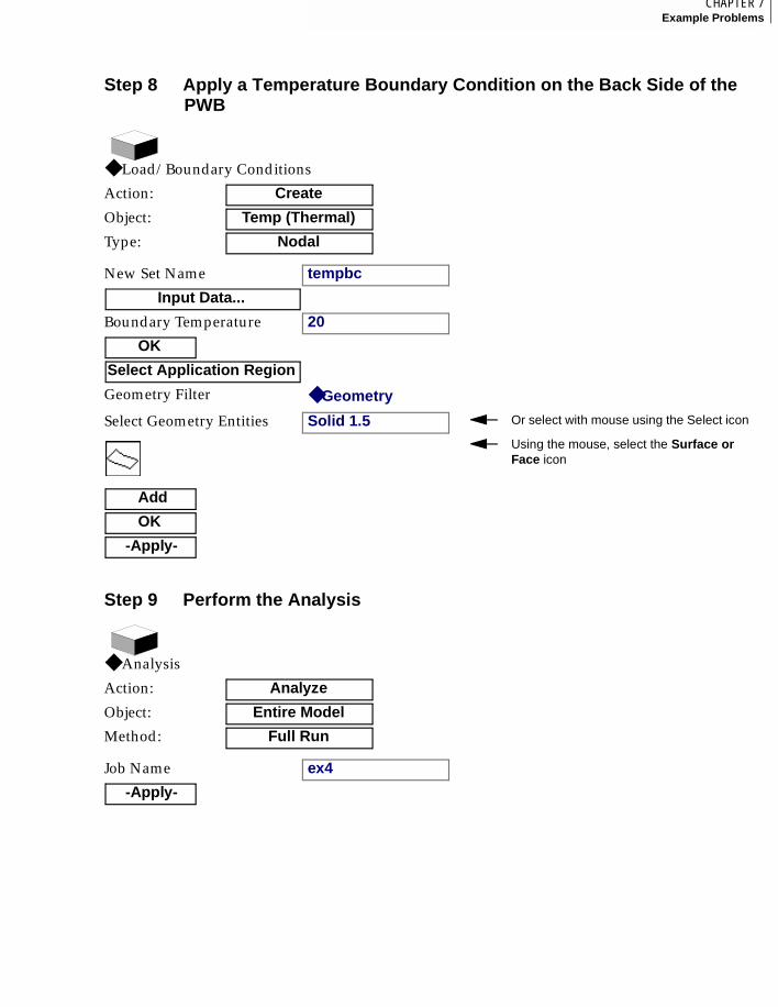
203CHAPTER 7Example Problems
7
Step 8 Apply a Temperature Boundary Condition on the Back Side of the PWB
◆ Load/Boundary Conditions
Action: Create
Object: Temp (Thermal)
Type: Nodal
New Set Name tempbc
Input Data...
Boundary Temperature 20
OK
Select Application Region
Geometry Filter ◆ Geometry
Select Geometry Entities Solid 1.5 Or select with mouse using the Select icon
Using the mouse, select the Surface or Face icon
Add
OK
-Apply-
Step 9 Perform the Analysis
◆ Analysis
Action: Analyze
Object: Entire Model
Method: Full Run
Job Name ex4
-Apply-
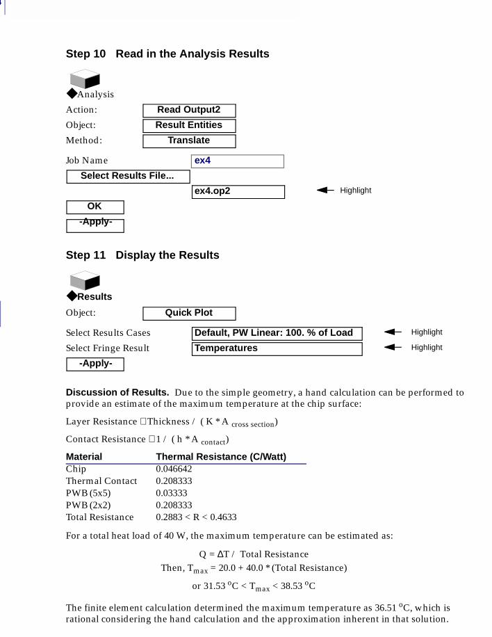
7
204
Discussion of Results. Due to the simple geometry, a hand calculation can be performed to provide an estimate of the maximum temperature at the chip surface:
Layer Resistance ≅ Thickness / ( K * A cross section)
Contact Resistance ≅ 1 / ( h * A contact)
For a total heat load of 40 W, the maximum temperature can be estimated as:
Q = ∆T / Total ResistanceThen, Tmax = 20.0 + 40.0 * (Total Resistance)
or 31.53 oC < Tmax < 38.53 oC
The finite element calculation determined the maximum temperature as 36.51 oC, which is rational considering the hand calculation and the approximation inherent in that solution.
Material Thermal Resistance (C/Watt)Chip 0.046642Thermal Contact 0.208333PWB (5x5) 0.03333PWB (2x2) 0.208333Total Resistance 0.2883 < R < 0.4633
Step 10 Read in the Analysis Results
◆ Analysis
Action: Read Output2
Object: Result Entities
Method: Translate
Job Name ex4
Select Results File...
ex4.op2 Highlight
OK
-Apply-
Step 11 Display the Results
◆ Results
Object: Quick Plot
Select Results Cases Default, PW Linear: 100. % of Load Highlight
Select Fringe Result Temperatures Highlight
-Apply-
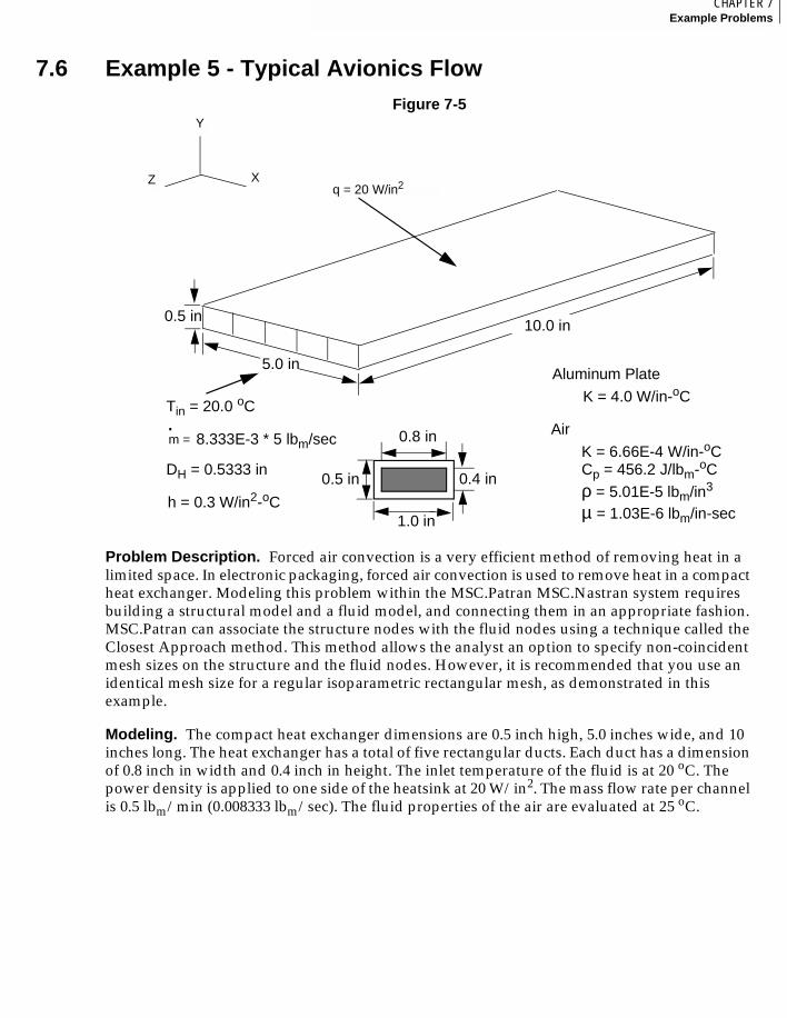
205CHAPTER 7Example Problems
7
7.6 Example 5 - Typical Avionics FlowFigure 7-5
Problem Description. Forced air convection is a very efficient method of removing heat in a limited space. In electronic packaging, forced air convection is used to remove heat in a compact heat exchanger. Modeling this problem within the MSC.Patran MSC.Nastran system requires building a structural model and a fluid model, and connecting them in an appropriate fashion. MSC.Patran can associate the structure nodes with the fluid nodes using a technique called the Closest Approach method. This method allows the analyst an option to specify non-coincident mesh sizes on the structure and the fluid nodes. However, it is recommended that you use an identical mesh size for a regular isoparametric rectangular mesh, as demonstrated in this example.
Modeling. The compact heat exchanger dimensions are 0.5 inch high, 5.0 inches wide, and 10 inches long. The heat exchanger has a total of five rectangular ducts. Each duct has a dimension of 0.8 inch in width and 0.4 inch in height. The inlet temperature of the fluid is at 20 oC. The power density is applied to one side of the heatsink at 20 W/in2. The mass flow rate per channel is 0.5 lbm/min (0.008333 lbm/sec). The fluid properties of the air are evaluated at 25 oC.
10.0 in
5.0 in
Y
XZq = 20 W/in2
0.5 in
m = .
8.333E-3 * 5 lbm/secK = 6.66E-4 W/in-oCCp = 456.2 J/lbm-oC
ρ = 5.01E-5 lbm/in3
µ = 1.03E-6 lbm/in-sec
0.5 in 0.4 in
1.0 in
0.8 in
Tin = 20.0 oC
Air
K = 4.0 W/in-oC
Aluminum Plate
DH = 0.5333 in
h = 0.3 W/in2-oC
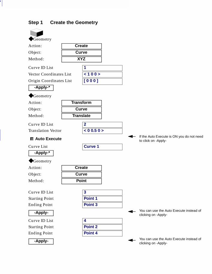
7
206
Step 1 Create the Geometry
◆ Geometry
Action: Create
Object: Curve
Method: XYZ
Curve ID List 1
Vector Coordinates List < 1 0 0 >
Origin Coordinates List [ 0 0 0 ]
-Apply-*
◆ Geometry
Action: Transform
Object: Curve
Method: Translate
Curve ID List 2
Translation Vector < 0 0.5 0 >
Auto ExecuteIf the Auto Execute is ON you do not needto click on -Apply-
Curve List Curve 1
-Apply-*
◆ Geometry
Action: Create
Object: Curve
Method: Point
Curve ID List 3
Starting Point Point 1
Ending Point Point 3
-Apply- You can use the Auto Execute instead of clicking on -Apply-
Curve ID List 4
Starting Point Point 2
Ending Point Point 4
-Apply- You can use the Auto Execute instead of clicking on -Apply-
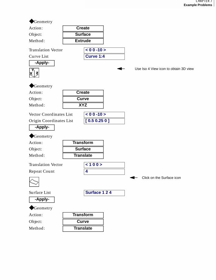
207CHAPTER 7Example Problems
7
◆ GeometryAction: Create
Object: Surface
Method: Extrude
Translation Vector < 0 0 -10 >
Curve List Curve 1:4
-Apply-Use Iso 4 View icon to obtain 3D view
◆ GeometryAction: Create
Object: Curve
Method: XYZ
Vector Coordinates List < 0 0 -10 >
Origin Coordinates List [ 0.5 0.25 0 ]
-Apply-
◆ GeometryAction: Transform
Object: Surface
Method: Translate
Translation Vector < 1 0 0 >
Repeat Count 4Click on the Surface icon
Surface List Surface 1 2 4
-Apply-
◆ Geometry
Action: Transform
Object: Curve
Method: Translate
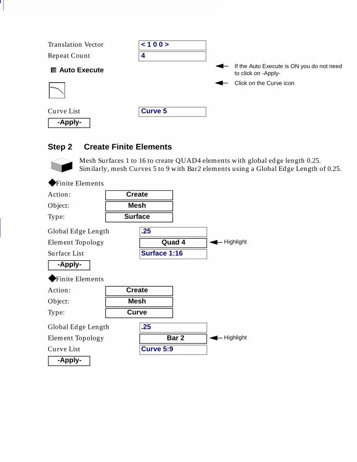
7
208
Translation Vector < 1 0 0 >
Repeat Count 4
Auto ExecuteIf the Auto Execute is ON you do not needto click on -Apply-
Click on the Curve icon
Curve List Curve 5
-Apply-
Step 2 Create Finite Elements
Mesh Surfaces 1 to 16 to create QUAD4 elements with global edge length 0.25. Similarly, mesh Curves 5 to 9 with Bar2 elements using a Global Edge Length of 0.25.
◆ Finite Elements
Action: Create
Object: Mesh
Type: Surface
Global Edge Length .25
Element Topology Quad 4 Highlight
Surface List Surface 1:16
-Apply-
◆ Finite Elements
Action: Create
Object: Mesh
Type: Curve
Global Edge Length .25
Element Topology Bar 2 Highlight
Curve List Curve 5:9
-Apply-
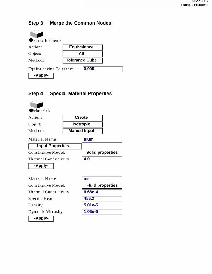
209CHAPTER 7Example Problems
7
Step 3 Merge the Common Nodes
◆ Finite Elements
Action: Equivalence
Object: All
Method: Tolerance Cube
Equivalencing Tolerance 0.005
-Apply-
Step 4 Special Material Properties
◆ Materials
Action: Create
Object: Isotropic
Method: Manual Input
Material Name alum
Input Properties...
Constitutive Model: Solid properties
Thermal Conductivity 4.0
-Apply-
Material Name air
Constitutive Model: Fluid properties
Thermal Conductivity 6.66e-4
Specific Heat 456.2
Density 5.01e-5
Dynamic Viscosity 1.03e-6
-Apply-
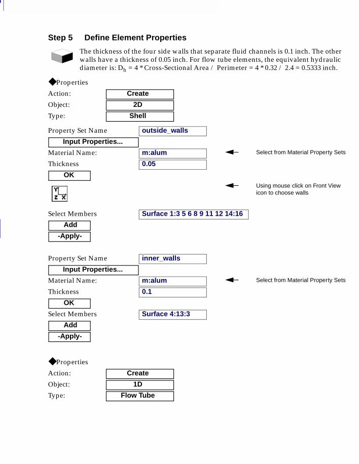
7
210
Step 5 Define Element Properties
The thickness of the four side walls that separate fluid channels is 0.1 inch. The other walls have a thickness of 0.05 inch. For flow tube elements, the equivalent hydraulic diameter is: Dh = 4 * Cross-Sectional Area / Perimeter = 4 * 0.32 / 2.4 = 0.5333 inch.
◆ Properties
Action: Create
Object: 2D
Type: Shell
Property Set Name outside_walls
Input Properties...
Material Name: m:alum Select from Material Property Sets
Thickness 0.05
OKUsing mouse click on Front View icon to choose walls
Select Members Surface 1:3 5 6 8 9 11 12 14:16
Add
-Apply-
Property Set Name inner_walls
Input Properties...
Material Name: m:alum Select from Material Property Sets
Thickness 0.1
OK
Select Members Surface 4:13:3
Add
-Apply-
◆ Properties
Action: Create
Object: 1D
Type: Flow Tube
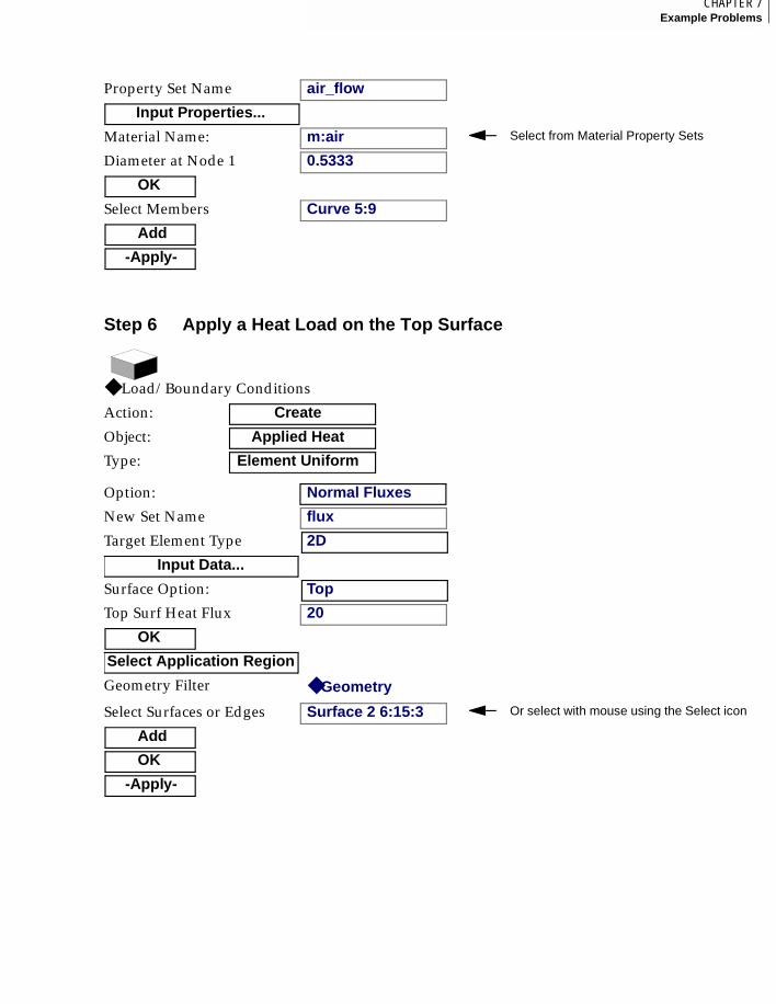
211CHAPTER 7Example Problems
7
Property Set Name air_flow
Input Properties...
Material Name: m:air Select from Material Property Sets
Diameter at Node 1 0.5333
OK
Select Members Curve 5:9
Add
-Apply-
Step 6 Apply a Heat Load on the Top Surface
◆ Load/Boundary Conditions
Action: Create
Object: Applied Heat
Type: Element Uniform
Option: Normal Fluxes
New Set Name flux
Target Element Type 2D
Input Data...
Surface Option: Top
Top Surf Heat Flux 20
OK
Select Application Region
Geometry Filter ◆ Geometry
Select Surfaces or Edges Surface 2 6:15:3 Or select with mouse using the Select icon
Add
OK
-Apply-
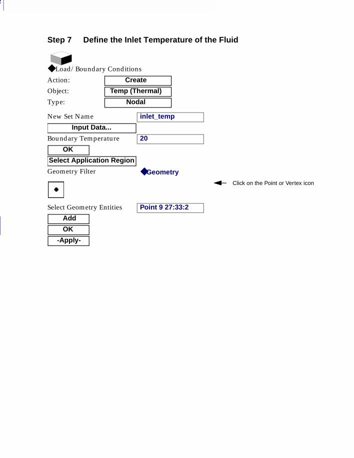
7
212
Step 7 Define the Inlet Temperature of the Fluid
◆ Load/Boundary Conditions
Action: Create
Object: Temp (Thermal)
Type: Nodal
New Set Name inlet_temp
Input Data...
Boundary Temperature 20
OK
Select Application Region
Geometry Filter ◆ Geometry
Click on the Point or Vertex icon
Select Geometry Entities Point 9 27:33:2
Add
OK
-Apply-
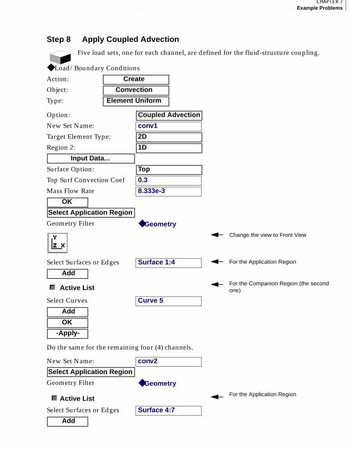
213CHAPTER 7Example Problems
7
Step 8 Apply Coupled Advection
Do the same for the remaining four (4) channels.
Five load sets, one for each channel, are defined for the fluid-structure coupling.
◆ Load/Boundary Conditions
Action: Create
Object: Convection
Type: Element Uniform
Option: Coupled Advection
New Set Name: conv1
Target Element Type: 2D
Region 2: 1D
Input Data...
Surface Option: Top
Top Surf Convection Coef 0.3
Mass Flow Rate 8.333e-3
OK
Select Application Region
Geometry Filter ◆ Geometry
Change the view to Front View
Select Surfaces or Edges Surface 1:4 For the Application Region
Add
Active ListFor the Companion Region (the second one)
Select Curves Curve 5
Add
OK
-Apply-
New Set Name: conv2
Select Application Region
Geometry Filter ◆ Geometry
Active ListFor the Application Region
Select Surfaces or Edges Surface 4:7
Add
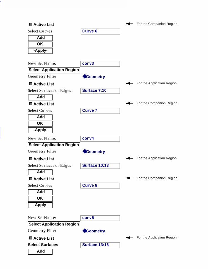
7
214
Active List For the Companion Region
Select Curves Curve 6
Add
OK
-Apply-
New Set Name: conv3
Select Application Region
Geometry Filter ◆ Geometry
Active List For the Application Region
Select Surfaces or Edges Surface 7:10
Add
Active List For the Companion Region
Select Curves Curve 7
Add
OK
-Apply-
New Set Name: conv4
Select Application Region
Geometry Filter ◆ Geometry
Active List For the Application Region
Select Surfaces or Edges Surface 10:13
Add
Active List For the Companion Region
Select Curves Curve 8
Add
OK
-Apply-
New Set Name: conv5
Select Application Region
Geometry Filter ◆ Geometry
Active List For the Application Region
Select Surfaces Surface 13:16
Add
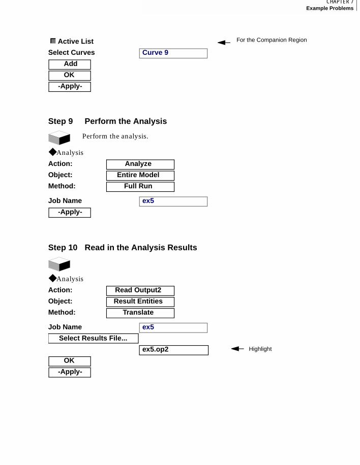
215CHAPTER 7Example Problems
7
Active List For the Companion Region
Select Curves Curve 9
Add
OK
-Apply-
Step 9 Perform the Analysis
Perform the analysis.
◆ Analysis
Action: Analyze
Object: Entire Model
Method: Full Run
Job Name ex5
-Apply-
Step 10 Read in the Analysis Results
◆ Analysis
Action: Read Output2
Object: Result Entities
Method: Translate
Job Name ex5
Select Results File...
ex5.op2 Highlight
OK
-Apply-
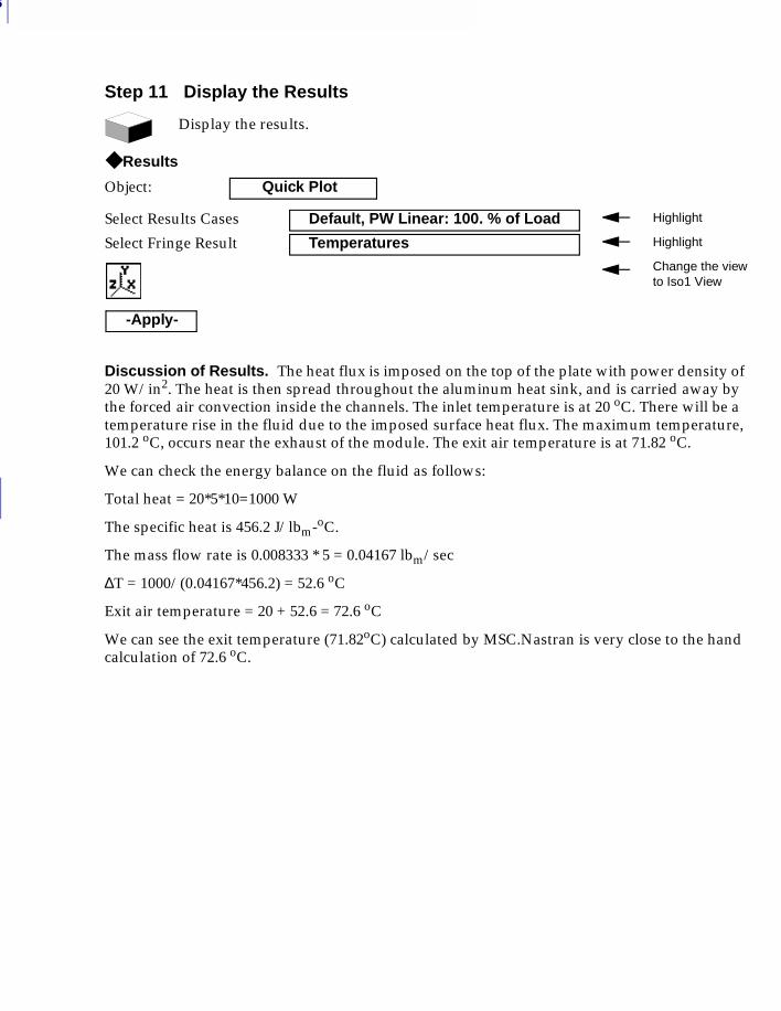
7
216
Discussion of Results. The heat flux is imposed on the top of the plate with power density of 20 W/in2. The heat is then spread throughout the aluminum heat sink, and is carried away by the forced air convection inside the channels. The inlet temperature is at 20 oC. There will be a temperature rise in the fluid due to the imposed surface heat flux. The maximum temperature, 101.2 oC, occurs near the exhaust of the module. The exit air temperature is at 71.82 oC.
We can check the energy balance on the fluid as follows:
Total heat = 20*5*10=1000 W
The specific heat is 456.2 J/lbm-oC.
The mass flow rate is 0.008333 * 5 = 0.04167 lbm/sec
∆T = 1000/(0.04167*456.2) = 52.6 oC
Exit air temperature = 20 + 52.6 = 72.6 oC
We can see the exit temperature (71.82oC) calculated by MSC.Nastran is very close to the hand calculation of 72.6 oC.
Step 11 Display the Results
Display the results.
◆ Results
Object: Quick Plot
Select Results Cases Default, PW Linear: 100. % of Load Highlight
Select Fringe Result Temperatures Highlight
Change the view to Iso1 View
-Apply-
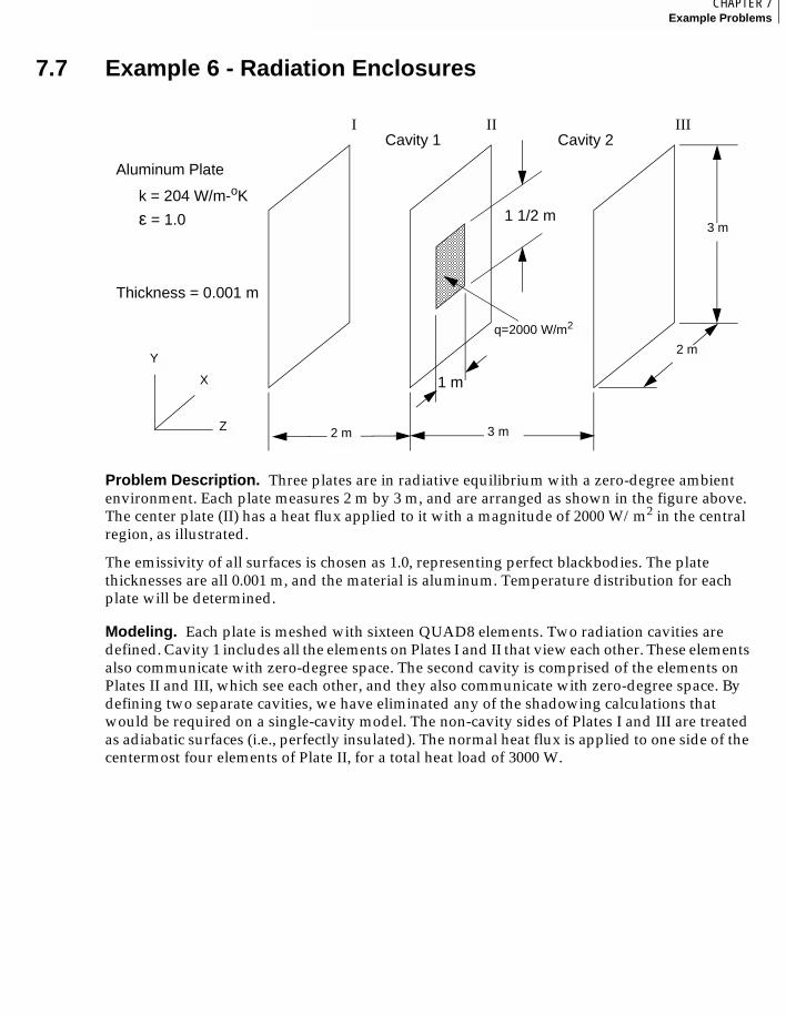
217CHAPTER 7Example Problems
7
7.7 Example 6 - Radiation Enclosures
Problem Description. Three plates are in radiative equilibrium with a zero-degree ambient environment. Each plate measures 2 m by 3 m, and are arranged as shown in the figure above. The center plate (II) has a heat flux applied to it with a magnitude of 2000 W/m2 in the central region, as illustrated.
The emissivity of all surfaces is chosen as 1.0, representing perfect blackbodies. The plate thicknesses are all 0.001 m, and the material is aluminum. Temperature distribution for each plate will be determined.
Modeling. Each plate is meshed with sixteen QUAD8 elements. Two radiation cavities are defined. Cavity 1 includes all the elements on Plates I and II that view each other. These elements also communicate with zero-degree space. The second cavity is comprised of the elements on Plates II and III, which see each other, and they also communicate with zero-degree space. By defining two separate cavities, we have eliminated any of the shadowing calculations that would be required on a single-cavity model. The non-cavity sides of Plates I and III are treated as adiabatic surfaces (i.e., perfectly insulated). The normal heat flux is applied to one side of the centermost four elements of Plate II, for a total heat load of 3000 W.
I II III
1 m
1 1/2 m
2 m
2 m 3 m
3 m
q=2000 W/m2
Z
Y
X
k = 204 W/m-oK
Aluminum Plate
Thickness = 0.001 m
ε = 1.0
Cavity 1 Cavity 2
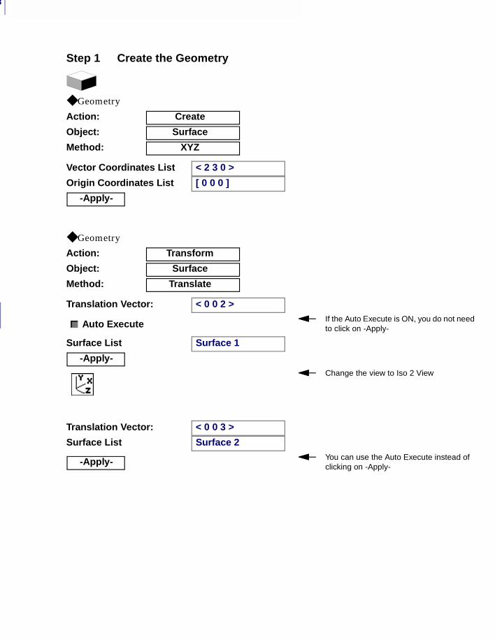
7
218
Step 1 Create the Geometry
◆ Geometry
Action: Create
Object: Surface
Method: XYZ
Vector Coordinates List < 2 3 0 >
Origin Coordinates List [ 0 0 0 ]
-Apply-
◆ Geometry
Action: Transform
Object: Surface
Method: Translate
Translation Vector: < 0 0 2 >
Auto ExecuteIf the Auto Execute is ON, you do not needto click on -Apply-
Surface List Surface 1
-Apply-Change the view to Iso 2 View
Translation Vector: < 0 0 3 >
Surface List Surface 2
-Apply- You can use the Auto Execute instead of clicking on -Apply-
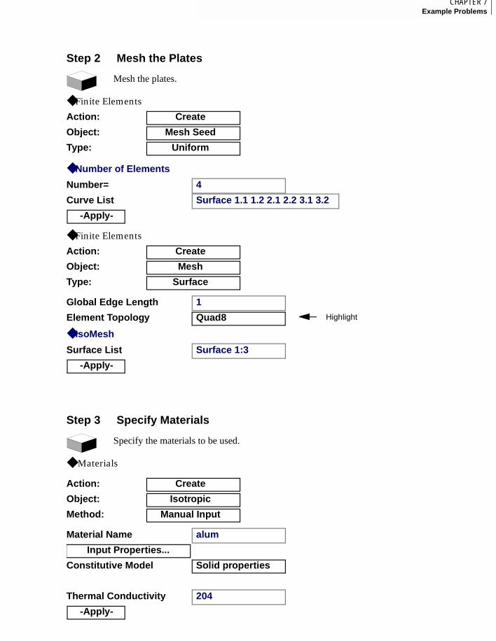
219CHAPTER 7Example Problems
7
Step 2 Mesh the Plates
Mesh the plates.
◆ Finite Elements
Action: Create
Object: Mesh Seed
Type: Uniform
◆ Number of Elements
Number= 4
Curve List Surface 1.1 1.2 2.1 2.2 3.1 3.2
-Apply-
◆ Finite Elements
Action: Create
Object: Mesh
Type: Surface
Global Edge Length 1
Element Topology Quad8 Highlight
◆ IsoMesh
Surface List Surface 1:3
-Apply-
Step 3 Specify Materials
Specify the materials to be used.
◆ Materials
Action: Create
Object: Isotropic
Method: Manual Input
Material Name alum
Input Properties...
Constitutive Model Solid properties
Thermal Conductivity 204
-Apply-
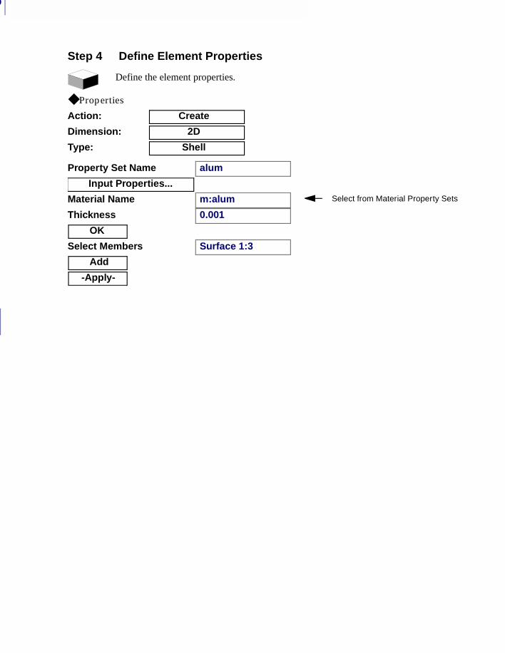
7
220
Step 4 Define Element Properties
Define the element properties.
◆ Properties
Action: Create
Dimension: 2D
Type: Shell
Property Set Name alum
Input Properties...
Material Name m:alum Select from Material Property Sets
Thickness 0.001
OK
Select Members Surface 1:3
Add
-Apply-
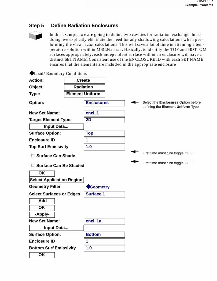
221CHAPTER 7Example Problems
7
Step 5 Define Radiation Enclosures
In this example, we are going to define two cavities for radiation exchange. In so doing, we explicitly eliminate the need for any shadowing calculations when per-forming the view factor calculations. This will save a lot of time in attaining a tem-perature solution within MSC.Nastran. Basically, to identify the TOP and BOTTOM surfaces appropriately, each independent surface within an enclosure will have a distinct SET NAME. Consistent use of the ENCLOSURE ID with each SET NAME ensures that the elements are included in the appropriate enclosure
◆ Load/Boundary Conditions
Action: Create
Object: Radiation
Type: Element Uniform
Option: Enclosures Select the Enclosures Option before defining the Element Uniform Type
New Set Name: encl_1
Target Element Type: 2D
Input Data...
Surface Option: Top
Enclosure ID 1
Top Surf Emissivity 1.0
Surface Can ShadeFirst time must turn toggle OFF
Surface Can Be ShadedFirst time must turn toggle OFF
OK
Select Application Region
Geometry Filter ◆ Geometry
Select Surfaces or Edges Surface 1
Add
OK
-Apply-
New Set Name: encl_1a
Input Data...
Surface Option: Bottom
Enclosure ID 1
Bottom Surf Emissivity 1.0
OK
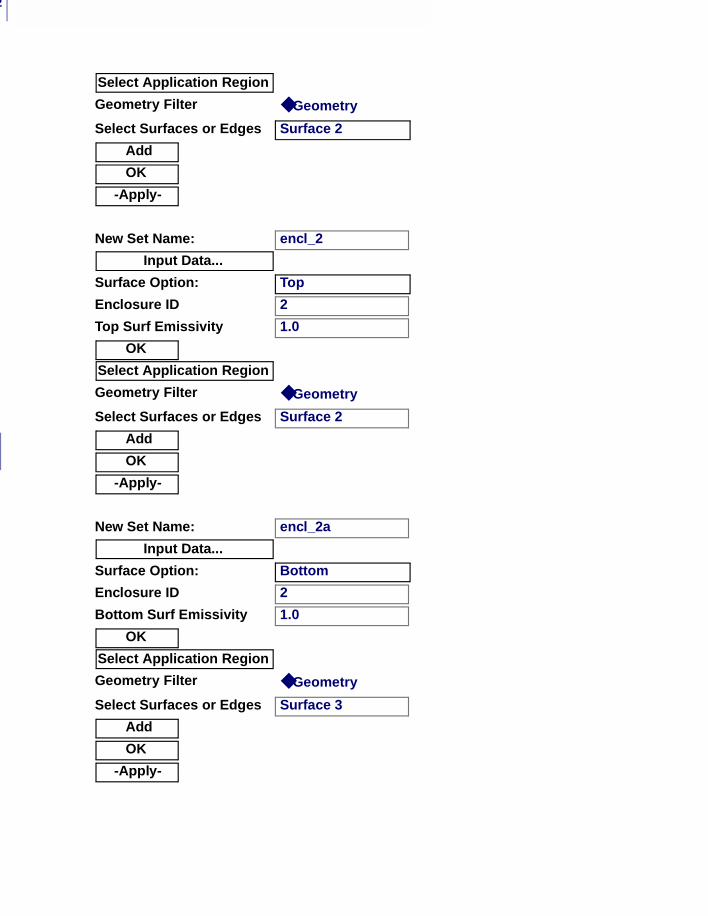
7
222
Select Application Region
Geometry Filter ◆ Geometry
Select Surfaces or Edges Surface 2
Add
OK
-Apply-
New Set Name: encl_2
Input Data...
Surface Option: Top
Enclosure ID 2
Top Surf Emissivity 1.0
OK
Select Application Region
Geometry Filter ◆ Geometry
Select Surfaces or Edges Surface 2
Add
OK
-Apply-
New Set Name: encl_2a
Input Data...
Surface Option: Bottom
Enclosure ID 2
Bottom Surf Emissivity 1.0
OK
Select Application Region
Geometry Filter ◆ Geometry
Select Surfaces or Edges Surface 3
Add
OK
-Apply-
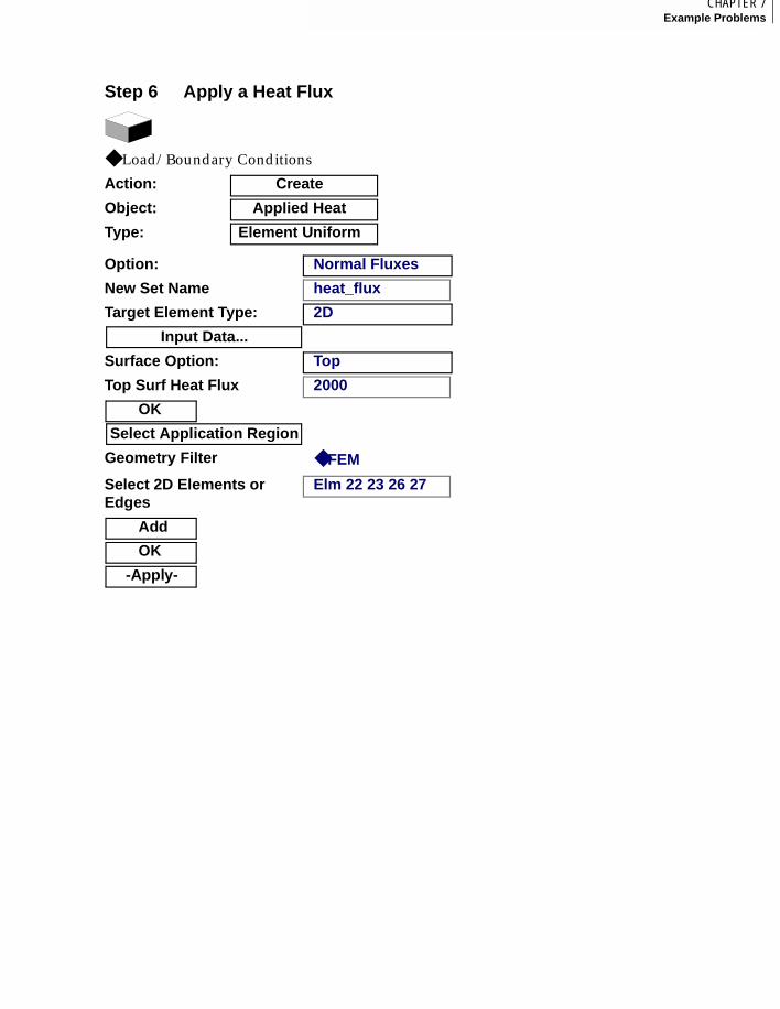
223CHAPTER 7Example Problems
7
Step 6 Apply a Heat Flux
◆ Load/Boundary Conditions
Action: Create
Object: Applied Heat
Type: Element Uniform
Option: Normal Fluxes
New Set Name heat_flux
Target Element Type: 2D
Input Data...
Surface Option: Top
Top Surf Heat Flux 2000
OK
Select Application Region
Geometry Filter ◆ FEM
Select 2D Elements or Edges
Elm 22 23 26 27
Add
OK
-Apply-
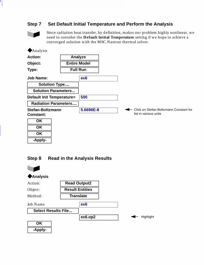
7
224
Step 7 Set Default Initial Temperature and Perform the Analysis
Since radiation heat transfer, by definition, makes our problem highly nonlinear, we need to consider the Default Initial Temperature setting if we hope to achieve a converged solution with the MSC.Nastran thermal solver.
◆ Analysis
Action: Analyze
Object: Entire Model
Type: Full Run
Job Name: ex6
Solution Type....
Solution Parameters...
Default Init Temperature= 500
Radiation Parameters....
Stefan-Boltzmann Constant:
5.6696E-8 Click on Stefan-Boltzmann Constant for list in various units
OK
OK
OK
-Apply-
Step 8 Read in the Analysis Results
◆ Analysis
Action: Read Output2
Object: Result Entities
Method: Translate
Job Name ex6
Select Results File...
ex6.op2 Highlight
OK
-Apply-
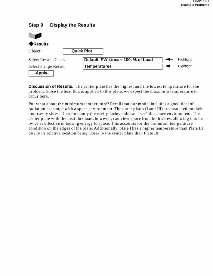
225CHAPTER 7Example Problems
7
Discussion of Results. The center plate has the highest and the lowest temperature for the problem. Since the heat flux is applied to this plate, we expect the maximum temperature to occur here.
But what about the minimum temperature? Recall that our model includes a good deal of radiation exchange with a space environment. The outer plates (I and III) are insulated on their non-cavity sides. Therefore, only the cavity-facing side can “see” the space environment. The center plate with the heat flux load, however, can view space from both sides, allowing it to be twice as effective in loosing energy to space. This accounts for the minimum temperature condition on the edges of the plate. Additionally, plate I has a higher temperature than Plate III due to its relative location being closer to the center plate than Plate III.
Step 9 Display the Results
◆ Results
Object: Quick Plot
Select Results Cases Default, PW Linear: 100. % of Load Highlight
Select Fringe Result Temperatures Highlight
-Apply-
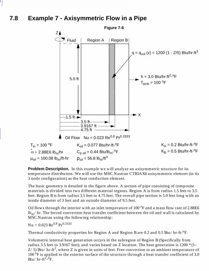
7
226
7.8 Example 7 - Axisymmetric Flow in a PipeFigure 7-6
Problem Description. In this example we will analyze an axisymmetric structure for its temperature distribution. We will use the MSC.Nastran CTRIAX6 axisymmetric element (in its 3 node configuration) as the heat conduction element.
The basic geometry is detailed in the figure above. A section of pipe consisting of composite materials is divided into two different material regions. Region A is from radius 1.5 feet to 3.5 feet. Region B is from radius 3.5 feet to 4.75 feet. The overall pipe section is 5.0 feet long with an inside diameter of 3 feet and an outside diameter of 9.5 feet.
Oil flows through the interior with an inlet temperature of 100 oF and a mass flow rate of 2.88E6 lbm/hr. The forced convection heat transfer coefficient between the oil and wall is calculated by MSC.Nastran using the following relationship:
Nu = 0.023 Re0.8 Pr0.3333
Thermal conductivity properties for Region A and Region B are 0.2 and 0.5 Btu/hr-ft-oF.
Volumetric internal heat generation occurs in the subregion of Region B (Specifically from radius 3.5 feet to 3.9167 feet), and varies based on Z location. The heat generation is 1200 * (1-Z/5) Btu/hr-ft3, where Z is given in units of feet. Free convection to an ambient temperature of 100 oF is applied to the exterior surface of the structure through a heat transfer coefficient of 3.0 Btu/hr-ft2-oF.
5.0 ft
KA = 0.2 Btu/hr-ft-oF
KB = 0.5 Btu/hr-ft-oF
Region A
1.5 ft
q = qvol (z) = 1200 (1 - Z/5) Btu/hr-ft3
3.5 ft3.9167 ft4.75 ft
Region BFluid
Tamb = 100 oF
h = 3.0 Btu/hr-ft2-oF
Oil Flow
X
Z
m = .
2.88E6 lbm/hr
Tin = 100 oF
µoil = 100.08 lbm/ft-hr
Cp oil = 0.44 Btu/lbm-oF
Koil = 0.077 Btu/hr-ft-oF
ρoil = 56.8 lbm/ft3
Nu = 0.023 Re0.8 Pr0.3333
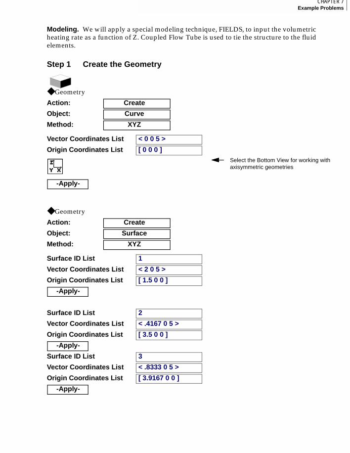
227CHAPTER 7Example Problems
7
Modeling. We will apply a special modeling technique, FIELDS, to input the volumetric heating rate as a function of Z. Coupled Flow Tube is used to tie the structure to the fluid elements.
Step 1 Create the Geometry
◆ Geometry
Action: Create
Object: Curve
Method: XYZ
Vector Coordinates List < 0 0 5 >
Origin Coordinates List [ 0 0 0 ]Select the Bottom View for working with axisymmetric geometries
-Apply-
◆ Geometry
Action: Create
Object: Surface
Method: XYZ
Surface ID List 1
Vector Coordinates List < 2 0 5 >
Origin Coordinates List [ 1.5 0 0 ]
-Apply-
Surface ID List 2
Vector Coordinates List < .4167 0 5 >
Origin Coordinates List [ 3.5 0 0 ]
-Apply-
Surface ID List 3
Vector Coordinates List < .8333 0 5 >
Origin Coordinates List [ 3.9167 0 0 ]
-Apply-
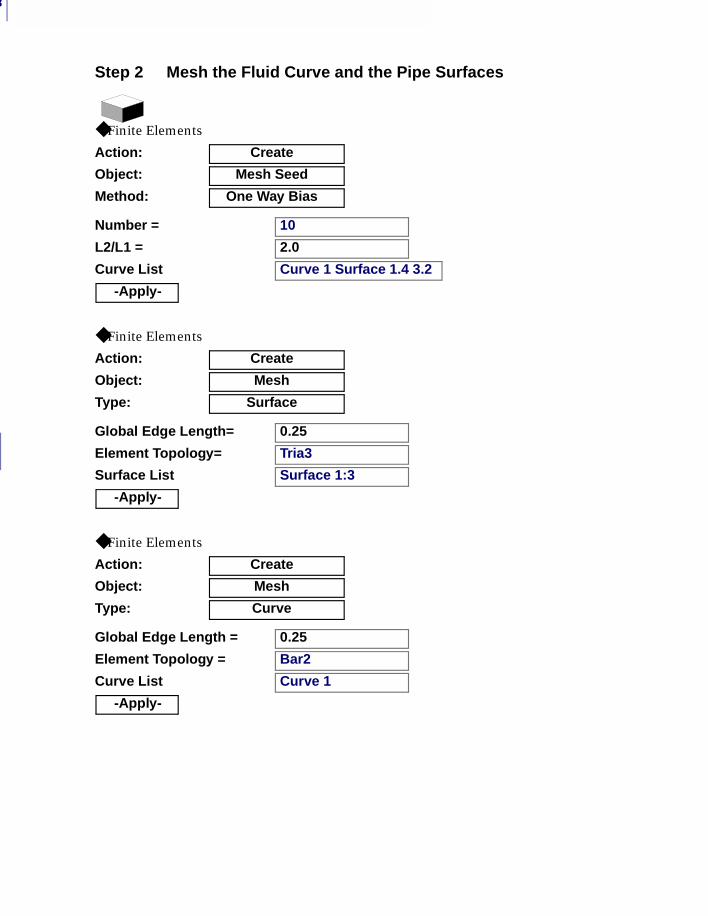
7
228
Step 2 Mesh the Fluid Curve and the Pipe Surfaces
◆ Finite Elements
Action: Create
Object: Mesh Seed
Method: One Way Bias
Number = 10
L2/L1 = 2.0
Curve List Curve 1 Surface 1.4 3.2
-Apply-
◆ Finite Elements
Action: Create
Object: Mesh
Type: Surface
Global Edge Length= 0.25
Element Topology= Tria3
Surface List Surface 1:3
-Apply-
◆ Finite Elements
Action: Create
Object: Mesh
Type: Curve
Global Edge Length = 0.25
Element Topology = Bar2
Curve List Curve 1
-Apply-
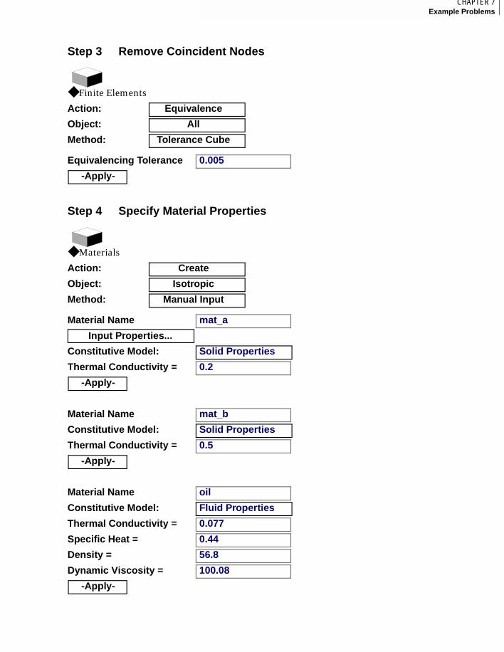
229CHAPTER 7Example Problems
7
Step 3 Remove Coincident Nodes
◆ Finite Elements
Action: Equivalence
Object: All
Method: Tolerance Cube
Equivalencing Tolerance 0.005
-Apply-
Step 4 Specify Material Properties
◆ Materials
Action: Create
Object: Isotropic
Method: Manual Input
Material Name mat_a
Input Properties...
Constitutive Model: Solid Properties
Thermal Conductivity = 0.2
-Apply-
Material Name mat_b
Constitutive Model: Solid Properties
Thermal Conductivity = 0.5
-Apply-
Material Name oil
Constitutive Model: Fluid Properties
Thermal Conductivity = 0.077
Specific Heat = 0.44
Density = 56.8
Dynamic Viscosity = 100.08
-Apply-
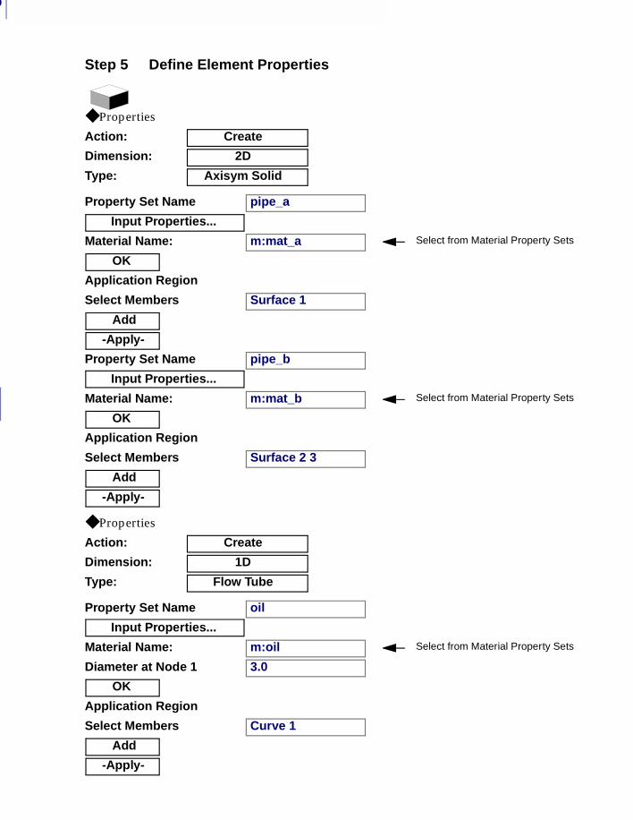
7
230
Step 5 Define Element Properties
◆ Properties
Action: Create
Dimension: 2D
Type: Axisym Solid
Property Set Name pipe_a
Input Properties...
Material Name: m:mat_a Select from Material Property Sets
OK
Application Region
Select Members Surface 1
Add
-Apply-
Property Set Name pipe_b
Input Properties...
Material Name: m:mat_b Select from Material Property Sets
OK
Application Region
Select Members Surface 2 3
Add
-Apply-
◆ Properties
Action: Create
Dimension: 1D
Type: Flow Tube
Property Set Name oil
Input Properties...
Material Name: m:oil Select from Material Property Sets
Diameter at Node 1 3.0
OK
Application Region
Select Members Curve 1
Add
-Apply-
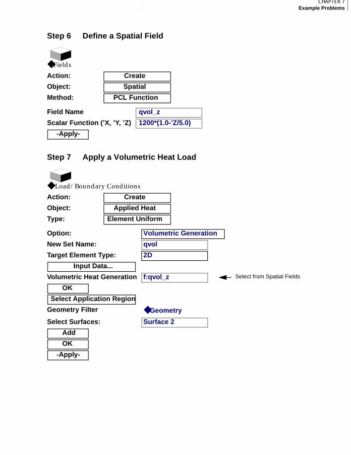
231CHAPTER 7Example Problems
7
Step 6 Define a Spatial Field
◆ Fields
Action: Create
Object: Spatial
Method: PCL Function
Field Name qvol_z
Scalar Function (’X, ’Y, ’Z) 1200*(1.0-’Z/5.0)
-Apply-
Step 7 Apply a Volumetric Heat Load
◆ Load/Boundary Conditions
Action: Create
Object: Applied Heat
Type: Element Uniform
Option: Volumetric Generation
New Set Name: qvol
Target Element Type: 2D
Input Data...
Volumetric Heat Generation f:qvol_z Select from Spatial Fields
OK
Select Application Region
Geometry Filter ◆ Geometry
Select Surfaces: Surface 2
Add
OK
-Apply-
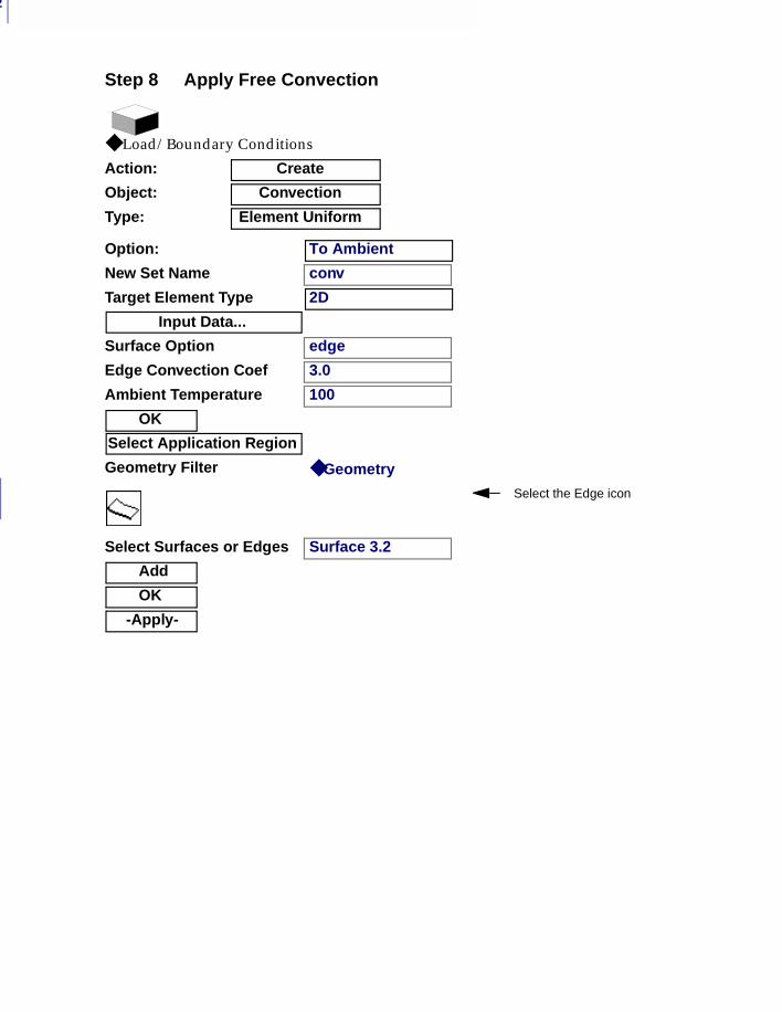
7
232
Step 8 Apply Free Convection
◆ Load/Boundary Conditions
Action: Create
Object: Convection
Type: Element Uniform
Option: To Ambient
New Set Name conv
Target Element Type 2D
Input Data...
Surface Option edge
Edge Convection Coef 3.0
Ambient Temperature 100
OK
Select Application Region
Geometry Filter ◆ Geometry
Select the Edge icon
Select Surfaces or Edges Surface 3.2
Add
OK
-Apply-
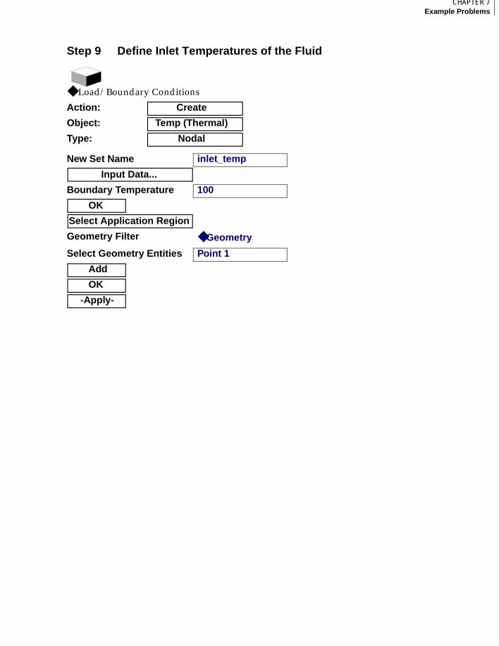
233CHAPTER 7Example Problems
7
Step 9 Define Inlet Temperatures of the Fluid
◆ Load/Boundary Conditions
Action: Create
Object: Temp (Thermal)
Type: Nodal
New Set Name inlet_temp
Input Data...
Boundary Temperature 100
OK
Select Application Region
Geometry Filter ◆ Geometry
Select Geometry Entities Point 1
Add
OK
-Apply-
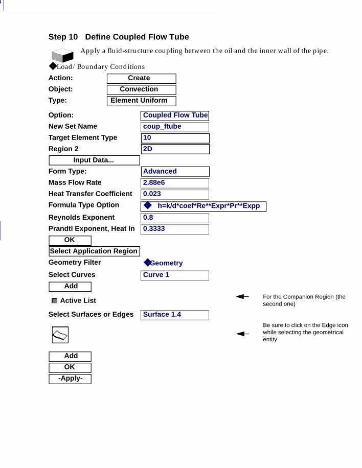
7
234
Step 10 Define Coupled Flow Tube
Apply a fluid-structure coupling between the oil and the inner wall of the pipe.
◆ Load/Boundary Conditions
Action: Create
Object: Convection
Type: Element Uniform
Option: Coupled Flow Tube
New Set Name coup_ftube
Target Element Type 10
Region 2 2D
Input Data...
Form Type: Advanced
Mass Flow Rate 2.88e6
Heat Transfer Coefficient 0.023
Formula Type Option ◆ h=k/d*coef*Re**Expr*Pr**Expp
Reynolds Exponent 0.8
Prandtl Exponent, Heat In 0.3333
OK
Select Application Region
Geometry Filter ◆ Geometry
Select Curves Curve 1
Add
Active List For the Companion Region (the second one)
Select Surfaces or Edges Surface 1.4Be sure to click on the Edge iconwhile selecting the geometrical entity
Add
OK
-Apply-
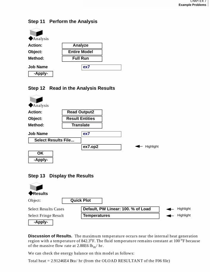
235CHAPTER 7Example Problems
7
Discussion of Results. The maximum temperature occurs near the internal heat generation region with a temperature of 842.3oF. The fluid temperature remains constant at 100 oF because of the massive flow rate at 2.88E6 lbm/hr.
We can check the energy balance on this model as follows:
Total heat = 2.91246E4 Btu/hr (from the OLOAD RESULTANT of the F06 file)
Step 11 Perform the Analysis
◆ Analysis
Action: Analyze
Object: Entire Model
Method: Full Run
Job Name ex7
-Apply-
Step 12 Read in the Analysis Results
◆ Analysis
Action: Read Output2
Object: Result Entities
Method: Translate
Job Name ex7
Select Results File...
ex7.op2 Highlight
OK
-Apply-
Step 13 Display the Results
◆ Results
Object: Quick Plot
Select Results Cases Default, PW Linear: 100. % of Load Highlight
Select Fringe Result Temperatures Highlight
-Apply-

7
236
Sum of the heat on the column under Free Convection = 2.5828E4 Btu/hr
Sum of the heat on the column under Forced Convection = 3.297E3 Btu/hr
Sum of the heat on the above two columns = 2.9125E4 Btu/hr, which is equal to the input heat of 2.91246E4 Btu/hr.
An assumption of a 1-D fluid element is that temperature gradients within the fluid are only significant along the axial direction. With such a large diameter flow tube, this assumption is probably being misused in this particular problem. The application of the flow tube boundary convection relationship also implies fully developed flow, yet, over only a 5 foot section and with a 3 foot diameter, this is also a very crude approximation. In essence, what we are saying, is that this example serves to illustrate coupled convection in an axisymmetric environment, application of spatial heat loads, and use of convection correlation equations, rather than fluid physics.
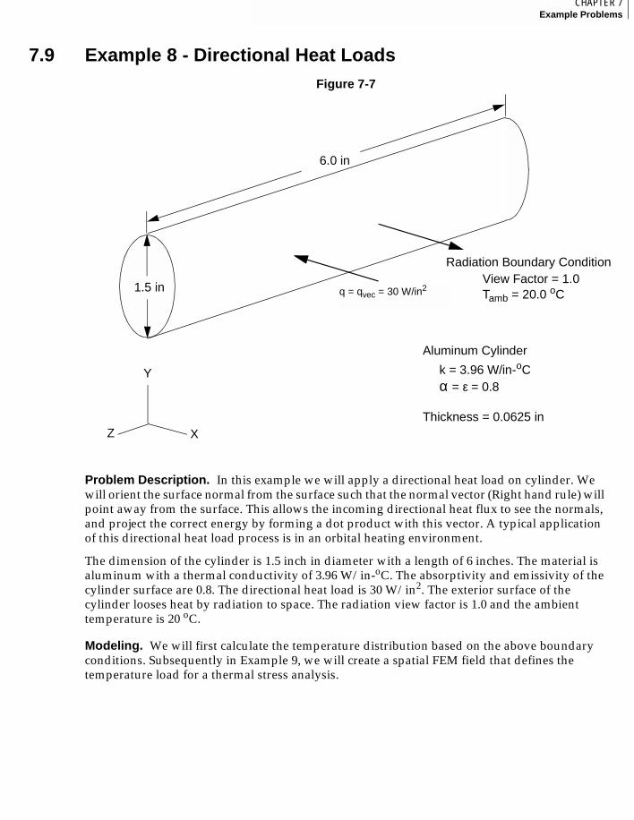
237CHAPTER 7Example Problems
7
7.9 Example 8 - Directional Heat LoadsFigure 7-7
Problem Description. In this example we will apply a directional heat load on cylinder. We will orient the surface normal from the surface such that the normal vector (Right hand rule) will point away from the surface. This allows the incoming directional heat flux to see the normals, and project the correct energy by forming a dot product with this vector. A typical application of this directional heat load process is in an orbital heating environment.
The dimension of the cylinder is 1.5 inch in diameter with a length of 6 inches. The material is aluminum with a thermal conductivity of 3.96 W/in-oC. The absorptivity and emissivity of the cylinder surface are 0.8. The directional heat load is 30 W/in2. The exterior surface of the cylinder looses heat by radiation to space. The radiation view factor is 1.0 and the ambient temperature is 20 oC.
Modeling. We will first calculate the temperature distribution based on the above boundary conditions. Subsequently in Example 9, we will create a spatial FEM field that defines the temperature load for a thermal stress analysis.
6.0 in
q = qvec = 30 W/in2Tamb = 20.0 oCView Factor = 1.0
1.5 in
k = 3.96 W/in-oC
Aluminum Cylinder
α = ε = 0.8
Thickness = 0.0625 in
Radiation Boundary Condition
X
Y
Z
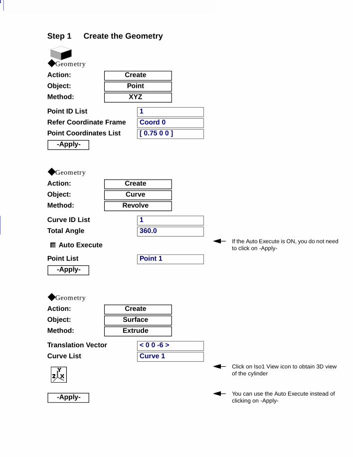
7
238
Step 1 Create the Geometry
◆ Geometry
Action: Create
Object: Point
Method: XYZ
Point ID List 1
Refer Coordinate Frame Coord 0
Point Coordinates List [ 0.75 0 0 ]
-Apply-
◆ Geometry
Action: Create
Object: Curve
Method: Revolve
Curve ID List 1
Total Angle 360.0
Auto Execute If the Auto Execute is ON, you do not needto click on -Apply-
Point List Point 1
-Apply-
◆ Geometry
Action: Create
Object: Surface
Method: Extrude
Translation Vector < 0 0 -6 >
Curve List Curve 1Click on Iso1 View icon to obtain 3D view of the cylinder
-Apply- You can use the Auto Execute instead of clicking on -Apply-
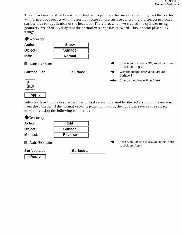
239CHAPTER 7Example Problems
7
The surface normal direction is important in this problem, because the incoming heat flux vector will form a dot product with the normal vector for the surface generating the correct projected surface area for application of the heat load. Therefore, when we created the cylinder using geometry, we should verify that the normal vector points outward. This is accomplished by using:
Select Surface 1 to make sure that the normal vector indicated by the red arrow points outward from the cylinder. If the normal vector is pointing inward, then you can reverse the surface normal by using the following command:
◆ Geometry
Action: Show
Object: Surface
Info: Normal
Auto Execute If the Auto Execute is ON, you do not needto click on -Apply-
Surface List Surface 1 With the mouse draw a box around Surface 1
Change the view to Front View
-Apply-
◆ Geometry
Action: Edit
Object: Surface
Method: Reverse
Auto Execute If the Auto Execute is ON, you do not needto click on -Apply-
Surface List Surface 1
-Apply-
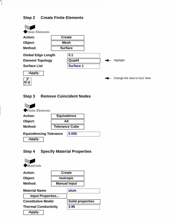
7
240
Step 2 Create Finite Elements
◆ Finite Elements
Action: Create
Object: Mesh
Method: Surface
Global Edge Length 0.1
Element Topology Quad4 Highlight
Surface List Surface 1
-Apply-Change the view to Iso1 View
Step 3 Remove Coincident Nodes
◆ Finite Elements
Action: Equivalence
Object: All
Method: Tolerance Cube
Equivalencing Tolerance 0.005
-Apply-
Step 4 Specify Material Properties
◆ Materials
Action: Create
Object: Isotropic
Method: Manual Input
Material Name alum
Input Properties...
Constitutive Model Solid properties
Thermal Conductivity 3.96
-Apply-
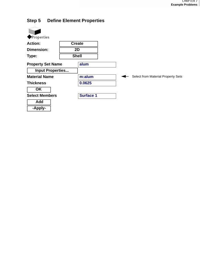
241CHAPTER 7Example Problems
7
Step 5 Define Element Properties
◆ Properties
Action: Create
Dimension: 2D
Type: Shell
Property Set Name alum
Input Properties...
Material Name m:alum Select from Material Property Sets
Thickness 0.0625
OK
Select Members Surface 1
Add
-Apply-
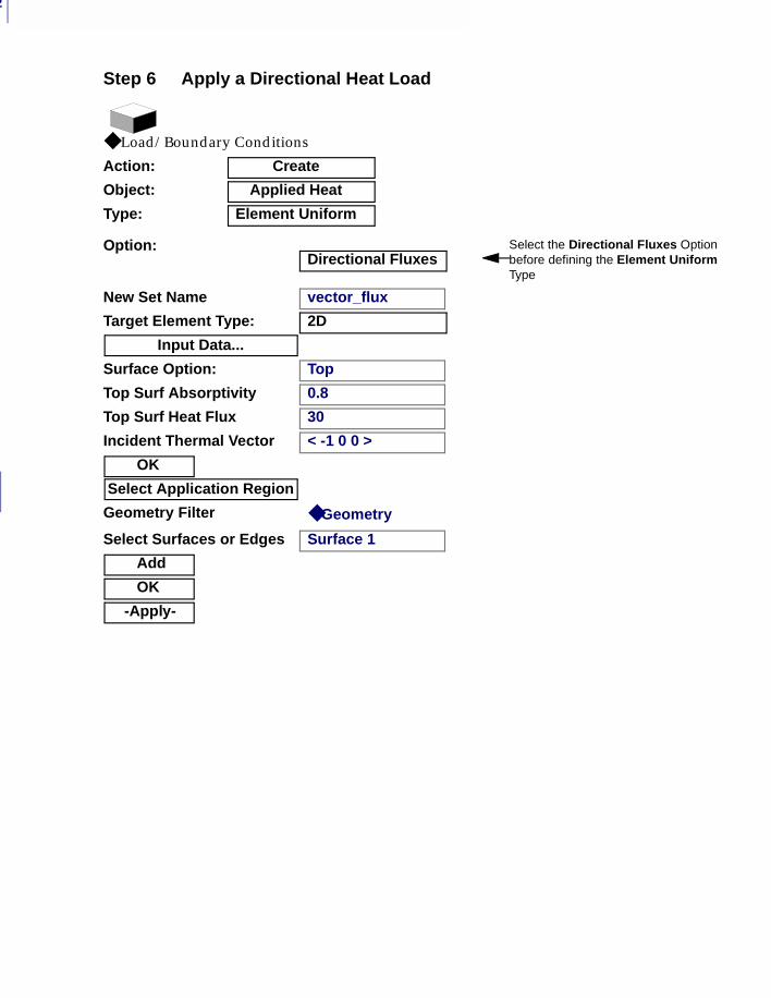
7
242
Step 6 Apply a Directional Heat Load
◆ Load/Boundary Conditions
Action: Create
Object: Applied Heat
Type: Element Uniform
Option:Directional Fluxes
Select the Directional Fluxes Option before defining the Element Uniform Type
New Set Name vector_flux
Target Element Type: 2D
Input Data...
Surface Option: Top
Top Surf Absorptivity 0.8
Top Surf Heat Flux 30
Incident Thermal Vector < -1 0 0 >
OK
Select Application Region
Geometry Filter ◆ Geometry
Select Surfaces or Edges Surface 1
Add
OK
-Apply-
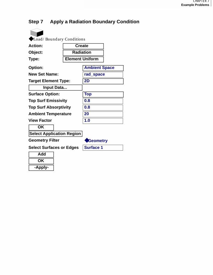
243CHAPTER 7Example Problems
7
Step 7 Apply a Radiation Boundary Condition
◆ Load/Boundary Conditions
Action: Create
Object: Radiation
Type: Element Uniform
Option: Ambient Space
New Set Name: rad_space
Target Element Type: 2D
Input Data...
Surface Option: Top
Top Surf Emissivity 0.8
Top Surf Absorptivity 0.8
Ambient Temperature 20
View Factor 1.0
OK
Select Application Region
Geometry Filter ◆ Geometry
Select Surfaces or Edges Surface 1
Add
OK
-Apply-

7
244
Step 8 Specify Radiation Parameters and Perform the Analysis
◆ Analysis
Action: Analyze
Object: Entire Model
Method: Full Run
Job Name ex8
Solution Type...
STEADY STATE ANALYSIS
Solution Parameters...
Radiation Parameters...
Absolute Temperature Scale: 273.15 Click on Absolute Temperature Scale for list in various units
Stefan-Boltzmann Constant: 3.6580E-11 Click on Stefan-Boltzmann Constant for list in various units
OK
OK
OK
-Apply-
Step 9 Read in the Analysis Results
◆ Analysis
Action: Read Output2
Object: Result Entities
Method: Translate
Job Name ex8
Select Results File... ex8.op2 Highlight
OK
-Apply-
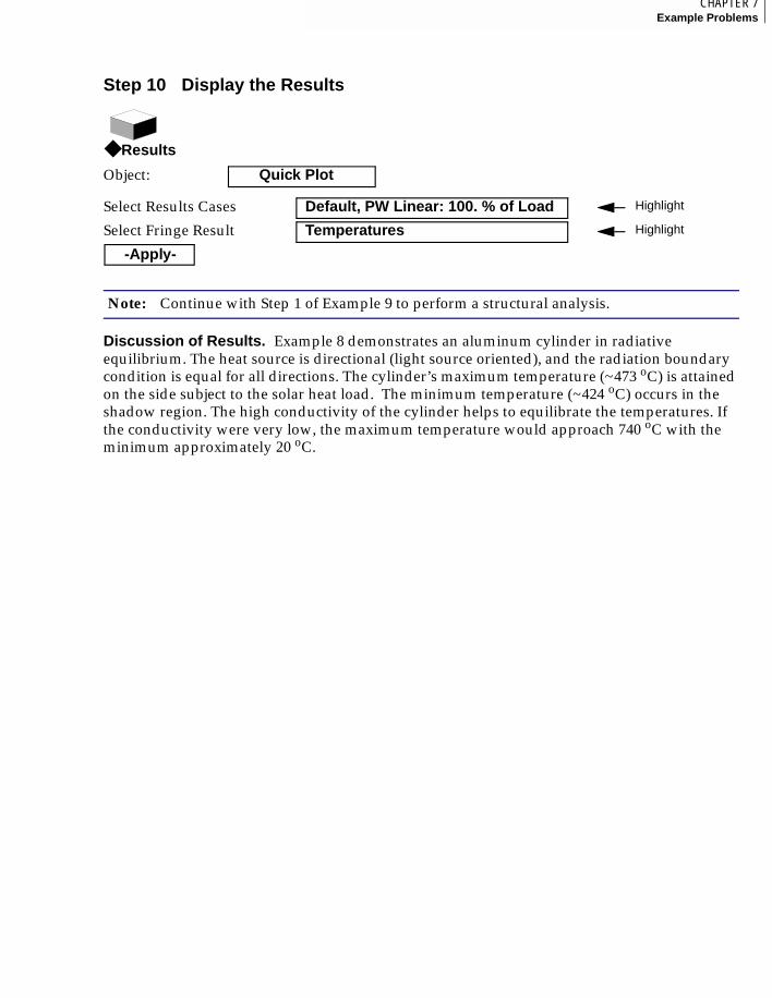
245CHAPTER 7Example Problems
7
Discussion of Results. Example 8 demonstrates an aluminum cylinder in radiative equilibrium. The heat source is directional (light source oriented), and the radiation boundary condition is equal for all directions. The cylinder’s maximum temperature (~473 oC) is attained on the side subject to the solar heat load. The minimum temperature (~424 oC) occurs in the shadow region. The high conductivity of the cylinder helps to equilibrate the temperatures. If the conductivity were very low, the maximum temperature would approach 740 oC with the minimum approximately 20 oC.
Note: Continue with Step 1 of Example 9 to perform a structural analysis.
Step 10 Display the Results
◆ Results
Object: Quick Plot
Select Results Cases Default, PW Linear: 100. % of Load Highlight
Select Fringe Result Temperatures Highlight
-Apply-
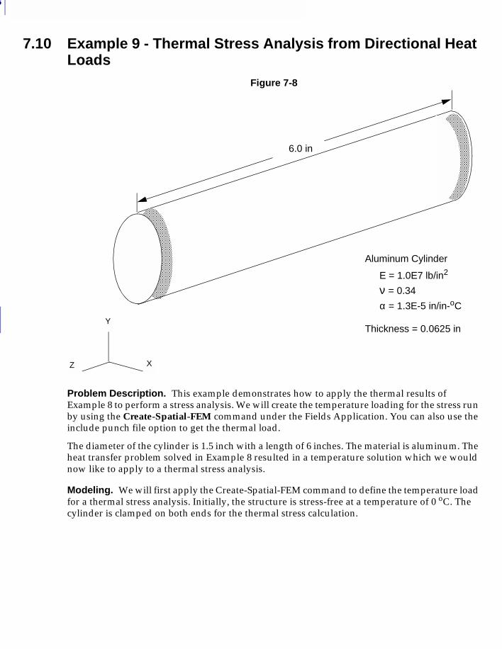
7
246
7.10 Example 9 - Thermal Stress Analysis from Directional Heat Loads
Figure 7-8
Problem Description. This example demonstrates how to apply the thermal results of Example 8 to perform a stress analysis. We will create the temperature loading for the stress run by using the Create-Spatial-FEM command under the Fields Application. You can also use the include punch file option to get the thermal load.
The diameter of the cylinder is 1.5 inch with a length of 6 inches. The material is aluminum. The heat transfer problem solved in Example 8 resulted in a temperature solution which we would now like to apply to a thermal stress analysis.
Modeling. We will first apply the Create-Spatial-FEM command to define the temperature load for a thermal stress analysis. Initially, the structure is stress-free at a temperature of 0 oC. The cylinder is clamped on both ends for the thermal stress calculation.
6.0 in
Y
XZ
1.5 in
E = 1.0E7 lb/in2
Aluminum Cylinder
ν = 0.34
Thickness = 0.0625 in
α = 1.3E-5 in/in-oC
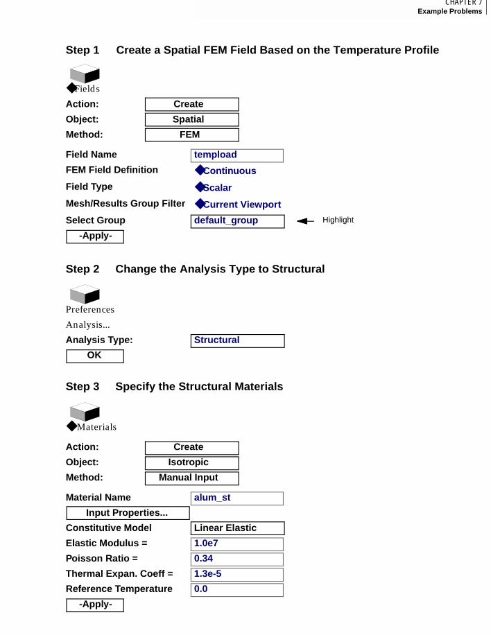
247CHAPTER 7Example Problems
7
Step 1 Create a Spatial FEM Field Based on the Temperature Profile
◆ Fields
Action: Create
Object: Spatial
Method: FEM
Field Name tempload
FEM Field Definition ◆ Continuous
Field Type ◆ Scalar
Mesh/Results Group Filter ◆ Current Viewport
Select Group default_group Highlight
-Apply-
Step 2 Change the Analysis Type to Structural
Preferences
Analysis...
Analysis Type: Structural
OK
Step 3 Specify the Structural Materials
◆ Materials
Action: Create
Object: Isotropic
Method: Manual Input
Material Name alum_st
Input Properties...
Constitutive Model Linear Elastic
Elastic Modulus = 1.0e7
Poisson Ratio = 0.34
Thermal Expan. Coeff = 1.3e-5
Reference Temperature 0.0
-Apply-
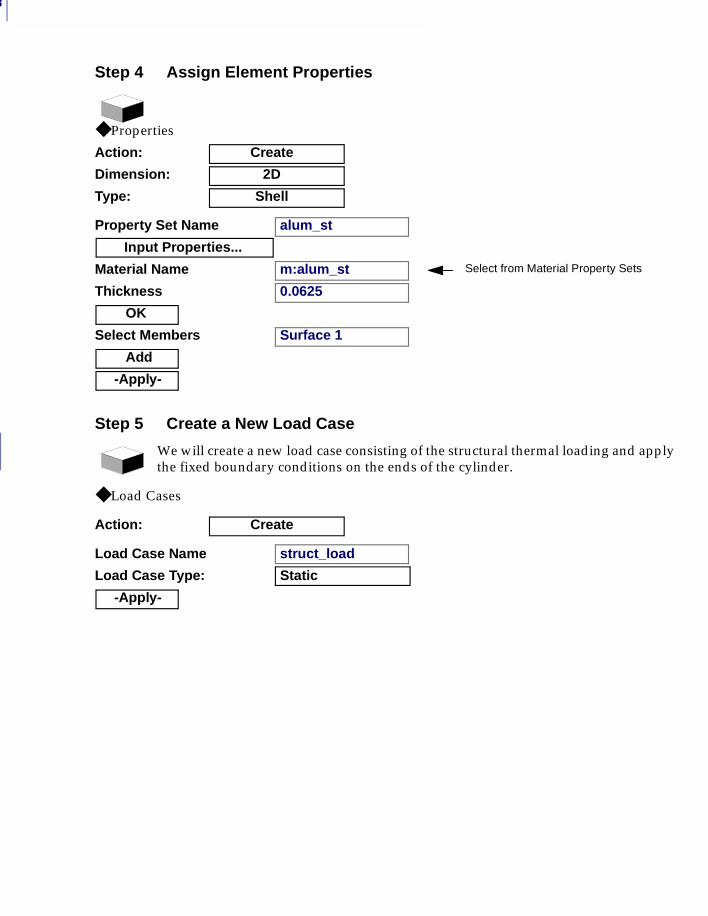
7
248
Step 4 Assign Element Properties
◆ Properties
Action: Create
Dimension: 2D
Type: Shell
Property Set Name alum_st
Input Properties...
Material Name m:alum_st Select from Material Property Sets
Thickness 0.0625
OK
Select Members Surface 1
Add
-Apply-
Step 5 Create a New Load Case
We will create a new load case consisting of the structural thermal loading and apply the fixed boundary conditions on the ends of the cylinder.
◆ Load Cases
Action: Create
Load Case Name struct_load
Load Case Type: Static
-Apply-
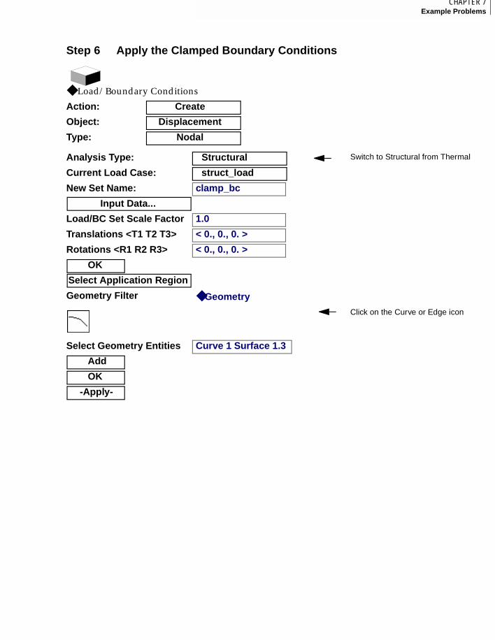
249CHAPTER 7Example Problems
7
Step 6 Apply the Clamped Boundary Conditions
◆ Load/Boundary Conditions
Action: Create
Object: Displacement
Type: Nodal
Analysis Type: Structural Switch to Structural from Thermal
Current Load Case: struct_load
New Set Name: clamp_bc
Input Data...
Load/BC Set Scale Factor 1.0
Translations <T1 T2 T3> < 0., 0., 0. >
Rotations <R1 R2 R3> < 0., 0., 0. >
OK
Select Application Region
Geometry Filter ◆ Geometry
Click on the Curve or Edge icon
Select Geometry Entities Curve 1 Surface 1.3
Add
OK
-Apply-
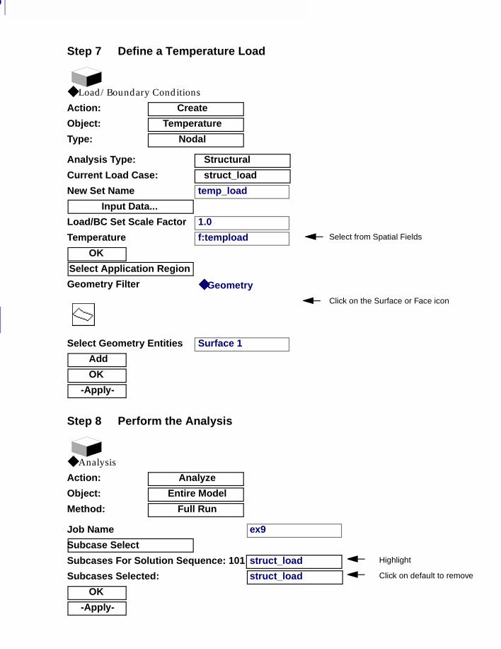
7
250
Step 7 Define a Temperature Load
◆ Load/Boundary Conditions
Action: Create
Object: Temperature
Type: Nodal
Analysis Type: Structural
Current Load Case: struct_load
New Set Name temp_load
Input Data...
Load/BC Set Scale Factor 1.0
Temperature f:tempload Select from Spatial Fields
OK
Select Application Region
Geometry Filter ◆ Geometry
Click on the Surface or Face icon
Select Geometry Entities Surface 1
Add
OK
-Apply-
Step 8 Perform the Analysis
◆ Analysis
Action: Analyze
Object: Entire Model
Method: Full Run
Job Name ex9
Subcase Select
Subcases For Solution Sequence: 101 struct_load Highlight
Subcases Selected: struct_load Click on default to remove
OK
-Apply-
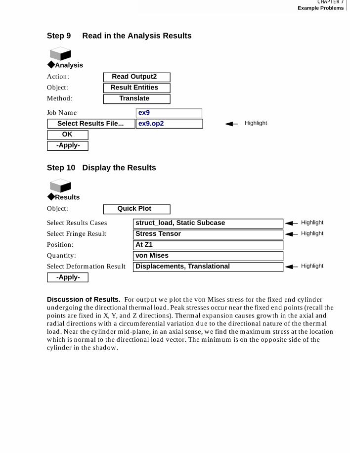
251CHAPTER 7Example Problems
7
Discussion of Results. For output we plot the von Mises stress for the fixed end cylinder undergoing the directional thermal load. Peak stresses occur near the fixed end points (recall the points are fixed in X, Y, and Z directions). Thermal expansion causes growth in the axial and radial directions with a circumferential variation due to the directional nature of the thermal load. Near the cylinder mid-plane, in an axial sense, we find the maximum stress at the location which is normal to the directional load vector. The minimum is on the opposite side of the cylinder in the shadow.
Step 9 Read in the Analysis Results
◆ Analysis
Action: Read Output2
Object: Result Entities
Method: Translate
Job Name ex9
Select Results File... ex9.op2 Highlight
OK
-Apply-
Step 10 Display the Results
◆ Results
Object: Quick Plot
Select Results Cases struct_load, Static Subcase Highlight
Select Fringe Result Stress Tensor Highlight
Position: At Z1
Quantity: von Mises
Select Deformation Result Displacements, Translational Highlight
-Apply-
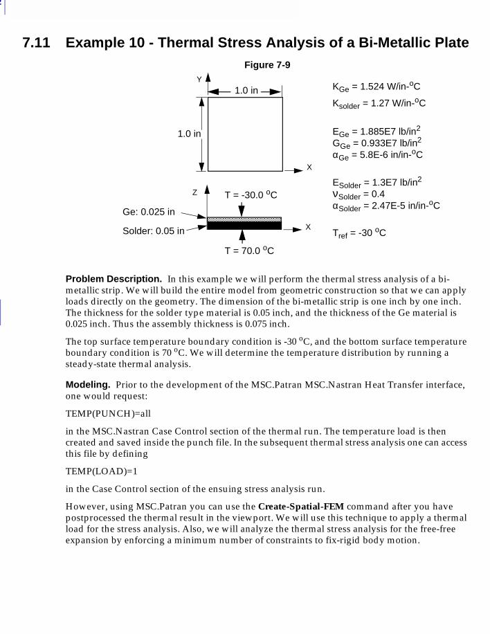
7
252
7.11 Example 10 - Thermal Stress Analysis of a Bi-Metallic PlateFigure 7-9
Problem Description. In this example we will perform the thermal stress analysis of a bi-metallic strip. We will build the entire model from geometric construction so that we can apply loads directly on the geometry. The dimension of the bi-metallic strip is one inch by one inch. The thickness for the solder type material is 0.05 inch, and the thickness of the Ge material is 0.025 inch. Thus the assembly thickness is 0.075 inch.
The top surface temperature boundary condition is -30 oC, and the bottom surface temperature boundary condition is 70 oC. We will determine the temperature distribution by running a steady-state thermal analysis.
Modeling. Prior to the development of the MSC.Patran MSC.Nastran Heat Transfer interface, one would request:
TEMP(PUNCH)=all
in the MSC.Nastran Case Control section of the thermal run. The temperature load is then created and saved inside the punch file. In the subsequent thermal stress analysis one can access this file by defining
TEMP(LOAD)=1
in the Case Control section of the ensuing stress analysis run.
However, using MSC.Patran you can use the Create-Spatial-FEM command after you have postprocessed the thermal result in the viewport. We will use this technique to apply a thermal load for the stress analysis. Also, we will analyze the thermal stress analysis for the free-free expansion by enforcing a minimum number of constraints to fix-rigid body motion.
T = 70.0 oC
KGe = 1.524 W/in-oC
Ksolder = 1.27 W/in-oC
X
Y
1.0 in
1.0 in
X
Ge: 0.025 in
Solder: 0.05 in
Z T = -30.0 oC
EGe = 1.885E7 lb/in2
GGe = 0.933E7 lb/in2
αGe = 5.8E-6 in/in-oC
ESolder = 1.3E7 lb/in2
νSolder = 0.4αSolder = 2.47E-5 in/in-oC
Tref = -30 oC
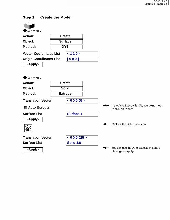
253CHAPTER 7Example Problems
7
Step 1 Create the Model
◆ Geometry
Action: Create
Object: Surface
Method: XYZ
Vector Coordinates List < 1 1 0 >
Origin Coordinates List [ 0 0 0 ]
-Apply-
◆ Geometry
Action: Create
Object: Solid
Method: Extrude
Translation Vector < 0 0 0.05 >
Auto ExecuteIf the Auto Execute is ON, you do not needto click on -Apply-
Surface List Surface 1
-Apply-Click on the Solid Face icon
Translation Vector < 0 0 0.025 >
Surface List Solid 1.6
-Apply- You can use the Auto Execute instead of clicking on -Apply-
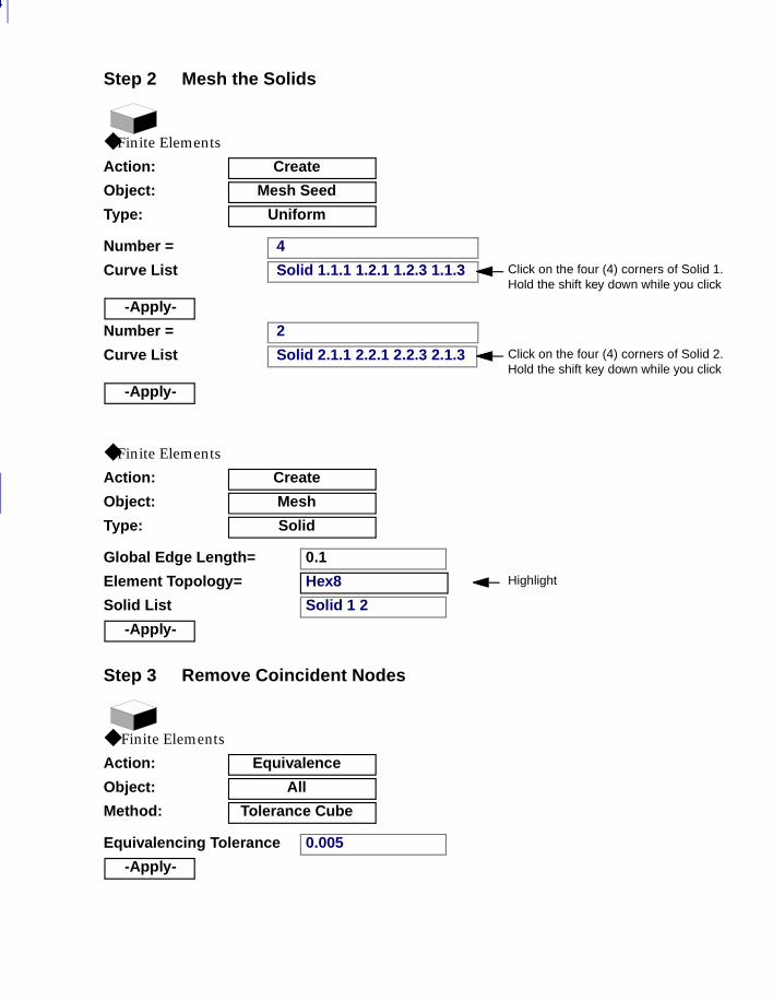
7
254
Step 2 Mesh the Solids
◆ Finite Elements
Action: Create
Object: Mesh Seed
Type: Uniform
Number = 4
Curve List Solid 1.1.1 1.2.1 1.2.3 1.1.3 Click on the four (4) corners of Solid 1. Hold the shift key down while you click
-Apply-
Number = 2
Curve List Solid 2.1.1 2.2.1 2.2.3 2.1.3 Click on the four (4) corners of Solid 2. Hold the shift key down while you click
-Apply-
◆ Finite Elements
Action: Create
Object: Mesh
Type: Solid
Global Edge Length= 0.1
Element Topology= Hex8 Highlight
Solid List Solid 1 2
-Apply-
Step 3 Remove Coincident Nodes
◆ Finite Elements
Action: Equivalence
Object: All
Method: Tolerance Cube
Equivalencing Tolerance 0.005
-Apply-
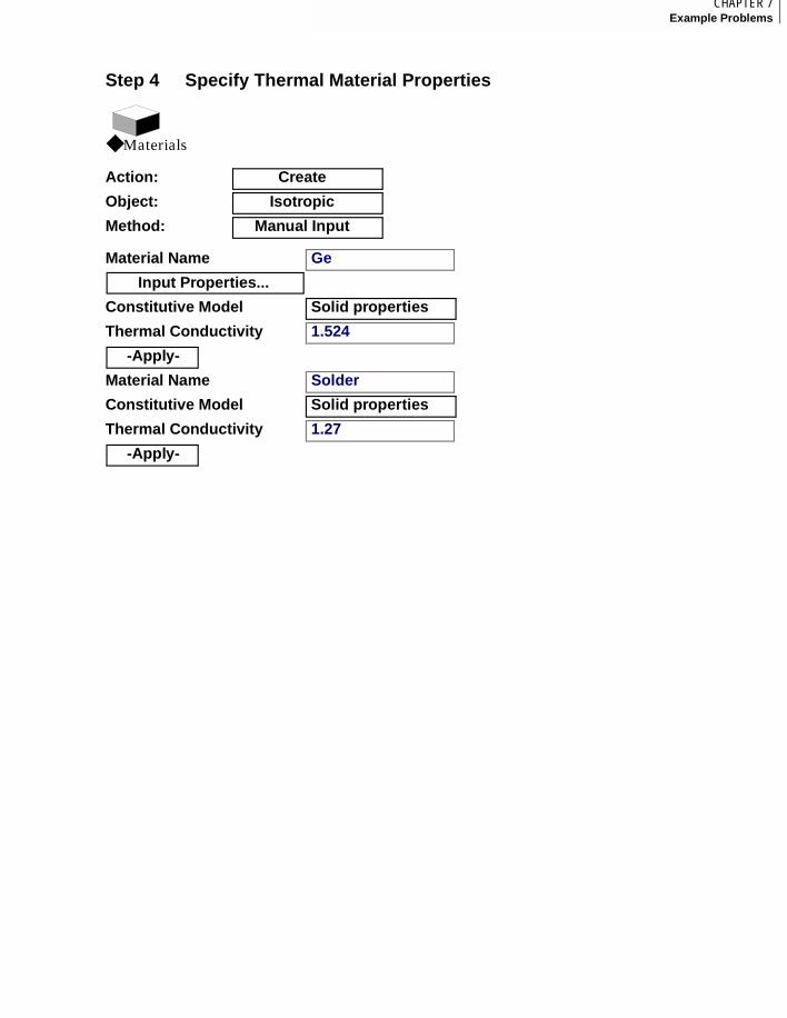
255CHAPTER 7Example Problems
7
Step 4 Specify Thermal Material Properties
◆ Materials
Action: Create
Object: Isotropic
Method: Manual Input
Material Name Ge
Input Properties...
Constitutive Model Solid properties
Thermal Conductivity 1.524
-Apply-
Material Name Solder
Constitutive Model Solid properties
Thermal Conductivity 1.27
-Apply-
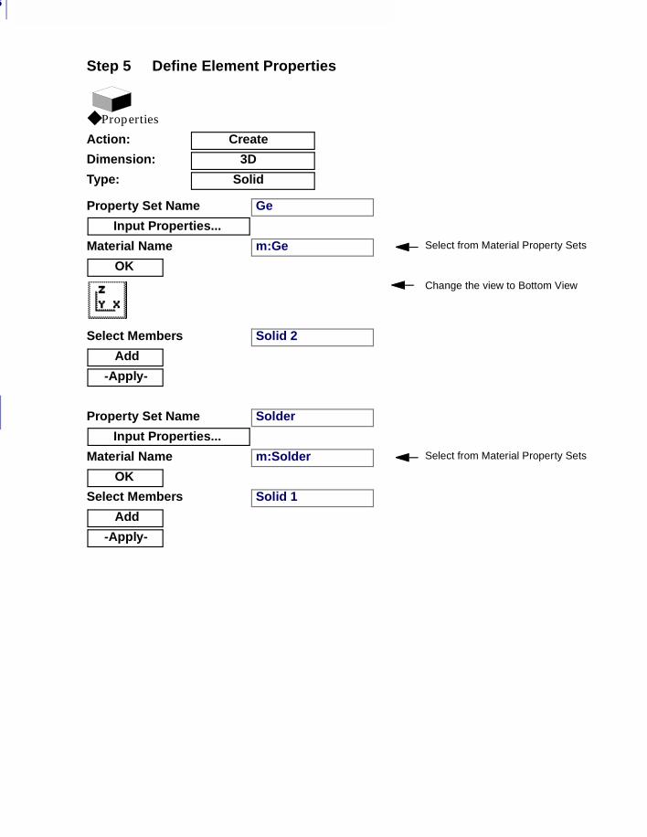
7
256
Step 5 Define Element Properties
◆ Properties
Action: Create
Dimension: 3D
Type: Solid
Property Set Name Ge
Input Properties...
Material Name m:Ge Select from Material Property Sets
OKChange the view to Bottom View
Select Members Solid 2
Add
-Apply-
Property Set Name Solder
Input Properties...
Material Name m:Solder Select from Material Property Sets
OK
Select Members Solid 1
Add
-Apply-
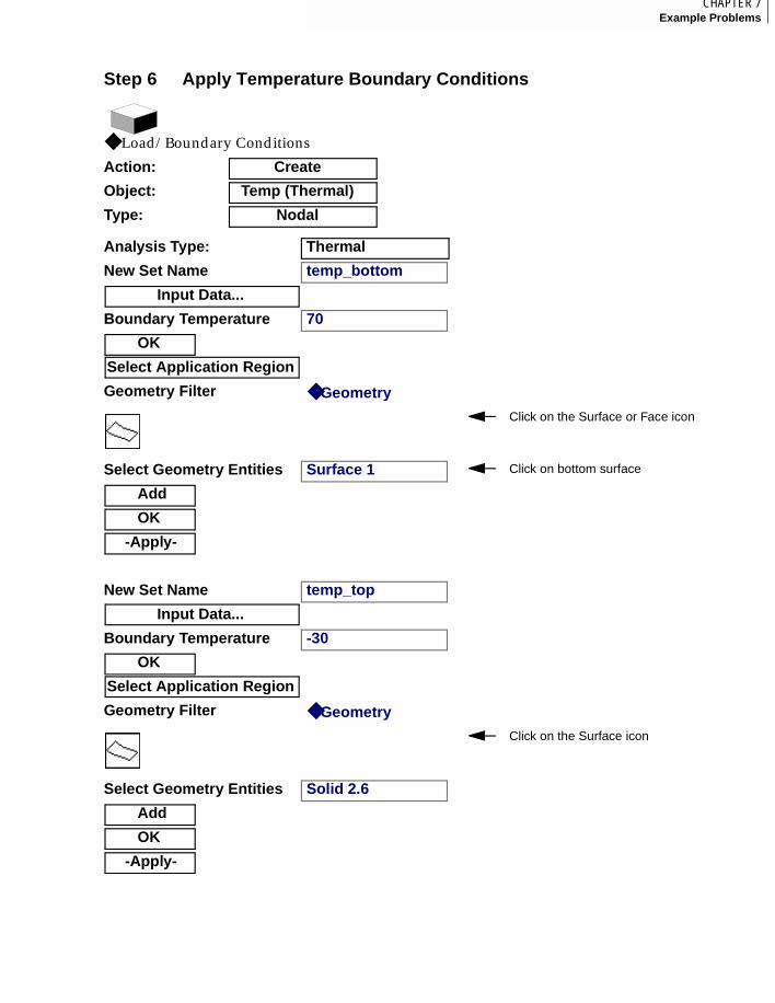
257CHAPTER 7Example Problems
7
Step 6 Apply Temperature Boundary Conditions
◆ Load/Boundary Conditions
Action: Create
Object: Temp (Thermal)
Type: Nodal
Analysis Type: Thermal
New Set Name temp_bottom
Input Data...
Boundary Temperature 70
OK
Select Application Region
Geometry Filter ◆ Geometry
Click on the Surface or Face icon
Select Geometry Entities Surface 1 Click on bottom surface
Add
OK
-Apply-
New Set Name temp_top
Input Data...
Boundary Temperature -30
OK
Select Application Region
Geometry Filter ◆ Geometry
Click on the Surface icon
Select Geometry Entities Solid 2.6
Add
OK
-Apply-
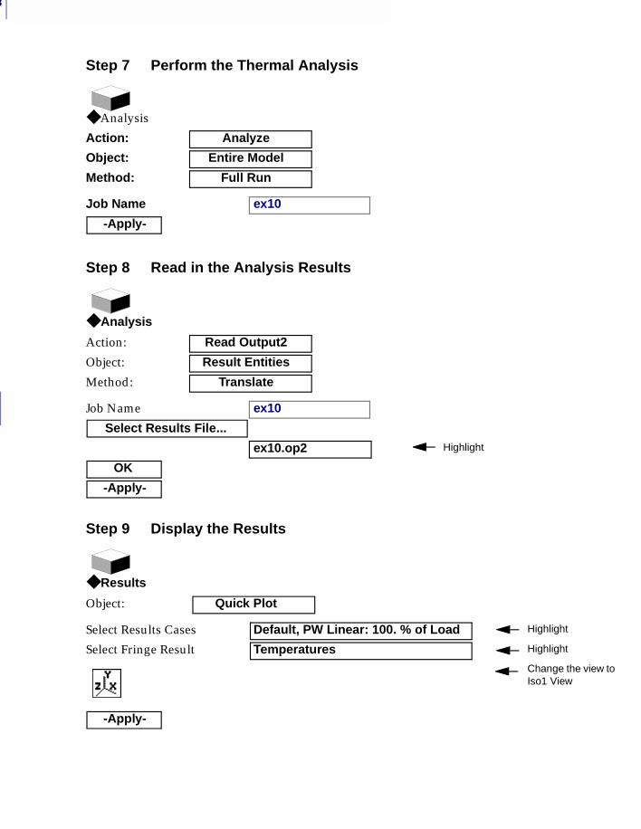
7
258
Step 7 Perform the Thermal Analysis
◆ Analysis
Action: Analyze
Object: Entire Model
Method: Full Run
Job Name ex10
-Apply-
Step 8 Read in the Analysis Results
◆ Analysis
Action: Read Output2
Object: Result Entities
Method: Translate
Job Name ex10
Select Results File...
ex10.op2 Highlight
OK
-Apply-
Step 9 Display the Results
◆ Results
Object: Quick Plot
Select Results Cases Default, PW Linear: 100. % of Load Highlight
Select Fringe Result Temperatures Highlight
Change the view toIso1 View
-Apply-
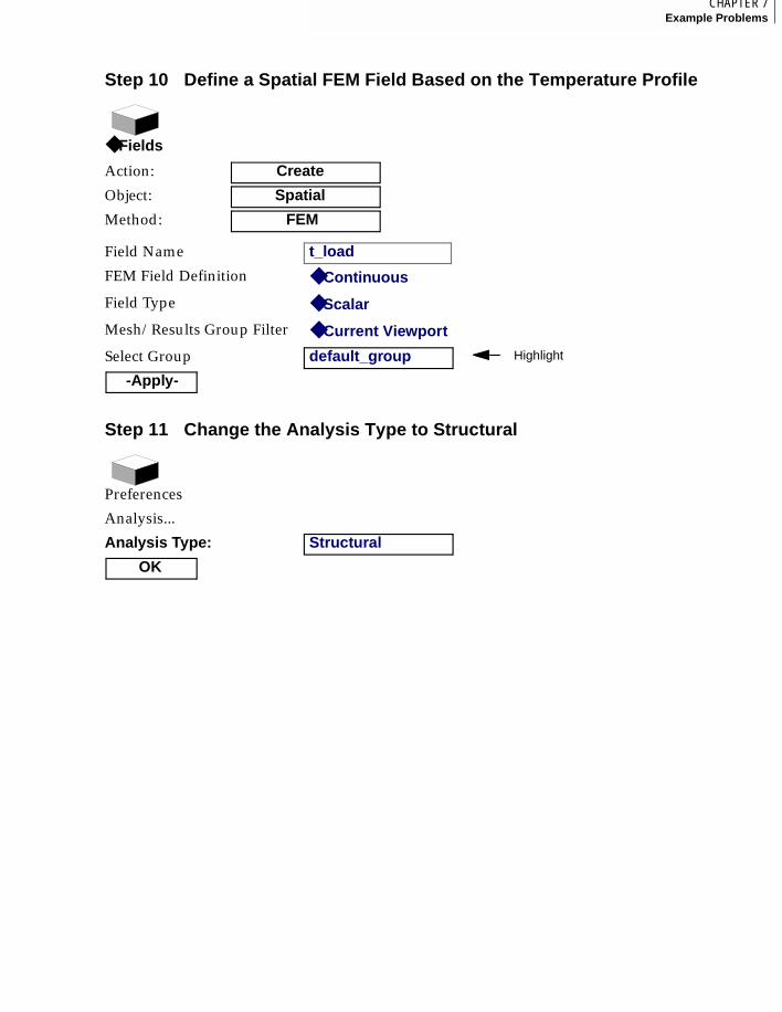
259CHAPTER 7Example Problems
7
Step 10 Define a Spatial FEM Field Based on the Temperature Profile
◆ Fields
Action: Create
Object: Spatial
Method: FEM
Field Name t_load
FEM Field Definition ◆ Continuous
Field Type ◆ Scalar
Mesh/Results Group Filter ◆ Current Viewport
Select Group default_group Highlight
-Apply-
Step 11 Change the Analysis Type to Structural
Preferences
Analysis...
Analysis Type: Structural
OK
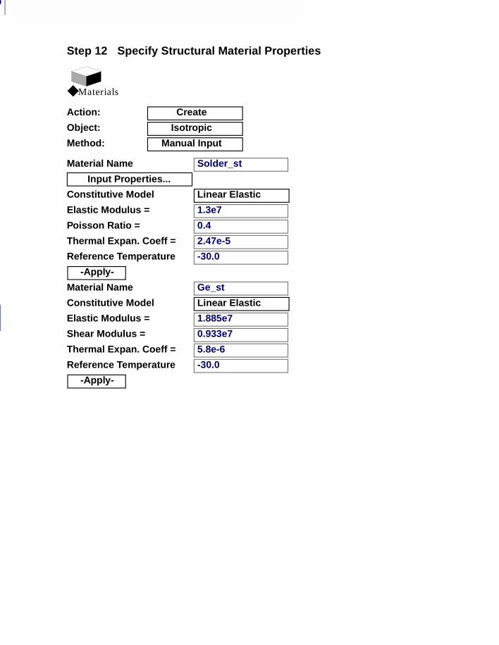
7
260
Step 12 Specify Structural Material Properties
◆ Materials
Action: Create
Object: Isotropic
Method: Manual Input
Material Name Solder_st
Input Properties...
Constitutive Model Linear Elastic
Elastic Modulus = 1.3e7
Poisson Ratio = 0.4
Thermal Expan. Coeff = 2.47e-5
Reference Temperature -30.0
-Apply-
Material Name Ge_st
Constitutive Model Linear Elastic
Elastic Modulus = 1.885e7
Shear Modulus = 0.933e7
Thermal Expan. Coeff = 5.8e-6
Reference Temperature -30.0
-Apply-
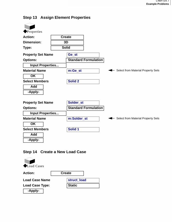
261CHAPTER 7Example Problems
7
Step 13 Assign Element Properties
◆ Properties
Action: Create
Dimension: 3D
Type: Solid
Property Set Name Ge_st
Options: Standard Formulation
Input Properties...
Material Name m:Ge_st Select from Material Property Sets
OK
Select Members Solid 2
Add
-Apply-
Property Set Name Solder_st
Options: Standard Formulation
Input Properties...
Material Name m:Solder_st Select from Material Property Sets
OK
Select Members Solid 1
Add
-Apply-
Step 14 Create a New Load Case
◆ Load Cases
Action: Create
Load Case Name struct_load
Load Case Type: Static
-Apply-
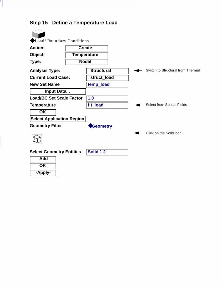
7
262
Step 15 Define a Temperature Load
◆ Load/Boundary Conditions
Action: Create
Object: Temperature
Type: Nodal
Analysis Type: Structural Switch to Structural from Thermal
Current Load Case: struct_load
New Set Name temp_load
Input Data...
Load/BC Set Scale Factor 1.0
Temperature f:t_load Select from Spatial Fields
OK
Select Application Region
Geometry Filter ◆ Geometry
Click on the Solid icon
Select Geometry Entities Solid 1 2
Add
OK
-Apply-
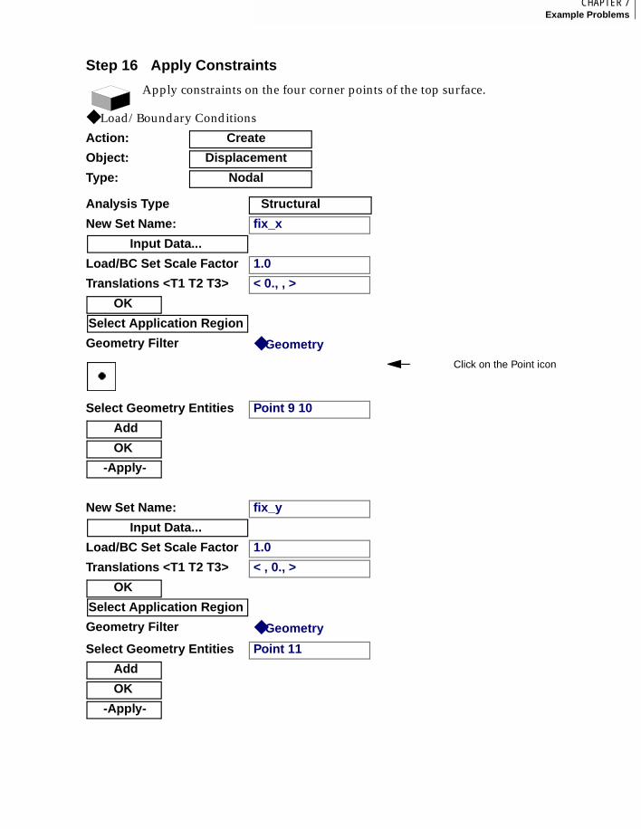
263CHAPTER 7Example Problems
7
Step 16 Apply Constraints
Apply constraints on the four corner points of the top surface.
◆ Load/Boundary Conditions
Action: Create
Object: Displacement
Type: Nodal
Analysis Type Structural
New Set Name: fix_x
Input Data...
Load/BC Set Scale Factor 1.0
Translations <T1 T2 T3> < 0., , >
OK
Select Application Region
Geometry Filter ◆ Geometry
Click on the Point icon
Select Geometry Entities Point 9 10
Add
OK
-Apply-
New Set Name: fix_y
Input Data...
Load/BC Set Scale Factor 1.0
Translations <T1 T2 T3> < , 0., >
OK
Select Application Region
Geometry Filter ◆ Geometry
Select Geometry Entities Point 11
Add
OK
-Apply-
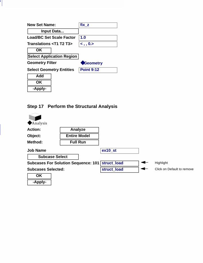
7
264
New Set Name: fix_z
Input Data...
Load/BC Set Scale Factor 1.0
Translations <T1 T2 T3> < , , 0.>
OK
Select Application Region
Geometry Filter ◆ Geometry
Select Geometry Entities Point 9:12
Add
OK
-Apply-
Step 17 Perform the Structural Analysis
◆ Analysis
Action: Analyze
Object: Entire Model
Method: Full Run
Job Name ex10_st
Subcase Select
Subcases For Solution Sequence: 101 struct_load Highlight
Subcases Selected: struct_load Click on Default to remove
OK
-Apply-
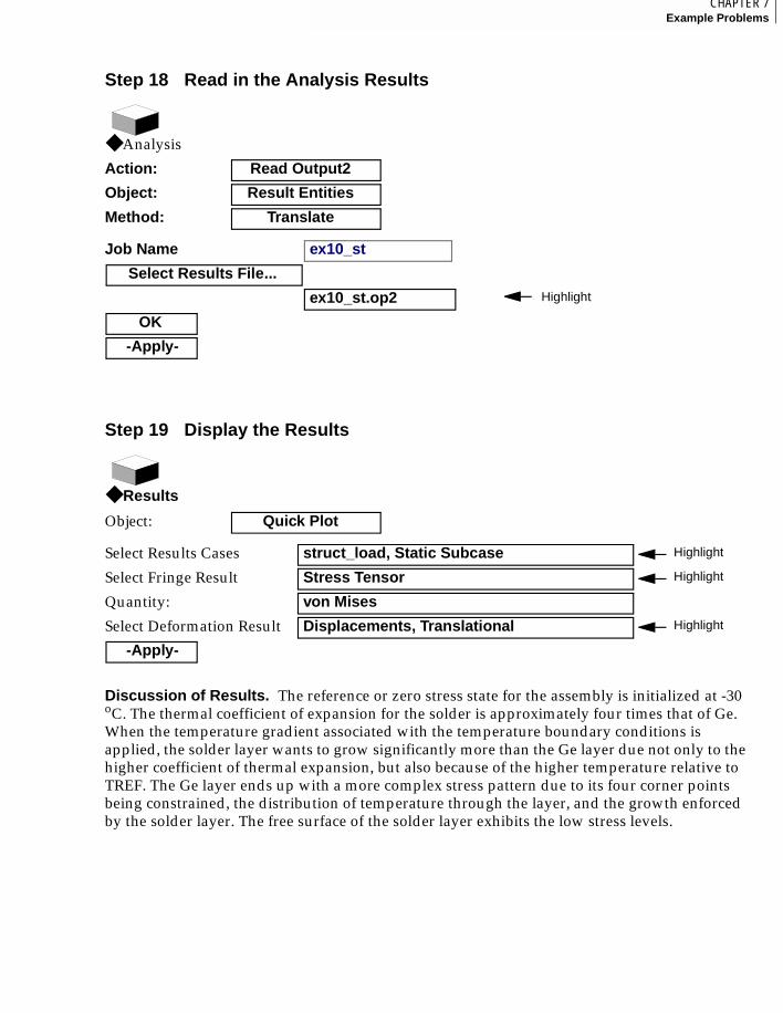
265CHAPTER 7Example Problems
7
Discussion of Results. The reference or zero stress state for the assembly is initialized at -30 oC. The thermal coefficient of expansion for the solder is approximately four times that of Ge. When the temperature gradient associated with the temperature boundary conditions is applied, the solder layer wants to grow significantly more than the Ge layer due not only to the higher coefficient of thermal expansion, but also because of the higher temperature relative to TREF. The Ge layer ends up with a more complex stress pattern due to its four corner points being constrained, the distribution of temperature through the layer, and the growth enforced by the solder layer. The free surface of the solder layer exhibits the low stress levels.
Step 18 Read in the Analysis Results
◆ Analysis
Action: Read Output2
Object: Result Entities
Method: Translate
Job Name ex10_st
Select Results File...
ex10_st.op2 Highlight
OK
-Apply-
Step 19 Display the Results
◆ Results
Object: Quick Plot
Select Results Cases struct_load, Static Subcase Highlight
Select Fringe Result Stress Tensor Highlight
Quantity: von Mises
Select Deformation Result Displacements, Translational Highlight
-Apply-

7
266

MSC.Patran MSC.Nastran Preference Guide, Volume 2: Thermal Analysis
APPENDIX
A Files
■ Files
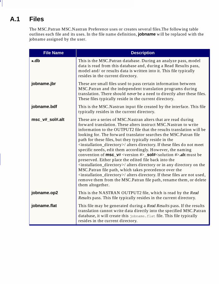
A
268
A.1 FilesThe MSC.Patran MSC.Nastran Preference uses or creates several files.The following table outlines each file and its uses. In the file name definition, jobname will be replaced with the jobname assigned by the user.
File Name Description
*.db This is the MSC.Patran database. During an analyze pass, model data is read from this database and, during a Read Results pass, model and/or results data is written into it. This file typically resides in the current directory.
jobname.jbr These are small files used to pass certain information between MSC.Patran and the independent translation programs during translation. There should never be a need to directly alter these files. These files typically reside in the current directory.
jobname.bdf This is the MSC.Nastran input file created by the interface. This file typically resides in the current directory.
msc_v#_sol#.alt These are a series of MSC.Nastran alters that are read during forward translation. These alters instruct MSC.Nastran to write information to the OUTPUT2 file that the results translation will be looking for. The forward translator searches the MSC.Patran file path for these files, but they typically reside in the <installation_directory>/alters directory. If these files do not meet specific needs, edit them accordingly. However, the naming convention of msc_v# <version #>_sol#<solution #>.alt must be preserved. Either place the edited file back into the <installation_directory>/alters directory or in any directory on the MSC.Patran file path, which takes precedence over the <installation_directory>/alters directory. If these files are not used, remove them from the MSC.Patran file path, rename them, or delete them altogether.
jobname.op2 This is the NASTRAN OUTPUT2 file, which is read by the Read Results pass. This file typically resides in the current directory.
jobname.flat This file may be generated during a Read Results pass. If the results translation cannot write data directly into the specified MSC.Patran database, it will create this jobname.flat file. This file typically resides in the current directory.
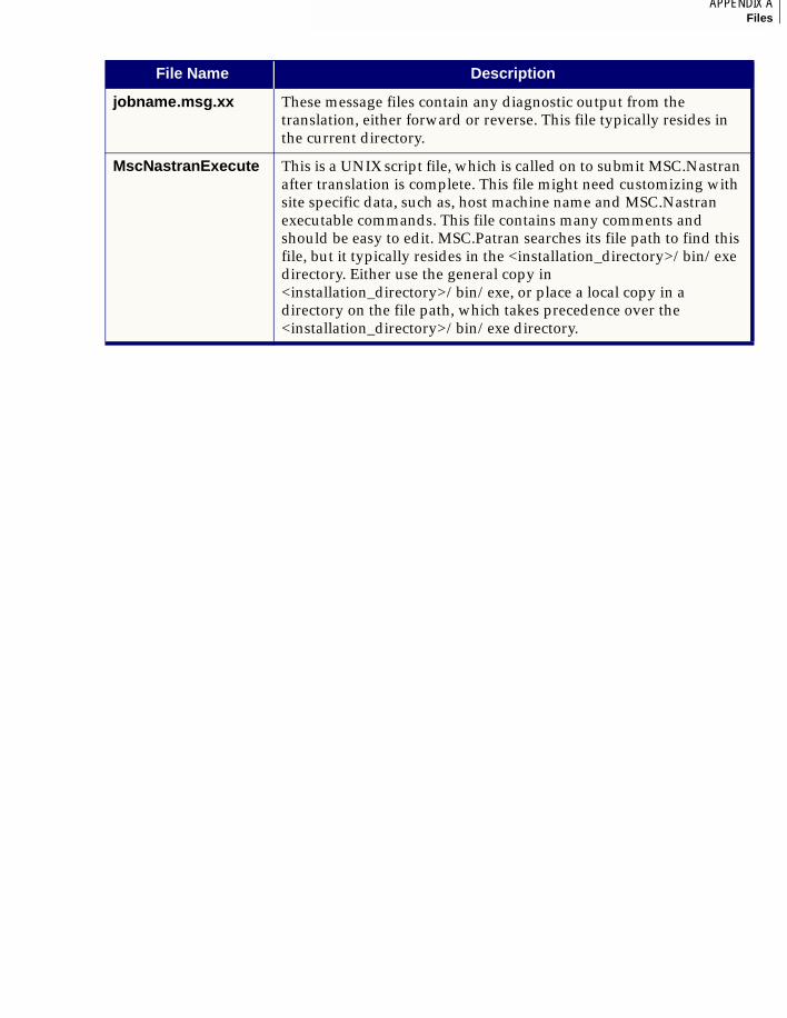
269APPENDIX AFiles
A
jobname.msg.xx These message files contain any diagnostic output from the translation, either forward or reverse. This file typically resides in the current directory.
MscNastranExecute This is a UNIX script file, which is called on to submit MSC.Nastran after translation is complete. This file might need customizing with site specific data, such as, host machine name and MSC.Nastran executable commands. This file contains many comments and should be easy to edit. MSC.Patran searches its file path to find this file, but it typically resides in the <installation_directory>/bin/exe directory. Either use the general copy in <installation_directory>/bin/exe, or place a local copy in a directory on the file path, which takes precedence over the <installation_directory>/bin/exe directory.
File Name Description

A
270

MSC.Patran MSC.Nastran Preference Guide, Volume 2: Thermal Analysis
APENDIX
B Error Messages
■ Error Messages
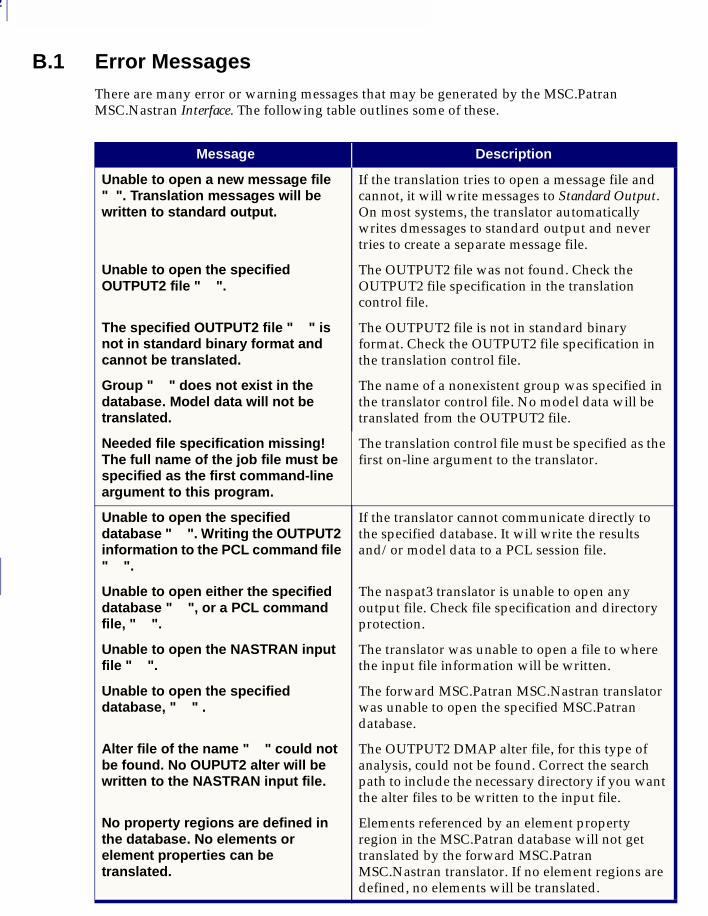
B
272
B.1 Error MessagesThere are many error or warning messages that may be generated by the MSC.Patran MSC.Nastran Interface. The following table outlines some of these.
Message Description
Unable to open a new message file " ". Translation messages will be written to standard output.
If the translation tries to open a message file and cannot, it will write messages to Standard Output. On most systems, the translator automatically writes dmessages to standard output and never tries to create a separate message file.
Unable to open the specified OUTPUT2 file " ".
The OUTPUT2 file was not found. Check the OUTPUT2 file specification in the translation control file.
The specified OUTPUT2 file " " is not in standard binary format and cannot be translated.
The OUTPUT2 file is not in standard binary format. Check the OUTPUT2 file specification in the translation control file.
Group " " does not exist in the database. Model data will not be translated.
The name of a nonexistent group was specified in the translator control file. No model data will be translated from the OUTPUT2 file.
Needed file specification missing! The full name of the job file must be specified as the first command-line argument to this program.
The translation control file must be specified as the first on-line argument to the translator.
Unable to open the specified database " ". Writing the OUTPUT2 information to the PCL command file " ".
If the translator cannot communicate directly to the specified database. It will write the results and/or model data to a PCL session file.
Unable to open either the specified database " ", or a PCL command file, " ".
The naspat3 translator is unable to open any output file. Check file specification and directory protection.
Unable to open the NASTRAN input file " ".
The translator was unable to open a file to where the input file information will be written.
Unable to open the specified database, " " .
The forward MSC.Patran MSC.Nastran translator was unable to open the specified MSC.Patran database.
Alter file of the name " " could not be found. No OUPUT2 alter will be written to the NASTRAN input file.
The OUTPUT2 DMAP alter file, for this type of analysis, could not be found. Correct the search path to include the necessary directory if you want the alter files to be written to the input file.
No property regions are defined in the database. No elements or element properties can be translated.
Elements referenced by an element property region in the MSC.Patran database will not get translated by the forward MSC.Patran MSC.Nastran translator. If no element regions are defined, no elements will be translated.

MSC.Patran MSC.Nastran Preference Guide, Volume 2: Thermal Analysis
APPENDIX
C Supported Commands
■ File Management Statements
■ Executive Control Statements
■ Case Control Commands
■ Bulk Data Entries

C
274
C.1 File Management StatementsThe following MSC.Nastran File Management statement is supported.
Command Description
ASSIGN An ASSIGN command is used to assign a particular name (job name + user specified MSC.Nastran results suffix) to the NASTRAN OUTPUT2 file to be created during the analysis.

275APPENDIX CSupported Commands
C
C.2 Executive Control StatementsThe following MSC.Nastran Executive Control statements are supported.
Command Description
SOL Specifies the solution sequence or main subDMAP to be executed. (p. 104)
TIME Sets the maximum CPU and I/O time.(p. 105), (p. 109)
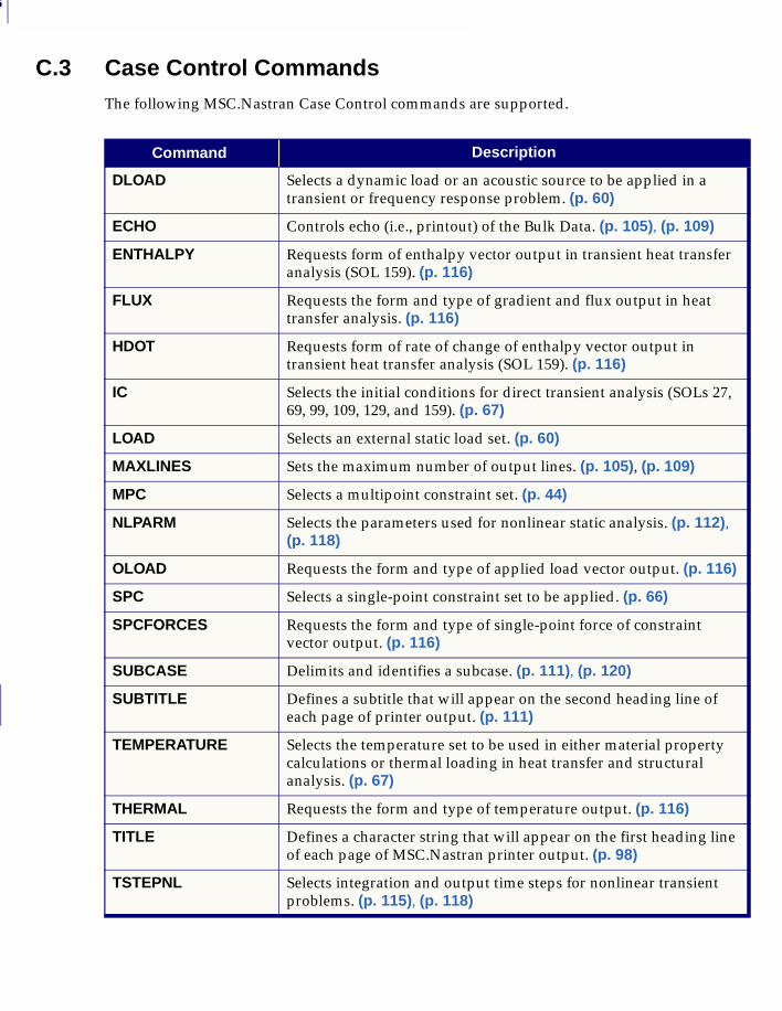
C
276
C.3 Case Control CommandsThe following MSC.Nastran Case Control commands are supported.
Command Description
DLOAD Selects a dynamic load or an acoustic source to be applied in a transient or frequency response problem. (p. 60)
ECHO Controls echo (i.e., printout) of the Bulk Data. (p. 105), (p. 109)
ENTHALPY Requests form of enthalpy vector output in transient heat transfer analysis (SOL 159). (p. 116)
FLUX Requests the form and type of gradient and flux output in heat transfer analysis. (p. 116)
HDOT Requests form of rate of change of enthalpy vector output in transient heat transfer analysis (SOL 159). (p. 116)
IC Selects the initial conditions for direct transient analysis (SOLs 27, 69, 99, 109, 129, and 159). (p. 67)
LOAD Selects an external static load set. (p. 60)
MAXLINES Sets the maximum number of output lines. (p. 105), (p. 109)
MPC Selects a multipoint constraint set. (p. 44)
NLPARM Selects the parameters used for nonlinear static analysis. (p. 112), (p. 118)
OLOAD Requests the form and type of applied load vector output. (p. 116)
SPC Selects a single-point constraint set to be applied. (p. 66)
SPCFORCES Requests the form and type of single-point force of constraint vector output. (p. 116)
SUBCASE Delimits and identifies a subcase. (p. 111), (p. 120)
SUBTITLE Defines a subtitle that will appear on the second heading line of each page of printer output. (p. 111)
TEMPERATURE Selects the temperature set to be used in either material property calculations or thermal loading in heat transfer and structural analysis. (p. 67)
THERMAL Requests the form and type of temperature output. (p. 116)
TITLE Defines a character string that will appear on the first heading line of each page of MSC.Nastran printer output. (p. 98)
TSTEPNL Selects integration and output time steps for nonlinear transient problems. (p. 115), (p. 118)
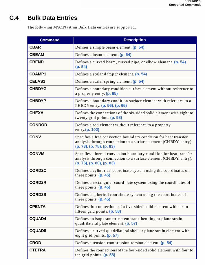
277APPENDIX CSupported Commands
C
C.4 Bulk Data EntriesThe following MSC.Nastran Bulk Data entries are supported.
Command Description
CBAR Defines a simple beam element. (p. 54)
CBEAM Defines a beam element. (p. 54)
CBEND Defines a curved beam, curved pipe, or elbow element. (p. 54) (p. 54)
CDAMP1 Defines a scalar damper element. (p. 54)
CELAS1 Defines a scalar spring element. (p. 54)
CHBDYG Defines a boundary condition surface element without reference to a property entry. (p. 65)
CHBDYP Defines a boundary condition surface element with reference to a PHBDY entry. (p. 56), (p. 65)
CHEXA Defines the connections of the six-sided solid element with eight to twenty grid points. (p. 58)
CONROD Defines a rod element without reference to a property entry.(p. 102)
CONV Specifies a free convection boundary condition for heat transfer analysis through connection to a surface element (CHBDYi entry). (p. 73), (p. 78), (p. 83)
CONVM Specifies a forced convection boundary condition for heat transfer analysis through connection to a surface element (CHBDYi entry). (p. 75), (p. 80), (p. 83)
CORD2C Defines a cylindrical coordinate system using the coordinates of three points. (p. 45)
CORD2R Defines a rectangular coordinate system using the coordinates of three points. (p. 45)
CORD2S Defines a spherical coordinate system using the coordinates of three points. (p. 45)
CPENTA Defines the connections of a five-sided solid element with six to fifteen grid points. (p. 58)
CQUAD4 Defines an isoparametric membrane-bending or plane strain quadrilateral plate element. (p. 57)
CQUAD8 Defines a curved quadrilateral shell or plane strain element with eight grid points. (p. 57)
CROD Defines a tension-compression-torsion element. (p. 54)
CTETRA Defines the connections of the four-sided solid element with four to ten grid points. (p. 58)
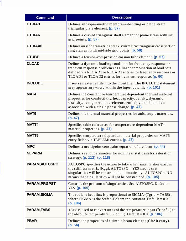
C
278
CTRIA3 Defines an isoparametric membrane-bending or plane strain triangular plate element. (p. 57)
CTRIA6 Defines a curved triangular shell element or plane strain with six grid points. (p. 57)
CTRIAX6 Defines an isoparametric and axisymmetric triangular cross section ring element with midside grid points. (p. 58)
CTUBE Defines a tension-compression-torsion tube element. (p. 57)
DLOAD Defines a dynamic loading condition for frequency response or transient response problems as a linear combination of load sets defined via RLOAD1 or RLOAD2 entries for frequency response or TLOAD1 or TLOAD2 entries for transient response. (p. 60)
INCLUDE Inserts an external file into the input file. The INCLUDE statement may appear anywhere within the input data file. (p. 101)
MAT4 Defines the constant or temperature dependent thermal material properties for conductivity, heat capacity, density, dynamic viscosity, heat generation, reference enthalpy and latent heat associated with a single phase change. (p. 47)
MAT5 Defines the thermal material properties for anisotropic materials. (p. 47)
MATT4 Specifies table references for temperature-dependent MAT4 material properties. (p. 47)
MATT5 Specifies temperature-dependent material properties on MAT5 entry fields via TABLEMi entries. (p. 47)
MPC Defines a multipoint constraint equation of the form. (p. 44)
NLPARM Defines a set of parameters for nonlinear static analysis iteration strategy. (p. 112), (p. 118)
PARAM,AUTOSPC AUTOSPC specifies the action to take when singularities exist in the stiffness matrix [Kgg]. AUTOSPC = YES means that singularities will be constrained automatically. AUTOSPC = NO means that singularities will not be constrained. (p. 105)
PARAM,PRGPST Controls the printout of singularities. See AUTOSPC. Default = YES. (p. 109)
PARAM,SIGMA The radiant heat flux is proportional to SIGMA*(Tgrid + TABS)4, where SIGMA is the Stefan-Boltzmann constant. Default = 0.0. (p. 106)
PARAM,TABS TABS is used to convert units of the temperature input (oF or oC) to the absolute temperature (°R or °K). Default = 0.0. (p. 106)
PBAR Defines the properties of a simple beam element (CBAR entry). (p. 54)
Command Description
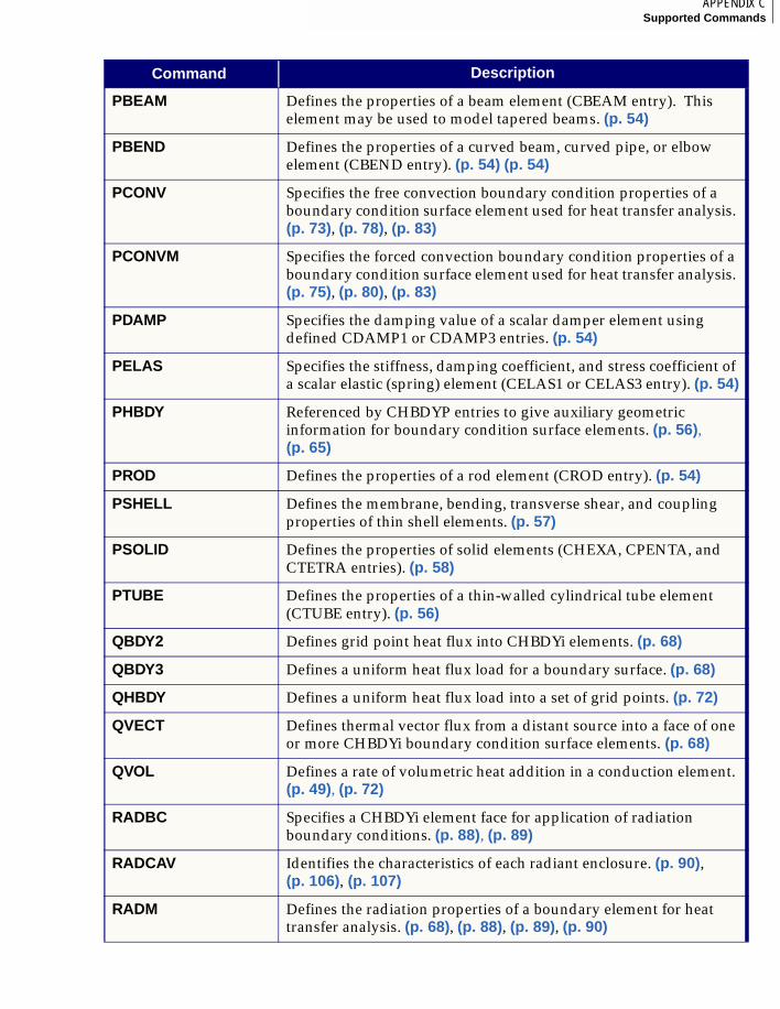
279APPENDIX CSupported Commands
C
PBEAM Defines the properties of a beam element (CBEAM entry). This element may be used to model tapered beams. (p. 54)
PBEND Defines the properties of a curved beam, curved pipe, or elbow element (CBEND entry). (p. 54) (p. 54)
PCONV Specifies the free convection boundary condition properties of a boundary condition surface element used for heat transfer analysis. (p. 73), (p. 78), (p. 83)
PCONVM Specifies the forced convection boundary condition properties of a boundary condition surface element used for heat transfer analysis. (p. 75), (p. 80), (p. 83)
PDAMP Specifies the damping value of a scalar damper element using defined CDAMP1 or CDAMP3 entries. (p. 54)
PELAS Specifies the stiffness, damping coefficient, and stress coefficient of a scalar elastic (spring) element (CELAS1 or CELAS3 entry). (p. 54)
PHBDY Referenced by CHBDYP entries to give auxiliary geometric information for boundary condition surface elements. (p. 56), (p. 65)
PROD Defines the properties of a rod element (CROD entry). (p. 54)
PSHELL Defines the membrane, bending, transverse shear, and coupling properties of thin shell elements. (p. 57)
PSOLID Defines the properties of solid elements (CHEXA, CPENTA, and CTETRA entries). (p. 58)
PTUBE Defines the properties of a thin-walled cylindrical tube element (CTUBE entry). (p. 56)
QBDY2 Defines grid point heat flux into CHBDYi elements. (p. 68)
QBDY3 Defines a uniform heat flux load for a boundary surface. (p. 68)
QHBDY Defines a uniform heat flux load into a set of grid points. (p. 72)
QVECT Defines thermal vector flux from a distant source into a face of one or more CHBDYi boundary condition surface elements. (p. 68)
QVOL Defines a rate of volumetric heat addition in a conduction element. (p. 49), (p. 72)
RADBC Specifies a CHBDYi element face for application of radiation boundary conditions. (p. 88), (p. 89)
RADCAV Identifies the characteristics of each radiant enclosure. (p. 90), (p. 106), (p. 107)
RADM Defines the radiation properties of a boundary element for heat transfer analysis. (p. 68), (p. 88), (p. 89), (p. 90)
Command Description
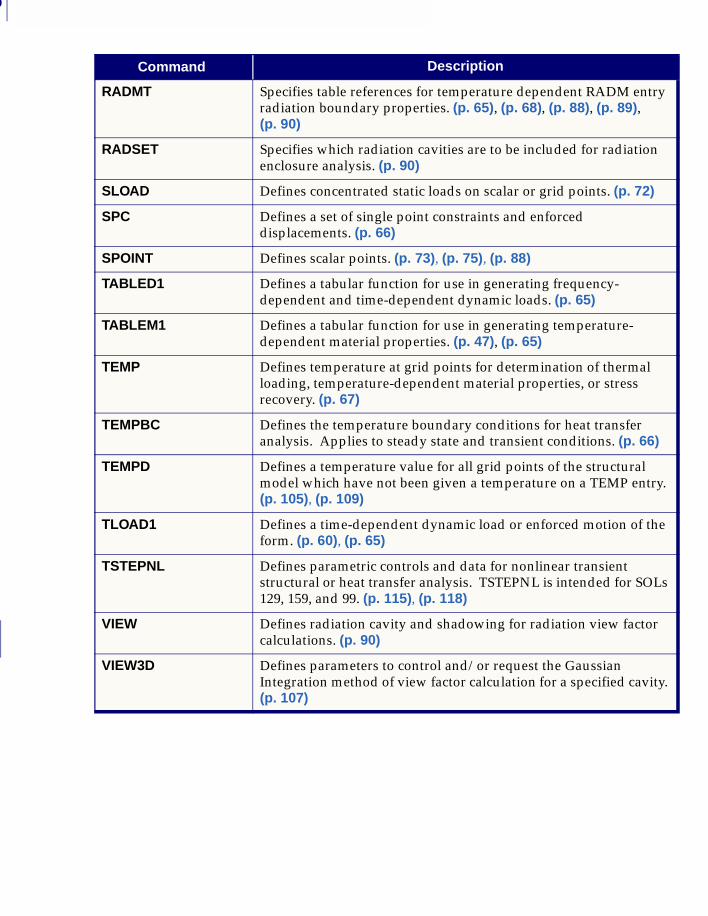
C
280
RADMT Specifies table references for temperature dependent RADM entry radiation boundary properties. (p. 65), (p. 68), (p. 88), (p. 89), (p. 90)
RADSET Specifies which radiation cavities are to be included for radiation enclosure analysis. (p. 90)
SLOAD Defines concentrated static loads on scalar or grid points. (p. 72)
SPC Defines a set of single point constraints and enforced displacements. (p. 66)
SPOINT Defines scalar points. (p. 73), (p. 75), (p. 88)
TABLED1 Defines a tabular function for use in generating frequency-dependent and time-dependent dynamic loads. (p. 65)
TABLEM1 Defines a tabular function for use in generating temperature-dependent material properties. (p. 47), (p. 65)
TEMP Defines temperature at grid points for determination of thermal loading, temperature-dependent material properties, or stress recovery. (p. 67)
TEMPBC Defines the temperature boundary conditions for heat transfer analysis. Applies to steady state and transient conditions. (p. 66)
TEMPD Defines a temperature value for all grid points of the structural model which have not been given a temperature on a TEMP entry. (p. 105), (p. 109)
TLOAD1 Defines a time-dependent dynamic load or enforced motion of the form. (p. 60), (p. 65)
TSTEPNL Defines parametric controls and data for nonlinear transient structural or heat transfer analysis. TSTEPNL is intended for SOLs 129, 159, and 99. (p. 115), (p. 118)
VIEW Defines radiation cavity and shadowing for radiation view factor calculations. (p. 90)
VIEW3D Defines parameters to control and/or request the Gaussian Integration method of view factor calculation for a specified cavity. (p. 107)
Command Description
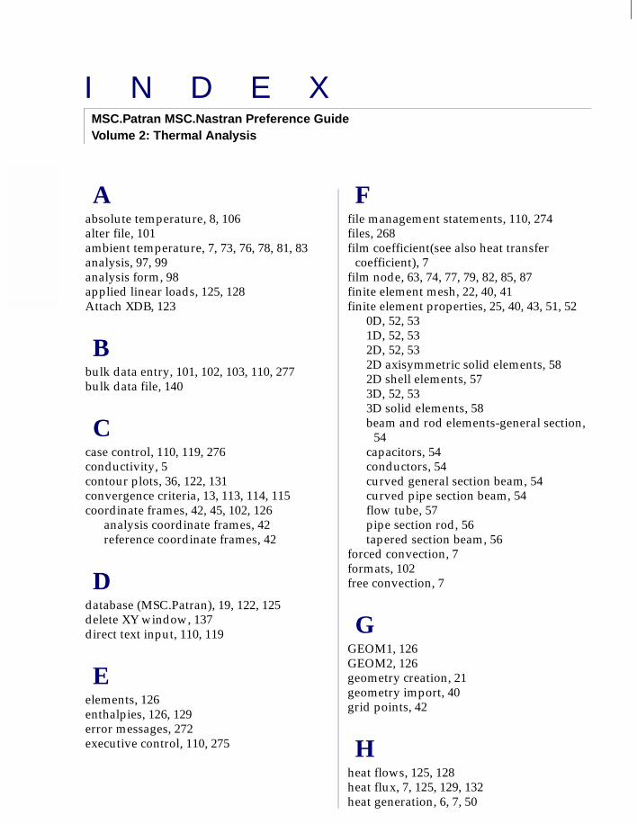
Index
281
I N D E XMSC.Patran MSC.Nastran Preference Guide Volume 2: Thermal Analysis
I N D E XMSC.Patran MSC.Nastran
Preference Guide
Volume 2: Thermal
Analysis
Aabsolute temperature, 8, 106alter file, 101ambient temperature, 7, 73, 76, 78, 81, 83analysis, 97, 99analysis form, 98applied linear loads, 125, 128Attach XDB, 123
Bbulk data entry, 101, 102, 103, 110, 277bulk data file, 140
Ccase control, 110, 119, 276conductivity, 5contour plots, 36, 122, 131convergence criteria, 13, 113, 114, 115coordinate frames, 42, 45, 102, 126
analysis coordinate frames, 42reference coordinate frames, 42
Ddatabase (MSC.Patran), 19, 122, 125delete XY window, 137direct text input, 110, 119
Eelements, 126enthalpies, 126, 129error messages, 272executive control, 110, 275
Ffile management statements, 110, 274files, 268film coefficient(see also heat transfer
coefficient), 7film node, 63, 74, 77, 79, 82, 85, 87finite element mesh, 22, 40, 41finite element properties, 25, 40, 43, 51, 52
0D, 52, 531D, 52, 532D, 52, 532D axisymmetric solid elements, 582D shell elements, 573D, 52, 533D solid elements, 58beam and rod elements-general section,
54capacitors, 54conductors, 54curved general section beam, 54curved pipe section beam, 54flow tube, 57pipe section rod, 56tapered section beam, 56
forced convection, 7formats, 102free convection, 7
GGEOM1, 126GEOM2, 126geometry creation, 21geometry import, 40grid points, 42
Hheat flows, 125, 128heat flux, 7, 125, 129, 132heat generation, 6, 7, 50
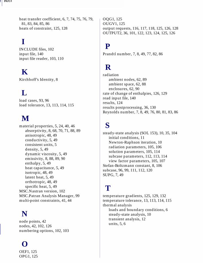
Index
INDEX282
heat transfer coefficient, 6, 7, 74, 75, 76, 79, 81, 83, 84, 85, 86
heats of constraint, 125, 128
IINCLUDE files, 102input file, 140input file reader, 103, 110
KKirchhoff’s Identity, 8
Lload cases, 93, 96load tolerance, 13, 113, 114, 115
Mmaterial properties, 5, 24, 40, 46
absorptivity, 8, 68, 70, 71, 88, 89anisotropic, 48, 49conductivity, 5, 49consistent units, 5density, 5, 49dynamic viscosity, 5, 49emissivity, 8, 88, 89, 90enthalpy, 5, 49heat capacitance, 5, 49isotropic, 48, 49latent heat, 5, 49orthotropic, 48, 49specific heat, 5, 49
MSC.Nastran version, 102MSC.Patran Analysis Manager, 99multi-point constraints, 41, 44
Nnode points, 42nodes, 42, 102, 126numbering options, 102, 103
OOEF1, 125OPG1, 125
OQG1, 125OUGV1, 125output requests, 116, 117, 118, 125, 126, 128OUTPUT2, 36, 101, 122, 123, 124, 125, 126
PPrandtl number, 7, 8, 49, 77, 82, 86
Rradiation
ambient nodes, 62, 89ambient space, 62, 88enclosures, 62, 90
rate of change of enthalpies, 126, 129read input file, 140results, 124results postprocessing, 36, 130Reynolds number, 7, 8, 49, 76, 80, 81, 83, 86
Ssteady-state analysis (SOL 153), 10, 35, 104
initial conditions, 11Newton-Raphson iteration, 10radiation parameters, 105, 106solution parameters, 105, 114subcase parameters, 112, 113, 114view factor parameters, 105, 107
Stefan-Boltzmann constant, 8, 106subcase, 96, 99, 111, 112, 120SUPG, 7, 49
Ttemperature gradients, 125, 129, 132temperature tolerance, 13, 113, 114, 115thermal analysis
loads and boundary conditions, 6steady-state analysis, 10transient analysis, 12units, 5, 6
Index
283INDEX
thermal loads and BCs, 6, 40, 59, 60advection, forced convection, 7, 61basic convection, 7, 32, 61consistent units, 6control nodes, 63, 68, 71, 72convection coupled, 78convection coupled advection, 83convection coupled flow tube, 80convection flow tube to ambient, 75convection to ambient, 73directional heat flux, 6, 61, 68, 71directional heat flux-function of time, 71flow tubes, 75, 80, 83initial temperatures, 67nodal source, 7, 61, 72normal heat flux, 6, 29, 61, 68radiation enclosures, 8, 62, 90radiation to ambient nodes, 89radiation to space, 8, 62, 88spatial dependence, 65surface area, 65temperature boundary conditions, 6, 27,
61, 66temperature dependence, 65time dependence, 65two application regions, 64, 78, 80, 83, 89volumetric heat generation, 7, 48, 50, 61,
72tolerances, 101transient analysis (SOL 159), 12, 104
initial conditions, 13initial time step, 12, 115solution parameters, 109subcase parameters, 115
translation parameters, 101, 102
Uundo feature, 23
Vview factors, 8, 88, 107, 108
Wwork tolerance, 13, 113, 114, 115
XXY plots, 122, 133, 135

Index
INDEX284


![[ From the Beginning ] - MSC Software...MSC.Nastran, MSC.Patran and MSC.ADAMS from MSC's portfolio of best-in-class technologies. Under BTCC rules only certain modifications to the](https://img.pdfslide.us/doc/110x75/5e8bf529fc07524daa691095/-from-the-beginning-msc-software-mscnastran-mscpatran-and-mscadams.jpg)