Embed Size (px)
Citation preview
C O N T E N T SMSC.Patran Thermal User’s Guide Volume 2: Viewfactor Analysis MSC.Patran Thermal User’s Guide,
Volume 2:
CHAPTER
1Introduction ■ About the Viewfactor Program, 2
■ Features and Benefits, 3
■ About this Guide, 5
■ Using this Guide, 6❑ Assumptions About the User, 6❑ Other Pertinent Documents, 6
■ Guide Organization, 7
■ Overview of Viewfactor Analysis, 8
■ Nomenclature, 10❑ Conventions, 10❑ Units, 10
2Overview ■ Purpose, 12
■ Relationship of Viewfactor to MSC.Patran and MSC.Patran Thermal, 13❑ Description, 14
■ Viewfactor Data and Program Flow, 16❑ Description, 16
■ Summary of the Analysis Cycle for a Thermal Radiation Problem, 20❑ Problem Definition, 20❑ General Preprocessing, 20❑ General MSC.Patran Thermal Preparation, 20❑ Thermal Radiation Specific Preprocessing, 21❑ Preparation for Viewfactor Analysis, 21❑ Viewfactor Analysis, 22❑ Post Viewfactor Analysis, 22❑ MSC.Patran Thermal Analysis, 22❑ Postprocessing, 23❑ Refinements, 23
3Model Creation for a Thermal Radiation Problem
■ Purpose, 26
■ Radiation Enclosure Concept, 27❑ Definition of Enclosure, 27
❑ The Enclosure ID, 27❑ Wavebands and Enclosures, 28❑ Examples of the Use of Enclosures, 29
■ Surface Orientation in MSC.Patran, 35❑ The Importance of Surface Orientation, 35❑ Determining Surface Orientation, 39❑ Correcting Improper Surface Orientations, 41❑ Suggested Practices for Creating Properly Oriented Surfaces, 42
■ Specifying Radiation Boundary Conditions Using MSC.Patran Reference Manual (VFAC Boundary Condition), 43
❑ Purpose of the Viewfactor Form, 43❑ Form for the VFAC LBC, 44❑ Requirement for Oriented 2-D Surfaces Related to the VFAC LBC, 47❑ Neutral File Data Packet Created from the VFAC LBC, 47
■ Advanced Features of the VFAC Boundary Condition, 48❑ Referencing Participating Media Radiation Nodes, 48❑ Referencing Ambient or Space Radiation Nodes, 51❑ Identifying a Surface as Being Convex, 55❑ Identifying a Surface as Not Obstructing the View Between Other Surface
Pairs, 57
■ Relationship of VFAC LBC Data to VFINDAT File Data, 59
■ MSC.Patran Thermal TEMPLATEDAT Files for Surface Property Description, 60
❑ Thermal Radiation Wavebands as Used in MSC.Patran Thermal User’s Guide, 60
❑ Radiation Resistor Types Used in MSC.Patran Thermal, 62❑ MSC.Patran Thermal MPIDs (Material Property IDs), 65❑ MSC.Patran Thermal Material Property Definition, 67❑ VFAC Template Format, 68❑ Examples of TEMPLATEDAT Files for Thermal Radiation, 72
■ Compatibility Requirements for Model and VFAC Templates, 75❑ Origin of the Problem, 75❑ Suggested Procedures to Avoid Compatibility Problems, 76
■ Symmetry as Applied to the Model and Viewfactor Radiation Exchange, 77❑ The Purpose of Symmetry in Viewfactor, 77❑ Caveats Concerning the Use of Symmetry in Thermal Radiation
Modeling, 77❑ Symmetry Operations Supported in Viewfactor, 78❑ Example of the Use of Symmetry in Thermal Radiation Modeling, 84❑ Example Which Appears Symmetric, But in Fact Is Not Symmetric, 85❑ Entering Viewfactor Symmetry Operations in the MSC.Patran Model, 86
4Preparation for Analysis
■ Introduction, 88
■ Viewfactor Execution From MSC.Patran Thermal, 89
■ PATQ Translation from the MSC.Patran Neutral File to the VFINDAT File, 90❑ Spawning From MSC.Patran vs. Stand-Alone Execution, 90
❑ Step-by-Step Procedure (Stand-Alone Execution), 91
■ VFCTL, the Viewfactor Program Execution Control File, 95❑ Philosophy and Structure of the VFCTL File, 95❑ Keywords in the VFCTL File, 98
5Analysis ■ Submitting a Viewfactor Job for Analysis, 108
❑ Review the Viewfactor Control/Parameters, 108❑ Review Directory for Required Files, 109❑ The Viewfactor Command Line, 110
■ Output Created by a Viewfactor Execution, 111❑ VFMSG, 111❑ VFDIAG, 112❑ VFRAWDAT, 113❑ VFRESDAT, 113❑ VFNODEDAT, 113
■ Reviewing the Viewfactor Output, 114❑ VFMSG, the Viewfactor Message File, 114❑ VFDIAG, the Viewfactor Diagnostic Data File, 118
6Post-Analysis ■ Introduction, 122
■ Interface From Viewfactor to MSC.Patran Thermal, 123❑ Viewfactor VFRESDAT and VFNODEDAT Files as Input to MSC.Patran
Thermal’s QTRAN, 123❑ Translating Binary Resistor File VFRESDAT to a Text File, VFRESTXT, 124
■ Notes on Resistor Values, 126
■ THERMAL Analysis, 127
■ THERMAL Results Postprocessing, 128
7Changing the Surface Template Data After Viewfactors are Calculated
■ Introduction, 130
■ Compatible VFAC LBC and Template Data, 131
■ New Resistors from Raw Viewfactor Data, 132❑ Changing TEMPLATEDAT VFAC Templates, 132❑ Changing MSC.Patran Thermal Material Definitions, 132❑ Changing VFCTL, 132❑ Submitting the New Viewfactor Job, 132
8Theory and Computational Limitations
■ Introduction, 134
■ Viewfactor, 135
■ Mean Beam Length, 136
■ Obstructions, 138
■ Computational Limitations, 139❑ Grazing Incidence of the Intersurface Ray with the Surface, 139❑ Spatial Resolution, 139❑ Extreme Scales, 140
9Data File Specifications
■ Introduction, 142
■ VFINDAT (Input Data File), 143❑ Examples, 144❑ Detailed Descriptions, 146
■ VFRAWDAT (Raw Viewfactor Data), 150
■ VFRESDAT (Resistor Data), 154
■ VFDIAG (Diagnostic Data), 155❑ Introduction, 155❑ Examples, 156❑ Detailed Descriptions, 158
■ TEMPLATEDAT (Surface Pointer Data), 160
■ VFNODEDAT (Radiosity Node Lists), 162
10Rules for Radiation Resistors
■ Introduction, 164
■ General Rules for Radiation Resistors, 165
■ Rules for Emissivity Resistors, 166
■ Rules for Radiosity Resistors, 167
ATypical Errors and Probable Causes for Viewfactor Errors
■ Purpose, 170
BQuick Reference Guide to Viewfactor
■ Purpose, 172
CMemory Requirements for Viewfactor Execution
■ Purpose, 176
DMachine-Specific File Names for Viewfactor
■ Purpose, 178
EExample Thermal Radiation Problems
■ Purpose, 180
■ Problem 1 - Steady-State Radiative Boundary Conditions, 181❑ Objectives, 181❑ Model Description, 181❑ Exercise Procedure, 182
■ Problem 2 - Parallel Semi-Infinite Plates, 200
■ Problem 3 - Heated Reaction Chamber, 204
INDEX ■ MSC.Patran Thermal User’s Guide, 209Volume 2: Viewfactor Analysis


MSC.Patran Thermal User’s Guide, Volume 2: Viewfactor Analysis
CHAPTER
1 Introduction
■ About the Viewfactor Program
■ Features and Benefits
■ About this Guide
■ Using this Guide
■ Guide Organization
■ Overview of Viewfactor Analysis
■ Nomenclature

Volume 2Viewfactor Analysis
1.1 About the Viewfactor ProgramThe Viewfactor program in the MSC.Patran system is designed to facilitate the generation of finite element based radiation viewfactors. These viewfactor calculations are intended to be used as input into the MSC.Patran Thermal analysis code, although there should be nothing to stop it from being used in conjunction with other similar thermal analysis codes. It was primarily designed to fill a void in the thermal capabilities of the MSC.Patran system and to further expand the potential application of the MSC.Patran Thermal module.
3CHAPTER 1Introduction
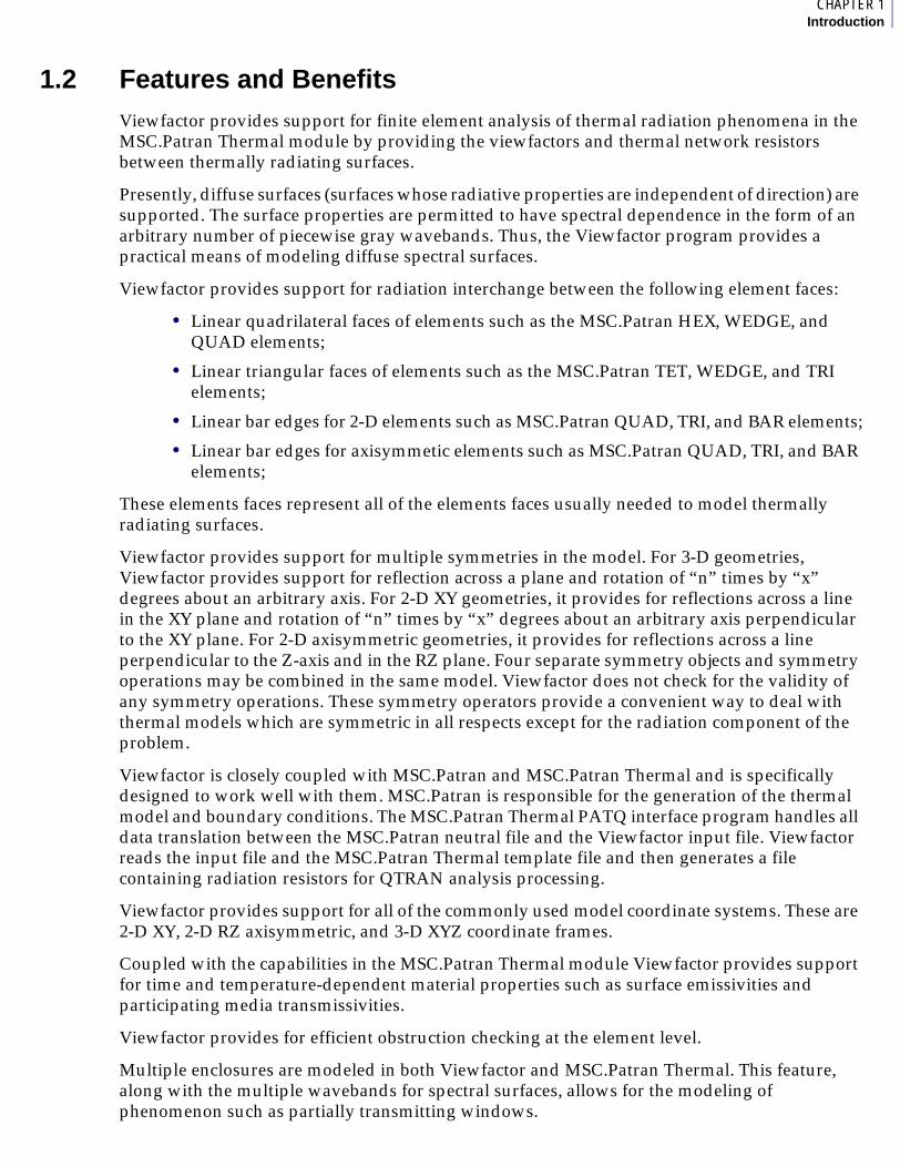
1.2 Features and BenefitsViewfactor provides support for finite element analysis of thermal radiation phenomena in the MSC.Patran Thermal module by providing the viewfactors and thermal network resistors between thermally radiating surfaces.
Presently, diffuse surfaces (surfaces whose radiative properties are independent of direction) are supported. The surface properties are permitted to have spectral dependence in the form of an arbitrary number of piecewise gray wavebands. Thus, the Viewfactor program provides a practical means of modeling diffuse spectral surfaces.
Viewfactor provides support for radiation interchange between the following element faces:
• Linear quadrilateral faces of elements such as the MSC.Patran HEX, WEDGE, and QUAD elements;
• Linear triangular faces of elements such as the MSC.Patran TET, WEDGE, and TRI elements;
• Linear bar edges for 2-D elements such as MSC.Patran QUAD, TRI, and BAR elements;
• Linear bar edges for axisymmetic elements such as MSC.Patran QUAD, TRI, and BAR elements;
These elements faces represent all of the elements faces usually needed to model thermally radiating surfaces.
Viewfactor provides support for multiple symmetries in the model. For 3-D geometries, Viewfactor provides support for reflection across a plane and rotation of “n” times by “x” degrees about an arbitrary axis. For 2-D XY geometries, it provides for reflections across a line in the XY plane and rotation of “n” times by “x” degrees about an arbitrary axis perpendicular to the XY plane. For 2-D axisymmetric geometries, it provides for reflections across a line perpendicular to the Z-axis and in the RZ plane. Four separate symmetry objects and symmetry operations may be combined in the same model. Viewfactor does not check for the validity of any symmetry operations. These symmetry operators provide a convenient way to deal with thermal models which are symmetric in all respects except for the radiation component of the problem.
Viewfactor is closely coupled with MSC.Patran and MSC.Patran Thermal and is specifically designed to work well with them. MSC.Patran is responsible for the generation of the thermal model and boundary conditions. The MSC.Patran Thermal PATQ interface program handles all data translation between the MSC.Patran neutral file and the Viewfactor input file. Viewfactor reads the input file and the MSC.Patran Thermal template file and then generates a file containing radiation resistors for QTRAN analysis processing.
Viewfactor provides support for all of the commonly used model coordinate systems. These are 2-D XY, 2-D RZ axisymmetric, and 3-D XYZ coordinate frames.
Coupled with the capabilities in the MSC.Patran Thermal module Viewfactor provides support for time and temperature-dependent material properties such as surface emissivities and participating media transmissivities.
Viewfactor provides for efficient obstruction checking at the element level.
Multiple enclosures are modeled in both Viewfactor and MSC.Patran Thermal. This feature, along with the multiple wavebands for spectral surfaces, allows for the modeling of phenomenon such as partially transmitting windows.

Volume 2Viewfactor Analysis
No fixed problem size limit exists for Viewfactor. Memory for the particular model being analyzed is allocated during run time. Problem size is limited only by available virtual memory, available CPU resources, and storage space for the output data. Core memory requirements are linear functions of the model size, not higher order functions as is true for some viewfactor analysis programs.
Through use of the MSC.Patran Thermal template file, Viewfactor provides support for optically thin participating media.
The geometric calculations involved in determining obstructions and viewfactors are saved as an intermediate result and can be reused with different material properties in the same model. These CPU intensive calculations need not be repeated when material properties change.
Viewfactor checks for convergence of its numerical integration algorithms and increases or decreases the integration order as appropriate. This provides excellent performance as measured by the product of accuracy and speed.
Diagnostic data is provided to aid in verifying the accuracy of an analysis.
Viewfactor provides support for radiation to an ambient or space environment node.
Convex surfaces may be flagged to help reduce execution time.
Nonobstructing surfaces may be flagged in order to reduce the time required to check for obstructed views.

5CHAPTER 1Introduction
1.3 About this GuideThis Guide contains a complete description of MSC.Patran Thermal’s Viewfactor code. The thermal phenomena that this module is designed to model are technically complex. Great care has been taken to present the material contained herein in a manner that is clear and easy to understand. Numerous examples throughout the text illustrate the subject matter.

Volume 2Viewfactor Analysis
1.4 Using this GuideThe material in this document is presented with certain assumptions about the knowledge and abilities of the user. It is recommended that the user obtain and become familiar with the other pertinent documents listed at the end of this section. This Guide makes frequent reference to these documents, or to material described more fully in them.
Assumptions About the UserThis document was written under the following assumptions:
• The user is familiar with MSC.Patran and can make finite element models in MSC.Patran. If not sufficiently versed in the use of MSC.Patran, the user may refer to the MSC.Patran Reference Manual or attend an MSC Institute course.
• The user is familiar with MSC.Software Corporation (MSC) product MSC.Patran Thermal and is able to perform thermal analysis using MSC.Patran and MSC.Patran Thermal. If not, the user may wish to refer to the MSC.Patran Thermal documentation and/or attend the MSC Institute course on MSC.Patran Thermal or obtain the video cassette course on MSC.Patran Thermal.
• The user is familiar with the computer environment in which this software will be used, and is able to manipulate files, manipulate directories, and edit files.
• The user has experience and/or education equivalent to a BS in engineering with an emphasis on thermal analysis. If the user is a novice thermal analyst, it is suggested that course work or self-directed study be undertaken. It is not the purpose of this Guide to make the user of Viewfactor a thermal analyst. The ideas presented and used in this Guide will not be easily understood by one who does not understand thermal analysis.
• Some of the material in this document is aimed at the thermal analysis expert.
Other Pertinent Documents• MSC.Patran Reference Manual, Volumes 1 through 3.
• MSC.Patran Thermal User’s Guide.
• Gebhart, B. Heat Transfer, 2nd edition, McGraw-Hill, 1971.
• Howell, J.R. A Catalog of Radiation Configuration Factors, McGraw-Hill, 1982.
• Siegel, R., and Howell, J.R. Thermal Radiation Heat Transfer, 2nd edition, McGraw-Hill, 1981.

7CHAPTER 1Introduction
1.5 Guide Organization The contents of this Guide are organized into four subject groupings. Each group is described in the following paragraphs, along with the chapters or appendices associated with each group. The four groups are:
❏ Introduction and Overview❏ The Analysis Cycle❏ Theory and Specifications❏ Examples
In addition, there are appendices at the end of the document which provide supplemental information on a number of topics. The Guide also has a comprehensive index to aid the reader in locating information on particular topics.
Volume 2Viewfactor Analysis
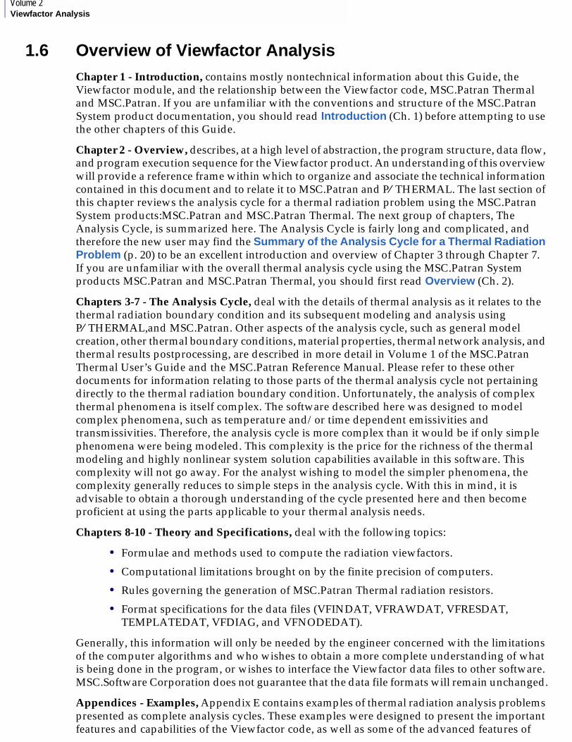
1.6 Overview of Viewfactor AnalysisChapter 1 - Introduction, contains mostly nontechnical information about this Guide, the Viewfactor module, and the relationship between the Viewfactor code, MSC.Patran Thermal and MSC.Patran. If you are unfamiliar with the conventions and structure of the MSC.Patran System product documentation, you should read Introduction (Ch. 1) before attempting to use the other chapters of this Guide.
Chapter 2 - Overview, describes, at a high level of abstraction, the program structure, data flow, and program execution sequence for the Viewfactor product. An understanding of this overview will provide a reference frame within which to organize and associate the technical information contained in this document and to relate it to MSC.Patran and P⁄ THERMAL. The last section of this chapter reviews the analysis cycle for a thermal radiation problem using the MSC.Patran System products:MSC.Patran and MSC.Patran Thermal. The next group of chapters, The Analysis Cycle, is summarized here. The Analysis Cycle is fairly long and complicated, and therefore the new user may find the Summary of the Analysis Cycle for a Thermal Radiation Problem (p. 20) to be an excellent introduction and overview of Chapter 3 through Chapter 7. If you are unfamiliar with the overall thermal analysis cycle using the MSC.Patran System products MSC.Patran and MSC.Patran Thermal, you should first read Overview (Ch. 2).
Chapters 3-7 - The Analysis Cycle, deal with the details of thermal analysis as it relates to the thermal radiation boundary condition and its subsequent modeling and analysis using P⁄ THERMAL,and MSC.Patran. Other aspects of the analysis cycle, such as general model creation, other thermal boundary conditions, material properties, thermal network analysis, and thermal results postprocessing, are described in more detail in Volume 1 of the MSC.Patran Thermal User’s Guide and the MSC.Patran Reference Manual. Please refer to these other documents for information relating to those parts of the thermal analysis cycle not pertaining directly to the thermal radiation boundary condition. Unfortunately, the analysis of complex thermal phenomena is itself complex. The software described here was designed to model complex phenomena, such as temperature and/or time dependent emissivities and transmissivities. Therefore, the analysis cycle is more complex than it would be if only simple phenomena were being modeled. This complexity is the price for the richness of the thermal modeling and highly nonlinear system solution capabilities available in this software. This complexity will not go away. For the analyst wishing to model the simpler phenomena, the complexity generally reduces to simple steps in the analysis cycle. With this in mind, it is advisable to obtain a thorough understanding of the cycle presented here and then become proficient at using the parts applicable to your thermal analysis needs.
Chapters 8-10 - Theory and Specifications, deal with the following topics:
• Formulae and methods used to compute the radiation viewfactors.
• Computational limitations brought on by the finite precision of computers.
• Rules governing the generation of MSC.Patran Thermal radiation resistors.
• Format specifications for the data files (VFINDAT, VFRAWDAT, VFRESDAT, TEMPLATEDAT, VFDIAG, and VFNODEDAT).
Generally, this information will only be needed by the engineer concerned with the limitations of the computer algorithms and who wishes to obtain a more complete understanding of what is being done in the program, or wishes to interface the Viewfactor data files to other software. MSC.Software Corporation does not guarantee that the data file formats will remain unchanged.
Appendices - Examples, Appendix E contains examples of thermal radiation analysis problems presented as complete analysis cycles. These examples were designed to present the important features and capabilities of the Viewfactor code, as well as some of the advanced features of

9CHAPTER 1Introduction
MSC.Patran Thermal as they pertain to analysis of thermal radiation problems. The problems are generally simple in other aspects and thus are easy to model and not too time-consuming. Once you have gained sufficient understanding of the analysis cycle, a quick review of the example problems will refresh your memory after you’ve been away from this software for a period of time. Some of the examples were also designed to demonstrate the correctness of the thermal analysis and to build confidence in the use of the Viewfactor code.
Other topics covered in the appendices are error conditions, memory requirements, and technical support.

Volume 2Viewfactor Analysis
1.7 NomenclatureCertain documentation conventions (such as different typefaces having meaning), special characters with specific meaning (such as slashes in MSC.Patran commands), technical definitions, and symbols used in this document are defined or described in this section.
Conventions
Font Types and Typefaces. Computer messages or responses are printed in plain character format:
SYSTEM RESPONSES ARE IN A PLAIN LETTER STYLE
Commands (or queries) that you enter are printed in bold typeface which is darker and heavier than normal or plain text:
commands entered by the user are in bold type
Some fields, or parts of a surface, may be optional. Fields contained within brackets [ ] are optional for data input. Generally, optional data fields that do not receive input will default to a predetermined value.
VFAC,TID[,NBANDS]
Filenames. A generic file naming convention is used in this guide. This reduces confusion for users on the various computer platforms and operating systems supported by MSC.Software Corporation.
Generic file names contain no delimiters. A file referred to as “filenameELS” in this Guide would appear as “filename.ELS” for VAX, Apollo, Celerity, Hewlett-Packard, Data General, SGI, Prime and Cray. It would appear as “filename ELS” for the IBM VM/CMS, and as “filename_ELS” for the CDC NOS/VE.
UnitsAs you are proceeding with your modeling tasks in MSC.Patran and MSC.Patran Thermal, remember that they are unit-less or dimensionless. That is to say they will accept as input any number and it is your responsibility to make sure that the units you are using are consistent. Typically, the type of units to be used is defined or locked in when you choose your material properties. These units for your material properties must be consistent with the other dimensioned quantities within the model, such as length.

MSC.Patran Thermal User’s Guide, Volume 2: Viewfactor Analysis
CHAPTER
2 Overview
■ Purpose
■ Relationship of Viewfactor to MSC.Patran and MSC.Patran Thermal
■ Viewfactor Data and Program Flow
■ Summary of the Analysis Cycle for a Thermal Radiation Problem

Volume 2Viewfactor Analysis
2.1 PurposeThis chapter provides an overview of performing a Viewfactor analysis. It describes how the Viewfactor code is related to the other MSC.Patran products (MSC.Patran and Volume 1 of MSC.Patran Thermal) showing the high level data and program flow in Viewfactor. It summarizes the typical analysis cycle for a thermal radiation problem using MSC.Patran.

1CHAPTER 2Overview
2.2 Relationship of Viewfactor to MSC.Patran and MSC.Patran ThermalThe Viewfactor code was designed primarily to support and enhance the thermal analysis capability in P⁄ THERMAL. Although Viewfactor is a stand-alone executable, we will be primarily concerned with its use in conjunction with MSC.Patran and MSC.Patran Thermal. Viewfactor was designed to work closely with the MSC.Patran Thermal module, and thus uses many of the same files as MSC.Patran Thermal.
Volume 2Viewfactor Analysis
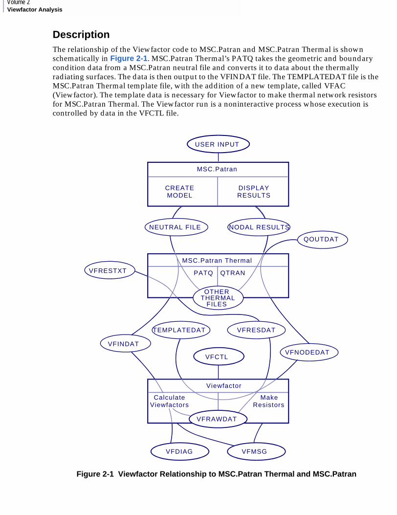
DescriptionThe relationship of the Viewfactor code to MSC.Patran and MSC.Patran Thermal is shown schematically in Figure 2-1. MSC.Patran Thermal’s PATQ takes the geometric and boundary condition data from a MSC.Patran neutral file and converts it to data about the thermally radiating surfaces. The data is then output to the VFINDAT file. The TEMPLATEDAT file is the MSC.Patran Thermal template file, with the addition of a new template, called VFAC (Viewfactor). The template data is necessary for Viewfactor to make thermal network resistors for MSC.Patran Thermal. The Viewfactor run is a noninteractive process whose execution is controlled by data in the VFCTL file.
Figure 2-1 Viewfactor Relationship to MSC.Patran Thermal and MSC.Patran
USER INPUT
VFRESTXT
QOUTDAT
VFINDAT
VFCTL
OTHER THERMAL
FILES
TEMPLATEDAT VFRESDAT
VFNODEDAT
VFRAWDAT
VFMSG VFDIAG
MSC.Patran
CREATE MODEL
DISPLAY RESULTS
MSC.Patran Thermal
PATQ QTRAN
Viewfactor
Make Resistors
Calculate Viewfactors
NEUTRAL FILE NODAL RESULTS
1CHAPTER 2Overview
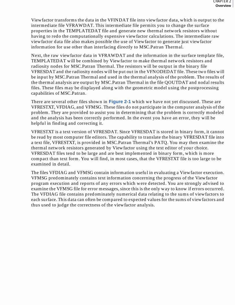
Viewfactor transforms the data in the VFINDAT file into viewfactor data, which is output to the intermediate file VFRAWDAT. This intermediate file permits you to change the surface properties in the TEMPLATEDAT file and generate new thermal network resistors without having to redo the computationally expensive viewfactor calculations. The intermediate raw viewfactor data file also makes possible the use of Viewfactor to generate just viewfactor information for use other than interfacing directly to MSC.Patran Thermal.
Next, the raw viewfactor data in VFRAWDAT and the information in the surface template file, TEMPLATEDAT will be combined by Viewfactor to make thermal network resistors and radiosity nodes for MSC.Patran Thermal. The resistors will be output in the binary file VFRESDAT and the radiosity nodes will be put out in the VFNODEDAT file. These two files will be input by MSC.Patran Thermal and used in the thermal analysis of the problem. The results of the thermal analysis are output by MSC.Patran Thermal in the file QOUTDAT and nodal results files. These files may be displayed along with the geometric model using the postprocessing capabilities of MSC.Patran.
There are several other files shown in Figure 2-1 which we have not yet discussed. These are VFRESTXT, VFDIAG, and VFMSG. These files do not participate in the computer analysis of the problem. They are provided to assist you in determining that the problem is correctly modeled and the analysis has been correctly performed. In the event you have an error, they will be helpful in finding and correcting it.
VFRESTXT is a text version of VFRESDAT. Since VFRESDAT is stored in binary form, it cannot be read by most computer file editors. The capability to translate the binary VFRESDAT file into a text file, VFRESTXT, is provided in MSC.Patran Thermal’s PATQ. You may then examine the thermal network resistors generated by Viewfactor using the text editor of your choice. VFRESDAT files tend to be large and are best implemented in binary form, which is more compact than text form. You will find, in most cases, that the VFRESTXT file is too large to be examined in detail.
The files VFDIAG and VFMSG contain information useful in evaluating a Viewfactor execution. VFMSG predominately contains text information concerning the progress of the Viewfactor program execution and reports of any errors which were detected. You are strongly advised to examine the VFMSG file for error messages, since this is the only way to know if errors occurred. The VFDIAG file contains predominately numerical data relating to the sums of viewfactors to each surface. This data can often be compared to expected values for the sums of viewfactors and thus used to judge the correctness of the viewfactor analysis.

Volume 2Viewfactor Analysis
2.3 Viewfactor Data and Program FlowThis section describes in a very general manner the internal workings of the Viewfactor code. Strictly speaking, it is not necessary to know this information in order to use Viewfactor. However, by knowing something about Viewfactor’s internal data flow it is easier to understand some of the information needed in order to use Viewfactor. Therefore, while it is not necessary to dwell on the details of this section, it is good to be familiar with it. You may also wish to refer to this section from time to time to refresh your memory or to facilitate your understanding of how some detail of the viewfactor analysis fits into the overall MSC.Patran System Thermal Analysis scheme.
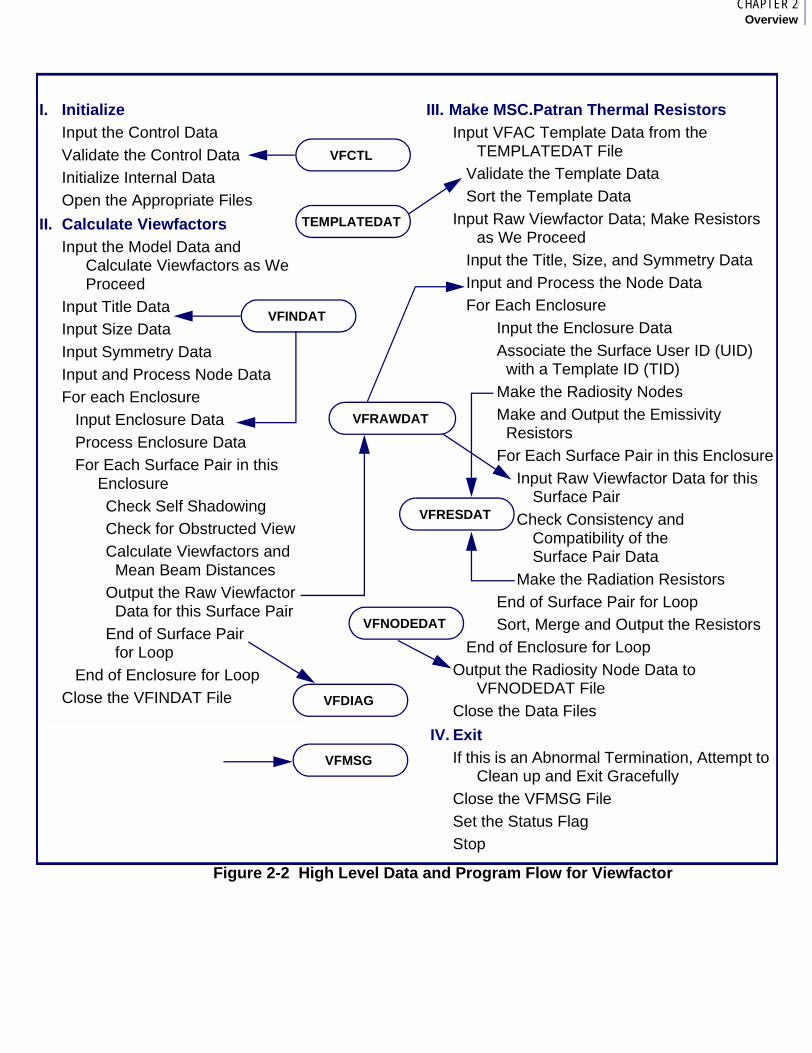
DescriptionFigure 2-2 shows a high level abstraction of the program structure contained in Viewfactor. The program functions are described in outline form, with the level of indentation representing the level of nesting in the program. Data files are shown in ovals with arrows to the general portion of the program where the data is input or output. The file VFMSG receives output throughout the program execution and thus does not have an arrow from a specific portion of the program.
1CHAPTER 2Overview
Figure 2-2 High Level Data and Program Flow for Viewfactor
I. Initialize Input the Control DataValidate the Control DataInitialize Internal DataOpen the Appropriate Files
II. Calculate Viewfactors Input the Model Data and
Calculate Viewfactors as We Proceed
Input Title DataInput Size DataInput Symmetry DataInput and Process Node DataFor each Enclosure
Input Enclosure DataProcess Enclosure DataFor Each Surface Pair in this
EnclosureCheck Self ShadowingCheck for Obstructed ViewCalculate Viewfactors and
Mean Beam DistancesOutput the Raw Viewfactor
Data for this Surface PairEnd of Surface Pair
for LoopEnd of Enclosure for Loop
Close the VFINDAT File
III. Make MSC.Patran Thermal ResistorsInput VFAC Template Data from the
TEMPLATEDAT FileValidate the Template DataSort the Template Data
Input Raw Viewfactor Data; Make Resistors as We Proceed
Input the Title, Size, and Symmetry DataInput and Process the Node DataFor Each Enclosure
Input the Enclosure DataAssociate the Surface User ID (UID)
with a Template ID (TID)Make the Radiosity NodesMake and Output the Emissivity
ResistorsFor Each Surface Pair in this Enclosure
Input Raw Viewfactor Data for this Surface Pair
Check Consistency and Compatibility of the Surface Pair Data
Make the Radiation ResistorsEnd of Surface Pair for LoopSort, Merge and Output the Resistors
End of Enclosure for LoopOutput the Radiosity Node Data to
VFNODEDAT FileClose the Data Files
IV. ExitIf this is an Abnormal Termination, Attempt to
Clean up and Exit GracefullyClose the VFMSG FileSet the Status FlagStop
TEMPLATEDAT
VFCTL
VFINDAT
VFRAWDAT
VFRESDAT
VFNODEDAT
VFDIAG
VFMSG
Volume 2Viewfactor Analysis
The execution of Viewfactor is controlled by parameters in the control file VFCTL. These parameters serve three general purposes:
1. Set program parameters, such as the value of the parameter used for convergence checking.
2. Specify file names other than the default names for the data files.
3. Control which parts of the Viewfactor program are executed and subsequently which input data files are required and which output data files are created.
The third function of program control is described here. All of these functions are described in more detail in Viewfactor Execution From MSC.Patran Thermal (p. 89).
Referring to Figure 2-2, you should be able to identify the following program parts:
Parts I and IV are always executed. Through the use of a parameter in the VFCONTROL file you may cause any one of three execution modes to occur.
Part I Initialize.
Part II Calculate Viewfactors.
Part III Make MSC.Patran Thermal Resistors.
Part IV Exit from the Viewfactor program structure.
MODE 1 In the first mode, all of the Parts I through IV are executed. The required data input is a VFCTL file, a VFINDAT file, and a TEMPLATEDAT file. The output produced is a VFRESDAT file, a VFNODEDAT file, a VFRAWDAT file, a VFDIAG file, and a VFMSG file. This mode takes in the geometric description of the radiating surfaces and their MSC.Patran Thermal surface template data and creates as output resistor network data for MSC.Patran Thermal. Also created as output for possible later use (see the description of the third mode below) is the raw viewfactor data. Diagnostic data is also output.
1CHAPTER 2Overview
MODE 2 In the second mode, only Parts I, II, and IV are executed. Part III (Make MSC.Patran Thermal Resistors) is not executed and thus no thermal network data is generated. The TEMPLATEDAT file is not required for this mode, although no harm will be caused by its presence. The required data input is a VFCTL file and a VFINDAT file. The output produced is a raw viewfactor file, VFRAWDAT, and the diagnostic files VFDIAG and VFMSG. The VFRAWDAT file produced here may be used in the third mode described in the next paragraph. The second mode is useful if you only want to generate viewfactor data and do not care about the MSC.Patran Thermal network resistors. It is also useful if you do not yet have the TEMPLATEDAT file describing the surface properties and wish to begin the viewfactor calculations. You must take care to make sure that the thermal radiation problem described in the VFINDAT file and the property data identified in the yet to be created TEMPLATEDAT file are compatible. This is described in more detail in Compatibility Requirements for Model and VFAC Templates (p. 75) and Introduction (p. 130). The intermediate file VFRAWDAT and the TEMPLATEDAT file may be combined to make the thermal network resistors at some later time by using the third mode.
MODE 3 In the third mode, only Parts I, III, and IV are executed. Part II, (Calculate Viewfactors) is not executed and thus there must already be in existence and available to the program a data file of raw viewfactor data, VFRAWDAT. This mode also requires a TEMPLATEDAT file of surface data for the MSC.Patran Thermal resistors that will be created. The VFCTL file is also input in this mode. The output created here is the thermal resistor network for the radiating surfaces, contained in the files VFRESDAT and VFNODEDAT, and the diagnostic data contained in the files VFDIAG and VFMSG.
This third mode allows you to change the surface property definition by changing the information contained in the TEMPLATEDAT file. Then run this mode of the Viewfactor program again. Note that in this way you may generate a new and different thermal resistor network simply by changing the TEMPLATEDAT file. You do not have to rerun the computationally expensive viewfactor calculations which were already performed in the first or second modes described above. This provides great savings of computer time in cases where the geometry does not change, but you wish to run two or more thermal analyses using different radiative surface properties. It is also useful for performing initial analysis using simpler material properties (e.g., constant properties). Once the analyst is satisfied that the problem is correctly modeled, the material properties may be changed to more closely represent reality (e.g., temperature dependent properties). By submitting simpler, computationally faster models for preliminary analysis the analyst can optimize the use of available computer resources and improve overall performance.
When using this mode you must take special care to define the radiating surfaces in such a way that they are capable of supporting all of the various material property definitions you plan to attach to each surface in the future. This method is described in more detail in MSC.Patran Thermal TEMPLATEDAT Files for Surface Property Description (p. 60) and Introduction (p. 130).
Volume 2Viewfactor Analysis
2.4 Summary of the Analysis Cycle for a Thermal Radiation ProblemThermal phenomena tend to be complex physical processes and the analysis of these processes by digital computer is equally complex. The tools provided by MSC.Software Corporation in the form of MSC.Patran and P⁄ THERMAL provide advanced capabilities to model some very complex thermal problems. While great effort has been taken to make the tools simple and easy to use, the very complexity of the thermal analysis problem necessitates some degree of complexity in the software provided to perform the analysis. This section provides an overview of the generic thermal analysis cycle using MSC.Patran and MSC.Patran Thermal. Since this Guide deals with Viewfactor analysis, this summary emphasizes parts of the cycle peculiar to the analysis of a problem containing thermal radiation.
Problem DefinitionThe first step is to define the problem. This includes identifying the geometry, boundary conditions, materials, material properties and approximations to be used in the analysis. You may find it useful and efficient to outline the entire analysis procedure as it pertains to the problem at hand. This should help avoid unpleasant surprises later on. It also ensures that all the steps in a complex process are followed.
General PreprocessingThis step involves creating or inputting the geometric model, creating a finite element mesh on the model, and assigning boundary conditions and material identifications, in MSC.Patran. This step requires close coordination with the next step, General MSC.Patran Thermal Preparation, so that the boundary conditions and material properties identified in MSC.Patran correspond to material definitions and boundary conditions in the supporting MSC.Patran Thermal files. These activities and entities are described more fully in the MSC.Patran Thermal User’s Guide. Planning at this stage of the analysis is important if you wish to be able to easily change boundary conditions and/or material property definitions in the future.
General MSC.Patran Thermal PreparationThe model of the thermal analysis problem built with the MSC.Patran preprocessor generally has only identification numbers attached to boundary conditions and material properties. These identification numbers are used by the MSC.Patran Thermal module to point into various databases and files for the actual data describing the boundary condition or material property. If these files do not already exist, they must be created. Details concerning these files are contained in the MSC.Patran Thermal User’s Guide.

2CHAPTER 2Overview
Thermal Radiation Specific PreprocessingThermal radiation problems analyzed with the MSC.Patran System of products require some specific preprocessing in MSC.Patran. You must identify the material surfaces which are participating in the radiation interchange and identify the radiative properties of these material surfaces. The VFAC LBC form has been introduced into MSC.Patran specifically to facilitate the modeling of thermal radiation problems. The VFAC form provides support for basic thermal radiation boundary conditions, for participating absorbing and emitting media between surfaces, for identifying convex surfaces which cannot radiate to themselves directly, for identifying surfaces that are not obstructions, and for radiation to an ambient node. This MSC.Patran form is described in detail in Advanced Features of the VFAC Boundary Condition (p. 48).
In support of these modeling capabilities, you will also need to enter data into the MSC.Patran Thermal files for the surface emissivity properties and the participating media (if any) extinction or transmissivity properties, including in both cases waveband data if applicable. This data is typically entered into the MSC.Patran Thermal TEMPLATEDAT, MATDAT, and MICRODAT files. These files and data relevant to a thermal radiation problem will be briefly described in MSC.Patran Thermal TEMPLATEDAT Files for Surface Property Description (p. 60). For full details on these files, refer to the MSC.Patran Thermal User’s Guide.
Facilities have also been programmed into MSC.Patran Thermal and Viewfactor to accept and process information about symmetry occurring in the thermal analysis problem. Problem symmetry is also input in MSC.Patran at this stage of the analysis cycle. The use of symmetry in thermal radiation problems is described in more detail in Symmetry as Applied to the Model and Viewfactor Radiation Exchange (p. 77).
Preparation for Viewfactor AnalysisAfter the model of the problem to be analyzed has been prepared in MSC.Patran and the required supporting MSC.Patran Thermal files have been created, there are two steps to prepare the problem for processing by Viewfactor. These are:
1. Translate the model description contained in the MSC.Patran neutral file to the data and form required for the Viewfactor input file VFINDAT, and
2. Create a VFCTL file which will direct the execution of Viewfactor.
The translation of the MSC.Patran neutral file is done using a menu pick from MSC.Patran Thermal’s PATQ menu and is described in detail in Preparation for Analysis (Ch. 4). The VFCTL file is typically created using your editor. It is about 20 lines of identifying keywords and associated parameter values. This file is described in Viewfactor Execution From MSC.Patran Thermal (p. 89).
Note: The VFCTL file is automatically created when the analysis is submitted from the Analysis form in MSC.Patran.

Volume 2Viewfactor Analysis
Viewfactor AnalysisViewfactor will usually be executed as a noninteractive batch process. Merely invoke the command procedure to submit Viewfactor and its control file, VFCTL, for execution, or select “Execute Viewfactor Analysis” in the Analysis / Submit Options form.
Since Viewfactor analysis tends to be computationally expensive, review all aspects of the model carefully before beginning the viewfactor analysis. This will help to minimize the number of Viewfactor analyses submitted with incorrect or incomplete data. Viewfactor has some data checking and error detection capabilities, but it cannot detect all user errors. The procedure for submitting a Viewfactor job is described in detail in Submitting a Viewfactor Job for Analysis (p. 108).
Viewfactor will create a number of output files. The files created depend on some parameters in the VFCTL file. The various files created as Viewfactor output are described in Viewfactor Data and Program Flow (p. 16) and Output Created by a Viewfactor Execution (p. 111). When the viewfactor analysis is completed, the Viewfactor diagnostic files, VFDIAG and VFMSG, should be reviewed for acceptable diagnostic data values and possible error messages, as described in Reviewing the Viewfactor Output (p. 114).
Post Viewfactor AnalysisAfter the Viewfactor analysis is complete and the rest of the MSC.Patran Thermal input files are complete, the user is ready to perform the thermal network analysis using MSC.Patran Thermal. Viewfactor will have created two files to which MSC.Patran Thermal must be given access. These are the radiation resistor file, VFRESDAT, and the radiosity node file, VFNODEDAT. This access is usually provided by giving MSC.Patran Thermal the names of these files through the MSC.Patran Thermal QINDAT file. The QINDAT file is described in the MSC.Patran Thermal User’s Guide. The particular aspects of the QINDAT file relevant to the viewfactor analysis and the Viewfactor files VFRESDAT and VFNODEDAT are described in Interface From Viewfactor to MSC.Patran Thermal (p. 123).
At this point in the analysis cycle you may also translate the binary radiation resistor data file, VFRESDAT, into a text file which you may examine. This capability is provided by a menu pick in MSC.Patran Thermal’s PATQ and is described in Interface From Viewfactor to MSC.Patran Thermal (p. 123). This text file has no other purpose in the analysis. It is provided merely for your convenience.
The viewfactor portion of the analysis is now complete. The remaining steps in the analysis cycle all concern general thermal analysis.
MSC.Patran Thermal AnalysisThe procedure for submitting a MSC.Patran Thermal analysis is described in the MSC.Patran Thermal User’s Guide. Briefly, the process involves generating some FORTRAN source code for the particular problem, compiling the new source code, linking with the MSC.Patran Thermal QTRAN run-time library, and submitting the job for execution. The results of the thermal analysis will be contained in the MSC.Patran Thermal QOUTDAT file and in nodal results files for use with the MSC.Patran postprocessing tools.

2CHAPTER 2Overview
PostprocessingThe capabilities of MSC.Patran and the MSC.Patran Thermal interface permit analysis results to be displayed and examined quickly and efficiently. For more information about thermal results postprocessing, refer to the MSC.Patran Thermal User’s Guide. Refer to the MSC.Patran Reference Manual for general postprocessing information.
RefinementsAfter examining the analysis results, you may be satisfied with the analysis, in which case this analysis cycle terminates. You may wish to refine or modify the computer model of the problem and perform the analysis again, in which case the analysis cycle starts over and repeats itself as applicable.

Volume 2Viewfactor Analysis
MSC.Patran Thermal User’s Guide, Volume 2: Viewfactor Analysis
CHAPTER
3 Model Creation for a Thermal Radiation Problem
■ Purpose
■ Radiation Enclosure Concept
■ Surface Orientation in MSC.Patran
■ Specifying Radiation Boundary Conditions Using MSC.Patran Reference Manual (VFAC Boundary Condition)
■ Advanced Features of the VFAC Boundary Condition
■ Relationship of VFAC LBC Data to VFINDAT File Data
■ MSC.Patran Thermal TEMPLATEDAT Files for Surface Property Description
■ Compatibility Requirements for Model and VFAC Templates
■ Symmetry as Applied to the Model and Viewfactor Radiation Exchange
Volume 2Viewfactor Analysis
3.1 PurposeThis chapter presents the concepts, processes, and commands that describe the thermal radiation specific attributes of heat transfer analysis problems being modeled in the MSC.Patran System. Most of this chapter deals with preprocess model building in MSC.Patran.
The concept of radiation enclosure is specific to thermal radiation analysis and is described in Radiation Enclosure Concept (p. 27). The concept of surface orientation, while not unique to thermal radiation analysis, has not been introduced previously in MSC.Software Corporation thermal analysis tools, and is described in Surface Orientation in MSC.Patran (p. 35). Specifying Radiation Boundary Conditions Using MSC.Patran Reference Manual (VFAC Boundary Condition) (p. 43) and Advanced Features of the VFAC Boundary Condition (p. 48) deal with identifying the radiative boundary conditions and other associated information using the MSC.Patran Radiation Boundary condition.
Relationship of VFAC LBC Data to VFINDAT File Data (p. 59) explains the relationship of the Viewfactor LBC form to the data in the VFINDAT input data file for Viewfactor. MSC.Patran Thermal TEMPLATEDAT Files for Surface Property Description (p. 60) and Compatibility Requirements for Model and VFAC Templates (p. 76) discuss the MSC.Patran Thermal TEMPLATEDAT file and the associated VFAC template data. In the last section of this chapter, page 78, the role of symmetry in thermal radiation problems is discussed. The method for specifying the existence and type of symmetry in a problem is presented.
Some sophisticated thermal analysis tools have been provided and thus this chapter contains a large amount of information. Take the time to understand all of the capabilities of the tools available here. This will enable you to make informed decisions regarding how to model the thermal radiation phenomena at hand and choose the appropriate tools for the analysis.
You must understand the concept of radiation enclosure, Radiation Enclosure Concept (p. 27). If you wish to model materials or media with wavelength dependent properties, then Surface Orientation in MSC.Patran (p. 35) must be understood. Specifying Radiation Boundary Conditions Using MSC.Patran Reference Manual (VFAC Boundary Condition) (p. 43) deals with basic radiative boundary conditions, while Advanced Features of the VFAC Boundary Condition (p. 48) deals with move advanced features that enable modeling of participating media, radiation to ambient nodes, and methods for reducing CPU time required for a Viewfactor analysis.
If you are also responsible for the accompanying MSC.Patran Thermal analysis, then MSC.Patran Thermal TEMPLATEDAT Files for Surface Property Description (p. 60) andCompatibility Requirements for Model and VFAC Templates (p. 76) regarding the TEMPLATEDAT files and VFAC templates are strongly recommended. Be cautious using symmetry in thermal radiation problems, since the thermal radiation boundary conditions have subtle ways of making what appears to be a symmetric problem actually nonsymmetric. However, if you must make use of symmetry, Symmetry as Applied to the Model and Viewfactor Radiation Exchange (p. 78) should be thoroughly mastered.

2CHAPTER 3Model Creation for a Thermal Radiation Problem
3.2 Radiation Enclosure ConceptThe radiation enclosure concept is fundamental to the analysis of thermal radiation problems and also to the techniques used to model the problems in Viewfactor and MSC.Patran Thermal. Therefore, it is important to understand the concept, not only as it is classically applied to thermal radiation problems, but also as it is used in creating the computer model of the thermal radiation phenomena.
Definition of EnclosureFor our purposes, an enclosure is a collection of thermally radiating surfaces which have the potential to see each other (radiate to each other), along with open areas which can potentially be seen by the surfaces and participating media or ambient nodes associated with these surfaces. From this definition you may infer that there are a large number of enclosures possible in even a simple model. It is up to you to select appropriate enclosures for the particular thermal analysis problem at hand. In most cases, appropriate choices of enclosures are natural and obvious from the model geometry.
Surfaces in different enclosures do not have the potential to radiate to each other. In addition, a surface in one enclosure does not have the ability to obstruct the view between a pair of surfaces in another enclosure. These properties of enclosures are exploited in the Viewfactor program to reduce the CPU time required to analyze the viewfactor problem. Surfaces not in an enclosure need not be considered as potential obstructions for that enclosure. Surface pairs that are not in the same enclosure need not have calculations done for them.
The enclosures are also used for defining portions of the model over which the viewfactors from one surface to all other surfaces it sees are summed. These sums have two uses:
1. For diagnostic purposes, and
2. To determine the viewfactor to that portion of the enclosure that is not represented by real surfaces, but instead is open to space.
The Enclosure IDEnclosures are made distinct by giving each different one a unique identification number. This ID number is associated with all of the surfaces in its enclosure. The enclosure ID is assigned in the VFAC LBC form as described in Viewfactor (p. 118) in the MSC.Patran Thermal User’s Guide, Volume 1: Thermal/Hydraulic Analysis.

Volume 2Viewfactor Analysis
Wavebands and EnclosuresWavebands are used when the thermal radiative material properties depend on the wavelength of the radiation (they may also depend on time and temperature). The concept of wavebands and their proper use in modeling the thermal analysis problem are explained in MSC.Patran Thermal TEMPLATEDAT Files for Surface Property Description (p. 60).
If you do not need to use spectrally dependent material properties to adequately model the problem, then this subsection need not be understood. Note, however that you will need to understand this subsection in order to understand all of the examples in the next subsection, Examples of the Use of Enclosures (p. 29).
Enclosures and wavebands (see page 60) have a special relationship. The wavebands associated with each surface in an enclosure must match exactly the wavebands of every other surface in that enclosure which the first surface can see.
This holds true when every surface in the enclosure has the same wavebands. It is recommended that all surfaces within an enclosure have the same wavebands. For two surfaces in an enclosure, if the surfaces can see each other and the wavebands are not identical, then a fatal error will occur when you attempt to make radiation resistors for the model. This error cannot be detected until after the viewfactors are calculated (the most CPU intensive part of the Viewfactor analysis). It is a mistake that you should avoid so that you do not have to redo the viewfactor calculations.
For the wavebands associated with two surfaces to be identical is meant:
• The number of wavebands for each surface must be the same, and
• The lower limit of each waveband on each surface must be the same and
• The upper limit of each waveband on each surface must be the same and
• The wavebands for each surface must be input in the same order in the TEMPLATEDAT file.
2CHAPTER 3Model Creation for a Thermal Radiation Problem
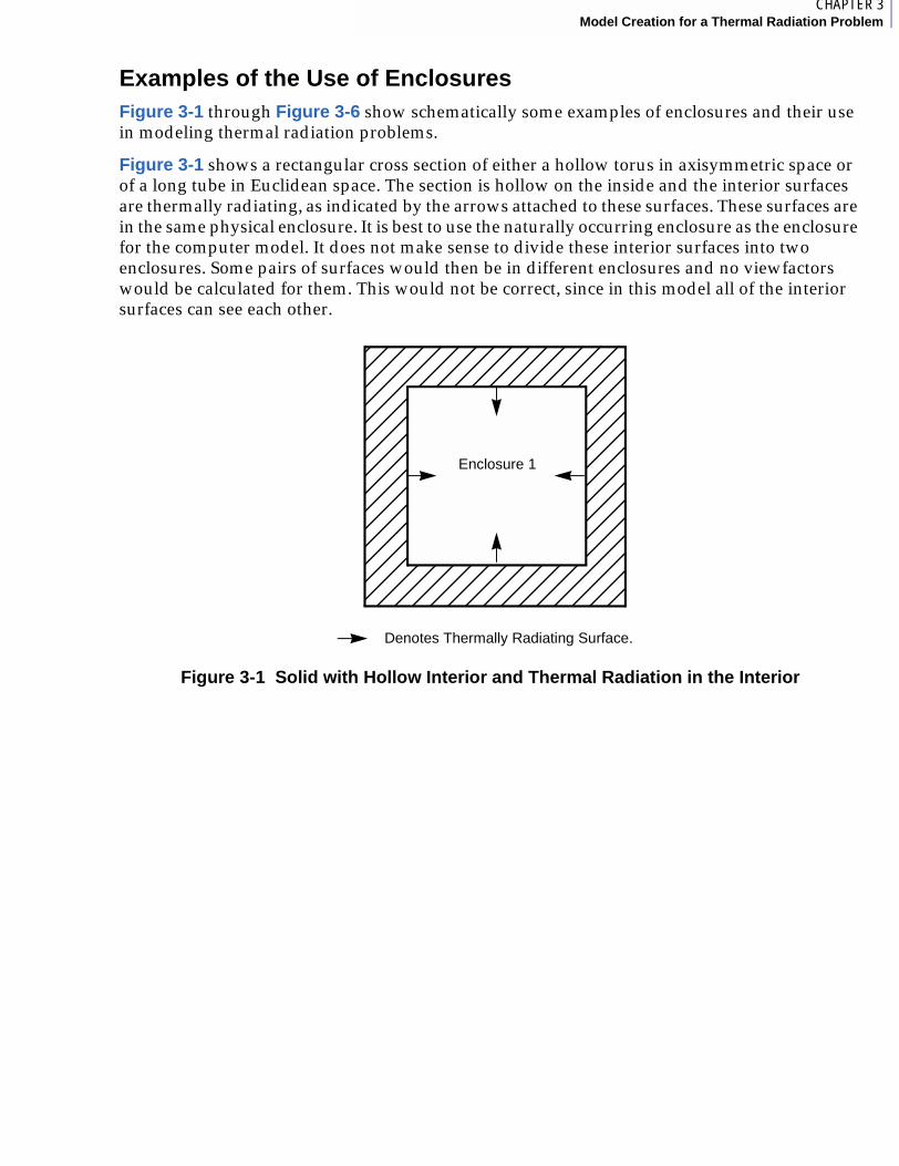
Examples of the Use of Enclosures Figure 3-1 through Figure 3-6 show schematically some examples of enclosures and their use in modeling thermal radiation problems.
Figure 3-1 shows a rectangular cross section of either a hollow torus in axisymmetric space or of a long tube in Euclidean space. The section is hollow on the inside and the interior surfaces are thermally radiating, as indicated by the arrows attached to these surfaces. These surfaces are in the same physical enclosure. It is best to use the naturally occurring enclosure as the enclosure for the computer model. It does not make sense to divide these interior surfaces into two enclosures. Some pairs of surfaces would then be in different enclosures and no viewfactors would be calculated for them. This would not be correct, since in this model all of the interior surfaces can see each other.
Figure 3-1 Solid with Hollow Interior and Thermal Radiation in the Interior
Enclosure 1
Denotes Thermally Radiating Surface.
Volume 2Viewfactor Analysis
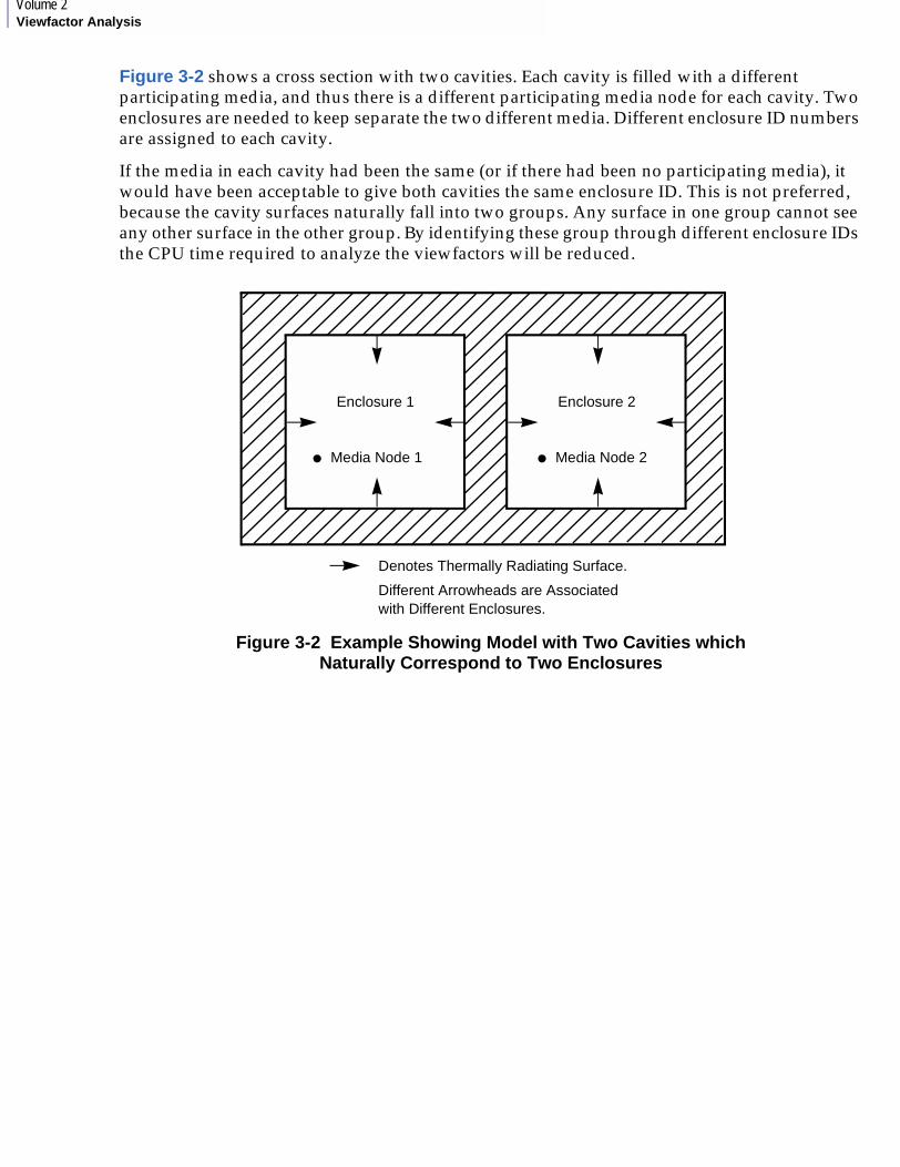
Figure 3-2 shows a cross section with two cavities. Each cavity is filled with a different participating media, and thus there is a different participating media node for each cavity. Two enclosures are needed to keep separate the two different media. Different enclosure ID numbers are assigned to each cavity.
If the media in each cavity had been the same (or if there had been no participating media), it would have been acceptable to give both cavities the same enclosure ID. This is not preferred, because the cavity surfaces naturally fall into two groups. Any surface in one group cannot see any other surface in the other group. By identifying these group through different enclosure IDs the CPU time required to analyze the viewfactors will be reduced.
Figure 3-2 Example Showing Model with Two Cavities which Naturally Correspond to Two Enclosures
Enclosure 1
Denotes Thermally Radiating Surface.
Different Arrowheads are Associated with Different Enclosures.
Enclosure 2
• Media Node 1 • Media Node 2
3CHAPTER 3Model Creation for a Thermal Radiation Problem
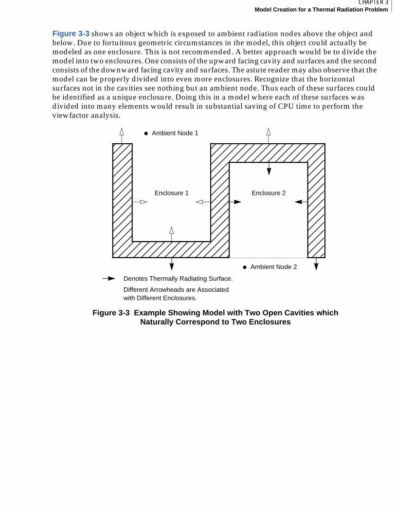
Figure 3-3 shows an object which is exposed to ambient radiation nodes above the object and below. Due to fortuitous geometric circumstances in the model, this object could actually be modeled as one enclosure. This is not recommended. A better approach would be to divide the model into two enclosures. One consists of the upward facing cavity and surfaces and the second consists of the downward facing cavity and surfaces. The astute reader may also observe that the model can be properly divided into even more enclosures. Recognize that the horizontal surfaces not in the cavities see nothing but an ambient node. Thus each of these surfaces could be identified as a unique enclosure. Doing this in a model where each of these surfaces was divided into many elements would result in substantial saving of CPU time to perform the viewfactor analysis.
Figure 3-3 Example Showing Model with Two Open Cavities which Naturally Correspond to Two Enclosures
• Ambient Node 1
• Ambient Node 2
Enclosure 1 Enclosure 2
Denotes Thermally Radiating Surface.
Different Arrowheads are Associated with Different Enclosures.
Volume 2Viewfactor Analysis
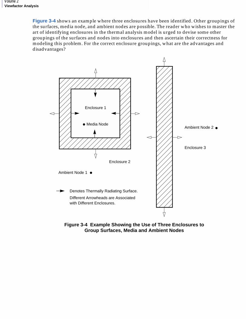
Figure 3-4 shows an example where three enclosures have been identified. Other groupings of the surfaces, media node, and ambient nodes are possible. The reader who wishes to master the art of identifying enclosures in the thermal analysis model is urged to devise some other groupings of the surfaces and nodes into enclosures and then ascertain their correctness for modeling this problem. For the correct enclosure groupings, what are the advantages and disadvantages?
Figure 3-4 Example Showing the Use of Three Enclosures to Group Surfaces, Media and Ambient Nodes
Enclosure 1
Ambient Node 2 •
Enclosure 2
Enclosure 3
Ambient Node 1 •
• Media Node
Denotes Thermally Radiating Surface.
Different Arrowheads are Associated with Different Enclosures.
3CHAPTER 3Model Creation for a Thermal Radiation Problem
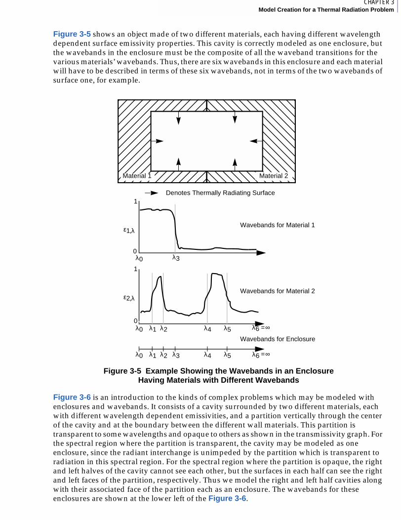
Figure 3-5 shows an object made of two different materials, each having different wavelength dependent surface emissivity properties. This cavity is correctly modeled as one enclosure, but the wavebands in the enclosure must be the composite of all the waveband transitions for the various materials’ wavebands. Thus, there are six wavebands in this enclosure and each material will have to be described in terms of these six wavebands, not in terms of the two wavebands of surface one, for example.
Figure 3-5 Example Showing the Wavebands in an Enclosure Having Materials with Different Wavebands
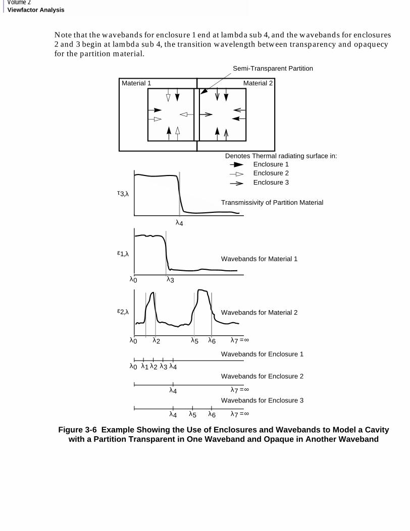
Figure 3-6 is an introduction to the kinds of complex problems which may be modeled with enclosures and wavebands. It consists of a cavity surrounded by two different materials, each with different wavelength dependent emissivities, and a partition vertically through the center of the cavity and at the boundary between the different wall materials. This partition is transparent to some wavelengths and opaque to others as shown in the transmissivity graph. For the spectral region where the partition is transparent, the cavity may be modeled as one enclosure, since the radiant interchange is unimpeded by the partition which is transparent to radiation in this spectral region. For the spectral region where the partition is opaque, the right and left halves of the cavity cannot see each other, but the surfaces in each half can see the right and left faces of the partition, respectively. Thus we model the right and left half cavities along with their associated face of the partition each as an enclosure. The wavebands for these enclosures are shown at the lower left of the Figure 3-6.
Denotes Thermally Radiating Surface
Wavebands for Material 1
Wavebands for Material 2
Wavebands for Enclosure
λ0 λ30
1
ε1,λ
0
1
ε2,λ
λ0 λ1 λ2 λ4 λ5 λ6
λ0 λ1 λ2 λ3 λ4 λ5 λ6
=∞
=∞
Material 1 Material 2
Volume 2Viewfactor Analysis
Note that the wavebands for enclosure 1 end at lambda sub 4, and the wavebands for enclosures 2 and 3 begin at lambda sub 4, the transition wavelength between transparency and opaquecy for the partition material.
Figure 3-6 Example Showing the Use of Enclosures and Wavebands to Model a Cavity with a Partition Transparent in One Waveband and Opaque in Another Waveband
Denotes Thermal radiating surface in:
λ0 λ3
ε1,λ
ε2,λ
λ2
λ4
Semi-Transparent Partition
Material 1
Enclosure 1
Transmissivity of Partition Material
λ0 λ1 λ2 λ3
λ0
λ5 λ6 =∞
τ3,λ
Wavebands for Material 1
Wavebands for Material 2
Wavebands for Enclosure 1
Wavebands for Enclosure 2
Wavebands for Enclosure 3
λ4
λ4
λ7
=∞λ7
λ5 λ6 =∞λ7
λ4
Material 2
Enclosure 2Enclosure 3
3CHAPTER 3Model Creation for a Thermal Radiation Problem
3.3 Surface Orientation in MSC.PatranMSC.Patran does not check for consistently oriented surfaces in two-dimensional entities such as patches and quadrilateral elements. Properly oriented surfaces are required for correct modeling of 2-D XY and 2-D axisymmetric thermal radiation models. Since MSC.Patran does not ensure consistent surface orientation, the user must assume this responsibility. Failure to do so will result in erroneous models.
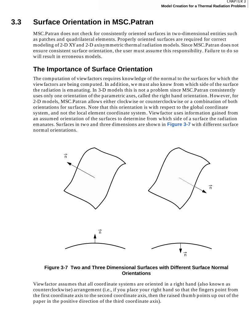
The Importance of Surface OrientationThe computation of viewfactors requires knowledge of the normal to the surfaces for which the viewfactors are being computed. In addition, we must also know from which side of the surface the radiation is emanating. In 3-D models this is not a problem since MSC.Patran consistently uses only one orientation of the parametric axes, called the right hand orientation. However, for 2-D models, MSC.Patran allows either clockwise or counterclockwise or a combination of both orientations for surfaces. Note that this orientation is with respect to the global coordinate system, and not the local element coordinate system. Viewfactor uses information gained from an assumed orientation of the surfaces to determine from which side of a surface the radiation emanates. Surfaces in two and three dimensions are shown in Figure 3-7 with different surface normal orientations.
Figure 3-7 Two and Three Dimensional Surfaces with Different Surface Normal Orientations
Viewfactor assumes that all coordinate systems are oriented in a right hand (also known as counterclockwise) arrangement (i.e., if you place your right hand so that the fingers point from the first coordinate axis to the second coordinate axis, then the raised thumb points up out of the paper in the positive direction of the third coordinate axis).
n
n
n
n
Volume 2Viewfactor Analysis
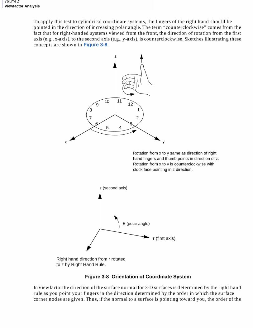
To apply this test to cylindrical coordinate systems, the fingers of the right hand should be pointed in the direction of increasing polar angle. The term “counterclockwise” comes from the fact that for right-handed systems viewed from the front, the direction of rotation from the first axis (e.g., x-axis), to the second axis (e.g., y-axis), is counterclockwise. Sketches illustrating these concepts are shown in Figure 3-8.
Figure 3-8 Orientation of Coordinate System
InViewfactorthe direction of the surface normal for 3-D surfaces is determined by the right hand rule as you point your fingers in the direction determined by the order in which the surface corner nodes are given. Thus, if the normal to a surface is pointing toward you, the order of the
Rotation from x to y same as direction of righthand fingers and thumb points in direction of z.Rotation from x to y is counterclockwise withclock face pointing in z direction.
Right hand direction from r rotated to z by Right Hand Rule.
r (first axis)
z (second axis)
θ (polar angle)
z
yx
12
62
1
11
345
7
89
10
3CHAPTER 3Model Creation for a Thermal Radiation Problem
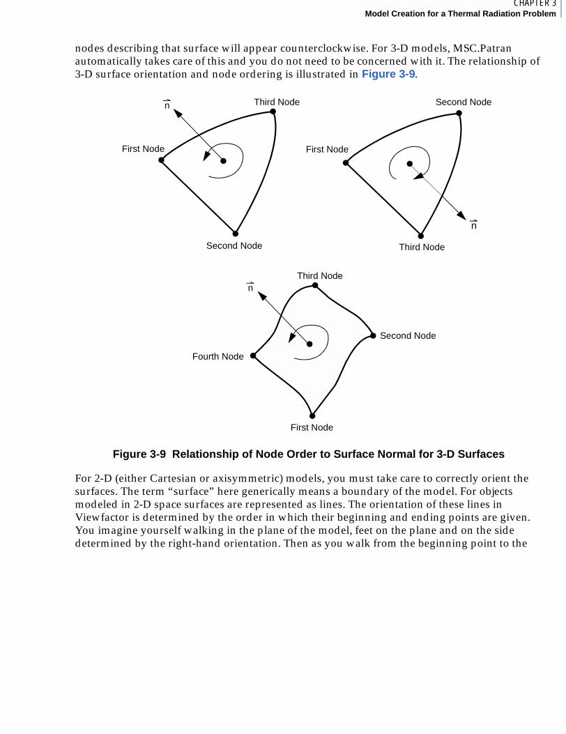
nodes describing that surface will appear counterclockwise. For 3-D models, MSC.Patran automatically takes care of this and you do not need to be concerned with it. The relationship of 3-D surface orientation and node ordering is illustrated in Figure 3-9.
Figure 3-9 Relationship of Node Order to Surface Normal for 3-D Surfaces
For 2-D (either Cartesian or axisymmetric) models, you must take care to correctly orient the surfaces. The term “surface” here generically means a boundary of the model. For objects modeled in 2-D space surfaces are represented as lines. The orientation of these lines in Viewfactor is determined by the order in which their beginning and ending points are given. You imagine yourself walking in the plane of the model, feet on the plane and on the side determined by the right-hand orientation. Then as you walk from the beginning point to the
n
n
n
Third Node Second Node
First Node
Third Node
Third Node
Second Node
Second Node
First Node
First Node
Fourth Node
Volume 2Viewfactor Analysis
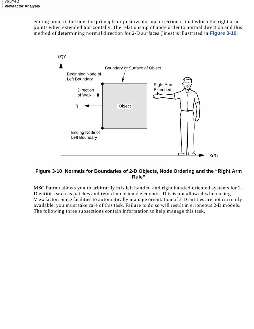
ending point of the line, the principle or positive normal direction is that which the right arm points when extended horizontally. The relationship of node order to normal direction and this method of determining normal direction for 2-D surfaces (lines) is illustrated in Figure 3-10.
Figure 3-10 Normals for Boundaries of 2-D Objects, Node Ordering and the “Right Arm Rule”
MSC.Patran allows you to arbitrarily mix left handed and right handed oriented systems for 2-D entities such as patches and two-dimensional elements. This is not allowed when using Viewfactor. Since facilities to automatically manage orientation of 2-D entities are not currently available, you must take care of this task. Failure to do so will result in erroneous 2-D models. The following three subsections contain information to help manage this task.
n
(Z)Y
X(R)
Boundary or Surface of Object
Beginning Node ofLeft Boundary
Directionof Walk
Ending Node ofLeft Boundary
Object
Right ArmExtended
3CHAPTER 3Model Creation for a Thermal Radiation Problem
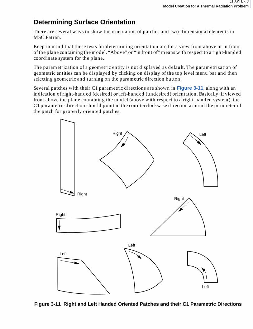
Determining Surface OrientationThere are several ways to show the orientation of patches and two-dimensional elements in MSC.Patran.
Keep in mind that these tests for determining orientation are for a view from above or in front of the plane containing the model. “Above” or “in front of” means with respect to a right-handed coordinate system for the plane.
The parametrization of a geometric entity is not displayed as default. The parametrization of geometric entities can be displayed by clicking on display of the top level menu bar and then selecting geometric and turning on the parametric direction button.
Several patches with their C1 parametric directions are shown in Figure 3-11, along with an indication of right-handed (desired) or left-handed (undesired) orientation. Basically, if viewed from above the plane containing the model (above with respect to a right-handed system), the C1 parametric direction should point in the counterclockwise direction around the perimeter of the patch for properly oriented patches.
Figure 3-11 Right and Left Handed Oriented Patches and their C1 Parametric Directions
Right
Right
Right
Right
Left
Left
Left
Left

Volume 2Viewfactor Analysis
The next test may be used to determine a patch’s orientation. They are not recommended because they do not conform to the engineering and mathematical standards for surface orientation. These tests are based on the order of the corner grid IDs for the patch and on the order of the edges of the patch. MSC.Patran specifies the corner grid and edge order of right hand oriented patches to be clockwise, whereas most users will be familiar with the usual counterclockwise orientation.
The patch corner grid ordering may be shown by clicking on geometry in MSC.Patran and selecting Action: show, Object: surface, Method: attribute and selecting the surface. When the spreadsheet comes up, click on the vertices button to see the corner grids and their order. Look at the graphics window to see if the grids in this order go clockwise around the patch. If they do, then this is a properly oriented patch.
The ordering of corner grids and edges is shown in Figure 3-12 for various right-handed (properly) and left-handed (improperly) oriented paths.
Figure 3-12 Corner Grid and Patch Edge Ordering for Right- and Left-Hand Oriented Patches
LEFT
1 4
2 3
4
2
31
LEFT
4 3
1 2
3
1
24
RIGHT
2 3
1 4
2
4
31
33
41
2
2
1
4RIGHT
RIGHT 1
4
4
32
1 2
3 RIGHT
2
3
24
3
1
1
4
4
2
1 4
31
32
23
2
4
13
4 1
LEFT
LEFT
RIGHT
2
4
13
4
23
x
x Grid Numbers
Edge Numbers
C1 Parametric Directions

4CHAPTER 3Model Creation for a Thermal Radiation Problem
The orientation of two-dimensional elements (i.e., quadrilaterals and triangles), may be determined by using the element verification menu. Since elements are typically much more numerous than patches, take care to properly orient all patches before beginning to generate elements to ensure that there are no improperly oriented elements.
The commands listed above for determining the element orientation are described fully in the MSC.Patran Reference Manual. Note, however, that the ordering for nodes on a properly oriented element is counterclockwise as is customary in engineering analysis, and that this is opposite of the ordering of corner grids on a properly oriented patch.
Correcting Improper Surface OrientationsImproperly oriented patches may be reversed with the modify action on the geometry menu.
The patch may also be deleted and a new properly oriented patch created in its place, or the patch may be overwritten with a properly oriented patch with the same patch ID. Please see the MSC.Patran Reference Manual for information on the various patch menus.
Elements may be reversed with the AUTOREVERSE option of the NORMALS submenu of the VERIFY action on finite elements form. These forms are all described in the MSC.Patran Reference Manual. You must exercise caution when reversing elements since MSC.Patran may not correctly transform the boundary conditions associated with an element edge when the element is reversed. Other data associated with the element may not be transformed correctly either.
In most cases, if you have left-handed elements, it is recommended that the MSC.Patran finite element entities be deleted. Then the orientation problems should be corrected at the patch level before any finite element entities are generated.
Note: You should not reverse any elements which have LBC element properties associated with it.

Volume 2Viewfactor Analysis
Suggested Practices for Creating Properly Oriented SurfacesIt is important that elements in two-dimensional models (Cartesian and axisymmetric) are correctly oriented. Be aware of the problem and plan carefully to avoid it.
Then, as each patch is made, its orientation should be checked and verified to be correct. Improperly oriented patches should be reversed. This may be done with the modify action of geometry menu.
Carefully check to make sure all patches are properly oriented before beginning to generate the finite elements, finite element properties, and LBCs.
Note: Axisymmetric models only - Since handedness (left- or right-hand rule for orientation) is determined relative to the direction (from the back or from the front) you view the model, righted handedness will appear left handed when viewed from the back. Some commonly used axisymmetric coordinate systems present a view from the back. These systems will require that you use left-handed oriented patches and elements instead of right-handed ones as explained in The Enclosure ID (p. 27), Determining Surface Orientation. To determine which one to use for your axisymmetric coordinate system, perform the following test.
Form the cross product of the r-axis with the z-axis. Use the right-hand rule with your fingers pointing from the r-axis to the z-axis and observe the direction of your thumb. Your thumb will point in the direction of the cross product, either out of the screen or into the screen. If the direction is out of the screen, use right-handed patches and elements. If the direction is into the screen, use left-handed patches and elements.

4CHAPTER 3Model Creation for a Thermal Radiation Problem
3.4 Specifying Radiation Boundary Conditions Using MSC.Patran Reference Manual (VFAC Boundary Condition)The MSC.Patran Viewfactor Loads/BCs option was specifically implemented in MSC.Patran, under the MSC.Patran Thermal preference, to provide support for Viewfactor thermal radiation problems. Basic features of the form are described in this section. Advanced features are described in the following section.
Purpose of the Viewfactor FormThe Viewfactor form is used:
1. To identify surfaces in the model which will participate in thermal radiation interchange;
2. For these surfaces to identify certain properties relevant to thermal radiation transfer;
3. To provide information on radiation enclosures, participating media nodes, ambient nodes, convex surfaces, and nonobstructing surfaces. The surface properties are identified only by a pointer to a VFAC template ID, on the VFAC LBC input data form. This template ID points to material property data in the MSC.Patran Thermal data files. It must correspond to a template ID number, TID, in the template data file, TEMPLATEDAT.
Volume 2Viewfactor Analysis
Form for the VFAC LBCThis is a technical description of the Viewfactor form. For more information, refer to Viewfactor (p. 118) in the MSC.Patran Thermal User’s Guide, Volume 1: Thermal/Hydraulic Analysis.
Input Data for the Viewfactor Form
Input Data Description
VFAC
TEMPLATE ID
The user function ID, UID, identifies the VFAC template in P⁄ THERMAL’s TEMPLATEDAT file which will be used to identify the material properties associated with this surface. These properties include surface emissivity and participating media transmissivity data. This parameter is required and is entered as an integer. In MSC.Patran Thermal and Viewfactor only positive UIDs are valid. MSC.Patran does not check for nonpositive UIDs and so it is up to you to observe this restriction. A nonpositive UID causes an error in MSC.Patran Thermal and Viewfactor.
MEDNOD This parameter identifies the participating media (if any) node by its node ID number. The default value is 0 (zero), indicating that no media node is present. If this referenced node ID number changes as a result of optimization, equivalencing, or node renumbering in MSC.Patran, the corresponding reference in the VFAC record will not be automatically updated to match this change. So it is up to you to make sure that the node ID for the media node has not changed.
AMBIENT
NODE ID
This parameter identifies the ambient or space node (if any) by its node ID number. The default value is 0 (zero), indicating that no ambient node is present. This is the node which radiation escaping the enclosure will reach and which will represent the ambient radiation from space for this surface. If this referenced node ID number changes as a result of optimization, equivalencing, or node renumbering in MSC.Patran, then the corresponding reference in the VFAC record will not be automatically updated to match this change.
CONVEX
SURFACE ID
The convex surface ID, CNVSID, is used to identify convex surfaces in an enclosure. This is used to reduce computer time for the Viewfactor raw viewfactor calculations. A convex surface is one for which no point on the surface has a direct line of sight view of any other point on the surface. For our purposes, plane surfaces may be considered convex. Note that the scope of the CNVSID is confined to the present enclosure and thus the user may reuse convex surface ID numbers in different enclosures without adverse effects. The default value is 0 (zero), indicating that this is not a convex surface. Special care must be taken in axisymmetric and 3-D models to make sure that saddle-like surfaces are not mistakenly thought to be convex.
OBSTRUCTION
FLAG
The value of 1, causes the nonobstruction flag to be set. This means to Viewfactor that this surface is not capable of obstructing the view between any other pair of surfaces in this enclosure, including the view between this surface and other surfaces. This facility provides the option to reduce Viewfactor calculation time by identifying the nonobstructing surfaces in an enclosure.
4CHAPTER 3Model Creation for a Thermal Radiation Problem
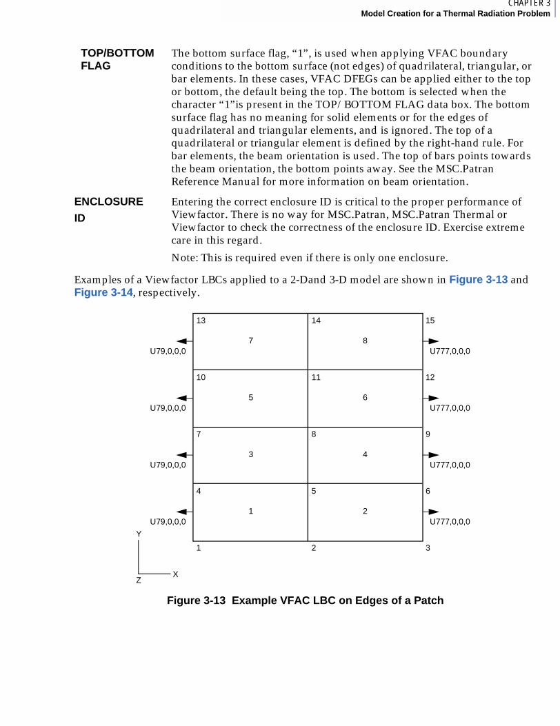
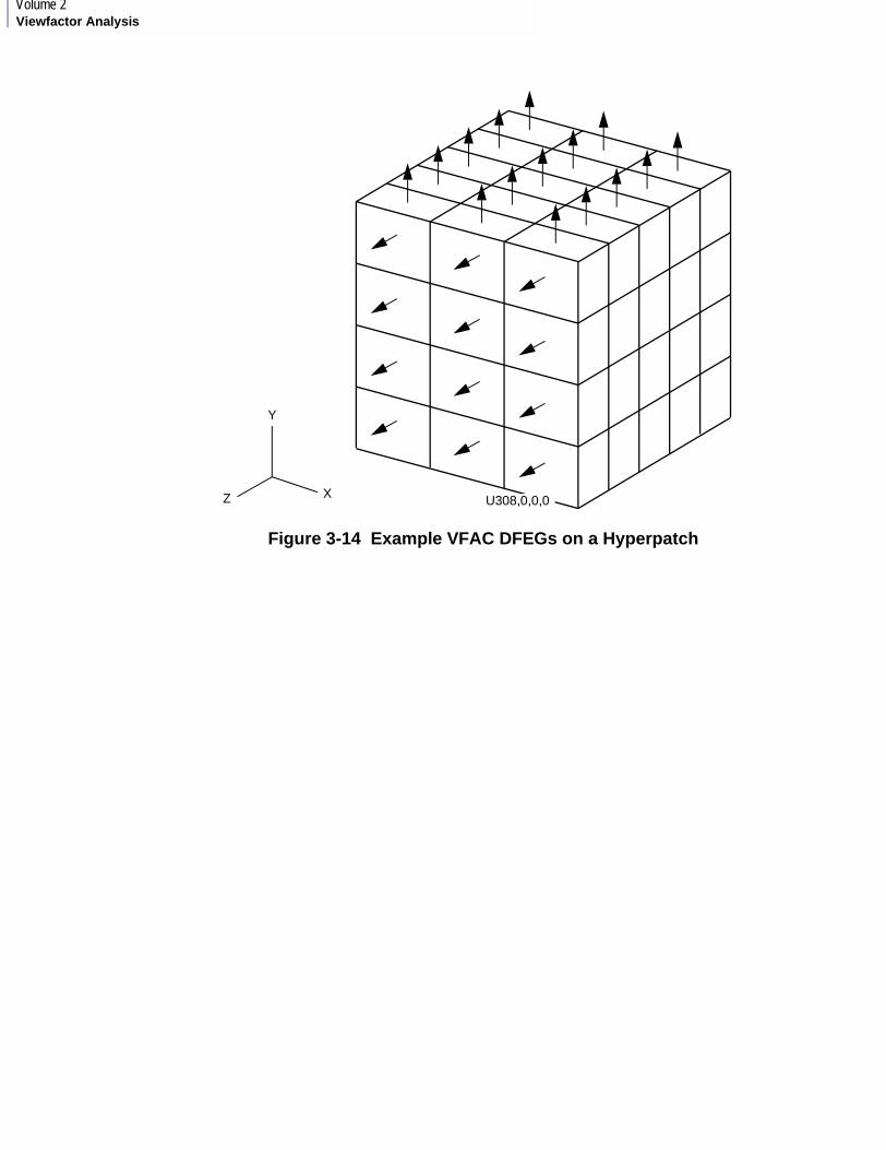
Examples of a Viewfactor LBCs applied to a 2-Dand 3-D model are shown in Figure 3-13 and Figure 3-14, respectively.
Figure 3-13 Example VFAC LBC on Edges of a Patch
TOP/BOTTOMFLAG
The bottom surface flag, “1”, is used when applying VFAC boundary conditions to the bottom surface (not edges) of quadrilateral, triangular, or bar elements. In these cases, VFAC DFEGs can be applied either to the top or bottom, the default being the top. The bottom is selected when the character “1”is present in the TOP/BOTTOM FLAG data box. The bottom surface flag has no meaning for solid elements or for the edges of quadrilateral and triangular elements, and is ignored. The top of a quadrilateral or triangular element is defined by the right-hand rule. For bar elements, the beam orientation is used. The top of bars points towards the beam orientation, the bottom points away. See the MSC.Patran Reference Manual for more information on beam orientation.
ENCLOSURE
ID
Entering the correct enclosure ID is critical to the proper performance of Viewfactor. There is no way for MSC.Patran, MSC.Patran Thermal or Viewfactor to check the correctness of the enclosure ID. Exercise extreme care in this regard.
Note: This is required even if there is only one enclosure.
U79,0,0,0
U79,0,0,0
U79,0,0,0
U79,0,0,0
U777,0,0,0
U777,0,0,0
U777,0,0,0
U777,0,0,0
15
12
9
6
3
14
11
8
5
2
13
10
7
4
1
7
5
3
1
8
6
4
2
Y
ZX
Volume 2Viewfactor Analysis
Figure 3-14 Example VFAC DFEGs on a Hyperpatch
Y
XZ U308,0,0,0
4CHAPTER 3Model Creation for a Thermal Radiation Problem
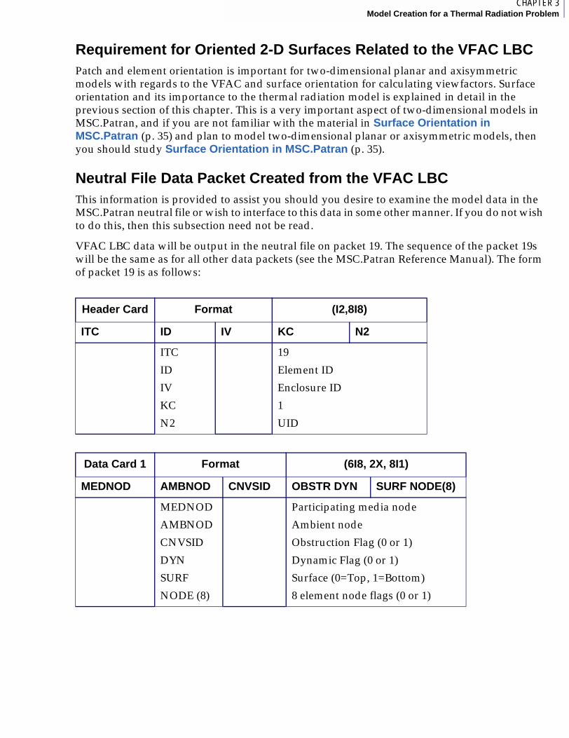
Requirement for Oriented 2-D Surfaces Related to the VFAC LBCPatch and element orientation is important for two-dimensional planar and axisymmetric models with regards to the VFAC and surface orientation for calculating viewfactors. Surface orientation and its importance to the thermal radiation model is explained in detail in the previous section of this chapter. This is a very important aspect of two-dimensional models in MSC.Patran, and if you are not familiar with the material in Surface Orientation in MSC.Patran (p. 35) and plan to model two-dimensional planar or axisymmetric models, then you should study Surface Orientation in MSC.Patran (p. 35).
Neutral File Data Packet Created from the VFAC LBCThis information is provided to assist you should you desire to examine the model data in the MSC.Patran neutral file or wish to interface to this data in some other manner. If you do not wish to do this, then this subsection need not be read.
VFAC LBC data will be output in the neutral file on packet 19. The sequence of the packet 19s will be the same as for all other data packets (see the MSC.Patran Reference Manual). The form of packet 19 is as follows:
Header Card Format (I2,8I8)
ITC ID IV KC N2
ITC
ID
IV
KC
N2
19
Element ID
Enclosure ID
1
UID
Data Card 1 Format (6I8, 2X, 8I1)
MEDNOD AMBNOD CNVSID OBSTR DYN SURF NODE(8)
MEDNOD
AMBNOD
CNVSID
DYN
SURF
NODE (8)
Participating media node
Ambient node
Obstruction Flag (0 or 1)
Dynamic Flag (0 or 1)
Surface (0=Top, 1=Bottom)
8 element node flags (0 or 1)

Volume 2Viewfactor Analysis
3.5 Advanced Features of the VFAC Boundary ConditionThe Viewfactor boundary condition in MSC.Patran was designed to support modeling a media participating in the thermal radiation interchange. This interchange could take place between two surfaces or between a surface and an ambient or space node representing the background thermal radiation conditions. The participating medium is assumed to be isothermal and gray within each waveband and to be diffusely emitting and absorbing without photoactive effects.
The VFAC boundary condition also provides support for some capabilities in Viewfactor which are used to reduce the CPU time required to calculate the viewfactors. This support comes in the form of the CNVSID and nonobstruction FLAG parameters in the VFAC LBC form which are used to identify convex surfaces and nonobstructing surfaces, respectively, in MSC.Patran.
These features of the VFAC boundary condition are described in this section.
Referencing Participating Media Radiation NodesThe participating medium is assumed to be at a uniform temperature, gray in a waveband, and diffuse. It is assumed to be weakly absorbing (i.e., the exact exponential absorption function may be accurately replaced with a linear approximation). It is assumed that the medium does not obscure itself or the other surfaces.
Role of Radiation Participating Media in MSC.Patran Thermal. The MSC.Patran Thermal user is free to assign the temperature or heat flux to the participating media node as a simple constant or in more complicated situations as functions of time and temperatures of other nodes. The participating media node will be treated as any other node in the thermal resistor network.
Participating Media Resistor Networks. When the participating media node is present, the Viewfactor code makes three resistors instead of the usual one resistor between the surface subareas. One of the resistors will still be between the surface subareas. But it will have been modified to account for the portion of the radiant energy which will be absorbed as it traverses between the two surfaces. The second and third resistors will be between the surface subareas for each surface and the participating media node. They will account for the radiant interchange between the surfaces and the participating media. Refer to the MSC.Patran Thermal User’s Guide for an explanation of resistor networks and subareas. Two resistor networks are shown in Figure 3-15, one without a participating medium and one with a medium.
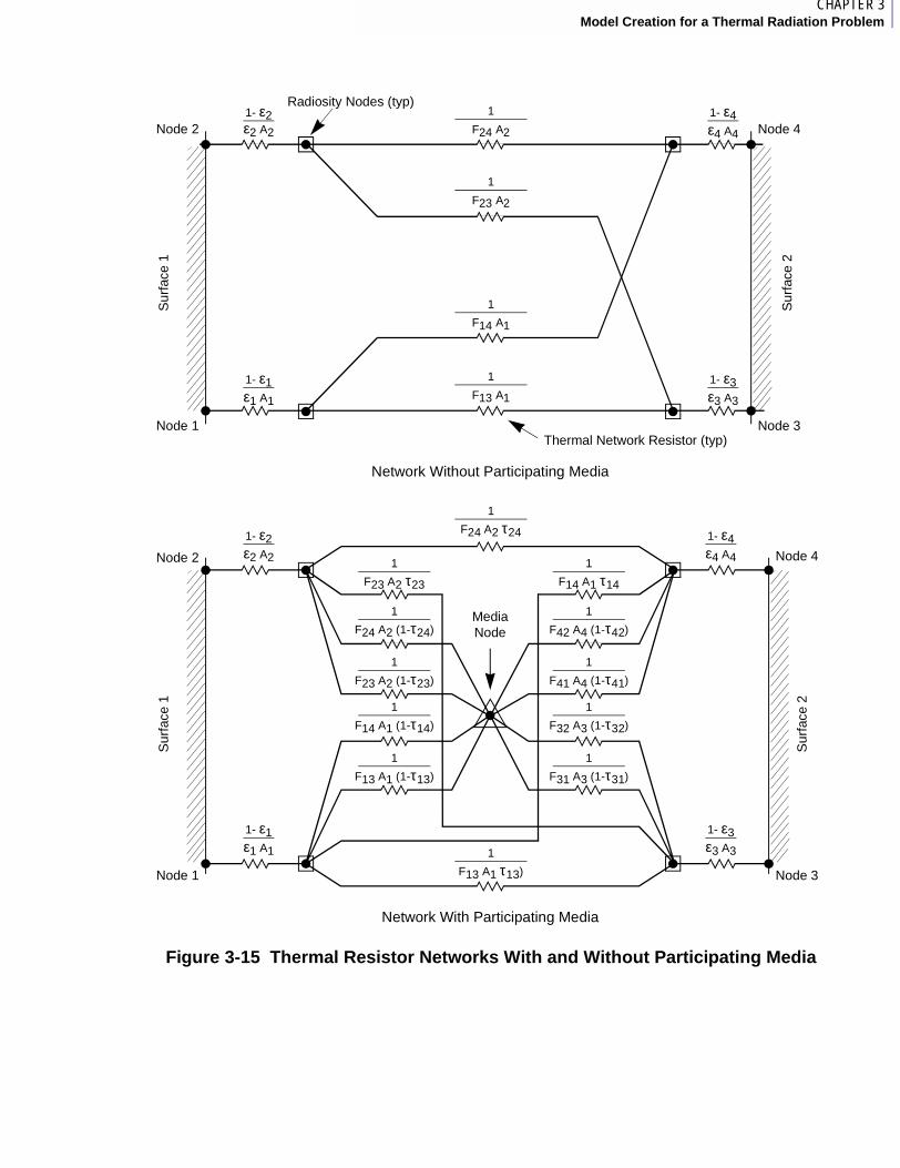
4CHAPTER 3Model Creation for a Thermal Radiation Problem
Figure 3-15 Thermal Resistor Networks With and Without Participating Media
Node 2
Node 1
Node 2 Node 4
Node 1 Node 3
Sur
face
1S
urfa
ce 1
Sur
face
2
Radiosity Nodes (typ)
Thermal Network Resistor (typ)
Network Without Participating Media
Network With Participating Media
1
F31 A3 (1-τ31)
1
F32 A3 (1-τ32)
1
F41 A4 (1-τ41)
1
F42 A4 (1-τ42)
1
F14 A1 τ14
1
F13 A1 (1-τ13)
1
F14 A1 (1-τ14)
1
F23 A2 (1-τ23)
1
F24 A2 (1-τ24)
1
F23 A2 τ23
1
F24 A2 τ24
1
F13 A1 τ13)
1- ε4ε4 A4
1- ε3ε3 A3
1- ε2ε2 A2
1- ε1ε1 A1
1- ε1ε1 A1
1- ε4ε4 A4
1- ε3ε3 A3
1
F13 A1
1
F14 A1
1
F23 A2
1
F24 A2
MediaNode
Node 4
Node 3
Sur
face
2
1- ε2ε2 A2

Volume 2Viewfactor Analysis
Defining the Participating Media Node. The participating media node must be defined in the MSC.Patran model before it can be referenced in the VFAC LBC form. If the participating media node does not already exist, it may be created with the MSC.Patran Finite Element form:
In the node location list box, point to a convenient grid point.
Finite Element
Action: Create
Object: Node
Method: Edit
Note: The exact location of this node is not important. For clarity, you may want to use a conspicuous node ID number such as 1000, 9999.

5CHAPTER 3Model Creation for a Thermal Radiation Problem
Referencing Ambient or Space Radiation NodesFrequently in thermal radiation analysis we encounter a problem which has an enclosure with an opening to space or to the ambient environment. In order to facilitate modeling this situation, Viewfactor and MSC.Patran Thermal provide for ambient thermal radiation nodes. The MSC.Patran Viewfactor boundary condition provides support for entering this part of the model through the MSC.Patran preprocessing.
Role of Ambient Radiation Nodes. In the present analysis scheme for a given enclosure, each surface may see at most one ambient node. This implies that each surface in the enclosure sees an isothermal ambient environment. If there is a participating media present, it is assumed to exchange radiant energy with the ambient environment also. The distance from the ambient node to the participating media node is not well defined. Therefore, this combination cannot be used with MSC.Patran Thermal resistor types which calculate the media absorption and emittance from Beer’s Law of Absorption (i.e., resistor subtypes 7, 8, 11, and 12).
Suggested Practices to Improve Model Accuracy. There is a way to produce a more accurate model of the thermal radiation interchange between a surface and the ambient radiation through an opening in the enclosure. This is done by covering the openings in the enclosure with surfaces having the temperature of the ambient environment. The viewfactor from the surface to the ambient environment is calculated by taking one minus the sum of the viewfactors to all other surfaces that the first surface can see. This summing process introduces the possibility of cumulative errors. By filling the enclosure openings with ambient surfaces, the error is only the error occurring in the viewfactor calculation from the first surface to the ambient surface.
This method does in general require more CPU time, but this increase in CPU time will be relatively small if the ambient surfaces needed to close the open enclosure are few compared to the total number of surfaces in the enclosure. This method also has another advantage. There are no restrictions on the use of MSC.Patran Thermal radiation resistors which use Beer’s Law to calculate the interaction with the participating media (see Role of Ambient Radiation Nodes). This method allows you to have nonuniform ambient temperatures and to model the radiative surface properties of the ambient environment.
Some examples of open enclosures and how they might be closed by ambient surfaces are shown in Figure 3-16.
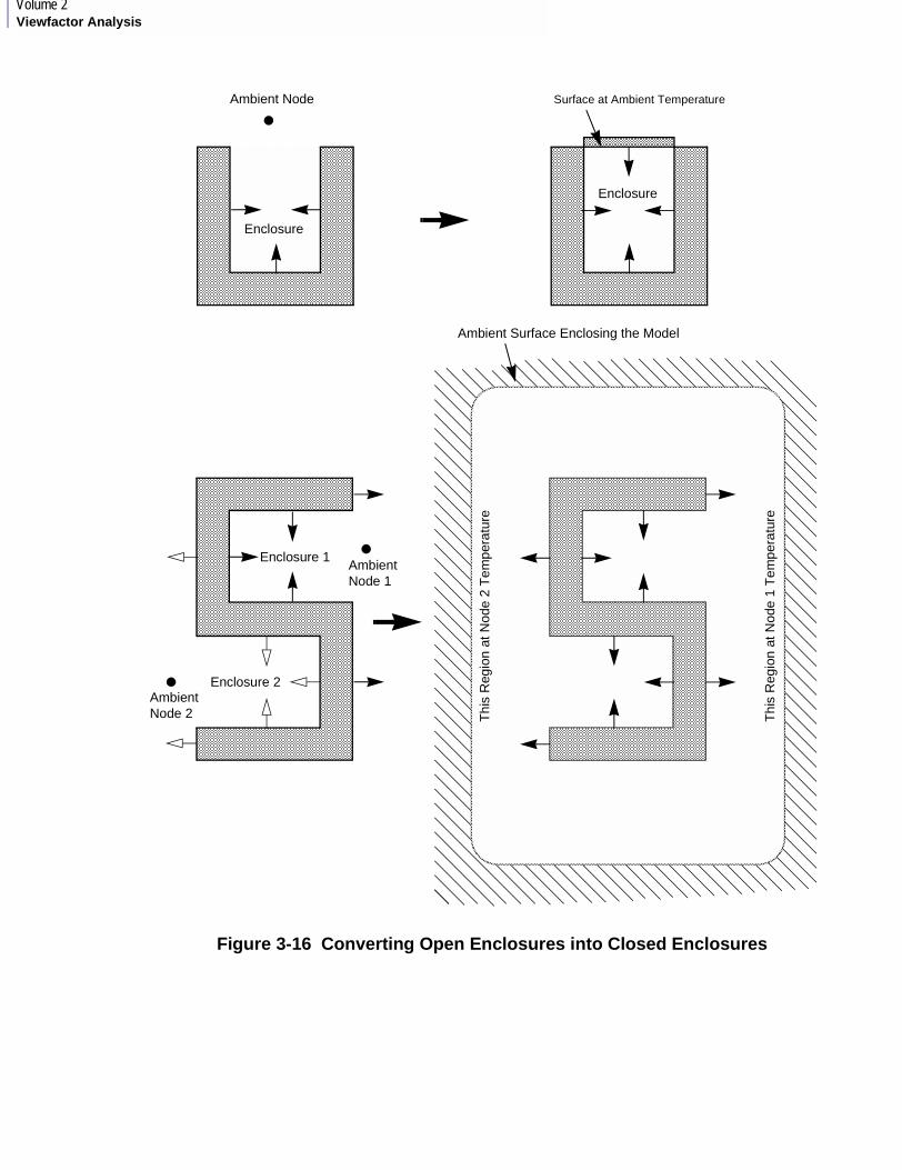
Volume 2Viewfactor Analysis
Figure 3-16 Converting Open Enclosures into Closed Enclosures
Enclosure
Enclosure
Ambient Node Surface at Ambient Temperature
Enclosure 1 AmbientNode 1
Enclosure 2 AmbientNode 2 T
his
Reg
ion
at N
ode
2 T
empe
ratu
re
Thi
s R
egio
n at
Nod
e 1
Tem
pera
ture
Ambient Surface Enclosing the Model
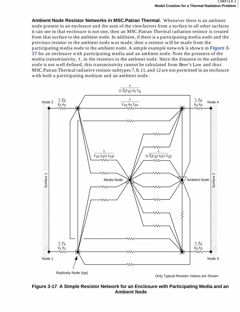
5CHAPTER 3Model Creation for a Thermal Radiation Problem
Ambient Node Resistor Networks in MSC.Patran Thermal. Whenever there is an ambient node present in an enclosure and the sum of the viewfactors from a surface to all other surfaces it can see in that enclosure is not one, then an MSC.Patran Thermal radiation resistor is created from that surface to the ambient node. In addition, if there is a participating media node and the previous resistor to the ambient node was made, then a resistor will be made from the participating media node to the ambient node. A simple example network is shown in Figure 3-17 for an enclosure with participating media and an ambient node. Note the presence of the media transmissivity, , in the resistors to the ambient node. Since the distance to the ambient node is not well defined, this transmissivity cannot be calculated from Beer’s Law and thus MSC.Patran Thermal radiative resistor subtypes 7, 8, 11, and 12 are not permitted in an enclosure with both a participating medium and an ambient node.
Figure 3-17 A Simple Resistor Network for an Enclosure with Participating Media and an Ambient Node
τ
Node 21- ε4ε4 A4
1
F24 A4 τ24
Media Node Ambient Node
1- ε3ε3 A3
1- ε2ε2 A2
1- ε1ε1 A1
Node 4
Node 1 Node 3
Radiosity Node (typ)Only Typical Resistor Values are Shown
1
(1-ΣjF2j) A2 τ2j
1
(1-ΣjF2j) A2(1-τ2j)
1
F24 A2(1-τ24)
Sur
face
2
Sur
face
1
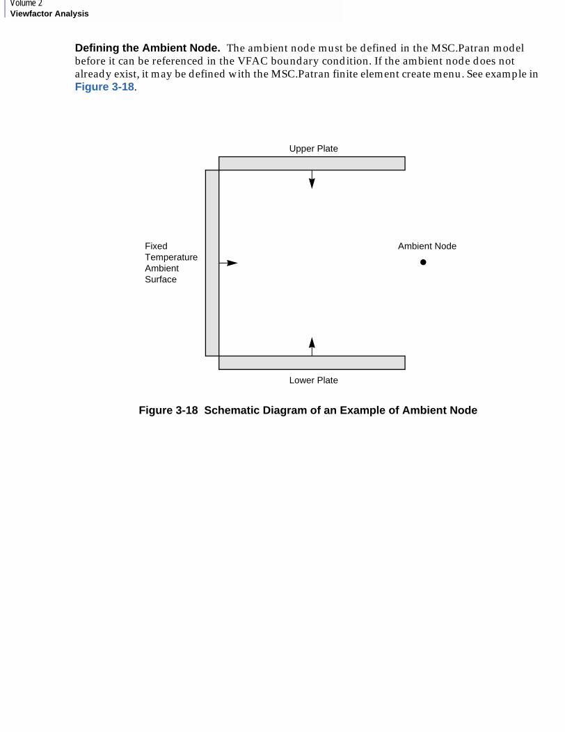
Volume 2Viewfactor Analysis
Defining the Ambient Node. The ambient node must be defined in the MSC.Patran model before it can be referenced in the VFAC boundary condition. If the ambient node does not already exist, it may be defined with the MSC.Patran finite element create menu. See example in Figure 3-18.
Figure 3-18 Schematic Diagram of an Example of Ambient Node
FixedTemperatureAmbientSurface
Lower Plate
Ambient Node
Upper Plate
5CHAPTER 3Model Creation for a Thermal Radiation Problem
Identifying a Surface as Being ConvexSince the calculation of viewfactors is computationally expensive, we have provided the user with the ability to identify convex surfaces in the thermal radiation portion of the model. A convex surface is one for which no pair of points on the surface can see each other by direct line of sight. Thus the exterior of a sphere and the exterior of a cylinder are convex surfaces. Plane surfaces are also considered to be convex. Thus, for example, the faces of a cube are all convex, and the entire exterior of a cube is convex, while the interior of the cube has six separate convex surfaces, one for each face. Caution must be exercised when specifying convex surfaces in axisymmetric models (see Caveats Regarding Convex Surfaces in Axisymmetric Models (p. 55).
Significance of Convex Surfaces to Viewfactor Calculations. To calculate viewfactors, each surface must be paired with every other surface in the enclosure and a determination made regarding whether there is a direct line of sight view between pairs of points on these two surfaces, one point on each surface. By the nature of convex surfaces, we know a priori that a pair of surfaces, element faces in our case, on a convex surface do not have a direct line of sight view of each other.
Benefits of Identifying Convex Surfaces to Viewfactor Execution Time. This determination of whether one surface has a line of sight view of another surface from geometrical considerations is computationally significant. If the determination can be made simply by comparing convex surface IDs (a computationally trivial test) a significant amount of CPU time can be saved on problems which have a large number of element faces on convex surfaces in an enclosure.
This requires that the convex surfaces be identified by the user before they are submitted to Viewfactor for analysis. This of course is not required in order to run Viewfactor. You will have to decide whether it is an economical use of your time to identify convex surfaces in order to save some computational time. People seem to be more efficient than machines at identifying convex surfaces and are able to group large numbers of element faces into convex surfaces merely by looking briefly at the model.
Caveats Regarding Convex Surfaces in Axisymmetric Models. In certain situations, you must take special care not to identify as convex surfaces which are not really convex. A simple example of this is the exterior of a torus, which appears convex when the axisymmetric model is drawn, but in reality, due to its double curvature, is partially not convex. This example is illustrated in Figure 3-20. Such situations are common in axisymmetric models and also can
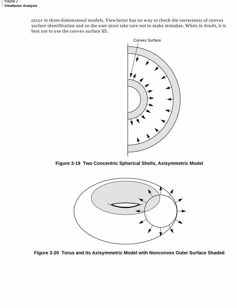
Volume 2Viewfactor Analysis
occur in three-dimensional models. Viewfactor has no way to check the correctness of convex surface identification and so the user must take care not to make mistakes. When in doubt, it is best not to use the convex surface ID.
Figure 3-19 Two Concentric Spherical Shells, Axisymmetric Model
Figure 3-20 Torus and its Axisymmetric Model with Nonconvex Outer Surface Shaded
Convex Surface
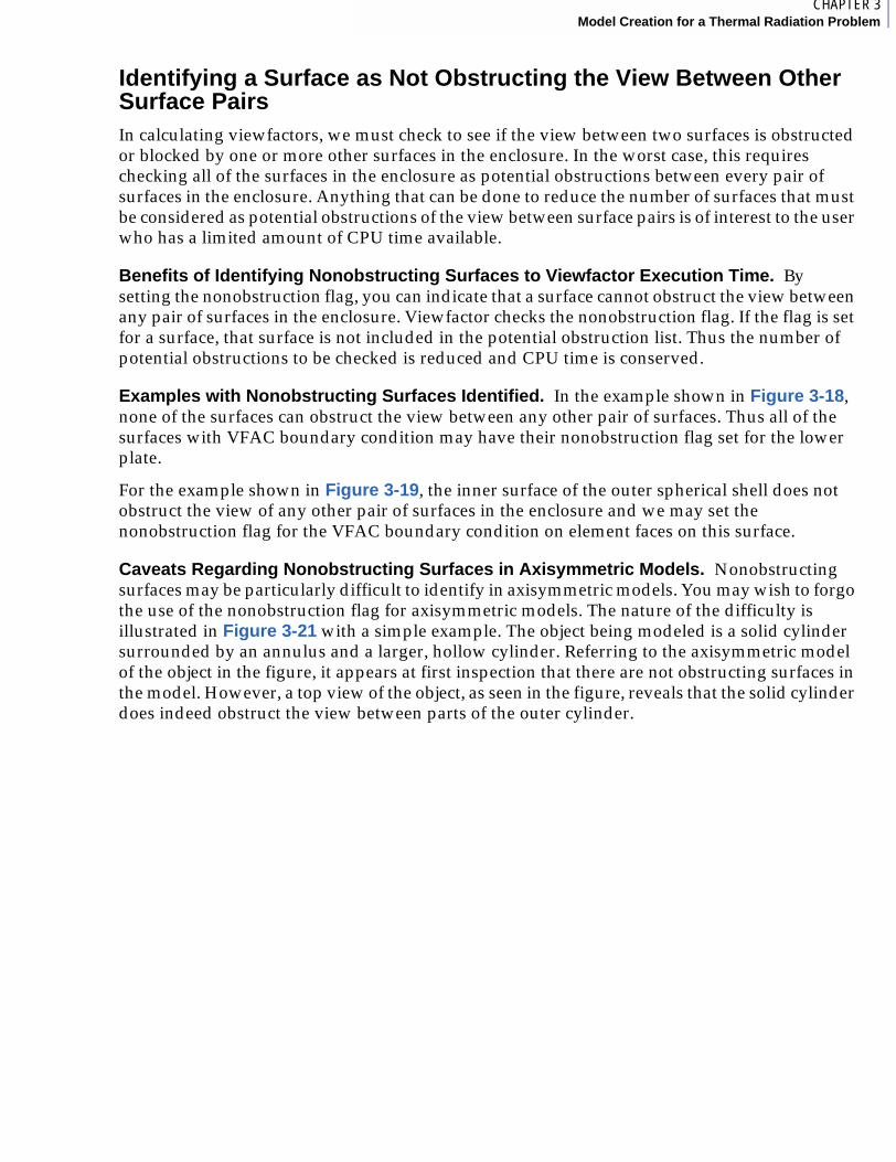
5CHAPTER 3Model Creation for a Thermal Radiation Problem
Identifying a Surface as Not Obstructing the View Between Other Surface PairsIn calculating viewfactors, we must check to see if the view between two surfaces is obstructed or blocked by one or more other surfaces in the enclosure. In the worst case, this requires checking all of the surfaces in the enclosure as potential obstructions between every pair of surfaces in the enclosure. Anything that can be done to reduce the number of surfaces that must be considered as potential obstructions of the view between surface pairs is of interest to the user who has a limited amount of CPU time available.
Benefits of Identifying Nonobstructing Surfaces to Viewfactor Execution Time. By setting the nonobstruction flag, you can indicate that a surface cannot obstruct the view between any pair of surfaces in the enclosure. Viewfactor checks the nonobstruction flag. If the flag is set for a surface, that surface is not included in the potential obstruction list. Thus the number of potential obstructions to be checked is reduced and CPU time is conserved.
Examples with Nonobstructing Surfaces Identified. In the example shown in Figure 3-18, none of the surfaces can obstruct the view between any other pair of surfaces. Thus all of the surfaces with VFAC boundary condition may have their nonobstruction flag set for the lower plate.
For the example shown in Figure 3-19, the inner surface of the outer spherical shell does not obstruct the view of any other pair of surfaces in the enclosure and we may set the nonobstruction flag for the VFAC boundary condition on element faces on this surface.
Caveats Regarding Nonobstructing Surfaces in Axisymmetric Models. Nonobstructing surfaces may be particularly difficult to identify in axisymmetric models. You may wish to forgo the use of the nonobstruction flag for axisymmetric models. The nature of the difficulty is illustrated in Figure 3-21 with a simple example. The object being modeled is a solid cylinder surrounded by an annulus and a larger, hollow cylinder. Referring to the axisymmetric model of the object in the figure, it appears at first inspection that there are not obstructing surfaces in the model. However, a top view of the object, as seen in the figure, reveals that the solid cylinder does indeed obstruct the view between parts of the outer cylinder.
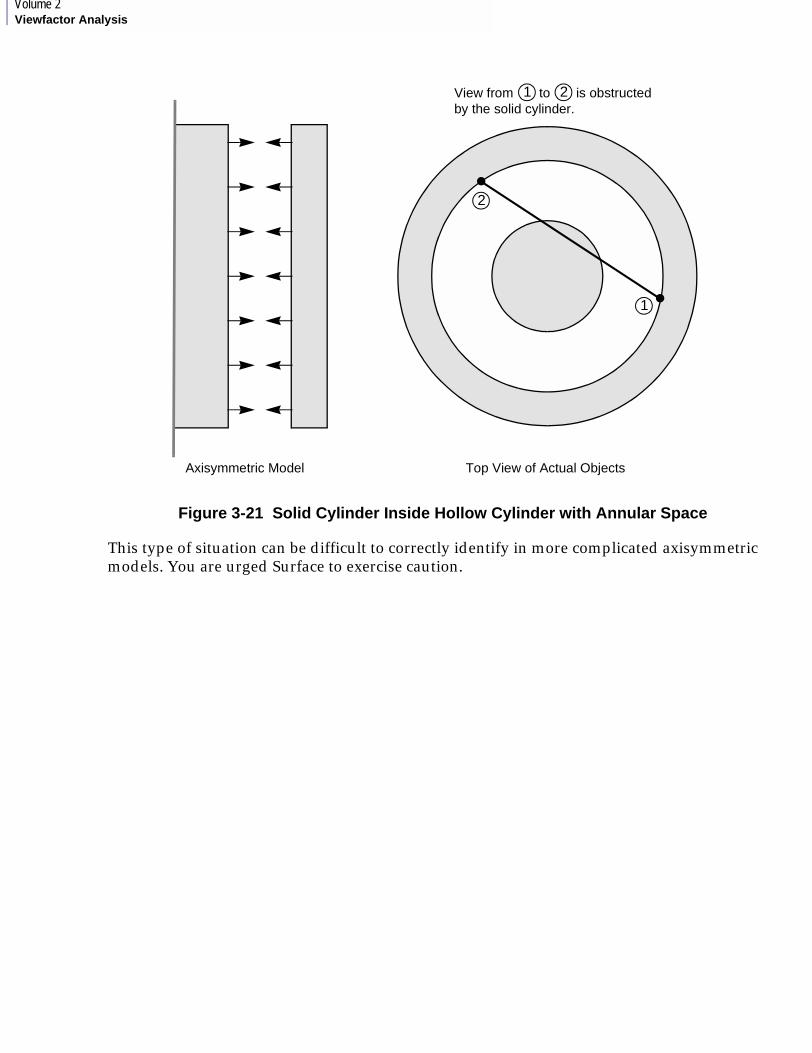
Volume 2Viewfactor Analysis
Figure 3-21 Solid Cylinder Inside Hollow Cylinder with Annular Space
This type of situation can be difficult to correctly identify in more complicated axisymmetric models. You are urged Surface to exercise caution.
View from to is obstructedby the solid cylinder.
1 2
1
2
Top View of Actual Objects Axisymmetric Model
5CHAPTER 3Model Creation for a Thermal Radiation Problem
3.6 Relationship of VFAC LBC Data to VFINDAT File DataThe Viewfactor boundary condition data is output from MSC.Patran in the neutral file packet 19s. The neutral file is read by MSC.Patran Thermal’s PATQ and translated into the Viewfactor input file VFINDAT. The VFINDAT file is described in detail in Chapter 9. The relationship of data in the neutral file to data in the VFINDAT file is described in general terms.
The VFINDAT file begins with title data for the problem, followed by data about the size of the problem. Next is symmetry data which is discussed in Compatibility Requirements for Model and VFAC Templates (p. 76). All of the nodes in the MSC.Patran model are then copied to the VFINDAT file, including their IDs and coordinates.
The surfaces with VFAC boundary conditions are then grouped into their respective enclosures and put out to the VFINDAT file grouped by enclosure. Some of the data in the VFAC record is copied directly. This data is the enclosure ID, the user function ID or TID, the participating media node or MEDNOD, the ambient node or AMBNOD, and the convex surface ID or CNVSID. The nonobstruction flag is translated to 0 or 1 and copied. The element ID with which each surface is associated is in the packet 19 and also copied to VFINDAT.
The VFINDAT file also requires other information about the surface. This is developed by PATQ from data about the model from other parts of the neutral file. This data includes information about the shape of the surface, the order of interpolation functions needed to describe the surface, the number of nodes associated with the surface, an ID for the surface, an identification of the element face represented by this surface, the node IDs associated with this surface, and possibly some other data associated with the surface.
Volume 2Viewfactor Analysis
3.7 MSC.Patran Thermal TEMPLATEDAT Files for Surface Property DescriptionMSC.Patran Thermal supports an arbitrary finite number of wavebands for spectral dependent material properties for thermal radiation interchange. Within each waveband the material properties are assumed to be independent of wavelength (gray) and diffuse. Completely gray surfaces are also supported without the added work on your part to specify the waveband as the entire spectrum. This section describes the data needed by Viewfactor in the form of the MSC.Patran Thermal TEMPLATEDAT file and VFAC template to make the MSC.Patran Thermal thermal network resistors for modeling thermal radiation interchange.
Thermal Radiation Wavebands as Used in MSC.Patran Thermal User’s GuideIf you only plan to use gray surfaces, then the information on thermal radiation wavebands and wavelength dependent network resistors may be ignored. If the wavelength dependence is not specified by entering the wavebands, then Viewfactor assumes that the enclosure is gray and you need not be concerned with wavebands.
Thermal radiation wavebands are defined in the Viewfactor code for use by P⁄ THERMAL in terms of their beginning and ending wavelengths in units of microns. The spectrum begins at zero wavelength and extends to infinity. Since infinity is not a convenient quantity with which to work in computers, we will use some finite, but large number to represent the upper end of the spectrum, for example 1.0E10 microns. In general, the thermal radiation above this wavelength is completely negligible for engineering problems. (This may not be true in certain physics problems.)
MSC.Patran Thermal evaluates the black body function in each waveband and at the temperature of each surface. This is an improvement over other methods which use some mean temperature between the surface pairs (e.g., geometric mean, for the black body temperature). The heat flow between two surfaces 1 and 2 as represented by the MSC.Patran Thermal network equations is
Eq. 3-1
where:
i= Waveband index
s= Stefan-Boltsmann constant
nbands= Number of wavebands
F= Black body function from at temperature T
T1,T2= Temperatures of surfaces 1 and 2, respectively
R= Effective radiative resistance between surfaces 1 and 2, taking into account possibly time, temperature, and waveband
t= Time
l= Wave length
Q t( )1 2⇒
σ F λ( i 1– λ i, T1 t( ) t )T 14 t( ), F λ i 1– λ i T, 2 t( ) t )T 2
4 t( ), ,–,
R λ i 1– λ i T1 t( ) T2 t( ) t,,, ,( )----------------------------------------------------------------------------------------------------------------------------------------------------------------------------
i 1=
nbands∑=
λ i 1– to λ i
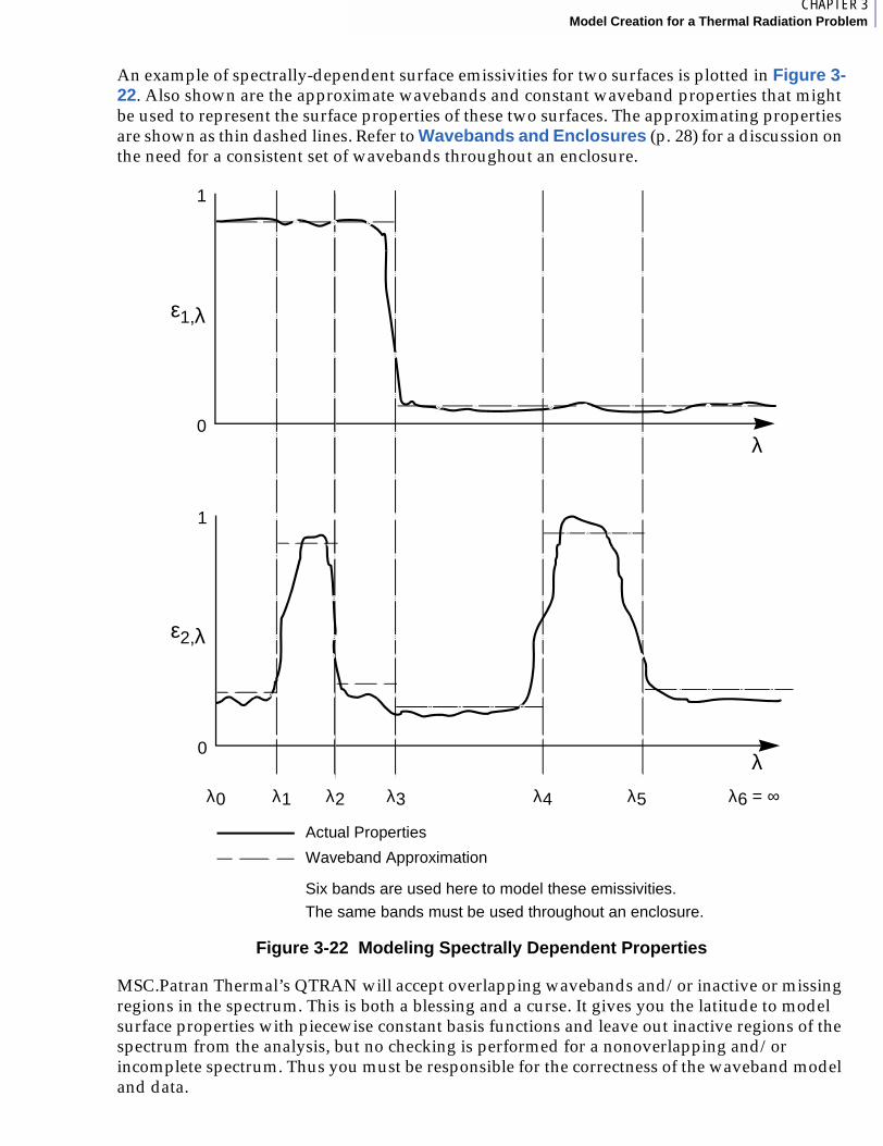
6CHAPTER 3Model Creation for a Thermal Radiation Problem
An example of spectrally-dependent surface emissivities for two surfaces is plotted in Figure 3-22. Also shown are the approximate wavebands and constant waveband properties that might be used to represent the surface properties of these two surfaces. The approximating properties are shown as thin dashed lines. Refer to Wavebands and Enclosures (p. 28) for a discussion on the need for a consistent set of wavebands throughout an enclosure.
Figure 3-22 Modeling Spectrally Dependent Properties
MSC.Patran Thermal’s QTRAN will accept overlapping wavebands and/or inactive or missing regions in the spectrum. This is both a blessing and a curse. It gives you the latitude to model surface properties with piecewise constant basis functions and leave out inactive regions of the spectrum from the analysis, but no checking is performed for a nonoverlapping and/or incomplete spectrum. Thus you must be responsible for the correctness of the waveband model and data.
λ0
1
ε1,λ
ε2,λ
λ0 λ1 λ2 λ3 λ4 λ5 λ6 = ∞
0
1
Actual Properties
Six bands are used here to model these emissivities.
The same bands must be used throughout an enclosure.
Waveband Approximation
λ
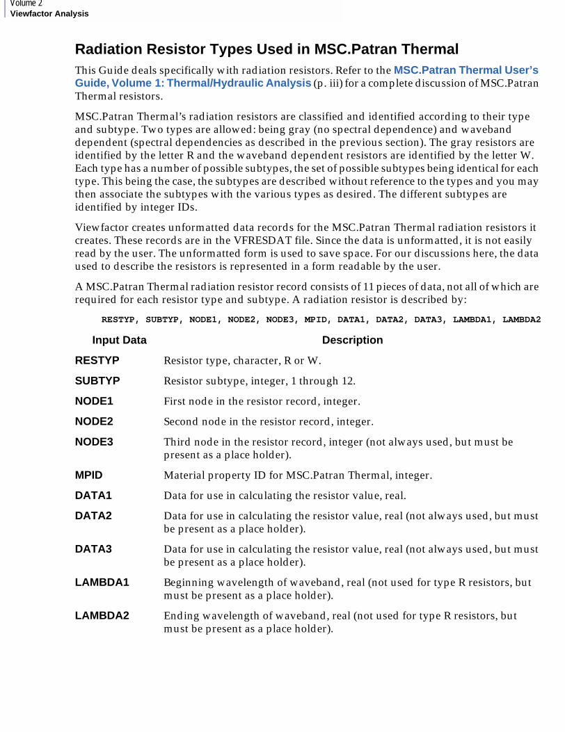
Volume 2Viewfactor Analysis
Radiation Resistor Types Used in MSC.Patran ThermalThis Guide deals specifically with radiation resistors. Refer to the MSC.Patran Thermal User’s Guide, Volume 1: Thermal/Hydraulic Analysis (p. iii) for a complete discussion of MSC.Patran Thermal resistors.
MSC.Patran Thermal’s radiation resistors are classified and identified according to their type and subtype. Two types are allowed: being gray (no spectral dependence) and waveband dependent (spectral dependencies as described in the previous section). The gray resistors are identified by the letter R and the waveband dependent resistors are identified by the letter W. Each type has a number of possible subtypes, the set of possible subtypes being identical for each type. This being the case, the subtypes are described without reference to the types and you may then associate the subtypes with the various types as desired. The different subtypes are identified by integer IDs.
Viewfactor creates unformatted data records for the MSC.Patran Thermal radiation resistors it creates. These records are in the VFRESDAT file. Since the data is unformatted, it is not easily read by the user. The unformatted form is used to save space. For our discussions here, the data used to describe the resistors is represented in a form readable by the user.
A MSC.Patran Thermal radiation resistor record consists of 11 pieces of data, not all of which are required for each resistor type and subtype. A radiation resistor is described by:
RESTYP, SUBTYP, NODE1, NODE2, NODE3, MPID, DATA1, DATA2, DATA3, LAMBDA1, LAMBDA2
Input Data Description
RESTYP Resistor type, character, R or W.
SUBTYP Resistor subtype, integer, 1 through 12.
NODE1 First node in the resistor record, integer.
NODE2 Second node in the resistor record, integer.
NODE3 Third node in the resistor record, integer (not always used, but must be present as a place holder).
MPID Material property ID for MSC.Patran Thermal, integer.
DATA1 Data for use in calculating the resistor value, real.
DATA2 Data for use in calculating the resistor value, real (not always used, but must be present as a place holder).
DATA3 Data for use in calculating the resistor value, real (not always used, but must be present as a place holder).
LAMBDA1 Beginning wavelength of waveband, real (not used for type R resistors, but must be present as a place holder).
LAMBDA2 Ending wavelength of waveband, real (not used for type R resistors, but must be present as a place holder).
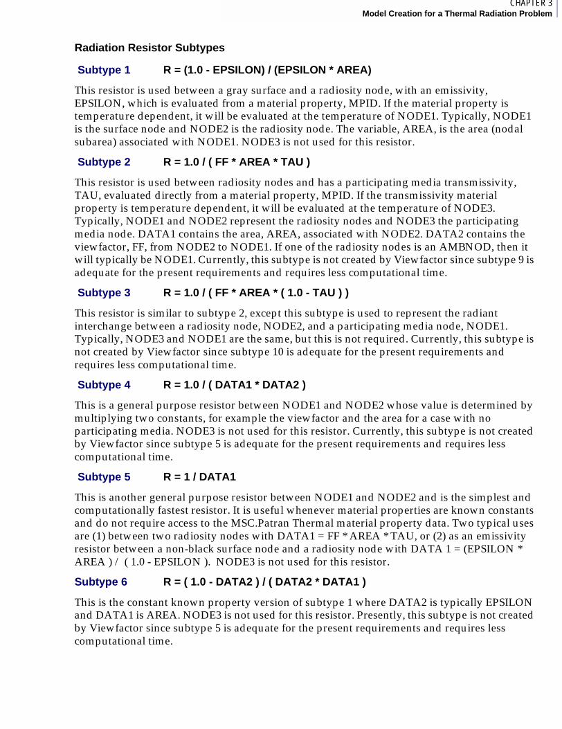
6CHAPTER 3Model Creation for a Thermal Radiation Problem
Radiation Resistor Subtypes
Subtype 1 R = (1.0 - EPSILON) / (EPSILON * AREA)
This resistor is used between a gray surface and a radiosity node, with an emissivity, EPSILON, which is evaluated from a material property, MPID. If the material property is temperature dependent, it will be evaluated at the temperature of NODE1. Typically, NODE1 is the surface node and NODE2 is the radiosity node. The variable, AREA, is the area (nodal subarea) associated with NODE1. NODE3 is not used for this resistor.
Subtype 2 R = 1.0 / ( FF * AREA * TAU )
This resistor is used between radiosity nodes and has a participating media transmissivity, TAU, evaluated directly from a material property, MPID. If the transmissivity material property is temperature dependent, it will be evaluated at the temperature of NODE3. Typically, NODE1 and NODE2 represent the radiosity nodes and NODE3 the participating media node. DATA1 contains the area, AREA, associated with NODE2. DATA2 contains the viewfactor, FF, from NODE2 to NODE1. If one of the radiosity nodes is an AMBNOD, then it will typically be NODE1. Currently, this subtype is not created by Viewfactor since subtype 9 is adequate for the present requirements and requires less computational time.
Subtype 3 R = 1.0 / ( FF * AREA * ( 1.0 - TAU ) )
This resistor is similar to subtype 2, except this subtype is used to represent the radiant interchange between a radiosity node, NODE2, and a participating media node, NODE1. Typically, NODE3 and NODE1 are the same, but this is not required. Currently, this subtype is not created by Viewfactor since subtype 10 is adequate for the present requirements and requires less computational time.
Subtype 4 R = 1.0 / ( DATA1 * DATA2 )
This is a general purpose resistor between NODE1 and NODE2 whose value is determined by multiplying two constants, for example the viewfactor and the area for a case with no participating media. NODE3 is not used for this resistor. Currently, this subtype is not created by Viewfactor since subtype 5 is adequate for the present requirements and requires less computational time.
Subtype 5 R = 1 / DATA1
This is another general purpose resistor between NODE1 and NODE2 and is the simplest and computationally fastest resistor. It is useful whenever material properties are known constants and do not require access to the MSC.Patran Thermal material property data. Two typical uses are (1) between two radiosity nodes with DATA1 = FF * AREA * TAU, or (2) as an emissivity resistor between a non-black surface node and a radiosity node with DATA 1 = (EPSILON * AREA ) / ( 1.0 - EPSILON ). NODE3 is not used for this resistor.
Subtype 6 R = ( 1.0 - DATA2 ) / ( DATA2 * DATA1 )
This is the constant known property version of subtype 1 where DATA2 is typically EPSILON and DATA1 is AREA. NODE3 is not used for this resistor. Presently, this subtype is not created by Viewfactor since subtype 5 is adequate for the present requirements and requires less computational time.
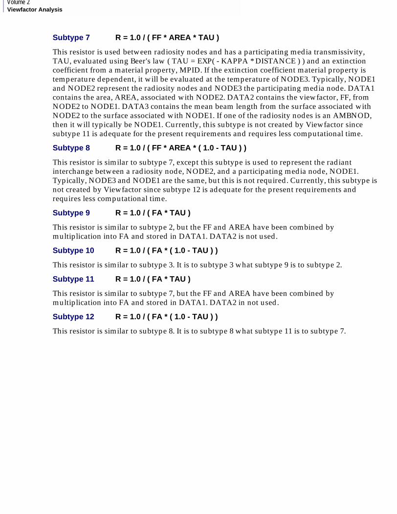
Volume 2Viewfactor Analysis
Subtype 7 R = 1.0 / ( FF * AREA * TAU )
This resistor is used between radiosity nodes and has a participating media transmissivity, TAU, evaluated using Beer's law ( TAU = EXP( - KAPPA * DISTANCE ) ) and an extinction coefficient from a material property, MPID. If the extinction coefficient material property is temperature dependent, it will be evaluated at the temperature of NODE3. Typically, NODE1 and NODE2 represent the radiosity nodes and NODE3 the participating media node. DATA1 contains the area, AREA, associated with NODE2. DATA2 contains the viewfactor, FF, from NODE2 to NODE1. DATA3 contains the mean beam length from the surface associated with NODE2 to the surface associated with NODE1. If one of the radiosity nodes is an AMBNOD, then it will typically be NODE1. Currently, this subtype is not created by Viewfactor since subtype 11 is adequate for the present requirements and requires less computational time.
Subtype 8 R = 1.0 / ( FF * AREA * ( 1.0 - TAU ) )
This resistor is similar to subtype 7, except this subtype is used to represent the radiant interchange between a radiosity node, NODE2, and a participating media node, NODE1. Typically, NODE3 and NODE1 are the same, but this is not required. Currently, this subtype is not created by Viewfactor since subtype 12 is adequate for the present requirements and requires less computational time.
Subtype 9 R = 1.0 / ( FA * TAU )
This resistor is similar to subtype 2, but the FF and AREA have been combined by multiplication into FA and stored in DATA1. DATA2 is not used.
Subtype 10 R = 1.0 / ( FA * ( 1.0 - TAU ) )
This resistor is similar to subtype 3. It is to subtype 3 what subtype 9 is to subtype 2.
Subtype 11 R = 1.0 / ( FA * TAU )
This resistor is similar to subtype 7, but the FF and AREA have been combined by multiplication into FA and stored in DATA1. DATA2 in not used.
Subtype 12 R = 1.0 / ( FA * ( 1.0 - TAU ) )
This resistor is similar to subtype 8. It is to subtype 8 what subtype 11 is to subtype 7.
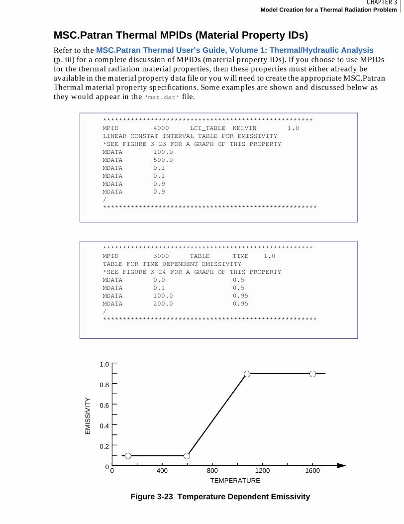
6CHAPTER 3Model Creation for a Thermal Radiation Problem
MSC.Patran Thermal MPIDs (Material Property IDs)Refer to the MSC.Patran Thermal User’s Guide, Volume 1: Thermal/Hydraulic Analysis (p. iii) for a complete discussion of MPIDs (material property IDs). If you choose to use MPIDs for the thermal radiation material properties, then these properties must either already be available in the material property data file or you will need to create the appropriate MSC.Patran Thermal material property specifications. Some examples are shown and discussed below as they would appear in the ‘mat.dat’ file.
Figure 3-23 Temperature Dependent Emissivity
*****************************************************MPID 4000 LCI_TABLE KELVIN 1.0LINEAR CONSTAT INTERVAL TABLE FOR EMISSIVITY*SEE FIGURE 3-23 FOR A GRAPH OF THIS PROPERTYMDATA 100.0MDATA 500.0MDATA 0.1MDATA 0.1MDATA 0.9MDATA 0.9/******************************************************
*****************************************************MPID 3000 TABLE TIME 1.0TABLE FOR TIME DEPENDENT EMISSIVITY*SEE FIGURE 3-24 FOR A GRAPH OF THIS PROPERTYMDATA 0.0 0.5MDATA 0.1 0.5MDATA 100.0 0.95MDATA 200.0 0.95/******************************************************
0 400 800 1200 16000
0.2
0.4
0.6
0.8
1.0
TEMPERATURE
EM
ISS
IVIT
Y
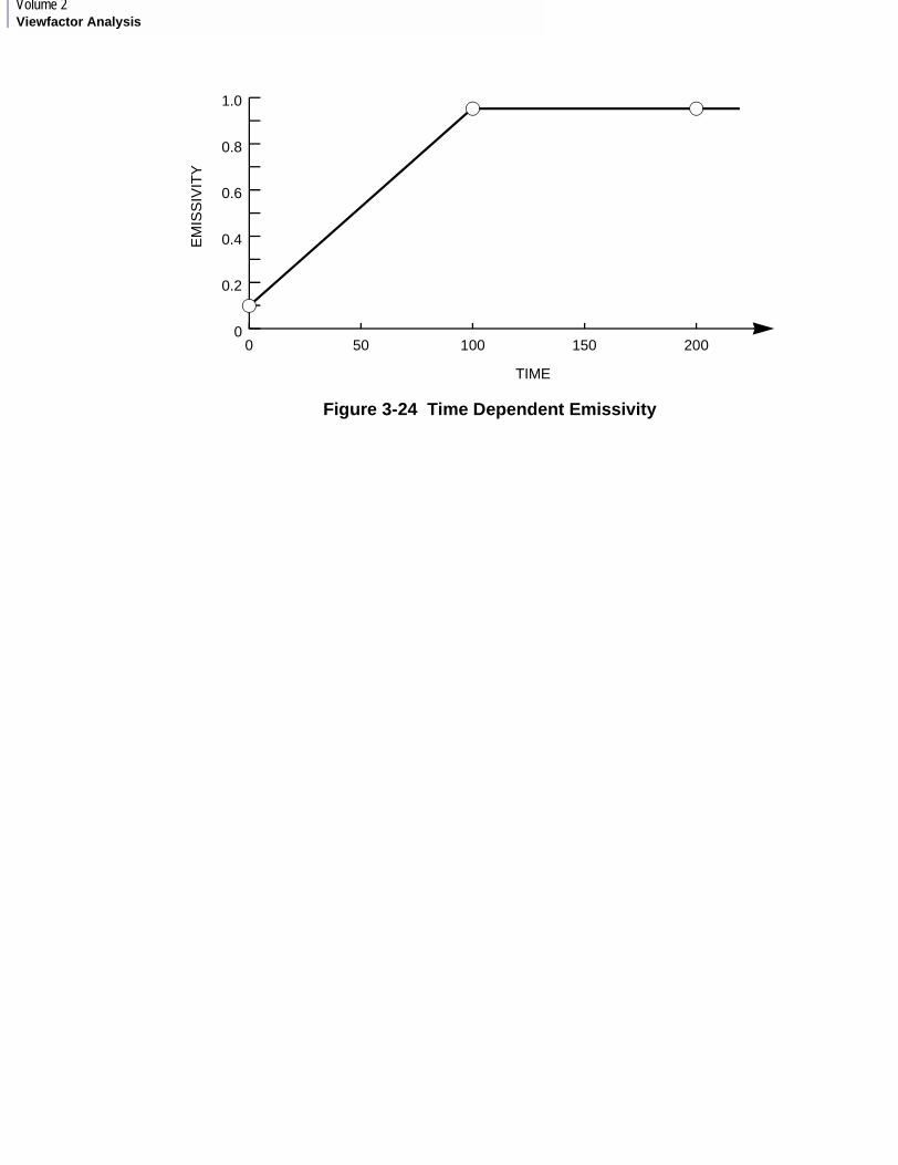
Volume 2Viewfactor Analysis
Figure 3-24 Time Dependent Emissivity
0 50 100 150 2000
0.2
0.4
0.6
0.8
1.0
TIME
EM
ISS
IVIT
Y
6CHAPTER 3Model Creation for a Thermal Radiation Problem
MSC.Patran Thermal Material Property DefinitionThe various ways to define material properties are described in the MSC.Patran Thermal User’s Guide. Note that by referencing the MPID as a negative number in the TEMPLATEDAT template the material property will be evaluated as a function of time instead of as a function of temperature.
In MSC.Patran, the material properties in MSC.Patran Thermal MPIDs (Material Property IDs) (p. 65) are defined under fields:
Click on Input Data, then the desired MSC.Patran Thermal material function (e.g., "mpid_linr_tabl" will bring up the input data for a tabular input).
Finite Element
Action: Create
Object: Material Property
Method: General
Note: Make sure you have selected MSC.Patran Thermal as the analysis preference.
Volume 2Viewfactor Analysis
VFAC Template FormatThe complete specification of the VFAC template is given in TEMPLATEDAT (Surface Pointer Data) (p. 160). Unless the reader plans to interface to the Viewfactor module formally through another computer code, the description of the VFAC template in this section will be all that is needed.
The VFAC template consists of a header line and one or more following data lines. Data on the header line will determine how many data lines must follow. Some of the data is optional, or optional depending on what other data is entered. All optional data defaults to standard values. If the value desired is the default value, then you need not enter the optional default values, as they will be assigned automatically.
KEYWORD TID nbands
The first line of the VFAC template, or header line, consists of three fields. These fields are:
1. The keyword VFAC,
2. Followed by the template ID number, TID, and finally
3. The number of wavebands and nbands used to define the thermal radiation properties. The first two fields are required and the third field is optional and defaults to zero. The TID and nbands must be integers. The fields should be separated by one or more spaces or by commas.
The number of data lines following the header line must be exactly the number of nbands, except that if the nbands field is blank or zero there must be exactly one data line following. Comments may also be placed at the end of header or data lines by placing a semicolon after the last data field on the line.
Some example header lines are:
which specifies that this is VFAC template 99 and represents a gray material property, and
which specifies that this is VFAC template 1001 and represents a material with 6 wavebands.
The data lines contain eight fields each. The fields are separated by one or more spaces or by commas. The first field, CONSTANT_EPSILON, is the only required field. Trailing blank fields may be omitted. Blank fields between nonblank fields are not permitted and will be ignored, thus corrupting the user’s data. The fields are:
CONSTANT_EPSILON, CONSTANT_TAU, EMPID, TMPID, LAMBDA1, LAMBDA2, KFLAG, COLLAPSE
TID Valid TIDs are positive integers. TIDs will be associated with UIDs from the MSC.Patran Viewfactor LBC form.
nbands Valid values of nbands are non-negative integers. If nbands is zero (the default), then this template will cause R-type resistors to be created; otherwise, W-type resistors will be created when this template is referenced.
VFAC 99
VFAC 1001 6
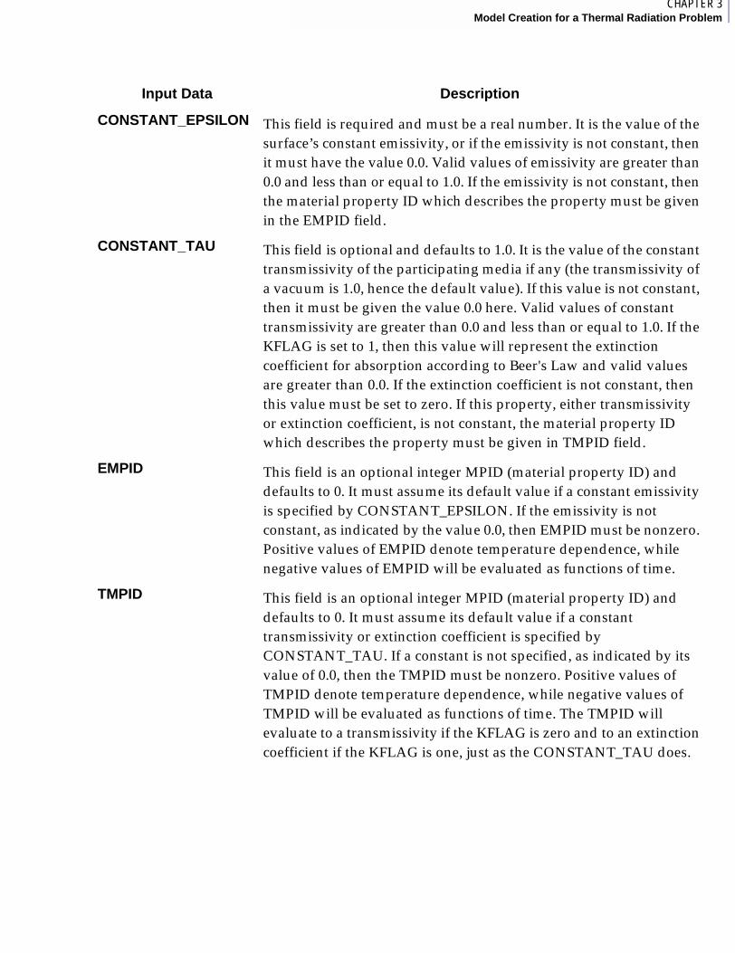
6CHAPTER 3Model Creation for a Thermal Radiation Problem
Input Data Description
CONSTANT_EPSILON This field is required and must be a real number. It is the value of the surface’s constant emissivity, or if the emissivity is not constant, then it must have the value 0.0. Valid values of emissivity are greater than 0.0 and less than or equal to 1.0. If the emissivity is not constant, then the material property ID which describes the property must be given in the EMPID field.
CONSTANT_TAU This field is optional and defaults to 1.0. It is the value of the constant transmissivity of the participating media if any (the transmissivity of a vacuum is 1.0, hence the default value). If this value is not constant, then it must be given the value 0.0 here. Valid values of constant transmissivity are greater than 0.0 and less than or equal to 1.0. If the KFLAG is set to 1, then this value will represent the extinction coefficient for absorption according to Beer's Law and valid values are greater than 0.0. If the extinction coefficient is not constant, then this value must be set to zero. If this property, either transmissivity or extinction coefficient, is not constant, the material property ID which describes the property must be given in TMPID field.
EMPID This field is an optional integer MPID (material property ID) and defaults to 0. It must assume its default value if a constant emissivity is specified by CONSTANT_EPSILON. If the emissivity is not constant, as indicated by the value 0.0, then EMPID must be nonzero. Positive values of EMPID denote temperature dependence, while negative values of EMPID will be evaluated as functions of time.
TMPID This field is an optional integer MPID (material property ID) and defaults to 0. It must assume its default value if a constant transmissivity or extinction coefficient is specified by CONSTANT_TAU. If a constant is not specified, as indicated by its value of 0.0, then the TMPID must be nonzero. Positive values of TMPID denote temperature dependence, while negative values of TMPID will be evaluated as functions of time. The TMPID will evaluate to a transmissivity if the KFLAG is zero and to an extinction coefficient if the KFLAG is one, just as the CONSTANT_TAU does.

Volume 2Viewfactor Analysis
LAMBDA1, LAMBDA2 These are optional real fields, but either they both must be present or both not present. They are the beginning and ending wavelengths for the present waveband. Note that the wavebands do not necessarily have to be in order of increasing wavelength but must be in the same order for every surface in an enclosure. These fields default to 0.0, the value for the case when nbands is 0. If nbands is greater than 0 (i.e., the properties have spectral dependence), then LAMBDA2 should be greater than LAMBDA1, which should be greater than 0.0. The units used for wavelength are microns or micrometers.
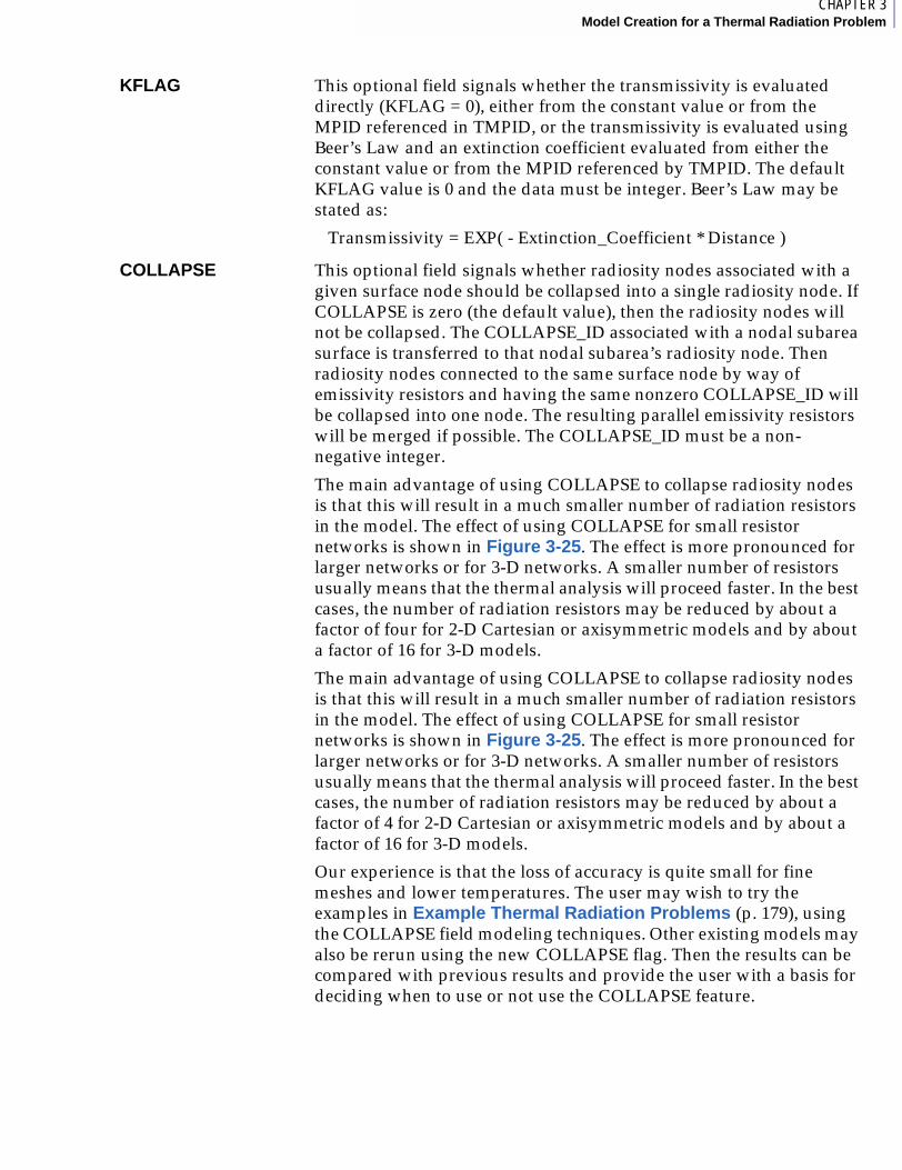
7CHAPTER 3Model Creation for a Thermal Radiation Problem
KFLAG This optional field signals whether the transmissivity is evaluated directly (KFLAG = 0), either from the constant value or from the MPID referenced in TMPID, or the transmissivity is evaluated using Beer’s Law and an extinction coefficient evaluated from either the constant value or from the MPID referenced by TMPID. The default KFLAG value is 0 and the data must be integer. Beer’s Law may be stated as:
Transmissivity = EXP( - Extinction_Coefficient * Distance )
COLLAPSE This optional field signals whether radiosity nodes associated with a given surface node should be collapsed into a single radiosity node. If COLLAPSE is zero (the default value), then the radiosity nodes will not be collapsed. The COLLAPSE_ID associated with a nodal subarea surface is transferred to that nodal subarea’s radiosity node. Then radiosity nodes connected to the same surface node by way of emissivity resistors and having the same nonzero COLLAPSE_ID will be collapsed into one node. The resulting parallel emissivity resistors will be merged if possible. The COLLAPSE_ID must be a non-negative integer.
The main advantage of using COLLAPSE to collapse radiosity nodes is that this will result in a much smaller number of radiation resistors in the model. The effect of using COLLAPSE for small resistor networks is shown in Figure 3-25. The effect is more pronounced for larger networks or for 3-D networks. A smaller number of resistors usually means that the thermal analysis will proceed faster. In the best cases, the number of radiation resistors may be reduced by about a factor of four for 2-D Cartesian or axisymmetric models and by about a factor of 16 for 3-D models.
The main advantage of using COLLAPSE to collapse radiosity nodes is that this will result in a much smaller number of radiation resistors in the model. The effect of using COLLAPSE for small resistor networks is shown in Figure 3-25. The effect is more pronounced for larger networks or for 3-D networks. A smaller number of resistors usually means that the thermal analysis will proceed faster. In the best cases, the number of radiation resistors may be reduced by about a factor of 4 for 2-D Cartesian or axisymmetric models and by about a factor of 16 for 3-D models.
Our experience is that the loss of accuracy is quite small for fine meshes and lower temperatures. The user may wish to try the examples in Example Thermal Radiation Problems (p. 179), using the COLLAPSE field modeling techniques. Other existing models may also be rerun using the new COLLAPSE flag. Then the results can be compared with previous results and provide the user with a basis for deciding when to use or not use the COLLAPSE feature.
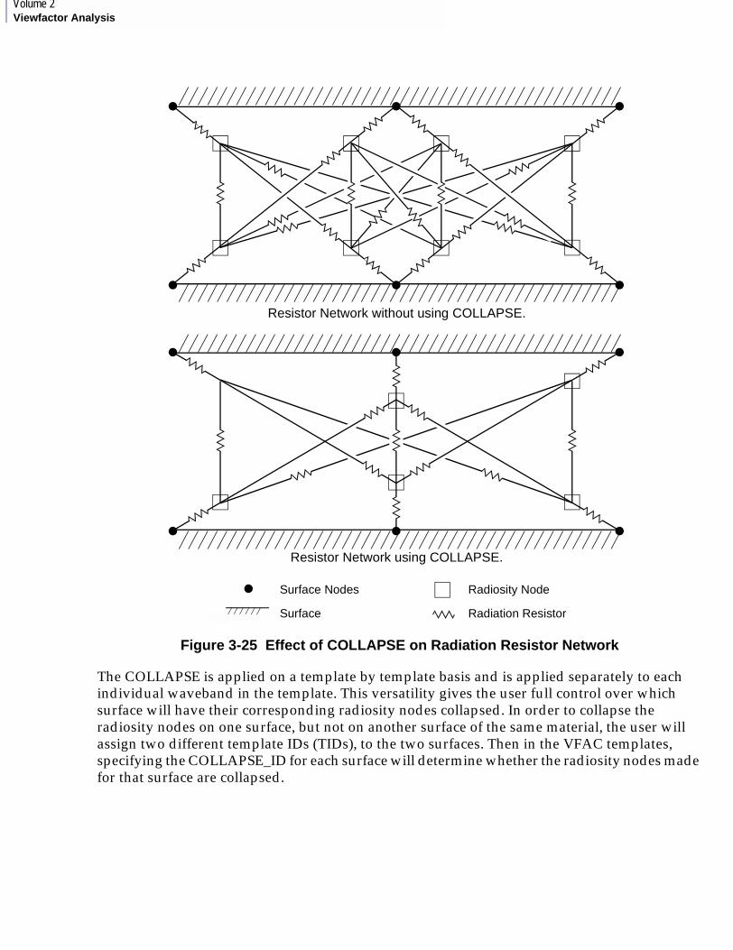
Volume 2Viewfactor Analysis
Figure 3-25 Effect of COLLAPSE on Radiation Resistor Network
The COLLAPSE is applied on a template by template basis and is applied separately to each individual waveband in the template. This versatility gives the user full control over which surface will have their corresponding radiosity nodes collapsed. In order to collapse the radiosity nodes on one surface, but not on another surface of the same material, the user will assign two different template IDs (TIDs), to the two surfaces. Then in the VFAC templates, specifying the COLLAPSE_ID for each surface will determine whether the radiosity nodes made for that surface are collapsed.
Surface Nodes
Surface
Radiosity Node
Radiation Resistor
Resistor Network using COLLAPSE.
Resistor Network without using COLLAPSE.
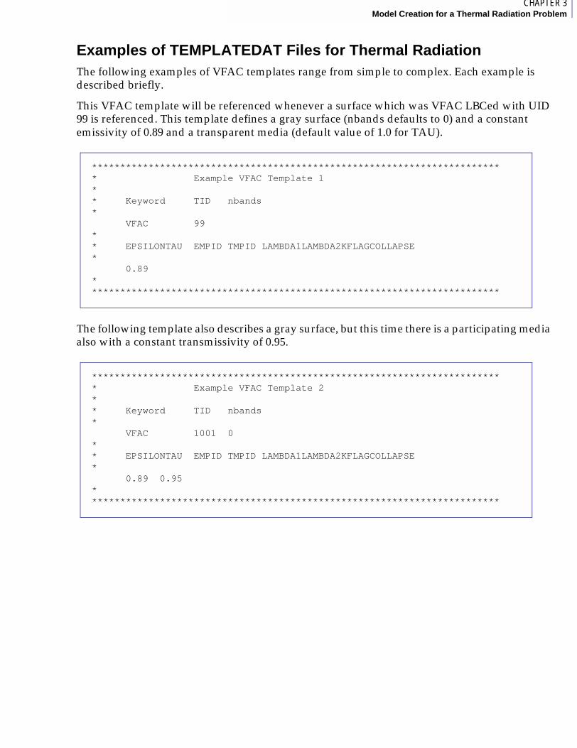
7CHAPTER 3Model Creation for a Thermal Radiation Problem
Examples of TEMPLATEDAT Files for Thermal RadiationThe following examples of VFAC templates range from simple to complex. Each example is described briefly.
This VFAC template will be referenced whenever a surface which was VFAC LBCed with UID 99 is referenced. This template defines a gray surface (nbands defaults to 0) and a constant emissivity of 0.89 and a transparent media (default value of 1.0 for TAU).
The following template also describes a gray surface, but this time there is a participating media also with a constant transmissivity of 0.95.
************************************************************************* Example VFAC Template 1** Keyword TID nbands*
VFAC 99** EPSILONTAU EMPID TMPID LAMBDA1LAMBDA2KFLAGCOLLAPSE*
0.89*************************************************************************
************************************************************************* Example VFAC Template 2** Keyword TID nbands*
VFAC 1001 0** EPSILONTAU EMPID TMPID LAMBDA1LAMBDA2KFLAGCOLLAPSE*
0.89 0.95*************************************************************************
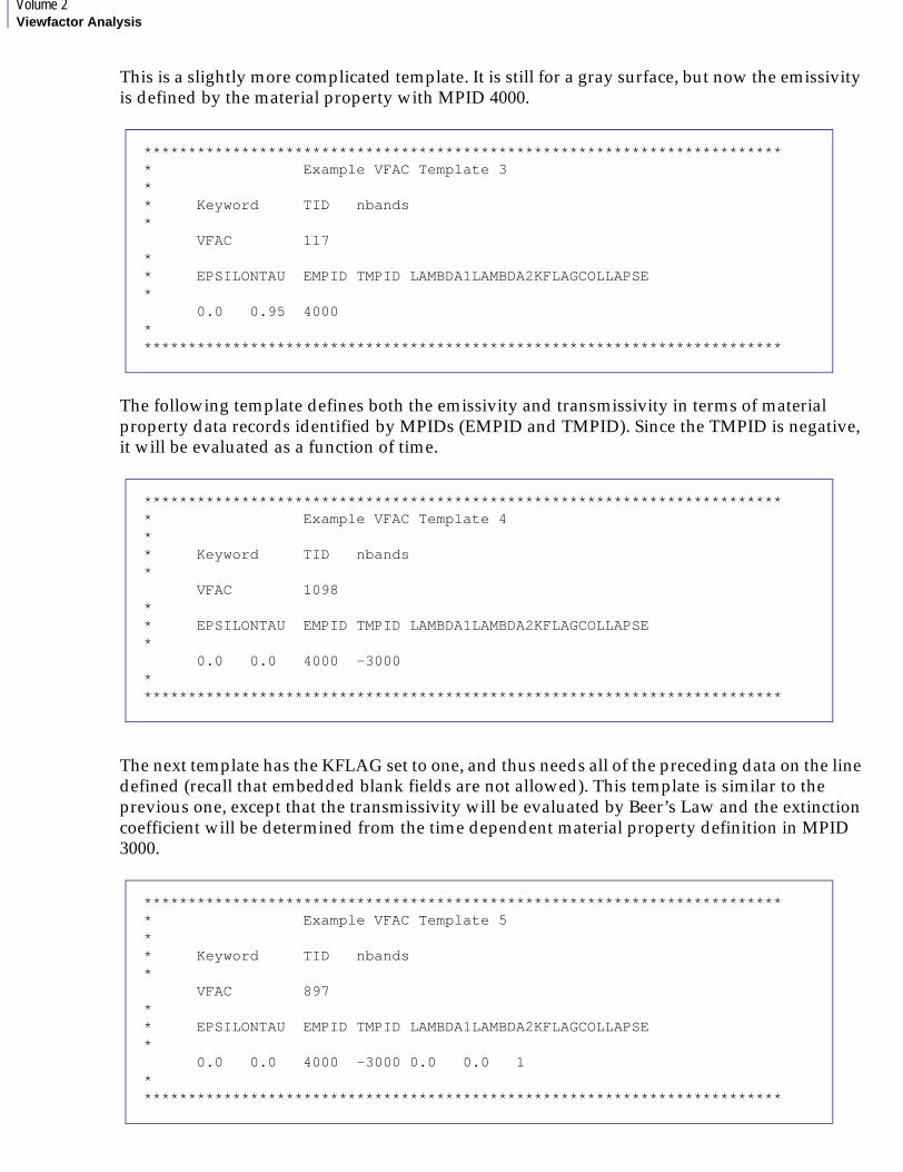
Volume 2Viewfactor Analysis
This is a slightly more complicated template. It is still for a gray surface, but now the emissivity is defined by the material property with MPID 4000.
The following template defines both the emissivity and transmissivity in terms of material property data records identified by MPIDs (EMPID and TMPID). Since the TMPID is negative, it will be evaluated as a function of time.
The next template has the KFLAG set to one, and thus needs all of the preceding data on the line defined (recall that embedded blank fields are not allowed). This template is similar to the previous one, except that the transmissivity will be evaluated by Beer’s Law and the extinction coefficient will be determined from the time dependent material property definition in MPID 3000.
************************************************************************* Example VFAC Template 3** Keyword TID nbands*
VFAC 117** EPSILONTAU EMPID TMPID LAMBDA1LAMBDA2KFLAGCOLLAPSE*
0.0 0.95 4000*************************************************************************
************************************************************************* Example VFAC Template 4** Keyword TID nbands*
VFAC 1098** EPSILONTAU EMPID TMPID LAMBDA1LAMBDA2KFLAGCOLLAPSE*
0.0 0.0 4000 -3000*************************************************************************
************************************************************************* Example VFAC Template 5** Keyword TID nbands*
VFAC 897** EPSILONTAU EMPID TMPID LAMBDA1LAMBDA2KFLAGCOLLAPSE*
0.0 0.0 4000 -3000 0.0 0.0 1*************************************************************************
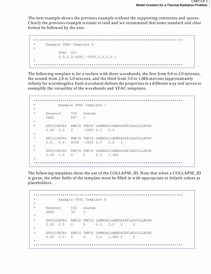
7CHAPTER 3Model Creation for a Thermal Radiation Problem
The next example shows the previous example without the supporting comments and spaces. Clearly the previous example is easier to read and we recommend that some standard and clear format be followed by the user.
The following template is for a surface with three wavebands, the first from 0.0 to 2.0 microns, the second from 2.0 to 5.0 microns, and the third from 5.0 to 1.0E6 microns (approximately infinity for wavelengths). Each waveband defines the properties in a different way and serves to exemplify the versatility of the wavebands and VFAC templates.
The following templates show the use of the COLLAPSE_ID. Note that when a COLLAPSE_ID is given, the other fields of the template must be filled in with appropriate or default values as placeholders.
************************************************************************* Example VFAC Template 6*
VFAC 8970.0,0.0,4000,-3000,0.0,0.0,1
*************************************************************************
************************************************************************* Example VFAC Template 7** Keyword TID nbands
VFAC 897 3** EPSILONTAU EMPID TMPID LAMBDA1LAMBDA2KFLAGCOLLAPSE
0.89 0.0 0 -3000 0.0 2.0** EPSILONTAU EMPID TMPID LAMBDA1LAMBDA2KFLAGCOLLAPSE
0.0. 0.0 4000 -3000 2.0 5.0 1** EPSILONTAU EMPID TMPID LAMBDA1LAMBDA2KFLAGCOLLAPSE
0.98 1.0 0 0 5.0 1.0E6*************************************************************************
************************************************************************* Example VFAC Template 8** Keyword TID nbands
VFAC 39 2** EPSILONTAU EMPID TMPID LAMBDA1LAMBDA2KFLAGCOLLAPSE
0.00 0.0 0 0 0.0 3.0 0 0** EPSILONTAU EMPID TMPID LAMBDA1LAMBDA2KFLAGCOLLAPSE
0.00 0.0 0 0 3.0 1.0E6 0 2*************************************************************************
Volume 2Viewfactor Analysis
3.8 Compatibility Requirements for Model and VFAC TemplatesThe model of the problem and its VFAC boundary condition data must satisfy certain compatibility requirements or else an error will occur in Viewfactor while attempting to combine the viewfactor data and the VFAC template data to make resistors. Should this occur, you may need to change the VFAC boundary condition and rerun the viewfactor analysis. The best way to avoid this is careful planning.
Origin of the ProblemThe compatibility requirements primarily originate from the fact that thermal radiation interchange is between pairs of surfaces and the requirement in MSC.Patran Thermal that the radiation resistors be symmetric. Thus, the resistor that would be made from surface one to surface two must be the same as would be made from surface two to surface one. Which resistors are made is determined by the VFAC template data and VFAC boundary condition data for each surface. Incompatibility results, for example, when one surface is gray (nbands = 0) and the other surface has spectral wavebands (nbands > 0).
Compatibility problems can also arise just from a single surface and its associated VFAC data. An example of this is a VFAC boundary condition with an AMBNOD specified and a VFAC template with KFLAG set to one. The problem here is that the KFLAG setting will require a distance for calculating the transmissivity from Beer’s Law and the distance from the surface to the ambient environment (AMBNOD) is not well defined or known.
The specific compatibility requirements are:
• All UIDs referenced in the VFAC boundary condition, input data form must be available TIDs in the VFAC templates.
• All VFAC templates referenced by the VFAC boundary condition UIDs in an enclosure must have the same number of wavebands. This means that all surfaces in an enclosure must either be gray (nbands = 0) or have the same spectral wavebands (nbands > 0).
• Surfaces with an AMBNOD in their VFAC LBC are incompatible with VFAC templates that have their KFLAG set to one. If the user wishes to model the problem with KFLAG set to one, then the ambient environment must be modeled as surfaces at the ambient temperature.
• If the surface has not been given a participating media node, MEDNOD, in its VFAC boundary condition and the constant transmissivity, CONSTANT_TAU, is not set to 1.0 in the VFAC template identified by the UID for that surface, then an error will occur. This is because no participating media has been defined, yet the VFAC template says that some of the radiant energy from the surface is absorbed by the medium (since the transmissivity is not 1.0).
• For every pair of surfaces in an enclosure that can see each other, the following quantities for each must be equal:
MEDNOD, CONSTANT_TAU, TMPID, LAMBDA1, LAMBDA2, and KFLAG.
• If there are multiple wavebands, then this condition must hold for each waveband. Note also that by the previous requirement on wavebands in the enclosure that the number of wavebands for every pair of surfaces which can see each other is equal.

7CHAPTER 3Model Creation for a Thermal Radiation Problem
Suggested Procedures to Avoid Compatibility ProblemsCareful planning is the key to avoiding compatibility problems between the model’s VFAC boundary condition data and the VFAC templates in the TEMPLATEDAT file. Plan out the modeling strategy, paying particular attention to the most complex model of the problem. If for example, a simple model does not include a participating media node even though it is not used, the viewfactor calculations will have to be redone if in the future a participating media needs to be modeled. If, on the other hand, the participating media node had been included in the model, even though it will not be used in the simple model when it is needed in the more complex model with the participating media, it will be there and the viewfactors will not have to be recalculated. Only the VFAC templates will need to be changed and new MSC.Patran Thermal radiation resistors made.
If you plan or want to be able to use the KFLAG set equal to one option, then do not use ambient environment nodes, AMBNOD, in the model. Instead, model the ambient environment as surfaces at the ambient temperature.
If you plan or want to be able to model participating media, include the participating media node, MEDNOD, in the model. There is no harm if it is not used, but it will be there when it is needed.
Take care when planning the enclosures and participating media nodes, MEDNOD, to ensure that all surface pairs in an enclosure which can see each other have the same MEDNOD.
The above suggestions are the most important, as failure to follow them may require that the viewfactors be recalculated and this is the most computationally expensive part of the Viewfactor analysis.
The requirements for the equality of the CONSTANT_TAU, TMPID, LAMBDA1, LAMBDA2, and KFLAG between surface pairs which can see each other in an enclosure is not so troublesome if violated. It can be corrected by changing the VFAC templates but does not in general require recalculating the viewfactors. Still, careful planning is the best prevention. If there are two or more enclosures, the user may wish to use different VFAC templates for the same material in the different enclosures. This will give the user greater latitude in modeling different, but simultaneous, phenomena in the different enclosures.
If a constant value for transmissivity, CONSTANT_TAU, is used, it must be the same for all surfaces in an enclosure which can see each other.
The TMPID must be the same for all surfaces in an enclosure which can see each other.
The KFLAG must be the same for all surfaces in an enclosure which can see each other.
If the KFLAG is zero, then the CONSTANT_TAU or TMPID data must be for transmissivity data directly. If the KFLAG is one, then the CONSTANT_TAU or TMPID data must be for extinction coefficient data to be used in Beer’s Law.
The beginning and ending wavelengths for each waveband in the enclosure must be in the same order and must be equal for all surfaces in an enclosure which can see each other.
Given these restrictions on the data in an enclosure, the user may wish to model the same material in each different enclosure with different UIDs so that for example it may be represented with different VFAC templates in each different enclosure. This involves some additional work, but greatly extends the flexibility and capabilities of the model.
Volume 2Viewfactor Analysis
3.9 Symmetry as Applied to the Model and Viewfactor Radiation ExchangeSymmetry as it relates to viewfactors and thermal radiation analysis is not a very easy topic to understand. If the user does not plan to make use of symmetry in modeling the problem, then this section may be omitted from study. Also, the user may wish to come back to this section at a later time, after mastering other aspects of viewfactor analysis, since this material is not in the mainstream of the rest of this document. The symmetry which we refer to here is not the symmetry of axisymmetry or the symmetry which allows us to reduce a three-dimensional model to a two-dimensional model. Rather it is the symmetry which pertains to reflections about lines or planes and discrete rotations about an axis.
The Purpose of Symmetry in ViewfactorWhen modeling thermal problems the analyst may look for and make use of symmetry in the model geometry, materials, and boundary conditions. This is typically done to reduce the overall size of the computer descriptions of the problem and reduce the time required to analyze it. There are many existing models for particular thermal problems and many of them have made use of symmetry in describing the problem. It is advantageous, to the greatest extent reasonably possible, to be able to use these existing models for thermal radiation analysis also.
Unfortunately, this is frequently not possible because the radiative boundary condition imposes a much stricter symmetry requirement on the model than do the other boundary conditions, material properties or geometry. The other boundary conditions typically involve only one surface area at a time, whereas the radiative energy interchange at the boundary involves pairs of surface areas and complicated relationships between the surface’s normals, angles between these normals and the intersurface ray, and the distance between the surfaces. In order for the model to possess true symmetry, all of these attributes must exhibit the same symmetry and this is usually not the case.
It is desirable not to make a full model of an otherwise symmetric model just to deal with the nonsymmetry imposed by the radiative boundary conditions. To this end, Viewfactor provides some capabilities for specifying symmetry for the viewfactor analysis that is only needed for the Viewfactor analysis and not needed for the remainder of the thermal analysis. This will allow the use of existing models, in some cases, with only minor modification (addition of the symmetry information), and allows the thermal network analysis to be performed on the symmetric model while the viewfactor calculations are performed on the complete model.
Caveats Concerning the Use of Symmetry in Thermal Radiation ModelingMSC.Patran and Viewfactor cannot check the validity of the user’s symmetry description of the model. When ascertaining the nature of the symmetry present (or not present as the case may be) for thermal radiation interchange and viewfactors, there is ample opportunity for error. These errors are often difficult to detect either by inspection of the model or from detecting erroneous analysis results. We are generally not used to thinking in terms of the symmetry requirements for viewfactors between pairs of surfaces and so this symmetry, or lack thereof, is not intuitively obvious to us as is say geometric symmetry. Frequently we work with problems so complex that we are unable to known whether the analysis is correct or not and thus cannot rely on the detection of erroneous results to detect symmetry errors. Some examples are given later in this section to illustrate the difficulty of correctly modeling symmetry for radiative boundary conditions.
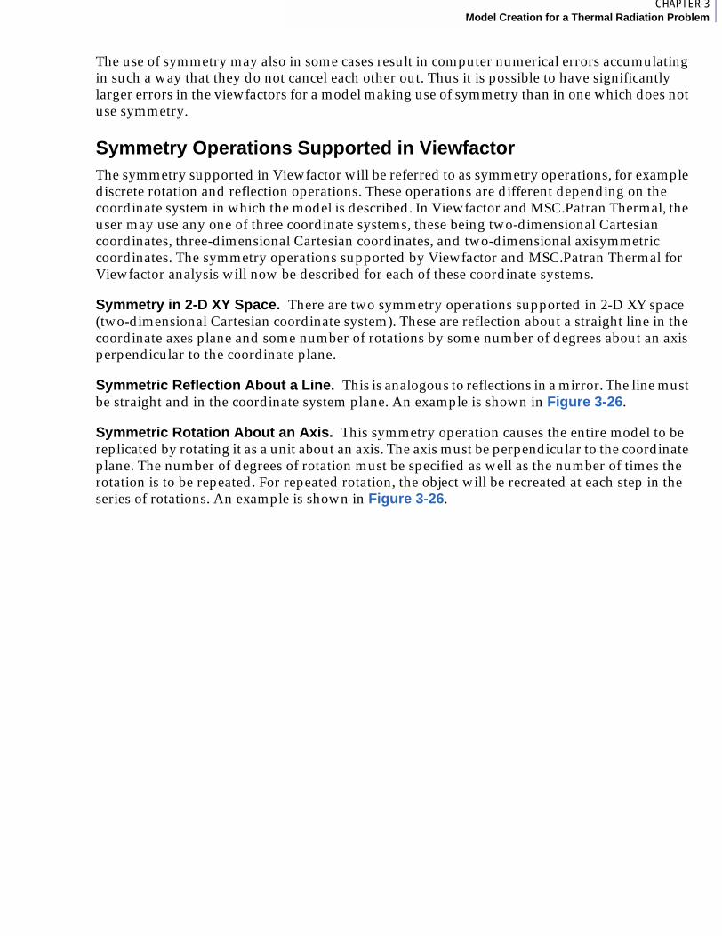
7CHAPTER 3Model Creation for a Thermal Radiation Problem
The use of symmetry may also in some cases result in computer numerical errors accumulating in such a way that they do not cancel each other out. Thus it is possible to have significantly larger errors in the viewfactors for a model making use of symmetry than in one which does not use symmetry.
Symmetry Operations Supported in ViewfactorThe symmetry supported in Viewfactor will be referred to as symmetry operations, for example discrete rotation and reflection operations. These operations are different depending on the coordinate system in which the model is described. In Viewfactor and MSC.Patran Thermal, the user may use any one of three coordinate systems, these being two-dimensional Cartesian coordinates, three-dimensional Cartesian coordinates, and two-dimensional axisymmetric coordinates. The symmetry operations supported by Viewfactor and MSC.Patran Thermal for Viewfactor analysis will now be described for each of these coordinate systems.
Symmetry in 2-D XY Space. There are two symmetry operations supported in 2-D XY space (two-dimensional Cartesian coordinate system). These are reflection about a straight line in the coordinate axes plane and some number of rotations by some number of degrees about an axis perpendicular to the coordinate plane.
Symmetric Reflection About a Line. This is analogous to reflections in a mirror. The line must be straight and in the coordinate system plane. An example is shown in Figure 3-26.
Symmetric Rotation About an Axis. This symmetry operation causes the entire model to be replicated by rotating it as a unit about an axis. The axis must be perpendicular to the coordinate plane. The number of degrees of rotation must be specified as well as the number of times the rotation is to be repeated. For repeated rotation, the object will be recreated at each step in the series of rotations. An example is shown in Figure 3-26.
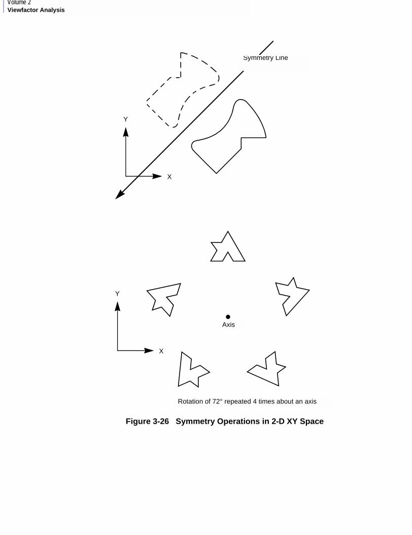
Volume 2Viewfactor Analysis
Figure 3-26 Symmetry Operations in 2-D XY Space
X
Y
X
Y
Symmetry Line
Axis
Rotation of 72° repeated 4 times about an axis
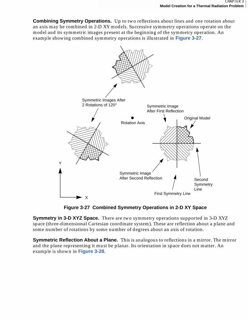
8CHAPTER 3Model Creation for a Thermal Radiation Problem
Combining Symmetry Operations. Up to two reflections about lines and one rotation about an axis may be combined in 2-D XY models. Successive symmetry operations operate on the model and its symmetric images present at the beginning of the symmetry operation. An example showing combined symmetry operations is illustrated in Figure 3-27.
Figure 3-27 Combined Symmetry Operations in 2-D XY Space
Symmetry in 3-D XYZ Space. There are two symmetry operations supported in 3-D XYZ space (three-dimensional Cartesian coordinate system). These are reflection about a plane and some number of rotations by some number of degrees about an axis of rotation.
Symmetric Reflection About a Plane. This is analogous to reflections in a mirror. The mirror and the plane representing it must be planar. Its orientation in space does not matter. An example is shown in Figure 3-28.
X
Y
Symmetric ImageAfter Second Reflection
First Symmetry Line
SecondSymmetryLine
Symmetric ImageAfter First Reflection
Original ModelRotation Axis
Symmetric Images After2 Rotations of 120°
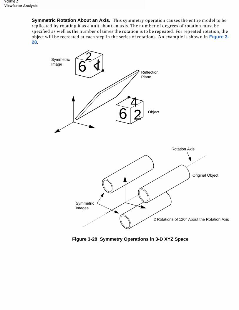
Volume 2Viewfactor Analysis
Symmetric Rotation About an Axis. This symmetry operation causes the entire model to be replicated by rotating it as a unit about an axis. The number of degrees of rotation must be specified as well as the number of times the rotation is to be repeated. For repeated rotation, the object will be recreated at each step in the series of rotations. An example is shown in Figure 3-28.
Figure 3-28 Symmetry Operations in 3-D XYZ Space
2 Rotations of 120° About the Rotation Axis
Original Object
Rotation Axis
SymmetricImages
Object
ReflectionPlane
SymmetricImage
642
62
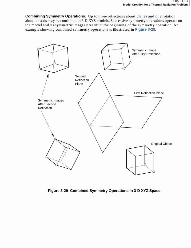
8CHAPTER 3Model Creation for a Thermal Radiation Problem
Combining Symmetry Operations. Up to three reflections about planes and one rotation about an axis may be combined in 3-D XYZ models. Successive symmetry operations operate on the model and its symmetric images present at the beginning of the symmetry operation. An example showing combined symmetry operations is illustrated in Figure 3-29.
Figure 3-29 Combined Symmetry Operations in 3-D XYZ Space
Symmetric Images After Second Reflection
Second Reflection Plane
Symmetric ImageAfter First Reflection
First Reflection Plane
Original Object
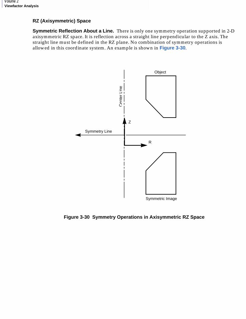
Volume 2Viewfactor Analysis
RZ (Axisymmetric) Space
Symmetric Reflection About a Line. There is only one symmetry operation supported in 2-D axisymmetric RZ space. It is reflection across a straight line perpendicular to the Z axis. The straight line must be defined in the RZ plane. No combination of symmetry operations is allowed in this coordinate system. An example is shown in Figure 3-30.
Figure 3-30 Symmetry Operations in Axisymmetric RZ Space
Symmetry Line
Object
Cen
ter
Line
Symmetric Image
Z
R
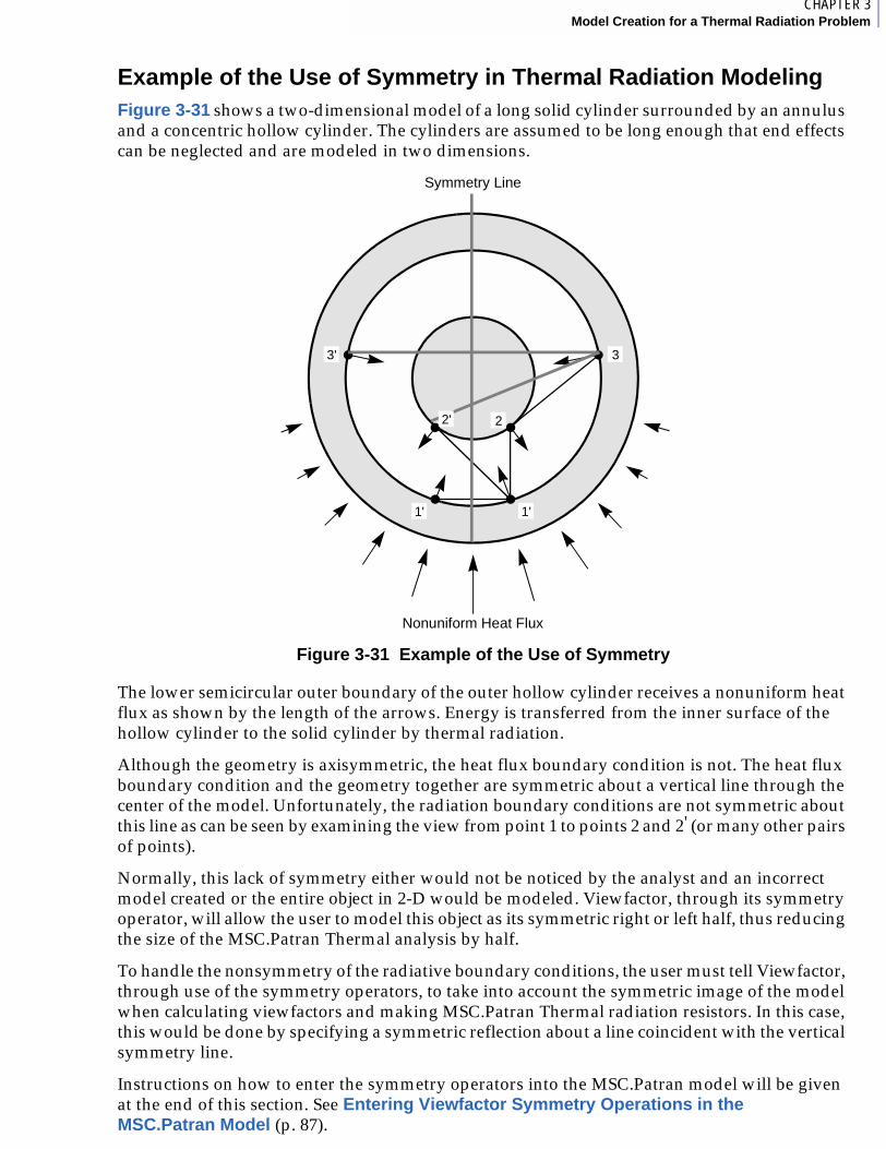
8CHAPTER 3Model Creation for a Thermal Radiation Problem
Example of the Use of Symmetry in Thermal Radiation ModelingFigure 3-31 shows a two-dimensional model of a long solid cylinder surrounded by an annulus and a concentric hollow cylinder. The cylinders are assumed to be long enough that end effects can be neglected and are modeled in two dimensions.
Figure 3-31 Example of the Use of Symmetry
The lower semicircular outer boundary of the outer hollow cylinder receives a nonuniform heat flux as shown by the length of the arrows. Energy is transferred from the inner surface of the hollow cylinder to the solid cylinder by thermal radiation.
Although the geometry is axisymmetric, the heat flux boundary condition is not. The heat flux boundary condition and the geometry together are symmetric about a vertical line through the center of the model. Unfortunately, the radiation boundary conditions are not symmetric about this line as can be seen by examining the view from point 1 to points 2 and 2' (or many other pairs of points).
Normally, this lack of symmetry either would not be noticed by the analyst and an incorrect model created or the entire object in 2-D would be modeled. Viewfactor, through its symmetry operator, will allow the user to model this object as its symmetric right or left half, thus reducing the size of the MSC.Patran Thermal analysis by half.
To handle the nonsymmetry of the radiative boundary conditions, the user must tell Viewfactor, through use of the symmetry operators, to take into account the symmetric image of the model when calculating viewfactors and making MSC.Patran Thermal radiation resistors. In this case, this would be done by specifying a symmetric reflection about a line coincident with the vertical symmetry line.
Instructions on how to enter the symmetry operators into the MSC.Patran model will be given at the end of this section. See Entering Viewfactor Symmetry Operations in the MSC.Patran Model (p. 87).
Nonuniform Heat Flux
Symmetry Line
3' 3
1' 1'
22'

Volume 2Viewfactor Analysis
Example Which Appears Symmetric, But in Fact Is Not SymmetricThis example is similar to the previous example except the heat flux boundary condition has been changed to be symmetric on a quarter section of the model. One way to model this problem appears to be to take the upper right quarter section and replicate it by rotating about the center point by 90 degrees and then reflecting the resulting model and image about a horizontal line through the cylinder’s center as shown in Figure 3-32.
Figure 3-32 Incorrect Use of Symmetry Operations in Viewfactor
The geometry and boundary conditions seemingly appear as we think they should. You might be tempted to define a Viewfactor rotational symmetry operator and reflection symmetry operator for this problem and proceed with the thermal analysis using the quarter section model. This, however, would be erroneous.
Upon careful examination of the model the reader can see that, for example, the view from point 1 is not the same as the view from point 1''. Thus this is not a correct model of the radiative interchange in this model.
Such errors are subtle and difficult to detect. In general, we recommend that symmetry not be used in thermal radiation models in order to preclude the possibility of such problems.
2'
2'''
1'''2'''
1''
1
21'
3'
3
3''
3'''
8CHAPTER 3Model Creation for a Thermal Radiation Problem
Entering Viewfactor Symmetry Operations in the MSC.Patran ModelThe symmetry operators for Viewfactor are entered into the model through MSC.Patran as special elements. MSC.Patran Thermal’s PATQ then translates these special elements into Viewfactor symmetry operators. The symmetry operators, their relationship to the thermal model, and the images of the model they cause to be created in the Viewfactor program are described in The Purpose of Symmetry in Viewfactor (p. 78) through Symmetry Operations Supported in Viewfactor (p. 79). This section describes the mechanics of entering the special elements used to describe the symmetry operators in MSC.Patran. The meaning and proper use of the symmetry operators is explained in the previous sections.
The symmetry operators and their corresponding special elements are:
The element property data for rotation about an axis contains the number of times the rotation is to be repeated and the angle of rotation in degrees. The element input property form is found under Element Properties looks like
Get the Input Properties form under Element Properties.
The nodes belonging to the radiation symmetry elements have to be declared as type "I" nodes. To do so one must first create OD elements at the location of the nodes belonging to the radiation symmetry elements. When the OD elements are created go to the element properties menu and select dimension: OD, type: Node type and click on the ‘input data’ button and select ‘information node’ in the ‘node type’ data box. Then select the OD elements created as the application region and click on ‘apply’. Nodes of type I (ignore) will not be translated by PATQ into the MSC.Patran Thermal nodes, but will only be used by PATQ to generate the Viewfactor symmetry operators.
Reflection about a Plane Radiation Symmetry Triangle Element.
Reflection about a Line Radiation Symmetry Bar Element--Reflection.
Rotation about an Axis Radiation Symmetry Bar Element Rotation with element property data.
Finite Element
Action: Create
Object: ID
Type: Rad Sym Bar Rotation

MSC.Patran Thermal User’s Guide, Volume 2: Viewfactor Analysis
CHAPTER
4 Preparation for Analysis
■ Introduction
■ Viewfactor Execution From MSC.Patran Thermal
■ PATQ Translation from the MSC.Patran Neutral File to the VFINDAT File
■ VFCTL, the Viewfactor Program Execution Control File

Volume 2Viewfactor Analysis
4.1 IntroductionAfter the model has been created in MSC.Patran and output to a neutral file, you can proceed with the next step in the analysis cycle. This chapter addresses two topics:
1. Translating the MSC.Patran neutral file into a file, VFINDAT, which can be read by Viewfactor for analysis, and
2. Creating the Viewfactor program execution control file, VFCTL.
8CHAPTER 4Preparation for Analysis
4.2 Viewfactor Execution From MSC.Patran ThermalThe Viewfactor run is submitted from the MSC.Patran Analysis form. The analysis preference must be set to MSC.Patran Thermal. To submit the run:
1. Make sure action is set to analyze in the Analysis form.
2. Under solution type, click Perform Viewfactor Analysis, OK to enter.
3. Under Solution Parameters, the Run Control Parameters and Viewfactor File Names may be selected. Default values have been assigned which should work for the majority of cases. (See Keywords in the VFCTL File (p. 98) for the parameter definition.)
4. Under Submit Options, make sure the Execute Viewfactor and Spawn Batch Job toggle are set (defaults).
After clicking, Apply on the Analysis form, the appropriate files will be created and a background job will be submitted.
Note: If both Execute Viewfactor Analysis and Execute Thermal Analysis toggles are set, MSC.Patran Thermal will wait until the Viewfactor solution is done before proceeding with the thermal analysis.

Volume 2Viewfactor Analysis
4.3 PATQ Translation from the MSC.Patran Neutral File to the VFINDAT FileThe MSC.Patran Thermal User’s Guide provides more complete information on the MSC.Patran Thermal program PATQ. This Guide is only concerned with the aspects of PATQ which relate to translating a neutral file to a VFINDAT file.
Spawning From MSC.Patran vs. Stand-Alone ExecutionTypically, MSC.Patran Thermal jobs will be spawned directly from MSC.Patran, in which case the job control will have been defined based on the solution type and submit options selected in the Analysis form. There are occasions (for example, if the thermal solver resides on a different workstation or on a mainframe) where a stand-alone run is required. The following provides the steps in the translation program (PATQ) for a stand-alone run.
The translation process is fairly simple and PATQ is an interactive menu-driven program with prompts for user input when required. Many of the prompts have default values that will be used if just a carriage return is entered. PATQ also generates diagnostic error messages if it detects any problems with the neutral file data.

9CHAPTER 4Preparation for Analysis
Step-by-Step Procedure (Stand-Alone Execution)Translating a neutral file using PATQ is a fairly simple procedure. Bold text represents user input. Plain capitalized text is used to show computer response. Commands are entered by pressing the RETURN key. The following example details the steps needed to do the translation. These sessions were run on a VAX/VMS installation. If you have a different system, or have altered the standard installation, your sessions may be slightly different. Refer to the Operations Guide for your computer for the correct commands.
Note: The steps below are automatically performed as a background job when MSC.Patran Thermal execution is spawned from MSC.Patran.
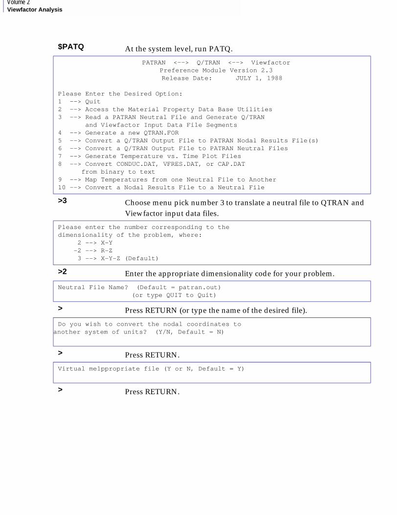
Volume 2Viewfactor Analysis
$PATQ At the system level, run PATQ.
PATRAN <--> Q/TRAN <--> Viewfactor Preference Module Version 2.3
Release Date: JULY 1, 1988
Please Enter the Desired Option:1 --> Quit2 --> Access the Material Property Data Base Utilities3 --> Read a PATRAN Neutral File and Generate Q/TRAN and Viewfactor Input Data File Segments4 --> Generate a new QTRAN.FOR5 --> Convert a Q/TRAN Output File to PATRAN Nodal Results File(s)6 --> Convert a Q/TRAN Output File to PATRAN Neutral Files7 --> Generate Temperature vs. Time Plot Files8 --> Convert CONDUC.DAT, VFRES.DAT, or CAP.DAT from binary to text9 --> Map Temperatures from one Neutral File to Another10 --> Convert a Nodal Results File to a Neutral File
>3 Choose menu pick number 3 to translate a neutral file to QTRAN and Viewfactor input data files.
Please enter the number corresponding to thedimensionality of the problem, where: 2 --> X-Y -2 --> R-Z 3 --> X-Y-Z (Default)
>2 Enter the appropriate dimensionality code for your problem.
Neutral File Name? (Default = patran.out) (or type QUIT to Quit)
> Press RETURN (or type the name of the desired file).
Do you wish to convert the nodal coordinates toanother system of units? (Y/N, Default = N)
> Press RETURN.
Virtual me1ppropriate file (Y or N, Default = Y)
> Press RETURN.
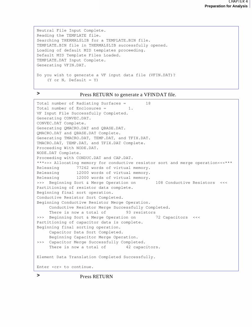
9CHAPTER 4Preparation for Analysis
Neutral File Input Complete.Reading the TEMPLATE file.Searching THERMAL$LIB for a TEMPLATE.BIN file.TEMPLATE.BIN file in THERMAL$LIB successfully opened.Loading of default MID templates proceeding.Default MID Template Files Loaded.TEMPLATE.DAT Input Complete.Generating VFIN.DAT. Do you wish to generate a VF input data file (VFIN.DAT)? (Y or N, Default = Y)
> Press RETURN to generate a VFINDAT file.
Total number of Radiating Surfaces = 18Total number of Enclosures = 1.VF Input File Successfully Completed.Generating CONVEC.DAT.CONVEC.DAT Complete.Generating QMACRO.DAT and QBASE.DAT.QMACRO.DAT and QBASE.DAT Complete.Generating TMACRO.DAT, TEMP.DAT, and TFIX.DAT.TMACRO.DAT, TEMP.DAT, and TFIX.DAT Complete.Proceeding With NODE.DAT.NODE.DAT Complete.Proceeding with CONDUC.DAT and CAP.DAT.***>>> Allocating memory for conductive resistor sort and merge operation<<<***Releasing 77262 words of virtual memory.Releasing 12000 words of virtual memory.Releasing 12000 words of virtual memory.>>> Beginning Sort & Merge Operation on 108 Conductive Resistors <<<Partitioning of resistor data complete.Beginning final sort operation.Conductive Resistor Sort Completed.Beginning Conductive Resistor Merge Operation. Conductive Resistor Merge Successfully Completed. There is now a total of 93 resistors>>> Beginning Sort & Merge Operation on 72 Capacitors <<<Partitioning of capacitor data is complete.Beginning final sorting operation. Capacitor Data Sort Completed. Beginning Capacitor Merge Operation.>>> Capacitor Merge Successfully Completed. There is now a total of 42 capacitors.
Element Data Translation Completed Successfully. Enter <cr> to continue.
> Press RETURN
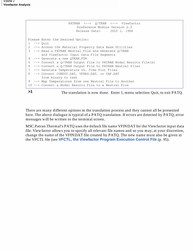
Volume 2Viewfactor Analysis
There are many different options in the translation process and they cannot all be presented here. The above dialogue is typical of a PATQ translation. If errors are detected by PATQ, error messages will be written to the terminal screen.
MSC.Patran Thermal’s PATQ uses the default file name VFINDAT for the Viewfactor input data file. Viewfactor allows you to specify all relevant file names and so you may, at your discretion, change the name of the VFINDAT file created by PATQ. The new name must also be given in the VFCTL file (see VFCTL, the Viewfactor Program Execution Control File (p. 95).
PATRAN <--> Q/TRAN <--> ViewfactorPreference Module Version 2.3Release Date: JULY 1, 1988
Please Enter the Desired Option:1 --> Quit2 --> Access the Material Property Data Base Utilities3 --> Read a PATRAN Neutral File and Generate Q/TRAN and Viewfactor Input Data File Segments4 --> Generate a new QTRAN.FOR5 --> Convert a Q/TRAN Output File to PATRAN Nodal Results File(s)6 --> Convert a Q/TRAN Output File to PATRAN Neutral Files7 --> Generate Temperature vs. Time Plot Files8 --> Convert CONDUC.DAT, VFRES.DAT, or CAP.DAT from binary to text9 --> Map Temperatures from one Neutral File to Another10 --> Convert a Nodal Results File to a Neutral File
>1 The translation is now done. Enter 1, menu selection Quit, to exit PATQ.
9CHAPTER 4Preparation for Analysis
4.4 VFCTL, the Viewfactor Program Execution Control FileThe Viewfactor program execution control file, VFCTL, contains the information needed by Viewfactor to know which parts of the Viewfactor program should be executed, the names of various files needed by Viewfactor and some data or parameters which will influence the viewfactor calculations.
Philosophy and Structure of the VFCTL FileThe VFCTL file is analogous to a session or command file in that it can be thought of as containing commands which set parameters and filenames in the Viewfactor program. This was done because the Viewfactor program will typically be submitted as a batch job or run as a subroutine call. In both cases, the user is not interacting with the program and the run control commands need to be already stored in the VFCTL file.
You may use any nonconflicting legal file name for the VFCTL file. The default name is in the default directory and named VFCTL. A nondefault name must be entered as a parameter on the command line submitting a Viewfactor job (see Analysis (Ch. 5).
The file may contain comment lines and data lines. Comment lines begin with an asterisk. Data lines begin with a keyword, followed by some data (sometimes optional data). The valid keywords are defined in Keywords in the VFCTL File (p. 98). Lines may contain leading blanks.
Default values are provided automatically for all run control data. You do not need to enter data lines if the default is the desired value. The default values are given in Keywords in the VFCTL File (p. 98). The data lines may be placed in any order and only one occurrence of each keyword is allowed. A complete VFCTL file from a VAX/VMS platform is shown below. The filenames have been made generic, but the $PATH is not generic.
Invalid keywords cause a fatal error. This prevents a costly Viewfactor execution with invalid data.
Note: For execution spawned from MSC.Patran Thermal, this file is automatically created based on input data in the MSC.Patran Thermal Analysis Forms.
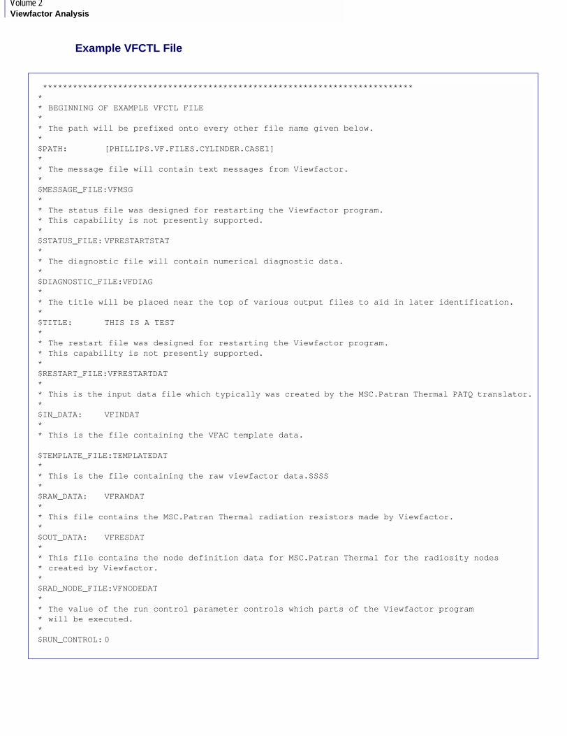
Volume 2Viewfactor Analysis
Example VFCTL File
**************************************************************************** BEGINNING OF EXAMPLE VFCTL FILE** The path will be prefixed onto every other file name given below.*$PATH: [PHILLIPS.VF.FILES.CYLINDER.CASE1]** The message file will contain text messages from Viewfactor.*$MESSAGE_FILE:VFMSG** The status file was designed for restarting the Viewfactor program.* This capability is not presently supported.*$STATUS_FILE: VFRESTARTSTAT** The diagnostic file will contain numerical diagnostic data.*$DIAGNOSTIC_FILE:VFDIAG** The title will be placed near the top of various output files to aid in later identification.*$TITLE: THIS IS A TEST** The restart file was designed for restarting the Viewfactor program.* This capability is not presently supported.*$RESTART_FILE:VFRESTARTDAT** This is the input data file which typically was created by the MSC.Patran Thermal PATQ translator.*$IN_DATA: VFINDAT** This is the file containing the VFAC template data.
$TEMPLATE_FILE:TEMPLATEDAT** This is the file containing the raw viewfactor data.SSSS*$RAW_DATA: VFRAWDAT** This file contains the MSC.Patran Thermal radiation resistors made by Viewfactor.*$OUT_DATA: VFRESDAT** This file contains the node definition data for MSC.Patran Thermal for the radiosity nodes * created by Viewfactor.*$RAD_NODE_FILE:VFNODEDAT** The value of the run control parameter controls which parts of the Viewfactor program* will be executed.*$RUN_CONTROL: 0

9CHAPTER 4Preparation for Analysis
** This parameter controls the restart capabilities of Viewfactor.* Presently only the value 0 is supported (this is not a restart).*$RESTART_FLAG: 0** This parameter controls the convergence checking in Viewfactor. The* value of -1.0 causes a default value based on the number of surfaces* in each enclosure to be calculated.*$CONVERGE -1.0** Viewfactors below the zero cutoff value will be set to 0.0*$ZERO: 0.0** This parameter controls the accuracy of curved surface approximation by * linear surfaces for obstruction checking.*$APPROX_CURVE: 0.1** These values determine the maximum order of numerical integration* quadrature permitted for integration of various quantities.*$GAUSS_ORDER: 8 8 8** These values determine the minimum and maximum number of subdivisions for* the three-dimensional representation of an axisymmetric surface for the* purpose of checking for obstructions and calculating viewfactors.*$AXISYM_SURFACE: 3 13** This keyword signals the end of the VFCTL file.*$EOF:** THIS IS THE END OF THE VFCTL FILE EXAMPLE.***********************************************************************
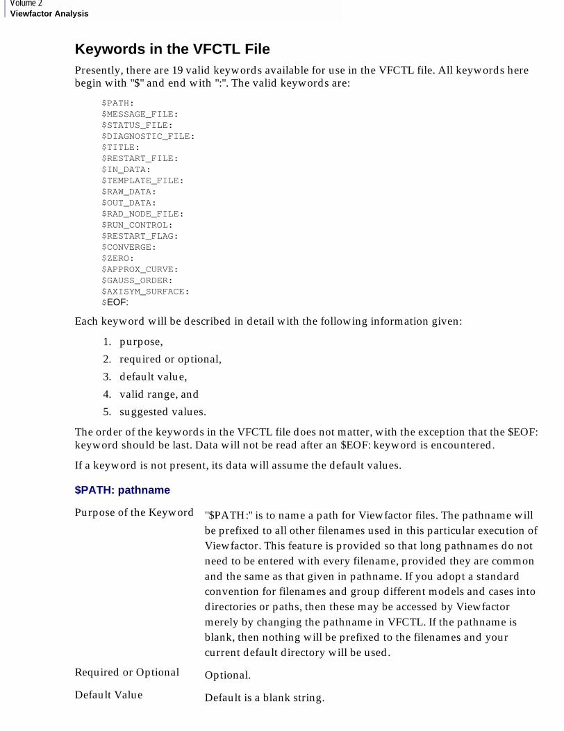
Volume 2Viewfactor Analysis
Keywords in the VFCTL FilePresently, there are 19 valid keywords available for use in the VFCTL file. All keywords here begin with "$" and end with ":". The valid keywords are:
$PATH:$MESSAGE_FILE:$STATUS_FILE:$DIAGNOSTIC_FILE:$TITLE:$RESTART_FILE:$IN_DATA:$TEMPLATE_FILE:$RAW_DATA:$OUT_DATA:$RAD_NODE_FILE:$RUN_CONTROL:$RESTART_FLAG:$CONVERGE:$ZERO:$APPROX_CURVE:$GAUSS_ORDER:$AXISYM_SURFACE:$EOF:
Each keyword will be described in detail with the following information given:
1. purpose,
2. required or optional,
3. default value,
4. valid range, and
5. suggested values.
The order of the keywords in the VFCTL file does not matter, with the exception that the $EOF: keyword should be last. Data will not be read after an $EOF: keyword is encountered.
If a keyword is not present, its data will assume the default values.
$PATH: pathname
Purpose of the Keyword "$PATH:" is to name a path for Viewfactor files. The pathname will be prefixed to all other filenames used in this particular execution of Viewfactor. This feature is provided so that long pathnames do not need to be entered with every filename, provided they are common and the same as that given in pathname. If you adopt a standard convention for filenames and group different models and cases into directories or paths, then these may be accessed by Viewfactor merely by changing the pathname in VFCTL. If the pathname is blank, then nothing will be prefixed to the filenames and your current default directory will be used.
Required or Optional Optional.
Default Value Default is a blank string.
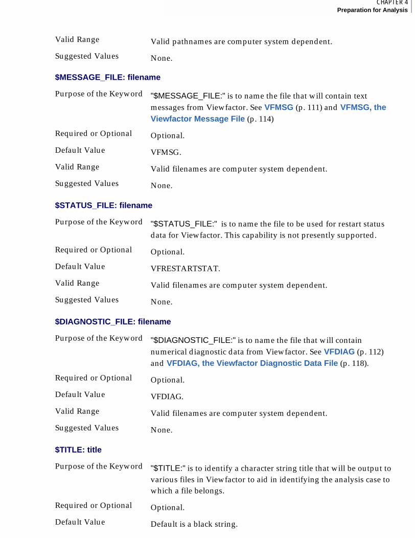
9CHAPTER 4Preparation for Analysis
$MESSAGE_FILE: filename
$STATUS_FILE: filename
$DIAGNOSTIC_FILE: filename
$TITLE: title
Valid Range Valid pathnames are computer system dependent.
Suggested Values None.
Purpose of the Keyword "$MESSAGE_FILE:" is to name the file that will contain text messages from Viewfactor. See VFMSG (p. 111) and VFMSG, the Viewfactor Message File (p. 114)
Required or Optional Optional.
Default Value VFMSG.
Valid Range Valid filenames are computer system dependent.
Suggested Values None.
Purpose of the Keyword "$STATUS_FILE:" is to name the file to be used for restart status data for Viewfactor. This capability is not presently supported.
Required or Optional Optional.
Default Value VFRESTARTSTAT.
Valid Range Valid filenames are computer system dependent.
Suggested Values None.
Purpose of the Keyword "$DIAGNOSTIC_FILE:" is to name the file that will contain numerical diagnostic data from Viewfactor. See VFDIAG (p. 112) and VFDIAG, the Viewfactor Diagnostic Data File (p. 118).
Required or Optional Optional.
Default Value VFDIAG.
Valid Range Valid filenames are computer system dependent.
Suggested Values None.
Purpose of the Keyword "$TITLE:" is to identify a character string title that will be output to various files in Viewfactor to aid in identifying the analysis case to which a file belongs.
Required or Optional Optional.
Default Value Default is a black string.
Volume 2Viewfactor Analysis
$RESTART_FILE: filename
$IN_DATA: filename
$TEMPLATE_FILE: filename
$RAW_DATA: filename
Valid Range The character string should have less than 80 characters.
Suggested Values None.
Purpose of the Keyword "$RESTART"_FILE:" is to name the file that will contain data for restarting Viewfactor. This capability is not presently available.
Required or Optional Optional.
Default Value VFRESTARTDAT.
Valid Range Valid filenames are computer system dependent.
Suggested Values None.
Purpose of the Keyword "$IN_DATA:" is to name the file that must contain the input data for Viewfactor.
Required or Optional Optional.
Default Value VFINDAT.
Valid Range Valid filenames are computer system dependent.
Suggested Values None.
Purpose of the Keyword "$TEMPLATE_FILE:" is to name the file that must contain the VFAC templates for this model.
Required or Optional Optional.
Default Value TEMPLATEDAT.
Valid Range Valid filenames are computer system dependent.
Suggested Values None.
Purpose of the Keyword "$RAW_DATA:" is to name the file which will contain the raw viewfactor data. Viewfactor creates and outputs raw viewfactor data as well as reads in the raw viewfactor data when making MSC.Patran Thermal radiation resistors. See VFRAWDAT (p. 113).
Required or Optional Optional.
Default Value VFRAWDAT.
1CHAPTER 4Preparation for Analysis
$OUT_DATA: filename
$RAD_NODE_FILE: filename
$RUN_CONTROL: value
Valid Range Valid filenames are computer system dependent.
Suggested Values None.
Purpose of the Keyword "$OUT_DATA:" is to name the file which will contain the MSC.Patran Thermal radiation resistor data created by Viewfactor. See VFRESDAT (p. 113).
Required or Optional Optional.
Default Value VFRESDAT.
Valid Range Valid filenames are computer system dependent.
Suggested Values None.
Purpose of the Keyword "$RAD_NODE_FILE:" is to name the file which will contain the node definition data for MSC.Patran Thermal for radiosity nodes created by Viewfactor. See VFNODEDAT (p. 113).
Required or Optional Optional.
Default Value VFNODEDAT.
Valid Range Valid filenames are computer system dependent.
Suggested Values None.
Purpose of the Keyword "$RUN_CONTROL:" is to set a run control value. The run control value determines the execution sequence for Viewfactor. It is this parameter that allows the user to calculate viewfactors before the VFAC templates are ready (set value to 1), calculate or recalculate the MSC.Patran Thermal radiation resistors from existing raw viewfactor data (set value to 2), or calculate viewfactors and make radiation resistors in the same execution (set value to 0). For additional information, see Viewfactor Data and Program Flow (p. 16) and Changing VFCTL (p. 132).
Volume 2Viewfactor Analysis
The valid values of the $RUN_CONTROL: parameter and their effects are:
0 Check data, and if the data checking status = OK, calculate viewfactors and make radiation resistors.
1 Check data, and if the data checking status = OK, calculate viewfactors only.
2 Calculate radiation resistors only, using existing raw viewfactor data. This process involves extensive data checking as the calculations are being done and since no significant CPU time saving is realized, no data checking is done before the calculations.
100 Check the data for making viewfactors and radiation resistors and then stop. Do not calculate viewfactors or make resistors.
101 Check the data for making viewfactors and then stop. Do not calculate viewfactors.
102 Check that the appropriate files are present for making radiation resistors from raw viewfactor data. Do not make the radiation resistors.
200 Check the data for making viewfactors and radiation resistors. If the data checking status = OK or the data only generated warning messages, proceed with the viewfactor calculations and the creation of the radiation resistors. If the data checking generated an error message, stop.
201 Check the data for making viewfactors only. If the data checking status = OK or the data only generated warning messages, proceed with the viewfactor calculations only. If the data checking generated an error message, stop.
202 This option is functionally the same as 2 above.
1000 Skip data checking and proceed directly to calculating the viewfactors and making the radiation resistors.
1001 Skip the data checking and proceed directly to calculating the viewfactors only.
1002 This option is functionally the same as 2 above.
Required or Optional Optional.
1CHAPTER 4Preparation for Analysis
$RESTART_FLAG: value
$CONVERGE: value
Default Value 0.
Valid Range Valid values are the integers listed above.
Suggested Values None.
Purpose of the Keyword "$RESTART_FLAG:" is to set the Viewfactor restart flag. The restart flag value controls restarting Viewfactor. Presently this capability is not supported.
Required or Optional Optional.
Default Value 0.
Valid Range The only valid value is the integer 0.
Suggested Values None.
Purpose of the Keyword "$CONVERGE:" is to set the parameter that controls convergence checking in Viewfactor. If the value entered is less than or equal to zero, a convergence criteria is calculated by Viewfactor based on the number of surfaces in each enclosure. This number will be recalculated as each enclosure is processed. The formula for convergence criteria used by Viewfactor to calculate the default value is:
converge_value = 0.01/(number of surfaces in enclosure)0.7.
Required or Optional Optional.
Default Value -1.0.
Valid Range Valid values are real numbers and representable on the computer.
Suggested Values The suggested value is the default value, -1.0. If a faster execution time is desired, at the cost of lost accuracy, a value around 0.1 may be appropriate. Until you gain some experience with Viewfactor, it is best to use the default value. The convergence criteria is not an absolute requirement. You don’t know how fast the numerical scheme converges. The fact that it appears to have converged over a few iterations is no guarantee that it has converged. The default values are based on previous user's experience. As you gain experience you may be able to improve on these default values.
1.0≤
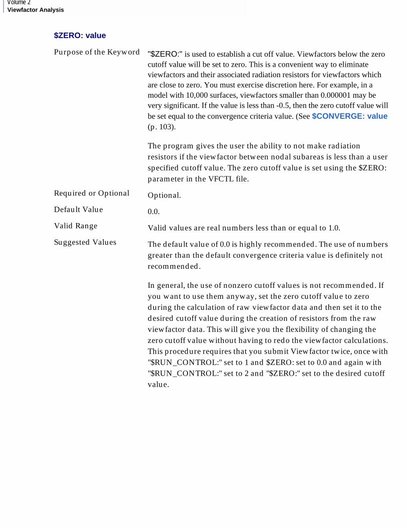
Volume 2Viewfactor Analysis
$ZERO: value
Purpose of the Keyword "$ZERO:" is used to establish a cut off value. Viewfactors below the zero cutoff value will be set to zero. This is a convenient way to eliminate viewfactors and their associated radiation resistors for viewfactors which are close to zero. You must exercise discretion here. For example, in a model with 10,000 surfaces, viewfactors smaller than 0.000001 may be very significant. If the value is less than -0.5, then the zero cutoff value will be set equal to the convergence criteria value. (See $CONVERGE: value (p. 103).
The program gives the user the ability to not make radiation resistors if the viewfactor between nodal subareas is less than a user specified cutoff value. The zero cutoff value is set using the $ZERO: parameter in the VFCTL file.
Required or Optional Optional.
Default Value 0.0.
Valid Range Valid values are real numbers less than or equal to 1.0.
Suggested Values The default value of 0.0 is highly recommended. The use of numbers greater than the default convergence criteria value is definitely not recommended.
In general, the use of nonzero cutoff values is not recommended. If you want to use them anyway, set the zero cutoff value to zero during the calculation of raw viewfactor data and then set it to the desired cutoff value during the creation of resistors from the raw viewfactor data. This will give you the flexibility of changing the zero cutoff value without having to redo the viewfactor calculations. This procedure requires that you submit Viewfactor twice, once with "$RUN_CONTROL:" set to 1 and $ZERO: set to 0.0 and again with "$RUN_CONTROL:" set to 2 and "$ZERO:" set to the desired cutoff value.

1CHAPTER 4Preparation for Analysis
$APPROX_CURVE: value
$GAUSS_ORDER: contours double_area weighting
Purpose of the Keyword "$APPROX_CURVE:" is to set the parameter that controls the number of subdivisions a curved surface or line will undergo as it is approximated by plane triangles or straight line segments. These linear subdivisions are used for obstruction checking. The smaller the value, the more subdivisions will be required to approximate a curved surface or line. As more subdivisions are created, the accuracy of the calculations will generally increase and the CPU time will increase dramatically.
Required or Optional Optional.
Default Value 0.1.
Valid Range Valid values are real numbers less than or equal to 0.5 and greater than or equal to 0.00001 and representable on the computer.
Suggested Values The default value of 0.1 is the recommended value.
Purpose of the Keyword "$GAUSS_ORDER:" is to set the value that will determine the maximum integration order that Viewfactor will attempt to use while trying to satisfy its convergence criteria. The three different values are applied to three different types of integration. Contours applies to contour integration around the border of a surface. Double_area, applies to integration over the surface areas of surface pairs for which partially obstructed viewfactors are being calculated. Weighting, applies to calculations to weight the surface to surface viewfactors according to the finite element interpolation functions.
Note: For straight or planar (flat) surfaces this parameter has little effect since they are already well approximated by linear lines or planes.
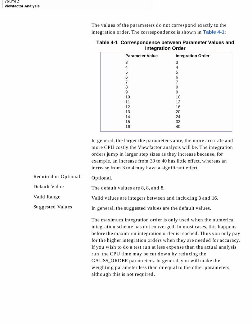
Volume 2Viewfactor Analysis
The values of the parameters do not correspond exactly to the integration order. The correspondence is shown in Table 4-1:
Table 4-1 Correspondence between Parameter Values and Integration Order
In general, the larger the parameter value, the more accurate and more CPU costly the Viewfactor analysis will be. The integration orders jump in larger step sizes as they increase because, for example, an increase from 39 to 40 has little effect, whereas an increase from 3 to 4 may have a significant effect.
Required or Optional Optional.
Default Value The default values are 8, 8, and 8.
Valid Range Valid values are integers between and including 3 and 16.
Suggested Values In general, the suggested values are the default values.
The maximum integration order is only used when the numerical integration scheme has not converged. In most cases, this happens before the maximum integration order is reached. Thus you only pay for the higher integration orders when they are needed for accuracy. If you wish to do a test run at less expense than the actual analysis run, the CPU time may be cut down by reducing the GAUSS_ORDER parameters. In general, you will make the weighting parameter less than or equal to the other parameters, although this is not required.
Parameter Value Integration Order
3 34 45 56 67 78 99 910 1011 1212 1613 2014 2415 3216 40

1CHAPTER 4Preparation for Analysis
$AXISYM_SURFACE: minimum maximum
$EOF:
This concludes the description of the VFCTL keywords.
Purpose of the Keyword "$AXISYM_SURFACE:" is to set the two parameters that control the minimum and maximum number of effective subdivisions the three-dimensional image of an axisymmetric surface is subdivided into for obstruction and viewfactor calculations. Here again, Viewfactor does convergence checking and stops iterating when convergence has occurred. The actual number of subdivisions is not the same as the value of the parameter. They correspond in the same way as the integration orders in Table 4-1.
Required or Optional Optional.
Default Value 3 for the minimum, 13 for the maximum.
Valid Range Valid values are integers , and maximum greater than or equal to minimum.
Suggested Values These parameters have the greatest effect of any of the parameters on the execution time and accuracy of an axisymmetric model submitted for viewfactor calculation. The execution time will increase approximately as the square of the number of subdivisions. Unfortunately, the accuracy does not improve in a like manner. In general, the recommended values are the default values. However, the user may find with some experience that values of maximum as low as 8 give satisfactory results.
Purpose of the Keyword "$EOF:" is to signal the end of the VFCTL file.
Required or Optional Optional.
Default Value,Valid Range,Suggested Values
There is no parameter to receive a default value, be checked for validity, or receive a recommended value.
16 and 3≥≤
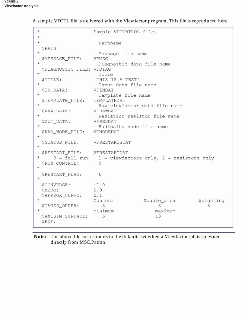
Volume 2Viewfactor Analysis
A sample VFCTL file is delivered with the Viewfactor program. This file is reproduced here.
Note: The above file corresponds to the defaults set when a Viewfactor job is spawned directly from MSC.Patran.
* Sample VFCONTROL file.** Pathname$PATH
* Message file name$MESSAGE_FILE: VFMSG
* Diagnostic data file name$DIAGNOSTIC_FILE: VFDIAG
* Title$TITLE: 'THIS IS A TEST'
* Input data file name$IN_DATA: VFINDAT
* Template file name$TEMPLATE_FILE: TEMPLATEDAT
* Raw viewfactor data file name$RAW_DATA: VFRAWDAT
* Radiation resistor file name$OUT_DATA: VFRESDAT
* Radiosity node file name$RAD_NODE_FILE: VFNODEDAT
*$STATUS_FILE: VFRESTARTSTAT
*$RESTART_FILE: VFRESTARTDAT
* 0 = full run, 1 = viewfactors only, 2 = resistors only$RUN_CONTROL: 0
*$RESTART_FLAG: 0
*$CONVERGE: -1.0$ZERO: 0.0$APPROX_CURVE: 0.1
* Contour Double_area Weighting$GAUSS_ORDER: 8 8 8
* minimum maximum$AXISYM_SURFACE: 5 13$EOF:

MSC.Patran Thermal User’s Guide, Volume 2: Viewfactor Analysis
CHAPTER
5 Analysis
■ Submitting a Viewfactor Job for Analysis
■ Output Created by a Viewfactor Execution
■ Reviewing the Viewfactor Output

Volume 2Viewfactor Analysis
5.1 Submitting a Viewfactor Job for AnalysisSubmitting a Viewfactor job for execution is very simple. Viewfactor analyses take a lot of computer time and real time. Therefore, it is recommended that the model and the VFCTL file be carefully reviewed to double check that the correct data files are present. This will protect you from submitting an analysis with the wrong data and from abnormal execution due to user error.
Review the Viewfactor Control/ParametersYou should review the Viewfactor Solution Parameters in the Analysis form or the VFCTL file being used for this analysis asking the following questions:
1. Is the path name correct?
2. Do all of the input data files exist in the correct directory or will they be automatically created based on the submit options?
3. Are these input data files the correct files for the problem to be analyzed?
The following parameters are described in Keywords in the VFCTL File (p. 98):
1. Does the run control parameter, $RUN_CONTROL:, specify the desired execution sequence?
2. Is the convergence criteria parameter, $CONVERGE:, correct?
3. Is the zero cutoff parameter, $ZERO:, correct?
4. Is the curve approximation parameter, $APPROX_CURVE:, correct?
5. Are the maximum integration order parameters, $GAUSS_ORDER:, correct for
contour integration,double area integration, andfinite element weighting?
6. Are the axisymmetric surface subdivision parameters, $AXISYM_SURFACE:, correct for the
minimum number of subdivisions andmaximum number of subdivisions?
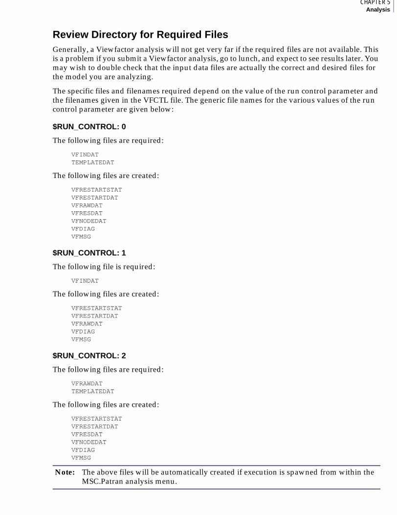
1CHAPTER 5Analysis
Review Directory for Required FilesGenerally, a Viewfactor analysis will not get very far if the required files are not available. This is a problem if you submit a Viewfactor analysis, go to lunch, and expect to see results later. You may wish to double check that the input data files are actually the correct and desired files for the model you are analyzing.
The specific files and filenames required depend on the value of the run control parameter and the filenames given in the VFCTL file. The generic file names for the various values of the run control parameter are given below:
$RUN_CONTROL: 0
The following files are required:
VFINDATTEMPLATEDAT
The following files are created:
VFRESTARTSTATVFRESTARTDATVFRAWDATVFRESDATVFNODEDATVFDIAGVFMSG
$RUN_CONTROL: 1
The following file is required:
VFINDAT
The following files are created:
VFRESTARTSTATVFRESTARTDATVFRAWDATVFDIAGVFMSG
$RUN_CONTROL: 2
The following files are required:
VFRAWDATTEMPLATEDAT
The following files are created:
VFRESTARTSTATVFRESTARTDATVFRESDATVFNODEDATVFDIAGVFMSG
Note: The above files will be automatically created if execution is spawned from within the MSC.Patran analysis menu.
Volume 2Viewfactor Analysis
The Viewfactor Command LineThis section uses examples from a VAX specific installation. Your system may require different commands. Refer to the MSC.Patran Installation and Operations Guide or your system manager.
A Viewfactor analysis is submitted by typing at your computer command prompt the command VSUBMIT followed optionally by the VFCTL filename. The filename must be separated from the command by a comma and/or one or more blank spaces. If no VFCTL file name is given, it will default to VFCTL in the default directory. VSUBMIT may be abbreviated as VSU.
Examples: Let $ be the computer system level prompt. Commands are entered by pressing the RETURN key.
$VSUBMIT Submits a Viewfactor analysis with the VFCTL file from the default directory.
$VSU VFCTL_TEST_RUN Submits a Viewfactor analysis with the control file VFCTL_TEST_RUN from the default directory.
$VSU [SMITH.VF.FILES]VFCONTROL.CON Submits a Viewfactor analysis with the control file VFCONTROL.CON from the directory [PHILLIPS.VF.FILES] on the default disk.
The actual analysis will be run as a batch or background job and you will receive mail or other notification when the job has terminated.
You may also run Viewfactor in interactive mode by using the command VF_RUN instead of VSUBMIT.
Note: A Viewfactor Submit script is automatically created if execution is spawned from within MSC.Patran analysis menu.
1CHAPTER 5Analysis
5.2 Output Created by a Viewfactor ExecutionThe output created by Viewfactor depends on the value of the run control parameter $RUN_CONTROL:. The files VFMSG and VFDIAG are always created (unless a severe error occurs before these files can be opened, which only happens when the file names or directories are invalid). The file VFRAWDAT is created whenever viewfactors are calculated (run control parameter equal 0 or 1). The files VFRESDAT and VFNODEDAT are created whenever MSC.Patran Thermal radiation resistors are made (run control parameter equal 0 or 2). The user’s computer system may also create a log file for the batch or background execution of Viewfactor. Viewfactor will also create VFRESTARTSTAT and VFRESTARTDAT files for its own internal use. These two files will automatically be deleted by Viewfactor before execution terminates. However, if execution is terminated abnormally, these files may be left on the disk and you must delete them.
Examples are shown in Reviewing the Viewfactor Output (p. 114).
VFMSGThis file contains messages from Viewfactor to the user. It begins with a header, followed by the title data from the VFCTL file. Then the control data that was actually used by Viewfactor is echoed to this file. This data may not look quite the same as the user’s VFCTL file. This is because the format may be different and if you allowed any values to default, the default values will be displayed.
The rest of the file contains either informative messages on the progress of the Viewfactor analysis or error messages. Since Viewfactor has been designed to check for many errors and to terminate gracefully on an error condition, the VFMSG file is the only reliable place to find if an error has occurred.
For the most part, Viewfactor will not abort at the computer operating system level. When it detects an error, it reports the error to the VFMSG file and terminates execution without triggering any system level errors. Since there is no system level traceback, the traceback information that Viewfactor outputs to the VFMSG file is very helpful if you need to discuss a problem with MSC’s technical support staff. VFMSG, the Viewfactor Message File (p. 114) contains a sample VFMSG file.
Volume 2Viewfactor Analysis
VFDIAGThis file contains primarily numeric diagnostic data. The file begins with the title data from the VFCTL file, followed by any additional title data from the input data files.
If viewfactors were calculated in this analysis, data is given about the sums of the viewfactors from each surface to every other surface in the enclosure. Similar data is also given for the nodal subareas on each surface.
This data is grouped by enclosure. Each group of enclosure data begins with the keyword $ENCL: followed by the enclosure ID number, the number of surfaces in the enclosure, and the number of symmetric images created of this enclosure. Then for each surface in the enclosure there is a line of data containing the surface ID, the sum of the viewfactors from this surface to all other surfaces in the enclosure, 1.0 minus this sum, and the sum of all viewfactors from this surface to other surfaces which were set to zero because they were less than the zero cutoff value ($ZERO:). Following this line will be the sum of the viewfactors for each nodal subarea on the surface. Thus, there will be the same number of data items as there are nodes on the surface. These data will have four values per line until all of the nodes on this surface are used. Currently, none of the element faces supported by Viewfactor have more than four nodes and hence this data fits on one line. This pattern is repeated for each surface in the enclosure.
After all of the surfaces in the enclosure have been accounted for in the above manner, some statistical data for the enclosure is given. This data is presented in five columns. The first line of statistical data is for the surfaces as wholes and the following lines are statistical data for the nodal subareas of the surfaces. The statistical data for the nodal subareas do not have a sound theoretical basis and should not be taken too seriously. It is, however, the best data available at this time.
The five columns contain the following data:
The data for each enclosure is terminated with the $ENDENCL: keyword. If there is more than one enclosure, the above pattern is repeated for each enclosure.
If MSC.Patran Thermal radiation resistors were created by this execution of Viewfactor, the VFMSG file will contain information on the radiosity nodes, emissivity resistors, and radiation resistors created for each enclosure.
The file is terminated by the keyword $EOF:.
Examples are given in VFDIAG, the Viewfactor Diagnostic Data File (p. 118).
Column 1: The maximum deviation from unity for the sums of viewfactors from a surface or nodal subarea surface to all other surfaces or nodal subarea surfaces in the enclosure.
Column 2: The average deviation from unity for the sums of viewfactors for this enclosure.
Column 3: The standard deviation for the above average.
Column 4: The average of the absolute values of the deviations from unity for the sums of viewfactors in this enclosure.
Column 5: The standard deviation for the above average.
1CHAPTER 5Analysis
VFRAWDATThis is an unformatted (binary) file containing data about the surfaces and raw viewfactor data. Since it is in binary form, the user may not readily examine its contents. The binary form was chosen because this data file tends to be very large and the binary form is considerably more compact than the text form.
VFRESDATThis is also a binary file. It contains data describing the MSC.Patran Thermal radiation resistors. This file is typically very large, hence its binary form. MSC.Patran Thermal can translate the binary form of this file to a text form which the user can read, but it can be a very large file. The procedure for doing this is described in Interface From Viewfactor to MSC.Patran Thermal (p. 123).
This file must be referenced by the MSC.Patran Thermal QINDAT file in order for it to be included in the QTRAN thermal analysis. See Interface From Viewfactor to MSC.Patran Thermal (p. 123).
VFNODEDATThis file contains the information needed by MSC.Patran Thermal to define the additional radiosity nodes created by Viewfactor for the thermal analysis of the thermal radiation interchange. It contains comment lines which begin with a semicolon. If any radiosity nodes were created, the file will contain the line
DEFNOD beginning_node_number ending_node_number 1
for the nodes created by Viewfactor. If no radiosity nodes were created by Viewfactor (all surfaces were black) then the file will contain the comment
;NO ADDITIONAL RADIOSITY NODES WERE GENERATED.
This file must be referenced by the MSC.Patran Thermal QINDAT file in order for it to be included in the QTRAN thermal analysis. See Interface From Viewfactor to MSC.Patran Thermal (p. 123).
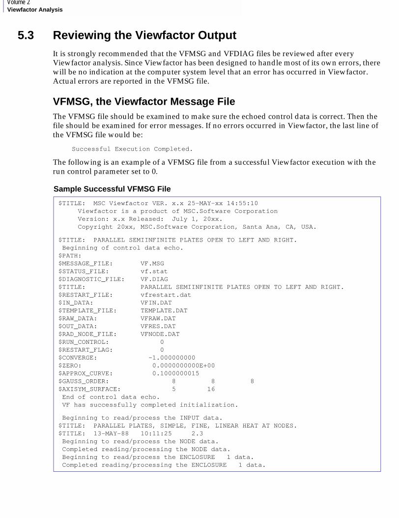
Volume 2Viewfactor Analysis
5.3 Reviewing the Viewfactor OutputIt is strongly recommended that the VFMSG and VFDIAG files be reviewed after every Viewfactor analysis. Since Viewfactor has been designed to handle most of its own errors, there will be no indication at the computer system level that an error has occurred in Viewfactor. Actual errors are reported in the VFMSG file.
VFMSG, the Viewfactor Message FileThe VFMSG file should be examined to make sure the echoed control data is correct. Then the file should be examined for error messages. If no errors occurred in Viewfactor, the last line of the VFMSG file would be:
Successful Execution Completed.
The following is an example of a VFMSG file from a successful Viewfactor execution with the run control parameter set to 0.
Sample Successful VFMSG File
$TITLE: MSC Viewfactor VER. x.x 25-MAY-xx 14:55:10 Viewfactor is a product of MSC.Software Corporation Version: x.x Released: July 1, 20xx. Copyright 20xx, MSC.Software Corporation, Santa Ana, CA, USA.
$TITLE: PARALLEL SEMIINFINITE PLATES OPEN TO LEFT AND RIGHT. Beginning of control data echo.$PATH: $MESSAGE_FILE: VF.MSG$STATUS_FILE: vf.stat$DIAGNOSTIC_FILE: VF.DIAG$TITLE: PARALLEL SEMIINFINITE PLATES OPEN TO LEFT AND RIGHT.$RESTART_FILE: vfrestart.dat$IN_DATA: VFIN.DAT$TEMPLATE_FILE: TEMPLATE.DAT$RAW_DATA: VFRAW.DAT$OUT_DATA: VFRES.DAT$RAD_NODE_FILE: VFNODE.DAT$RUN_CONTROL: 0$RESTART_FLAG: 0$CONVERGE: -1.000000000 $ZERO: 0.0000000000E+00$APPROX_CURVE: 0.1000000015 $GAUSS_ORDER: 8 8 8$AXISYM_SURFACE: 5 16 End of control data echo. VF has successfully completed initialization.
Beginning to read/process the INPUT data.$TITLE: PARALLEL PLATES, SIMPLE, FINE, LINEAR HEAT AT NODES.$TITLE: 13-MAY-88 10:11:25 2.3 Beginning to read/process the NODE data. Completed reading/processing the NODE data. Beginning to read/process the ENCLOSURE 1 data. Completed reading/processing the ENCLOSURE 1 data.
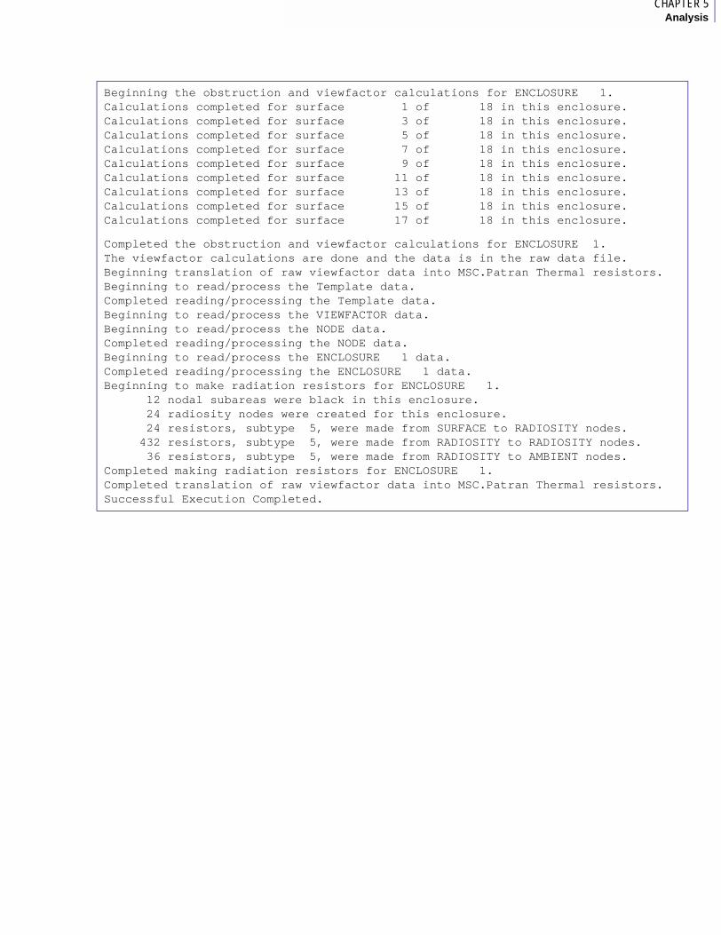
1CHAPTER 5Analysis
Beginning the obstruction and viewfactor calculations for ENCLOSURE 1. Calculations completed for surface 1 of 18 in this enclosure. Calculations completed for surface 3 of 18 in this enclosure. Calculations completed for surface 5 of 18 in this enclosure. Calculations completed for surface 7 of 18 in this enclosure. Calculations completed for surface 9 of 18 in this enclosure. Calculations completed for surface 11 of 18 in this enclosure. Calculations completed for surface 13 of 18 in this enclosure. Calculations completed for surface 15 of 18 in this enclosure. Calculations completed for surface 17 of 18 in this enclosure.
Completed the obstruction and viewfactor calculations for ENCLOSURE 1. The viewfactor calculations are done and the data is in the raw data file. Beginning translation of raw viewfactor data into MSC.Patran Thermal resistors. Beginning to read/process the Template data. Completed reading/processing the Template data. Beginning to read/process the VIEWFACTOR data. Beginning to read/process the NODE data. Completed reading/processing the NODE data. Beginning to read/process the ENCLOSURE 1 data. Completed reading/processing the ENCLOSURE 1 data. Beginning to make radiation resistors for ENCLOSURE 1. 12 nodal subareas were black in this enclosure. 24 radiosity nodes were created for this enclosure. 24 resistors, subtype 5, were made from SURFACE to RADIOSITY nodes. 432 resistors, subtype 5, were made from RADIOSITY to RADIOSITY nodes. 36 resistors, subtype 5, were made from RADIOSITY to AMBIENT nodes. Completed making radiation resistors for ENCLOSURE 1. Completed translation of raw viewfactor data into MSC.Patran Thermal resistors. Successful Execution Completed.
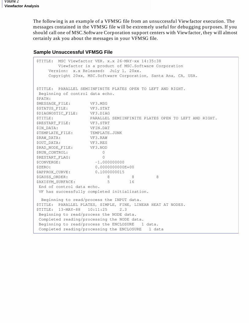
Volume 2Viewfactor Analysis
The following is an example of a VFMSG file from an unsuccessful Viewfactor execution. The messages contained in the VFMSG file will be extremely useful for debugging purposes. If you should call one of MSC.Software Corporation support centers with Viewfactor, they will almost certainly ask you about the messages in your VFMSG file.
Sample Unsuccessful VFMSG File
$TITLE: MSC Viewfactor VER. x.x 26-MAY-xx 14:35:38 Viewfactor is a product of MSC.Software Corporation Version: x.x Released: July 1, 20xx. Copyright 20xx, MSC.Software Corporation, Santa Ana, CA, USA.
$TITLE: PARALLEL SEMIINFINITE PLATES OPEN TO LEFT AND RIGHT. Beginning of control data echo.$PATH: $MESSAGE_FILE: VF3.MSG$STATUS_FILE: VF3.STAT$DIAGNOSTIC_FILE: VF3.DIAG$TITLE: PARALLEL SEMIINFINITE PLATES OPEN TO LEFT AND RIGHT.$RESTART_FILE: VF3.STRT$IN_DATA: VFIN.DAT$TEMPLATE_FILE: TEMPLATE.JUNK$RAW_DATA: VF3.RAW$OUT_DATA: VF3.RES$RAD_NODE_FILE: VF3.NOD$RUN_CONTROL: 0 $RESTART_FLAG: 0$CONVERGE: -1.000000000 $ZERO: 0.0000000000E+00$APPROX_CURVE: 0.1000000015 $GAUSS_ORDER: 8 8 8$AXISYM_SURFACE: 5 16 End of control data echo. VF has successfully completed initialization.
Beginning to read/process the INPUT data.$TITLE: PARALLEL PLATES, SIMPLE, FINE, LINEAR HEAT AT NODES.$TITLE: 13-MAY-88 10:11:25 2.3 Beginning to read/process the NODE data. Completed reading/processing the NODE data. Beginning to read/process the ENCLOSURE 1 data. Completed reading/processing the ENCLOSURE 1 data
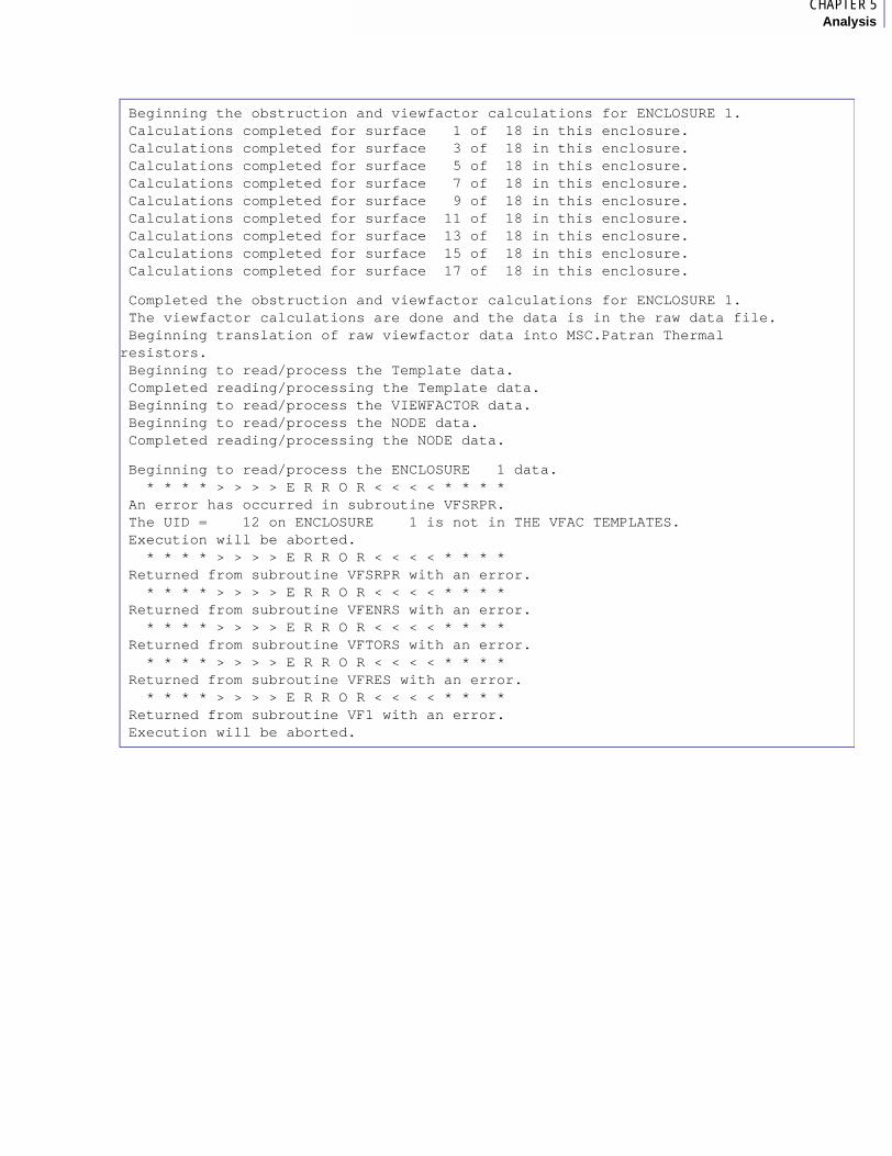
1CHAPTER 5Analysis
Beginning the obstruction and viewfactor calculations for ENCLOSURE 1. Calculations completed for surface 1 of 18 in this enclosure. Calculations completed for surface 3 of 18 in this enclosure. Calculations completed for surface 5 of 18 in this enclosure. Calculations completed for surface 7 of 18 in this enclosure. Calculations completed for surface 9 of 18 in this enclosure. Calculations completed for surface 11 of 18 in this enclosure. Calculations completed for surface 13 of 18 in this enclosure. Calculations completed for surface 15 of 18 in this enclosure. Calculations completed for surface 17 of 18 in this enclosure.
Completed the obstruction and viewfactor calculations for ENCLOSURE 1. The viewfactor calculations are done and the data is in the raw data file. Beginning translation of raw viewfactor data into MSC.Patran Thermal resistors. Beginning to read/process the Template data. Completed reading/processing the Template data. Beginning to read/process the VIEWFACTOR data. Beginning to read/process the NODE data. Completed reading/processing the NODE data.
Beginning to read/process the ENCLOSURE 1 data. * * * * > > > > E R R O R < < < < * * * * An error has occurred in subroutine VFSRPR. The UID = 12 on ENCLOSURE 1 is not in THE VFAC TEMPLATES. Execution will be aborted. * * * * > > > > E R R O R < < < < * * * * Returned from subroutine VFSRPR with an error. * * * * > > > > E R R O R < < < < * * * * Returned from subroutine VFENRS with an error. * * * * > > > > E R R O R < < < < * * * * Returned from subroutine VFTORS with an error. * * * * > > > > E R R O R < < < < * * * * Returned from subroutine VFRES with an error. * * * * > > > > E R R O R < < < < * * * * Returned from subroutine VF1 with an error. Execution will be aborted.
Volume 2Viewfactor Analysis
VFDIAG, the Viewfactor Diagnostic Data FileThe numeric diagnostic data is more difficult to review since there are no simple rules for determining acceptable values.
In general, for a closed enclosure, the sums of the viewfactors should not deviate much from one. How much is too much is left to the discretion of the user and will depend on how many surfaces are in the enclosure, how complicated the obstructions in the enclosure are, and on the VFCTL parameters for convergence and integration order $CONVERGE:, $GAUSS_ORDER:, and $AXISYM_SURFACE:.
For an enclosure with symmetric images, if the object with its symmetric images is closed, then sums of viewfactors significantly greater than one indicate that too many symmetric images were created. If the sums are significantly less than one, then this may indicate that not enough symmetric images were created. Here a significant deviation from one is on the order of the inverse of the number of symmetric images.
If the enclosure is open, the sums for surfaces which have a view of the opening should be somewhat less than one. In some simple geometries, you may be able to calculate the view of the opening for some of the surfaces. This number may be compared with the value of one minus the sum for a very good test of the accuracy of the viewfactor analysis.
For larger problems, the statistical information at the end of each enclosure in the VFDIAG file provides a convenient summary of the diagnostic data for that enclosure. The nature of this data was explained in VFDIAG (p. 112). Your own discretion must be used when evaluating this data.
If you deem the accuracy of the analysis to be inadequate, then this may be remedied by increasing the maximum integration order, reducing the convergence criteria, and refining the finite element mesh in the model. Unfortunately, there are no guarantees here and no one particular method can be counted on to work in every situation.
The following is an example of a VFDIAG file. The enclosure here is the interior of a hollow cube. The faces were modeled with a very coarse mesh and have both triangular and quadrilateral faces. There are 9 surfaces in the model. Since this is a closed enclosure, we expect the sums of the viewfactors should be very close to one. The diagnostic data indicates that for the surfaces the sums are very close to one. However, the sums for the nodal subareas tend to deviate from one by several percent.
You might reduce this error by increasing the integration order, decreasing the convergence criteria, or refining the coarse mesh in the model.
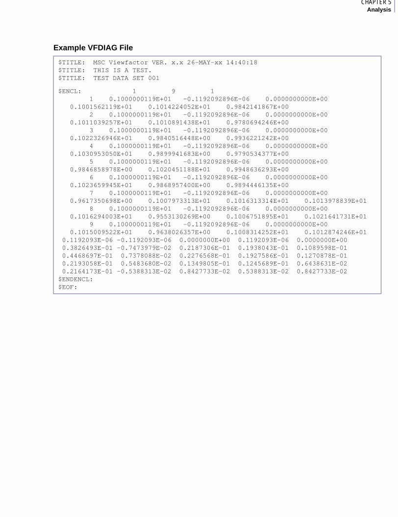
1CHAPTER 5Analysis
Example VFDIAG File
$TITLE: MSC Viewfactor VER. x.x 26-MAY-xx 14:40:18 $TITLE: THIS IS A TEST.$TITLE: TEST DATA SET 001
$ENCL: 1 9 1 1 0.1000000119E+01 -0.1192092896E-06 0.0000000000E+00 0.1001562119E+01 0.1014224052E+01 0.9842141867E+00 2 0.1000000119E+01 -0.1192092896E-06 0.0000000000E+00 0.1011039257E+01 0.1010891438E+01 0.9780694246E+00 3 0.1000000119E+01 -0.1192092896E-06 0.0000000000E+00 0.1022326946E+01 0.9840516448E+00 0.9936221242E+00 4 0.1000000119E+01 -0.1192092896E-06 0.0000000000E+00 0.1030953050E+01 0.9899941683E+00 0.9790534377E+00 5 0.1000000119E+01 -0.1192092896E-06 0.0000000000E+00 0.9846858978E+00 0.1020451188E+01 0.9948636293E+00 6 0.1000000119E+01 -0.1192092896E-06 0.0000000000E+00 0.1023659945E+01 0.9868957400E+00 0.9894446135E+00 7 0.1000000119E+01 -0.1192092896E-06 0.0000000000E+00 0.9617350698E+00 0.1007973313E+01 0.1016313314E+01 0.1013978839E+01 8 0.1000000119E+01 -0.1192092896E-06 0.0000000000E+00 0.1016294003E+01 0.9553130269E+00 0.1006751895E+01 0.1021641731E+01 9 0.1000000119E+01 -0.1192092896E-06 0.0000000000E+00 0.1015009522E+01 0.9638026357E+00 0.1008314252E+01 0.1012874246E+01 0.1192093E-06 -0.1192093E-06 0.0000000E+00 0.1192093E-06 0.0000000E+00 0.3826493E-01 -0.7473979E-02 0.2187306E-01 0.1938043E-01 0.1089598E-01 0.4468697E-01 0.7378088E-02 0.2276568E-01 0.1927586E-01 0.1270878E-01 0.2193058E-01 0.5483680E-02 0.1349805E-01 0.1245689E-01 0.6438631E-02 0.2164173E-01 -0.5388313E-02 0.8427733E-02 0.5388313E-02 0.8427733E-02$ENDENCL:$EOF:

Volume 2Viewfactor Analysis
MSC.Patran Thermal User’s Guide, Volume 2: Viewfactor Analysis
CHAPTER
6 Post-Analysis
■ Introduction
■ Interface From Viewfactor to MSC.Patran Thermal
■ Notes on Resistor Values
■ THERMAL Analysis
■ THERMAL Results Postprocessing

Volume 2Viewfactor Analysis
6.1 IntroductionPost-analysis, includes the activities that normally follow a Viewfactor analysis. These activities primarily involve interfacing to MSC.Patran Thermal for subsequent thermal network analysis. This chapter assumes that you have used Viewfactor to create MSC.Patran Thermal radiation resistors and now want to include them in a thermal analysis.
Viewfactor may also be used to calculate viewfactors only and not make MSC.Patran Thermal radiation resistors, or be used to take already existing viewfactor data and combine it with MSC.Patran Thermal template file data to produce radiation resistors. These different modes of operation are determined by the $RUN_CONTROL parameter.
For more information on these different modes of operation, see Description (p. 14), VFCTL, the Viewfactor Program Execution Control File (p. 95), Review Directory for Required Files (p. 109) and Changing the Surface Template Data After Viewfactors are Calculated (Ch. 7).
1CHAPTER 6Post-Analysis
6.2 Interface From Viewfactor to MSC.Patran ThermalThere are two possible interfaces for the Viewfactor results in the form of the radiative resistors in the VFRESDAT file and the radiosity nodes in the VFNODEDAT file to the MSC.Patran Thermal analysis module. The first of these is the use of the data as input to the thermal network analysis code QTRAN and the second is through a translator in PATQ to change the binary form of the radiative resistor file to text form readable by the user. Refer to the MSC.Patran Thermal User’s Guide, Volume 1: Thermal/Hydraulic Analysis for more information on PATQ and QTRAN.
Viewfactor VFRESDAT and VFNODEDAT Files as Input to MSC.Patran Thermal’s QTRANTo include the thermal radiation network data from Viewfactor in the MSC.Patran Thermal analysis by QTRAN, the user must include the two files from Viewfactor (VFRESDAT and VFNODEDAT) in the QINDAT file for QTRAN. This is typically done by using QTRAN’s $INSERT command in the QINDAT file.
If you are not using the standard filenames, then you need to substitute the filenames in use at the time.
The VFNODEDAT file should be included in the QTRAN QINDAT. See VFNODEDAT (p. 113). This is done with the line
$INSERT VFNODEDAT
This line must be in the QINDAT DEFNOD section, that is before the $ sign terminating the section and typically after the $INSERT NODEDAT line.
The VFRESDAT radiation resistor data file should be included in the QTRAN QINDAT, VFMSG, the Viewfactor Message File (p. 114): RESISTOR DATA SETS of the QINDAT file. This is done with the line
$INSERT VFRESDAT,RAD
A sample QINDAT file is shown with the parts relevant to the Viewfactor files VFRESDAT and VFNODEDAT shown in bold. This example was created on a VAX VMS computer platform. If you have a different platform, see your MSC.Patran Thermal User’s Guide, Volume 1: Thermal/Hydraulic Analysis for the system dependent file names.
Note: The following steps are automatically handled if execution is spawned from within the MSC.Patran analysis form.
Note: The QINDAT file is automatically created when execution is spawned from MSC.Patran and is described in the MSC.Patran Thermal User’s Guide, Volume 1: Thermal/Hydraulic Analysis.
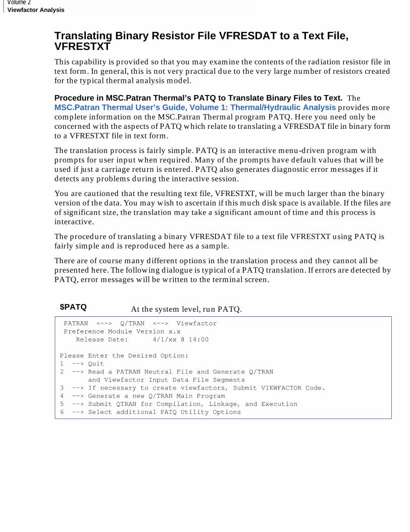
Volume 2Viewfactor Analysis
Translating Binary Resistor File VFRESDAT to a Text File, VFRESTXTThis capability is provided so that you may examine the contents of the radiation resistor file in text form. In general, this is not very practical due to the very large number of resistors created for the typical thermal analysis model.
Procedure in MSC.Patran Thermal’s PATQ to Translate Binary Files to Text. The MSC.Patran Thermal User’s Guide, Volume 1: Thermal/Hydraulic Analysis provides more complete information on the MSC.Patran Thermal program PATQ. Here you need only be concerned with the aspects of PATQ which relate to translating a VFRESDAT file in binary form to a VFRESTXT file in text form.
The translation process is fairly simple. PATQ is an interactive menu-driven program with prompts for user input when required. Many of the prompts have default values that will be used if just a carriage return is entered. PATQ also generates diagnostic error messages if it detects any problems during the interactive session.
You are cautioned that the resulting text file, VFRESTXT, will be much larger than the binary version of the data. You may wish to ascertain if this much disk space is available. If the files are of significant size, the translation may take a significant amount of time and this process is interactive.
The procedure of translating a binary VFRESDAT file to a text file VFRESTXT using PATQ is fairly simple and is reproduced here as a sample.
There are of course many different options in the translation process and they cannot all be presented here. The following dialogue is typical of a PATQ translation. If errors are detected by PATQ, error messages will be written to the terminal screen.
$PATQ At the system level, run PATQ.
PATRAN <--> Q/TRAN <--> Viewfactor Preference Module Version x.x Release Date: 4/1/xx @ 14:00
Please Enter the Desired Option:1 --> Quit2 --> Read a PATRAN Neutral File and Generate Q/TRAN and Viewfactor Input Data File Segments3 --> If necessary to create viewfactors, Submit VIEWFACTOR Code.4 --> Generate a new Q/TRAN Main Program5 --> Submit QTRAN for Compilation, Linkage, and Execution6 --> Select additional PATQ Utility Options
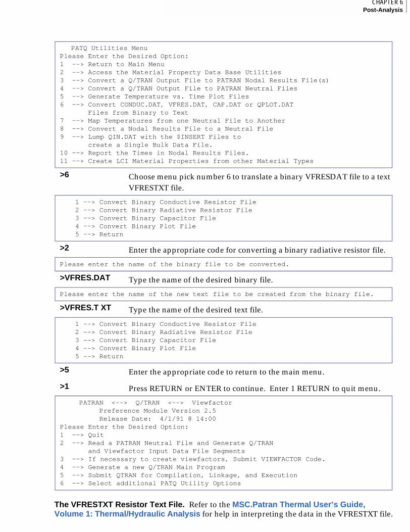
1CHAPTER 6Post-Analysis
The VFRESTXT Resistor Text File. Refer to the MSC.Patran Thermal User’s Guide, Volume 1: Thermal/Hydraulic Analysis for help in interpreting the data in the VFRESTXT file.
PATQ Utilities MenuPlease Enter the Desired Option:1 --> Return to Main Menu2 --> Access the Material Property Data Base Utilities3 --> Convert a Q/TRAN Output File to PATRAN Nodal Results File(s)4 --> Convert a Q/TRAN Output File to PATRAN Neutral Files5 --> Generate Temperature vs. Time Plot Files6 --> Convert CONDUC.DAT, VFRES.DAT, CAP.DAT or QPLOT.DAT Files from Binary to Text7 --> Map Temperatures from one Neutral File to Another8 --> Convert a Nodal Results File to a Neutral File9 --> Lump QIN.DAT with the $INSERT Files to create a Single Bulk Data File.10 --> Report the Times in Nodal Results Files.11 --> Create LCI Material Properties from other Material Types
>6 Choose menu pick number 6 to translate a binary VFRESDAT file to a text VFRESTXT file.
1 --> Convert Binary Conductive Resistor File 2 --> Convert Binary Radiative Resistor File 3 --> Convert Binary Capacitor File 4 --> Convert Binary Plot File 5 --> Return
>2 Enter the appropriate code for converting a binary radiative resistor file.
Please enter the name of the binary file to be converted.
>VFRES.DAT Type the name of the desired binary file.
Please enter the name of the new text file to be created from the binary file.
>VFRES.T XT Type the name of the desired text file.
1 --> Convert Binary Conductive Resistor File 2 --> Convert Binary Radiative Resistor File 3 --> Convert Binary Capacitor File 4 --> Convert Binary Plot File 5 --> Return
>5 Enter the appropriate code to return to the main menu.
>1 Press RETURN or ENTER to continue. Enter 1 RETURN to quit menu.
PATRAN <--> Q/TRAN <--> Viewfactor Preference Module Version 2.5 Release Date: 4/1/91 @ 14:00Please Enter the Desired Option:1 --> Quit2 --> Read a PATRAN Neutral File and Generate Q/TRAN and Viewfactor Input Data File Segments3 --> If necessary to create viewfactors, Submit VIEWFACTOR Code.4 --> Generate a new Q/TRAN Main Program5 --> Submit QTRAN for Compilation, Linkage, and Execution6 --> Select additional PATQ Utility Options

Volume 2Viewfactor Analysis
6.3 Notes on Resistor ValuesWhen Viewfactor makes resistors from a surface to the ambient environment node, it calculates the view to the ambient environment by summing the viewfactors from the surface to all other surfaces in the enclosure and subtracting from one. If the opening in the enclosure is small, it is possible to obtain a small negative number by this procedure due to numerical and round-off error. This will result in a resistor with a negative value. This is not a problem for the network analyzer QTRAN and you should not become unduly alarmed about these negative valued resistors. They are retained because they are the best approximation of the correct value.
1CHAPTER 6Post-Analysis
6.4 THERMAL AnalysisThermal analysis is covered in detail in the MSC.Patran Thermal User’s Guide, Volume 1: Thermal/Hydraulic Analysis. You are referred there for a complete discussion of thermal analysis using the MSC.Patran Plus family of products.
The basic procedure is to enter the PATQ program and choose menu pick number 4, Generate a new QTRANFOR. After exiting PATQ, you submit the thermal analysis for compilation, linking, and execution by the MSC.Patran Thermal command QTRAN. Status and progress of the thermal analysis may be monitored using the MSC.Patran Thermal command QS.
Note: These commands are computer system dependent. They are the standard commands on a VAX/VMS system. If you have a different system or have customized your installation, then your commands may be different. Refer to the MSC.Patran Thermal User’s Guide, Volume 1: Thermal/Hydraulic Analysis or your system manager.

Volume 2Viewfactor Analysis
6.5 THERMAL Results PostprocessingPostprocessing the thermal analysis results is described in detail in the MSC.Patran Thermal User’s Guide and postprocessing in general is described in the MSC.Patran Reference Manual.
Basically, MSC.Patran Thermal will produce MSC.Patran nodal results or neutral files for use by MSC.Patran. You should note that the radiosity nodes, being nonphysical, are not part of the MSC.Patran geometric model and hence these nodes and the results at these nodes cannot easily be displayed in MSC.Patran Plus. The results at these nodes may be examined in the QOUTDAT file. Also, the QOUTDAT file has additional information on the radiation resistors and the heat flow through these resistors which you may wish to examine. The QOUTDAT file is documented in the MSC.Patran Thermal User’s Guide.
MSC.Patran Thermal User’s Guide, Volume 2: Viewfactor Analysis
CHAPTER
7 Changing the Surface Template Data After Viewfactors are Calculated
■ Introduction
■ Compatible VFAC LBC and Template Data
■ New Resistors from Raw Viewfactor Data

Volume 2Viewfactor Analysis
7.1 IntroductionViewfactor has been carefully designed to segregate the viewfactor calculations (which depend only on the geometry of the model and are completely independent of the material properties) from that part of the program which creates the MSC.Patran Thermal radiation resistors (by combining the viewfactors and material property data). This gives you the luxury of calculating the viewfactors once for a given model. Then if you change materials or material properties, you can get the new MSC.Patran Thermal radiation resistors without having to recalculate the viewfactors. The viewfactor calculations typically take a lot of computer time. This capability provides a large saving in computer time for models in which the radiative material properties are modeled for various levels of sophistication or for models in which various materials or surface properties are being evaluated.

1CHAPTER 7Changing the Surface Template Data After Viewfactors are Calculated
7.2 Compatible VFAC LBC and Template DataThere are certain compatibility requirements for the VFAC boundary condition and VFAC templates. These requirements are discussed in detail in Compatibility Requirements for Model and VFAC Templates (p. 75). If you plan to change the material properties and make new MSC.Patran Thermal radiation resistors without having to recalculate the viewfactors, it is especially important that these compatibility requirements be satisfied for all of the material properties to be used, and that the VFAC boundary condition data do not need to be changed to model the various materials.

Volume 2Viewfactor Analysis
7.3 New Resistors from Raw Viewfactor Data New and different MSC.Patran Thermal radiation resistors may be created by changing the MSC.Patran Thermal material property definitions in the VFAC templates and in the material property data files where the MPIDs are defined, typically in the MSC.Patran Thermal file MATDAT.
If the VFAC templates are changed, then Viewfactor must be used to create new MSC.Patran Thermal radiation resistors and radiosity nodes.
If the VFAC templates are not changed and only the MSC.Patran Thermal material property definitions are changed (but not the MPIDs), then you do not need to recreate the MSC.Patran Thermal radiation resistors and radiosity nodes. This is because Viewfactor only uses the VFAC templates and the raw viewfactor data to create the MSC.Patran Thermal radiation resistors and radiosity nodes. If the templates and viewfactors are not changed, the resistor will not change.
Changing TEMPLATEDAT VFAC TemplatesChanges in the VFAC templates are typically entered from a text editor. The VFAC templates are described more fully in Relationship of VFAC LBC Data to VFINDAT File Data (p. 59) and in the MSC.Patran Thermal User’s Guide.
If the VFAC templates are changed, then Viewfactor must be rerun to recreate the MSC.Patran Thermal radiation resistors and radiosity nodes.
Note that when you change the VFAC templates you need not recalculate the viewfactors. You only need to recreate the resistor data. Instructions for running Viewfactor in this mode are given in Compatible VFAC LBC and Template Data (p. 131).
Once again, remember the compatibility requirements for VFAC LBCs and VFAC templates referred to in the previous section and MSC.Patran Thermal TEMPLATEDAT Files for Surface Property Description (p. 60).
Changing MSC.Patran Thermal Material DefinitionsThe material property definitions are part of MSC.Patran Thermal. Refer to the MSC.Patran Thermal User’s Guide for more information. As long as the material property ID, MPID, and VFAC template are not changed, the existing MSC.Patran Thermal radiation resistors and radiosity nodes will be valid. This allows for wide latitude in material properties, provided compatibility was insured when the model was created. For example, a material property which was originally modeled as a constant in its MPID definition may be changed to a temperature dependent function merely by changing it's MPID definition in the MSC.Patran Thermal MATDAT file. No changes need to be made to the radiative resistors or radiosity nodes.
Changing VFCTLIf you wish to recreate MSC.Patran Thermal radiation resistors and radiosity nodes and not recalculate the viewfactors, then the run control parameter, $RUN_CONTROL:, in the VFCTL file must be set to the value 2.
Submitting the New Viewfactor JobAll Viewfactor jobs are submitted in the same manner. Refer to Submitting a Viewfactor Job for Analysis (p. 108) for detailed instructions on submitting the Viewfactor job to recreate the MSC.Patran Thermal radiation resistors and radiosity nodes.
MSC.Patran Thermal User’s Guide, Volume 2: Viewfactor Analysis
CHAPTER
8 Theory and Computational Limitations
■ Introduction
■ Viewfactor
■ Mean Beam Length
■ Obstructions
■ Computational Limitations

Volume 2Viewfactor Analysis
8.1 IntroductionThe present Viewfactor program makes commercially available advances in the computer calculation of viewfactors and obstruction for finite element thermal models developed at MSC.Software Corporation. These advances are principally:
1. Improved performance as measured by the product of speed and accuracy in determining obstructed views and calculating viewfactors, and
2. A viewfactor analysis program designed specifically for finite element modeling.

1CHAPTER 8Theory and Computational Limitations
8.2 ViewfactorThe finite element model for the viewfactor associated with the ith node on surface e to the jth node on surface f is represented by the following formula:
Eq. 8-1
subject to the restrictions that does not intersect any view obstructing surfaces and the product is negative, and
where:
The right-hand side of this equation is evaluated using numerical methods. The numerical integration scheme is predominantly Gaussian quadrature. The quadrature order may be varied by the Viewfactor analysis program in an attempt to obtain the desired accuracy. The method for estimating the accuracy of the numerical integration is, of course, empirical, but seems to work very well. In general, if sufficient accuracy has not been obtained, then the quadrature order will be increased in an effort to improve the accuracy. The quadrature order is not increased globally throughout the integration domain, but only in those areas where the program determines the most benefit will result.
e = Surface e ID
f = Surface f ID
i = Node ID on surface e
j = Node ID on surface f
Ae = Surface e area
Af = Surface f area
=Primary variable finite element interpolation function associated with the ith node on surface e
= Vector from a point on surface e to a point on surface f
= Unit normal to surface e
= Magnitude of a vector
Fijef Ae Af
Nie Ni
f ref n̂e•( ) ref n̂f•( )dAedAf
π ref 4----------------------------------------------------------------------------------------------------------∫∫∫∫
eNi
e dAe
∫∫
------------------------------------------------------------------------------------------------------------------------------------------------–=
ref
ref n̂e•( ) ref n̂ f•( )
Nie
ref
n̂e

Volume 2Viewfactor Analysis
8.3 Mean Beam LengthFor the enclosure with an isothermal participating medium (in equilibrium with itself), we may define a quantity analogous to the viewfactor above, called the exchange factor, by the equation:
Eq. 8-2
subject to the restrictions that does not intersect any view obstructing surfaces and the product is negative, and
where:
For the optically thin media, the exponential function in the above equation may be approximated by:
Eq. 8-3
Using this approximation and assuming that the extinction coefficient is constant (or close enough to constant that it may be taken outside the integration), define the mean beam length by the equation:
Eq. 8-4
Then in MSC.Patran Thermal the exchange factor is approximated by the equation:
e = Surface e ID
f = Surface f ID
i = Node ID on surface e
j = Node ID on surface f
Ae = Surface e area
Af = Surface f area
k media extinction coefficient
=Primary variable finite element interpolation function associated with the ith node on surface e
= Vector from a point on surface e to a point on surface f
= Unit normal to surface e
= Magnitude of a vector
Io ijef Ae Af
exp κ ref–( )Nie Nif ref n̂e•( ) ref n̂f•( )dAedAf
π ref 4----------------------------------------------------------------------------------------------------------------------------------------∫∫∫∫
eNi
e dAe
∫∫
-----------------------------------------------------------------------------------------------------------------------------------------------------------------------------–=
ref
ref n̂e•( ) ref n̂ f•( )
Nie
ref
n̂e
exp κ ref–( ) 1 κ ref– higher order terms+=
Ri jef Ae Af
Nie Ni
f ref n̂e•( ) ref n̂f•( )dAedAf
π ref 3----------------------------------------------------------------------------------------------------------∫∫∫∫
eNi
e dAe
∫∫
------------------------------------------------------------------------------------------------------------------------------------------------–=

1CHAPTER 8Theory and Computational Limitations
Eq. 8-5
In this way the geometry of the model is isolated in the viewfactor and mean beam length quantities. The material properties, such as the extinction coefficient, may be time and temperature dependent functions in MSC.Patran Thermal without requiring recalculation of the viewfactor and mean beam length. This results in great saving of computer processing time.
The assumptions made for the participating media model in Viewfactor and MSC.Patran Thermal are as follows:
1. The media is isothermal;
2. The media is in equilibrium with its internal energy;
3. The media extinction coefficient is not a function of position;
4. The optical thickness is small enough that the linear approximation of the exponential function is reasonable and the media is only weakly interacting with itself.
Io ijef exp κ Rij
ef–( )Fijef=

Volume 2Viewfactor Analysis
8.4 ObstructionsIt is understood that the finite element discretization of the model geometry represents the finest geometric detail available in the model. Therefore, surfaces are not subdivided beyond the nodal subareas for obstruction checking. This restriction on obstruction checking may be viewed as a bit too severe. Different schemes have been tried. The error introduced by this discretization of the obstruction checking process was compared with the error introduced in the viewfactors by the finite element discretization. Considering the cost in computer execution time for a finer obstruction discretization, it was better to limit the obstruction checking to nodal subareas.
You have control over the accuracy of the obstruction test in the usual way that accuracy in a finite element model is controlled (i. e., by refining the finite element mesh). Thus, if more accuracy is needed in the obstruction checking, you should refine the finite element mesh in the regions where greater accuracy is desired.
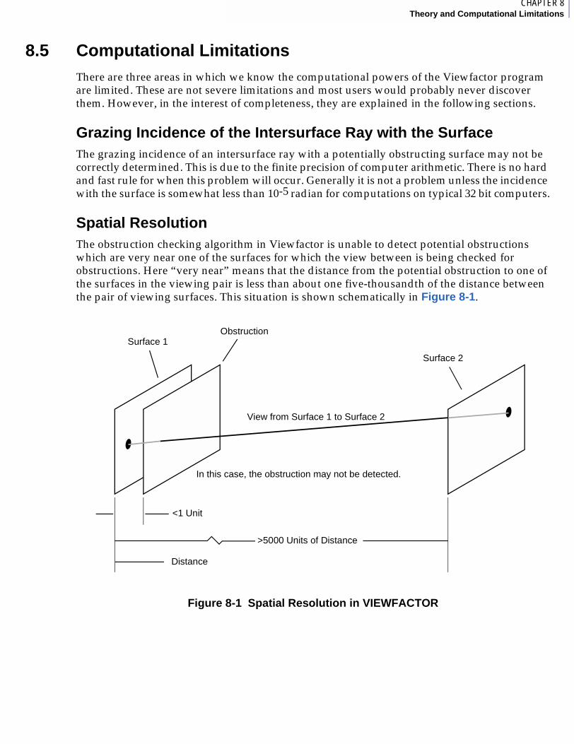
1CHAPTER 8Theory and Computational Limitations
8.5 Computational LimitationsThere are three areas in which we know the computational powers of the Viewfactor program are limited. These are not severe limitations and most users would probably never discover them. However, in the interest of completeness, they are explained in the following sections.
Grazing Incidence of the Intersurface Ray with the SurfaceThe grazing incidence of an intersurface ray with a potentially obstructing surface may not be correctly determined. This is due to the finite precision of computer arithmetic. There is no hard and fast rule for when this problem will occur. Generally it is not a problem unless the incidence with the surface is somewhat less than 10-5 radian for computations on typical 32 bit computers.
Spatial ResolutionThe obstruction checking algorithm in Viewfactor is unable to detect potential obstructions which are very near one of the surfaces for which the view between is being checked for obstructions. Here “very near” means that the distance from the potential obstruction to one of the surfaces in the viewing pair is less than about one five-thousandth of the distance between the pair of viewing surfaces. This situation is shown schematically in Figure 8-1.
Figure 8-1 Spatial Resolution in VIEWFACTOR
Surface 1Obstruction
Surface 2
View from Surface 1 to Surface 2
In this case, the obstruction may not be detected.
<1 Unit
Distance
>5000 Units of Distance

Volume 2Viewfactor Analysis
Extreme ScalesModels which have very large or very small numbers for their dimensions will cause an arithmetic overflow or underflow condition to occur in Viewfactor. The approximate limits at which this occurs depends on the dimensionality of the model. For the 2-D XY model, the limits are approximately the square root of the largest and smallest numbers representable in the default FORTRAN single precision variable. For the 2-D RZ axisymmetric model, these limits are approximately the cube root of the largest and smallest numbers representable in the default FORTRAN single precision variable. For the 3-D XYZ model, these limits are approximately the fourth root of the largest and smallest numbers representable in the default FORTRAN single precision variable. If the user’s model has dimensions which exceed these upper or lower limits it will be necessary to scale the model by a suitable factor in order to avoid arithmetic overflow or underflow in Viewfactor. Viewfactor does not check for overflow and underflow conditions, since for most users this will not be an issue.
MSC.Patran Thermal User’s Guide, Volume 2: Viewfactor Analysis
CHAPTER
9 Data File Specifications
■ Introduction
■ VFINDAT (Input Data File)
■ VFRAWDAT (Raw Viewfactor Data)
■ VFRESDAT (Resistor Data)
■ VFDIAG (Diagnostic Data)
■ TEMPLATEDAT (Surface Pointer Data)
■ VFNODEDAT (Radiosity Node Lists)

Volume 2Viewfactor Analysis
9.1 IntroductionA computer programmer may wish to write an interface to the Viewfactor data files. These data file specifications are intended to provide the information necessary. Unless you wish to examine the contents of these files, you don’t need to be concerned with this chapter.

1CHAPTER 9Data File Specifications
9.2 VFINDAT (Input Data File)This file contains the data describing the model for which viewfactors are to be calculated. It is identified by the $IN_FILE: keyword in the Viewfactor command file. Its default name is VFINDAT. This file is currently a sequential, formatted (ascii) file. We may optionally provide this file in sequential, unformatted (binary) form sometime in the future to better accommodate large models.
The file contains comments, keyword lines, and numeric data.
Comments are blank lines or lines where the first nonblank character is *. Comments may not immediately precede or be interspersed with numeric data. Comments may immediately precede any keyword line.
Keyword lines consist of a keyword which may be followed by data as described in more detail below. All keyword lines are required and must be in the order shown. The number of occurrences permitted for different keywords is described in more detail below. The valid keywords and order are:
$TITLE:$SIZE:$SYM:$ENDSYM:$NODES:$ENDNODES:$ENCL:$ENDENCL:$EOF:
Leading blanks may precede comments and keywords. Comments and keyword lines are read by a FORTRAN '(A)' format into a buffer 132 characters long. Thus, comments and keyword lines (including leading blanks) should not exceed 132 characters.
Numeric data is associated with keywords and may occur on the keyword line or on line(s) immediately following the keyword line. Note that comments are not permitted immediately preceding or interspersed with numeric data. Numeric data is in a fixed format which will be described in detail (see Examples (p. 144)).
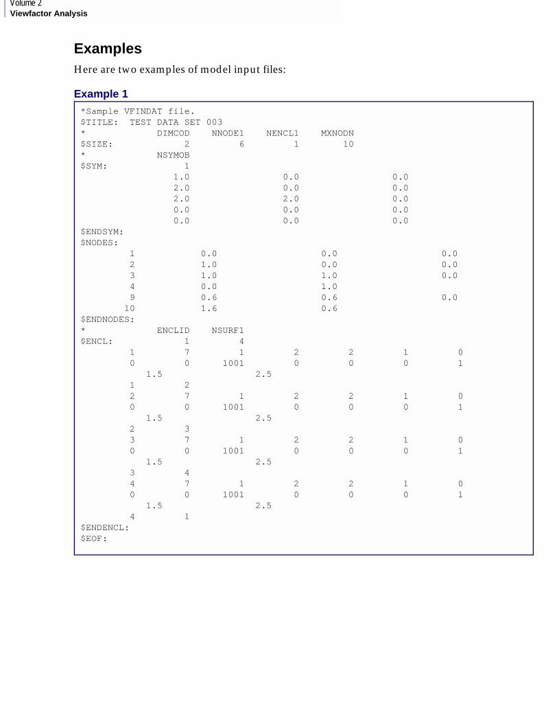
Volume 2Viewfactor Analysis
ExamplesHere are two examples of model input files:
Example 1*Sample VFINDAT file.$TITLE: TEST DATA SET 003* DIMCOD NNODE1 NENCL1 MXNODN$SIZE: 2 6 1 10* NSYMOB$SYM: 1 1.0 0.0 0.0 2.0 0.0 0.0 2.0 2.0 0.0 0.0 0.0 0.0 0.0 0.0 0.0$ENDSYM:$NODES: 1 0.0 0.0 0.0 2 1.0 0.0 0.0 3 1.0 1.0 0.0 4 0.0 1.0 9 0.6 0.6 0.0 10 1.6 0.6$ENDNODES:* ENCLID NSURF1$ENCL: 1 4 1 7 1 2 2 1 0 0 0 1001 0 0 0 1 1.5 2.5 1 2 2 7 1 2 2 1 0 0 0 1001 0 0 0 1 1.5 2.5 2 3 3 7 1 2 2 1 0 0 0 1001 0 0 0 1 1.5 2.5 3 4 4 7 1 2 2 1 0 0 0 1001 0 0 0 1 1.5 2.5 4 1$ENDENCL:$EOF:
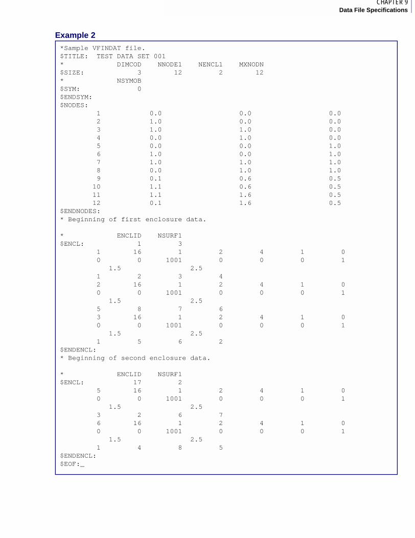
1CHAPTER 9Data File Specifications
Example 2*Sample VFINDAT file.$TITLE: TEST DATA SET 001* DIMCOD NNODE1 NENCL1 MXNODN$SIZE: 3 12 2 12* NSYMOB$SYM: 0$ENDSYM:$NODES: 1 0.0 0.0 0.0 2 1.0 0.0 0.0 3 1.0 1.0 0.0 4 0.0 1.0 0.0 5 0.0 0.0 1.0 6 1.0 0.0 1.0 7 1.0 1.0 1.0 8 0.0 1.0 1.0 9 0.1 0.6 0.5 10 1.1 0.6 0.5 11 1.1 1.6 0.5 12 0.1 1.6 0.5$ENDNODES:* Beginning of first enclosure data.
* ENCLID NSURF1$ENCL: 1 3 1 16 1 2 4 1 0 0 0 1001 0 0 0 1 1.5 2.5 1 2 3 4 2 16 1 2 4 1 0 0 0 1001 0 0 0 1 1.5 2.5 5 8 7 6 3 16 1 2 4 1 0 0 0 1001 0 0 0 1 1.5 2.5 1 5 6 2$ENDENCL:* Beginning of second enclosure data.
* ENCLID NSURF1$ENCL: 17 2 5 16 1 2 4 1 0 0 0 1001 0 0 0 1 1.5 2.5 3 2 6 7 6 16 1 2 4 1 0 0 0 1001 0 0 0 1 1.5 2.5 1 4 8 5$ENDENCL:$EOF:_
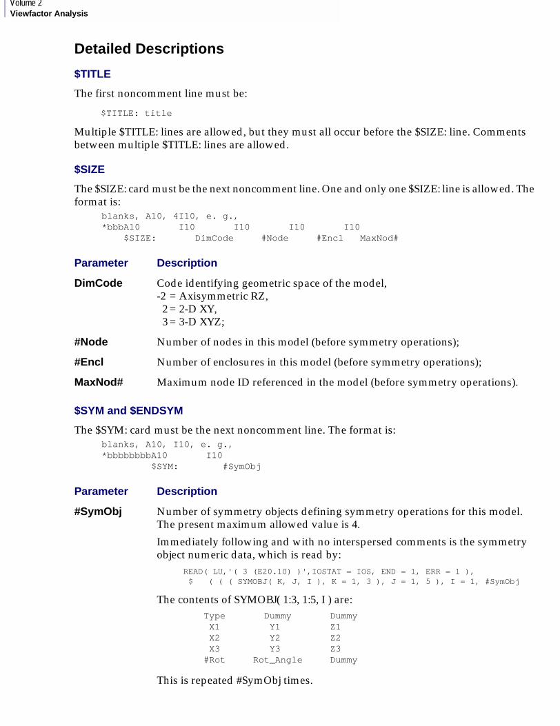
Volume 2Viewfactor Analysis
Detailed Descriptions
$TITLE
The first noncomment line must be:
$TITLE: title
Multiple $TITLE: lines are allowed, but they must all occur before the $SIZE: line. Comments between multiple $TITLE: lines are allowed.
$SIZE
The $SIZE: card must be the next noncomment line. One and only one $SIZE: line is allowed. The format is:
$SYM and $ENDSYM
The $SYM: card must be the next noncomment line. The format is:
Parameter Description
DimCode Code identifying geometric space of the model,-2 = Axisymmetric RZ, 2 = 2-D XY, 3 = 3-D XYZ;
#Node Number of nodes in this model (before symmetry operations);
#Encl Number of enclosures in this model (before symmetry operations);
MaxNod# Maximum node ID referenced in the model (before symmetry operations).
Parameter Description
#SymObj Number of symmetry objects defining symmetry operations for this model. The present maximum allowed value is 4.
Immediately following and with no interspersed comments is the symmetry object numeric data, which is read by:
READ( LU,'( 3 (E20.10) )',IOSTAT = IOS, END = 1, ERR = 1 ), $ ( ( ( SYMOBJ( K, J, I ), K = 1, 3 ), J = 1, 5 ), I = 1, #SymObj
The contents of SYMOBJ( 1:3, 1:5, I ) are:
This is repeated #SymObj times.
blanks, A10, 4I10, e. g., *bbbA10 I10 I10 I10 I10 $SIZE: DimCode #Node #Encl MaxNod#
blanks, A10, I10, e. g., *bbbbbbbbA10 I10 $SYM: #SymObj
Type Dummy Dummy X1 Y1 Z1 X2 Y2 Z2 X3 Y3 Z3
#Rot Rot_Angle Dummy
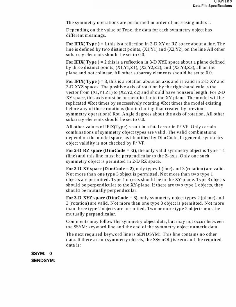
1CHAPTER 9Data File Specifications
The symmetry operations are performed in order of increasing index I.
Depending on the value of Type, the data for each symmetry object has different meanings.
For IFIX( Type ) = 1 this is a reflection in 2-D XY or RZ space about a line. The line is defined by two distinct points, (X1,Y1) and (X2,Y2), on the line All other subarray elements should be set to 0.0.
For IFIX( Type ) = 2 this is a reflection in 3-D XYZ space about a plane defined by three distinct points, (X1,Y1,Z1), (X2,Y2,Z2), and (X3,Y3,Z3), all on the plane and not colinear. All other subarray elements should be set to 0.0.
For IFIX( Type ) = 3, this is a rotation about an axis and is valid in 2-D XY and 3-D XYZ spaces. The positive axis of rotation by the right-hand rule is the vector from (X1,Y1,Z1) to (X2,Y2,Z2) and should have nonzero length. For 2-D XY space, this axis must be perpendicular to the XY-plane. The model will be replicated #Rot times by successively rotating #Rot times the model existing before any of these rotations (but including that created by previous symmetry operations) Rot_Angle degrees about the axis of rotation. All other subarray elements should be set to 0.0.
All other values of IFIX(Type) result in a fatal error in P/VF. Only certain combinations of symmetry object types are valid. The valid combinations depend on the model space, as identified by DimCode. In general, symmetry object validity is not checked by P/VF.
For 2-D RZ space (DimCode = -2), the only valid symmetry object is Type = 1 (line) and this line must be perpendicular to the Z-axis. Only one such symmetry object is permitted in 2-D RZ space.
For 2-D XY space (DimCode = 2), only types 1 (line) and 3 (rotation) are valid. Not more than one type 3 object is permitted. Not more than two type 1 objects are permitted. Type 1 objects should be in the XY-plane. Type 3 objects should be perpendicular to the XY-plane. If there are two type 1 objects, they should be mutually perpendicular.
For 3-D XYZ space (DimCode = 3), only symmetry object types 2 (plane) and 3 (rotation) are valid. Not more than one type 3 object is permitted. Not more than three type 2 objects are permitted. Two or more type 2 objects must be mutually perpendicular.
Comments may follow the symmetry object data, but may not occur between the $SYM: keyword line and the end of the symmetry object numeric data.
The next required keyword line is $ENDSYM:. This line contains no other data. If there are no symmetry objects, the $SymObj is zero and the required data is:
$SYM: 0
$ENDSYM:
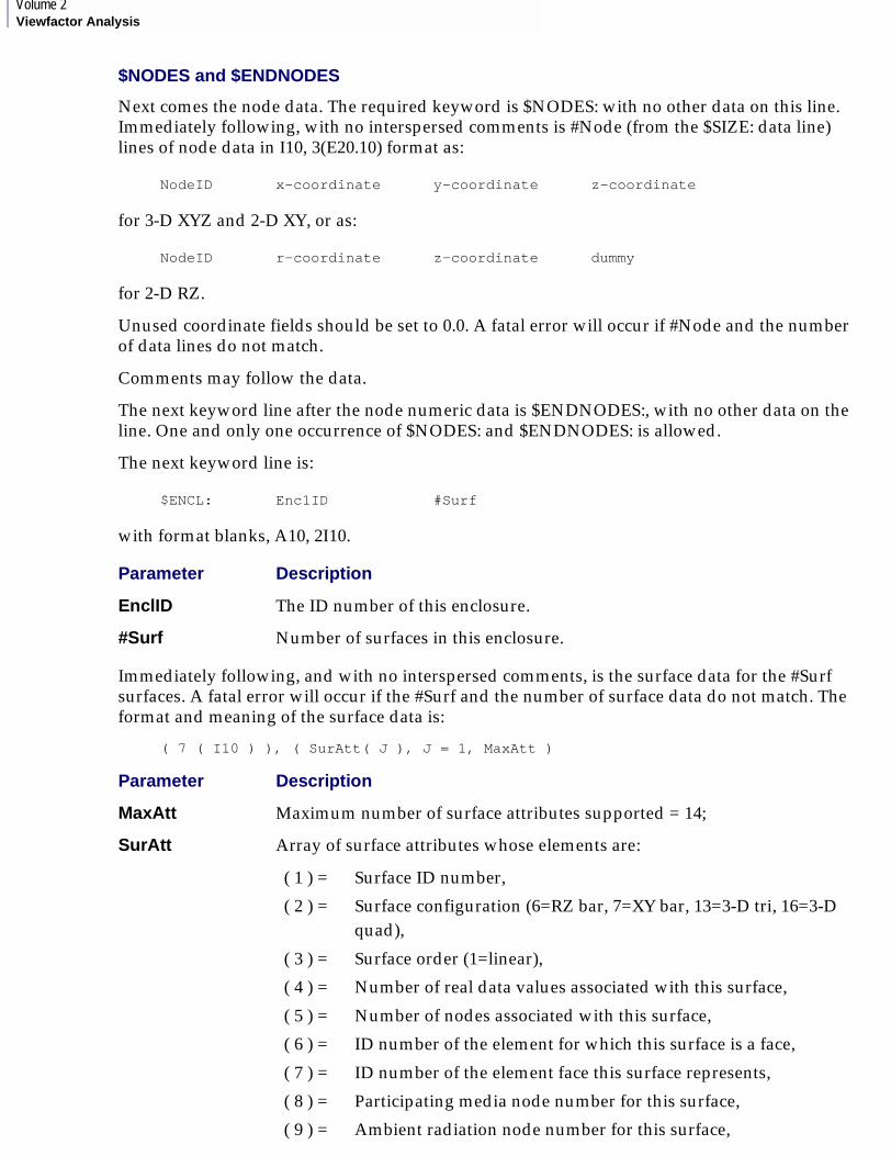
Volume 2Viewfactor Analysis
$NODES and $ENDNODES
Next comes the node data. The required keyword is $NODES: with no other data on this line. Immediately following, with no interspersed comments is #Node (from the $SIZE: data line) lines of node data in I10, 3(E20.10) format as:
for 3-D XYZ and 2-D XY, or as:
for 2-D RZ.
Unused coordinate fields should be set to 0.0. A fatal error will occur if #Node and the number of data lines do not match.
Comments may follow the data.
The next keyword line after the node numeric data is $ENDNODES:, with no other data on the line. One and only one occurrence of $NODES: and $ENDNODES: is allowed.
The next keyword line is:
with format blanks, A10, 2I10.
Immediately following, and with no interspersed comments, is the surface data for the #Surf surfaces. A fatal error will occur if the #Surf and the number of surface data do not match. The format and meaning of the surface data is:
( 7 ( I10 ) ), ( SurAtt( J ), J = 1, MaxAtt )
NodeID x-coordinate y-coordinate z-coordinate
NodeID r-coordinate z-coordinate dummy
$ENCL: Enc1ID #Surf
Parameter Description
EnclID The ID number of this enclosure.
#Surf Number of surfaces in this enclosure.
Parameter Description
MaxAtt Maximum number of surface attributes supported = 14;
SurAtt Array of surface attributes whose elements are:
( 1 ) = Surface ID number,
( 2 ) = Surface configuration (6=RZ bar, 7=XY bar, 13=3-D tri, 16=3-D quad),
( 3 ) = Surface order (1=linear),
( 4 ) = Number of real data values associated with this surface,
( 5 ) = Number of nodes associated with this surface,
( 6 ) = ID number of the element for which this surface is a face,
( 7 ) = ID number of the element face this surface represents,
( 8 ) = Participating media node number for this surface,
( 9 ) = Ambient radiation node number for this surface,
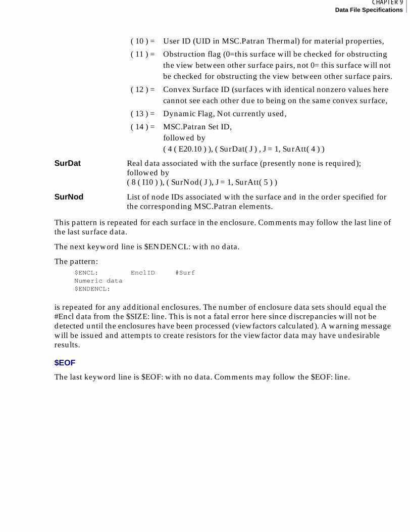
1CHAPTER 9Data File Specifications
This pattern is repeated for each surface in the enclosure. Comments may follow the last line of the last surface data.
The next keyword line is $ENDENCL: with no data.
The pattern:
is repeated for any additional enclosures. The number of enclosure data sets should equal the #Encl data from the $SIZE: line. This is not a fatal error here since discrepancies will not be detected until the enclosures have been processed (viewfactors calculated). A warning message will be issued and attempts to create resistors for the viewfactor data may have undesirable results.
$EOF
The last keyword line is $EOF: with no data. Comments may follow the $EOF: line.
( 10 ) = User ID (UID in MSC.Patran Thermal) for material properties,
( 11 ) = Obstruction flag (0=this surface will be checked for obstructing the view between other surface pairs, not 0= this surface will not be checked for obstructing the view between other surface pairs.
( 12 ) = Convex Surface ID (surfaces with identical nonzero values here cannot see each other due to being on the same convex surface,
( 13 ) = Dynamic Flag, Not currently used,
( 14 ) = MSC.Patran Set ID, followed by ( 4 ( E20.10 ) ), ( SurDat( J ) , J = 1, SurAtt( 4 ) )
SurDat Real data associated with the surface (presently none is required);followed by ( 8 ( I10 ) ), ( SurNod( J ), J = 1, SurAtt( 5 ) )
SurNod List of node IDs associated with the surface and in the order specified for the corresponding MSC.Patran elements.
$ENCL: EnclID #SurfNumeric data$ENDENCL:
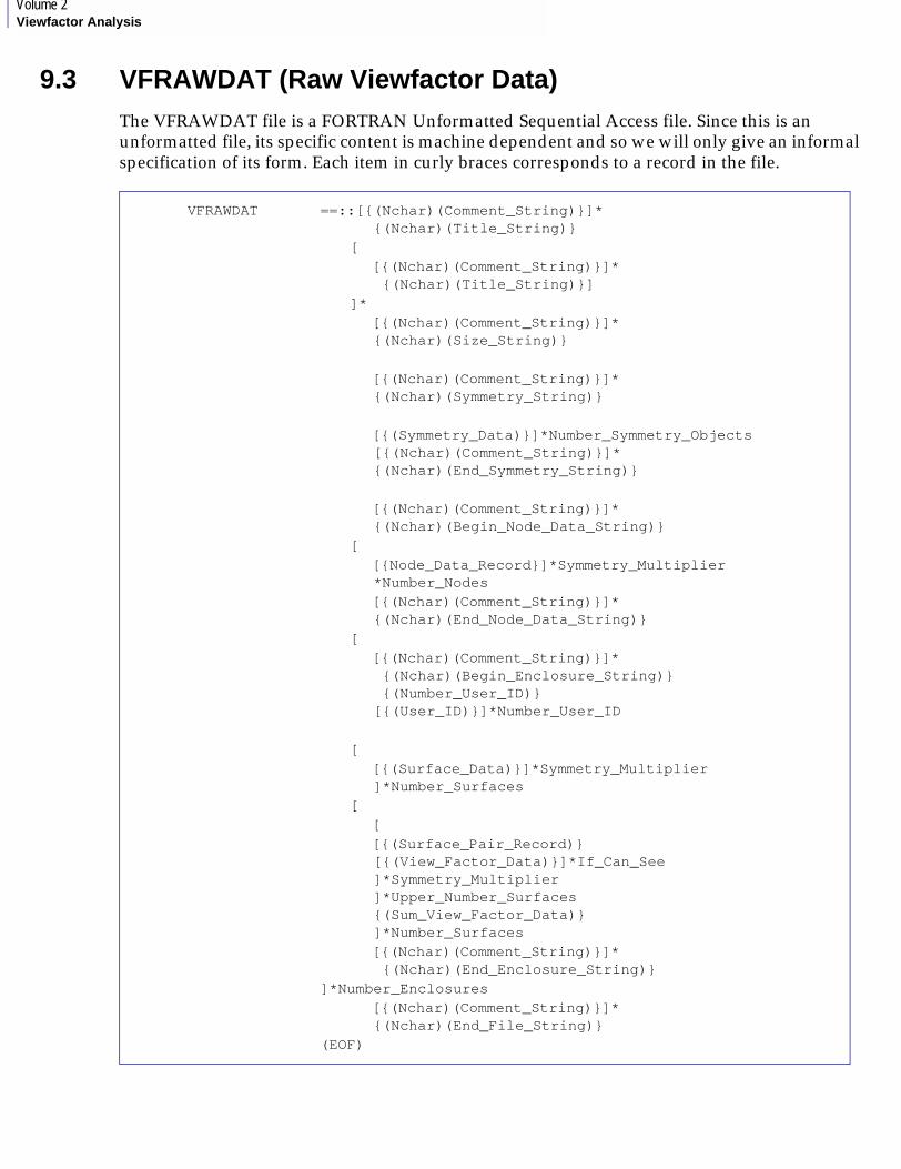
Volume 2Viewfactor Analysis
9.3 VFRAWDAT (Raw Viewfactor Data)The VFRAWDAT file is a FORTRAN Unformatted Sequential Access file. Since this is an unformatted file, its specific content is machine dependent and so we will only give an informal specification of its form. Each item in curly braces corresponds to a record in the file.
VFRAWDAT ==::[{(Nchar)(Comment_String)}]*{(Nchar)(Title_String)}
[[{(Nchar)(Comment_String)}]* {(Nchar)(Title_String)}]
]* [{(Nchar)(Comment_String)}]*
{(Nchar)(Size_String)}
[{(Nchar)(Comment_String)}]*{(Nchar)(Symmetry_String)}
[{(Symmetry_Data)}]*Number_Symmetry_Objects[{(Nchar)(Comment_String)}]*{(Nchar)(End_Symmetry_String)}
[{(Nchar)(Comment_String)}]*{(Nchar)(Begin_Node_Data_String)}
[[{Node_Data_Record}]*Symmetry_Multiplier*Number_Nodes[{(Nchar)(Comment_String)}]*{(Nchar)(End_Node_Data_String)}
[[{(Nchar)(Comment_String)}]* {(Nchar)(Begin_Enclosure_String)} {(Number_User_ID)}[{(User_ID)}]*Number_User_ID
[[{(Surface_Data)}]*Symmetry_Multiplier]*Number_Surfaces
[[[{(Surface_Pair_Record)}[{(View_Factor_Data)}]*If_Can_See]*Symmetry_Multiplier]*Upper_Number_Surfaces{(Sum_View_Factor_Data)}]*Number_Surfaces[{(Nchar)(Comment_String)}]* {(Nchar)(End_Enclosure_String)}
]*Number_Enclosures [{(Nchar)(Comment_String)}]*
{(Nchar)(End_File_String)} (EOF)
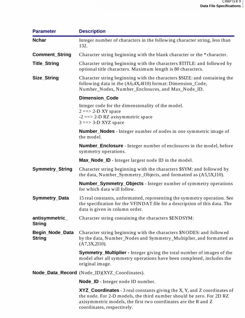
1CHAPTER 9Data File Specifications
Parameter Description
Nchar Integer number of characters in the following character string, less than 132.
Comment_String Character string beginning with the blank character or the * character.
Title_String Character string beginning with the characters $TITLE: and followed by optional title characters. Maximum length is 80 characters.
Size_String Character string beginning with the characters $SIZE: and containing the following data in the (A6,4X,4I10) format: Dimension_Code, Number_Nodes, Number_Enclosures, and Max_Node_ID.
Dimension_Code
Integer code for the dimensionality of the model.2 ==> 2-D XY space-2 ==> 2-D RZ axisymmetric space3 ==> 3-D XYZ space
Number_Nodes - Integer number of nodes in one symmetric image of the model.
Number_Enclosure - Integer number of enclosures in the model, before symmetry operations.
Max_Node_ID - Integer largest node ID in the model.
Symmetry_String Character string beginning with the characters $SYM: and followed by the data, Number_Symmetry_Objects, and formatted as (A5,5X,I10).
Number_Symmetry_Objects - Integer number of symmetry operations for which data will follow.
Symmetry_Data 15 real constants, unformatted, representing the symmetry operation. See the specification for the VFINDAT file for a description of this data. The data is given in column order.
antisymmetric_String
Character string containing the characters $ENDSYM:
Begin_Node_DataString
Character string beginning with the characters $NODES: and followed by the data, Number_Nodes and Symmetry_Multiplier, and formatted as (A7,3X,2I10).
Symmetry_Multiplier - Integer giving the total number of images of the model after all symmetry operations have been completed, includes the original image.
Node_Data_Record (Node_ID)(XYZ_Coordinates).
Node_ID - Integer node ID number.
XYZ_Coordinates - 3 real constants giving the X, Y, and Z coordinates of the node. For 2-D models, the third number should be zero. For 2D RZ axisymmetric models, the first two coordinates are the R and Z coordinates, respectively.
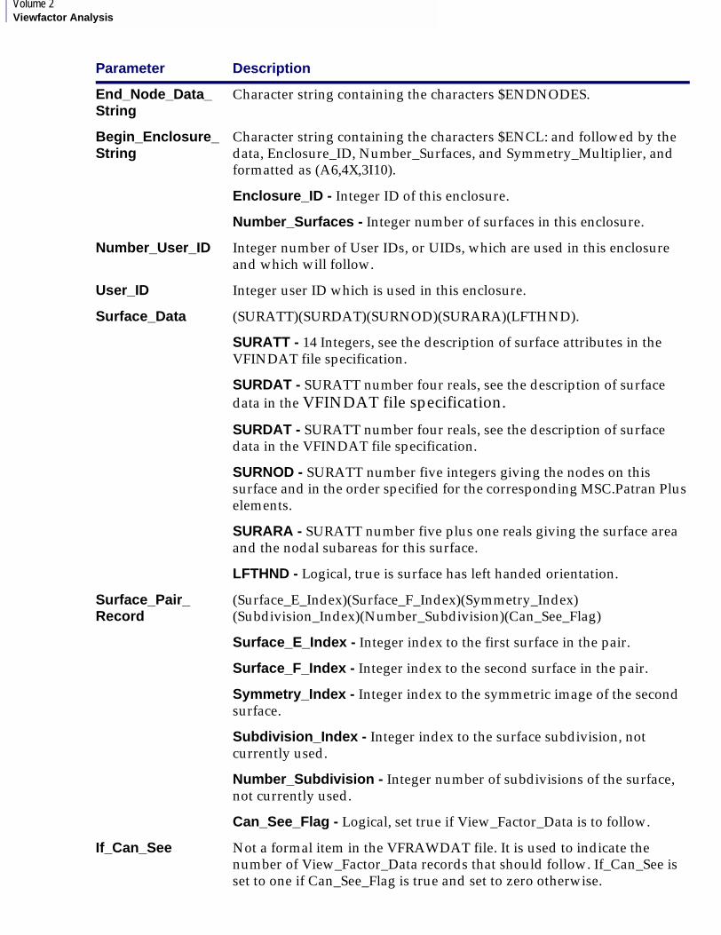
Volume 2Viewfactor Analysis
End_Node_Data_String
Character string containing the characters $ENDNODES.
Begin_Enclosure_String
Character string containing the characters $ENCL: and followed by the data, Enclosure_ID, Number_Surfaces, and Symmetry_Multiplier, and formatted as (A6,4X,3I10).
Enclosure_ID - Integer ID of this enclosure.
Number_Surfaces - Integer number of surfaces in this enclosure.
Number_User_ID Integer number of User IDs, or UIDs, which are used in this enclosure and which will follow.
User_ID Integer user ID which is used in this enclosure.
Surface_Data (SURATT)(SURDAT)(SURNOD)(SURARA)(LFTHND).
SURATT - 14 Integers, see the description of surface attributes in the VFINDAT file specification.
SURDAT - SURATT number four reals, see the description of surface data in the VFINDAT file specification.
SURDAT - SURATT number four reals, see the description of surface data in the VFINDAT file specification.
SURNOD - SURATT number five integers giving the nodes on this surface and in the order specified for the corresponding MSC.Patran Plus elements.
SURARA - SURATT number five plus one reals giving the surface area and the nodal subareas for this surface.
LFTHND - Logical, true is surface has left handed orientation.
Surface_Pair_Record
(Surface_E_Index)(Surface_F_Index)(Symmetry_Index) (Subdivision_Index)(Number_Subdivision)(Can_See_Flag)
Surface_E_Index - Integer index to the first surface in the pair.
Surface_F_Index - Integer index to the second surface in the pair.
Symmetry_Index - Integer index to the symmetric image of the second surface.
Subdivision_Index - Integer index to the surface subdivision, not currently used.
Number_Subdivision - Integer number of subdivisions of the surface, not currently used.
Can_See_Flag - Logical, set true if View_Factor_Data is to follow.
If_Can_See Not a formal item in the VFRAWDAT file. It is used to indicate the number of View_Factor_Data records that should follow. If_Can_See is set to one if Can_See_Flag is true and set to zero otherwise.
Parameter Description
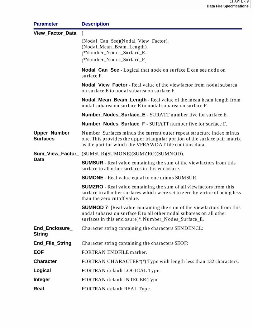
1CHAPTER 9Data File Specifications
View_Factor_Data [
(Nodal_Can_See)(Nodal_View_Factor).(Nodal_Mean_Beam_Length).]*Number_Nodes_Surface_E.
]*Number_Nodes_Surface_F.
Nodal_Can_See - Logical that node on surface E can see node on surface F.
Nodal_View_Factor - Real value of the viewfactor from nodal subarea on surface E to nodal subarea on surface F.
Nodal_Mean_Beam_Length - Real value of the mean beam length from nodal subarea on surface E to nodal subarea on surface F.
Number_Nodes_Surface_E - SURATT number five for surface E.
Number_Nodes_Surface_F - SURATT number five for surface F.
Upper_Number_Surfaces
Number_Surfaces minus the current outer repeat structure index minus one. This provides the upper triangular portion of the surface pair matrix as the part for which the VFRAWDAT file contains data.
Sum_View_Factor_Data
(SUMSUR)(SUMONE)(SUMZRO)(SUMNOD).
SUMSUR - Real value containing the sum of the viewfactors from this surface to all other surfaces in this enclosure.
SUMONE - Real value equal to one minus SUMSUR.
SUMZRO - Real value containing the sum of all viewfactors from this surface to all other surfaces which were set to zero by virtue of being less than the zero cutoff value.
SUMNOD 7- [Real value containing the sum of the viewfactors from this nodal subarea on surface E to all other nodal subareas on all other surfaces in this enclosure]*. Number_Nodes_Surface_E.
End_Enclosure_String
Character string containing the characters $ENDENCL:
End_File_String Character string containing the characters $EOF:
EOF FORTRAN ENDFILE marker.
Character FORTRAN CHARACTER*(*) Type with length less than 132 characters.
Logical FORTRAN default LOGICAL Type.
Integer FORTRAN default INTEGER Type.
Real FORTRAN default REAL Type.
Parameter Description
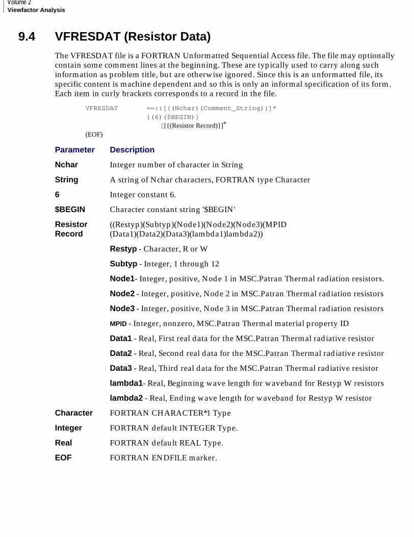
Volume 2Viewfactor Analysis
9.4 VFRESDAT (Resistor Data)The VFRESDAT file is a FORTRAN Unformatted Sequential Access file. The file may optionally contain some comment lines at the beginning. These are typically used to carry along such information as problem title, but are otherwise ignored. Since this is an unformatted file, its specific content is machine dependent and so this is only an informal specification of its form. Each item in curly brackets corresponds to a record in the file.
VFRESDAT ==::[{(Nchar)(Comment_String)}]*{(6)($BEGIN)}
[[{(Resistor Record)}]*
(EOF)
Parameter Description
Nchar Integer number of character in String
String A string of Nchar characters, FORTRAN type Character
6 Integer constant 6.
$BEGIN Character constant string '$BEGIN'
Resistor Record
((Restyp)(Subtyp)(Node1)(Node2)(Node3)(MPID(Data1)(Data2)(Data3)(lambda1)lambda2))
Restyp - Character, R or W
Subtyp - Integer, 1 through 12
Node1- Integer, positive, Node 1 in MSC.Patran Thermal radiation resistors.
Node2 - Integer, positive, Node 2 in MSC.Patran Thermal radiation resistors
Node3 - Integer, positive, Node 3 in MSC.Patran Thermal radiation resistors
MPID - Integer, nonzero, MSC.Patran Thermal material property ID
Data1 - Real, First real data for the MSC.Patran Thermal radiative resistor
Data2 - Real, Second real data for the MSC.Patran Thermal radiative resistor
Data3 - Real, Third real data for the MSC.Patran Thermal radiative resistor
lambda1- Real, Beginning wave length for waveband for Restyp W resistors
lambda2 - Real, Ending wave length for waveband for Restyp W resistor
Character FORTRAN CHARACTER*1 Type
Integer FORTRAN default INTEGER Type.
Real FORTRAN default REAL Type.
EOF FORTRAN ENDFILE marker.
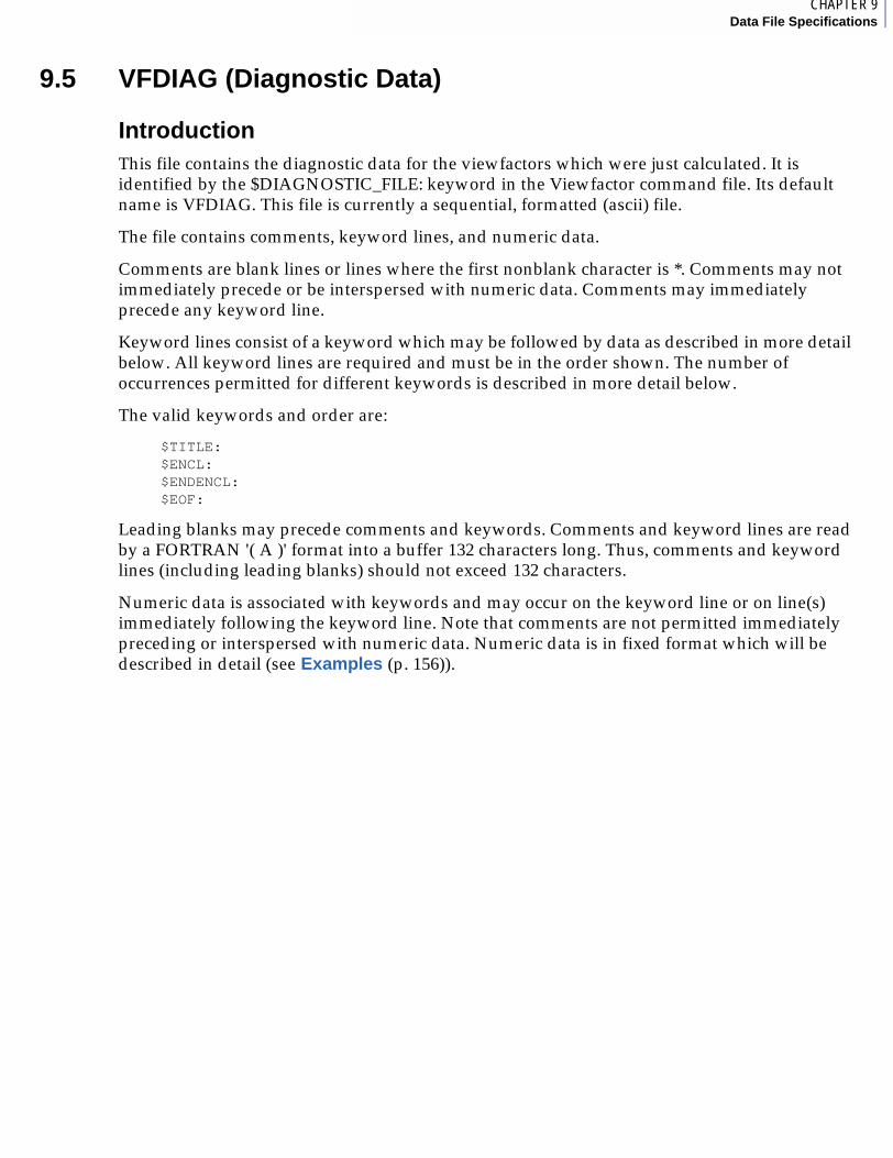
1CHAPTER 9Data File Specifications
9.5 VFDIAG (Diagnostic Data)
IntroductionThis file contains the diagnostic data for the viewfactors which were just calculated. It is identified by the $DIAGNOSTIC_FILE: keyword in the Viewfactor command file. Its default name is VFDIAG. This file is currently a sequential, formatted (ascii) file.
The file contains comments, keyword lines, and numeric data.
Comments are blank lines or lines where the first nonblank character is *. Comments may not immediately precede or be interspersed with numeric data. Comments may immediately precede any keyword line.
Keyword lines consist of a keyword which may be followed by data as described in more detail below. All keyword lines are required and must be in the order shown. The number of occurrences permitted for different keywords is described in more detail below.
The valid keywords and order are:
$TITLE:$ENCL:$ENDENCL:$EOF:
Leading blanks may precede comments and keywords. Comments and keyword lines are read by a FORTRAN '( A )' format into a buffer 132 characters long. Thus, comments and keyword lines (including leading blanks) should not exceed 132 characters.
Numeric data is associated with keywords and may occur on the keyword line or on line(s) immediately following the keyword line. Note that comments are not permitted immediately preceding or interspersed with numeric data. Numeric data is in fixed format which will be described in detail (see Examples (p. 156)).
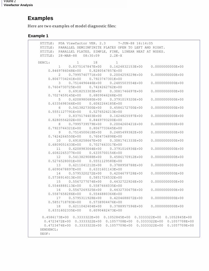
Volume 2Viewfactor Analysis
ExamplesHere are two examples of model diagnostic files:
Example 1
$TITLE: PDA Viewfactor VER. 2.3 7-JUN-88 16:14:05 $TITLE: PARALLEL SEMIINFINITE PLATES OPEN TO LEFT AND RIGHT. $TITLE: PARALLEL PLATES, SIMPLE, FINE, LINEAR HEAT AT NODES. $TITLE: 28-MAR-88 08:30:09 2.2K-X
$ENCL: 1 18 1 1 0.8375167847E+00 0.1624832153E+00 0.0000000000E+00 0.8469786048E+00 0.8280547857E+00 2 0.7995740771E+00 0.2004259229E+00 0.0000000000E+00 0.8067734241E+00 0.7923747301E+00 3 0.7514496446E+00 0.2485503554E+00 0.0000000000E+00 0.7604730725E+00 0.7424262762E+00 4 0.6918253303E+00 0.3081746697E+00 0.0000000000E+00 0.7027459145E+00 0.6809046268E+00 5 0.6208980680E+00 0.3791019320E+00 0.0000000000E+00 0.6335698366E+00 0.6082264185E+00 6 0.5413827300E+00 0.4586172700E+00 0.0000000000E+00 0.5551127791E+00 0.5276526213E+00 7 0.8375174403E+00 0.1624825597E+00 0.0000000000E+00 0.8280556202E+00 0.8469793200E+00 8 0.7995739579E+00 0.2004260421E+00 0.0000000000E+00 0.7923744321E+00 0.8067733645E+00 9 0.7514500618E+00 0.2485499382E+00 0.0000000000E+00 0.7424264550E+00 0.7604734898E+00 10 0.6918258667E+00 0.3081741333E+00 0.0000000000E+00 0.6809051633E+00 0.7027463317E+00 11 0.6208983064E+00 0.3791016936E+00 0.0000000000E+00 0.6082265377E+00 0.6335700154E+00 12 0.5413829088E+00 0.4586170912E+00 0.0000000000E+00 0.5276528001E+00 0.5551129580E+00 13 0.6211041212E+00 0.3788958788E+00 0.0000000000E+00 0.6090478897E+00 0.6331601143E+00 14 0.5795320272E+00 0.4204679728E+00 0.0000000000E+00 0.5738914013E+00 0.5851726532E+00 15 0.5567277074E+00 0.4432722926E+00 0.0000000000E+00 0.5546888113E+00 0.5587666035E+00 16 0.5567269325E+00 0.4432730675E+00 0.0000000000E+00 0.5587658286E+00 0.5546880364E+00 17 0.5795311928E+00 0.4204688072E+00 0.0000000000E+00 0.5851718783E+00 0.5738904476E+00 18 0.6211042404E+00 0.3788957596E+00 0.0000000000E+00 0.6331602335E+00 0.6090482473E+00
0.4586173E+00 0.3333322E+00 0.1052845E+00 0.3333322E+00 0.1052845E+00 0.4723472E+00 0.3333322E+00 0.1057708E+00 0.3333322E+00 0.1057708E+00 0.4723474E+00 0.3333322E+00 0.1057709E+00 0.3333322E+00 0.1057709E+00 $ENDENCL: $EOF:
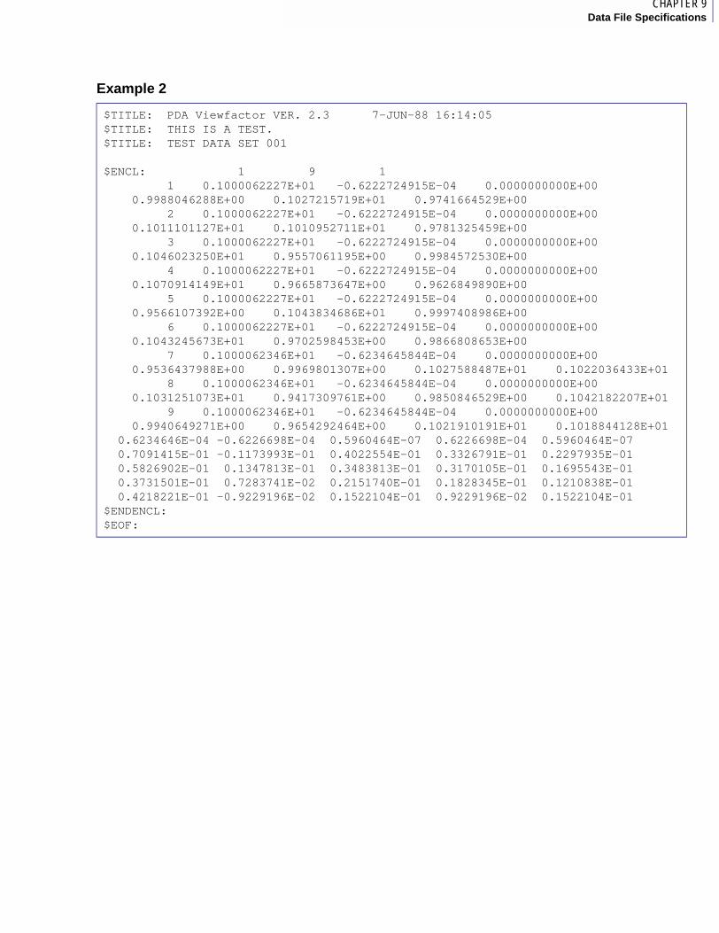
1CHAPTER 9Data File Specifications
Example 2
$TITLE: PDA Viewfactor VER. 2.3 7-JUN-88 16:14:05 $TITLE: THIS IS A TEST. $TITLE: TEST DATA SET 001 $ENCL: 1 9 1 1 0.1000062227E+01 -0.6222724915E-04 0.0000000000E+00 0.9988046288E+00 0.1027215719E+01 0.9741664529E+00 2 0.1000062227E+01 -0.6222724915E-04 0.0000000000E+00 0.1011101127E+01 0.1010952711E+01 0.9781325459E+00 3 0.1000062227E+01 -0.6222724915E-04 0.0000000000E+00 0.1046023250E+01 0.9557061195E+00 0.9984572530E+00 4 0.1000062227E+01 -0.6222724915E-04 0.0000000000E+00 0.1070914149E+01 0.9665873647E+00 0.9626849890E+00 5 0.1000062227E+01 -0.6222724915E-04 0.0000000000E+00 0.9566107392E+00 0.1043834686E+01 0.9997408986E+00 6 0.1000062227E+01 -0.6222724915E-04 0.0000000000E+00 0.1043245673E+01 0.9702598453E+00 0.9866808653E+00 7 0.1000062346E+01 -0.6234645844E-04 0.0000000000E+00 0.9536437988E+00 0.9969801307E+00 0.1027588487E+01 0.1022036433E+01 8 0.1000062346E+01 -0.6234645844E-04 0.0000000000E+00 0.1031251073E+01 0.9417309761E+00 0.9850846529E+00 0.1042182207E+01 9 0.1000062346E+01 -0.6234645844E-04 0.0000000000E+00 0.9940649271E+00 0.9654292464E+00 0.1021910191E+01 0.1018844128E+01 0.6234646E-04 -0.6226698E-04 0.5960464E-07 0.6226698E-04 0.5960464E-07 0.7091415E-01 -0.1173993E-01 0.4022554E-01 0.3326791E-01 0.2297935E-01 0.5826902E-01 0.1347813E-01 0.3483813E-01 0.3170105E-01 0.1695543E-01 0.3731501E-01 0.7283741E-02 0.2151740E-01 0.1828345E-01 0.1210838E-01 0.4218221E-01 -0.9229196E-02 0.1522104E-01 0.9229196E-02 0.1522104E-01 $ENDENCL: $EOF:

Volume 2Viewfactor Analysis
Detailed Descriptions
$TITLE
The first noncomment line must be:
$TITLE: title
Multiple $TITLE: lines are allowed, but they must all occur before the $ENCL: line. Comments between multiple $TITLE: lines are allowed.
$ENCL and $ENDENCL
The next keyword line is:
with format blanks, A10, 3I10.
Immediately following, and with no interspersed comments, is the surface data for the #Surf surfaces. A fatal error will occur if the #Surf and the number of surface data do not match. The format and meaning of the surface data is:
( 1X, I10, 3E19.10 ) SURID, SUMSUR, SUMONE, SUMZRO( 1X, 4E19.10 ) ( SUMNOD( I ), J = 1, NNODE ).
This pattern is repeated for each surface in the enclosure. After this data has been given for all surfaces in the enclosure, some additional statistical data for the enclosure is given. The format and meaning of the statistical data is:
( 1X, 5E15.7 ) ( MX( J ), AV( J ), SD( J ), AB( J ), ASD( J ) ), J = 0, MXND )
Parameter Description
EnclID The ID number of this enclosure
#Surf Number of surfaces in this enclosure,
SymMul Number of symmetric images of each surface.
Parameter Description
SURID Surface ID;
SUMSUR Sum of the viewfactors from this surface to all other surfaces in this enclosure;
SUMONE 1.0 - SUMSUR;
SUMZRO Sum of the viewfactors from this surface to all other surfaces in this enclosure which were set to zero by virtue of being less than the zero cutoff value;
SUMNOD Sum of the viewfactors from each nodal subarea on this surface to all other nodal subarea on all other surfaces in this enclosure;
J Index to the nodal subareas on this surface;
NNODE Number of nodes on this surface.
$ENCL: EnclID #Surf SymMul

1CHAPTER 9Data File Specifications
The next keyword line is $ENDENCL: with no data.
The pattern:
is repeated for any additional enclosures.
$EOF
The last keyword line is $EOF: with no data. Comments may follow the $EOF: line.
Parameter Description
MX Maximum absolute deviation from unity for the sums of viewfactors;
AV Average deviation from unity for the sums of viewfactors;
SD Standard deviation of the data used to calculate AV;
AB Average absolute deviation from unity for the sums of viewfactors;
ASD Standard deviation of the data used to calculate AB;
J Index, 0 = entire surface, 1 through MXND = nodal subareas;
MXND Maximum number of nodes on any surface in this enclosure.
$ENCL: EnclID #Surf SymMulNumeric data$ENDENCL:
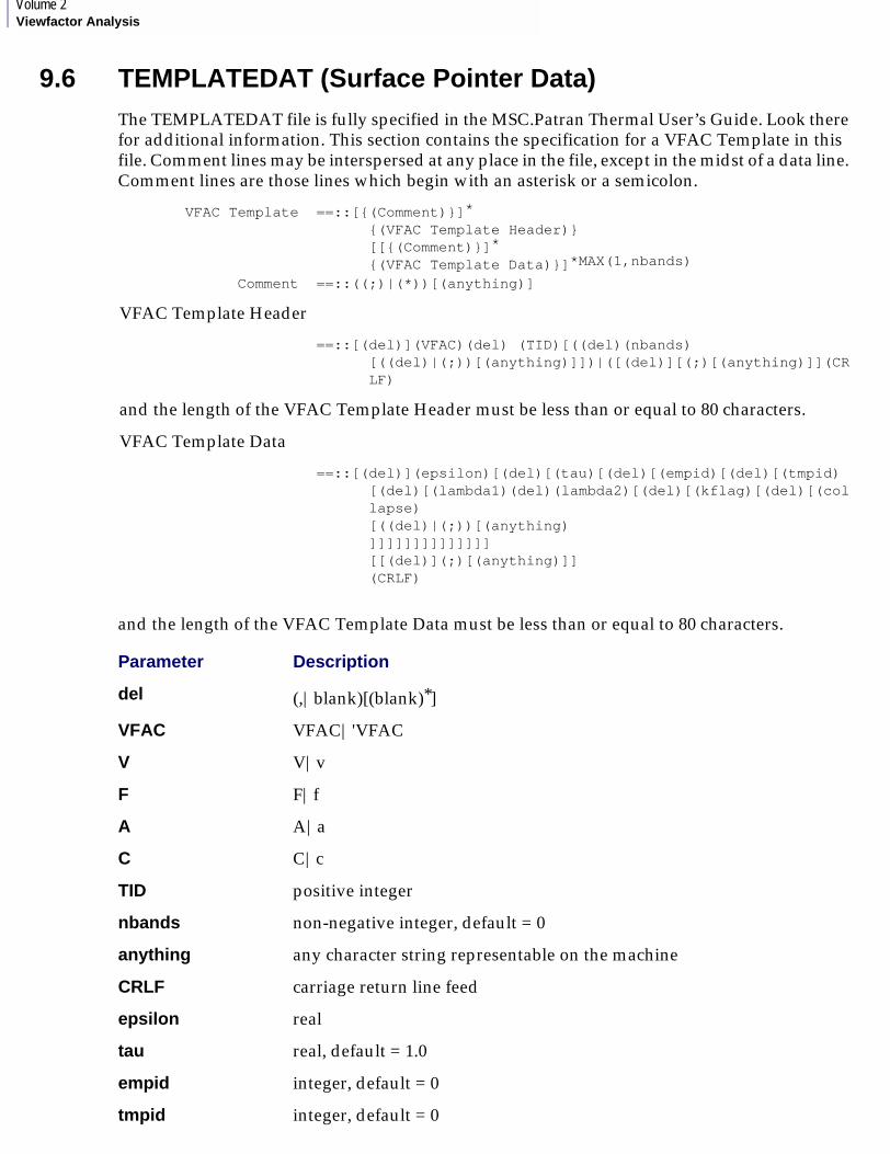
Volume 2Viewfactor Analysis
9.6 TEMPLATEDAT (Surface Pointer Data)The TEMPLATEDAT file is fully specified in the MSC.Patran Thermal User’s Guide. Look there for additional information. This section contains the specification for a VFAC Template in this file. Comment lines may be interspersed at any place in the file, except in the midst of a data line. Comment lines are those lines which begin with an asterisk or a semicolon.
and the length of the VFAC Template Data must be less than or equal to 80 characters.
Parameter Description
del (,|blank)[(blank)*]
VFAC VFAC|'VFAC
V V|v
F F|f
A A|a
C C|c
TID positive integer
nbands non-negative integer, default = 0
anything any character string representable on the machine
CRLF carriage return line feed
epsilon real
tau real, default = 1.0
empid integer, default = 0
tmpid integer, default = 0
VFAC Template ==::[{(Comment)}]*
{(VFAC Template Header)}[[{(Comment)}]*
{(VFAC Template Data)}]*MAX(1,nbands)
Comment ==::((;)|(*))[(anything)]
VFAC Template Header
==::[(del)](VFAC)(del) (TID)[((del)(nbands)[((del)|(;))[(anything)]])|([(del)][(;)[(anything)]](CRLF)
and the length of the VFAC Template Header must be less than or equal to 80 characters.
VFAC Template Data
==::[(del)](epsilon)[(del)[(tau)[(del)[(empid)[(del)[(tmpid) [(del)[(lambda1)(del)(lambda2)[(del)[(kflag)[(del)[(collapse)[((del)|(;))[(anything)]]]]]]]]]]]]]][[(del)](;)[(anything)]](CRLF)

1CHAPTER 9Data File Specifications
In addition to the above form requirements, only certain combinations of data values are valid. These are determined by the following tests:
1. If nbands equals 0 and either lambda1 not equal to 0.0 or lambda2 not equal to 0.0, then this is an error.
2. If nbands greater than 0 and either lambda1 greater than or equal to lambda2 or lambda 1 less than 0.0, then this is an error.
3. If kflag is not equal to 0 or 1, then this is an error.
4. If empid equals 0 and either epsilon is less than or equal to 0.0 or epsilon is greater than 1.0, then this is an error.
5. If empid is not equal to 0 and epsilon is not equal to 0.0, then this is an error.
6. If tmpid equals 0 and kflag equals 0 and either tau is less than or equal to 0.0 or tau is greater than 1.0, then this is an error.
7. If tmpid equals 0 and kflag equals 1 and tau is less than 0.0, then this is an error.
8. If tmpid is not equal to 0 and tau is not equal to 0.0, then this is an error.
Additionally, an error will occur in Viewfactor if tmpid is not equal to 0, and there is not a MEDNOD available with the referenced surface or if kflag equals 1, and an AMBNOD is associated with the reverenced surface.
lambda1 real, default = 0.0
lambda2 real, default = 0.0
kflag integer, default = 0
collapse non-negative integer, default = 0
real Real number representable on the machine in default real type variable and having 20 or less digits, including +, -, ., E, etc. Default format is G20.10
integer Integer number representable on the machine in default integer type variable and having 20 or less digits, including +, -, etc.
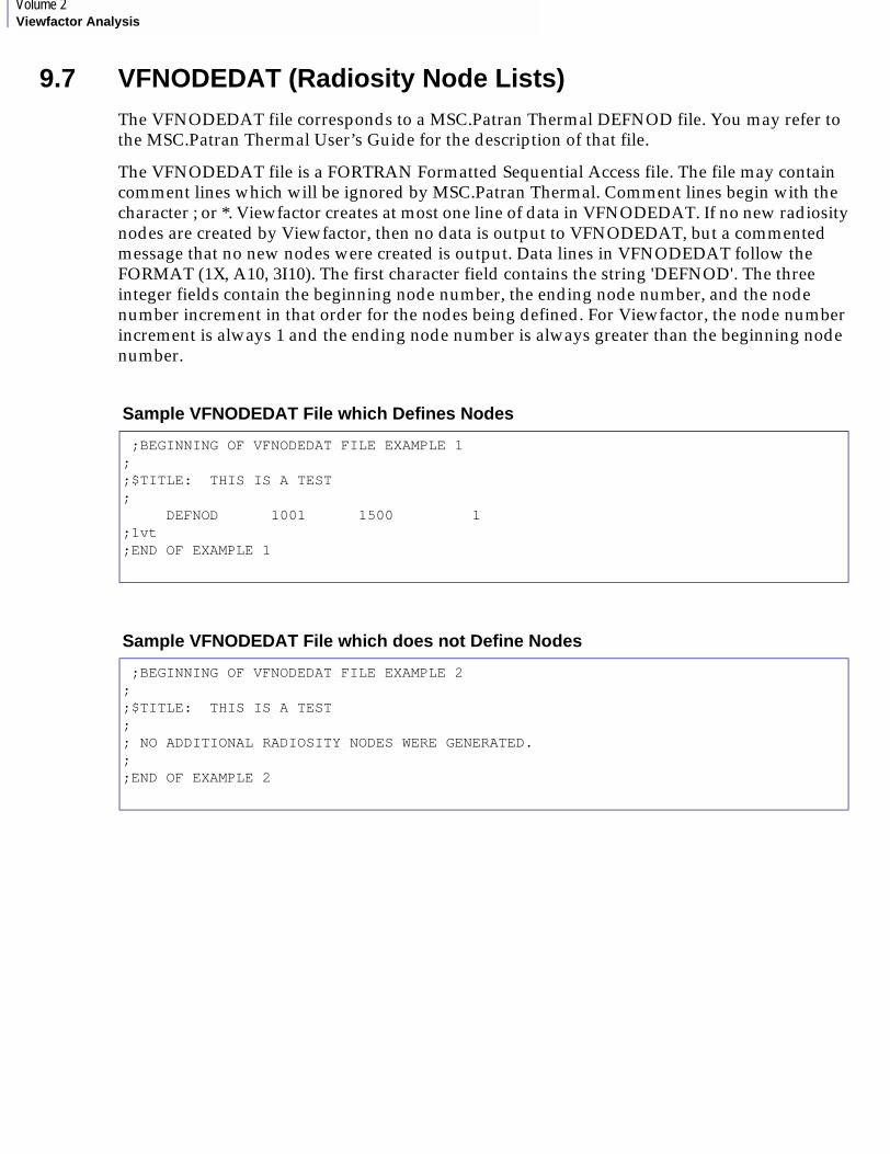
Volume 2Viewfactor Analysis
9.7 VFNODEDAT (Radiosity Node Lists)The VFNODEDAT file corresponds to a MSC.Patran Thermal DEFNOD file. You may refer to the MSC.Patran Thermal User’s Guide for the description of that file.
The VFNODEDAT file is a FORTRAN Formatted Sequential Access file. The file may contain comment lines which will be ignored by MSC.Patran Thermal. Comment lines begin with the character ; or *. Viewfactor creates at most one line of data in VFNODEDAT. If no new radiosity nodes are created by Viewfactor, then no data is output to VFNODEDAT, but a commented message that no new nodes were created is output. Data lines in VFNODEDAT follow the FORMAT (1X, A10, 3I10). The first character field contains the string 'DEFNOD'. The three integer fields contain the beginning node number, the ending node number, and the node number increment in that order for the nodes being defined. For Viewfactor, the node number increment is always 1 and the ending node number is always greater than the beginning node number.
Sample VFNODEDAT File which Defines Nodes
;BEGINNING OF VFNODEDAT FILE EXAMPLE 1;;$TITLE: THIS IS A TEST; DEFNOD 1001 1500 1;1vt;END OF EXAMPLE 1
Sample VFNODEDAT File which does not Define Nodes
;BEGINNING OF VFNODEDAT FILE EXAMPLE 2;;$TITLE: THIS IS A TEST;; NO ADDITIONAL RADIOSITY NODES WERE GENERATED.;;END OF EXAMPLE 2

MSC.Patran Thermal User’s Guide, Volume 2: Viewfactor Analysis
CHAPTER
10 Rules for Radiation Resistors
■ Introduction
■ General Rules for Radiation Resistors
■ Rules for Emissivity Resistors
■ Rules for Radiosity Resistors

1CHAPTER 10Rules for Radiation Resistors
10.1 IntroductionViewfactor uses rules to determine which MSC.Patran Thermal radiation resistors to make. Which resistors are made depends on the data in the VFAC Templates and VFRAWDAT file. This chapter describes these rules. Restrictions on the valid ranges of data in the VFAC Templates is described in the previous chapter in the section on the VFAC Template data specification, VFRAWDAT (Raw Viewfactor Data) (p. 150). These will not be repeated here.

1CHAPTER 10Rules for Radiation Resistors
10.2 General Rules for Radiation ResistorsIf the value of nbands is zero, either by default or by specification, then the resistor type will be the MSC.Patran Thermal type R.
If the value of nbands is greater than zero, then the resistor type will be the MSC.Patran Thermal type W.

1CHAPTER 10Rules for Radiation Resistors
10.3 Rules for Emissivity ResistorsFor the emissivity resistors:
• If empid is zero and epsilon is one, then no emissivity resistor is made and the surface node will serve as the radiosity node for any radiosity resistors to be made.
• If empid is zero and epsilon is greater than zero but less than one, then a radiosity node will be created and joined to the surface node with a MSC.Patran Thermal subtype 5 resistor.
• If empid is not zero and epsilon is zero, then a radiosity node will be created and joined to the surface node with a MSC.Patran Thermal subtype 1 resistor.
• If Viewfactor detects a zero valued resistor, then that resistor will not be made and the surface node will serve as the radiosity node.
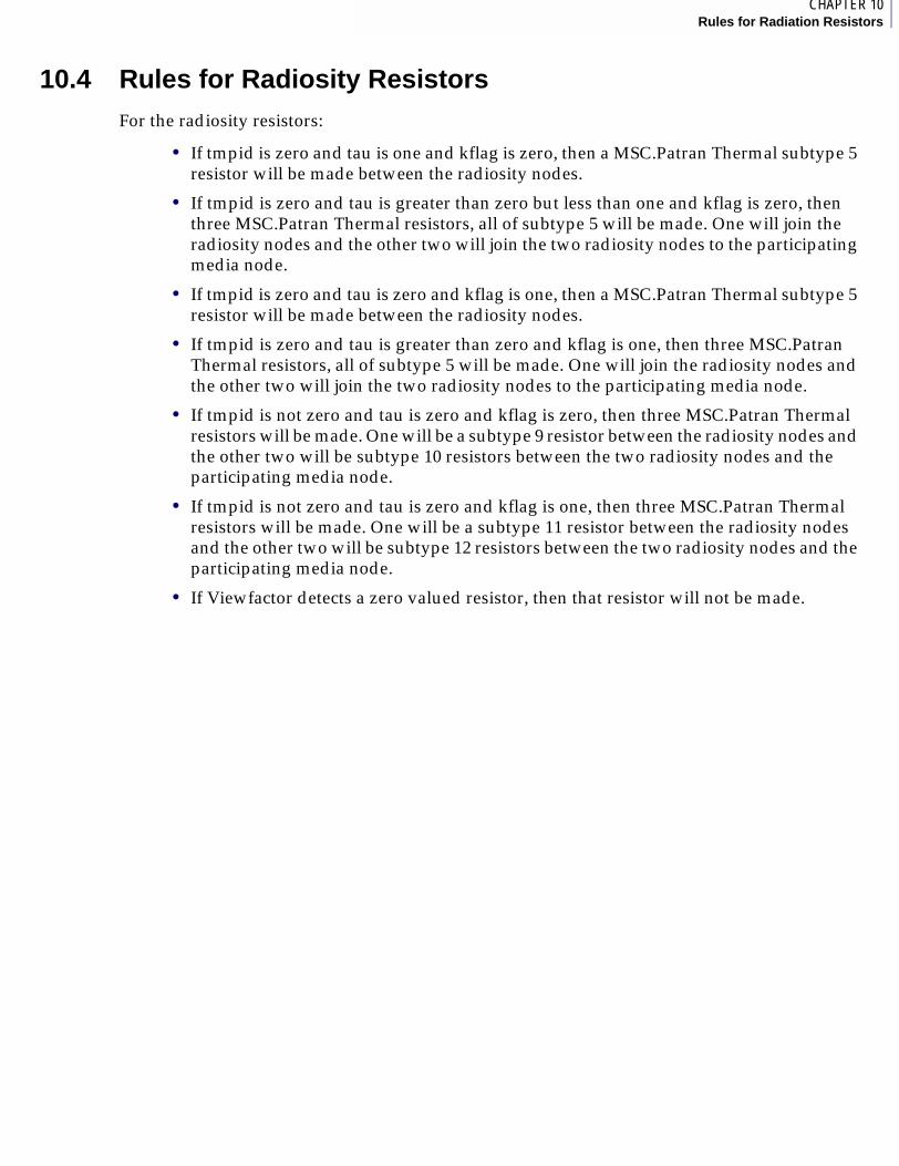
1CHAPTER 10Rules for Radiation Resistors
10.4 Rules for Radiosity Resistors For the radiosity resistors:
• If tmpid is zero and tau is one and kflag is zero, then a MSC.Patran Thermal subtype 5 resistor will be made between the radiosity nodes.
• If tmpid is zero and tau is greater than zero but less than one and kflag is zero, then three MSC.Patran Thermal resistors, all of subtype 5 will be made. One will join the radiosity nodes and the other two will join the two radiosity nodes to the participating media node.
• If tmpid is zero and tau is zero and kflag is one, then a MSC.Patran Thermal subtype 5 resistor will be made between the radiosity nodes.
• If tmpid is zero and tau is greater than zero and kflag is one, then three MSC.Patran Thermal resistors, all of subtype 5 will be made. One will join the radiosity nodes and the other two will join the two radiosity nodes to the participating media node.
• If tmpid is not zero and tau is zero and kflag is zero, then three MSC.Patran Thermal resistors will be made. One will be a subtype 9 resistor between the radiosity nodes and the other two will be subtype 10 resistors between the two radiosity nodes and the participating media node.
• If tmpid is not zero and tau is zero and kflag is one, then three MSC.Patran Thermal resistors will be made. One will be a subtype 11 resistor between the radiosity nodes and the other two will be subtype 12 resistors between the two radiosity nodes and the participating media node.
• If Viewfactor detects a zero valued resistor, then that resistor will not be made.

1CHAPTER 10Rules for Radiation Resistors

MSC.Patran Thermal User’s Guide, Volume 2: Viewfactor Analysis
APPENDIX
A Typical Errors and Probable Causes for Viewfactor Errors
■ Purpose

Volume 2Viewfactor Analysis
A.1 PurposeViewfactor performs extensive error checking and reporting. It utilizes an error message generator which creates error messages as needed from phrases stored in memory. In general, these error messages provide more information than we could supply with a reasonable number of error codes. Error messages, if any, will be found in the VFMSG file, along with a traceback of the subroutine calling sequence leading to the error condition. This traceback is provided because Viewfactor was designed to terminate normally, even under error conditions. It is the only way for us to know the program status associated with ^an error.
Some typical errors and their probable causes are:
File Errors These occur when an expected file is not present or available to the program, or a file to be created is already present. The solution is to make the expected file available or to remove or rename the file already present. The files referenced may also be changed by altering the names given in the VFCTL file.
Format Errors This means the data in a file is not in an acceptable format. This usually occurs with the TEMPLATEDAT file since this is usually the only data file which the user must build using the system editor.
UID/TID Errors Reference UIDs are not available in the VFAC TIDs. This error is corrected by adding the appropriate VFAC TID records to the TEMPLATEDAT file.
SurfaceIncompatibilityErrors
The properties assigned by the VFAC DFEG data and VFAC Template data to a pair of surfaces which can see each other in an enclosure are not compatible. For example, the surfaces might have a different number of wavebands assigned to each. For additional information, you can refer to Compatibility Requirements for Model and VFAC Templates (p. 75) and Introduction (p. 130) which address surface compatibility.
Note: Please refer back to Submitting a Viewfactor Job for Analysis (p. 108) and recheck each item called out for review prior to submitting a Viewfactor job.

MSC.Patran Thermal User’s Guide, Volume 2: Viewfactor Analysis
APPENDIX
B Quick Reference Guide to Viewfactor
■ Purpose

Volume 2Viewfactor Analysis
B.1 PurposeThe general procedure for performing a thermal radiation analysis is:
The MSC.Patran Plus VFAC boundary condition is:
The surfaces on which the VFAC boundary conditions are applied are defined under Application Region.
The VFAC Template in the MSC.Patran Thermal TEMPLATEDAT file has the form:
VFAC, TID, nbandsepsilon, tau, empid, tmpid, lambda1, lambda2, kflag, collapse
MSC.Patran Build model and assign boundary conditions.
Analysis Menu Select Viewfactor Solution under Solution Type.
Hit Apply This executes a script that will check for obstructions, calculate viewfactors and make radiation resistors for MSC.Patran Thermal.
Analysis Menu If a thermal analysis was requested under solution type, following the Viewfactor analysis, MSC.Patran Thermal will create a QTRAN source file for the problem and perform the thermal network analysis.
MSC.Patran Display the results.
Parameter Description
UID User template ID.
MEDNOD Participating media node if any Flag for top or bottom of shell.
AMBNOD Ambient or space node.
CNVSID Convex surface ID.
NONOBSTRUCTING FLAG
Flag for nonobstructing surface.
TOP/BOTTOM FLAG Flag for top or bottom of shell.
ENCLOSURE ID Enclosure ID.
Parameter Description
TID Integer, Template ID.
nbands Integer, Optional, Default = 0, Number of wavebands in this template.
epsilon Real, surface emissivity.
tau Real, Optional, Default = 1.0, Participating media transmissivity (kflag = 0) or extinction coefficient (kflag = 1).
empid Integer, Optional, Default = 0, Emissivity material property ID.
tmpid Integer, Optional, Default = 0, Transmissivity (kflag = 0) or extinction coefficient (kflag = 1) material property ID.

1APPENDIX BQuick Reference Guide to Viewfactor
The line,
epsilon, tau, empid, tmpid, lambda1, lambda2, kflag, collapse
must be repeated for each of the nbands in the template and once for nbands = 0.
The Viewfactor command line is:
VSUBMIT VFCTL
lambda1 Real, Optional, Default = 0.0, Waveband beginning wavelength, microns.
lambda2 Real, Optional, Default = 0.0, Waveband ending wavelength, microns.
kflag Integer, Optional, Default = 0, Flag that tau or tmpid refer to transmissivity (kflag = 1) or to extinction coefficient (kflag = 1).
collapse Integer, Optional, Default = 0, ID to control the collapsing of radiosity nodes associated with a surface node.
Parameter Description
Note: This command is automatically issued when execution is spawned from within MSC.Patran.
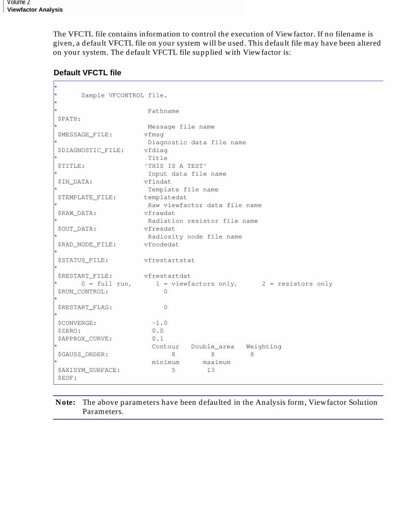
Volume 2Viewfactor Analysis
The VFCTL file contains information to control the execution of Viewfactor. If no filename is given, a default VFCTL file on your system will be used. This default file may have been altered on your system. The default VFCTL file supplied with Viewfactor is:
Note: The above parameters have been defaulted in the Analysis form, Viewfactor Solution Parameters.
Default VFCTL file
** Sample VFCONTROL file.** Pathname $PATH: * Message file name $MESSAGE_FILE: vfmsg* Diagnostic data file name $DIAGNOSTIC_FILE: vfdiag* Title $TITLE: 'THIS IS A TEST'* Input data file name $IN_DATA: vfindat* Template file name $TEMPLATE_FILE: templatedat* Raw viewfactor data file name $RAW_DATA: vfrawdat* Radiation resistor file name $OUT_DATA: vfresdat* Radiosity node file name $RAD_NODE_FILE: vfnodedat* $STATUS_FILE: vfrestartstat* $RESTART_FILE: vfrestartdat* 0 = full run, 1 = viewfactors only, 2 = resistors only $RUN_CONTROL: 0* $RESTART_FLAG: 0* $CONVERGE: -1.0 $ZERO: 0.0 $APPROX_CURVE: 0.1* Contour Double_area Weighting $GAUSS_ORDER: 8 8 8* minimum maximum $AXISYM_SURFACE: 5 13 $EOF:

MSC.Patran Thermal User’s Guide, Volume 2: Viewfactor Analysis
APPENDIX
C Memory Requirements for Viewfactor Execution
■ Purpose
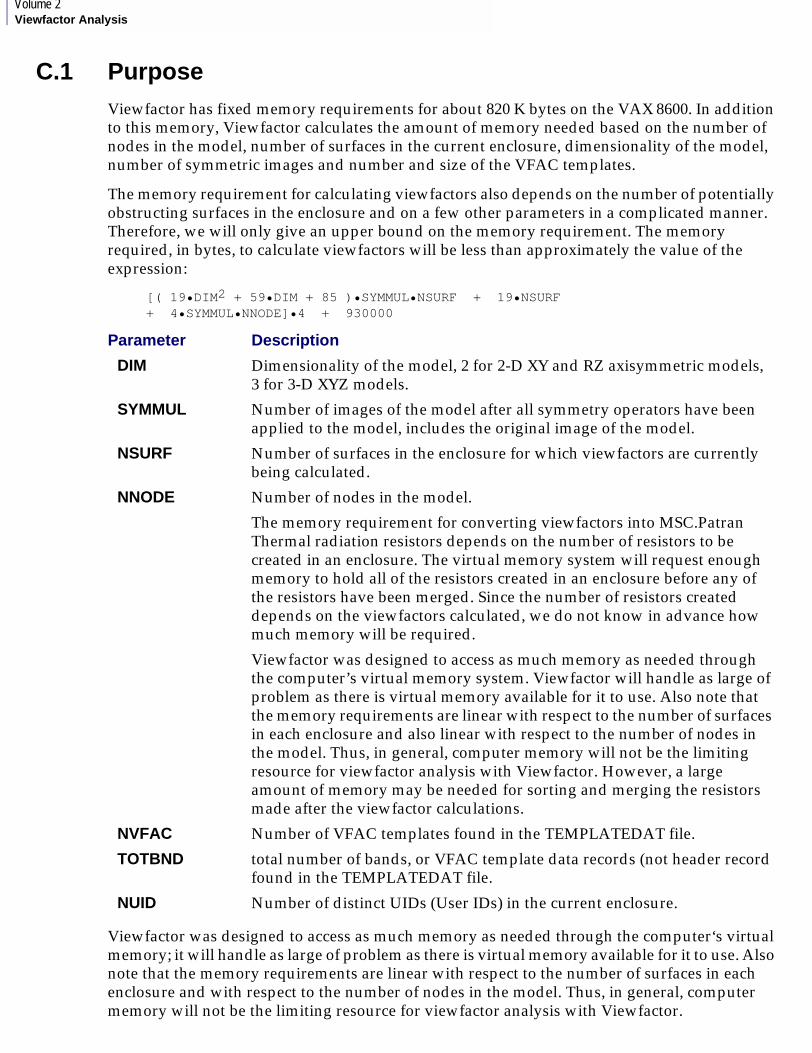
Volume 2Viewfactor Analysis
C.1 PurposeViewfactor has fixed memory requirements for about 820 K bytes on the VAX 8600. In addition to this memory, Viewfactor calculates the amount of memory needed based on the number of nodes in the model, number of surfaces in the current enclosure, dimensionality of the model, number of symmetric images and number and size of the VFAC templates.
The memory requirement for calculating viewfactors also depends on the number of potentially obstructing surfaces in the enclosure and on a few other parameters in a complicated manner. Therefore, we will only give an upper bound on the memory requirement. The memory required, in bytes, to calculate viewfactors will be less than approximately the value of the expression:
[( 19•DIM2 + 59•DIM + 85 )•SYMMUL•NSURF + 19•NSURF + 4•SYMMUL•NNODE]•4 + 930000
Viewfactor was designed to access as much memory as needed through the computer‘s virtual memory; it will handle as large of problem as there is virtual memory available for it to use. Also note that the memory requirements are linear with respect to the number of surfaces in each enclosure and with respect to the number of nodes in the model. Thus, in general, computer memory will not be the limiting resource for viewfactor analysis with Viewfactor.
Parameter Description
DIM Dimensionality of the model, 2 for 2-D XY and RZ axisymmetric models, 3 for 3-D XYZ models.
SYMMUL Number of images of the model after all symmetry operators have been applied to the model, includes the original image of the model.
NSURF Number of surfaces in the enclosure for which viewfactors are currently being calculated.
NNODE Number of nodes in the model.
The memory requirement for converting viewfactors into MSC.Patran Thermal radiation resistors depends on the number of resistors to be created in an enclosure. The virtual memory system will request enough memory to hold all of the resistors created in an enclosure before any of the resistors have been merged. Since the number of resistors created depends on the viewfactors calculated, we do not know in advance how much memory will be required.
Viewfactor was designed to access as much memory as needed through the computer’s virtual memory system. Viewfactor will handle as large of problem as there is virtual memory available for it to use. Also note that the memory requirements are linear with respect to the number of surfaces in each enclosure and also linear with respect to the number of nodes in the model. Thus, in general, computer memory will not be the limiting resource for viewfactor analysis with Viewfactor. However, a large amount of memory may be needed for sorting and merging the resistors made after the viewfactor calculations.
NVFAC Number of VFAC templates found in the TEMPLATEDAT file.
TOTBND total number of bands, or VFAC template data records (not header record found in the TEMPLATEDAT file.
NUID Number of distinct UIDs (User IDs) in the current enclosure.

MSC.Patran Thermal User’s Guide, Volume 2: Viewfactor Analysiss
APPENDIX
D Machine-Specific File Names for Viewfactor
■ Purpose
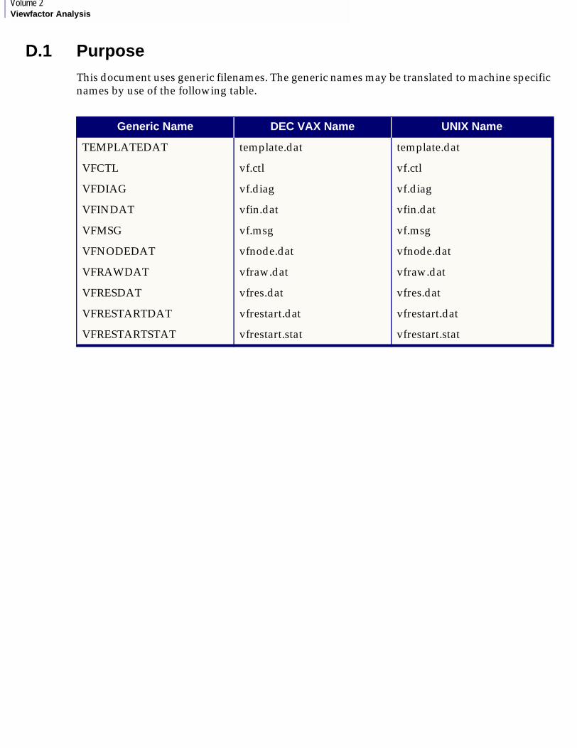
Volume 2Viewfactor Analysis
D.1 PurposeThis document uses generic filenames. The generic names may be translated to machine specific names by use of the following table.
Generic Name DEC VAX Name UNIX Name
TEMPLATEDAT template.dat template.dat
VFCTL vf.ctl vf.ctl
VFDIAG vf.diag vf.diag
VFINDAT vfin.dat vfin.dat
VFMSG vf.msg vf.msg
VFNODEDAT vfnode.dat vfnode.dat
VFRAWDAT vfraw.dat vfraw.dat
VFRESDAT vfres.dat vfres.dat
VFRESTARTDAT vfrestart.dat vfrestart.dat
VFRESTARTSTAT vfrestart.stat vfrestart.stat
MSC.Patran Thermal User’s Guide, Volume 2: Viewfactor Analysis
APPENDIX
E Example Thermal Radiation Problems
■ Purpose
■ Problem 1 - Steady-State Radiative Boundary Conditions
■ Problem 2 - Parallel Semi-Infinite Plates
■ Problem 3 - Heated Reaction Chamber

Volume 2Viewfactor Analysis
E.1 PurposeThese examples are simple problems designed to demonstrate the thermal radiation analysis process. The first example, steady-state radiative boundary conditions, is a two-enclosure radiative model. The second, parallel semi-infinite plates, is an idealized situation for which the correct thermal solution is known. The third example, more representative of a real world problem, models the interior of a reaction chamber.
In the first example, a step-by-step model definition is given, including figures showing the MSC.Patran forms. For the subsequent examples, to avoid repeating the forms, only the significant model data is given.
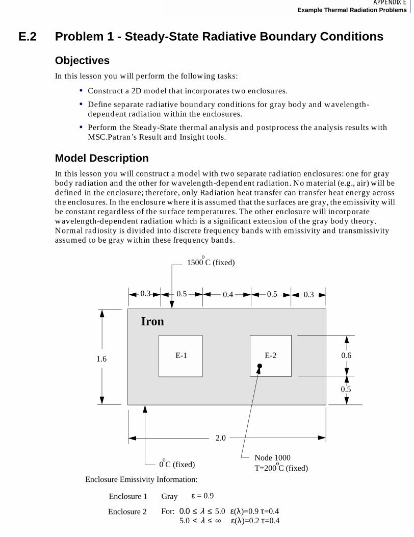
1APPENDIX EExample Thermal Radiation Problems
E.2 Problem 1 - Steady-State Radiative Boundary Conditions
ObjectivesIn this lesson you will perform the following tasks:
• Construct a 2D model that incorporates two enclosures.
• Define separate radiative boundary conditions for gray body and wavelength-dependent radiation within the enclosures.
• Perform the Steady-State thermal analysis and postprocess the analysis results with MSC.Patran’s Result and Insight tools.
Model DescriptionIn this lesson you will construct a model with two separate radiation enclosures: one for gray body radiation and the other for wavelength-dependent radiation. No material (e.g., air) will be defined in the enclosure; therefore, only Radiation heat transfer can transfer heat energy across the enclosures. In the enclosure where it is assumed that the surfaces are gray, the emissivity will be constant regardless of the surface temperatures. The other enclosure will incorporate wavelength-dependent radiation which is a significant extension of the gray body theory. Normal radiosity is divided into discrete frequency bands with emissivity and transmissivity assumed to be gray within these frequency bands.
1.6 E-1 E-2
2.0
Iron
0.6
0.5
0.3 0.5 0.4 0.5 0.3
Node 1000T=200 C (fixed)
o0 C (fixed)o
1500 C (fixed)o
Enclosure Emissivity Information:
Enclosure 1 Gray ε = 0.9
Enclosure 2 For: 0.0 λ 5.0≤ ≤ ε(λ)=0.9 τ=0.45.0 λ< ∞≤ ε(λ)=0.2 τ=0.4
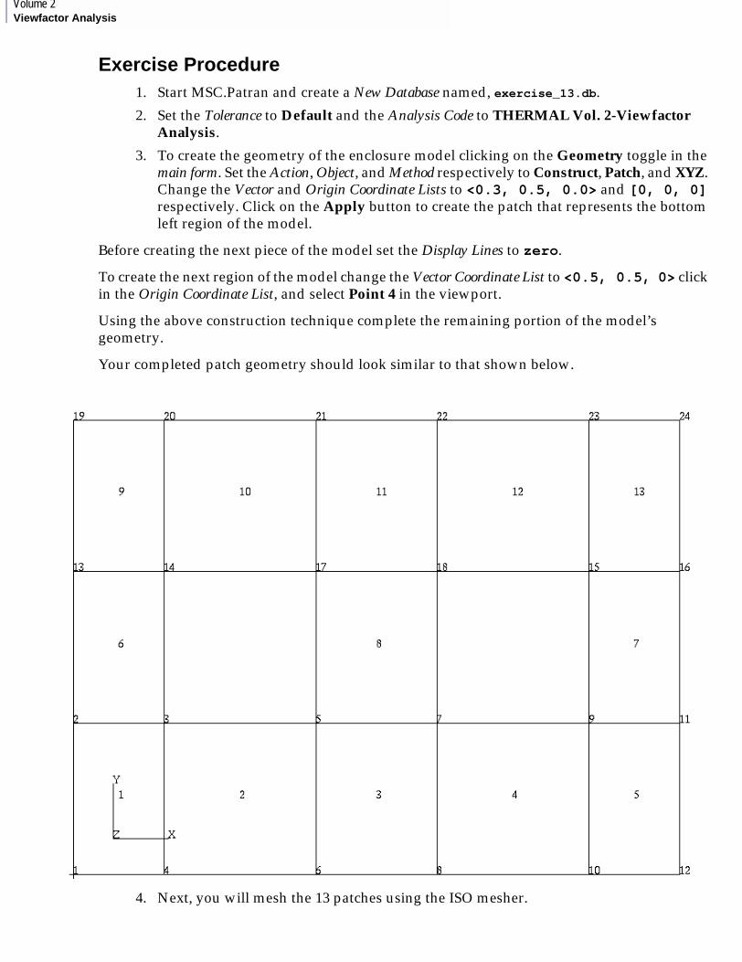
Volume 2Viewfactor Analysis
Exercise Procedure1. Start MSC.Patran and create a New Database named, exercise_13.db.
2. Set the Tolerance to Default and the Analysis Code to THERMAL Vol. 2-Viewfactor Analysis.
3. To create the geometry of the enclosure model clicking on the Geometry toggle in the main form. Set the Action, Object, and Method respectively to Construct, Patch, and XYZ. Change the Vector and Origin Coordinate Lists to <0.3, 0.5, 0.0> and [0, 0, 0] respectively. Click on the Apply button to create the patch that represents the bottom left region of the model.
Before creating the next piece of the model set the Display Lines to zero.
To create the next region of the model change the Vector Coordinate List to <0.5, 0.5, 0> click in the Origin Coordinate List, and select Point 4 in the viewport.
Using the above construction technique complete the remaining portion of the model’s geometry.
Your completed patch geometry should look similar to that shown below.
4. Next, you will mesh the 13 patches using the ISO mesher.
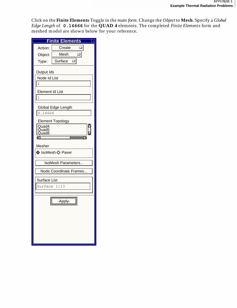
1APPENDIX EExample Thermal Radiation Problems
Click on the Finite Elements Toggle in the main form. Change the Object to Mesh. Specify a Global Edge Length of 0.16666 for the QUAD 4 elements. The completed Finite Elements form and meshed model are shown below for your reference.
Finite ElementsCreateAction:
MeshObject:
SurfaceType:
1
Node Id List
1
Element Id List
Output Ids
0.16666
Global Edge Length
Quad4Quad5Quad8
Element Topology
IsoMesh Paver
Mesher
IsoMesh Parameters...
Node Coordinate Frames...
Surface 1:13
Surface List
-Apply-

Volume 2Viewfactor Analysis
To simplify the visual image of your model, turn off all entity labels. Your model should now look like the one shown below.
5. To equivalence your model, change the Finite Element form’s Action, Object, and Type respectively to Equivalence, All, and Tolerance Cube. Click on the Apply button to equivalence the finite elements.
6. The model’s Enclosure 2 (hole on the right-hand side) will contain a medium that will participate in the radiation heat transfer occurring throughout that enclosure.
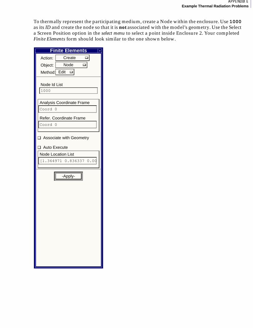
1APPENDIX EExample Thermal Radiation Problems
To thermally represent the participating medium, create a Node within the enclosure. Use 1000 as its ID and create the node so that it is not associated with the model’s geometry. Use the Select a Screen Position option in the select menu to select a point inside Enclosure 2. Your completed Finite Elements form should look similar to the one shown below.
Finite ElementsCreateAction:
NodeObject:
EditMethod:
1000
Node Id List
Coord 0
Analysis Coordinate Frame
Coord 0
Refer. Coordinate Frame
Associate with Geometry
[1.364971 0.836337 0.00
Node Location List
Auto Execute
-Apply-

Volume 2Viewfactor Analysis
To better visualize the Node locations, set their radius to 6 pixels. Your model should now look like the one shown below.
7. You will now create the required boundary conditions for your model.
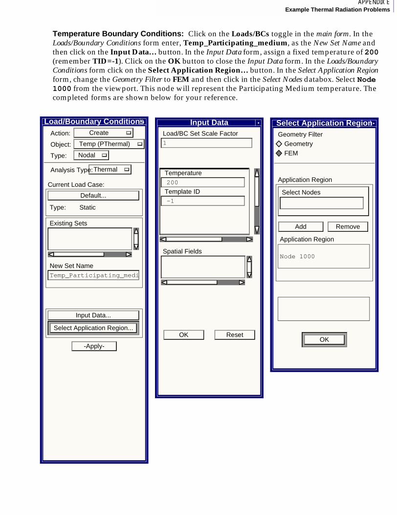
1APPENDIX EExample Thermal Radiation Problems
Temperature Boundary Conditions: Click on the Loads/BCs toggle in the main form. In the Loads/Boundary Conditions form enter, Temp_Participating_medium, as the New Set Name and then click on the Input Data… button. In the Input Data form, assign a fixed temperature of 200 (remember TID=-1). Click on the OK button to close the Input Data form. In the Loads/Boundary Conditions form click on the Select Application Region… button. In the Select Application Region form, change the Geometry Filter to FEM and then click in the Select Nodes databox. Select Node 1000 from the viewport. This node will represent the Participating Medium temperature. The completed forms are shown below for your reference.
Load/Boundary ConditionsCreateAction:
ThermalAnalysis Type:
Temp (PThermal)Object:
NodalType:
Default...
Type: Static
Current Load Case:
Existing Sets
Temp_Participating_medi
New Set Name
Input Data...
Select Application Region...
-Apply-
Input Data
1
Load/BC Set Scale Factor
200
Temperature
-1
Template ID
Spatial Fields
OK Reset
Select Application Region
Geometry
FEM
Geometry Filter
Select Nodes
Add Remove
Application Region
Node 1000
Application Region
OK
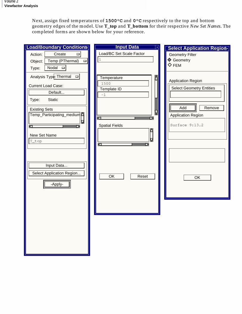
Volume 2Viewfactor Analysis
Next, assign fixed temperatures of 1500°C and 0°C respectively to the top and bottom geometry edges of the model. Use T_top and T_bottom for their respective New Set Names. The completed forms are shown below for your reference.
Input Data
1
Load/BC Set Scale Factor
1500
Temperature
-1
Template ID
Spatial Fields
OK Reset
Select Application Region
GeometryFEM
Geometry Filter
Select Geometry Entities
Add Remove
Application Region
Surface 9:13.2
Application Region
OK
Load/Boundary ConditionsCreateAction:
ThermalAnalysis Type:
Temp (PThermal)Object:
NodalType:
Default...
Type: Static
Current Load Case:
Existing SetsTemp_Participating_medium
T_top
New Set Name
Input Data...
Select Application Region...
-Apply-
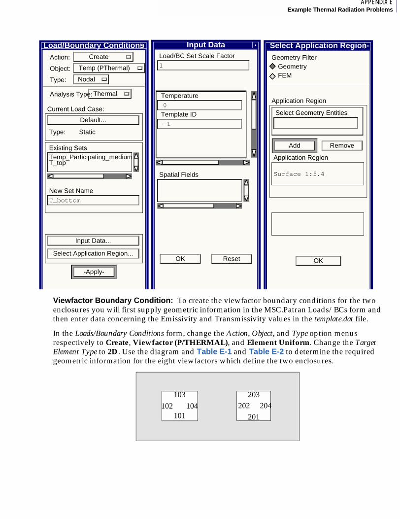
1APPENDIX EExample Thermal Radiation Problems
Viewfactor Boundary Condition: To create the viewfactor boundary conditions for the two enclosures you will first supply geometric information in the MSC.Patran Loads/BCs form and then enter data concerning the Emissivity and Transmissivity values in the template.dat file.
In the Loads/Boundary Conditions form, change the Action, Object, and Type option menus respectively to Create, Viewfactor (P/THERMAL), and Element Uniform. Change the Target Element Type to 2D. Use the diagram and Table E-1 and Table E-2 to determine the required geometric information for the eight viewfactors which define the two enclosures.
Input Data
1
Load/BC Set Scale Factor
0
Temperature
-1
Template ID
Spatial Fields
OK Reset
Load/Boundary ConditionsCreateAction:
ThermalAnalysis Type:
Temp (PThermal)Object:
NodalType:
Default...
Type: Static
Current Load Case:
Existing SetsTemp_Participating_mediumT_top
T_bottom
New Set Name
Input Data...
Select Application Region...
-Apply-
Select Application Region
GeometryFEM
Geometry Filter
Select Geometry Entities
Add Remove
Application Region
Surface 1:5.4
Application Region
OK
203
202
201
204101
102
103
104
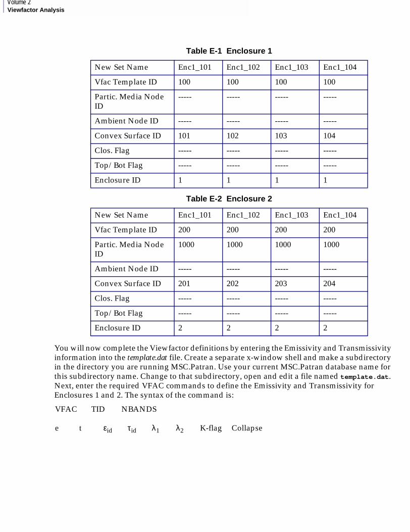
Volume 2Viewfactor Analysis
You will now complete the Viewfactor definitions by entering the Emissivity and Transmissivity information into the template.dat file. Create a separate x-window shell and make a subdirectory in the directory you are running MSC.Patran. Use your current MSC.Patran database name for this subdirectory name. Change to that subdirectory, open and edit a file named template.dat. Next, enter the required VFAC commands to define the Emissivity and Transmissivity for Enclosures 1 and 2. The syntax of the command is:
Table E-1 Enclosure 1
New Set Name Enc1_101 Enc1_102 Enc1_103 Enc1_104
Vfac Template ID 100 100 100 100
Partic. Media Node ID
----- ----- ----- -----
Ambient Node ID ----- ----- ----- -----
Convex Surface ID 101 102 103 104
Clos. Flag ----- ----- ----- -----
Top/Bot Flag ----- ----- ----- -----
Enclosure ID 1 1 1 1
Table E-2 Enclosure 2
New Set Name Enc1_101 Enc1_102 Enc1_103 Enc1_104
Vfac Template ID 200 200 200 200
Partic. Media Node ID
1000 1000 1000 1000
Ambient Node ID ----- ----- ----- -----
Convex Surface ID 201 202 203 204
Clos. Flag ----- ----- ----- -----
Top/Bot Flag ----- ----- ----- -----
Enclosure ID 2 2 2 2
VFAC TID NBANDS
e t εid τid λ1 λ2 K-flag Collapse
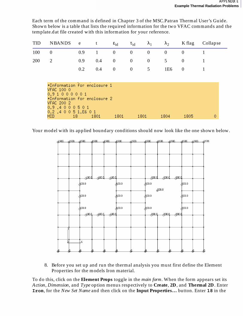
1APPENDIX EExample Thermal Radiation Problems
Each term of the command is defined in Chapter 3 of the MSC.Patran Thermal User’s Guide. Shown below is a table that lists the required information for the two VFAC commands and the template.dat file created with this information for your reference.
Your model with its applied boundary conditions should now look like the one shown below.
8. Before you set up and run the thermal analysis you must first define the Element Properties for the models Iron material.
To do this, click on the Element Props toggle in the main form. When the form appears set its Action, Dimension, and Type option menus respectively to Create, 2D, and Thermal 2D. Enter Iron, for the New Set Name and then click on the Input Properties… button. Enter 18 in the
TID NBANDS e t εid τid λ1 λ2 K flag Collapse
100 0 0.9 1 0 0 0 0 0 1
200 2 0.9 0.4 0 0 0 5 0 1
0.2 0.4 0 0 5 1E6 0 1
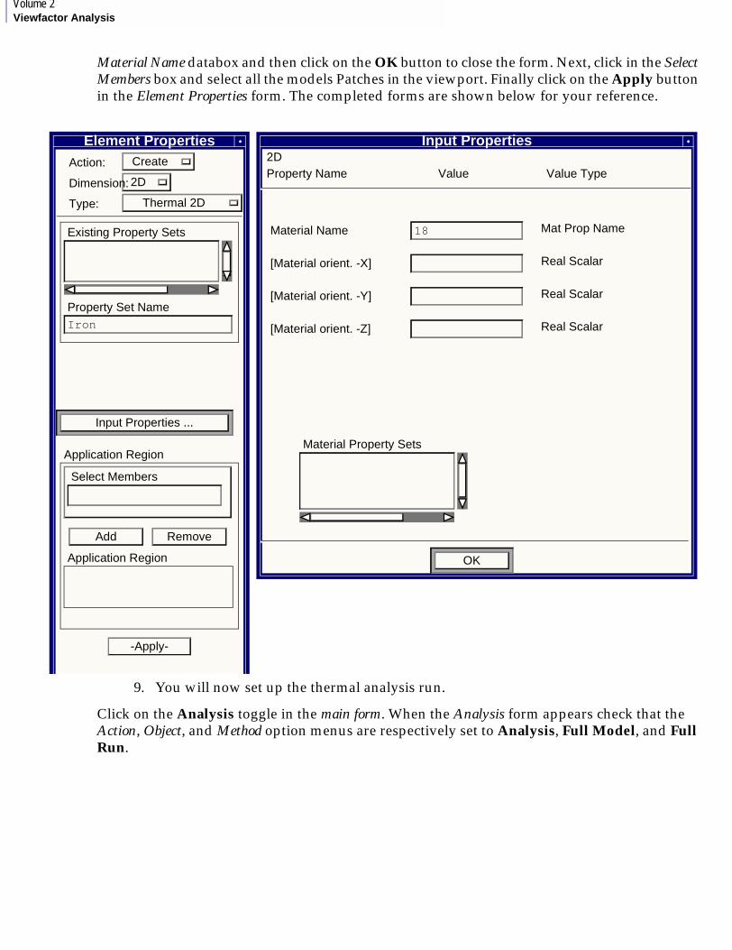
Volume 2Viewfactor Analysis
Material Name databox and then click on the OK button to close the form. Next, click in the Select Members box and select all the models Patches in the viewport. Finally click on the Apply button in the Element Properties form. The completed forms are shown below for your reference.
9. You will now set up the thermal analysis run.
Click on the Analysis toggle in the main form. When the Analysis form appears check that the Action, Object, and Method option menus are respectively set to Analysis, Full Model, and Full Run.
Element PropertiesCreateAction:
2DDimension:
Thermal 2DType:
Existing Property Sets
Iron
Property Set Name
Input Properties ...
Select Members
Add Remove
Application Region
Application Region
-Apply-
Input Properties2DProperty Name Value Value Type
Mat Prop Name18Material Name
Real Scalar[Material orient. -X]
Real Scalar[Material orient. -Y]
Real Scalar[Material orient. -Z]
Material Property Sets
OK
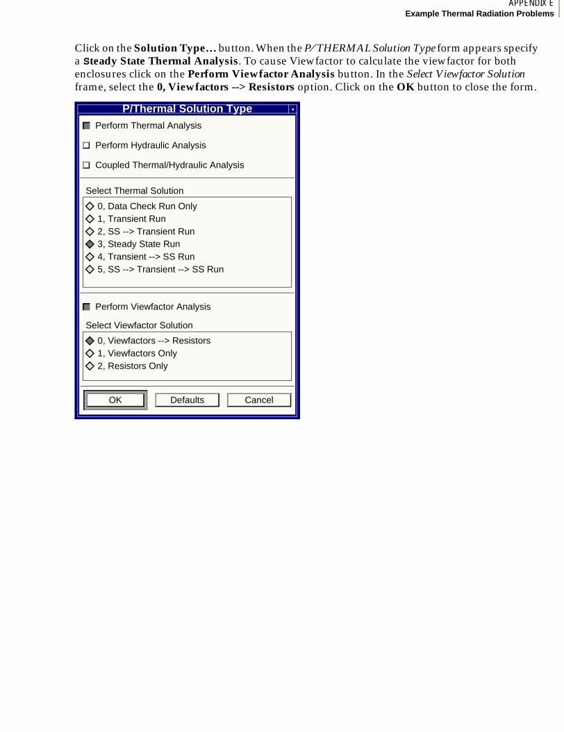
1APPENDIX EExample Thermal Radiation Problems
Click on the Solution Type… button. When the P⁄ THERMAL Solution Type form appears specify a Steady State Thermal Analysis. To cause Viewfactor to calculate the viewfactor for both enclosures click on the Perform Viewfactor Analysis button. In the Select Viewfactor Solution frame, select the 0, Viewfactors --> Resistors option. Click on the OK button to close the form.
P/Thermal Solution TypePerform Thermal Analysis
Perform Hydraulic Analysis
Coupled Thermal/Hydraulic Analysis
0, Data Check Run Only1, Transient Run2, SS --> Transient Run3, Steady State Run4, Transient --> SS Run5, SS --> Transient --> SS Run
Select Thermal Solution
Perform Viewfactor Analysis
0, Viewfactors --> Resistors1, Viewfactors Only2, Resistors Only
Select Viewfactor Solution
OK Defaults Cancel
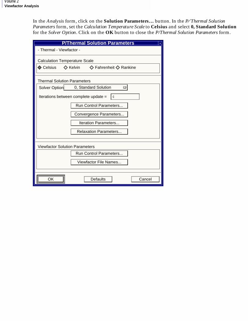
Volume 2Viewfactor Analysis
In the Analysis form, click on the Solution Parameters… button. In the P⁄ Thermal Solution Parameters form, set the Calculation Temperature Scale to Celsius and select 0, Standard Solution for the Solver Option. Click on the OK button to close the P/Thermal Solution Parameters form.
P/Thermal Solution Parameters- Thermal - Viewfactor -
Celsius Kelvin Fahrenheit Rankine
Calculation Temperature Scale
0, Standard SolutionSolver Option:
4Iterations between complete update =
Run Control Parameters...
Convergence Parameters...
Iteration Parameters...
Relaxation Parameters...
Thermal Solution Parameters
Run Control Parameters...
Viewfactor File Names...
Viewfactor Solution Parameters
OK Defaults Cancel
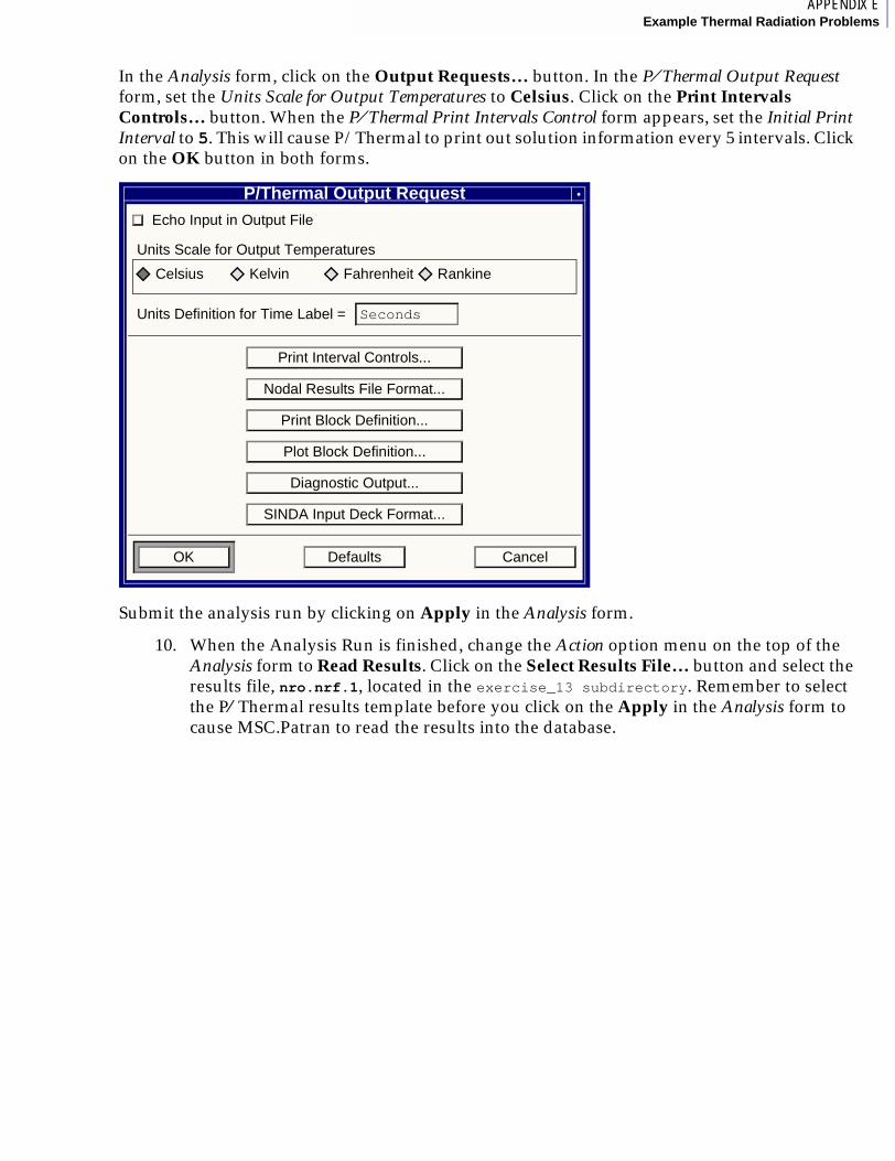
1APPENDIX EExample Thermal Radiation Problems
In the Analysis form, click on the Output Requests… button. In the P⁄ Thermal Output Request form, set the Units Scale for Output Temperatures to Celsius. Click on the Print Intervals Controls… button. When the P⁄ Thermal Print Intervals Control form appears, set the Initial Print Interval to 5. This will cause P/Thermal to print out solution information every 5 intervals. Click on the OK button in both forms.
Submit the analysis run by clicking on Apply in the Analysis form.
10. When the Analysis Run is finished, change the Action option menu on the top of the Analysis form to Read Results. Click on the Select Results File… button and select the results file, nro.nrf.1, located in the exercise_13 subdirectory. Remember to select the P⁄ Thermal results template before you click on the Apply in the Analysis form to cause MSC.Patran to read the results into the database.
P/Thermal Output RequestEcho Input in Output File
Celsius Kelvin Fahrenheit Rankine
Units Scale for Output Temperatures
SecondsUnits Definition for Time Label =
Print Interval Controls...
Nodal Results File Format...
Print Block Definition...
Plot Block Definition...
Diagnostic Output...
SINDA Input Deck Format...
OK Defaults Cancel
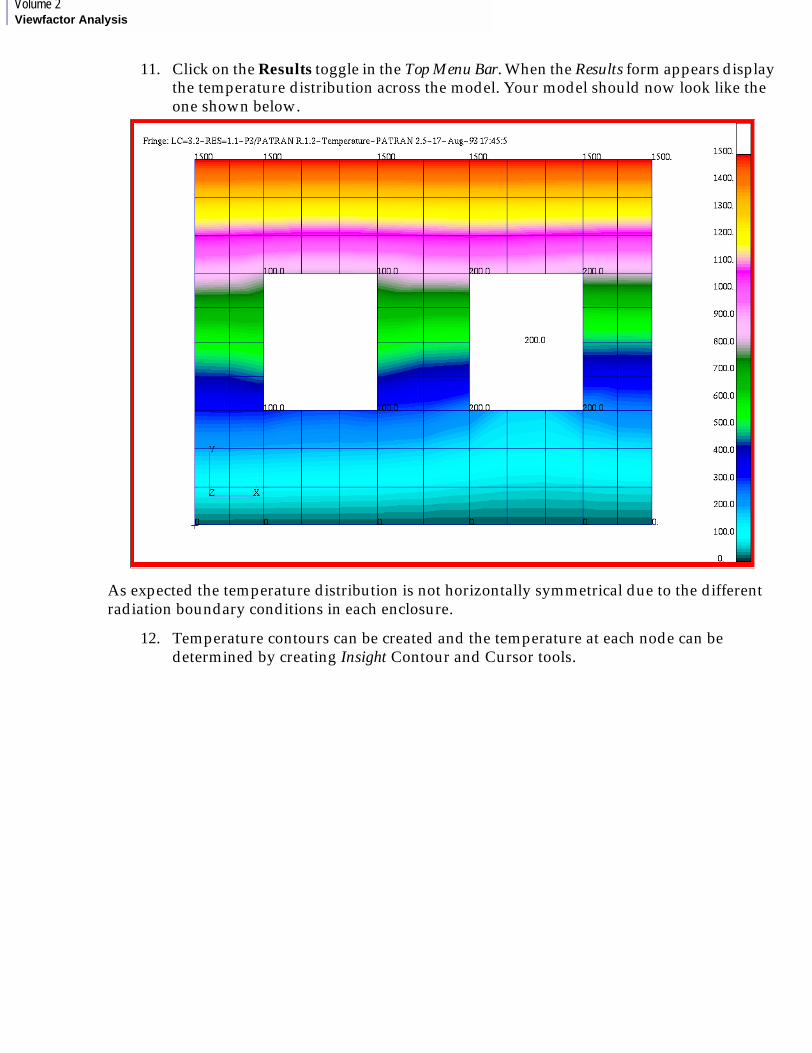
Volume 2Viewfactor Analysis
11. Click on the Results toggle in the Top Menu Bar. When the Results form appears display the temperature distribution across the model. Your model should now look like the one shown below.
As expected the temperature distribution is not horizontally symmetrical due to the different radiation boundary conditions in each enclosure.
12. Temperature contours can be created and the temperature at each node can be determined by creating Insight Contour and Cursor tools.
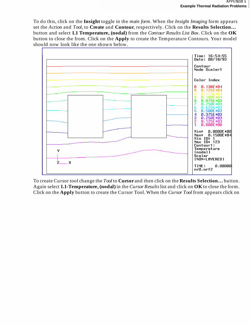
1APPENDIX EExample Thermal Radiation Problems
To do this, click on the Insight toggle in the main form. When the Insight Imaging form appears set the Action and Tool, to Create and Contour, respectively. Click on the Results Selection… button and select 1.1 Temperature, (nodal) from the Contour Results List Box. Click on the OK button to close the from. Click on the Apply to create the Temperature Contours. Your model should now look like the one shown below.
To create Cursor tool change the Tool to Cursor and then click on the Results Selection… button. Again select 1.1-Temperature, (nodal) in the Cursor Results list and click on OK to close the form. Click on the Apply button to create the Cursor Tool. When the Cursor Tool from appears click on
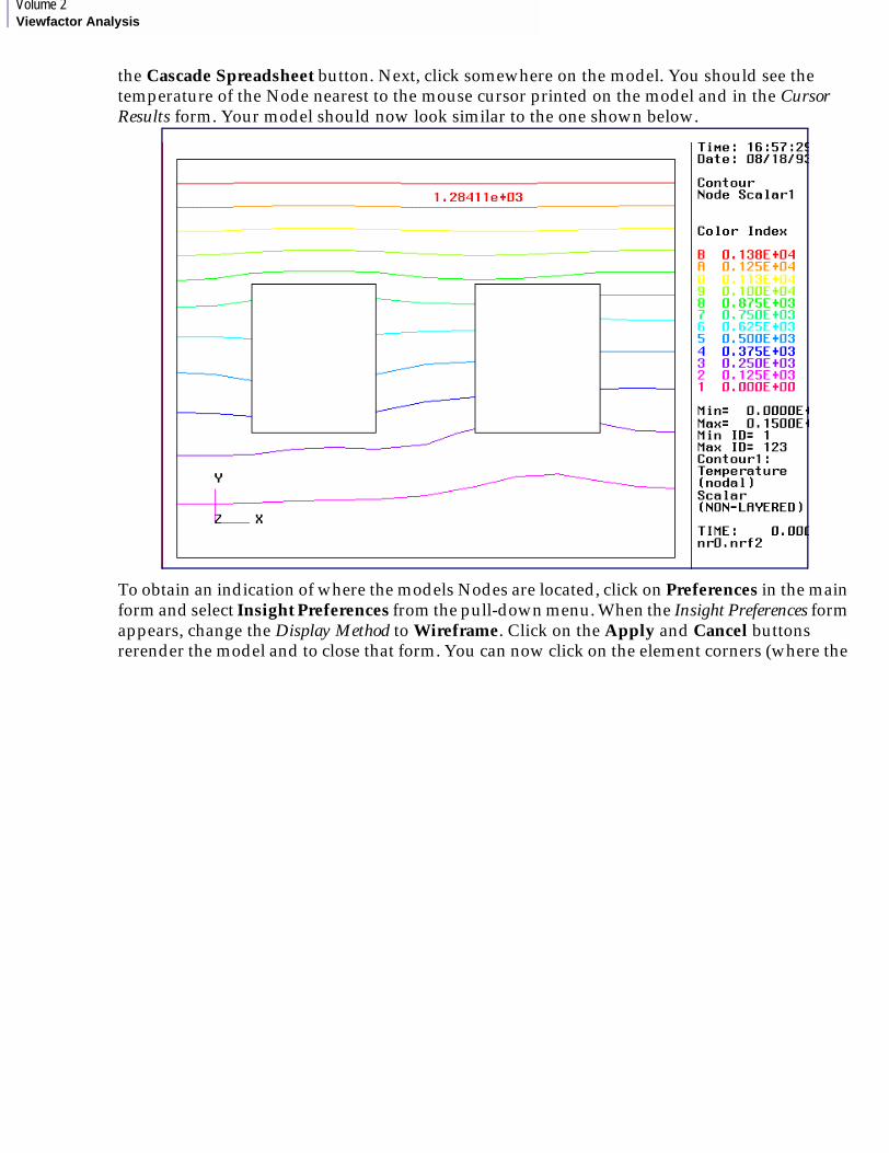
Volume 2Viewfactor Analysis
the Cascade Spreadsheet button. Next, click somewhere on the model. You should see the temperature of the Node nearest to the mouse cursor printed on the model and in the Cursor Results form. Your model should now look similar to the one shown below.
To obtain an indication of where the models Nodes are located, click on Preferences in the main form and select Insight Preferences from the pull-down menu. When the Insight Preferences form appears, change the Display Method to Wireframe. Click on the Apply and Cancel buttons rerender the model and to close that form. You can now click on the element corners (where the
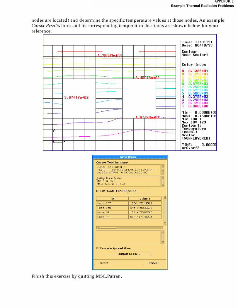
1APPENDIX EExample Thermal Radiation Problems
nodes are located) and determine the specific temperature values at those nodes. An example Cursor Results form and its corresponding temperature locations are shown below for your reference.
Finish this exercise by quitting MSC.Patran.
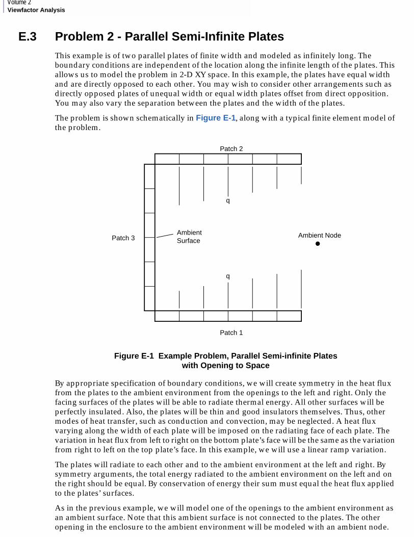
Volume 2Viewfactor Analysis
E.3 Problem 2 - Parallel Semi-Infinite PlatesThis example is of two parallel plates of finite width and modeled as infinitely long. The boundary conditions are independent of the location along the infinite length of the plates. This allows us to model the problem in 2-D XY space. In this example, the plates have equal width and are directly opposed to each other. You may wish to consider other arrangements such as directly opposed plates of unequal width or equal width plates offset from direct opposition. You may also vary the separation between the plates and the width of the plates.
The problem is shown schematically in Figure E-1, along with a typical finite element model of the problem.
Figure E-1 Example Problem, Parallel Semi-infinite Plates with Opening to Space
By appropriate specification of boundary conditions, we will create symmetry in the heat flux from the plates to the ambient environment from the openings to the left and right. Only the facing surfaces of the plates will be able to radiate thermal energy. All other surfaces will be perfectly insulated. Also, the plates will be thin and good insulators themselves. Thus, other modes of heat transfer, such as conduction and convection, may be neglected. A heat flux varying along the width of each plate will be imposed on the radiating face of each plate. The variation in heat flux from left to right on the bottom plate’s face will be the same as the variation from right to left on the top plate’s face. In this example, we will use a linear ramp variation.
The plates will radiate to each other and to the ambient environment at the left and right. By symmetry arguments, the total energy radiated to the ambient environment on the left and on the right should be equal. By conservation of energy their sum must equal the heat flux applied to the plates’ surfaces.
As in the previous example, we will model one of the openings to the ambient environment as an ambient surface. Note that this ambient surface is not connected to the plates. The other opening in the enclosure to the ambient environment will be modeled with an ambient node.
AmbientSurface
Ambient NodePatch 3
Patch 2
Patch 1
q
q
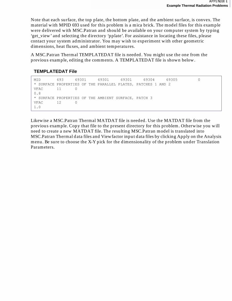
2APPENDIX EExample Thermal Radiation Problems
Note that each surface, the top plate, the bottom plate, and the ambient surface, is convex. The material with MPID 693 used for this problem is a mica brick. The model files for this example were delivered with MSC.Patran and should be available on your computer system by typing ‘get_view’ and selecting the directory ‘pplate’. For assistance in locating these files, please contact your system administrator. You may wish to experiment with other geometric dimensions, heat fluxes, and ambient temperatures.
A MSC.Patran Thermal TEMPLATEDAT file is needed. You might use the one from the previous example, editing the comments. A TEMPLATEDAT file is shown below.
Likewise a MSC.Patran Thermal MATDAT file is needed. Use the MATDAT file from the previous example. Copy that file to the present directory for this problem. Otherwise you will need to create a new MATDAT file. The resulting MSC.Patran model is translated into MSC.Patran Thermal data files and Viewfactor input data files by clicking Apply on the Analysis menu. Be sure to choose the X-Y pick for the dimensionality of the problem under Translation Parameters.
TEMPLATEDAT File
MID 693 69301 69301 69301 69304 69305 0 * SURFACE PROPERTIES OF THE PARALLEL PLATES, PATCHES 1 AND 2VFAC 11 00.8* SURFACE PROPERTIES OF THE AMBIENT SURFACE, PATCH 3VFAC 12 01.0
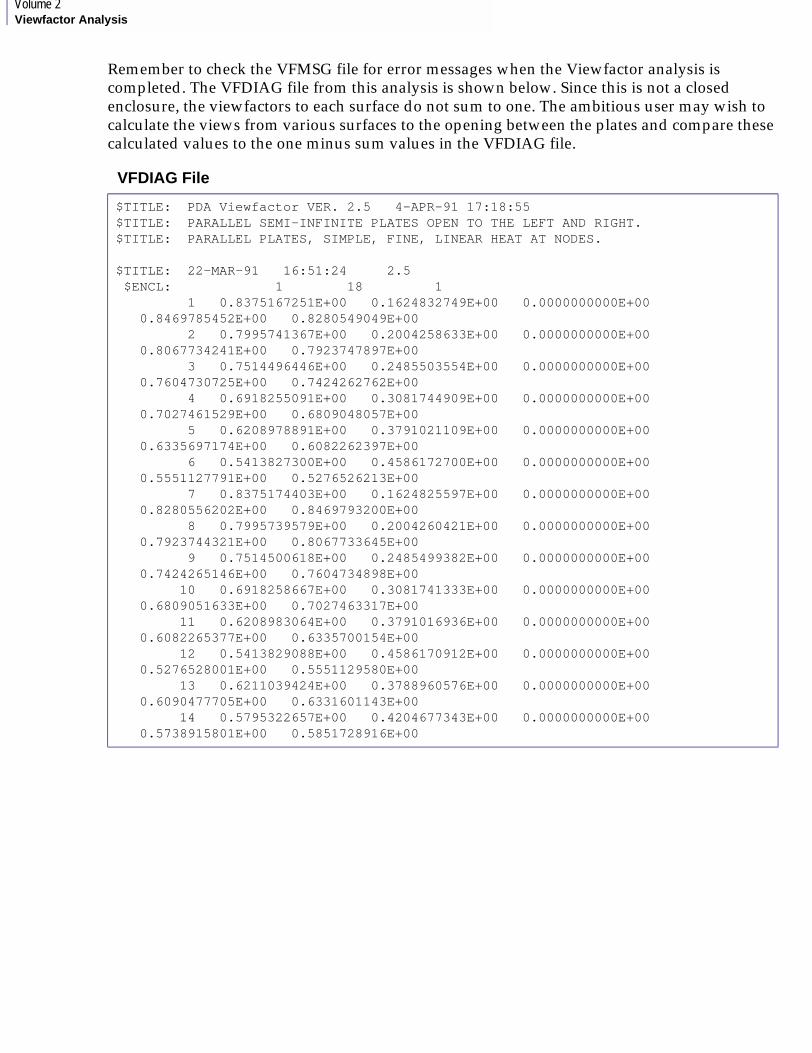
Volume 2Viewfactor Analysis
Remember to check the VFMSG file for error messages when the Viewfactor analysis is completed. The VFDIAG file from this analysis is shown below. Since this is not a closed enclosure, the viewfactors to each surface do not sum to one. The ambitious user may wish to calculate the views from various surfaces to the opening between the plates and compare these calculated values to the one minus sum values in the VFDIAG file.
VFDIAG File
$TITLE: PDA Viewfactor VER. 2.5 4-APR-91 17:18:55 $TITLE: PARALLEL SEMI-INFINITE PLATES OPEN TO THE LEFT AND RIGHT. $TITLE: PARALLEL PLATES, SIMPLE, FINE, LINEAR HEAT AT NODES. $TITLE: 22-MAR-91 16:51:24 2.5 $ENCL: 1 18 1 1 0.8375167251E+00 0.1624832749E+00 0.0000000000E+00 0.8469785452E+00 0.8280549049E+00 2 0.7995741367E+00 0.2004258633E+00 0.0000000000E+00 0.8067734241E+00 0.7923747897E+00 3 0.7514496446E+00 0.2485503554E+00 0.0000000000E+00 0.7604730725E+00 0.7424262762E+00 4 0.6918255091E+00 0.3081744909E+00 0.0000000000E+00 0.7027461529E+00 0.6809048057E+00 5 0.6208978891E+00 0.3791021109E+00 0.0000000000E+00 0.6335697174E+00 0.6082262397E+00 6 0.5413827300E+00 0.4586172700E+00 0.0000000000E+00 0.5551127791E+00 0.5276526213E+00 7 0.8375174403E+00 0.1624825597E+00 0.0000000000E+00 0.8280556202E+00 0.8469793200E+00 8 0.7995739579E+00 0.2004260421E+00 0.0000000000E+00 0.7923744321E+00 0.8067733645E+00 9 0.7514500618E+00 0.2485499382E+00 0.0000000000E+00 0.7424265146E+00 0.7604734898E+00 10 0.6918258667E+00 0.3081741333E+00 0.0000000000E+00 0.6809051633E+00 0.7027463317E+00 11 0.6208983064E+00 0.3791016936E+00 0.0000000000E+00 0.6082265377E+00 0.6335700154E+00 12 0.5413829088E+00 0.4586170912E+00 0.0000000000E+00 0.5276528001E+00 0.5551129580E+00 13 0.6211039424E+00 0.3788960576E+00 0.0000000000E+00 0.6090477705E+00 0.6331601143E+00 14 0.5795322657E+00 0.4204677343E+00 0.0000000000E+00 0.5738915801E+00 0.5851728916E+00

2APPENDIX EExample Thermal Radiation Problems
$QTRAN
Finally, you will want to look at the MSC.Patran Thermal output data in the QOUTDAT file. Use the system editor to find the first occurrence of the string '1TIME'. Note the system heat balance. This is approximately the imposed heat flux to the plates’ surfaces. Page down through the data to node 1000, the ambient node. Note that the heat flux at this node is approximately half of the imposed heat flux as expected. Sum up the heat fluxes to the ambient surface and note that this sum is approximately half of the imposed total heat flux. The nodes numbered above 1000 are the radiosity nodes created by Viewfactor.
This is a simple problem and you may wish to try numerous variations on it, such as refining the mesh, changing the convergence criteria, changing the double area parameter of the $GAUSS_ORDER, changing the imposed heat flux, changing the ambient environment temperature, specifying the plate surface temperatures, and entering more complicated descriptions of the radiative surface properties.
15 0.5567277074E+00 0.4432722926E+00 0.0000000000E+00 0.5546888113E+00 0.5587666035E+00 16 0.5567269325E+00 0.4432730675E+00 0.0000000000E+00 0.5587658286E+00 0.5546880364E+00 17 0.5795311928E+00 0.4204688072E+00 0.0000000000E+00 0.5851718783E+00 0.5738904476E+00 18 0.6211042404E+00 0.3788957596E+00 0.0000000000E+00 0.6331602335E+00 0.6090482473E+00 0.4586173E+00 0.3333322E+00 0.1052847E+00 0.3333322E+00 0.1052847E+00 0.4723472E+00 0.3333322E+00 0.1057708E+00 0.3333322E+00 0.1057708E+00 0.4723474E+00 0.3333322E+00 0.1057709E+00 0.3333322E+00 0.1057709E+00 $ENDENCL: $EOF:

Volume 2Viewfactor Analysis
E.4 Problem 3 - Heated Reaction ChamberThis example represents a simple version of a reaction chamber. The main chamber is a short vertical cylinder with hemispherical caps on each end. The main chamber also has a smaller chamber teed off from its side. The smaller chamber is a short cylinder, with a smaller diameter than the large chamber, and capped with a hemispherical cap. The chamber walls are constructed of a high-strength steel which corresponds to material ID 365 in the material property database provided with the MSC.Patran Thermal module. The model was created using the MKS system of units for the physical and material properties.
The bottom cap of the main chamber is heated with a flux of 5000 watts per square meter applied to the exterior surface. The rest of the exterior surface is convectively coupled to the ambient environment at 300 K. The convection coefficients are constant with the value for the main chamber being 1 watt per square meter per degree K and the value for the smaller chamber being 20.
The interior of the chamber has only thermal radiation boundary conditions. A participating media node is included in the model in case we wish to use it in the future. However, it is not used in the analysis presented here.
The MSC.Patran model uses a very coarse mesh, since we do not want to use up a large amount of computer time on an example problem. The model files for this example were delivered with MSC.Patran Thermal and should be available on your computer system by typing ‘get_view’ and selecting the directory ‘chamber.’ For assistance in locating these files, please contact your system administrator.
A MSC.Patran Thermal TEMPLATEDAT file is needed. A TEMPLATEDAT file is shown below.
The material template ID 365 is for the high-strength steel used for the vessel walls and the VFAC template 365 is for the interior surfaces of the vessel. The template gives the emissivity as a constant value of 0.8. No other radiation property data is given in this case since this is a simple model.
TEMPLATEDAT File
MID 365 36501 36501 36501 36504 36505 36506 *VFAC 365 00.8 1.0 0 0 0 0 0 1
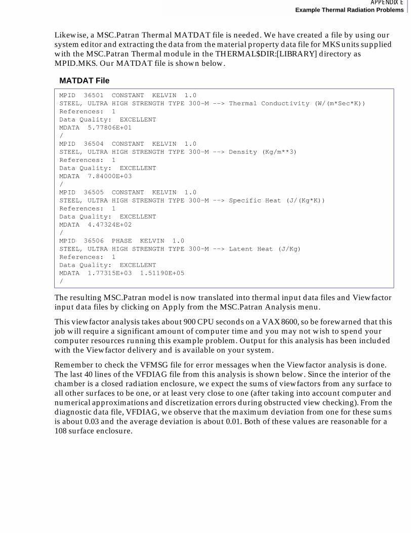
2APPENDIX EExample Thermal Radiation Problems
Likewise, a MSC.Patran Thermal MATDAT file is needed. We have created a file by using our system editor and extracting the data from the material property data file for MKS units supplied with the MSC.Patran Thermal module in the THERMAL$DIR:[LIBRARY] directory as MPID.MKS. Our MATDAT file is shown below.
The resulting MSC.Patran model is now translated into thermal input data files and Viewfactor input data files by clicking on Apply from the MSC.Patran Analysis menu.
This viewfactor analysis takes about 900 CPU seconds on a VAX 8600, so be forewarned that this job will require a significant amount of computer time and you may not wish to spend your computer resources running this example problem. Output for this analysis has been included with the Viewfactor delivery and is available on your system.
Remember to check the VFMSG file for error messages when the Viewfactor analysis is done. The last 40 lines of the VFDIAG file from this analysis is shown below. Since the interior of the chamber is a closed radiation enclosure, we expect the sums of viewfactors from any surface to all other surfaces to be one, or at least very close to one (after taking into account computer and numerical approximations and discretization errors during obstructed view checking). From the diagnostic data file, VFDIAG, we observe that the maximum deviation from one for these sums is about 0.03 and the average deviation is about 0.01. Both of these values are reasonable for a 108 surface enclosure.
MATDAT File
MPID 36501 CONSTANT KELVIN 1.0STEEL, ULTRA HIGH STRENGTH TYPE 300-M --> Thermal Conductivity (W/(m*Sec*K))References: 1Data Quality: EXCELLENTMDATA 5.77806E+01/MPID 36504 CONSTANT KELVIN 1.0STEEL, ULTRA HIGH STRENGTH TYPE 300-M --> Density (Kg/m**3)References: 1Data Quality: EXCELLENTMDATA 7.84000E+03/MPID 36505 CONSTANT KELVIN 1.0STEEL, ULTRA HIGH STRENGTH TYPE 300-M --> Specific Heat (J/(Kg*K))References: 1Data Quality: EXCELLENTMDATA 4.47324E+02/MPID 36506 PHASE KELVIN 1.0STEEL, ULTRA HIGH STRENGTH TYPE 300-M --> Latent Heat (J/Kg)References: 1Data Quality: EXCELLENTMDATA 1.77315E+03 1.51190E+05/
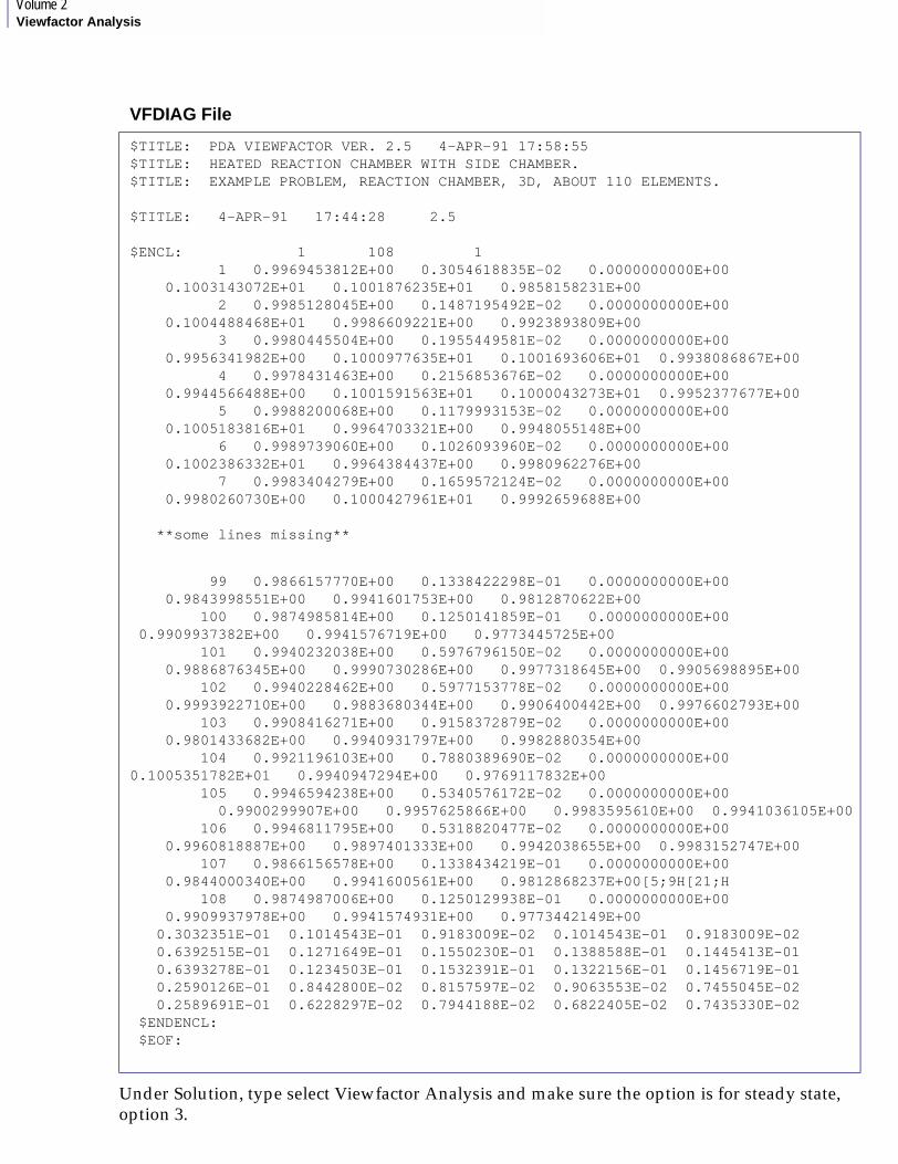
Volume 2Viewfactor Analysis
Under Solution, type select Viewfactor Analysis and make sure the option is for steady state, option 3.
VFDIAG File
$TITLE: PDA VIEWFACTOR VER. 2.5 4-APR-91 17:58:55 $TITLE: HEATED REACTION CHAMBER WITH SIDE CHAMBER.$TITLE: EXAMPLE PROBLEM, REACTION CHAMBER, 3D, ABOUT 110 ELEMENTS.
$TITLE: 4-APR-91 17:44:28 2.5 $ENCL: 1 108 1 1 0.9969453812E+00 0.3054618835E-02 0.0000000000E+00 0.1003143072E+01 0.1001876235E+01 0.9858158231E+00 2 0.9985128045E+00 0.1487195492E-02 0.0000000000E+00 0.1004488468E+01 0.9986609221E+00 0.9923893809E+00 3 0.9980445504E+00 0.1955449581E-02 0.0000000000E+00 0.9956341982E+00 0.1000977635E+01 0.1001693606E+01 0.9938086867E+00 4 0.9978431463E+00 0.2156853676E-02 0.0000000000E+00 0.9944566488E+00 0.1001591563E+01 0.1000043273E+01 0.9952377677E+00 5 0.9988200068E+00 0.1179993153E-02 0.0000000000E+00 0.1005183816E+01 0.9964703321E+00 0.9948055148E+00 6 0.9989739060E+00 0.1026093960E-02 0.0000000000E+00 0.1002386332E+01 0.9964384437E+00 0.9980962276E+00 7 0.9983404279E+00 0.1659572124E-02 0.0000000000E+00 0.9980260730E+00 0.1000427961E+01 0.9992659688E+00
**some lines missing**
99 0.9866157770E+00 0.1338422298E-01 0.0000000000E+00 0.9843998551E+00 0.9941601753E+00 0.9812870622E+00 100 0.9874985814E+00 0.1250141859E-01 0.0000000000E+00 0.9909937382E+00 0.9941576719E+00 0.9773445725E+00 101 0.9940232038E+00 0.5976796150E-02 0.0000000000E+00 0.9886876345E+00 0.9990730286E+00 0.9977318645E+00 0.9905698895E+00 102 0.9940228462E+00 0.5977153778E-02 0.0000000000E+00 0.9993922710E+00 0.9883680344E+00 0.9906400442E+00 0.9976602793E+00 103 0.9908416271E+00 0.9158372879E-02 0.0000000000E+00 0.9801433682E+00 0.9940931797E+00 0.9982880354E+00 104 0.9921196103E+00 0.7880389690E-02 0.0000000000E+000.1005351782E+01 0.9940947294E+00 0.9769117832E+00 105 0.9946594238E+00 0.5340576172E-02 0.0000000000E+00 0.9900299907E+00 0.9957625866E+00 0.9983595610E+00 0.9941036105E+00 106 0.9946811795E+00 0.5318820477E-02 0.0000000000E+00 0.9960818887E+00 0.9897401333E+00 0.9942038655E+00 0.9983152747E+00 107 0.9866156578E+00 0.1338434219E-01 0.0000000000E+00 0.9844000340E+00 0.9941600561E+00 0.9812868237E+00[5;9H[21;H 108 0.9874987006E+00 0.1250129938E-01 0.0000000000E+00 0.9909937978E+00 0.9941574931E+00 0.9773442149E+00 0.3032351E-01 0.1014543E-01 0.9183009E-02 0.1014543E-01 0.9183009E-02 0.6392515E-01 0.1271649E-01 0.1550230E-01 0.1388588E-01 0.1445413E-01 0.6393278E-01 0.1234503E-01 0.1532391E-01 0.1322156E-01 0.1456719E-01 0.2590126E-01 0.8442800E-02 0.8157597E-02 0.9063553E-02 0.7455045E-02 0.2589691E-01 0.6228297E-02 0.7944188E-02 0.6822405E-02 0.7435330E-02 $ENDENCL: $EOF:

2APPENDIX EExample Thermal Radiation Problems
A few minor modifications need to be made to the MSC.Patran Analysis form.
Under Viewfactor Solution Parameters, change the title to: Viewfactor EXAMPLE PROBLEM CHAMBER.
Under Solution Parameters, set EPSISS to1.0000000000d-03.
Under Output Requests, Diagnostic Output, set all of the toggles off, especially the radiation resistors to avoid receiving printout for tens of thousands of radiation resistors.
Under Solution Parameters, run control, set the initial temperature to 300 K.
The thermal analysis is spawned when Apply is selected on the Analysis menu. The analysis will take much longer than for a similar model without any radiative interchange. When the radiative interchange is modeled in this example, nearly every nodal subarea on the interior surface of the vessel is connected to nearly every other nodal subarea on the interior surface by means of radiation resistors. Thus the resistor network which QTRAN must solve has many times more resistors than a similar model without radiation coupling. Also, the heat transfer across the radiative resistors is highly nonlinear. This further increases the time required for QTRAN to solve the network equations. The QTRAN thermal network analysis will require approximately 6000 CPU seconds on a VAX 8600.
You may not wish to spend your computer resources running this example problem. Output for this analysis has been included with the Viewfactor delivery and should be available on your system.
When the analysis is done, the following results may be read into the MSC.Patran database under the Analysis menu with the Action set to Read Results. The results can be visualized with any of the visualization tools under Results.
Finally, you will want to look at the MSC.Patran Thermal output data in the QOUTDAT file. Use the system editor to find the first occurrence of the string '1TIME'. Note the system heat balance. This is approximately the imposed heat flux to the chamber’s bottom cap. Also note that although the temperatures are converged to high accuracy, the total system heat balance is not nearly so accurate. This illustrates the significance of the fourth power temperature dependence for radiant energy exchange. If accurate heat flows are required for a thermal analysis of a high temperature radiation environment, then very accurate temperatures must in general be calculated. The nodes numbered above 2000 are the radiosity nodes created by Viewfactor.

Volume 2Viewfactor Analysis
2
I N D E XMSC.Patran Thermal User’s Guide Volume 2: Viewfactor Analysis
I N D E XMSC.Patran Thermal User’s Guide
Volume 2: Viewfactor Analysis
Symbols$APPROX_CURVE, 104$AXISYM_SURFACE, 105$CONVERGE, 102$DIAGNOSTIC_FILE, 99$ENDNODES, 148$ENDSYM, 146$EOF, 106$GAUSS_ORDER, 104$IN_DATA, 100$MESSAGE_FILE, 99$NODES, 148$OUT_DATA, 100$PATH, 98$RAD_NODE_FILE, 101$RAW_DATA, 100$RESTART_FILE, 99$RESTART_FLAG, 102$RUN_CONTROL, 101$SIZE, 146$STATUS_FILE, 99$SYM, 146$TEMPLATE_FILE, 100$TITLE, 99, 146$ZERO, 103
Aambient radiation node, 51analysis, 108analysis cycle, 8, 20axisymmetric Model, 55
Ccompatibility, 75, 76computational limitations, 139convex surface, 55
Ddiagnostic data, 155diffuse surfaces, 3
Eemissivity resistors
rules, 166enclosure, 27, 29enclosure ID, 27errors, 169
file, 170format, 170surface incompatibility, 170UID/TID, 170
execution modes, 18mode 1, 18mode 2, 19mode 3, 19
Ffile errors, 170filenames
generic, 178machine specific, 178
finite element analysis, 3format errors, 170
Hheated reaction chamber, 204
Iinput data file, 143
INDEX
Mmaterial property
definition, 132material property ID, 65memory requirements, 176model diagnostic file
example, 156, 157model input file
example, 144MPID, 65MSC.Patran THERMAL, 2, 3, 14, 22, 60
Nnomenclature, 10
Oobstruction, 138
Pparallel semi-infinite plates, 200PATQ, 90, 91, 123, 124post-analysis, 122postprocessing, 128
QQINDAT, 22QOUTDAT, 15QTRAN, 123quick reference guide, 171
Rradiation enclosure, 26, 27radiation resistor, 62
rules, 165radiation resistor file, 22radiative resistor, 123radiosity node, 123radiosity node file, 22radiosity node lists, 162radiosity resistors
rules, 167raw viewfactor data, 150resistor data, 154
run control parameter, 109
Ssteady-state radiative boundary conditions,
181surface incompatibility errors, 170surface orientation, 26, 35, 39, 41surface pointer data, 160symmetry, 77, 84
in 2-D XY Space, 78in 3-D XY Space, 80purpose, 77
symmetry operations, 78
TTEMPLATEDAT, 15, 160
examples, 72thermal analysis, 127thermal radiation, 3, 20, 21
example problem, 181, 200, 204thermal radiation analysis, 172thermal radiation modeling, 77, 84torus, 55
UUID/TID errors, 170
VVFAC, 21VFAC LBC, 44VFAC template, 68VFCONTROL, 18VFCTL, 18, 21, 95, 132, 174
default, 174sample file, 106
VFDIAG, 15, 112, 118, 155example file, 119
VFINDAT, 15, 59, 94, 143VFMSG, 15, 111, 114
example file, 114, 116VFNODEDAT, 15, 22, 111, 113, 123, 162VFRAWDAT, 15, 111, 113, 150VFRESDAT, 15, 22, 111, 113, 123, 124, 154VFRESTARTDAT, 111VFRESTARTSTAT, 111VFRESTXT, 15, 124

2INDEX
viewfactor analysis, 21overview, 8
viewfactor form, 43, 44viewfactor solution parameters, 108VSUBMIT, 110
Wwaveband, 28

INDEX