University of WollongongResearch Online

University of Wollongong Thesis Collection University of Wollongong Thesis Collections

2008

Comparative critique of the performanceevaluation methods in the Australian energyindustryFeng LiUniversity of Wollongong

Research Online is the open access institutional repository for theUniversity of Wollongong. For further information contact ManagerRepository Services: morgan@uow.edu.au.

Recommended CitationLi, Feng, Comparative critique of the performance evaluation methods in the Australian energy industry, Master of Commerce -Research thesis, School of Accounting and Finance, University of Wollongong, 2008. http://ro.uow.edu.au/theses/2270

Comparative Critique of the Performance Evaluation

Methods in the Australian Energy Industry

A thesis submitted in fulfillment of the requirements for the award of the degree of

Master of Accounting

By Research

From

University of Wollongong

By

Feng Li

School of Accounting and Finance

2008

I

Thesis Certification

I, Feng li, declare that this thesis, submitted in fulfilment of the requirement for the

master by research, in the School of Accounting and Finance, University of Wollongong,

is wholly my own work unless otherwise referenced or acknowledged. The document has

not been submitted for qualifications at any other academic institution.

Feng Li

8 October 2008

1

CHAPTER ONE

INTRODUCTION

2

1.1 Introduction With a rapidly developing economy today, the world economy and culture are becoming

increasingly interconnected (Lippitt, Mastracchio & Lewis, 2008). However, the business

valuation process has been changing at a pace that is even more accelerated than the pace

of change in the world’s economy (Hitchner, 2006). Therefore, there is an ever-

increasing demand for business valuation services pertaining to ownership interests and

assets in non-public companies and subsidiaries, divisions, or segments of public

companies (Hitchner, 2006). Business valuation is a process and a set of procedures used

to estimate the economic value of an owner’s interest in a business (Soshnick, 2008).

Valuation is used by financial market participants to determine the price they are willing

to pay or receive to consummate a sale of a business (Soshnick, 2008).

Different valuation approaches and methods result in different levels of valuation. The

valuation models commonly described in theory are income approach, market approach

and asset-based approach (Hitchner, 2006). All models have problems, and nothing is

perfect (Benninga, 2000). There is no right way to estimate the value since there are

many factors that influence it. The best standard of value is the fair market value. Fair

market value is a concept of value in exchange. It is defined as “the price at which the

property would change hands between a willing buyer and a willing seller, neither being

under any compulsion to buy or sell and both having reasonable knowledge of the

relevant facts”( Michael 2002, p. 123).

3

1.2 literature review

In the literature of corporate finance, many studies have been conducted over the last two

decades. There are a number studies [(Benninga, 2000); (Lund, 2000); (Hilton, 1991);

(Tanzi, 2006); (Kruschwitz & Loffler, 2005); (Baur, Habib & Volkart, 1998); (Board,

2005); (Nicholsm,1968); (Cook & Rozeff, 1984); (Jaffe, Keim & Westerfied ,1989);

(Fuller, Huberts & Levinson, 1993); (Lakonishok, Schleifer & Vishny , 1994) and

(Dremeu ,1998)] where simulations’ models have been applied in the business valuation.

The estimation and application of business valuation models have been originated by

academics and is a fast growing area in the corporate world. Nevertheless, there are a few

systematic descriptions about comparing the different business valuation methods in

Australia, especially in the energy sector. Therefore, it is useful to analyse the efficiency

of the seven business valuation methods in Australian energy sector.

The studies into corporate finance in Koller, Goedhart & Wessels (2005) are based on

financial accounting and arithmetic calculations. This book explores the CAPM, WACC,

DCF, EVA and PE ratio’s fundamental principles and methodology applied in Australian

industry. This book is organized in four parts. Part one provides the fundamental

principles of value creation. Part two is a step-by-step approach to valuing a company.

Part three applies value creation principles’ to managerial problems. Part four deals with

more complex valuation issues and special cases.

In addition, this book is a very good example for quantitative methodology practice in

Australian industry because it expands the practical application of financial to real

4

business problems and reflects economic events of the past decade along with new

developments in academia within the finance industry. This book contains a new

discussion on the market risk premium based on recent empirical work and practical

ways to improve estimates.

The study on the financial economics in Hitihner (2006) presents a consensus view of

thirty of the leading valuation analysts. There are also four parts in this book. Part one is

financial statement and company risk analysis, which presents qualitative and

quantitative methods for analysing companies. Part two describes market approach,

presents a quantitative methods for using and adjusting guideline public company

valuation multiples for size, and growth differences. Part three claims income approach,

includes a detailed example on the application of invested capital versus direct equity

method and the proper application of excess cash flow. Part four: cost of capital -

includes a comprehensive presentation on the application of empirical data for

determining risk premiums in discount and capitalization rates.

Hitihner’s book extensively examines the market approach to valuate business in

Australian energy sector and focuses on both the guideline company methods, where

valuation multiples are developed by comparisons of a subject company, and the

guideline merged and acquired company method, where the multiples are developed

based on change of control transactions involving companies similar to a subject

company being valued. This book also covers analysis of adjusting financial statements,

comparative financial analysis, selecting and weighting market value multiples and

methods, discounts and premiums.

5

Based on Pratt’s (1998) studies, the cost of capital is a critical component in both the

valuation and the corporate decision-making process. Cost of capital procedures are a

frequent source of major logical errors, not just judgment errors. The cost of capital is

one of the key components in business valuation. There are numerous models that can be

used to estimate the cost of capital, such as build-up models, the capital asset pricing

model, the discounted cash flow model. These models may require adjustments for risk,

capital structure, and size of company. There are also many ways to estimate the

parameters in these models. This is a book that is likely to serve as the standard reference

on cost of capital.

Pratt’s book also examines the Australian electricity industry, including restructuring of

the industry, technological advances, and changing environmental laws and regulations,

which are providing opportunities for many electricity companies to substantially lower

their cost of doing business. In addition, the journal explores the CAPM and DCF

methodology, assumption and limitations as well as how the CAPM and DCF were

adopted to evaluate business performance in Australian electricity industry.

1.3 Purpose of the thesis

The purpose of this thesis is to explore the efficiency of business evaluation methods in

the Australian energy industry during the periods from 1989 to 2007. The seven

commonly used business evaluation methods (CAPM, WACC, EVA, P/E ratio, DCF,

MetaCapitalism and Merger and Acquisition) have been selected and compared with the

share price in the whole market, listed market and delisted market to explore which

6

valuation methods are better for evaluating business performance in the Australian

energy industry for the long term.

1.4 Structure of the theses

This thesis is organised into eight chapters following this introduction. Chapter 2

overviews the content of this thesis. Chapter 3 presents a review of the literature which

explains and frames seven commonly used methodological assumptions and limitation.

The aim of any literature review is to provide a theoretical background and context for

the study, and typically consistent of an interrelated set of statements, which can be used

to explain or understand the importance of the business valuation methods in the energy

sector.

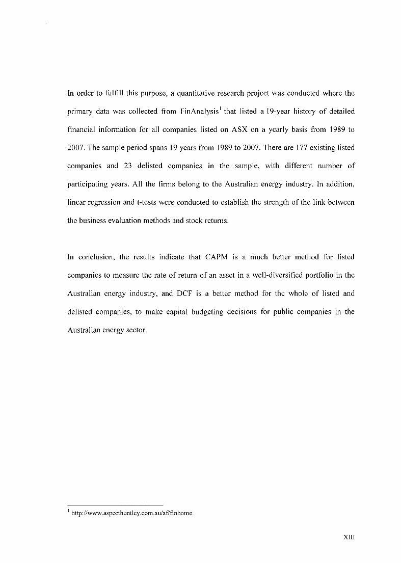
Chapter four will explain the data collected. The sample period spans 19 years from 1989

to 2007. There are 177 existing listed companies and 23 delisted companies in the sample

with different number of participating years of them. All the firms belong to the

Australian energy industry. Chapter five will examine the data analysis. The linear

regression methods and t-test were adopted to assess whether there are the strength of the

link between the business evaluation methods and share price.

Chapter six will critique seven business evaluation methods’ efficiency in Australian

energy sector. The chapter provides an overview of seven business valuation methods,

and provides the methodological processes and the empirical results. Chapter seven

outlines the limitations of this thesis and includes data collection problems, data

7

adjustment problems and transactions problems for the guideline companies as well as

further research study is advised. Chapter eight provides a summary and conclusion to the

seven valuation methods and discusses implications arising from the results.

8

CHAPTER TWO

THESIS OBJECTIVES AND CONTENTS

9

2.1 Thesis objectives

There are four main objectives of this thesis:

1) To present a review of the literature that explains and frames the business valuation

methods in the Australian energy sector.

2) To indicate data collection and data analysis of seven commonly used business

evaluation methods (CAPM, WACC, EVA, P/E ratio, DCF, MetaCapitalism and

Merger and Acquisition) in the whole market, listed market and delisted market.

3) To investigate how regression analysis has been conducted to develop an equation (a

linear regression line) for predicting a value of the dependent variables given a value

of the independent variable.

4) To perform a critical, thorough and detailed evaluation of business evaluation methods

during the period from 1989 to 2007 and to determine whether a correlation exists

between the business evaluation methods and the share price.

2.2 Organisation of contents

CHPTER 1-Introduction

The first chapter describes the basic introduction about this thesis, and establishes the

validity of the research by showing the previous research in the field contents.

CHPTER 2- Thesis Objectives

This chapter explores the main objectives of thesis.

10

CHAPTER 3 – Literature Review

The purpose of this chapter is to present a review of the literature which explains and

frames the business valuation methods in the energy companies in Australia.

CHAPTER 4 – Data Collection

This chapter describes data collection for seven commonly used business evaluation

methods.

CHAPTER 5 – Data Analysis

This chapter explores data analysis for seven commonly used business evaluation

methods.

CHPTER 6 – Critique and Discussion

Chapter six will discuss and critique seven business evaluation methods’ efficiency in the

Australian energy sector.

CHPTER 7 –Limitation and future research

This chapter examines three main limitations in this thesis and discusses the future study

contents.

CHPTER 8 – Conclusion

The conclusion will give the results of the research and the implications of the research.

11

CHAPTER THREE

LITERATURE REVIEW

12

3.1 Introduction:

The purpose of this chapter is to present a review of the literature which explains and

frames the business valuation methods in the energy companies in Australia. The aim of

any literature review is to provide a theoretical background and context for the study and

typically consistent of an interrelated set of statements, which can be used to explain or

understand the importance of the business valuation methods in the energy company.

This chapter is divided into three sections.

The first section identifies the most commonly used valuation methods that come from

221 articles are academic and related to the energy companies in Australia. The seven

commonly used business valuation methods were selected, they include CAPM (Capital

Asset Pricing Model), WACC (Weighted Average Cost of Capital), EVA (Economic

Valued Added), DCF (Discounted Cash Flow), P/E ratio Method, Guideline Merged and

Acquired Company Method and MetaCapitalism.

In the second section, previous research efforts into business valuation have been chosen

to analyze the four aspects for the seven business valuation methods. The first aspect

explores the overview of each method, including its history, first publication date, authors

and the causes for those methods. The second aspect describes each method. The third

aspect explains the methodology, including the analysis of the principles of methods,

rules, and postulates employed by a discipline. The fourth part gives the limitations of

each methods based on the literature review.

13

The last section examines the comparison of studies from previous literature. The

literature research explores the differences between the net present values (NPVs) of

North Sea oil projects obtained using the weighted average cost of capital and a modern

asset pricing (MAP) method which involves the separate discounting of project cash flow

components. The results obtained utilising the MAP method are very sensitive to the

choice of parameter values for the stochastic process used to model oil prices. Therefore,

more work should be done on the oil price model and the use of risk-free discounting of

costs before the MAP method can be adopted as the only valuation method.

3.2 Identifying most commonly used methods

Accountants and professional business valuers may use any number of business valuation

methods to determine the value of a business. The result of using these or other

approaches is in an attempt to determine a fair and reasonable price for a business.

Prospective buyers should calculate their own value and can use the advertised selling

price of a business as the basis to commence negotiations. Prospective purchasers must

scrutinise all those things that can affect the success, longevity and viability of a business.

This chapter lists some of the most commonly used evaluation methods which come from

221 articles consulted in this research.

14

3.1 Table: Most Commonly Used Evaluation Methods of Energy Industry

Total of Articles Found:

Method title Number of articles

mentioned / discussed the method

% frequently of method mentioned

Year of the first

publication Author

DCF 48 22% 1938 John Burr Williams

CAPM 41 18% 1963 William Sharpe EVA 26 12% 1982 Stern Steward WACC 36 16% 1963 Ezra Solomon Guideline merged and acquired company method

25 11% Late 1960s Unknown

P/E ratio method 31 14% 1960 Francis Nicholson MetaCapitalism 14 7 % 2000 Grady Means,

David Schneider Total 221 100%

3.3 CAPM (Capital Asset Pricing Model)

3.3.1 Overview

Hitchner (2006) describes that in 1952 economist Harry Markowitz, developed the

modern portfolio theory which presented the efficient frontier of optimal investment. In

1963, the research of William Sharpe has developed upon Markowitz’s portfolio theory,

in order to improve a means by which to measure this risk. William Sharpe who was a

student at the University of California was searching for a dissertation topic which

resulted in Markowitz suggesting that he explore the portfolio theory.

Sharpe studied the theory and modified it by connecting each portfolio with a single risk

factor. He put these risks into two categories, systematic risk and unsystematic risk.

Sharpe concluded that by diversifying one’s portfolio, one could reduce or eliminate

15

unsystematic risk. Therefore, the return of the portfolio would rest entirely on its

correlation to the market. This model has now come to be known as the capital asset

pricing model (Hitchner, 2006). The classic empirical studies, such as Fama and

MacBeth (1973), Gibbons (1982) and Stambaugh (1982) presented some evidence in

support of the formulation. The original formulation defined systematic risk as the

contribution to the variance of a well-diversified market portfolio (the beta).

3.3.2 Assumption

Patterson (1995, p.35) demonstrates the following assumption of the CAPM:

All models of security of price determination in capital markets are that all

investors hold well-diversified portfolios;

There are no transaction costs involved in trading securities;

All relevant information for the pricing of securities is freely and instantaneously

available to investors;

All assets are marketable and divisible;

These are no taxes that differentiate between securities or investors;

All investors have the same one-period investment horizon and have identical

views with respect to expected returns, variability, and the comovements of

returns for securities; and

All investors have the ability to borrow and lend unlimited amounts at a known

risk-free rate of R u f.

16

3.3.3 Methodology

The Capital Asset Pricing Model (CAPM) is used in finance to determine a theoretically

appropriate required rate of return of an asset, providing that the asset is to be added to an

already well-diversified portfolio and given that assets are a non-diversifiable risk.

According to Capital Asset Pricing Mode (2007), the CAPM formula takes into account

the asset’s sensitivity to non-diversifiable risk, often represented by the quantity beta (β)

in the financial industry, as well as the expected return of the market and the expected

return of a theoretical risk-free asset.

Cochrane (2001) claims that risk can be defined as the degree of uncertainty as to the

expectation of future returns and can be divided into three segments: maturity risk;

systematic risk; and unsystematic risk. In the capital market, the risk is divided risk into

two types:

1. Systematic Risk. The uncertainty of future returns due to the sensitivity of the return

on the subject investment to movements in the return for the investment market as a

whole (Cochrane 2001, p.200);

2. Unsystematic Risk. The uncertainty of future returns as a function of the characteristics

of the industry, company and type of investment interest. For example, circumstances can

impact unsystematic risk including operating in an industry subject to high obsolescence

(e.g., technology), management expertise, labor relations (Cochrane 2001, p.200).

17

The evidence shows that unsystematic risk can be freely eliminated by diversification,

and the reward for bearing risk depends only on the level of systematic risk. The level of

systematic risk in a particular asset relative to average is given by the beta of that asset.

According to Ross et al (2004, pp.374-375), the reward-to-risk ratio for Asset i is the

ratio of its risk premium, E(R m) - R f, to its beta, i m: [E(R m) - R f]/ i m. In a well-

functioning market, this ratio is the same for every asset. As a result, when expected

returns are plotted against asset betas, all assets plot on the same straight line, called the

security market line (SML). From the SML, the expected return on Asset i can be written:

E (R i) = R f + i m [E(R m) - R f].

3.1 Figure: the Security Market Line (SML)

18

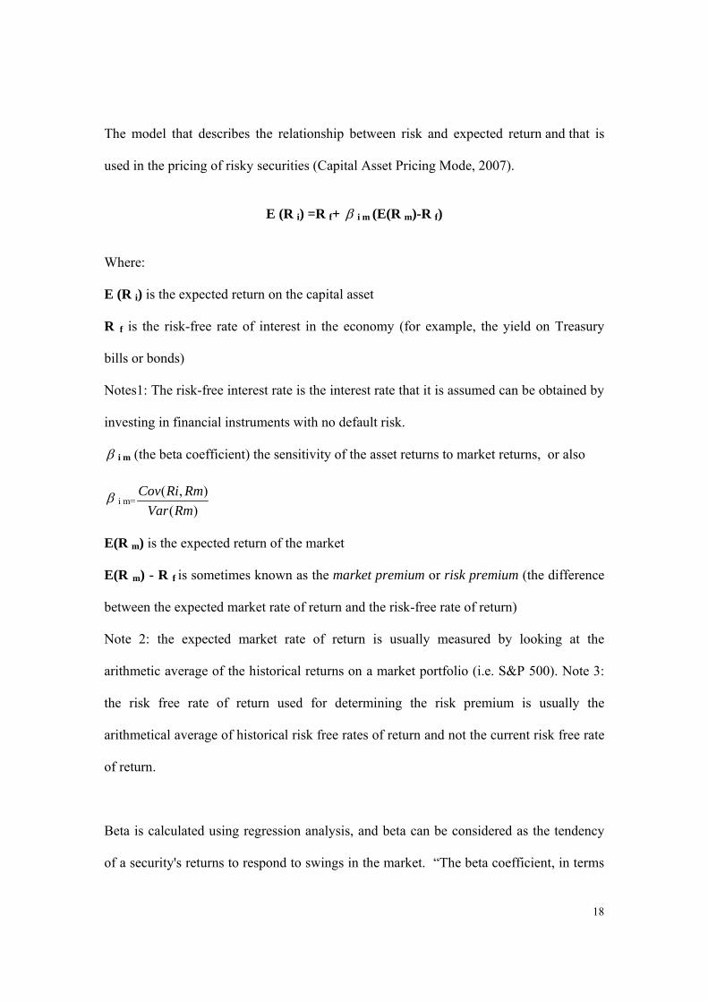
The model that describes the relationship between risk and expected return and that is

used in the pricing of risky securities (Capital Asset Pricing Mode, 2007).

E (R i) =R f+ i m (E(R m)-R f)

Where:

E (R i) is the expected return on the capital asset

R f is the risk-free rate of interest in the economy (for example, the yield on Treasury

bills or bonds)

Notes1: The risk-free interest rate is the interest rate that it is assumed can be obtained by

investing in financial instruments with no default risk.

i m (the beta coefficient) the sensitivity of the asset returns to market returns, or also

i m=( , )

( )

Cov Ri Rm

Var Rm

E(R m) is the expected return of the market

E(R m) - R f is sometimes known as the market premium or risk premium (the difference

between the expected market rate of return and the risk-free rate of return)

Note 2: the expected market rate of return is usually measured by looking at the

arithmetic average of the historical returns on a market portfolio (i.e. S&P 500). Note 3:

the risk free rate of return used for determining the risk premium is usually the

arithmetical average of historical risk free rates of return and not the current risk free rate

of return.

Beta is calculated using regression analysis, and beta can be considered as the tendency

of a security's returns to respond to swings in the market. “The beta coefficient, in terms

19

of finance and investing, describes how the expected return of a stock or portfolio is

correlated to the return of the financial market as a whole” (Gujarati 1992, p. 177).

According to research by Gujarati (2003, pp. 200-201), a beta of 0 means that its

security’s price is not at all correlated with the market. A beta of 1 indicates that the

security’s price will move with the market. A beta of less than 1 means that the security

will be less volatile than the market. A beta of greater than 1 indicates that the security’s

price will be more volatile than the market. For example, if a stock’s beta is 1.2, it is

theoretically 20% more volatile than the market. A negative beta shows that the asset

price inversely follows the market and its security’s price generally decreases in value if

the market goes up.

Research by Capital Asset Pricing Mode (2008) has shown that beta explores the

volatility of the security, relative to the asset class. The equation means that investors

require higher levels of expected returns to compensate them for higher expected risk.

This evidence proves that the formula can be considered as predicting a security’s

behaviour as a function of beta: CAPM is likely that if you know a security’s beta then

you know the value of E (R i) that investors expect it to have.

According to Francis & Grout (2000), the general idea behind CAPM is that investors

need to be compensated in two ways: time value of money and risk. The time value of

money is represented by the risk-free (rf) rate in the formula and compensates the

investors for placing money in any investment over a period of time. The other half of the

formula represents risk and calculates the amount of compensation the investor needs for

20

taking on additional risk. This is calculated by taking a risk measure (beta) that compares

the returns of the asset to the market over a period of time and to the market premium

(Rm-rf).

Francis & Grout (2000) claim that the expected return of a security or a portfolio equals

the rate on a risk-free security plus a risk premium. If this expected return does not meet

or beat the required return, then the investment should not be undertaken. The security

market line plots the results of the CAPM for all different risks (betas).

3.3.4 Limitation

Lvkovic (2007) gives some following limitations to CAPM:

The model assumes that asset returns are normally distributed random variables. It

is however frequently observed that returns in equity and other markets are not

normally distributed. As a result, large swings occur in the market more

frequently than the normal distribution assumption would expect ;

The model assumes that the variance of returns is an adequate measurement of

risk. This might be justified under the assumption of normally distributed returns,

but for general return distributions other risk measures will likely reflect

investors preference more adequately;

21

Model does not appear to adequately explain the variation in stock returns.

Empirical studies show that low beta stocks may offer higher returns than the

model would predict;

The model assumes that given a certain expected return investors will prefer

lower risk (lower variance) to higher risk and conversely given a certain level of

risk will prefer higher returns to lower ones. It does not allow for investors who

will accept lower returns for higher risk;

The model assumes that all investors have access to the same information and

agree about the risk and expected return of all assets;

The model assumes that there are no taxes or transaction costs, although this

assumption may be relaxed with more complicated versions of the model;

The market portfolio consists of all assets in all markets, where each asset is

weighted by its market capitalization. This assumes no preference between

markets and assets for individual investors, and that investors choose assets solely

as a function of their risk-return profile; and

The market portfolio should in theory include all types of assets that are held by

anyone as an investment. In practice, such a market portfolio is unobservable and

people usually substitute a stock index as a proxy for the true market portfolio.

22

3.4 WACC (Weighted Average Cost of Capital)

3.4.1 Overview

Solomon (1963) states that business education has undergone fundamental

transformation during 1950s in the United States. This transformation has been

characterised by intensive application to managerial problems of the underlying

disciplines - the social sciences, modern mathematics and statistics, a greater emphasis on

analysis rather than description in the teaching process and the development of

fundamental research on the business process.

In order to speed the diffusion of these social sciences, Ezra Solomon has demonstrated

that the minimum acceptance level of return for an incremental investment is equal to the

rate of discount which equates the flow of future payments to owners and creditors with

the current value of the firm in 1963. Within the framework of Solomon’s restrictive

assumptions, this true cost of capital is identical to the weighted average cost of capital

(Raymond & William 1973, p.123). Thus, incremental investments yielding at least the

weighted average cost of capital provide a net return on the equity capital, which is at

least equal to the rate of return required by the owners of the firm.

3.4.2 Assumption

According to Emhjellen & Alaouze (2002), the general assumptions required before the

weighted average cost of capital can be estimated:

23

Business risk - the risk to the firm of being unable to cover operating costs-is

assumed to be unchanged. This means that the acceptance of a given project does

not affect the firm’s ability to meet operating costs;

Financial risk - the risk to the firm of being unable to cover required financial

obligations-is assumed to be unchanged. This means that the projects are financed

in such a way that the firm’s ability to meet financing costs is unchanged;

After-tax costs are considered relevant-the cost of capital is measured on an after-

tax basis;

There are no costs of financial distress and liquidation (if a firm is liquidated,

shareholders will receive the same as the market value of their share prior to

liquidation); and

There are perfect capital markets, with perfect information available to all

economic agents and no transaction costs.

3.4.3 Methodology

Research by Hitchner (2006), the weighted average cost of capital (WACC) is the

average of the cost of equity and debt, weighted by the proportions of equity and debt

which an efficiently financed company can be expected to use to fund its activities.

Hence to determine the WACC, it is necessary to determine the cost of debt and the cost

24

of equity and the proportions of debt and equity that would be employed by an efficiently

financed company.

Evidence from Pratt (1998, pp.45-46) shows that WACC is especially correct for project

selection in capital budgeting. The percentage of debt and equity that could be available

to finance different kinds of projects could be different and the cost of capital should be

based on the specific investment. This evidence has shown that the weight for each

component of the capital structure should be calculated to determine the entire capital

structure and the relative weightings of debt and equity or other capital components are

based on the market values of each component rather than on the book values.

According to Weighted Average Cost of Capital (2002, p.10), in earlier reviews and

determinations by Australian Regulators, the cost of capital was commonly expressed as

a pre-tax real WACC. However, the regulators generally commented that the cost of

capital would be reviewed in light of future developments.

Recently, the Australian Competition and Consumer Commission (ACCC) and

Queensland Competition Authority (QCA) have released determinations where the

WACC has been formulated based on a nominal post-tax approach. The Essential

Services Commission (ESC) has adopted a real post-tax approach, while the Office of

Gas Access Regulation (Ofgar) still expresses the WACC in terms of pre-tax real

(Weighted Average Cost of Capital 2002, p.16).

25

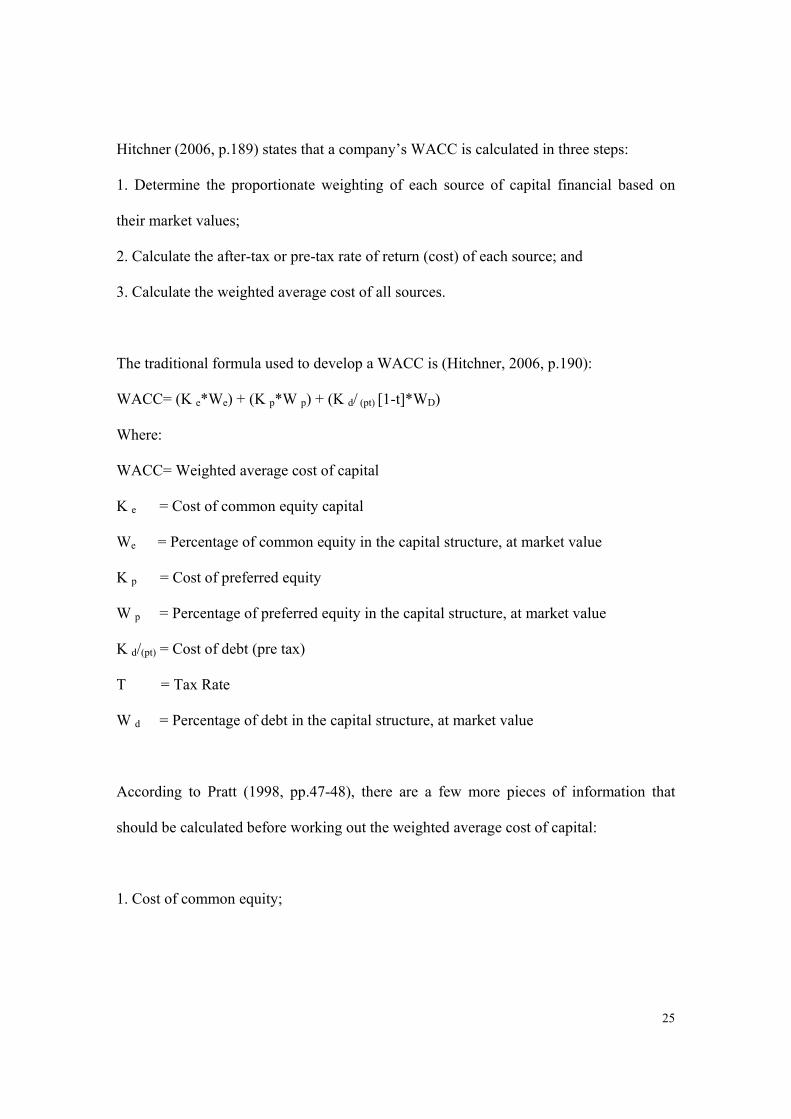
Hitchner (2006, p.189) states that a company’s WACC is calculated in three steps:

1. Determine the proportionate weighting of each source of capital financial based on

their market values;

2. Calculate the after-tax or pre-tax rate of return (cost) of each source; and

3. Calculate the weighted average cost of all sources.

The traditional formula used to develop a WACC is (Hitchner, 2006, p.190):

WACC= (K e*We) + (K p*W p) + (K d/ (pt) [1-t]*WD)

Where:

WACC= Weighted average cost of capital

K e = Cost of common equity capital

We = Percentage of common equity in the capital structure, at market value

K p = Cost of preferred equity

W p = Percentage of preferred equity in the capital structure, at market value

K d/(pt) = Cost of debt (pre tax)

T = Tax Rate

W d = Percentage of debt in the capital structure, at market value

According to Pratt (1998, pp.47-48), there are a few more pieces of information that

should be calculated before working out the weighted average cost of capital:

1. Cost of common equity;

26

Regulatory decisions in Australia have generally determined that the cost of equity is

calculated using CAPM (Weighted Average Cost of Capital 2002, p.6).

2. Cost of preferred equity;

“A measure of equity only takes into account the preferred stockholders, and disregards

the common stockholders. It is equal to shareholders’ equity minus common equity”

(Pratt 1998, p. 47).

3. Cost of debt (before tax effect).

Regulatory decisions in Australia have generally determined the cost of debt as a margin

over the risk free rate (Weighted Average Cost of Capital 2002, p.13).

Evidence by Benninga (2000, p. 39), the cost of debt can be calculated as:

Total debt = long term debt + short tern dent and current portion of long term debt

Cost of debt = interest expense / total debt

4. Tax rate.

Presently, the value for tax is a prominent issue. Regulatory decisions have begun to

adopt effective tax rates rather than use the statutory rate (Weighted Average Cost of

Capital 2002, p.8).

3.4.4 Limitations

Lund (2000) lists the following two limitations to WACC:

27

Its main limitation is that it is only applicable to assets that have the same

systematic risks and incremental debt ratio as the traded equity used to estimate its

magnitude. In general, for assets that do not meet this criterion, it is still necessary

to estimate a project-specific level of K j;

The premise of weighted average cost of capital is that an investor would pay no

more to purchase the asset than would be paid to reproduce the asset. While this

approach is suitable for some assets, particularly those which are not directly

generating income, choosing this approach as cost is not always a reliable guide to

value, for example, the vast amounts of money spent on pharmaceutical research

projects which come to nothing.

3.5 DCF (Discounted Cash Flow)

3.5.1 Overview

Discounted Cash Flow (DCF) calculations have been used in some forms since money

was first lent at interest in ancient times. As a method of asset valuation it has often been

opposed to accounting book value, which is based on the amount paid for the asset

(Discounted Cash Flow - DCF, 2008). Discounted Cash Flow was first formally

published in 1938 in a text by John Burr Williams. This was after the market crash of

1929 and before auditing and public accounting was mandated by the SEC. Due to the

economic crash, investors were wary of relying on the reporting earnings, or in fact any

measures of value apart from cash (Discounted Cash Flow - DCF, 2008). Therefore,

discounted cash flow analysis gained popularity as a valuation method for stocks.

28

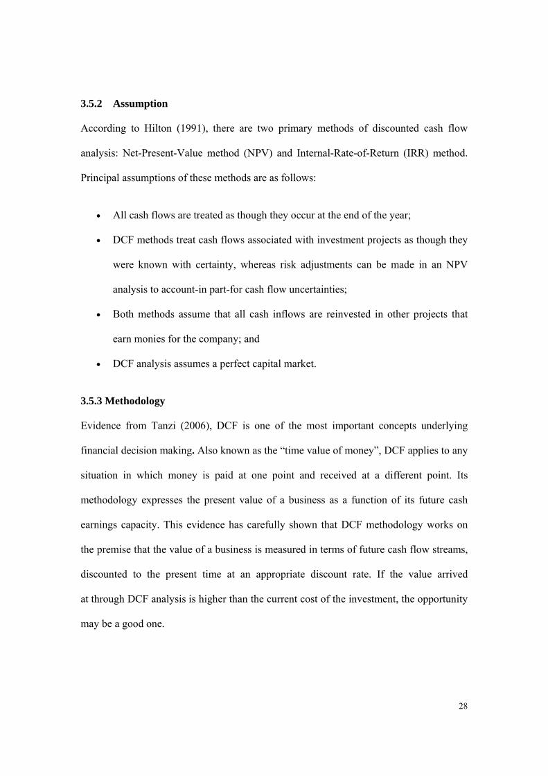
3.5.2 Assumption

According to Hilton (1991), there are two primary methods of discounted cash flow

analysis: Net-Present-Value method (NPV) and Internal-Rate-of-Return (IRR) method.

Principal assumptions of these methods are as follows:

All cash flows are treated as though they occur at the end of the year;

DCF methods treat cash flows associated with investment projects as though they

were known with certainty, whereas risk adjustments can be made in an NPV

analysis to account-in part-for cash flow uncertainties;

Both methods assume that all cash inflows are reinvested in other projects that

earn monies for the company; and

DCF analysis assumes a perfect capital market.

3.5.3 Methodology

Evidence from Tanzi (2006), DCF is one of the most important concepts underlying

financial decision making. Also known as the “time value of money”, DCF applies to any

situation in which money is paid at one point and received at a different point. Its

methodology expresses the present value of a business as a function of its future cash

earnings capacity. This evidence has carefully shown that DCF methodology works on

the premise that the value of a business is measured in terms of future cash flow streams,

discounted to the present time at an appropriate discount rate. If the value arrived

at through DCF analysis is higher than the current cost of the investment, the opportunity

may be a good one.

29

The discounted cash flow formula is derived from the future value formula for

calculating the time value of money and compounding returns (Kruschwitz & Loffler,

2005).

FV=PV*(1+i) n

The simplified version of the discounted cash flow equation (for one cash flow in one

future period) is expressed as:

DPV= FV

(1+i)n = FV (1-d) n

Where,

DPV is the discounted present value of the future cash flow (FV), or FV adjusted

for the opportunity cost of future receipts and risk of loss;

FV is the nominal value of a cash flow amount in a future period;

d is the discount rate, which is the opportunity cost plus risk factor (or the time

value of money: “I” in the future-value equation);

n is the number of discounting periods used (the period in which the future cash

flow occurs). I.e. if the receipts occur at the end of year 1, n will be equal to 1; at

the end of year 2, 2-likewise, if the cash flow happens instantly, n becomes 0,

rendering the expression an identity (DPV=FV).

Kruschwitz & Loffler (2005) explore that NPV is the difference between the present

value of cash inflows and the present value of cash outflows. NPV is used in capital

30

budgeting to analyse the profitability of an investment or project. This is also called the

net present value method.

Where value is the investment’s net present value, C0 is the certain after-tax cash flow at

time 0, E (Ct) is the expected after-tax cash flow at time t, T is the investment’s life, and r

is the risk adjusted discount rate.

Benninga (2000) outlines four different DCF methods depending on the financing

schedule of the company today. Due to different underlying financing assumptions, the

value of the project or company do not need to arrive at the same. The following is the

four DCF methods:

Equity-Approach

o Flows to equity approach (FTE)

Entity-Approach:

o Adjusted present value approach (APV)

o Weighted average cost of capital approach (WACC)

o Total cash flow approach (TCF)

This thesis will focus on the free cash flow to equity approach to determine the “fair

value” of companies. The first step for using discounted cash flow (DCF) analysis is to

determine how far out into the future we should project cash flows.

31

3.2 Table: good guideline to use when determining a company’s forecast period

(Benninga 2000, p. 64):

Company Competitive Position Forecast Period

Slow-growing company; operates in highly competitive, low margin industry

1 years

Solid company; operates with advantage such as strong marketing channels, recognizable brand name, or regulatory advantage

5 years

Outstanding growth company; operates with very high barriers to entry, dominant market position or prospects

10 years

The second step is to define the free cash flow. The easiest way to define the free cash

flow is as following (Benninga 2000, p. 65):

Defining the Free Cash Flow

Profit after taxes

This is the basic measure of the profitability of the business, but it is an accounting measure that includes financing flows, as well as noncash expenses such as depreciation. Profit after taxes does not account for either changes in the firm’s working capital or purchase of new fixed assets, both of which can be important cash drains on the firm.

+Depreciation+ after tax interest payments

Depreciation should be added back to the profit after tax. FCF is an attempt to measure the cash produced by the business activity of the firm. We should add back the after tax cost of interest on debt, and subtract out the after tax interest payments on cash and marketable securities.

-Increase in current assets

Since the firm’s sales increase, more investment should be put in inventories, accounts receivable, etc. This increase in current assets is not an expense for tax purpose.

+Increase in current liabilities

An increase in the sales often causes in financing related to sales. This increases in current liabilities.

-Increase in fixed assets at cost

32

An increase in fixed assets is a use of cash, which reduces the firm’s free cash flow.

The enterprise value of the firm is defined to be the value of the firm’s debt, convertible

securities and equity. “In financial theory, the enterprise value is the present value of the

firm’s future anticipated cash flows. Accordingly, the enterprise value of the firm is the

discounted value of the firm’s projected FCF plus its terminal value” (Benninga 2000, p.

68).

Enterprise value= FCF1/ (1+WACC) 1+FCF2/ (1+WACC) 2+……………………...

FCF5/ (1+WACC) 5+Year 5 terminal value/ (1+WACC)

There are several ways to estimate a terminal value of cash flows, but one well-known

method is to value the company as a perpetuity using the Gordon Growth Model. The

model uses this formula (Benninga 2000, p. 70):

Terminal Value = Final Projected Year Cash Flow X (1+Long-Term Cash Flow Growth Rate)

(WACC – Long-Term Cash Flow Growth Rate)

Calculating the Fair Value of Equity (Benninga 2000, p. 72):

Fair Value of Company Equity = Enterprise Value – Debt

We can judge the value of the company shares when having finished the DCF valuation.

If the shares are trading at a lower value than this, they could represent a buying

opportunity for investors. If they are trading higher than the per share fair value,

33

shareholders may want to consider selling the company shares. The formula has shown as

the following (Benninga 2000, p. 73):

Share Price = Fair Value of Company Equity / Shares Outstanding

3.5.3 Limitation

Research by Baur, Habib & Volkart (1998), due to the difficulty of forecasting into the

future, some constant rate of growth in cash flow must be assumed beyond some future

year. In general, valuation is extremely sensitive to this growth rate, which is necessarily

assumed to go on forever. This research explores that the choice of the growth rate can be

made to serve some party’s agenda and satisfy their self interests. Therefore, this

naturally damages the credibility of DCF valuations and causes the severe consequences

for the public interest.

“A limitation of the NPV is that it is not related to the size of the project. If one project

has a slightly lower NPV than another, but the capital outlays required are much lower,

then the second project will probably be the preferred one” (Baur, Habib & Volkart 1998,

p. 124). In addition, DCF is merely a mechanical valuation tool, which makes it subject

to the axiom “garbage in, garbage out”. Small changes in inputs can result in large

changes in the value of a company (Baur, Habib & Volkart, 1998).The evidence has

shown that DCF models are powerful but they do have shortcomings. NPV has the larger

problem in using DCF to evaluate the business performance because it can affect the size

of the project. The DCF model is only a mathematical formula that people can utilize in

order to reduce mistakes to achieve increased profits.

34

3.6 P/E ratio

3.6.1 Overview

The P/E ratio has been known for almost fifty years and is widely used to describe a

company’s business activity. Evidence by Board (2005, p.5) shows that a large amount of

academic work has demonstrated the effect and attempted to decide whether it is real or a

proxy for other factors. The first work demonstrating P/E effect was the research

published in 1960 by Nicholson. He collected 100 mainly industrial stocks over five-year

periods from 1939 to 1959. The portfolio of lowest P/E quintile stock, rebalanced every

five years, would have delivered an investor 14.7 times his original investment at the end

of the twenty years, as compared to 4.7 times for the highest P/E quintile.

3.6.2 Assumption

Albrecht (1990, pp.2-3) states the assumption for P/E ratio, it is not significantly different

from the average firm in the industry in terms of expected earnings growth rate and risk

or that the differences off-set each other. And it should be recognized that both the

growth rate of earnings and risk would be controlled by market forces which are common

to all firms in the industry. Certainly, assuming average performance is a reasonable

assumption.

3.6.3 Methodology

According to Price-Earnings-Ratio (2007), the P/E ratio (price to earnings ratio) of a

stock is a measure of the price paid for a share related to the annual income or profit

earned by the firm per share. When it comes to valuing stocks, the price/earnings ratio is

one of the oldest and most frequently used metrics. It can be seen that a high P/E suggests

35

that investors are expecting higher earnings growth in the future compared to companies

with a lower P/E. However, the P/E ratio doesn’t tell us the whole story by itself. It’s

usually more useful to compare the P/E ratios of one company to other companies in the

same industry, to the market in general or against the company’s own historical P/E.

P/E is short for the ratio of a company’s share price to its per-share-earnings. Basically,

the P/E ratio formula is set as the following (Price-Earnings-Ratio, 2007):

P/E ratio = Price per Share

Annual Earning per Share

The price per share is the market price of a single share of the stock;

The earnings per share are the net income of the company for the most recent 12

month period, divided by number of shares outstanding. The earnings per share

(EPS) used can also be the “diluted EPS”, or the “comprehensive EPS”.

Its formula is: EPS=Net Income / Average Outstanding Shares

According to research by Little (2004), in the EPS calculation, it is more accurate to use

a weighted average number of shares outstanding over the reporting term, because

the number of shares outstanding can change over time. However, data

sources sometimes simplify the calculation by using the number of shares outstanding at

the end of the period.

Ordinarily, the P/E is calculated using EPS from the last four quarters. This is also known

as the trailing P/E. However, occasionally the EPS figure comes from estimated earnings

expected over the next four quarters. This is known as the leading or projected P/E

36

(Durell, 2006).

Durell (2006) demonstrates that a stock’s P/E tells us how many investors are willing to

pay per dollar earnings. For this reason it’s also called the “multiple” of a stock. This

evidence has shown that a P/E ratio of 20 means that investors in the stock are willing to

pay $20 for every $1 of earnings that the company generates.

3.6.4 Limitation

Sayeed (2008) states the three aspects of P/E ratio limitation, as the following:

Accounting: There are too many methods to calculate the actual earnings per

share (EPS), such as Primary EPS, Diluted EPS, and Headline EPS etc. Moreover,

some investors can use the different way to calculate may get confused between

the different types of EPS and thus reach a wrong P/E estimate;

Inflation: during the periods of high inflation, inventory and depreciation costs

may be understated because the replacement costs of goods and equipment rise

with the general level of prices. Thus, P/E ratios tend to be lower during times of

high inflation because the market sees earnings as artificially distorted upwards;

Besides earnings, there are other factors that affect the value of a stock. For

example:

o Brand - The name of a product or company has value. Brands such as

Coca-Cola are worth billions;

o Human Capital - A company’s employees and their expertise are should

add value to the company;

37

o Expectations - The stock market is forward looking. People buy a stock

because of high expectations for strong profits, not because of past

achievements; and

o Barriers To Entry - For a company to be successful in the long run, it must

have strategies to keep competitors from entering the industry.

All these factors will affect a company’s earnings growth rate. Because the P/E ratio uses

past earnings (trailing twelve months), it gives a less accurate reflection of these growth

potentials.

3.7 EVA (Economic Value Added)

3.7.1 Overview

“EVA (Economic Value Added) was developed by a New York Consulting firm, Stern

Steward & Co in 1982 to promote value-maximizing behaviour in corporate managers”

(Worthington & West 2001, p.6). It is a single, value-based measure that was intended to

evaluate business strategies, capital projects and to maximize long-term shareholders

wealth (Worthington & West 2001, p.7). This evidence states that EVA can be measured

by comparing profits with the cost of capital used to produce them and it can help

managers decide to withdraw value-destructive activities and invest in projects that are

critical to shareholder’s wealth. Therefore, this will lead to an increase in the market

value of the company.

Sharma (2004) describes that Cola-Cola is one of many companies that adopted EVA for

measuring its performance. Coca-Cola CEO Roberto Goizueta accredited EVA for

turning Coca-Cola into the number one Market Value Added Company. Coca-Cola’s

38

stock price increased from $3 to over $60 when it first adopted EVA in the early 1980s.

In 1995, Coca-Cola’s investor received $8.63 wealth for every dollar they invested.

3.7.2 Methodology

According to Banerjee (2000), Economic Value Added (EVA) may be defined as the net

operating profits after tax minus an appropriate charge for the opportunity cost of all

capital invested in an enterprise. Thus

EVA = Net Operating Profit after tax – Weighted Average Cost of Capital

EVA can be rewritten as:

EVA = (ROI – WACC)*CAPITAL EMPLOYED

ROI=NOPAT

K , called the return on invested capital

Capita Employed: represents the total cash investment that shareholders and debt

holders have made in a company. There are two different but completely

equivalent methods for calculating invested capital.

The operating approach is calculated as:

Invested capital = Operating Net Working Capital + Net PP&E + Capitalized

Operating Leases + Other Operating Assets + Operating Intangibles – Other

Operating Liabilities – Cumulative Adjustment for Amortization of R&D.

The financing approach is calculated as:

39

Invested Capital= Total Debt and Leases + Total Equity and Equity Equivalents-

Non-Operating Cash and Investments

“EVA captures the fact that equity should earn at least the return that is commensurate to

the risk that the investor takes” (Mark1996, p.45). This evidence has shown that equity

capital has to earn at least same return as similarly risky investments at equity markets. If

that is not the case, then there is no real profit made and actually the company operates at

a loss from the viewpoint of shareholders. On the other hand, if EVA is zero, this should

be treated as a sufficient achievement because the shareholders have earned a return that

compensates the risk.

Sharma (2004) also claims several advantages for EVA:

1. EVA eliminates economic distortions of GAAP to focus decisions on real economic

results;

2. EVA provides for better assessment of decisions that affect balance sheet and income

statement or tradeoffs between each through the use of the capital charge against NOPAT;

3. EVA decouples bonus plans from budgetary targets;

4. EVA covers all aspects of the business cycle; and

5. EVA aligns and speeds decision making, and enhances communication and teamwork.

3.7.3 Limitation

40

EVA also has its critics. The biggest limitation is that the only major publicly-available

sample evidence on the evidence of EVA adoption on firm performance is an in-house

study conducted by Stern Stewart and except that there are only a number of single-firm

or industry field studies.

Keys, Azamhuzjaev & Mackey (2001) cite the following limitations to EVA:

EVA does not control for size differences across plants or divisions;

EVA is based on financial accounting methods that can be manipulated by

managers;

EVA may focus on immediate results which diminishes innovation; and

EVA provides information that is obvious but offers no solutions in much the

same way as historical financial statement do.

Also, Huang (2007) identifies the following two limitations of EVA:

Given the emphasis of EVA on improving business-unit performance, it does not

encourage collaborative relationship between business unit managers;

EVA although a better measure than EPS, PAT and RONW is still not a perfect

measure.

3.8 Guideline Merged and Acquired Company Method

3.8.1 Overview

According to Koller, Goedhart & Wessels (2005, p. 427), Mergers and acquisitions (M &

A) have long been features of the corporate landscape. They first became notorious in the

late 1800s in the United States with the activity of the “robber barons”, followed by the

41

consolidations of J.P. Morgan and others in the early 1900s. Since then, there have been

several waves of M& A activity in the United States-during the booming economy of the

late1960s, through to the controversial wave of restructuring in the in the mid-1980s and

most recently with the megadeals signed during the late 1990s.

3.8.2 Assumption

Hitcher (2006, pp. 270-273) outlines the several assumptions as the following:

The company’s expected growth in sales or earnings is most important

assumption in a guideline price multiple. And the short-term and perpetual growth

rates are listed as assumptions;

Other important assumptions such as expected risk and margins are not explicitly

given. The implicit prices of publicly traded companies and transactions are some

assumption about growth. Commonly, the higher the expected growth, the higher

the value, all the things are equal; and

In addition, it is difficult to get the detailed financial statements of the acquired

company, so it is impossible to make certain adjustments to the data underlying

the pricing multiples.

3.8.3 Methodology

According to Wise (2003), Guideline Merger and Acquisition method involves the

valuation ratios derived from transactional pricing information that is related to the

appropriate underlying financial data of guideline companies, and then applied to the

corresponding data of the subject company to arrive at an indication of value. The

42

analysis involves the comparison of the respective qualitative and quantitative factors

relating to the company being valued to those of the guideline companies.

Evidence by Hitcher (2006, pp.270-271), at its simplest, the method requires only

multiplication and perhaps some subtraction, depending on the multiple selected. The

basic format is (Hitcher, 2006):

Value subject = [( Price

Parameter ) comps*Parameter subject] – Debt Subject

Parameter might be sales, net incomes, book value.

The Price / Parameter multiple is the appropriate pricing multiple based on that parameter

(e.g., price/ net income, price/ book value) and taken from the guideline companies. In

some cases (invested capital multiples) the debt of the subject company may have to be

subtracted.

Basic Financial Indicators (Hitcher, 2006, pp. 288-292):

Some financial measures that should be included in an analysis for both guideline and

subject companies include:

Size Measures. These include the magnitude of sales, profits, total assets, market

capitalization, and total invested capital;

Historical Growth Rates. Consider growth in sales, profits, assets or equity;

Measures of Profitability and Cash Flow. Consider the four most common

measures:

43

1. Earning before interest, taxes, depreciation and amortization (EBITDA)

2. Earnings before interest and taxes ( EBIT)

3. Net income

4. Cash flow

Profit Margins. The current level of profits is probably less important than the

ratio of profits relative to some base item-usually sales, assets, or equity;

Capital Structure. It is essential to use some measures derived from the current

capital structure; and

Other Measures. These will be a function of what is important in the industry in

which the subject company operates.

Displaying the Information (Hitcher, 2006, pp. 292-293):

The key items have been chosen, the next stage is to put the information into a usable

format. These data should be displayed in order to make comparisons easy. Further, so

that comparisons are meaningful, the concepts must be consistent across companies. The

financial information for the subject company should be shown in a consistent format.

Financial statement measures (Hitcher, 2006):

The second part of the pricing multiple is the denominator, the financial statement

parameter that scales the value of the company. The four general groupings of valuation

ratios include those based on:

1. Revenues;

2. Profitability or cash flows;

44

3. Book values; and

4. Some other measure.

Matching price to parameter (Hitcher, 2006, p.303):

Conventionally, price has been matched to the appropriate parameter based on which

providers of capital in the numerator will be paid with the monies given in the

denominator.

Dispersion of pricing multiples (Hitcher, 2006, pp.305-306):

The coefficient of variation is a useful statistic for analyzing multiples. It measures the

dispersion of the data relation to its average value. The higher the coefficient of

variation, the larger the range of pricing multiples.

Applying the valuation multiples (Hitcher, 2006, pp. 305-310):

The final step is to apply the valuation multiples to the subject company. The companies

that remain in the guideline company set are usually ones that should be reasonably

comparable to the subject.

3.8.4 Limitation

Palepu, Healy & Bernard (2004) cite the three limitations of Guideline Merger and

Acquisition method as the following:

45

No good guideline companies exist. This is the bigger reason the approach is not

used in a valuation. Possibly, it is difficulty to find guideline companies that are

sufficiently similar to the subject;

Due to hart to obtain the detailed financial data, so some assumptions about the

adjustments and growth are incorrect; and

It is not as flexible or adaptable as other approaches. The market approach is hard

to include unique operating characteristics of the firm in the value it produces.

3.9 MetaCapitalism

3.9.1 Overview

MetaCapitalism is e-business revolution and the design of 21st-century companies and

markets (Means & Schneider, 2000); it is also the new corporate strategy that requires

companies to follow if they are going to succeed in the competitive business world

(Means & Schneider, 2000). MetaCapitalism advocates a radical or extreme outsourcing

and downsizing of human capital, de-capitalization of all non-core capital assets and the

diminished role of the State in the global free market economy (Mickhail and Ostrovsky,

2007). These transformations requires the traditional companies to shift to internet-

leveraged styles of brand-owning, customer-focused companies and the company should

focus on the business-to-business (B2B) e-business revolution, in order to archive the

economy growth and value creation (Mickhail and Ostrovsky, 2007).

3.9.2 Assumption

3.9.2.1 Downsizing

46

Under the MetaCapitalism model, the downsizing achieved by recapitalizing non-core

base which includes both physical and human capital. “Clearly, spinning off

manufacturing and related operating processes, generally to an outsourced network, frees

up enormous amounts of capital that can be focused on brand development, customers

ownership, supply network management, and other industry leadership processes”

(Means & Schneider, 2000, p. 7).

3.9.2.2 Recapitalization

The purpose of recapitalization or outsourcing is to reduce the firm’s non-core physical

assets. “Accompanying the dramatic effort to lower the base of physical capital and

outsource is an equally dramatic effort to lower working capital. As brand owners

outsource parts manufacture, physical product systems, and large chunks of final

assembly for their proprietary, designs and branded products, they keep little if any

manufacturing inventory in-house” (Means & Schneider, 2000, p. 6).

Outsourcing became part of the business lexicon during the 1980s and refers to the

delegation of non-core operations from internal production to an external entity

specializing in the management of that operation. Outsourcing is utilizing experts from

outside the entity to perform specific tasks that the entity once performed itself (Mickhail

and Ostrovsky, 2007).

3.9.2.3 Value Added Communities

47

Effective VAC’s main assumption is that all firms will act efficiency and cooperatively

for the mutual benefit. The model does not take into account that there are inherently

conflicting commercial interests between these firms (Mickhail and Ostrovsky, 2005).

VACs assumption ignored the inherent characteristic for the companies and social

environments that caused possible impacts to the companies.

3.9.3 Methodology

The MetaCapitalism equation is used as a means of reducing the strategy to a measurable

index. The core tenets of MetaCapitalism are decapitalisation, outsourcing and

downsizing and these can be measured by PP&E, NWC and NOE (Means & Schneider,

2000). Measure a firm’s level of MetaCapitalisation by calculating its composite change

value over time, based on:

NMC + PP&E +NOE + R&D

TA

This equation, and in particular the corresponding ratios, were taken to indicate the level

of MetaCapitalisation because they precisely represent the main tenets of the strategy of

decapitalisation (ie: Net Working Capital or NWC), selling of physical assets (Plant

Property and Equipment or PPE), and reduction in the number of employees through

downsizing and outsourcing (Number of Employees or NOE).

The highest negative change in each index represents an aggressive application of the

strategy through to the highest positive change, which represents passive application or

no application at all. It was then possible to categories the firms into groups, in the order

48

of the largest negative change in value of their MetaCapitalisation downwards (Mickhail

and Ostrovsky, 2007).

A=L+OE(R-E)

Asset declines because of the de-capitalization of all non-core capital assets (Lower

PP&E, better use of Net Working Capital or NWC). Also, liability decrease (lower Long

Term Debt); and reduction in the number of employees through downsizing and

outsourcing lead to reduce of expenses (lower NoE, lower Transaction and Procurement

Cost). Therefore, the profit increases.

Due to a lack of available information, the analysis on the NOE has been excluded and

leaves six remaining indices to be tested. The original combined index was separated into

the following individual indices (Farrell, 2005).

NWC Change

PP & E Change

TA Change

NWC/TA Change

PP & E /TA Change

NWC +PP&E/TA Change

The formula is comprised of six parts which compare the change in the share price. The

formula indicates which indices are responsible for adverse effects. The period signifies

which MetaCapitalism indices change correlates to the share price change.

49

3.10 Comparison of studies from literature

3.10.1 Introduction

According to Emhjellen & Alaouze (2002, p. 1213), the purpose of this study is to

examine the difference between oil project NPVs obtained using the discounted cash

flow method and a modern asset pricing (MAP) method and to identify any implications

this might have for the project selection of energy companies. And the recommendation

should be provided to change from the weighted average cost of capital (WACC)

discounting method to the MAP discounting method.

Emhjellen & Alaouze (2002, p. 1214) highlights that the MAP approach should give

better NPV estimates than the WACC method, the reason is that the MAP method

discounts revenues and costs using discount rates that reflect the riskiness of each cash

flow component. The MAP approach uses a discount rate for revenue that incorporates

oil price volatility, a risk parameter, mean reversion of oil prices and time. However,

MAP discounting method is very sensitive to the choice of the value for the parameters of

the stochastic process used to model oil prices. Therefore, before the MAP method can be

adopted as the only valuation method, more work should be done on the oil price model

and the use of risk-free discounting of costs.

3.10.2 Valuation based on the WACC

Emhjellen & Alaouze (2002, pp. 1214-1215) explain the oil projects valuation based on

the WACC. The oil exploration projects are in the North Sea and are subject to the

Norwegian tax regime. Oil companies are invited to apply for interests in exploration

50

areas when these are made available by the Norwegian government. The oil projects

structure come from two to five companies participating in planning and development of

the project.

“The project NPV were calculated using the WACC as the discounted rate and the NPV

of the portfolio was found to be $US 1236.9 million. However, project 1 was found to

have a negative NPV, it was removed from the portfolio and the NPV of the portfolio

changed to $ US 1251.3 million” (Emhjellen & Alaouze 2002, pp. 1214-1215).

3.10.3 Valuation using a derivative asset methodology

Research by Emhjellen & Alaouze (2002, pp. 1215-1216), The PV of a barrel of oil (V0

(PT)) is given by Laughton and Jacoby (1993) as:

V0 (PT) =E0 (PT) exp (- (1-exp (- t))/ ) exp(-it), (3.0)

Where the risk discount factor is equal to RDF t= exp (- (1-exp (- t))/ ), the time

discount factor is equal to TDF t = exp(-it) ( with I being the real risk-free rate), E0(PT) is

the expected real oil price at time t as determined at time zero, is the risk adjustment

parameter of oil prices, is the volatility factor of oil prices and is the rate of mean

reversion of oil prices.

In the excel spreadsheet model used to calculate project values, the risk discount factor is

calculated as:

RDF t= exp (- (1-exp (- t))/ ), (3.1)

Risk-free discounting for time is performed utilising

RDF t= exp (-it)/k t (3.2)

51

In Eq. (3.2) i is the real risk-free rate and k t is the inflation factor, which is defined as k

t=kt-1 exp (k), which k o=1 and k the constant inflation rate.

Project NPV was calculated using the formula

NPV= R ct - C ct - T ct (3.3)

Where R ct is the sum of the PV s of the expected real revenue cash flows,

C ct is the sum of the PV s of the expected real cost cash flows and T ct is the

sum of the PV s of the expected real tax cash flows.

Evidence by Emhjellen & Alaouze (2002, pp. 1217-1218), a comparison of the project

NPVs obtained using the WACC discounting method with the project NPV obtained

using the MAP method shows that the most undervalued projects are projects N (_14

million dollars), G (_12 million dollars) and J (_8.4 million dollars). The most overvalued

are projects D (9.3 million dollars), B (8.3 million dollars), C (7.5 million dollars) and E

(6.1 million dollars).

Due to the different time and risk discounting of the individual cash flows by the two

models; it resulted in the differences in the NPVs of the projects. The WACC discounting

method uses a constant annual discount rate to obtain the PV of the expected net after tax

cash flows. “The risk discount factor in Eq. (3.0), however, has a time-varying

component. The MAP methodology uses different discount rates for each individual cash

flow (and period).Thus, negative end period NPVs is possible for some projects”

(Emhjellen & Alaouze, 2002, pp.1217-1218).

52

3.10.4 Assessment of the MAP method for calculating oil project NPV

According to Emhjellen & Alaouze (2002, p. 1218), the correct specification of the oil

price model and its parameters are beneficial for reducing valuation errors when using the

MAP valuation method. The oil price based on the assumptions of the values of the

parameters of the stochastic process are predictions and the volatility parameter ( )

cannot be calculated because there is not long-term market trading in oil market.

If mean reversion of oil prices is a feature of the MAP methodology, the reversion is

strong enough that commodity owners will not find it optimal to sell their stock.

Emhjellen & Alaouze (2002, p. 1219) explore that the principal usefulness of the MAP

method is that it provides a methodology for calculating project NPV s for selected

values of the volatility parameter ( ), the mean reversion of oil prices parameter ( ) and

the risk parameter ( ). Once base values of these parameters are chosen, oil project NPV

s can be calculated for selected values of these parameters.

3.10.5 Conclusion

The use of the MAP method for practical oil project valuation play a vital role in oil

project NPV estimates; because the MAP discounting method considered the tax system

and the risk structure of the project cash flows in discounting oil revenues and costs. The

results of the MAP discounting method are very sensitive to the choice of the value for

the parameters of the stochastic process used to model oil prices. Therefore, more work

should be done on the oil price model and the use of risk-free discounting of costs before

the MAP method can be adopted as the only valuation method.

53

CHAPTER FOUR

DATA COLLECTION

54

4.1 Introduction The data set used in this study consists of 177 existing listed companies and 23 delisted

companies. All of the firms belong to the Australian energy industry. The seven

commonly used business valuation methods (CAPM, WACC, EVA, P/E ratio, DCF,

MetaCapitalism and Merger and Acquisition) have been selected and compared with the

share price in the whole market, listed market and delisted market to evaluate business

performance. The percentage change of the energy company’s index and the share price

were calculated from one year to the next year and then cumulative methods have been

used to calculate each year’s percentage of change rate for the share price and the

business valuation methods.

Simple linear regression and correlation have been conducted to analyse the correlation

between the business evaluation methods and the share price. Correlation analysis is a

group of techniques to measure the association between two variables. In addition, the

linear regression graph and t-test were used to assess whether the means of two groups

are statistically different from each other. The main purpose of using simple linear

regression is to establish the strength of the link between the business evaluation methods

and the share price.

4.2 Data collection

The sample period spans 19 years from 1989 to 2007. There are 177 existing listed

companies and 23 delisted companies in the sample with different number of

participating years of them. All of the firms belong to the Australian energy industry.

55

The seven commonly used business valuation methods (CAPM, WACC, EVA, P/E ratio,

DCF, MetaCapitalism and Merger and Acquisition) have been selected and compared

with the share price in the whole market, listed market and delisted market to evaluate

business performance. The percentage change of the energy company’s index and the

share price were calculated from one year to the next year and then cumulative methods

have been used to calculate each year’s percentage of change rate for the share price and

the business valuation methods. Share price and energy company’s data were collected

from online sources FinAnalysis 2 that listed a 19-year history of detailed financial

information for all companies listed on ASX on a yearly basis from 1989 to 2007.

When viewed over long periods, the share price is directly related to the earnings and

dividends of the firm. Therefore, the share price is the main indicator for the business

performance evaluation success. According to Barton (2006), energy industry is an

important sector in the Australian economy, contributing about 13% of Australia’s GDP

and 12% of employment as well as 16% of the value of all exports in 2006. The evidence

shows that the energy industry is the largest and wealthiest sector in the Australia and

they represent the stronger economy development situations. Therefore, the energy sector

has been used to evaluate business performance.

Linear regression and correlation have been selected to analyse the relationship between

the business valuation methods and the share price. Evidence from Dretzke (2007, p189)

has examined that correlation analysis is a group of techniques to measure the association

between two variables. The purpose of correlation analysis is to find the relationship 2 http://www.aspecthuntley.com.au/af/finhome

56

between two variables. The sample correlation coefficient is designated by the lower case

r, its value may range from -1.00 to +1.00 inclusive. A value of -1.00 indicates perfect

negative correlation. A value of +1.00 indicates perfect positive correlation. A correlation

coefficient of 0.00 indicates there is no relationship between the two variables under

consideration (Lind & Marchal & Wathen, 2005, p. 430 - 433).

4.3 CAPM

The CAPM model that describes the relationship between risk and expected

return and that is used in the pricing of risky securities (Capital Asset Pricing Mode,

2007).

E (R i) =R f+ i m (E(R m)-R f)

Where:

E (R i) is the expected return on the capital asset

R f is the risk-free rate of interest in the economy (for example, the yield on Treasury

bills or bonds)

Notes1: The risk-free interest rate is the interest rate that it is assumed can be obtained by

investing in financial instruments with no default risk.

i m (the beta coefficient) the sensitivity of the asset returns to market returns, or

also i m=( , )

( )

Cov Ri Rm

Var Rm

E(R m) is the expected return of the market

E(R m) - R f is sometimes known as the market premium or risk premium (the difference

between the expected market rate of return and the risk-free rate of return).

57

Note 2: the expected market rate of return is usually measured by looking at the

arithmetic average of the historical returns on a market portfolio (i.e. S&P 500). Note 3:

the risk free rate of return used for determining the risk premium is usually the arithmetic

average of historical risk free rates of return and not the current risk free rate of return.

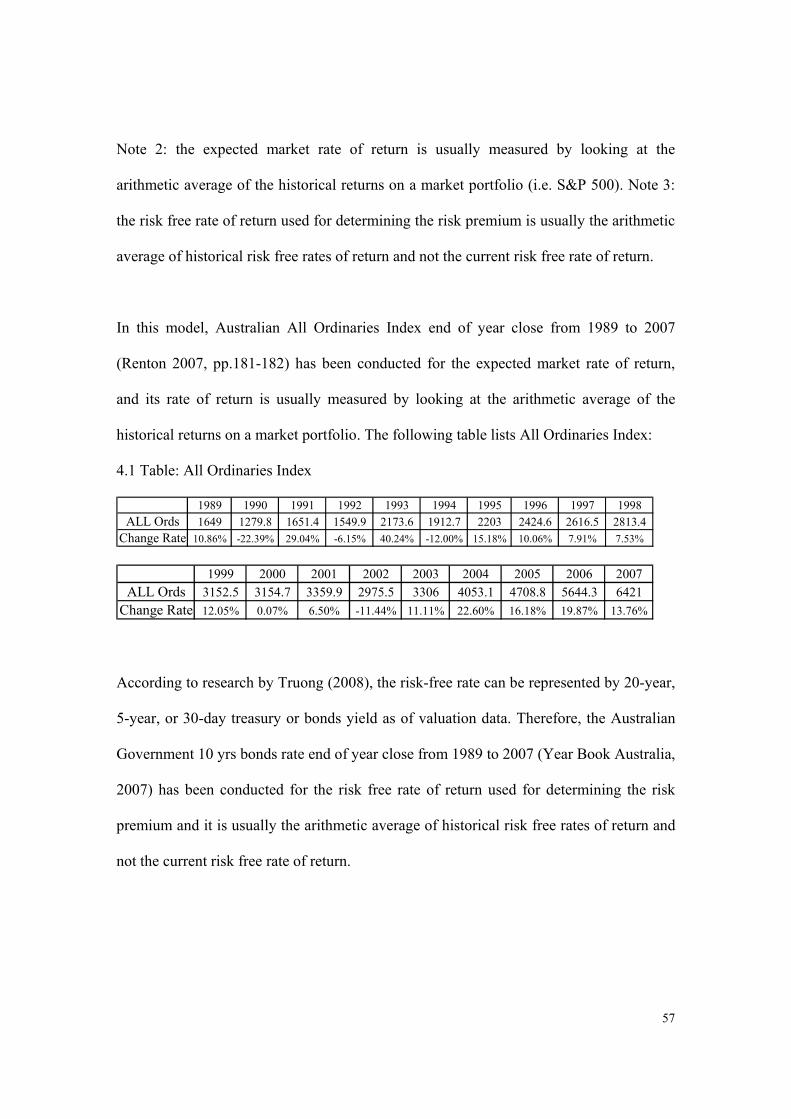
In this model, Australian All Ordinaries Index end of year close from 1989 to 2007

(Renton 2007, pp.181-182) has been conducted for the expected market rate of return,

and its rate of return is usually measured by looking at the arithmetic average of the

historical returns on a market portfolio. The following table lists All Ordinaries Index:

4.1 Table: All Ordinaries Index

1989 1990 1991 1992 1993 1994 1995 1996 1997 1998ALL Ords 1649 1279.8 1651.4 1549.9 2173.6 1912.7 2203 2424.6 2616.5 2813.4

Change Rate 10.86% -22.39% 29.04% -6.15% 40.24% -12.00% 15.18% 10.06% 7.91% 7.53%

1999 2000 2001 2002 2003 2004 2005 2006 2007ALL Ords 3152.5 3154.7 3359.9 2975.5 3306 4053.1 4708.8 5644.3 6421

Change Rate 12.05% 0.07% 6.50% -11.44% 11.11% 22.60% 16.18% 19.87% 13.76%

According to research by Truong (2008), the risk-free rate can be represented by 20-year,

5-year, or 30-day treasury or bonds yield as of valuation data. Therefore, the Australian

Government 10 yrs bonds rate end of year close from 1989 to 2007 (Year Book Australia,

2007) has been conducted for the risk free rate of return used for determining the risk

premium and it is usually the arithmetic average of historical risk free rates of return and

not the current risk free rate of return.

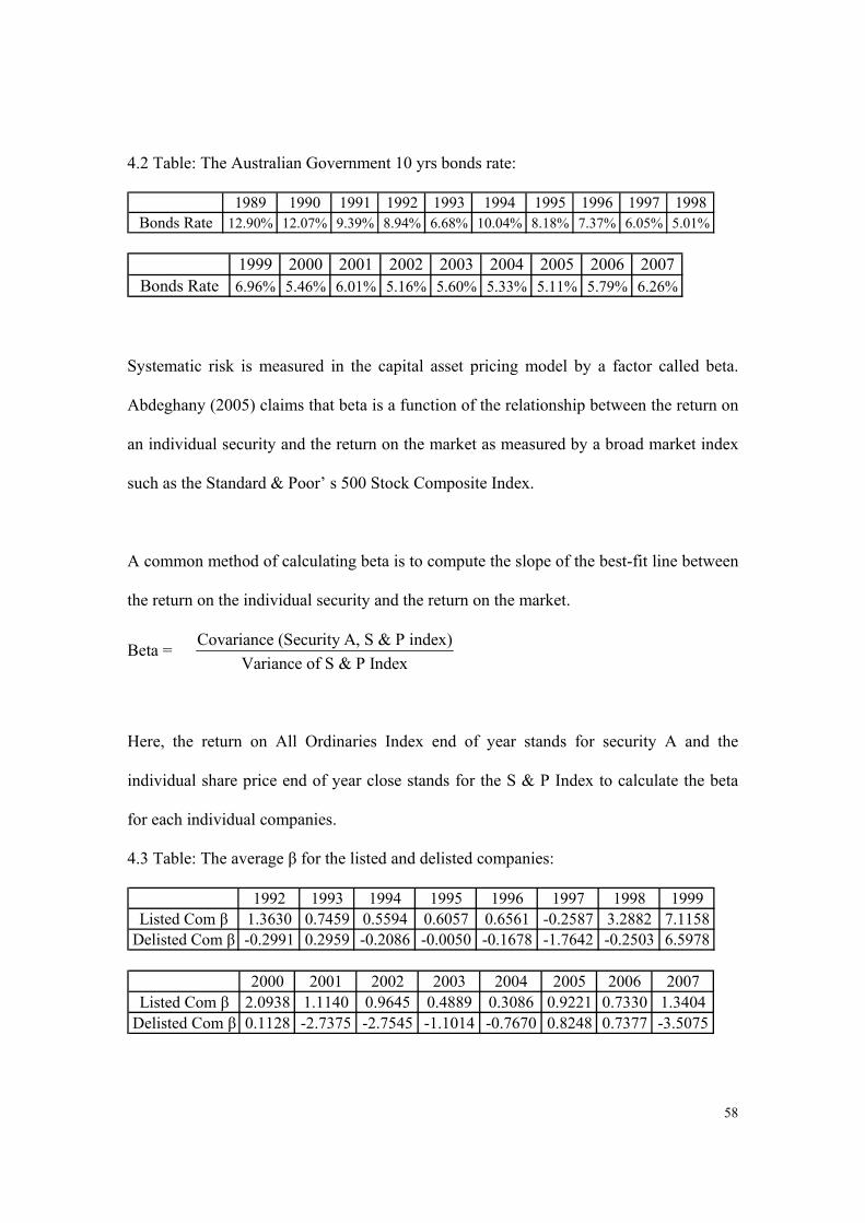
58

4.2 Table: The Australian Government 10 yrs bonds rate:

1989 1990 1991 1992 1993 1994 1995 1996 1997 1998Bonds Rate 12.90% 12.07% 9.39% 8.94% 6.68% 10.04% 8.18% 7.37% 6.05% 5.01%

1999 2000 2001 2002 2003 2004 2005 2006 2007Bonds Rate 6.96% 5.46% 6.01% 5.16% 5.60% 5.33% 5.11% 5.79% 6.26%

Systematic risk is measured in the capital asset pricing model by a factor called beta.

Abdeghany (2005) claims that beta is a function of the relationship between the return on

an individual security and the return on the market as measured by a broad market index

such as the Standard & Poor’ s 500 Stock Composite Index.

A common method of calculating beta is to compute the slope of the best-fit line between

the return on the individual security and the return on the market.

Beta = Covariance (Security A, S & P index)

Variance of S & P Index

Here, the return on All Ordinaries Index end of year stands for security A and the

individual share price end of year close stands for the S & P Index to calculate the beta

for each individual companies.

4.3 Table: The average β for the listed and delisted companies:

1992 1993 1994 1995 1996 1997 1998 1999Listed Com β 1.3630 0.7459 0.5594 0.6057 0.6561 -0.2587 3.2882 7.1158

Delisted Com β -0.2991 0.2959 -0.2086 -0.0050 -0.1678 -1.7642 -0.2503 6.5978

2000 2001 2002 2003 2004 2005 2006 2007Listed Com β 2.0938 1.1140 0.9645 0.4889 0.3086 0.9221 0.7330 1.3404

Delisted Com β 0.1128 -2.7375 -2.7545 -1.1014 -0.7670 0.8248 0.7377 -3.5075

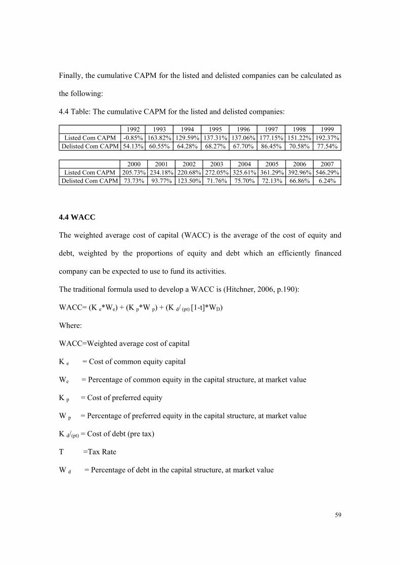
59

Finally, the cumulative CAPM for the listed and delisted companies can be calculated as

the following:

4.4 Table: The cumulative CAPM for the listed and delisted companies:

1992 1993 1994 1995 1996 1997 1998 1999Listed Com CAPM -0.85% 163.82% 129.59% 137.31% 137.06% 177.15% 151.22% 192.37%

Delisted Com CAPM 54.13% 60.55% 64.28% 68.27% 67.70% 86.45% 70.58% 77.54%

2000 2001 2002 2003 2004 2005 2006 2007Listed Com CAPM 205.73% 234.18% 220.68% 272.05% 325.61% 361.29% 392.96% 546.29%

Delisted Com CAPM 73.73% 93.77% 123.50% 71.76% 75.70% 72.13% 66.86% 6.24%

4.4 WACC

The weighted average cost of capital (WACC) is the average of the cost of equity and

debt, weighted by the proportions of equity and debt which an efficiently financed

company can be expected to use to fund its activities.

The traditional formula used to develop a WACC is (Hitchner, 2006, p.190):

WACC= (K e*We) + (K p*W p) + (K d/ (pt) [1-t]*WD)

Where:

WACC=Weighted average cost of capital

K e = Cost of common equity capital

We = Percentage of common equity in the capital structure, at market value

K p = Cost of preferred equity

W p = Percentage of preferred equity in the capital structure, at market value

K d/(pt) = Cost of debt (pre tax)

T =Tax Rate

W d = Percentage of debt in the capital structure, at market value

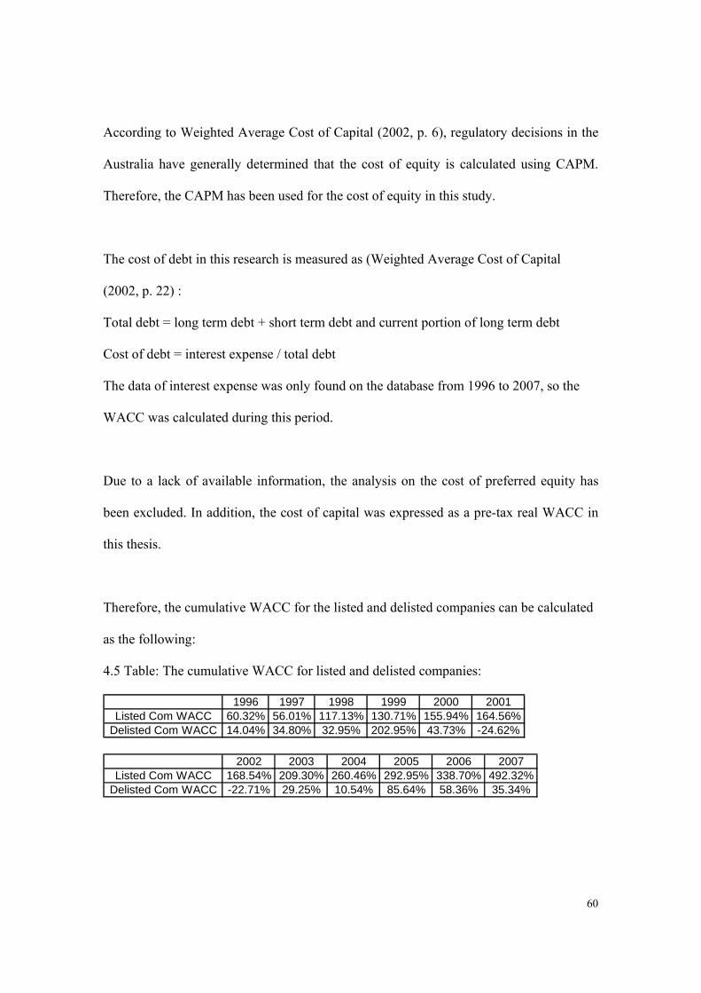
60

According to Weighted Average Cost of Capital (2002, p. 6), regulatory decisions in the

Australia have generally determined that the cost of equity is calculated using CAPM.

Therefore, the CAPM has been used for the cost of equity in this study.

The cost of debt in this research is measured as (Weighted Average Cost of Capital

(2002, p. 22) :

Total debt = long term debt + short term debt and current portion of long term debt

Cost of debt = interest expense / total debt

The data of interest expense was only found on the database from 1996 to 2007, so the

WACC was calculated during this period.

Due to a lack of available information, the analysis on the cost of preferred equity has

been excluded. In addition, the cost of capital was expressed as a pre-tax real WACC in

this thesis.

Therefore, the cumulative WACC for the listed and delisted companies can be calculated

as the following:

4.5 Table: The cumulative WACC for listed and delisted companies:

1996 1997 1998 1999 2000 2001Listed Com WACC 60.32% 56.01% 117.13% 130.71% 155.94% 164.56%

Delisted Com WACC 14.04% 34.80% 32.95% 202.95% 43.73% -24.62%

2002 2003 2004 2005 2006 2007Listed Com WACC 168.54% 209.30% 260.46% 292.95% 338.70% 492.32%

Delisted Com WACC -22.71% 29.25% 10.54% 85.64% 58.36% 35.34%

61

4.5 EVA

According to Banerjee (2000), Economic Value Added (EVA) may be defined as the net

operating profits after tax minus an appropriate charge for the opportunity cost of all

capital invested in an enterprise. Thus:

EVA = Net Operating Profit after tax – Weighted Average Cost of Capital

EVA can be rewritten as:

EVA = (ROI – WACC) x CAPITAL EMPLOYED

Therefore, in finding economic profit, the important step is to calculate net operating

profit after taxes (NOPAT).

Firstly, the earnings before interest and taxes (EBIT) and invested capital have been

selected form the database and WACC has be found form the previous work. Key

adjustments should be made, for example, by eliminating accounting distortions and

reclassifying some expenses as investments as well as subtract cash operating taxes. Due

to the data limitation, the reclassifying some expenses are not included in the adjustment.

Therefore, the EVA can be calculated using its formula. But there are lower correlations

between the EVA change rate and share price change rate, -0.00039, 0.12354 and

0.028137, respectively in the whole market, listed market and delisted market.

62

4.6 Table: The cumulative change rate of EVA for the listed and delisted companies:

1996-1997 1997-1998 1998-1999 1999-2000 2000-2001 2001-2002Listed Com Change Rate EVA -27.27% 32.45% 18.20% 136.22% 0.11% -19.94%

Delisted Com Change Rate EVA 97.30% -20.12% 30.88% 29.91% -24.37% -19.14%

2002-2003 2003-2004 2004-2005 2005-2006 2006-2007Listed Com Change Rate EVA -32.74% 57.62% 74.00% 12.65% -7.04%

Delisted Com Change Rate EVA 64.63% -52.03% 161.44% -48.58% -96.23%

4.6 P/E ratio

The P/E ratio formula is set as the following (Price-Earnings-Ratio, 2007):

P/E ratio = Price per Share

Annual Earning per Share

The price per share is the market price of a single share of the stock;

The earnings per share are the net income of the company for the most recent 12

month period, divided by number of shares outstanding.

P/E ratio is short for the ratio of the companies share price to its per-share earning. The

listed companies and delisted companies have been chosen to calculate the P/E ratio. In

the EPS calculation, the weighted average number of shares outstanding over the

reporting term has been used, in order to get more accurate EPS. It is very interesting

from the following table; there are bigger different P/E ratios for listed companies from

6.52 to 30.53 and the slight different for the delisted companies between 0.69 and 2.05.

However, both of them exist the higher correlation with the share price change rate, 0.53

and 0.64, respectively in the listed companies and in the delisted companies.

63

4.7 Table: The cumulative change rate of P/E rations for the listed and delisted companies:

1990-1991 1991-1992 1992-1993 1993-1994 1994-1995 1995-1996 1996-1997 1997-1998 1998-1999Listed Com 23.16% -3.24% 98.51% -21.35% -12.76% 70.11% 52.84% -60.61% 10.92%

Delisted Com 0.88% 35.47% -17.05% 11.29% 79.42% 7.63% -33.01% 3.01%

1999-2000 2000-2001 2001-2002 2002-2003 2003-2004 2004-2005 2005-2006 2006-2007Listed Com -51.16% 69.42% -36.47% -0.18% 60.22% -8.87% 123.25% -25.75%

Delisted Com -8.77% -3.83% 4.79% 12.75% 53.74% 8.19% 2.48% 25.67%

4.7 DCF

There are four different DCF methods depending on the financing schedule present. They

are: flows to equity approach (FTE), adjusted present value approach (APV), weighted

average cost of capital approach (WACC) and total cash flow approach (TCF). In this

thesis, flows to equity approach will be used to evaluate the energy company’s

performance in the Australia.

Middleton describes (2008) that discounted cash flow tries to calculate the value of a

company today, depending on projections of much money it’s going to make in the future.

The ten listed energy companies (CEY, ERA, HED-NZ, OSH, STO, WPL, NHC, AZA,

BNT and PVE) and five delisted energy companies (BSO, CHL, NGC-NZ, NVS and

OCA) have been selected to calculate the company’s fair value using DCF. Let’s assume

that the companies are keeping strong marketing channels, outstanding growth, efficient

factories and reasonable competitive position. So, the research will project cash flows for

the next five years of business.

64

We have decided to estimate the free cash flow that the selected companies will produce

over the next five years. Forecasting the companies’ revenue is the most important

assumption one that decides the company’s free cash flow.

We have got the company average revenue growth rate at 15% for the past 10 years and

the companies will keep at 10% in the future five years. We then calculate the past 10

years average operating costs margin of 65%, in order to derive the operating costs. We

assume that the net investment is 10% of the revenue and the working capital has

increased by 10% each year.

So the free cash flow can be calculated as the following (Benninga 2000, p. 65):

Free Cash Flow = Sales Revenue – Operating Costs – Taxes – Net Investment – Change

in Working Capital

And we should calculate the terminal value approach that involves making some

assumptions about long-term cash flow growth (Benninga 2000, p.70).

Terminal Value = Final Projected Year Cash Flow X (1+Long-Term Cash Flow Growth Rate)

(WACC – Long-Term Cash Flow Growth Rate

In this formula, let’s assume that the company’s cash flows will grow in perpetuity by 4%

per year.

Then the enterprise value of the firms becomes the discounted value of the firm’s

projected FCF plus its terminal value (Benninga 2000, p. 72)

Enterprise value= FCF1/ (1+WACC) 1+FCF2/ (1+WACC) 2+……………………...

65

FCF5/ (1+WACC) 5+Year 5 terminal value/ (1+WACC)

After that, we should deduct its net debt from the value to calculate the companies’ fair

value of equity. Finally, the companies’ share price can be calculated by the enterprise

value of equity divided by the shares outstanding.

4.8 Table: The cumulative forecasting share price change rate for the listed and delisted companies:

1996 -1997 1997-1998 1998 -1999 1999 -2000 2000 -2001 2001-2002Listed Com 29.99% -44.99% 62.36% -38.06% 63.19% -0.65%

Delisted Com -48.15% -1317.86% -174.19% 17.00% 82.43% -3.52%

2002-2003 2003 -2004 2004 -2005 2005 -2006 2006 -2007Listed Com -79.45% 359.44% -49.34% 34.93% 172.01%

Delisted Com 9.79% 9.97% -48.65% -42.41%

4.8 MateCapitalism

To examines the MetaCapitalism: the e-business revolution and the design of 21st

century companies and markets and its role of efficiency changes to capital, technology

and labour in the private and public sectors, and their overall impact on global financial

markets.

MetaCapitalism Equation The MetaCapitalism equation is used as a means of reducing the strategy to a measurable

index. The core tenets of MetaCapitalism are de capitalisation, outsourcing and

downsizing and these can be measured by PP&E, NWC and NOE (Means & Schneider,

2000). Measure a firm’s level of MetaCapitalisation by calculating its composite change

value over time, based on:

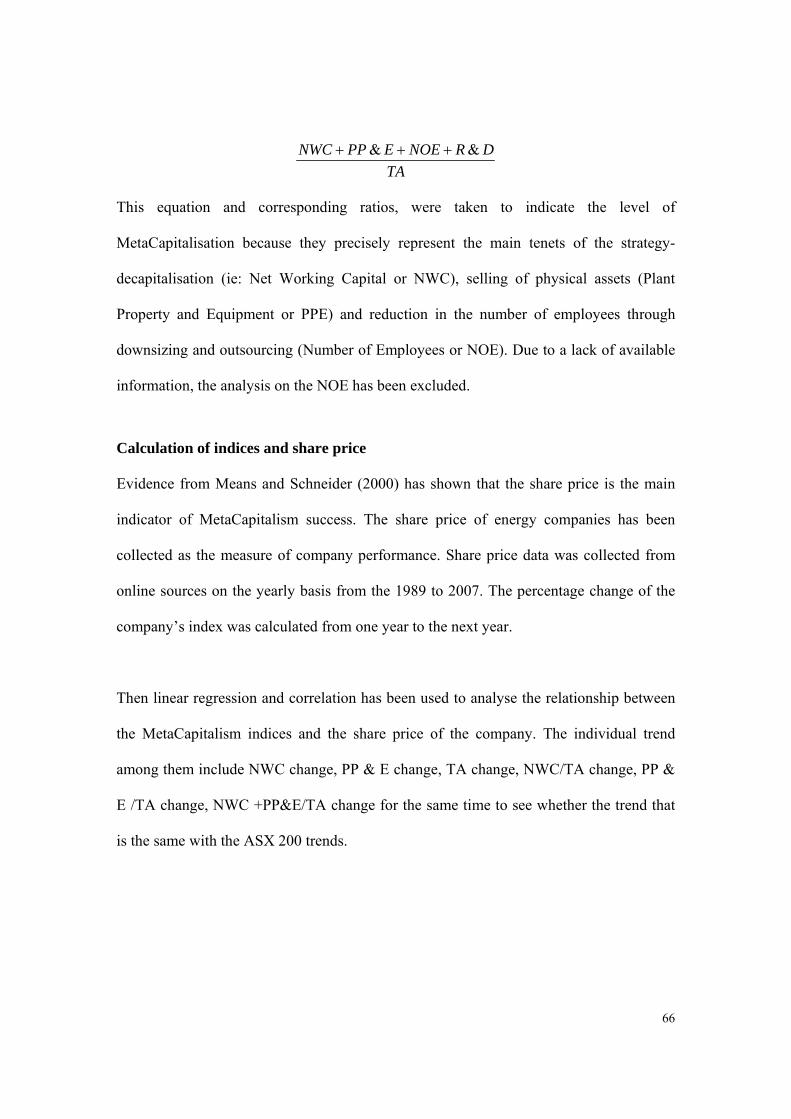
66

& &NWC PP E NOE R D

TA

This equation and corresponding ratios, were taken to indicate the level of

MetaCapitalisation because they precisely represent the main tenets of the strategy-

decapitalisation (ie: Net Working Capital or NWC), selling of physical assets (Plant

Property and Equipment or PPE) and reduction in the number of employees through

downsizing and outsourcing (Number of Employees or NOE). Due to a lack of available

information, the analysis on the NOE has been excluded.

Calculation of indices and share price Evidence from Means and Schneider (2000) has shown that the share price is the main

indicator of MetaCapitalism success. The share price of energy companies has been

collected as the measure of company performance. Share price data was collected from

online sources on the yearly basis from the 1989 to 2007. The percentage change of the

company’s index was calculated from one year to the next year.

Then linear regression and correlation has been used to analyse the relationship between

the MetaCapitalism indices and the share price of the company. The individual trend

among them include NWC change, PP & E change, TA change, NWC/TA change, PP &

E /TA change, NWC +PP&E/TA change for the same time to see whether the trend that

is the same with the ASX 200 trends.

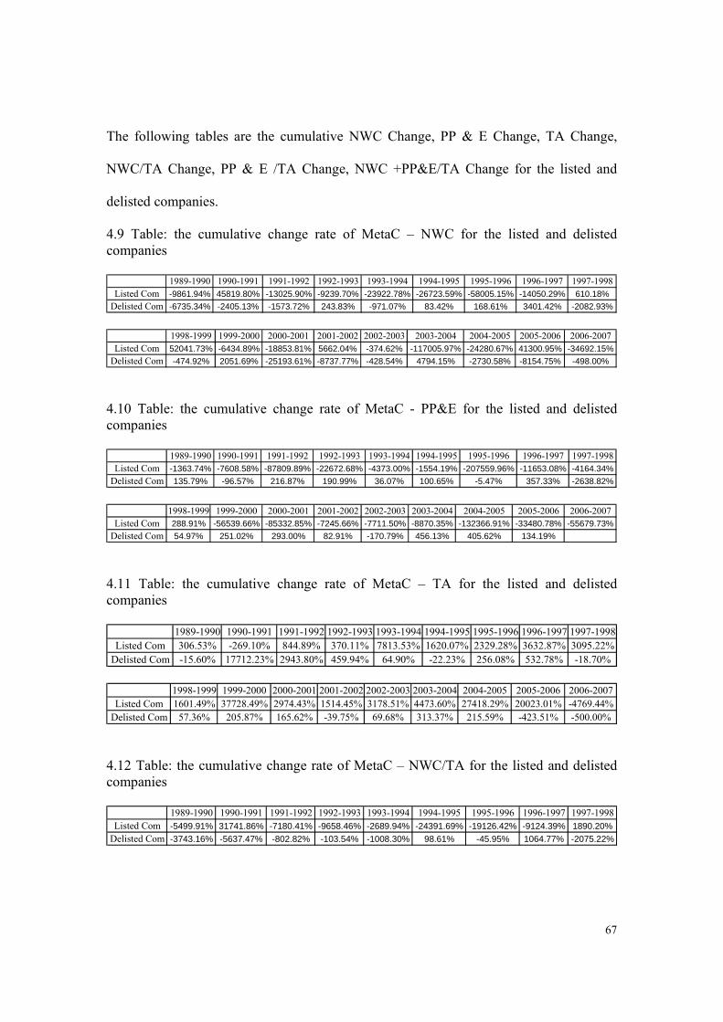
67

The following tables are the cumulative NWC Change, PP & E Change, TA Change,

NWC/TA Change, PP & E /TA Change, NWC +PP&E/TA Change for the listed and

delisted companies.

4.9 Table: the cumulative change rate of MetaC – NWC for the listed and delisted companies

1989-1990 1990-1991 1991-1992 1992-1993 1993-1994 1994-1995 1995-1996 1996-1997 1997-1998Listed Com -9861.94% 45819.80% -13025.90% -9239.70% -23922.78% -26723.59% -58005.15% -14050.29% 610.18%

Delisted Com -6735.34% -2405.13% -1573.72% 243.83% -971.07% 83.42% 168.61% 3401.42% -2082.93%

1998-1999 1999-2000 2000-2001 2001-2002 2002-2003 2003-2004 2004-2005 2005-2006 2006-2007Listed Com 52041.73% -6434.89% -18853.81% 5662.04% -374.62% -117005.97% -24280.67% 41300.95% -34692.15%

Delisted Com -474.92% 2051.69% -25193.61% -8737.77% -428.54% 4794.15% -2730.58% -8154.75% -498.00%

4.10 Table: the cumulative change rate of MetaC - PP&E for the listed and delisted companies

1989-1990 1990-1991 1991-1992 1992-1993 1993-1994 1994-1995 1995-1996 1996-1997 1997-1998Listed Com -1363.74% -7608.58% -87809.89% -22672.68% -4373.00% -1554.19% -207559.96% -11653.08% -4164.34%

Delisted Com 135.79% -96.57% 216.87% 190.99% 36.07% 100.65% -5.47% 357.33% -2638.82%

1998-1999 1999-2000 2000-2001 2001-2002 2002-2003 2003-2004 2004-2005 2005-2006 2006-2007Listed Com 288.91% -56539.66% -85332.85% -7245.66% -7711.50% -8870.35% -132366.91% -33480.78% -55679.73%

Delisted Com 54.97% 251.02% 293.00% 82.91% -170.79% 456.13% 405.62% 134.19%

4.11 Table: the cumulative change rate of MetaC – TA for the listed and delisted companies

1989-1990 1990-1991 1991-1992 1992-1993 1993-1994 1994-1995 1995-1996 1996-1997 1997-1998Listed Com 306.53% -269.10% 844.89% 370.11% 7813.53% 1620.07% 2329.28% 3632.87% 3095.22%

Delisted Com -15.60% 17712.23% 2943.80% 459.94% 64.90% -22.23% 256.08% 532.78% -18.70%

1998-1999 1999-2000 2000-2001 2001-2002 2002-2003 2003-2004 2004-2005 2005-2006 2006-2007Listed Com 1601.49% 37728.49% 2974.43% 1514.45% 3178.51% 4473.60% 27418.29% 20023.01% -4769.44%

Delisted Com 57.36% 205.87% 165.62% -39.75% 69.68% 313.37% 215.59% -423.51% -500.00%

4.12 Table: the cumulative change rate of MetaC – NWC/TA for the listed and delisted companies

1989-1990 1990-1991 1991-1992 1992-1993 1993-1994 1994-1995 1995-1996 1996-1997 1997-1998Listed Com -5499.91% 31741.86% -7180.41% -9658.46% -2689.94% -24391.69% -19126.42% -9124.39% 1890.20%

Delisted Com -3743.16% -5637.47% -802.82% -103.54% -1008.30% 98.61% -45.95% 1064.77% -2075.22%

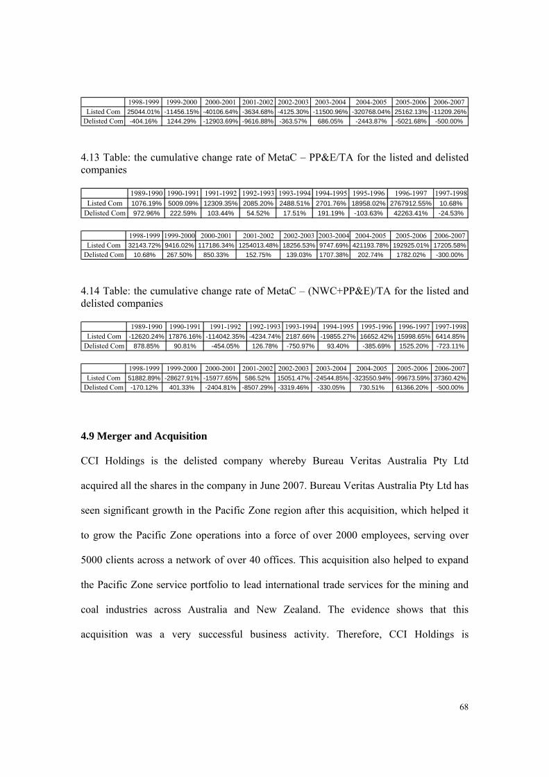
68

1998-1999 1999-2000 2000-2001 2001-2002 2002-2003 2003-2004 2004-2005 2005-2006 2006-2007Listed Com 25044.01% -11456.15% -40106.64% -3634.68% -4125.30% -11500.96% -320768.04% 25162.13% -11209.26%

Delisted Com -404.16% 1244.29% -12903.69% -9616.88% -363.57% 686.05% -2443.87% -5021.68% -500.00%

4.13 Table: the cumulative change rate of MetaC – PP&E/TA for the listed and delisted companies

1989-1990 1990-1991 1991-1992 1992-1993 1993-1994 1994-1995 1995-1996 1996-1997 1997-1998Listed Com 1076.19% 5009.09% 12309.35% 2085.20% 2488.51% 2701.76% 18958.02% 2767912.55% 10.68%

Delisted Com 972.96% 222.59% 103.44% 54.52% 17.51% 191.19% -103.63% 42263.41% -24.53%

1998-1999 1999-2000 2000-2001 2001-2002 2002-2003 2003-2004 2004-2005 2005-2006 2006-2007Listed Com 32143.72% 9416.02% 117186.34% 1254013.48% 18256.53% 9747.69% 421193.78% 192925.01% 17205.58%

Delisted Com 10.68% 267.50% 850.33% 152.75% 139.03% 1707.38% 202.74% 1782.02% -300.00%

4.14 Table: the cumulative change rate of MetaC – (NWC+PP&E)/TA for the listed and delisted companies

1989-1990 1990-1991 1991-1992 1992-1993 1993-1994 1994-1995 1995-1996 1996-1997 1997-1998Listed Com -12620.24% 17876.16% -114042.35% -4234.74% 2187.66% -19855.27% 16652.42% 15998.65% 6414.85%

Delisted Com 878.85% 90.81% -454.05% 126.78% -750.97% 93.40% -385.69% 1525.20% -723.11%

1998-1999 1999-2000 2000-2001 2001-2002 2002-2003 2003-2004 2004-2005 2005-2006 2006-2007Listed Com 51882.89% -28627.91% -15977.65% 586.52% 15051.47% -24544.85% -323550.94% -99673.59% 37360.42%

Delisted Com -170.12% 401.33% -2404.81% -8507.29% -3319.46% -330.05% 730.51% 61366.20% -500.00%

4.9 Merger and Acquisition

CCI Holdings is the delisted company whereby Bureau Veritas Australia Pty Ltd

acquired all the shares in the company in June 2007. Bureau Veritas Australia Pty Ltd has

seen significant growth in the Pacific Zone region after this acquisition, which helped it

to grow the Pacific Zone operations into a force of over 2000 employees, serving over

5000 clients across a network of over 40 offices. This acquisition also helped to expand

the Pacific Zone service portfolio to lead international trade services for the mining and

coal industries across Australia and New Zealand. The evidence shows that this

acquisition was a very successful business activity. Therefore, CCI Holdings is

69

considered as a subject company and contrived to illustrate the guideline merger and

acquisition of the market approach.

Summary Description of CCI Holdings

According to Australian companies’ information and details (2008), CCI Holdings was

providing a range of services, including equipment monitoring, engineering,

superintending and laboratory services to the coal industry and to other industries, such as

oil and gas, steel, petrochemical and construction. Operations are conducted from a

leased facility located in Sydney. As of the company’s fiscal year ended December 31,

2006, CCI Holdings reported operating and net income of $ 1.5 million and $ 2.7 million,

respectively, on revenues of $ 59 million.

Australian Economic Outlook

Odell (2007) outlines that the Australian real GDP in 2006 increased at a 2.7% compared

to 2005. Consumer price index (CPI) and producer price index (PPI) which are key

indicators of inflation in the Australian economy remained steady between in 2005 and in

2006. Unemployment rates also slightly decreased during the same periods, and its

unemployment is at a 28-year low at 4.1 per cent. This evidence indicates that the

Australian economy has developed very well and the governments efficiently control the

CPI and the unemployment rate index. The economic outlook for the Australia at the end

of 2006 appeared to be optimistic for the CCI Holdings.

Energy Industry Outlook

70

Odell (2007) claims that the Australian energy sector has undergone significant change

over the past twenty-five years and its growth in energy consumption has closely

followed that in Australia’s total output or GDP trend. Australia is a major exporter and

user of coal, the burning of which creates carbon dioxide. Consequently, in 2000

Australia was the fifth highest emitter of greenhouse gases per capita in the developed

world when emissions from land clearing are not included. “Australia’s renewable energy

industries cover numerous energy sources and scales of operation, and currently

contribute about 5.9% of Australia’s total energy supply” (Haralambopoulos 2003, p. 49).

Fundamental Position of the Company

CCI Holdings was incorporated in 1997 and it is in a NSW based ASX listed company.

The company’s primary line is to supply technical services to the Australian and

international coal industries. The following will explain the company fundamental

position.

History

CCI Holdings provides a range of services to the Australian and international coal

industries. While the coal industry is the company major focus, the company’s services

are utilised by a number of large industries such as oil and gas, steel, petrochemical and

construction (CCI Holdings Limited, 2007).

CCI Holdings listed on the Australian Stock Exchange (ASX) in 1991, and has

experienced rapid growth over the last ten years. The company has approximately 1700

71

shareholders who have enjoyed substantial dividends over the years. The company is old

fashioned in that it is focused on earning profits, paying tax and rewarding shareholders

(CCI Holdings Limited, 2007).

Employees

CCI Holdings employs more than 600 people world wide, many whom have worked for

the company for more than ten years. The staff has a real interest in ensuring the

continued success of CCI Holdings (CCI Holdings Limited, 2007).

CCI Holdings’ organisational structure remained the fixed pattern; the key management

personnel consisted of (CCI Holdings Limited, 2007):

Mr Peter EJ Murray (Chairman, Director)

Mr David Butel (Director, CEO)

Mr Brian Milton (CFO)

Mr Sean G.S Hughes (Independent Director, Executive Director, Non Exec. Director)

Mr Robin Chenery (Independent Director, Non Exec. Director)

Mr Brendan Thomas Birthistle (Independent Director, Non Exec. Director)

Capitalisation and Ownership

The major top five shareholders of CCI Holdings (as at 21 February 2007) are (CCI

Holdings Limited, 2007):

AUSTRALIAN LABORATORY SERVICES PTY LTD 21.52 %

IMPERIAL PACIFIC FUND MANAGERS PTY LTD 13.38 %

72

MR SEAN HUGHES + MRS ELIZABETH HUGHES 12.12 %

LONDON CITY EQUITIES LTD 2.36 %

HGL GROUP PTY LTD 2.26 %

Dividend Policy

Dividends are generally paid to shareholders of CCI Holdings biannually. The

shareholders may continue to take the full dividend in cash or may reinvest all or part of

the dividend into further shares under the CCI Dividend Reinvestment Plan (CCI

Holdings Limited, 2007).

Selected Market Data

We start to value CCI Holdings by using the guideline merger and acquisition method of

the market approach. To establish a reasonable basis for comparison between the subject

company and the selected guideline companies, market data was collected by the

following criteria (Pratt, 2001, pp191):

Similar business description or market;

Revenues between $ 1 million and $750 million;

Positive operating earnings for the latest reported fiscal year-end;

Positive cash flow for the latest reported fiscal year-end; and

Business located in the Australia,

The five companies were selected by the criteria of selected guideline companies, and the

following is brief description of each selected guideline transactions:

73

1. Magellan Petroleum Australian Limited (MAG)

Magellan Petroleum Australian Limited delisted on 3 July 2006. Magellan Petroleum

Corporation acquired Magellan Petroleum Australian Limited and it was successful with

an offer of 7.5 Magellan Petroleum Corporation shares and $1.00 cash for every 10

Magellan Petroleum Australian Limited shares (Magellan Petroleum Australian Limited,

2008).

Magellan Petroleum Australian Limited engages in the sale of oil and gas and exploration

and development of oil and gas reserves. In addition, it holds interest in various oil and

gas properties in New Zealand and the United Kingdom. The company was founded in

1957 and is based in Hartford, Connecticut (Magellan Petroleum Australian Limited,

2008).

2. Excel Coal Limited (EXL)

Peabody Energy Corporation acquired all of the shares in Excel for $9.50 per share on 11

April 2006. Excel Coal Limited invests in and manages coalmines in New South Wales

and Queensland and is based in Sydney, Australia. It produces a diverse range of

products including thermal coal, hard coking coal, semi-hard coking coal and coke, most

of which is sold under contract to major customers in both the export and domestic

markets. The company holds interests in the production of metallurgical coke and

industrial minerals and holds certain other mining related investments (Excel Coal

Limited, 2008).

74

3. Oil Company of Australia Limited (OCA)

Origin Energy Limited was successful with a cash offer of $4.25 cash per share

compulsory acquired Oil Company of Australia Limited (Oil Company of Australia

Limited, 2008).

4. Novus Petroleum Limited (NVS)

Medco Energy (Australia) Pty Ltd was successful with a cash offer of $1.90 per share

compulsory acquired Novus Petroleum Limited on 13 July 2004. Novus Petroleum

Limited is an Australian upstream petroleum company that focused on the exploration

and the production of crude oil, natural gas and associated liquids. The Company’s

production activities are carried out in four countries: Australia, United States, Oman and

Indonesia. Active exploration is also undertaken in all these countries in addition to

Pakistan and the United Arab Emirates (Novus Petroleum Limited, 2008).

5. NGC Holdings Limited (NGC – NZ)

Natural Gas Corporation Holdings Ltd. (NGC) is a New Zealand-based energy

infrastructure and service company. The Company has interests in natural gas and

liquefied petroleum gas (LPG) transportation, sales and energy marketing. NGC’s energy

sales business is involved in the acquisition, processing and sales of natural gas and

associated by-products, including LPG. It owns approximately 55,000 gas meters, and

holds a market share of approximately 24% of total gas meter installations in New

Zealand (NGC Holdings Limited, 2008).

75

CHAPTER FIVE

DATA ANALYSIS

76

5.1 Introduction

Simple linear regression and correlation have been conducted to analyse the relationship

between the business evaluation methods and the share price. Correlation analysis is a

group of techniques to measure the association between two variables. In addition, the

linear regression graph and t-test were used to assess whether the means of two groups

are statistically different from each other. The main purpose of using simple linear

regression is to establish the strength of the link between the business evaluation methods

and the share price.

5.2 Data analysis

Evidence from Hill (2001, p. 20) shows that regression analysis is a statistical tool for the

investigation of relationships between variables. Usually, the investigator seeks to

ascertain the causal effect of one variable upon another. This evidence shows that the

dependent variables are those that are observed to change in response to the independent

variables. The independent variables are those that are deliberately manipulated to invoke

a change in the dependent variables.

Regression analysis has been used to develop an equation (a linear regression line) for

predicting a value of the dependent variables given a value of the independent variable.

The simple regression equation is given by (Linear Regression and Excel, 2008):

Y = a + b X

77

Where X is the independent variable, Y is the dependent variable, a is the intercept and b

is the slope of the line. For every fixed value of X, the E’S are assumed to be independent

random quantities normally distributed with mean zero.

In this study, the main purpose is to establish the strength of the link between the

business evaluation methods and the share prices, so the simple regression analysis has

been used to analyse their relationship. The business evaluation methods are the predicted

value, so it is termed the dependent variable. The share prices are actual value and it is

termed the independent variable. The following steps are to describe the regression index

and graph, in order to explore the relationship between them.

5.3 The regression between business evaluation methods and share prices in the

whole market

The purpose of this part is to analyse the regression between the different business

evaluation methods and the share price in the whole market. CAPM, WACC, EVA, P/E

ratio, DCF, MetaC – NWC, MetaC - PP&E, MetaC - TA, MetaC - NWC/TA, MetaC -

PP&E/TA , MetaC (NWC+PP&E)/TA included in business evaluation methods.

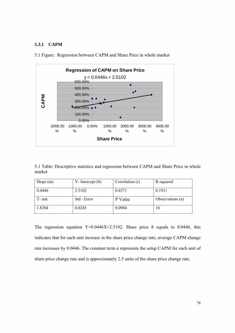
78

5.3.1 CAPM

5.1 Figure: Regression between CAPM and Share Price in whole market

Regression of CAPM on Share Price

y = 0.0446x + 2.5102

0.00%

100.00%

200.00%

300.00%

400.00%

500.00%

600.00%

-2000.00%

-1000.00%

0.00% 1000.00%

2000.00%

3000.00%

4000.00%

Share Price

CA

PM

5.1 Table: Descriptive statistics and regression between CAPM and Share Price in whole market

The regression equation Y=0.0446X+2.5102. Share price b equals to 0.0446, this

indicates that for each unit increase in the share price change rate, average CAPM change

rate increases by 0.0446. The constant term a represents the setup CAPM for each unit of

share price change rate and is approximately 2.5 units of the share price change rate.

Slope (m) Y- Intercept (b) Correlation (r) R-squared

0.0446 2.5102 0.4371 0.1911

T- stat Std - Error P Value Observations (n)

1.8204 0.0245 0.0904 16

79

R2 =19.11% is moderately small. It tells us that 19.11% of the variation in percentage of

CAPM change rate is explained by the independent variable share price. Furthermore, it

is implied that 81.89% of the variation in the percentage of CAPM change rate remains

unexplained. Overall, the model provides a poor fit.

P Value with a value ranges from zero to one - the probability of observing a test statistic

that is as extreme as or more extreme than currently observed assuming that the null

hypothesis is true. Convention is that we accept a P value of 0.05 or below as being

statistically significant. P Value 0.0904 is more than 0.05, so it is not accepted as

statistically significant. The standard error 0.0245 balances the dispersion associated with

the underlying population and the error associated with the sampling process.

Tests of Hypotheses

Hypotheses:

H0: μ =0 (there is no linear relationship) n=16

H1: μ ≠0 (there is a linear relationship) (two – tailed test)

Significance level: α = 0.05 tcrit =t α/2, n-1df=

t 0.025, 15df=2.131

Decision rule: Reject H0 if t calc >2.131 or if t calc < -2.131

Do not reject H0 if -2.131 ≤ t calc ≤ 2.131

Test statistic: ˆ

ˆ

b

bt

s

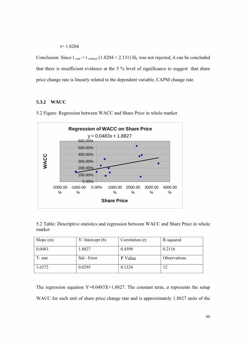
80

t= 1.8204

Conclusion: Since t calc < t critical (1.8204 < 2.131) H0 was not rejected, it can be concluded

that there is insufficient evidence at the 5 % level of significance to suggest that share

price change rate is linearly related to the dependent variable, CAPM change rate.

5.3.2 WACC

5.2 Figure: Regression between WACC and Share Price in whole market

Regression of WACC on Share Price

y = 0.0483x + 1.8827

0.00%

100.00%

200.00%

300.00%

400.00%

500.00%

600.00%

-2000.00%

-1000.00%

0.00% 1000.00%

2000.00%

3000.00%

4000.00%

Share Price

WA

CC

5.2 Table: Descriptive statistics and regression between WACC and Share Price in whole market

The regression equation Y=0.0483X+1.8827. The constant term, a represents the setup

WACC for each unit of share price change rate and is approximately 1.8827 units of the

Slope (m) Y- Intercept (b) Correlation (r) R-squared

0.0483 1.8827 0.4599 0.2116

T- stat Std - Error P Value Observations

1.6372 0.0295 0.1324 12

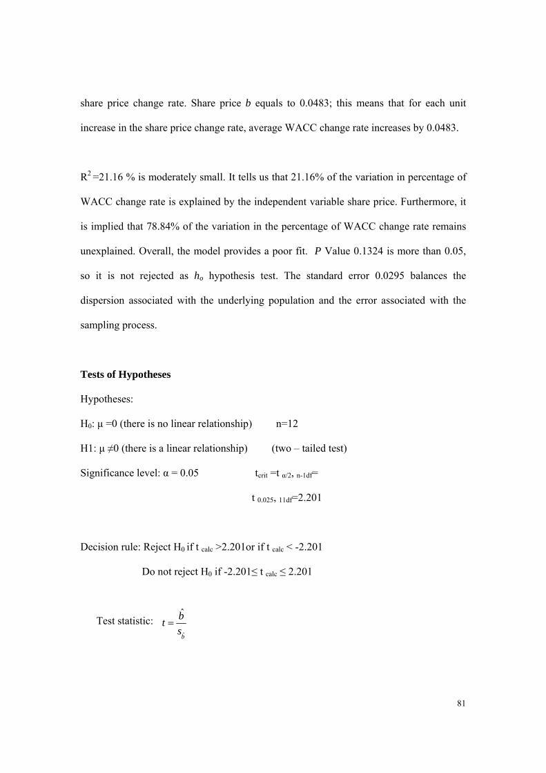
81

share price change rate. Share price b equals to 0.0483; this means that for each unit

increase in the share price change rate, average WACC change rate increases by 0.0483.

R2 =21.16 % is moderately small. It tells us that 21.16% of the variation in percentage of

WACC change rate is explained by the independent variable share price. Furthermore, it

is implied that 78.84% of the variation in the percentage of WACC change rate remains

unexplained. Overall, the model provides a poor fit. P Value 0.1324 is more than 0.05,

so it is not rejected as ho hypothesis test. The standard error 0.0295 balances the

dispersion associated with the underlying population and the error associated with the

sampling process.

Tests of Hypotheses

Hypotheses:

H0: μ =0 (there is no linear relationship) n=12

H1: μ ≠0 (there is a linear relationship) (two – tailed test)

Significance level: α = 0.05 tcrit =t α/2, n-1df=

t 0.025, 11df=2.201

Decision rule: Reject H0 if t calc >2.201or if t calc < -2.201

Do not reject H0 if -2.201≤ t calc ≤ 2.201

Test statistic:

ˆ

ˆ

b

bt

s

82

t= 1.6372

Conclusion: Since t calc < t critical (1.6372 < 2.201) H0 was not rejected, it can be concluded

that there is insufficient evidence at the 5 % level of significance to suggest that share

price change rate is linearly related to the dependent variable, WACC change rate.

5.3.3 EVA

5.3 Figure: Regression between EVA and Share Price in whole market

Regression of EVA on Share Pricey = -3E-05x + 0.3348

-150.00%

-100.00%

-50.00%

0.00%

50.00%

100.00%

150.00%

200.00%

250.00%

300.00%

-2000.00%

-1000.00%

0.00% 1000.00%

2000.00%

3000.00%

4000.00%

Share Price

EV

A

5.3 Table: Descriptive statistics and regression between EVA and Share Price in whole market

Slope (m) Y- Intercept (b) Correlation (r) R-squared

-3E-0.5 0.3348 -0.0004 0

T- stat Std - Error P Value Observations

-0.0012 0.0241 0.9991 11

83

The regression equation Y=-3E-0.5X+0.3348. The b is very small -3E-0.5 and represents

that each unit increase in the share price change rate, average EVA change rate decreases

by -3E-0.5. The constant term a represents the setup EVA for each unit of share price

change rate and is approximately 0.3348 units of the share price change rate.

R2 =0, It tells us that 0% of the variation in percentage of EVA change rate is explained

by the independent variable share price. Furthermore, it is implied that 100% of the

variation in the percentage of EVA change rate remains unexplained. Overall, the model

provides nothing. P Value 0.9991 is nearly 100%, so it is not accepted as statistically

significant. The standard error 0.0241 measured the dispersion associated with the

underlying population and the error associated with the sampling process.

Tests of Hypotheses

Hypotheses:

H0: μ =0 (there is no linear relationship) n=11

H1: μ ≠0 (there is a linear relationship) (two – tailed test)

Significance level: α = 0.05 tcrit =t α/2, n-1df=

t 0.025, 10df=2.228

Decision rule: Reject H0 if t calc >2.228 or if t calc < -2.228

Do not reject H0 if -2.228 ≤ t calc ≤ 2.228

Test statistic:

ˆ

ˆ

b

bt

s

84

t= -0.0012

Conclusion: Since t critical ≤ t calc ≤ t critical (-2.228 < -0.0012 < 2.228) H0 was not rejected,

it can be concluded that there is insufficient evidence at the 5 % level of significance to

suggest that share price change rate is linearly related to the dependent variable, EVA

change rate.

5.3.4 P/E ratio

5.4 Figure: Regression between P/E ratio and Share Price in whole market

Regression of P/E Ratio on Share Price

y = 0.0396x - 0.1345

-150.00%

-100.00%

-50.00%

0.00%

50.00%

100.00%

150.00%

200.00%

-2000.00%

-1000.00%

0.00% 1000.00% 2000.00% 3000.00% 4000.00%

Share Price

P/E

Ra

tio

5.4 Table: Descriptive statistics and regression between P/E ratio and Share Price in

whole market

Slope (m) Y- Intercept (b) Correlation (r) R-squared

0.0396 -0.1345 0.6588 0.4339

T- stat Std - Error P Value Observations

3.3846 0.0117 0.0040 17

85

The regression equation Y=0.0396X–0.1345. Share price b equals to 0.0396, this means

that each unit increase in the share price change rate, average P/E ratio change rate

increases by 0.0396. The constant term a represents the setup P/E ratio for each unit of

share price change rate and is approximately -0.1345 units of the share price change rate.

R2 =43.39%, moderately large. It tells us that 43.39% of the variation in percentage of

P/E ratio change rate is explained by the independent variable share price. Furthermore, it

is implied that 46.61% of the variation in the percentage of P/E ratio change rate remains

unexplained. Overall, the model provides a good fit. P Value 0.0040 is smaller than 0.05,

so it is accepted as statistically significant.

Tests of Hypotheses

Hypotheses:

H0: μ =0 (there is no linear relationship) n=17

H1: μ ≠0 (there is a linear relationship) (two – tailed test)

Significance level: α = 0.05 t crit =t α/2, n-1df=

t 0.025, 16df=2.120

Decision rule: Reject H0 if t calc >2.120 or if t calc < -2.120

Do not reject H0 if -2.120 ≤ t calc ≤ 2.120

Test statistic:

t= 3.3846

ˆ

ˆ

b

bt

s

86

Conclusion: Since t calc > t critical (3.3846 > 2.120) H0 was rejected, it can be concluded

that there is sufficient sample evidence at the 5 % level of significance to suggest that

there is a stronger linear relationship between share price change rate and P/E ratio

change rate.

5.4.1 DCF

5.5 Figure: Regression between DCF and Share Price in whole market

Regression of DCF on Share Pricey = 0.2251x - 3.3351

-1500.00%

-1000.00%

-500.00%

0.00%

500.00%

1000.00%

-2000.00%

-1000.00%

0.00% 1000.00%

2000.00%

3000.00%

4000.00%

Share Price

DC

F

5.5 Table: Descriptive statistics and regression between DCF and Share Price in whole market

Slope (m) Y- Intercept (b) Correlation (r) R-squared

0.2251 -3.3351 0.6744 0.4549

T- stat Std - Error P Value Observations

2.7418 0.0821 0.0229 11

87

The regression equation Y=0.2251X-3.3351. R2 =45.49% is moderately large. It tells us

that 45.49% of the variation in percentage of DCF change rate is explained by the

independent variable share price. Furthermore, it is implied that 54.51% of the variation

in the percentage of DCF change rate remains unexplained. Overall, the model provides a

good fit.

Share price b equals to 0.2251, this meaning is for each unit increase in the share price

change rate, average DCF change rate increases by 0.2251. And DCF change rate trends

are similar with the share price change rate. The constant term a represents the setup DCF

for each unit of share price change rate and is approximately -3.3351 units of the share

price change rate.

Generally, P Value with a value ranges from zero to one. P Value 0.0229 is less than 0.05,

so the hypothesis 1 null μ=0 is rejected. The standard error 0.0821 explores the dispersion

associated with the underlying population and the error associated with the sampling

process.

Tests of Hypotheses

Hypotheses:

H0: μ =0 (there is no linear relationship) n=11

H1: μ ≠0 (there is a linear relationship) (two – tailed test)

Significance level: α = 0.05 tcrit =t α/2, n-1df=

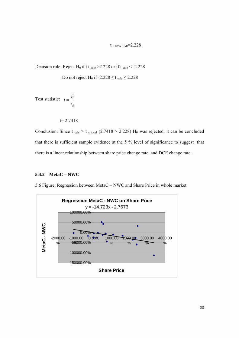
88

t 0.025, 10df=2.228

Decision rule: Reject H0 if t t calc >2.228 or if t calc < -2.228

Do not reject H0 if -2.228 ≤ t calc ≤ 2.228

Test statistic:

t= 2.7418

Conclusion: Since t calc > t critical (2.7418 > 2.228) H0 was rejected, it can be concluded

that there is sufficient sample evidence at the 5 % level of significance to suggest that

there is a linear relationship between share price change rate and DCF change rate.

5.4.2 MetaC – NWC

5.6 Figure: Regression between MetaC – NWC and Share Price in whole market

Regression MetaC - NWC on Share Pricey = -14.723x - 2.7673

-150000.00%

-100000.00%

-50000.00%

0.00%

50000.00%

100000.00%

-2000.00%

-1000.00%

0.00% 1000.00%

2000.00%

3000.00%

4000.00%

Share Price

Me

taC

- N

WC

ˆ

ˆ

b

bt

s

89

5.6 Table: Descriptive statistics and regression between MetaC – NWC and Share Price in whole market

The regression equation Y=-14.7230X-2.7673. R2 =21.77% is moderately small. It tells

us that 21.77% of the variation in percentage of MetaC–NWC change rate is explained by

the independent variable share price. Furthermore, it is implied that 78.32% of the

variation in the percentage of MetaC–NWC change rate remains unexplained. Overall,

the model provides a poor fit.

Share price b equals to -14.7230; it is clearly that each unit increases in the share price

change rate, average MetaC – NWC change rate decreases b-14.7230. P Value is 0.0513

and T-stat is -2.1061, so the test statistic has not rejected and the null hypothesis is true.

The standard error 6.9907 is bigger figure and it has shown the dispersion associated with

the underlying population and the error associated with the sampling process.

Tests of Hypotheses

Hypotheses:

H0: μ =0 (there is no linear relationship) n=18

H1: μ ≠0 (there is a linear relationship) (two – tailed test)

Significance level: α = 0.05 tcrit =t α/2, n-1df=

Slope (m) Y- Intercept (b) Correlation (r) R-squared

-14.7230 -2.7673 -0.4659 0.2171

T- stat Std - Error P Value Observations

-2.1061 6.9907 0.0513 18

90

t 0.025, 17df=2.110

Decision rule: Reject H0 if t calc >2.110 or if t calc < -2.110

Do not reject H0 if -2.110 ≤ t calc ≤ 2.110

Test statistic:

t= -2.1061

Conclusion: Since – t critical ≤ t calc ≤ t critical (-2.110 < - 2.1061 < 2.110) H0 was not

rejected, it can be concluded that there is insufficient evidence at the 5 % level of

significance to suggest that share price change rate is linearly related to the dependent

variable, MetaC – NWC change rate.

ˆ

ˆ

b

bt

s

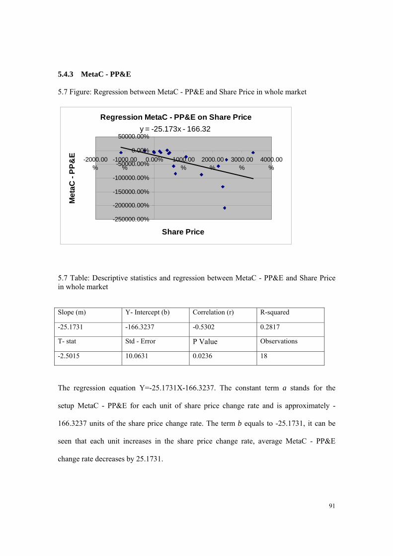
91

5.4.3 MetaC - PP&E

5.7 Figure: Regression between MetaC - PP&E and Share Price in whole market

Regression MetaC - PP&E on Share Price

y = -25.173x - 166.32

-250000.00%

-200000.00%

-150000.00%

-100000.00%

-50000.00%

0.00%

50000.00%

-2000.00%

-1000.00%

0.00% 1000.00%

2000.00%

3000.00%

4000.00%

Share Price

Me

taC

- P

P&

E

5.7 Table: Descriptive statistics and regression between MetaC - PP&E and Share Price in whole market

The regression equation Y=-25.1731X-166.3237. The constant term a stands for the

setup MetaC - PP&E for each unit of share price change rate and is approximately -

166.3237 units of the share price change rate. The term b equals to -25.1731, it can be

seen that each unit increases in the share price change rate, average MetaC - PP&E

change rate decreases by 25.1731.

Slope (m) Y- Intercept (b) Correlation (r) R-squared

-25.1731 -166.3237 -0.5302 0.2817

T- stat Std - Error P Value Observations

-2.5015 10.0631 0.0236 18

92

R2 =28.17% is moderately small. It tells us that 28.17% of the variation in percentage of

MetaC - PP&E change rate is explained by the independent variable share price.

Furthermore, it is implied that 71.83% of the variation in the percentage of MetaC -

PP&E change rate remains unexplained. Overall, the model provides a poor fit. P Value

0.0236 is smaller than 0.05, but the t-stat is -2.5015, so it is not accepted as statistically

significant.

Tests of Hypotheses

Hypotheses:

H0: μ =0 (there is no linear relationship) n=18

H1: μ ≠0 (there is a linear relationship) (two – tailed test)

Significance level: α = 0.05 tcrit =t α/2, n-1df=

t 0.025, 17df=2.110

Decision rule: Reject H0 if t calc >2.110 or if t calc < -2.110

Do not reject H0 if -2.110 ≤ t calc ≤ 2.110

Test statistic:

t= -2.5015

Conclusion: Since t calc < t critical (-2.5015 < -2.110) H0 was not rejected, it can be

concluded that there is sufficient evidence at the 5 % level of significance to suggest that

ˆ

ˆ

b

bt

s

93

share price change rate is negatively linearly related to the dependent variable, MetaC –

PP& E change rate.

5.4.4 MetaC – TA

5.8 Figure: Regression between MetaC – TA and Share Price in whole market

Regression of MetaC - TA on Share Price

y = 1.5479x + 60.568

-10000.00%

0.00%

10000.00%

20000.00%

30000.00%

40000.00%

50000.00%

-2000.00%

-1000.00%

0.00% 1000.00% 2000.00% 3000.00% 4000.00%

Share Price

Me

taC

- T

A

5.8 Table: Descriptive statistics and regression between MetaC – TA and Share Price in whole market

The regression equation Y=1.5479X+60.5675. R2 =2.78% is very small. It tells us that

2.78% of the variation in percentage of MetaC - TA change rate is explained by the

independent variable share price. Furthermore, it is implied that 97.22% of the variation

Slope (m) Y- Intercept (b) Correlation (r) R-squared

1.5479 60.5675 0.1666 0.0278

T- stat Std - Error P Value Observations

0.6758. 2.2905 0.5088 18

94

in the percentage of MetaC - TA change rate remains unexplained. Overall, the model

does not provide a good fit.

Share price b equals to 1.5479, this means that each unit increases in the share price

change rate, average MetaC - TA change rate increases by 1.5479. P Value 0.5088 is

much bigger than 0.05, so it is not accepted as statistically significant. The standard error

2.2905 measured the dispersion associated with the underlying population and the error

associated with the sampling process.

Tests of Hypotheses

Hypotheses:

H0: μ =0 (there is no linear relationship) n=18

H1: μ ≠0 (there is a linear relationship) (two – tailed test)

Significance level: α = 0.05 tcrit =t α/2, n-1df=

t 0.025, 17df=2.110

Decision rule: Reject H0 if t calc >2.110 or if t calc < -2.110

Do not reject H0 if -2.110 ≤ t calc ≤ 2.110

Test statistic:

t= 0.6758

ˆ

ˆ

b

bt

s

95

Conclusion: Since t calc < t critical (0.6758 < 2.110) H0 was not rejected, it can be concluded

that there is insufficient evidence at the 5 % level of significance to suggest that share

price change rate is linearly related to the dependent variable, MetaC - TA change rate.

5.4.5 MetaC - NWC/TA

5.9 Figure: Regression between MetaC - NWC/TA and Share Price in whole market

Regression of MetaC - NWC/TA on Share Price

y = -18.521x - 65.027

-350000.00%

-300000.00%

-250000.00%

-200000.00%

-150000.00%

-100000.00%

-50000.00%

0.00%

50000.00%

-2000.00%

-1000.00%

0.00% 1000.00%

2000.00%

3000.00%

4000.00%

Share Price

Me

taC

- N

WC

/TA

5.9 Table: Descriptive statistics and regression between MetaC - NWC/TA and Share Price in whole market

Slope (m) Y- Intercept (b) Correlation (r) R-squared

-18.5211 -65.0266 -0.2855 0.0815

T- stat Std - Error P Value Observations

-1.1917 15.5414 0.2507 18

96

The regression equation Y=-18.5211X–65.0266. The term b is huge negative number -

18.5211; this means that for each unit increase in the share price change rate, average

MetaC – NWC/TA change rate decreases by -18.5211.

R2 =8.15% is very small. It tells us that 8.15% of the variation in percentage of MetaC –

NWC/TA change rate is explained by the independent variable share price. Furthermore,

it is implied that 91.85% of the variation in the percentage of MetaC – NWC/TA change

rate remains unexplained. Overall, the model provides a poor fit.

P Value is also bigger number with 25.07% and it is much bigger than 0.05, so it is not

accepted as statistically significant. The standard error 15.5414 stands for the dispersion

associated with the underlying population and the error associated with the sampling

process.

Tests of Hypotheses

Hypotheses:

H0: μ =0 (there is no linear relationship) n=18

H1: μ ≠0 (there is a linear relationship) (two – tailed test)

Significance level: α = 0.05 tcrit =t α/2, n-1df=

t 0.025, 17df=2.110

Decision rule: Reject H0 if t calc >2.110 or if t calc < -2.110

Do not reject H0 if -2.110 ≤ t calc ≤ 2.110

97

Test statistic:

t= -1.1917

Conclusion: Since t critical ≤ t calc ≤ t critical (-2.110 <-1.1917 < 2.110) H0 was not rejected,

it can be concluded that there is insufficient evidence at the 5 % level of significance to

suggest that share price change rate is linearly related to the dependent variable, MetaC –

NWC/TA change rate.

5.4.6 MetaC - PP&E/TA

5.10 Figure: Regression between MetaC - PP&E/TA and Share Price in whole market

Regression of MetaC - PP&E/TA on Share Price

y = -67.691x + 3392.7

-500000.00%

0.00%

500000.00%

1000000.00%

1500000.00%

2000000.00%

2500000.00%

3000000.00%

-2000.00%

-1000.00%

0.00% 1000.00%

2000.00%

3000.00%

4000.00%

Share Price

Me

taC

- P

P&

E/T

A

ˆ

ˆ

b

bt

s

98

5.10 Table: Descriptive statistics and regression between MetaC - PP&E/TA and Share Price in whole market

The regression equation Y=-69.691X+3392.7441. The share price term b equals to -

67.691 and it is negative huge number, it can be seen that each unit increase in the share

price change rate, average MetaC – PP&E/TA change rate decreases by 69.691.The

constant term a represents the setup MetaC – PP&E/TA change rate for each unit of share

price change rate and is approximately 3392.7441 units of the share price change rate.

The standard error 147.1110 stands for the bigger error between the MetaC – PP&E/TA

change rate and the share price change rate. R2 =1.31% is very small. It tells us that

1.31% of the variation in percentage of MetaC – PP&E/TA change rate is explained by

the independent variable share price. Furthermore, it is implied that 98.69% of the

variation in the percentage of MetaC – PP&E/TA change rate remains unexplained.

Therefore, the model provides a poor fit.

Tests of Hypotheses

Hypotheses:

H0: μ =0 (there is no linear relationship) n=18

H1: μ ≠0 (there is a linear relationship) (two – tailed test)

Slope (m) Y- Intercept (b) Correlation (r) R-squared

-67.6909 3392.7441 -0.1143 0.0131

T- stat Std - Error P Value Observations

-0.4601 147.1110 0.6516 18

99

Significance level: α = 0.05 tcrit =t α/2, n-1df=

t 0.025, 17df=2.110

Decision rule: Reject H0 if t calc >2.110 or if t calc < -2.110

Do not reject H0 if -2.110 ≤ t calc ≤ 2.110

Test statistic:

t= -0.4601

Conclusion: Since t critical ≤ t calc ≤ t critical (-2.110 <-0.4601 < 2.110) H0 was not rejected,

it can be concluded that there is insufficient evidence at the 5 % level of significance to

suggest that share price change rate is linearly related to the dependent variable, MetaC

– PP&E/TA change rate.

ˆ

ˆ

b

bt

s

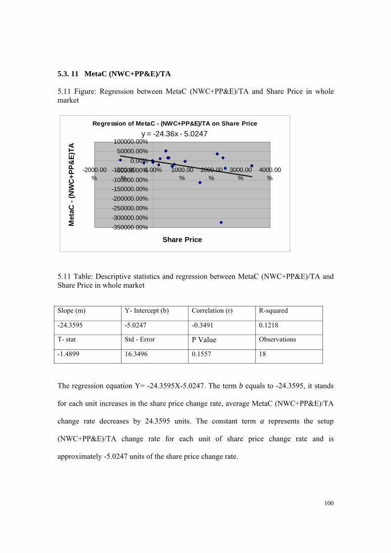
100

5.3. 11 MetaC (NWC+PP&E)/TA

5.11 Figure: Regression between MetaC (NWC+PP&E)/TA and Share Price in whole market

Regression of MetaC - (NWC+PP&E)/TA on Share Price

y = -24.36x - 5.0247

-350000.00%

-300000.00%

-250000.00%

-200000.00%

-150000.00%

-100000.00%

-50000.00%

0.00%

50000.00%

100000.00%

-2000.00%

-1000.00%

0.00% 1000.00%

2000.00%

3000.00%

4000.00%

Share Price

Met

aC -

(N

WC

+P

P&

E)T

A

5.11 Table: Descriptive statistics and regression between MetaC (NWC+PP&E)/TA and Share Price in whole market

The regression equation Y= -24.3595X-5.0247. The term b equals to -24.3595, it stands

for each unit increases in the share price change rate, average MetaC (NWC+PP&E)/TA

change rate decreases by 24.3595 units. The constant term a represents the setup

(NWC+PP&E)/TA change rate for each unit of share price change rate and is

approximately -5.0247 units of the share price change rate.

Slope (m) Y- Intercept (b) Correlation (r) R-squared

-24.3595 -5.0247 -0.3491 0.1218

T- stat Std - Error P Value Observations

-1.4899 16.3496 0.1557 18

101

R2 =12.18 % is moderately small. It tells us that 12.18% of the variation in percentage of

(NWC+PP&E)/TA change rate is explained by the independent variable share price.

Furthermore, it is implied that 87.82 of the variation in the percentage of

(NWC+PP&E)/TA change rate remains unexplained. Therefore, the model provides a

poor fit. P Value is the value ranges from zero to one. P Value 15.57% is more than 0.05,

so it is not accepted as statistically significant. The standard error 16.3496 is the bigger

errors between the (NWC & PP&E)/TA change rate and share price change rate.

Tests of Hypotheses

Hypotheses:

H0: μ =0 (there is no linear relationship) n=18

H1: μ ≠0 (there is a linear relationship) (two – tailed test)

Significance level: α = 0.05 tcrit =t α/2, n-1df=

t 0.025, 17df=2.110

Decision rule: Reject H0 if t calc >2.110 or if t calc < -2.110

Do not reject H0 if -2.110 ≤ t calc ≤ 2.110

Test statistic:

t= -1.4899

Conclusion: Since t critical ≤ t calc ≤ t critical (-2.110 <-1.4899 < 2.110) H0 was not rejected,

it can be concluded that there is insufficient evidence at the 5 % level of significance to

ˆ

ˆ

b

bt

s

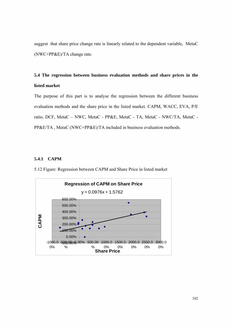
102

suggest that share price change rate is linearly related to the dependent variable, MetaC

(NWC+PP&E)/TA change rate.

5.4 The regression between business evaluation methods and share prices in the

listed market

The purpose of this part is to analyse the regression between the different business

evaluation methods and the share price in the listed market. CAPM, WACC, EVA, P/E

ratio, DCF, MetaC – NWC, MetaC - PP&E, MetaC - TA, MetaC - NWC/TA, MetaC -

PP&E/TA , MetaC (NWC+PP&E)/TA included in business evaluation methods.

5.4.1 CAPM

5.12 Figure: Regression between CAPM and Share Price in listed market

Regression of CAPM on Share Price

y = 0.0976x + 1.5762

-100.00%

0.00%

100.00%

200.00%

300.00%

400.00%

500.00%

600.00%

-1000.00%

-500.00%

0.00% 500.00%

1000.00%

1500.00%

2000.00%

2500.00%

3000.00%

Share Price

CA

PM

103

5.12 Table: Descriptive statistics and regression between CAPM and Share Price in listed market

The regression equation Y=0.0976X+1.5762. R2 =49.98% is moderately large. It tells us

that 49.98 % of the variation in percentage of CAPM change rate is explained by the

independent variable share price. On the other hand, it is implied that 50.02 % of the

variation in the percentage of CAPM change rate remains unexplained. Therefore, the

model provides a good fit.

The term b equals to 0.0976, it is clear that each unit increases in the share price change

rate, average CAPM change rate increases by 0.0976. The term a is equal to 1.5762.P

Value 0.00219 is less than 0.05 and t-stat 3.7266 is more than 1.96, so it is accepted as

statistically significant. The standard error 0.02619 has shown that there is not large

difference in error between CAPM change rate and the share price change rate.

Tests of Hypotheses

Hypotheses:

H0: μ =0 (there is no linear relationship) n=16

H1: μ ≠0 (there is a linear relationship) (two – tailed test)

Significance level: α = 0.05 tcrit =t α/2, n-1df=

Slope (m) Y- Intercept (b) Correlation (r) R-squared

0.0976 1.5762 0.7069 0.4998

T- stat Std - Error P Value Observations

3.7266 0.02619 0.00219 16

104

t 0.025, 15df=2.131

Decision rule: Reject H0 if t calc >2.131 or if t calc < -2.131

Do not reject H0 if -2.131 ≤ t calc ≤ 2.131

Test statistic:

t= 3.7266

Conclusion: Since t calc > t critical (3.7266> 2.131) H0 was rejected, it can be concluded that

there is sufficient sample evidence at the 5 % level of significance to suggest that there is

a stronger linear relationship between share price change rate and CAPM change rate.

5.4.2 WACC

5.13 Figure: Regression between WACC and Share Price in listed market

Regression of WACC on Share Price

y = 0.0839x + 1.3491

0.00%

100.00%

200.00%

300.00%

400.00%

500.00%

600.00%

-1000.00%

-500.00%

0.00% 500.00%

1000.00%

1500.00%

2000.00%

2500.00%

3000.00%

Share Price

WA

CC

ˆ

ˆ

b

bt

s

105

5.13 Table: Descriptive statistics and regression between WACC and Share Price in listed market

The regression equation Y=0.0839X+1.3491. P Value 0.0104 is less than 0.05, and T-

stat 3.1482 is much more than 1.96 so it is accepted as statistically significant. The

standard error 0.02665 balances the dispersion associated with the underlying population

and the error associated with the sampling process.

Share price b equals to 0.0839. This means that each unit increases in the share price

change rate, average WACC change rate increases by 0.0839 units. The constant term a

stands for the setup WACC for each unit of share price change rate and is approximately

1.3491 units of the share price change rate.

R2 =49.74% is moderately large. It tells us that 49.74 % of the variation in percentage of

WACC change rate is explained by the independent variable share price change rate.

Furthermore, it is implied that 50.26% of the variation in the percentage of WACC

change rate remains unexplained. Therefore, the model provides a good fit.

Tests of Hypotheses

Hypotheses:

Slope (m) Y- Intercept (b) Correlation (r) R-squared

0.0839 1.3491 0.7053 0.4974

T- stat Std - Error P Value Observations

3.1482 0.02665 0.0104 12

106

H0: μ =0 (there is no linear relationship) n=12

H1: μ ≠0 (there is a linear relationship) (two – tailed test)

Significance level: α = 0.05 tcrit =t α/2, n-1df=

t 0.025, 11df=2.201

Decision rule: Reject H0 if t calc >2.201 or if t calc < -2.201

Do not reject H0 if -2.201 ≤ t calc ≤ 2.201

Test statistic:

t= 3.1482

Conclusion: Since t calc > t critical (3.1482 > 2.201) H0 was rejected, it can be concluded

that there is sufficient sample evidence at the 5 % level of significance to suggest that

there is a stronger linear relationship between share price change rate and WACC

change rate.

ˆ

ˆ

b

bt

s

107

5.4.3 EVA

5.14 Figure: Regression between EVA and Share Price in listed market

Regression of EVA on Share Price

y = 0.0057x + 0.1749

-50.00%

0.00%

50.00%

100.00%

150.00%

-1000.00%

-500.00%

0.00% 500.00%

1000.00%

1500.00%

2000.00%

2500.00%

3000.00%

Share Price

EV

A

5.14 Table: Descriptive statistics and regression between EVA and Share Price in listed market

The regression equation Y=0.00567X+0.1749. The term b equals to 0.00567, it is clear

that each unit increase in the share price change rate, average EVA change rate increases

by 0.00567.

R2 =1.53% is very small. It can be seen that 1.53 % of the variation in percentage of EVA

change rate is explained by the independent variable share price. Furthermore, it means

Slope (m) Y- Intercept (b) Correlation (r) R-squared

0.00567 0.1749 0.1235 0.0153

T- stat Std - Error P Value Observations

0.3730 0.0152 0.7174 11

108

that 98.47 of the variation in the percentage of EVA change rate remain unexplained.

Therefore, the model does not provide a good fit.

P Value with 0.7174 is much more than 0.05, so it is not accepted as statistically

significant. The standard error 0.0152 represents the dispersion associated with the

underlying population and the error associated with the sampling process.

Tests of Hypotheses

Hypotheses:

H0: μ =0 (there is no linear relationship) n=11

H1: μ ≠0 (there is a linear relationship) (two – tailed test)

Significance level: α = 0.05 t crit =t α/2, n-1df=

t 0.025, 10df=2.228

Decision rule: Reject H0 if t calc >2.228 or if t calc < -2.228

Do not reject H0 if -2.228 ≤ t calc ≤ 2.228

Test statistic:

t= 0.3730

Conclusion: Since t calc < t critical (0.3730 < 2.228) H0 was not rejected, it can be

concluded that there is insufficient evidence at the 5 % level of significance to suggest

ˆ

ˆ

b

bt

s

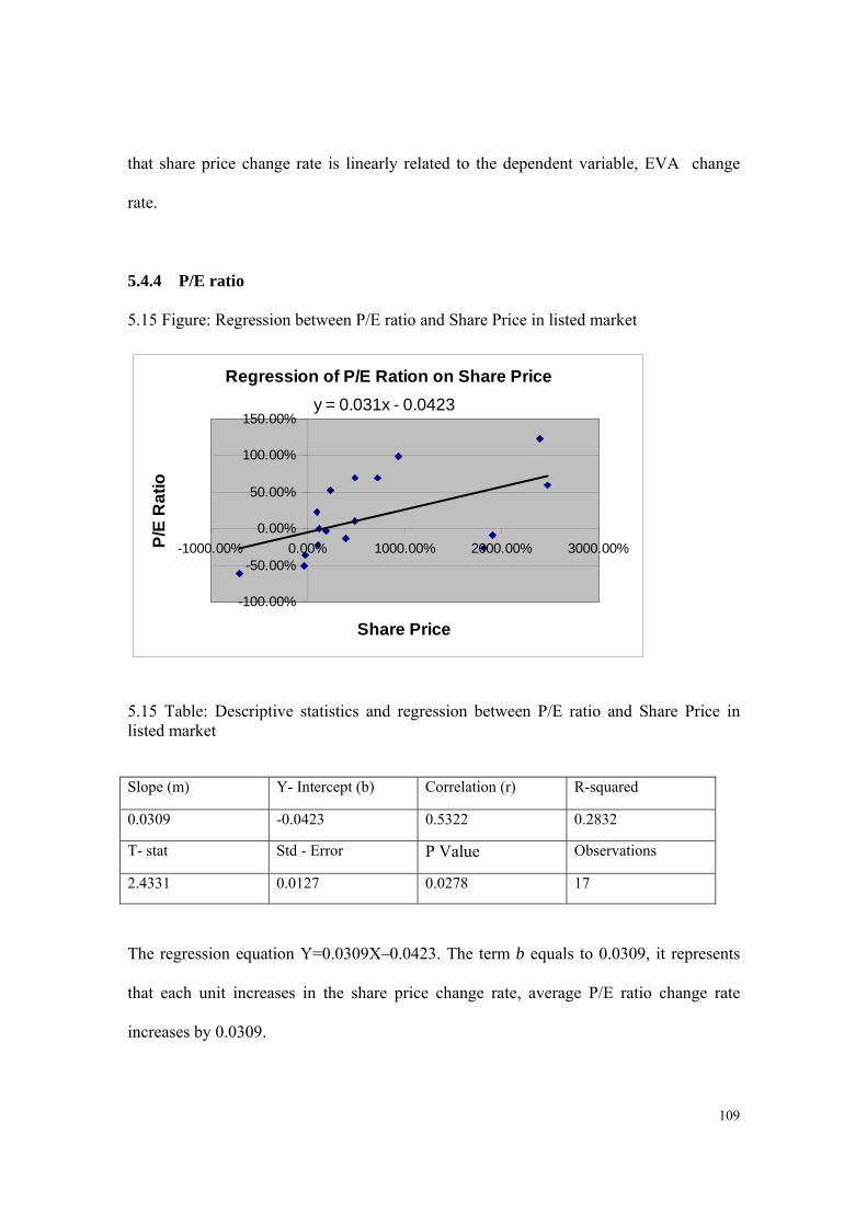
109

that share price change rate is linearly related to the dependent variable, EVA change

rate.

5.4.4 P/E ratio

5.15 Figure: Regression between P/E ratio and Share Price in listed market

5.15 Table: Descriptive statistics and regression between P/E ratio and Share Price in listed market

The regression equation Y=0.0309X–0.0423. The term b equals to 0.0309, it represents

that each unit increases in the share price change rate, average P/E ratio change rate

increases by 0.0309.

Slope (m) Y- Intercept (b) Correlation (r) R-squared

0.0309 -0.0423 0.5322 0.2832

T- stat Std - Error P Value Observations

2.4331 0.0127 0.0278 17

Regression of P/E Ration on Share Price

y = 0.031x - 0.0423

-100.00%

-50.00%

0.00%

50.00%

100.00%

150.00%

-1000.00% 0.00% 1000.00% 2000.00% 3000.00%

Share Price

P/E

Ra

tio

110

P Value 0.0278 is much less than 0.05 and T-stat 2.4331 much more than 1.96, so it is

accepted as statistically significant. R2 =28.32%, moderately medium, It tells us that

28.32 % of the variation in percentage of P/E ratio change rate is explained by the

independent variable share price.

In addition, it is implied that 71.68% of the variation in the percentage of P/E ratio

change rate remains unexplained. Overall, the model provides a poor fit. The standard

error 0.0127 stands for the existing error between the P/E ratio change rate and the share

price change rate.

Tests of Hypotheses

Hypotheses:

H0: μ =0 (there is no linear relationship) n=17

H1: μ ≠0 (there is a linear relationship) (two – tailed test)

Significance level: α = 0.05 tcrit =t α/2, n-1df=

t 0.025, 16df=2.120

Decision rule: Reject H0 if t calc >2.120 or if t calc < -2.120

Do not reject H0 if -2.120 ≤ t calc ≤ 2.120

Test statistic:

t= 2.4331

ˆ

ˆ

b

bt

s

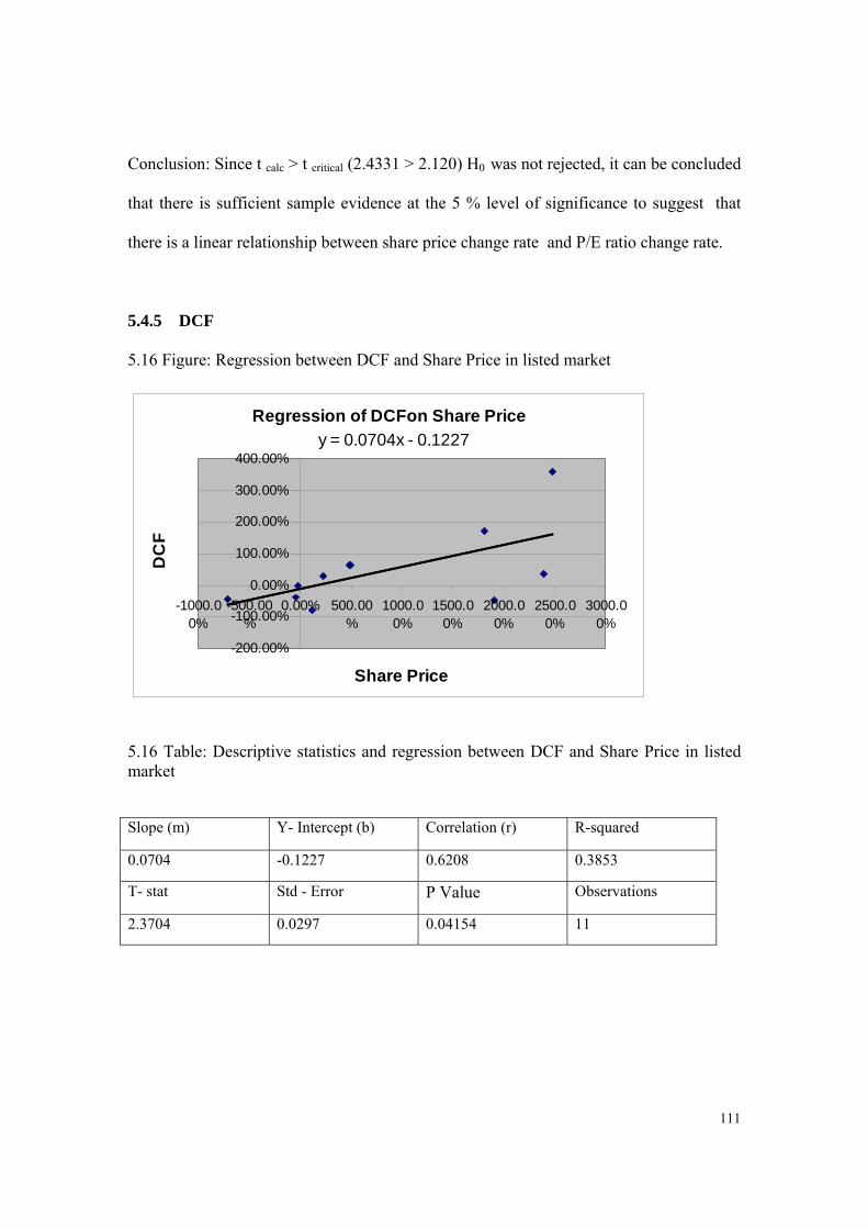
111

Conclusion: Since t calc > t critical (2.4331 > 2.120) H0 was not rejected, it can be concluded

that there is sufficient sample evidence at the 5 % level of significance to suggest that

there is a linear relationship between share price change rate and P/E ratio change rate.

5.4.5 DCF

5.16 Figure: Regression between DCF and Share Price in listed market

Regression of DCFon Share Price

y = 0.0704x - 0.1227

-200.00%

-100.00%

0.00%

100.00%

200.00%

300.00%

400.00%

-1000.00%

-500.00%

0.00% 500.00%

1000.00%

1500.00%

2000.00%

2500.00%

3000.00%

Share Price

DC

F

5.16 Table: Descriptive statistics and regression between DCF and Share Price in listed market

Slope (m) Y- Intercept (b) Correlation (r) R-squared

0.0704 -0.1227 0.6208 0.3853

T- stat Std - Error P Value Observations

2.3704 0.0297 0.04154 11

112

The regression equation Y=0.0704X–0.1227. R2 =38.53 % is moderately medium. It is

clear that 38.53 % of the variation in percentage of DCF change rate is explained by the

independent variable share price. On the other hand, it is implied that 61.47% of the

variation in the percentage of DCF change rate remains unexplained. Overall, the model

provides a better fit.

P Value 0.04154 is less than 0.05 and T-stat is 2.3704, it has shown that it is accepted as

statistically significant. The standard error 0.0297 represents the dispersion associated

with the underlying population and the error associated with the sampling process.

Share price term b equals to 0.0704; this means that each unit increases in the share price

change rate, average DCF change rate increases by 0.0704.

Tests of Hypotheses

Hypotheses:

H0: μ =0 (there is no linear relationship) n=11

H1: μ ≠0 (there is a linear relationship) (two – tailed test)

Significance level: α = 0.05 tcrit =t α/2, n-1df=

t 0.025, 10df=2.228

Decision rule: Reject H0 if t calc >2.228 or if t calc < -2.228

Do not reject H0 if -2.228 ≤ t calc ≤ 2.228

Test statistic: ˆ

ˆ

b

bt

s

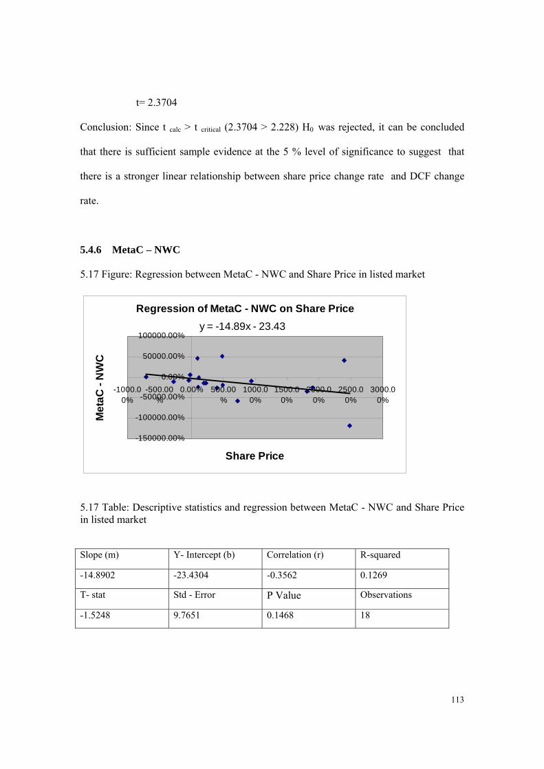
113

t= 2.3704

Conclusion: Since t calc > t critical (2.3704 > 2.228) H0 was rejected, it can be concluded

that there is sufficient sample evidence at the 5 % level of significance to suggest that

there is a stronger linear relationship between share price change rate and DCF change

rate.

5.4.6 MetaC – NWC

5.17 Figure: Regression between MetaC - NWC and Share Price in listed market

Regression of MetaC - NWC on Share Price

y = -14.89x - 23.43

-150000.00%

-100000.00%

-50000.00%

0.00%

50000.00%

100000.00%

-1000.00%

-500.00%

0.00% 500.00%

1000.00%

1500.00%

2000.00%

2500.00%

3000.00%

Share Price

Me

taC

- N

WC

5.17 Table: Descriptive statistics and regression between MetaC - NWC and Share Price in listed market

Slope (m) Y- Intercept (b) Correlation (r) R-squared

-14.8902 -23.4304 -0.3562 0.1269

T- stat Std - Error P Value Observations

-1.5248 9.7651 0.1468 18

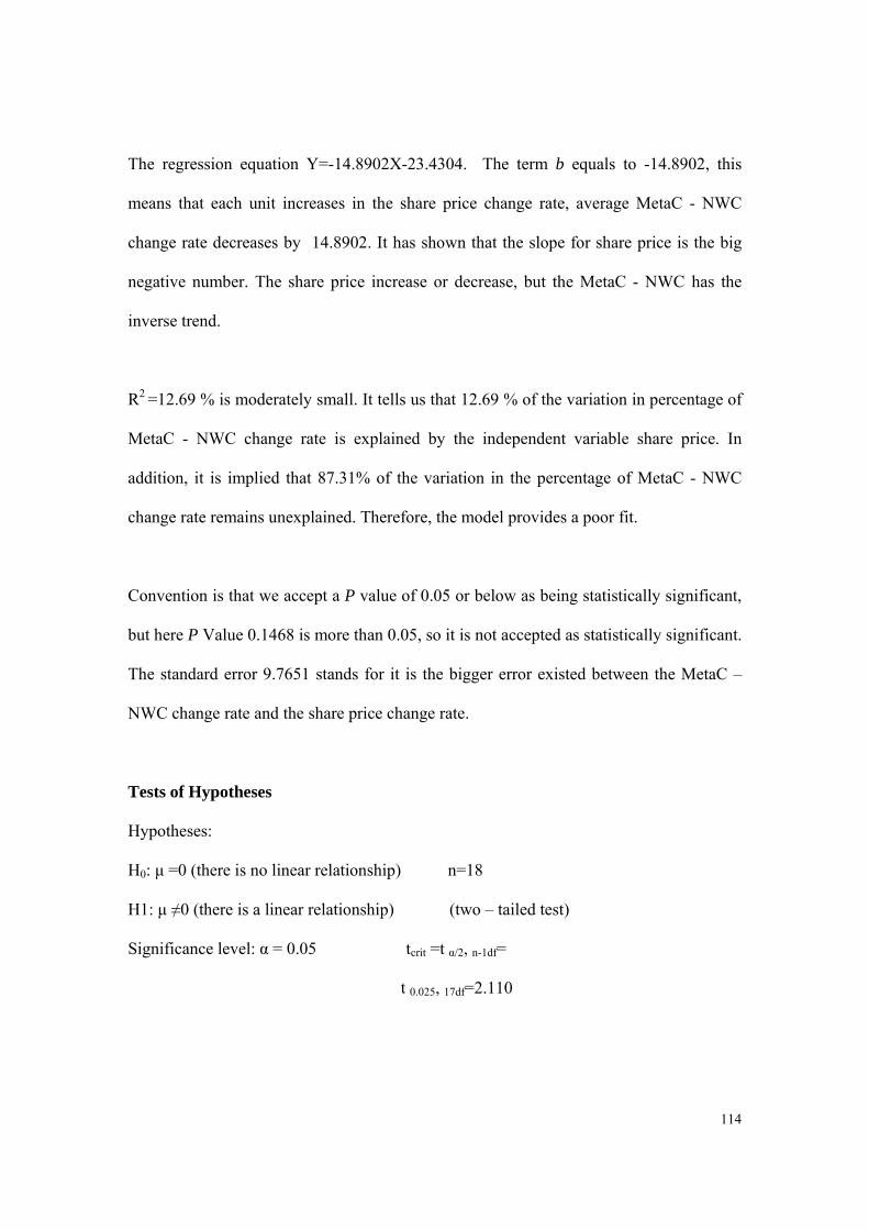
114

The regression equation Y=-14.8902X-23.4304. The term b equals to -14.8902, this

means that each unit increases in the share price change rate, average MetaC - NWC

change rate decreases by 14.8902. It has shown that the slope for share price is the big

negative number. The share price increase or decrease, but the MetaC - NWC has the

inverse trend.

R2 =12.69 % is moderately small. It tells us that 12.69 % of the variation in percentage of

MetaC - NWC change rate is explained by the independent variable share price. In

addition, it is implied that 87.31% of the variation in the percentage of MetaC - NWC

change rate remains unexplained. Therefore, the model provides a poor fit.

Convention is that we accept a P value of 0.05 or below as being statistically significant,

but here P Value 0.1468 is more than 0.05, so it is not accepted as statistically significant.

The standard error 9.7651 stands for it is the bigger error existed between the MetaC –

NWC change rate and the share price change rate.

Tests of Hypotheses

Hypotheses:

H0: μ =0 (there is no linear relationship) n=18

H1: μ ≠0 (there is a linear relationship) (two – tailed test)

Significance level: α = 0.05 tcrit =t α/2, n-1df=

t 0.025, 17df=2.110

115

Decision rule: Reject H0 if t calc >2.110 or if t calc < -2.110

Do not reject H0 if -2.110 ≤ t calc ≤ 2.110

Test statistic:

t= -1.5248

Conclusion: Since t critical ≤ t calc ≤ t critical (-2.110 < -1.5248 < 2.110) H0 was not rejected,

it can be concluded that there is insufficient evidence at the 5 % level of significance to

suggest that share price change rate is linearly related to the dependent variable, MetaC –

NWC change rate.

5.4.7 MetaC - PP&E

5.18 Figure: Regression between MetaC - PP&E and Share Price in listed market

Regression of MetaC- PP&E on Share Price

y = -15.468x - 311.27

-250000.00%

-200000.00%

-150000.00%

-100000.00%

-50000.00%

0.00%

50000.00%

-1000.00% 0.00% 1000.00% 2000.00% 3000.00%

Share Price

Me

taC

- P

P&

E

ˆ

ˆ

b

bt

s

116

5.18 Table: Descriptive statistics and regression between MetaC - PP&E and Share Price in listed market

The regression equation Y=-15.4678X -311.2695. The MetaC - PP&E term b of 15.4678

is the bigger slope for the share price, it means that each unit increases in the share price

change rate, average MetaC - PP&E change rate decreases by -15.4678. And the MetaC -

PP&E term b has the bigger inverse relationship with the share price change rate.

R2 =6.39 % is very small. It tells us that 6.39 % of the variation in percentage of MetaC -

PP&E change rate is explained by the independent variable share price. Furthermore, it is

implied that 6.39 % of the variation in the percentage of MetaC - PP&E change rate

remains unexplained. Therefore, the model provides a poor fit.

Generally, P value stands for the probability of observing a test statistic that is as extreme

as or more extreme than currently observed assuming that the null hypothesis is true. P

Value 0.3115 is more than 0.05, so it is not accepted as statistically significant. The

standard error 14.7987 represents the bigger error that existing between MetaC - PP&E

change rate and the share price change rate.

Tests of Hypotheses

Slope (m) Y- Intercept (b) Correlation (r) R-squared

-15.4678 -311.2695 -0.2528 0.0639

T- stat Std - Error P Value Observations

-1.0452 14.7987 0.3115 18

117

Hypotheses:

H0: μ =0 (there is no linear relationship) n=18

H1: μ ≠0 (there is a linear relationship) (two – tailed test)

Significance level: α = 0.05 tcrit =t α/2, n-1df=

t 0.025, 17df=2.110

Decision rule: Reject H0 if t calc >2.110 or if t calc < -2.110

Do not reject H0 if -2.110 ≤ t calc ≤ 2.110

Test statistic:

t= -1.0452

Conclusion: Since t critical ≤ t calc ≤ t critical (-2.110 < -1.0452 < 2.110) H0 was not rejected,

it can be concluded that there is insufficient evidence at the 5 % level of significance to

suggest that share price change rate is linearly related to the dependent variable, MetaC –

PP&E change rate.

ˆ

ˆ

b

bt

s

118

5.4.8 MetaC – TA

5.19 Figure: Regression between MetaC – TA and Share Price in listed market

Regression of MetaC - TA on Share Price

y = 2.3806x + 48.272

-10000.00%

0.00%

10000.00%

20000.00%

30000.00%

40000.00%

-1000.00%

-500.00%

0.00% 500.00%

1000.00%

1500.00%

2000.00%

2500.00%

3000.00%

Share Price

Me

taC

- T

A

5.19 Table: Descriptive statistics and regression between MetaC – TA and Share Price in listed market

The regression equation Y=2.3806X+48.2719. The constant term a 48.2719 represents

the setup MetaC – TA for each unit of share price change rate and is approximately 48.27

units of the share price change rate. And the term b equals to 2.3806, it can be explained

that each unit increase in the share price change rate, average MetaC – TA change rate

increases by 2.3806.

Slope (m) Y- Intercept (b) Correlation (r) R-squared

2.3806 48.2719 0.2012 0.04047

T- stat Std - Error P Value Observations

0.8216 2.8974 0.4234 18

119

R2 =4.047% is very small. It tells us that 4.047% of the variation in percentage of MetaC

– TA change rate is explained by the independent variable share price. Furthermore, it is

implied that 95.953% of the variation in the percentage of MetaC – TA change rate

remains unexplained. It is clear that the model provides a poor fit.

Commonly, we accepted the P value of 0.05 or below as being statistically significant. P

Value 0.4234 is much more than 0.05, so it is not accepted as statistically significant. The

standard error 2.8974 stands for the dispersion associated with the underlying population

and the error associated with the sampling process.

Tests of Hypotheses

Hypotheses:

H0: μ =0 (there is no linear relationship) n=18

H1: μ ≠0 (there is a linear relationship) (two – tailed test)

Significance level: α = 0.05 tcrit =t α/2, n-1df=

t 0.025, 17df=2.110

Decision rule: Reject H0 if t calc >2.110 or if t calc < -2.110

Do not reject H0 if -2.110 ≤ t calc ≤ 2.110

Test statistic:

t= 0.8216

ˆ

ˆ

b

bt

s

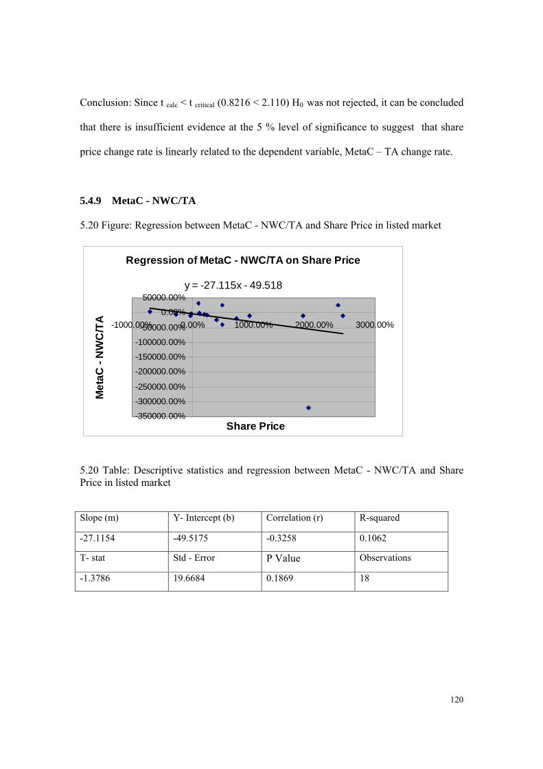
120

Conclusion: Since t calc < t critical (0.8216 < 2.110) H0 was not rejected, it can be concluded

that there is insufficient evidence at the 5 % level of significance to suggest that share

price change rate is linearly related to the dependent variable, MetaC – TA change rate.

5.4.9 MetaC - NWC/TA

5.20 Figure: Regression between MetaC - NWC/TA and Share Price in listed market

Regression of MetaC - NWC/TA on Share Price

y = -27.115x - 49.518

-350000.00%

-300000.00%

-250000.00%

-200000.00%

-150000.00%

-100000.00%

-50000.00%

0.00%

50000.00%

-1000.00% 0.00% 1000.00% 2000.00% 3000.00%

Share Price

Me

taC

- N

WC

/TA

5.20 Table: Descriptive statistics and regression between MetaC - NWC/TA and Share Price in listed market

Slope (m) Y- Intercept (b) Correlation (r) R-squared

-27.1154 -49.5175 -0.3258 0.1062

T- stat Std - Error P Value Observations

-1.3786 19.6684 0.1869 18

121

The regression equation Y=-27.1154X-49.5175. Share price term b equals to -27.1154,

this is the bigger slope and it represents for each unit increase in the share price change

rate, average MetaC - NWC/TA change rate decrease by -27.1154.

R2 =10.62% is moderately small. It seems likely that that 10.62 % of the variation in

percentage of MetaC - NWC/TA change rate is explained by the independent variable

share price. Furthermore, it explains that 89.38% of the variation in the percentage of

MetaC - NWC/TA change rate remains unexplained. Therefore, the model provides a

poor fit. P Value is the probability of observing a test statistic that is as extreme as or

more extreme than currently observed assuming that the null hypothesis is true. P Value

0.1869 is more than 0.05, so it is not accepted as statistically significant.

Tests of Hypotheses

Hypotheses:

H0: μ =0 (there is no linear relationship) n=18

H1: μ ≠0 (there is a linear relationship) (two – tailed test)

Significance level: α = 0.05 tcrit =t α/2, n-1df=

t 0.025, 17df=2.110

Decision rule: Reject H0 if t calc >2.110 or if t calc < -2.110

Do not reject H0 if -2.110 ≤ t calc ≤ 2.110

Test statistic:

ˆ

ˆ

b

bt

s

122

t= -1.3786

Conclusion: Since t critical ≤ t calc ≤ t critical (-2.110 <-1.3786 < 2.110) H0 was not rejected, it

can be concluded that there is insufficient evidence at the 5 % level of significance to

suggest that share price change rate is linearly related to the dependent variable, MetaC –

NWC/TA change rate.

5.4.10 MetaC - PP&E/TA

5.21 Figure: Regression between MetaC - PP&E/TA and Share Price in listed market

Regression of MetaC - PP&E/TA on Share Price

y = -72.247x + 3168.9

0.00%

500000.00%

1000000.00%

1500000.00%

2000000.00%

2500000.00%

3000000.00%

-1000.00% 0.00% 1000.00% 2000.00% 3000.00%

Share Price

Me

taC

- P

P&

E/T

A

5.21 Table: Descriptive statistics and regression between MetaC - PP&E/TA and Share Price in listed market

Slope (m) Y- Intercept (b) Correlation (r) R-squared

-72.2466 3168.8629 -0.09608 0.00923

T- stat Std - Error P Value Observations

-0.3861 187.1189 0.7045 18

123

The regression equation Y=-72.2466X+3168.8629. It can be seen that there is a larger

figure for the constant term a of 3168.8629. Where the term b equals to -72.2466; this

means that each unit increases in the share price change rate, average MetaC - PP&E/TA

change rate decreases by -72.2466 units.

R2 =0.923 %. It seems like 0.923 % of the variation in percentage of MetaC - PP&E/TA

change rate is explained by the independent variable share price. Furthermore, it is

implied that 99.077 % of the variation in the percentage of MetaC - PP&E/TA change

rate remains unexplained. P Value 0.7045 is much more than 0.05, so it is not accepted

as statistically significant. On the other hand, there are very bigger standard error of

187.11 between the share price change rate and the MetaC - PP&E/TA change rate.

Tests of Hypotheses

Hypotheses:

H0: μ =0 (there is no linear relationship) n=18

H1: μ ≠0 (there is a linear relationship) (two – tailed test)

Significance level: α = 0.05 tcrit =t α/2, n-1df=

t 0.025, 17df=2.110

Decision rule: Reject H0 if t calc >2.110 or if t calc < -2.110

Do not reject H0 if -2.110 ≤ t calc ≤ 2.110

Test statistic:

ˆ

ˆ

b

bt

s

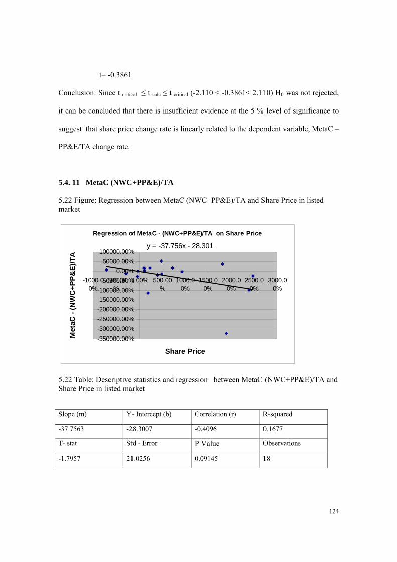
124

t= -0.3861

Conclusion: Since t critical ≤ t calc ≤ t critical (-2.110 < -0.3861< 2.110) H0 was not rejected,

it can be concluded that there is insufficient evidence at the 5 % level of significance to

suggest that share price change rate is linearly related to the dependent variable, MetaC –

PP&E/TA change rate.

5.4. 11 MetaC (NWC+PP&E)/TA

5.22 Figure: Regression between MetaC (NWC+PP&E)/TA and Share Price in listed market

Regression of MetaC - (NWC+PP&E)/TA on Share Price

y = -37.756x - 28.301

-350000.00%

-300000.00%

-250000.00%

-200000.00%

-150000.00%

-100000.00%

-50000.00%

0.00%

50000.00%

100000.00%

-1000.00%

-500.00%

0.00% 500.00%

1000.00%

1500.00%

2000.00%

2500.00%

3000.00%

Share Price

Met

aC -

(N

WC

+P

P&

E)/

TA

5.22 Table: Descriptive statistics and regression between MetaC (NWC+PP&E)/TA and Share Price in listed market

Slope (m) Y- Intercept (b) Correlation (r) R-squared

-37.7563 -28.3007 -0.4096 0.1677

T- stat Std - Error P Value Observations

-1.7957 21.0256 0.09145 18

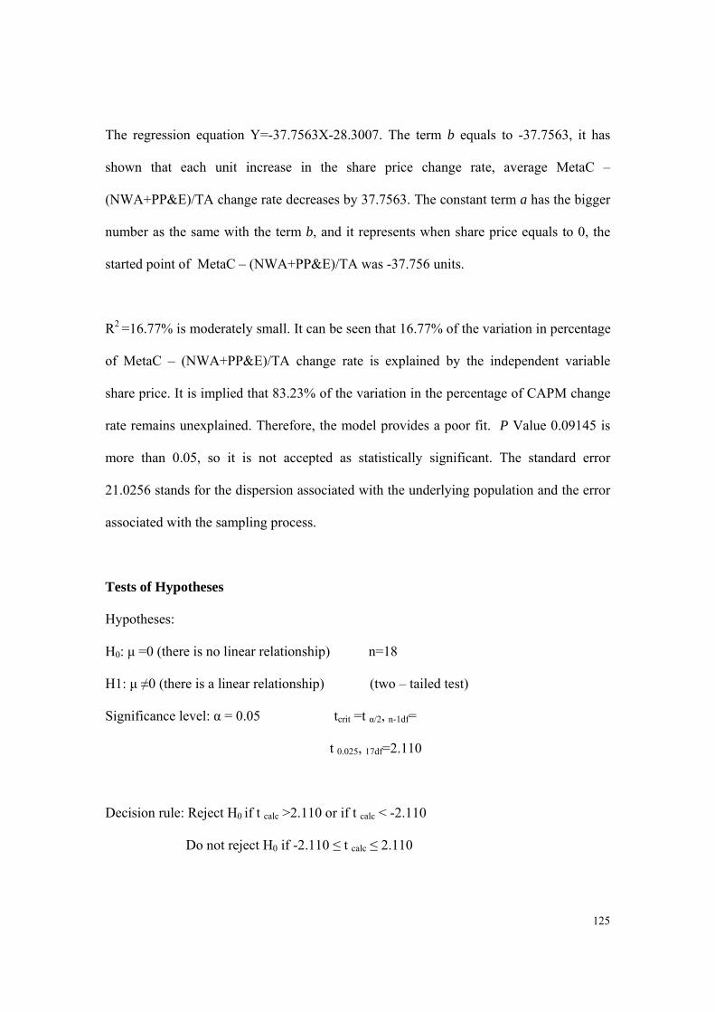
125

The regression equation Y=-37.7563X-28.3007. The term b equals to -37.7563, it has

shown that each unit increase in the share price change rate, average MetaC –

(NWA+PP&E)/TA change rate decreases by 37.7563. The constant term a has the bigger

number as the same with the term b, and it represents when share price equals to 0, the

started point of MetaC – (NWA+PP&E)/TA was -37.756 units.

R2 =16.77% is moderately small. It can be seen that 16.77% of the variation in percentage

of MetaC – (NWA+PP&E)/TA change rate is explained by the independent variable

share price. It is implied that 83.23% of the variation in the percentage of CAPM change

rate remains unexplained. Therefore, the model provides a poor fit. P Value 0.09145 is

more than 0.05, so it is not accepted as statistically significant. The standard error

21.0256 stands for the dispersion associated with the underlying population and the error

associated with the sampling process.

Tests of Hypotheses

Hypotheses:

H0: μ =0 (there is no linear relationship) n=18

H1: μ ≠0 (there is a linear relationship) (two – tailed test)

Significance level: α = 0.05 tcrit =t α/2, n-1df=

t 0.025, 17df=2.110

Decision rule: Reject H0 if t calc >2.110 or if t calc < -2.110

Do not reject H0 if -2.110 ≤ t calc ≤ 2.110

126

Test statistic:

t= -1.7957

Conclusion: Since t critical ≤ t calc ≤ t critical (-2.110 < -1.7957< 2.110) H0 was not rejected,

it can be concluded that there is insufficient evidence at the 5 % level of significance to

suggest that share price change rate is linearly related to the dependent variable, MetaC –

(NWA+PP&E)/TA change rate.

5.5 The regression between business evaluation methods and share prices in the

delisted market

The purpose of this part is to analyse the regression between the different business

evaluation methods and the share price in the delisted market. CAPM, WACC, EVA, P/E

ratio, DCF, MetaC – NWC, MetaC - PP&E, MetaC - TA, MetaC - NWC/TA, MetaC -

PP&E/TA , MetaC (NWC+PP&E)/TA included in business evaluation methods.

ˆ

ˆ

b

bt

s

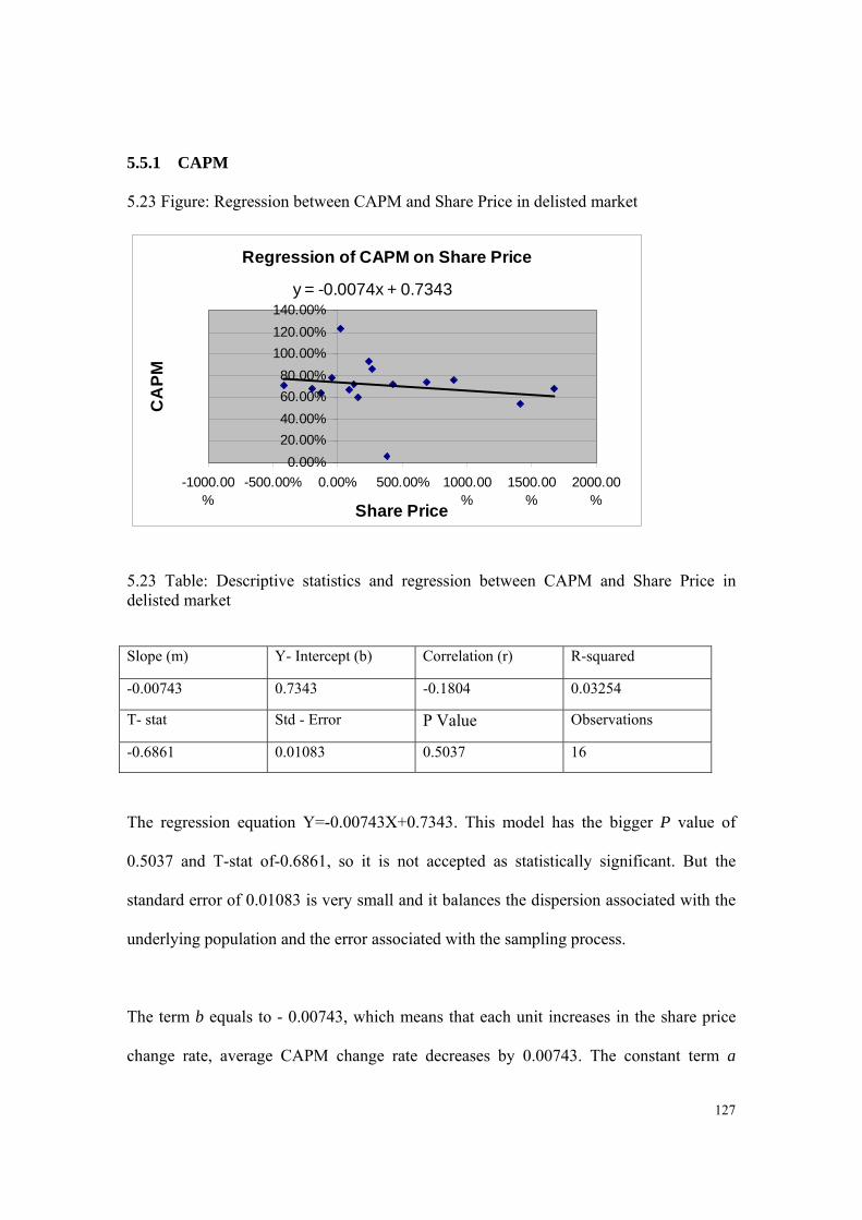
127

5.5.1 CAPM

5.23 Figure: Regression between CAPM and Share Price in delisted market

Regression of CAPM on Share Price

y = -0.0074x + 0.7343

0.00%

20.00%

40.00%

60.00%

80.00%

100.00%

120.00%

140.00%

-1000.00%

-500.00% 0.00% 500.00% 1000.00%

1500.00%

2000.00%

Share Price

CA

PM

5.23 Table: Descriptive statistics and regression between CAPM and Share Price in delisted market

The regression equation Y=-0.00743X+0.7343. This model has the bigger P value of

0.5037 and T-stat of-0.6861, so it is not accepted as statistically significant. But the

standard error of 0.01083 is very small and it balances the dispersion associated with the

underlying population and the error associated with the sampling process.

The term b equals to - 0.00743, which means that each unit increases in the share price

change rate, average CAPM change rate decreases by 0.00743. The constant term a

Slope (m) Y- Intercept (b) Correlation (r) R-squared

-0.00743 0.7343 -0.1804 0.03254

T- stat Std - Error P Value Observations

-0.6861 0.01083 0.5037 16

128

represents the setup CAPM for each unit of share price change rate and is approximately

0.7343 units of the share price change rate.

R2 =3.25% is very small. It has shown that 3.25 % of the variation in percentage of

CAPM change rate is explained by the independent variable share price. Furthermore, it

is implied that 3.25 % of the variation in the percentage of CAPM change rate remains

unexplained. Therefore, the model provides a poor fit.

Tests of Hypotheses

Hypotheses:

H0: μ =0 (there is no linear relationship) n=16

H1: μ ≠0 (there is a linear relationship) (two – tailed test)

Significance level: α = 0.05 t crit =t α/2, n-1df=

t 0.025, 15df=2.131

Decision rule: Reject H0 if t calc >2.131or if t calc < -2.131

Do not reject H0 if -2.131≤ t calc ≤ 2.131

Test statistic:

t= -0.6861

ˆ

ˆ

b

bt

s

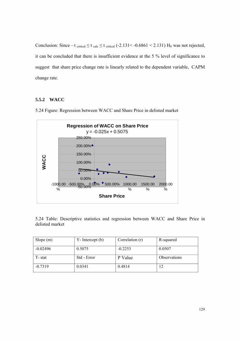
129

Conclusion: Since – t critical ≤ t calc ≤ t critical (-2.131< -0.6861 < 2.131) H0 was not rejected,

it can be concluded that there is insufficient evidence at the 5 % level of significance to

suggest that share price change rate is linearly related to the dependent variable, CAPM

change rate.

5.5.2 WACC

5.24 Figure: Regression between WACC and Share Price in delisted market

Regression of WACC on Share Pricey = -0.025x + 0.5075

-50.00%

0.00%

50.00%

100.00%

150.00%

200.00%

250.00%

-1000.00%

-500.00% 0.00% 500.00% 1000.00%

1500.00%

2000.00%

Share Price

WA

CC

5.24 Table: Descriptive statistics and regression between WACC and Share Price in delisted market

Slope (m) Y- Intercept (b) Correlation (r) R-squared

-0.02496 0.5075 -0.2253 0.0507

T- stat Std - Error P Value Observations

-0.7319 0.0341 0.4814 12

130

The regression equation Y=-0.02496X+0.5075. R2 =5.07 % is very small. It can be seen

that 5.07 % of the variation in percentage of WACC change rate is explained by the

independent variable share price.

Furthermore, it is implied that 94.93 % of the variation in the percentage of WACC

change rate remains unexplained. Therefore, the model provides a poor fit. P Value

0.4814 is much larger than 0.05, so it is not accepted as statistically significant. The

standard error 0.0341 stands for the smaller error between the share price changer rate

and the WACC change rate.

Share price term b equals to 0.5075, it means that each unit increases in the share price

change rate, average WACC change rate increases by 0.5075 units. The constant term a

represents the setup CAPM for each unit of share price change rate and is approximately

0.5 units of the share price change rate.

Tests of Hypotheses

Hypotheses:

H0: μ =0 (there is no linear relationship) n=12

H1: μ ≠0 (there is a linear relationship) (two – tailed test)

Significance level: α = 0.05 tcrit =t α/2, n-1df=

t 0.025, 11df=2.201

Decision rule: Reject H0 if t calc >2.201or if t calc < -2.201

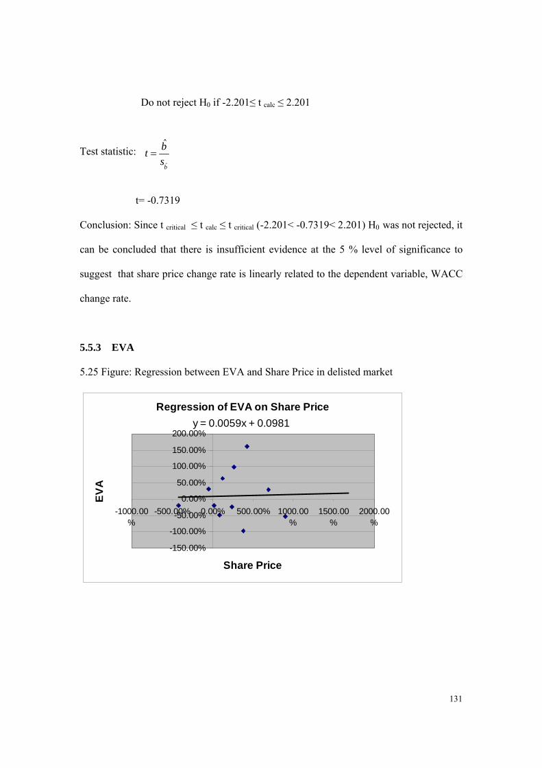
131

Do not reject H0 if -2.201≤ t calc ≤ 2.201

Test statistic:

t= -0.7319

Conclusion: Since t critical ≤ t calc ≤ t critical (-2.201< -0.7319< 2.201) H0 was not rejected, it

can be concluded that there is insufficient evidence at the 5 % level of significance to

suggest that share price change rate is linearly related to the dependent variable, WACC

change rate.

5.5.3 EVA

5.25 Figure: Regression between EVA and Share Price in delisted market

Regression of EVA on Share Price

y = 0.0059x + 0.0981

-150.00%

-100.00%

-50.00%

0.00%

50.00%

100.00%

150.00%

200.00%

-1000.00%

-500.00% 0.00% 500.00% 1000.00%

1500.00%

2000.00%

Share Price

EV

A

ˆ

ˆ

b

bt

s

132

5.25 Table: Descriptive statistics and regression between EVA and Share Price in delisted market

The regression equation Y=0.00587X+0.098112. The term b equals to 0.00587, it seems

likely that each unit increases in the share price change rate, with the average EVA

change rate increases by 0.00587. The term a represents when x (share price) equals to 0,

the started point of EVA was 0.098112 percentages.

R2 =0.079%, it represents 0.079 % of the variation in percentage of EVA change rate is

explained by the independent variable share price. On the other hand, it is implied that

99.921% of the variation in the percentage of EVA change rate remains unexplained.

Therefore, the model was not able to explain a correlation between the share price and the

EVA.

P is the probability of observing a test statistic that is as extreme as or more extreme than

currently observed assuming that the null hypothesis is true. P Value 0.9346 is much

more than 0.05, so it is not accepted as statistically significant. The standard error of

0.06956 represents the errors between the predicted value and true value.

Tests of Hypotheses

Slope (m) Y- Intercept (b) Correlation (r) R-squared

0.00587 0.098112 0.02813 0.00079

T- stat Std - Error P Value Observations

0.0844 0.06956 0.9346 11

133

Hypotheses:

H0: μ =0 (there is no linear relationship) n=11

H1: μ ≠0 (there is a linear relationship) (two – tailed test)

Significance level: α = 0.05 tcrit =t α/2, n-1df=

t 0.025, 10df=2.228

Decision rule: Reject H0 if t calc >2.228or if t calc < -2.228

Do not reject H0 if -2.228 ≤ t calc ≤ 2.228

Test statistic:

t= 0.0844

Conclusion: Since t calc < t critical 0.0844< 2.201 H0 was not rejected, it can be concluded

that there is insufficient evidence at the 5 % level of significance to suggest that share

price change rate is linearly related to the dependent variable, EVA change rate.

ˆ

ˆ

b

bt

s

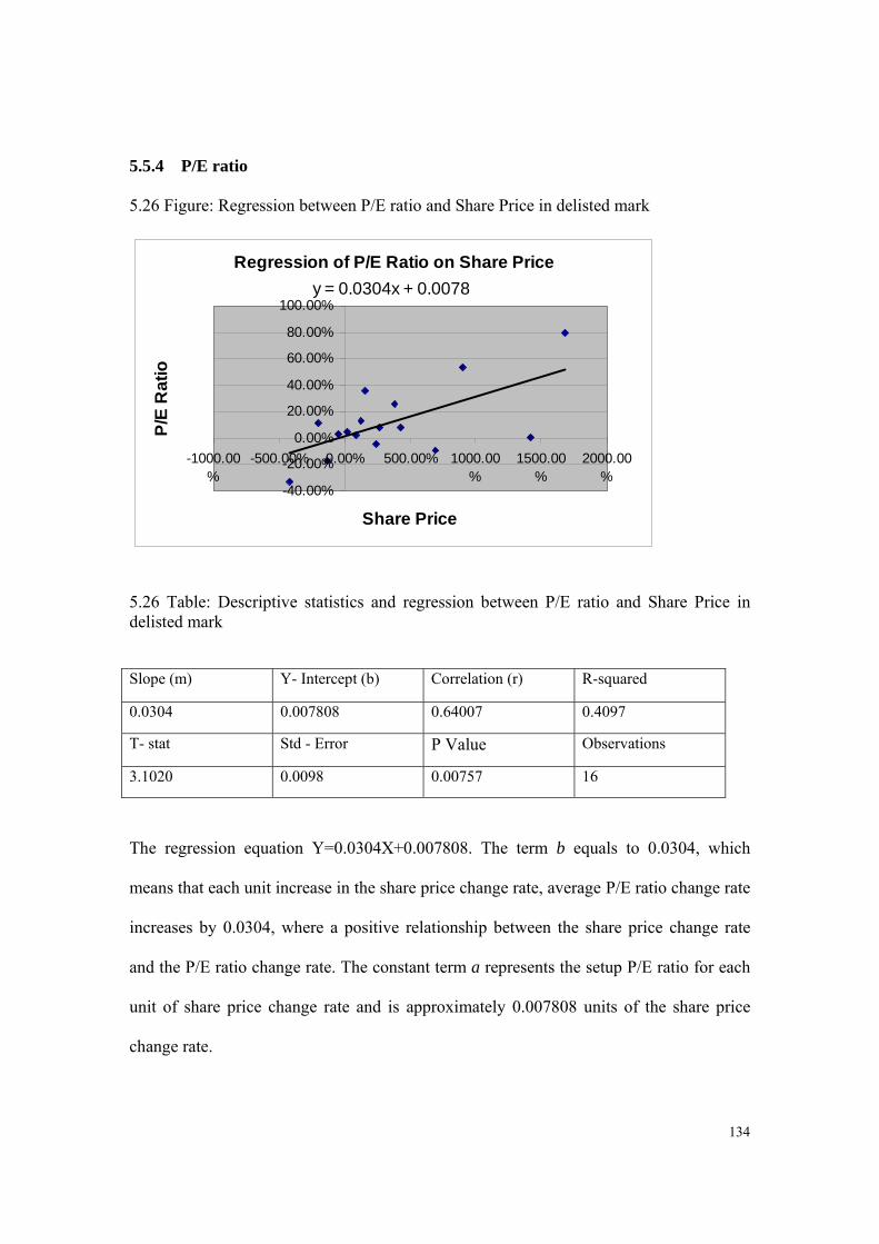
134

5.5.4 P/E ratio

5.26 Figure: Regression between P/E ratio and Share Price in delisted mark

Regression of P/E Ratio on Share Price

y = 0.0304x + 0.0078

-40.00%

-20.00%

0.00%

20.00%

40.00%

60.00%

80.00%

100.00%

-1000.00%

-500.00% 0.00% 500.00% 1000.00%

1500.00%

2000.00%

Share Price

P/E

Ra

tio

5.26 Table: Descriptive statistics and regression between P/E ratio and Share Price in delisted mark

The regression equation Y=0.0304X+0.007808. The term b equals to 0.0304, which

means that each unit increase in the share price change rate, average P/E ratio change rate

increases by 0.0304, where a positive relationship between the share price change rate

and the P/E ratio change rate. The constant term a represents the setup P/E ratio for each

unit of share price change rate and is approximately 0.007808 units of the share price

change rate.

Slope (m) Y- Intercept (b) Correlation (r) R-squared

0.0304 0.007808 0.64007 0.4097

T- stat Std - Error P Value Observations

3.1020 0.0098 0.00757 16

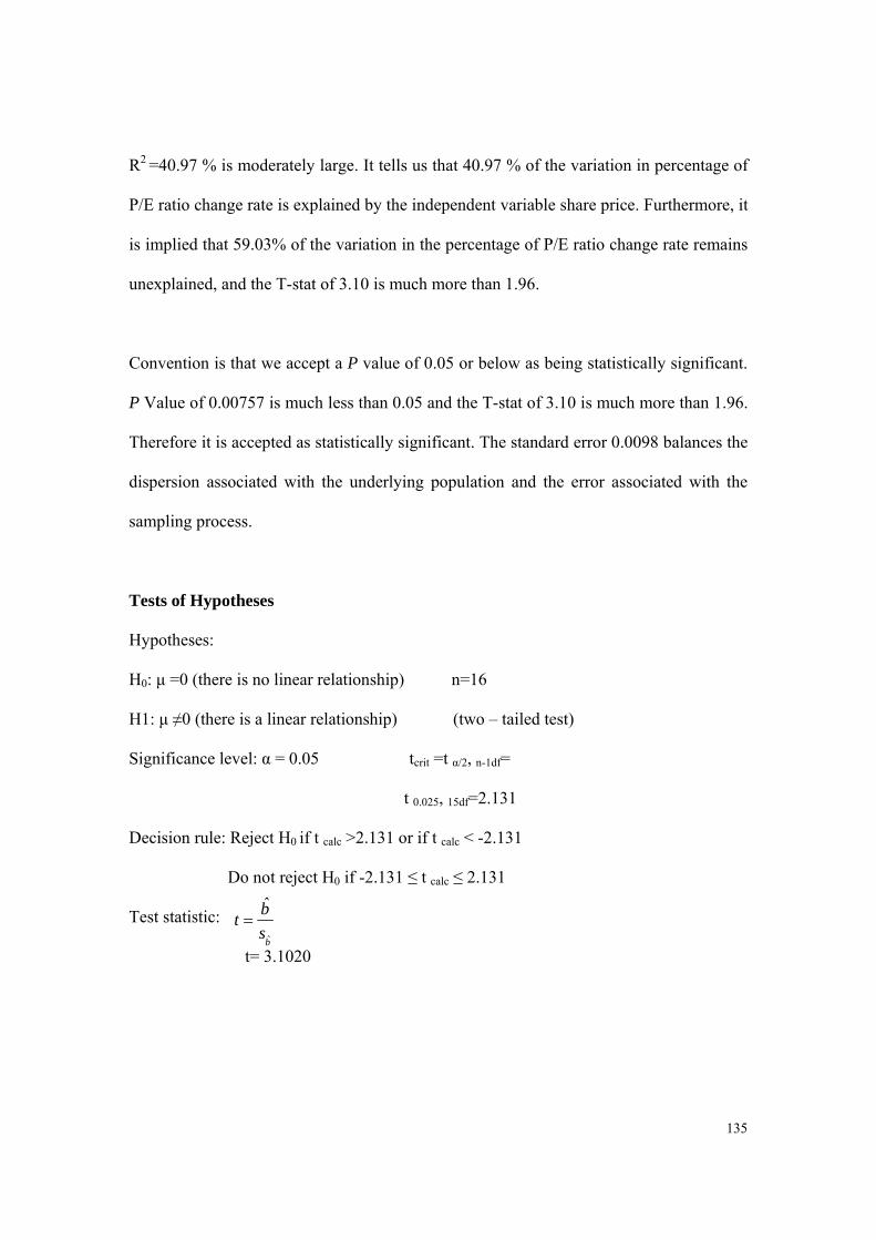
135

R2 =40.97 % is moderately large. It tells us that 40.97 % of the variation in percentage of

P/E ratio change rate is explained by the independent variable share price. Furthermore, it

is implied that 59.03% of the variation in the percentage of P/E ratio change rate remains

unexplained, and the T-stat of 3.10 is much more than 1.96.

Convention is that we accept a P value of 0.05 or below as being statistically significant.

P Value of 0.00757 is much less than 0.05 and the T-stat of 3.10 is much more than 1.96.

Therefore it is accepted as statistically significant. The standard error 0.0098 balances the

dispersion associated with the underlying population and the error associated with the

sampling process.

Tests of Hypotheses

Hypotheses:

H0: μ =0 (there is no linear relationship) n=16

H1: μ ≠0 (there is a linear relationship) (two – tailed test)

Significance level: α = 0.05 tcrit =t α/2, n-1df=

t 0.025, 15df=2.131

Decision rule: Reject H0 if t calc >2.131 or if t calc < -2.131

Do not reject H0 if -2.131 ≤ t calc ≤ 2.131

Test statistic:

t= 3.1020 ˆ

ˆ

b

bt

s

136

Conclusion: Since t calc > t critical (3.1020> 2.131) H0 was rejected, it can be concluded that

there is sufficient sample evidence at the 5 % level of significance to suggest that there is

a stronger linear relationship between share price change rate and P/E ratio change rate.

5.5.5 DCF

5.27 Figure: Regression between DCF and Share Price in delisted market

Regression of DCF on Share Price

y = 0.7171x - 3.1677

-1500.00%

-1000.00%

-500.00%

0.00%

500.00%

1000.00%

-1000.00%

-500.00% 0.00% 500.00% 1000.00%

1500.00%

2000.00%

Share Price

DC

F

5.27 Table: Descriptive statistics and regression between DCF and Share Price in delisted market

The regression equation Y=0.7171X–3.1677. P Value of 0.0432 is less than 0.05, and the

T-stat of 2.3991 is more than 1.96, so it is accepted as statistically significant. The

Slope (m) Y- Intercept (b) Correlation (r) R-squared

0.7171 -3.1677 0.6469 0.4184

T- stat Std - Error P Value Observations

2.3991 0.2989 0.0432 10

137

standard error 0.2989 embodies dispersion between the underlying population and the

error associated with the sampling process.

R2 =41.84 % is moderately large. The results indicate that 41.84 % of the variation in

percentage of DCF change rate is explained by the independent variable share price.

Furthermore, it tells us 58.16 % of the variation in the percentage of DCF change rate

remains unexplained.

The term b equals to 0.7171; it stands for each unit increases in the share price change

rate, average DCF change rate increases by 0.7171.The constant term a represents the

setup DCF for each unit of share price change rate and is approximately -3.1677 units of

the share price change rate.

Tests of Hypotheses

Hypotheses:

H0: μ =0 (there is no linear relationship) n=10

H1: μ ≠0 (there is a linear relationship) (two – tailed test)

Significance level: α = 0.05 tcrit =t α/2, n-1df=

t 0.025, 9df=2.262

Decision rule: Reject H0 if t calc >2.262or if t calc < -2.262

Do not reject H0 if -2.262≤ t calc ≤ 2.262

Test statistic:

ˆ

ˆ

b

bt

s

138

t= 2.3991

Conclusion: Since t calc > t critical (2.3991> 2.262) H0 was rejected, it can be concluded that

there is sufficient sample evidence at the 5 % level of significance to suggest that there is

a linear relationship between share price change rate and DCF change rate.

5.5.6 MetaC – NWC

5.28 Figure: Regression between MetaC – NWC and Share Price in delisted market

Regression of MetaC - NWC on Share Price

y = 2.592x - 35.998

-30000.00%

-25000.00%

-20000.00%

-15000.00%

-10000.00%

-5000.00%

0.00%

5000.00%

10000.00%

-1000.00%

-500.00% 0.00% 500.00% 1000.00%

1500.00%

2000.00%

Share Price

Me

taC

- N

WC

5.28 Table: Descriptive statistics and regression between MetaC – NWC and Share Price in delisted market

Slope (m) Y- Intercept (b) Correlation (r) R-squared

2.5920 -35.9983 0.2121 0.0449

T- stat Std - Error P Value Observations

0.8683 2.9853 0.3981 18

139

The regression equation Y=2.5920X-35.9983. The constant term a -35.9983 represents

when share price is equal to 0, the started point of MetaC – NWC was -35.9983. The term

b equals to 0.0446, it stands for each unit increase in the share price change rate, average

MetaC – NWC change rate increases by 2.5920.

R2 =4.49 % is very small. The results indicate that 4.49 % of the variation in percentage

of MetaC – NWC change rate is explained by the independent variable share price. The

results further indicate that 95.51 % of the variation in the percentage of MetaC – NWC

change rate remains unexplained. Therefore, the model provides a poor fit.

Generally, we accept a P value of 0.05 or below as being statistically significant. P Value

of 0.3981 is significantly more than 0.05, so it is not accepted as statistically significant.

The standard error 2.9853 explains the dispersion between the underlying population and

the error associated with the sampling process.

Tests of Hypotheses

Hypotheses:

H0: μ =0 (there is no linear relationship) n =18

H1: μ ≠0 (there is a linear relationship) (two – tailed test)

Significance level: α = 0.05 tcrit =t α/2, n-1df=

t 0.025, 17df=2.110

Decision rule: Reject H0 if t calc >2.110 or if t calc < -2.110

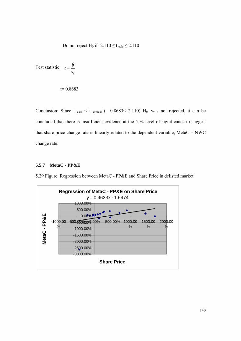
140

Do not reject H0 if -2.110 ≤ t calc ≤ 2.110

Test statistic:

t= 0.8683

Conclusion: Since t calc < t critical ( 0.8683< 2.110) H0 was not rejected, it can be

concluded that there is insufficient evidence at the 5 % level of significance to suggest

that share price change rate is linearly related to the dependent variable, MetaC – NWC

change rate.

5.5.7 MetaC - PP&E

5.29 Figure: Regression between MetaC - PP&E and Share Price in delisted market

Regression of MetaC - PP&E on Share Pricey = 0.4633x - 1.6474

-3000.00%

-2500.00%

-2000.00%

-1500.00%

-1000.00%

-500.00%

0.00%

500.00%

1000.00%

-1000.00%

-500.00% 0.00% 500.00% 1000.00%

1500.00%

2000.00%

Share Price

Me

taC

- P

P&

E

ˆ

ˆ

b

bt

s

141

5.29 Table: Descriptive statistics and regression between MetaC - PP&E and Share Price in delisted market

The regression equation Y=0.4633X–1.6474. The term b equals to 0.4633, and represents

each unit increase in the share price change rate, with an average MetaC - PP&E change

rate increase by 0.4633. The constant term a represents the setup MetaC - PP&E for each

unit of share price change rate and is approximately -1.65 units of the share price change

rate.

R2 =13.81% is moderately small. It seems as though 13.81 % with a variation in

percentage of MetaC - PP&E change rate is explained by the independent variable share

price. Furthermore, it is implied that 86.19 % of the variation in the percentage of MetaC

- PP&E change rate remains unexplained. Therefore, the model provided a poor fit.

The standard error 0.2988 stands for the errors between the underlying population and

the error associated with the sampling process. The accepted level of the P value of 0.05

or less is statistically significant. P Value 0.1419 is more than 0.05, so it is not accepted

as statistically significant.

Tests of Hypotheses

Slope (m) Y- Intercept (b) Correlation (r) R-squared

0.4633 -1.6474 0.3716 0.1381

T- stat Std - Error P Value Observations

1.5505 0.2988 0.1419 17

142

Hypotheses:

H0: μ =0 (there is no linear relationship) n=17

H1: μ ≠0 (there is a linear relationship) (two – tailed test)

Significance level: α = 0.05 tcrit =t α/2, n-1df=

t 0.025, 16df=2.120

Decision rule: Reject H0 if t calc >2.120 or if t calc < -2.120

Do not reject H0 if -2.120 ≤ t calc ≤ 2.120

Test statistic:

t= 1.5505

Conclusion: Since t calc < t critical ( 1.5505< 2.120) H0 was not rejected, it can be

concluded that there is insufficient evidence at the 5 % level of significance to suggest

that share price change rate is linearly related to the dependent variable, MetaC – PP&E

change rate.

ˆ

ˆ

b

bt

s

143

5.5.8 MetaC – TA

5.30 Figure: Regression between MetaC – TA and Share Price in delisted market

Regression of MetaC - TA on Share Price

y = 1.1149x + 8.4934

-5000.00%

0.00%

5000.00%

10000.00%

15000.00%

20000.00%

-1000.00%

-500.00% 0.00% 500.00% 1000.00%

1500.00%

2000.00%

Share Price

Me

taC

- T

A

5.30 Table: Descriptive statistics and regression between MetaC – TA and Share Price in delisted market

The regression equation Y=1.1149X+8.4934. R-squared equals to 2.1%, it tells us that

2.1% of the variation in percentage of MetaC - TA change rate is explained by the

independent variable share price. Furthermore, it is implied that 97.9% of the variation in

the percentage of CAPM change rate remains unexplained. Overall, the model provides a

poor fit.

Slope (m) Y- Intercept (b) Correlation (r) R-squared

1.1149 8.4934 0.1449 0.021

T- stat Std - Error P Value Observations

0.5859 1.9029 0.5661 18

144

P Value 0.5661 is more than 0.05, so it is not accept statistically significant generally,

the accepted the level is 0.05. The standard error represents that there are 1.9029 errors

existed between the share price change rate and the MetaC - TA change.

Share price b equals to 1.1149; it seems likely that each unit increases in the share price

change rate, average MetaC - TA change rate increases by 1.1149. The constant term a

represents the setup MetaC - TA for each unit of share price change rate and is

approximately 8.4934 units of the share price change rate.

Tests of Hypotheses

Hypotheses:

H0: μ =0 (there is no linear relationship) n=18

H1: μ ≠0 (there is a linear relationship) (two – tailed test)

Significance level: α = 0.05 t crit =t α/2, n-1df=

t 0.025, 17df=2.110

Decision rule: Reject H0 if t calc >2.110 or if t calc < -2.110

Do not reject H0 if -2.110 ≤ t calc ≤ 2.110

Test statistic:

t= 0.5859

Conclusion: Since t calc < t critical ( 0.5859 < 2.110) H0 was not rejected, it can be

concluded that there is insufficient evidence at the 5 % level of significance to suggest

ˆ

ˆ

b

bt

s

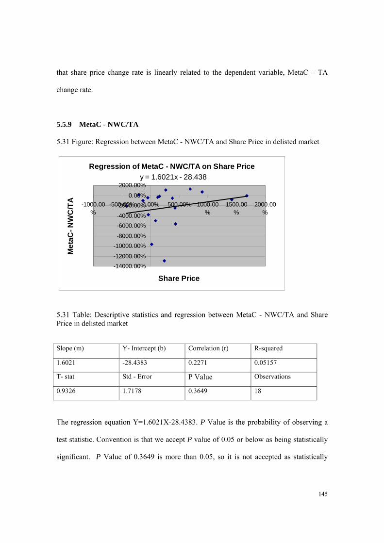
145

that share price change rate is linearly related to the dependent variable, MetaC – TA

change rate.

5.5.9 MetaC - NWC/TA

5.31 Figure: Regression between MetaC - NWC/TA and Share Price in delisted market

Regression of MetaC - NWC/TA on Share Price

y = 1.6021x - 28.438

-14000.00%

-12000.00%

-10000.00%

-8000.00%

-6000.00%

-4000.00%

-2000.00%

0.00%

2000.00%

-1000.00%

-500.00% 0.00% 500.00% 1000.00%

1500.00%

2000.00%

Share Price

Me

taC

- N

WC

/TA

5.31 Table: Descriptive statistics and regression between MetaC - NWC/TA and Share Price in delisted market

The regression equation Y=1.6021X-28.4383. P Value is the probability of observing a

test statistic. Convention is that we accept P value of 0.05 or below as being statistically

significant. P Value of 0.3649 is more than 0.05, so it is not accepted as statistically

Slope (m) Y- Intercept (b) Correlation (r) R-squared

1.6021 -28.4383 0.2271 0.05157

T- stat Std - Error P Value Observations

0.9326 1.7178 0.3649 18

146

significant. The standard error of 1.7178 represents the relationship between the

underlying population and the error associated with the sampling process.

R2 of 5.157 % tells us that 5.157 % of the variation in percentage of MetaC –NWC/TA

change rate is explained by the independent variable share price. And, it is implied that

94.943 % of the variation in the percentage of CAPM change rate remains unexplained.

Overall, the model provides a poor fit.

Where share price term b equals to 1.6021 each unit increases in the share price change

rate, average MetaC –NWC/TA change rate increases by 1.6021. The constant term a of -

28.43 represents that when x (share price) is equal to 0, the started points of MetaC –

NWC/TA is 2.51 units.

Tests of Hypotheses

Hypotheses:

H0: μ =0 (there is no linear relationship) n=18

H1: μ ≠0 (there is a linear relationship) (two – tailed test)

Significance level: α = 0.05 t crit =t α/2, n-1df=

t 0.025, 17df=2.110

Decision rule: Reject H0 if t calc >2.110 or if t calc < -2.110

Do not reject H0 if -2.110 ≤ t calc ≤ 2.110

Test statistic:

ˆ

ˆ

b

bt

s

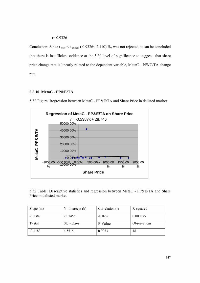
147

t= 0.9326

Conclusion: Since t calc < t critical ( 0.9326< 2.110) H0 was not rejected, it can be concluded

that there is insufficient evidence at the 5 % level of significance to suggest that share

price change rate is linearly related to the dependent variable, MetaC – NWC/TA change

rate.

5.5.10 MetaC - PP&E/TA

5.32 Figure: Regression between MetaC - PP&E/TA and Share Price in delisted market

Regression of MetaC - PP&E/TA on Share Price

y = -0.5387x + 28.746

-10000.00%

0.00%

10000.00%

20000.00%

30000.00%

40000.00%

50000.00%

-1000.00%

-500.00% 0.00% 500.00% 1000.00%

1500.00%

2000.00%

Share Price

Me

taC

- P

P&

E/T

A

5.32 Table: Descriptive statistics and regression between MetaC - PP&E/TA and Share Price in delisted market

Slope (m) Y- Intercept (b) Correlation (r) R-squared

-0.5387 28.7456 -0.0296 0.000875

T- stat Std - Error P Value Observations

-0.1183 4.5515 0.9073 18

148

The regression equation Y=-0.5387X+28.7456. The term b equals to -0.5387; it stands

for each unit increase in the share price change rate, average MetaC – PP&E/TA change

rate decreases by 0.5387. The a of appropriate 28.75 represents that when x (share price)

equals to 0, the started point of MetaC – PP&E/TA change rate was 2.51 percentage.

R2 of 0.0875 % tells us 0.0875 % of the variation in MetaC – PP&E/TA change rate is

explained by the independent variable share price. Furthermore, it is implied that nearly

100 % of the variation in the percentage of MetaC – PP&E/TA change rate remains

unexplained. Overall, the model is totally useless. P Value of 90.73% is far much more

than the 0.05, this means that there exists 100% probability to say that neither hypothesis

is true.

Tests of Hypotheses

Hypotheses:

H0: μ =0 (there is no linear relationship) n=18

H1: μ ≠0 (there is a linear relationship) (two – tailed test)

Significance level: α = 0.05 tcrit =t α/2, n-1df=

t 0.025, 17df=2.110

Decision rule: Reject H0 if t calc >2.110 or if t calc < -2.110

Do not reject H0 if -2.110 ≤ t calc ≤ 2.110

Test statistic: ˆ

ˆ

b

bt

s

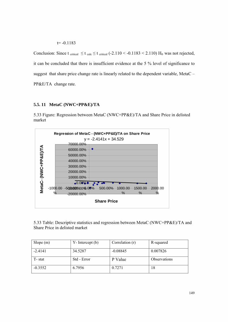
149

t= -0.1183

Conclusion: Since t critical ≤ t calc ≤ t critical (-2.110 < -0.1183 < 2.110) H0 was not rejected,

it can be concluded that there is insufficient evidence at the 5 % level of significance to

suggest that share price change rate is linearly related to the dependent variable, MetaC –

PP&E/TA change rate.

5.5. 11 MetaC (NWC+PP&E)/TA

5.33 Figure: Regression between MetaC (NWC+PP&E)/TA and Share Price in delisted market

Regression of MetaC - (NWC+PP&E)/TA on Share Price

y = -2.4141x + 34.529

-20000.00%

-10000.00%

0.00%

10000.00%

20000.00%

30000.00%

40000.00%

50000.00%

60000.00%

70000.00%

-1000.00%

-500.00% 0.00% 500.00% 1000.00%

1500.00%

2000.00%

Share Price

Met

aC-

(NW

C+

PP

&E

)/T

A

5.33 Table: Descriptive statistics and regression between MetaC (NWC+PP&E)/TA and Share Price in delisted market

Slope (m) Y- Intercept (b) Correlation (r) R-squared

-2.4141 34.5287 -0.08845 0.007826

T- stat Std - Error P Value Observations

-0.3552 6.7956 0.7271 18

150

The regression equation Y=-2.4141X+34.5287. The term b equals to -2.4141; it is seems

that each unit increases in the share price change rate, average MetaC –

(NWC+PP&E)/TA change rate decreases by 2.4141. The constant term a represents the

setup MetaC – (NWC+PP&E)/TA for each unit of share price change rate and is

approximately 34.5 units of the share price change rate.

R2 of 0.7826 % stands for only 0.7826 % of the variation in percentage of MetaC –

(NWC+PP&E)/TA change rate is explained by the independent variable share price.

Furthermore, it is implied that nearly 100 % of the variation in the percentage of MetaC –

(NWC+PP&E)/TA change rate remains unexplained. Overall, the model proves nothing.

P Value with 72.71 % has shown that it is much more than 0.05 and identified that this

model has no practice value.

Tests of Hypotheses

Hypotheses:

H0: μ =0 (there is no linear relationship) n=18

H1: μ ≠0 (there is a linear relationship) (two – tailed test)

Significance level: α = 0.05 tcrit =t α/2, n-1df=

t 0.025, 17df=2.110

Decision rule: Reject H0 if t calc >2.110 or if t calc < -2.110

Do not reject H0 if -2.110 ≤ t calc ≤ 2.110

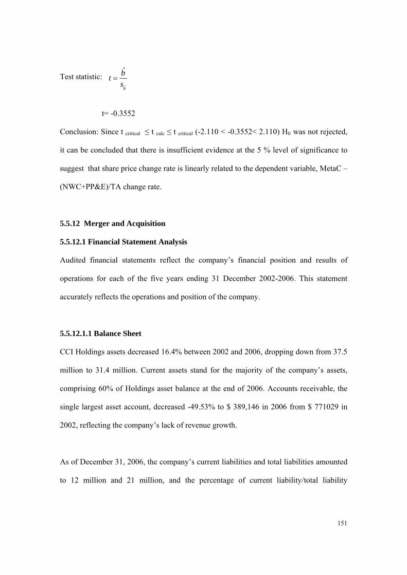
151

Test statistic:

t= -0.3552

Conclusion: Since t critical ≤ t calc ≤ t critical (-2.110 < -0.3552< 2.110) H0 was not rejected,

it can be concluded that there is insufficient evidence at the 5 % level of significance to

suggest that share price change rate is linearly related to the dependent variable, MetaC –

(NWC+PP&E)/TA change rate.

5.5.12 Merger and Acquisition

5.5.12.1 Financial Statement Analysis

Audited financial statements reflect the company’s financial position and results of

operations for each of the five years ending 31 December 2002-2006. This statement

accurately reflects the operations and position of the company.

5.5.12.1.1 Balance Sheet

CCI Holdings assets decreased 16.4% between 2002 and 2006, dropping down from 37.5

million to 31.4 million. Current assets stand for the majority of the company’s assets,

comprising 60% of Holdings asset balance at the end of 2006. Accounts receivable, the

single largest asset account, decreased -49.53% to $ 389,146 in 2006 from $ 771029 in

2002, reflecting the company’s lack of revenue growth.

As of December 31, 2006, the company’s current liabilities and total liabilities amounted

to 12 million and 21 million, and the percentage of current liability/total liability

ˆ

ˆ

b

bt

s

152

increased from 50% to 57% between 2002 and 2006, respectively. The current accounts

payable increased at 9.45% of the total revenue in 2006 from at 4.37% of the total

revenue in 2002.

As of December 31, 2006, long term liabilities totaled 32.75%, compared with 42.30% in

2002. Consistent with the company’s business long term growth strategy, leverage was

expected to keep the important component of the company’s capital structure.

Shareholder’s equity had decreased modestly since 2002 at 12 million, totaling $9 million

in 2006. And the equity represented 43% of the total liability, down from 52% as of

December 31, 2006. (See 5.34 Table)

5.5.12.1.2 Income Statement

CCI Holdings year to year revenue growth increased from 5.29% in 2002 ($42 million) to

13% in 2006, ($59 million), reflecting increased revenue associated with the increased

productivity. Operating expenses remained the stable relative to sales from 87.92% in

2002 to 87.64% in 2006. It can be seen that the operating expense represented the sales

was keeping the high percentage.

There is uneven growth in CCI Holdings net profit margin over the five years ending 31

December 2006. In particular, CCI Holdings net profit margin increased at 4.5% in 2002,

then it dramatically decreased at -16.5 % in 2003, -11.32% in 2004, -0.51% in 2005.

Following on from this period, the growth margin increased at 3.22% in 2006. According

to management’s growth and operating expectations for 2007 and 2008, the CCI

153

Holdings net profit margin was projected to approximate at 5% of sales in the following

years. (See 5.35 Table)

5.34 Table: CCI Holdings Limited Main Items in Annual Balance Sheet

2002 2003 2004 2005 2006-8,018,053 -8,409,802 -8,576,069 -8,090,637 -9,029,8041,763,362 1,396,794 3,198,654 1,578,821 6,384,2081,857,939 2,995,699 2,836,076 5,041,732 5,575,666

1,730,181 2,093,795 1,618,026 1,370,257 1,431,6336,709,133 7,525,803 7,244,820 8,706,498 9,913,9182,566,633 2,658,737 2,281,955 2,102,608 3,222,027

12,994,841 13,348,071 14,094,562 13,232,591 14,994,830771,029 1,547,896 1,320,543 59,513 389,146

-3,599,932 -3,829,658 -8,854,596 -17,478,618 -15,396,72016,596,846 16,770,165 20,042,878 24,575,770 24,858,17537,560,834 38,239,160 35,443,077 27,169,885 31,400,985

12,361,889 14,274,352 15,186,682 8,290,112 12,618,49511,507,159 11,934,602 14,001,050 14,575,976 18,835,27012,996,914 12,940,507 11,868,247 7,717,935 9,442,93824,563,920 25,298,653 23,574,830 19,451,950 21,958,04726,053,675 26,304,558 21,442,027 12,593,909 12,565,715

CCI Holdings Limited Main Idems In Annual Balanca Sheet

Total Curre AssetsTotal Equity

Total LiabilityTotal NCA

Retained Profit Share CapitalTotal Assets

Total CL

PP&EReceivables

Goodwill

Curr Accounts PayableCurrent Inventories

Debtors

Items/YearsAccumulated Depr

Cash

154

5.35 Table: CCI Holdings Limited Main Items in Annual Profit & Loss

2002 2003 2004 2005 2006-1,440,284 -1,717,485 -4,605,938 -4,038,849 -359,603-876,903 -975,824 -807,992 -1,828,685 -1,288,6722,932,686 485,167 331,013 1,142,333 5,475,1875,249,873 3,178,476 5,744,943 7,009,867 7,123,4621,742,225 -746,868 -1,649,460 -1,170,681 4,662,135

26,481 13,124 70,312 86,007 154,2650 615,185 -3,450,792 -7,407,235 -955,031

-4,641 39,052 72,000 -326,255 01,370,825 -844,908 -1,574,146 -1,216,787 3,664,4001,375,466 -268,775 -5,096,938 -8,297,767 2,709,369

-37,258,608 -41,577,964 -38,510,594 -45,205,008 -51,877,41938,262,364 40,918,559 43,305,183 51,602,659 58,500,5004,246,117 3,837,881 950,354 612,216 500,3811,370,825 -229,723 -5,024,938 -8,624,022 2,709,369

67,051 30,796 -280,201 124,129 -102,481-371,400 -98,040 75,314 -46,106 -1,230,259

42,508,481 44,756,440 44,255,537 52,214,875 59,000,881

CCI Holdings Limited Main Idems In Annual Profit & Loss

Other RevenueReported NPAT

Share of Associates Profit

NPAT Before AbsNPAT Pre-cap Profits

Operating ExpenseOperating Revenue

Net AbnormalsNet Capital Profit

Interest Revenue

Tax Expense

EBITEBITDA

EBT Before Abs

Total Revenue

Items/YearsAmortisationDepreciation

5.5.12.1.3 Ratio Analysis

Activity ratios indicated that CCI Holdings assets utilization was generally improving

over the five year ended 2006. In particular accounts receivable turnover and average

collection periods remained the stable during these periods. However, there are

dramatically increase in the asset turnover and working capital turnover between 2002

and 2006. The reason for that is the company’s accounts receivable and working capital

have significantly grew. Meanwhile, this phenomenon indicates that CCI Holdings was

utilising its asses more effectively.

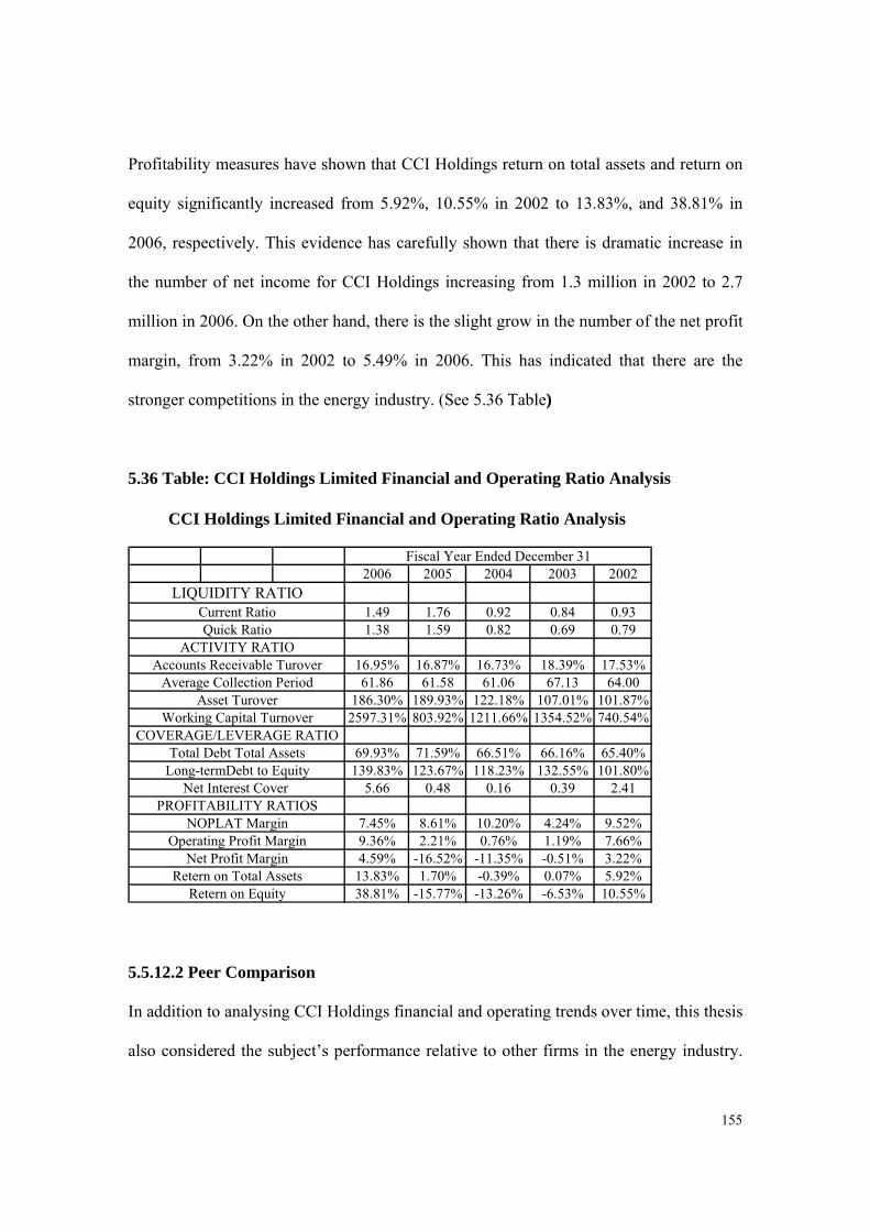
155

Profitability measures have shown that CCI Holdings return on total assets and return on

equity significantly increased from 5.92%, 10.55% in 2002 to 13.83%, and 38.81% in

2006, respectively. This evidence has carefully shown that there is dramatic increase in

the number of net income for CCI Holdings increasing from 1.3 million in 2002 to 2.7

million in 2006. On the other hand, there is the slight grow in the number of the net profit

margin, from 3.22% in 2002 to 5.49% in 2006. This has indicated that there are the

stronger competitions in the energy industry. (See 5.36 Table)

5.36 Table: CCI Holdings Limited Financial and Operating Ratio Analysis

2006 2005 2004 2003 2002

1.49 1.76 0.92 0.84 0.931.38 1.59 0.82 0.69 0.79

16.95% 16.87% 16.73% 18.39% 17.53%61.86 61.58 61.06 67.13 64.00

186.30% 189.93% 122.18% 107.01% 101.87%2597.31% 803.92% 1211.66% 1354.52% 740.54%

69.93% 71.59% 66.51% 66.16% 65.40%139.83% 123.67% 118.23% 132.55% 101.80%

5.66 0.48 0.16 0.39 2.41

7.45% 8.61% 10.20% 4.24% 9.52%9.36% 2.21% 0.76% 1.19% 7.66%4.59% -16.52% -11.35% -0.51% 3.22%

13.83% 1.70% -0.39% 0.07% 5.92%38.81% -15.77% -13.26% -6.53% 10.55%

CCI Holdings Limited Financial and Operating Ratio Analysis

Fiscal Year Ended December 31

Net Profit Margin

Total Debt Total AssetsLong-termDebt to Equity

Net Interest Cover

Average Collection Period

Working Capital TurnoverAsset Turover

LIQUIDITY RATIOCurrent RatioQuick Ratio

ACTIVITY RATIOAccounts Receivable Turover

COVERAGE/LEVERAGE RATIO

Retern on EquityRetern on Total Assets

PROFITABILITY RATIOSNOPLAT Margin

Operating Profit Margin

5.5.12.2 Peer Comparison

In addition to analysing CCI Holdings financial and operating trends over time, this thesis

also considered the subject’s performance relative to other firms in the energy industry.

156

CCI Holdings financial condition and operating performance were compared to similarly

sized energy industry companies. It can be seen that from the common size comparison

of CCI Holdings and selected guideline transactions balance sheet, the subject company

was similar to the average of selected guideline transactions. In addition, there was slight

decrease at -16.40% in CCI Holdings total assets from 2002 to 2006, but the number of

total assets for selected guideline transactions increased at 4.7% in the same periods. The

number of total liability decreased by 10.7% for CCI Holdings and increased by 61% for

selected guideline transactions.

A common size comparison of the subject’s income statements and selected companies

income statements reveal that the number of operating expense have increased rapidly at

39% and 81% for the subject and selected companies from 2002 to 2006. In the addition,

there was dramatic grow in the number of total revenue at 99% and slight increase at 38%

for the selected company and subject company in the same periods.

An analysis of CCI Holdings financial and operating rations relative to the selected

companies indicated that there were similar current ratios for the subject company and

selected companies at 1.49 and 1.76 in 2006, respectively. Compared to this situation,

CCI Holding quick ratio was 1.38 and the selected guideline transactions were 1.59. The

most notable differences between the subject and those firms were the net profit margin;

CCI Holding was 3.22% in 2002 and slight increased to 4.59% in 2006. But, there were

dramatic increase in the net profit ratio for the selected guideline transactions, growing

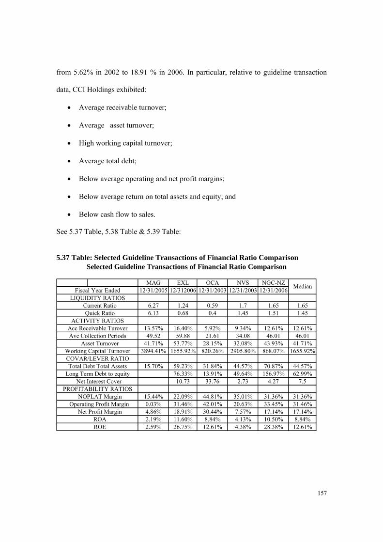
157

from 5.62% in 2002 to 18.91 % in 2006. In particular, relative to guideline transaction

data, CCI Holdings exhibited:

Average receivable turnover;

Average asset turnover;

High working capital turnover;

Average total debt;

Below average operating and net profit margins;

Below average return on total assets and equity; and

Below cash flow to sales.

See 5.37 Table, 5.38 Table & 5.39 Table:

5.37 Table: Selected Guideline Transactions of Financial Ratio Comparison

MAG EXL OCA NVS NGC-NZ12/31/2005 12/312006 12/31/2003 12/31/2003 12/31/2006

6.27 1.24 0.59 1.7 1.65 1.656.13 0.68 0.4 1.45 1.51 1.45

13.57% 16.40% 5.92% 9.34% 12.61% 12.61%49.52 59.88 21.61 34.08 46.01 46.01

Asset Turnover 41.71% 53.77% 28.15% 32.08% 43.93% 41.71%3894.41% 1655.92% 820.26% 2905.80% 868.07% 1655.92%

15.70% 59.23% 31.84% 44.57% 70.87% 44.57%76.33% 13.91% 49.64% 156.97% 62.99%

Net Interest Cover 10.73 33.76 2.73 4.27 7.5

15.44% 22.09% 44.81% 35.01% 31.36% 31.36%0.03% 31.46% 42.01% 20.63% 33.45% 31.46%4.86% 18.91% 30.44% 7.57% 17.14% 17.14%2.19% 11.60% 8.84% 4.13% 10.50% 8.84%2.59% 26.75% 12.61% 4.38% 28.38% 12.61%

Selected Guideline Transactions of Financial Ratio Comparison

LIQUIDITY RATIOS

ACTIVITY RATIOS

COVAR/LEVER RATIO

PROFITABILITY RATIOS

Fiscal Year EndedMedian

NOPLAT Margin

Working Capital Turnover

Current Ratio Quick Ratio

Acc Receivable TuroverAve Collection Periods

ROE

Operating Profit Margin Net Profit Margin

ROA

Total Debt Total AssetsLong Term Debt to equity

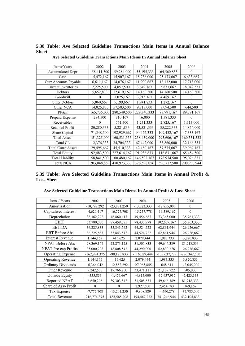
158

5.38 Table: Ave Selected Guideline Transactions Main Items in Annual Balance Sheet

Items/Years 2002 2003 2004 2005 2006Accumulated Depr -58,411,500 -59,284,000 -55,195,333 -64,560,833 0

Cash 15,472,167 15,907,167 15,736,000 25,173,667 6,633,667Curr Accounts Payable 6,611,167 14,076,167 11,900,667 18,132,000 17,713,000

Current Inventories 2,225,500 4,057,500 3,649,167 5,837,667 18,042,333Debtors 5,652,833 12,619,167 14,160,500 14,160,500 14,160,500

Goodwill 0 1,025,167 3,915,167 4,489,167 0Other Debtors 5,860,667 5,199,667 1,941,833 1,272,167 0

Other NCA 14,025,833 57,583,500 9,818,000 8,094,500 644,500PP&E 165,735,000 280,549,500 229,340,333 89,791,167 89,791,167

Prepaid Expense 284,500 310,167 16,000 1,581,333 0Receivables 0 761,500 1,231,333 2,825,167 1,313,000

Retained Profit 20,280,333 5,221,833 -43,531,333 -35,222,333 14,854,000Share Capital 71,548,500 198,929,667 94,422,333 109,432,167 47,333,167Total Assets 151,325,000 160,531,333 238,439,000 295,606,167 160,531,333

Total CL 12,376,333 24,704,333 67,442,000 33,860,000 32,166,333Total Curre Assets 29,495,667 45,510,333 42,480,167 57,575,667 39,969,167

Total Equity 92,483,500 227,614,167 91,936,833 116,631,667 65,454,500Total Liability 58,841,500 100,480,167 146,502,167 178,974,500 95,076,833

Total NCA 203,048,889 470,973,333 326,598,056 396,717,500 200,936,944

Ave Selected Guideline Transactions Main Idems In Annual Balance Sheet

5.39 Table: Ave Selected Guideline Transactions Main Items in Annual Profit & Loss Sheet

Items/ Years 2002 2003 2004 2005 2006

Amortisation -10,797,292 -23,871,250 -13,723,333 -12,855,000 0

Capitalised Interest -4,620,417 -16,727,708 -15,257,778 -16,389,167 0

Depreciation 38,362,292 46,860,417 49,456,667 73,365,000 135,763,333

EBIT 53,780,000 87,459,375 78,437,778 102,609,167 135,763,333

EBITDA 36,225,833 35,843,542 44,524,722 62,861,944 126,926,667

EBT Before Abs 36,225,833 35,843,542 44,524,722 62,861,944 126,926,667

Interest Revenue 1,144,167 415,625 2,079,444 1,983,333 3,820,833

NPAT Before Abs 28,369,167 22,273,125 31,505,833 49,646,389 81,718,333

NPAT Pre-cap Profits 35,000,208 18,808,542 44,290,000 62,830,278 126,926,667

Operating Expense -162,994,375 -98,125,833 -116,029,444 -138,637,778 -296,342,500

Operating Revenue 1,144,167 415,625 2,079,444 1,983,333 3,820,833

Ordinary Dividends -6,366,042 -12,882,292 -27,065,845 -648,611 -42,045,000

Other Revenue 9,242,500 17,766,250 33,471,111 21,109,722 505,000

Outside Equity -335,833 -1,476,667 -4,815,000 -12,937,917 -7,423,333

Reported NPAT 6,650,208 39,303,542 31,505,833 49,646,389 81,718,333

Share of Asso Profit 0 0 2,927,500 2,454,583 369,167

Tax Expense -7,772,708 -13,201,250 -9,808,889 -4,590,278 -37,785,000

Total Revenue 216,774,375 185,585,208 194,467,222 241,246,944 432,105,833

Ave Selected Guideline Transactions Main Idems In Annual Profit & Loss Sheet

159

5.5.12.3 Identification and application of valuation multiples

In conducting the preceding comparative analysis of CCI Holdings to the selected market

data we found that Bureau Veritas Australia Pty Ltd acquired all the shares in the

company in June 2007. It can be seen that the merger and acquired company data are for

controlling interest transactions. Therefore, historical financial data that we selected to

value the company’s common equity should be based on the market value of invested

capital (MVIC). Market multiples calculated for the purpose of pricing CCI Holdings

MVIC included:

MVIC/sales;

MVIC/EBITDA;

MVIC/EBIT;

MVIC/GCF.

In addition to considering multiples based on historical financial data, we have used

analysis estimates and revenue and expense projections discussed in the analysis of CCI

Holdings financial statements to prepare projected fiscal 2006 income statements for the

subject and the selected guideline transactions. It should also be stated that a comparison

of CCI Holdings financial condition, operating performance and ratios with that of the

selected guideline transactions were calculated using only end-of-year financial data.

(See 5.40 Tables)

MVIC Multiple Adjustments

The following sections summarise the analysis and subsequent weighting of the selected

MVIC multiples. There are organised according to the mature of the underlying data.

160

MVIC/sales Regression analysis was conducted using EBITDA/sales as the

independent variable and MVIC/sales as the dependent variable. The results of this model

were lower, as evidenced by an R2 to 46% and the t-stat is 1.6. Therefore, analysis of the

median selected guideline transactions multiple has been rejected. Due to CCI Holding

quite low return to sales and the very high operating expenses to the selected guideline

transactions, we decided to adjusted the median CCI Holdings multiple downward by

15%.

The resulting multiple received a weight of 25% due to the relatively low coefficient

variance.

MVIC/EBITDA CCI Holdings EBITDA represented to the sales was very low that

the median for the selected guideline companies, 12.35% versus 48.5%. It can be seen

that CCI Holdings 2006 EBITDA has increased by 1.62%, but there were huge increase

in the average of selected guideline transactions as 101.91%. Comparative financial

analysis indicated that CCI Holdings had the lower asset utilization and operating profit

than the average of the selected guideline companies. Therefore, we have decided to

reduce the median MVIC/EBITDA multiples by 20%.

Given the relatively low coefficient variance demonstrated by the MVIC/EBITDA

multiple, we will calculate this multiple a weight of 25%.

MVIC/EBIT Similarly, CCI Holdings very low net profit margin, operating profit

margin and the high risk of operating expenses make us to reduce the reported median

MVIC/EBIT multiple by 20% as well .

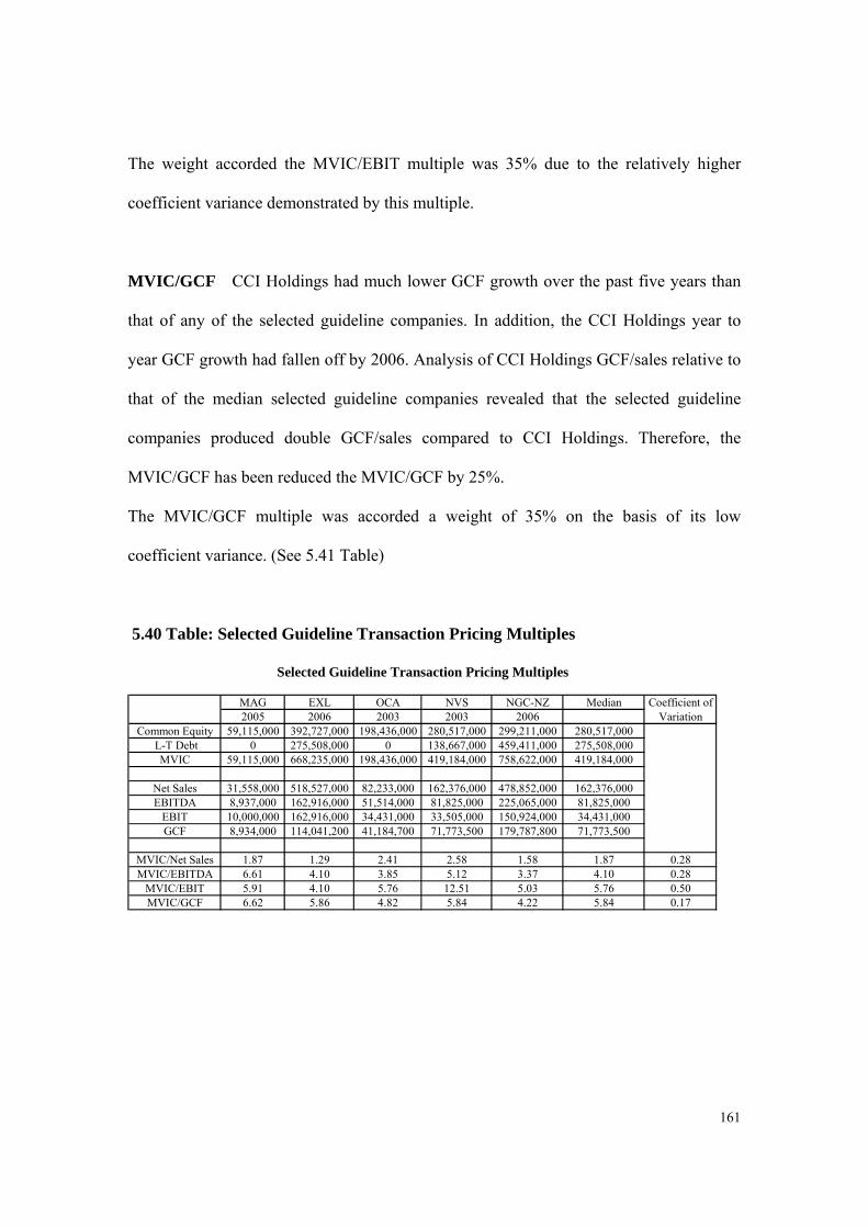
161

The weight accorded the MVIC/EBIT multiple was 35% due to the relatively higher

coefficient variance demonstrated by this multiple.

MVIC/GCF CCI Holdings had much lower GCF growth over the past five years than

that of any of the selected guideline companies. In addition, the CCI Holdings year to

year GCF growth had fallen off by 2006. Analysis of CCI Holdings GCF/sales relative to

that of the median selected guideline companies revealed that the selected guideline

companies produced double GCF/sales compared to CCI Holdings. Therefore, the

MVIC/GCF has been reduced the MVIC/GCF by 25%.

The MVIC/GCF multiple was accorded a weight of 35% on the basis of its low

coefficient variance. (See 5.41 Table)

5.40 Table: Selected Guideline Transaction Pricing Multiples

MAG EXL OCA NVS NGC-NZ Median Coefficient of2005 2006 2003 2003 2006 Variation

Common Equity 59,115,000 392,727,000 198,436,000 280,517,000 299,211,000 280,517,000 L-T Debt 0 275,508,000 0 138,667,000 459,411,000 275,508,000

MVIC 59,115,000 668,235,000 198,436,000 419,184,000 758,622,000 419,184,000

Net Sales 31,558,000 518,527,000 82,233,000 162,376,000 478,852,000 162,376,000EBITDA 8,937,000 162,916,000 51,514,000 81,825,000 225,065,000 81,825,000

EBIT 10,000,000 162,916,000 34,431,000 33,505,000 150,924,000 34,431,000GCF 8,934,000 114,041,200 41,184,700 71,773,500 179,787,800 71,773,500

MVIC/Net Sales 1.87 1.29 2.41 2.58 1.58 1.87 0.28MVIC/EBITDA 6.61 4.10 3.85 5.12 3.37 4.10 0.28

MVIC/EBIT 5.91 4.10 5.76 12.51 5.03 5.76 0.50MVIC/GCF 6.62 5.86 4.82 5.84 4.22 5.84 0.17

Selected Guideline Transaction Pricing Multiples

162

5.41 Table: Guideline Market Data MVIC Multiple Adjustments

Median Pricing Adjustment Adjusted Pric Multiple

Multiple Factor Multiple WeightGuideline Trans Data

MVIC/Net Sales 1.87 -15.00% 1.59 25.00%MVIC/EBITDA 4.10 -20.00% 3.28 25.00%

MVIC/EBIT 5.76 -20% 4.61 15.00%MVIC/GCF 5.84 -25% 4.38 35.00%

Guideline Market Data MVIC Multiple Adjustments

5.42 Table: Guideline Transaction Methods Weighting and MVIC Calculation

Therefore, the company’ share price equals to common equity / outstanding

CCI Holdings share price = 30,394,868/132,556,491

= $0.22

The control value base on guideline transaction common equity $ 30,394,868

The CCI Holdings share price is $0.32 in the financial reports

The CCI Holdings common equity is $40,400,000 in the financial reports

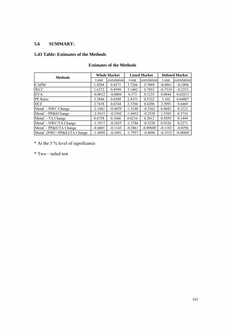
163

5.6 SUMMARY:

5.43 Table: Estimates of the Methods

t-stat correlation t-stat correlation t-stat correlationCAPM 1.8204 0.4371 3.7266 0.7069 -0.6861 -0.1804WCC 1.6372 0.4599 3.1482 0.7053 -0.7319 -0.2253EVA -0.0012 -0.0004 0.373 0.1235 0.0844 0.02813PE Ratio 3.3846 0.6588 2.4331 0.5322 3.102 0.64007DCF 2.7418 0.6744 2.3704 0.6208 2.3991 0.6469MetaC - NWC Change -2.1061 -0.4659 -1.5248 -0.3562 0.8683 0.2121MetaC - PP&EChange -2.5015 -0.5302 -1.0452 -0.2528 1.5505 0.3716MetaC - TA Change 0.6758 0.1666 0.8216 0.2012 0.5859 0.1449MetaC - NWC/TA Change -1.1917 -0.2855 -1.3786 -0.3258 0.9326 0.2271MetaC - PP&E/TA Change -0.4601 -0.1143 -0.3861 -0.09608 -0.1183 -0.0296MetaC (NWC+PP&E)/TA Change -1.4899 -0.3491 -1.7957 -0.4096 -0.3552 -0.08845

Estimates of the Methods

MethodsWhole Market Listed Market Delisted Market

* At the 5 % level of significance

* Two – tailed test

164

CHAPTER SIX

CRITIQUE AND DISCUSSION

165

6.1 Introduction

This chapter will critique seven business valuation methods’ efficiency for the

Australian energy sector. The chapter starts with a brief overview of seven business

valuation methods, and provides the methods application processes and the results. The

linear regression and t-test have been used to compare business valuation methods and

the share price, in order to obtain which method is better for evaluation business

performance in Australian energy sector.

6.2 CAPM

6.2.1 Overview of CAPM

Capital asset pricing model (CAPM) is a model of financial economics that is used to

measure the rate of return of an asset in a well-diversified portfolio, and thus determining

its value (Truong, 2008). Therefore, CAPM is a model used to determine the price of an

asset.

CAPM was introduced by Jack Treynor, Willian Sharpe, John Lintner and Jan Mossin

independently, building on the earlier work of Harry Markowitz on diversification and

modern portfolio theory (Truong, 2008). Under the capital asset pricing model, the price

of an asset is determined in accordance to its reward-to-risk ratio, where the reward is the

expected rate of return in the market and the risk is the asset’s non-diversifiable risk (β),

also referred to as systematic risk, or market risk (Truong, 2008) . The β here is the

166

measure of the risks involved in a particular stock or portfolio in relation to the overall

market risk.

6.2.2 Application of Method

Derived from this formula, the capital asset pricing model (CAPM) is expressed as:

E (R i) =R f+ i m (E(R m)-R f)

Where:

E (R i) is the expected return on the capital asset

R f is the risk-free rate of interest in the economy (for example, the yield on Treasury

bills or bonds).

Notes1: The risk-free interest rate is the interest rate that it is assumed can be obtained by

investing in financial instruments with no default risk.

i m (the beta coefficient) the sensitivity of the asset returns to market returns, or

also i m=( , )

( )

Cov Ri Rm

Var Rm

E(R m) is the expected return of the market

E(R m) - R f is sometimes known as the market premium or risk premium (the difference

between the expected market rate of return and the risk-free rate of return).

In this model, the Australian All Ordinaries Index end of year close from 1989 to 2007

has been used for the expected market rate of return and its rate of return is usually

measured by looking at the arithmetic average of the historical returns on a market

portfolio.

167

According to research by Truong (2008), the risk-free rate can be represent by 20-year,

5-year, or 30-day treasury or bonds yield as of valuation data. Therefore, the Australian

Government 10 yrs bonds rate end of year close from 1989 to 2007 (Year Book Australia,

2008) has been conducted for the risk free rate of return and it is usually the arithmetic

average of historical risk free rates of return and not the current risk free rate of return.

6.2.3 Empirical Results

Regression analysis has been used to develop an equation (a linear regression line) for

predicting a value of the dependent variables given a value of the independent variable.

Regression analysis formula is:

Y = a + b X

Where X is the independent variable (share price), Y is the dependent variable (CAPM),

a is the intercept and b is the slope of the line. For every fixed value of X, the E’S are

assumed to be independent random quantities normally distributed with mean zero.

6.2.3.1 T – Test Results

The t-test was conducted to show whether the means of the share price and CAPM are

statistically different from each other. This thesis selected the significant level at the 0.05

and two-tailed test in the whole market, listed market and delisted market to analyse the

relationship between them.

6.1 Table: t- test for CAPM

168

t-stat correlation t-stat correlation t-stat correlationCAPM 1.8204 0.4371 3.7266 0.7069 -0.6861 -0.1804

MethodsWhole Market Listed Market Delisted Market

It can be seen that CAPM is more highly associated with the share price in listed markets

and weak correlation with share price in delisted markets.

6.2.4 Strength and Weakness of CAPM

Lvkovic (2007) identifies the following three strength of CAPM:

CAPM is that it provides a precise and measurable definition of risk as applied to

stocks;

CAPM remains the most straight-forward and widely used quantitative tool for

estimating the cost of equity capital; and

CAPM is the idea that risk-return relation of every portfolio can be optimized to

attain lowest risk for a specific level of return.

Lvkovic (2007) also gives some following weakness to CAPM:

The model assumes that asset returns are normally distributed random variables. It

is however frequently observed that returns in equity and other markets are not

normally distributed. As a result, large swings occur in the market more

frequently than the normal distribution assumption would expect;

The model assumes that the variance of returns is an adequate measurement of

risk. This might be justified under the assumption of normally distributed returns,

169

but for general return distributions other risk measures will likely reflect the

investors’ preferences more adequately; and

Model does not appear to adequately explain the variation in stock returns.

Empirical studies show that low beta stocks may offer higher returns than the

model would predict.

6.2.5 Empirical Analysis

6.2.5.1 Based on the market value

CAPM is used to determine a theoretically appropriate required rate of return of an asset,

CAPM is expressed as: E (R i) =R f+ i m (E(R m)-R f). Here, R f is the risk-free rate of

interest in the economy, the Australian Government 10 yrs bonds rate end of year close

from 1989 to 2007 has been conducted for the risk free rate of return. E(R m) is the

expected return of the market, the Australian All Ordinaries Index end of year close from

1989 to 2007 has represented for the expected market rate of return E(Rm) - R f is

sometimes known as the market premium or risk premium, it is the return in excess of the

risk-free rate of return that an investment is expected to yield. An asset’s risk premium

is a form of compensation for investors who tolerate the extra risk, compared to that of a

risk-free asset in a given investment. The evidence shows that the CAPM model based on

the market value rather than the book value, it can exactly measure the rate of return of an

asset for the firms in the market. Therefore, CAPM is the higher associated with the share

price in the listed market.

170

6.2.5.2 Beta Affects CAPM

According to CAPM, beta is the only relevant measure of a stock’s risk. A share’s beta

factor is the measures of measure of its volatility in terms of market risk (Francis &

Grout, 2000). The beta factor of the market as a whole is 1.0. Market risk makes market

returns volatile and the beta factor is simply a yardstick against which the risk of other

investments can be measured. Risk or uncertainty describes a situation where there is not

first one possible outcome but array of potential returns. Risk is measured as the beta

factor or B (Francis & Grout, 2000).

The market as a whole has B = 1;

Risk free security has a B = 0;

A security with a B < 1 is lesser risky than average Market;

A security with a B > 1 has risk above market; and

A security with a B <0 has inversely follows the market and its.

6.2.5.3 Low Beta and Negative Beta Affect on CAPM

From the calculated results, there is only one year negative beta -0.2587 (1997) in the

listed companies and its average beta is 0.99 (excluded unusual 7.1158 in 1999). But,

delisted companies have 11 years’ negative beta, -0.2991 (1992), -0.2086 (1994), -0.0050

(1995), -0.1678 (1996), -1.7642 (1997), -0.2503 (1998), -2.7375 (2001), -2.7545(2002), -

1.1014(2003), -3.5075(2007) and its average beta is -0.77 (excluded unusual 6.5978 in

1999).

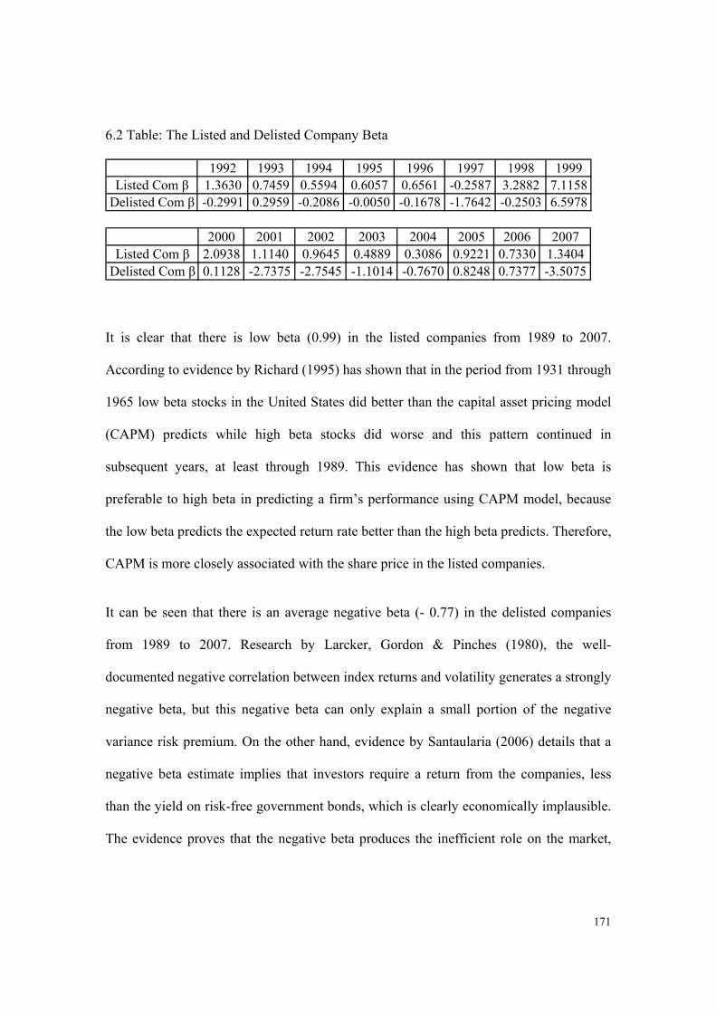
171

6.2 Table: The Listed and Delisted Company Beta

1992 1993 1994 1995 1996 1997 1998 1999Listed Com β 1.3630 0.7459 0.5594 0.6057 0.6561 -0.2587 3.2882 7.1158

Delisted Com β -0.2991 0.2959 -0.2086 -0.0050 -0.1678 -1.7642 -0.2503 6.5978

2000 2001 2002 2003 2004 2005 2006 2007Listed Com β 2.0938 1.1140 0.9645 0.4889 0.3086 0.9221 0.7330 1.3404

Delisted Com β 0.1128 -2.7375 -2.7545 -1.1014 -0.7670 0.8248 0.7377 -3.5075

It is clear that there is low beta (0.99) in the listed companies from 1989 to 2007.

According to evidence by Richard (1995) has shown that in the period from 1931 through

1965 low beta stocks in the United States did better than the capital asset pricing model

(CAPM) predicts while high beta stocks did worse and this pattern continued in

subsequent years, at least through 1989. This evidence has shown that low beta is

preferable to high beta in predicting a firm’s performance using CAPM model, because

the low beta predicts the expected return rate better than the high beta predicts. Therefore,

CAPM is more closely associated with the share price in the listed companies.

It can be seen that there is an average negative beta (- 0.77) in the delisted companies

from 1989 to 2007. Research by Larcker, Gordon & Pinches (1980), the well-

documented negative correlation between index returns and volatility generates a strongly

negative beta, but this negative beta can only explain a small portion of the negative

variance risk premium. On the other hand, evidence by Santaularia (2006) details that a

negative beta estimate implies that investors require a return from the companies, less

than the yield on risk-free government bonds, which is clearly economically implausible.

The evidence proves that the negative beta produces the inefficient role on the market,

172

which resulted in CAPM have a poor correlation with the share price in the delisted

market.

6.2.5.4 Share Price Change Rate Affects Beta The following is the share price change rate from 1989 to 2007, it is likely that delisted

companies have experienced dramatically change rate during this periods, from -37.55%

(1997-1998) to 235.4% (1991-1992). However, there are slight fluctuations in change

rate in the listed companies, between -24.41% (1997-1998) and 58.86% (1992-1993).

The beta is the average of 0.99 in the listed market and -0.77 in the delisted market. This

evidence has carefully shown that the beta is more accurately affects the market risk

under the moderate market condition; otherwise the beta is not able to measure the

companies’ undertaking risk and making CAPM misleading under stronger fluctuated

market.

6.3 Table: Share Price Change Rate for Listed and Delisted Company

1989-1990 1990-1991 1991-1992 1992-1993 1993-1994 1994-1995 1995-1996 1996-1997 1997-1998Lis Com -17.40% 6.11% 12.45% 58.86% 7.01% 20.78% 31.55% 9.44% -24.41%Delis Com -9.76% 62.70% 235.40% 22.40% -18.02% -25.12% 186.21% 24.50% -37.55%

1998-1999 1999-2000 2000-2001 2001-2002 2002-2003 2003-2004 2004-2005 2005-2006 2006-2007Lis Com 15.69% -1.05% 12.87% -0.55% 2.56% 52.72% 33.42% 41.98% 31.82%Delis Com -3.88% 63.05% 19.96% 1.97% 10.38% 99.54% 47.59% 14.45% 189.10%

Therefore, CAPM model is more highly associated with share price in listed market and

weak correlation with share price in delisted market. This is because the beta is the only

relevant measure of a stock’s risk. The low beta and negative beta have an essential role

in the CAPM.

173

6.3 WACC

6.3.1 Overview

The weighted average cost of capital is the rate that a company is expected to pay to

finance its assets. WACC is the minimum return that a company must earn on existing

asset base to satisfy its creditors, owners, and other providers of capital (Truong,

Partington, & Peat, 2008). The most obvious instance in which to use WACC is when the

objective is to value the entire capital structure of a company. WACC is especially

appropriate for project selection in capital budgeting. The proportions of debt and equity

that could be available to finance different kinds of project could be different and the cost

of capital should be based on the specific investment (Pratt, 1998).

6.3.2 Application of Method

The traditional formula used to develop a WACC is (Hitchner, 2006, p.190):

WACC= (K e*We) + (K p*W p) + (K d/ (pt) [1-t]*WD)

Where:

WACC= Weighted average cost of capital

K e = Cost of common equity capital

We = Percentage of common equity in the capital structure, at market value

K p = Cost of preferred equity

W p = Percentage of preferred equity in the capital structure, at market value

K d/(pt) = Cost of debt (pre tax)

T = Tax Rate

W d = Percentage of debt in the capital structure, at market value

174

According to Weighted Average Cost of Capital (2002, p. 6), regulatory decisions in

Australia have generally determined that the cost of equity is calculated using CAPM.

Therefore, the CAPM has been used for the cost of equity in this thesis.

The cost of debt in this thesis is measured as:

Total debt = long term debt + short term debt and current portion of long term

debt (Benninga, 2000);

Cost of debt = interest expense / total debt (Benninga, 2000).

The data of interest expense was only found on the database from 1996 to 2007, so the

WACC was calculated during this period.

Due to the lack of available information, the analysis on the cost of preferred equity has

been excluded. In addition, the cost of capital was expressed as a pre-tax real WACC in

this thesis.

6.3.3 Empirical Results

Regression analysis has been used to develop an equation (a linear regression line) for

predicting a value of the dependent variables (WACC) given a value of the independent

variable (Share Price).

6.3.3.1 T – Test Results

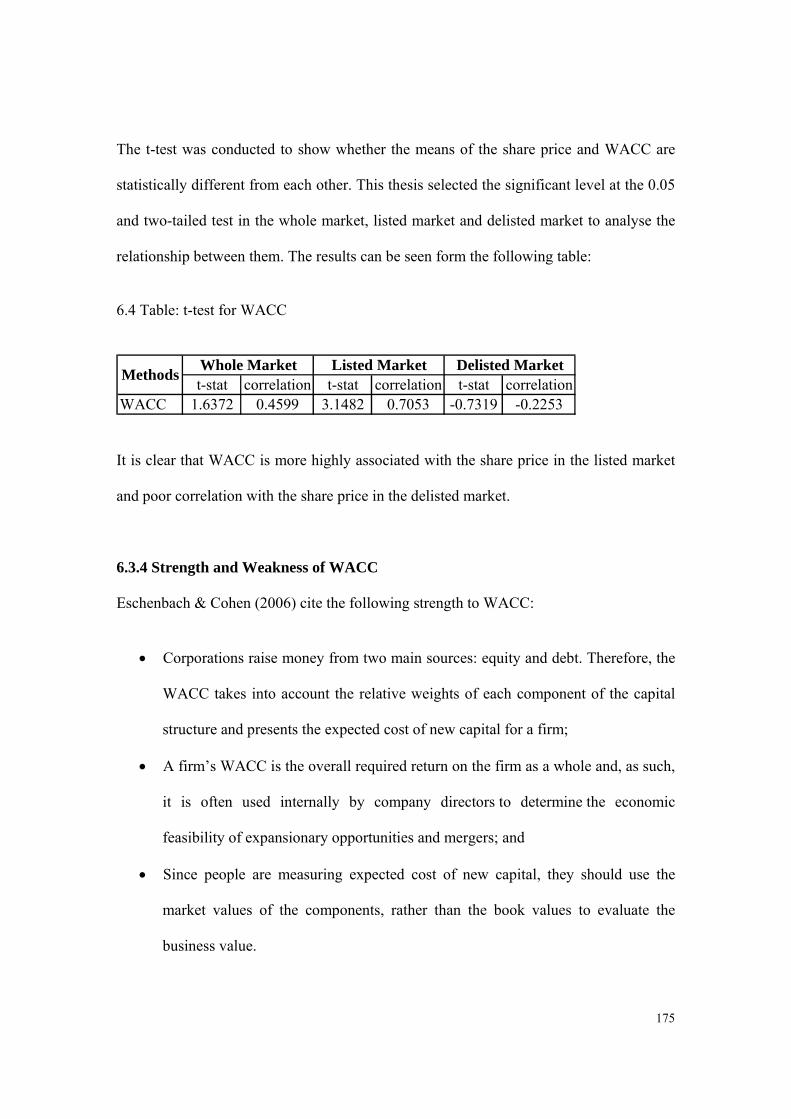
175

The t-test was conducted to show whether the means of the share price and WACC are

statistically different from each other. This thesis selected the significant level at the 0.05

and two-tailed test in the whole market, listed market and delisted market to analyse the

relationship between them. The results can be seen form the following table:

6.4 Table: t-test for WACC

t-stat correlation t-stat correlation t-stat correlationWACC 1.6372 0.4599 3.1482 0.7053 -0.7319 -0.2253

MethodsWhole Market Listed Market Delisted Market

It is clear that WACC is more highly associated with the share price in the listed market

and poor correlation with the share price in the delisted market.

6.3.4 Strength and Weakness of WACC

Eschenbach & Cohen (2006) cite the following strength to WACC:

Corporations raise money from two main sources: equity and debt. Therefore, the

WACC takes into account the relative weights of each component of the capital

structure and presents the expected cost of new capital for a firm;

A firm’s WACC is the overall required return on the firm as a whole and, as such,

it is often used internally by company directors to determine the economic

feasibility of expansionary opportunities and mergers; and

Since people are measuring expected cost of new capital, they should use the

market values of the components, rather than the book values to evaluate the

business value.

176

Also, Eschenbach & Cohen (2006) identify the following two weakness of WACC:

WACC is only applicable to assets that have the same systematic risks and

incremental debt ratio as the traded equity used to estimate its magnitude. In

general, for assets that do not meet this criterion, it is still necessary to estimate a

project-specific level of Kj; and

The premise of weighted average cost of capital is that an investor would pay no

more to purchase the asset than would be paid to reproduce the asset. While this

approach is suitable for some assets, particularly those which are not directly

generating income, choosing this approach as cost is not always a reliable guide to

value. For example, the vast amounts of money spent on pharmaceutical research

projects which come to nothing.

6.3.5 Empirical Analysis

The WACC is a weighted average of the cost of equity and debt. Regulatory decisions in

Australia have generally determined the cost of debt as a margin over the risk free rate,

while the cost of equity is calculated using CAPM (Weighted Average Cost of Capital

2002, p. 6).

The weighted average cost of capital (WACC) is used in finance to measure a firm’s cost

of capital. It has been used by many firms in the past as a discount rate for financed

projects, since the cost of the financing seems like a logical price tag to put on it (Truong,

Partington & Peat, 2008).

177

WACC is more closely associated with the share price in the listed market. This is

because when people are measuring expected cost of new capital, they should use the

market values of the components, rather than their book values (Truong, Partington &

Peat, 2008). From its traditional formula: WACC= (K e*We) + (K p*W p) + (K d/ (pt) [1-

t]*WD), it can be seen that the cost of equity and cost of debt (pre – tax) mainly consist of

WACC and both of them should be calculated by the market value. Market value is the

price at which an asset would trade in a competitive market and it reflects the market real

options (Galbraith & Stiles, 2008). The book value is value at which an asset is carried on

a balance sheet and it focus on the accounting measures. Therefore, using the market

value makes WACC model significant correlation with stock returns in listed market.

However, WACC model has a poor relationship with share price in a delisted market.

This is because estimated beta affects estimating WACC. According to evidence by the

Equity Beta of an Energy Distribution Business (2005), the estimated betas will vary

dramatically over time resulting in substantial swings in WACC estimates. In a

commercial setting, this would cause the firm’s investment strategy to be driven by

statistical aberrations in small data sets rather than economic fundamentals. “The

estimates could be dramatically different if a different data period, frequency, or

statistical method had been adopted” (The Equity Beta of an Energy Distribution

Business, 2005, p.65). These evidences have shown that the uncertainty surrounding beta

estimates and the effect this has on estimates of WACC. There is the negative beta in the

delisted market in the Australian energy sector, which resulted in weak relationship

between the stock returns and WACC in delisted market.

178

6.4 EVA

6.4.1 Overview

Evidence by Putnam (1997), Economic Value Added (EVA) is a trademark of the Stern

Stewart consulting organisation. Stern Stewart maintains that the implementation of a

complete EVA-based financial management and incentive compensation system gives

managers better information and superior motivation to make decisions that will create

the greatest shareholder wealth in any publicly-owned or private organisation.

EVA figures have also been conducted in the UK, Australia, Canada, Brazil, Germany,

Mexico, Turkey and France, and have been used to provide published rankings of

managerial performance, and several international companies have adopted EVA for

performance measurement in Australia. For example, the ANZ Banking Group, Fletcher

Challenge Limited, James Hardie Industries and the Wrightson Group have implemented

EVA financial management systems in recent years (Worthington, 2001).

6.4.2 Application of Method

EVA is essentially the surplus left after making an appropriate charge for the capital

employed in the business. It can be calculated in the following way (Economic Value

Added, 2007).

EVA = NOPAT – (TCE * WACC)

Where,

NOPAT = Net operating profit after tax

TCE = Total capital employed

179

WACC = Weighted average cost of capital

While calculation of NOPAT, the non-operating items will not be considered in these

steps. The total capital employed is the sum of shareholders funds as well as loan funds.

But this does not include investments outside the business (Economic Value Added,

2007).

In this thesis, the earnings before interest and taxes (EBIT) have been selected from the

database for the listed companies and delisted companies. We then should make the key

adjustments, for example, eliminating accounting distortions, and reclassifying some

expenses as investments as well as subtract cash operating taxes. Due to the data

limitation, we only adjusted one term, eliminating accounting distortions. Then invested

capital has been selected form the database and WACC has be found form the previous

work.

6.4.3 Empirical Results

Regression analysis has been used to develop an equation (a linear regression line) for

predicting a value of the dependent variables (EVA) given a value of the independent

variable (Share Price).

6.4.3.1 T – Test Results

The t-test was conducted to show whether the means of the share price and EVA are

statistically different from each other. We selected the significant level at the 0.05 and

180

two-tailed test in the whole market, listed market and delisted market to analyse the

relationship between them.

6.5 Table: t-test for EVA

t-stat correlation t-stat correlation t-stat correlationEVA -0.0012 -0.0004 0.3730 0.1235 0.0844 0.0281

MethodsWhole Market Listed Market Delisted Market

It is likely that EVA is weak correlation with share price in whole market, listed market

and delisted market.

6.4.4 Strength and Weakness of EVA

EVA is more than just a performance measurement system. It is also marketed as a

motivational, compensation-based management system that facilitates economic activity

and accountability at all levels in the firm (Grant, 2003).

Several strength claimed for EVA (Grant, 2003):

EVA eliminates economic distortions of GAAP to focus decisions on real

economic results;

EVA provides for better assessment of decisions that affect balance sheet and

income statement or tradeoffs between each through the use of the capital charge

against NOPAT;

EVA decouples bonus plans from budgetary targets;

EVA covers all aspects of the business cycle; and

181

EVA aligns and speeds decision making, and enhances communication and

teamwork.

Listed below are the weaknesses of EVA (Bartunek, 2007):

Unless fully loaded and all cash adjustments are made, economic profit can be

subject to accrual distortions. For example, because NOPAT is after depreciation

and amortization, a company that does not reinvest capital to maintain its plant

and equipment can improve its accrual bottom line simply by virtue of the

declining D&A line. This sort of attempt at boosting economic profit is known as

harvesting the assets; and

It has the limitations of any single-period, historical metric: last year’s economic

profit will not necessarily give you an insight into future performance. This can be

especially true if a company is in a turnaround situation or makes a large lump-

sum investment, in which case, economic profit will immediately suffer (due to

the higher invested capital base) but the expected future period payoff will not

show up as a benefit in the calculation.

6.4.5 Empirical Analysis

From the regression analysis, the EVA was the poor associated with the share price in the

whole market, listed market and delisted market. The reasons for which, will be

examined below.

EVA is considered as the centre-piece of a completely integrated financial framework for

financial management and incentive compensation (Steward, 1994). And EVA is

182

calculated as the business multiplied by the spread between the rate of return on capital,

defined as r, and the cost of capital, defined as c* ( Stewart, 1991).The evidence has

shown that EVA is an accounting-based measure of operating performance. So it is one

last limitation of EVA is that is still based on accounting figures, irrespective of the

GAAP- related adjustments (Worthington, 2001).

To define and refine its EVA measure, Stern Stewart & Co has identified a total of 164

performance measurement issues, including methods of addressing shortcomings in

conventional accounting such as: inventory costing and valuation, seasonality,

depreciation, revenue recognition, the write off of bad debts, the capitalisation and

amortisation of R&D, intangibles, mandated investments in safety and environmental

compliance, valuation of contingent liabilities and hedges, special issues for taxation,

inflation, currency translation, etc. (Stewart, 1994).

Nevertheless, because of the great number of possible adjustments, no company is

intended to apply all of them (Stewart, 1994; Stern, 1995; Ehrbar 1998). In general, they

found it necessary to address only 20 to 25 key measurement issues in detail and as few

as 5 to 10 key adjustments to be actually made in practice. Young (1999) argued that

many of the adjustments are of little importance to the company level, and some may be

difficult and costly as well, if not impossible, to replicate at the security level. Finally,

Young (1997, p. 338) summarizing the critique on the adjustment processing suggested

as a rule that ‘adjustments should be made only if the amounts are significant, the

required information is readily available, and no finance professionals can understand

them’.

183

Evidence by Keys, Azamhuzjaev and Mackey (2001), the general limitations for EVA are

as follows. Managers will have fewer choices in financing operations, risky projects will

be accepted and moderate ones will be rejected, EVA is too complex, EVA

is easy to

manipulate, EVA is a short term measure, EVA

is a single performance measure that

includes no measures for quality or time, EVA terminology is misleading, and EVA

should not be used for capital budgeting.

Therefore, EVA is an accounting-based measure of operating performance. It has

complex and costly accounting adjustments problems. In addition, these are not

consistent with standards for the EVA accounting adjustments, and the companies that

used the EVA to evaluate the performance have not revealed the processes for the using

the EVA.

6.5 DCF

6.5.1 Overview

Discounted Cash Flow (DCF) analysis is the technique used to derive economic and

financial performance criteria for investment projects (Herbohn & Harrison, 2008), and it

is a cash flow summary that has been adjusted to reflect the time value of money (Moses,

2008). Discounted cash flow was first formally published in 1938 in a text by John Burr

Williams: ‘The Theory of Investment Value’. This was after the market crash of 1929

and before auditing and public accounting was mandated by the SEC. Due to the

economic crash, investors were wary of relying on the reporting earnings, or in fact any

184

measures of value apart from cash (Discounted Cash Flow - DCF, 2008). Therefore,

discounted cash flow analysis gained popularity as a valuation method for stocks.

6.5.2 Application of Method

Middleton describes (2008) that discounted cash flow tries to calculate the value of a

company today. Ten listed energy companies (CEY, ERA, HED-NZ, OSH, STO, WPL,

NHC, AZA, BNT and PVE) and five delisted energy companies (BSO, CHL, NGC-NZ,

NVS and OCA) have been selected to calculate the company’s fair value using DCF and

will project cash flows for the next five years of business. The criteria for choosing the

companies is that the companies were keeping strong marketing channels, outstanding

growth, efficient factories and reasonable competitive position.

This thesis has decided to estimate the free cash flow that the selected companies will

produce over the next five years. Forecasting each of the companies revenue is the most

important assumption one that decides the company’s free cash flow.

We have got companies average revenue growth rate at 15% for the past 10 years and the

companies will keep at 10% in the future five years. Then we calculated the past 10 years

average operating costs margin of 65%, in order to get the operating costs. We assume

that the net investment is 10% of the revenue and the working capital has increased by

10% each year.

So the free cash flow can be calculated as the following (Benninga 2000, p. 65):

185

Free Cash Flow = Sales Revenue – Operating Costs – Taxes – Net Investment – Change

in Working Capital

After that we should calculate the terminal value approach that involves making some

assumptions about long-term cash flow growth (Benninga 2000, p.70).

Terminal Value = Final Projected Year Cash Flow X (1+Long-Term Cash Flow Growth Rate)

(WACC – Long-Term Cash Flow Growth Rate

In this formula, let’s assume that the company’s cash flows will grow in perpetuity by 4%

per year.

Then the enterprise value of the firms is the discounted value of the firm’s projected FCF

plus its terminal value (Benninga 2000, p. 72):

Enterprise value= FCF1/ (1+WACC) 1+FCF2/ (1+WACC) 2+……………………...

FCF5/ (1+WACC) 5+Year 5 terminal value/ (1+WACC)

Finally, we should deduct its net debt from the value to calculate the companies’ fair

value of equity.

6.5.3 Empirical Results

Regression analysis has been used to develop an equation (a linear regression line) for

predicting a value of the dependent variables (DCF) given a value of the independent

variable (Share Price).

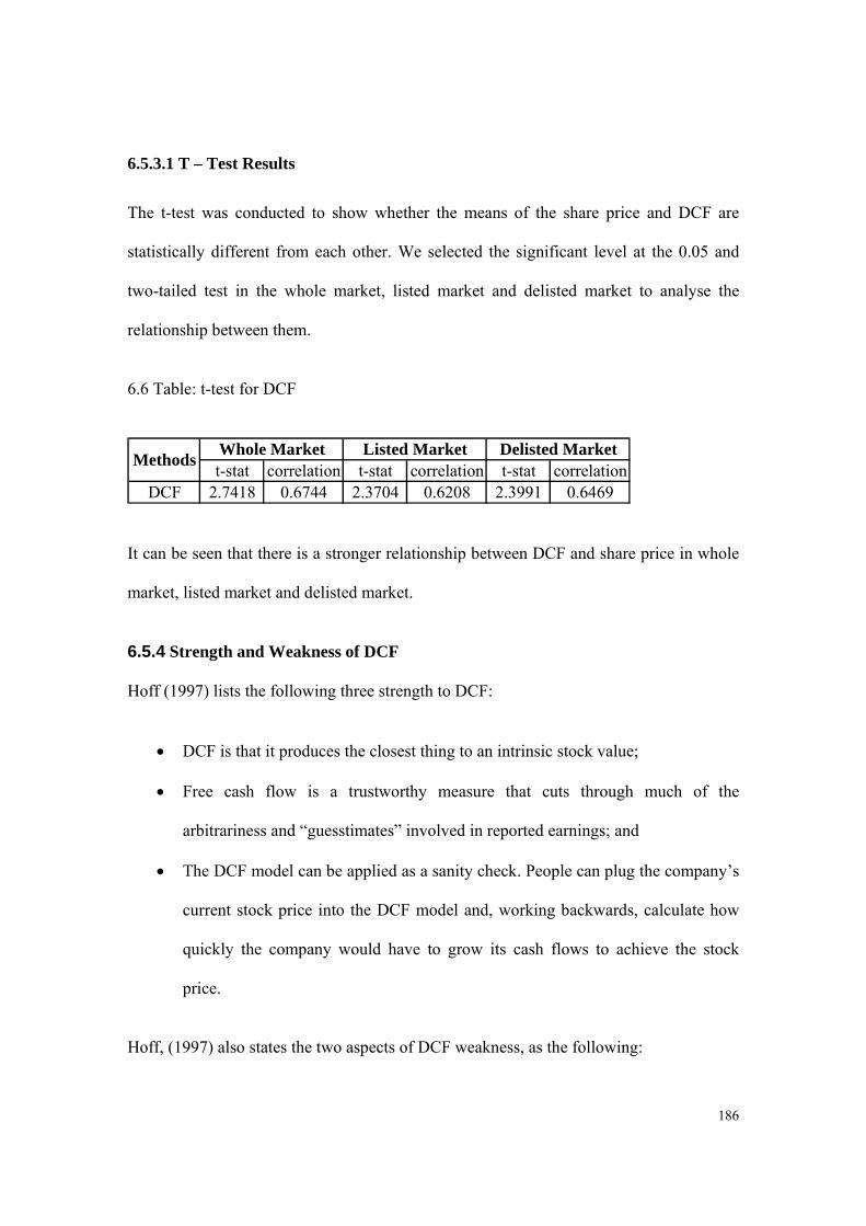
186

6.5.3.1 T – Test Results

The t-test was conducted to show whether the means of the share price and DCF are

statistically different from each other. We selected the significant level at the 0.05 and

two-tailed test in the whole market, listed market and delisted market to analyse the

relationship between them.

6.6 Table: t-test for DCF

t-stat correlation t-stat correlation t-stat correlationDCF 2.7418 0.6744 2.3704 0.6208 2.3991 0.6469

MethodsWhole Market Listed Market Delisted Market

It can be seen that there is a stronger relationship between DCF and share price in whole

market, listed market and delisted market.

6.5.4 Strength and Weakness of DCF

Hoff (1997) lists the following three strength to DCF:

DCF is that it produces the closest thing to an intrinsic stock value;

Free cash flow is a trustworthy measure that cuts through much of the

arbitrariness and “guesstimates” involved in reported earnings; and

The DCF model can be applied as a sanity check. People can plug the company’s

current stock price into the DCF model and, working backwards, calculate how

quickly the company would have to grow its cash flows to achieve the stock

price.

Hoff, (1997) also states the two aspects of DCF weakness, as the following:

187

The DCF model is only as good as its input assumptions. Depending on what you

believe about how a company will operate and how the market will unfold, DCF

valuations can fluctuate wildly; and

DCF works best when there is a high degree of confidence about future cash

flows. But things can get tricky when a company’s operations lack what analysts

call “visibility”. This is simple meant to mean, when it is difficult to predict sales

and cost trends with any certainty.

6.5.5 Empirical Analysis

At the present, DCF techniques have become the most popular techniques in making

capital budgeting decisions for public companies in Australia, as well as in other

countries (Kaplan & Ruback, 1995). In this thesis, the free cash flow to equity approach

has been used to analyse the energy companies’ fair value. Through the long term

analysis on this model, the t-stat is 2.7418, 2.3704 and 2.3991, respectively in whole

market, listed market and delisted market. The evidence has shown that using DCF model

is appropriate for the energy sector in the Australia.

It is clear that DCF analysis tries to work out the value of a company today, based on

projections of how much money it will generate in the future. The basic idea is that the

value of any company is the sum of the cash flows that it produces in the future,

discounted to the present at an appropriate rate (Lehn & Poulsen, 1989). Moreover, the

model is not suited to short-term investing, the DCF focuses on long-term value. A well-

crafted DCF may help you avoid buying into a bubble, but it may also make you miss

short-term share price run-ups that can be profitable (Lehn & Poulsen, 1989).

188

According to the evidence by Buckley (2002), DCF used the market values to measure

expected cost of new capital, rather than their book values, and it is based on realistic

rather than optimistic growth expectations. For the most part, free cash flow is a

trustworthy measure that cuts through much of the arbitrariness of “guesstimates”

involved in reported earnings (Farisssi, 2008).

On the other hand, DCF model produces the closest thing to an intrinsic stock value. The

alternatives to DCF are relative valuation measures, which uses multiples to compare

stocks within a sector (Morris, 2008). While relative valuation metrics such as price-

earnings (P/E), EV/EBITDA and price-to-sales ratios are fairly simple to calculate, they

are not very useful if an entire sector or market is over or undervalued. A carefully

designed DCF, by contrast, should help investors steer clear of companies that look

inexpensive against expensive peers (Morris, 2008).

The DCF model used the market values to measure expected cost of new capital rather

than their book values and DCF model produces the closest thing to an intrinsic stock

value. Therefore, the DCF model is suitable measure for the energy sectors in the long

term in Australia.

6.6 P/E ratio

6.6.1 Overview

The Price to Earnings (P/E) ratio is one of the oldest and most commonly used valuations

metric by investors to help determine whether individual stocks are reasonably priced

(Leibowitz & Kogelman, 1990). P/E is short for the ratio of a company’s share price to its

per-share earnings. The price per share is the market price of a single share of the stock.

189

The earnings per share is the net income of the company for the most recent 12 month

period, divided by number of shares outstanding. The P/E ratio can also be calculated by

dividing the company’s market capitalization by its total annual earnings (Maiello, 2008).

Theoretically, a stock’s P/E tells us how much investors are willing to pay per dollar of

earnings. For this reason it’s also called the “multiple” of a stock. In other words, a P/E

ratio of 20 suggests that investors in the stock are willing to pay $20 for every $1 of

earnings that the company generates (Minter & Weinter, 2008). Historically, the average

P/E ratio in the market has been around 15-25. This fluctuates significantly depending on

economic conditions. The P/E can also vary widely between different companies

andindustries (Minter & Weinter, 2008).

6.6.2 Application of Method

The P/E ratio formula is set as the following (Price-Earnings-Ratio, 2007):

P/E ratio = Price per Share

Annual Earning per Share

The price per share is the market price of a single share of the stock;

The earnings per share are the net income of the company for the most recent 12

month period, divided by number of shares outstanding.

P/E ratio is short for the ratio of the companies share price to its per-share earning. The

listed companies and delisted companies have been chosen to calculate the P/E ratio. In

the EPS calculation, the weighted average number of shares outstanding over the

reporting term has been used, in order to get more accurate EPS. It is very interesting

from the following table; there are a bigger different P/E ratio for listed companies from

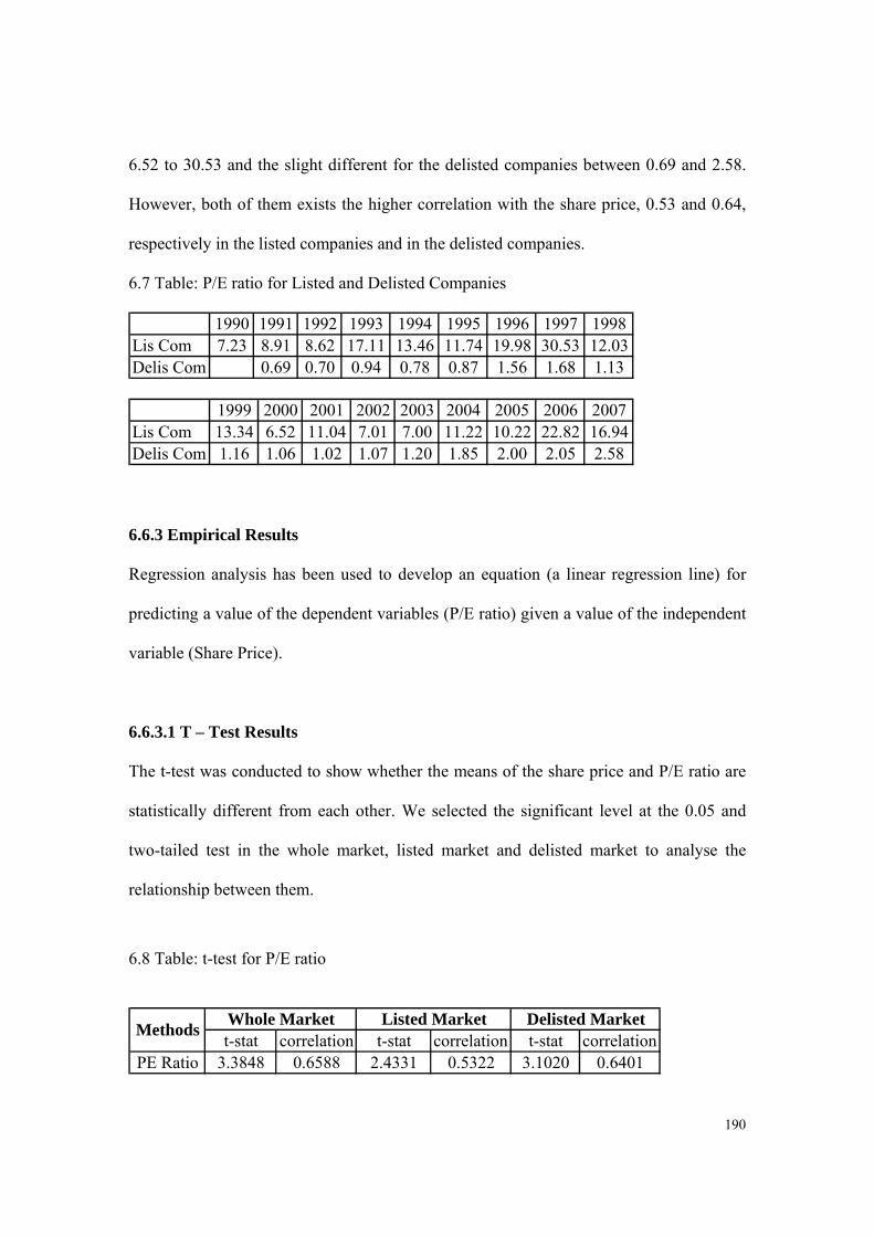
190

6.52 to 30.53 and the slight different for the delisted companies between 0.69 and 2.58.

However, both of them exists the higher correlation with the share price, 0.53 and 0.64,

respectively in the listed companies and in the delisted companies.

6.7 Table: P/E ratio for Listed and Delisted Companies

1990 1991 1992 1993 1994 1995 1996 1997 1998Lis Com 7.23 8.91 8.62 17.11 13.46 11.74 19.98 30.53 12.03Delis Com 0.69 0.70 0.94 0.78 0.87 1.56 1.68 1.13

1999 2000 2001 2002 2003 2004 2005 2006 2007Lis Com 13.34 6.52 11.04 7.01 7.00 11.22 10.22 22.82 16.94Delis Com 1.16 1.06 1.02 1.07 1.20 1.85 2.00 2.05 2.58

6.6.3 Empirical Results

Regression analysis has been used to develop an equation (a linear regression line) for

predicting a value of the dependent variables (P/E ratio) given a value of the independent

variable (Share Price).

6.6.3.1 T – Test Results

The t-test was conducted to show whether the means of the share price and P/E ratio are

statistically different from each other. We selected the significant level at the 0.05 and

two-tailed test in the whole market, listed market and delisted market to analyse the

relationship between them.

6.8 Table: t-test for P/E ratio

t-stat correlation t-stat correlation t-stat correlationPE Ratio 3.3848 0.6588 2.4331 0.5322 3.1020 0.6401

MethodsWhole Market Listed Market Delisted Market

191

It is likely that there are stronger relationships between share price and P/E ratio in whole

market, listed market and delisted market.

6.6.4 Strength and Weakness of P/E ratio

Henderson & Gart (1999) state the three aspects of P/E ratio strength, as the following:

P/E ratio is best viewed over time, looking for a trend. A company with a steadily

increasing P/E is being viewed by the investment community as becoming more

and more speculative. A company’s P/E ratio changes every day as the stock

price fluctuates;

P/E ratio is commonly used as a tool for determining the value of the market has

placed on a common stock. Companies expected to grow and have higher

earnings in the future should have a higher P/E than companies in decline; and

The P/E ratio is a much better indicator of a stock’s value than the market price

alone.

Sayeed (2008) states the four aspects of P/E ratio weakness, as the following:

The denominator (earnings) is based on an accounting measure of earnings that is

susceptible to forms of manipulation, making the quality of the P/E only as good

as the quality of the underlying earnings number;

Accounting: there are too many methods to calculate the actual earnings per share

(EPS), such as primary EPS, diluted EPS, and headline EPS etc. Moreover, some

192

investors can use the different way to calculate may get confused between the

different types of EPS and thus reach a wrong P/E estimate;

Inflation: during the periods of high inflation, inventory and depreciation costs

may be understated because the replacement costs of goods and equipment rise

with the general level of prices. Thus, P/E ratio tend to be lower during times of

high inflation because the market sees earnings as artificially distorted upwards;

Besides earnings, there are other factors that affect the value of a stock. For

example:

o Brand - The name of a product or company has value. Brands such as

Coca-Cola are worth billions;

o Human Capital - A company’s employees and their expertise are should

add value to the company;

o Expectations - The stock market is forward looking. People buy a stock

because of high expectations for strong profits, not because of past

achievements; and

o Barriers To Entry - For a company to be successful in the long run, it must

have strategies to keep competitors from entering the industry.

All these factors will affect a company’s earnings growth rate. Because the P/E ratio uses

past earnings (trailing twelve months), it gives a less accurate reflection of these growth

potentials.

6.6.5 Empirical Analysis

193

We had the analysis on the energy industry in Australia through the long term periods.

The results have shown that there are a stronger relationship between share price and P/E

ratio in whole market, listed market and delisted market. Here, we will discuss the

phenomena why P/E ratio model has the stronger relationship with share price in the

three markets.

P/E ratio is frequently used as a tool to measure the market value. For example,

companies expected to grow and have higher earnings in the future should have a higher

P/E than companies in decline. In addition, P/E ratio is best viewed over time, looking for

a trend. A company with a steadily increasing P/E is being viewed by the investment

community as becoming more and more speculative.

However, from the P/E ratio formula we can find the some issues:

P/E ratio = Price per Share

Annual Earning per Share

The price per share is the market price of a single share of the stock. The earnings per

share are the net income of the company for the most recent 12 month period, divided by

number of shares outstanding. It is clear that the price per share is the current company

share price and based on the market value. However, an important problem that the

denominator (earnings) is based on an accounting measure of earnings that is susceptible

to forms of manipulation, making the quality of the P/E only as good as the quality of the

underlying earnings number (Johnson & Shirer, 2008). This evidence has carefully

shown that people can get into a lot of troubles by valuing stocks using only simple

indicators such as the P/E ratio, because the P/E ratio is based on the book value rather

194

than the market value and the companies can easily manipulate the earning per share to

make the quality of the P/E ratio. On the other hand, it is difficult to say whether a

particular P/E is high or low without taking into account growth rates and the industry.

Therefore, although the P/E ratio has some problems, such as the accounting measure of

earnings and the inflation issues, it is also the most commonly used valuations metric by

investors, because it is the indicator of the market value and easily to calculate.

6.7 Merger and Acquisition

6.7.1 Overview

Mergers and acquisition (M&A) have long existed in the world of the corporate

landscape. They first appeared in the late1800s in the United States with the activity of

the “robber barons,” followed by the consolidations of J.P. Morgan and others in the

early 1900s. Since then, there have been several waves of M&A activity in the United

States during the booming economy of the late1960s, in the controversial restructuring

wave of the mid-1980s, and most recently with the mega-deals signed during the late

1990s (Hitchner, 2006).

6.7.2 Application of Method

Guideline Merger and Acquisition Method involves the valuation ratios derived from

transactional pricing information that is related to the appropriate underlying financial

data of guideline companies, and then applied to the corresponding data of the subject

company to arrive at an indication of value (Hitcher 2006, pp.260). The analysis involves

195

the comparison of the respective qualitative and quantitative factors relating to the

company being valued to those of the guideline companies (Hitcher 2006, pp.280).

Evidence by Hitcher (2006, pp.270-271), at its simplest, the method requires only

multiplication and perhaps some subtraction. The basic format is (Hitcher 2006, p. 272):

Value subject = [( Price

Parameter ) comps*Parameter subject] – Debt Subject

Parameter might be sales, net incomes, book value.

6.7.3 Empirical Results

Market multiples calculated for the purpose of pricing CCI Holdings, MVIC included:

MVIC/sales

MVIC/EBITDA

MVIC/EBIT

MVIC/GCF

In addition to considering multiples based on historical financial data, we have used

analysis estimates and revenue and expense projections discussed in the analysis of CCI

Holdings financial statements to prepare projected fiscal 2006 income statements for our

subject and the selected guideline transactions. It should be stated that a comparison of

CCI Holdings financial condition, operating performance and ratios with that of the

selected guideline transactions were calculated using only end-of-year financial data.

Finally, the CCI Holdings common equity can be calculated through the analysis of

subject company and guideline companies data as the following:

196

CCI Holdings common equity is equal to $30,394,868

Therefore, the company’ share price is equal to common equity / outstanding

CCI Holdings share price = $30,394,868/132,556,491

=$ 0.22

The CCI Holdings common equity is $ 46,309,644 in the financial reports

The CCI Holdings share price is $ 0.32 in the financial reports

6.7.4 Strength and Weakness of M&A

Hitchner (2006) lists the following strength to M&A:

It is fairly simple to understand. Companies with similar product, geographic, or

financial situations should have similar pricing characteristics;

It uses actual simple to apply. The M&A approach derives estimates of value

from relatively simple financial ration, drawn from a group of similar companies;

It uses actual data. The estimates of value are based on actual stock prices or

transaction prices, not estimates based on a number of assumptions or judgments;

and

It includes the value of all of a business’s operating assets.

Hitchner (2006) also states the four aspects of M&A weakness, as the following:

No good guideline companies exist. This may be the biggest reason the approach

is not used in a valuation. The analyst may not able to find guideline companies

that are sufficiently similar to the subject;

197

Most of the important assumptions are hidden. Among the most important

assumptions in a guideline price multiple is the company’s expected growth in

sales or earnings;

The application of these data to the subject company is complex because of the

difficulty determining whether a transaction is truly comparable given the limited

information available in the database; and

It is not as flexible or adaptable as other approaches.

6.7.5 Empirical Analysis

6.7.5.1 How much is the business worth

Establishing an acceptable and realistic price for the acquired company is difficult.

Traditional appraisals by accountants depend on a profitable history of three to five years

of recent operations, plus a net worth value derived from the financial statements E and

F. In the absence of profits, the net worth becomes the basis for the selling price.

Therefore, acquirers often overpay in merger and acquisition transactions. The over-

payment results in the following phenomenon:

A reduction in the value of the buyer’s stockholders’ equity;

A dilution in the buyer’s ownership interest in a merger transaction;

A reduction of the buyer’s cash and credit resources available to make more

economically sound investments;

A loss of investor confidence. This is particularly true with regard to investors in

public companies; and

198

Increasing the buyer’s cost of capital.

Therefore, the detailed commonly used M&A approach that compared the subject

company with the selected guideline transactions companies through the analysis on the

financial statement, income statement and financial ratio to get the subject company’s

common equity, which method is essential for the acquire to use suitable price to buy the

company.

In this analysis, the control value based on guideline transaction common equity is

$30,394,868. The share price in the market is $0.22. However, CCI Holdings common

equity and share price are $46,309,644 and $ 0.32 respectively in the financial reports.

This evidence has shown that the investors should adjust the acquire plan to avoid the

overpay. Because there is overvalued in CCI Holdings value.

6.7.5.2 M&A efficiency in the market

Research by Farrel & Shapiro (2000) have carefully examined that virtually any

significant horizontal merger involves some loss of direct competition, and would thus be

at least slightly anti-competitive in the absence of all efficiencies. Accordingly, the

question of efficiencies need be explicitly reached only if a merger created substantial

competitive concern. “The efficiencies of M&A for firms are truly combined their core

hard-to-trade assets in new ways that lead to lower costs or improved quality and

productivity”(Farrel & Shapiro, 2000,p.54). The evidences prove that the firms generate

efficiencies for the M&A based on competition of economic scale and should reduce the

operating costs and improve the product quality to satisfy the customer’s needs.

199

The following we will analyze the M&A efficiencies in CCI Holdings case. Bureau

Veritas Australia Pty Ltd paid 55.0 cents per share (dispatched to shareholders on 5 July

2007) and there was also a fully franked dividend of 3.0 cents per share paid on the same

date to acquire CCI Holdings. The evidence has shown that this acquisition involved the

direct competitors and was not monopolistic behaviour. On the other hand, Bureau

Veritas Australia Pty Ltd had seen significant growth in the Pacific Zone region after this

acquisition, which helped to grow the Pacific Zone operations into a force of over 2000

employees, serving over 5000 clients across a network of over 40 offices. This

acquisition also helped to expand the Pacific Zone service portfolio to lead international

trade services for the mining and coal industries across Australia & New Zealand.

It can be seen from this evidence, Bureau Veritas Australia Pty Limited acquired the CCI

Holdings is efficiencies, because this acquisition based on the competition and the

company improved the productivity as well as decreased the cost for the products.

6.7.5.3 How to be a successful M&A

Disciplined acquirers can extract value from mergers and acquisitions. The following lists

companies how become successful merger and acquisition in business activities (Farrel &

Shapiro, 2000):

Consider only targets for which the companies can improve future free cash flow;

Excel in estimating overall value creation;

Maintain discipline during negotiation;

Rigorously plan and execute the integration; and

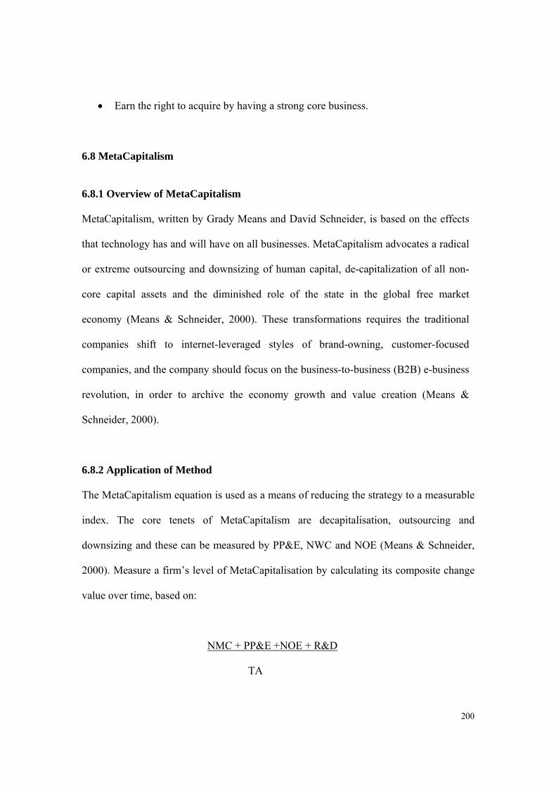
200

Earn the right to acquire by having a strong core business.

6.8 MetaCapitalism

6.8.1 Overview of MetaCapitalism MetaCapitalism, written by Grady Means and David Schneider, is based on the effects

that technology has and will have on all businesses. MetaCapitalism advocates a radical

or extreme outsourcing and downsizing of human capital, de-capitalization of all non-

core capital assets and the diminished role of the state in the global free market

economy (Means & Schneider, 2000). These transformations requires the traditional

companies shift to internet-leveraged styles of brand-owning, customer-focused

companies, and the company should focus on the business-to-business (B2B) e-business

revolution, in order to archive the economy growth and value creation (Means &

Schneider, 2000).

6.8.2 Application of Method

The MetaCapitalism equation is used as a means of reducing the strategy to a measurable

index. The core tenets of MetaCapitalism are decapitalisation, outsourcing and

downsizing and these can be measured by PP&E, NWC and NOE (Means & Schneider,

2000). Measure a firm’s level of MetaCapitalisation by calculating its composite change

value over time, based on:

NMC + PP&E +NOE + R&D

TA

201

Due to a lack of available information, the analysis on the NOE has been excluded. This

leaves six other indices to be tested. The original combined index was separated into the

following individual indices (Farrell, 2005):

NWC Change

PP & E Change

TA Change

NWC/TA Change

PP & E /TA Change

NWC +PP&E/TA Change

The formula is separated into six parts in order to compare with the change in the share

price. And to indicate some indices that are more responsible for such adverse effects

than others. And the period is the most significant as well as which MetaC indices change

is the most correlated to the share price change.

6.8.3 Empirical Results

Regression analysis has been used to develop an equation (a linear regression line) for

predicting a value of the dependent variables (NWC, PP&E, TA, NWC/TA, PP&E/TA

and NWC+PP&E/TA) given a value of the independent variable (Share Price). The

results have shown that the six dependent variables have the poor associated with the

share price. The following is the details about these results.

6.8.3.1 NWC+PP&E/TA Index

202

NWC+PP&E/TA are the other important index for the companies. This equation and in

particular the corresponding ratios, were taken to indicate the level of MetaCapitalisation

because they precisely represent the main tenets of the strategy-decapitalisation, selling

of physical assets, and reduction in the number of employees through downsizing and

outsourcing (Mickhail, Ostrovsky, 2005). According to the research study, the

NWC+PP&E/TA change correlation rate in the delisted companies is -18%, which was

negative correlation with the share price change. Due to MetaCapitalism strategies, when

the share price is the negative correlation with the NWC+PP&E/TA change, which can

make companies production more efficiency and bring more benefits for them. However,

in this case, collapse, mergers, taken over, suspended and down in rank groups was

included in the delisted company list. Therefore, these results contradict the claims of

MetaCapitalim.

6.8.3.2 Extreme Changes

Empirical reflections got the results that all the companies that were selected from each

group experienced the extreme changes in the total periods. For example, there was a

dramatic increase by 17729.41% in the TA change of CXR in 1990-1991, then the

change of TA significant decreased by 80.48% in 1991-1992 and continually dropped by

-14.51% in 1993-1994. Finally, the company went to bankruptcy in 1998. The other

example, the PP&E change of SPP was -28.26% in 1994-1995, -3517.97% in 1995-1996,

and then the change have dramatically increased by 4.01% in 1998-1999. At the last, the

company was closed in the year of 2000. Therefore, the most companies experienced the

203

extreme changes during the periods and then the companies quickly suffered the severe

damage.

6.8.3.3 Comparison with ASX 200 Energy Company

And the market clearly does consider PP&E to be important. PP&E was found to be the

single most important index for the individual companies (Farrell, 2005). Empirical

reflections have shown that most companies experienced the negative correlations with

ASX 200 Energy Company. For example, CXR, VOY, OMO, EXL and these companies’

PP& E were not consistent with the ASX 200 Energy Company. And these companies

experienced negative correlations with the share price when PP&E reduced. It is clear

that most PP&E change in the ASX 200 Energy Company was the positive correlation

with the share price change. Therefore, this evidence has shown that the ASX 200 Energy

Company PP&E change is the positive correlation with the share price change, which

refutes MetaCapitalism assumptions that decrease in PP&E change will increase the

share price change.

6.8.4 The Reason to Fail?

6.8.4.1 Value Added Communities

Value Added Communities are external network that address supply chain issues

involved in producing and delivering products (Means and Schneider, 2000). The

purpose of the VAC is to provide a central platform for members to interact that reduce

transaction costs by streamlining value chain processes. However, in the fact, there are

intensive competitions existed in the business market; it is unlikely that they will

204

cooperate together all of the time. Ostrovsky argues that the two main reasons why the

VACs do not function effectively. First, there are ‘insufficient trust and cooperation, and

a poor mix of firms if too much emphasis on selection is placed on competitive or

political reasons as posed to the firm’s ability to add value and generate wealth’

(Ostrovsky, 2003). Second, there is an ‘unrelenting quest for efficiency and market

dominance is facilitated by the ability of dominant firms to control smaller member forms

within the VACs, including deciding who to let in and on what terns, opportunities for

price manipulation and collusion within and between VACs, and the resulting

concentration and centralisation of capital and power’(Ostrovsky, 2003).

6.8.4.2 Outsourcing

Outsourcing is the transfer of the delivery of services which affects both jobs and

individuals. Downsizing results in increased local unemployment, which has

repercussions such as social dislocation, increased crime and poverty (Moore, 2002).

The social cost is very high where the pursuit of efficiency maximization is completely

disconnected from human well being (Gray, 2002). Although it is difficult to dispute that

outsourcing has a detrimental effect on individuals who face job disruption and

employment insecurity, it damages a local labour market and causes increased local

employment and social turbulent situation. These effects threaten social stability and

people’s lives.

6.9 Conclusion

205

According to data analysis and t-test for seven commonly used business valuation

methods over the long periods in the Australian energy sector, it can be seen that CAPM

and WACC have a close association with the share price in the listed market, and DCF

and P/E ratio have the higher correlation with the share price in the whole market, listed

market and delisted market. However, an important problem for P/E ratio is that the

denominator (earnings) is based on an accounting measure of earnings that is susceptible

to forms of manipulation, making the quality of the P/E only as good as the quality of the

underlying earnings figures. In addition, it is difficult to say whether a particular P/E is

high or low without taking into account growth rates and the industry. On the other hand,

the weighted average cost of capital (WACC) is used in finance to measure a firm’s cost

of capital. It has been used by many firms in the past as a discount rate for financed

projects, since the cost of the financing seems like a logical price tag to put on it.

Although the M&A method is good one for the companies to acquire and merger the

other companies, merger and acquisition do not conveniently occur on the effective date

if the subject company valuation. And the analyst may not be find guideline companies

that are sufficiently similar to the subject.

The survey sample by Truong & Partington (2006) has been found about business

valuation methods used in estimating the cost of capital in Australia in the different

sectors. The authors started with a sample of 488 stocks included in the All Ordinaries

Index as at August 2004. The focus of this survey is the capital budgeting practice of

Australian corporations; therefore the survey excluded all foreign companies. The final

sample comprises 356 companies in nine sectors. The survey results have shown that

206

CAPM was the most popular method of estimating the cost of capital in Australia with

73% of respondents relying mainly on the CAPM. The use of other asset pricing models

is virtually non-existent. In addition to the CAPM, this survey confirmed the popularity

of DCF methods in Australia with 75% of respondents used DCF techniques.

Therefore, the results can be achieved from the above analysis and shows that a CAPM is

a better method for the listed companies to measure the rate of return of an asset in a

well-diversified portfolio in Australian energy industry and DCF is better method for the

whole, listed and delisted companies to make capital budgeting decisions for public

companies in Australian energy sector.

207

CHAPTER SEVEN

LIMITATIONS AND FUTURE

RESEARCH

208

7.1 Limitations

Data Collection Problems Several problems were found in the stage of data collection. Firstly, each company

releases their financial statements at the different periods. Apart from the UOW resource,

it was necessary to check each company’s website to collect the company financial

statements. Nevertheless, sometimes the companies did not release their 2006-2007

annual reports either in company’s website or UOW website.

Secondly, due to a lack of available information, the analysis on the cost of preferred

equity has been excluded in the WACC formula. In addition, the data of interest expense

was only found on the database from 1996 to 2007, so the WACC was calculated during

this period.

Thirdly, measure a firm’s level of MetaCapitalisation by calculating its composite change

value over time, based on:

& &NWC PP E NOE R D

TA

Due to a lack of available information, the analysis on the NOE and R&D has been

excluded.

Data Adjustment Problems

To define and refine EVA measure, Stern Stewart & Co identified a total of 164

performance measurement issues. In addition, there were not consistent standards for the

209

EVA accounting adjustments, and the companies that used the EVA to evaluate the

performance have not revealed the processes for using the EVA. Due to data limitations,

the reclassifying some expenses are not included in the adjustment.

Problems to guideline companies’ transactions

Selected guideline companies for the M&A, the market data was collected by the

following criteria:

Similar business description or market;

Revenues between $ 1 million and $750 million;

Positive operating earnings for the latest reported fiscal year-end; and

Positive cash flow for the latest reported fiscal year-end.

Actually, the analyst may not able to find guideline companies that are sufficiently

similar to the subject.

7.2 Future research

The aims of this thesis are to explore the efficiency of business evaluation methods in the

energy industry for the long term. Seven commonly used business evaluation methods

(CAPM, WACC, EVA, P/E ratio, DCF, MetaCapitalism and Merger and Acquisition)

have been selected with comparisons draw to the share price in the whole market, listed

market and delisted market to evaluate the firm performance during the periods from

1989 to 2007.

210

Future study could seek to evaluate seven different business evaluation methods

including comparing these with the share price in the whole market, listed market and

delisted market in the other business sectors such as telecommunication, industry and real

estate, in order to explore which valuation methods are better for evaluating business

performance in Australia.

On the other hand, recently, China’s economy has developed rapidly and its business

valuation methods have been widely used, but there is lack of practical and theoretical

knowledge in using business valuation methods. Therefore, I am planning to analyse

China’s listed and delisted companies business valuation methods based on seven

commonly used methods.

211

CHAPTER EIGHT

CONCLUSION

212

Conclusion

The purpose of this thesis is to explore the efficiency of business evaluation methods in

the Australian energy industry during the periods from 1989 to 2007. Seven commonly

used business evaluation methods (CAPM, WACC, EVA, P/E ratio, DCF, Meta-

Capitalism and Merger and Acquisition) were selected and compared with the share price

in the whole market, listed market and delisted market to determine which valuation

methods are better for evaluating business performance in the Australian energy sector

over the long term.

According to data analysis and t-test of the different business valuation methods over the

long-term in the Australian energy sector, it can be seen that CAPM and WACC have a

close association with the share price in the listed market, and DCF and P/E ratio have

the higher correlation with the share price in the listed and delisted market. However, an

important problem in the use of the P/E ratio is that the denominator (earnings) is based

on an accounting measure of earnings that is susceptible to forms of manipulation,

making the quality of the P/E ratio only as good as the quality of the underlying earnings

number.

On the other hand, the weighted average cost of capital (WACC) is used in finance to

measure a firm’s cost of capital. It has been used by many firms in the past as a discount

rate for financed projects, since the cost of financing seems like a logical price tag to put

on it. Although the M&A method is a good one for companies that acquire and merge

with other companies, the application of this data to the subject company is complex

because of the difficulty in determining whether a transaction is truly comparable given

213

the limited information available. And, the analyst may not find guideline companies that

are sufficiently similar to the subject.

The survey results by Truong & Partington (2006) of business valuation methods used in

estimating the cost of capital in Australia in the different sectors, have shown that CAPM

was the most popular method of estimating the cost of capital in Australia with 73% of

the respondents relying mainly on CAPM. The use of other asset pricing models is

virtually non-existent. In addition to CAPM, this survey confirmed the popularity of DCF

methods in Australia with 75% of the respondents to have used it.

This supports my findings that CAPM was a better method for the listed companies to

measure the rate of return of an asset in a well-diversified portfolio in the Australian

energy industry and DCF is often a better method for the listed and delisted companies to

make capital budgeting decisions for public companies in the Australian energy sector.

Business valuation plays a vital role in business success, especially in the modern

technology society. The movement underway to improve corporate governance will

encourage companies to focus on long term value creation (Hitchner, 2006). The

evidence shows that managers and board members should set long-term shareholder

value creation as their primary objective and create healthier companies, which in turn

provide spillover benefits, such as stronger economies, higher living standard, and more

employment opportunities.

In addition, managers must not only have a theoretical understanding of value creation,

but be able to create tangible links between their strategies and value creation (Hitchner,

214

2006). The evidence shows that once managers have mastered the economics of value

creation, they need to be able to educate their internal and external constituents. They

need to install performance management systems that encourage real value creation, not

merely short-term accounting results. Finally, they need to educate their investors about

how and when the company will create value.

215

Reference:

Abdelghany, K.E.2005, ‘Disclosure of market risk or accounting measures of risk: an empirical study’, Managerial Auditing Journal, Vol.20, Issue.8/9, pp.867–885. Albrecht, G.R.1990, ‘The Valuation of a Closely Held Firm: Difference in Expert Opinion’, Journal of Forensic Economics, Vol. II, No. 1, pp. 47-54. Australian companies’ information and details 2008 [Online], available: http://www.e cbd.com/110423.php, [accessed 01 July 2008]. Banerjee, A.2000, ‘Linkage between Economic Value Added and Market Value: An Analysis’, Research Article, Vol. 25, No.3, pp.101-124. Barton, B.2006, regulating energy and natural resources, Oxford University Press, New York. Bartunek, R.2007, What is Economic Value Added? A practitioner's view [Online], available:http://www.allbusiness.com/business-finance/business-loans-business credit/624372-1.html, [accessed 20 August 2008]. Baur, D, Habit, M & Volkart. R. 1998, From Cash Flow to Accounting Numbers in Valuation [Online], available: http://www.isb.uzh.ch/studium/courses06-07/pdf/acf_dcf-rim.pdf, [accessed 05 April 2008]. Benninga, S. 2000, Financial Modeling, Massachusetts Institute of Technology. Board, J. 2005, The long-Term P/E ratio, Anderson and Brooks, UK. Buckley, A.2002, Stock Market Valuation with Real Options: Lessons from Netscape [Online], available: http://www.sciencedirect.com/science?_ob=MImg&_imagekey=B6V9T-470TX4B-F-W&_cdi=5907&_user=202616&_ori, [accessed 11 August 2008].

Capital Asset Pricing Model 2007 [Online], available: http://en.wikipedia.org/wiki/Capital_asset_pricing_model, [accessed 07 April 2008].

Capital Asset Pricing Mode 2008 [Online], available: http://www.moneychimp.com/articles/risk/classes.htm, [accessed 11 August 2008].

CCI Holdings Limited 2007 [Online], available: http://www.cciholdings.com.au/, [accessed 08 July 2008].

Cochrane, J. 2001, Asset Pricing Model, Princeton University Press.

216

Discounted Cash Flow - DCF 2008 [Online], available: http://www.valuebasedmanagement.net/methods_dcf.html, [accessed 31 March 2008].

Dretzke, B.J.2007, STATISTICS – WITH MICROSOFT EXCEL, Pearson Prentice, Inc.

Durell, P. 2006, How to use the P/E ratio [Online], available: http://www.fool.com/investing/value/2006/08/29/how-to-use-the-pe-ratio.aspx, [accessed 13 August 2008].

Economic Valued Added: A Birds Eyeview 2007 [Online], available: http://www.google.com.au/search?hl=en&as_q=economic+added+value, [accessed 15 August 2008].

Ehrbar, A.1998, Economic Value Added: The Real Key to Creating Wealth, John Wiley & Sons, Inc.

Emhjellen, M & Alaouze, C. M.2002, ‘A comparison of discounted cashflow and modern asset pricing methods-project selection and policy implications’, Energy Policy, Vol.31, Issue.12, pp. 1213-1220. Eschenbach, T & Cohen, R.2006, ‘Which Interest Rate for Evaluating Project?’, Engineering Management Journal, Vol. 18, Issue. 3, pp. 9-21. Excel Coal Limited 2008 [Online], available:http://www.ecbd.com/110492.php,[accessed 08 August 2008]. Farissi, I. E.2008, ‘Evaluation of Real Options with Information Costs’, International Journal of Business, Vol.13, Issue.1, pp.1-26. Farrell, E.2005, ‘MetaCapitalism: Exploring the Efficiency Myth’, unpublished Honours Thesis, School of Accounting and Finance, University of Wollongong. Farrell, J & Shapiro, C.2000, Scale Economies and Synergies in Horizontal Merger Analysis [Online], available: http://repositories.cdlib.org/cgi/viewcontent.cgi?article=1011&context=iber/cpc, [accessed 09 August 2008]. Francis, N & Grout, P.2000, The impact of policy uncertainty on regulated companies [Online], available: http://www.bris.ac.uk/cmpo/workingpapers/wp24.pdf, [accessed 02 April 2008]. Galbraith, C.S & Stiles, C.H. 2008, ‘Market Share, Scale, and Market Value: An Empirical Study of Small Closely Held Manufacturing Firms’, Journal of Small Business and Entrepreneurship, Vol. 21, Issue. 4, pp. 435-449. Grant, J.L.2003, Foundations of Economic Value Added, John Wiley & Sons, Inc.

217

Gray, J .2002, False Dawn: The Delusions of Global Capitalism, Granta Books, London. Gujarati, D.1992, ESSENTIALS OF ECONOMETRICS, McGraw – Hill, Inc. Gujarati, D.2003, Basic Econometrics, McGraw – Hill, Inc. Haralambopoulos, D.A. 2003, ‘Renewable energy projects: structuring a multi-criteria group decision-making framework’, Renewable Energy, Vol. 28, Issue.6, pp. 961-973. Henderson, H & Gart, A. 1999, ‘Key variables explaining acquisition premiums for large commercial banks’, Bank Accounting & Finance, Vol. 12, Issue. 4, pp. 29-35. Herbohn, J & Harrison, S. 2008, Introduction to Discounted Cash Flow Analysis and Financial Functions [online], available: https://espace.library.uq.edu.au/eserv/UQ:8138/n11__INTRODUCTIO.pdf, [accessed 21 August 2008]. Hill, C. R.2001, Undergraduate Econometrics, John Wiley & Sons, Inc. Hilton, R. W.1991, Managerial Accounting, McGraw-Hill, Inc. Hitchner, J. R. 2006, Financial Valuation Application and Models, John Wiley &Sons, Inc, New Jersey. Hoff, T.E.1997, Integrating Renewable Energy Technologies in the Electric Supply Industry: A Risk Management Approach [Online], available: http://www.clean-power.com/research/riskmanagement/iret.pdf, [accessed 15 August 2008]. Huang, C. 2007, The Value Relevance of Economic Value Added and Intellectual Capital [Online], available: http://trintrin.com/obec/Chunghuey%20Huang,%20Mao-Chang%20Wang.doc, [accessed 09 April 2008]. Johnson, M.O & Shirer, J.T. 2008, ‘Certain Aspects of the Interpretation of Price-Earnings Ratios’, Journal of the American Statistical Association, Vol. 25, Issue.169, pp. 106-110. Kaplan, S.N & Ruback, R.S. 1995, ‘The Valuation of Cash Flow Forecasts: An Empirical Analysis’, The Journal of Finance, Vol. 50, Issue.4, pp. 1059-1093. Keys, D. E, Azamhuzjaev, M & Mackey, J. 2001, ‘Economic Value Added: A Critical Analysis’, The Journal of Corporate Accounting and Finance, 12(2), pp. 65-71. Koller, T, Goedhart, M & Wessels,D. 2005, VALUATION, McKinsey & Company, Inc. Kruschwitz, L & Loffler, A. 2005, Discounted Cash Flow, John Wiley &Sons, Inc.

218

Larcker, D.F, Gordon, L.A & Pinches, G.E.1980, ‘Testing for Market Efficiency: A Comparison of the Cumulative Average Residual Methodology and Intervention Analysis’, The Journal of Financial and Quantitative Analysis, Vol. 15, No. 2, pp. 267-287. Lehn, K & Poulsen, A.1989, ‘Free cashflow and stockholder Gains in Going Private Transactions’, The Journal of Finance, Vol. 44, Issue.3, pp. 771-787. Leibowitz, W.L & Kogelman, S.1990, ‘Inside the P/E ratio: The Franchise Factor’, Financial Analysts Journal, Vol.46, Issue.6, pp.17-35. Linear Regression and Excel 2008 [Online], available:http://phoenix.phys.clemson.edu/tutorials/excel/regression.html, [accessed 28July 2008]. Lind, D, Marchal, G & Wathen, M. 2005, Business Economics, Mc Graw-Hill, New York. Lippitt, J.W, Mastracchio, N. J & Lewis, E. 2008, ‘Valuing Companies That Have Experienced Large Holding Gains’, The CAP Journal ,Vol.78, Issue. 2, pp. 60-64. Little, K. 2004, Understanding Earnings per Share [Online], available: http://stocks.about.com/od/evaluatingstocks/a/eps1.htm, [accessed 12 August 2008]. Lund, D. 2000, Valuation, leverage and the cost of capital in the case of depreciable assets: Revisited [Online], available: http://ir.lib.cbs.dk/download/ISBN/x656102526.pdf, [accessed 02 April 2008]. Lvkovic, I. 2007, Understanding the Concepts of CAPM [Online], available: http://investment.suite101.com/article.cfm/understanding_the_concept_of_capm, [accessed 03 April 2008]. Magellan Petroleum Australian Limited 2008 [Online], available: http://www.e- cbd.com/110610.php, [accessed 08 August 2008]. Maiello, M.2008, ‘When P/E ratio Fall’, Better Investing, Vol.57, Issue.10, pp. 23-25. Mark, G. 1996, ‘How to implement EVA and make share prices rise’, Corporate Cashflow, Vol. 17, Issue. 4, pp. 28-31. Means, G & Schneider, D.2000, MetaCapitalism:The E-business Revolution and the Design of 21st Century Companies and Markets, John Wiley and Sons Inc, USA. Michael, M. 2002, Predict market swings with technical analysis, John Wiley &Sons, Inc.

219

Mickhail, G. and Ostrovsky, A. 2005, ‘The MetaCapitalism Quest’, Journal of American Academy, Vol. 6, No. 1, pp. 290-299. Mickhail, G. and Ostrovsky, A.2007, ‘MetaCapitalism: The Dialectics of Impoverishment’, Critical Perspectives on Accounting, Vol.18, Issue.6, pp. 671-705. Middleton, L. 2008, ‘Evaluating Project Proposals Part 1: Financial Evaluation’, Machinery & Equipment, Vol. 24, Issue. 3, pp. 29-33. Minter, C & Weinter, M. 2008, ‘What is the real P/E ratio?’, Barron’s, Vol. 88, Issue. 21, pp. 45-47. Moore, M. 2002, Downsize This, Pan Books, London. Morris, V.B.2008, ‘Cash Flow Might Be King’, Better Investing, Vol. 57, Issue. 7, pp. 16-18. Moses, M.2008, ‘Discounted Cash Flow Method May Apply Outside Cost Sharing Rules, IRS Official Says’, Tax Management Transfer Pricing Report, Vol. 17, Issue. 2, pp. 52-54. NGC Holdings Limited 2008 [Online], available: http://www.crmz.com/Report/ReportPreview.asp?BusinessId=5488113, accessed [20 August 2008]. Novus Petroleum Limited 2008 [Online], available: http://www.nvs.com.au/, [accessed 11 August 2008]. Odell, C. 2007, Energy Industry Outlook [Online], available: http://www.energycurrent.com/index.php?id=2&storyid=2246, [accessed 22 May 2008]. Oil Company of Australia Limited 2008 [Online], available: http://www.delisted.com.au/Company/6136, [accessed 19 July 2008]. Ostrovsky, A. 2003, ‘MetaCapitalism: Salvation or Despair’, unpublished Honours Thesis. Palepu, K.G, Healy, P.M & Bernard, V. L.2004, Business Analysis & Valuation, South-Western , a division of Thomson Learning, USA. Patterson, C.S. 1995, Cost of Capital, Cleveland S. Patterson, American. Pratt, S. P.1998, Cost of Capital: estimation and applications, John Wiley & Sons, Inc. Pratt, S.P. 2001, The Market Approach to Valuing Businesses, John Wiley & Sons.

220

Price-Earnings-Ratio 2007 [Online], available: http://en.wikipedia.org/wiki/PE_ratio, [accessed 08 March 2008]. Putnam, B.1997, ‘EVA analysis predicts tough times in US markets’, Document View, Issue.101, pp. 42. Raymond, R. R. & William, E. W. 1973, ‘On the Weighted Average Cost of Capital’, The Journal and Quantitative Analysis, vol.8,no.1, pp.123-126. Renton, N.E. 2007, Learn more about shares: a plain English guide for Australian stock exchange investors, John Wiley & Sons Australia, Ltd. Richard, B.1995, Style investing: unique insight into equity management, John Wiley, New York. Ross, S et al 2004, fundamentals of corporate finance, McGraw–Hill Australia Pty Limited. Santaularia, J & Santaularia, C. 2006, Positive alpha, negative beta in all markets, Futures, Vol.35, Issue.7, pp. 42-46. Sayeed, S. R. 2008, Archive for the 'Fundamentals' Category [Online], available: http://financedance.wordpress.com/category/markets/fundamentals/, [accessed 21 March]. Sharma, S. R. 2004, Economic Value Added [Online], available: http://www.indianmba.com/Occasional_Papers/OP94/op94.html, [accessed 10 April 2008]. Solomon, E. 1963, the Theory of Financial Management, New York: Columbia University Press. Soshnick, A.Z.2008, Effective Cross-Examination of Business Valuation Experts in Divorce Cases, American Journal of Family Law, Vol. 22, Issue. 3, pp. 134-141. Stern, J. M.1995, ‘The EVA

Financial System’, Journal of Applied Corporate Finance,

8(2), pp. 32-46. Stewart, G. B. 1991, the Quest for Value: A Guide for Senior Managers, First Ed., New York: Harper Business. Stewart, G. B.1994, ‘EVA: Fact and Fantasy’, Journal of Applied Corporate Finance, 7(2), pp. 71-84. Tanzi, J.A. 2006, ‘PRICING VALUATION – using discounted cash flow methodology’, Dental Economics, Vol. 96, Issue. 10, pp. 116-120.

221

The Equity Beta of Energy Distribution Business 2005 [online], available: http://www.ipart.nsw.gov.au/files/, [accessed 19 August 2008]. Truong, G. 2008, ‘Cost-of-Capital Estimation and Capital-Budgeting Practice in Australia’, Australia Journal of Management, Vol.33, Issue.1, pp. 95-122. Truong, G & Partington, G. 2006 [online], available: http://www.afaanz.org/web2005/papers/partingtong-FIN.pdf, [accessed 01 August 2008]. Truong, G, Partington, G & Peat, M. 2008, ‘Cost-of-Capital Estimation and Capital-Budgeting Practice in Australia’, Australian Journal of management, Vol. 33, Issue. 1, pp. 95-121. Weighted Average Cost of Capital 2002 [Online], available: http://www.iprt.net/pdf/DP56.pdf, [accessed 01 April 2008]. Wise, R.M.2003, BUSINESS VALUATION REVIEW, Duxbury Press, USA. Worthington, A.C. 2001, ‘Economic Value-Added: A Review of the Theoretical and Empirical Literature’, Asian Review of Accounting, 9(1), pp.67-86. Worthington, A.C & West, T .2001, Economic Value–Added, A review of the Theoretical and Empirical Literature [Online], available: http://eprints.qut.edu.au/archive/00002568/01/2568.pdf, [accessed 09 April 2008]. Year Book Australia 2008 [Online], available: http://www.ausstats.abs.gov.au/ausstats/abs@archive.nsf/0/80CCDA386E4EFFFACA2570DF00161241/$File/rbabf02.xls, [accessed 10 May 2008]. Young, D.1997, ‘Economic Value Added: A Primer for European Managers’, European Management Journal, 15(4), pp. 335-343. Young, D.1999, ‘Some Reflections on Accounting Adjustments and Economic Value Added’, Journal of Financial Statement Analysis, 4(2), pp. 7-19.

222

Appendix A

List of all Companies in ASX 200 Energy Company

Code Company Name

1 AAE Agri Energy Limited2 AAL Apac Coal Limited 3 ABJ Australian Biodiesel Group Limited 4 ADE Adelaide Energy Limited 5 ADI Adelphi Energy Limited 6 AED AED Oil Limited 7 AEE Aura Energy Limited 8 AFR African Energy Resources (Guernsey) Limited 9 AGP Anglo Pacific Group Plc

10 AKK Austin Exploration Limited 11 AQA Aquila Resources Limited 12 ARW Australian Renewable Fuels Limited 13 AUQ Alara Resources Limited 14 AUT Aurora Oil & Gas Limited 15 AVD Advance Energy Limited 16 BAS Bass Strait Oil Company Limited 17 BCC Buccaneer Energy Limited 18 BFE Black Fire Energy Limited 19 BKP Baraka Petroleum Limited 20 BLY Boart Longyear Limited 21 BND Bandanna Energy Limited 22 BNT Bounty Industries Limited 23 BOW Bow Energy Limited 24 BPT Beach Petroleum Limited 25 BUL Blue Energy Limited 26 BUR Burleson Energy Limited 27 BUY Bounty Oil & Gas NL 28 BWN Bowen Energy Limited 29 CES Coal Fe Resources Limited 30 CEY Centennial Coal Company Limited 31 CTP Central Petroleum Limited 32 CTX Caltex Australia Limited 33 CUE Cue Energy Resources Limited 34 CUX Crossland Uranium Mines Limited 35 CUY Curnamona Energy Limited 36 CVI Cityview Corporation Limited 37 CVN Carnarvon Petroleum Limited

223

38 CWK Coalworks Limited 39 CXY Cougar Energy Limited 40 DLS Drillsearch Energy Limited 41 DVM DVM International Limited 42 ENR Encounter Resources Limited 43 ERA Energy Resources of Australia Limited 44 ERH Eromanga Hydrocarbons NL 45 ERN Erongo Energy Limited 46 ERO Eromanga Uranium Limited 47 ESG Eastern Star Gas Limited 48 ESMCA Esperance Minerals NL 49 ETE Entek Energy Ltd 50 EXE Exoma Energy Limited 51 EXR Elixir Petroleum Limited 52 EXT Extract Resources Ltd 53 FAR First Australian Resources Limited 54 FIS Fission Energy Limited 55 FLX Felix Resources Limited 56 FRV Fall River Resources Limited 57 GBP Global Petroleum Limited 58 GBX GB Energy Limited 59 GCL Gloucester Coal Ltd 60 GGP Golden Gate Petroleum Ltd 61 GGX Gas2Grid Limited 62 GLX Gulfx Ltd 63 GOP Gippsland Offshore Petroleum Limited 64 GRV Greenvale Mining NL 65 HED-NZ Horizon Energy Distribution Limited 66 HZN Horizon Oil Limited 67 ICN Icon Energy Limited 68 INP Innamincka Petroleum Limited 69 IPM Incremental Petroleum Limited 70 ITC Impress Energy Limited 71 ITR Interra Resources Limited 72 JAT Jatoil Limited 73 KAR Karoon Gas Australia Ltd 74 KEY Key Petroleum Limited 75 KOG Kilgore Oil & Gas Limited 76 KTE K2 Energy Limited 77 LGO Longreach Oil Limited 78 LIO Lion Energy Limited 79 MAE Marion Energy Limited 80 MBT Mission Newenergy Limited 81 MDA Modena Resources Limited 82 MEL Metgasco Limited

224

83 MEO MEO Australia Limited 84 MEU Marmota Energy Limited 85 MGN Magellan Petroleum Corporation 86 MHL Monitor Energy Limited 87 MIT Mariner Pipeline Income Fund 88 MMR MEC Resources Limited 89 MOG Moby Oil & Gas Ltd 90 MOS Mosaic Oil NL 91 MPO Molopo Australia Limited 92 MRK Maverick Drilling International Ltd 93 NAE New Age Exploration Limited 94 NDO Nido Petroleum Limited 95 NEC Northern Energy Corporation Limited 96 NEO Nuenco NL 97 NFL Natural Fuel Limited 98 NGE New Guinea Energy Limited 99 NHC New Hope Corporation Limited 100 NMS Neptune Marine Services Limited 101 NRU Newera Uranium Limited 102 NSE New Standard Energy Limited 103 NUP NuPower Resources Limited 104 NWE Norwest Energy NL 105 NXS Nexus Energy Limited 106 NZO New Zealand Oil & Gas Limited 107 NZO-NZ New Zealand Oil & Gas Limited 108 NZR-NZ The New Zealand Refining Company Limited 109 OBL Oil Basins Limited 110 ODN Odin Energy Limited 111 ODY Odyssey Energy Limited 112 OEL Otto Energy Limited 113 OEX Oilex Ltd 114 OIP Orion Petroleum Limited 115 OKU Oklo Uranium Limited 116 ORG Origin Energy Limited 117 OSH Oil Search Limited 118 PAX Panax Geothermal Limited 119 PCL Pancontinental Oil & Gas NL 120 PDN Paladin Energy Ltd 121 PES Pure Energy Resources Limited 122 PGS Planet Gas Limited 123 PLU-NZ Pulse Utilities New Zealand Limited 124 PPP Pan Pacific Petroleum NL 125 PRE Pacrim Energy Limited 126 PSA Petsec Energy Limited 127 PVE Po Valley Energy Limited

225

128 PWW Power Resources Limited 129 PXR Palace Resources Limited 130 PYM Pryme Oil and Gas Limited 131 QGC Queensland Gas Company Limited 132 RAW Rawson Resources Limited 133 RCI Rocklands Richfield Limited 134 RES Resource Generation Limited 135 REY Rey Resources Limited 136 RFE Red Fork Energy Limited 137 SBI Sterling Biofuels International Limited 138 SEA Sundance Energy Australia Limited 139 SER Strategic Energy Resources Limited 140 SGL Sydney Gas Ltd 141 SGY Solimar Energy Limited 142 SHG Sunshine Gas Limited 143 SIM Scimitar Resources Limited 144 SNU Southern Uranium Limited 145 SRL Straits Resources Limited 146 SSN Samson Oil & Gas Limited 147 STO Santos Limited 148 STU Stuart Petroleum Limited 149 STX Strike Oil Limited 150 SUR Sun Resources NL 151 SXP SAPEX Limited 152 TAP Tap Oil Limited 153 TCM Tiaro Coal Limited 154 TDO 3D Oil Limited 155 TEX Target Energy Limited 156 TOE Toro Energy Limited 157 TSV Transerv Australia Limited 158 TUC Territory Uranium Company Limited 159 TXN Texon Petroleum Limited 160 UEQ Uranium Equities Limited 161 UNX Uranex NL 162 UOG Uranium Oil and Gas Limited 163 UTO U308 Limited 164 UUL United Uranium Limited 165 UXA Uranium Exploration Australia Limited 166 VPE Victoria Petroleum NL 167 WAS Wasabi Energy Limited 168 WCL Westside Corporation Limited 169 WEN-NZ Widespread Energy Limited 170 WGP Westralian Gas and Power Limited 171 WHC Whitehaven Coal Limited 172 WHE Wildhorse Energy Limited

226

173 WOR WorleyParsons Limited 174 WPL Woodside Petroleum Limited 175 WTN Western Uranium Limited 176 WWW Whinnen Resources Limited 177 YRR Yellow Rock Resources Limited

227

Appendix B

Delisted of all Companies in ASX 200 Energy Company

Code Company Name

1 AOG Australian Oil And Gas Corporation Ltd

2 ARQ Arc Energy Limited

3 BSO Bass Strait Oil Trust

4 CHL CCI Holdings Limited

5 CHX CH4 Gas Limited

6 CMK Cumnock Coal Limited

7 CXR Coplex Resources NL

8 EXL Excel Coal Limited

9 GOG Great Artesian Oil & Gas Limited

10 HDR Hardman Resources Limited

11 HMR Hindmarsh Resources Limited

12 IOC InterOil Corporation

13 MAG Magellan Petroleum Australia Limited

14 NEL Nova Energy Limited

15 NGC-NZ NGC Holdings Limited

16 NVS Novus Petroleum Limited

17 OCA Oil Company of Australia Limited

18 OMO Omega Oil NL

19 OPL Orchard Petroleum Limited

20 RSP Resource Pacific Holdings Limited

21 VOL Volant Petroleum Limited

22 VOY Voyager Energy Limited

23 VUL Valhalla Uranium Limited