Embed Size (px)
Citation preview

Supplementary materials: Table of Contents (Shi et al., Common variants on chromosomes 6p22.1 are associated with schizophrenia)
A. Full Methods S2 1. Recruitment and assessment of subjects S2 2. Selection of subjects for GWAS (GAIN and NONGAIN genotyping phases). S6 3. Genotyping S7 4. Quality control of genotype data S7 5. Analysis of population substructure S11 6. Statistical analysis of association S15 7. Imputation analysis of untyped SNPs S18 8. Statistical method for combining p‐values from MGS, ISC and SGENE S18 9. Functional relationships among genes (MGS GWAS) S19 10. Power analyses S20 B. Supplementary Results 1 ‐ MGS results: LD in MHC; combined EA/AA analysis S22 Supplementary Results 2 ‐ Polygenic Score Analysis S25 Supplementary Results 3 ‐ Candidate genes S26 C. Supplementary References S27 D. Supplementary Acknowledgements ‐ Grant Support S28
Supplementary Tables Table S1: Sources of clinical information for MGS subjects S3 Table S2a‐b: Demographics, diagnoses, recruitment site and clinical features of MGS cases S4 Table S3: Control demographics S6 Table S4: Summary of genotyped MGS samples S7 Table S5: Genotyping QC summary (final dataset) S7 Table S6: Number of subjects excluded by QC filters for autosomal SNP analysis S8 Table S7: Number of additional EA subjects excluded by QC filters for X‐chr analysis only S9 Table S8: Number of subjects passing QC filters S10 Table S9: SNP exclusion criteria and number of excluded SNPs for European ancestry samples S10 Table S10: SNP exclusion criteria for African American samples S11 Table S11: Correlation of EA PCs computed with (ALLPCs) vs. without (EAPCs) HapMap subjects S12 Table S12: Correlation (EA subjects): NPCs with (ALLNPCs) vs. without (EANPCs) HapMap subj S13 Table S13: Correlation (AA subjects): NPCs with (ALLNPCs) vs. without (EANPCs) HapMap subj S14 Table S14: MGS results for significant MHC SNPs with/without correction for HLA‐specific PCs S16 Table S15: Weights and Ns for combining Z‐scores from three GWAS: MGS, ISC, SGENE S19 Table S16: Power analysis for meta‐analysis of MGS, ISC and SGENE S20 Table S17: Power analysis for MGS EA+AA, EA and AA analyses S21 Table S18: MGS combined European‐ancestry + African American analysis S24 Table S19: Candidate polymorphisms based on meta‐analyses of previous studies S26
Supplementary Figures Figure S1: Overview of Procedure and Results S2 Figure S2: PC1 and Heterozyogosity for AA subjects S9 Figure S3: Continental Principal Components S11 Figure S4: Correlations of EA PCs with SNPs in chromosomes 8p and 6p S12 Figure S5: Chr 8p‐specific PC3 S13 Figure S6: North‐South and East‐West within‐Europe gradients S14 Figure S7: EANPC5 separates Ashkenazi ancestry S15 Figure S8: US EAs vs. Australians S15 Figure S9: Autosomal and X chromosome GC lambda values S17 Figure S10: Linkage disequilibrium across the extended MHC region (MGS EA sample) S22 Figure S11: MHC region LD and association test results in the MGS African American dataset S23
SUPPLEMENTARY INFORMATIONdoi: 10.1038/nature08192
www.nature.com/nature 1
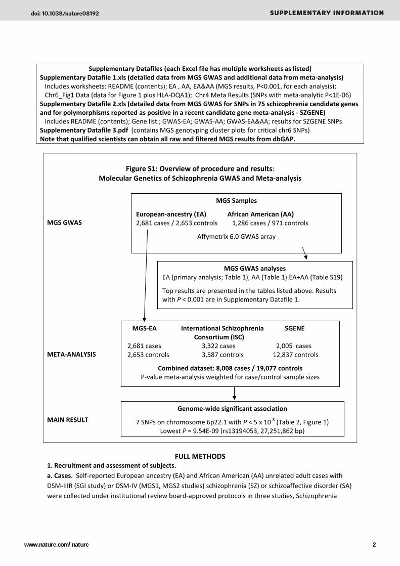
Supplementary Datafiles (each Excel file has multiple worksheets as listed) Supplementary Datafile 1.xls (detailed data from MGS GWAS and additional data from meta‐analysis) Includes worksheets: README (contents); EA , AA, EA&AA (MGS results, P<0.001, for each analysis); Chr6_Fig1 Data (data for Figure 1 plus HLA‐DQA1); Chr4 Meta Results (SNPs with meta‐analytic P<1E‐06) Supplementary Datafile 2.xls (detailed data from MGS GWAS for SNPs in 75 schizophrenia candidate genes and for polymorphisms reported as positive in a recent candidate gene meta‐analysis ‐ SZGENE) Includes README (contents); Gene list ; GWAS‐EA; GWAS‐AA; GWAS‐EA&AA; results for SZGENE SNPs Supplementary Datafile 3.pdf (contains MGS genotyping cluster plots for critical chr6 SNPs) Note that qualified scientists can obtain all raw and filtered MGS results from dbGAP.
Figure S1: Overview of procedure and results: Molecular Genetics of Schizophrenia GWAS and Meta‐analysis
MGS GWAS META‐ANALYSIS
A. Full Methods MAIN RESULT
FULL METHODS
1. Recruitment and assessment of subjects. a. Cases. Self‐reported European ancestry (EA) and African American (AA) unrelated adult cases with DSM‐IIIR (SGI study) or DSM‐IV (MGS1, MGS2 studies) schizophrenia (SZ) or schizoaffective disorder (SA) were collected under institutional review board‐approved protocols in three studies, Schizophrenia
MGS‐EA International Schizophrenia SGENE Consortium (ISC) 2,681 cases 3,322 cases 2,005 cases 2,653 controls 3,587 controls 12,837 controls
Combined dataset: 8,008 cases / 19,077 controls P‐value meta‐analysis weighted for case/control sample sizes
Genome‐wide significant association
7 SNPs on chromosome 6p22.1 with P < 5 x 10‐8 (Table 2, Figure 1) Lowest P = 9.54E‐09 (rs13194053, 27,251,862 bp)
MGS GWAS analyses EA (primary analysis; Table 1), AA (Table 1).EA+AA (Table S19)
Top results are presented in the tables listed above. Results with P < 0.001 are in Supplementary Datafile 1.
MGS Samples
European‐ancestry (EA) African American (AA) 2,681 cases / 2,653 controls 1,286 cases / 971 controls
Affymetrix 6.0 GWAS array
doi: 10.1038/nature08192 SUPPLEMENTARY INFORMATION
www.nature.com/nature 2

Genetics Initiative (SGI)1, Molecular Genetics of Schizophrenia Part 1 (MGS1)2, and MGS23, as previously described in detail in those references. Briefly: SGI subjects (2.4%) were recruited by three research groups in the United States (see Acknowledgments) in a study designed to collect families with affected sibling pairs (and other affected members when available), ascertaining through probands with schizophrenia recruited through clinical settings. One member per family (proband) SGI family was selected for the GWAS sample. MGS1 subjects (10.4%) were collected by ten sites (see acknowledgements) in the United States and Australia in a study designed to collect affected sibling pairs (and other affected members when available), ascertaining through probands with schizophrenia recruited through clinical settings and community residences. One member per MGS1 family (proband) was selected for the GWAS sample. MGS2 (87.2%) subjects were collected by the same ten sites as MGS1. Single cases were selected (and both parents were asked to provide blood samples to collect case‐parent trios where possible, families were not studied in the GWAS except for quality control purposes). Probands had DSM‐IV schizophrenia, or DSM‐IV schizoaffective disorder but with a history of meeting Criteria A for schizophrenia for at least six months of the course of illness. These two disorders co‐aggregate in families with similar relative risks.4
Table S1: Sources of clinical information for MGS subjects
Source of information % of subjects
Number of sources
% of subjects
Family history of psychosis
% of subjects
DIGS 2.0 97.4% 1 1.5% None known 69.3% FIGS 2.0 32.9% 2 68.1% Likely 13.8% Med Records 89.8% 3 30.4% Definite 16.8%
The three studies used the same clinical assessments (with minor modifications for MGS1 and 2 compared with SGI) and diagnostic procedures. Across all cases regardless of study, Table S1 summarizes the sources of information available, as well as the results of screening for family history of psychotic disorders. Interviews were conducted in person by trained research interviewers using the Diagnostic Interview for Genetic Studies v2.0 (DIGS)5; the Family Interview for Genetic Studies (FIGS)5 was completed with an informant where possible; and medical records were obtained with the subject’s written consent. The DIGS versions used in SGI and MGS are available at http://nimhgenetics.org. Almost all cases had at least two sources of information; in the 1.5% of cases where only one source was available, this was medical records in all but two, in situations where the subject was willing to participate and sign consent for the study, but was unable to give reliable historical information (or preferred not to do so), and informants were not available, but there were extensive clinical records that permitted a confident diagnosis.
In all three studies, two expert diagnosticians then independently reviewed all available information about each case, made all applicable diagnoses (DSM‐IIIR for SGI which was completed earlier; DSM‐IV for MGS), and they arrived at a primary consensus best‐estimate final diagnosis6 of SZ or SA for included cases (in MGS2 this required a consensus confidence level of "definite" or "likely"). For MGS1 and 2 (97.6% of cases), the consensus ratings included each DSM schizophrenia criterion, a confidence level for each diagnosis, ratings of family history, and dimensional ratings of symptoms and course.
doi: 10.1038/nature08192 SUPPLEMENTARY INFORMATION
www.nature.com/nature 3

Table S2a: Demographic characteristics and diagnoses MGS cases
Analyzed sample EA cases EA controls AA cases AA controls
Sex Count % count % count % count % Male 1,865 69.9 1,269 47.8 803 62.4 381 39.2 Female 816 30.1 1,384 52.2 483 37.6 592 60.8 2,681 2,653 1286 973
Age Mean SD mean SD mean SD mean SD at evaluation 43.0 11.6 50.6 16.4 42.7 10.4 45.6 13.1 at onset 21.4 7.0 na na 20.9 6.8 na na
Diagnosis Count % count % count % count % SCZ 2,375 88.6 na na 1,173 91.2 na na SADT 120 4.5 na na 58 4.5 na na SAMT 186 6.9 na na 55 4.3 na na
AU CO NUH ATL WU STAN NY LSU UCSF IW SGI 633 500 487 452 396 386 288 284 230 214 97
(AU=Australia; CO=Colorado; NUH=Northshore University Health System; ATL=Emory Univ.; STAN=Stanford; NY=Mt. Sinai; LSU=LSU New Orleans; UCSF=U California San Francisco; IW=Univ Iowa; SGI=NIMH Schizophrenia Genetics Initiative.)
Table S2b: Clinical differences between schizophrenia and schizoaffective cases
SCZ SA SCZ SA P Mean SD Mean SD P % %
AgeRx 22.84 7.55 22.77 7.49 0.86 Sex (female) 30.6 50.8 <1E‐08 AAO 21.21 6.80 21.49 7.89 0.49 “A” criteria‐SCZ (present/absent) PosSx 20.93 3.81 20.60 3.85 0.11 Delusions 98.4 99.5 0.08 BizPosSx 16.03 10.35 16.51 10.24 0.38 Bizarre Delusions 63.3 58.6 0.07 Neg/Disorg 17.82 8.28 15.20 8.49 2E‐08 Hallucinations 94.6 93.7 0.49 MoodSx 5.27 6.06 13.40 6.53 <1E‐08 SCZ hallucinations 50.1 48.4 0.53 Deterioration 3.48 0.81 3.48 0.84 0.97 Disorg Speech 67.9 59.0 3E‐04 SumCritA 5.23 1.34 4.94 1.36 5E‐05 Disorg Behavior 67.6 57.5 4E‐05 Negative Symptoms 83.5 81.2 0.24
AgeRx = age at first treatment for psychosis); AAO = age at onset; SumCritA = sum of schizophrenia “A” criteria (column 2). Symptom factors (M plus) include “PosSx” (positive symptoms; delusions, hallucinations and paranoia), “BizPosSx” (bizarre positive symptoms; control delusions, other bizarre delusions, commenting/conversing hallucinations, thought broadcasting/audible thoughts/thought echo); “Neg/Disorg” (negative and disorganized symptoms; blunted affect, poverty of speech, formal thought disorder, disorganized behavior) and “MoodSx” (mood symptoms; depression, mania, and mood‐congruent psychotic symptoms). Table S2a summarizes demographic, diagnostic and recruitment site information about post‐QC MGS2 cases and controls. Table S2b summarizes contrasts of clinical variables in schizophrenia vs. schizoaffective cases (note that the analyses of symptom factors include 3,552 subjects with valid and complete ratings). Data are final consensus diagnostician ratings based on all sources of information. Analyses were t‐tests for continuous variables (left column) and χ2 for categorical variables (right column. Symptom factors are based on diagnostician ratings of duration and severity using the Lifetime Dimensions of Psychosis Scale (LDPS).7
Family studies consistently demonstrate familial co‐aggregation of schizophrenia and schizoaffective disorder.4,8,9 Diagnostic criteria separating these two disorders are subjective, and inter‐rater reliability is often low across research groups.10 One large family study found the highest familial risk of
doi: 10.1038/nature08192 SUPPLEMENTARY INFORMATION
www.nature.com/nature 4

schizophrenia in relatives of schizophrenia probands with severe, chronic illness and manic features.11 However, because some DSM‐IV schizoaffective patients have only brief periods of persistence of psychosis after long mood disorder episodes, which bears little resemblance to schizophrenia, the MGS investigators decided in advance to include schizoaffective cases, but to require at least six months of illness consistent with schizophrenia (and mood disorder during ≥ 30% of the clinical course).
Table 2b shows that schizoaffective and schizophrenia cases had similar AAO, positive symptoms, bizarre positive symptoms (characteristic of schizophrenia) and deterioration of functioning. Schizophrenia cases had more negative symptoms, disorganized thinking and behavior; schizoaffective cases were more likely to be female. This is indeed one of the problems with this distinction: female patients have on average a later age at onset (P=1E‐04 here for schizophrenia cases); later‐onset cases tend to have greater preservation of affect and communication, which makes it easier for clinicians to obtain descriptions of “mood”symptoms. Note for example that in this sample, the ratio of males to females was 2.27:1, but for both subtypes of schizoaffective disorder (depressed and bipolar types), the ratio was approximately 1:1. There is no evidence from family or twin studies that schizoaffective disorder “breeds true,” and much greater evidence for a genetic relationship to schizophrenia. Here, we achieved our goal of recruiting severely ill schizoaffective cases with illnesses that are clinically consistent with schizophrenia, thereby recruiting the entire range of schizophrenia cases, with and without concurrent mood symptoms. The primary analysis has been carried out based on this a priori ascertainment rule.
b. Controls. EA and AA unrelated adult control subjects were collected under MGS2 as previously described3 by Knowledge Networks (Menlo Park, CA). Briefly, KN uses random digit dialing to area codes selected to represent the national population, to recruit individuals to join a nationwide survey panel (approximately 60,000 individuals at any one time, with constant turnover). Communication with panel members is by email and web interaction, but initial recruitment does not require internet connection, and those who agree to join but have no internet access are given a web TV to facilitate participation. Panel members are then contacted to invite participation in specific surveys. All EA control subjects and 41% of AA controls were recruited by KN using these methods. There was an insufficient number of AA individuals in the panel who were interested in participating to complete the collection, thus KN contracted with a second survey research company (SSI Opt‐In). SSI/Opt‐in uses banner ads on websites to recruit participants. In total, 3,364 EA and 1,301 AA control subjects were recruited, of which 772 AA subjects (59%) were recruited by SSI/Opt‐in. KN recruited a control subject from 21.7% of targeted EA and 15.7% of targeted AA households consented, completed the clinical questionnaire and provided a blood specimen, which is a high rate for population‐based studies requiring a blood sample. SSI/Opt‐ completed only 2.1% of targeted individuals (i.e., who initially responded to ads). Table S3 compares demographic characteristics of individuals targeted for recruitment by KN vs. the final sample. There is an excellent match except for an upward shift in education which is larger for AA than for EA subjects. Using an IRB‐approved procedure, individuals who responded to the initial invitation to participate were provided with an explanation of the study online (with an opportunity to phone for more information), and provided preliminary consent online. Participation required completion of an online clinical questionnaire. For those who completed the questionnaire, a national phlebotomy company (EMSI)
doi: 10.1038/nature08192 SUPPLEMENTARY INFORMATION
www.nature.com/nature 5
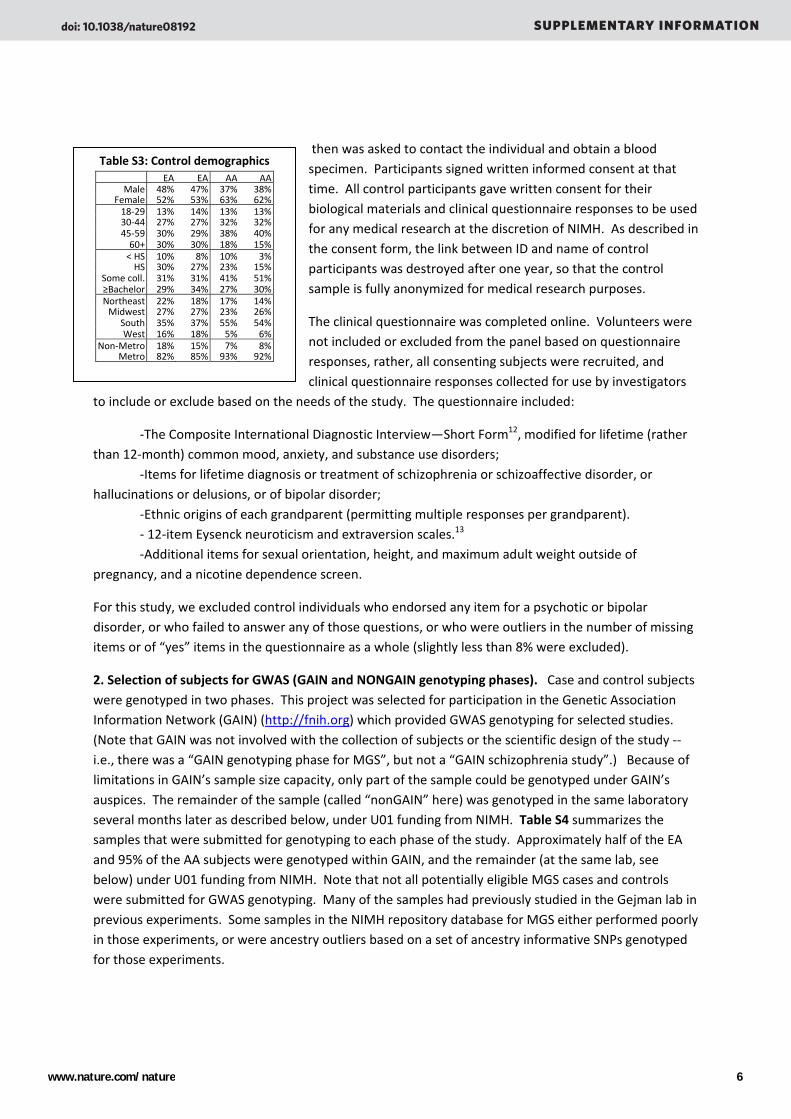
Table S3: Control demographics EA EA AA AA
Male 48% 47% 37% 38% Female 52% 53% 63% 62% 18‐29 13% 14% 13% 13% 30‐44 27% 27% 32% 32% 45‐59 30% 29% 38% 40% 60+ 30% 30% 18% 15% < HS 10% 8% 10% 3% HS 30% 27% 23% 15%
Some coll. 31% 31% 41% 51% ≥Bachelor 29% 34% 27% 30% Northeast 22% 18% 17% 14% Midwest 27% 27% 23% 26%
South 35% 37% 55% 54% West 16% 18% 5% 6%
Non‐Metro 18% 15% 7% 8% Metro 82% 85% 93% 92%
then was asked to contact the individual and obtain a blood specimen. Participants signed written informed consent at that time. All control participants gave written consent for their biological materials and clinical questionnaire responses to be used for any medical research at the discretion of NIMH. As described in the consent form, the link between ID and name of control participants was destroyed after one year, so that the control sample is fully anonymized for medical research purposes.
The clinical questionnaire was completed online. Volunteers were not included or excluded from the panel based on questionnaire responses, rather, all consenting subjects were recruited, and clinical questionnaire responses collected for use by investigators
to include or exclude based on the needs of the study. The questionnaire included:
‐The Composite International Diagnostic Interview—Short Form12, modified for lifetime (rather than 12‐month) common mood, anxiety, and substance use disorders; ‐Items for lifetime diagnosis or treatment of schizophrenia or schizoaffective disorder, or hallucinations or delusions, or of bipolar disorder; ‐Ethnic origins of each grandparent (permitting multiple responses per grandparent). ‐ 12‐item Eysenck neuroticism and extraversion scales.13 ‐Additional items for sexual orientation, height, and maximum adult weight outside of pregnancy, and a nicotine dependence screen.
For this study, we excluded control individuals who endorsed any item for a psychotic or bipolar disorder, or who failed to answer any of those questions, or who were outliers in the number of missing items or of “yes” items in the questionnaire as a whole (slightly less than 8% were excluded).
2. Selection of subjects for GWAS (GAIN and NONGAIN genotyping phases). Case and control subjects were genotyped in two phases. This project was selected for participation in the Genetic Association Information Network (GAIN) (http://fnih.org) which provided GWAS genotyping for selected studies. (Note that GAIN was not involved with the collection of subjects or the scientific design of the study ‐‐ i.e., there was a “GAIN genotyping phase for MGS”, but not a “GAIN schizophrenia study”.) Because of limitations in GAIN’s sample size capacity, only part of the sample could be genotyped under GAIN’s auspices. The remainder of the sample (called “nonGAIN” here) was genotyped in the same laboratory several months later as described below, under U01 funding from NIMH. Table S4 summarizes the samples that were submitted for genotyping to each phase of the study. Approximately half of the EA and 95% of the AA subjects were genotyped within GAIN, and the remainder (at the same lab, see below) under U01 funding from NIMH. Note that not all potentially eligible MGS cases and controls were submitted for GWAS genotyping. Many of the samples had previously studied in the Gejman lab in previous experiments. Some samples in the NIMH repository database for MGS either performed poorly in those experiments, or were ancestry outliers based on a set of ancestry informative SNPs genotyped for those experiments.
doi: 10.1038/nature08192 SUPPLEMENTARY INFORMATION
www.nature.com/nature 6

Table S4: Summary of genotyped MGS samples
European ancestry subjects African American subjects case control Duplicate Trio Case Control duplicate trio GAIN 1404 1442 29 31 1257 990 23 18 NonGAIN 1434 1375 32 31 101 20 8 2 Total 2838 2817 61 62 1358 1010 31 20
Note: The same 31 EA trios (probands and their parents) were genotyped in GAIN and in NonGAIN.
3. Genotyping. Genotyping was carried out at the Broad Institute National Center for Genotyping and Analysis (funded by the U.S. National Center for Research Resources), under the directions of Drs. Stacey Gabriel and Daniel Mirel. (Note that the GAIN genotyping was carried in this lab in the Fall of 2007, and the nonGAIN genotyping in the Spring of 2008, using the same chip and procedures.) Genotyping was carried using the Affymetrix 6.0 array, which assays 906,600 SNPs and 946,000 “copy number probes” (for non‐polymorphic sites for analysis of copy number in gaps between SNPs.14
Whereas on the older Affymetrix 500K array “perfect match” and “mismatch” probes for each SNP were tiled onto the array, on the 6.0 array, identical “optimal” PM probes are tiled for each allele. Genotype calls were made the BIRDSEED program, a module of the BIRDSUITE package.15 A summary of QC parameter values for the final, post‐QC dataset is shown Table S5, and details are provided below. Genotypes are called based on normalized intensity values for the colors labeling the two alleles. BIRDSEED sets expected locations for the three genotype cluster centers for each SNP, based on HapMap sample data, and then searches for the true centers. Because these centers can shift in different genotyping runs, calls are usually made on batches of arrays run at approximately the same time (e.g., a 96‐well plate), which maximizes call rate (as we confirmed with our own data). Genotypes with confidence > 0.1 score (as defined by Korn et al.) were considered “missing.”
4. Quality control of genotype data. QC of the GAIN EA and AA datasets was carried out in close collaboration with Justin Paschall of NCBI in collaboration with the GAIN analysis consultant, Dr. Gonçalo Abecasis (University of Michigan). One of the benefits of the GAIN project was the opportunity that it provided for investigators to learn from each other about GWAS analysis issues. We are indebted to these individual for their contributions to the QC of our data. Quality control and association analyses were carried out with the software package PLINK16, supplemented where needed by custom scripts and programs.
4a. Exclusion criteria for DNA samples ‐ European ancestry (EA) subjects. EA subjects were excluded if they had:
(1) genotyping call rate less than 97%;
(2) genotypic gender inconsistent with the gender reported by the site or control data file;
Table S5: Genotyping QC (final dataset)
Post‐QC dataset EA AA Samples ‐ Total N: 5334 2259 Avg Call Rate 99.7% 99.6% SNPs ‐ Total N: 696,788 843,468 Call Rate ‐ Autosomes 99.7% 99.6% ‐ X 99.8% 99.5% Dup. concordance ‐ Aut 99.8% 99.7% ‐ X 99.8% 99.85%
doi: 10.1038/nature08192 SUPPLEMENTARY INFORMATION
www.nature.com/nature 7

(3) a proportion of heterozygous genotypes > 28.5% or < 26.0%. Unusually high or low heterozygosity values are thought to occur primarily because of genotyping/DNA quality problems (or ancestry differences as discussed below). Note that these thresholds were based on analyses using all SNPs for which data were reported by the lab, prior to other QC. The appropriate threshold will vary according to the range of minor allele frequencies in the data (which also varies with ancestry).
(4) one or more ancestry‐related principal component scores (see below) that were considered outliers to the distribution of that score, indicating greater African, Asian or Native American ancestry.
For each pair of genotyped duplicates, one sample was excluded if it was a heterozygosity outlier or had a lower genotyping call rate.
We performed IBD analysis to confirm known family relationships and to detect unexpected (“cryptic,” unsuspected) relationships. Genome‐wide kinship was estimated for each pair of subjects based on the IBS of 167,302 SNPs (one from each consecutive four post‐QC SNPs as described below). Eighteen subjects were excluded because they had estimated kinship coefficients larger than 0.1 with at least 50 other subjects. Six unexpected duplicates, nineteen unexpected parent‐child pairs, three unexpected sibling pairs and two unexpected grandparent‐child pairs were detected according to the IBD sharing pattern. For each relative pair, we excluded the subject with lower genotyping call rate or extreme heterozygosity proportion. When two related controls had similar QC metrics, we excluded the younger control subject (because the subject had passed through less of the period of risk for schizophrenia). When two related cases had similar QC metrics, we examined the clinical data (blind to genotype or association results) and chose the case with the best documentation of clinical features. For the six cryptic duplicate pairs, we excluded one subject of lower call rate from four pairs and excluded both subjects for the other two pairs because the DNA identification/contamination.
Table S6 summarizes how many EA subjects were excluded by each criterion (some failed multiple criteria); 321 cases/controls were excluded from the 5,655 submitted for genotyping (5.68%).
Table S6: Number of subjects excluded by QC filters for autosomal SNP analysis
Criterion European ancestry African American call rate 119 36 heterozygosity proportion 168 19 inconsistent gender 31 18 unexpected duplicate 81 1 unexpected relatedness 23 0 principal component outliers 28 18 subjects with kinship > 0.1 with more than 50 subjects 18 3 clinical data review 2 2 Total subjects excluded 321 109
Note: 1Among six cryptic duplicate pairs, both subjects excluded for 2 pairs and one subject excluded for 4 pairs.
For the EA subjects passing sample QC criteria, we performed additional QC for X‐chromosome analysis. Because males always have homozygous genotypes while females may have three possible genotypes, males have higher call rates than females. We excluded any male subject if his X chromosome call rate was less than 98.8% (based on the observed distribution of male genotyping call rate). We excluded any female if the X chromosome call rate was less than 97.0%, or if the X chromosome proportion of
doi: 10.1038/nature08192 SUPPLEMENTARY INFORMATION
www.nature.com/nature 8
heterozygous SNPs was larger than 40% or less than 24% (thresholds chosen based on observed distributions). In total, sixty‐five additional EA subjects were excluded for X chromosome SNP association analysis (Table S7).
Table S7: Number of additional EA subjects excluded by QC filters for X‐chr analysis only
Criterion European ancestry African American call rate male 11 2 call rate female 50 0 heterozygosity proportion female 4 0 Total subjects excluded 65 2
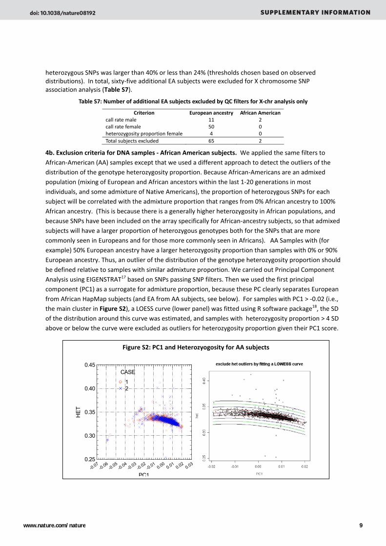
4b. Exclusion criteria for DNA samples ‐ African American subjects. We applied the same filters to African‐American (AA) samples except that we used a different approach to detect the outliers of the distribution of the genotype heterozygosity proportion. Because African‐Americans are an admixed population (mixing of European and African ancestors within the last 1‐20 generations in most individuals, and some admixture of Native Americans), the proportion of heterozygous SNPs for each subject will be correlated with the admixture proportion that ranges from 0% African ancestry to 100% African ancestry. (This is because there is a generally higher heterozygosity in African populations, and because SNPs have been included on the array specifically for African‐ancestry subjects, so that admixed subjects will have a larger proportion of heterozygous genotypes both for the SNPs that are more commonly seen in Europeans and for those more commonly seen in Africans). AA Samples with (for example) 50% European ancestry have a larger heterozygosity proportion than samples with 0% or 90% European ancestry. Thus, an outlier of the distribution of the genotype heterozygosity proportion should be defined relative to samples with similar admixture proportion. We carried out Principal Component Analysis using EIGENSTRAT17 based on SNPs passing SNP filters. Then we used the first principal component (PC1) as a surrogate for admixture proportion, because these PC clearly separates European from African HapMap subjects (and EA from AA subjects, see below). For samples with PC1 > ‐0.02 (i.e., the main cluster in Figure S2), a LOESS curve (lower panel) was fitted using R software package18, the SD of the distribution around this curve was estimated, and samples with heterozygosity proportion > 4 SD above or below the curve were excluded as outliers for heterozygosity proportion given their PC1 score.
Figure S2: PC1 and Heterozyogosity for AA subjects
-0.07-0.06
-0.05-0.04
-0.03-0.02
-0.010.00
0.010.02
0.03
PC1
0.25
0.30
0.35
0.40
0.45
HET
21
CASE
doi: 10.1038/nature08192 SUPPLEMENTARY INFORMATION
www.nature.com/nature 9
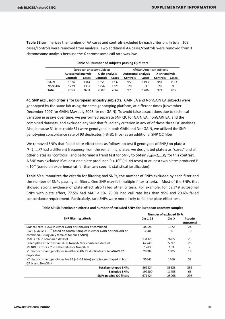
Table S8 summarizes the number of AA cases and controls excluded by each criterion. In total, 109 cases/controls were removed from analysis. Two additional AA cases/controls were removed from X chromosome analysis because the X chromosome call rate was low.
Table S8: Number of subjects passing QC filters
European ancestry subjects African American subjects Autosomal analysis X‐chr analysis Autosomal analysis X‐chr analysis Controls Cases Controls Cases Controls Cases Controls Cases GAIN 1374 1344 1351 1337 953 1193 951 1193 NonGAIN 1279 1337 1256 1325 20 93 20 93 Total 2653 2681 2607 2662 973 1286 971 1286
4c. SNP exclusion criteria for European ancestry subjects. GAIN EA and NonGAIN EA subjects were genotyped by the same lab using the same genotyping platform, at different times (November‐December 2007 for GAIN; May‐July 2008 for nonGAIN). To avoid false associations due to technical variation in assays over time, we performed separate SNP QC for GAIN EA, nonGAIN EA, and the combined datasets, and excluded any SNP that failed any criterion in any of of these three QC analyses. Also, because 31 trios (table S1) were genotyped in both GAIN and NonGAIN, we utilized the SNP genotyping concordance rate of 93 duplicates (=3×31 trios) as an additional SNP QC filter.
We removed SNPs that failed plate effect tests as follows: to test if genotypes of SNP j on plate k (k=1,…,K) had a different frequency from the remaining plates, we designated plate k as “cases” and all other plates as “controls”, and performed a trend test for SNP j to obtain Pjk(k=1,…,K)
for this contrast. A SNP was excluded if at least one plate produced P < 10‐8 (~1 /N tests) or at least two plates produced P < 10‐4 (based on experience rather than any specific statistical justification).
Table S9 summarizes the criteria for filtering bad SNPs, the number of SNPs excluded by each filter and the number of SNPs passing all filters. One SNP may fail multiple filter criteria. Most of the SNPs that showed strong evidence of plate effect also failed other criteria. For example, for 62,749 autosomal SNPs with plate effect, 77.5% had MAF < 1%, 25.0% had call rate less than 95% and 20.6% failed concordance requirement. Particularly, rare SNPs were more likely to fail the plate effect test.
Table S9: SNP exclusion criteria and number of excluded SNPs for European ancestry samples
Number of excluded SNPs SNP filtering criteria Chr 1‐22 Chr‐X Pseudo
autosomal SNP call rate < 95% in either GAIN or NonGAIN or combined 44624 1872 24 HWE p‐value < 10‐6 based on control samples in either GAIN or NonGAIN or combined, (using only females for chr X SNPs)
3840 86 10
MAF < 1% in combined dataset 134325 9265 25 Failed plate effect test in GAIN, NonGAIN or combined dataset 62749 5097 26 MENDEL errors > 2 in either GAIN or NonGAIN 1783 163 2 >1 disconcordant genotypes in either GAIN 29 duplicates or NonGAIN 32 duplicates
29582 1005 19
>2 disconcordant genotypes for 93 (=3×31 trios) samples genotyped in both GAIN and NonGAIN
36543 1466 32
Total genotyped SNPs 869224 36523 362 Excluded SNPs 197800 11455 66
SNPs passing QC filters 671424 25068 296
doi: 10.1038/nature08192 SUPPLEMENTARY INFORMATION
www.nature.com/nature 10
4d. SNP exclusion criteria for African American subjects. Because there were only 102 cases and 20 controls in the NonGAIN AA dataset, compared with 1256 cases and 990 controls in the GAIN AA data, we performed SNP QC by combining all AA subjects. The SNP QC metrics were computed based on subjects passing sample QC criteria. Table S10 summarizes the criteria for excluding SNPs, the number of SNPs excluded by each filter and the number of SNPs passing all filters. Note that there were only 16,824 autosomal SNPs with MAF < 1% in African American samples compared to 134,325 in European ancestry samples. This difference also explained the fact that the number of SNPs with evidence of plate effect in African American sample was much less than that in European ancestry samples because rare SNPs were more likely to fail plate effect test.
Table S10: SNP exclusion criteria for African American samples
Number of excluded SNPs SNP filtering criteria Chr 1‐22 Chr‐X Pseudo autosomal
call rate < 95% 30179 1514 18 HWE p‐value < 10‐6 2248 69 3 MAF < 1% 16824 1942 10 failed plate effect test 7814 571 7 MENDEL errors > 2 968 95 1 disconcordant genotypes > 1 15661 549 11
Total genotyped SNPs 869224 36523 362 Excluded SNPs 57884 4395 32
SNPs passing QC filters 811340 32128 330
5. Analysis of population substructure . Principal Components Analyses were carried out with
EIGENSTRAT17 to evaluate population substructure and to determine optimal corrections. Data for one out of every four SNPs (as described above) were included and PC scores included for each subject (typically 20 scores). It has been previously shown that some of these will reflect ancestry differences among subjects, as indexed by allele frequency differences among the ancestral populations that are represented. Two main types of ancestral variation are of interest here: the major continental
ancestries (European, African and Asian ‐‐ with Native American resembling Asian at this scale); and within‐Europe variation. In order to understand the within‐Europe ancestries that are indexed by different PCs, we select ~ 1840 MGS cases and controls who reported a single ancestry on both sides of their families (with no ancestry reported as “don’t know”) ‐‐ these data were collected in both the DIGS interview for cases and in the clinical questionnaire administered to controls. These relationships are summarized below.
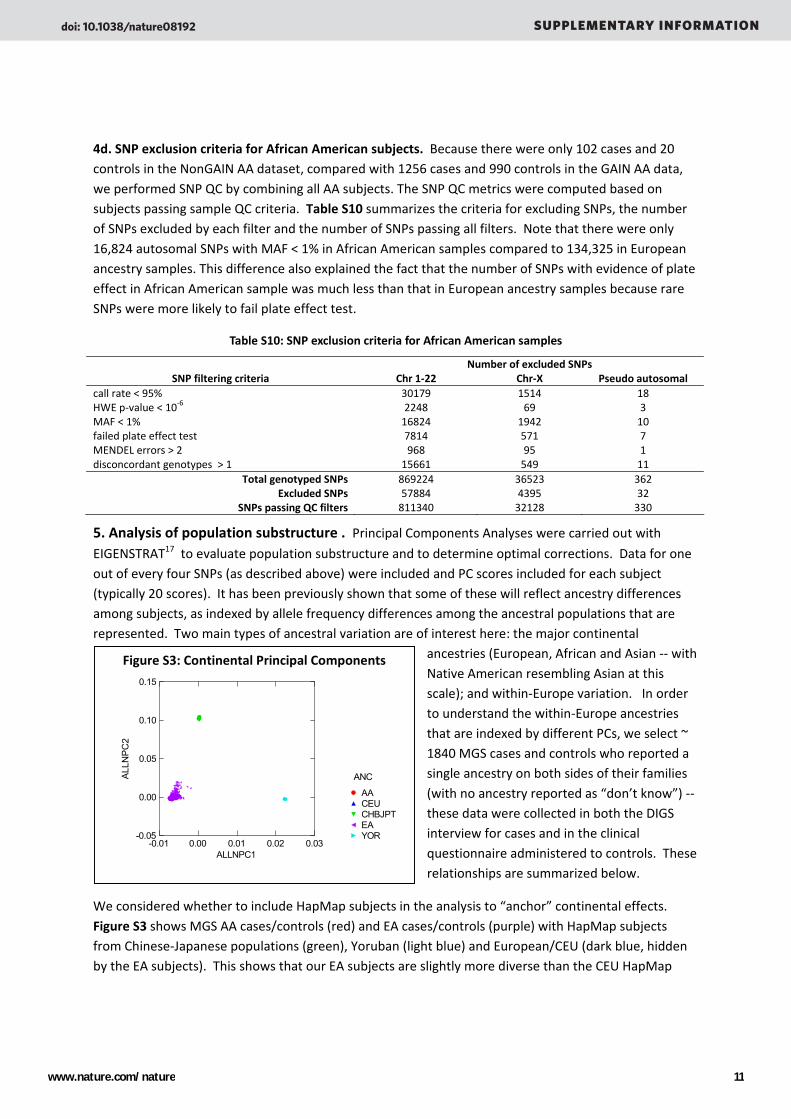
We considered whether to include HapMap subjects in the analysis to “anchor” continental effects. Figure S3 shows MGS AA cases/controls (red) and EA cases/controls (purple) with HapMap subjects from Chinese‐Japanese populations (green), Yoruban (light blue) and European/CEU (dark blue, hidden by the EA subjects). This shows that our EA subjects are slightly more diverse than the CEU HapMap
Figure S3: Continental Principal Components
-0.01 0.00 0.01 0.02 0.03ALLNPC1
-0.05
0.00
0.05
0.10
0.15
ALL
NP
C2
YOREACHBJPTCEUAA
ANC
doi: 10.1038/nature08192 SUPPLEMENTARY INFORMATION
www.nature.com/nature 11

subjects, with one projection toward the Asian pole (probably due to small Native American admixtures in some subjects), and one toward the African pole (which we show below is due to Mediterranean and Askhkenazi Jewish ancestry). The AA subjects have highly variablle degrees of European admixture.
However, one captures these variations with or without HapMap subjects in the PCA. Table S11 shows correlations of EAPCs (PCs for EA cases/controls without HapMap subjects) vs. ALLPCs (computed with EA, AA and HapMap subjects). The major PCs that were detected in the analysis with HapMap subjects included were also detected in the analysis that included only the EA subjects. Note that in this table, we have indicated which PCs show a geographical gradient, based on the analyses discussed below. “N‐S” indicates North‐South, “E‐W” is East‐West, “Ashk” is Ashkenazi. Another effect illustrated here is that when SNPs throughout the genome are included in the analysis, there are components which are entirely due to local effects. For example, in Table S10, EAPC3 and ALLPC4 are due almost entirely to variation within the chromosome 8p common inversion region (~ 8‐12 Mb), and to variation within the chromosome 6 MHC region (~ 24‐35 Mb), as well as several smaller contributions from other regions.
Table S11: Correlation of EA PCs computed with (ALLPCs) vs. without (EAPCs) HapMap subjects
Geog EAPCs→ 1 2 3 4 5 6 7 8 9 10 ALLPCs↓ N‐S 1 0.844 ‐0.159 0.027 ‐0.021 ‐0.145 0.115 ‐0.002 0.005 0.017 ‐0.014 N‐S 2 0.398 ‐0.455 0.056 0.185 ‐0.370 0.048 ‐0.014 ‐0.101 ‐0.034 ‐0.056 N‐S 3 0.992 0.349 ‐0.011 ‐0.024 0.140 0.172 0.076 0.050 0.037 0.067 (8p) 4 ‐0.007 ‐0.243 ‐0.943 0.364 ‐0.223 0.112 ‐0.048 ‐0.075 ‐0.078 ‐0.026 E‐W 5 ‐0.014 ‐0.148 0.245 0.917 0.102 ‐0.056 0.023 ‐0.042 ‐0.028 0.027 none 6 0.067 ‐0.412 0.097 ‐0.267 0.655 0.335 0.158 0.106 ‐0.079 0.065 Ashk 7 ‐0.064 ‐0.071 0.035 0.072 ‐0.096 ‐0.641 0.637 ‐0.172 ‐0.166 0.120 Ashk 8 ‐0.099 ‐0.040 ‐0.021 ‐0.022 0.161 ‐0.580 ‐0.670 0.054 0.177 0.080 none 9 ‐0.075 0.054 ‐0.019 ‐0.031 0.244 ‐0.310 ‐0.050 ‐0.579 0.273 ‐0.469 none 10 ‐0.018 0.050 ‐0.018 ‐0.066 0.065 ‐0.116 0.193 0.611 0.299 ‐0.629
Geog N‐S sl N‐S (8p) E‐W none Ashk/MHC
Ashk/MHC
none none none
Figure S4: Correlations of EA PCs with SNPs in chromosomes 8p (left) and 6p (right)
doi: 10.1038/nature08192 SUPPLEMENTARY INFORMATION
www.nature.com/nature 12

These local effects can be demonstrated by computing the linear correlation between SNP genotypes (coded as the number of one of the alleles present in each subject, 0‐2) and each PC score. Alternatively, in PLINK one can simply perform a quantitative association analysis for each PC score for
the SNPs included in the PCA (S. Purcell, personal communication). Figure S4 illustrates a genome‐wide “Manhattan” plot where each dot is the Pearson correlation (varying above and below 0 in the middle of the Y axis) between genotypes for one SNP and the PC score being tested. The left plot shows that EAPC 3 is driven almost entirely by SNPs from the 8p inversion, and the right plot shows that EAPC6 is driven by a combination of SNPs throughout the genome and, more strongly, by SNPs on chromosome 6p which are within the MHC region. Figure S5 shows that EAPC3 (chr 8p), on the Y‐axis, produces a characteristic pattern of 3 clusters which do not correlate
with geographical ancestry ‐‐ in our experience, 8p always produced one of the larger PCs in European‐ancestry data, and always produces this pattern. Consistent with approaches suggested by others (G. Abecasis, personal communication to DFL; N. Patterson, personal communication to DFL), we were concerned about obscuring evidence for association in a local region by correcting association tests for a PC reflecting variation only in that region. This might be particularly true for MHC‐associated diseases.
Therefore, we removed chr8:8‐12Mb and Chr6:24‐35Mb SNPs and re‐computed all PCs, now designated as EANPCs (MGS EA subjects only, no chr6 or chr8), AANPCs (AA subjects only) and ALLPCs (EA and AA subjects plus HapMap subjects).
Table S12 shows correlations between EANPCs and ALLNPCs, and again, both continental and within‐Europe dimensions are detected either way, with a high correlation between specific pairs of components. Also shown are the P‐values for t‐tests for EA case vs. control values for each PC.
Table S12: Correlation (EA subjects): NPCs with (ALLNPCs) vs. without (EANPCs) HapMap subjects
Case‐cont P Geog EANPCs→ 1 2 3 4 5 6 7 8 9 10
ALLNPCs↓
1E‐7 N‐S 1 0.842 ‐0.165 ‐0.007 ‐0.168 0.092 0.005 0.009 0.034 ‐0.010 ‐0.0141E‐7 sl N‐S 2 0.399 ‐0.456 ‐0.219 ‐0.337 0.010 ‐0.021 0.061 ‐0.076 ‐0.027 ‐0.0561E‐5 N‐S 3 0.992 0.356 0.024 0.108 0.209 0.009 ‐0.021 0.121 0.003 0.0673E‐3 E‐W 4 ‐0.008 ‐0.148 ‐0.979 0.203 ‐0.058 0.000 0.019 ‐0.049 ‐0.004 ‐0.0260.18 None 5 0.058 ‐0.474 0.176 0.598 0.431 ‐0.018 ‐0.127 0.039 ‐0.003 0.0270.40 Ashk 6 0.116 0.051 ‐0.026 ‐0.223 0.842 0.150 ‐0.097 ‐0.221 0.166 0.0650.19 None 7 0.087 ‐0.063 ‐0.025 ‐0.279 0.234 0.219 ‐0.593 0.311 ‐0.440 0.1200.73 None 8 ‐0.066 0.041 ‐0.006 0.234 ‐0.113 0.768 0.172 ‐0.494 ‐0.002 0.0800.25 None 9 0.039 ‐0.031 0.051 ‐0.150 ‐0.123 0.647 ‐0.056 0.658 0.151 ‐0.4690.69 None 10 ‐0.034 0.011 0.039 ‐0.006 ‐0.184 ‐0.044 ‐0.598 ‐0.152 0.699 ‐0.629
Geography N‐S sl N‐S E‐W None Ashk None None sl. Ashk None None Case‐Cont P 2XE‐7 0.09 0.03 9E‐5 0.32 0.31 0.48 0.93 0.39 0.08
Figure S5: Chr 8p‐specific PC3
-0.015-0.010
-0.0050.000
0.0050.010
0.015
EAPC1
-0.030
-0.015
0.000
0.015
0.030
EAP
C3
21
CASE
doi: 10.1038/nature08192 SUPPLEMENTARY INFORMATION
www.nature.com/nature 13

Table S13 shows similar data for AA subjects, showing that AA subjects show primarily North‐South variation (as expected), indexed by AANPCs 1 and 2, and almost entirely by ALLNPC 1.
Table S13: Correlation (AA subjects): NPCs with (ALLNPCs) vs. without (EANPCs) HapMap subjects
AANPCs→ 1 2 3 4 5 6 7 8 9 10
Case‐Cont P ALLPCs↓ 0.001 1 ‐0.999 ‐0.982 0.009 0.015 0.005 0.005 ‐0.056 ‐0.012 0.060 ‐0.0240.710 2 0.252 0.027 ‐0.001 ‐0.014 ‐0.010 ‐0.010 0.025 ‐0.030 ‐0.022 0.046
0.0001 3 0.166 0.150 0.015 ‐0.008 0.077 ‐0.038 0.037 0.081 ‐0.025 0.0380.064 4 ‐0.151 ‐0.148 0.094 0.042 ‐0.074 ‐0.037 0.003 ‐0.142 0.030 ‐0.0200.780 5 ‐0.001 ‐0.016 0.068 0.026 ‐0.011 ‐0.065 0.025 ‐0.004 0.021 0.0570.250 6 0.022 0.021 0.671 ‐0.013 0.097 0.030 0.099 ‐0.021 ‐0.057 0.0080.340 7 0.004 0.005 ‐0.871 0.108 0.032 0.054 ‐0.125 0.007 0.049 ‐0.0250.050 8 ‐0.002 ‐0.004 ‐0.722 ‐0.121 ‐0.180 ‐0.032 0.044 ‐0.053 0.036 0.0170.051 9 ‐0.010 ‐0.017 0.857 0.109 0.067 0.179 0.052 0.029 ‐0.043 ‐0.0100.390 10 ‐0.004 ‐0.001 ‐0.285 ‐0.306 ‐0.110 0.048 0.019 0.011 ‐0.043 ‐0.004
Case‐Cont P 0.001 0.001 0.140 0.440 0.380 0.320 0.003 0.510 0.500 0.560
Based on these data, we corrected all association tests for PCs computed with the subjects who were actually included in the analysis, but only for PCs that demonstrated either a geographical gradient, and/or which demonstrated a case‐control difference. The selected components are listed in the section on Statistical analysis of association, and the use of these components in the tests is described there. (Note that for AANPCs, we did not correct for AANPC7 which produced a small case‐control difference, because the Eigenvalue for this component is very small and not localized in the genome.
In the course of these analyses, we also observed that there was a modest correlation between PCs computed with autosomal SNPs vs. those computed with chromosome X SNPs. This could reflect differences in the ancestral history of X chromosome SNPs based on very recent ancestry of father and
mother. Therefore, we computed PCs separately for the X chromosome (EAXPCs, AAXPCs, ALLXPCs) and considered their geographical gradients and case‐control differences as for autosomal PCs, selecting appropriate XPCs to correct in analyses (see below).
The relationships of PCs to geographical gradients were determined by plotting pairs of PCs forsubjects who reported a single family ancestry , labeling each ancestry. ANOVAs were carried out in preliminary analyses to confirm relationships. As shown in Figure S6, subjects (cases or controls) who reported one ancestry
are shown by specific symbols (Anglo‐Saxon, Mediterranean, Ashkenazi, Russian/Slavic, Northern European (Scandinavian) and Western European (French, German, etc.); all other cases and controls are
Figure S6: North‐South and East‐West within‐Europe gradients
doi: 10.1038/nature08192 SUPPLEMENTARY INFORMATION
www.nature.com/nature 14

shown in red or blue respectively. PC1 indexes a North‐South gradient, with Anglo‐Saxon and Northern European at the top, then Mediterranean, and then Ashkenazi. Figure S3 (above) shows that African ancestry is far below Ashkenazi. PC3 indexes East‐West, with Russian/Slavic to the right here. Note that case interviews queried childhood religion, so we could distinguish Jews who self‐reported as Russian or Polish (countries of origin for most U.S. Ashkenazi immigrants ) non‐Jewish Slavic families. In the Figure, symbols for Slavic/Russian ancestry appear in both the “Slavic” and the “Ashkenazi” circle, but the latter are Ashkenazi individuals. EANPC5 (=ALLNPC6) further separates the Ashkenazi cluster from all others (Figure S7). Not all PCs with a
geographical distribution differed between cases and controls, but it seemed prudent to include all “geographic” PCs as covariates. Finally, Figure S8 shows that the within‐Europe origins of Australians is similar to that in Americans, except that there are far fewer Ashkenazi individuals in Australia.
6. Statistical analysis of association. Logistic regression analysis was carried out to evaluate the evidence of association for each single marker, correcting for potential population stratification using principal component scores that (1) reflected the population substructure consistent with self‐reported ancestry; or (2) have statistically significant differences between cases and controls; or (3) corresponded to a statistically significant eigenvalue. (Also, the scores were computed without SNPs in the MHC and 8p inversion regions as discussed above.) For X chromosome SNPs, the homozygous genotypes were coded as 0 and 2 for male. For X chromosome SNPs and pseudo autosomal SNPs, we also corrected for sex indicator to eliminate potential bias due to different genotype distribution and strong call rate difference between males and females. Top EA and AA results are shown and discussed in the main text; EA+AA results are shown below in Supplementary Results 1b. The covariates used in the logistic regression models for association analysis were:
EA analyses: EANPCs 1‐5; EAXPCs 1 and 5 (and a covariate for sex) AA analyses: AANPCs 1‐2; AAXPCs 1‐2 (and a covariate for sex) Combined EA+AA analyses (Suppl Results 1b): ALLNPCs 1, 2, 3, 4, 6; ALLXPCs 1,2,5 (and sex)
In response to a reviewer comment about the possibility of unique population structure in the MHC region, we computed principal components (using EIGENSTRAT) using 416 SNPs (out of 2357 post‐QC
Figure S7: EANPC5 separates Ashkenazi ancestry
-0.05 0.00 0.05 0.10EANPC1
-0.020
-0.005
0.010
0.025
0.040
EAN
P C5
WestEurNorthEurRuss/SlavAshkMeditAngloSax
EURANC
Figure S8: US EAs vs. Australians
-0.07-0.06
-0.05-0.04
-0.03-0.02
-0.010.00
0.010.02
0.03
EAPC2
-0.02
-0.01
0.00
0.01
0.02
0.03
0.04
0.05
0.06
0.07
EA
PC
1
USAU
COUNTRY
doi: 10.1038/nature08192 SUPPLEMENTARY INFORMATION
www.nature.com/nature 15
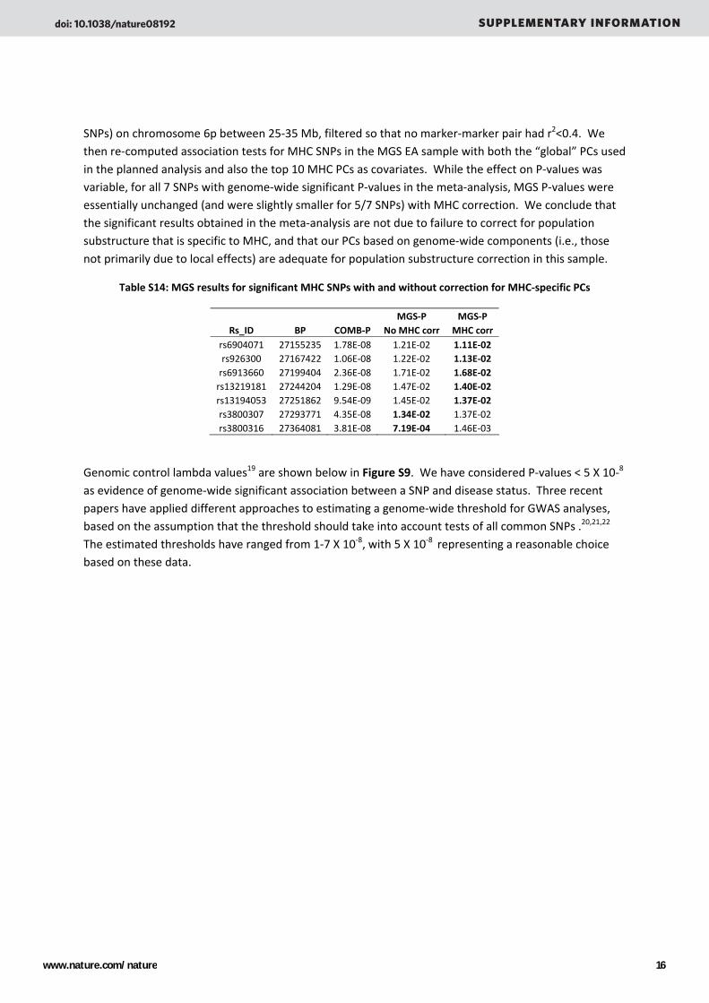
SNPs) on chromosome 6p between 25‐35 Mb, filtered so that no marker‐marker pair had r2<0.4. We then re‐computed association tests for MHC SNPs in the MGS EA sample with both the “global” PCs used in the planned analysis and also the top 10 MHC PCs as covariates. While the effect on P‐values was variable, for all 7 SNPs with genome‐wide significant P‐values in the meta‐analysis, MGS P‐values were essentially unchanged (and were slightly smaller for 5/7 SNPs) with MHC correction. We conclude that the significant results obtained in the meta‐analysis are not due to failure to correct for population substructure that is specific to MHC, and that our PCs based on genome‐wide components (i.e., those not primarily due to local effects) are adequate for population substructure correction in this sample.
Table S14: MGS results for significant MHC SNPs with and without correction for MHC‐specific PCs
MGS‐P MGS‐P Rs_ID BP COMB‐P No MHC corr MHC corr
rs6904071 27155235 1.78E‐08 1.21E‐02 1.11E‐02 rs926300 27167422 1.06E‐08 1.22E‐02 1.13E‐02 rs6913660 27199404 2.36E‐08 1.71E‐02 1.68E‐02 rs13219181 27244204 1.29E‐08 1.47E‐02 1.40E‐02 rs13194053 27251862 9.54E‐09 1.45E‐02 1.37E‐02 rs3800307 27293771 4.35E‐08 1.34E‐02 1.37E‐02 rs3800316 27364081 3.81E‐08 7.19E‐04 1.46E‐03
Genomic control lambda values19 are shown below in Figure S9. We have considered P‐values < 5 X 10‐8 as evidence of genome‐wide significant association between a SNP and disease status. Three recent papers have applied different approaches to estimating a genome‐wide threshold for GWAS analyses, based on the assumption that the threshold should take into account tests of all common SNPs .20,21,22 The estimated thresholds have ranged from 1‐7 X 10‐8, with 5 X 10‐8 representing a reasonable choice based on these data.
doi: 10.1038/nature08192 SUPPLEMENTARY INFORMATION
www.nature.com/nature 16
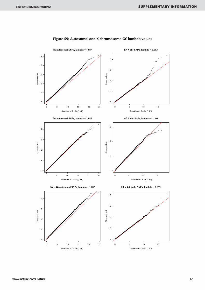
Figure S9: Autosomal and X chromosome GC lambda values
doi: 10.1038/nature08192 SUPPLEMENTARY INFORMATION
www.nature.com/nature 17
7. Imputation analysis of untyped SNPs. We selected 192 regions that had at least one genotyped
SNP with P < 0.0001 in one of the three analyses (EA, AA or combined). Hapmap SNPs in the 192 regions were imputed using MACH 1.0 (http://www.sph.umich.edu/csg/abecasis/mach/index.html). Phased haplotypes for 60 CEU subjects (120 haplotypes) were used as the reference for imputing EA sample genotypes; these haplotypes plus 120 phased YRI haplotypes were used to impute genotypes of AA subjects, who represent admixtures of these two ancestries. Haung et al.23 concluded that for MACH 1.o imputation in 29 world populations, “in most populations, mixtures including individuals from at least two HapMap panels produced the highest imputation accuracy,” consistent with our approach here. Any SNP imputed with information content r2<0.3 was excluded from association analysis because of lack of power. This threshold was recommended in an unpublished earlier paper on MACH 1.0 by the Abecasis group, as providing a good balance between power (retaining well‐imputed data) and accuracy (excluding poorly‐imputed data) . For untyped SNPs or missing genotypes, MACH estimated genotypes conditioning on the flanking markers, as a “dosage” (i.e., the estimate is non‐integer, reflecting the weighted probabilities of each possible genotype). We then used logistic regression to test association between disease status and the estimated genotypic dosage, correcting the population stratification as before (but this was done with a custom program, because non‐integer genotype dosages cannot be submittedto PLINK in an external file). We did not observe larger signals from this analysis except for the SNP rs9394026 that is located in the MHC region.
To perform P‐value meta‐analysis for MGS, ISC and SGENE, we imputed Hapmap SNPs in the six regions (MAD1L1, FXR1, MHC, TCF4, NEK1, PTBP2) and performed logistic regression analysis for EA samples and EA+AA combined samples. For these six regions, we reported the p‐values based on observed genotypic values for genotyped SNPs and the p‐values based on imputed dosage for imputed SNPs.
8. Statistical method for combining p‐values from MGS, ISC and SGENE. For a given SNP, MGS,
ISC and SGENE shared P‐values, direction of allelic effects and the number of cases/controls (Table S14). Because overlapping samples from the three datasets were removed (i.e., the Aberdeen sample was included here only in analyses for ISC and not SGENE), the P‐values from the three studies were independent. We converted the p‐values into Z‐scores taking the allelic direction of the effect into consideration. We then used the following linear combination of Z‐scores to summarize the association signals from three studies:
.1 where 23
22
21332111 =++++= wwwZwZwZwZ
For any given combination of weights ),,( 321 www , )1,0(~ NZ if each Zk follows N(0,1). Let kξ denote
the non‐centrality parameter of Z‐score kZ , i.e. )( kk ZE=ξ for k=1, 2, 3 under an alternative
hypothesis. Then, it is straightforward to show that weights ),,(),,( 321321 ξξξ∝www maximize the
non‐centrality parameter of the combined Z‐score, and hence maximize the power of the combined test. On the other hand, the non‐centrality parameter for a trend test24 is
doi: 10.1038/nature08192 SUPPLEMENTARY INFORMATION
www.nature.com/nature 18

)1(1)]1()[1(2
2/12/11,1,
−+−−
⎥⎦
⎤⎢⎣
⎡= −+
kk
kkk
k
k
k
kkk Rp
ppRnn
nn
nξ .
Here, is the number of cases, is the number of controls, and 1,+kn 1,−kn 1,1, −+ += kkk nnn is the total
number of samples of study k. is the relative risk and is the allele frequency of the controls in
study k. We assumed that the relative risks are consistent across three studies (a fixed effect model) and the allele frequencies were identical across three studies (all from the EA population),
then
kR kp
)( kk ZE=ξ is asymptotically proportional to
2/11,1,2 ⎥⎦
⎤⎢⎣
⎡= −+
k
k
k
kkk n
nnn
nη .
Hence, the asymptotically most powerful test is given by taking the following weights:
2/123
22
21 ][ ηηη
η++
= kkw .
Table S15 gives the sample sizes and optimal weights for MGS, ISC, SGENE for meta‐analysis.
Table S15: Weights and Ns for combining Z‐scores from three GWAS: MGS, ISC, SGENE
# case # control # total weight for EA analysis MGS EA 2681 2653 5334 0.5274668 ISC 3322 3587 6909 0.5999642 SGENE 2005 12837 14842 0.6015162 TOTAL 8008 19077 27085
An exploratory meta‐analysis was also carried out that substituted the MGS EA+AA dataset for the MGS EA dataset. As there are no other large AA GWAS datasets available for meta‐analysis, results will be reported elsewhere.
9. Functional relationships among genes (MGS GWAS). We explored several bioinformatic tools to quantify the functional relationships among genes, and found that they defined different relationships among genes containing SNPs with evidence for association in the MGS GWAS analyses. Improvements in genome annotation will be needed to make such analyses more stable.
We annotated gene relationships of SNPs using SNPPER (http://snpper.chip.org), Genome Variation Scanner (http://gvs.gs.washington.edu/GVS/index.jsp) and the RefSeq gene list http://www.ncbi.nlm.nih.gov/RefSeq/). We explored functional properties of 93 genes with one SNP with P < 0.0001 within 10 kb (European‐ancestry, African American, or combined analyses) using: GeneCards (http://www.genecards.org/), AceView (http://www.ncbi.nlm.nih.gov/IEB/Research/Acembly/) and
doi: 10.1038/nature08192 SUPPLEMENTARY INFORMATION
www.nature.com/nature 19
EntrezGene (http://www.ncbi.nlm.nih.gov/sites/entrez?db=gene).
We supplemented these sources by searching for information on gene relationships using the web‐based tool GRAIL (Gene Relationships Across Implicated Loci; http://www.broad.mit.edu/mpg/grail/; Raychaudhuri, S., et al., under review; http://www.broad.mit.edu/mpg/grail/GRAIL_METHODS.pdf; and 25). GRAIL uses a text search method to search for subsets of genes that are mentioned in PubMed abstracts using similar non‐common words. GRAIL results are available upon request, or can be re‐analyzed by the reader with the current GRAIL version based on any list of genes of interest from this study.
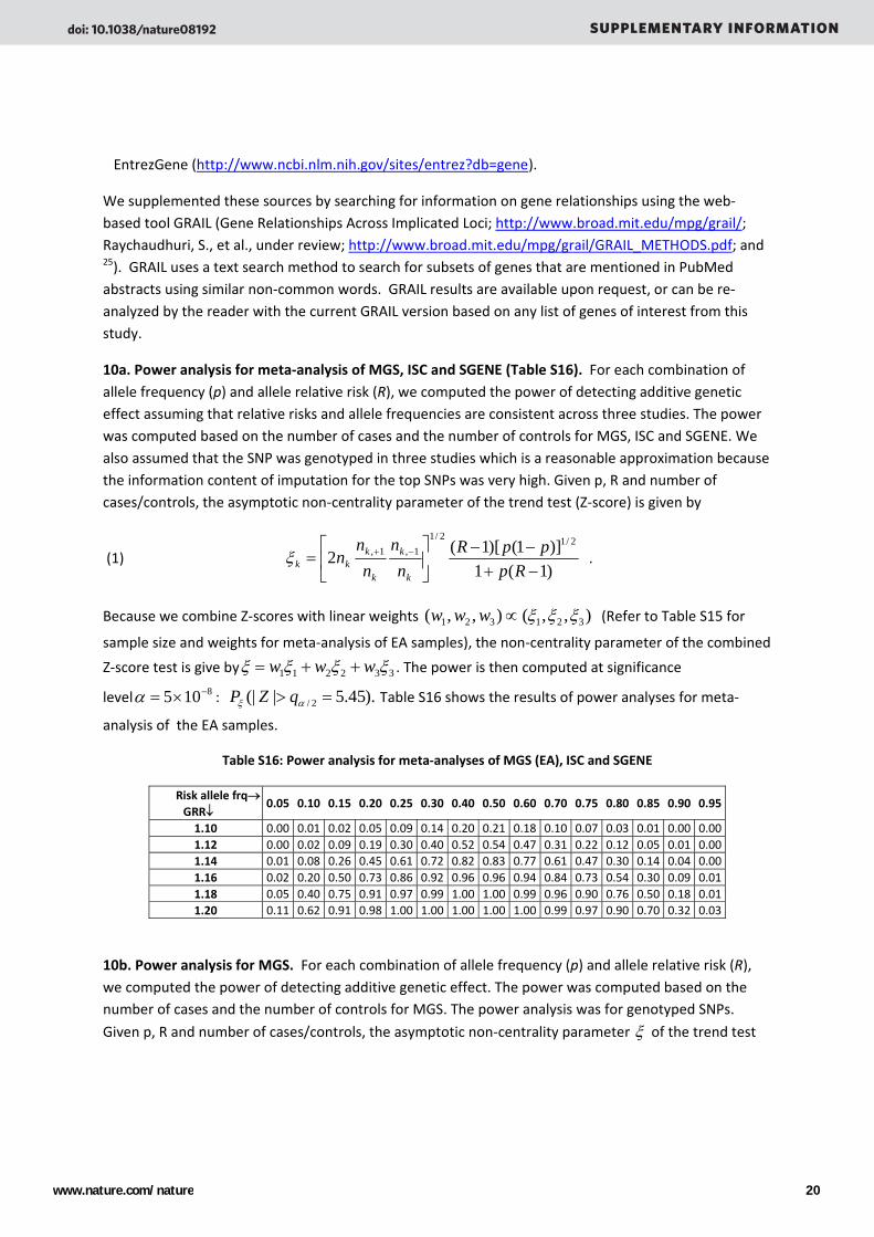
10a. Power analysis for meta‐analysis of MGS, ISC and SGENE (Table S16). For each combination of allele frequency (p) and allele relative risk (R), we computed the power of detecting additive genetic effect assuming that relative risks and allele frequencies are consistent across three studies. The power was computed based on the number of cases and the number of controls for MGS, ISC and SGENE. We also assumed that the SNP was genotyped in three studies which is a reasonable approximation because the information content of imputation for the top SNPs was very high. Given p, R and number of cases/controls, the asymptotic non‐centrality parameter of the trend test (Z‐score) is given by
(1)
)1(1)]1()[1(2
2/12/11,1,
−+−−
⎥⎦
⎤⎢⎣
⎡= −+
RpppR
nn
nn
nk
k
k
kkkξ .
Because we combine Z‐scores with linear weights ),,(),,( 321321 ξξξ∝www (Refer to Table S15 for
sample size and weights for meta‐analysis of EA samples), the non‐centrality parameter of the combined
Z‐score test is give by 332211 ξξξξ www ++= . The power is then computed at significance
level 8105 −×=α : ).45.5|(| 2/ => αξ qZP Table S16 shows the results of power analyses for meta‐
analysis of the EA samples.
Table S16: Power analysis for meta‐analyses of MGS (EA), ISC and SGENE
Risk allele frq→ GRR↓
0.05 0.10 0.15 0.20 0.25 0.30 0.40 0.50 0.60 0.70 0.75 0.80 0.85 0.90 0.95
1.10 0.00 0.01 0.02 0.05 0.09 0.14 0.20 0.21 0.18 0.10 0.07 0.03 0.01 0.00 0.00 1.12 0.00 0.02 0.09 0.19 0.30 0.40 0.52 0.54 0.47 0.31 0.22 0.12 0.05 0.01 0.00 1.14 0.01 0.08 0.26 0.45 0.61 0.72 0.82 0.83 0.77 0.61 0.47 0.30 0.14 0.04 0.00 1.16 0.02 0.20 0.50 0.73 0.86 0.92 0.96 0.96 0.94 0.84 0.73 0.54 0.30 0.09 0.01 1.18 0.05 0.40 0.75 0.91 0.97 0.99 1.00 1.00 0.99 0.96 0.90 0.76 0.50 0.18 0.01 1.20 0.11 0.62 0.91 0.98 1.00 1.00 1.00 1.00 1.00 0.99 0.97 0.90 0.70 0.32 0.03
10b. Power analysis for MGS. For each combination of allele frequency (p) and allele relative risk (R), we computed the power of detecting additive genetic effect. The power was computed based on the number of cases and the number of controls for MGS. The power analysis was for genotyped SNPs.
Given p, R and number of cases/controls, the asymptotic non‐centrality parameter ξ of the trend test
doi: 10.1038/nature08192 SUPPLEMENTARY INFORMATION
www.nature.com/nature 20
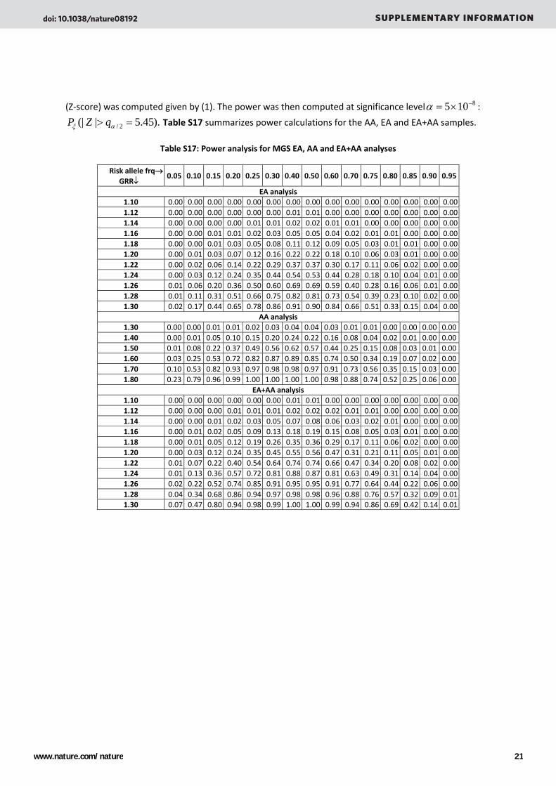
(Z‐score) was computed given by (1). The power was then computed at significance level 8105 −×=α :
).45.5|(| 2/ => αξ qZP Table S17 summarizes power calculations for the AA, EA and EA+AA samples.
Table S17: Power analysis for MGS EA, AA and EA+AA analyses
Risk allele frq→ GRR↓
0.05 0.10 0.15 0.20 0.25 0.30 0.40 0.50 0.60 0.70 0.75 0.80 0.85 0.90 0.95
EA analysis 1.10 0.00 0.00 0.00 0.00 0.00 0.00 0.00 0.00 0.00 0.00 0.00 0.00 0.00 0.00 0.00 1.12 0.00 0.00 0.00 0.00 0.00 0.00 0.01 0.01 0.00 0.00 0.00 0.00 0.00 0.00 0.00 1.14 0.00 0.00 0.00 0.00 0.01 0.01 0.02 0.02 0.01 0.01 0.00 0.00 0.00 0.00 0.00 1.16 0.00 0.00 0.01 0.01 0.02 0.03 0.05 0.05 0.04 0.02 0.01 0.01 0.00 0.00 0.00 1.18 0.00 0.00 0.01 0.03 0.05 0.08 0.11 0.12 0.09 0.05 0.03 0.01 0.01 0.00 0.00 1.20 0.00 0.01 0.03 0.07 0.12 0.16 0.22 0.22 0.18 0.10 0.06 0.03 0.01 0.00 0.00 1.22 0.00 0.02 0.06 0.14 0.22 0.29 0.37 0.37 0.30 0.17 0.11 0.06 0.02 0.00 0.00 1.24 0.00 0.03 0.12 0.24 0.35 0.44 0.54 0.53 0.44 0.28 0.18 0.10 0.04 0.01 0.00 1.26 0.01 0.06 0.20 0.36 0.50 0.60 0.69 0.69 0.59 0.40 0.28 0.16 0.06 0.01 0.00 1.28 0.01 0.11 0.31 0.51 0.66 0.75 0.82 0.81 0.73 0.54 0.39 0.23 0.10 0.02 0.00 1.30 0.02 0.17 0.44 0.65 0.78 0.86 0.91 0.90 0.84 0.66 0.51 0.33 0.15 0.04 0.00
AA analysis 1.30 0.00 0.00 0.01 0.01 0.02 0.03 0.04 0.04 0.03 0.01 0.01 0.00 0.00 0.00 0.00 1.40 0.00 0.01 0.05 0.10 0.15 0.20 0.24 0.22 0.16 0.08 0.04 0.02 0.01 0.00 0.00 1.50 0.01 0.08 0.22 0.37 0.49 0.56 0.62 0.57 0.44 0.25 0.15 0.08 0.03 0.01 0.00 1.60 0.03 0.25 0.53 0.72 0.82 0.87 0.89 0.85 0.74 0.50 0.34 0.19 0.07 0.02 0.00 1.70 0.10 0.53 0.82 0.93 0.97 0.98 0.98 0.97 0.91 0.73 0.56 0.35 0.15 0.03 0.00 1.80 0.23 0.79 0.96 0.99 1.00 1.00 1.00 1.00 0.98 0.88 0.74 0.52 0.25 0.06 0.00
EA+AA analysis 1.10 0.00 0.00 0.00 0.00 0.00 0.00 0.01 0.01 0.00 0.00 0.00 0.00 0.00 0.00 0.00 1.12 0.00 0.00 0.00 0.01 0.01 0.01 0.02 0.02 0.02 0.01 0.01 0.00 0.00 0.00 0.00 1.14 0.00 0.00 0.01 0.02 0.03 0.05 0.07 0.08 0.06 0.03 0.02 0.01 0.00 0.00 0.00 1.16 0.00 0.01 0.02 0.05 0.09 0.13 0.18 0.19 0.15 0.08 0.05 0.03 0.01 0.00 0.00 1.18 0.00 0.01 0.05 0.12 0.19 0.26 0.35 0.36 0.29 0.17 0.11 0.06 0.02 0.00 0.00 1.20 0.00 0.03 0.12 0.24 0.35 0.45 0.55 0.56 0.47 0.31 0.21 0.11 0.05 0.01 0.00 1.22 0.01 0.07 0.22 0.40 0.54 0.64 0.74 0.74 0.66 0.47 0.34 0.20 0.08 0.02 0.00 1.24 0.01 0.13 0.36 0.57 0.72 0.81 0.88 0.87 0.81 0.63 0.49 0.31 0.14 0.04 0.00 1.26 0.02 0.22 0.52 0.74 0.85 0.91 0.95 0.95 0.91 0.77 0.64 0.44 0.22 0.06 0.00 1.28 0.04 0.34 0.68 0.86 0.94 0.97 0.98 0.98 0.96 0.88 0.76 0.57 0.32 0.09 0.01 1.30 0.07 0.47 0.80 0.94 0.98 0.99 1.00 1.00 0.99 0.94 0.86 0.69 0.42 0.14 0.01
doi: 10.1038/nature08192 SUPPLEMENTARY INFORMATION
www.nature.com/nature 21
B. Supplementary Results 1 ‐ MGS GWAS (LD in MHC region; EA+AA analysis)
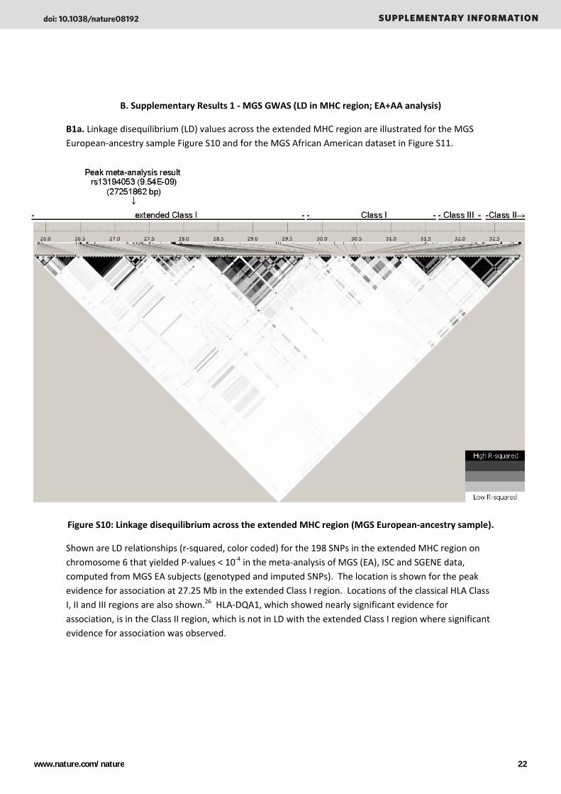
B1a. Linkage disequilibrium (LD) values across the extended MHC region are illustrated for the MGS European‐ancestry sample Figure S10 and for the MGS African American dataset in Figure S11.
Figure S10: Linkage disequilibrium across the extended MHC region (MGS European‐ancestry sample).
Shown are LD relationships (r‐squared, color coded) for the 198 SNPs in the extended MHC region on chromosome 6 that yielded P‐values < 10‐4 in the meta‐analysis of MGS (EA), ISC and SGENE data, computed from MGS EA subjects (genotyped and imputed SNPs). The location is shown for the peak evidence for association at 27.25 Mb in the extended Class I region. Locations of the classical HLA Class I, II and III regions are also shown.26 HLA‐DQA1, which showed nearly significant evidence for association, is in the Class II region, which is not in LD with the extended Class I region where significant evidence for association was observed.
doi: 10.1038/nature08192 SUPPLEMENTARY INFORMATION
www.nature.com/nature 22

Figure S11: MHC region LD and association test results in the MGS African American dataset. Shown are LD data (computed from MGS AA data) for 23 of the 26 SNPs in the LD portion of Figure 1 (3 of the SNPs were not part of the AA dataset), with AA association test results for all genotyped and imputed SNPs in the region. Some evidence for association was observed near TRIM38 and in the FKSG83/POM121L2 region, but support for association is too modest to assume that these results can localize the stronger signal observed in the European‐ancestry meta‐analysis.
doi: 10.1038/nature08192 SUPPLEMENTARY INFORMATION
www.nature.com/nature 23

B1b. MGS combined EA+AA analysis. The genes or nongenic regions containing the best results of the combined EA+AA analysis are shown in Table S18.
Table S18: European-ancestry and African American combined analysis
SNP Chromosome/ Band
Location (BP)
Odds Ratio P-value Gene(s) Function/relevance
rs17833407 9p21.3 21738320 0.814 1.81E-06 (54 kb upstream of MTAP; enzyme involved in polyamine metabolism).
rs1011927 3q26.33 182119438 0.832 1.88E-06 FXR1 Homolog of FMR1 (Fragile X); RNA binding. rs1864744 14q31.3 88020759 0.850 2.18E-06 PTPN21 Regulation of cell growth and differentiation. rs1107592 7p22.3 2007958 0.854 3.84E-06 MAD1L1 Mitotic spindle assembly.
rs7739556 6p22.3 16781577 0.840 3.95E-06 ATXN1 Spinocereballar ataxia type I; interacts with ZNF804A (supported by previous GWAS).27
rs1726206 Xp22.33 3243112 0.813 5.25E-06 MXRA5 Cell adhesion protein.
rs12257761 10q25.3 115006398 0.823 7.25E-06 (90 kb downstream of TCF7L2; Wnt signaling pathway, implicated in type 2 diabetes).
rs2725045 8p23.2 4454742 1.169 8.36E-06 CSMD1 Complement regulation; nerve growth cone; in breakpoint of duplication in autism case.28
rs2587562 8q13.3 73153592 1.157 9.35E-06 TRPA1 Cannabinoid receptor (cannabis may ↑ schizophrenia risk); pain, sound perception.
rs12547975 8p21.2 25686315 0.828 9.59E-06 (71 kb downstream of EBF2; transcription factor in Wnt-responsive LEF1/CTNNB1 pathway).
rs11061935 12p13.33 1684035 0.793 1.06E-05 ADIPOR2 Adiponectin (antidiabetic drug) receptor.
rs7861495 9q13 70344427 1.359 1.17E-05 PGM5 / C9orf71
Component of adherens-type cell-cell and cell-matrix junctions / Transmembrane protein.
Shown are the top results of the MGS analysis that combined European‐ancestry (2681 cases, 2653 controls) and African American (1286 cases, 973 controls) datasets into a combined dataset (3967 cases, 3626 controls) as described above. Shown are the best 12 findings (excluding duplicates ‐‐ SNPs in the same genes or regions but with lesser significance). Shown are genes within 10 kb and comments on function or relevance; or for integenic regions, notes (in parentheses) on genes within 150 kb. The odds ratio is for the tested allele (see Supplementary Datafile 2). Supplementary Datafile 1 contains results for all SNPs with P < 0.001, and full gene names.
We have high confidence in the methods (described above) that were used to estimate ancestry‐related principal components in the combined dataset and to analyze association with these components taken into account. However, complex assumptions must be made in analyses across very different populations (e.g., whether odds ratios are the same or different in the two populations; whether or not the different genotypic “backgrounds” in the populations interact with the tested allele understood). Thus, while this combined analysis can suggest hypotheses about susceptibility loci with effects in both populations, the testing of these hypotheses is probably best accomplished in separate analyses of larger datasets from each population. Unfortunately, there are no comparably large African American SZ datasets at the present time.
The hypotheses suggested by this analysis may be of mechanistic interest. For example, the genic region containing the lowest p‐value contains FXR1 and DNAJC19. FXR1, which encodes an RNA‐binding protein, is a homolog of FMR1. Loss of FMR1 protein (due to large expansions of a CGG repeat in its 5’UTR) causes the Fragile X mental retardation syndrome (FRAXA), which is also the most common known cause of autism.29 The adjacent gene, DNAJC19, is associated with a recessive syndrome of mild mental retardation and cerebellar ataxia.30 However, the result is not genome‐wide significant.
doi: 10.1038/nature08192 SUPPLEMENTARY INFORMATION
www.nature.com/nature 24
Supplementary Results 2: Polygenic score analysis (analysis courtesy of Dr. Shaun Purcell).
Introduction and rationale. The companion paper by the International Schizophrenia Consortium (submitted) reports on a novel form of analysis, which has not been given a formal name but which we refer to here as a polygenic score analysis (PSA). Using this approach, they provide empirical support for the hypothesis that multiple common variants, perhaps a thousand or more, influence risk of schizophrenia, although most of these effects are too small to be detected one SNP at a time. The reader is referred to that paper for full details and results. We provided the authors with access to the full MGS dataset (prior to the expiration of the embargo periods for presentation and publication imposed by dbGAP) for use in their analyses. In one of their key analyses, the ISC sample was the discovery sample for PSA, and MGS‐European ancestry was the target sample. The results demonstrated that across a range of thresholds for selecting the “best” SNPs (ranging from 1% to as many as 50% of the best P‐values in the discovery sample), the set of even slightly “associated” alleles in the ISC sample significantly differentiated cases from controls in the MGS sample (and in other target samples).
Out of interest in this original and thought‐provoking approach, we asked Dr. Shuan Purcell (who developed PSA) to carry out PSA in the reverse direction, with MGS as the discovery sample and ISC as the target sample. Dr. Purcell has provided us with the following summary of results. It is intentionally brief, as it is not independent of the analysis in the ISC paper, and is presented only to further amplify the point that schizophrenia GWAS datasets contain more information about susceptibility alleles than can currently be extracted using single‐SNP analyses of the data. Please see the ISC paper for a full description of the method. (The present authors would also note that Wray et al.31,32 previously studied prediction of disease risk from genome‐wide data, and Janssens and van Duijn33 discussed some limitations of individual prediction. PSA, however, is concerned not with prediction of individual risk, but with evaluating the role of common variants in a disease and the consistency of genetic architecture of common SNP effects across samples. Please see the companion ISC article for details.)
Summary of method. Briefly, quantitative scores are formed that summarize many alleles that are nominally‐associated with increased schizophrenia risk in a “discovery” sample at significance threshold pT (varied from 1‐50%). These scores, the sum of the log of the discovery sample odds ratios, are tested for association with disease state in an independent “target” sample. The discovery analysis (in the MGS‐EA sample here) was a logistic regression of disease on allele dosage, including principal components from EigenStrat as covariates. The ISC target analysis, a logistic regression of disease state on score, controlled for genotyping rate and sample collection site. Using slightly more than 74,000 SNPs that had passed QC in both analyses and that were in approximate linkage equilibrium with each other, we observed a significant association of the pT<0.5 score in the ISC target sample (p = 1.8 X 10‐27, Nagelkerke pseudo R2 = 0.022, see ISC companion manuscript for methodological details and interpretation). Overall, using the same set of SNPs as in the ISC analysis, we observed a trend similar to the one reported by the ISC, in which scores based on increasingly liberal pT thresholds showed stronger association with disease.
doi: 10.1038/nature08192 SUPPLEMENTARY INFORMATION
www.nature.com/nature 25

Supplementary Results 3. Results for specific candidate polymorphisms. In Supplementary Datafile 2, we provide a summary of MGS results for 75 genes that have been mentioned in the literature as candidates for schizophrenia. SNPs in ERBB4 and its ligand neuregulin 1 (NRG1) were both among the top findings in the MGS AA sample (see Table 1 in the main paper).34 Other candidate genes in which at least one SNP produced a P‐value less than 0.0001 include GRM8 and NCAM1 in the European‐ancestry analysis, DTNBP1 (African American) and OPCML (EA+AA combined analysis). Supplementary Datafile 2 also provides details of analyses of a set of candidate polymorphisms that produced at least nominally significant results in a set of meta‐analyses of previous schizophrenia candidate genes by Allen et al. from the SZGENE database.35 They identified 24 such polymorphisms, of which 20 were SNPs, and we had data available for 16 of these in the EA dataset (marked by asterisks in the table), 11 in AA and 9 in the EA+AA dataset. We did not observe support for any of these associations. Finally, we show in the same file our data from the full MGS dataset for the ZNF804A SNP reported by O’Donovan et al.27
Table S19: Candidate polymorphisms based on meta‐analyses of previous studies
Gene Polymorphism Gene Polymorphism APOE APOE (ε2/3/4) E4 vs. E3 GABRB2 rs194072* COMT rs165599 GABRB2 rs6556547* COMT rs737865* GRIN2B rs1019385 (200T/G) DAO rs4623951* GRIN2B rs7301328 (366G/C)* DRD1 rs4532 (DRD1_48A/G)* HP Hp1/2 DRD2 rs1801028 (Ser311Cys) IL1B rs16944 (C511T)* DRD2 rs6277 (Pro319Pro)* MTHFR rs1801131 (A1298C)* DRD4 120‐bp TR MTHFR rs1801133 (C677T)* DRD4 rs1800955 (521T/C) PLXNA2 rs752016* DTNBP1 rs1011313 (P1325)* SLC6A4 5‐HTTVNTR GABRB2 rs1816071* TP53 rs1042522* GABRB2 rs1816072* TPH1 rs1800532 (218A/C)*
doi: 10.1038/nature08192 SUPPLEMENTARY INFORMATION
www.nature.com/nature 26
C. Supplementary References
1 Cloninger, C. R. et al. Genome‐wide search for schizophrenia susceptibility loci: the NIMH Genetics Initiative and Millennium Consortium. Am. J. Med. Genet. 81, 275‐281 (1998).
2 Suarez, B. K. et al. Genomewide linkage scan of 409 European‐ancestry and African American families with schizophrenia: suggestive evidence of linkage at 8p23.3‐p21.2 and 11p13.1‐q14.1 in the combined sample. Am J Hum Genet 78, 315‐333 (2006).
3 Sanders, A. R. et al. No significant association of 14 candidate genes with schizophrenia in a large European ancestry sample: implications for psychiatric genetics. Am J Psychiatry 165, 497‐506 (2008).
4 Maier, W. et al. Continuity and discontinuity of affective disorders and schizophrenia. Results of a controlled family study. Arch. Gen. Psychiatry 50, 871‐883 (1993).
5 Nurnberger, J. I., Jr. et al. Diagnostic interview for genetic studies. Rationale, unique features, and training. NIMH Genetics Initiative. Arch. Gen. Psychiatry 51, 849‐859 (1994).
6 Leckman, J. F., Sholomskas, D., Thompson, W. D., Belanger, A. & Weissman, M. M. Best estimate of lifetime psychiatric diagnosis: a methodological study. Arch. Gen. Psychiatry 39, 879‐883 (1982).
7 Levinson, D. F., Mowry, B. J., Escamilla, M. A. & Faraone, S. V. The Lifetime Dimensions of Psychosis Scale (LDPS): description and interrater reliability. Schizophr. Bull. 28, 683‐695 (2002).
8 Kendler, K. S. et al. The Roscommon Family Study. I. Methods, diagnosis of probands, and risk of schizophrenia in relatives. Arch. Gen. Psychiatry 50, 527‐540 (1993).
9 Levinson, D. F. & Mowry, B. in Genetic Influences on Neural and Behavioral Functions eds D. W. Pfaff, W. Berrettini, T. Joh, & S. Maxson) (CRC Press, 1999).
10 Faraone, S. V. et al. Diagnostic accuracy and confusability analyses: an application to the Diagnostic Interview for Genetic Studies. Psychol. Med. 26, 401‐410 (1996).
11 Kendler, K. S., Karkowski, L. M. & Walsh, D. The structure of psychosis: latent class analysis of probands from the Roscommon Family Study. Arch Gen Psychiatry 55, 492‐499 (1998).
12 Kessler, R. C., Andrews, G., Mroczek, D., Ustun, T.B., Wittchen, H‐U. The World Health Organization Composite International Diagnostic Interview Short Form (CIDI‐SF). International Journal of Methods in Psychiatric Research 7, 171‐185 (1998).
13 Eysenck, S. B. G., Eysenck, H. J. & Barrett, P. A revised version of the psychoticism scale. Pers. Individ. Dif. 6, 21‐29 (1985).
14 McCarroll, S. A. et al. Integrated detection and population‐genetic analysis of SNPs and copy number variation. Nat Genet 40, 1166‐1174 (2008).
15 Korn, J. M. et al. Integrated genotype calling and association analysis of SNPs, common copy number polymorphisms and rare CNVs. Nat Genet 40, 1253‐1260 (2008).
16 Purcell, S. et al. PLINK: a tool set for whole‐genome association and population‐based linkage analyses. Am J Hum Genet 81, 559‐575 (2007).
17 Price, A. L. et al. Principal components analysis corrects for stratification in genome‐wide association studies. Nat. Genet. 38, 904‐909 (2006).
18 Cleveland, W. S., Grosse, E., Shyu, W.M. in Statistical Models in S (ed J.M. Chambers, Hastie, T.J.) Ch. 8, (Chapman & Hall/CRC Press, 1992).
19 Devlin, B. & Roeder, K. Genomic control for association studies. Biometrics 55, 997‐1004 (1999). 20 Dudbridge, F. & Gusnanto, A. Estimation of significance thresholds for genomewide association
scans. Genet Epidemiol 32, 227‐234 (2008). 21 Hoggart, C. J., Clark, T. G., De Iorio, M., Whittaker, J. C. & Balding, D. J. Genome‐wide
significance for dense SNP and resequencing data. Genet Epidemiol 32, 179‐185 (2008).
doi: 10.1038/nature08192 SUPPLEMENTARY INFORMATION
www.nature.com/nature 27

22 Pe'er, I., Yelensky, R., Altshuler, D. & Daly, M. J. Estimation of the multiple testing burden for genomewide association studies of nearly all common variants. Genet Epidemiol 32, 381‐385 (2008).
23 Huang, L. et al. Genotype‐imputation accuracy across worldwide human populations. Am J Hum Genet 84, 235‐250 (2009).
24 Siegmund, D., Yakir, B. The Statistics of Gene Mapping. (Springer, 2007). 25 Raychaudhuri, S. Computational text analysis for functional genomics and bioinformatics.
(Oxford University Press, 2006). 26 Horton, R. et al. Gene map of the extended human MHC. Nat Rev Genet 5, 889‐899 (2004). 27 O'Donovan, M. C. et al. Identification of loci associated with schizophrenia by genome‐wide
association and follow‐up. Nat Genet 40, 1053‐1055 (2008). 28 Glancy, M. et al. Transmitted duplication of 8p23.1‐8p23.2 associated with speech delay, autism
and learning difficulties. Eur J Hum Genet (2008). 29 Bassell, G. J. & Warren, S. T. Fragile X syndrome: loss of local mRNA regulation alters synaptic
development and function. Neuron 60, 201‐214 (2008). 30 Davey, K. M. et al. Mutation of DNAJC19, a human homologue of yeast inner mitochondrial
membrane co‐chaperones, causes DCMA syndrome, a novel autosomal recessive Barth syndrome‐like condition. J Med Genet 43, 385‐393 (2006).
31 Wray, N. R., Goddard, M. E. & Visscher, P. M. Prediction of individual genetic risk to disease from genome‐wide association studies. Genome Res 17, 1520‐1528 (2007).
32 Wray, N. R., Goddard, M. E. & Visscher, P. M. Prediction of individual genetic risk of complex disease. Curr Opin Genet Dev 18, 257‐263 (2008).
33 Janssens, A. C. & van Duijn, C. M. Genome‐based prediction of common diseases: advances and prospects. Hum Mol Genet 17, R166‐173 (2008).
34 Arnold, S. E., Talbot, K. & Hahn, C. G. Neurodevelopment, neuroplasticity, and new genes for schizophrenia. Progress in brain research 147, 319‐345 (2005).
35 Allen, N. C. et al. Systematic meta‐analyses and field synopsis of genetic association studies in schizophrenia: the SzGene database. Nat Genet 40, 827‐834 (2008).
D. Supplementary Acknowledgements ‐ Grant Support We thank the study participants, and the research staff at the study sites. This study was supported by NIH R01 grants (MH67257 to N.G.B., MH59588 to B.J.M., MH59571 to P.V.G., MH59565 to R.F., MH59587 to F.A., MH60870 to W.F.B., MH59566 to D.W.B., MH59586 to J.M.S., MH61675 to D.F.L., MH60879 to C.R.C., and MH81800 to P.V.G.), NIH U01 grants (MH46276 to C.R.C., MH46289 to C. Kaufmann, MH46318 to M.T. Tsuang, MH79469 to P.V.G., and MH79470 to D.F.L.), NARSAD (National Alliance for Research on Schizophrenia and Depression) Young Investigator Awards (to J.D. and A.R.S.), the Genetic Association Information Network (GAIN), and by The Paul Michael Donovan Charitable Foundation. Genotyping was carried out by the Genotyping and Analysis at the Broad Institute of Harvard and MIT (S. Gabriel and D.B.M.), which is supported by grant U54 RR020278 from the National Center for Research Resources. Genotyping of half of the EA sample and almost all the AA sample was carried out with support from GAIN. The GAIN quality control team (G.R. Abecasis and J. Paschall) made important contributions to the project. We thank S. Purcell for assistance with PLINK and for providing details of the Polygenic Score Analysis.
doi: 10.1038/nature08192 SUPPLEMENTARY INFORMATION
www.nature.com/nature 28


![WELCOME [ec.europa.eu]ec.europa.eu/regional_policy/sources/conferences/etc2016/3_project... · 15.15 – 15.20 Welcome – col. Wim Van Zele . 15.20 – 15.40 Presentation MIRG EU](https://img.pdfslide.us/doc/110x75/602196beb088e57d5a22563b/welcome-ec-ec-1515-a-1520-welcome-a-col-wim-van-zele-1520-a-1540.jpg)


![WELCOME [ec.europa.eu]...15.15 – 15.20 Welcome – col. Wim Van Zele . 15.20 – 15.40 Presentation MIRG EU – st. comm. David Brown . 15.40 – 15.50 MIRG EU – Film – maj](https://img.pdfslide.us/doc/110x75/602196beb088e57d5a22563e/welcome-ec-1515-a-1520-welcome-a-col-wim-van-zele-1520-a-1540.jpg)