Halo Orbit Mission Correction Maneuvers

Using Optimal Control

Radu Serban�, Wang S. Koony, Martin W. Loz, Jerrold E. Marsdeny,

Linda R. Petzold�, Shane D. Rossy, and Roby S. Wilsonz

March 31, 2000

Abstract

This paper addresses the computation of the required trajectory correctionmaneuvers (TCM) for a halo orbit space mission to compensate for the launchvelocity errors introduced by inaccuracies of the launch vehicle. By combiningdynamical systems theory with optimal control techniques, we are able to pro-vide a compelling portrait of the complex landscape of the trajectory designspace. This approach enables automation of the analysis to perform paramet-ric studies that simply were not available to mission designers a few years ago,such as how the magnitude of the errors and the timing of the �rst trajectorycorrection maneuver a�ects the correction �V . The impetus for combining dy-namical systems theory and optimal control in this problem arises from designissues for the Genesis Discovery mission being developed for NASA by the JetPropulsion Laboratory.

1 Introduction and Background

1.1 The Genesis Mission

Genesis is a solar wind sample return mission (see Lo et al., [1998]). It is one of

NASA's �rst robotic sample return missions and is scheduled for launch in January

2001 to a halo orbit in the vicinity of the Sun-Earth L1 Lagrange point; L1 is one of

the �ve equilibrium points in the circular restricted three body problem (CRTBP).

See Figure 1 for a depiction of the Genesis trajectory.

In the standard convention, L1 is the unstable equilibrium point between the

Sun and the Earth at roughly 1.5 million km from the Earth in the direction of

�Department of Mechanical and Environmental Engineering, University of California, Santa

Barbara, CA 93106. This research was supported in part by the NSFKDI grant number NSF

ATM-9873133.yControl and Dynamical Systems, Caltech 107-81, Pasadena, CA 91125.zNavigation and Mission Design, Jet Propulsion Laboratory, California Institute of Technology,

M/S 301-140L, 4800 Oak Grove Drive, Pasadena, CA 91109. This research was supported by the

Jet Propulsion Laboratory, California Institute of Technology, under a contract with the National

Aeronautics and Space Administration.

1

L1 L2

x (km)

y(k

m)

-1E+06 0 1E+06

-1E+06

-500000

0

500000

1E+06

L1 L2

x (km)

z(k

m)

-1E+06 0 1E+06

-1E+06

-500000

0

500000

1E+06

y (km)

z(k

m)

-1E+06 0 1E+06

-1E+06

-500000

0

500000

1E+06

0

500000

z (k

m)

-1E+06

0

1E+06

x (km)

-500000

0

500000

y (km)

XY

Z

Figure 1: Genesis Trajectory, XY, XZ, and YZ Projections.

the Sun. Once there, the spacecraft will remain in the halo orbit for two years to

collect solar wind samples before returning them to the Earth for study into the

origins of the solar system. Figure 1 shows three orthographic projections of the

Genesis trajectory: the transfer to the halo, the halo orbit itself, and the return

to Earth. These �gures are plotted in a rotating frame, which is often used in the

study of the three-body problem. The frame is de�ned by �xing the X-axis along

the Sun-Earth line, the Z-axis in the direction normal to the ecliptic, and with the

Y-axis completing a right-handed coordinate system. Viewed from behind the Earth

in the YZ-projection, the orbit appears as a halo around the Sun, hence its name

(originally named for lunar halo orbits by Farquhar).

The Genesis trajectory is the �rst mission to be fully designed using dynamical

systems theory (see Howell, Barden and Lo [1997]). Notice in Figure 1 that the

trajectory travels between neighborhoods of the L1 and L2 libration points with

the purpose of returning the samples to Earth (L2 is roughly 1.5 million km on the

opposite side of the Earth from the Sun). In dynamical systems theory, this is called

a heteroclinic connection between the L1 and L2 regions. One of the attractive

features of this design is the fact that the three year mission, from launch all the way

back to Earth return, requires only a single small deterministic maneuver (less than

6 m/s) when injecting onto the halo orbit! It is extremely di�cult to use traditional

classical algorithms to �nd such a near-optimal solution, so the design of such a

low energy trajectory is facilitated by using dynamical systems methods. This is

achieved by using the stable and unstable manifolds as guides in determining the

end-to-end trajectory.

2

1.2 Halo Orbits

Halo orbits are large three dimensional orbits shaped like the edges of a potato chip.

The Y-amplitude of the Genesis halo orbit, which extends from the X-axis to the

maximum Y-value of the orbit, is about 780,000 km. Note that this is bigger than

the radius of the orbit of the Moon, which is about 380,000 km. The computation

of halo orbits follows standard nonlinear trajectory computation algorithms based

on parallel shooting. Due to the sensitivity of the problem, an accurate �rst guess is

essential, since the halo orbit is actually an unstable orbit (albeit with a fairly long

time constant in the Sun-Earth system). This �rst guess is provided by a high order

analytic expansion of minimum 3rd order using the Lindstedt-Poincar�e method. For

details see Llibre, Martinez and Sim�o [1985], Howell and Pernicka [1988], and Parker

and Chua [1989].

In the CRTBP model, halo orbits are both periodic and time independent. How-

ever, if we take into account all the e�ects of the full solar system, halo orbits are

in fact quasiperiodic and time dependent. Like the L1 equilibrium point, which is

the generator of these families of unstable quasiperiodic orbits, the halo orbit is

also an unstable orbit, behaving dynamically like a saddle point in the directions of

spectrally unstable and stable eigenvalues. There is an entire family of asymptotic

trajectories that departs from the halo orbit called the unstable manifold; there

is also an entire family of asymptotic trajectories which wind onto the halo orbit

called the stable manifold (see, for example, Wiggins [1990]). Each of these families

form a two dimensional surface that is, roughly speaking, a twisted tubular surface

emanating from the halo orbit.

Sim�o, G�omez, Llibre and Martinez [1987] were the �rst to study these invariant

manifolds of the halo orbit and apply them to the design of the SOHO mission.

SOHO did not require the delicate controls provided by this theory, so the actual

mission was own using the classical methods developed at NASA by Farquhar and

Dunham (see, for example, Farquhar, Muhonen, Newman and Heuberger [1980]).

For Genesis, however, these manifolds are absolutely crucial to return the samples

to Earth and land at a speci�ed site (a requirement not imposed on SOHO or

previous libration point missions). The stable manifold, which winds onto the halo

orbit, is used to design the transfer trajectory which delivers the Genesis spacecraft

from launch to insertion onto the halo orbit (HOI). The unstable manifold, which

winds o� of the halo orbit, is used to design the return trajectory which brings

the spacecraft and its precious samples back to Earth via the nearly heteroclinic

connection. See Koon, Lo, Marsden and Ross [2000] for the current state of the

computation of homoclinic and heteroclinic orbits in this problem.

1.3 The Transfer to the Halo Orbit

The transfer trajectory is designed using the following procedure. A halo orbit H(t)

is �rst selected, where t represents time. The stable manifold of H, denoted W s,

consists of a family of asymptotic trajectories which take in�nite time to wind onto

H. These asymptotic solutions cannot be found numerically and are impractical for

space missions where the transfer time needs to be just a few months. However,

3

there is a family of trajectories that lie arbitrarily close toW s that require just a few

months to transfer between Earth and the halo orbit. These trajectories are said

to shadow the stable manifold. It is these shadow trajectories that we can compute

and that are extremely useful to the design of the Genesis transfer trajectory.

A simple way to compute an approximation of W s is provided by Parker and

Chua [1989] and is based on Floquet theory. The basic idea is to linearize the

equations of motion about the periodic orbit and then use the monodromy matrix

provided by Floquet theory to generate a linear approximation of the stable man-

ifold associated with the halo orbit. The linear approximation, in the form of a

state vector, is integrated in the nonlinear equations of motion to produce the ap-

proximation of the stable manifold. In the case of quasiperiodic orbits that are not

too far from periodic orbits, one approximates the orbit as periodic and the same

algorithm is applied to compute approximations of W s (see Howell, Barden and Lo

[1997]; see also G�omez, Masdemont and Sim�o [1993]). For engineering purposes, at

least for space missions, this seems to work well. Recently, a more re�ned approach

based on reduction to the center manifold (or neutrally stable manifold) is provided

by Jorba and Masdemont [1999].

In this paper, we will assume that the halo orbit, H(t), and the stable manifold

M(t) are �xed and provided. Hence we will not dwell further on the theory of their

computation which is well covered in the references (see Howell, Barden, and Lo

[1997]). Instead, let us turn our attention to the trajectory correction maneuver

(TCM) problem.

1.4 The TCM Problem

Genesis will be launched from a Delta 7326 launch vehicle (L/V) using a Thiakol

Star37 motor as the �nal upper stage. The most important error introduced by the

inaccuracies of the launch vehicle is the velocity magnitude error. In this case, the

expected error is 7 m/s (1 sigma value) relative to a boost of approximately 3200

m/s from a 200 km circular altitude Earth orbit. In the space industry, we call the

change in velocity a �V . It is typical in space missions to use the magnitude of the

�V as a measure of the spacecraft performance. The propellant mass is a much

less stable quantity as a measure of spacecraft performance, since it is dependent on

the spacecraft mass and various other parameters which change frequently as the

spacecraft is being built.

Although a 7 m/s error for a 3200 m/s maneuver may seem rather small, it

actually is considered quite large. Unfortunately, one of the characteristics of halo

orbit missions is that, unlike interplanetary mission launches, they are extremely

sensitive to launch errors. Typical interplanetary launches can correct launch vehicle

errors 7 to 14 days after the launch. In contrast, halo orbit missions must generally

correct the launch error within the �rst day after launch, due to energy concerns.

This critical Trajectory Correction Maneuver is called TCM1, being the �rst TCM

of any mission. Two clean up maneuvers, TCM2 and TCM3, generally follow TCM1

after a week or more, depending on the situation.

4

From the equation for a conic orbit,

E =V 2

2�Gm

R; (1)

where E is Keplerian energy, V is velocity, Gm is the gravitational mass, and R is

the position, it can be seen that

�V =�E

V; (2)

where �V and �E denote the variations in velocity and energy, respectively. In

particular, for highly elliptical orbits, V decreases sharply as a function of time past

perigee. Hence, the correction maneuver, �V , grows sharply in inverse proportion

to the time from launch. For a large launch vehicle error, which is possible in the case

of Genesis, the correction maneuver TCM1 can quickly grow beyond the capability

of the spacecraft's propulsion system.

The Genesis spacecraft, built in the spirit of NASA's new low cost mission

approach, is very basic. This makes the performance of an early TCM1 extremely

di�cult and risky. It is highly desirable to delay TCM1 by as long as possible,

even at the expense of expenditure of the precious �V budget. In fact, the Genesis

Project would prefer TCM1 be performed at 2 to 7 days after launch, or later if

at all possible. The design of the current Genesis TCM1 retargets the state after

launch back to the nominal HOI state (see Lo, Williams et al [1998]). This approach

is based on linear analysis and is perfectly adequate if TCM1 is performed within

24 hours after launch. Beyond launch + 24 hours, the correction cost can become

prohibitively high. See also Wilson, Howell, and Lo [1999] for another approach to

targeting that may be applicable for Genesis.

The desire to increase the time between launch and TCM1 suggests that one use

a nonlinear approach, combining dynamical systems theory with optimal control

techniques. We explore two similar but slightly di�erent approaches and are able to

obtain in both cases an optimal maneuver strategy that �ts within the Genesis �V

budget of 150 m/s for the transfer portion of the trajectory. These are:

1. HOI technique: use optimal control techniques to retarget the halo orbit with

the original nominal trajectory as the initial guess.

2. MOI technique: target the stable manifold.

Both methods are shown to yield good results.

2 Optimal Control for Trajectory Correction Maneu-

vers

We now introduce the general problem of optimal control for dynamical systems. We

start by recasting the TCM problem as a spacecraft trajectory planning problem.

Mathematically they are exactly the same. We discuss the spacecraft trajectory

5

planning problem as an optimization problem and highlight the formulation char-

acteristics and particular solution requirements. Then the fuel e�ciency caused by

possible perturbation in the launch velocity and by di�erent delays in TCM1 is

exactly the sensitivity analysis of the optimal solution. COOPT, the software we

use, is an excellent tool in solving this type of problem, both in providing a solu-

tion for the trajectory planning problem with optimal control, and in studying the

sensitivity of di�erent parameters.

We emphasize that the objective in this work is not to design the transfer tra-

jectory, but rather to investigate recovery issues related to possible launch velocity

errors. We therefore assume that a nominal transfer trajectory (corresponding to

zero errors in launch velocity) is available. For the nominal trajectory in our numer-

ical experiments in this paper, we do not use the actual Genesis mission transfer

trajectory, but rather an approximation obtained with a more restricted model. It

has been shown elsewhere (for example, Howell, Barden, and Lo [1997]) that the

general qualitative characteristics found in the restricted models translate well when

extended into more accurate models; we expect the same correlation with this work

as well.

2.1 Recasting TCM as a Trajectory Planning Problem

Althought di�erent from a dynamical systems perspective, the HOI and MOI prob-

lems are very similar once cast as optimization problems. In the HOI problem,

a �nal maneuver (jump in velocity) is allowed at THOI = tmax, while in the MOI

problem, the �nal maneuver takes place on the stable manifold at TMOI < tmax and

no maneuver is allowed at THOI = tmax. A halo orbit insertion trajectory design

problem can be simply posed as:

Find the maneuver times and sizes to minimize fuel consumption

(�V ) for a trajectory starting near Earth and ending on the speci�ed

halo orbit around the Lagrange point L1 of the Sun-Earth system at a

position and with a velocity consistent with the HOI time.

The optimization problem as stated has two important features. First, it involves

discontinuous controls, since the impulsive maneuvers are represented by jumps in

the velocity of the spacecraft. A reformulation of the problem to cast it into the

framework required by continuous optimal control algorithms will be discussed later

in this section. Secondly, the �nal halo orbit insertion time THOI, as well as all

intermediate maneuver times, must be included among the optimization parameters

(p). This too requires further reformulation of the dynamical model to capture the

in uence of these parameters on the solution at a given optimization iteration.

Next, we discuss the reformulations required to solve the HOI discontinuous

control problem; modi�cations of the following procedure required to solve the MOI

problem are discussed in x3.2. We assume that the evolution of the spacecraft is

described by a generic set of six ODEs

x0 = f(t;x); (3)

6

x

y

z H(t)

∆vi+1Ti+1

Ti

T1

∆v1

∆vi

Tn-1

∆vn

Tn

HOI

∆vn-1

Figure 2: Transfer trajectory. Maneuvers take place at times Ti; i = 1; 2; :::; n. In the stable

manifold insertion problem, there is no maneuver at Tn, i.e. �vn = 0.

where x = (xp;xv) 2 R6 contains both positions (xp) and velocities (xv). The

dynamical model of Equation (3) can be either the CRTBP or a more complex

model that incorporates the in uence of the Moon and other planets. In this paper,

we use the CRTBP approximation; other models will be investigated in future work.

To deal with the discontinuous nature of the impulsive control maneuvers, the

equations of motion (e.o.m.) are solved simultaneously on each interval between two

maneuvers. Let the maneuvers M1;M2; :::;Mn take place at times Ti; i = 1; 2; :::; n

and let xi(t); t 2 [Ti�1; Ti] be the solution of Equation (3) on the interval [Ti�1; Ti]

(see Figure 2).

To capture the in uence of the maneuver times on the solution of the e.o.m. and

to be able to solve the e.o.m. simultaneously, we scale the time in each interval by

the duration �Ti = Ti�Ti�1. As a consequence, all time derivatives in Equation (3)

are scaled by 1=�Ti. The dimension of the dynamical system is thus increased to

Nx = 6n.

Position continuity constraints are imposed at each maneuver, that is,

xpi (Ti) = x

pi+1(Ti); i = 1; 2; :::; n � 1: (4)

In addition, the �nal position is forced to lie on the halo orbit (or stable manifold),

that is,

xpn(Tn) = xpH(Tn); (5)

where the halo orbit is parameterized by the HOI time Tn. Additional constraints

dictate that the �rst maneuver (TCM1) is delayed by at least a prescribed amount

TCM1min, that is,

T1 � TCM1min; (6)

and that the order of maneuvers is respected,

Ti�1 < Ti < Ti+1; i = 1; 2; :::; n � 1: (7)

7

With a cost function de�ned as some measure of the velocity discontinuities

�vi = xvi+1(Ti)� xvi (Ti); i = 1; 2; :::; n � 1;

�vn = xvH(Tn)� xvn(Tn);(8)

the optimization problem becomes

minTi;xi;�vi

C(�vi); (9)

subject to the constraints in Equations (4)-(8). More details on selecting the form

of the cost function are given in x3.

2.2 Launch Errors and Sensitivity Analysis

In many optimal control problems, obtaining an optimal solution is not the only

goal. The in uence of problem parameters on the optimal solution (the so called

sensitivity of the optimal solution) is also needed. Sensitivity information provides

a �rst-order approximation to the behavior of the optimal solution when parameters

are not at their optimal values or when constraints are slightly violated.

In the problems treated in this paper, for example, we are interested in estimating

the changes in fuel e�ciency (�V ) caused by possible perturbations in the launch

velocity (�v0) and by di�erent delays in the �rst maneuver (TCM1). As we show in

x3, the cost function is very close to being linear in these parameters (TCM1min and

�v0). Therefore, evaluating the sensitivity of the optimal cost is a very inexpensive

and accurate method of assessing the in uence of di�erent parameters on the optimal

trajectory (especially in our problem).

In coopt, we make use of the Sensitivity Theorem (see Bertsekas [1995]) for

nonlinear programming problems with equality and/or inequality constraints:

Theorem 2.1 Let f , h, and g be twice continuously di�erentiable and consider the

family of problems

minimize f(x)

subject to h(x) = u; g(x) � v;(10)

parameterized by the vectors u 2 Rm and v 2 Rr . Assume that for (u; v) = (0; 0) this

problem has a local minimum x�, which is regular and which together with its asso-

ciated Lagrange multiplier vectors �� and ��, satis�es the second order su�ciency

conditions. Then there exists an open sphere S centered at (u; v) = (0; 0) such that

for every (u; v) 2 S there is an x(u; v) 2 Rn , �(u; v) 2 R

m , and �(u; v) 2 Rr ,

which are a local minimum and associated Lagrange multipliers of problem (10).

Furthermore, x(�), �(�), and �(�) are continuously di�erentiable in S and we have

x(0; 0) = x�; �(0; 0) = ��; �(0; 0) = ��. In addition, for all (u; v) 2 S, there holds

rup(u; v) = ��(u; v);

rvp(u; v) = ��(u; v);(11)

where p(u; v) is the optimal cost parameterized by (u; v),

p(u; v) = f(x(u; v)): (12)

8

The in uence of delaying the maneuver TCM1 is thus directly computed from

the Lagrange multiplier associated with the constraint of Equation (6). To evaluate

sensitivities of the cost function with respect to perturbations in the launch velocity

(�v0), we must include this perturbation explicitly as an optimization parameter and

�x it to some prescribed value through an equality constraint. That is, the launch

velocity is set to

v(0) = vnom0

�1 +

�v0kvnom

0 k

�; (13)

where vnom0 is the nominal launch velocity and

�v0 = �; (14)

for a given �. The Lagrange multiplier associated with the constraint in Equa-

tion (14) yields the desired sensitivity.

2.3 Description of the coopt Software

coopt is a software package for optimal control and optimization of systems mod-

eled by di�erential-algebraic equations (DAE) (see Brenan, Campbell and Petzold

[1995]), developed by the Computational Science and Engineering Group at the Uni-

versity of California, Santa Barbara. It has been designed to control and optimize a

general class of DAE systems, which may be quite large. Here we describe the basic

methods used in coopt. We consider the DAE system

F(t;x;x0;p;u(t)) = 0;

x(t1; r) = x1(r);(15)

where the DAE is index zero, one, or semi-explicit index two (see Ascher and Petzold

[1998], or Brenan, Campbell, and Petzold [1995]) and the initial conditions have been

chosen so that they are consistent (that is, the constraints of the DAE are satis�ed).

The control parameters p and r and the vector-valued control function u(t) must

be determined such that the objective function

Z tmax

t1

(t;x(t);p;u(t)) dt +�(tmax;x(tmax);p; r); (16)

is minimized and some additional inequality constraints

g(t;x(t);p;u(t)) � 0; (17)

are satis�ed. The optimal control function u�(t) is assumed to be continuous. To

represent u(t) in a low-dimensional vector space, we use piecewise polynomials on

[t1; tmax], where their coe�cients are determined by the optimization. For ease of

presentation we can therefore assume that the vector p contains both the parameters

and these coe�cients (we let Np denote the combined number of these values) and

discard the control function u(t) in the remainder of this section. Also, we consider

9

that the initial states are �xed and therefore discard the dependency of x1 on r.

Hence, we consider

F(t;x;x0;p) = 0; x(t1) = x1; (18a)Z tmax

t1

(t;x(t);p) dt +�(tmax;x(tmax);p) is minimized, (18b)

g(t;x(t);p) � 0: (18c)

There are a number of well-known methods for direct discretization of the op-

timal control problem in Equations (18), for the case in which the DAEs can be

reduced to ordinary di�erential equations (ODEs) in standard form. coopt imple-

ments the single shooting method and a modi�ed version of the multiple shooting

method, both of which allow the use of adaptive DAE software.

In the multiple shooting method, the time interval [t1; tmax] is divided into subin-

tervals [ti; ti+1] (i = 1; : : : ; Ntx), and the di�erential equations in Equation (18a)

are solved over each subinterval, where additional intermediate variables Xi are in-

troduced. On each subinterval we denote the solution at time t of Equation (18a)

with initial value Xi at ti by x(t; ti;Xi;p).

Continuity between subintervals in the multiple shooting method is achieved via

the continuity constraints

Ci1(Xi+1;Xi;p) � Xi+1 � x(ti+1; ti;Xi;p) = 0: (19)

The additional constraints of Equation (18c) are required to be satis�ed at the

boundaries of the shooting intervals

Ci2(Xi;p) � g(ti;Xi;p) � 0: (20)

Following common practice, we write

�(t) =

Z t

t1

(�;x(�);p) d�; (21)

which satis�es �0(t) = (t;x(t);p), �(t1) = 0. This introduces another equation

and variable into the di�erential system in Equation (18a). The discretized optimal

control problem becomes

minX2;::: ;XNtx;p

�(tmax) + �(tmax); (22)

subject to the constraints

Ci1(Xi+1;Xi;p) = 0; (23a)

Ci2(Xi;p) � 0: (23b)

This problem can be solved by an optimization algorithm. We use the solver

snopt (see Gill, Murray and Saunders [1997]), which incorporates a sequential

10

µ

1−µ

x

z

y

S

S/C

E

2d

1d

Figure 3: Coordinate frame in the CRTBP approximation.

quadratic programming (SQP) method (see Gill, Murray and Wright [1981]). The

SQP methods require a gradient and Jacobian matrix that are the derivatives of the

objective function and constraints with respect to the optimization variables. We

compute these derivatives via DAE sensitivity software daspk3.0 (Li and Petzold

[1999]). The sensitivity equations to be solved by daspk3.0 are generated via the

automatic di�erentiation software adifor (see Bischof, Carle, Corliss, Griewank

and Hovland [1997]).

This basic multiple-shooting type of strategy can work very well for small-to-

moderate size ODE systems, and has an additional advantage that it is inherently

parallel. However, for large-scale ODE and DAE systems there is a problem because

the computational complexity grows rapidly with the dimension of the ODE system.

coopt implements a highly e�cient modi�ed multiple shooting method (Gill, Jay,

Leonard, Petzold, and Sharma [1998] and Serban [1999]) which reduces the com-

putational complexity to that of single shooting for large-scale problems. However,

we have found it su�cient to use single shooting for the trajectory design problems

treated in this paper.

3 Numerical Results

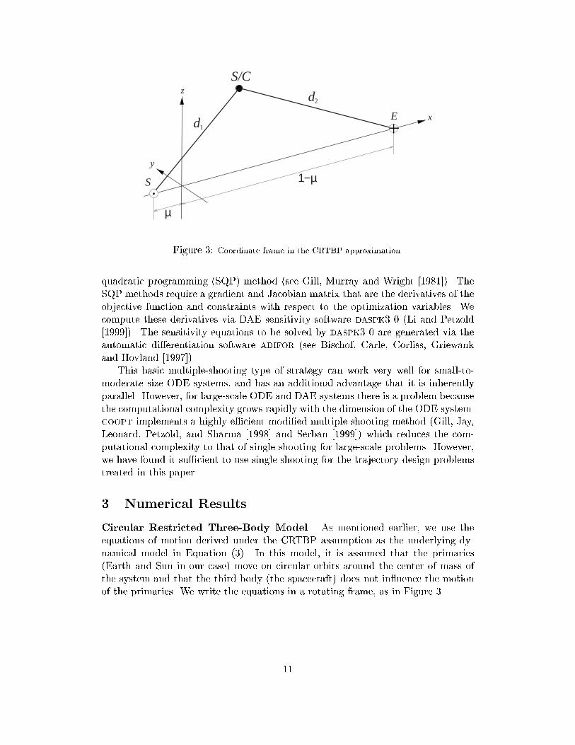
Circular Restricted Three-Body Model. As mentioned earlier, we use the

equations of motion derived under the CRTBP assumption as the underlying dy-

namical model in Equation (3). In this model, it is assumed that the primaries

(Earth and Sun in our case) move on circular orbits around the center of mass of

the system and that the third body (the spacecraft) does not in uence the motion

of the primaries. We write the equations in a rotating frame, as in Figure 3.

11

Using nondimensional units, the equations of motion in the CRTBP model are

_x1 = x4

_x2 = x5

_x3 = x6

_x4 = 2x2 +@U

@x1

_x5 = �2x1 +@U

@x2

_x6 =@U

@x3

(24)

where

x = [x1; x2; x3; x4; x5; x6]T = [x; y; z; vx; vy; vz ]

T

U =1

2(x21 + x22) +

1� �

d1+�

d2

d1 =�(x1 + �)2 + x22 + x23

�1=2d2 =

�(x1 � 1 + �)2 + x22 + x23

�1=2(25)

and � is the ratio between the mass of the Earth and the mass of the Sun-Earth

system,

� =m�

m� +m�

; (26)

where � denotes the Earth and � the Sun. For the Sun-Earth system, we use

� = 3:03591 � 10�6. In the above equations, time is scaled by the period of the

primaries orbits (T=2�, where T = 1 year), positions are scaled by the Sun-Earth

distance (L � d�� = 1:49597927 � 108km), and velocities are scaled by the Earth's

average orbital speed around the Sun (2�L=T = 29:80567km/s).

Choice of Cost Function. At this point we need to give some more details on the

choice of an appropriate cost function for the optimization problem (9). Typically

in space missions, the spacecraft performance is measured in terms of the maneuver

sizes �vi. We consider the following two cost functions.

C1(�v) =

nXi=1

k�vik2 (27)

and

C2(�v) =

nXi=1

k�vik: (28)

While the second of these may seem physically the most meaningful, as it measures

the total sum of the maneuver sizes, such a cost function is nondi�erentiable when-

ever one of the maneuvers vanishes. In our case, this problem occurs already at the

12

�rst optimization iteration, as the initial guess transfer trajectory only has a single

nonzero maneuver at halo insertion. The �rst cost function, on the other hand, is

di�erentiable everywhere.

Although the cost function C1 is more appropriate for the optimizer, it raises

two new problems. Not only is it not as physically meaningful as the cost function

C2, but, in some particular cases, decreasing C1 may actually lead to increases in

C2.

To resolve these issues, we use the following three-stage optimization sequence:

1. Starting with the nominal transfer trajectory as initial guess, and allowing

initially n maneuvers, we minimize C1 to obtain a �rst optimal trajectory, T �1 .

2. Using T �1 as initial guess, we minimize C2 to obtain T �

2 . It is possible that

during this optimization stage some maneuvers can become very small. After

each optimization iteration we monitor the feasibility of the iterate and the

sizes of all maneuvers. As soon as at least one maneuver decreases under

a prescribed threshold (typically 0:1 m/s) at some feasible con�guration, we

stop the optimization algorithm.

3. If necessary, a third optimization stage, using T �2 as initial guess and C2 as

cost function is performed with a reduced number of maneuvers �n (obtained

by removing those maneuvers identi�ed as \zero maneuvers" in step 2).

Merging Optimal Control with Dynamical Systems Theory. Next, we

present results for the halo orbit insertion problem (x3.1) and for the stable mani-

fold insertion problem (x3.2). In both cases we are investigating the e�ect of varying

times for TCM1min on the optimal trajectory, for given perturbations in the nominal

launch velocity. The staggered optimization procedure described above is applied

for values of TCM1min ranging from 1 day to 5 days and perturbations in the mag-

nitude of the launch velocity �v0 ranging from �7 m/s to +7 m/s. We present typical

transfer trajectories, as well as the dependency of the optimal cost on the two pa-

rameters of interest. In addition, using the algorithm presented in x2.2, we perform

a sensitivity analysis of the optimal solution. For the Genesis TCM problem it

turns out that sensitivity information of �rst order is su�cient to characterize the

in uence of TCM1min and �v0 on the spacecraft performance.

The merging of optimal control and dynamical systems has been done through

either (1) the use of the nominal transfer trajectory as a really accurate initial guess,

or (2) the use of the stable invariant manifold.

3.1 Halo Orbit Insertion (HOI) Problem

In this problem we directly target the selected halo orbit with the last maneuver

taking place at the HOI point. Using the optimization procedure described in the

previous section, we compute the optimal cost transfer trajectories for various com-

binations of TCM1min and �v0. In all of our computations, the launch conditions are

those corresponding to the nominal transfer trajectory, i.e.,

13

0.9850.99

0.9951

1.005

-0.01

-0.005

0

0.005

0.01-0.004

-0.002

0

0.002

0.004

xy

z

HOI

TCM1

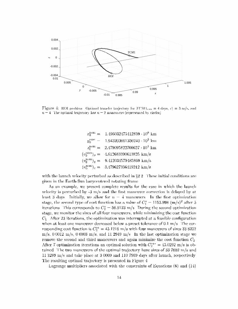
Figure 4: HOI problem. Optimal transfer trajectory for TCM1min = 4 days, �v0 = 3 m/s, and

n = 4. The optimal trajectory has �n = 2 maneuvers (represented by circles).

xnom0 = 1:496032475412839 � 108 km

ynom0 = 1:943203061350240 � 103 km

znom0 = �2:479095822700627 � 103 km

(vnom0 )x = �4:612683390613825 km/s

(vnom0 )y = 9:412034579485869 km/s

(vnom0 )z = �3:479627336419212 km/s

with the launch velocity perturbed as described in x2.2. These initial conditions are

given in the Earth-Sun barycentered rotating frame.

As an example, we present complete results for the case in which the launch

velocity is perturbed by -3 m/s and the �rst maneuver correction is delayed by at

least 3 days. Initially, we allow for n = 4 maneuvers. In the �rst optimization

stage, the second type of cost function has a value of C�1 = 1153:998 (m/s)2 after 5

iterations. This corresponds to C�2 = 50:9123 m/s. During the second optimization

stage, we monitor the sizes of all four maneuvers, while minimizing the cost function

C1. After 23 iterations, the optimization was interrupted at a feasible con�guration

when at least one maneuver decreased below a preset tolerance of 0:1 m/s. The cor-

responding cost function is C��2 = 45:1216 m/s with four maneuvers of sizes 33.8252

m/s, 0.0012 m/s, 0.0003 m/s, and 11.2949 m/s. In the last optimization stage we

remove the second and third maneuvers and again minimize the cost function C2.

After 7 optimization iterations an optimal solution with C���2 = 45:0292 m/s is ob-

tained. The two maneuvers of the optimal trajectory have sizes of 33.7002 m/s and

11.3289 m/s and take place at 3.0000 and 110.7969 days after launch, respectively.

The resulting optimal trajectory is presented in Figure 4.

Lagrange multipliers associated with the constraints of Equations (6) and (14)

14

20

30

40

50

60

70

80

90

100

110

Delay in first maneuver (days)

Pert

urba

tion

in in

itial

vel

ocity

(m

/s)

1 2 3 4 5-7

-6

-5

-4

-3

-2

-1

0

1

2

3

4

5

6

7

12

34

5

-7

0

70

20

40

60

80

100

120

Opt

imal

cos

t C2

(m

/s)

Opt

imal

cos

t C2

(m

/s)

Pert. in initial vel. (m/s)Delay in firs

t maneuver (days)

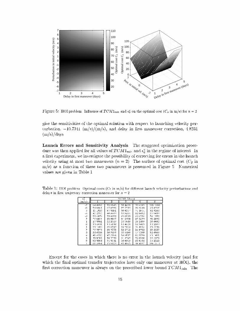
Figure 5: HOI problem. In uence of TCM1min and �v0 on the optimal cost (C2 in m/s) for n = 2.

give the sensitivities of the optimal solution with respect to launching velocity per-

turbation, �10:7341 (m/s)/(m/s), and delay in �rst maneuver correction, 4.8231

(m/s)/days.

Launch Errors and Sensitivity Analysis The staggered optimization proce-

dure was then applied for all values of TCM1min and �v0 in the regime of interest. In

a �rst experiment, we investigate the possibility of correcting for errors in the launch

velocity using at most two maneuvers (n = 2). The surface of optimal cost (C2 in

m/s) as a function of these two parameters is presented in Figure 5. Numerical

values are given in Table 1.

Table 1: HOI problem. Optimal costs (C2 in m/s) for di�erent launch velocity perturbations and

delays in �rst trajectory correction maneuver for n = 2.

�v0

TCM1 (days)(m/s) 1 2 3 4 5

-7 64.8086 76.0845 88.4296 99.6005 109.9305-6 54.0461 67.0226 77.7832 86.8630 95.8202

-5 47.1839 57.9451 66.6277 74.4544 81.8284-4 40.2710 48.8619 55.8274 62.0412 67.9439-3 33.4476 39.8919 45.0290 49.6804 54.1350-2 26.6811 30.9617 34.3489 37.3922 40.3945-1 19.9881 22.2715 23.7848 25.2468 26.66620 13.4831 13.3530 13.4606 13.3465 13.29191 23.1900 21.9242 23.2003 24.4154 25.51362 26.2928 30.2773 33.3203 35.9203 38.33373 34.6338 38.8496 43.5486 47.7200 51.6085

4 41.4230 47.5266 53.9557 62.3780 65.14115 45.9268 56.2245 64.4292 75.0188 81.43256 53.9004 64.9741 76.6978 83.8795 95.23137 61.4084 75.9169 85.4875 98.4197 106.0411

Except for the cases in which there is no error in the launch velocity (and for

which the �nal optimal transfer trajectories have only one maneuver at HOI), the

�rst correction maneuver is always on the prescribed lower bound TCM1min. The

15

95

100

105

110

115

120

125

130

135

1 2 3 4 5

0

1

2

3

4

5

6

7

12

34

5

-7

0

790

100

110

120

130

140

Delay in first maneuver (days)

Pert

urba

tion

in in

itial

vel

ocity

(m

/s)

-7

-6

-5

-4

-3

-2

-1

Hal

o or

bit i

nser

tion

time

(day

s)

Pert. in initial vel. (m/s) Delay in first maneuver (days)

Hal

o or

bit i

nser

tion

time

(day

s)

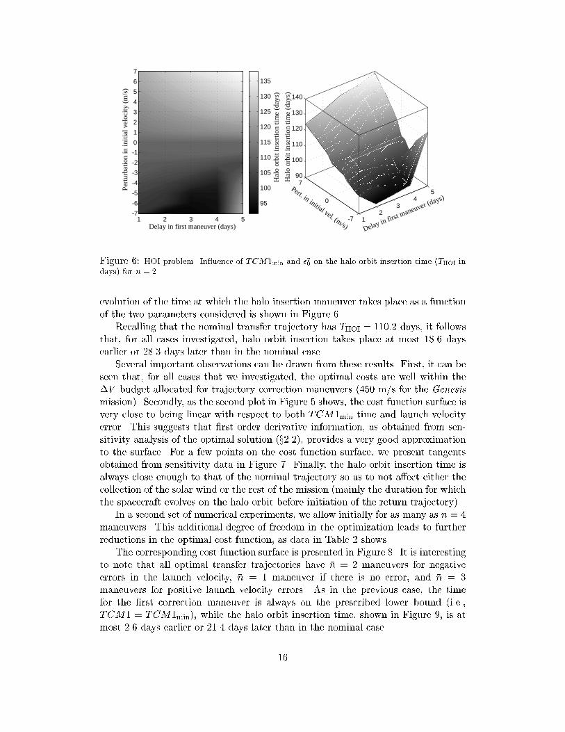
Figure 6: HOI problem. In uence of TCM1min and �v0 on the halo orbit insertion time (THOI in

days) for n = 2.

evolution of the time at which the halo insertion maneuver takes place as a function

of the two parameters considered is shown in Figure 6.

Recalling that the nominal transfer trajectory has THOI = 110:2 days, it follows

that, for all cases investigated, halo orbit insertion takes place at most 18.6 days

earlier or 28.3 days later than in the nominal case.

Several important observations can be drawn from these results. First, it can be

seen that, for all cases that we investigated, the optimal costs are well within the

�V budget allocated for trajectory correction maneuvers (450 m/s for the Genesis

mission). Secondly, as the second plot in Figure 5 shows, the cost function surface is

very close to being linear with respect to both TCM1min time and launch velocity

error. This suggests that �rst order derivative information, as obtained from sen-

sitivity analysis of the optimal solution (x2.2), provides a very good approximation

to the surface. For a few points on the cost function surface, we present tangents

obtained from sensitivity data in Figure 7. Finally, the halo orbit insertion time is

always close enough to that of the nominal trajectory so as to not a�ect either the

collection of the solar wind or the rest of the mission (mainly the duration for which

the spacecraft evolves on the halo orbit before initiation of the return trajectory).

In a second set of numerical experiments, we allow initially for as many as n = 4

maneuvers. This additional degree of freedom in the optimization leads to further

reductions in the optimal cost function, as data in Table 2 shows.

The corresponding cost function surface is presented in Figure 8. It is interesting

to note that all optimal transfer trajectories have �n = 2 maneuvers for negative

errors in the launch velocity, �n = 1 maneuver if there is no error, and �n = 3

maneuvers for positive launch velocity errors. As in the previous case, the time

for the �rst correction maneuver is always on the prescribed lower bound (i.e.,

TCM1 = TCM1min), while the halo orbit insertion time, shown in Figure 9, is at

most 2.6 days earlier or 21.4 days later than in the nominal case.

16

7 6 5 4 3 2 1 0 1 2 3 4 5 6 710

20

30

40

50

60

70

80

90

Perturbation in initial velocity (m/s)1 2 3 4 5

10

20

30

40

50

60

70

80

90

Delay in first maneuver (days)

Opt

imal

cos

t C2

(m

/s)

Opt

imal

cos

t C2

(m

/s)

Figure 7: HOI problem. Sensitivity of the optimal solution for n = 2. Circles correspond to

optimization results. Line segments are predictions based on sensitivity computations. The �gure

on the left was obtained with TCM1min = 3 days and shows the sensitivity of the optimal solution

with respect to �v0 . The �gure on the right was obtained with �v0 = 3 m/s and shows the sensitivity

of the optimal solution with respect to TCM1min.

Table 2: HOI problem. Optimal costs (C2 in m/s) for di�erent launch velocity perturbations and

delays in �rst trajectory correction maneuver for the best case over n = 2; 3; 4.

�v0

TCM1 (days)(m/s) 1 2 3 4 5

-7 61.0946 76.0852 88.4295 99.3123 109.9174

-6 54.0461 67.0212 77.7832 86.8994 95.8202-5 47.1389 57.9277 66.6277 74.4513 81.8572-4 40.2710 48.8619 55.7984 62.0398 67.9438-3 33.3664 39.8919 45.0290 49.6804 54.1357-2 26.6720 30.9617 34.3489 37.3911 40.3945-1 19.9674 22.1091 23.7848 25.2640 26.66180 13.4598 13.2902 13.4428 13.2907 13.29191 19.8257 21.9026 23.2005 24.4149 25.4359

2 26.2933 30.2773 33.3077 35.9203 38.33373 32.8151 38.8496 43.5486 47.7200 51.60854 39.3646 47.5279 53.9557 59.7078 65.11175 45.9127 56.2333 64.4292 71.7790 78.70226 52.4968 64.9741 74.9477 83.8795 92.30907 59.0967 73.7398 85.4875 95.9822 105.8960

17

20

30

40

50

60

70

80

90

100

1 2 3 4 5

0

1

2

3

4

5

6

7

12

34

5

0

70

20

40

60

80

100

Delay in first maneuver (days)

Pert

urba

tion

in in

itial

vel

ocity

(m

/s)

-7

-6

-5

-4

-3

-2

-1

-7

Opt

imal

cos

t C2

(m

/s)

Opt

imal

cos

t C2

(m

/s)

Pert. in initial vel. (m/s)Delay in firs

t maneuver (d

ays)

Figure 8: HOI problem. In uence of TCM1min and �v0 on the optimal cost (C2 in m/s). In each

case, the best trajectory over n = 2; 3; 4 was plotted.

110

115

120

125

130

1 2 3 4 5

0

1

2

3

4

5

6

7

12

34

5

0

7100

110

120

130

140

-7

Delay in first maneuver (days)

Pert

urba

tion

in in

itial

vel

ocity

(m

/s)

-7

-6

-5

-4

-3

-2

-1

Hal

o or

bit i

nser

tion

time

(day

s)

Pert. in initial vel. (m/s)Delay in firs

t maneuver (d

ays)

Hal

o or

bit i

nser

tion

time

(day

s)

Figure 9: HOI problem. In uence of TCM1min and �v0 on the halo orbit insertion time (THOI in

days). In each case, the best trajectory over n = 2; 3; 4 was plotted.

18

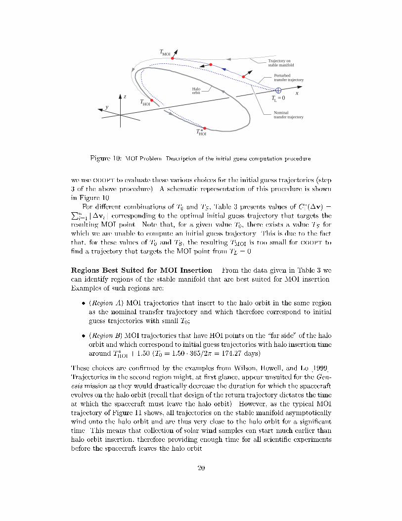
3.2 Stable Manifold Orbit Insertion (MOI) Problem

Obtaining a Good Initial Guess. In the MOI problem the last nonzero ma-

neuver takes place on the stable manifold and there is no maneuver to insert onto

the halo orbit. This implies that, in addition to the constraints of Equation (5)

imposing that the �nal position is on the halo orbit, constraints must be imposed

to match the �nal spacecraft velocity with the velocity on the halo orbit. These

highly nonlinear constraints, together with the fact that a much larger parameter

space is now investigated (we target an entire surface as opposed to just a curve)

make the optimization problem much more di�cult than the one corresponding to

the HOI case. The �rst problem that arises is that the nominal transfer trajectory

is not a good enough initial guess to ensure convergence to an optimum. To obtain

an appropriate initial guess we use the following procedure:

1. We start by selecting an HOI time, THOI. This yields the position and velocity

on the halo orbit.

2. The above position and velocity are perturbed in the direction of the stable

manifold and the equations of motion in Equation (24) are then integrated

backwards in time for a selected duration TS . This yields an MOI point which

is now �xed in time, position, and velocity.

3. For a given value of TCM1min and with �v0 = 0, and using the nominal transfer

trajectory as initial guess, we use coopt to �nd a trajectory that targets this

MOI point, while minimizing C1.

With the resulting trajectory as an initial guess and the desired value of �v0 we

proceed with the staggered optimization presented before to obtain the �nal optimal

trajectory for insertion on the stable manifold. During the three stages of the

optimization procedure, both the MOI point and the HOI point are free to move (in

position, velocity, and time) on the stable manifold surface and on the halo orbit,

respectively.

The fact that we are using local optimization techniques implies that the com-

puted optimal trajectories are very sensitive to the choice of the initial guess tra-

jectory. For given values of the problem parameters (such as initial number of

maneuvers, perturbation in launch velocity, and lower bound on TCM1) we �nd op-

timal trajectories in a neighborhood of the initial guess trajectory. In other words,

computed optimal trajectories can be `steered' towards regions of interest by appro-

priate choices of initial guess trajectories. For example, taking the launch time to

be TL = 0 and the HOI time (T �HOI

) of the nominal transfer trajectory as a refer-

ence point on the halo orbit, we can investigate a given zone of the design space by

an appropriate choice of the HOI point of our initial guess trajectory with respect

to T �HOI

(step 1 of the above procedure). That is, we select a value T0 such that

THOI = T �HOI

+ T0. The point where the initial guess trajectory inserts onto the

stable manifold is then de�ned by selecting the duration TS for which the equations

of motion are integrated backwards in time (step 2 of the above procedure). This

gives a stable manifold insertion time of TMOI = THOI�TS = T �HOI

+T0�TS . Next,

19

x

y

z

TMOI

THOI

THOI*

Trajectory on stable manifold

Nominal transfer trajectory

Haloorbit

T = 0L

Perturbedtransfer trajectory

Figure 10: MOI Problem. Description of the initial guess computation procedure.

we use coopt to evaluate these various choices for the initial guess trajectories (step

3 of the above procedure). A schematic representation of this procedure is shown

in Figure 10.

For di�erent combinations of T0 and TS , Table 3 presents values of C�1 (�v) =Pn

i=1 k�vik corresponding to the optimal initial guess trajectory that targets the

resulting MOI point. Note that, for a given value T0, there exists a value TS for

which we are unable to compute an initial guess trajectory. This is due to the fact

that, for these values of T0 and TS , the resulting TMOI is too small for coopt to

�nd a trajectory that targets the MOI point from TL = 0.

Regions Best Suited for MOI Insertion. From the data given in Table 3 we

can identify regions of the stable manifold that are best suited for MOI insertion.

Examples of such regions are:

� (Region A) MOI trajectories that insert to the halo orbit in the same region

as the nominal transfer trajectory and which therefore correspond to initial

guess trajectories with small T0;

� (Region B) MOI trajectories that have HOI points on the \far side" of the halo

orbit and which correspond to initial guess trajectories with halo insertion time

around T �HOI

+ 1:50 (T0 = 1:50 � 365=2� = 174:27 days).

These choices are con�rmed by the examples from Wilson, Howell, and Lo [1999].

Trajectories in the second region might, at �rst glance, appear unsuited for the Gen-

esis mission as they would drastically decrease the duration for which the spacecraft

evolves on the halo orbit (recall that design of the return trajectory dictates the time

at which the spacecraft must leave the halo orbit). However, as the typical MOI

trajectory of Figure 11 shows, all trajectories on the stable manifold asymptotically

wind onto the halo orbit and are thus very close to the halo orbit for a signi�cant

time. This means that collection of solar wind samples can start much earlier than

halo orbit insertion, therefore providing enough time for all scienti�c experiments

before the spacecraft leaves the halo orbit.

20

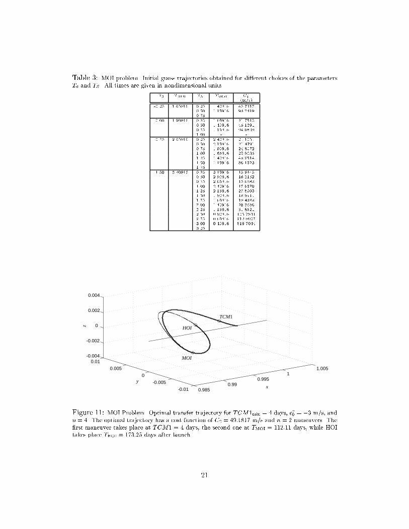
Table 3: MOI problem. Initial guess trajectories obtained for di�erent choices of the parameters

T0 and TS . All times are given in nondimensional units.

T0 THOI TS TMOI C�1

(m/s)

-0.25 1.65916 0.25 1.40916 45.73170.50 1.15916 93.24190.75 - -

0.00 1.90916 0.25 1.65916 21.75150.50 1.40916 45.1291

0.75 1.15916 94.08391.00 - -

0.75 2.65916 0.25 2.40916 21.10510.50 2.15916 21.47910.75 1.90916 24.80721.00 1.65916 23.9035

1.25 1.40916 43.25141.50 1.15916 86.13231.75 - -

1.50 3.40916 0.25 3.15916 15.91450.50 2.90916 16.21520.75 2.65916 15.6983

1.00 2.40916 17.63701.25 2.15916 27.59031.50 1.90916 18.97111.75 1.65916 19.42832.00 1.40916 28.36862.25 1.15916 51.85212.50 0.90916 105.78312.75 0.65916 212.9997

3.00 0.40916 519.70443.25 - -

0.9850.99

0.9951

1.005

-0.01

-0.005

0

0.005

0.01-0.004

-0.002

0

0.002

0.004

xy

z

MOI

HOI

TCM1

Figure 11: MOI Problem. Optimal transfer trajectory for TCM1min = 4 days, �v0 = �3 m/s, and

n = 4. The optimal trajectory has a cost function of C2 = 49:1817 m/s and �n = 2 maneuvers. The

�rst maneuver takes place at TCM1 = 4 days, the second one at TMOI = 112:11 days, while HOI

takes place THOI = 173:25 days after launch.

21

Table 4: MOI problem. Optimal costs (C2 in m/s) for di�erent launching velocity perturbations

and delays in �rst trajectory correction maneuver.

TCM1min(days) �v0(m/s) C2 (m/s)

3 -3 45.1427-4 55.6387

-5 65.9416-6 76.7144-7 87.3777

4 -3 49.1817-4 61.5221-5 73.4862

-6 85.7667-7 99.3405

5 -3 53.9072-4 66.8668-5 81.1679-6 94.3630

-7 109.2151

Once we select a region of the stable manifold by selecting an appropriate initial

guess trajectory, we can perform the same type of analysis as done for the HOI

problem of x3.1. In what follows, we consider the case in which we correct for

perturbations in launch velocity by seeking optimal MOI trajectories in Region B,

that is, on the far side of the halo from the Earth. For given values of �v0 and

TCM1min, we �rst compute an MOI initial guess trajectory with T0 = 1:50 and

TS = 0:75 and then use the staggered optimization procedure described in x3 to �nd

an optimal MOI trajectory in this vicinity.

We present results from such computations in Table 4. It can be seen that the

optimal MOI trajectories are very close (in terms of their associated cost function

C2) to the corresponding HOI trajectories. These results can be understood if we

recall that the nominal transfer trajectory that we use in our experiments actually

inserts onto the halo orbit directly as opposed to the manifold. To take full advantage

of the stable manifold in correcting for launching errors, one may need to start with

a nominal transfer trajectories that insert onto the stable manifold. For missions

that are designed to have such nominal transfer trajectories, correction trajectories

that also insert onto the stable manifold are expected to be much more e�cient than

those obtained with the current formulation of the problem.

4 Conclusions and Future Work

This paper explores new approaches for automated parametric studies of optimal

trajectory correction maneuvers for a halo orbit mission. Using the halo orbit in-

sertion approach, for all the launch velocity errors and TCM1min considered we

found optimal recovery trajectories. The cost functions (fuel consumption in terms

of �V ) are within the allocated budget even in the worst case (largest TCM1minand largest launch velocity error).

Using the stable manifold insertion approach, we obtained similar results to

those found using HOI targeted trajectories. The failure of the MOI approach to

reduce the �V signi�cantly may be because the optimization procedure (even in

the HOI targeted case) naturally �nds trajectories `near' the stable manifold. We

will investigate this interesting e�ect in future work.

22

The main contribution of dynamical systems theory to the problem of �nding

optimal recovery trajectories is in the construction of good initial guess trajectories

in sensitive regions which allows the optimizer to hone in on the solution. We feel

that this aspect of our work will be important in many other future mission design

problems. Many missions in the future will also require the use of optimal control in

the context of low thrust. The software and methods of this paper can be used with

little change for such problems. In fact, the techniques of this paper are applicable

to a variety of problems. We plan to investigate these and related issues in future

publications.

Acknowledgments. This work was carried out at the Computational Science and

Engineering Group at the University of California, Santa Barbara, the Jet Propul-

sion Laboratory and the California Institute of Technology. The work was partially

supported by the Caltech President's fund, the NASA Advanced Concepts Research

Program, The Genesis Project, NSF grant KDI/ATM-9873133 and AFOSR Mi-

crosat contract F49620-99-1-0190.

References

Ascher, U. M. and L. R. Petzold [1998] Computer Methods for Ordinary Di�erential

Equations and Di�erential-Algebraic Equations, SIAM, 1998.

Ascher, U. M., R.M.M. Mattheij, and R. D. Russell, Numerical Solution of Bound-

ary Value Problems for Ordinary Di�erential Equations, Society for Industrial

and AppliedMathematics (SIAM) Publications, Philadelphia, PA, 1995. ISBN

0-89871-354-4.

Bertsekas, D.R. [1995] Nonlinear Programming, Athena Scienti�c, Belmont, Ma.

Bischof, C., A. Carle, G. Corliss, A. Griewank, and P. Hovland [1992], ADIFOR|

generating derivative codes from Fortran programs, Scienti�c Programming, 1,

11{29.

Bischof, C., A. Carle, P. Hovland, P. Khademi, and A. Mauer [1998] ADIFOR

2.0 Users' Guide, MCS Division, Argonne National Laboratory, Technical

Memorandum No. 192, June 1998.

Brenan, K. E., S. L. Campbell, and L. R. Petzold [1995] Numerical Solution

of Initial-Value Problems in Di�erential-Algebraic Equations, SIAM Publi-

cations, Philadelphia, second ed.

Farquhar, R.W., D.P. Muhonen, C.R. Newman and H.S. Heuberger [1980] Trajec-

tories and orbital maneuvers for the �rst libration-point satellite, J. Guidance

and Control. 3, 549{554

Gill, P. E., L. O. Jay, M. W. Leonard, L. R. Petzold and V. Sharma [1998] An

SQP Method for the Optimal Control of Large-Scale Dynamical Systems, J.

Comp. Appl. Math., to appear.

23

Gill, P. E., W. Murray, and M. A. Saunders [1997] SNOPT: An SQP algorithm for

large-scale constrained optimization, Numerical Analysis Report 97-2, Depart-

ment of Mathematics, University of California, San Diego, La Jolla, CA.

Gill, P. E., W. Murray, and M. A. Saunders [1998], User's Guide for SNOPT 5.3:

A Fortran Package for Large-Scale Nonlinear Programming, Department of

Mathematics, University of California, San Diego, La Jolla, CA.

Gill, P. E., W. Murray, and M. H. Wright [1981], Practical Optimization, Academic

Press, London and New York.

G�omez, G., J. Masdemont and C. Sim�o [1993], Study of the transfer from the Earth

to a halo orbit around the equilibrium point L1, Cel. Mech. and Dyn. Astro.

56, 541{562 and 95, (1997), 117{134.

Howell, K. C., B. Barden and M. Lo [1997] Application of dynamical systems

theory to trajectory design for a libration point mission, The Journal of the

Astronautical Sciences 45(2), 161{178.

Howell, K. C. and H. J. Pernicka [1988] Numerical Determination of Lissajous

Trajectories in the Restricted Three-Body Problem, Celestial Mechanics, 41,

107{124.

Jorba, �A. and J. Masdemont [1999] Dynamics in the center manifold of the collinear

points of the restricted three body problem, Physica D , 132, 189{213.

Koon, W.S., M.W. Lo, J.E. Marsden and S.D. Ross [2000] Heteroclinic connec-

tions between periodic orbits and resonance transitions in celestial mechanics,

Chaos, to appear.

Li, S. and L.R. Petzold [1999] Design of New DASPK for Sensitivity Analysis, J.

Comp. Appl. Math., submitted.

Llibre, J., R. Martinez and C. Sim�o [1985] Transversality of the invariant manifolds

associated to the Lyapunov family of periodic orbits near L2 in the restricted

three-body problem, Journal of Di�erential Equations 58, 104-156.

Lo, M., B.G. Williams, W.E. Bollman, D. Han, Y. Hahn, J.L. Bell, E.A. Hirst, R.A.

Corwin, P.E. Hong, K.C. Howell, B. Barden, and R. Wilson [1998] Genesis

Mission Design, Paper No. AIAA 98-4468.

Maly, T. and L. R. Petzold [1996] Numerical methods and software for sensitivity

analysis of di�erential-algebraic systems, Applied Numerical Mathematics 20,

57{79.

Parker, T. S. and L. O. Chua [1989] Practical Numerical Algorithms for Chaotic

Systems, Springer-Verlag, New York.

24

Petzold, L.R., J. B. Rosen, P. E. Gill, L. O. Jay and K. Park [1997] Numerical

Optimal Control of Parabolic PDEs using DASOPT, Large Scale Optimization

with Applications, Part II: Optimal Design and Control, Eds. L. Biegler, T.

Coleman, A. Conn and F. Santosa, IMA Volumes in Mathematics and its

Applications, 93, 271{300.

Serban, R. [1999] COOPT - Control and Optimization of Dynamic Systems - Users'

Guide, Report UCSB-ME-99-1, UCSB Department of Mechanical and Envi-

ronmental Engineering.

Sim�o, C., G. G�omez, J. Llibre and R. Martinez [1987] Station keeping of a quasiperi-

odic halo orbit using invariant manifolds. N87-25362.

Wiggins, S. [1990] Introduction to Applied Nonlinear Dynamical Systems and Chaos.

Texts Appl. Math. Sci. 2, Springer-Verlag.

Wilson, R.S., K.C. Howell, M.W. Lo [1999] Optimization of Insertion Cost for

Transfer Trajectories to Libration Point Orbits Paper No. AAS 99-401.

25