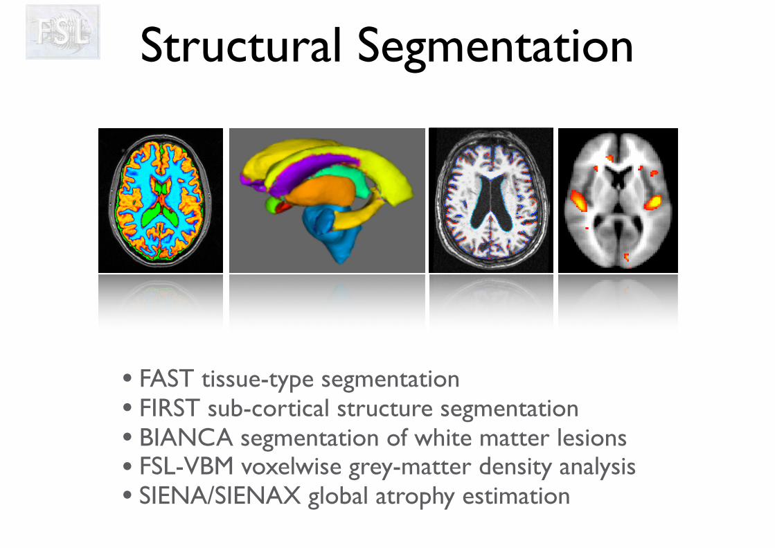
Structural Segmentation

• FAST tissue-type segmentation• FIRST sub-cortical structure segmentation• BIANCA segmentation of white matter lesions• FSL-VBM voxelwise grey-matter density analysis• SIENA/SIENAX global atrophy estimation

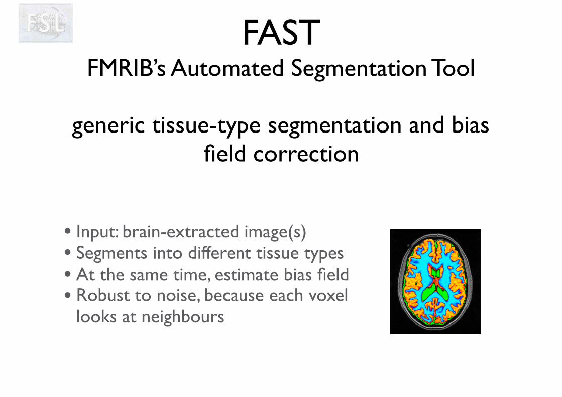
FAST FMRIB’s Automated Segmentation Tool

generic tissue-type segmentation and bias field correction

• Input: brain-extracted image(s)• Segments into different tissue types• At the same time, estimate bias field• Robust to noise, because each voxel

looks at neighbours

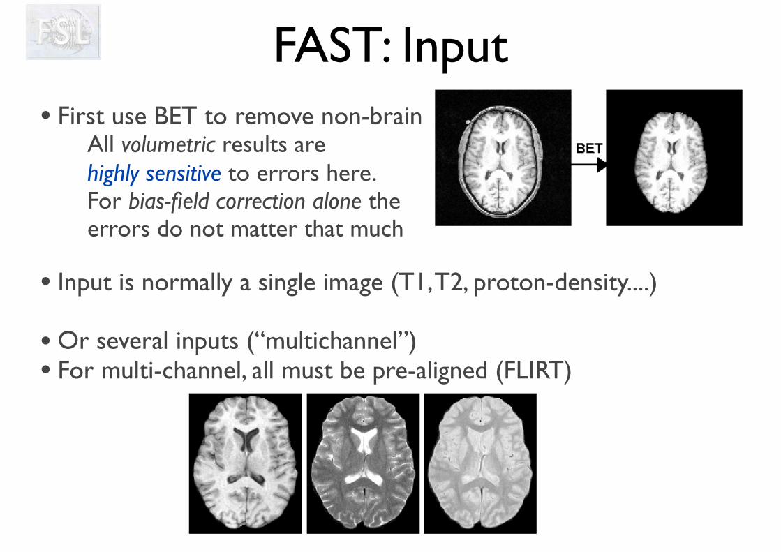
FAST: Input• First use BET to remove non-brain

All volumetric results are highly sensitive to errors here.For bias-field correction alone the errors do not matter that much

• Input is normally a single image (T1, T2, proton-density....)

• Or several inputs (“multichannel”)• For multi-channel, all must be pre-aligned (FLIRT)

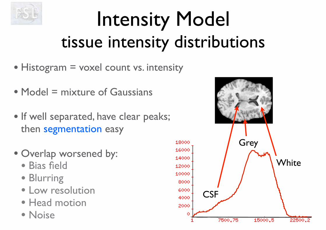
Intensity Model tissue intensity distributions

• Histogram = voxel count vs. intensity

• Model = mixture of Gaussians

• If well separated, have clear peaks; then segmentation easy

• Overlap worsened by:• Bias field• Blurring• Low resolution• Head motion• Noise

CSF

Grey

White

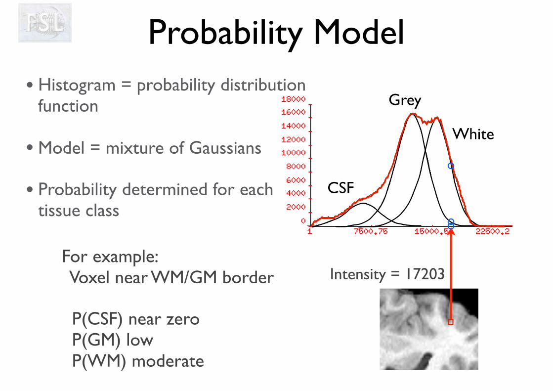
Probability Model• Histogram = probability distribution

function

• Model = mixture of Gaussians

• Probability determined for each tissue class

CSF

Grey

White

For example: Voxel near WM/GM border

P(CSF) near zero P(GM) low P(WM) moderate

Intensity = 17203

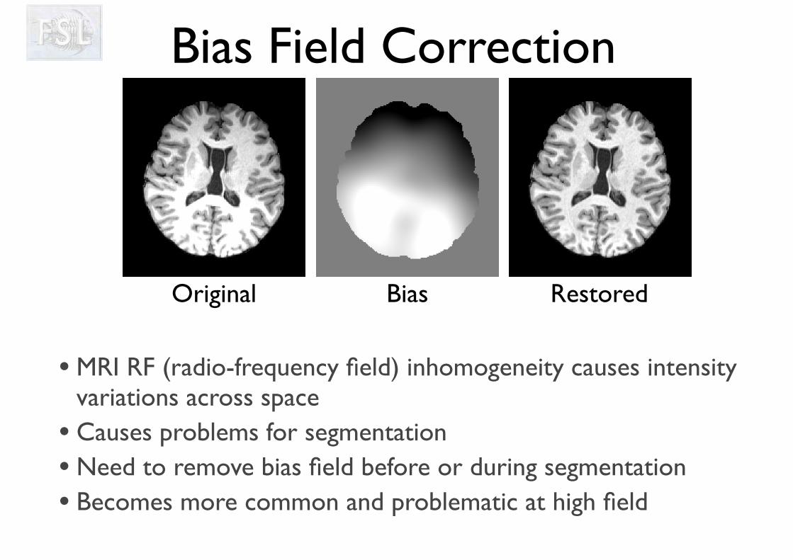
Bias Field Correction

Original Bias Restored

• MRI RF (radio-frequency field) inhomogeneity causes intensity variations across space

• Causes problems for segmentation• Need to remove bias field before or during segmentation• Becomes more common and problematic at high field

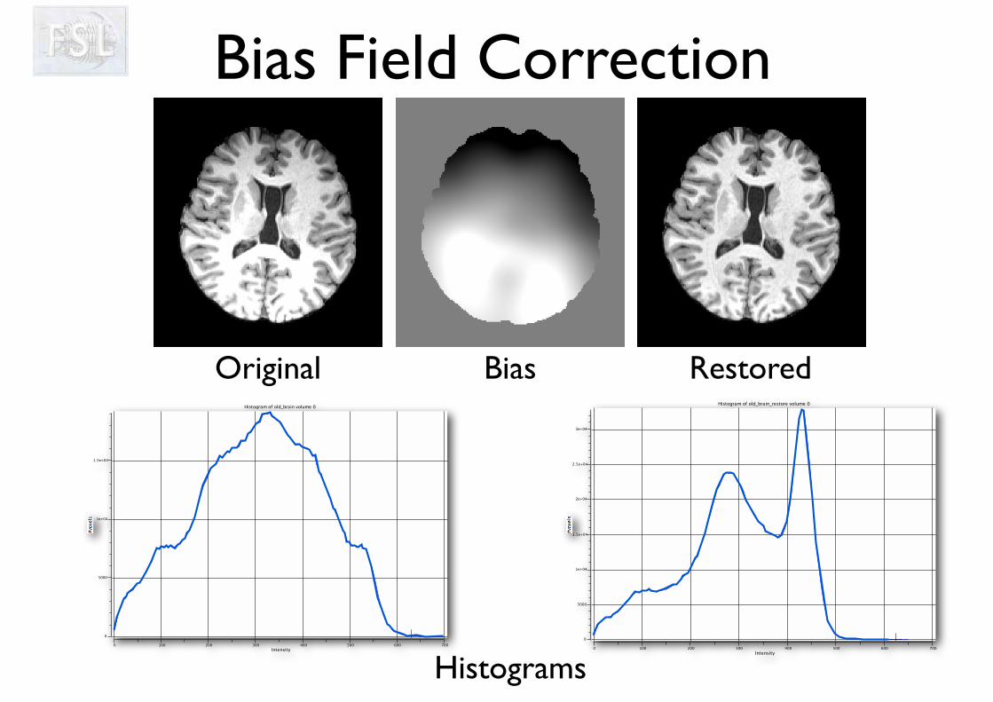
Bias Field Correction

Original Bias RestoredHistogram of old_brain volume 0

0

5000

1e+04

1.5e+04

Intensity0 100 200 300 400 500 600 700

Histogram of old_brain_restore volume 0

0

5000

1e+04

1.5e+04

2e+04

2.5e+04

3e+04

Intensity0 100 200 300 400 500 600 700

Histograms

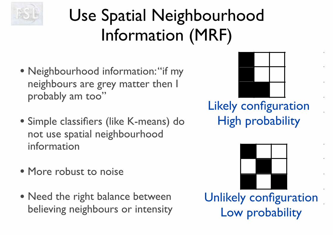
Use Spatial Neighbourhood Information (MRF)

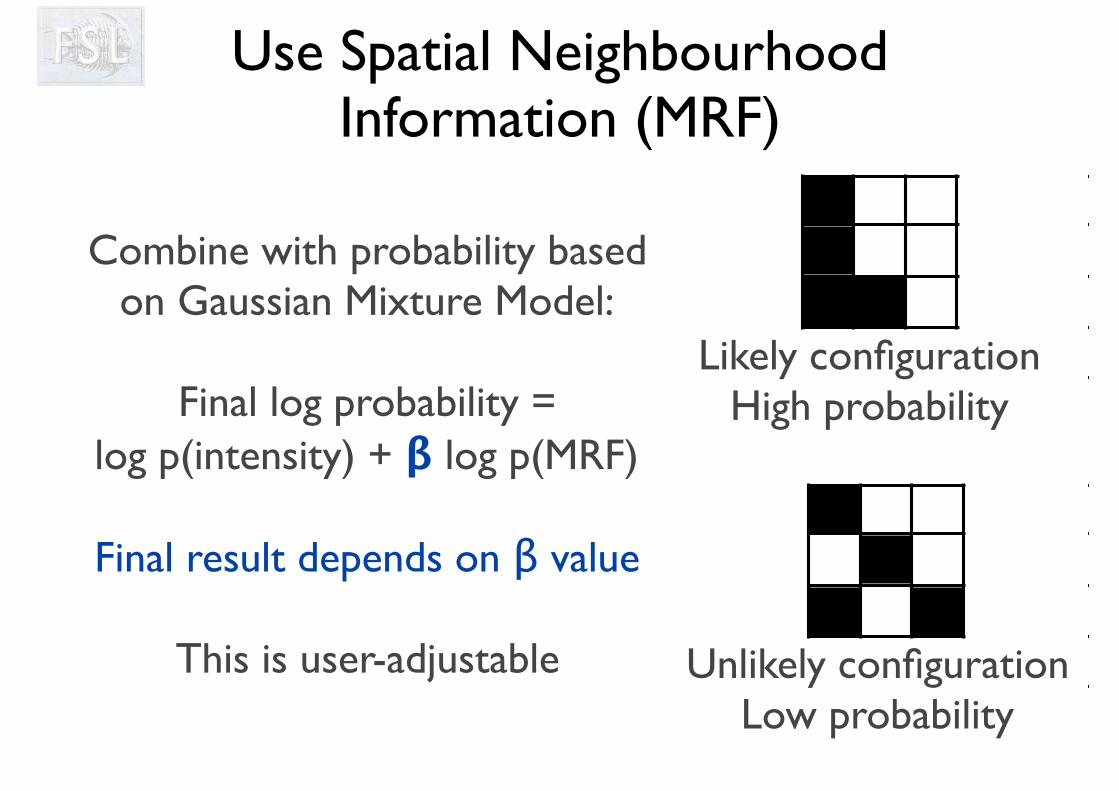
• Neighbourhood information: “if my neighbours are grey matter then I probably am too”

• Simple classifiers (like K-means) do not use spatial neighbourhood information

• More robust to noise

• Need the right balance between believing neighbours or intensity

Likely configurationHigh probability

Unlikely configurationLow probability

Use Spatial Neighbourhood Information (MRF)

Likely configurationHigh probability

Unlikely configurationLow probability

Combine with probability based on Gaussian Mixture Model:

Final log probability =log p(intensity) + β log p(MRF)

Final result depends on β value

This is user-adjustable

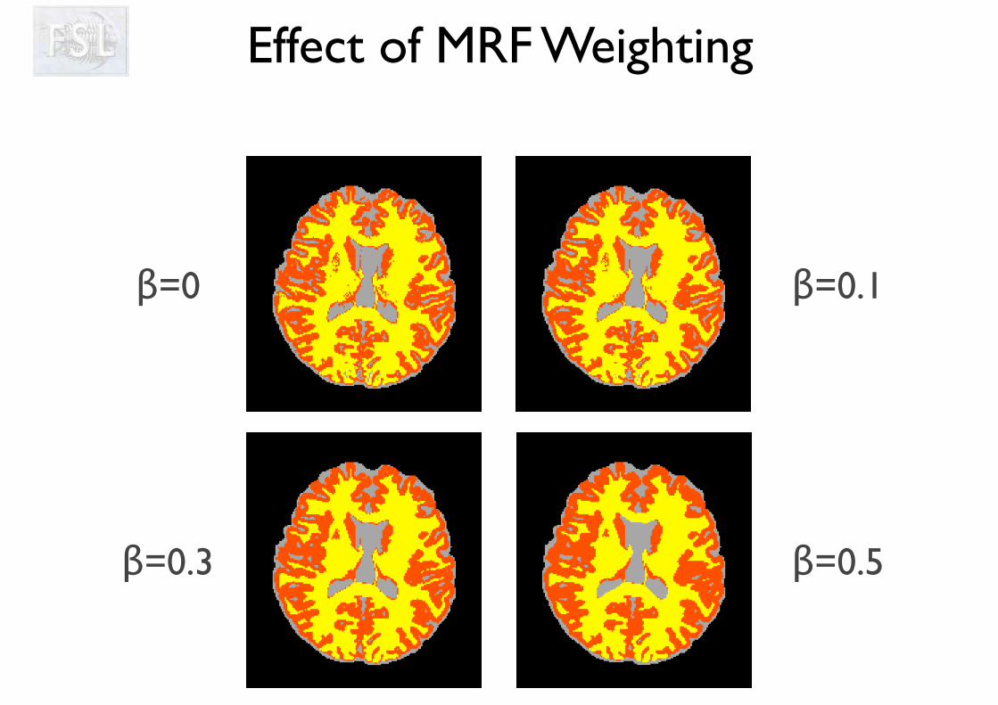
Effect of MRF Weighting

β=0

β=0.3

β=0.1

β=0.5

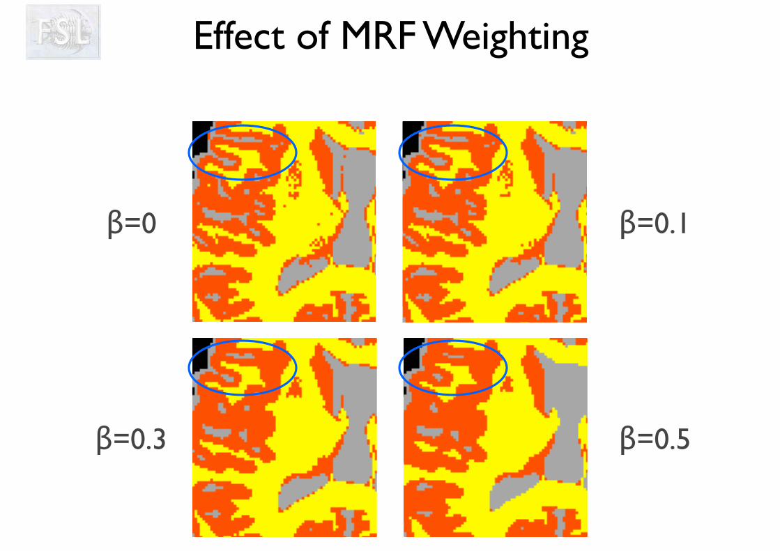
Effect of MRF Weighting

β=0

β=0.3

β=0.1

β=0.5

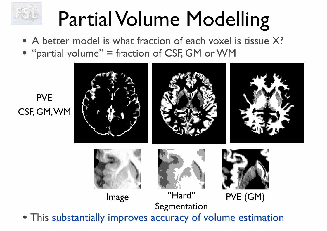
Partial Volume Modelling• A better model is what fraction of each voxel is tissue X?• “partial volume” = fraction of CSF, GM or WM

• This substantially improves accuracy of volume estimation

Image “Hard” Segmentation

PVE (GM)

PVE

CSF, GM, WM

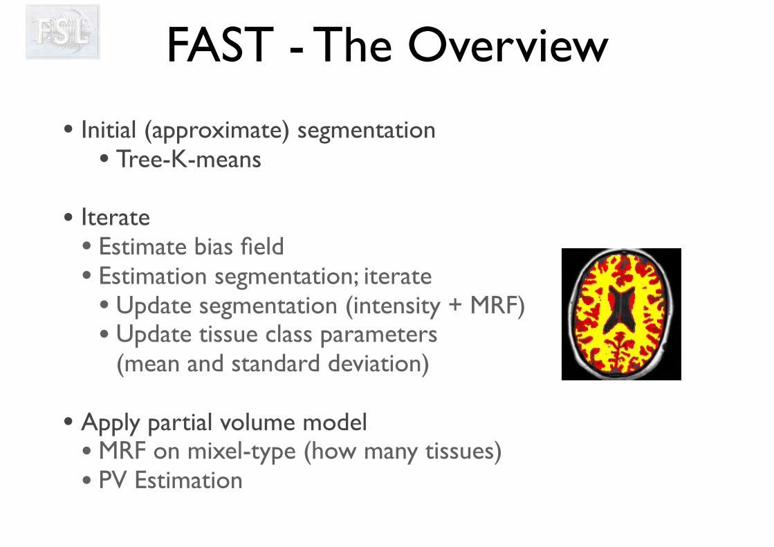
FAST - The Overview

• Initial (approximate) segmentation • Tree-K-means

• Iterate• Estimate bias field• Estimation segmentation; iterate• Update segmentation (intensity + MRF)• Update tissue class parameters

(mean and standard deviation)

• Apply partial volume model• MRF on mixel-type (how many tissues) • PV Estimation

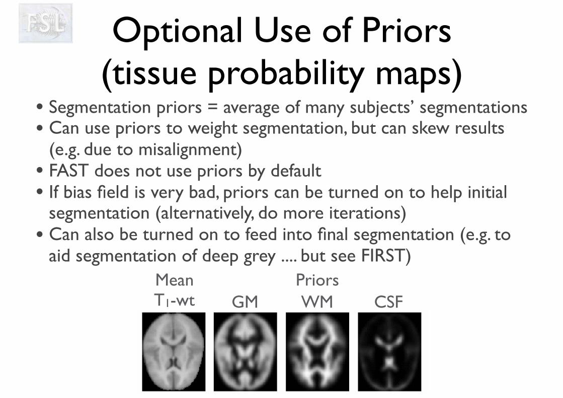
Optional Use of Priors (tissue probability maps)

• Segmentation priors = average of many subjects’ segmentations• Can use priors to weight segmentation, but can skew results

(e.g. due to misalignment)• FAST does not use priors by default• If bias field is very bad, priors can be turned on to help initial

segmentation (alternatively, do more iterations)• Can also be turned on to feed into final segmentation (e.g. to

aid segmentation of deep grey .... but see FIRST)Priors

GM WM CSFMeanT1-wt

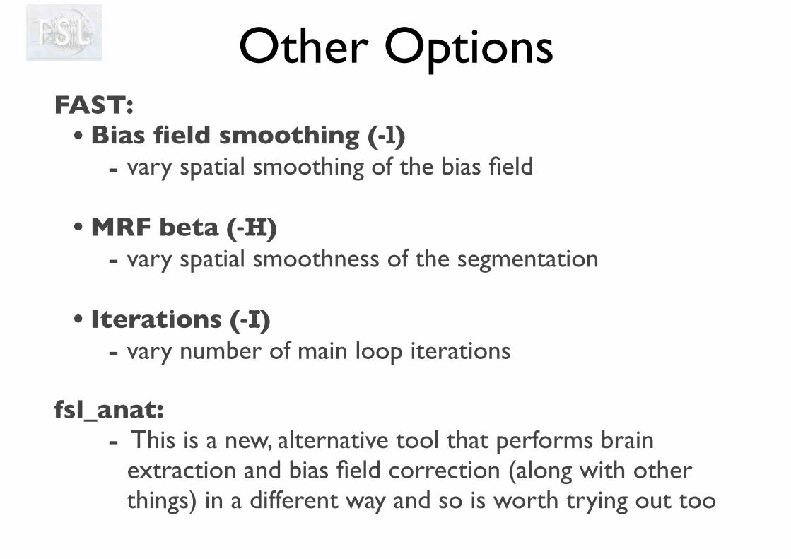
Other OptionsFAST:

• Bias field smoothing (-l) - vary spatial smoothing of the bias field

• MRF beta (-H)- vary spatial smoothness of the segmentation

• Iterations (-I)- vary number of main loop iterations

fsl_anat:- This is a new, alternative tool that performs brain

extraction and bias field correction (along with other things) in a different way and so is worth trying out too

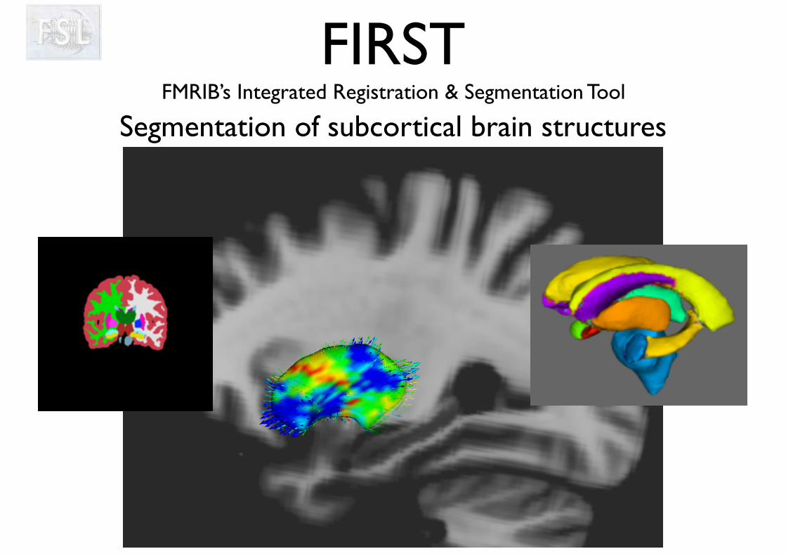
FIRST FMRIB’s Integrated Registration & Segmentation Tool

Segmentation of subcortical brain structures

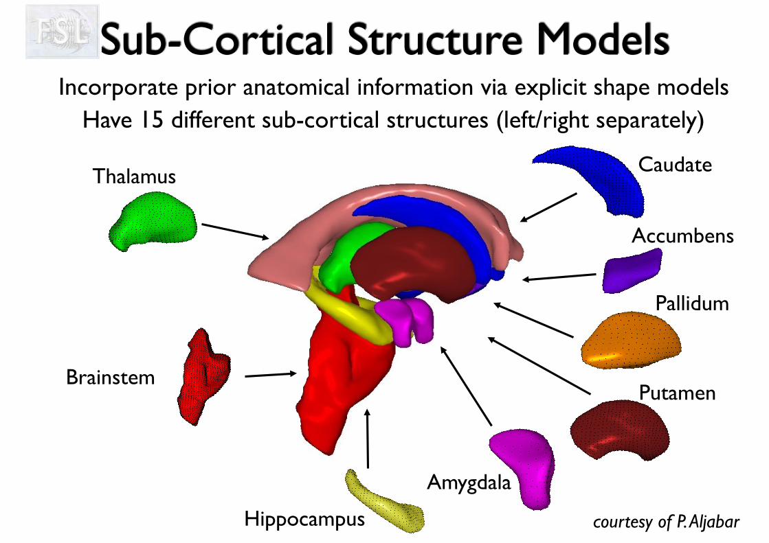
Sub-Cortical Structure Models

courtesy of P. Aljabar

Thalamus

Brainstem

Hippocampus

Amygdala

Caudate

Pallidum

Putamen

Accumbens

• Incorporate prior anatomical information via explicit shape models• Have 15 different sub-cortical structures (left/right separately)

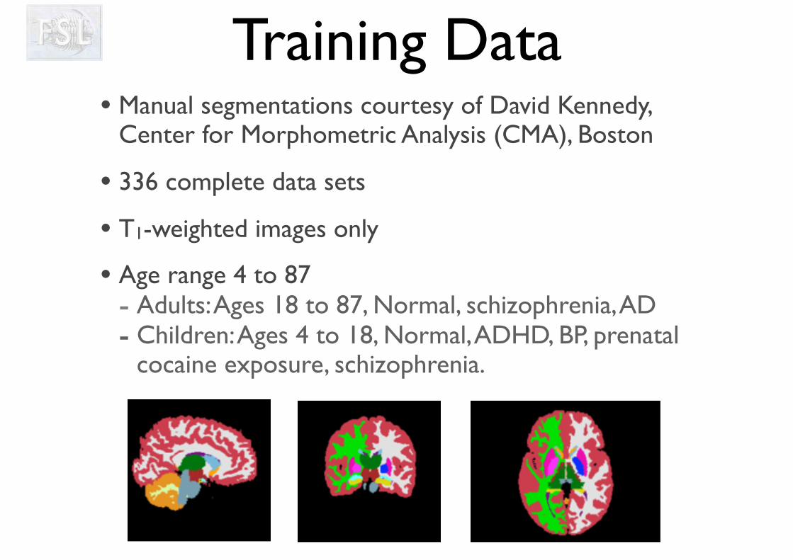
Training Data• Manual segmentations courtesy of David Kennedy,

Center for Morphometric Analysis (CMA), Boston

• 336 complete data sets

• T1-weighted images only

• Age range 4 to 87- Adults: Ages 18 to 87, Normal, schizophrenia, AD- Children: Ages 4 to 18, Normal, ADHD, BP, prenatal

cocaine exposure, schizophrenia.

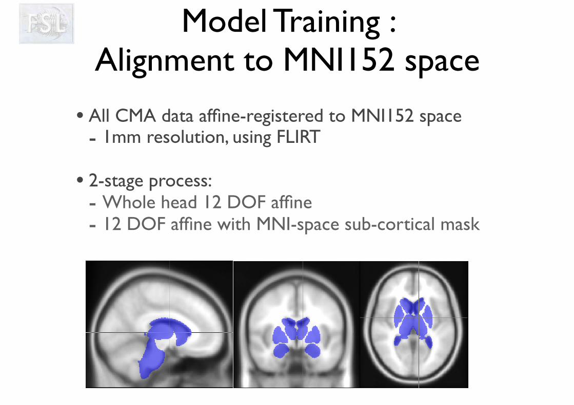
Model Training : Alignment to MNI152 space

• All CMA data affine-registered to MNI152 space- 1mm resolution, using FLIRT

• 2-stage process:- Whole head 12 DOF affine- 12 DOF affine with MNI-space sub-cortical mask

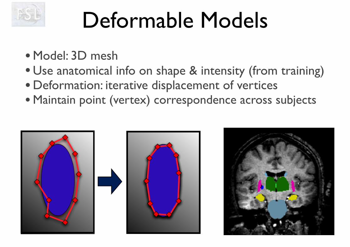
• Model: 3D mesh• Use anatomical info on shape & intensity (from training)• Deformation: iterative displacement of vertices• Maintain point (vertex) correspondence across subjects

Deformable Models

• Model average shape (from vertex locations)

• Also model/learn likely variations about this mean - modes of variation of the population; c.f. PCA- also call eigenvectors

• Average shape and the modes of variation serve as prior information (known before seeing the new image that is to be segmented)- formally it uses a Bayesian formulation

The Model: Shape

The Model: Shape

€

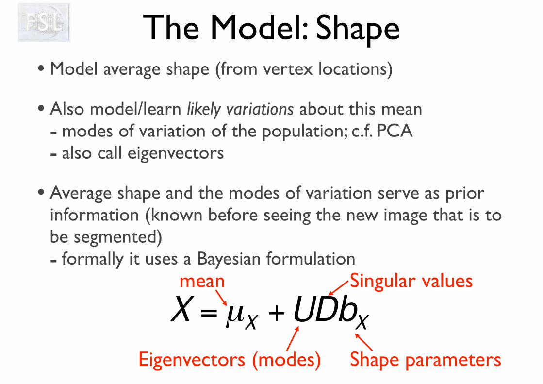
X = µX +UDbXmean

Eigenvectors (modes)

Singular values

Shape parameters

• Model average shape (from vertex locations)

• Also model/learn likely variations about this mean - modes of variation of the population; c.f. PCA- also call eigenvectors

• Average shape and the modes of variation serve as prior information (known before seeing the new image that is to be segmented)- formally it uses a Bayesian formulation

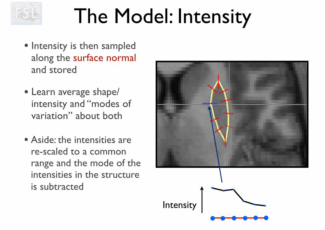
• Intensity is then sampled along the surface normal and stored

• Learn average shape/intensity and “modes of variation” about both

• Aside: the intensities are re-scaled to a common range and the mode of the intensities in the structure is subtracted

The Model: Intensity

Intensity

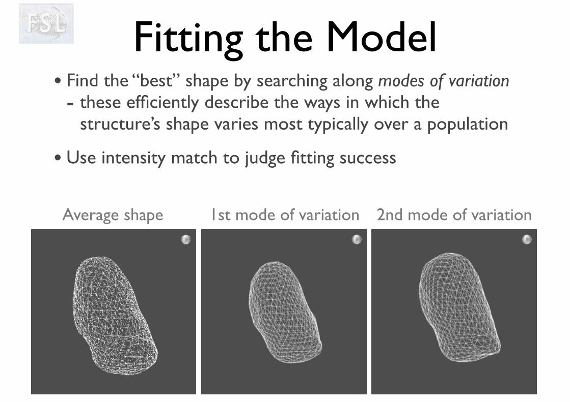
Fitting the Model• Find the “best” shape by searching along modes of variation - these efficiently describe the ways in which the

structure’s shape varies most typically over a population

• Use intensity match to judge fitting success

1st mode of variation 2nd mode of variationAverage shape

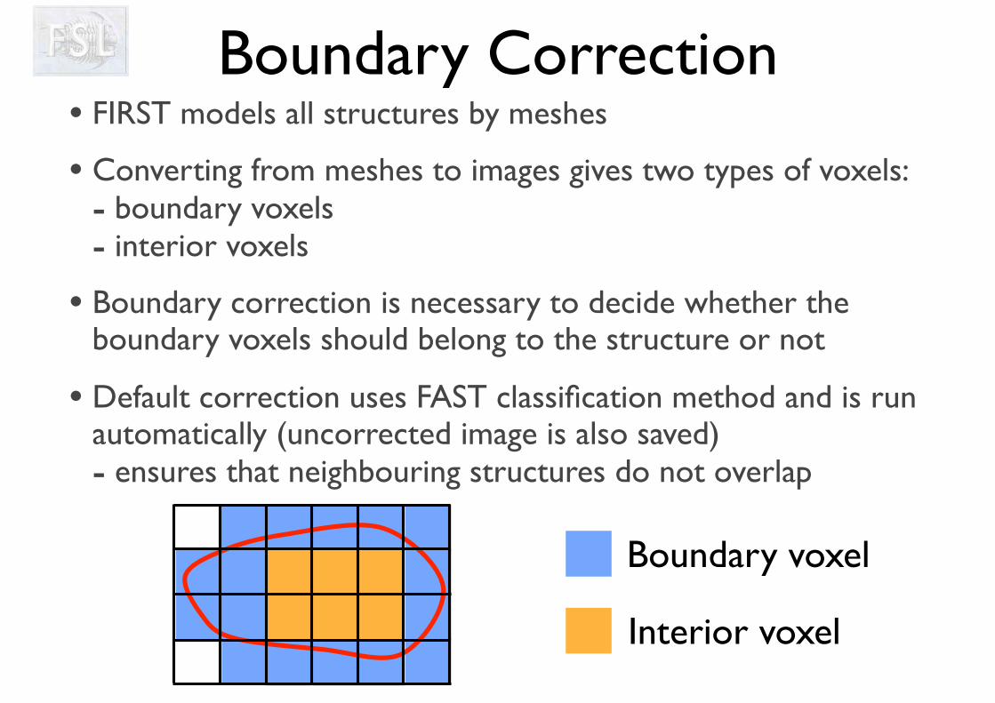
Boundary Correction

Boundary voxel

Interior voxel

• FIRST models all structures by meshes

• Converting from meshes to images gives two types of voxels:- boundary voxels- interior voxels

• Boundary correction is necessary to decide whether the boundary voxels should belong to the structure or not

• Default correction uses FAST classification method and is run automatically (uncorrected image is also saved)- ensures that neighbouring structures do not overlap

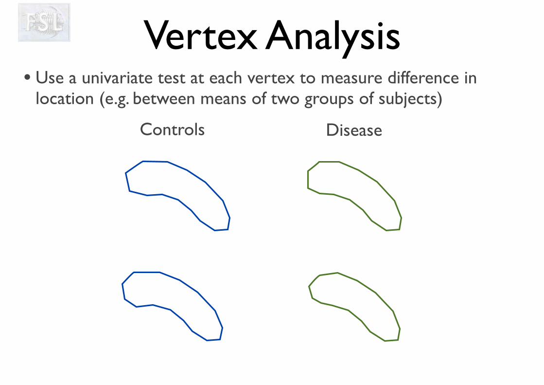
Vertex Analysis• Use a univariate test at each vertex to measure difference in

location (e.g. between means of two groups of subjects)

Controls Disease

Vertex Analysis• Use a univariate test at each vertex to measure difference in

location (e.g. between means of two groups of subjects)

Controls Disease

Consider each vertex in turn

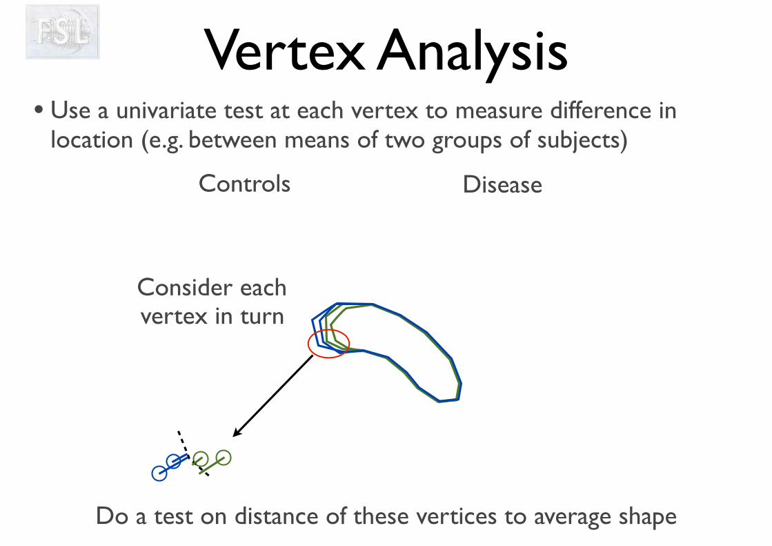
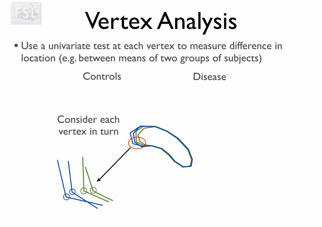
Vertex Analysis• Use a univariate test at each vertex to measure difference in

location (e.g. between means of two groups of subjects)

Controls Disease

Do a test on distance of these vertices to average shape

Consider each vertex in turn

Vertex Analysis

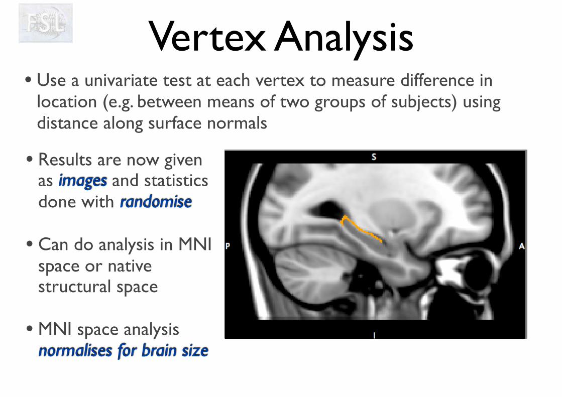
• Results are now given as images and statistics done with randomise

• Can do analysis in MNI space or native structural space

• MNI space analysis normalises for brain size

• Use a univariate test at each vertex to measure difference in location (e.g. between means of two groups of subjects) using distance along surface normals

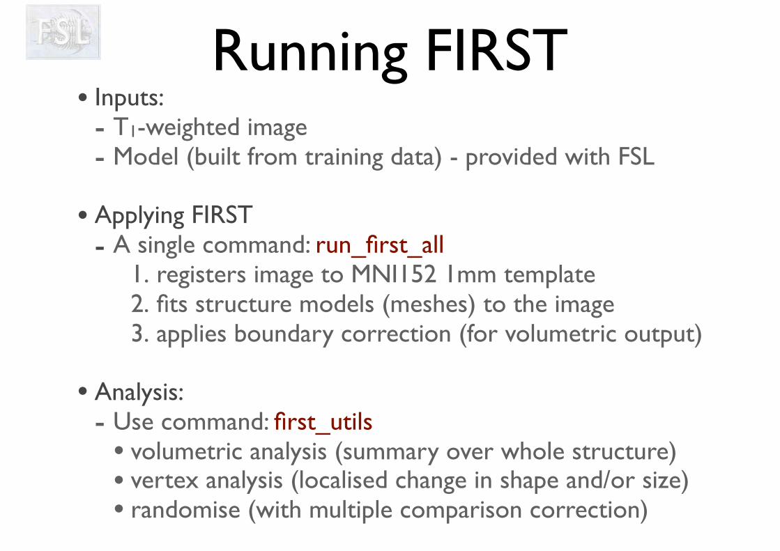
Running FIRST • Inputs: - T1-weighted image- Model (built from training data) - provided with FSL

• Applying FIRST- A single command: run_first_all

1. registers image to MNI152 1mm template 2. fits structure models (meshes) to the image3. applies boundary correction (for volumetric output)

• Analysis:- Use command: first_utils

• volumetric analysis (summary over whole structure)• vertex analysis (localised change in shape and/or size)• randomise (with multiple comparison correction)

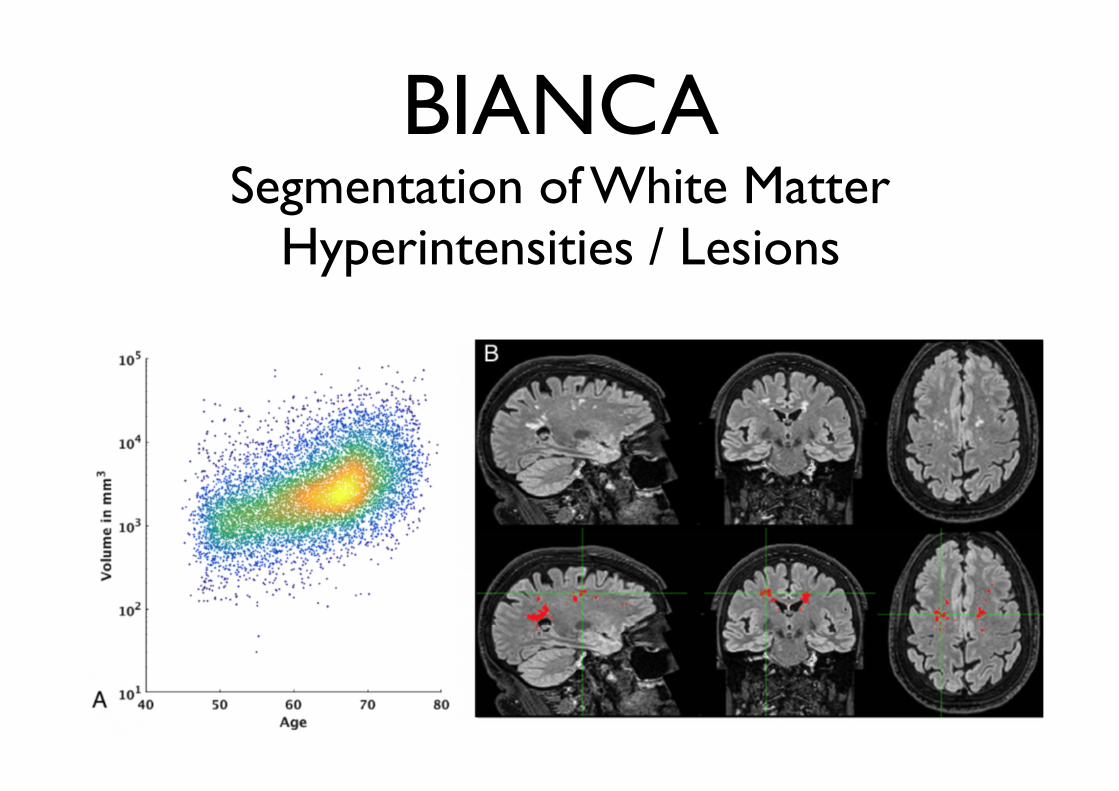
BIANCASegmentation of White Matter

Hyperintensities / Lesions

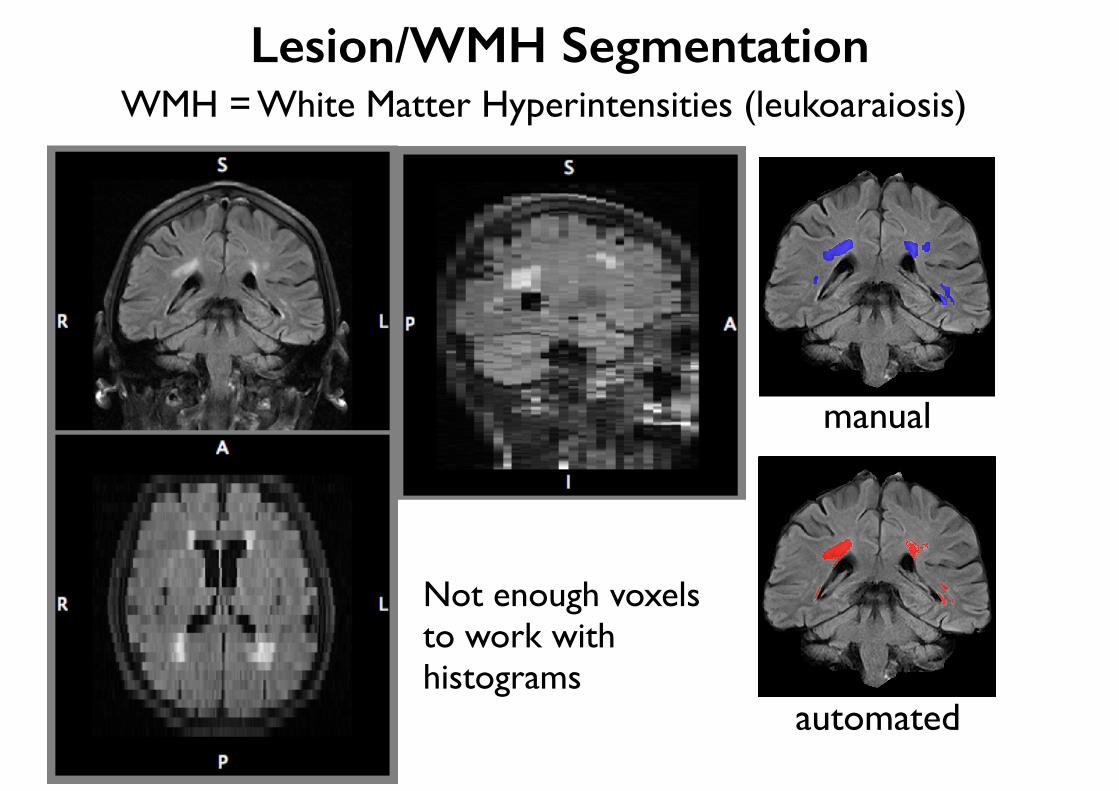
Lesion/WMH SegmentationWMH = White Matter Hyperintensities (leukoaraiosis)

manual

automated

Not enough voxels to work with histograms

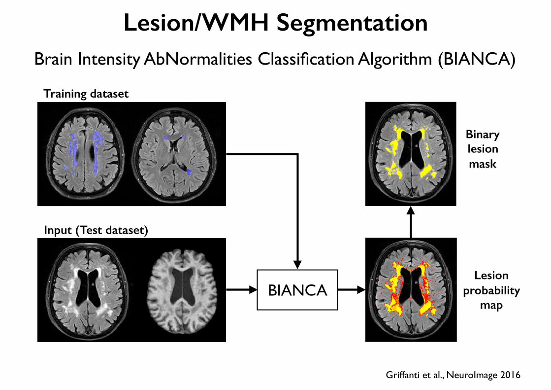
Brain Intensity AbNormalities Classification Algorithm (BIANCA)

Griffanti et al., NeuroImage 2016

Multimodal

Supervised

BIANCA

Training dataset

Input (Test dataset)

Lesion probability

map

Binary lesion mask

Lesion/WMH Segmentation

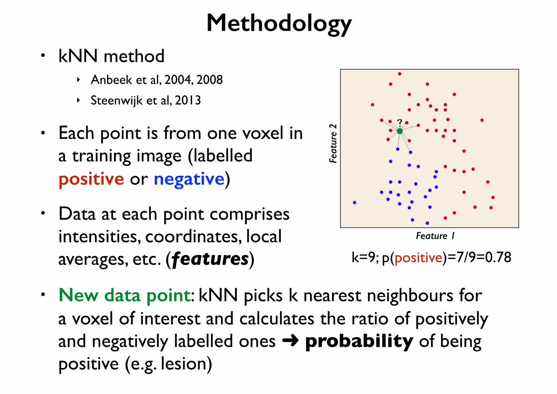
Methodology• kNN method

‣ Anbeek et al, 2004, 2008 ‣ Steenwijk et al, 2013

• Each point is from one voxel in a training image (labelled positive or negative)

• New data point: kNN picks k nearest neighbours for a voxel of interest and calculates the ratio of positively and negatively labelled ones ➜ probability of being positive (e.g. lesion)

Feature 1

Feat

ure

2

• Data at each point comprises intensities, coordinates, local averages, etc. (features) k=9; p(positive)=7/9=0.78

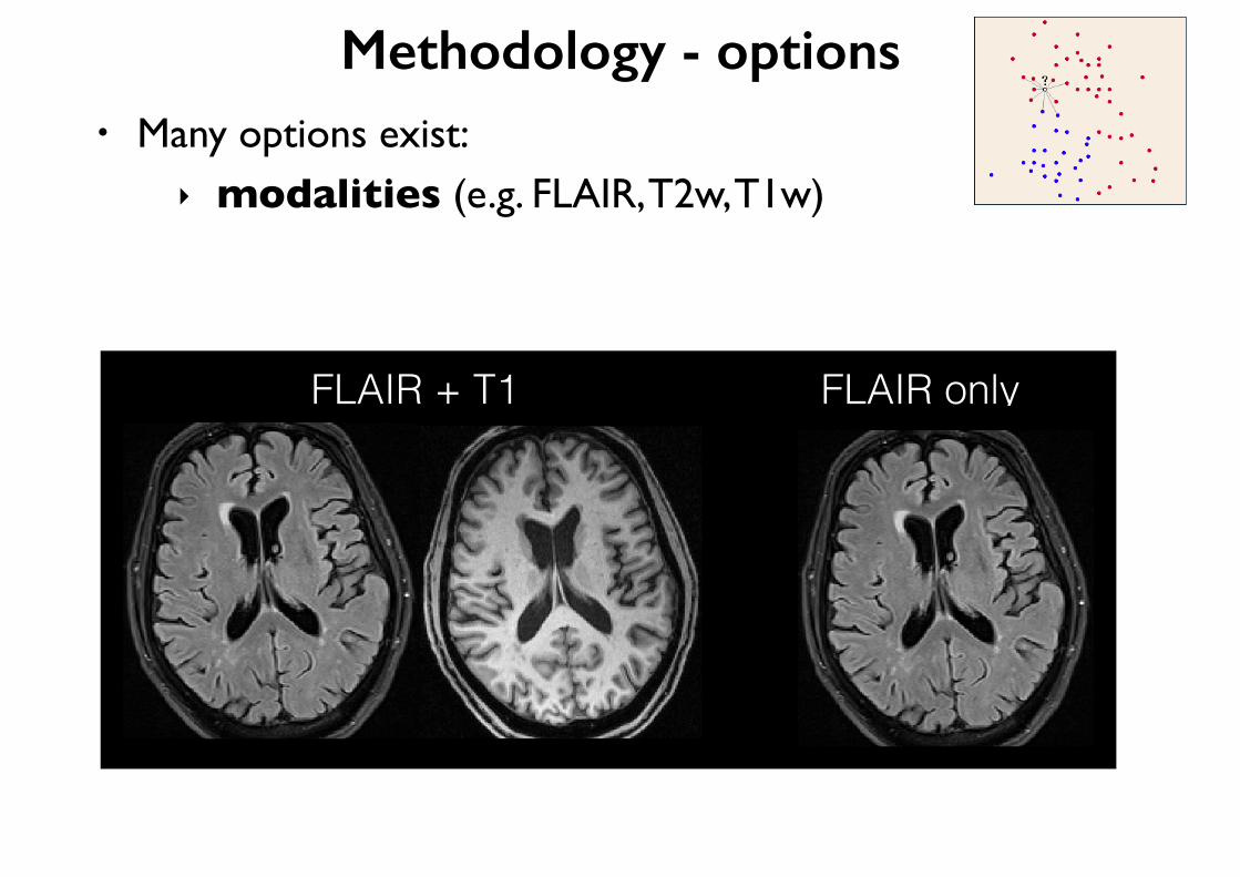
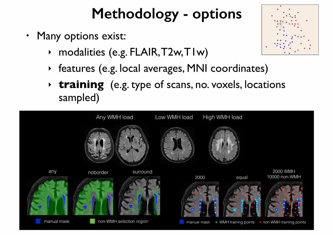
Methodology - options• Many options exist:

‣ modalities (e.g. FLAIR, T2w, T1w)‣ features (e.g. local averages, MNI coordinates)‣ training (e.g. type of scans, no. voxels, locations

sampled)‣ post-processing (e.g. masking / thresholding)‣ choice of classifier (e.g. RF, NN, SVM, Adaboost)

FLAIR + T1 FLAIR only

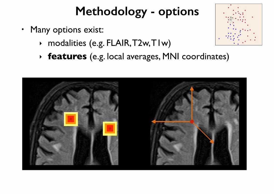
• Many options exist:‣ modalities (e.g. FLAIR, T2w, T1w)‣ features (e.g. local averages, MNI coordinates)‣ training (e.g. type of scans, no. voxels, locations

sampled)‣ post-processing (e.g. masking / thresholding)‣ choice of classifier (e.g. RF, NN, SVM, Adaboost)

Methodology - options

• Many options exist:‣ modalities (e.g. FLAIR, T2w, T1w)‣ features (e.g. local averages, MNI coordinates)‣ training (e.g. type of scans, no. voxels, locations

sampled)‣ post-processing (e.g. masking / thresholding)‣ choice of classifier (e.g. RF, NN, SVM, Adaboost)

Methodology - options

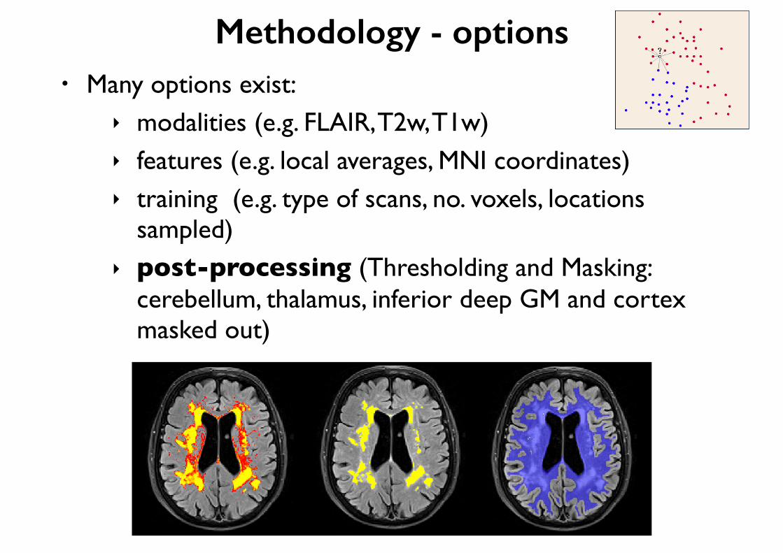
• Many options exist:‣ modalities (e.g. FLAIR, T2w, T1w)‣ features (e.g. local averages, MNI coordinates)‣ training (e.g. type of scans, no. voxels, locations

sampled)‣ post-processing (Thresholding and Masking:

cerebellum, thalamus, inferior deep GM and cortex masked out)

Methodology - options

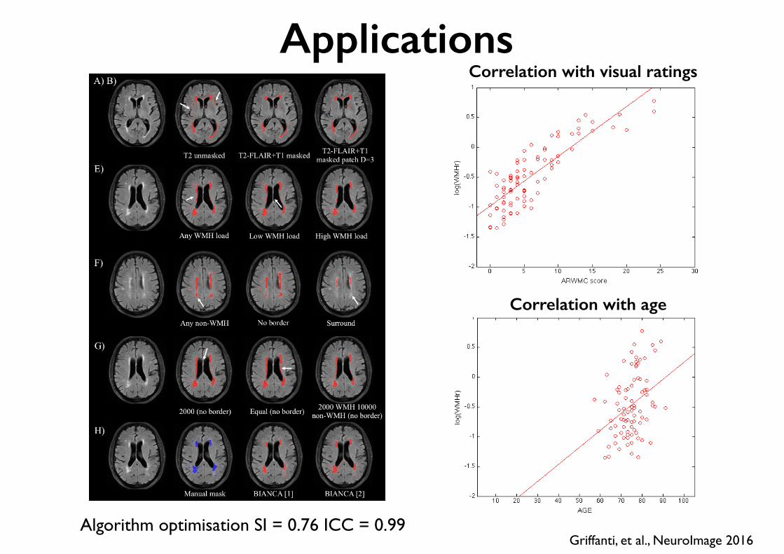
Applications

Griffanti, et al., NeuroImage 2016Algorithm optimisation SI = 0.76 ICC = 0.99

Correlation with visual ratings

Correlation with age

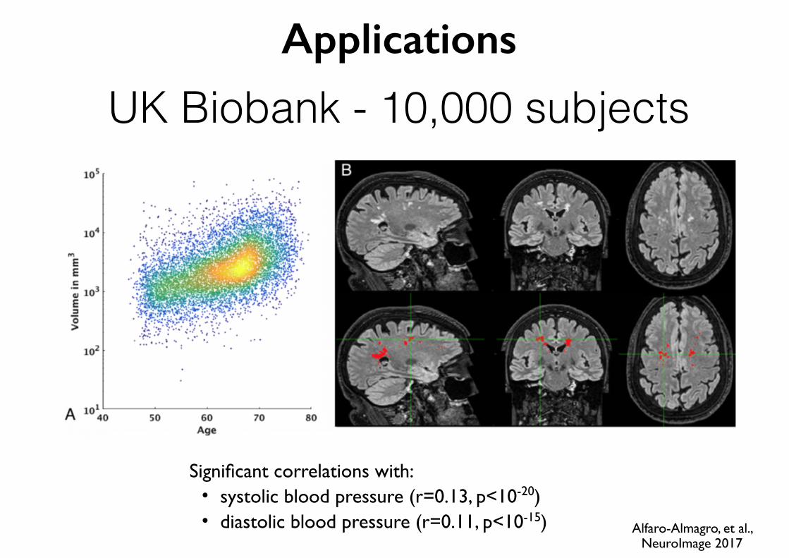
UK Biobank - 10,000 subjects

Significant correlations with:• systolic blood pressure (r=0.13, p<10-20)• diastolic blood pressure (r=0.11, p<10-15) Alfaro-Almagro, et al.,

NeuroImage 2017

Applications

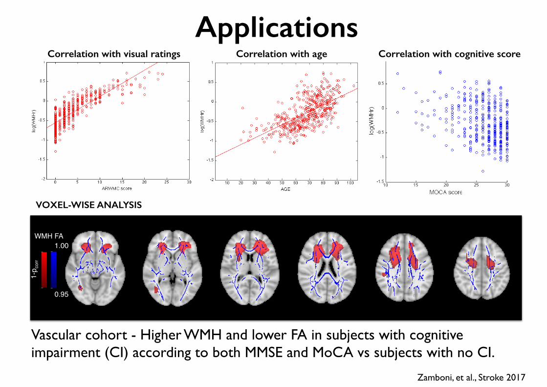
Vascular cohort - Higher WMH and lower FA in subjects with cognitive impairment (CI) according to both MMSE and MoCA vs subjects with no CI.

1-p c

orr!

1.00!

0.95!

WMH FA!

Correlation with visual ratings Correlation with age Correlation with cognitive score

Applications

Zamboni, et al., Stroke 2017

VOXEL-WISE ANALYSIS

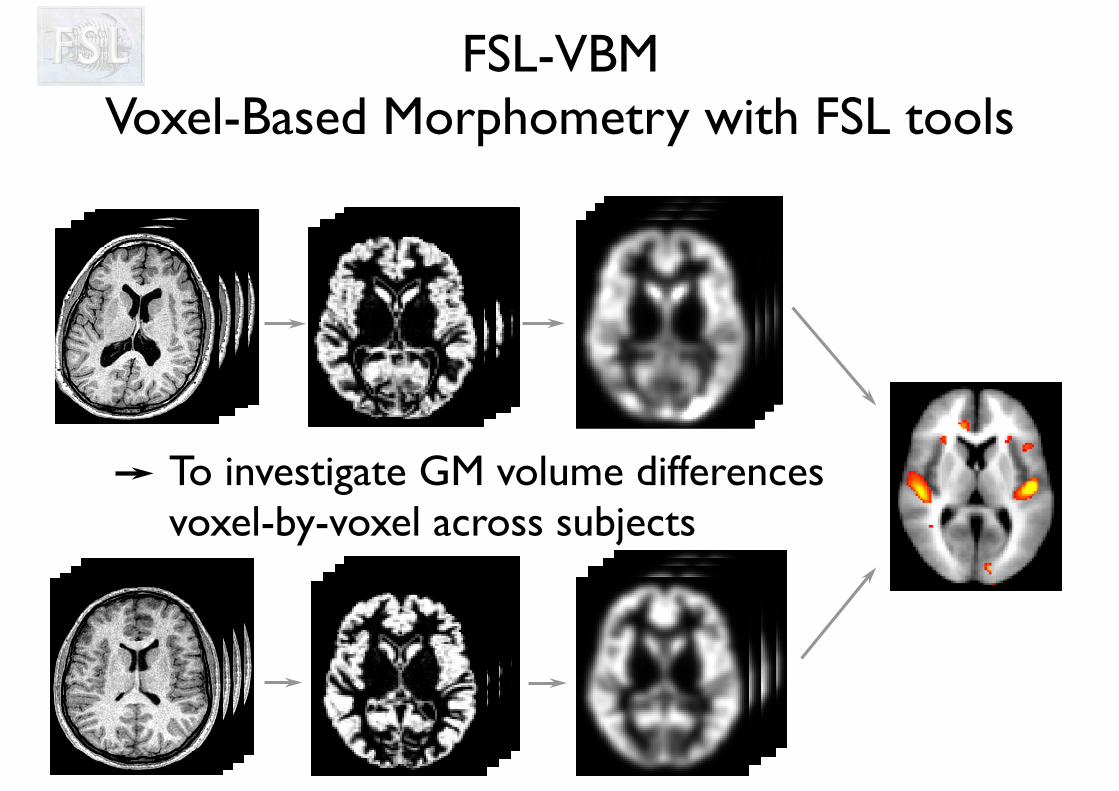
FSL-VBM Voxel-Based Morphometry with FSL tools

To investigate GM volume differences voxel-by-voxel across subjects

Voxel-based analysis of local GM volume

• Somewhat controversial approach (e.g. what exactly is it “looking at”?)

• BUT - it gives some clues for: - volume/gyrification differences between populations - correlations with (e.g.) clinical score - fMRI/PET results “caused” by structural changes

• Currently it is very widely used, although some other alternatives exist

(e.g. surface-based thickness analysis, tensor/deformation-based morphometry)

• No a priori required = whole-brain unbiased analysis• Automated = Reproducible intra/inter-rater • Quick

• Localisation of the GM differences across subjects ⇒ non-linear registration

• Trade-off: - not enough non-linear = no correspondence - too much non-linear = no difference (in intensities)

Voxel-based analysis of local GM volume

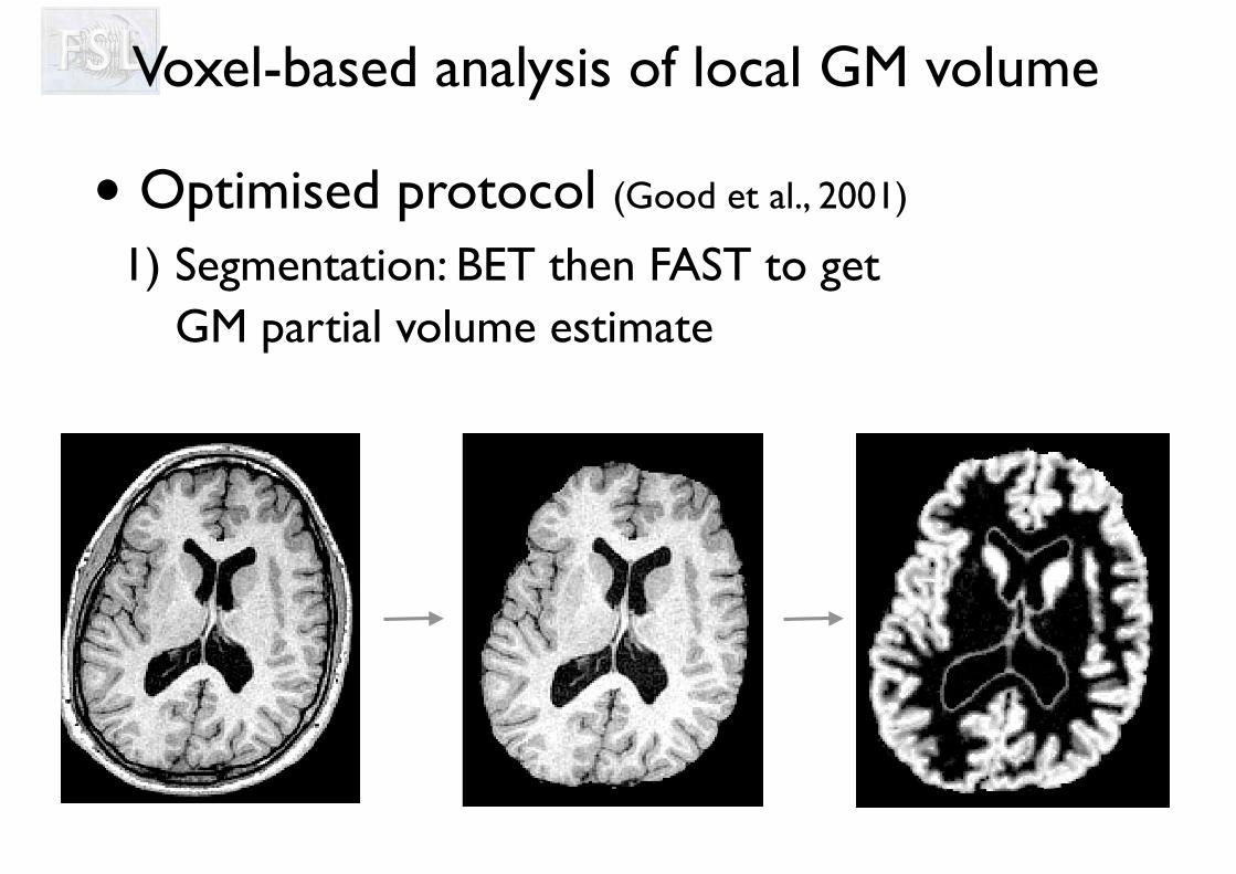
• Optimised protocol (Good et al., 2001)

Voxel-based analysis of local GM volume

1) Segmentation: BET then FAST to get GM partial volume estimate

X patients X controls

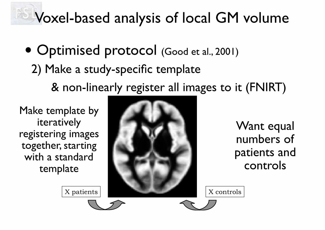
• Optimised protocol (Good et al., 2001)

2) Make a study-specific template & non-linearly register all images to it (FNIRT)

Want equal numbers of patients and

controls

Make template by iteratively

registering images together, starting with a standard

template

Voxel-based analysis of local GM volume

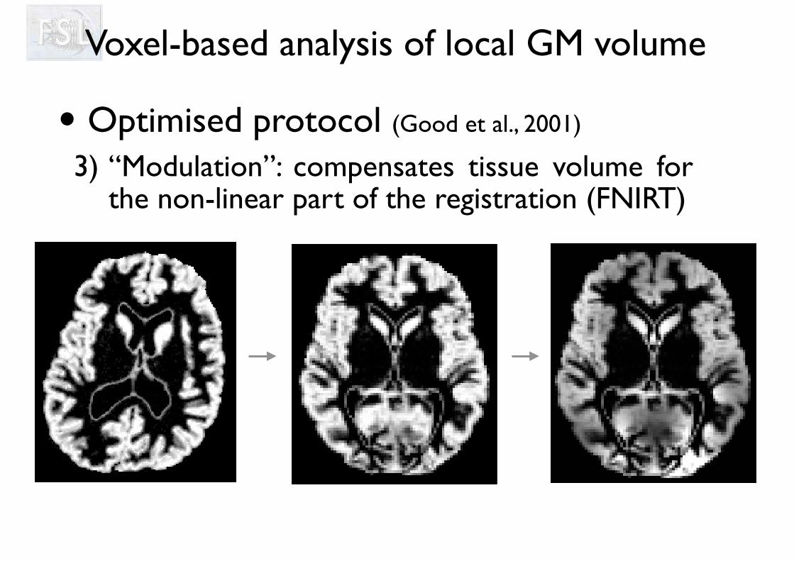
• Optimised protocol (Good et al., 2001)

3) “Modulation”: compensates tissue volume for the non-linear part of the registration (FNIRT)

Voxel-based analysis of local GM volume

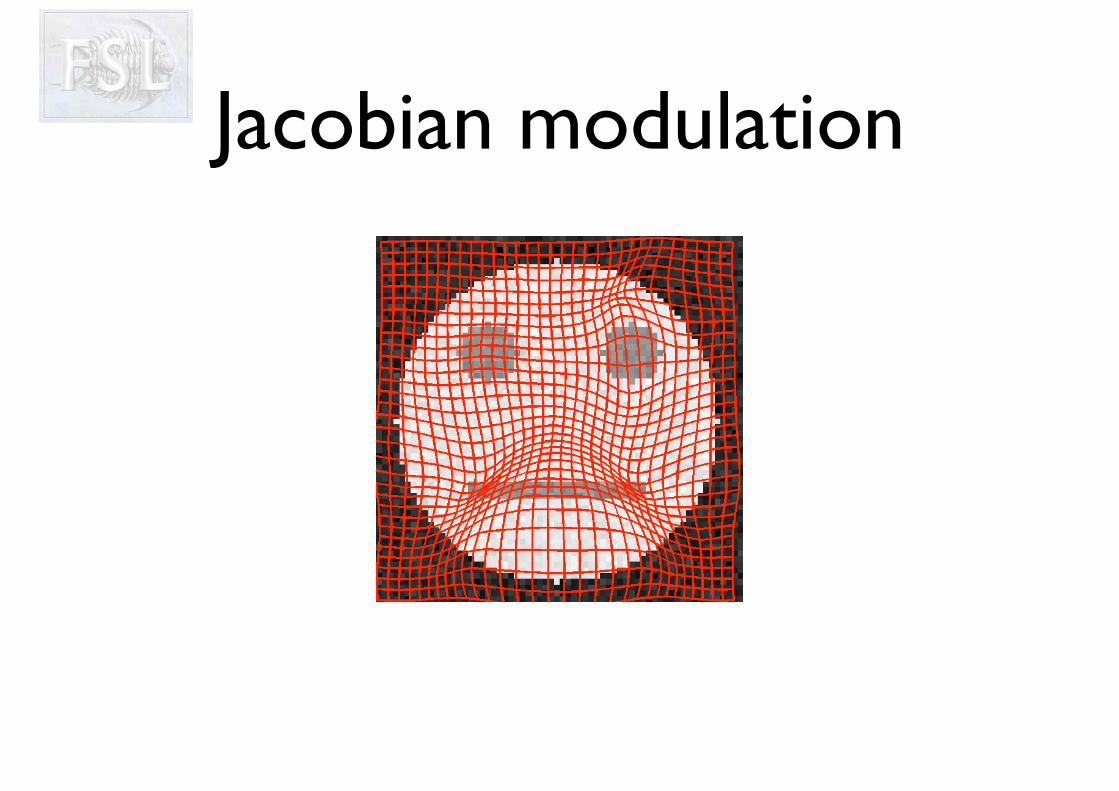
Jacobian modulation

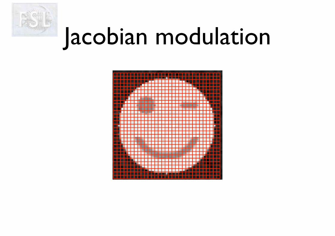
Jacobian modulation

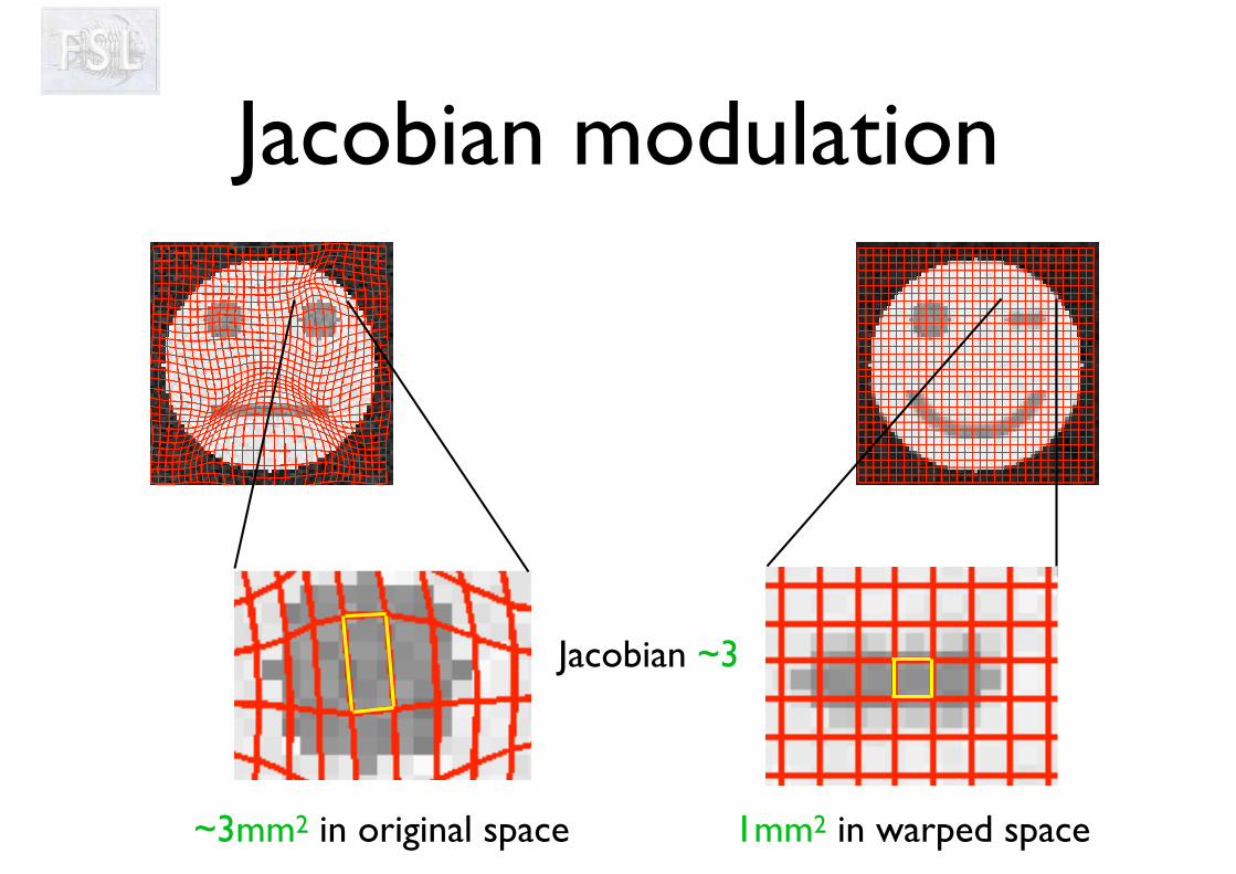
~3mm2 in original space 1mm2 in warped space

Jacobian ~3

Jacobian modulation

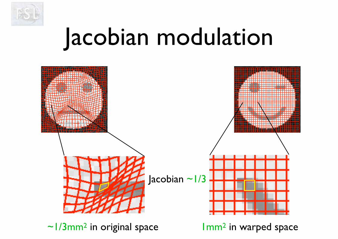
~1/3mm2 in original space 1mm2 in warped space

Jacobian ~1/3

Jacobian modulation

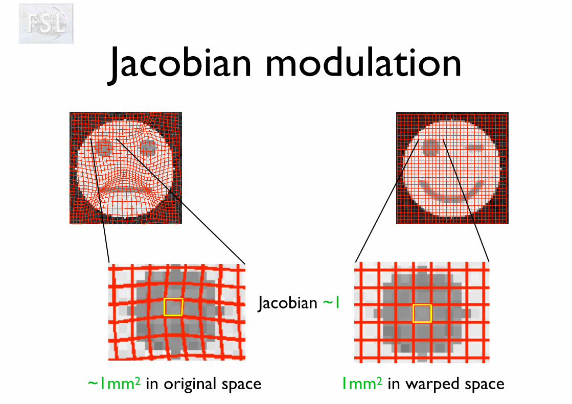
~1mm2 in original space 1mm2 in warped space

Jacobian ~1

Jacobian modulation

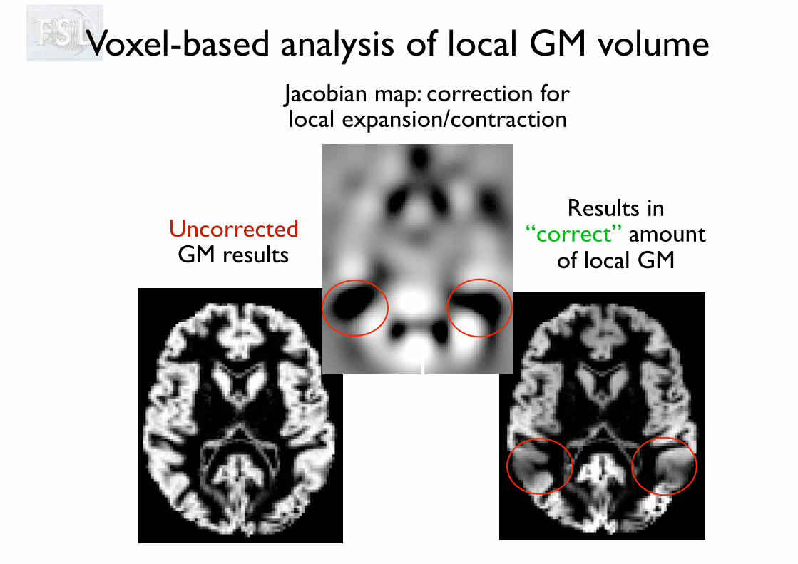
Jacobian map: correction for local expansion/contraction

Results in “correct” amount

of local GMUncorrected GM results

Voxel-based analysis of local GM volume

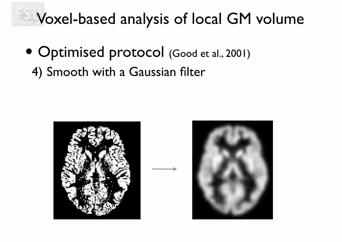
• Optimised protocol (Good et al., 2001)

4) Smooth with a Gaussian filter

Voxel-based analysis of local GM volume

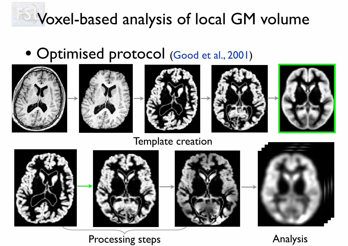
AnalysisProcessing steps

• Optimised protocol (Good et al., 2001)

Template creation

Voxel-based analysis of local GM volume

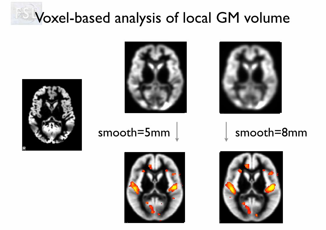
smooth=5mm smooth=8mm

Voxel-based analysis of local GM volume

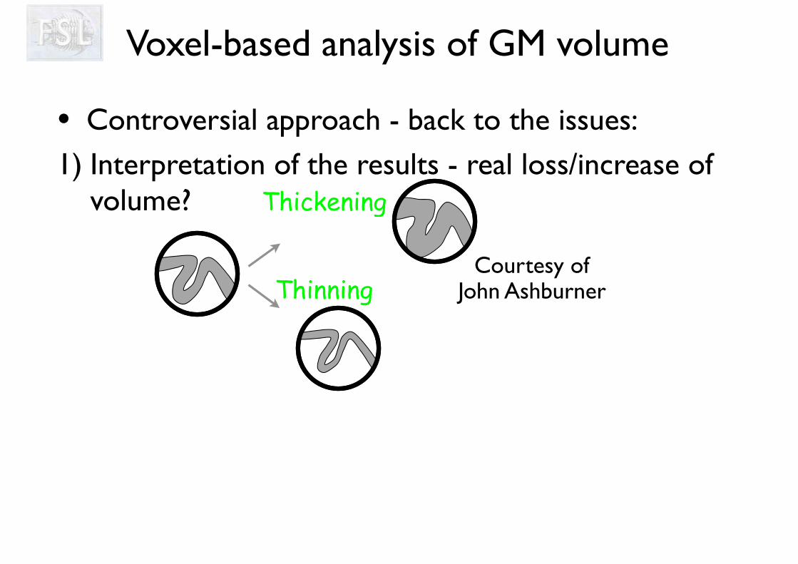
• Controversial approach - back to the issues: 1) Interpretation of the results - real loss/increase of

volume? Thickening

Thinning

Voxel-based analysis of GM volume

Courtesy ofJohn Ashburner

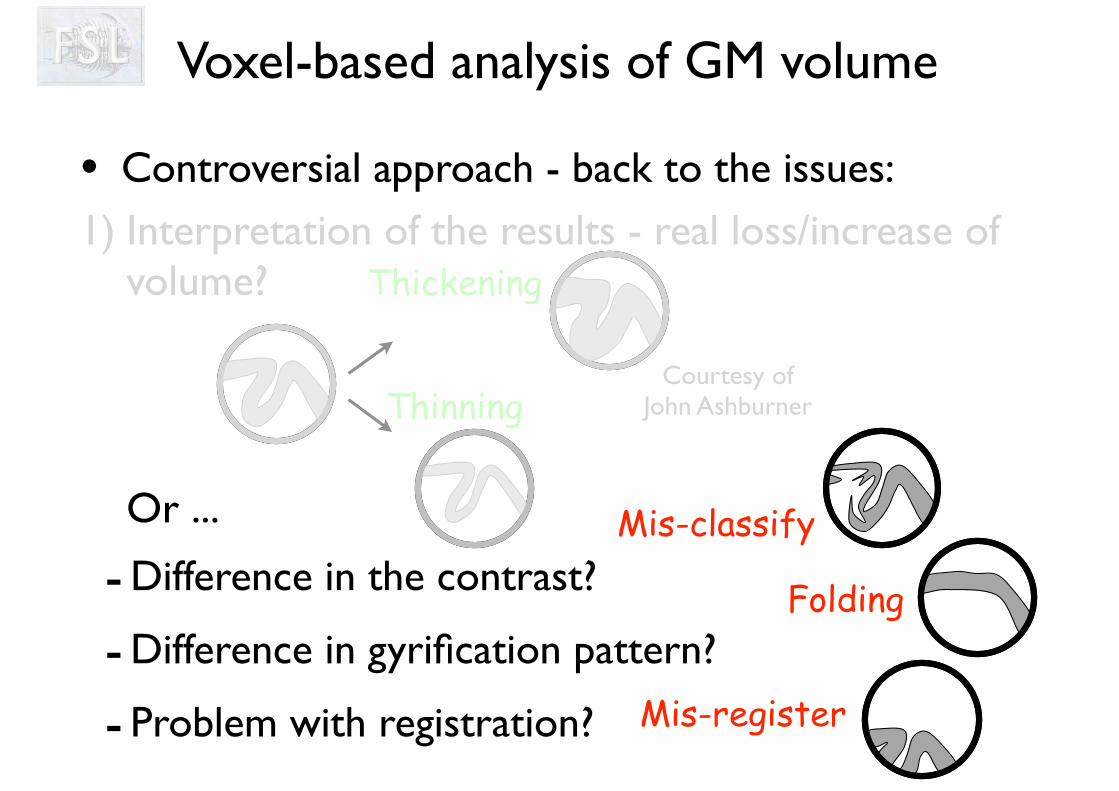
• Controversial approach - back to the issues: 1) Interpretation of the results - real loss/increase of

volume?

Or ...

- Difference in the contrast?

- Difference in gyrification pattern?

- Problem with registration?

Folding

Mis-classify

Mis-register

Courtesy ofJohn Ashburner

Thickening

Thinning

Voxel-based analysis of GM volume

Voxel-based analysis of GM volume

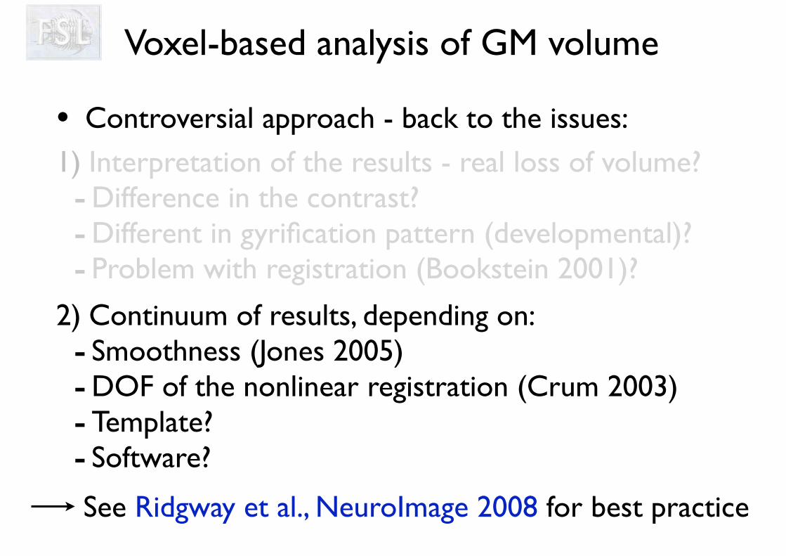
• Controversial approach - back to the issues: 1) Interpretation of the results - real loss of volume?- Difference in the contrast?- Different in gyrification pattern (developmental)?- Problem with registration (Bookstein 2001)?

2) Continuum of results, depending on:- Smoothness (Jones 2005)- DOF of the nonlinear registration (Crum 2003)- Template?- Software?

See Ridgway et al., NeuroImage 2008 for best practice

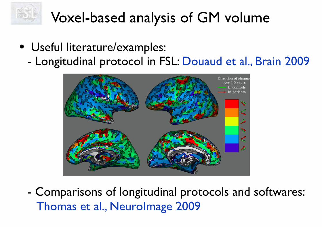
Voxel-based analysis of GM volume

• Useful literature/examples: - Longitudinal protocol in FSL: Douaud et al., Brain 2009 - Comparisons of longitudinal protocols and softwares: Thomas et al., NeuroImage 2009

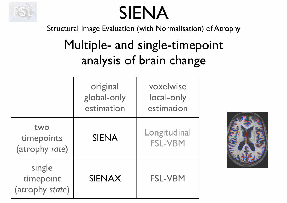
SIENA Structural Image Evaluation (with Normalisation) of Atrophy

Multiple- and single-timepoint analysis of brain change

originalglobal-onlyestimation

voxelwise local-only estimation

twotimepoints

(atrophy rate)SIENA Longitudinal

FSL-VBM

singletimepoint

(atrophy state)SIENAX FSL-VBM

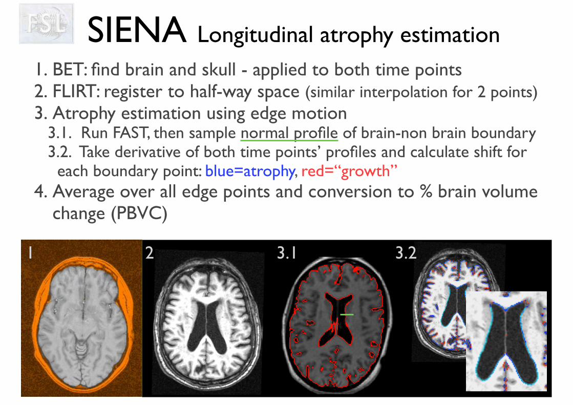
SIENA Longitudinal atrophy estimation1. BET: find brain and skull - applied to both time points2. FLIRT: register to half-way space (similar interpolation for 2 points)3. Atrophy estimation using edge motion

3.1. Run FAST, then sample normal profile of brain-non brain boundary3.2. Take derivative of both time points’ profiles and calculate shift for

each boundary point: blue=atrophy, red=“growth”4. Average over all edge points and conversion to % brain volume

change (PBVC)

1 2 3.1 3.2

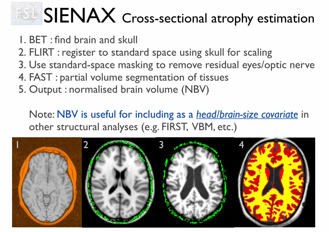
SIENAX Cross-sectional atrophy estimation

1. BET : find brain and skull2. FLIRT : register to standard space using skull for scaling3. Use standard-space masking to remove residual eyes/optic nerve4. FAST : partial volume segmentation of tissues5. Output : normalised brain volume (NBV)

Note: NBV is useful for including as a head/brain-size covariate in other structural analyses (e.g. FIRST, VBM, etc.)

1 2 3 4

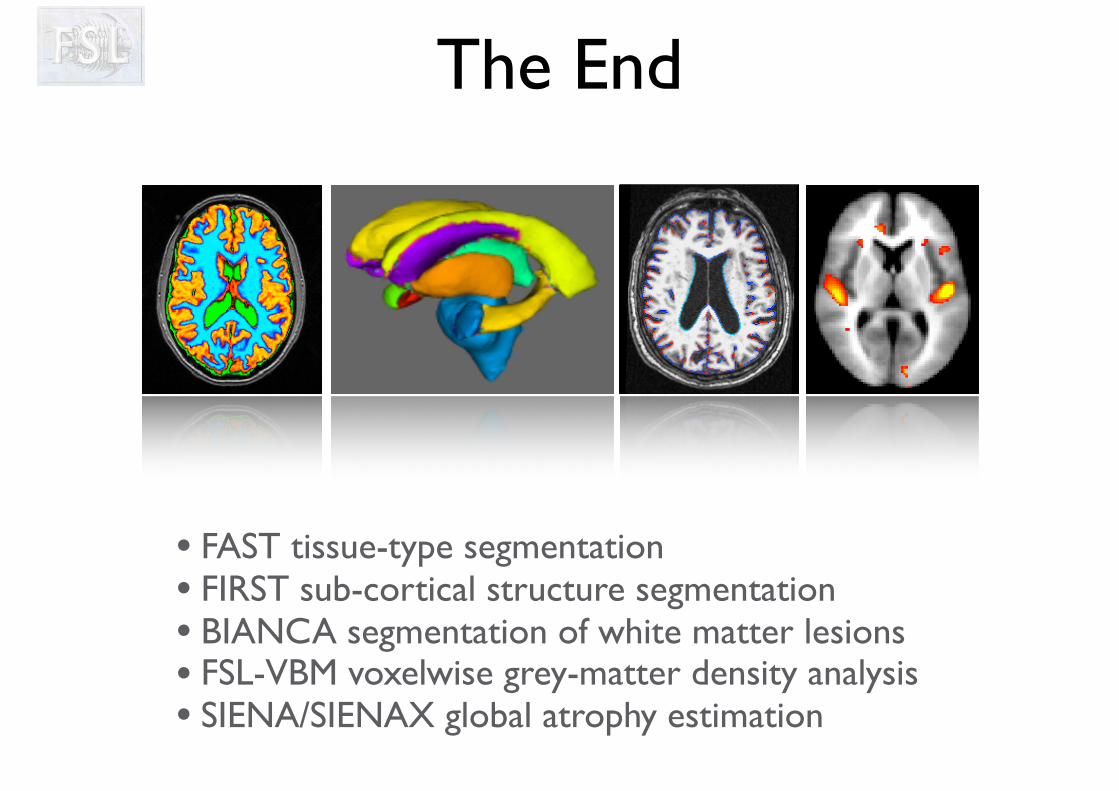
The End

• FAST tissue-type segmentation• FIRST sub-cortical structure segmentation• BIANCA segmentation of white matter lesions• FSL-VBM voxelwise grey-matter density analysis• SIENA/SIENAX global atrophy estimation