1D model for the dynamics and expansionof elongated Bose-Einstein condensates 1e-05

2e-05 6e-05 0.0001 0.0002 0.0006

-400 -200 0 200 400

-100

-50

0

50

100

Pietro Massignan and Michele Modugno

INFM - LENS - Dipartimento di Fisica, University of Florence

Via Nello Carrara 1, 50019 Sesto Fiorentino, Italy

Art. ref.: PRA 67, 023614 (2003)

Nordita

Kobenhavn, 6 March 2003

1

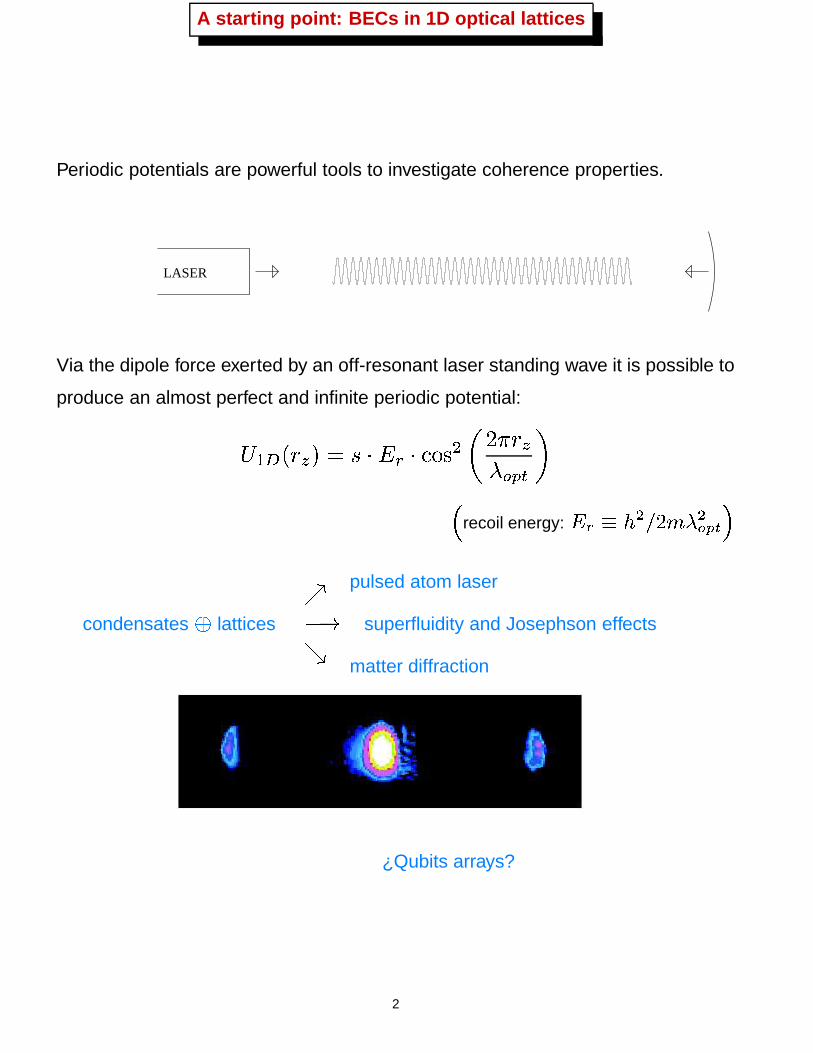
A starting point: BECs in 1D optical lattices

Periodic potentials are powerful tools to investigate coherence properties.

LASER0

10

20

30

40

50

60

70

-10 -5 0 5 10

Via the dipole force exerted by an off-resonant laser standing wave it is possible to

produce an almost perfect and infinite periodic potential:������������ ����������������� �� � "!$#&%'recoil energy: (*)*+ ,.-0/21&354.-687�9;:

pulsed atom laser

condensates < lattices superfluidity and Josephson effects

matter diffraction

= >"?@

¿Qubits arrays?

2

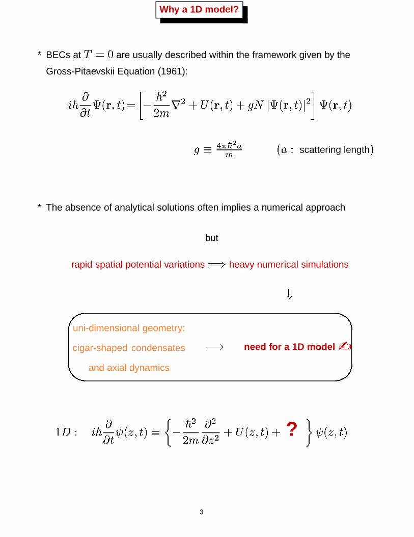
Why a 1D model?

* BECs at � �are usually described within the framework given by the

Gross-Pitaevskii Equation (1961):

�������� �� � � � � > � ���� � ��� � �� � � � � ��� � ���� � � � ��� ���� � ���� ��� "!$#% �'&)(

scattering length�

* The absence of analytical solutions often implies a numerical approach

but

rapid spatial potential variations +*

heavy numerical simulations,uni-dimensional geometry:

cigar-shaped condensates

and axial dynamics

>"?need for a 1D model ✍

-/. ( �0� �����1 �324� � �� > � ���� � �� 2 � � � �324� � � � ? 1 �324� � �

3

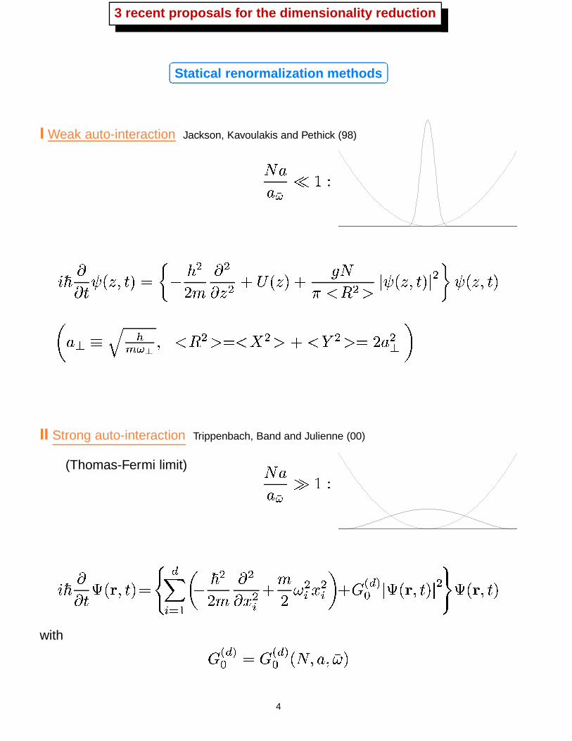
3 recent proposals for the dimensionality reduction

��

��Statical renormalization methods

I Weak auto-interaction Jackson, Kavoulakis and Pethick (98)� && �� � - (

�0�������1 �324� � �� > � ���� � �� 2 � � � �32 � � � �� �� �� � 1 �324� � � � � 1 �324� � �

& � � %���� � ��� � ��� � � ��� � � & � �

II Strong auto-interaction Trippenbach, Band and Julienne (00)

(Thomas-Fermi limit) � && �� � - (

�0���� � �� � � � �

��� �> � �� � � ���� �� � � � � �� � �� ����� �! " � ���� � � � � �' � � �

with ��� �! " �#� �! " � � �$& �%$� �4

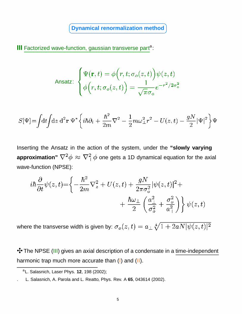
�� ��Dynamical renormalization method

III Factorized wave-function, gaussian transverse parta:

Ansatz:

��� �� ���� � � ��� � ���� ! �32 � � ��� 1 � 2 � � �� � � ���� ! �324� � � � -� � !���� � !�� ��� !������! �" #%$ #'&(# -�) �* +-,/. 910 , -1&3 2 -43 51 376 -8:9 -43 ;=< &'>?$�@ 3 A/B1 C � C - �

Inserting the Ansatz in the action of the system, under the “slowly varying

approximation” � � � D � � � �one gets a 1D dynamical equation for the axial

wave-function (NPSE):

�0���� � 1 �324� � � > � ���� � � � � �32 � � � � ����� �! � 1 �324� � � � � �� � � �� & � �

�! � �!& � � 1 �324� � �where the transverse width is given by: ! �32 � � � & � EF - � � & � � 1 �324� � � � �✣ The NPSE (III) gives an axial description of a condensate in a time-independent

harmonic trap much more accurate than (I) and (II).

aL. Salasnich, Laser Phys. 12, 198 (2002);

. L. Salasnich, A. Parola and L. Reatto, Phys. Rev. A 65, 043614 (2002).

5

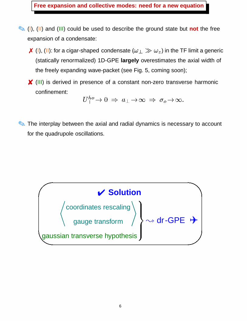
Free expansion and collective modes: need for a new equation

✎ (I), (II) and (III) could be used to describe the ground state but not the free

expansion of a condensate:

✗ (I), (II): for a cigar-shaped condensate ( � � � � ) in the TF limit a generic

(statically renormalized) 1D-GPE largely overestimates the axial width of

the freely expanding wave-packet (see Fig. 5, coming soon);

✘ (III) is derived in presence of a constant non-zero transverse harmonic

confinement: ��� !� ? � * & � ? � * ! ? � �

✎ The interplay between the axial and radial dynamics is necessary to account

for the quadrupole oscillations.

✔ Solution

coordinates rescaling

gauge transform

gaussian transverse hypothesis

�������� dr -GPE ✈

6

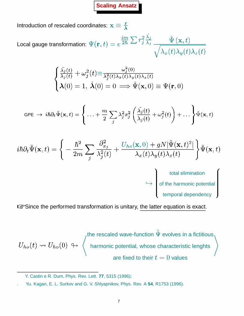
Scaling Ansatz

Introduction of rescaled coordinates: � � ��Local gauge transformation:

���� � � � � %� � � �� ����� � � � � � � � � � � � � � � � � ��� � ���� � % ��� � % � � �� � � � � � !� � " � !� � % ���� � % ���� � % ���� � % � � � � - ���� �3� � � +* � � � � � � ���� � �

GPE � ����� 9�� "!$#&%('*) + ,-/.10202043 5 6 7 8 -7�9 -7 :8 7 !$'()8 7 !$'() 3<; -7 !$'() 3�020=0?>/@A � "!$#&%('*)

�0� � % � � � � � > � ���� � � � � �� � � � � � � ! � � � � � � ��� � � � � � � � � � � � � � � � �� � � � � � � �B C

DFEEEEEEEEEEG total elimination

of the harmonic potential

temporal dependency

HEEEEEEEEEEI☞ Since the performed transformation is unitary, the latter equation is exact.

� � ! � � �KJ � � ! � � �ML the rescaled wave-function evolves in a fictitious

harmonic potential, whose characteristic lenghts

are fixed to their � �values

Y. Castin e R. Dum, Phys. Rev. Lett. 77, 5315 (1996);

. Yu. Kagan, E. L. Surkov and G. V. Shlyapnikov, Phys. Rev. A 54, R1753 (1996).

7

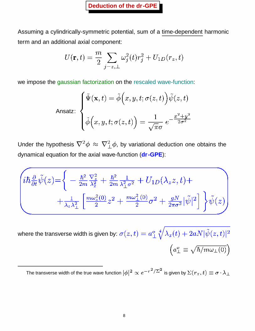
Deduction of the dr -GPE

Assuming a cylindrically-symmetric potential, sum of a time-dependent harmonic

term and an additional axial component:� ���� � � � � � � �� � � �� � � � � �� � � ��� � � � � �we impose the gaussian factorization on the rescaled wave-function:

Ansatz:

����� ���� � � � � � � � ��� � ���� �32 � � ��� 1 � 2 � � �� � ��� � ���� �324� � � � -� � � �

!�� � !��� !Under the hypothesis � � � D � � � �

, by variational deduction one obtains the

dynamical equation for the axial wave-function (dr -GPE):

��� �� '� �� ���� � � -6 5 � -�8 -� � � -6 5 �8 - 8�� - � � ��� ��� �! "�#$� �� �8 � 8 - 8 % 5 ; -� !'&�)6 6 � 5 ; -8 !'&�)6 ( 6 � )+*6�, � -.- � -

6�/ � �� ��

where the transverse width is given by: � 2 � � � & ! � E � � � � � & � � 1 �324� � � � �'10 6 8 + 2 , /&376 8 <43 @ :The transverse width of the true wave function 57685 -:9 ;=< ) !�>�? ! is given by @ !BA � %*'()DC �FE 8 8

8

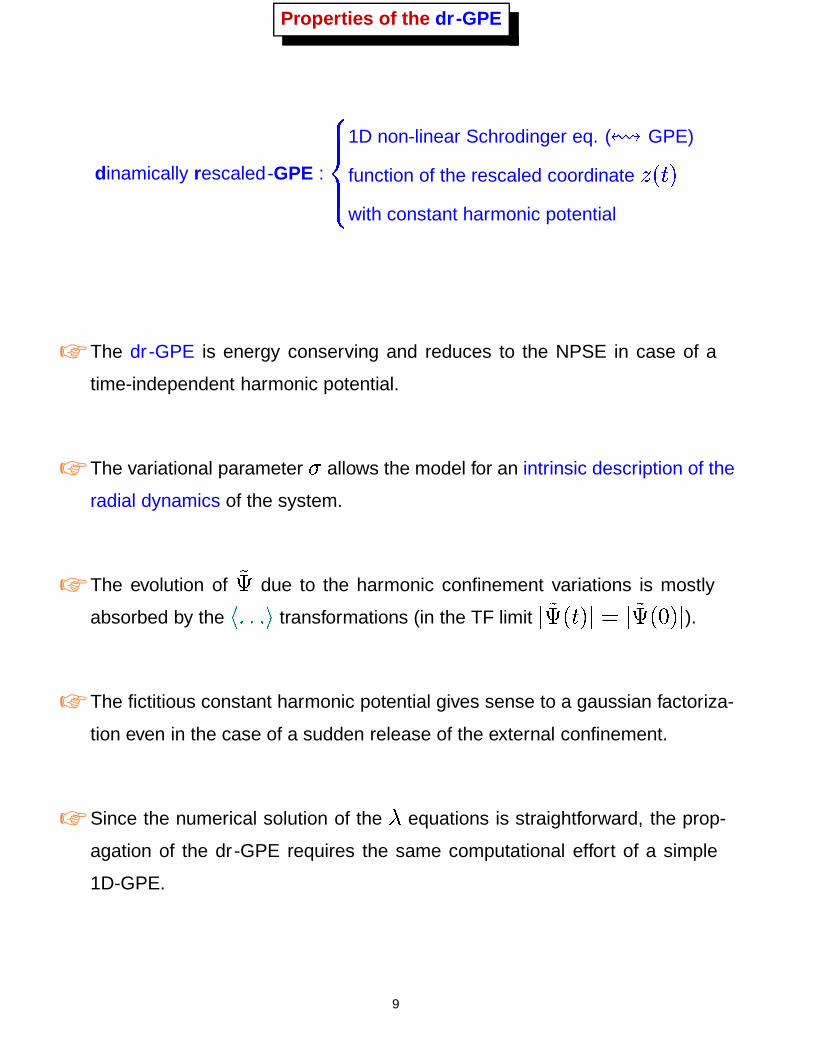
Properties of the dr -GPE

dinamically rescaled-GPE :

���� ��� 1D non-linear Schrodinger eq. ( � GPE)

function of the rescaled coordinate2 � � �

with constant harmonic potential

☞ The dr -GPE is energy conserving and reduces to the NPSE in case of a

time-independent harmonic potential.

☞ The variational parameter allows the model for an intrinsic description of the

radial dynamics of the system.

☞ The evolution of due to the harmonic confinement variations is mostly

absorbed by the� � � ��� transformations (in the TF limit

� � � � � � �3� � �).

☞ The fictitious constant harmonic potential gives sense to a gaussian factoriza-

tion even in the case of a sudden release of the external confinement.

☞ Since the numerical solution of the

equations is straightforward, the prop-

agation of the dr -GPE requires the same computational effort of a simple

1D-GPE.

9

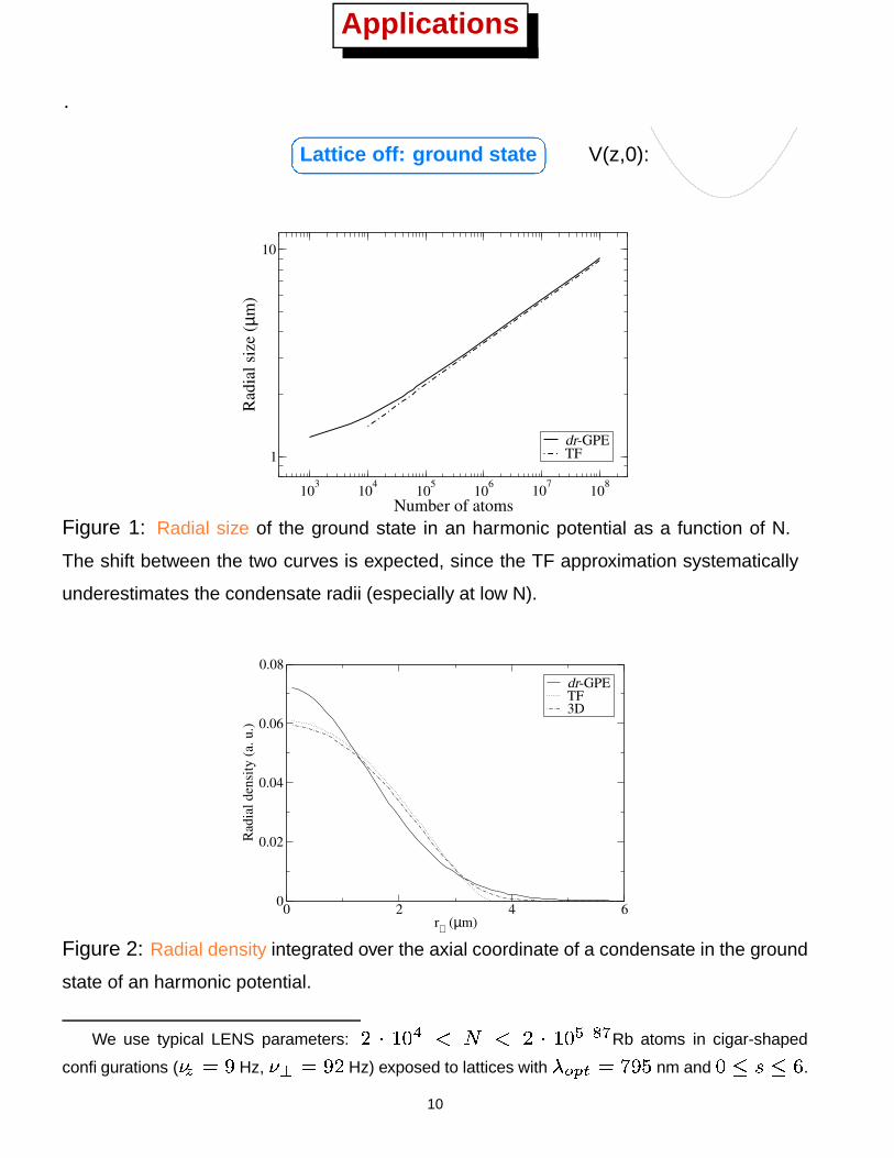
Applications

. �� ��Lattice off: ground state V(z,0):

0

10

20

30

40

50

60

70

-10 -5 0 5 10

103 104 105 106 107 108

Number of atoms

1

10Ra

dial

size

(µm

)

dr-GPETF

Figure 1: Radial size of the ground state in an harmonic potential as a function of N.

The shift between the two curves is expected, since the TF approximation systematically

underestimates the condensate radii (especially at low N).

0 2 4 6r⊥ (µm)

0

0.02

0.04

0.06

0.08

Radi

al d

ensit

y (a

. u.)

dr-GPETF3D

Figure 2: Radial density integrated over the axial coordinate of a condensate in the ground

state of an harmonic potential.

We use typical LENS parameters:

6 E � &�� � * �6 E � &������ Rb atoms in cigar-shaped

configurations ( � + Hz, 8 +

6Hz) exposed to lattices with

8 687�9 + ��� nm and

&�� �����.

10

��

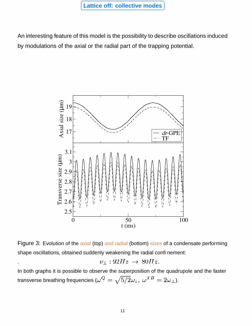
��Lattice off: collective modes

An interesting feature of this model is the possibility to describe oscillations induced

by modulations of the axial or the radial part of the trapping potential.

0 50 100t (ms)

2.52.62.72.82.9

33.1

Tran

sver

se si

ze (µ

m)

dr-GPETF

17

18

19

Axi

al si

ze (µ

m)

Figure 3: Evolution of the axial (top) and radial (bottom) sizes of a condensate performing

shape oscillations, obtained suddenly weakening the radial confinement:

. � 8 ��� 1�� & C � 3 � &��In both graphs it is possible to observe the superposition of the quadrupole and the faster

transverse breathing frequencies ( 6 " 2 /21 6�� > 6 � � " 1 6 8 ).

11

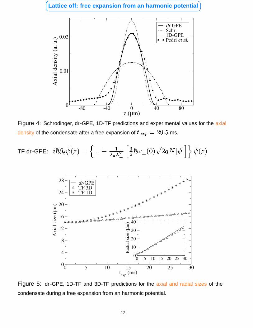
�� ��Lattice off: free expansion from an harmonic potential

-80 -40 0 40 80z (µm)

0

0.01

0.02

Axi

al d

ensit

y (a

. u.)

dr-GPESchr.1D-GPEPedri et al.

Figure 4: Schrodinger, dr -GPE, 1D-TF predictions and experimental values for the axial

density of the condensate after a free expansion of$�� � 7 " 1 � � ms.

TF dr -GPE:�0� � % 1 �32 �� � � � � � ���� � ! � ���� � � � � � � � � & � � 1 ��� 1 �32 �

0 5 10 15 20 25 30texp (ms)

0

4

8

12

16

20

24

28

Axi

al si

ze (µ

m)

dr-GPETF 3DTF 1D

0 5 10 15 20 25 300

10

20

30

40

Radi

al si

ze (µ

m)

Figure 5: dr -GPE, 1D-TF and 3D-TF predictions for the axial and radial sizes of the

condensate during a free expansion from an harmonic potential.

12

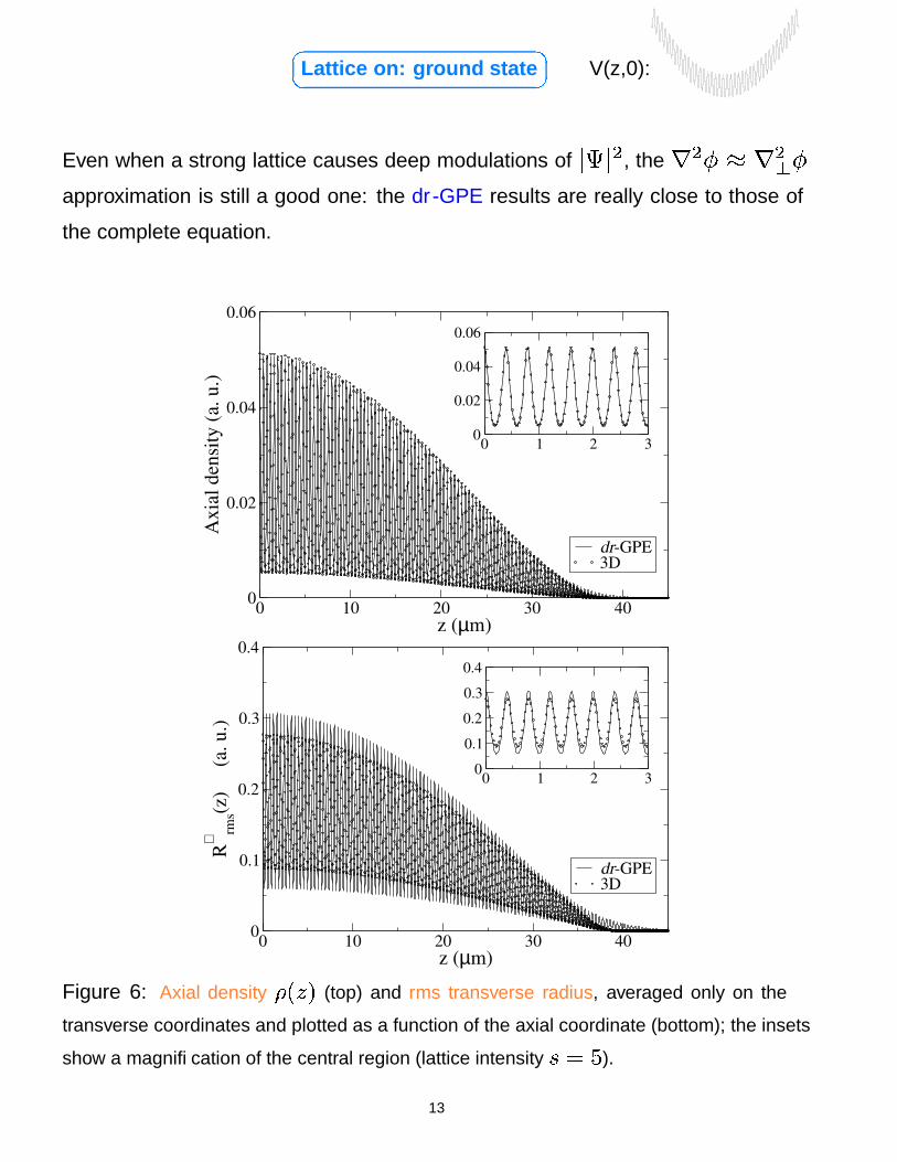
�� ��Lattice on: ground state V(z,0):0

10

20

30

40

50

60

70

-10 -5 0 5 10

Even when a strong lattice causes deep modulations of� � �

, the � � � D � � � �approximation is still a good one: the dr -GPE results are really close to those of

the complete equation.

0 10 20 30 40z (µm)

0

0.02

0.04

0.06

Axi

al d

ensit

y (a

. u.)

dr-GPE3D

0 1 2 30

0.02

0.04

0.06

0 10 20 30 40z (µm)

0

0.1

0.2

0.3

0.4

R⊥rm

s(z)

(a

. u.)

dr-GPE3D

0 1 2 300.10.20.30.4

Figure 6: Axial density � < & @ (top) and rms transverse radius, averaged only on the

transverse coordinates and plotted as a function of the axial coordinate (bottom); the insets

show a magnification of the central region (lattice intensity �" ).

13

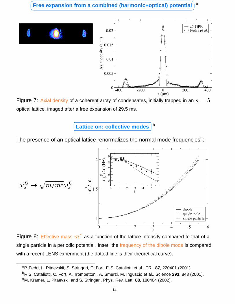
�� ��Free expansion from a combined (harmonic+optical) potential a

-400 -200 0 200 400z (µm)

0

0.005

0.01

0.015

0.02

Axi

al d

ensit

y (a

. u.)

dr-GPEPedri et al.

Figure 7: Axial density of a coherent array of condensates, initially trapped in an �"

optical lattice, imaged after a free expansion of 29.5 ms.

��

��Lattice on: collective modes b

The presence of an optical lattice renormalizes the normal mode frequenciesc:

� � ? F � ��� � ��

0 1 2 3 4 5 6s

1

1.5

2

m* / m

dipolequadrupolesingle particle

0 1 2 3 4 5s

5

6

7

8

9

ωzD

/2π

(Hz)

Figure 8: Effective mass 3 *as a function of the lattice intensity compared to that of a

single particle in a periodic potential. Inset: the frequency of the dipole mode is compared

with a recent LENS experiment (the dotted line is their theoretical curve).

aP. Pedri, L. Pitaevskii, S. Stringari, C. Fort, F. S. Cataliotti et al., PRL 87, 220401 (2001).bF. S. Cataliotti, C. Fort, A. Trombettoni, A. Smerzi, M. Inguscio et al., Science 293, 843 (2001).cM. Kramer, L. Pitaevskii and S. Stringari, Phys. Rev. Lett. 88, 180404 (2002).

14

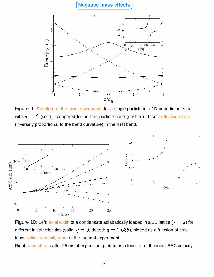
�� ��Negative mass effects

-1 -0.5 0 0.5 1q/qB

0

2

4

6

8

Ener

gy (a

.u.)

0 0.2 0.4 0.6 0.8 1q/qB

-5

0

5

m*/

m

Figure 9: Structure of the lowest two bands for a single particle in a 1D periodic potential

with �" 1 (solid), compared to the free particle case (dashed). Inset: effective mass

(inversely proportional to the band curvature) in the first band.

0 5 10 15 20 25t (ms)

20

25

30

Axi

al si

ze (µ

m)

0 5 10 15 20 25t (ms)

0

1

2

3

s

0 0.5 1 1.5q/qB

1

1.5

2

2.5

Asp

ect r

atio

Figure 10: Left: axial width of a condensate adiabatically loaded in a 1D lattice ( �" 1 ) for

different initial velocities (solid: �" 3 , dotted: �

" 3 ��� � ), plotted as a function of time.

Inset: lattice intensity ramp of the thought experiment.

Right: aspect ratio after 25 ms of expansion, plotted as a function of the initial BEC velocity.

15

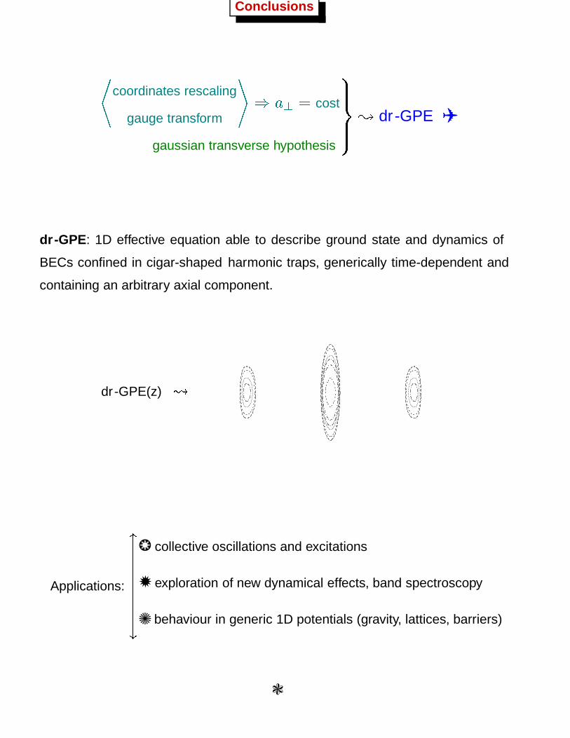
Conclusions

coordinates rescaling

gauge transform

* & � cost

gaussian transverse hypothesis

� ������ � dr -GPE ✈

dr -GPE: 1D effective equation able to describe ground state and dynamics of

BECs confined in cigar-shaped harmonic traps, generically time-dependent and

containing an arbitrary axial component.

dr -GPE(z)J

1e-05 2e-05 6e-05 0.0001 0.0002 0.0006

-400 -200 0 200 400

-100

-50

0

50

100

Applications:

������������

❂ collective oscillations and excitations

✹ exploration of new dynamical effects, band spectroscopy

✺ behaviour in generic 1D potentials (gravity, lattices, barriers)

❃

16