Embed Size (px)
Citation preview

Coordinated Jacobian Transpose Controland its Application to a Climbing Machine
by
Craig Daniel Sunada
Bachelor of Science in Mechanical EngineeringUniversity of Colorado, Boulder (1992)
Submitted to theDepartment of Mechanical Engineering
in partial fulfillment of the requirements for the degree of
Master of Science in Mechanical Engineering
at the
Massachusetts Institute of Technology
August 1994
© 1994 Massachusetts Institute of Technology
Signature of AuthorDepartment of Mechanical Engineering
August 21, 1994
Certified by // V, _--_!_/ Steven Dubowsky
Thesis Supervisor
Accepted by -Ain A. Sonin
Chairman, Departmental Graduate Committee
Raotw %
MASSACHUSETTS INSTITUTE
0 C1 2 : 1994

Coordinated Jacobian Transpose Controland its Application to a Climbing Machine
Submitted to theDepartment of Mechanical Engineering
in partial fulfillment of the requirements for the degree ofMaster of Science in Mechanical Engineering
by
Craig Daniel Sunada
AbstractThis thesis proposes a control algorithm based on Jacobian Transpose Control for
coordinated position and force control of autonomous multilimbed mobile roboticsystems performing both mobility and manipulation. The technique is called CoordinatedJacobian Transpose Control, or CJTC. CJTC has advantages over other techniques usedto control multilimbed mobile robots, including being computationally inexpensive andproviding a simple and unified interface with higher level planners. It can also controlfunctions other than positions and orientations of the system. A methodology called theExtended Mobility Analysis is presented to choose a set of control variables that does notoverconstrain the system. The effectiveness of CJTC is demonstrated in laboratoryexperiments on a climbing system.
Thesis Supervisor: Dr. Steven Dubowsky
Title : Professor of Mechanical Engineering

Acknowledgments
Betsy, my love, thank you for your love, your support, and your understanding. Inever dreamed that love could be so overwhelming before we met. Alex, even though
you are still too young to understand what I say, thank you for being such a wonderful
son. I am ever so grateful that you are much better behaved than I was at your age.Thank you also for reminding me just how small my work is compared to the miracles
that surround me every day.
To my parents, who provided the guidance and inspiration that led me to MIT, this
thesis is proof of your accomplishments as parents and teachers of me. I hope that I can
do as well for my son. To my brother Wade: our rivalry helped spur me to greater
heights than I would have achieved alone.
To the rest of my family: Glen, Aunt Dorothy, Aunt Grace, Granny, Aunt Tania, and
all the others, thank you for your support. The strong foundation of the love that myfamily shares allowed me to reach these levels.
Rick and Lucy, thank you for your support. Even though I have only known you fortwo years, you are already family in my heart. Hopey, even though you will never
comprehend anything, you still give me your unconditional love.
Bob and Fran, thank you for your hospitality. You have made me feel welcome in this
strange, hostile city. Sophie and Hannah, I hope that you also strive for educational
excellence, and that in some small way I helped inspire you.
Dr. Dubowsky, thank you for providing me with insight and guidance in much more
than just academics and research. Someday I will tell my students your stories (or stories
about you).
Tom, thank you for your friendship, as well as your technical help. I would like to
thank Dalila Argaez for her contribution to my work: she started it all! I would like to
thank my fellow students for their assistance during my research: Jeff Cole, NathanRutman, Richard Wang, Michelle Tescuiba, and Pengyun (Perry) Gu. I hope to see youall at my next barbeque! Joe Deck, thanks for imparting upon me some of your
perspective on life at MIT.
The support of this work by NASA (Langley Research Center, Automation Branch)under Grant NAG-1-801 is acknowledged.

Table of ContentsAbstract ........................................................................................................................... 2Acknowledgments .................................................................................................. 3Table of Contents .................................................................................................... 4List of Figures ......................................................................................................... 5Nomenclature: ........................................................................................................ 61: Introduction ......................................................................................................... 7
1.1: Purpose and Contributions .......................................... .......................... 71.2: M otivation ............................................................................................. 81.3: Background .................................................................................................. 10
1.3.1: Existing M ultilimbed M obile Robots .................................... . 101.3.2: Control algorithms ..................................... ........... 12
1.4: Assumptions................................................................................................. 162: Control Scheme Development .................................................................................... 19
2.1: Jacobian Transpose Control ......................................................................... 192.1.1: Derivation of Jacobian Transpose Control ................................... 21
2.2: Coordinated Jacobian Transpose Control .................................................... 222.2.1: Derivation of Coordinated Jacobian Transpose Control ............ 23
3: Control Vector Selection....................................................................................... 263.1: Control Variables ............................................................ ....................... 263.2: Control Vector Selection ..................................................................... ... 27
3.2.1: Gruebler's M obility Analysis ......................................... .... .283.2.2: Extended M obility Analysis ......................................................... 31
4: Application of CJTC to a laboratory climbing robot ....................................... 394.1: System description ..................................................................... 39
4.1.1: Climbing M achine ...................... ............ ........... 404.1.2: Power Amplifiers ......................................................................... 434.1.3: Control Computers ................................................ 43
4.2: Climbing Gait............................................................................................... 444.3: Control Vector Selection........................... ...................................... 454.4: Control equations .................................................................................. 514.5: Control gain selection .............................................................................. 53
4.5.1: Dynamic M odel ....................................... 534.6: Experimental performance ................................................................... ........ 57
4.6.1: Data from climbing stage one ....................................................... 574.6.2: Data from a full climbing cycle ................................................... 61
5: Summary and Conclusions ................................................................ 676: References .................................................................................................................. 68Appendix A: LIBRA Jacobian Equations ....................................................................... 73Appendix B: Power Amplifiers..................................................................................... 77Appendix C: Gain Selection ......................................................... ............................ 84Appendices References .................................................................................................. 98

List of Figures
Fig. 1: A Schematic of the LIBRA climbing system ..................................... 8Fig. 2: A multilimbed mobile robot ........................................................... 9Fig. 3: A representative multilimbed mobile robot ..................................... 18Fig. 4: Block Diagram of Jacobian Transpose Control .................................... 20Fig. 5: 2-link manipulator controlled through JTC .................................... . 20Fig. 6: Multilimbed Mobile Robotic system controlled through CJTC.......... 23Fig. 7: Block Diagram of CJTC ......................................... .............. 24Fig. 8: Common Planar Constraints ........................................ ........... 30Fig. 9: Stage One of the Extended Mobility Analysis ..................................... 33Fig. 10: Stage two of the Extended Mobility Analysis ................................... 35Fig. 11: Over actuated system ................................................................... 36Fig. 12: Over actuated system with environmental and internal constraintsrelaxed ................................................................................................................. 36Fig. 13: The LIBRA climbing system.................................. ............ 39Fig. 14: LIBRA system block diagram ...................... ......... 40Fig. 15: A Schematic of the LIBRA ....................................... ........... 41Fig. 16: Climbing Gait used by the LIBRA ............................................... 44Fig. 17: LIBRA under full environmental constraints ..................................... 45Fig. 18: Constraining x of the Center Body ......................................... ...... 46Fig. 19: Constraining x,y of the Center Body .................................................. 46Fig. 20: Constraining x,y,0 of the Center Body ............................................... 47Fig. 21: Constraining x,y of Foot 3 ........................................ ........... 47Fig. 22: Relaxing the x environmental constraint ...................................... 48Fig. 23: LIBRA with control vector 1 ....................................... .......... 49Fig. 24: LIBRA with control vector 2....................... .......... 50Fig. 25: LIBRA with control vector 3 .......................................................... 51Fig. 26: Model of the LIBRA top kinematic chain ..................................... 54Fig. 27: Dominant poles of the LIBRA for ybody from -0.20m -> 0.14 m........ 56Fig. 28: Desired motion for the climbing robot ....................................... 58Fig. 29: xb, Yb position for a pushup maneuver ....................................... 59Fig. 30: Ob for a pushup maneuver.................. .... ................ 59Fig. 31: x2 Force for a pushup maneuver.............................. ........... 60Fig. 32: x3 location for a pushup maneuver ......................................... ...... 60Fig. 33: Desired Cartesian movements for one gait cycle ............................... 61Fig. 34: Actual Cartesian movements for one gait cycle ................................. 62Fig. 35: Body movements for one gait cycle ....................................... ..... 63Fig. 36: Body orientations for one gait cycle ....................................... ..... 63Fig. 37: x positions for all the feet for one gait cycle .................................. .64Fig. 38: y positions for all the feet for one gait cycle ..................................... 64Fig. 39: Foot 1 position vs. time for one gait cycle .................................... .65Fig. 40: Foot 2 position vs. time for one gait cycle .................................... .65Fig. 41: Foot 3 position vs. time for one gait cycle .................................... .66Fig. B 1: Power amplifier schematic ................................................................ 78Fig. B2: Power Amplifier Card Layout .................................... ......... 79Fig. Cl: Model of the LIBRA .......................................... ............... 84Fig. C2: Poles of the LIBRA for ybody from -0.20m -> 0. 14m ...................... 93Fig. C3: Dominant poles of the LIBRA for ybody from -0.20m -> 0.14 m ....... 94Fig. C4: Bode plot for the xbody position variable................................... 95Fig. C5: Bode plot for the ybody position variable................................. 96Fig. C6: Bode plot for the qbody position variable................................... 97
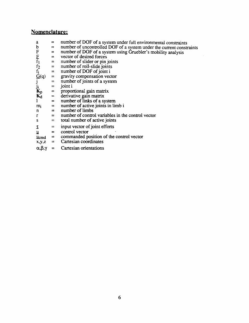
Nomenclature:
a = number of DOF of a system under full environmental constraintsb = number of uncontrolled DOF of a system under the current constraintsF = number of DOF of a system using Gruebler's mobility analysisF = vector of desired forcesfl = number of slider or pin jointsf2 = number of roll-slide jointsfi = number of DOF of joint iG(q) = gravity compensation vectorj = number of joints of a systemJi = joint i
p = proportional gain matrix= derivative gain matrix
1 = number of links of a systemmi = number of active joints in limb in = number of limbsr = number of control variables in the control vectors = total number of active jointst = input vector of joint effortsu = control vectorMcmd = commanded position of the control vectorx,y,z = Cartesian coordinatesa,4,y = Cartesian orientations

1: Introduction
1.1: Purpose and Contributions
The purpose of this thesis is to develop a control technique that can control both
mobility and manipulation of a multilimbed mobile robot while being computationally
feasible for small on-board computers. Mobility refers to the locomotion of the robot,
whether through walking, climbing, sliding, or other forms of limbed locomotion, and
manipulation refers to the interaction forces exerted on a task and the manipulation of an
object in the environment. Here, an approach called Coordinated Jacobian Transpose
Control, or CJTC, is proposed for the control of multilimbed, multi-degree of freedom
mobile robotic systems. An extension of classical Jacobian Transpose Control, CJTC
uses the simplest form of impedance control and an extended Jacobian matrix to control
the entire system's forces and motions in a consistent and coordinated manner while being
computationally feasible for small on-board computers. The effectiveness of CJTC is
demonstrated in laboratory experiments on a three-limbed climbing system called the
Limbed Intelligent Basic Robotic Ascender, or LIBRA, shown schematically in Figure 1.
This system was designed and built by Dalila Argaez, and she first proposes the concept
of CJTC 1. This thesis develops her concept into a working control scheme and
demonstrates its effectiveness. This first chapter presents the motivation for studying
multilimbed mobile robots, and the need for new control algorithms to control
simultaneously their movements and interaction forces with the environment.

Fig. 1: A Schematic of the LIBRA climbing system
1.2: Motivation
The area of multilimbed mobile robots is an expanding field, with many important
applications. It is becoming increasingly clear that multilimbed mobile robots are going
to be important for performing tasks in areas that are either inaccessible to humans or
undesirable or unsafe for humans to work. Such applications include toxic waste
handling and work at nuclear sites 2, 3, 4, 5, 6, 7. Multilimbed mobile robots are virtually
the only feasible solution for planetary exploration 8, 9, 10. These tasks take place in
partially structured environments, where the general characteristics and layout of the
terrain and tasks are known, but the specific details are not. Most of these tasks require

the robot to interact with the environment -- taking measurements and manipulating
objects. Manipulation tasks may require carefully controlled forces to be applied. Often,
the manipulation tasks will have to be performed while also moving the robot. For
instance, a mechanical monkey might scurry into a toxic waste area and carefully take
some measurements. Another part of its task might be to then shut off a valve, and then
pick up a waste drum and carry it out. An example of a multilimbed robotics system is
shown schematically in Figure 2, with limbs that are capable of both mobility and
manipulation. As discussed in the next section, no multilimbed mobile robotic system in
existence today is capable of performing tasks requiring both mobility and manipulation
simultaneously, and that new control algorithms need to be developed to perform such
tasks.
aition
Fig. 2: A multilimbed mobile robot
TT · ~~+~1~~ rr r I·~~·L·~H
------
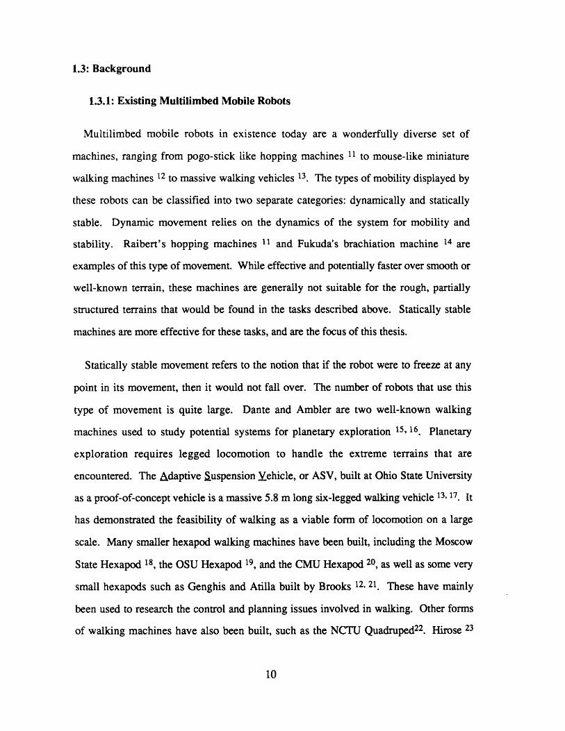
1.3: Background
1.3.1: Existing Multilimbed Mobile Robots
Multilimbed mobile robots in existence today are a wonderfully diverse set of
machines, ranging from pogo-stick like hopping machines " to mouse-like miniature
walking machines 12 to massive walking vehicles 13. The types of mobility displayed by
these robots can be classified into two separate categories: dynamically and statically
stable. Dynamic movement relies on the dynamics of the system for mobility and
stability. Raibert's hopping machines 11 and Fukuda's brachiation machine 14 are
examples of this type of movement. While effective and potentially faster over smooth or
well-known terrain, these machines are generally not suitable for the rough, partially
structured terrains that would be found in the tasks described above. Statically stable
machines are more effective for these tasks, and are the focus of this thesis.
Statically stable movement refers to the notion that if the robot were to freeze at any
point in its movement, then it would not fall over. The number of robots that use this
type of movement is quite large. Dante and Ambler are two well-known walking
machines used to study potential systems for planetary exploration 15, 16. Planetary
exploration requires legged locomotion to handle the extreme terrains that are
encountered. The Adaptive Suspension Yehicle, or ASV, built at Ohio State University
as a proof-of-concept vehicle is a massive 5.8 m long six-legged walking vehicle 13, 17. It
has demonstrated the feasibility of walking as a viable form of locomotion on a large
scale. Many smaller hexapod walking machines have been built, including the Moscow
State Hexapod 18, the OSU Hexapod 19, and the CMU Hexapod 20, as well as some very
small hexapods such as Genghis and Atilla built by Brooks 12, 21. These have mainly
been used to research the control and planning issues involved in walking. Other forms
of walking machines have also been built, such as the NCTU Quadruped22. Hirose 23

built Titan III, a quadruped that is capable of both statically stable and dynamic walking.
Multilimbed mobile robotic systems used for climbing include the Portsmouth
Polytechnic Robug II, which uses vacuum grippers to climb walls 24. Neubauer 25 built a
6 legged climbing machine that uses friction to climb between two walls. Gradetsky et.
al. 26 discuss a climbing robot using vacuum grippers for actuation. Hirose 27 has also
built a climbing machine with vacuum grippers, capable of both statically stable and
dynamic walking. While these walking and climbing machines have demonstrated
substantial capabilities, none of these systems are capable of manipulation.
While mobility is certainly the first step in field robotic systems, manipulation must
also be addressed. Even the field robots such as Dante aren't capable of manipulation,
but rather are used simply to position sensors. The ability to collect ground samples,
move obstacles, and probe the environment would all enhance the utility of Dante as a
terrestrial exploration robot. One robot that is capable of both mobility and manipulation
is the Savannah River Nuclear Mobile Robot -- a hexapod robot with a manipulator
mounted on top 28. However, during manipulation tasks the base is usually stationary and
it is not capable of controlling both mobility and manipulation simultaneously. Despite
this significant drawback, it has been found to be useful enough to warrant a second
generation of the design. There are also a number of mobile robots that use tracks or
wheels for mobility rather than limbs have been built and used that are capable of
manipulation and have proven to be quite useful. HAZBOT, for instance, is used for
hazardous materials handling 7, and the Foster Miller Ferret has proven to be very
effective in explosives handling 29.
While the current designs of multilimbed mobile robots largely ignore manipulation or
treat manipulation separately from mobility, given the usefulness of other systems
capable of both mobility and manipulation, new multilimbed mobile robots are sure to be

developed that will be capable of simultaneous mobility and manipulation. In order to
control these future systems, new control schemes will need to be developed.
1.3.2: Control algorithms
Control algorithms that would allow the control of manipulation forces and motions
while simultaneously controlling the trajectory of the rest of the system have yet to be
developed for multilimbed mobile robots. The Savanahh River Nuclear Robot, a current
experimental multilimbed mobile robotic system capable of both mobility and
manipulation, treats mobility and manipulation separately -- performing only one or the
other at a time. It also does not control the forces exerted on the environment 28. In order
to increase the utility of robots, new control approaches must be developed to control
simultaneously the motions of such articulated multilimbed mobile robotic systems and
the forces that they exert on their environment or tasks. One way to develop new
approaches is to attempt to extend the current methods used for mobility to also include
manipulation, or to attempt to extend current methods used for manipulation to also
include mobility.
A significant amount of work has been done in the area of the control of walking
machines. A common form of control currently used is simple joint space position
control. However, this form of control cannot directly control the forces being applied to
the environment, and therefore isn't applicable for the control of forces during
manipulation. Joint space position control also produces rough, jerky motion of the body
of the robot in Cartesian space, and is difficult to adapt for rough terrain and changes in
the environment 30. A form of force control is therefore required.
A common form of control used that controls the forces being applied to the
environment is called coordinated walking. Coordinated walking is an inverse plant
controller, and like other forms of inverse plant controllers, coordinated walking is

computationally expensive, requires a detailed model of the system, and is sensitive to
modeling errors 31. One form of coordinated walking treats the legs as force servos and
resolves the desired motions and a force distribution algorithm into forces to be applied
by the legs 32, 33. This type of controller has demonstrated problems associated with
practical difficulties in getting the legs to act like high-performance force servos 30. Also,
the system performance is low because the bandwidth of the overall trajectory controller
must be substantially less than the bandwidth of the legs' controllers 31. Designing this
type of coordinated walking is difficult because of the sensitivity to modeling errors.
Without incorporating the often difficult to model actuator dynamics in the controller or
analysis, the control gains must be chosen by trial and error 31. Another form of
coordinated walking includes a simple model of the actuator dynamics in its model of the
system, and directly reflects the desired trajectory and limb forces to the limb actuators
31. While this controller offers several advantages, such as the ability to decouple the
system and linearize the control, it is also very computationally expensive. The ASV,
which uses this control scheme, has 16 dedicated processors for the control alone 13
Coordinated walking does not address the issue of manipulation. Although it might be
possible to extend coordinated walking to include manipulation, the computational
burden would be large. While this is acceptable on large systems such as the ASV that
can carry powerful computers, for small self-contained systems with small capability
processors, this would not be feasible. Also, the sensitivity to modeling errors would
pose a problem when manipulating an object in a partially known field environment
where a detailed model of the object is not available. Given the limitations of that this
controller would have, another approach for controlling mobility and manipulation is
desired.
Looking for another way to develop a control algorithm to control both mobility and
manipulation, control techniques that are currently used for manipulation are examined to
see if they could be extended to also control mobility. There are two primary forms of

force control used to control fixed base serial manipulators -- hybrid control and
impedance control. Khatib shows how generalized joint torques are reflected at the end-
effector for redundant manipulators, an important understanding for either form of force
control of redundant manipulators 34. Raibert and Craig propose a hybrid control scheme
to control manipulator motions to satisfy position and force constraints simultaneously,
and have demonstrated this approach through controlling the end-effector of a two link
fixed-based manipulator 35. Hybrid control can also be extended to systems other than
simple serial manipulators. For instance, Yoshikawa and Zheng extend hybrid
position/force control to multiple robot manipulators working in well-known
environments 36. However, hybrid control techniques require detailed knowledge of the
environment for effective force control, including a good estimate of the environmental
stiffness 37. Since such an estimate probably would not be available in a partially known
environment, hybrid control is not suitable for this research.
Impedance control is the other primary form of force control. Hogan introduced
impedance control, which controls a relationship between force and displacement, as a
unified method for controlling the force and the position of a manipulator's end-effector
38, 39. Hogan also asserts that it is possible to superimpose impedances, which is
necessary if multiple degrees of freedom are to be controlled. Schneider and Cannon use
Hogan's impedance control approach to arrive at an object impedance controller for
cooperative manipulation, which gives a straightforward interface for supervisory control
by directly controlling the object being manipulated 40, 41. Impedance control has
demonstrated good stability in contact transitions -- a quality than many other force
control schemes lack 42. It also does not require precise knowledge of the environment,
in contrast to hybrid control. Some simple forms of impedance control don't even require
a dynamic model of the system. Given these characteristics, impedance control is
promising as a possible controller for both mobility and manipulation.

Current control techniques that deal with mobility and manipulation are investigated
for possible methods to extend impedance control to control simultaneous mobility and
manipulation. A number of control algorithms have been developed for motion control
of manipulators mounted on simple vehicles, such as on spacecraft and trucks 43, 44
Hootsmans and Dubowsky use an extended Jacobian matrix to compensate for base
dynamics while using Jacobian Transpose Control to control a manipulator mounted on a
mobile base 45. However, these algorithms only look at manipulation while
compensating for base movements and do not actively control the base. Seraji, on the
other hand, proposes an extended Jacobian matrix to actively control the motions of a
system composed of a manipulator mounted on a track or otherwise mobile base through
inverse Jacobian control 46, 47. His control algorithm was demonstrated experimentally
on a 7 DOF robot arm mounted on a motorized track 48. The use of an extended Jacobian
matrix might allow impedance control to control both mobility and manipulation.
While there currently is no control algorithm reported in the literature that controls
both the mobility and manipulation of a multilimbed mobile robot, several promising
avenues exist. As discussed before, coordinated walking could be extendible to control
manipulation, but would probably be too computationally expensive for this problem.
Impedance control, currently used for manipulation with serial arms, is promising for
both the ability to control the position of the end-effector while it is free and the forces it
exerts while constrained, and for stability during contact transition. The use of an
extended Jacobian matrix, similar to Seraji 46, 47 or Hootsmans 45 might enable
impedance control to control multiple points on a robot in order to control both
manipulation and mobility, and this is the approach pursued in this research.

1.4: Assumptions
The need for developing a new control algorithm that controls both mobility and
manipulation has been discussed, but the exact problem domain remains to be defined.
The range of systems and tasks that could be covered by the terms 'multilimbed mobile
robot' is too large to be covered by any single control scheme, and specific assumptions
need to be made to limit that range. Assumptions are made about the nature and
requirements of the environments and tasks, the computational capability and the
kinematics of the class of robots to be controlled.
It is assumed that the robot is operating in a partially known environment. This
implies that the general nature of the environment is known, and perhaps even the general
layout of the environment and task, but the precision to which these things are known
beforehand is not great, perhaps to within 5% or 10% of the limb span of the robot. The
order of magnitude of the environmental stiffness might be known, and an approximate
mass of an object to be manipulated, but detailed models will not be available. This
assumption is representative of robots working in field environments, and prevents the
use of control schemes that require good knowledge of the environment, such as hybrid
control. It also prevents the use of control schemes that require a detailed dynamic model
of the task and environment.
It is assumed that the task will require the forces being applied to the task to be
controlled, but not to great precision. This assumption is made to allow a control scheme
without force feedback. It is also assumed that for all tasks, all degrees of freedom of the
system under the full kinematic constraints imposed by the environment must be
controlled. This is generally required for acceptable system performance 49.
It is assumed that the computational capability will be from a single processor of
medium capability -- approximately the capability of an Intel 80386 processor or a

Motorola 68020. This represents an accessible amount of processing capability for
almost any size except for very small systems.
These assumptions are not suitable for every multilimbed mobile robotic system, and
limit the applicability of the control scheme developed in this thesis. Also, many of these
assumptions are qualitative, and are meant as guidelines. As technology changes and
additional sensors, actuators, and computational capability become readily available,
many of the assumptions made may be relaxed. For instance, if much more processing
capability is readily available, then it might be desirable to develop other control
techniques that take advantage of that fact and subsequently give better performance.
The following is a description of the kinematics of the class of robots to be treated in
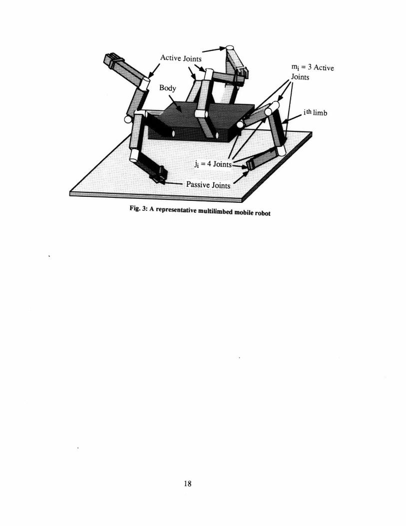
this thesis. Figure 3 shows an n-limbed mobile robotic system representative of the class
of robots dealt with herein. The system contains one main body with the n limbs attached
and a base, which represents the ground. Some of the limbs position the main body with
respect to ground for mobility purposes, while the remaining limbs may perform
manipulation tasks or be free. It is assumed that the ith limb is a ji joint serial chain where
mi of the joints are active and (ji-mi) joints are passive. Among the (ji-mi) passive joints,
some are passive due to the physical contact of the limb with the ground or a manipulated
object; the others are mechanical non-actuated joints. The total number of active joints
for the system is given by:
s= 1mi. (1)
The kinematic variables qi of the s active joints form a set that is referred to as the joint
vector g. The effort variables of the system's actuators, a torque for a revolute joint or a
force for a prismatic joint, are the inputs to the system; they form the s by 1 input vector
:. It is assumed that the actuators are backdrivable.
Active Joints
Fig. 3: A representative multilimbed mobile robot
Active
limb

2: Control Scheme Development
Looking at existing control techniques and given the assumptions made, a form of
impedance control is chosen to be extended to control both mobility and manipulation for
the following reasons. Given the need to actively control forces, either impedance
control or hybrid control could be used. Given the assumption of partially known
environments, hybrid control would have been difficult to implement. Impedance control
does not require exact knowledge of the environment. Given the restriction on
computational capability, the simplest form of impedance control, Jacobian Transpose
Control 37??? is used. This control does not require the use of force sensors for feedback,
which might be advantageous for some systems. Controlling forces without force
feedback is only possible with the use of backdrivable actuators, which is assumed in the
previous section.
2.1: Jacobian Transpose Control
Since Coordinated Jacobian Transpose Control is based on Jacobian Transpose
Control, this section first gives the derivation for classical Jacobian Transpose Control
(JTC). A complete analysis of Jacobian Transpose Control, including a Lyapunov
stability analysis, can be found in 37. Conceptually, Jacobian Transpose Control is
proportional-derivative control of the position of the end-effector (x) of a serial
manipulator in Cartesian space. JTC controls the dynamic relationship between force and
position, or the mechanical impedance of the end-effector. The end-effector is pulled
towards the commanded end-effector position by a set of virtual springs and dampers.
After calculating the vector of desired forces (E) from these virtual springs and dampers,
JTC directly transforms them into desired efforts at the actuators (:) through the
transpose of the Jacobian matrix J. A block diagram of the controller is shown in Figure

4. Figure 5 shows this concept applied to a simple two link serial manipulator, where the
end-effector Cartesian x and y positions are controlled.
Acmd
kmd
x
Fig. 4: Block Diagram of Jacobian Transpose Control
Uxcmd
:tor
Fig. 5: 2-link manipulator controlled through JTC
As with other impedance control approaches, when the end-effector is constrained in a
direction, a force is applied in that direction, and when the end-effector is unconstrained
in a direction, a motion results. A compliant constraint results in both a force and
displacement. Impedance control eliminates the need for switching between control
structures to control both the position when unconstrained and force when constrained.
This allows simple, intuitive control of the system. Jacobian Transpose Control is also
robust to parametric uncertainty both in the manipulator itself and in the environment,
and does not require a mass model of the manipulator. Although both position and force
q

control with Jacobian Transpose Control is not as high performance as some other control
schemes, it is quite acceptable and demonstrates good contact stability.
2.1.1: Derivation of Jacobian Transpose Control
The vector of Cartesian coordinates x of the end-effector is defined as:
x
yz
x = 1 (2)
Y
or a subset thereof, depending on the degrees of freedom the manipulator has.
The desired force vector F is defined to be:
F = K, -[xd - x] + Kd " ['.d - ] (3)
The gain matrices Kp and Kd determine the response of the system, and are chosen to
satisfy the controller design requirements. The gain matrices are generally chosen to be
diagonal, but can be non-diagonal if coupling between end-effector Cartesian coordinates
is desired.
The Jacobian is defined as the transformation between joint space velocities and
Cartesian velocities:
ax axaq, a q
_07 .. aq,-
(4)
The end-effector velocities are given by:
8u = J(q) - q (5)
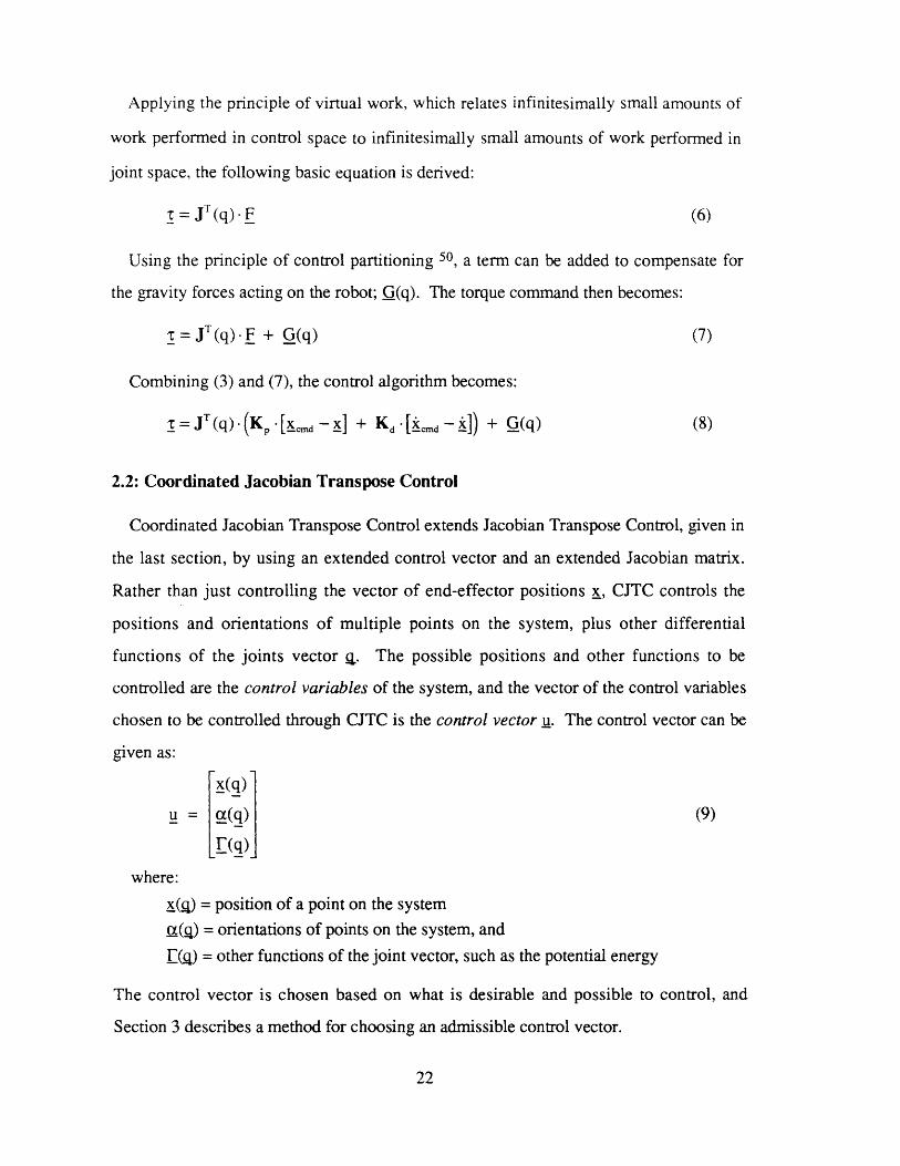
Applying the principle of virtual work, which relates infinitesimally small amounts of
work performed in control space to infinitesimally small amounts of work performed in
joint space, the following basic equation is derived:
t = (q). F (6)
Using the principle of control partitioning 50, a term can be added to compensate for
the gravity forces acting on the robot; G(q). The torque command then becomes:
S= JT (q) F + G(q) (7)
Combining (3) and (7), the control algorithm becomes:
= jT(q) (K, -[x - X] + Kd.[~md -k])+ G(q) (8)
2.2: Coordinated Jacobian Transpose Control
Coordinated Jacobian Transpose Control extends Jacobian Transpose Control, given in
the last section, by using an extended control vector and an extended Jacobian matrix.
Rather than just controlling the vector of end-effector positions x, CJTC controls the
positions and orientations of multiple points on the system, plus other differential
functions of the joints vector q. The possible positions and other functions to be
controlled are the control variables of the system, and the vector of the control variables
chosen to be controlled through CJTC is the control vector u. The control vector can be
given as:
[(q)
u= oX(q) (9)
where:
x(g) = position of a point on the system
Q(_) = orientations of points on the system, and
Iq() = other functions of the joint vector, such as the potential energy
The control vector is chosen based on what is desirable and possible to control, and
Section 3 describes a method for choosing an admissible control vector.

Conceptually, Coordinated Jacobian Transpose Control is proportional-derivative
control in control space. Each element of the control vector is forced to move towards its
corresponding element of a desired or commanded control vector (Icmd) by a set of
virtual springs and dampers in the classical Jacobian Transpose Control approach. Figure
6 shows a multilimbed mobile robot under CJTC with the virtual spring-dampers applied
to the control vector.
) cm
Fig. 6: Multilimbed Mobile Robotic system controlled through CJTC.
2.2.1: Derivation of Coordinated Jacobian Transpose Control
The derivation for CJTC closely follows that of Jacobian Transpose Control, and some
of the same equations will be referenced. A block diagram of the control scheme is given
in Figure 7. The additional block for sensors is required if one or more of the control
variables are functions of other variables in addition to the joint vector q. In this case,
sensors are required that can measure these other variables.

-mcmd
Aýcmd
Sensors
Fig. 7: Block Diagram of CJTC
The (rx1) desired force vector E is defined to be:
F= K, -[umd - u] + Kd -[ •md - u ] (10)
where r is the number of control variables in the control vector
Again, the gain matrices Kp and Kd are generally chosen to be diagonal, and are chosen
to satisfy the controller design requirements. Each element of the force vector (F) results
in an acceleration of the system if the corresponding element of the control vector (u) is
unconstrained or in a force applied to the environment if the corresponding element of the
control vector is constrained.
The extended Jacobian is defined as the transformation between joint space velocities
and control space velocities:
au 1 au1aqq ....... aq,
aur aur
aqý" aq.Bu._. Bu...z•qu 3u
ax, ax,
d-II aq.d ....... qs
The Jacobian is r by s, where r 5 s is the number of control variables and s is the total
number of active joints. The Jacobian does not need to be square, and some redundancies
(11)J(q) =

can be left uncontrolled if they are not important for the system performance. Combining
(7), (10) and (11), the control algorithm becomes:
T = J (q) -(K -[ucmd - u] + K, -[md - u_) + G(q) (12)
Coordinated Jacobian Transpose Control for multilimbed systems has the same
advantages that Jacobian Transpose Control offers for serial manipulators. Namely, only
the forward kinematics and their derivatives are required, implying a relatively small
number of computations. No inertial model of the robot is required. Also, the Jacobian
matrix can be rectangular, which is of great importance for redundant systems. CJTC is
also robust to parametric uncertainties in both the robot itself and in the environment.
Finally, this control scheme provides an intuitively simple interface for controlling end-
point positions and forces of a multilimbed system. By moving the commanded
endpoints through space or into an object, the limb moves or pushes accordingly. By
controlling all the control variables in this fashion, straightforward integration is achieved
with higher level planning algorithms.
However, CJTC does not compensate for the changing dynamics of the system, and as
a result the performance is configuration dependent. The extent of the configuration
dependence is a function of the mass distribution of the robot. When selecting the gain
matrices, the controller must be designed for the worst-case configuration 51. If the
dynamic response varies dramatically, then performance will be sacrificed significantly
over the majority of the workspace. If this is the case, gain scheduling or other forms of
adaptation might be required. Also, no attempt is made to decouple the system, and
significant coupling between control variables can occur. This can be compensated for
by using a non-diagonal gain matrix, but the degree of coupling is configuration
dependent and adaptive control or gains scheduling might be required. Despite these
characteristics, it will be demonstrated that the control system performance is quite
acceptable for the LIBRA climbing robot.

3: Control Vector Selection
The control algorithm derived in the previous section operates on the control vector u,.
and the method for choosing the control vector is presented in this section. The control
vector is chosen by the designer, based on the task and the environmental constraints.
CJTC allows considerable freedom in choosing the control vector, and this allows the
designer to directly control the control variables of interest. The points made in this
section are based on general control theory, but are tailored specifically for the CJTC,
with all the assumptions and restrictions given in Section 1.4.
3.1: Control Variables
Any differentiable mathematical function of g with non-zero first partial derivatives
with respect to q that describes a physical property of the system is defined to be a
control variable. For instance, the Cartesian coordinates x, y and z of a point on the
system are functions of q and are three possible control variables. The Cartesian
orientations a, 13, and y of a point on the system are also possible control variables. The
most basic control variables are the joint displacements. More abstract control variables
might include the system's potential energy or a static stability function to prevent the
robot from tipping over. For any given system, there are an infinite number of possible
control variables. Of these possible control variables, an admissible set must be chosen
to control. A methodology called the Extended Mobility Analysis for choosing an
admissible set of control variables is described below. The set of chosen control
variables is called the control vector u. The space of control vectors corresponding to all
possible configurations of the system is called the control space.
In order to reflect the control errors to the actuators through the Jacobian matrix, the
control variables must be written in terms of the joint vector _q. In order to do so, the
control variables will generally be written using the assumed environmental constraints
both implicitly and explicitly. Since the control variables are functions of the joint vector
g, joint position sensors are needed for joint vector feedback. If the control variables are
also functions of other variables, then sensors that can measure those variables are also
required. Additional sensors might be required to obtain the initial position, to check the
position during the movement and correct for errors caused by unexpected slipping, but
are not required by the control scheme.
3.2: Control Vector Selection
Choosing the control vector n is not trivial. While the joint vector g is imposed on the
system by the mechanical design, the control vector u is chosen by the designer. The
designer must choose an admissible set from the infinite number of possible control
variables, based on the tasks a specific system must perform, the environmental
constraints placed on the system, and desirable performance characteristics. Since the
range of possible control variables is so diverse, it is often possible to directly control the
points or functions of interest. For instance, if visual feedback from a camera mounted
on the robot is important, then good choices for control variables would be the positions
and orientations of the camera. If the location of the center of mass of the body is more
important, then it is possible to directly control that as well. As stated in the problem
definition, all the degrees of freedom of a system under the full kinematic constraints
imposed by the environment must be controlled. The environmental interaction forces or
other control variables do not have to be controlled, but it often is desirable to do so.

It is important to note that the control vector will change during a robot's mission,
based on the changing constraints and desired tasks that the robot will perform. For
mobility, it is necessary to lift and maneuver a foot at certain times in the gait, and use
that foot to support the body at others. So, for the different tasks and constraints,
different control vectors must be chosen. Given the constraints that the system will be
subject to, an Extended Mobility Analysis can be performed to determine admissible
control vectors.
For the s active joints of the system, s control variables are possible to control. At the
lowest level, the s individual active joint positions can be controlled. However, it is not
necessary to control all s possible control variables. Sometimes, after choosing a number
of important control variables to control, the only control variables admissible to
complete the control vector are unimportant for the system. In such cases, it might be
wise not to waste the computing resources needed to control these unimportant control
variables. When deciding whether to control these unimportant control variables, the
designer should consider just how important the control variables are to the system, and
how much computing capability is available.
3.2.1: Gruebler's Mobility Analysis
A brief summary of Gruebler's Mobility analysis is given here for review, since it is
heavily relied upon in the Extended Mobility Analysis. In this thesis, the term 'mobility
analysis' refers to Gruebler's Mobility Analysis. This review is not complete, and a more
complete description of Gruebler's Mobility Analysis is given in 52.
An unconstrained rigid body in spatial motion has six degrees of freedom, the x, y, z
translations and the a, J3 and y rotations. A mechanism constructed of I rigid links will

have 6-1 degrees of freedom before they are connected to form a system of links. The
connections constrain the system and result in losses of degrees of freedom of the system.
Different forms of connectors constrain various numbers of degrees of freedom. A pin
joint, one type of lower-pair connector, constrains the three translational degrees of
freedom and permits only rotation in one direction. For instance, a link connected to
ground through a pin joint has but one degree of freedom, and therefore lost five of the
six degrees of freedom it had when unconstrained. A slider joint, another type of lower-
pair connector, also constrains five degrees of freedom, as it only allows movement in
one translational direction. Another type of constraint is referred to as the roll-slide
contact. Two bodies are in contact, but can translate across each others' surfaces and also
rotate with respect to each other. Only one degree of freedom -- translation in the normal
direction to the surfaces -- is constrained.
Gruebler's equation is now given as:
F = 6.(1-j-1) + Jfi (13)
where:F = the number of degrees of freedom of the system1 = the number of links, including the groundj = the number of joints, including ground contacts
fi = the number of degrees of freedom allowed by joint i
In planar motion, there are only three degrees of freedom -- the x and y translations and
the single rotation 0. Gruebler's equation in planar motion is given as:
F = 3.(1-1) - 2.fl - f2 (14)
where:
fl = the number of slider or pin joints
f2 = the number of roll-slide contacts

Figure 8, adapted from Sandor and Erdman 53, gives some common planar kinematic
joints and their appropriate degrees of freedom.
Diagram Characteristic Variables
Pin (revolute)
Slider (prismatic)
Rolling Contact
Roll-Slide Contact
Spring
1=2f= 1
f2=0fi = 1
1
2ZZ 777117777
12
2
1
1=2fl= 1
f2=0fi = 1
degree of freedom
degree of freedom
1=2fl=1
f2=0fi = 1 degree of freedom
1=2fl =0f2= 1fi = 2 degrees of freedom
1=2fl=0f2=0fi = 3 degrees of freedom
Fig. 8: Common Planar Constraints
Joint
2
2

3.2.2: Extended Mobility Analysis
The Extended Mobility Analysis is based on Gruebler's mobility analysis. It addresses
which sets of control variables can be controlled for a system subject to a given set of
environmental constraints. It also insures that the control variables chosen are
independent, and that the system does not become overconstrained. The basic procedure
is to repeatedly perform Gruebler's mobility analysis, adding constraints for the control
variables chosen and relaxing environmental constraints to test if an interaction force or
moment can be controlled. A flow graph of the Extended Mobility Analysis is given in
Figures 9 and 10. The nomenclature used is:
a = number of DOF of the system under the full environmental constraints
b = number of uncontrolled DOF
r = number of control variables selected
s = number of active joints
The first stage of the Extended Mobility Analysis, shown in Figure 9, deals with
choosing control variables to control the available degrees of freedom under the full
environmental constraints. Performing a mobility analysis on a multilimbed mobile robot
under the full constraints of the environment will yield (a) degrees of freedom (b=a). It is
assumed all of these degrees of freedom must be controlled for acceptable system
performance. If there are less active joints than degrees of freedom (s<a), then the system
is under actuated and cannot be controlled using this control scheme. To test if a control
variable is admissible, a constraint must be placed on it and another mobility analysis run.
If the mobility analysis yields the loss of one degree of freedom (b=b- 1), then the control
variable does not overconstrain the system and is admissible. If the mobility analysis
does not yield the loss of one degree of freedom (b=b), then the control variable cannot
be controlled because it is already constrained by the given environmental constraints or
the constraints from the previous control variables chosen. If it is highly desirable to
control that control variable, then it is still possible to do so either by choosing it later in
31

the analysis as a controlled environmental interaction force, if an environmental
constraint is constraining it, or by eliminating one or more previously selected control
variables, if the control variable constraints are constraining it. If the control variable is
inadmissible and it is not highly desirable to control it, then the constraint is removed and
another control variable tested. After (a) admissible control variables are chosen and
constrained, then the system shouldn't have any degrees of freedom (b--O). If it does,
then the set of a control variables chosen are not independent of each other and cannot be
controlled simultaneously. If the number of active joints is greater than the number of
degrees of freedom (s>a), then it is possible to control a number (s-a) of interaction forces
with the environment, internal forces, or other control variables. The second stage of the
Extended Mobility Analysis must then be performed.

Mobility Analysisa DOF, b=a, r--O
Yes
Acceptable controlvariable : r = r+1
Interaction ForceControl Selection
Fig. 9: Stage One of the Extended Mobility Analysis

The second stage of the Extended Mobility Analysis, shown in Figure 10, deals with
controlling environmental interaction forces and internal forces. At the start of the
second stage, all degrees of freedom of the system are controlled, and b=O. To test if a
desired interaction or internal force or moment is controllable, a control variable is
chosen as the desired interaction force with the environment or internal force, and the
environmental position constraint or internal displacement constraint on that control
variable is relaxed. With all the other control variables constrained, the system should
then have one additional degree of freedom (b=b+1). If so, then that force or moment is
controllable. To mark that the force or moment is controlled, replace the corresponding
constraint with a spring. Note that a spring does not act as a link or constraint for
purposes of a mobility analysis and it is merely there to indicate visually that the
corresponding interaction force is being controlled. If the system does not have an
additional degree of freedom (b=b), then that interaction or internal force is not
controllable, perhaps due to the other control variables chosen or because the mechanism
cannot apply forces in that direction. In this case, restore the original constraint. If there
are still more actuators than control variables chosen (s>r), then additional control
variables can be controlled, if desired.

Desirable to controladditional force?
Choose interaction orinternal force to control
Force unacceptable,restore correspondingconstraint
Interaction or internalforce controllable : r--r+1
Fig. 10: Stage two of the Extended Mobility Analysis
Replace correspondingconstraint with spring

It is possible that all controllable environmental interaction forces are controlled before
r=s, and the only additional control variables that can be controlled are the internal forces.
Such a system is shown in Figure 11. The system has zero degrees of freedom with all
environmental constraints in place. After relaxing an environmental constraint in the x
direction, the system has one degree of freedom, and therefore the environmental
interaction force can be controlled. However, r = 1, s = 2, therefore r<s, so an additional
control variable can be selected. Relaxing an internal constraint on prismatic actuator 2
yields an additional degree of freedom, and thus an internal force can be controlled as
well as the environmental interaction force, as shown in Figure 12. However, this force
might not be important and the designer might very well elect not to control it and save
on computational resources.
Prismatic Actuator 1
Fig. 11: Over actuated system
Displacement Constraint
Fig. 12: Over actuated system with environmental and internal constraints relaxed

In some instances, the environment might actually be a spring. While all environments
have some compliance, often they are rigid enough to be treated as rigid bodies. If the
deflection of the environment under expected loads is small, under 10% of the limb span
of the robot, then it can be treated as rigid. In those instances where the environment is
too compliant to be treated as rigid, the designer may treat the environment as a spring.
Remember that a spring is a joint with six degrees of freedom in a mobility analysis.
This prevents the use of CJTC for walking solely on loose springs: the mobility analysis
will always yield an under actuated system. CJTC also cannot be used to control free-
floating spacecraft, as the mobility analysis will yield an under actuated system. If a
control variable is chosen as the positions or orientations of the contact with the
compliant environment, the designer has two options: treat it as no constraint, or treat it
as a rigid constraint. If the first option is chosen, treating the spring as no constraint at
all, then disturbance forces introduced by the environment will cause position and
velocity errors in the movement of the control variables. If the environment is treated as
rigid, then the control variable will move into the environment due to its compliance,
reducing the effective force. The equilibrium position reached by the control variable is
given in 37 as:
x = (Kp + K,)C.(Kp., d + K .x,) (15)
where xe is the undeformed position of the environment.
From this equation and the force equation (3), the equilibrium force that will be reached
is given as:
F = Kp.(Kp + KC)K.(K,-(X=d - xC) (16)
However, by moving the end of the virtual spring deeper still, the desired force can still
be achieved.

The Extended Mobility Analysis is limited in use to simple control variables, such as
positions and forces of various locations on the robotic system. More abstract functions
are difficult to deal with, because it is not obvious what a constraint on the potential
energy would look like or how to perform a mobility analysis with such a constraint in
place. However, a simple test to insure that the selected set of control variables is
acceptable is that the Jacobian matrix must be of rank = r. If not, then the system is
overconstrained and the control variables cannot be simultaneously controlled using
CJTC. When dealing with abstract functions, it might be easier to apply this test after
selecting each control variable.
Obviously, the procedure does not have to be rigidly followed for simple or intuitively
obvious cases. Often, it is possible to choose simultaneously control variables for all the
degrees of freedom of the system subject to the full environmental constraints. Testing
the choice by constraining the control variables and performing another mobility analysis
is advised, however. The methodology is applied to the LIBRA climbing system in
section 4.3.
Care must be taken to test for the singularities of the control vector. In general, the
control vector will have singularities caused both by kinematic constraints and by
environmental constraints, if interaction forces are being controlled. For instance, in
specific configurations it might not be possible to control an interaction force chosen,
even though it is possible in general. A simple method for testing for singularities is to
test for configurations where the rank of the Jacobian matrix is reduced by one or more.

4: ADDlication of CJTC to a laboratory climbing robot
CJTC was applied to an experimental laboratory climbing machine, called the Limbed
Intelligent Basic Robotic Ascender, or LIBRA 1. As shown in Figure 13, it is a planar
three limbed system is designed to climb between two ladders, with the eventual goal of
climbing between two solid walls using friction to support its weight.
Joint 1\.
Joint 2
1Limb 1
Joint 4
Joint 3
I 'Limb 2
Body
/Joint 5
Joint 6/
Limb 3
Fig. 13: The LIBRA climbing system
4.1: System description
A block diagram of the experimental setup is shown in Figure 14. It consists of the
mechanical LIBRA climbing machine, the power amplifiers, and the control computers.
Each part of the system is described in the following sections.

Code
LIBRAFig. 14: LIBRA system block diagram
4.1.1: Climbing Machine
The mechanical configuration of the LIBRA is shown in Figure 15. It consists of a
main body with three limbs (legs), each with two links and two actuated joints. The
angles 01 through 06 are the joint angles of the actuated joints. The angles 02 and 03 are
measured with respect to the line passing through joint 2 and joint 3. The angle 05 is
measured with respect to the normal of this line passing through joint five. All angles are
measured in a counterclockwise direction. The angle 0 is a reference angle between the
inertial coordinate frame and limb 1. The angle 0 is not measured directly, but is
calculated using the constraint equation for the y location of limb 2.
I
00 Hz control cycle
Positions
ncoder Signals
Joint EncodersInclinometer

/7Limb 2
04
'X Body
INERTIALCOORDINATEFRAMIE Limb 3
06
Fig. 15: A Schematic of the LIBRA
The joint vector, consisting of the angles 0 of the actuated joints, is defined as:
q = 101,02,03=45,e,06 T
The actuated joints are driven by Escap 23DT12 -216E electric motors with a 792:1
gear ratio transmission. The large gear ratio was required to produce relatively large
torques using small motors. The large gear ratio has several drawbacks, including large
transmission friction, poor back-drivability, and significant backlash in the output shaft of
two degrees. The motor and gearhead specifications are 54:
Torque Constant = 23.3 mNm/ABack EMF Constant = 0.0024 V/rpmNo-Load Current = 20 mAMaximum Continuous Current = 0.9 AArmature Resistance (Rm) = 9.7 UiArmature Inductance (Lm) = 0.8 mHMaximum Dynamic Torque = 4.5 Nm @ 20 rpmMaximum Static Torque = 20 Nm @ 0 rpmGearhead Efficiency (11) = 0.55Max. input speed = 3000 rpmMax. Backlash = 20
The ranges of the joint angles are limited by the mounting hardware off the actuators.
The joint limits are given as:Joint 1 = ± 117"
Joint 2 = + 132", -69"
Joint 3 = + 1320, -69"
Joint 4 = ± 1170Joint 5 = ± 110"
Joint 6 = ± 117"
The on-board sensors consist of encoders measuring the joint angles and a pendulum-
based inclinometer used to measure the angle of the center body (OB). The inclinometer
is necessary to obtain the initial orientation, and it is also used to confirm the position of
the system as it climbs. The encoders on the motor have a resolution of 2000 counts per
revolution of the motor shaft, after utilizing quadrature decoding to enhance the
resolution. The gearhead increases this to 1,584,000 counts per revolution of the output
shaft. However, the accuracy of the encoder is still limited by the backlash in the output
shaft. The inclinometer has a resolution of 0.35 degrees, but stiction limits its sensing
accuracy to ± 1 degree. A force sensor was mounted on a ladder step to measure the
horizontal force applied by foot 2, but the sensor was only used for collecting data and
did not provide feedback to the control loop.
The LIBRA has a limb span of 0.7 meters, and weighs 8 kg. Rubber model airplane
wheels 8.3 cm in diameter are used as the end-effectors. Several advantages to using the
compliant wheels are: limited impact force, good contact stability, easy seating of the
wheels in the steps, and simplicity of building. Hooks are being considered to allow
climbing on one ladder and a variety of other climbing gaits. Details of the construction
of the LIBRA can be found in 1. Modifications performed on the LIBRA not documented
in Argaez 1 are minor: some material was removed from the components to reduce
weight, and the motor shaft clamps were rebuilt using a friction clamp design, rather than
a set screw.

The ladders that are climbed by the LIBRA are constructed of angle iron, providing
adjustable step height and L shaped steps. The configuration used for the LIBRA
experiments discussed in this thesis are a ladder separation of 0.18 m, and a uniform step
height of 0.134 m.
4.1.2: Power Amplifiers
The power amplifiers are voltage to current amplifiers, acting as variable current
sources. Their schematics and other details can be found in Appendix B. The amplifier-
motor system has a time constant of 1.52 microseconds, resulting in a bandwidth of 656
Hz. Since this far exceeds the bandwidth of the controller, we can treat the amplifier-
motor systems as torque servos. However, this does not include the damping resulting
from the large friction found in the gearheads. This will result in additional damping
added to the system.
4.1.3: Control Computers
A VME bus computer system running VxWorks is used to control the LIBRA. A Sun
3/80 workstation is used to program, debug, and compile the control code, and for data
storage. The compiled control software is then downloaded to run on a 68020, 12.5 MHz
processor. The control cycle closes at a rate of 300 Hz. A multi-axis control board
mounted on the VME bus, called the Erogrammable Multi Axis Controller (PMAC) 55, is
used to decode and count the encoder signals and as D/A converters to output the control
signals. The PMAC was able to perform these tasks at a rate of 1000 Hz.
Work is currently being done to implement the control software on a custom-made
computer board designed to mount on the LIBRA itself. The board consists of 6 motor
control chips and one 8031 processor. This board is representative of the computing
capability available for many small robots.

4.2: Climbing Gait
The LIBRA is designed to climb between two ladders. Currently only one climbing
gait is used. It is a four stage gait, shown in Figure 16. Stage one starts with a pushup
maneuver to get its body level with the next set of rungs, and then places its third foot on
the right hand ladder. In stage two, the LIBRA lifts the second foot off of the rung and
lets foot 3 support the body. Foot 2 then lifts up one rung, and transfers back to the
support of the body at the start of stage three. Foot 3 then swings over to the left hand
rung. In stage four, foot 1 lifts up one rung. The cycle then repeats itself, continuing the
climb.
Stage 1 : Foot 3 swings to right step Stage 2 : Foot 2 lifts one step
Stage 3 : Foot 3 swings to left step Stage 4 : Foot 1 lifts one step
Fig. 16: Climbing Gait used by the LIBRA

4.3: Control Vector Selection
As can be seen from the above description of the climbing gait, in stages one and three
it is desirable for the task of climbing to control the x, y, and theta positions of the center
body and the x and y positions of foot 3. A detailed Extended Mobility Analysis is
performed to test if this is an acceptable set of control variables. A Gruebler's mobility
analysis performed on the LIBRA system with pin joints at two of the feet as shown in
Figure 17 reveals that the system has five DOF (F=a=b=5).
1=8fl=8
f2=0F=a=5b=5
Fig. 17: LIBRA under full environmental constraints
Constraining the x position (placing a vertical slider on the center body as shown in
Figure 18) and performing another mobility analysis gives only four DOF (b=4), so the x
position of the center body is an acceptable control variable.
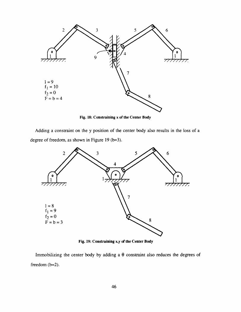
1=9f, = 10
f2 = 0F=b=4
Fig. 18: Constraining x of the Center Body
Adding a constraint on the y position of the center body also results in the loss of a
degree of freedom, as shown in Figure 19 (b=3).
1=8fl =9f2= 0F=b=3
Fig. 19: Constraining x,y of the Center Body
Immobilizing the center body by adding a 0 constraint also reduces the degrees of
freedom (b=2).
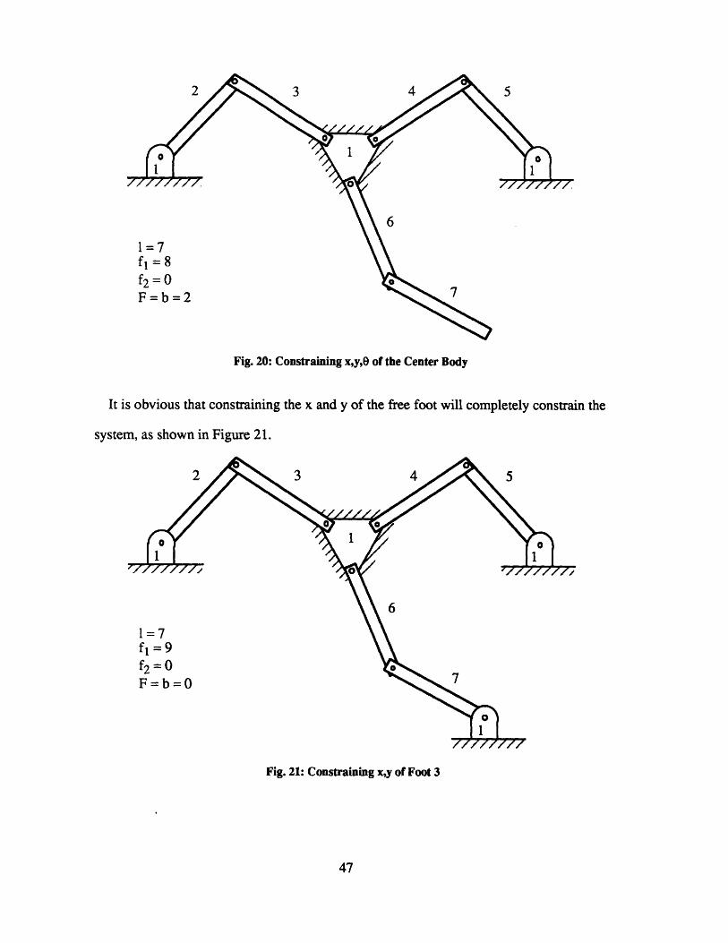
1=7fl= 8f2=0F=b=2
Fig. 20: Constraining x,y,0 of the Center Body
It is obvious that constraining the x and y of the free foot will completely constrain the
system, as shown in Figure 21.
1=7fl=9f2=0F=b=O
Fig. 21: Constraining x,y of Foot 3

So, after constraining the x, y, and theta of the center body, and the x and y of foot 3,
the system has no degrees of freedom (b=O, r=5). This concludes stage one of the
Extended Mobility Analysis.
There are six actuators and only five control variables so far (r = 5, s = 6, so r<s). This
implies that an environmental interaction force or internal force can be controlled, and so
we go on to the second stage of the Extended Mobility Analysis. For climbing between
walls using friction to support its weight, as is the ultimate goal of the LIBRA, it is
desirable to control the horizontal force being applied at the wall by the second foot.
Relaxing the x constraint on foot 2 as shown in Figure 22, the system has one degree of
freedom, and therefore the x force of foot 2 can be controlled.
1=8fl = 10f2= OF=b=l
Fig. 22: Relaxing the x environmental constraint
The system now has six actuators and six control variables. The control vector U looks
like:
ul = [xb,yb,Ob,x 2 ,X3,y 3]T
0////

The LIBRA system with virtual spring-dampers attached to control vector one is
shown in Figure 23. The virtual spring-damper attached to foot 2 is used to control the
force being applied to the ladder in the x direction.
Fig. 23: LIBRA with control vector 1
For the different stages in climbing, different control vectors need to be used. This is
because of the different tasks that the system needs to perform. Control vector one is
used during stages one and three. During stage two, foot 3 is used to support the body,
and foot 2 is lifted and controlled in free space. Control vector two is then used, as given
by:
U2 [XbYbb,x 2 ,Y 2, X3 ]T
2

The LIBRA with virtual spring-dampers attached to control vector two is shown in
Figure 24.
XbodyN.X
INERTIALCOORDINATEFRAME
Foot 3
Fig. 24: LIBRA with control vector 2
Stage four requires foot 3 to support the body, and foot 1 is lifted and moved in free
space. The LIBRA then uses control vector three:
u3 = [x1,yl,xbyb,0bX2] T
The LIBRA with spring-dampers attached to control vector three is shown in Figure
25. Extended Mobility Analyses can be performed on control vectors two and three to
verify that the control vectors are valid. From symmetry, however, it is obvious that they
are.
Y
3

Y
Y1
Ybody
Xbody
2
Fig. 25: LIBRA with control vector 3
4.4: Control equations
The control equations in this section are only derived for control vector one. Similar
analysis will lead to the control equations for the other two control vectors. The six
control variables chosen for control vector one are:
1I = [xb,Yb,0b,X2,X3,Y3]T
The Jacobian matrix, as given by equation (11), is derived in Appendix A for control
vector one. To write the Jacobian explicitly in terms of the joint vector q, the position
constraint on the y direction of foot 2 is solved algebraically and substituted into the
Jacobian.

J(q) =
ax, ax,ae. ae6
aYb aybae ae06
aeb aebae, a06
ax 2 ax2
ae, a06
ax3 ax3
Say3 ay3ael a06
(17)
Since the x2 variable is constrained by the ladder, the force of the foot in the x-
direction is controlled by implanting the commanded control variable into the ladder.
The force equation, as given by (10) is
Xb(cmd) - Xb b(cmd) - Xb
Yb (amd) - yb Yb(md) - Yb
Ob (cmd) - b b (cmd)- ( bF = Kp +KdX2 (cmd) - X2 2 (cmd) - X2
X3(C•d) - X3 X3 (cmd) - i 3
Y 3( cm d) - y3 -y3 (cmd) - y3
(18)
Kp and Kd were chosen to be diagonal, with terms of:
kp = (kpb, kpb, kptheta, kP2, kP3, kP3)
corresponding to the spring constants for each control variable and a similar form for kd.
For the purpose of deriving a gravity compensation term, the mass of the system was
assumed to be at a point at the main body. Although a more detailed gravity
compensation term certainly is possible, computational capability constraints made this
simplifying assumption attractive. This resulted in good experimental results and was

computationally inexpensive. The gravity force due to this lumped mass model is
transformed into joint torques using the transpose of the system's Jacobian matrix. The
gravity term in (12) then becomes:
G(q) = JT[0, M.g, 0,0,0,] T (19)
Combining (12), (17), (18) and (19), the input vector becomes:
T2sT;3
"•4= JT .
Xb (cmd) - Xb
Yb(cmd)- yb
Ob(cmd) - 0 b
X 2 (cmd) - X2
X 3 (cmd) - X 3
y3 (cmd)-- y3
+ Kd
Xb(cmd) - Xb
Yb(cmd)- yb
b(cmd) -- b +x2 (cmd) - x2
X 3 (cmd) - X3
-4(cmd) -
0
M-g
000
Lo
(20)
4.5: Control gain selection
A combination of experimental trial and error and an analysis of a dynamic model of
the LIBRA system was used to select the control gain matrices Kp and Kd. The ranges of
the desired Kp control gains were chosen based on the desired stiffness of the different
virtual spring-damper systems attached to the control variables. The position of the body
is important to control tightly, so the stiffness of the virtual springs on the body is desired
to be high. The feet come in contact with the environment and the forces that they exert
are important to control. By having low stiffness virtual springs, small changes in the
position of the feet due to compliance or sensor error will only have a small effect on the
force being exerted. Therefore the gains on the feet are desired to be fairly low.
4.5.1: Dynamic Model
An analysis of a dynamic model of the LIBRA system assists in selecting the control
gain matrices Kp and Kd. Only the top chain of the LIBRA was modeled, as it is
assumed that the free foot can be analyzed separately. To simplify the model of the
LIBRA, point masses mi are assumed to be located at the positions shown in Figure 26.
Z
/
KP
* * - 1
I/

Ke
m10
Fig. 26: Model of the LIBRA top kinematic chain
where:ml = mass of limb link
m2 = motor mass
m3 = mass of body
m10 = mass of limb three
Ke = environmental stiffness
The limb link masses, which are identical for all links, are assumed to be lumped
halfway along the links. The motor masses are placed at the joints. The body mass is
located at the geometric center of the body. As an approximation, the mass of limb three
is assumed to be at the first joint of the third limb. The actuators are also modeled as
frictionless torque supplies, ignoring the internal friction and actuator dynamics. While
the actuator dynamics are sufficiently fast that they shouldn't affect the dynamics of the
overall system, the friction in the actuators will add a significant amount of damping.
The dynamic equations are derived using Lagrange's equation:
d aT aT - • Sq = 0 (21)dt a4il aq aq
whereT = the kinetic energy of the systemV = the potential energy of the system

To further simplify the equations, it is assumed that the gravity compensation term of
the controller is exact. The equations are linearized about 4 = 0. Appendix C contains
the linearized dynamic equations derived using these assumptions. In state space form,
using the control vector as the state space, these equations can be represented as:
u J(q) -H-' (q -J (q) -K, : J(q) -H-q) (q) -KP u... ...................................... ..... .... ...... +
LI : D u[cmd[J(q) -H-'(q) T (q) -K : J(q) H-'(q)-JT (q) KP ...]
.ucmd . (22)
[Y] = [ 0: I] ...
where H is the configuration dependent inertia matrix
Since the terms of the matrices are not constant, but are instead very configuration
dependent, the system response changes as a function of the configuration.
Equation (22) is linearized around 18 representative configurations of the system.
These points were chosen to reflect the range of motion found in the climbing maneuver.
The xbody position was chosen to be at one half the wall separation of 0.18 m. The 6body
is chosen to be zero, which is the commanded position during the entire climbing gait.
The x2 position of foot 2 is chosen to be at the wall. The only control variable in the top
kinematic chain that really varies during the climbing gait is the Ybody, which was chosen
to vary from -0.22 m through 0.05 m. This represents the fullest possible vertical
movement of the LIBRA in the current climbing setup. Classical root locus methods and
bode plots were used to study the stability of the system. The system gains were chosen
to meet the design specification of a bandwidth of 6 Hz and steady state positioning
errors of the center body of less than 2 mm under a 10 N disturbance. The gains
suggested through this analysis were:

kp =[ 1000,1000, 22, 500]
kd = [160, 160, 4, 120]
After experimental tests, the gains were tuned to:
kp = [1000, 500, 8, 100]
kd = [200, 100, 2, 20]
The dominant poles for these gains, sampled at different configurations, are given in
Figure 27. Appendix C shows the entire pole diagram for these configurations, and the
bode plots of the dominant control variable loops. While it might appear in these
diagrams that the system is under damped and the bandwidth is larger than desired, it is
important to note that the analysis did not include the damping effects of the friction in
the motor gearheads.
Tm
# 1 10A
+ 44 8-
6-
Ybody = 0.0 4-
ybody = -0.1
Ybody = -0.2 2-
0-20 -15 / -10 -5
Ybody = 0.1 Y body = 0.14 -2-
-4-
-6-
-8-
-10i -
0 Re
Fig. 27: Dominant poles of the LIBRA for Ybody from -0.20m -> 0.14 m

The last limb, limb three, was chosen separately to have gains of kp = [100,100] and kd
= [10 10]. This selection was strictly based on experimental trial and error. It was found
that the gains for the third foot have little effect the performance of the upper kinematic
chain. Also, the third foot performance is not sensitive to the gains chosen, and a wide
range of gains could be chosen based on the desired performance of the third foot. Gains
of up to kp = [1000, 1000] and kd = [150 150] were used for closer trajectory tracking.
4.6: Experimental performance
Data from two experiments are presented in the following sections. First, data are
presented for the first stage of the climbing gait including force data gathered from a
force sensor mounted on one of the rungs. Secondly, data are presented for a full
climbing cycle, but no force data was collected. These data are representative of the
performance of the LIBRA under CJTC, and demonstrate the effectiveness of CJTC.
4.6.1: Data from climbing stage one
Figure 28 shows the desired motion for the climbing robot. This is the first stage of the
four stage climbing gait. The trajectory consists mainly of the body's vertical motion
while swinging the third foot over and placing it on a step. Although Ob is not shown in
Figure 28, it is always commanded to be equal to zero. The second foot is pressing
against the step with a commanded horizontal force of 10 Newtons. This force is
specified by moving the commanded control variable x2(cmd) into the wall, at distance of
10N / 100N/m = 0.1 m. Although some compliance exists within the foot and the wall,
the commanded force remains constant by commanding a constant offset distance from
the actual position.

Body CommandedPath
Position
Fig. 28: Desired motion for the climbing robot
Figures 29 and 30 show the trajectory of the main body xb, Yb and Ob positions. The
main body reaches its steady-state position in approximately 4.5 seconds. During the
vertical movement, the xbody (Xb) position varies by as much as 5 mm, but remains within
2 mm once the steady-state position is reached. The Ybody (Yb) control variable followed
the desired vertical motion very accurately as shown in Figure 29, and the steady state
error is almost 0.00 m. After 5 seconds, the third foot has contacted the ladder and is
seating itself, applying forces of up to ten Newtons to the ladder. The center body
location stays close to the commanded position despite this force, which demonstrates the
capability to control manipulation forces and mobility simultaneously. The Obody shows
very small errors, and remains within 3x10 -2 radians, or 1.7 degrees, at all times. The
plateaus seen in Figure 30 are caused by stiction in the inclinometer.

0.20 -
0.15-
0.10-
o 0.05-
o 0.00-
-- 0.05 -m0
-0.10 -
0 1 2 3 4 5 6 7 8 9Time (sec)
Fig. 29: xb, Yb position for a pushup maneuver
-330x10
.0
0 10-
2.O 0-.0
S -10-I.-
-20 -
....................................................... ... ................ ................. .
-· · · ·---; ·---------- ----- ·-
......... Actual theta bodyI,,,,,,," Desired theta bod
0 1 2 3 4 5 6 7 8 9Time (sec)
Fig. 30: Ob for a pushup maneuver
The horizontal foot force of foot 2, shown in Figure 31, stayed within four Newtons of
the commanded force of ten Newtons, even though there is no force feedback. The foot
force varies, as with the xbody, during the vertical motion, but steadies once the
movement is finished. Even when foot 3 is exerting a horizontal force against the ladder,
as occurs after five seconds, the horizontal force from foot 2 stays very close to the
desired force. This demonstrates the capability to control two environmental interaction
forces simultaneously. The force response exceeded the design goals.
.................Xbody position. ... C- .commanded Xbody. ......... .
................ ......... ............. ........ ----------
Commanded Ybod
Ybody positio.n..

.I . . . . . . . . . . . . . . . . . . . . . . . . . . . . . . . . . . . . . .
- Applied x foot forcI........ Desired x foot forc
0 1 2 3 4 5 6 7 8 9Time (sec)
Fig. 31: x2 Force for a pushup maneuver
The third foot contacts the ladder at nearly 4 seconds, and the growing error in x3
shown in Figure 32 is actually a force being applied against the step corresponding to
(error/kp3). The foot is commanded to apply this force on the step to insure a smooth
transition to the next phase of the climbing gait. The y3 positions, not shown here, are
well behaved.
................. ................ T .............. ................... ............ i .............. .I ... ...... ........I........
L.... . ....... .;- ......... .. ........i........:.. ............. ... ................r·--· -- · --- --- ---- -- ·---- -- 1*--
...... ......... ...................... ........ .......... .......*******D siedfeefotx oito
0 1 2 3 4 5 6 7 8 9Time (sec)
Fig. 32: x3 location for a pushup maneuver
60
.. . . . . ... . .
12-
0 10-
z 8-
- 6-0o40 4--
X 2-
... ............................................... ...........................
.. .. . ... . ... . . ... . . ... . .............. ........... ........i........ ................ .........
( 0.50-
E 0.45-
._S0.40
0nn;
' 0.30
u- 0.25LL 0.25
1
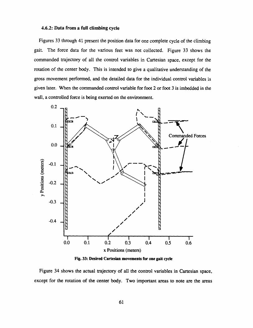
4.6.2: Data from a full climbing cycle
Figures 33 through 41 present the position data for one complete cycle of the climbing
gait. The force data for the various feet was not collected. Figure 33 shows the
commanded trajectory of all the control variables in Cartesian space, except for the
rotation of the center body. This is intended to give a qualitative understanding of the
gross movement performed, and the detailed data for the individual control variables is
given later. When the commanded control variable for foot 2 or foot 3 is imbedded in the
wall, a controlled force is being exerted on the environment.
0.2
0.1
0.0
-0.1
-0.2
-0.3
-0.4
Forces
0.0 0.1 0.2 0.3 0.4 0.5 0.6
x Positions (meters)
Fig. 33: Desired Cartesian movements for one gait cycle
Figure 34 shows the actual trajectory of all the control variables in Cartesian space,
except for the rotation of the center body. Two important areas to note are the areas

where the joint limits were reached. Joint 1 for limb 1 and joint 4 for limb 4 hit hardware
limits during the movement, and the feet were therefore unable to follow the commanded
trajectory. However, the controller continued to function and completed the movement,
demonstrating the robustness of CJTC.
113 Tnnnt 1 1 imlt p•,n-hi-A
0.1
0.0
-0.1
-0.2
-0.3
-0.4
/ /Joint 4 Limit Reached
0.0 0.1 0.2 0.3 0.4 0.5 0.6
x Positions (meters)
Fig. 34: Actual Cartesian movements for one gait cycle
Figure 35 shows the desired and actual positions of the main body for the climb. The
errors are relatively small, and indicate good performance of the system. Figure 36
shows the orientation of the main body for the same climb. While the angle peaks as
high as 8 degrees, it is still acceptable. The small spikes in the commanded position are
artifacts of the planning algorithm.
V.L

0.25
0.20
0.15
- 0.10
S0.05
-. 0.00
" -0.05
-0.10
5 10 15
Time (sec)
Fig. 35: Body movements for one gait cycle
8
. 6
4
2
O -2
-4
-6
5 10 15
Time (sec)
Fig. 36: Body orientations for one gait cycle
Figures 37 and 38 show the x and y positions of all the feet during the climb. The
movements for the individual feet are given later in Figures 39 through 41. In Figure 37,
the ladder step is located at x=0.45m. Even when the foot is pressing against the ladder,
it still appears to move due to the backlash in the actuators and the compliance of the
wheels. The commanded positions above 0.45 m indicate that forces are being
commanded that are proportional to the error signal. In Figure 38, the steps are located at
-0.135m, O.Om and +0.135m. As can be clearly seen, the tracking for both the x and y of
the feet is generally very accurate.

0.6
0.5
0.4
0.3
0
S 0.1o
X 0.0
Stage 2 Stage 3
0 5 10 15 20
Time (sec)
Fig. 37: x positions for all the feet for one gait cycle
0.2
0.1
0.0o
-0.1
-0.2
* -0.3
4 -0.4>b
5 10 15
Time (sec)
Fig. 38: y positions for all the feet for one gait cycle
Figure 39 shows the position data for foot 1. The majority of the time it sits on one
rung, and only moves in Stage Four. Again, note the region where joint 1 was at its limit
of - 117", and the commanded movement was unreachable. Even though it was unable to
follow the x direction trajectory, it still continued to closely track the y direction
trajectory.

0.4
0.3
0.2
"n 0.1
o 0.0
-0.1
0 5 10 15 20
Fig. 39: Foot 1 position vs. time for one gait cycle
Figure 40 shows the position data for foot 2. In Stages 1,3 and 4, it is applying a force
in the x-direction against the rungs that is equal to 100 N/m times the error signal. The
rungs are located at x = 0.45 m, and y = 0 and y = 0.13 m. The small variations in the x
position of the foot while it is pressed against the rungs are due to backlash in the gears
and compliance in the environment. Note the region in Stage 2 where joint 4 was at its
limit of - 117%, and the commanded movement was unreachable. Like foot 1, even
though foot 2 was unable to follow the x direction trajectory, it still continued to closely
track the y direction trajectory.
0.6 Stage 1 Stage 2 Stage 3 Stage 4
0.5
E 0.4
o 0.3
a, 0.2
o 0.1
0.0
5 10 15
Time (sec)
Fig. 40: Foot 2 position vs. time for one gait cycle
I _r

Figure 41 shows the position data for foot 3. In Stage 2 it is applying a controlled
force in the x-direction against the rung that is equal to 100 N/m times the error signal.
The rung is located at x = 0.45 m and y = - 0.13 m. The small variations in the x position
of the foot while it is pressed against the rungs are due to backlash in the gears and
compliance in the environment. In Stage 4 it is resting on a rung located at x = 0.0 m and
y = - 0.13 m. At all times, foot 3 closely tracks the desired trajectory.
Stage 1 Stage 2 Stage 3 Stage 40.6 - ,-- 0.6 - Actual Position
o I I IS0.4 - -- Desired PositionS0.2
0.0
-0.2 - Yfoot3
-0.4
0 5 10 15 20
Time (sec)
Fig. 41: Foot 3 position vs. time for one gait cycle
Looking at the data for a full climb, it is clear that the controller performed well,
tracking the commanded trajectory. Even when joint limits were reached, the controller
still continued to function and track the trajectories of control variables that it was
physically capable of following. Even though force data was not collected it is assumed
that the force was also well controlled.

5: Summary and Conclusions
The Coordinated Jacobian Transpose Control proposed is a viable method for controlling
multiple control variables for both position and force of multilimbed robotic systems in a
unified and coordinated manner. One of its advantages is that it is relatively easy to
implement and can be interfaced with higher level planners and controllers in a
straightforward manner. Also, it is computationally inexpensive and can be run on low
capability processors. The control variables that can be controlled using CJTC are not
restricted to positions of the system. They may be other differentiable functions of the
joint variables, giving the system the ability to control important functions of the system
in a simple fashion. Both mobility and manipulation can be controlled in this fashion. A
methodology called the Extended Mobility Analysis provides a method for choosing an
admissible set of control variables that will not overconstrain the system. Linear analysis
and experimental studies of a three legged climbing robot show that the approach
provides a stable and effective control strategy for both mobility and manipulation for
some mobile multilimbed systems. Good performance was demonstrated experimentally
even though only kinematics and gravity forces were taken into account.

6: References
1Argaez, D.A., An Analytical and Experimental Study of the Simultaneous Control of
Motion and Force of a Climbing Robot, M.S. Thesis, ME Dept., MIT, May 1993.
2Gradetsky, V., Rachkov, M., Uljanov, S., Nandi, G., "Robots for Cleaning andDecontamination of Building Construction," 8th International Symposium on Automation
and Robotics in Construction, Stuttgart, Germany, 3-5 June 1991.
3 Meieran, H., "Frequent Incidents Increase Robot Potential," HAZMAT World, 2(9),
September 1989, pp. 70-73.
4 Nandi, G., Dwivedi, S., Lyons, D., "Climbing Robots for Decontamination of Nuclear
Energy Producing Sites," FAIM 1993 Conference, Ireland, June 28-30 1993
5Potemkin, E., Astafurov, P., Osipov, A., Malenkov, M., Mishkinyuk, V., Sologub, P.,"Remote Controlled Robots for Repair and Recovery in the Zones of High Radiation
Levels," Proceedings of the 1992 IEEE International Conference on Robotics and
Automation, Nice, France, May 1992, pp. 80-82
6Shaffer, G., Stentz, A., "A Robotic System for Underground Coal Mining," Proceedings
of the 1992 IEEE International Conference on Robotics and Automation, Nice, France,
May 1992, pp. 633-638
7Stone, H., Edmonds, G., "Hazbot: A Hazardous Materials Emergency Response Mobile
Robot," Proceedings of the 1992 IEEE International Conference on Robotics and
Automation, Nice, France, May 1992 pp. 67-73
8Woodbury, R., "Exploring the Ocean's Frontiers: Robots and Miniature Submarines take
Oil Drillers to New Depths," Time, December 17, 1990.
9Harmon, S., "A Report on the NATO Workshop on Mobile Robot Implementation,"
Proceedings of the 1988 IEEE International Conference on Robotics and Automation,
Philadelphia, PA, April 1988, pp. 604-610
10Meieran, H., Gelhaus, F., "Mobile Robots Designed for Hazardous Environments,"
Robotics Engineering, Vol. 8, March 1986, pp. 10-16

11 Raibert, M., Brown, H., Chepponis, M., "Experiments in Balance with a 3D One-
Legged Hopping Machine," The International Journal of Robotics Research, Vol. 3, No.
2, 1986, pp. 75-92
12Brooks, R. A. and Flynn, A. M., "Rover on a Chip," Aerospace America, Vol. 27, No.
10 Oct 1989, pp. 27-36
13 Pugh, D., Ribble, E., Vohnout, V., Bihari, T., Walliser, T., Patterson, M., Waldron, K.,
"Technical Description of the Adaptive Suspension Vehicle," The International Journal
of Robotics Research, Vol. 9, No. 2, April 1990, pp 24-42.
14Saito, F.; Fukuda, T.; Fumihito, A., "Swing and Locomotion Control for a Two-Link
Brachiation Robot," Control Systems, Vol. 14, No. 1, February 1994, pp. 5-12
15 Puttr6, M., "Undaunted Dante readies for Inferno," Mechanical Engineering, December
1993, pp. 58-59
16Bares, J.; Hebert, M.; Kanade, T.; "AMBLER, an Autonomous Rover for Planetary
Exploration," Computer, Vol. 22, June 1989, pp. 18-26
17S.M. Song and K.J. Waldron, Machines that Walk: The Adaptive Suspension Vehicle,
MIT Press, October 1988.
'8Gorinevsky, D., Shneider, A., "Force Control in Locomotion of Legged Vehicles over
Rigid and Soft Surfaces," The International Journal of Robotics Research, Vol. 9, No. 2,
April 1990, pp. 4-23
19McGhee, R., Iswandhi, G., "Adaptive Locomotion of a Multilegged Robot over Rough
Terrain," IEEE Transactions on Systems. Man Cybernetics, Vol. 9, No. 4, pp 176-182
2 0Sutherland, I., Ullner, M., "Footprints in the Asphalt," The International Journal of
Robotics Research, Vol. 3, No. 2, 1984, pp. 29-36
2 1Brooks, R., "A Robot that Walks : Emergent Behaviors from a Carefully Evolved
Network," Proceedings of the 1989 IEEE International Conference on Robotics and
Automation, Scottsdale, USA, May 1989, pp. 692

22Lee, T., Shih, C., "Real Time Computer Control of a Quadruped Walking Robot,"
Journal of Dynamic Systems, Measurement, and Control, Vol. 108, December 1986, pp.
346-354
23Hirose, S., Masui, T., Kikuchi, H., "Titan III: A Quadruped Walking Vehicle,"Proceedings of the 2nd ISSR Symposium, Tokyo, Japan, 1984, pp. 247-253
24Luk, B., Collie, A., Bingsley, J., "Robug II: An Intelligent Wall Climbing Robot,"
Proceedings of the 1991 IEEE International Conference on Robotics and Automation,Sacramento, CA, April 1991, pp. 2342-2347
25Neubauer, W., "Locomotion with Articulated Legs in Pipes or Ducts," Robotics andAutonomous Systems, Vol. 11, 1993, pp. 163-169
2 6Gradetsky, V. and Rachkov, M., "Wall Climbing Robot and Its Applications for
Building Construction," Mechanical Systems Engineering, 1990, pp. 225-231
27Nagakuba, A. and Hirose, S., "Walking and Running of the Quadruped Wall-ClimbingRobot," Proceedings of the 1994 IEEE International Conference on Robotics and
Automation, San Diego, Vol. 2, May, 1994, pp. 1005-1013
2 8Byrd, J.S., and De Vries, K.R., "Six-legged Telerobot for Nuclear Applications
Development, The International Journal ofRobotics Research, Vol. 9, No. 2, April 1990,
pp. 43-52
29Foster-Miller, Inc., 350 Second Ave., Waltham, Massachussets, 02154-1196
30Klein, C. A.; Olson, K. M. and Pugh, D. R., "Use of Force and Attitude Sensors for
Locomotion of a Legged Vehicle", International Journal of Robotics Research, Vol. 2,
No. 2, 1983, pp. 3-17
31Gardner, J., Srinivasan, K., Waldron, K., "Closed Loop Trajectory Control of Walking
Machines," Robotica, Vol. 8, 1990, pp. 13-22
32Gardner, J., "Force Distribution in Walking Machines over Rough Terrain," Journal of
Dynamic Systems, Measurement, and Control, Vol. 113, December 1991, pp. 754-758

33Gardner, J., Srinivasan, K., Waldron, K., "A Solution for the Force Distribution
Problem in Redundantly Actuated Closed Kinematic Chains," Journal of Dynamic
Systems, Measurement, and Control, Vol. 112, September 1990, pp. 523-526
34Khatib, O., "Motion/Force Redundancy of Manipulators, " American Symposium on
Flexible Automation, Kyoto, Japan, 1990
35 Raibert, M.H. and Craig, J. J., "Hybrid Position/Force Control of Manipulators",
Journal of Dynamic Systems, Measurement and Control, June 1981, pp. 126-133
36Yoshikawa, T. and Zheng, X., "Coordinated Dynamic Hybrid Position/Force Control
for Multiple Robot Manipulators Handling One Constrained Object, " The International
Journal of Robotics Research, Vol. 12, No. 3, MIT, 1993, pp. 219-230
37Asada, H and Slotine, J.-J. E., Robot Analysis and Control, Wiley-Interscience, 1986
38Hogan, N., "Impedance Control: An Approach to Manipulation: Part I--Theory, Part II-
-Implementation, Part III--Applications," Journal of Dynamic Systems, Measurement and
Controls, March 1985, pp. 1-24
39Hogan, N., "Impedance Control of Robots with Harmonic Drive Systems," Proceedings
of the 1991 American Control Conference, Boston, MA, June 1991
40Schneider, S.A. and Cannon, R. H. Jr., "Object Manipulation Control for Cooperative
Manipulation: Theory and Experimental Results," IEEE International Conference on
Robotics and Automation, Vol. 8, No. 3, June 1992, pp. 383-394
41Schneider, S.A. and Cannon, R. H. Jr.; "Experimental Object-Level Strategic Control
with Cooperating Manipulators," International Journal of Robotics Research, Vol. 12,
No. 4, August 1993, pp 338-350
42 Mills, J., Lokhorst, D., "Stability and Control of Robotic Manipulators During
Contact/Noncontact Task Transition," IEEE Transactions on Robotics and Automation,
Vol. 9, No. 3, June 1993, pp. 335-345
43 Papadopoulos E. and Dubowsky S., "On the Nature of Control Algorithms for Free-
Floating Space Manipulators," IEEE Transactions on Robotics and Automation, Vol. 7,
No. 6, December 1991, pp. 750-758

44Hootsman, N.A.M., Motion Control of Manipulators on Mobile Vehicles, Ph.D. Thesis,
ME Dept., MIT, January 1992
45 Hootsmans, N. A. M. and Dubowsky, S., "Control of Mobile Manipulators Including
Vehicle Dynamic Characteristics," Procceedings of the Fourth Topical Meeting on
Robotics and Remote Systems, February 24-28, 1991.
46 Seraji, H., "Configuration Control of Redundant Manipulators: Theory and
Implementation, " IEEE Transactions on Robotics and Automation, Vol. 5, No. 4, August
1989, pp. 472-490
47Seraji, H., "An On-line Approach to Coordinated Mobility and Manipulation,"
Proceedings of the 1993 International Conference on Robotics and Automation, pp 28-33
48Lim, D.; Lee, T. and Seraji, H.,"A Real-Time Control System for a Mobile Dexterous 7
DOF Arm," Proceedings of the 1994 IEEE International Conference on Robotics and
Automation, San Diego, Vol. 2, May, 1994, pp. 1188-1193
49Papadopoulos, E. and Dubowsky, S., "Failure Recovery Control For Space Robotic
Systems," Proceedings of the 1991 American Control Conference, Boston, MA, June 26-28, 1991. Invited.
50Craig, J. J., Introduction to Robotics Mechanics and Control, second edition, Addison
Wesley, 1989
5 1Morel, G., Programmation et adaptation de l'impidance de manipulateurs au contact,
Ph.D. Thesis, L'Universite Pierre et Marie Curie, June 1994
52Duffy, J., Analysis of Mechanisms and Robot Manipulators, Edwards Arnold Ltd.,
London, Great Britain, 1980
53Sandor, G.; Erdman, A., Advanced Mechanism Design: Analysis and Synthesis, Volume
2, Prentice-Hall, Inc., New Jersey, 1984
54Escap Motion Systems Catalog, 1991. Portescap US Inc., 36 Central Ave., Hauppauge,
NY, 11788
55Delta Tau Data Systems, Inc., 21119 Osborne St., Canoga Park, CA, 91304

Appendix A: LIBRA Jacobian Equations
Derivation of the Jacobian for the LIBRA
xbdy = 2L -cos(0) + 2L -cos(O + 01) + r cos(O + 01 + 92 -6)6
Ybody = 2L. sin(l)+ 2L -sin(Q + 01)+ r sin(O + 0 1 +02 -7)6
Obody = + 1I + 02
Xfoot = 2L[cos(p) + cos(q + 01) + cos(q + 01 + 02+) COs(O + 01os( + 2 + 3 + 4)] +N cos(q + 01 + 02)
Xfree = Xbody + r -sin(O + 01 + 02) + 2L sin(4 + 01 + 2 + 05) + 2L -sin(Q + 01 + 02 + 05 4Yfree = Ybody - r cos(4 + 01 + 02) - 2L cos(+ + 01 + 02 + 05)- 2L cos(O + 01 + 02 + 05
to derive phi using the y position constraint on foot 2:
y = sin(0)[2L + 2L c, + 2L c12 +2L*c123 + N. c12]+cos(0)[2L23 + 2L s 234 + N s12 ]
let k, = 2L + 2L-c, + 2L- c23 + 2L-c1234 + Nc 2k2 = 2L s, + 2L s3 + 2L .sl234 + N. S12
y = sin(0) ki + cos() -k2 = 2u +1- u2
1+u 2 2k2 +1+ 2
u=kl +k _y2
y+k 2
2,, + yk2

let :
X bo dyYbody
Obody
Xfoot
Xfree
Yfree
Jacobian = U,60'
Terms of the Jacobian:
6 Xbody
6802
= (-2L. so - 2L -s 1
= (-2L -s - 2L -sol
= (-2L -so - 2L -So,
- r s012 -n/6)
- r -S012-n/6 )
1+ do+ 2L -s
do -rS12-n/6
6Xbody
/13 803
114 dy -2L. -s804
115 =0116 =0
- 2L so - r S 12- /6
121 ody = 2L-c+2L.ci+r-c12 +6) 1+ -2L.c,121 - = 0 c 1- 2L
J22 = '5 2 Lc, + 2L cj + -c12-
6yy (2L- C, + 2L -c, + r 'c1 dIJ2 03d0
S124= dy (2L-c, + 2L-c+c,r12-.16 {(
125 = 0
126 = 0
03
O4
95
_96
-r2
T=T4-'r
'I = 'imp
_ Xbody
501
112 =
- S12-r /6
r'p__ 1"

J31= 68body d4
601 d0e
36 body d4132 1 + d602 d02
J33 = 68body d-
34 -= 8body - d4
80 body135 = = 0885
60611 6 xf°°t =2 22 LN d4
J41 -2L "s - 2s - 2-s -2L- -S¢12L12342 1 + 2L- so
42 foot -2L-2s-2L -s 123 -2s123 -2L 1234 -N4S12(1+ +2L-s-
043 = = -2L -s - 2L -so - 2L. sO123 - 2L -s1234 - N S012 _ 2L -S123 -
J44 x f t = (-2L -s - 2L -s -2L - 123 -2L -S1234 - N S12 )- 2L S1234
145 = 0
146 = 0
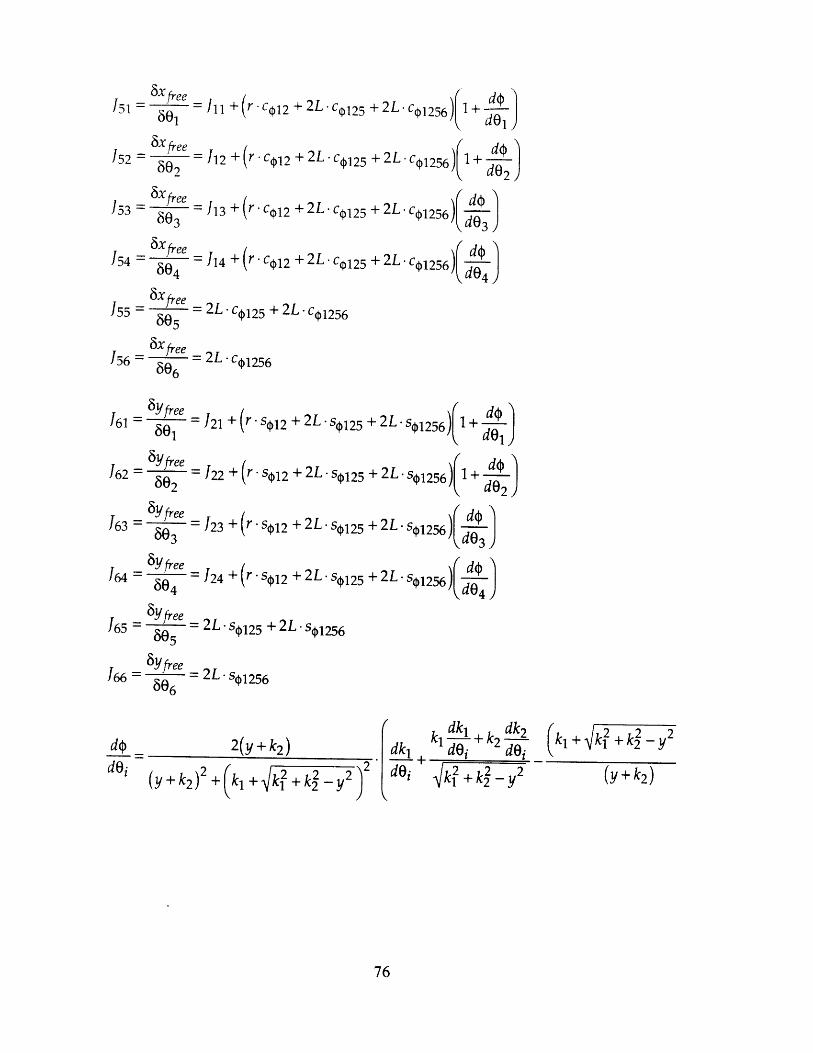
J51 6xfee Ill +(r
J52 602 J12 +- (r
153- ee = 13 + "r -603
J54= 6Xfree 1 J14 +(r.6046xe
c0 12 + 2L -c 125 + 2L 1256)1 +
c012 + 2L -c0 125
c•12 + 2L -C 125
C01 2 + 2L. C-125
x freeJ55 = 8 2L' C125 + 2L C1256
6x6X freeJ56 = 06 2L c012566()6125
do
dO1)
+2L c12561
+ 2L -co1256) dd3
+ 2L . c1256 4
6- Yfree =
601
-Y 6 free
16 3
64 - free14 604
J21 + (r S012
122 + (r s S12
123 + (r -S12
+ 2L- s 125 + 2L .
+ 2L * s0125 + 2L -
+ 2L -S0125 + 2L -
124 + (r' 12 + 2L. S0125 + 2L
j( doS01256( d3
dS4
6 - y free
165 = 805 = 2L s0125 + 2 L' S 125 6
J66 = = 2L s012566806
do _ 2(y+k 2 )di (y + k2 2 + ( k1 + k, +2 + ky2
d kl ki + k-2 iklk 2 +k k y2k + k2 2 +k 2
dAi k2 +k- y2 (y + k 2)
81256)(1+ dop
d02
doS01256) d1)
-

Appendix B: Power Amplifiers
Voltage to current amplifiers were custom built for the LIBRA project. They are
powered by two Zytec 24 volt power supplies I hooked in parallel to provide a driving
voltage range from - 24 volts to + 24 volts, and an amperage of up to 6 amps, continuous.
The hearts of the amplifiers are LM12CLK linear power operational amplifiers,
manufactured by National Semiconductor 2. Linear amplifiers, rather than pulse width
modulated amplifiers are used for their simplicity, even though PWM amplifiers would
be much more power efficient. Trimpots are used to tune the amplifiers to a uniform
gain. The voltage offset is adjusted from the PMAC. Unfortunately, the PMAC tends to
drift in its output signal, requiring periodic testing and adjustment every month.
Voltage to current amplifiers are used to make the motors behave as torque servos.
The characteristic equation of the amplifier-motor circuit shown in Figure B 1 is:
(2-R, + R3 + R4 ).s + 1
in (R3 + R,) Lm s2 + [R, (R4 + Rm - R3) + Rm-R 3]s + R
Using the appropriate values for the various elements, the time constant of the
amplifier-motor system is 1.52 microseconds, resulting in a bandwidth of 656 Hz. Since
this is much higher than the bandwidth of the controller, for the purposes of this thesis the
amplifier-motor system can be considered to be an ideal torque servo system. It is
important to note that this does not include the damping effects of the friction in the
motor gearheads.

:2I
r
KV
L, 4 - IVVV ý..I, .. jVl..
D = Harris A 15A rectifiersHeat sinks required
Fig. BI: Power amplifier schematic
2--
2
F-

Amp I Amp 4
RS I
I Trimpot
Trimpot
I IC I M
I r•-• re-1 Cl -I_ = - -- - j
I Trimpot I I
RS I
I I 1 1 1 I
LM12CLK
LM12CLK
> I
S Trimpotz
Jc~o I Dl
C R4El I___________ I_
I =2I Trimpot II
I Trimpot
Amp 3
Fig. B2: Power Amplifier Card Layout
I
1I
II
Amp 1I Amp 4
SI_ _ _I
I I)I I I I)1 I
II K7 1
II
III
I
1II
RSI ts 0 Ir•5 r•l rR4r
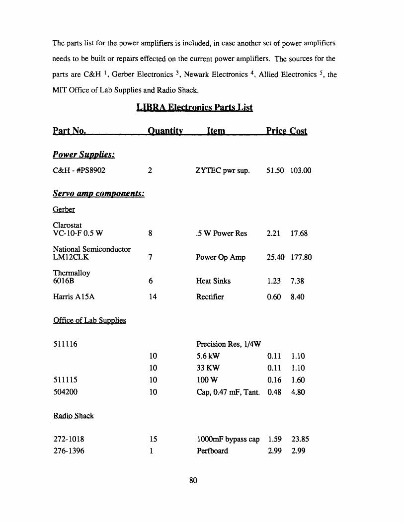
The parts list for the power amplifiers is included, in case another set of power amplifiers
needs to be built or repairs effected on the current power amplifiers. The sources for the
parts are C&H 1, Gerber Electronics 3, Newark Electronics 4, Allied Electronics 5, the
MIT Office of Lab Supplies and Radio Shack.
LIBRA Electronics Parts List
Quantity
Power Supplies:
C&H - #PS8902
Servo amp components:
Gerber
ClarostatVC-10-F 0.5 W
National SemiconductorLM12CLK
Thermalloy6016B
Harris A15A
6
14
Item
ZYTEC pwr sup.
.5 W Power Res
Power Op Amp
Heat Sinks
Rectifier
cirP
Cost
51.50 103.00
2.21 17.68
25.40 177.80
1.23
0.60
7.38
8.40
Office of Lab Supplies
Precision Res, 1/4W
5.6 kW
33 KW
100W
Cap, 0.47 mF, Tant.
Radio Shack
1000mF bypass cap 1.59
Perfboard 2.99
Part No.
511116
511115
504200
0.110.11
0.160.48
1.10
1.10
1.60
4.80
272-1018
276-1396
23.85
2.99
Part N0

276-147 1 PC Board 3.79 3.79
271-343 9 10K trimmers 1.49 13.41
Connection components:
(1): 29 encoder lines from Ascender to the junction panel.
37 pin D-sub connectors, connected by a 37 line flat ribbon cable.
2 male ribbon connectors and 2 female receptacles required. A wire wrap rec.will be used on the junction panel, but the connector for the LIBRA has yet to befinalized.
Newark:
Stock No. 81F5186 2 req'd rec 14.45 28.90Stock No. 81F5025 3 req'd ribbon plugs 6.73 20.19
(2): 12 motor lines from junction panel to ascender.
1 12 line cable, using reverse sex circular plastic connectors.
2 plugs are required for the cable, and 1 receptacle each for the junction panel andthe Ascender. 14 pin connectors will be used.
Allied:
Stock No. 512-1172 3 req'd plug 2.28 11.40StockNo. 512-1173 4req'd rec 1.85 11.10Stock No. 512-1210 1 req'd 100pins 19.00 19.57Stock No. 512-1215 1 req'd 100 sockets 22.00 22.94
(3): 3 power lines from junction panel to servo amps.
Heavy-duty nylon interlocking connectors.
Radio Shack:274-152 1 req'd male 1.69 1.69274-155 1 req'd female 1.69 1.69
(4): 6 PMAC control lines from junction panel to servo amps.
1 line, 15 pin D-sub connectors.
The cable will only need 1 connector, as the end coming from the junction panel
will come directly off of the 50 pin PMAC connector. The other end of the cable will
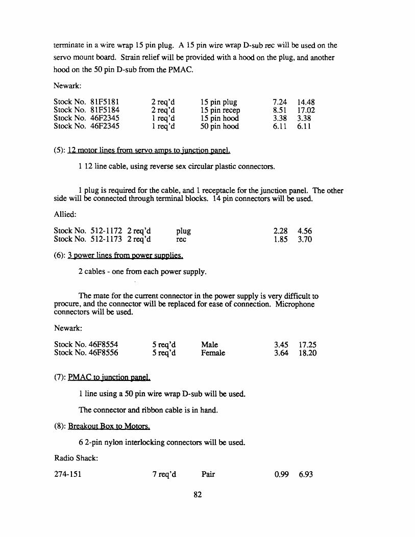
terminate in a wire wrap 15 pin plug. A 15 pin wire wrap D-sub rec will be used on the
servo mount board. Strain relief will be provided with a hood on the plug, and another
hood on the 50 pin D-sub from the PMAC.
Newark:
Stock No. 81F5181Stock No. 81F5184Stock No. 46F2345Stock No. 46F2345
2 req'd2 req'd1 req'd1 req'd
15 pin plug15 pin recep15 pin hood50 pin hood
(5): 12 motor lines from servo amps to junction panel.
1 12 line cable, using reverse sex circular plastic connectors.
1 plug is required for the cable, and 1 receptacle for the junction panel. The otherside will be connected through terminal blocks. 14 pin connectors will be used.
Allied:
StockNo. 512-1172 2req'dStockNo. 512-1173 2req'd
plugrec
2.28 4.561.85 3.70
(6): 3 power lines from power supplies.
2 cables - one from each power supply.
The mate for the current connector in the power supply is very difficult toprocure, and the connector will be replaced for ease of connection. Microphoneconnectors will be used.
Newark:
Stock No. 46F8554Stock No. 46F8556
5 req'd5 req'd
MaleFemale
3.45 17.253.64 18.20
(7): PMAC to Junction panel.
1 line using a 50 pin wire wrap D-sub will be used.
The connector and ribbon cable is in hand.
(8): Breakout Box to Motors.
6 2-pin nylon interlocking connectors will be used.
Radio Shack:
0.99 6.93
7.248.513.386.11
14.4817.023.386.11
274-151 7 req'd Pair

(9): Breakout Box to Encoders.
10-pin DIP connectors will be used
Newark:
Stock No. 46F730 12 req'd
CABLING:
100 Feet of 24AWG 12 wire cable
Newark:Stock No. 44F3506WA 100 ft 6-pair cable 62.62 62.62
100 Feet of 37 line ribbon cable
Newark:Stock No. 36F661WA 100 ft 80.38 80.38
20 Feet of 16AWG stranded 2 wire cable
Radio Shack:278-1105 30 ft 4.99 4.99
1 AC power plug for power supplies (1 already in hand)
Radio Shack:278-1257 1 req'd 6 foot cable 3.99 3.99
Total Cost:$763.51
male 2.96 35.52

Appendix C: Gain Selection
The dynamic model was derived using Lagrange's equations. The equations are
linearized about various positions, with the velocity equal to zero. This allows
simplification of the equations. The friction in the gearheads, which is difficult to
characterize, is not included in the dynamic model. This means that the analysis will
show less damping than the actual experimental system.
The LIBRA system is analyzed using the model shown in Figure 24. The figure is
repeated here for convenience:
m2 m2
Ke
ml0
Fig. Cl: Model of the LIBRA
The masses used are given as:
ml = 0.1960 kg
m2 = 0.3466 kg
m3 = 1.00 kg
ml0 = 1.09 kg
Ke = 5837 N/m
The length of each link is given as 2-L, where L is specified as:
L = 0.078 m
The distance from a motor mounted on the body to the center of body is given as:
r = 0.048 m

The distance from a motor mounted on the body to another motor mounted on the body is
given as:
N = 0.083 m
The LIBRA positions (xb, yb, Ob, x2) are given by:
xb = 2-L-(cos(o) + cos(0+01)) + r-cos(0+01+02-1c/6)
Yb = 2.L.(sin(0) + sin(0+8 1)) + r-sin(0+01+02-r1/6)
Ob= 0+01+02
x2 = 2.L-(cos(+0 1)+cos(0+ 1)+cos(0+ 1+02+0 3 )+cos(+01 +02+03+04)) +N-cos(0+01+02)
Define the inertia matrix M as:
cO cl c2 c3 c4
dO dl d2 d3 d4
M = e0 el e2 e3 e4
fO fl f2 f3 f4
gO gl g2 g3 g4
where:
cO = 24.ml.L 2 + 26-m2-L2 + 6.(m3+ml0).L 2 + m3.i 2 + 2.(ml+m2)-N2 + ml0.N2
cO = cO + L2 .cos(2.0+01)-(10.ml+12-m2+4 -m3+4 .m10)
cO = cO + 2.m3.L-r.(cos(2.0+01 +02-7n/6)+cos(2.0+2.01+02-7r/6))
cO = cO + 2-ml -L.*N(cos(2.0+01+02-7t/3)+cos(2.0+2.01+02-1t/3))
cO = cO + 4.(m l+m2)'L*N'(cos(2"0+01+02)+cos(2"0+2-01+02))
cO = cO + (6.m 1+4m2)'L 2 .(cos(2-0+01+02+03)+cos(2.0+2-01+02+03))
cO = cO + (3-ml+2-m2)-L-N-(cos(2.0+2-01+2-02+03))
cO = cO + 2-ml-L2-(cos(2.0+01+02+03+04)+cos(2.0+2.01+02+03+04)+
cos(2.0+2.01+2.02+2.03+04))
cO = cO + ml-L.N.cos(2i+2.0+2 2.02+03+04)

cl = 15-mi-L 2 + 16-m2-L 2 + 4.(m3+ml 0)-L2 +
(5-ml+6.m2+2-m3+2.m10).L 2.cos(2-0+01)
cl = cl + m3-r2 + m3-L-r-(cos(2-+0l1+02-7t/6) + 2-cos(2-0+2-81+02-t/6))
cl = cl + m10.N 2 + ml0-L-N-(cos(2-P+01+02-7t/3) + 2-cos(2*.+2.01+02-2t/3))
cl = c + 2.(ml+m2)-N2 + 2.(ml+m2)-L.*N(cos(2i.+01+02) + 2-cos(2.4+2-01+02))cl = c + (3-ml+2-m2).L 2-(cos(2.-+01+02+03) + 2-cos(2·.+2-01+02+03))cl = cl + (3.ml+2-m2).L.N.cos(2.0+2.01+2-02+0 3)c 1 = cl + m 1.L2.(cos(2.0+01 +E2+03+04)+2.cos(2.0+2.01 +02+03+e4)+
2-cos(2.0+22.01+2.2 +2+03+04))cl = c + m-L-N-~cos(2.04+2*O+1+202+03+04)
c2 = 6-ml-L 2 + 4-m2-L2 + m3-r + ml0.N2 + 2.(ml+m2).N 2
c2 = c2 + m3-L.r.(cos(2-04+1+02-1/6)+cos(2.0+2-01+02-r/6))
c2 = c2 + ml0-L-N-(cos(2-0+0 1+02-7r/3)+cos(2.0+2-01+62-2t/3))
c2 = c2 + 2-(ml+m2).L.N-(cos(2.0+01+02)+cos(2-+2.01+02))
c2 = c2 + (3.m +2-m2).L 2 .(cos(2"0+01 +02 +03 )+cos(2-0+2.0 1 +02 +03))c2 = c2 + (3.ml+2-m2).L*N-cos(2-0+2-01+2-02+03)
c2 = c2 + ml.L2.(cos(2.0+01+02+03+04)+cos(24.+2.01+02+03+04)+
2.cos(2.0+2-1 +2.02+2+2.3+04))
c2 = c2 + m-L-LN-cos(2-p+2*9l+2.02+03+0 4)
c3 = 4-m2-L 2 + 6-ml-L 2 + (3-ml+2-m2).L 2 .(cos(20+01+02+03)+cos(2-0+2.01+02+03))
c3 = c3 + (1/2).(3.ml+2.m2)*L*N.cos(2.0+2-01+2.02+03)
c3 = c3 + ml L2.(cos(2-.+01 +02+03+04)+cos(2.0+2.01+02+03+04)+
2-cos(2"0+2.01+2-02+2-03+04))
c3 = c3 + (1/2).ml.L.N.cos(2.0+2-01+2-02+03+04)
c4 = ml.L 2 .(1 +cos(2-+01+02+03+04)+cos(2-0+2.01+02+03+04)+
cos(2.0+2.01+2-02+2-03+04))
c4 = c4 + (1/2).ml-L*N-cos(2.0+2*01+1+22+03+04)
dO = 15-mi-L2 + 5-ml.L 2.cos(20+01) + (8-m2+2-m3+2.m10).L 2.(2 + cos(2-+01)) +
m3.r 2
dO = dO + ml0-N2 + 2-(ml+m2).N 2 + m3L.r-(cos(2.+601+02-7r/6)+
2-cos(2-4+22-01+02-7r/6))
dO = dO + ml0o-LN-(cos(2-0+01+02-1r/3) + 2-cos(2-0+2-01+02-7r/3))

dO = dO + 2.(mi + m2)-L.N.(cos(2.0+0 1+62) + 2 -cos(24.+2 -0 1+02))dO = dO + (3-ml + 2-m 2)-L2 .(cos(2-0+01+02+0 3) + 2-cos(2-0+ 2 .01+02+03))dO = dO + (3-mi + 2-m 2).-L-Ncos(2-0+2-. 1+2-6 2+03)dO = dO + mi -L2 .(cos(2.0+0 1 +02+0 3+04)+2-cos(2.0+2.01+02+03+04)+
2-cos(2-0+22-0+22 +2+-03+04))dO = dO + mi-L*N-cos(2.0+2.0 1+2.0 2+03+04)
dl = 15-ml-L 2 + (4.m2+m3+ml0).4.L 2 + m3-r2 + ml 0.N2 + 2.(mI+m2).N 2
dl = dl + 2-m3-L-r-(cos(2-.+2-. 1+02-1t/6)) + 2-ml10 -LN-cos(2.0+2.01+0 2-rt/3)
dl = dl + 4-(ml+m2)-L*N-cos(2-0+2-01+0 2 ) + (3.ml+2.m2)-2-L 2.cos(24+2.01+0 2+03)dl = dl + (3.ml+2.m2)-L-N-cos(2.0+2.01+2.0 2 +03) +
ml -L"N-cos(2-0+2-8 1+2-02+03+0 4)dl = dl + 2-ml.L 2.(cos(2.0+2.0 1+02+0 3+04 ) + cos(2"0+2"01+2.02+2.03+04))
d2 = m3.r 2 + m10 .N2 + 2-(ml+m2).N 2 + 6.ml.L 2 + 4-m2-L 2
d2 = d2 + m3-L-r-cos(2-0+2-6 1+02-nt/6) + m1o-L-N-cos(2-0+2-6 1+02-Xr/3)
d2 = d2 + 2-(ml+m 2 )-L-N.cos(2.0+2-0 1+02) + (3-ml+2.m2)-L 2 .cos(2-4+2.01+0 2+03)d2 = d2 + (3-ml+2.m2).L.N-cos(2-0+2-01+2.0 2+03) +
ml -L-N-cos(2"0+2-01+2'02+03+04)d2 = d2 + ml.L2.(cos(2.0+2-0 1+02 +03+0 4 ) + 2-cos(2.0+2.01+2-02+2.03+04))
d3 = 6-ml-L 2 + 4.m2.L2 + (1.5-ml+m2).(2.L 2.cos(2±+2.01+02+0 3)+L*N-cos(2.+2-0 1 +2.02+03))
d3 = d3 + milL 2-(cos(2-0+2.01+0 2+03+04 ) + 2-cos(2.0+2.0 1+2.0 2+2-03+0 4 ))d3 = d3 + (1/2)-ml-L-N-cos(2.0+2.0+1+20 2+03+04 )
d4 = ml-L 2 + ml.L2 .(cos(2.+2.0 1+02+63+0 4) + 2-cos(2-0+2-01+22+23+04))d4 = d4 + (1/2)-mlL*-N-cos(2-0+2.0 1+2-02+03+04)
e0 = m3-r2 + ml0-N2 + 2.(ml+m2).N 2 + 6-ml-L2 + 4-m2-L2
eO = e0 + m3-L-r-(cos(2-04+1+02-nr/6) + cos(24.+2.01+02-rt/6))e0 = e0 + mlo-L-N-(cos(2-04+ 1+02-xt/3) + cos(2.0+2.01+02-t/3))
e0 = eO + 2-(ml+m2)-L-N-(cos(2-0+01+02) + cos(2-0+2.0 1+02))e0 = eO + (3-m l+2m2)-(L2.cos(2"0+01 +2+0 3)+L2.cos(2"0+2"01+02+03)+
L.N-cos(2-0+2-61+2-02+03))eO = eO + m i.L 2-(cos(2.-0+1+02+0 3+04)+cos(2.0+2-0 1 +2+03+04)+
cos(2-0+2-01+2+2-82+203+4)) + ml-L*N-cos(24.+2.0 1+2-. 2 +03 +04)

el = m3-r 2 + ml0.N 2 + 2.(ml+m2)-N2 + 6.mi.L2 + 4.m2.L 2
el = el + m3-L-r-cos(2-P+2-l+062-1n/6) + m10i-LN.cos(2-.+2-01+0 2-jc/3)
el = el + 2-(mI+m2).L.N-cos(2.4+2-81+02)
el = e 1 + (3-m 1+2.m2)-(L 2 .cos(2.4+2.01+02+03)+L.N.cos(2.-+2.01+2.0 2+03))el = el + m .L.(L-cos(2.4+2.1 +02+03+04)+N-cos(2.0+2-.1+2-02+03+04)+
2-L-cos(2*.+2.01+2.02+2-03+04))
e2 = m3-r 2 + ml0.N2 + 2.(ml+m2)-N2 + 6-ml-L2 + 4-m2-L2
e2 = e2 + (3.ml+2-m2)-L*N-cos(2.-+2-01+2.02+0 3)e2 = e2 + ml.(L-N-cos(2*.+2*01++2.02+3+04) + 2.L 2.cos(20+2.0 1++2.2+2.03+04))
e3 = (1/2).(3.ml+2.m2)-L-N-cos(2*.+2.01+2.02+0 3) + 6-ml-L 2 + 4-m2-L 2
e3 = e3 + (1/2).ml.(L-N-cos(2*.+2-0l+2.z2+0 3+04 ) +
4-L 2.cos(2*.+2*0+1+2-2+2.03+0 4 ))
e4 = ml-L2 + (1/2).ml.(L*N-cos(20+2.01+2.02+03+0 4) +
2.L 2.cos(2.0+2.01+2-02+2-63+04))
fO = 6-ml-L 2 + 4-m2-L2 + (1/2).(3-ml+2.m2).L-N-cos(2ý+2.01+2-. 2+0 3)
fO = fO + (3.ml+2.m2).L 2.(cos(24+01+02+03)+cos(2-.+20.1+02+03))
fO = fO + ml-L2-(cos(2-0+01+02+0 3+04 ) + cos(2.0+2.01+02+03+04) +
2-cos(240+2-61+2*62+2+2-03+04))
fO = f0 + (1/2)-ml*L-N-cos(2-4+2.01+2.02+03+04)
fl = 6-ml L2+4-m 2-L2+(1/2).(3.ml+2.m2).(2-L 2 .cos(20+2.01+02+03)+L-N-cos(2-0+2.01+2-0 2+03))
fl = fl + ml-L2.(cos(2-.+2.01+0 2+03+04 ) + 2-cos(24.+2.01+2.02+2.03+04))fl = fl + (1/2)-ml.L-N-cos(2-0+2.0 1+2-02+0 3+0 4)
f2 = 6-ml-L 2 + 4-m2-L2 + (1/2)-(3-m1+2-m2).L.N.cos(20+2.01+2-0 2 +0 3)f2 = f2 + (1/2)-ml-(L-N-cos(2.0+2.01+2-02+03+04) + 4-L2 .cos(24.0+2* 1+1+2.0 2+2 3+04 ))
f3 = 6-mi-L 2 + 4-m2-L2 + 2-ml-L 2 -cos(20+2-0++2.02+2.0 3+0 4)
f4 = ml-L2 + ml.L2 .cos(2.+2.01+2.02+2-0 3 +04 )

gO = ml.L2 -(1 + cos(2.0+01+02+03+0 4) + cos(2'.+2-01+02+03+0 4) +cos(24.+2-01+2202+2.03+04))
gO = gO + (1/2).ml-L-N-cos(2.-+2-01+2-02+03+04)
gl = ml L-(L+L.cos(2.0+2.01+02+03+0 4)+( 1/2).N.cos(2.+2.0 1+2.02+03+04)+L-cos(2-4±2-0+21+22+2"03+0 4))
g2 = ml-L.(L + (1/2)-N-cos(2.±+2.01+2-02+03+04) + L-cos(2.0±2-0+1+20 2+2.03+0 4 ))
g3 = ml-L2 + ml-L2 -cos(24+2.01+2-*02+2-03+04)
g4 = mi-L2
The angle 0, which has been used to define the inertia matrix, needs to be eliminated
through the use of the constraint equation on the y position of foot 2:
Y2 = 2-L-sin(4) + 2.L.sin(0+01) + N-sin(+01t+02) + 2.L-sin(4+0 1+02+0 3) +2-L-sin(0+01+02+03+04)
This is used to set up a transformation matrix T which transforms the over specified angleset including 0 to the joint vector q. This matrix is given by:
801-
803
-- 2i o =1-
-a, -a2 -a3 -a4
b, b, b, b,1 0 0 00 1 0 0
0 0 1 0
0 0 0 1
where:
al = 2-L-cos(0+01) + N-cos(+061+02) + 2-L-cos(-+01+02+03) +2-L*cos(4+01+02+03+0 4)
a2 = N-cos(0+01+02) + 2.L.cos(4+01+02+03) + 2-L-cos(0+01+02+03+04)
a3 = 2-L-cos(+601+02+03) + 2-L-cos(4+01+02+03+04)
a4 = 2.-Lcos(O+01+02+03+04)
80,
802
803804
[801-802
80)804
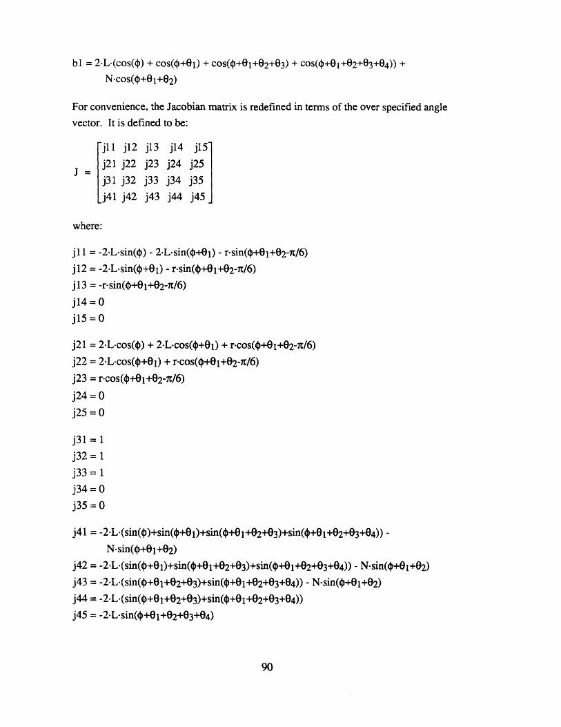
bl = 2-L-(cos(o) + cos(0+01) + cos(4+0 1+e2+03) + cos(4+01+02+03+0 4 )) +N-cos(0+0 1+02)
For convenience, the Jacobian matrix is redefined in terms of the over specified angle
vector. It is defined to be:
jll j12 j13 j14 j15-
j21 j22 j23 j24 j25
j31 j32 j33 j34 j35
j41 j42 j43 j44 j45
where:
jll = -2-L.sin(o) - 2-L-sin(4+01) - r-sin(0+01+02-nx/6)
j 12 = -2-L-sin(i+01) - r-sin(4+01+02-ic/6)
j 13 = -r-sin(O+01+02-n/6)
j14=0
j15 =0
j21 = 2-L*cos(o) + 2-L-cos(4+01) + r-cos(4+01+02-r/6)
j22 = 2-L-cos(0+01) + r-cos(4+01+02-7t/6)
j23 = r-cos(+01÷+02-nr/6)
j24 = 0
j25 = 0
j31 = 1
j32 = 1
j33 = 1j34 = 0j35 = 0
j41 = -2-L.(sin(o)+sin(4+01)+sin( +01+02+03)+sin(Q+01+02+03+04)) -N-sin(4+81+02)
j42 = -2.L.(sin(#+01)+sin(4+01 +02+03)+sin(0+01+02+03+04)) - N.sin(+01 +02)j43 = -2-L-(sin(0+01+02+03)+sin(4+01+02+03+04)) - N-sin(4+01+02)j44 = -2.L.(sin(4+01+02+03)+sin(+01O+012+03+04))
j45 = -2-L-sin(4+01+02+03+04)

It is important to note that the over specified Jacobian matrix, multiplied by the
transformation matrix T, is equivalent to the Jacobian matrix given in Appendix A. That
is:
J(4x5).T = J(4x4)
The potential energy term added by the environmental contact at the end of foot 2 is
given by:
0 0 0 0
j41 j42 j43 j44 j45
Let H-1 be the inverse transformed inertia matrix:
H -' = (TT.M.T)- 1
The state space equations are:
dx = A.x + B-u
y = C.x + D-u
where:
x = [xbody Ybody Obody x21
u = [xbcmd Ybcmd Obcmd x2cmd]
A= [J T H '-TT JT Kd J .T- H-' TT .(JT .-K -8V)I(4x4) 0(4x4)
B= J .T H "' -TT .jT Kd J-T- H-• T JT • Kp0(4x4) 0(4x4)
°00010000000100
0 000001
00000001

S0000000000000000D =00000000000o 00000
As can plainly be seen from these equations, the response of the system will vary as a
function of the configuration dependent effective inertia matrix. The gains chosen after
experimental testing are kp = [1000, 500, 8, 100] and kd = [100, 50, 8, 10].
The analytical response of the LIBRA with these gains is shown in two domains: plots
of the roots of the characteristic equation for the various representative configurations,
and as bode plots for one configuration at Ybody = 0. The eighteen configurations chosen
for testing are:
Xbody = 9 cm, Obody = 0, x2 = 18 cm, ybody = 0.14, 0.12, 0.10, 0.08, 0.06, 0.04, 0.02,
0.00, -0.02, -0.04, -0.06, -0.08, -0.10, -0.12, -0.14, -0.18, and -0.20
The roots for these configurations are shown in Figure C2. However, as the scale is so
large it is difficult to extract meaningful information. A figure of the dominant poles is
given in Figure C3. As can be seen in Figure C3, some of the configurations appear to be
under damped. However, since the significant damping in the motor gearheads is not
included in the analysis, the actual system will respond in a more damped manner.

Poles of LIBRA for Y(body) from -0.20 -> 0.14
Fig. C2: Poles of the LIBRA for Ybody from -0.20m -> 0.14m
3C
20
10
-104
-20(
-30(

+
Ybody = 0.0
Ybody = -0.2\, :
+ -- 10
8
6
4
2
0
nTM
0 Re
Sroay - W.&
Fig. C3: Dominant poles of the LIBRA for Ybody from -0.20m -> 0.14 m
The dominant Bode plots of the system for the chosen configuration of Ybody = 0 are
given in Figures C4 through C6. The design goal is for the system to have a bandwidth
of 6 Hz. For our system, it is desirable for the three free control variables (xbody, Ybody
and Obody) to have close to the same bandwidth, and for the constrained control variable
(xfoot) to have a much lower bandwidth. The only input variable to output variable loops
with magnitudes above -3dB are the loops for the xbody position variables, ybody position
variables and Obody position variables. This is expected, since the xbody, Ybody and 9 body
position variables have the highest control gains by a considerable amount. The xfoot
position loop has very low magnitudes, since it is largely constrained by the environment.
+.. -+ +'••

If excessive coupling were found between one of these input variables and a different
output variable, that control loop would also have high magnitude gains. Since no such
loops are found, the coupling is not excessive in this configuration.
As can be seen in Figure C4, the analysis of the xbody position loop yielded a
bandwidth of 5.2 Hz. This is slightly lower than desired, but still very acceptable. Both
the gain margin and phase margin are large, indicating good stability.
O
-10
-20
.•-n10
11M
0
2-100CL
10
101Frequency (rad/sec)
102
102n n I I n I l i101
101Frequency (rad/sec)
Fig. C4: Bode plot for the xbody position variable
0
Figure C5 shows the Ybody position control loop. The bandwidth of this loop is even
higher than that of the xbody position control loop, being close to 7 Hz. Even though this
is over the desired bandwidth of 6 Hz, it is still acceptable. The additional damping of
the actuators that is not modeled will lower the bandwidth of the actual system. Once
again, the phase margin and gain margins are large, indicating good stability.
100
.. .........., ... ...·........· ..... . ... .... . .... .I............· ... ......· ......·.....·
---- ---------- ~-- ........ ....... .... .... ... .... ..·-··- --· ·-- ·-
2........~~~~............... I .·.\. r. ........ r ............. . .h..-..
0o
...........................
.............. ................... ----------····----- ·--- ···------- ·- ·-- ··-................................................. .......
_-3)

CPpv
a,'p
rr3
Frequency (rad/sec)
200
. 0 . .
-100
10 o 101 10 2Frequency (rad/sec)
Fig. C5: Bode plot for the Ybody position variable
Figure C6 shows the control loop for the Obody position. Its bandwidth is near 5.6 Hz,
which is still acceptable. Like the other two loops, the control loop for Obody shows good
stability.
)2

S-10
-20
-301(
LUU
100
0
i -100
-")n
)2
100 101 102Frequency (rad/sec)
Fig. C6: Bode plot for the Obody position variable
While the dynamic model yields bandwidths that are near the desired in this
configuration, the unmodeled damping in the actuators lowers the bandwidth of the actual
system. The bandwidths are all close to each other as desired, and little coupling between
control variables is seen. Thus the linear analysis of the system using gains chosen
experimentally shows that the system still meets the design goals for the gains.
--
..... ...... ....... ..... ... .... ... ..... ...... ....- -.-.-.-
..... ............ .... .................. .....' .? ... ......... ..... ........ .. ...... ...... .i. ..?... i.. .
I

Appendices References
1C and H sales Co.P.O. Box 5356, 2176 East Colorado Blvd.,Pasadena, CA, 91107
2National Semiconductor2900 Semiconductor Drive, P.O. Box 58090Santa Clara, CA, 95052-8090
3Gerber Electronics128 Carnegie RowNorwood, MA, 02062
4 Newark Electronics248 Pleasant St.Methuen, MA, 01844-7195
5Allied Electronics, Inc., 1-800-433-5700