Embed Size (px)
Citation preview

Misr J. Ag. Eng., July 2009 1299
VALIDATION OF SURFACE IRRIGATION MODEL SIRMOD UNDER CLAY LOAM SOIL CONDITIONS IN
EGYPT Mehana, H. M. **, El-Bagoury, K. F. *, Hussein, M. M. **
and El-Gindy, A.M.* ABSTRACT
Surface irrigation (gravity) is the most dominant method currently accounts for 80-85% of irrigation water use in Egypt and surface application is by far the dominant irrigation method applied throughout the world. However, water use efficiencies with surface irrigation methods tend to be low. In recent years a number of surface irrigation simulation models for assessing surface irrigation system performance have been developed. One of the most commonly used models SIRMOD, developed by Utah State University, has seen wide use and evaluation throughout the world particularly by researchers and has been shown to offer potential for increasing surface irrigation water use efficiencies. The use of the SIRMOD model as a management tool for improving irrigation efficiencies was found to be a valuable aid. This study aims to validate SIRMOD model for using in Egypt under clay loam soil conditions. The SIRMOD model adequately describes advance and recession times and infiltrated depth under experimental site conditions for the furrow irrigation practice. In particular, for the experimental site the SIRMOD model provided acceptable predictions for 75 m and 50 m furrow lengths under 0.2% field slope, and for 100 m, 75 m and 50 m furrow lengths under 0.5% field slope at the 1st irrigation. For that, the good predicted values were for the later irrigations than the first one, due to the good relationship between the predicted and measured infiltration depths obtained from SIRMOD model which has high accuracy degree for furrow irrigation management decisions. Generally, predicted advance, recession times and infiltrated depth were highly correlating with measured one at 0.2% field slope more than 0.5% field slope for the two irrigations. Keywords: SIRMOD model – Furrow irrigation – Soybean – Clay loam sol *Agri. Eng. Dep., Fac. of Agric. Ain Shams Univ., Cairo, Egypt ** Water Relations & Field Irr. Dept. National Research Centre, Cairo, Egypt.
Misr J. Ag. Eng., 26(3): 1299- 1317 IRRIGATION AND DRAINAGE

Misr J. Ag. Eng., July 2009 1300
INTRODUCTION urface irrigation methods within Egypt are currently responsible for greater than 85% of the total irrigated areas and hence make up the dominant method of irrigating both crops and trees. Although
well designed and managed furrow-irrigated systems have the potential to operate at application efficiencies above 90% (Faulkner et al. 1998), many furrow systems operate at significantly lower efficiencies. One of the major constraints to the improvement of furrow irrigation performance has been the difficultly in assessing the many variables associated with furrow irrigation systems and their interactions, and to utilize these in irrigation management. One potential for improving the efficiency and performance of furrow irrigation systems lies in the use of simulation models to simulate and predict furrow irrigation performance and assess changes in management variables, which can lead to improvements in irrigation efficiency. A number of such models have been developed which aim to simulate surface irrigation systems. A few of these models have also been developed into user-friendly computer programs with the ultimate aim of being used by irrigation practitioners as a management tool such as SIRMOD model (Walker, 1998). The SIRMOD model (Walker, 1998) simulates the hydraulics of surface irrigation (border, basin and furrow) at the field level. The simulation routine used in SIRMOD is based on the numerical solution of the Saint-Venant equations for conservation of mass and momentum as described by Walker and Skogerboe (1987). Inputs required for the model to simulate an irrigation event include the infiltration characteristic, hydraulic resistance (Manning’s n), furrow geometry, furrow slope, furrow length, inflow rate and advance cut-off time. Of these required inputs, the most difficult to determine adequately are the infiltration characteristics and the furrow inflows which often require either relatively expensive equipment or significant periods of time and skilled operators. These inputs have also been found to be the most sensitive in the SIRMOD model (McClymont et al. 1996). It should also be noted that a number of assumptions made in the SIRMOD model were not always present in the field investigations. These included a step inflow rate to the furrow, which was rarely found in the field data to due
S

Misr J. Ag. Eng., July 2009 1301
variations in the hydraulic head at the outlets over the irrigation periods. Infiltration characteristics of a furrow are represented in the SIRMOD model with the Kostiakov-Lewis infiltration equation, which is given by:
Z = k ta + f0 t
where Z is cumulative infiltration (m3/m furrow); t is the time (min) that water is available for infiltration; a, k are fitted parameters; and f0 (m3/min/m furrow) is the steady or final infiltration rate (Walker and Skogerboe, 1987). Infiltration characteristics can be determined from the furrow advance rate as described by McClymont and Smith (1996). The remaining input parameters, furrow geometry, furrow slope and furrow length can be easily measured and the Manning’s n coefficient is generally used as a ‘calibrating’ parameter. The output from the model includes the advance and recession characteristics, ultimate distribution of infiltrated water and parameters related to water application, storage, efficiencies and runoff hydrographs. Many surface irrigation systems are designed and/or managed in such a manner that irrigation efficiency is low. Some of the problems associated with furrow irrigation methods are: 1) loss of water by runoff and deep percolation, 2) low uniformity of water application, and 3) high labor and management requirements (Rogers, 1995). The distribution uniformity of an irrigation system depends on both the system characteristics and on managerial decisions (Pereira, 1999). The distribution uniformity of different types of irrigation will be influenced by different factors that are characteristic of the particular system. Surface irrigation is influenced primarily by soil intake characteristics. Distribution uniformity (DU) is usually defined as a ratio of the smallest accumulated depths in the distribution to the average depths of the whole distribution. The largest depths could also be used to express DU, but since the low values in irrigation are more critical, the smallest values are used (Burt et al., 1997). The average of the smallest depths in the field over the portion of the field. This term is used in the numerator of the DU calculation. A commonly used fraction is the lower quarter, which has

Misr J. Ag. Eng., July 2009 1302
been used by the United States Department of Agriculture (USDA, 1997) since the 1940s. This definition has proven useful in irrigated agriculture (ASCE, 1978) and leads to the definition of the average low-quarter depth, dlq. Thus, the average accumulated depth in the quarter of the field receiving the smallest depths is given by (Burt et al., 1997):
Where: davg is the total volume accumulated in all elements [m3] divided by the total area of all the elements [m2]. The area of an element depends on the crop being irrigated. In row crops, such as soybean, the elemental area will be the entire field as there is a crop at every point in the field. These definitions allow the elements to be of different sizes by using area weighting (Burt et al., 1997).
MATERIALS AND METHODS To validate the model, observed data was undertaken at the Experimental Farm of the Faculty of Agriculture, Ain Shams University, Kalubia Governorate to represent the old alluvial soil of the Nile Delta. Furrow (with gated pipes) irrigated soybean was selected along two summer growing seasons 2007 and 2008. The furrows were 15 cm depth and 70 cm spacing and leveled using laser technique.
- Soil and irrigation water analysis: Soil and irrigation water analysis were conducted according to standard procedures and represented in Table (1, 2 and 3). Two slopes were selected 0.2% and 0.5%. The experimental area was divided into two plots (100 m x 11 m) with 2.6 m free between plots. Each plot divided into three subplots (100 m x 2.8 m, 75 m x 2.8 m, and 50 m x 2.8 m) with 1 m spacing between subplots. Soybean was planted in 1st June, and harvested at 5th October, 2007 and 2008 growing seasons. The plants were 20 cm apart in each row, double side cultivation. The inflow to every furrow was 2 l/s. the total volume of irrigated water per season was 3200 m3/season at the two seasons (2007 – 2008), the same amount of irrigation water was applied. The cutoff time differed from
Average low quarter depth (dlq) DUlq =
Average depth of water accumulated in all elements (davg)

Misr J. Ag. Eng., July 2009 1303
treatment to another depending on furrow length. The plants putted in the crest of the furrow, for that the Manning values were 0.04 for the 1st irrigation and 0.03 for the later irrigations. Table (1): Some physical properties of Shalaqan site.
F.C.= field capacity (%); PW.P.=permanent welting point (%), F.C. and PWP were determined as percentage in weight; B.D.= bulk density(g/cm3); WHC= available water holding capacity(mm/m); C.L.= clay loam. Table(2 ) : Some chemical properties of Shalaqan site.
Table (3): Some chemical data of irrigation water at Shalaqan site.
- Model validation: Three different furrow lengths 50, 70 and 100 m and two slopes 0.2 and 0.5 % were selected to validate the SIRMOD. Furrow geometry was measured (as an average of 30 cross sections of furrows, Table (4)) manually by a locally manufactured furrow profile meter Fig. 2. and data. Advance and recession times can be taken manually using markers at known distances (25 m).
Sample depth, cm
Particle Size Distribution, % F.C.
%
W.P.
%
B.D.
g/cm3 Texture
class C.
Sand F.
Sand Silt Clay
0-30 3.2 36 19.1 41.7 28 18 1.30 C.L
30-60 3.1 33.2 20.5 43.2 31 20 1.44 C.L
60-100 4.8 28.9 26.1 40.2 29 16 1.46 C.L
Sample depth,
cm pH
Ec dS/m
Soluble Cations, meq/L Soluble Anions, meq/L
Ca++ Mg++ Na+ K+ CO3-- HCO3
- SO4-- CL-
0-30 8.1 5.7 22.2 9.4 2.4 1.6 - 1 25.7 9.9
30-60 8.2 2.4 9.8 8.5 2.1 3.5 - 1.3 16.4 6.2
60-100 8.4 2.1 8.7 5.2 1.7 2.5 0.8 1.5 11.3 4.5
pH EC dS/m
Soluble Cations, meq/L Soluble Anions, meq/L SAR
Ca++ Mg++ Na+ K+ HCO3- SO4
-- CL--
7.9 0.55 1.63 0.77 4.55 1.2 2.8 0.09 5.26 4.11

Misr J. Ag. Eng., July 2009 1304
Table (4): Unit width flow cross section of furrows. Parameter Measured value, m Top width 0.543 Middle width 0.395 Bottom width 0.121 Maximum depth 0.145
Fig. 1. Locally manufactured furrow profile meter
30cm
80 cm

Misr J. Ag. Eng., July 2009 1305
- SIRMOD model screens: 1- Data input: Data input to the SIRMOD software involves two activities: (1) defining the characteristics of the surface irrigation system under study; and (2) defining the model operational control parameters. A data entry screen is inserted on the main screen with three user-selectable tabs: (1) Field Geometry & Topography; (2) Infiltration Functions; and (3) Flow Cross-Section. Fig. 2. shows the field characteristic data entry form opened to the Field Geometry/Topography page. The geometry and topography of the surface irrigated field is described by the following parameters: Manning roughness, n, for the first irrigations; Manning roughness, n, for later irrigations; Field length; Field width; Unit spacing for borders and basins, or furrow spacing; Field cross-slope; Three slope values in the direction of flow; and Two distance parameters associated with the three slopes. The SIRMOD software is capable of simulating fields with a compound slope as shown in Fig. 2. Three slopes are located in the field by two distance values as shown. When the field has only one slope, the same value needs to be entered for all three slopes and both distance values should be set to the field length.
2-Type of Simulation Model The SIRMOD software includes three modeling choices: (1) kinematic-wave model; (2) zero-inertia model; and (3) hydrodynamic model. The default is the hydrodynamic model. The user may choose a particular model for simulation by clicking their associated check boxes (Fig. 3.).
Fig. 2. Field Characteristics Input Screen

Misr J. Ag. Eng., July 2009 1306
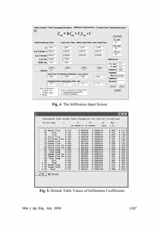
3- Infiltration Functions The tabbed notebook where infiltration functions are defined is shown in Fig. 4. This is the most critical component of the SIRMOD software. Four individual infiltration functions are required: (1) a function for first conditions under continuous flow; (2) a function for later irrigations under continuous flow; (3) a function for first irrigations under surge flow; and (4) a function for later irrigations under surge flow. Each infiltration function requires four parameters, k, a, fo, and C. Immediately below the four infiltration coefficients for the various surface irrigation regimes are four buttons labeled “Table Values”. These buttons access four default infiltration data sets as illustrated in Fig. 5. These can be selected by clicking on their radio buttons.
Fig. 3. Inflow controls input
Misr J. Ag. Eng., July 2009 1307
Fig. 4. The Infiltration Input Screen
Fig. 5. Default Table Values of Infiltration Coefficients

Misr J. Ag. Eng., July 2009 1308
4- Simulation: Once the input and control data have been entered, the simulation can be executed by clicking on the button. The simulation screen will appear and the run-time plot of the advance and recession profiles will be shown as illustrated in Fig. 6. There are three important regions in the simulation screen. The first occupies the upper one-half of the screen and plots the surface and subsurface movements of water as the advance and recession trajectories are computed. The target or required depth of application is plotted as Zreq
so that when an infiltrated depth exceeds this value the user can see the loss of irrigation water to deep percolation (The subsurface profile color changes as the depth exceeds Zreq). In the lower right side of the screen a summary of the simulated irrigation event will be published after the completion of recession. The bottom four edit windows give a mass balance of the simulation, including an error term describing the computed differences between inflow, infiltration, and runoff. As a rule an error less than 5% is acceptable – most simulations will have errors of about 1%. In the lower left side of the screen, a runoff hydrograph will be plotted.
Fig. 6. Simulation Screen

Misr J. Ag. Eng., July 2009 1309
5- Plotted Output Clicking on the Plotted Results option under the Results menu reveals the plotting screen shown in Fig. 7. Three sets of data (Advance, Runoff, and End depth) can be plotted by checking the appropriate box in the output screen shown above.
RESULTS OF MODEL VALIDATION AND DISCUSSION
The advance, recession times and infiltrated depth of the selected treatment (4 furrow each) were measured. The infiltrated depth was measured by determining the opportunity time (Advance time – recession time).
The input data to the model program are, furrow length, and slope, Manning values were 0.04 for the 1st irrigation and 0.03 for the later irrigation, as well as the furrow geometry and the cutoff time, to simulate the hydraulics of surface irrigation under the actual experiment treatments. Figs. 8, 9, 10, 11, 12 and 13 show the relationship between the measured advance, recession times, and infiltrated depth, and those predicted by the SIRMOD model.
Fig. 7. Graphical Output Screen
Misr J. Ag. Eng., July 2009 1310
0
10
20
30
40
50
0 50 100
Measured advance time, min
Pred
icte
d ad
vanc
e tim
e, m
inFirst irrigation Third irrigation
R2 = 0.92 Y= 0.98965 + 0.15828 X
R2 = 0.93 Y= 1.379 + 0.1119 X
50
100
150
200
250
50 100 150 200 250Measured recession time, min
Pred
icte
d re
cess
ion
time,
min
First irrigation Third irrigation
R2 = 0.95 Y= 73.364 + 0.318X
R2 = 0.94 Y= 66.129 + 0.3147 X
0.04
0.045
0.05
0.055
0.06
0.065
0.04 0.09 0.14 0.19 0.24 0.29
Measured infiltrated depth, m
Pred
icte
d in
filtr
ated
dep
th, m First irrigation Third irrigation
R2 = 0.93 Y= -0.4866 + 7.771 X – 36.91 X2 + 57.522 X3
Y= -0.7233 + 15.487 X – 100.355 X2 + 212.045 X3 R2 = 0.71
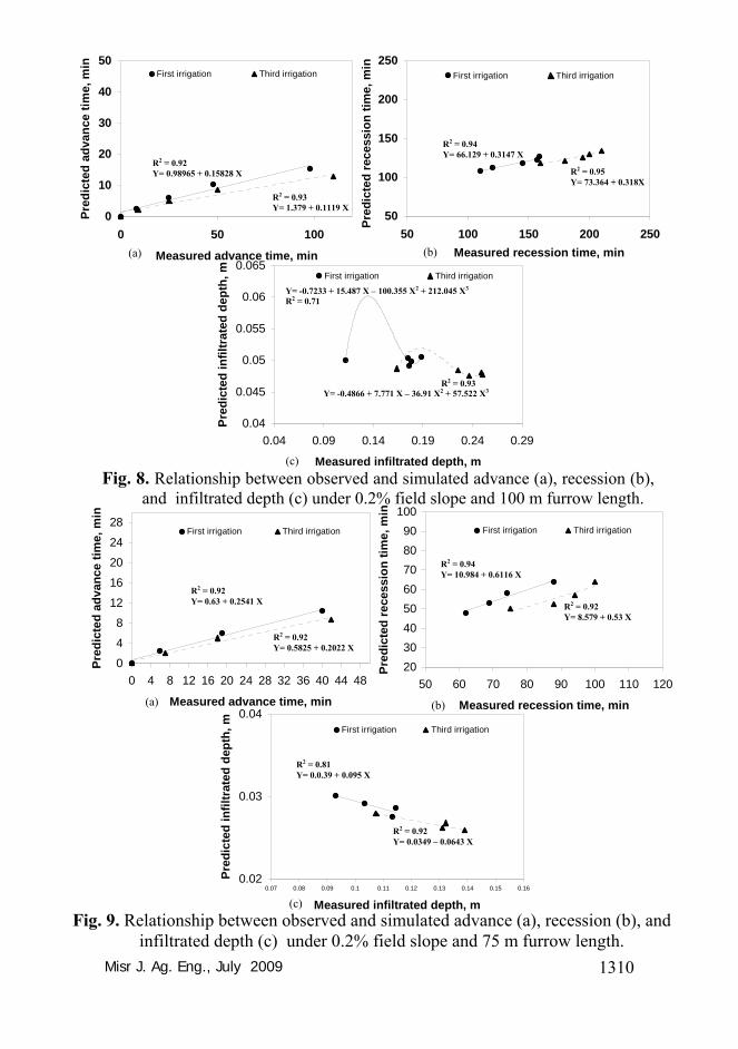
Fig. 8. Relationship between observed and simulated advance (a), recession (b), and infiltrated depth (c) under 0.2% field slope and 100 m furrow length.
0.02
0.03
0.04
0.07 0.08 0.09 0.1 0.11 0.12 0.13 0.14 0.15 0.16
Measured infiltrated depth, m
Pred
icte
d in
filtr
ated
dep
th, m First irrigation Third irrigation
Fig. 9. Relationship between observed and simulated advance (a), recession (b), and infiltrated depth (c) under 0.2% field slope and 75 m furrow length.
0
4
8
12
16
20
24
28
0 4 8 12 16 20 24 28 32 36 40 44 48
Measured advance time, min
Pred
icte
d ad
vanc
e tim
e, m
in
First irrigation Third irrigation
R2 = 0.92 Y= 0.63 + 0.2541 X
R2 = 0.92 Y= 0.5825 + 0.2022 X
2030405060708090
100
50 60 70 80 90 100 110 120
Measured recession time, min
Pred
icte
d re
cess
ion
time,
min
First irrigation Third irrigation
R2 = 0.94 Y= 10.984 + 0.6116 X
R2 = 0.92 Y= 8.579 + 0.53 X
R2 = 0.92 Y= 0.0349 – 0.0643 X
R2 = 0.81 Y= 0.0.39 + 0.095 X
(a) (b)
(c)
(a) (b)
(c)
Misr J. Ag. Eng., July 2009 1311
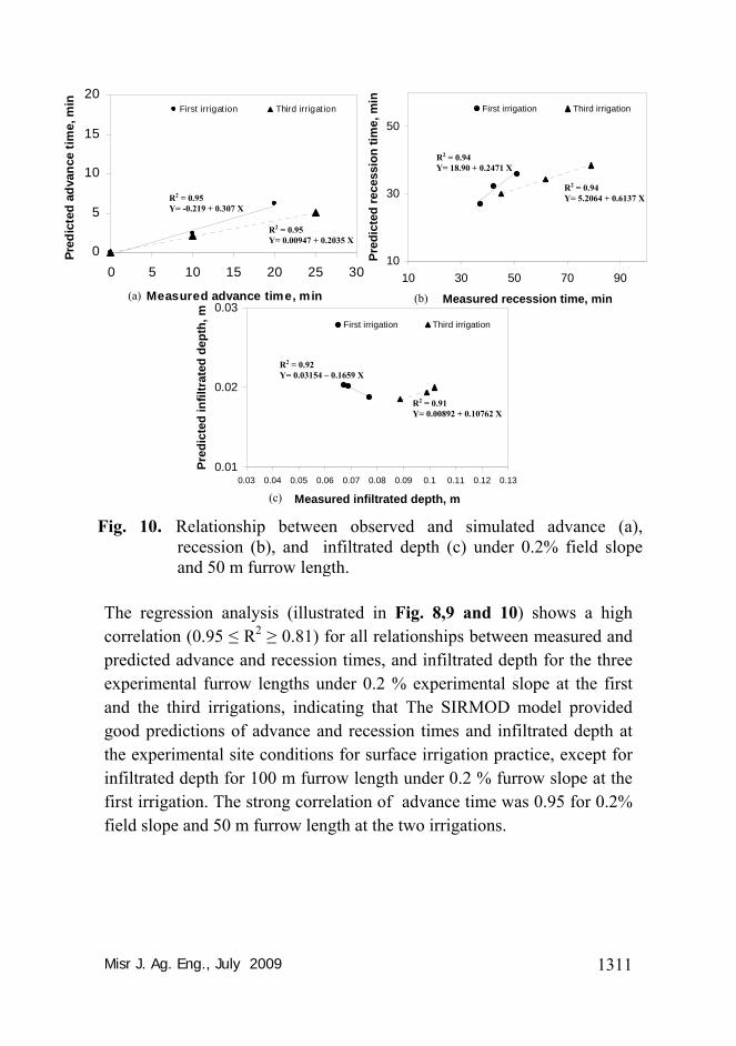
The regression analysis (illustrated in Fig. 8,9 and 10) shows a high correlation (0.95 ≤ R2 ≥ 0.81) for all relationships between measured and predicted advance and recession times, and infiltrated depth for the three experimental furrow lengths under 0.2 % experimental slope at the first and the third irrigations, indicating that The SIRMOD model provided good predictions of advance and recession times and infiltrated depth at the experimental site conditions for surface irrigation practice, except for infiltrated depth for 100 m furrow length under 0.2 % furrow slope at the first irrigation. The strong correlation of advance time was 0.95 for 0.2% field slope and 50 m furrow length at the two irrigations.
Fig. 10. Relationship between observed and simulated advance (a), recession (b), and infiltrated depth (c) under 0.2% field slope and 50 m furrow length.
0
5
10
15
20
0 5 10 15 20 25 30
Measured advance time, min
Pred
icte
d ad
vanc
e tim
e, m
in First irrigat ion Third irrigat ion
R2 = 0.95 Y= -0.219 + 0.307 X
R2 = 0.95 Y= 0.00947 + 0.2035 X
10
30
50
10 30 50 70 90
Measured recession time, min
Pred
icte
d re
cess
ion
time,
min
First irrigation Third irrigation
R2 = 0.94 Y= 5.2064 + 0.6137 X
R2 = 0.94 Y= 18.90 + 0.2471 X
0.01
0.02
0.03
0.03 0.04 0.05 0.06 0.07 0.08 0.09 0.1 0.11 0.12 0.13
Measured infiltrated depth, m
Pred
icte
d in
filtr
ated
dep
th, m First irrigation Third irrigation
R2 = 0.91 Y= 0.00892 + 0.10762 X
R2 = 0.92 Y= 0.03154 – 0.1659 X
(a) (b)
(c)
Misr J. Ag. Eng., July 2009 1312
0
10
20
30
0 10 20 30 40 50 60 70 80 90 100 110
Measured advance time, min
Pred
icte
d ad
vanc
e tim
e, m
in
First irrigation Third irrigation
R2 = 0.90 Y= 1.0768 + 0.12428 X
R2 = 0.89 Y= 1.2239 + 0.0957 X
50
100
150
200
250
50 100 150 200 250
Measured recession time, min
Pred
icte
d re
cess
ion
time,
min
First irrigation Third irrigation
R2 = 0.91 Y= 81.045 + 0.1963 X
R2 = 0.90 Y= 220.729 – 1.3589 X + 0.00394 X2
0.04
0.042
0.044
0.046
0.048
0.05
0.052
0.04 0.06 0.08 0.1 0.12 0.14 0.16 0.18 0.2 0.22 0.24 0.26 0.28 0.3
Measured infiltrated depth, m
Pred
icte
d in
filtr
ated
dep
th, m First irrigation
Third irrigation
R2 = 0.92 Y= 0.6376 – 7.5053 X + 31.4715 X2 – 43.812 X3
R2 = 0.92 Y= 0.3587 – 5.985 X + 27.835 X2 – 50.521 X3
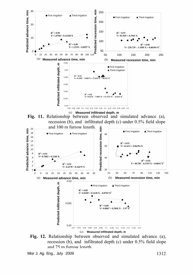
Fig. 11. Relationship between observed and simulated advance (a), recession (b), and infiltrated depth (c) under 0.5% field slope and 100 m furrow length.
20
40
60
80
10 30 50 70 90 110 130 150
Measured recession time, min
Pred
icte
d re
cess
ion
time,
min
First irrigation Third irrigation
0
2
4
6
8
10
12
14
16
18
20
0 5 10 15 20 25 30 35 40 45 50
Measured advance time, min
Pred
icte
d ad
vanc
e tim
e, m
in
First irrigation Third irrigation
R2 = 0.91 Y= 0.7083 + 0.2185 X
R2 = 0.91 Y= 0.6378 + 0.16675 X
0.02
0.025
0.03
0.07 0.075 0.08 0.085 0.09 0.095 0.1 0.105 0.11 0.115 0.12 0.125 0.13
Measured infiltrated depth, m
Pred
icte
d in
filtr
ated
dep
th, m First irrigation Third irrigation
R2 = 0.89 Y= 0.0067 + 0.3856 X – 1.97 X2
R2 = 0.89 Y= 0.0185 + 0.1638 X – 0.8769 X2
Fig. 12. Relationship between observed and simulated advance (a), recession (b), and infiltrated depth (c) under 0.5% field slope and 75 m furrow length.
R2 = 0.92 Y= 48.785 – 0.3353 X + 0.0043 X2
R2 = 0.93 Y= 43.633 + 0.06394 X
(a) (b)
(c)
(a) (b)
(c)

Misr J. Ag. Eng., July 2009 1313
The regression analysis (illustrated in Fig. 11, 12 and 13 ) shows a high correlation (R2 ≥ 0.89) for all relationships between measured and predicted advance and recession times, and infiltrated depth for the three experimental furrow lengths under the two experimental slopes at the first and the third irrigations, indicating that The SIRMOD model provided good predictions of advance and recession times, and infiltrated depth at the experimental site conditions for surface irrigation practice. The relationship between the measured and predicted recession time has the same trend, but the highly correlating was for 75 m furrow length under the 0.5% field slope at the two irrigations, and the lower value of correlation was 0.89 for 50 m furrow length under 0.5% field slope but it acceptable for users to simulate or predict the recession time.
Fig. 13. Relationship between observed and simulated advance(a), recession (b), and infiltrated depth (c) under 0.5% field slope
0
1
2
3
4
5
6
7
8
9
10
0 2 4 6 8 10 12 14 16 18 20 22 24 26 28 30 32 34 36
Measured advance time, min
Pred
icte
d ad
vanc
e tim
e, m
in
First irrigation Third irrigation
R2 = 0.91 Y= 0.5691 + 0.15 X
R2 = 0.91 Y= 0.525 + 0.131 X
20
30
40
50
60
10 30 50 70 90 110
Measured recession time, min
Pred
icte
d re
cess
ion
time,
min
First irrigation Third irrigation
R2 = 0.89 Y= 31.138 + 0.109 X
R2 = 0.92 Y= 30.85 + 0.05763 X
0.01
0.02
0.03
0.04
0.05
0.065 0.075 0.085 0.095 0.105 0.115 0.125 0.135
Measured infiltrated depth, m
Pred
icte
d in
filtr
ated
dep
th, m First irrigation Third irrigation
R2 = 0.92 Y= 0.0208 - 0.00598 X
R2 = 0.92 Y= 0.00427 + 0.4179 X – 2.119 X2
(a) (b)
(c)
Misr J. Ag. Eng., July 2009 1314
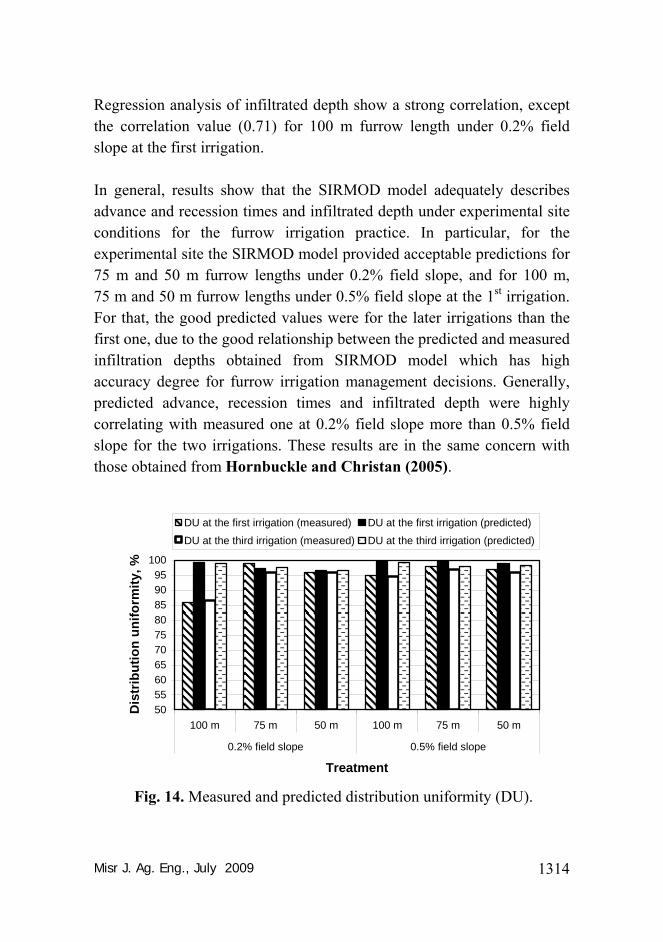
Regression analysis of infiltrated depth show a strong correlation, except the correlation value (0.71) for 100 m furrow length under 0.2% field slope at the first irrigation.
In general, results show that the SIRMOD model adequately describes advance and recession times and infiltrated depth under experimental site conditions for the furrow irrigation practice. In particular, for the experimental site the SIRMOD model provided acceptable predictions for 75 m and 50 m furrow lengths under 0.2% field slope, and for 100 m, 75 m and 50 m furrow lengths under 0.5% field slope at the 1st irrigation. For that, the good predicted values were for the later irrigations than the first one, due to the good relationship between the predicted and measured infiltration depths obtained from SIRMOD model which has high accuracy degree for furrow irrigation management decisions. Generally, predicted advance, recession times and infiltrated depth were highly correlating with measured one at 0.2% field slope more than 0.5% field slope for the two irrigations. These results are in the same concern with those obtained from Hornbuckle and Christan (2005).
50556065707580859095
100
100 m 75 m 50 m 100 m 75 m 50 m
0.2% field slope 0.5% field slope
Treatment
Dis
trib
utio
n un
iform
ity, %
DU at the first irrigation (measured) DU at the first irrigation (predicted)
DU at the third irrigation (measured) DU at the third irrigation (predicted)
Fig. 14. Measured and predicted distribution uniformity (DU).

Misr J. Ag. Eng., July 2009 1315
Fig. 14. shows a comparison between the actual distribution uniformity (DU) under the experimental treatments and the predicted by the SIRMOD model. It can be seen that the lowest differences between the predicted and the measured distribution uniformities were by irrigating soybean plants under the shortest experimental furrow lengths ( 50 m and 75 m). Data obtained in Table (5) indicated that the highest soybean yield (2.29, 1.76) ton/fed. were gained by irrigating plants under 75 m furrow length at 0.2% and 0.5% field slopes. The same trend of water use efficiency (WUE) was indicated, whereas the maximum value (0.71) was mentioned by 75 m furrow length and 0.2% field slope. From Fig. 14. and Table (5), it can be concluded that there is a relationship between distribution uniformity, and soybean yield. For that, simulation or prediction of hydraulic characteristics of surface irrigation will be better practical decisions for irrigation management (which furrow length and field slope can be used ? ).
Table 5. The effect of the field slope and furrow length on soybean yield (ton/fed.) and WUE (kg/m3).
Field slope, % Furrow length,
m Seed yield
ton/fed Water use
efficiency, kg/m3
0.2 50 1.18 0.37 75 2.29 0.71 100 1.58 0.49
0.5 50 1.26 0.39 75 1.79 0.56 100 1.87 0.56
CONCLUSION The SIRMOD model adequately describes advance and recession times and infiltrated depth under experimental site conditions for the furrow irrigation practice. In particular, for the experimental site the SIRMOD model provided acceptable predictions for 75 m and 50 m furrow lengths under 0.2% field slope, and for 100 m, 75 m and 50 m furrow lengths under 0.5% field slope at the 1st irrigation. For that, the good predicted

Misr J. Ag. Eng., July 2009 1316
values were for the later irrigations than the first one, due to the good relationship between the predicted and measured infiltration depths obtained from SIRMOD model which has high accuracy degree for furrow irrigation management decisions. Generally, predicted advance, recession times and infiltrated depth were highly correlating with measured one at 0.2% field slope more than 0.5% field slope for the two irrigations.
REFERENCES ASCE (1978). Describing irrigation efficiency and uniformity. J. Irrig.
Drain. Div. 104 (1) 35-41. Burt C.M.; A.J. Clemmens; T.S. Strelkof; K.H. Solomon; R.D.
Bliesner; L.A. Hardy; T.A. Howell and D.E. Eisnerhauer (1997). Irrigation performance measures: Efficiency and uniformity. J. Irrig. Drain. Eng. 123 (6) 423-442
Rogers D. H. (1995). Managing furrow irrigation systems. IRRIGATION MANAGEMENT S E R I E S, University of Nebraska-Lincoln.
Faulkner R.D; J. Douglas and D. MacLeod (1998). The Hydrology of Surface Irrigation for Cotton. Proceedings of National IAA Conference “Water is Gold”. Brisbane, May 1998, pp373-381. ISBN 0 7242 7281 X.
Hornbuckle, J. W. and E. W. Christen (2005). Use of SIRMOD as a Quasi Real Time Surface Irrigation Decision Support System. MODSIM 2005 International Congress on Modelling and Simulation. Melbourne, Australia, Modelling and Simulation Society of Australia and New Zealand.
McClymont, D.; S. Raine and R. Smith (1996). The Prediction of Furrow Irrigation Performance using the Surface Irrigation Model SIRMOD. 13th National Conference. Irrigation Association of Australia. Adelaide.
McClymont, D. and R. Smith (1996). Infiltration Parameters from Optimization on Furrow Irrigation Advance Data. Irrigation Science. 17:15-22.
Pereira L.S. (1999). Higher performance through combined improvements in irrigation methods and scheduling: a discussion. Agric. Water Manage. 40 (2) 153-169.

Misr J. Ag. Eng., July 2009 1317
Walker, W. (1998). SIRMOD – Surface Irrigation Modeling Software. Utah State University.
Walker, W. and G. Skogerboe (1987). Surface Irrigation Theory and Practice. Prentice-Hall, New York.
USDA. (1997). SRFR v3. US Department of Agriculture. US Water Conservation Laboratory, Phoenix. AZ.
الملخص العربي
تحت SIRMODالتحقق من صالحية استخدام برنامج محاكاة الري السطحي طميية في مصر - ظروف التربة الطينية
٤، عبد الغني محمد الجندي٣، محمد مرسي حسين٢، خالد طاھر الباجوري١ھاني محمد مھنا
راھن، حوالي ر% ٨٥ – ٨٠يستھلك نظام الري السطحي، في الوقت ال اه ال ي المستخدمة من ميالم ارا كممارسة ري في الع ر انتش اءات استخدام . في مصر، حيث أن ھذا النظام ھو األكث د كف تع
اة رامج المحاك د من ب م نمذجة العدي رة ت مياه الري لھذا النظام منخفضة لذلك وفي السنوات األخيل يم أداءه تحت ظروف الحق ري السطحي لتقي اة المسمي . لل د نموذج المحاك من SIRMODيع
ة دة االمريكي ات المتح ا بالوالي ة يوت ه جامع عته ونفذت ذي وض تخداما وال رامج اس ذه الب ر ھ . أكثدة ائج جي يستخدم ھذا النموذج علي نطاق واسع عالميا وخاصة من جانب الباحثين، حيث أعطي نت
لتحسين يعد استخدام النموذج أداه . لمحاكاة الري السطحي تحاكي تلك المتحصل عليھا في الطبيعة . كفاءة الري السطحى وقد قدم مساعدة ملموسة في ذلك
. طميية في مصر -تھدف ھذه الدراسة للتحقق من مالئمة ھذا النموذج تحت ظروف التربة الطينيةدم الري بالخطوط بشكل عام بينت النتائج أن النموذج أداة جيدة لمحاكاة ي التق والتنبؤ بكال من زمن
ري واالنحسار وكذلك عمق ميا اه تحت ظروف ال ع المي ة توزي را انتظامي ة وأخي ه المترشح بالتربة ة الطيني الخطوط للترب ا مصر –ب ي دلت ة ف دم واالنحسار . طميي ي التق أ لزمن امج تنب يعطي البرن
ة اء عملي ل أثن وكذلك عمق المياه المترشح ذو عالقة ارتباط قوية مع تلك البيانات المقاسة في الحقل . محصول فول الصويا الري خالل موسم نمو حيث يعطي البرنامج تنبأ مقبول تحت ظروف حق
ل خطوط، و% ٠.٢تحت متر ٥٠متر أو ٧٥ذو طول ر و ١٠٠خطوط ألطوالمي ٥٠و ٧٥متامج %. ٠.٥ميل خطوط مقداره تحت متر ا من خالل البرن أ بھ ات المتنب بصفة عامة، كانت البيان
ميل خطوط عنه تحت ظروف % ٠.٢قل تحت ظروف ذات عالقة ارتباط قوية مع المقاسة في الحا والم. ميل خطوط% ٠.٥ أ بھ ات المتنب اتكذلك كان االرتباط بين البيان وي للري ي قاسة ق ي تل الت
.الرية األولي باحث مساعد، قسم العالقات المائية والري الحقلي، المركز القومي للبحوث، مصر ١ جامعة عين شمس، مصر ،ةمدرس بقسم الھندسة الزراعية، كلية الزراع ٢ أستاذ متفرغ، قسم العالقات المائية والري الحقلي، المركز القومي للبحوث، مصر ٣ أستاذ متفرغ، قسم الھندسة الزراعية، كلية الزراعة، جامعة عين شمس، مصر ٤